Roughness on liquid-infused surfaces induced by capillary waves

Abstract

Liquid-infused surfaces (LIS) are a promising technique for reducing friction, fouling and icing in both laminar and turbulent flows. Previous work has demonstrated that these surfaces are susceptible to shear-driven drainage. Here, we report a different failure mode using direct numerical simulations of a turbulent channel flow with liquid-infused longitudinal grooves. When the liquid-liquid surface tension is small and/or grooves are wide, we observe travelling-wave perturbations on the interface with amplitudes larger than the viscous sublayer of the turbulent flow. These capillary waves induce a roughness effect that increases drag. The generation mechanism of these waves is explained using the theory developed by Miles for gravity waves. Energy is transferred from the turbulent flow to the LIS provided that there is a negative curvature of the mean flow at the critical layer. Given the groove width, the Weber number and an estimate of the friction Reynolds number, we provide relations to determine whether a LIS behaves as a smooth or rough surface in a turbulent flow.

1 Introduction

A protective and functional surface coating can be created by lubricating a textured surface with an appropriate liquid. The drag-reducing properties of these liquid-infused surfaces (LIS) have been explored recently both numerically (Fu et al., 2017; Cartagena et al., 2018; Arenas et al., 2019) and experimentally (Van Buren & Smits, 2017; Fu et al., 2019). LIS can also prevent fouling (Epstein et al., 2012), corrosion (Wang et al., 2015) and ice formation (Kim et al., 2012).

The drag-reducing capabilities of LIS for liquid flows is often compared to those of superhydrophobic surfaces (SHS), where air is used as the infused medium. The low viscosity of air is beneficial for drag reduction, but the use of SHS in turbulent applications is restricted by mass diffusion (Ling et al., 2017) and instability of the gas pockets (Seo et al., 2018). For LIS, the mass diffusion is negligible if the liquids are immiscible, and LIS are not susceptible to failure due to hydrostatic pressure (Wong et al., 2011). However, also for LIS, the stability of the interface depends on the texture’s geometry, the surface tension between the two liquids and the contact angle at the liquid-liquid-solid interface. In particular, these surfaces may experience shear-driven drainage of the infused liquid, but this can be mitigated, for example with chemical patterning (Wexler et al., 2015; Fu et al., 2019).

In this paper, we show that capillary motion of the liquid-liquid interface may drastically lower the drag-reducing performance of LIS. In the present study, the surface texture is fixed to longitudinal (streamwise-aligned) grooves. We use direct numerical simulations of a LIS in a liquid turbulent channel flow for frictional Reynolds numbers around $\mathrm{Re}_{\tau}\approx 180$. The employed volume-of-fluid (VOF) framework allows for large interface deformations (low surface tension) and moving contact lines. When the liquid-liquid surface tension is small and/or grooves are wide, we find travelling-wave perturbations on the interface with amplitudes larger than the viscous sublayer of the turbulent flow ($a^{+}\approx 5-8$). These capillary waves induce a roughness effect and increase friction drag.

The detrimental capillary waves develop for viscosity and density ratios of one, which excludes interface instability mechanisms driven by density and viscosity stratification (Boomkamp & Miesen, 1996). Instead, we find that the linear instability can be described by the theory developed by Miles (1957) in the context of two-dimensional gravity waves. This inviscid instability is due to an energy transfer from the external flow to the waves that makes them grow in time at an exponential rate. The energy transfer can occur if (i) there is a negative curvature of the mean velocity profile where it equals the phase speed of a wave, i.e. at the critical layer and, (ii) the critical layer is not too far away from the surface, so that velocity fluctuations due to the wave (dispersive stresses) are non-zero.

The existence of energy transfer is not sufficient for failure of LIS, however. The interface fluctuations also need to grow sufficiently fast to reach large amplitudes that induce roughness effects. Figure 1, which summarises our main contribution, shows three domains, namely rough, smooth and transitional (grey) in a plane spanned by a groove width ($w^{+}$) and a Weber number ($\mathrm{We}^{+}$), both normalised with the viscous length scale. This design map is obtained from the critical-layer theory and provides a means to design LIS that can be predicted to achieve a balance between performance (large $w^{+}$) and stability (smooth domain).

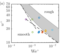
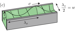
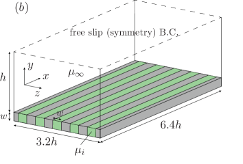
Figure 1: ($a$) Design map for LIS, spanned by $\mathrm{We}^{+}$ and $w^{+}$. Smooth and rough regions are separated using eqs. (12), (14) and (15). Values from simulations with $w^{+0}=18$ are included, with symbols referring to $\mu_{i}/\mu_{\infty}=1$ (), $\mu_{i}/\mu_{\infty}=0.5$ () and $\mu_{i}/\mu_{\infty}=2$ () and colours to $\mathrm{We}=50$ (green), $\mathrm{We}=100$ (blue), $\mathrm{We}=150$ (red), $\mathrm{We}=200$ (yellow) and $\mathrm{We}=400$ (turquoise). Also shown are values with wider grooves, $w^{+0}=36$, with $\mathrm{We}=25$ (purple circle), $\mathrm{We}=50$ (green circle) and $\mathrm{We}=100$ (blue circle). The asymptotic relations (16) and (17) are shown with () and (), respectively. Sketch of ($b$) the channel configuration and ($c$) of a wave on a groove. The infused liquid is shown in green and the solids in grey.

2 Numerical methods and configuration

We consider a fully developed turbulent open channel flow. The flow domain, shown schematically in fig. 1, has the size $(L_{x},L_{y},L_{z})=(6.4h,h+k,3.2h)$, where $x,y$ and $z$ correspond to the streamwise, wall-normal and spanwise directions, respectively, and $h$ is the half-channel height. At the top boundary we impose a free-slip (symmetry) boundary condition (BC). Periodic boundary conditions are imposed in the streamwise and spanwise directions. The streamwise-aligned grooves at the bottom wall have a height $k$, a width $w$ and square cross-section, $k=w$. The fluid-solid ratio is set to $0.5$. The infused and external fluids have the same density $\rho_{i}=\rho_{\infty}=\rho$, but different viscosities ($\mu_{i}$ and $\mu_{\infty}$). We have used grooves of width $w^{+0}=18$. Throughout this paper, $+0$ refers to normalisation using the friction velocity of a regular smooth wall (nominal wall units). A single superscript $+$ refers to normalisation using the friction velocity of each individual case. The corresponding viscous length scale is $\delta_{\nu}=\mu_{\infty}/(\rho u_{\tau})$, where $u_{\tau}$ is the friction velocity.

We impose a constant mass flow rate through a uniform pressure gradient over $0<y<h$, where $y=0$ corresponds to the crest of the texture so that $\mathrm{Re}_{b}=\rho hU_{b}/\mu_{\infty}=2820$, giving $\mathrm{Re}_{\tau}=\rho hu_{\tau}/\mu_{\infty}\approx 180$ (with the pressure gradient implemented as a volume force). Here, $\mathrm{Re}_{b}$ and $\mathrm{Re}_{\tau}$ are Reynolds numbers based on bulk velocity $U_{b}$ and friction velocity $u_{\tau}$, respectively.

Our simulations allow for a moving liquid-liquid-solid contact line with a dynamic contact angle different from the static value, which is $\theta=45\degree$ with respect to the infused liquid. Our method also allows for interface deformation, which is typically quantified by the Weber number, defined as $\mathrm{We}=\rho U_{\mathrm{b}}^{2}h/\gamma$, where $\gamma$ is the surface tension. We have simulated LIS for $\mathrm{We}=100$, $150$ and $200$ and viscosity ratios $\mu_{i}/\mu_{\infty}=0.5$, $1$ and $2$. The Weber number in wall units is $\mathrm{We}^{+}=\rho u_{\tau}^{2}\delta_{\nu}/\gamma=\mu_{\infty}u_{\tau}/\gamma$. It can be noted that the Weber number based on the friction velocity and the width of the grooves is $\mathrm{We}^{+}w^{+}$.

The numerical configuration described above corresponds to an infused liquid consisting of some alkane (with dynamic viscosities similar to that of water (Van Buren & Smits, 2017)), a water channel with $h=0.5$ cm and $U_{\mathrm{b}}=1$ m/s. This results in $\mathrm{Re}_{b}=5000$, which is close to the value in our simulations. A typical surface tension $\gamma=50$ mN/m then results in $\mathrm{We}=100$.

The code used for the simulations is based on the PArallel, Robust, Interface Simulator (PARIS), which employs a VOF method for the multiphase description (Aniszewski et al., 2021; Arrufat et al., 2021). The cited papers also include additional test cases and validations. Height functions are used for curvature calculation for the surface tension. The interface is advected in the manner suggested by Weymouth & Yue (2010) at each substep. This advection scheme conserves the volume of both liquids to a high accuracy. At solid surfaces, a contact angle is imposed by using the height functions and a dynamic contact angle model for VOF based on hydrodynamic theory (Legendre & Maglio, 2015). Details are given in sec. S1 of the supplementary material (SM). Finally, the grid size is $(N_{x},N_{y},N_{z})=(256,640,1024)$, with constant grid spacing in each direction. The flow was converged after $600h/U_{b}$, and statistics were collected over a time of $500h/U_{b}$.

3 Results

3.1 Dependence of drag on Weber number

Figure 2(a) shows an instantaneous snapshot of the liquid-liquid interface, viewed from the top, for $\mathrm{We}=100$ and $\mu_{i}=\mu_{\infty}$. There are oscillations on the interface, due to the finite surface tension, but they remain small. The deformation of the interface increases with $\mathrm{We}$, however. For $\mathrm{We}=200$, significantly larger waves develop on the interface, as shown in fig. 2(b).

The consequences of the waves on the overlying flow can be quantified by the drag reduction

$$\mathrm{DR}=\frac{c_{f}^{0}-c_{f}}{c_{f}^{0}},$$ (1)

where $c_{f}=2\tau_{w}/(\rho U_{b}^{2})$ is the friction coefficient and $\tau_{w}$ is the total stress at the crest plane of the surface (computed from the pressure gradient). Here, $c_{f}^{0}$ is the coefficient of a regular smooth wall at $y=0$. For $\mathrm{We}=100$ and $\mathrm{We}=200$, we obtained $\mathrm{DR}=0.09$ and $\mathrm{DR}=-0.04$, respectively. In other words, the capillary waves observed at $\mathrm{We}=200$ increase frictional drag compared to a smooth and homogeneous surface and have therefore induced failure of the LIS.

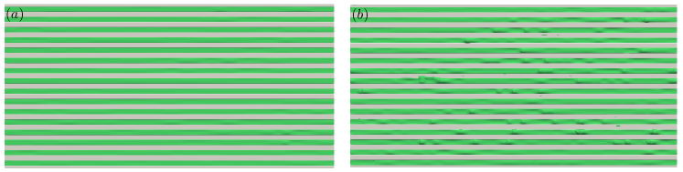
Figure 2: Top view of interfaces (green) and surface (grey) at one instant for $\mu_{i}/\mu_{\infty}=1$ and ($a$) $\mathrm{We}=100$ and ($b$) $\mathrm{We}=200$. The flow is from left to right. The complete domain is shown.

Figure 3 shows $\mathrm{DR}$ for $\mathrm{We}=\{100,150,200\}$ and viscosity ratios $\mu_{i}/\mu_{\infty}=\{0.5,1,2\}$ as a function of the apparent slip length, $b^{+0}$. The slip length $b$ is the distance at which the mean velocity would be zero if linearly extrapolated at the crests of the surface. It is largely unaffected by changes in $\mathrm{We}$, but it increases with decreasing viscosity ratio. In fact, the slip lengths extracted from our numerical simulations with $w^{+}\approx 18$ are well approximated by the slip lengths obtained by solving the Stokes equations for a periodic array of grooves exposed to unit shear (Schönecker et al., 2014) (black line in fig. 3). A similar agreement was observed for smaller grooves ($w^{+}\approx 9$) in turbulent flows by Fu et al. (2017); Arenas et al. (2019).

When the interface is perfectly flat ($\mathrm{We}=0$), the drag reduction can be related to slip length as

$$\mathrm{DR}\approx\frac{b^{+0}}{b^{+0}+U_{b}^{+0}},$$ (2)

where $U_{b}^{+0}$ is the bulk velocity in nominal wall units. This relation – shown in 3 (black line) – can be obtained by neglecting changes in the Reynolds shear stress above a smooth wall (Rastegari & Akhavan, 2015). We observe from fig. 3 that, for $\mathrm{We}=100$ (blue) and $\mathrm{We}=150$ (red), there is a drag reduction ($\mathrm{DR}>0$) for all three viscosity ratios. Moreover, the deviations from (2) are small, confirming that the drag reduction mechanism is indeed slippage. These small deviations are due to change of Reynolds shear stress. In contrast, the deviations from (2) are significant for $\mathrm{We}=200$ (yellow), where we observe a drag increase ($\mathrm{DR}<0$) for $\mu_{i}/\mu_{\infty}=1$ and $2$ and a $\mathrm{DR}$ close to zero for $\mu_{i}/\mu_{\infty}=0.5$. The corresponding mean velocity and velocity fluctuations reflect the increase in drag, and these are described in the SM (sec. S2).

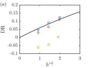
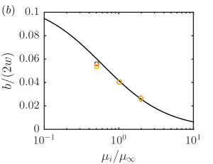
Figure 3: Drag reduction as a function of ($a$) the slip length and ($b$) slip length normalised by the pitch as a function of viscosity ratio. Symbols and colours are the same as in fig. 1. In panel ($b$), the points for different $\mathrm{We}$ are almost on top of each other. Analytical relations are shown by black lines: ($a$)  Rastegari & Akhavan (2015) and ($b$)  Schönecker et al. (2014).

The waves formed on the interface at $\mathrm{We}=200$ are sufficiently large to cause roughness effects. Interface height profiles at different times are shown in fig. 4, together with amplitudes of a wave in its initial stage (fig. 4, yellow). The wave amplitude is defined as the height of the local maximum of the wave. Wave amplitudes of $a^{+}>5$ are observed and these extend outside the viscous sublayer, indicating that the surface is transitionally rough. The amplitude grows initially at an exponential rate, before it levels off. In contrast, interface fluctuations for $\mathrm{We}=100$ have small amplitudes ($a^{+}<1$) (fig. 4) and show a significantly smaller growth rate (fig. 4, blue). The exponential growth rate (fig. 4, dashed) is an indication of a linear instability. In the next section, we provide evidence of a critical-layer instability (Miles, 1957), where energy is transferred to the wave perturbation from the turbulent flow.

3.2 Conditions for phase speed and growth rate of capillary waves

We assume a small perturbation on the liquid-liquid interface of the form

$$\eta=Ae^{ik_{x}(x-ct)}\cos(k_{z}z),$$ (3)

where $z=0$ is located in the centre of the groove. As illustrated in fig. 1, $\eta$ is the height of the interface, $A$ is the initial wave amplitude, $c$ is a complex wave speed and $t$ is time. Moreover, $k_{x}=2\pi/\lambda_{x}$ and $k_{z}=2\pi/\lambda_{z}$ are streamwise and spanwise wavenumbers, respectively. The spanwise wavelength can have a maximum value of $\lambda_{z}=2w$, due to the finite width of the grooves. This value can be seen to dominate in the snapshots of fig. 2, as most waves only have one crest or one trough in the spanwise direction. We also observe from fig. 2 that streamwise wavelengths are generally similar to, or larger than, $\lambda_{z}$. This three-dimensionality implies that both spanwise and streamwise curvatures contribute to the capillary pressure of a wave,

$$\Delta p_{\mathrm{cap}}=p_{0}^{+}-p_{0}^{-}=\gamma\left(\frac{\partial^{2}}{\partial x^{2}}+\frac{\partial^{2}}{\partial z^{2}}\right)\eta=-\gamma k^{2}\eta.$$ (4)

Here, $k=\sqrt{k_{x}^{2}+k_{z}^{2}}$ and $p_{0}^{+}$ ($p_{0}^{-}$) is the pressure above (below) the interface.

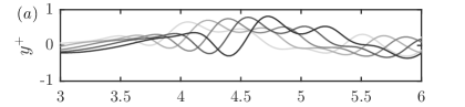
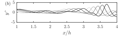
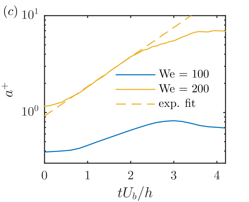
Figure 4: Instantaneous interface heights in the centerline of a groove for $\mu_{i}/\mu_{\infty}=1$: ($a$) $\mathrm{We}=100$ for $3\leq x\leq 6$ and ($b$) $\mathrm{We}=200$ for $1\leq x\leq 4$. The five profiles are separated by $\Delta t=0.2h/U_{b}$. Note the difference in vertical scale. In ($c$), the wave amplitude developing at $x/h=4.5$ in ($a$) and at $x/h=3.5$ in ($b$) are shown. The phase speeds in ($a$) and ($b$) can be estimated as $c^{+}\approx 14$ and $c^{+}\approx 10$, respectively.

Next, we consider a wall-normal velocity disturbance $v(x,y,z,t)$ on the turbulent mean flow $U(y)$ with the same waveform as $\eta$. If we neglect viscous and nonlinear effects, the amplitude $\hat{v}(y)$ is governed by the Rayleigh equation (SM, sec. S3 A),

$$\frac{1}{k^{2}}\hat{v}^{\prime\prime}-\left[1+\frac{1}{(U-c)}\frac{1}{k^{2}}U^{\prime\prime}\right]\hat{v}=0,$$ (5)

where ^′ denotes a derivative with respect to $y$. The velocity perturbation must vanish at infinity and satisfy the kinematic condition at the interface, $v/(U-c)=ik_{x}\eta$. The equation for the pressure amplitude, $\hat{p}(y)$, corresponding to eq. (5) is

$$\frac{\hat{p}}{\rho}=-i\frac{k_{x}}{k^{2}}\left[(U-c)\hat{v}^{\prime}-U^{\prime}\hat{v}\right].$$ (6)

Our aim is to find an approximate solution to the equations (4-6) in order to determine the phase speed $\Re(c)$ (real part) and growth rate $\Im(k_{x}c)$ (imaginary part) of the interface perturbation (3).

Miles (1957) formulated a similar set of equations for describing wind-induced water waves, where gravity – instead of capillarity – balances fluid pressure. He suggested the following approximate solution for $v$:

$$v=ik_{x}\eta(U-c)e^{-ky},\qquad y\geq 0.$$ (7)

This expression, which satisfies the boundary conditions at $y\rightarrow\infty$, implies that $1/k$ is the relevant length scale over which $v$ decreases. The assumption of exponential decay can also be used in the grooves:

$$v=-ik_{x}c\eta e^{ky},\qquad y<0.$$ (8)

Here, we have assumed that the grooves are sufficiently deep such that the velocity perturbation is nearly zero at the bottom of the groove. With a depth $w$, $kw>k_{z}w\geq(2\pi/(2w))w=\pi$, and, since $e^{-\pi}\ll 1$, the assumption is valid for our configuration. We have also neglected $U$ and its derivative inside the groove. Inserting (8) into (6) results in the following expression for the pressure immediately below the interface ($y\rightarrow 0^{-}$):

$$p_{0}^{-}=\rho\frac{k_{x}^{2}}{k}c^{2}\eta.$$ (9)

Similarly, by inserting (7) into (6) the pressure just above the interface is

$$p_{0}^{+}=(\alpha+i\beta)\rho U_{1}^{2}\frac{k_{x}^{2}}{k}\eta,$$ (10)

where $\alpha$ and $\beta$ are real constants and $U_{1}$ is an arbitrary reference velocity. It is shown in SM (sec. S3 C) that the parameter $\alpha$ can be decomposed into two parts, $\alpha=\alpha_{1}+\alpha_{2}$, where $\alpha_{1}$ corresponds to eq. (9) and $\alpha_{2}$ incorporates the remaining contributions from the slip velocity and the shear. Using this decomposition and inserting (9) and (10) into (4), we obtain (SM, sec. S3 D),

$$c=c_{w}\left(1+\frac{1}{4}(\alpha_{2}+i\beta)\frac{U_{1}^{2}}{c_{w}^{2}}+\dots\right).$$ (11)

Here $c_{w}=\sqrt{\gamma k^{3}/(2\rho k_{x}^{2})}$ is the free phase speed, i.e. the speed of a capillary wave without forcing from the overlying flow.

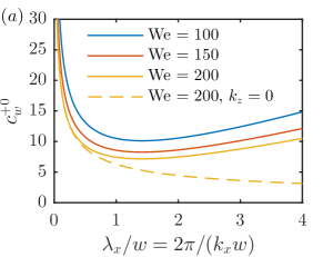
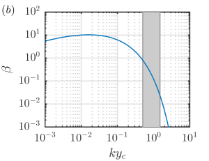
Figure 5: ($a$) The free phase speed $c^{+0}_{w}$ for $\mathrm{We}=\{100,150,200\}$ when $k_{z}=\pi/w$ (i.e. $\lambda_{z}/w=2$). For $\mathrm{We}=200$, the phase speed of a two-dimensional wave ($k_{z}=0$) is also shown. ($b$) The growth rate coefficient $\beta$ versus $ky_{c}$, showing a fast decrease in $\beta$ for $ky_{c}\gtrsim 1$.

The free phase speed is shown in fig. 5 (in nominal wall units) as a function of $\lambda_{x}/w$ for $\mathrm{We}=\{100,150,200\}$. We note that two-dimensional capillary waves ($k_{z}=0$) have a phase speed that monotonically decreases with $\lambda_{x}$. However, for LIS, there is a minimum phase speed due to the finite spanwise wavelength. This minimum is approximately (for the analytical expression see SM, sec. S3 D)

$$c_{w,\mathrm{min}}^{+}\approx\sqrt{\frac{\pi}{\mathrm{We}^{+}w^{+}}}.$$ (12)

For $\mathrm{We}=200$ (and $\mu_{i}/\mu_{\infty}=1$)¸ $c_{w,\mathrm{min}}^{+}=7.0$, which is slightly lower than the phase speed of the wave shown in fig. 4. One may use $c^{+}_{w,\min}$ as a lower bound of the actual phase speed of capillary waves on LIS.

We now turn our attention to the imaginary part of (11) to approximate the growth rate of the instability. As shown by Miles (1957) – and repeated in the SM (sec S3 E) – one may integrate the Rayleigh equation and evaluate the pressure equation (6) at the interface to find

$$\beta=-\pi\left|\frac{v_{c}}{k_{x}\eta U_{1}}\right|^{2}\frac{1}{k}\frac{U_{c}^{\prime\prime}}{U_{c}^{\prime}},$$ (13)

where the subscript $c$ denotes values at the position of the critical layer $y_{c}$. In order for an infinitesimal wave to have a positive growth rate, i.e. $\beta>0$, a first requirement is that $U^{\prime\prime}_{c}<0$, i.e. negative curvature at the critical layer. This is satisfied if the critical layer is outside of the viscous sublayer.

A second requirement for $\beta>0$ is that $v_{c}$ in eq. (13) is non-zero at the critical layer. The approximate solution of $v$ in eq. (7) implies, however, that $v$ is zero at the critical layer. As shown in SM (sec. 3 E), one may transform the condition for positive growth rate to an integral form to estimate $v$ in the vicinity of the critical layer. By further assuming a logarithmic mean velocity profile and setting the reference velocity to $U_{1}=u_{\tau}/\kappa$ (where $\kappa$ is the von Kármán constant), one may evaluate the expression for $\beta$ (as a function of $ky_{c}$), and obtain what is shown in fig. 5.

We observe from fig. 5 that, when $ky_{c}>3/2$, then $\beta<0.02$, which results in very slow-growing waves, whereas when $ky_{c}<1/2$, we have $\beta>0.8$, resulting in a factor 40 or more faster growth. The grey region in fig. 5 marks the range $1/2<ky_{c}<3/2$ where there is a transition from low to high growth rates. Now, since $k>k_{z}$ and the upper limit of $\lambda_{z}$ is $2w$, we may formulate bounds for the position of the critical layer. When

$$y_{c}^{+}\lesssim\frac{1}{2}\frac{w^{+}}{\pi},$$ (14)

the growth rate can be expected to be significant, in contrast to when

$$y_{c}^{+}\gtrsim\frac{3}{2}\frac{w^{+}}{\pi},$$ (15)

for which the growth is negligible.

Equations (12), (14) and (15) provide relationships between $\mathrm{We}^{+},w^{+}$ and $c_{w,\min}^{+},y_{c,\max}^{+}$ that can be confirmed by our simulations. Equation (12) states that a large $\mathrm{We}^{+}$ and/or $w^{+}$ give a small phase speed. This is observed qualitatively by following the travelling waves on the interface in fig. 4(a,b). More quantitatively, the space-time correlations of the interface height for $\mathrm{We}=100$ and $\mathrm{We}=200$ give $c^{+}=15.1$ and $c^{+}=10.5$, respectively (SM fig. S8).

Compared to $\mathrm{We}=100$, the lower phase speed for $\mathrm{We}=200$ results in a lower position of the critical layer. When the height of the critical layer approaches the interface and satisfies eq. (14), the growth rate coefficient $\beta$ of the waves (eq. 13) is large. This is confirmed by our simulations, where we observe in fig. 4 that both the growth rate and interface amplitudes are larger for $\mathrm{We}=200$ compared to $\mathrm{We}=100$.

We use an inviscid model here to get a tractable analytical solution, and to illustrate the important physics involved. It has been shown that the effect of introducing viscosity on capillary waves with relevant wavenumbers would be a slight damping (Jeng et al., 1998). However, it is possible that viscosity influences the velocity induced by the waves deep inside the grooves to a higher extent.

3.3 Implications for the design of LIS

The conditions (12), (14) and (15) can be used as design criteria for LIS. One may expect a high-performing LIS by choosing a groove width and a surface tension of the infused liquid such that – for relevant friction Reynolds numbers – the design falls within the smooth region of fig. 1. This region is defined by $(\mathrm{We}^{+},w^{+})$, where $y^{+}_{c}\geq 1.5w^{+}/\pi$, and thus from eq. (15) very small growth rates of capillary waves are predicted. Conversely, the rough region in fig. 1 shows $(\mathrm{We}^{+},w^{+})$, where $y^{+}_{c}\leq 0.5w^{+}/\pi$, and therefore waves will amplify rapidly. Here, we may expect either a very low-performing LIS or even a drag-increasing LIS due to roughness effects. In between the smooth and rough domains, we show in fig. 1 a transitional region (grey), which corresponds to $0.5w^{+}/\pi\leq y^{+}_{c}\leq 1.5w^{+}/\pi$. Here, we cannot predict if the resulting waves induce roughness effects using our analytical approach. It should be mentioned that the boundaries of the transitional region in fig. 1 are determined in three steps: (i) given $w^{+}$, determine $y^{+}_{c}$ from (14) (lower boundary) or (15) (upper boundary); (ii) given $y^{+}_{c}$, determine $c^{+}$ (phase speed) from $U^{+}(y^{+}_{c})=c^{+}$, where $U^{+}(y)$ is a turbulent mean profile of a smooth wall; and finally (iii) given $c^{+}$, assume $c^{+}\approx c^{+0}_{w,\min}$ and determine $\mathrm{We}^{+}$ from (12) (or the exact coefficient of (12) given in the SM).

Figure 1 also shows scaling laws between smooth and rough regions. For small $w^{+}$ (and thus $y_{c}^{+}$), we may assume that the critical-layer velocity is $U_{c}^{+}\approx y_{c}^{+}$. This is acceptable right above the viscous sublayer where the mean flow has some curvature. Then eq. (12) gives that the height of the lowest critical layer is $y_{c}^{+}\approx\sqrt{\pi/(\mathrm{We}^{+}w^{+})}$. By assuming that $y_{c}^{+}\sim w^{+}/\pi$, we obtain

$$w^{+}\sim(\mathrm{We}^{+})^{-1/3},$$ (16)

which is shown with dashed line in fig. 1. It is observed that this asymptotic relation represent a reasonable scaling law for $w^{+}\lesssim 20$.

For larger $w^{+}$, away from the viscous sublayer, we assume $U^{+}=(1/\kappa)\log(y^{+})+B$, where $B$ is a constant. This gives a nonlinear relation

$$1/(\sqrt{\mathrm{We}^{+}w^{+}})\sim(1/\kappa)\log(w^{+}/\pi).$$ (17)

This curve is shown in fig.  1 with a dashed-dotted line, and provides a scaling of the neutral curve for $w^{+}\gtrsim 30$.

The scaling laws illustrate that, when $w^{+}$ increases, there needs to be rapid decrease of $\mathrm{We}^{+}$ to remain in the smooth region. For example, for $w^{+}\approx 70$, we need $\mathrm{We}^{+}\approx 3\cdot 10^{-4}$, which corresponds to $\mathrm{We}\approx 10$. This is relevant for drag reduction, since the width of the grooves should be maximised for a given surface tension to optimise $\mathrm{DR}$ (see fig. 3), but without entering the rough zone in fig. 1. Note that for a fixed geometry, increasing the flow speed, and thereby $u_{\tau}$, increases both $\mathrm{We}^{+}$ and $w^{+}$, so that the design needs to be made for the largest flow speed to which the surface is exposed.

Finally, in fig. 1, the values of our numerical simulations are shown with symbols. These also include more extreme Weber numbers, $\mathrm{We}=50$ and $\mathrm{We}=400$ (using $\mu_{i}/\mu_{\infty}=1$), which resulted in a drag reduction of $9.3\%$ and $-15\%$, respectively, confirming the trend of the other simulations. In addition to the simulations at $w^{+0}=18$, we also show points (circles) for larger grooves of width $w^{+0}=36$ (also using $\mu_{i}/\mu_{\infty}=1$). For these grooves, there was a drag reduction by $18\%$ for $\mathrm{We}=25$ (purple circle) and $17\%$ for $\mathrm{We}=50$ (green circle), whereas for $\mathrm{We}=100$ (blue circle), the drag reduction was lowered to $2\%$ and we observed large waves. This implies that the growth rate rapidly increases between the last two cases as they fall in the transitional zone in fig. 1.

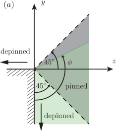
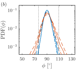
Figure 6: ($a$) If $\theta<\phi<\theta+90\degree$, the contact line remains pinned according to Gibbs’ criterion (grey area). This is illustrated for $\theta=45\degree$. If $\phi$ is outside this range, the contact line depins, and moves in the direction indicated by the arrows. ($b$) The PDF of $\phi$ from simulations for the pinned cases with $w^{+0}=18$, $\theta=45\degree$, $\mu_{i}/\mu_{\infty}=0.5$ (), $\mu_{i}/\mu_{\infty}=1$ () and $\mu_{i}/\mu_{\infty}=2$ () and the Weber numbers $\mathrm{We}=100$ (blue) and $\mathrm{We}=150$ (red). The boundaries of the interval corresponding to a probability of 95% for the widest PDF are also shown ().

3.4 Contact line depinning

The capillary waves modify the contact angle between the interface and the wall, and may potentially result in a depinning of the interface from the corners of the ridges. According to Gibbs’ criterion, which is a purely geometrical criterion, the interface remains pinned if $\theta<\phi<90\degree+\theta$, where $\phi$ is the angle the interface makes to the inner wall of the groove. The lower limit is the limit for when the contact line moves into the groove, while the upper is the limit for when it moves on top of the ridge (Gibbs, 1906). This is illustrated in fig. 6. In contrast to the cases $\mathrm{We}=100$ or $150$ (fig. 2), we observed that for $\mathrm{We}=200$ the interface depinned occasionally due to the waves on the interface.

The measured probability density functions (PDF) of $\phi$ for $\mathrm{We}=100$ and $150$ with $\theta=45\degree$ are plotted in fig. 6 for all three viscosity ratios. Since the contact line was observed to remain pinned for these parameters, the PDF are independent of $\theta$ and can be used to predict limits for the contact angle. It can be noted that the PDF for all parameters shown are centred around $\phi=90\degree$ and that $\phi$ is unlikely to reach below $70\degree$ or above $110\degree$. The interval between these values corresponds to a probability of more than 95% for the widest PDF. The standard deviation of $\phi$ decreases with $\mu_{i}/\mu_{\infty}$ and increases with $\mathrm{We}$, as is indicated by the width of the PDF. This is to be expected, since the dissipation rate increases with the viscosity and the restoring force of surface tension becomes weaker with increasing $\mathrm{We}$.

A restoring force for the contact line also comes from mass conservation. If the contact line occasionally does depin into the groove on one position, it will be raised elsewhere. Based on this observation and the statistics in fig. 6, depinning is not the main failure mode of LIS for the geometry chosen in this study. Depinning is, however, expected to be important for a LIS with grooves of finite length.

4 Conclusions

We have explored the behaviour of LIS in a turbulent channel flow with square longitudinal grooves for $\mathrm{Re}_{\tau}\approx 180$. By allowing the interface and the contact line to move, we could investigate the unconstrained motion of the interface. For a fixed groove width, we found a rapid increase in drag of LIS above a certain Weber number due to the appearance of large capillary waves. The generation mechanism of these waves was elucidated using the theory developed by Miles (1957). The limit for when these waves act as roughness is set by the width of the grooves $w^{+}$ and the Weber number $\mathrm{We}^{+}$, as illustrated in fig. 1. It should also be noted that these non-dimensional parameters depend on the flow speed. Using an analytical analysis, we have provided scaling laws and design criteria for robust drag-reducing LIS. Specifically, the relations show how to achieve a balance between large groove widths (enhancing drag reduction) and high surface tension of the infused liquid (enhancing stability) for different flow speeds.

[Acknowledgements]This work was supported by SSF, the Swedish Foundation for Strategic Research (Future Leaders grant FFL15:0001). Simulations were performed on resources provided by the Swedish National Infrastructure of Computing (SNIC).

[Declaration of interests]The authors report no conflict of interest.

[Supplementary data]Supplementary material are available at
https://doi.org/10.1017/jfm.2021.241.

References

- Aniszewski et al. (2021) Aniszewski, W., Arrufat, T., Crialesi-Esposito, M., Dabiri, S., Fuster, D., Ling, Y., Lu, J., Malan, L., Pal, S., Scardovelli, R., Tryggvason, G., Yecko, P. & Zaleski, S. 2021 PArallel, Robust, Interface Simulator (PARIS). Comput. Phys. Commun. 263, 107849.
- Arenas et al. (2019) Arenas, I., García, E., Fu, M. K., Orlandi, P., Hultmark, M. & Leonardi, S. 2019 Comparison between super-hydrophobic, liquid infused and rough surfaces: a direct numerical simulation study. J. Fluid Mech. 869, 500–525.
- Arrufat et al. (2021) Arrufat, T., Crialesi-Esposito, M., Fuster, D., Ling, Y., Malan, L., Pal, S., Scardovelli, R., Tryggvason, G. & Zaleski, S. 2021 A mass-momentum consistent, volume-of-fluid method for incompressible flow on staggered grids. Comput. Fluids 215, 104785.
- Boomkamp & Miesen (1996) Boomkamp, P. A. M. & Miesen, R. H. M. 1996 Classification of instabilities in parallel two-phase flow. Int. J. Multiph. Flow 22, 67–88.
- Cartagena et al. (2018) Cartagena, E. J. G., Arenas, I., Bernardini, M. & Leonardi, S. 2018 Dependence of the drag over super hydrophobic and liquid infused surfaces on the textured surface and weber number. Flow Turbul. Combust. 100 (4), 945–960.
- Epstein et al. (2012) Epstein, A. K., Wong, T., Belisle, R. A., Boggs, E. M. & Aizenberg, J. 2012 Liquid-infused structured surfaces with exceptional anti-biofouling performance. Proc. Natl. Acad. Sci. 109 (33), 13182–13187.
- Fu et al. (2017) Fu, M. K., Arenas, I., Leonardi, S. & Hultmark, M. 2017 Liquid-infused surfaces as a passive method of turbulent drag reduction. J. Fluid Mech. 824, 688–700.
- Fu et al. (2019) Fu, M. K., Chen, T., Arnold, C. B. & Hultmark, M. 2019 Experimental investigations of liquid-infused surface robustness under turbulent flow. Exp. Fluids 60 (6), 100.
- Gibbs (1906) Gibbs, J. W. 1906 The scientific papers of J. Willard Gibbs, , vol. 1. Longmans, Green and Company.
- Jeng et al. (1998) Jeng, U., Esibov, L., Crow, L. & Steyerl, A. 1998 Viscosity effect on capillary waves at liquid interfaces. J. Phys. Condens. Matter 10 (23), 4955–4962.
- Kim et al. (2012) Kim, P., Wong, T., Alvarenga, J., Kreder, M. J., Adorno-Martinez, W. E. & Aizenberg, J. 2012 Liquid-infused nanostructured surfaces with extreme anti-ice and anti-frost performance. ACS nano 6 (8), 6569–6577.
- Legendre & Maglio (2015) Legendre, D. & Maglio, M. 2015 Comparison between numerical models for the simulation of moving contact lines. Comput. Fluids 113, 2–13.
- Ling et al. (2017) Ling, H., Katz, J., Fu, M. & Hultmark, M. 2017 Effect of reynolds number and saturation level on gas diffusion in and out of a superhydrophobic surface. Phys. Rev. Fluids 2 (12), 124005.
- Miles (1957) Miles, J. W. 1957 On the generation of surface waves by shear flows. J. Fluid Mech. 3 (2), 185–204.
- Rastegari & Akhavan (2015) Rastegari, A. & Akhavan, R. 2015 On the mechanism of turbulent drag reduction with super-hydrophobic surfaces. J. Fluid Mech. 773, R4.
- Schönecker et al. (2014) Schönecker, C., Baier, T. & Hardt, S. 2014 Influence of the enclosed fluid on the flow over a microstructured surface in the cassie state. J. Fluid Mech. 740, 168–195.
- Seo et al. (2018) Seo, J., García-Mayoral, R. & Mani, A. 2018 Turbulent flows over superhydrophobic surfaces: flow-induced capillary waves, and robustness of air–water interfaces. J. Fluid Mech. 835, 45–85.
- Van Buren & Smits (2017) Van Buren, T. & Smits, A. J. 2017 Substantial drag reduction in turbulent flow using liquid-infused surfaces. J. Fluid Mech. 827, 448–456.
- Wang et al. (2015) Wang, P., Lu, Z. & Zhang, D. 2015 Slippery liquid-infused porous surfaces fabricated on aluminum as a barrier to corrosion induced by sulfate reducing bacteria. Corros. Sci. 93, 159–166.
- Wexler et al. (2015) Wexler, J. S., Jacobi, I. & Stone, H. A. 2015 Shear-driven failure of liquid-infused surfaces. Phys. Rev. Lett. 114 (16), 168301.
- Weymouth & Yue (2010) Weymouth, G. D. & Yue, Dick K.-P. 2010 Conservative volume-of-fluid method for free-surface simulations on cartesian-grids. J. Comput. Phys. 229 (8), 2853–2865.
- Wong et al. (2011) Wong, T., Kang, S. H., Tang, S. K. Y., Smythe, E. J., Hatton, B. D., Grinthal, A. & Aizenberg, J. 2011 Bioinspired self-repairing slippery surfaces with pressure-stable omniphobicity. Nature 477 (7365), 443–447.