Spectral Analysis for Preconditioning of Multi-dimensional Riesz Fractional Diffusion Equations

Abstract

In this paper, we analyze the spectra of the preconditioned matrices arising from discretized multi-dimensional Riesz spatial fractional diffusion equations. The finite difference method is employed to approximate the multi-dimensional Riesz fractional derivatives, which will generate symmetric positive definite ill-conditioned multi-level Toeplitz matrices. The preconditioned conjugate gradient method with a preconditioner based on the sine transform is employed to solve the resulting linear system. Theoretically, we prove that the spectra of the preconditioned matrices are uniformly bounded in the open interval $(1/2,3/2)$ and thus the preconditioned conjugate gradient method converges linearly. The proposed method can be extended to multi-level Toeplitz matrices generated by functions with zeros of fractional order. Our theoretical results fill in a vacancy in the literature. Numerical examples are presented to demonstrate our new theoretical results in the literature and show the convergence performance of the proposed preconditioner that is better than other existing preconditioners.

65F08, 65M10, 65N99

1 Introduction

In this paper, we study the preconditioning technique for the following multi-dimensional Riesz fractional diffusion equations

(1) $$-\sum\limits_{i=1}^{m}d_{i}\frac{\partial^{\alpha_{i}}u(\bf x)}{\partial|x_{i}|^{\alpha_{i}}}=y({\bf x}),\quad{\bf x}\in{\Omega}=\prod_{i=1}^{m}[a_{i},b_{i}]\subset{\mathbb{R}}^{m},$$

subject to the boundary condition

$$u({\bf x})=0,\ {\bf x}\in\partial\Omega,$$

where $d_{i}>0$ for $i=1,\dots,m$, ${\bf x}=(x_{1},\dots,x_{m})\in{\mathbb{R}}^{m}$, $y({\bf x}):{\mathbb{R}}^{m}\mapsto{\mathbb{R}}$ is the source term, and $\frac{\partial^{\alpha_{i}}u({\bf x})}{\partial|x_{i}|^{\alpha_{i}}}$ is the Riesz fractional derivative of ${\alpha_{i}}\in(1,2)$ with respect to $x_{i}$ defined by

(2) $$\frac{\partial^{\alpha_{i}}u({\bf x})}{\partial|x_{i}|^{\alpha_{i}}}=c(\alpha_{i})\left({}_{a_{i}}D_{x_{i}}^{\alpha_{i}}u({\bf x})+_{x_{i}}D_{b_{i}}^{\alpha_{i}}u({\bf x})\right),\ c(\alpha_{i})=\frac{-1}{2\cos(\frac{\alpha_{i}\pi}{2})}>0.$$

The above left and right Riemann-Liouville (RL) fractional derivatives are defined by

(3) $${}_{a_{i}}{\rm D}_{x_{i}}^{\alpha_{i}}u({\bf x})=\frac{1}{\Gamma(2-{\alpha_{i}})}\frac{\partial^{2}}{\partial x_{i}^{2}}\int_{a_{i}}^{x_{i}}\frac{u(x_{1},x_{2},\dots,x_{i-1},\xi,x_{i+1},\dots,x_{m})}{(x_{i}-\xi)^{\alpha_{i}-1}}{\rm d}\xi,$$

(4) $$_{x_{i}}{\rm D}_{b_{i}}^{\alpha_{i}}u({\bf x})=\frac{1}{\Gamma(2-{\alpha_{i}})}\frac{\partial^{2}}{\partial x_{i}^{2}}\int_{x_{i}}^{b_{i}}\frac{u(x_{1},x_{2},\dots,x_{i-1},\xi,x_{i+1},\dots,x_{m})}{(\xi-x_{i})^{\alpha_{i}-1}}{\rm d}\xi,$$

respectively, where ${\Gamma(\cdot)}$ is the gamma function.

Fractional calculus has received an increasing interest since its applications involve various fields including physics, chemistry, engineering; see [11, 17, 18, 28]. The Riesz fractional derivative, which derives from the kinetic of chaotic dynamics [31], is generalized as one of the most popular fractional calculus. Recently, the study of the Riesz fractional derivative has been urgent and significant as it can be applied to lattice model with long-range interactions [12], nonlocal dynamics [36], and so on.

After discretization by the finite difference method, the resulting coefficient matrix of the above multi-dimensional Riesz fractional derivative in (1) is a dense multi-level Toeplitz matrix; i.e., each block has a Toeplitz structure. It is interesting to note that such multi-level Toeplitz matrix can be generated by a continuous real-valued even function which is nonnegative defined on the interval $[-\pi,\pi]$ [26]. Moreover, the diagonal entries are the Fourier coefficients of the generating function with ${\alpha}$-th order zero at the origin ($1<\alpha<2$). Hence, the condition number of the discretized linear system is unbounded as the matrix size tends to infinity. More precisely, the condition number grows as $n^{\alpha}$, where $n$ denotes the matrix size; see [7, 6, 33]. Therefore, the resulting linear system arising from (1) is ill-conditioned and thus the conjugate gradient (CG) method for this system converges slowly.

In order to speed up the convergence of the CG method, preconditioning techniques have been proposed and developed for ill-conditioned Toeplitz systems. For examples, banded Toeplitz preconditioners [7, 3] were proposed to handle ill-conditioned Toeplitz linear systems where the generating functions of Toeplitz matrices have zeros of even order. When these banded Toeplitz preconditioners are applied to Toeplitz matrices generated by functions with ${\alpha}$-th order zero at the origin ($1<\alpha<2$), the condition numbers of these preconditioned systems are not uniformly bounded.

Besides, several strategies have been exploited for the ill-conditioned Toeplitz systems, such as $\tau$-preconditioners (which can be diagonalized by the discrete sine transform matrix) [4, 2, 9, 34], circulant preconditioners [29, 10, 30, 24], and multigrid methods [15, 16, 8, 35, 3, 32]. These approaches can significantly speed up the convergence of iterative methods for solving Toeplitz systems where their generating functions have an ${\alpha}$-th order zero at the origin ($1<\alpha<2$). However, the linear convergence of these methods cannot be theoretically confirmed for solving such Toeplitz systems. Lately, some efficient preconditioners are developed to solve linear systems arising from fractional diffusion equations; see [13, 21, 14, 1, 23]. Nevertheless, from the theoretical point of view, the spectra of these preconditioned matrices are not shown to be bounded independent of the matrix sizes and hence the linear convergence cannot be guaranteed.

In order to tackle this theoretical problem, Noutsos, Serra and Vassalos [25] exploited a multiple step preconditioning and applied to the case where the generating functions of coefficient matrices have fractional order zeros. In their method, they proposed a new $\tau$-preconditioner that is constructed from the generating function of the given Toeplitz matrix. Numerical results were shown that their method worked very well for the Toeplitz matrices whose generating functions have fractional order zeros. Theoretically, they have proved that the largest eigenvalue of the preconditioned matrix has an upper bound independent of the matrix size. Nevertheless, it is still unclear whether the smallest eigenvalue of the preconditioned matrix is bounded below away from zero; see the remark in [25].

The main aim of this paper is to conduct the spectral analysis of the $\tau$-preconditioner for the ill-conditioned multi-level Toeplitz system arising from the discretized Riesz fractional derivatives. Theoretically, we prove that the spectra of the $\tau$-preconditioned matrices are uniformly bounded in the open interval $(1/2,3/2)$ and thus the preconditioned CG (PCG) method converges linearly. Furthermore, the proposed method can be extended to multi-level Toeplitz matrices generated by functions with zeros of fractional order. Similarly, we show that the spectra of these preconditioned multi-level Toeplitz matrices are uniformly bounded. Numerical examples are presented to verify our new theoretical results in the literature and show the good performance of the proposed preconditioner.

The outline of the rest paper is as follows. In Section 2, multi-level Toeplitz matrices are generated. In Section 3, the preconditioner is proposed and developed. In Section 4, the spectral analysis of the preconditioned matrix is discussed. In Section 5, a new preconditioning technique for multi-level Toeplitz matrices is studied. Numerical experiments are given in Section 6 to show the performance of the proposed preconditioner. Finally, some concluding remarks are given in Section 7.

2 Multi-level Toeplitz matrices

A matrix, whose entries are constant along the diagonals with the following form

(5) $$T_{n}=\left[\begin{array}[]{ccccc}t_{0}&t_{-1}&\dots&t_{2-n}&t_{1-n}\\ t_{1}&t_{0}&t_{-1}&\dots&t_{2-n}\\ \vdots&t_{1}&t_{0}&\ddots&\vdots\\ t_{n-2}&\ddots&\ddots&\ddots&t_{-1}\\ t_{n-1}&t_{n-2}&\dots&t_{1}&t_{0}\\ \end{array}\right],$$

is called a Toeplitz matrix. Assume that the diagonals $\{t_{k}\}_{k=1-n}^{n-1}$ of $T_{n}$ are the Fourier coefficients of a function $f$; i.e.,

$$t_{k}=\frac{1}{2\pi}\int_{-\pi}^{\pi}f(\theta)e^{-{\bf i}k\theta}d\theta,$$

then the function $f$ is called the generating function of $T_{n}$. Generally, denote $T_{n}=T_{n}(f)$ to emphasize that an $n\times n$ Toeplitz matrix $T_{n}$ is generated by $f$. Moreover, if the generating function is real and even, then $T_{n}$ is real symmetric for all $n$.

Let ${{\boldsymbol{\theta}}}=(\theta_{1},\theta_{2},\dots,\theta_{m})\in[-\pi,\pi]^{m}$, $f({\boldsymbol{\theta}})=f(\theta_{1},\dots,\theta_{m})\in L^{1}([-\pi,\pi]^{m})$. The matrix generated by function $f({{\boldsymbol{\theta}}})$ is an $m$-level Toeplitz matrix with Toeplitz structure on each level. Let $n_{i}$ for $i=1,2,\dots,m$ be positive integers. Denote $N=\prod\limits_{i=1}^{m}n_{i}$. Then an $m$-level Toeplitz matrix with the size $N\times N$ is a block Toeplitz matrix with Toeplitz block, and its form is

(6) $$T_{N}^{m}=\left[\begin{array}[]{cccc}T_{0}^{m-1}&T_{-1}^{m-1}&\cdots&T_{1-{n_{m}}}^{m-1}\\ T_{1}^{m-1}&T_{0}^{m-1}&\ddots&\vdots\\ \vdots&\ddots&\ddots&T_{-1}^{m-1}\\ T_{n_{m}-1}^{m-1}&\cdots&T_{1}^{m-1}&T_{0}^{m-1}\end{array}\right],$$

where each block $T_{j}^{m-1}$ for $j=0,\dots,n_{m}-1$ is an $(m-1)$-level block Toeplitz of size $(n_{1}\cdots n_{m-1})\times(n_{1}\cdots n_{m-1})$ with $(m-2)$-level Toeplitz block of size $(n_{1}\cdots n_{m-2})\times(n_{1}\cdots n_{m-2})$, and so on. Let $(j_{1},\dots,j_{m})\in{{\mathbb{Z}}}^{m}$ be a multi-index. Then the coefficients of $T_{N}^{m}$ can be obtained by [27]

(7) $$t_{j_{1},j_{2},\dots,j_{m}}=\frac{1}{(2\pi)^{m}}\int_{[-\pi,\pi]^{m}}f({{\boldsymbol{\theta}}})e^{-{\bf i}\sum\limits_{i=1}^{m}\theta_{i}j_{i}}d{{\boldsymbol{\theta}}}.$$

2.1 Discretized 1D Riesz fractional derivative

Firstly, we consider the one dimensional case. Let $n$ be the partition of the interval $[a,b]$. We define a uniform spatial partition

$$h=\frac{b-a}{n+1},\quad\eta_{j}=a+jh,\quad{\rm for}\ j=0,1,\dots,n+1.$$

Then the following shifted Grünwald-Letnikov formula is exploited to approximate the left- and right- RL fractional derivatives at grid point $\eta_{j}$,

(8) $$_{a}D_{x}^{\alpha}u(\eta_{j})=\frac{1}{h^{\alpha}}\sum_{k=0}^{j+1}g_{k}^{(\alpha)}u(\eta_{j-k+1})+{\mathcal{O}}(h),$$

(9) $$_{x}D_{b}^{\alpha}u(\eta_{j})=\frac{1}{h^{\alpha}}\sum_{k=0}^{n-j+2}g_{k}^{(\alpha)}u(\eta_{j+k-1})+{\mathcal{O}}(h),$$

where the coefficients $g_{k}^{(\alpha)}$ are defined by

(10) $$g_{0}^{(\alpha)}=1,\quad g_{k}^{(\alpha)}=\left(1-\frac{\alpha+1}{k}\right)g_{k-1}^{(\alpha)},\quad{\rm for}\ k\geq 1.$$

It can be shown that the coefficients $g_{k}^{(\alpha)}$ defined above have the following properties.

Lemma 2.1.

(see [22]) For ${\alpha}\in(1,2)$, the coefficients $g_{k}^{(\alpha)}$, $k=0,1,\dots$, satisfy

$$\left\{\begin{aligned} &g_{0}^{(\alpha)}=1,\ g_{1}^{(\alpha)}=-{\alpha}<0,\ g_{2}^{(\alpha)}>g_{3}^{(\alpha)}>\cdots>0,\\ &\sum\limits_{k=0}^{\infty}g_{k}^{(\alpha)}=0,\ \sum\limits_{k=0}^{n}g_{k}^{(\alpha)}<0,\ {\rm for}\ n\geq 1.\end{aligned}\right.$$

By applying (8) and (9) to the model equation (1), we obtain

(11) $$-d\frac{c(\alpha)}{h^{\alpha}}\left(\sum_{k=0}^{j+1}g_{k}^{(\alpha)}u(\eta_{j-k+1})+\sum_{k=0}^{n-j+2}g_{k}^{(\alpha)}u(\eta_{j+k-1})\right)=y(\eta_{j})+{\mathcal{O}}(h).$$

Defining $u_{j}$ as the numerical approximation of $u(\eta_{j})$, setting $y_{j}=y(\eta_{j})$, and omitting the small term ${\mathcal{O}}(h)$, the finite difference scheme for solving (1) is constructed as follows

(12) $$-d\frac{c(\alpha)}{h^{\alpha}}\left(\sum_{k=0}^{j+1}g_{k}^{(\alpha)}u_{j-k+1}+\sum_{k=0}^{n-j+2}g_{k}^{(\alpha)}u_{j+k-1}\right)=y_{j},\quad{\rm for}\ j=1,\dots,n.$$

Let $u=[u_{1},\dots,u_{n}]^{\intercal}$, $y=[y_{1},\dots,y_{n}]^{\intercal}$. Then, the numerical scheme (12) can be simplified as the following matrix-vector form

(13) $$A_{n}u=y,$$

with $A_{n}=wG_{n}^{(\alpha)}$, where $w=\frac{dc(\alpha)}{h^{\alpha}}>0$ and

(14) $${\small G_{n}^{(\alpha)}=-\left[\begin{array}[]{cccccc}2g_{1}^{(\alpha)}&g_{0}^{(\alpha)}+g_{2}^{(\alpha)}&g_{3}^{(\alpha)}&\ddots&g_{n-1}^{(\alpha)}&g_{n}^{(\alpha)}\\ g_{0}^{(\alpha)}+g_{2}^{(\alpha)}&2g_{1}^{(\alpha)}&g_{0}^{(\alpha)}+g_{2}^{(\alpha)}&g_{3}^{(\alpha)}&\ddots&g_{n-1}^{(\alpha)}\\ \vdots&g_{0}^{(\alpha)}+g_{2}^{(\alpha)}&2g_{1}^{(\alpha)}&\ddots&\ddots&\vdots\\ \vdots&\ddots&\ddots&\ddots&\ddots&g_{3}^{(\alpha)}\\ g_{n-1}^{(\alpha)}&\ddots&\ddots&\ddots&2g_{1}^{(\alpha)}&g_{0}^{(\alpha)}+g_{2}^{(\alpha)}\\ g_{n}^{(\alpha)}&g_{n-1}^{(\alpha)}&\cdots&\cdots&g_{0}^{(\alpha)}+g_{2}^{(\alpha)}&2g_{1}^{(\alpha)}\\ \end{array}\right].}$$

It is evident that the matrix $G_{n}^{(\alpha)}$ is a symmetric Toeplitz matrix, which is generated by an integrable real-value even function defined on the interval $[-\pi,\pi]$. In the following, the generating function of matrix $G_{n}^{(\alpha)}$ will be presented.

Lemma 2.2.

(see [26]) The generating function of matrix $G_{n}^{(\alpha)}$ is

(15) $$g_{\alpha}({\theta})=\left\{\begin{array}[]{l}\vspace{1mm}-2^{\alpha+1}(\sin\frac{-{\theta}}{2})^{\alpha}\cos[\frac{\alpha}{2}(\pi+{\theta})-{\theta}],\ {\theta}\in[-\pi,0),\\ -2^{\alpha+1}(\sin\frac{{\theta}}{2})^{\alpha}\cos[\frac{\alpha}{2}(\pi-{\theta})+{\theta}],\ \ {\theta}\in[0,\pi].\end{array}\right.$$

By Lemma 2.2, the generating function of $G_{n}^{(\alpha)}$ possesses the following properties, which will be exploited to further study.

Lemma 2.3.

For any ${\alpha}\in(1,2)$, it holds that

$$\frac{1}{2}\leq\frac{|\theta|^{\alpha}}{g_{\alpha}({\theta})}\leq\frac{\pi^{2}}{-8\cos(\frac{\pi\alpha}{2})},\ where\ {\theta}\in[-\pi,\pi].$$

Proof 2.4.

We only consider the case that ${\theta}\in(0,\pi]$ as it is an even function. From Lemma 2.2, we have

$$\frac{|{\theta}|^{\alpha}}{g_{\alpha}({\theta})}=-\frac{{\theta}^{\alpha}}{2^{\alpha+1}(\sin\frac{{\theta}}{2})^{\alpha}\cos[\frac{\alpha}{2}(\pi-{\theta})+{\theta}]}.$$

Note that $1<{\alpha}<2$, it holds

$$\frac{1}{2}<\frac{{\theta}^{\alpha}}{2^{\alpha+1}(\sin\frac{{\theta}}{2})^{\alpha}}=\frac{1}{2}\frac{(\frac{{\theta}}{2})^{\alpha}}{(\sin\frac{{\theta}}{2})^{\alpha}}\leq\frac{\pi^{2}}{8},$$

and

$$1\leq-\frac{1}{\cos[\frac{\alpha}{2}(\pi-{\theta})+{\theta}]}\leq-\frac{1}{\cos(\frac{\pi\alpha}{2})}.$$

Similarly, we can derive the same conclusion for ${\theta}\in[-\pi,0)$ and the result is concluded.

In the light of the definition of the fractional order zero defined in [14], we deduce that the generating function $g_{\alpha}({\theta})$ has a zero of order ${\alpha}$ at ${\theta}=0$.

2.2 Multi-dimensional Riesz fractional derivatives

Now, we extend our investigation to the multi-dimensional cases as in (1). To obtain the discretized form of multi-dimensional Riesz fractional diffusion equations, some notations are required.

Denote $I_{k}$ be a $k\times k$ identity matrix. Let $n_{i}^{-}=\prod\limits_{j=1}^{i-1}n_{j}$ and $n_{i}^{+}=\prod\limits_{j=i+1}^{m}n_{j}$ for $i=1,2,\dots,m$, respectively. In particular, take $n_{1}^{-}=n_{m}^{+}=1$. Let $h_{i}=\frac{b_{i}-a_{i}}{n_{i}+1}$, for $i=1,\dots,m$, $\eta^{i}_{j}=a_{i}+jh_{i}$, and $y_{j_{1},j_{2},\ldots,j_{m}}=y(\eta^{1}_{j_{1}},\eta^{2}_{j_{2}},\ldots,\eta^{m}_{j_{m}})$. Denote

$${\bf u}=[u_{1,1,\ldots,1},\ldots,u_{n_{1},1,\ldots,1},u_{1,2,\ldots,1},\ldots,\ldots,u_{n_{1},n_{2},\ldots,n_{m}}]^{\intercal}\in{\mathbb{R}}^{N}$$

and

$${\bf y}=[y_{1,1,\ldots,1},\ldots,y_{n_{1},1,\ldots,1},y_{1,2,\ldots,1},\ldots,\ldots,y_{n_{1},n_{2},\ldots,n_{m}}]^{\intercal}\in{\mathbb{R}}^{N}.$$

Analogously, using the shifted Grünwald-Letnikov formula to discretize the multi-dimensional Riesz fractional diffusion equations (1), we obtain the matrix-vector form of the resulting linear system as

(16) $${\bf A}{\bf u}={\bf y},$$

where

(17) $${\bf A}=\sum_{i=1}^{m}I_{n_{i}^{-}}\otimes{A}_{n_{i}}\otimes I_{n_{i}^{+}},$$

in which ${A}_{n_{i}}=w_{i}G_{n_{i}}^{(\alpha_{i})}$, $w_{i}=\frac{d_{i}c({\alpha_{i}})}{h_{i}^{\alpha_{i}}}>0$, and $G_{n_{i}}^{(\alpha_{i})}$ is defined as in (14). Moreover, the generating function of ${\bf A}$ is as follows,

(18) $$f_{{\boldsymbol{\alpha}}}({\boldsymbol{\theta}})=\sum_{i=1}^{m}w_{i}g_{\alpha_{i}}(\theta_{i}),$$

where ${\boldsymbol{\alpha}}=(\alpha_{1},\ldots,\alpha_{m})$.

Note that the generating function $g_{\alpha_{i}}({\theta_{i}})$ is nonnegative and hence so is $f_{{\boldsymbol{\alpha}}}({{\boldsymbol{\theta}}})$, which manifests that the coefficient matrices $A_{n_{i}}$ and ${\bf A}$ are both symmetric positive definite. It is well-known that the CG method has been recognized as the most appropriate method for solving symmetric positive definite Toeplitz systems. Actually, since the generating functions have zeros, the corresponding matrices are ill-conditioned, which will slow down the convergent rate of the CG method. In order to speed up the convergent rate, the preconditioning technique is employed to solve the ill-conditioned system.

3 Sine transform based preconditioners

Let $T_{n}$ be a given symmetric Toeplitz matrix whose first column is $[t_{0},t_{1},\dots,t_{n-1}]^{\intercal}$. Then, the natural ${\tau}$ matrix ${\tau}(T_{n})$ of $T_{n}$ can be determined by the Hankel correction[4]

(19) $$\tau(T_{n})=T_{n}-H_{n},$$

where $H_{n}$ is a Hankel matrix whose entries are constants along the antidiagonals, in which the antidiagonals are given as

$$[t_{2},t_{3},\dots,t_{n-1},0,0,0,t_{n-1},\dots,t_{3},t_{2}]^{\intercal}.$$

More preciously, the entries $p_{ij}$ of ${\tau}(T_{n})$ can be generalized as

(20) $$p_{ij}=\left\{\begin{aligned} &t_{|j-i|}-t_{i+j},&&i+j<n-1,\\ &t_{|j-i|},&&i+j=n-1,n,n+1,\\ &t_{|j-i|}-t_{2n+2-(i+j)},&&{\rm otherwise}.\end{aligned}\right.$$

Notice that a ${\tau}$ matrix can be diagonalized by the sine transform matrix $S_{n}$ [5]; i.e.,

(21) $$\tau(T_{n})=S_{n}{\Lambda_{n}}S_{n},$$

where $\Lambda_{n}$ is a diagonal matrix holding all the eigenvalues of $\tau(T_{n})$ and the entries of $S_{n}$ are given by

(22) $$[S_{n}]_{j,k}=\sqrt{\frac{2}{n+1}}\sin\left(\frac{\pi jk}{n+1}\right),\ 1\leq k,j\leq n.$$

Obviously, $S_{n}$ is a symmetric orthogonal matrix, and the matrix-vector multiplication $S_{n}v$ for any vector $v$ can be computed with only ${{\mathcal{O}}}(n\log n)$ operations by the fast sine transform. Likewise, the matrix-vector product ${\tau}(T_{n})^{-1}v=S_{n}{\Lambda}_{n}^{-1}S_{n}v$ can be done in ${{\mathcal{O}}(n\log n)}$ operations. Moreover, the eigenvalues of the ${\tau}$ matrix can be determined by its first column. Thus, ${\mathcal{O}}(n)$ storage and ${\mathcal{O}}({n\log n})$ computational complexity are required for saving and computing the eigenvalues of the ${\tau}$ matrix, respectively.

Now we consider the preconditioner matrix of the linear system (13). Recalling the form of the coefficient matrix, we obtain the preconditioner as

(23) $$P_{n}={\tau}(A_{n})=w{\tau}(G^{(\alpha)}_{n}),$$

where $G^{(\alpha)}_{n}$ is the symmetric positive definite Toeplitz matrix defined in (14). For general ${\tau}$ matrix, we obtain its eigenvalues by the following lemma.

Lemma 3.1.

(see [4]) Let $T_{n}$ be a symmetric Toeplitz matrix whose first column is $[t_{0},t_{1},\dots,t_{n-1}]^{\intercal}$. Then the eigenvalues of ${\tau}(T_{n})$ can be expressed as

$${\sigma}_{j}=t_{0}+2\sum^{n-1}_{k=1}t_{k}\cos(j\zeta_{k}),\quad j=1,\ldots,n,$$

where $\zeta_{k}=\frac{\pi k}{n+1}$, $k=1,\dots,n-1$.

Lemma 3.1 provides a methodology to compute the eigenvalues of the $\tau$ matrix. Taking advantage of Lemma 3.1, the preconditioner $P_{n}$ can be verified to be positive definite in the following lemma.

Lemma 3.2.

The preconditioner $P_{n}=w{\tau}(G^{(\alpha)}_{n})$ defined in (23) is symmetric positive definite.

Proof 3.3.

The first column of $G^{(\alpha)}_{n}$ in (14) is

$$\left[-2g_{1}^{(\alpha)},-g_{0}^{(\alpha)}-g_{2}^{(\alpha)},-g_{3}^{(\alpha)},\dots,-g_{n}^{(\alpha)}\right]^{\intercal}.$$

According to Lemma 3.1, the $j$th eigenvalue of $\tau(G^{(\alpha)}_{n})$ can be expressed as

$${\delta}_{j} = -2g^{(\alpha)}_{1}-2\left(g^{(\alpha)}_{0}+g^{(\alpha)}_{2}\right)\cos\left(\frac{\pi j}{n+1}\right)-2\sum_{k=3}^{n}g^{(\alpha)}_{k}\cos\left(\frac{\pi j(k-1)}{n+1}\right)$$

$$\geq -2g^{(\alpha)}_{1}-2\left(g^{(\alpha)}_{0}+g^{(\alpha)}_{2}\right)-2\sum_{k=3}^{n}g^{(\alpha)}_{k}$$

$$= -2\sum^{n}_{k=0}g^{(\alpha)}_{k}>0.\qquad{\rm(by\,\lx@cref{creftype~refnum}{g-property})}$$

Therefore, we deduce that $\tau(G^{(\alpha)}_{n})$ is symmetric positive definite and conclude that so is $P_{n}$.

Making use of Lemma 3.2, we derive the following corollary.

Corollary 3.4.

The preconditioner $P_{n}$ defined in (23) is invertible.

Now we consider the $\tau$-preconditioner for multi-level Toeplitz matrices. Recall the coefficient matrix

$${\bf A}=\sum_{i=1}^{m}I_{n_{i}^{-}}\otimes{A}_{n_{i}}\otimes I_{n_{i}^{+}}.$$

The preconditioner matrix of the linear system (16) can be expressed as

(24) $${\bf P}=\sum_{i=1}^{m}{I}_{n_{i}^{-}}\otimes{\tau({A}_{n_{i}})}\otimes{I}_{n_{i}^{+}},$$

where ${\tau}({A}_{n_{i}})=w_{i}\tau(G_{n_{i}}^{(\alpha_{i})})$ for $i=1,\dots,m$. Denote

(25) $${A}_{i}={I}_{n_{i}^{-}}\otimes{A}_{n_{i}}\otimes{I}_{n_{i}^{+}},$$

and the corresponding $\tau$-matrix can be defined as ${\tau}_{1}({A}_{i})={I}_{n_{i}^{-}}\otimes{\tau({A}_{n_{i}})}\otimes{I}_{n_{i}^{+}}$.

Lemma 3.5.

The preconditioner ${\bf P}$ defined in (24) is symmetric positive definite.

Proof 3.6.

Let ${\Lambda}_{n_{i}}$ be a diagonal matrix holding the eigenvalues of ${\tau}({A}_{n_{i}})$. Then ${\tau}({A}_{n_{i}})=S_{n_{i}}{\Lambda_{n_{i}}}S_{n_{i}}$. Lemma 3.2 has shown that all the eigenvalues of ${\tau}(G_{n_{i}}^{(\alpha_{i})})$ are positive; that is, ${\tau}({A}_{n_{i}})$ for $i=1,2\dots,m$ are positive definite. By virtue of the properties of Kronecker product, it is easy to obtain

$${I}_{n_{i}^{-}}\otimes{\tau({A}_{n_{i}})}\otimes{I}_{n_{i}^{+}}={{\bf S}}(I_{n_{i}^{-}}\otimes{\Lambda}_{n_{i}}\otimes I_{n_{i}^{+}}){{\bf S}},$$

where ${{\bf S}}=\bigotimes\limits^{m}_{i=1}S_{n_{i}}$, which manifests that all the eigenvalues of ${\tau}_{1}(A_{i})$ are positive. As ${\bf P}$ is the summation of symmetric positive definite matrices, it follows that ${\bf P}$ is also symmetric positive definite.

4 Spectral analysis for preconditioned matrices

In this section, we discuss the spectra of the preconditioned matrices.

4.1 One dimensional case

In the following, we discuss the spectrum of ${\tau}(G^{(\alpha)}_{n})^{-1}H_{n}$, which is needed in the theoretical analysis.

First of all, we focus on the matrix ${\tau}(G^{(\alpha)}_{n})=G^{(\alpha)}_{n}-H_{n}$, where $H_{n}$ is the Hankel matrix as in (19), and $G_{n}^{(\alpha)}$ is defined in (14). Denote the first column of ${G^{(\alpha)}_{n}}$ as

(26) $$[t_{0},t_{1},\dots,t_{n-1}]^{\intercal}=[-2g_{1}^{(\alpha)},-(g_{0}^{(\alpha)}+g_{2}^{(\alpha)}),\dots,-g_{n}^{(\alpha)}]^{\intercal}.$$

By Lemma 2.1, we have

Lemma 4.1.

Let $t_{j},\ j=0,1,\ldots,n-1$, be defined in (26). Then

$$t_{0}>0,\,t_{1}<t_{2}<\cdots<t_{n-1}<0,$$

and

$$t_{0}+2\sum^{n-1}_{j=1}t_{j}>0.$$

Proof 4.2.

Using (10) and Lemma 2.1, the results are immediately concluded.

Let $h_{ij}$ and $p_{ij}$ be the entries of $H_{n}$ and ${\tau}(G^{(\alpha)}_{n})$, respectively. From Lemma 4.1, we have

(27) $$h_{ij}=\left\{\begin{array}[]{ll}t_{i+j},&i+j<n-1,\\ 0,&i+j=n-1,n,n+1,\\ t_{2n+2-(i+j)},&{\rm otherwise},\end{array}\right.$$

and

(28) $$p_{ij}=t_{|i-j|}-h_{ij}.$$

It is obvious that $h_{ij}\leq 0$ for $1\leq i,j\leq n$. By Lemma 4.1, we will show that $p_{ij}$ possesses the following properties.

Lemma 4.3.

Let $p_{ij}$ be the entries of ${\tau}(G_{n}^{(\alpha)})$ defined in (28). For $1\leq i,j\leq n$, it holds that

(29) $$p_{ii}>0,\quad{\rm and}\quad p_{ij}<0,\,{\rm for}\quad i\neq j.$$

Proof 4.4.

It is evident that $p_{ii}=t_{0}-h_{ii}>0$ for each $i=1,\dots,n$. On the other hand, let $1\leq i<j\leq n$. It is easy to check that

$$|i-j|<i+j,\ {\rm and}\quad|i-j|=|(n-i)-(n-j)|<2n-(i+j)+2.$$

By Lemma 4.1 and formulas (27)–(28), we derive that

$$p_{ij}=t_{|i-j|}-t_{i+j}(\,{\rm or}\,t_{|i-j|}-t_{2n-(i+j)+2})<0.$$

The proof is complete.

Lemma 4.5.

Let $G^{(\alpha)}_{n}$ be the Toeplitz matrix defined in (14), and $H_{n}$ be the corresponding Hankel matrix whose entries are defined in (27). Then, the eigenvalues of $\tau(G^{(\alpha)}_{n})^{-1}H_{n}$ fall inside the open interval $(-1/2,1/2)$.

Proof 4.6.

Let ${\lambda}$ be the eigenvalue of ${\tau}(G^{(\alpha)}_{n})^{-1}H_{n}$, and $z=[z_{1},z_{2},\dots,z_{n}]^{\intercal}$ be the corresponding eigenvector with the largest component having the magnitude $1$; i.e., $\max\limits_{1\leq j\leq n}{|z_{j}|}=1$. Then, we have

$$H_{n}z={\lambda}{\tau}(G^{(\alpha)}_{n})z.$$

For each $i$, it holds that

$$\sum_{j=1}^{n}h_{ij}z_{j}={\lambda}\sum\limits_{j=1}^{n}p_{ij}z_{j},$$

which can be written as

$${\lambda}p_{ii}z_{i}=\sum\limits_{j=1}^{n}h_{ij}z_{j}-{\lambda}\sum\limits_{j=1,j\neq i}^{n}p_{ij}z_{j}.$$

Let $|z_{k}|=1$. Then, by the above formula, it follows

$$|{\lambda}||p_{kk}|\leq\sum\limits_{j=1}^{n}|h_{kj}|+|{\lambda}|\sum\limits_{j=1,j\neq k}^{n}|p_{kj}|.$$

Accordingly, it is resulted that

$$|{\lambda}|\leq\frac{\sum\limits_{j=1}^{n}|h_{kj}|}{|p_{kk}|-\sum\limits_{j=1,j\neq k}^{n}|p_{kj}|}.$$

By Lemma 4.1 and Lemma 4.3, we have

$$|p_{kk}|-\sum_{j=1,j\neq k}^{n}|p_{kj}|-2\sum_{j=1}^{n}|h_{kj}|$$

$$= (t_{0}-h_{kk})-\sum_{j=1,j\neq k}^{n}(h_{kj}-t_{|k-j|})+2\sum_{j=1}^{n}h_{kj} {\rm(by\ \eqref{tau-entries}\ and\,\eqref{sign})}$$

$$= t_{0}+\sum_{j=1,j\neq k}^{n}t_{|k-j|}+\sum_{j=1}^{n}h_{kj}$$

$$= t_{0}+\left(\sum_{j=1}^{k-1}t_{j}+\sum_{j=1}^{n-k}t_{j}\right)+\left(\sum_{j=k+1}^{n-1}t_{j}+\sum_{j=n-k+2}^{n-1}t_{j}\right)$$

$$\geq t_{0}+2\sum_{j=1}^{n-1}t_{j}>0,$$

which manifests $|\lambda|<1/2$. Therefore, we derive that the eigenvalues of ${\tau}(G_{n}^{(\alpha)})^{-1}H_{n}$ fall inside the interval $(-1/2,1/2)$.

The above lemma indicates that the spectrum of ${\tau}(G_{n}^{(\alpha)})^{-1}H_{n}$ are bounded, which is the key to obtain the spectrum of ${\tau}(G_{n}^{(\alpha)})^{-1}G_{n}^{(\alpha)}$.

Theorem 4.7.

Let ${\lambda}({\tau}(G_{n}^{(\alpha)})^{-1}G_{n}^{(\alpha)})$ be the eigenvalues of matrix ${\tau}(G_{n}^{(\alpha)})^{-1}G_{n}^{(\alpha)}$. Then the following inequality holds

$$\frac{1}{2}<{\lambda}({\tau}(G_{n}^{(\alpha)})^{-1}G_{n}^{(\alpha)})<\frac{3}{2}.$$

Proof 4.8.

Using

$$I_{n}+{\tau}(G_{n}^{(\alpha)})^{-1}H_{n}={\tau}(G_{n}^{(\alpha)})^{-1}({\tau}(G_{n}^{(\alpha)})+H_{n})={\tau}(G_{n}^{(\alpha)})^{-1}G_{n}^{(\alpha)},$$

taking advantage of the conclusion obtained in Lemma 4.5, the proof is complete.

Based on Theorem 4.7, the following corollary which gives an upper bound in terms of the condition number of the preconditioned matrix can be achieved.

Corollary 4.9.

Let $P_{n}$ defined in (23) be the preconditioner of the linear system (13). Then, the condition number of the preconditioned matrix $P_{n}^{-1}A_{n}$ is less than $3$.

Proof 4.10.

It is easy to verify that

$$P_{n}^{-1}A_{n}={\tau}(G_{n}^{(\alpha)})^{-1}{G_{n}^{(\alpha)}}.$$

By Theorem 4.7, we obtain

$${\kappa}_{2}=\frac{\lambda_{max}(P_{n}^{-1}A_{n})}{\lambda_{min}(P_{n}^{-1}A_{n})}<3.$$

Corollary 4.9 manifests that the spectrum of the preconditioned matrix is uniformly bounded independent of the matrix size, where the smallest eigenvalue is away from $0$. Therefore, we conclude that the ${\tau}$-preconditioner is efficient for 1D Riesz fractional diffusion equations. Next, we extend our discussion on the multi-dimensional cases.

4.2 Multi-dimensional cases

Recalling the coefficient matrix ${\bf A}$ defined in (17), the matrix $A_{n_{i}}$ is the coefficient matrix corresponding to 1D case. In the light of the results shown in previous subsection, we obtain the spectrum of the matrix $\tau(A_{i})^{-1}A_{i}$ firstly.

Lemma 4.11.

$A_{i}$ is a multi-level Toeplitz matrix defined in (25). We then have for each $i=1,\dots,m$, the eigenvalues of ${\tau}(A_{i})^{-1}A_{i}$ satisfying

$$\frac{1}{2}<\lambda({\tau(A_{i})^{-1}A_{i}})<\frac{3}{2}.$$

Proof 4.12.

It is clear that

$${\tau}(A_{i})^{-1}A_{i} =\left(I_{n_{i}^{-}}\otimes{\tau({A}_{n_{i}})}\otimes I_{n_{i}^{+}}\right)^{-1}\left(I_{n_{i}^{-}}\otimes{A}_{n_{i}}\otimes I_{n_{i}^{+}}\right)$$

$$=\left(I_{n_{i}^{-}}^{-1}\otimes{\tau({A}_{n_{i}})}^{-1}\otimes I_{n_{i}^{+}}^{-1}\right)\left(I_{n_{i}^{-}}\otimes{A}_{n_{i}}\otimes I_{n_{i}^{+}}\right)$$

$$=I_{n_{i}^{-}}\otimes({\tau({A}_{n_{i}})}^{-1}A_{n_{i}})\otimes I_{n_{i}^{+}}.$$

Invoking Theorem 4.7, for each $i$, it holds that

$$\frac{1}{2}<{\lambda}({\tau}(A_{n_{i}})^{-1}A_{n_{i}})={\lambda}({\tau}(G^{(\alpha_{i})}_{n_{i}})^{-1}G^{(\alpha_{i})}_{n_{i}})<\frac{3}{2}.$$

Utilizing the properties of Kronecker product, it is easy to check each $i$ holding

$$\frac{1}{2}<\lambda({\tau(A_{i})^{-1}A_{i}})<\frac{3}{2}.$$

This lemma shows that the spectrum of ${\tau}(A_{i})^{-1}A_{i}$ is bounded for each $i$, which will be exploited to prove our aim conclusion that the spectrum of the preconditioned matrix ${{\bf P}^{-1}{\bf A}}$ is uniformly bounded.

Theorem 4.13.

The spectrum of the preconditioned matrix ${{\bf P}}^{-1}{\bf A}$ is uniformly bounded below by $1/2$ and bounded above by $3/2$.

Proof 4.14.

Let ${{{\bf z}}}\in{{\mathbb{R}}}^{N}$ be any nonzero vector. By the Rayleigh quotients theorem (see Theorem 4.2.2 in [19]) and Lemma 4.11, for each $i$, it holds

$$\frac{1}{2}<{\lambda}_{\min}({\tau(A_{i})^{-1}A_{i}})\leq\frac{{{{\bf z}}}^{\intercal}A_{i}{{{\bf z}}}}{{{{\bf z}}}^{\intercal}\tau(A_{i}){{{\bf z}}}}\leq{\lambda}_{\max}({\tau(A_{i})^{-1}A_{i}})<\frac{3}{2},$$

that is,

$$\frac{1}{2}{{{\bf z}}}^{\intercal}\tau(A_{i}){{{\bf z}}}<{{{{\bf z}}}^{\intercal}A_{i}{{{\bf z}}}}<\frac{3}{2}{{{\bf z}}}^{\intercal}\tau(A_{i}){{{\bf z}}}.$$

Thus we have

$$\frac{1}{2}{{{\bf z}}}^{\intercal}\sum\limits_{i=1}^{m}\tau(A_{i}){{{\bf z}}}<{{{{\bf z}}}^{\intercal}\sum\limits_{i=1}^{m}A_{i}{{{\bf z}}}}<\frac{3}{2}{{{\bf z}}}^{\intercal}\sum\limits_{i=1}^{m}\tau(A_{i}){{{\bf z}}}.$$

It results that

$$\frac{1}{2}<\frac{{{{\bf z}}}^{\intercal}\sum\limits_{i=1}^{m}A_{i}{{{\bf z}}}}{{{{\bf z}}}^{\intercal}\sum\limits_{i=1}^{m}\tau(A_{i}){{{\bf z}}}}<\frac{3}{2},$$

i.e.,

$$\frac{1}{2}<\frac{{{{\bf z}}}^{\intercal}{{\bf A}}{{{\bf z}}}}{{{{\bf z}}}^{\intercal}{{\bf P}}{{{\bf z}}}}<\frac{3}{2}.$$

Therefore, we have

$${\lambda}_{\min}({{\bf P}}^{-1}{{\bf A}})=\min_{{{\bf z}}}\frac{{{{\bf z}}}^{\intercal}{{\bf A}}{{{\bf z}}}}{{{{\bf z}}}^{\intercal}{{\bf P}}{{{\bf z}}}}>1/2,\quad{\lambda}_{\max}({{\bf P}}^{-1}{{\bf A}})=\max_{{{\bf z}}}\frac{{{{\bf z}}}^{\intercal}{{\bf A}}{{{\bf z}}}}{{{{\bf z}}}^{\intercal}{{\bf P}}{{{\bf z}}}}<3/2.$$

Theorem 4.13 indicates that the spectrum of the preconditioned matrix is uniformly bounded. Furthermore, applying the results of Theorem 4.13, we obtain the following corollary.

Corollary 4.15.

Let ${{\bf A}}$ be the coefficient matrix of the multi-dimensional Riesz fractional diffusion equation defined in (17), ${{\bf P}}$ be the preconditioner defined in (24). Then the condition number of the preconditioned matrix ${\bf P}^{-1}{\bf A}$ is less than $3$.

Up to now, for multi-dimensional Riesz fractional diffusion equations, we have proved that the spectrum of the preconditioned matrix is uniformly bounded. Since the smallest eigenvalue of the preconditioned matrix is bounded away from $0$, which manifests that the PCG method converges linearly. Moreover, we deduce that the condition number is less than 3, which reveals the number of iterations is independent of the size of the coefficient matrix. From the theoretical point of view, we have proved the efficiency of the $\tau$-preconditioner for ill-conditioned linear systems (13) and (16) arising from Riesz fractional derivative, whose generating function is with fractional order zeros.

5 Extension to ill-conditioned multi-level Toeplitz matrices

In this section, we extend our discussion to general multi-level Toeplitz matrices whose generating functions are with fractional order zeros at the origin.

Let ${{\boldsymbol{\alpha}}}=(\alpha_{1},\dots,\alpha_{m})$ with each ${\alpha_{i}}\in(1,2)$, ${{\boldsymbol{\theta}}}=(\theta_{1},\dots,\theta_{m})\in[-\pi,\pi]^{m}$. Suppose $p_{{\boldsymbol{\alpha}}}({\boldsymbol{\theta}})\in L^{1}([-\pi,\pi]^{m})$ is a nonnegative integrable even function with $p_{{\boldsymbol{\alpha}}}({{\boldsymbol{\theta}}})=0$ where ${{\boldsymbol{\theta}}}=({0,0,\dots,0})$. Making use of $\eqref{Fouriercoefficient}$, $p_{{\boldsymbol{\alpha}}}({{\boldsymbol{\theta}}})$ generates an $m$-level Toeplitz matrix ${{\bf B}}$, which has the same structure as (6), where the Toeplitz block at $i$-th level is with the matrix size $n_{i}\times n_{i}$ for $i=1,\dots,m$. Let $N=\prod\limits_{i=1}^{m}n_{i}$. We derive an $N\times N$ multi-level Toeplitz linear system

(30) $${{\bf B}}{{\bf u}}={{\bf b}},$$

where ${\bf u}\in{{\mathbb{R}}}^{N}$ is unknown, ${{\bf b}}\in{{\mathbb{R}}}^{N}$ is the right hand side.

As known that the inverse of the $\tau$ matrix can be obtained in ${\mathcal{O}}(N\log N)$ computational cost by the fast discrete sine transform, we then construct a new $\tau$-preconditioner based on the discretized Riesz derivatives that can match the fractional order zero of the generating function.

Denote

(31) $$q_{{\boldsymbol{\alpha}}}({{\boldsymbol{\theta}}})=\sum_{i=1}^{m}l_{i}|{\theta_{i}}|^{\alpha_{i}},$$

where $l_{i}>0$ for $i=1,\dots,m$ are constants. We refer to the multi-level Toeplitz matrix arising from $q_{{\boldsymbol{\alpha}}}({{\boldsymbol{\theta}}})$ as ${{{\bf Q}}}$. For convenience of our investigation, the generating function $p_{{\boldsymbol{\alpha}}}({{\boldsymbol{\theta}}})$ is required to satisfy the following assumption.

Assumption 1.

There exists two positive constants $c_{0}<c_{1}$ such that

$$0<c_{0}\leq\frac{p_{{\boldsymbol{\alpha}}}({{\boldsymbol{\theta}}})}{q_{{\boldsymbol{\alpha}}}({{\boldsymbol{\theta}}})}\leq c_{1}.$$

Note that this assumption indicates that the generating function $p_{{\boldsymbol{\alpha}}}({{\boldsymbol{\theta}}})$ on each direction $i$ has an $\alpha_{i}$-th order zero at ${\theta_{i}}=0$ for $i=1,\dots,m$. According to precious analysis, we know that system (30) is symmetric positive definite and ill-conditioned. Therefore, a positive definite preconditioner is indispensable. However, the positive definiteness of ${\bf B}$ cannot guarantee that so is the corresponding ${\tau}$-preconditioner ${\tau({\bf B})}$ [34]. Therefore, the ${\tau({\bf B})}$ cannot be directly applied to precondition ${{\bf B}}$. Actually, the numerical results shown in Table 5 of Section 6 exhibit the bad performance of the preconditioner ${\tau({\bf B})}$. Therefore, it is essential to design a preconditioner aiming at such kind of ill-conditioned systems arising from generating functions with fractional order zeros. In the following, we construct a new preconditioner based on the $\tau$-preconditioner of the Riesz fractional derivative that is symmetric positive definite.

Denote

(32) $$g_{{\boldsymbol{\alpha}}}({{\boldsymbol{\theta}}})=\sum_{i=1}^{m}l_{i}g_{\alpha_{i}}({\theta_{i}}),$$

where $g_{\alpha_{i}}({\theta_{i}})$ is defined as (15). Then, we obtain the corresponding matrix as

$${\bf G}=\sum\limits_{i=1}^{m}I_{n_{i}^{-}}\otimes l_{i}G_{n_{i}}^{(\alpha_{i})}\otimes I_{n_{i}^{+}},$$

where $G_{n_{i}}^{(\alpha_{i})}$ is defined as (14).

Taking advantage of the above auxiliary tools, the specific procedures of constructing preconditioner ${\bf P}$ of ${{\bf B}}$ are depicted as follows.

• The matrix ${{{\bf Q}}}$ generated by $q_{{\boldsymbol{\alpha}}}({{\boldsymbol{\theta}}})$ defined in (31) is employed to approximate ${{\bf B}}$, denoted as ${{\bf P}}^{(1)}={{{\bf Q}}}$.

• The matrix ${{{\bf G}}}$ generated by (32) is exploited to approximate ${{\bf Q}}$, denoted as ${{\bf P}}^{(2)}={{{\bf G}}}{{{\bf Q}}}^{-1}$.

• The matrix ${\tau({{{\bf G}}})}$ is used to approximate ${{{\bf G}}}$, denoted as ${{\bf P}^{(3)}}=\tau({{{\bf G}}}){{{\bf G}}}^{-1}$.

• Finally, the preconditioner of ${\bf B}$ is constructed by ${\bf P}={{\bf P}}^{(3)}{{\bf P}}^{(2)}{{\bf P}}^{(1)}$; i.e.,

  (33) $${{\bf P}}={\tau}(\bf{G}).$$

To obtain the spectrum of the preconditioned matrix $\tau({{{\bf G}}})^{-1}{{\bf B}}$, the properties of matrices ${{\bf P}}^{(1)}$, ${{\bf P}}^{(2)}$, ${{\bf P}}^{(3)}$ will be considered. Under 1, the following lemma is achieved.

Lemma 5.1.

Let ${\bf B}$, ${\bf Q}$ be the multi-level Toeplitz matrices generated by $p_{{\boldsymbol{\alpha}}}({{\boldsymbol{\theta}}})$ and $q_{{\boldsymbol{\alpha}}}({{\boldsymbol{\theta}}})$, respectively. Then, for any nonzero vector ${{{\bf z}}}\in{{\mathbb{R}}}^{N}$, we have

$$\frac{{{{\bf z}}}^{\intercal}{{\bf B}}{{{\bf z}}}}{{{{\bf z}}}^{\intercal}{\bf Q}{{{\bf z}}}}\in[c_{0},c_{1}].$$

Proof 5.2.

Note that the eigenvalues of matrix ${{{\bf Q}}^{-1}{\bf B}}$ are subjected to the Grenander–Szegö’s theorem [17]; i.e.,

$$\min\frac{p_{{\boldsymbol{\alpha}}}({\boldsymbol{\theta}})}{q_{{\boldsymbol{\alpha}}}({\boldsymbol{\theta}})}\leq\lambda_{\min}({{\bf Q}}^{-1}{\bf B})\leq\lambda_{\max}({{\bf Q}}^{-1}{\bf B})\leq\max\frac{p_{{\boldsymbol{\alpha}}}({\boldsymbol{\theta}})}{q_{{\boldsymbol{\alpha}}}({\boldsymbol{\theta}})}.$$

Combining the Rayleigh quotients theorem with 1, we obtain

$$0<c_{0}\leq\lambda_{\min}({{\bf Q}}^{-1}{\bf B})\leq\frac{{{\bf z}}^{\intercal}{\bf B}{{\bf z}}}{{{\bf z}}^{\intercal}{\bf Q}{{\bf z}}}\leq\lambda_{\max}({{\bf Q}}^{-1}{\bf B})\leq c_{1}.$$

The proof is complete.

Similarly, we have the following lemma.

Lemma 5.3.

The matrix ${\bf G}$ is generated by $g_{{\boldsymbol{\alpha}}}({{\boldsymbol{\theta}}})$ defined in (32). For ${\alpha_{i}}\in(1,2)$, $i=1,\dots,m$, it holds that

$$\frac{1}{2}\leq\lambda({\bf{G}^{-1}Q})\leq c_{2},$$

where $c_{2}=\max\limits_{i}\frac{\pi^{2}}{-8\cos({\pi\alpha_{i}/2})}$.

Proof 5.4.

It is easy to check that

$$\min\limits_{i}\frac{|\theta_{i}|^{\alpha_{i}}}{g_{\alpha_{i}}({\theta_{i}})}\leq\frac{q_{{\boldsymbol{\alpha}}}({\boldsymbol{\theta}})}{g_{{\boldsymbol{\alpha}}}({\boldsymbol{\theta}})}=\frac{\sum\limits_{i=1}^{m}l_{i}|\theta_{i}|^{\alpha_{i}}}{\sum\limits_{i=1}^{m}l_{i}g_{\alpha_{i}}(\theta_{i})}\leq\max\limits_{i}\frac{|\theta_{i}|^{\alpha_{i}}}{g_{\alpha_{i}}({\theta_{i}})}.$$

From Lemma 2.3, we derive that for each $i$ holds

$$\frac{1}{2}\leq\frac{|\theta_{i}|^{\alpha_{i}}}{g_{\alpha_{i}}({\theta_{i}})}\leq\frac{\pi^{2}}{-8\cos({\pi\alpha_{i}/2})}.$$

Then, it immediately arrives

$$\frac{1}{2}\leq\frac{q_{{\boldsymbol{\alpha}}}({\boldsymbol{\theta}})}{g_{{\boldsymbol{\alpha}}}({\boldsymbol{\theta}})}\leq\max\limits_{i}\frac{\pi^{2}}{-8\cos({\pi\alpha_{i}/2})}=c_{2}.$$

In view of the proof of Lemma 5.1, it suffices to show that

$$\frac{1}{2}\leq\min\frac{g_{{\boldsymbol{\alpha}}}({\boldsymbol{\theta}})}{q_{{\boldsymbol{\alpha}}}({\boldsymbol{\theta}})}\leq\lambda({\bf{G}^{-1}Q})\leq\max\frac{g_{{\boldsymbol{\alpha}}}({\boldsymbol{\theta}})}{q_{{\boldsymbol{\alpha}}}({\boldsymbol{\theta}})}\leq c_{2}.$$

With the help of the above lemmas, the following theorem with respect to the spectrum of the preconditioned matrix is attained.

Theorem 5.5.

The spectrum of preconditioned matrix ${\tau}(\bf G)^{-1}{\bf B}$ is bounded below and above by constants independent of the matrix size; i.e.,

(34) $$\frac{c_{0}}{4}\leq{\lambda}({\tau}({\bf G})^{-1}{\bf B})\leq\frac{3c_{1}c_{2}}{2}.$$

Proof 5.6.

Note that by Theorem 4.13, for any nonzero vector ${{{\bf z}}}\in{{\mathbb{R}}}^{N}$, it follows that

$$\frac{1}{2}<\frac{{{\bf z}}^{\intercal}{\bf G}{{\bf z}}}{{{\bf z}}^{\intercal}\tau({\bf G}){{\bf z}}}<\frac{3}{2}.$$

Then, combining Lemma 5.1 and Lemma 5.3, it holds that

$$\frac{c_{0}}{4}\leq\frac{{{\bf z}}^{\intercal}{\bf B}{{\bf z}}}{{{\bf z}}^{\intercal}\tau({\bf G}){{\bf z}}}=\frac{{{\bf z}}^{\intercal}{\bf G}{{\bf z}}}{{{\bf z}}^{\intercal}\tau({\bf G}){{\bf z}}}{\cdot}\frac{{{\bf z}}^{\intercal}{\bf Q}{{\bf z}}}{{{\bf z}}^{\intercal}{\bf G}{{\bf z}}}{\cdot}\frac{{{\bf z}}^{\intercal}{\bf B}{{\bf z}}}{{{\bf z}}^{\intercal}{\bf Q}{{\bf z}}}\leq\frac{3c_{1}c_{2}}{2}.$$

Invoking the Rayleigh quotients theorem again, we derive

$$\frac{c_{0}}{4}\leq{\lambda}({\tau}({\bf G})^{-1}{\bf B})\leq\frac{3c_{1}c_{2}}{2}.$$

This theorem implies the spectrum of the preconditioned matrix is bounded, and the smallest eigenvalue of the preconditioned matrix is bounded away from $0$, which means the linear convergent rate if the PCG method is exploited to solve ill-conditioned multi-level Toeplitz systems. Moreover, we derive the following corollary.

Corollary 5.7.

The condition number of the preconditioned matrix ${\tau}({\bf G})^{-1}{\bf B}$ is bounded by constant.

Proof 5.8.

From Theorem 5.5, we obtain

$${\kappa}_{2}(\tau({{\bf G}})^{-1}{\bf B})=\frac{\lambda_{\max}(\tau({{\bf G}})^{-1}{\bf B})}{{\lambda}_{\min}(\tau({{\bf G}})^{-1}{\bf B})}\leq\frac{6c_{1}c_{2}}{c_{0}}.$$

This corollary indicates the condition number of the preconditioned matrix is bounded by a constant. Hence, the number of iterations of the PCG method with our preconditioner for solving the system (30) is expected to be independent of the matrix size.

6 Numerical results

In this section, the numerical experiments are carried out to examine the efficiency of the proposed methods. All results are performed via MATLAB R2017a on a PC with the configuration: Intel(R) Core(TM)i7-8700 CPU $@$3.20 3.20GHz and 8 GB RAM.

To exhibit the performance of the PCG method with the ${\tau}$-preconditioner for solving linear systems (13) and (16), we also implement other preconditioners as comparisons, including the Strang circulant preconditioner [20] and the banded preconditioner [21], where the banded preconditioner $B_{n}$ is defined as

$${\footnotesize B_{n}=\left[\begin{array}[]{cccccc}b_{0}&b_{1}&\dots&b_{k-1}&&\\ b_{1}&b_{0}&a_{1}&&\ddots&\\ \vdots&b_{1}&\ddots&&&b_{k-1}\\ b_{k-1}&&\ddots&\ddots&&\vdots\\ &\ddots&&\ddots&\ddots&b_{1}\\ &&b_{k-1}&\dots&b_{1}&b_{0}\\ \end{array}\right]+\left[\begin{array}[]{cccccc}0&&&&&\\ &\ddots&&&&\\ &&0&&&\\ &&&2*b_{k}&&\\ &&&&\ddots&\\ &&&&&2*\sum\limits_{j=k}^{n-1}b_{j}\\ \end{array}\right]}$$

with ‘$k$’ being the bandwidth of the preconditioner. In practical computation, we choose $k=8$. Besides, the multigrid methods [35, 13] are also presented in our numerical experiments.

In the following tables, ‘${\tau}_{pre}$’, ‘$C_{pre}$’, ‘$B_{pre}$’ and ‘$N_{pre}$’ represent the PCG method with the $\tau$-preconditioner, the Strang circulant preconditioner, the banded preconditioner, and no preconditioner, respectively. ‘$M_{pre}$’ denotes the multigrid preconditioned method with the banded preconditioner proposed in [13] and ‘$MGM$’ represents the algebraic multigrid method shown in [35]. Besides, ‘$n$’ denotes the spatial grid points, ‘Iter’ displays the number of iterations required for convergence by those methods, and ‘CPU(s)’ signifies the CPU time in second for solving the linear systems. In particular, ‘$-$’ implies the CPU time over $10^{4}$ and ‘$*$’ represents the number of iterations over $10^{3}$. For all tested methods, let $u_{0}=0$ be the initial guess and the stopping criterion is chosen as

$$\frac{\left\|r_{q}\right\|_{2}}{\left\|r_{0}\right\|_{2}}<10^{-8},$$

where $r_{q}$ is the residual vector at the $q$-th iteration.

Example 6.1.

Consider 1D Riesz fractional diffusion equations defined in $[0,1]$. Take the diffusion coefficient $d=1$, and the source term is determined by the exact solution, which is given by $u(x)=x^{2}(1-x)^{2}$.

The number of iterations by those iterative methods for solving Example 6.1 are displayed in Table 1. It is obvious that both the $\tau$-preconditioner and the circulant preconditioner show good performance, while the banded preconditioner needs more iterations. On the other hand, Fig. 1 exhibits the spectral distribution of the coefficient matrix and the preconditioned matrices with ${\alpha}=1.2$ and $n=2^{10}-1$, where the values on the $x$-axis direction represent the logarithmic values of eigenvalues. We observe that the spectrum of the coefficient matrix $A$ is scattered on the coordinate axis from the left figure of Fig. 1 and hence more iterations are required by the CG method to converge. The comparisons of the spectral distribution of the preconditioned matrices with different preconditioners are shown in the right one, where ‘$\tau^{-1}A$’, ‘$B^{-1}A$’, and ‘$C^{-1}A$’ denote the preconditioned matrices with the $\tau$-preconditioner, the banded preconditioner, and the circulant preconditioner, respectively. Note that the $\tau$-preconditioner has a highly clustered spectrum, which illustrates the better performance of the $\tau$-preconditioner.

Moreover, we list the extreme eigenvalues of $\tau^{-1}A$ for $\alpha=1.8$ in Table 2. We derive that all the eigenvalues are located in the open interval $(1/2,3/2)$, which is coincident with our theoretical analysis. Those numerical results exemplify the efficiency of the proposed preconditioner.

Table 1: Comparisons of the iterations for solving Example 6.1 for different ${\alpha}$ by the CG method, and the PCG methods with the ${\tau}$-preconditioner, the circulant preconditioner, and the banded preconditioner.

$n_{1}+1$	$\alpha=1.2$				$\alpha=1.5$				$\alpha=1.8$
	$\tau_{pre}$	$C_{pre}$	$B_{pre}$	$N_{pre}$	$\tau_{pre}$	$C_{pre}$	$B_{pre}$	$N_{pre}$	$\tau_{pre}$	$C_{pre}$	$B_{pre}$	$N_{pre}$
$2^{6}$	5	5	9	32	5	5	9	32	4	5	7	32
$2^{7}$	5	5	12	63	5	5	11	62	5	6	8	64
$2^{8}$	5	6	16	110	5	7	14	111	5	7	10	126
$2^{9}$	6	6	20	178	6	7	17	192	5	7	11	238
$2^{10}$	6	6	26	279	6	8	21	328	6	7	13	448

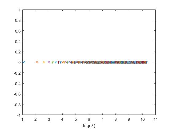
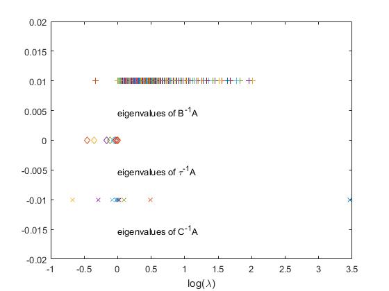
Figure 1: The spectral distribution of coefficient matrix $A$ and preconditioned matrices $P^{-1}A$.

Table 2: Extreme eigenvalues of preconditioned matrix ${\tau}^{-1}A$ of Example 6.1 with $\alpha=1.8$.

n	$2^{6}$	$2^{7}$	$2^{8}$	$2^{9}$	$2^{10}$	$2^{11}$	$2^{12}$
$\lambda_{\max}$	1.0001	1.0001	1.0001	1.0001	1.0001	1.0001	1.0001
$\lambda_{\min}$	0.8721	0.8586	0.8473	0.8379	0.8300	0.8232	0.8173

Example 6.2.

In this example, we consider $2D$ Riesz fractional diffusion equations in ${\Omega}\in[0,1]\times[0,1]$, where the exact solution is

$$u(x_{1},x_{2})=x_{1}^{2}(1-x_{1})^{2}{x_{2}}^{2}(1-x_{2})^{2}.$$

Take the diffusion coefficients $d_{1}=d_{2}=1$. The source term is given by

$$y= \frac{d_{1}}{\cos(\pi\alpha_{1}/2)}x_{2}^{2}(1-x_{2})^{2}(y_{1}(x_{1},\alpha_{1})+y_{1}(1-x_{1},\alpha_{1}))$$

$$+\frac{d_{2}}{\cos(\pi\alpha_{2}/2)}x_{1}^{2}(1-x_{1})^{2}(y_{1}(x_{2},\alpha_{2})+y_{1}(1-x_{2},\alpha_{2})),$$

where

$$y_{1}(x,\alpha)=\frac{2}{\Gamma(3-\alpha)}x^{2-\alpha}-\frac{12}{\Gamma(4-\alpha)}x^{3-\alpha}+\frac{24}{\Gamma(5-\alpha)}x^{4-\alpha}.$$

Table 3: Comparisons for solving Example 6.2 for different ${\alpha}$ by the CG method, and the PCG methods with the ${\tau}$-preconditioner, and the circulant preconditioner, and multigrid methods.

$(\alpha_{1},\alpha_{2})$	$n_{1}+1$	${\tau}_{pre}$		$C_{pre}$		$M_{pre}$		$MGM$		$N_{pre}$
		Iter	CPU(s)	Iter	CPU(s)	Iter	CPU(s)	Iter	CPU(s)	Iter	CPU(s)
(1.1,1.2)	$2^{6}$	7	0.11	17	0.39	13	0.64	13	0.09	93	0.75
	$2^{7}$	7	0.21	19	0.45	14	0.89	11	0.45	157	3.63
	$2^{8}$	8	1.37	21	2.17	17	4.42	10	2.89	237	12.34
	$2^{9}$	8	5.06	24	9.84	22	12.20	9	5.59	383	82.59
	$2^{10}$	9	13.03	27	29.56	31	80.05	9	24.33	585	490.56
(1.4,1.5)	$2^{6}$	7	0.22	16	0.33	12	0.72	12	0.50	91	0.78
	$2^{7}$	7	0.31	19	0.45	13	0.86	11	0.80	157	3.25
	$2^{8}$	8	1.08	23	2.08	16	3.78	12	3.14	269	14.23
	$2^{9}$	8	4.34	28	11.78	23	13.27	12	7.56	457	90.08
	$2^{10}$	9	12.56	32	34.11	36	96.06	13	31.25	771	615.25
(1.8,1.9)	$2^{6}$	6	0.10	19	0.53	11	0.59	16	0.11	126	0.86
	$2^{7}$	6	0.14	24	1.05	12	0.75	15	0.72	243	5.28
	$2^{8}$	7	0.67	31	2.84	12	4.28	15	3.77	467	27.97
	$2^{9}$	7	2.92	40	15.91	22	12.45	16	9.64	901	178.20
	$2^{10}$	7	10.42	52	54.52	34	85.94	17	40.53	1740	1383.60
(1.2,1.8)	$2^{6}$	6	0.17	19	0.27	9	0.58	42	0.39	127	1.05
	$2^{7}$	7	0.31	27	0.83	10	0.73	60	2.50	247	5.06
	$2^{8}$	7	1.22	33	3.20	14	3.94	87	19.28	463	24.30
	$2^{9}$	8	4.05	44	18.80	21	12.44	126	73.89	881	173.53
	$2^{10}$	8	11.56	58	61.42	30	73.19	184	402.94	1671	1352.76

In the 2D case, we exploit the multigrid preconditioned method and the algebraic multigrid method for comparisons, where the weight of the Jacobi iterative method is chosen as $w=2/3$.

In this example, we take $n_{1}=n_{2}$. From Table 3, note that both of the number of iterations and the CPU time provided by the $\tau$-preconditioner are much less than those by other methods. It demonstrates the superiority of the $\tau$-preconditioner.

Example 6.3.

In this example, we test 3D Riesz fractional diffusion equations. Consider

$${\Omega}=[0,1]\times[0,1]\times[0,1],\ d_{1}=d_{2}=d_{3}=1,$$

$$y= \frac{d_{1}}{\cos(\pi\alpha_{1}/2)}x_{2}^{2}(1-x_{2})^{2}x_{3}^{2}(1-x_{3})^{2}(y_{1}(x_{1},\alpha_{1})+y_{1}(1-x_{1},\alpha_{1}))$$

$$+\frac{d_{2}}{\cos(\pi\alpha_{2}/2)}x_{1}^{2}(1-x_{1})^{2}x_{3}^{2}(1-x_{3})^{2}(y_{1}(x_{2},\alpha_{2})+y_{1}(1-x_{2},\alpha_{2}))$$

$$+\frac{d_{3}}{\cos(\pi\alpha_{3}/2)}x_{1}^{2}(1-x_{1})^{2}x_{2}^{2}(1-x_{2})^{2}(y_{1}(x_{3},\alpha_{3})+y_{1}(1-x_{3},\alpha_{3})).$$

The exact solution is $u=x_{1}^{2}(1-x_{1})^{2}{x_{2}}^{2}(1-x_{2})^{2}{x_{3}}^{2}(1-x_{3})^{2}$.

Table 4: Comparisons for solving Example 6.3 for different ${\alpha}$ by the CG method, and the PCG methods with the ${\tau}$-preconditioner and the circulant preconditioner.

$(\alpha_{1},\alpha_{2},\alpha_{3})$	$n_{1}+1$	${\tau}_{pre}$		$C_{pre}$		$N_{pre}$
		Iter	CPU(s)	Iter	CPU(s)	Iter	CPU(s)
(1.1,1.2,1.3)	$2^{4}$	6	0.19	14	0.31	40	0.28
	$2^{5}$	6	0.73	17	1.41	70	3.67
	$2^{6}$	7	5.34	21	11.88	118	36.27
	$2^{7}$	8	29.39	24	69.69	191	288.64
	$2^{8}$	8	226.28	27	521.38	304	2.98e+3
(1.4,1.5,1.6)	$2^{4}$	6	0.22	15	0.40	39	0.19
	$2^{5}$	7	0.48	18	1.42	71	3.69
	$2^{6}$	7	4.77	22	11.03	128	36.64
	$2^{7}$	7	25.84	25	72.28	223	335.20
	$2^{8}$	8	200.64	32	611.23	387	3.77e+3
(1.7,1.8,1.9)	$2^{4}$	5	0.23	16	0.45	45	0.25
	$2^{5}$	6	0.64	20	1.59	88	4.06
	$2^{6}$	6	3.93	26	13.88	169	50.38
	$2^{7}$	6	24.34	35	95.42	328	495.33
	$2^{8}$	7	180.61	44	832.36	628	6.08e+3
(1.2,1.5,1.8)	$2^{4}$	6	0.25	16	0.36	43	0.23
	$2^{5}$	6	0.64	20	1.63	83	3.73
	$2^{6}$	7	4.95	25	13.70	157	48.13
	$2^{7}$	8	18.11	33	94.09	295	441.98
	$2^{8}$	8	198.59	44	828.98	551	5.34e+3

In this example, let $n_{1}=n_{2}=n_{3}$. It is evident that the ${\tau}$-preconditioner is still efficient for 3D Riesz fractional diffusion equations from the Table 4. In contrast with the circulant preconditioner, the number of iterations by the ${\tau}$-preconditioner is almost unchanged when the matrix size increases. Hence, ${\tau}$-preconditioner is an excellent tool for solving ill-conditioned multi-level Toeplitz systems arising from multi-dimensional Riesz fractional diffusion equations.

Finally, we verify the effectiveness of the preconditioning of discretized Riesz fractional derivatives for handling the ill-conditioned multi-level Toeplitz matrices whose generating functions are with fractional order zeros at the origin.

Example 6.4.

Consider a two-level Toeplitz matrix whose generating function is defined by

$$p_{{\boldsymbol{\alpha}}}({\boldsymbol{\theta}})=p_{\alpha_{1}}(\theta_{1})+p_{\alpha_{2}}(\theta_{2})-p_{1}(\theta_{1})p_{1}(\theta_{2}),$$

where (see [8])

$$p_{\alpha_{i}}({\theta_{i}})=\left\{\begin{array}[]{cc}|{\theta_{i}}|^{\alpha_{i}},&|{\theta_{i}}|<\frac{\pi}{2},\\ 1,&|{\theta_{i}}|\geq\frac{\pi}{2}.\end{array}\right.$$

It is obvious that

$$0<\frac{4-\pi}{4}\leq\frac{p_{{\boldsymbol{\alpha}}}({\boldsymbol{\theta}})}{q_{{\boldsymbol{\alpha}}}({\boldsymbol{\theta}})}\leq 1,$$

where $q_{{\boldsymbol{\alpha}}}({\boldsymbol{\theta}})$ is defined in (5.3) with $l_{1}=l_{2}=1$. The above inequality exemplifies that the generating function $p_{{\boldsymbol{\alpha}}}({\boldsymbol{\theta}})$ satisfies the 1.

Table 5: Comparisons for solving Example 6.4 for different ${\alpha}$ by the CG method, and the PCG methods with the ${\tau}$-preconditioner, the circulant preconditioner, and our preconditioner, and the algebraic multigrid method.

$(\alpha_{1},\alpha_{2})$	$n_{1}+1$	$R_{pre}$		${\tau}_{pre}$		$C_{pre}$		$N_{pre}$		$MGM$
		Iter	CPU(s)	Iter	CPU(s)	Iter	CPU(s)	Iter	CPU(s)	Iter	CPU(s)
(1.9,1.5)	$2^{6}$	26	0.42	13	0.23	26	0.31	79	0.36	9	0.22
	$2^{7}$	26	0.92	13	0.44	36	1.17	134	2.95	10	0.67
	$2^{8}$	27	4.97	16	2.58	45	4.81	225	15.69	12	2.36
	$2^{9}$	27	15.41	19	12.77	69	35.14	376	136.80	14	11.75
	$2^{10}$	27	46.48	25	50.16	192	278.50	566	572.09	18	58.38
	$2^{11}$	27	188.77	42	302.30	239	1.44e+3	956	4.19e+3	21	329.05
	$2^{12}$	27	659.05	57	1.36e+3	782	–	*	–	26	1.71e+3
(1.9,1.7)	$2^{6}$	26	0.53	14	0.14	29	0.63	90	0.42	9	0.22
	$2^{7}$	26	0.84	17	0.63	44	1.34	159	4.44	9	0.77
	$2^{8}$	26	3.95	20	2.98	79	8.02	278	20.34	10	2.24
	$2^{9}$	26	15.47	30	19.05	145	73.41	467	132.67	11	9.77
	$2^{10}$	27	47.89	49	83.78	270	385.14	846	907.67	12	48.60
	$2^{11}$	27	188.72	85	565.31	736	5.20e+3	*	–	13	216.62
	$2^{12}$	27	690.84	219	5.09e+3	*	–	*	–	15	1.01e+3
(1.9,1.9)	$2^{6}$	27	0.39	15	0.19	30	0.27	97	0.64	9	0.33
	$2^{7}$	27	0.91	21	0.93	57	1.77	179	3.56	9	0.64
	$2^{8}$	27	4.17	26	4.12	85	8.58	327	22.75	9	2.33
	$2^{9}$	27	17.27	44	26.34	212	111.33	573	210.27	9	8.41
	$2^{10}$	27	47.45	80	135.02	622	884.95	943	948.84	9	37.30
	$2^{11}$	27	190.06	195	1.29e+3	*	–	*	–	10	166.47
	$2^{12}$	27	660.47	530	–	*	–	*	–	10	683.06

To test the efficiency of our proposed preconditioner defined in (33), the PCG methods with the ${\tau}$-preconditioner, the circulant preconditioner, and the case without preconditioner are proposed as comparisons. Denote our preconditioner as ‘$R_{pre}$’ in Table 5.

From Table 5, we see that the number of iterations deriving from the circulant preconditioner, the natural ${\tau}$-preconditioner, and no preconditioner increase rapidly as the matrices size increase, while that by our proposed preconditioner almost keeps constant. In terms of the multigrid method, we observe that the method implements well when the orders of the zeros are closed. Since the cost per iteration of using the algebraic multigrid method is about $8/3$ times than the required by the $\tau$-preconditioner [35], in light of Table 5, we derive that the performance of the multigrid method is as efficient as the proposed method. Nevertheless, the multigrid method will be inefficient provided that the orders of the zeros are quite difference; see the item for $(\alpha_{1},\alpha_{2})=(1.9,1.5)$ in Table 5. Moreover, the linearly convergent rate is still a question for these cases by the algebraic multigrid method.

7 Conclusion remarks

In this paper, we have studied the spectra of the $\tau$-preconditioned matrices for the multi-level Toeplitz systems arising from the multi-dimensional Riesz spatial fractional diffusion equations. Theoretically, we have proved that the spectra of the preconditioned matrices are bounded below by 1/2 and bounded above by 3/2, and hence the condition numbers of the preconditioned matrices are all less than $3$. Besides, we proposed a new preconditioner for ill-conditioned multi-level Toeplitz systems, which are generated by the generating functions with fractional order zeros at the origin. We have proved that the spectra of the proposed preconditioned matrices are bounded by constants which are independent of the matrices size. The numerical results have revealed that the performance of the proposed preconditioner is much better than that of other existing methods. In our future work, we will consider to combine the ${\tau}$-preconditioner with other methods to handle more general (non-symmetric) multi-level Toeplitz-like systems arising from multi-dimensional fractional partial differential equations.

References

• [1] N. Barakitis, S. E. Ekström and P. Vassalos, Preconditioners for fractional diffusion equations based on the spectral symbol, ArXiv preprint arXiv: 1912.13304 (2019).
• [2] F. Di Benedetto, Preconditioning of block Toeplitz matrices by sine transforms, SIAM J. Sci. Comput., 18 (1997), pp. 499–515.
• [3] F. Di Benedetto, G. Fiorentino and S. Serra Capizzano, CG preconditioning for Toeplitz matrices, Comput. Math. Appl., 25 (1993), pp. 35–45.
• [4] D. Bini and F. Benedetto, A new preconditioner for the parallel solution of positive definite Toeplitz systems, in Proceedings, 2nd SPAA Conference, Crete, Greece, July 1990, pp. 220–223.
• [5] D. Bini and M. Capovani, Spectral and computational properties of band symmetric Toeplitz matrices, Linear Algebra Appl., 52/53 (1983), pp. 99–126.
• [6] A. Böttcher and S. Grudsky, On the condition numbers of large semi-definite Toeplitz matrices, Linear Algebra Appl., 279 (1998), pp. 285–301.
• [7] R. H. Chan, Toeplitz preconditioner for Toeplitz system with nonnegative generating function, IMA J. Numer. Anal., 11 (1991), pp. 333–345.
• [8] R. H. Chan, Q. S. Chang and H. W. Sun, Multigrid method for ill-conditioned symmetric Toeplitz systems, SIAM J. Sci. Comput., 19 (1998), pp. 516–529.
• [9] R. H. Chan, M. K. Ng and C. K. Wong, Sine transform based preconditioners for symmetric Toeplitz systems, Linear Algebra Appl., 232 (1996), pp. 237–259.
• [10] R. H. Chan, A. M. Yip and M. K. Ng, The best circulant preconditioners for Hermitian Toeplitz systems, SIAM J. Numer. Anal., 38 (2000), pp. 876–896.
• [11] W. K. Ching, Iterative methods for Queuing and Manufacturing systems, Springer-Verlag, London, 2001.
• [12] H. F. Ding and Y. X. Zhang, New numerical methods for the Riesz space fractional partial differential equations, Comput. Math. Appl., 63 (2012), pp. 1135–1146.
• [13] M. Donatelli, R. Krause, M. Mazza and K. Trotti, Multigrid preconditioners for anisotropic space-fractional diffusion equations, Adv Comput Math., 49 (2020).
• [14] M. Donatelli, M. Mazza and S. Serra Capizzano, Spectral analysis and structure preserving preconditioners for fractional diffusion equations, J. Comput. Phys., 307 (2016), pp. 262–279.
• [15] G. Fiorentino and S. Serra Capizzano, Multigrid methods for Toeplitz matrices, Calcolo., 28 (1991), pp. 283–305.
• [16] G. Fiorentino and S. Serra Capizzano, Multigrid methods for symmetric positive definite block Toeplitz matrices with nonnegative generating functions, SIAM J. Sci. Comput., 17 (1996), pp. 1068–1081.
• [17] U. Grenander and G. Szegö, Toeplitz Forms and Their Applications, 2nd ed., Chelsea, New York, 1984.
• [18] R. Hilfer, Applications of Fractional Calculus in Physics, World Scientific, Singapore, 2000.
• [19] R. A. Horn and C. R. Johnson, Matrix Analysis, Cambridge University Press, Cambridge, 2012.
• [20] S. L. Lei and H. W. Sun, A circulant preconditioner for fractional diffusion equations, J. Comput. Phys., 242 (2013, pp. 715–725.
• [21] F. R. Lin, S. W. Yang and X. Q. Jin, Preconditioned iterative methods for fractional diffusion equation, J. Comput. Phys., 256 (2014), pp. 109–117.
• [22] M. M. Meerschaert and C. Tadjeran, Finite difference approximations for fractional advection-dispersion flows equations, J. Comput. Appl. Math., 172 (2004), pp. 209–219.
• [23] H. Moghaderi, M. Dehghan, M. Donatelli and M. Mazza, spectral analysis and multigrid preconditioners for two-dimensional space-fractional diffusion equations, J. Comput. Phys., 350 (2017), pp. 992–1011.
• [24] D. Noutsos, S. Serra Capizzano and P. Vassalos, Matrix algebra preconditioners for multilevel Toeplitz systems do not insure optimal convergence rate, Theor Comput Sci., 315 (2004), pp. 557–579.
• [25] D. Noutsos, S. Serra Capizzano and P. Vassalos, Essential spectral equivalence via multiple step preconditioning and applications to ill conditioned Toeplitz matrices, Linear Algebra Appl., 491 (2016), pp. 276–291.
• [26] H. K. Pang and H. W. Sun, Fast numerical contour integral method for fractional diffusion equations, J. Sci. Comput., 66 (2016), pp. 41–66.
• [27] J. Pestana, Preconditioners for symmetrized Toeplitz and multi-level Toeplitz matrices, SIAM J. Matrix. Anal. Appl., 44 (2019), pp. 870–887.
• [28] I. Podlubny, Fractional differential equations, Academic Press, New York, 1999.
• [29] D. Potts and G. Steidl, Preconditioners for ill-conditioned Toeplitz Matrices, BIT., 39 (1999), pp. 513–533.
• [30] D. Potts and G. Steidl, Preconditioners for ill-conditioned Toeplitz systems constructed from positive kernels, SIAM J. Sci. Comput., 22 (2001), pp. 1741–1761.
• [31] A. I. Saichev and G. M. Zaslavsky, Fractional kinetic equations: solutions and applications, Chaos., 7 (1997), pp. 753–764.
• [32] S. Serra Capizzano, New PCG based algorithms for the solution of Hermitian Toeplitz systems, Calcolo., 32 (1995), pp. 153–176.
• [33] S. Serra Capizzano, On the extreme eigenvalues of Hermitian (block) Toeplitz matrices, Linear Algebra Appl., 270 (1998), pp. 109–129.
• [34] S. Serra Capizzano, Superlinear PCG methods for symmetric Toeplitz systems, Math. Comput., 68 (1999), pp. 793–803.
• [35] H. W. Sun, X. Q. Jin and Q. S. Chang, Convergence of the multigrid method for ill-conditioned block Toeplitz systems, BIT., 41 (2001), pp. 179–190.
• [36] V. E. Tarasov, Fractional Dynamics: Applications of Fractional Calculus to Dynamics of Particles, Fields and Media Higher Education Press, Beijing, 2010.