On weakly and strongly popular rankings

Abstract

Van Zuylen et al. [35] introduced the notion of a popular ranking in a voting context, where each voter submits a strict ranking of all candidates. A popular ranking $\pi$ of the candidates is at least as good as any other ranking $\sigma$ in the following sense: if we compare $\pi$ to $\sigma$, at least half of all voters will always weakly prefer $\pi$. Whether a voter prefers one ranking to another is calculated based on the Kendall distance.

A more traditional definition of popularity—as applied to popular matchings, a well-established topic in computational social choice—is stricter, because it requires at least half of the voters who are not indifferent between $\pi$ and $\sigma$ to prefer $\pi$. In this paper, we derive structural and algorithmic results in both settings, also improving upon the results in [35]. We also point out connections to the famous open problem of finding a Kemeny consensus with three voters.

additions

1 Introduction

A fundamental question in preference aggregation is the following: given a number of voters who rank candidates from most-preferred to least-preferred, can we construct a ranking that expresses the preferences of the entire set of voters as a whole? A common way of evaluating how close the constructed ranking is to a voter’s preferences is the Kendall distance [28], which measures the pairwise disagreements between two rankings. Among others, a well-known rank aggregation method is the Kemeny ranking method [27], in which the winning ranking minimises the sum of its Kendall distances to the voters’ rankings.

For the preference aggregation problem, van Zuylen et al. [35] introduce a new rank aggregation method called popular ranking, which is also based on the Kendall distance. Each voter can compare two given rankings $\pi$ and $\sigma$, and prefers the one that is closer to her submitted ranking in terms of the Kendall distance. Van Zuylen et al. define $\pi$ to be a winning ranking for a given set of voters’ rankings if for any ranking $\sigma$, at least half of the voters prefer $\pi$ to $\sigma$ or are indifferent between them. This implies that there is no ranking $\sigma$ such that switching to $\sigma$ from $\pi$ would benefit a majority of all voters.

According to the definition of popularity in [35], even in a situation where exactly half of the voters are indifferent between rankings $\pi$ and $\sigma$—we call these abstaining voters—, whilst the other half of the voters prefer $\sigma$ to $\pi$, the ranking $\sigma$ is not more popular than $\pi$. This example demonstrates how challenging it is for the dissatisfied voters to propose a ranking that overrules $\pi$—the definition requires them to find a profiting set of voters who build an absolute majority, that is, a majority of all voters for this endeavour.

A straightforward option would be to require only a simple majority, this is, a majority of the non-abstaining voters, to profit from switching to $\sigma$ from $\pi$. Excluding the abstaining voters in a pairwise majority voting rule is common practice [15]. It is also analogous to the classical popularity notion in the matching literature [1]. In this paper, we propose an alternative definition of a popular ranking. We define $\pi$ to be a strongly popular ranking if for every ranking $\sigma$, at least half of the non-abstaining voters prefer $\pi$ to $\sigma$. This means that switching from $\pi$ to $\sigma$ would harm at least as many voters as it would benefit. The weaker notion of a popular ranking as defined by van Zuylen et al. [35] is then defined here as a weakly popular ranking.

1.1 Our contribution

We study both the weaker notion of popularity from [35] and the stronger notion of popularity analogous to the one in the matching literature, which excludes abstaining voters. Our most important results are as follows.

1. We give a sufficient condition for the existence of a weakly popular ranking (Theorem 4.1).

2. We give a sufficient condition for the two popularity notions to be equivalent for a given ranking $\pi$ (Lemma 3.7). This condition also implies that at least three abstaining voters between two rankings are needed for the two popularity notions to differ, which allows us to deduce the following result.

3. For at most five voters, the two popularity notions are equivalent (Theorem 3.14). We provide an example showing that with six voters this equivalence does not hold anymore (Theorem 3.4).

4. In the case of two or three voters, one can find a popular ranking of either kind and verify the weak or strong popularity of a given ranking in polynomial time (Lemmas 4.5 and 4.6, Theorem 4.7).

5. The problem of verifying the weak or strong popularity of a given ranking is polynomial-time solvable for four voters if and only if it is polynomial-time solvable for five voters (Theorem 4.18).

6. Finally, we establish a connection to a central open problem in preference aggregation. We show that if finding a ranking that is more popular in either sense than a given ranking in a given set of four (or five) voters’ rankings were polynomial-time solvable, then the famously open Kemeny consensus problem for three voters would also be polynomial-time solvable (Corollary 5.5). The path to this result leads through an even stronger observation: If finding a ranking preferred to a given ranking by all the three voters were polynomial-time solvable, then the Kemeny consensus problem for three voters would also be polynomial-time solvable (Theorems 5.2 and 5.1).

1.2 Related literature

Aggregating voters’ preferences given as rankings of candidates has been challenging researchers for decades. The most common approach to this problem is to search for a ranking that minimises the sum of the distances to the voters’ rankings. If the Kendall distance [28] is used as the metric on rankings, then this optimality concept corresponds to the Kemeny consensus [27]. Characteristic properties and computational aspects of the Kemeny consensus have been studied in a number of papers [6, 14, 23, 7, 2]. The problem setting with a small number of voters received special interest. Deciding whether a given ranking is a Kemeny consensus is $\coNP$-complete [18], and calculating a Kemeny consensus is $\NP$-hard [6] even if there is a fixed number of voters $k$, where $k=7$ [3], or where $k$ is even and $k\geq 4$ [16]. The complexity of the problem for three and five voters is pointed out as an interesting open problem in [8, 3]. Milosz et al. [32] focus on the case of three voters, and establish a link with the 3-Hitting Set problem [25] by considering 3-cycles in the majority graph.

Majority voting rules offer another natural way of aggregating voters’ preferences. The earliest reference for this might be from Condorcet [10], who uses pairwise comparisons to calculate the winning candidate, establishing his famous paradox on the smallest set of voters’ rankings not admitting any majority winner.

In some settings, handling abstaining voters plays a crucial role. The absolute and simple majority voting rules have both been extensively discussed in the setting where the goal is to choose the winning candidate [4, 5]. Vermeule [36] focuses on strategic minorities and demonstrates the effect of the simple majority rule compared to the absolute majority rule based on data from decisions made by the United States Congress. By undertaking a probabilistic analysis, Dougherty and Edward [15] discuss the differences between the two rules. Felsenthal and Machover [30] generalise simple voting games to ternary voting games by adding the possibility to abstain.

The concept of majority voting readily translates to other scenarios, where voters submit preference lists. One such field is the area of matchings under preferences, where popular matchings 21, 1, 31, Chapter 7, 11 serve as a voting-based alternative concept to the well-known notion of stable matchings [20] in two-sided markets. In short, a popular matching $M$ is a simple majority winner among all matchings, because it guarantees that no matter what alternative matching is offered on the market, at least half of the non-abstaining voters will opt for $M$.

Besides two-sided matchings, majority voting has also been defined for the house allocation problem [1, 33], the roommates problem [17, 22], spanning trees [12], permutations [35], the ordinal group activity selection problem [13], and very recently, for branchings [26]. The notion of popularity is aligned with simple majority in all these papers, with one exception, namely [35], which defines popularity based on the absolute majority rule.

A part of this work revisits the paper from van Zuylen et al. [35]. They show that a popular ranking—according to their definition of popularity—need not necessarily exist. More precisely, they show that the acyclicity of a structure known as the majority graph is a necessary, but not sufficient condition for the existence of a popular ranking. They also prove that if the majority graph is acyclic, then we can efficiently compute a ranking (corresponding to a toplogical sort of the majority graph), which may or may not be popular, but for which the voters have to solve an $\NP$-hard problem to compute a ranking that a majority of them prefer.

1.3 Structure of the paper

In Section 2 we introduce the necessary definitions and notations used in the following sections. Section 3 deals with the relationship between the two different popularity notions. In Section 4 we study the complexity of the problems of deciding whether a given ranking is weakly or strongly popular with a small number of voters. We demonstrate the strong connection to the Kemeny consensus problem in Section 5. Finally, we lay out some problems that still remain to be answered in Section 6. Throughout this paper, we use the example instance depicted in Figure 1 to illustrate concepts that we will define.

2 Preliminaries

We start this section with the formal definitions of various standard notions in voting theory in Section 2.1. Then, in Section 2.2, we introduce weakly and strongly popular rankings and the decision problems we will later analyse.

2.1 Rankings and Kendall distance

We are given a set $C=\{1,\ldots,m\}$ of candidates and a set $V=\{v_{1},\ldots,v_{n}\}$ of $n$ voters. A (preference) ranking $\pi$ is a total order over $C$. When exhibiting a specific ranking, we will often enclose parts of it in square brackets, e.g. we may write $[1,2],[3,4]$ instead of $1,2,3,4$. These brackets can be ignored and are simply used for better readability in sets of rankings with specific structural properties. The rank of candidate $a$ in ranking $\pi$ is the position (counting from 1) it appears at in $\pi$, and it is denoted by $\operatorname{rank}_{\pi}[a]$. A profile $P=(\pi_{v_{1}},\ldots,\pi_{v_{n}})$ over $C$ is a list of rankings, where $\pi_{v_{i}}$ is the ranking associated with voter $v_{i}\in V$. An example is depicted in Figure 1. We say that voter $v$ prefers candidate $a$ to candidate $b$ if $\operatorname{rank}_{\pi_{v}}[a]<\operatorname{rank}_{\pi_{v}}[b]$. In Figure 1, voter $v_{1}$ prefers candidate $1$ to candidate $2$, and $\operatorname{rank}_{\pi_{v_{1}}}[5]=6$. For candidates $a$ and $b$, $\{a,b\}$ denotes the unordered pair of them, while $(a,b)$ denotes an ordered pair.

$$\pi_{v_{1}} =[1,2,3],[6,4,5],[8,9,7]$$

$$\pi_{v_{2}} =[2,3,1],[4,5,6],[9,7,8]$$

$$\pi_{v_{3}} =[3,1,2],[5,6,4],[7,8,9]$$

$$\pi_{v_{4}} =[1,2,3],[4,5,6],[7,8,9]$$

$$\pi_{v_{5}} =[1,2,3],[5,4,6],[9,7,8]$$

$$\pi_{v_{6}} =[1,2,3],[5,6,4],[7,9,8]$$

Figure 1: A profile $P=(\pi_{v_{1}}\ldots,\pi_{v_{6}})$ over $\{1,2,\ldots,9\}$.

We say that voter $v_{1}$ (or ranking $\pi_{v_{1}}$) agrees with voter $v_{2}$ (or with ranking $\pi_{v_{2}}$) in the order of two distinct candidates $a$ and $b$ if $v_{1}$ and $v_{2}$ either both prefer $a$ to $b$ or they both prefer $b$ to $a$. Otherwise they disagree in the order of $a$ and $b$. The similarity between two rankings can be measured by various metrics defined on permutations. Possibly the most common metric, the Kendall distance [28], is defined below.

Definition 2.1.

The Kendall distance $K(\pi,\sigma)$ between two rankings $\pi$ and $\sigma$ is defined as the number of pairwise disagreements between $\pi$ and $\sigma$, or, formally as

$$K(\pi,\sigma)={\color[rgb]{0,0,0}|\{(a,b){\color[rgb]{0,0,0}\in C\times C}:\operatorname{rank}_{\pi}[a]>\operatorname{rank}_{\pi}[b]\mbox{ and }\operatorname{rank}_{\sigma}[a]<\operatorname{rank}_{\sigma}[b]\}|.}$$

Alongside Definition 2.1, the Kendall distance has an interpretation, which we will also use, in terms of the bubble sort algorithm [19]. Given a sequence $\langle\sigma_{1},\sigma_{2},\dots,\sigma_{m}\rangle$, bubble sort proceeds inductively by considering the $i$th element $\sigma_{i}$ ($i=1,2,\dots,m$), and assuming that $\langle\sigma_{1},\sigma_{2},\dots\sigma_{i-1}\rangle$ are already in the correct order, $\sigma_{i}$ is swapped with its predecessor in $\langle\sigma_{1},\sigma_{2},\dots,\sigma_{i-1},\sigma_{i}\rangle$ as long as $\sigma_{i}$ is larger than its predecessor in this subsequence. The Kendall distance is also called the bubble sort distance because it corresponds to the number of swaps that bubble sort executes when converting ranking $\pi$ to ranking $\sigma$. To be more precise, let us first define a total order on $1,\ldots,n$ such that, under this order, ranking $\sigma$ is sorted in increasing order. We define the bubble swap path from a ranking $\pi$ to $\sigma$ as the sequence $\pi_{0}:=\pi,\pi_{1},\ldots,\pi_{k}:=\sigma$ of intermediate rankings obtained when sorting $\pi$ using the bubble sort algorithm. Note that $K(\pi,\sigma)=k$. We call the change $\pi_{i}\rightarrow\pi_{i+1}$ a swap. Alternatively we denote the swap by the consecutive candidates $a$ and $b$ it interchanges: $(b,a)\rightarrow(a,b)$. We say that a swap $(b,a)\rightarrow(a,b)$ is good for voter $v$ if $v$ prefers $a$ to $b$, otherwise this swap is bad for $v$. Note that if the swap $\pi_{i}\rightarrow\pi_{i+1}$ is good for $v$, then $K(\pi_{i+1},\pi_{v})=K(\pi_{i},\pi_{v})-1$ and, analogously, if the swap is bad for $v$, then $K(\pi_{i+1},\pi_{v})=K(\pi_{i},\pi_{v})+1$.

For example, with respect to the profile shown in Figure 1, $K(\pi_{v_{1}},\pi_{v_{2}})=6$, since it takes two swaps to insert each of $1$, $6$ and $8$ into the correct order relative to $[2,3,1]$, $[4,5,6]$ and $[9,7,8]$, respectively, in the bubble swap path from $\pi_{v_{1}}$ to $\pi_{v_{2}}$.

Let $V(a,b)\subseteq V$ be the set of voters who prefer candidate $a$ to $b$, i.e. $V(a,b)=\{v\in V:\operatorname{rank}_{\pi_{v}}(a)<\operatorname{rank}_{\pi_{v}}(b)\}$. The majority graph belonging to a profile is defined as the directed graph which has as vertices the candidates and an arc from candidate $a$ to candidate $b$ if a majority of the voters prefer $a$ to $b$, i.e. $|V(a,b)|>|V(b,a)|$. As mentioned in the introduction, Condorcet observed that the majority graph may contain a directed cycle. This has come to be known as the Condorcet paradox [10]. A tournament is a majority graph that is complete, or, in other words, for every $a$ and $b$ either $|V(a,b)|>|V(b,a)|$ or $|V(a,b)|<|V(b,a)|$ holds. The majority graph of our profile in Figure 1 is depicted in Figure 2. As the edges form no cycle, it is an acyclic majority graph, but since it is not a complete graph, it is not a tournament.

Figure 2: The majority graph of the profile from Figure 1. Each grey set of three candidates denotes a specific subgraph that satisfies the same property as a component in a tournament [29]. Arcs between these components symbolise the complete set of 9 arcs, between any two vertices from different components.

Ranking $\pi$ is a topologically sorted ranking of profile $P$ if $\operatorname{rank}_{\pi}[a]<\operatorname{rank}_{\pi}[b]$ holds for each pair of candidates $a$ and $b$ with $|V(a,b)|>|V(b,a)|$. Topologically sorted rankings correspond to the graph-theoretical topological sort of the vertices in the majority graph, and thus only exist if the majority graph is acyclic. Acyclic tournaments trivially have a unique topologically sorted ranking. A topologically sorted ranking for the profile in Figure 1 with $9$ candidates is $\sigma=[1,2,3],[4,5,6],[7,8,9]$, as can be checked easily.

The Kemeny rank of a ranking $\pi$ for a given profile with voters $v_{1},\ldots,v_{n}$ is defined as $\sum_{i=1}^{n}K(\pi,\pi_{v_{i}})$. If ranking $\sigma$ has minimum Kemeny rank over all rankings, then $\sigma$ is a Kemeny consensus [27]. The following well-known observation [14] will be useful in our proofs.

Observation 2.2.

Each topologically sorted ranking is a Kemeny consensus. For acyclic majority graphs, the set of topologically sorted rankings coincides with the set of Kemeny consensuses.

2.2 Popularity and problem definitions

Preferences over rankings

Voters prefer rankings that are similar to their submitted ranking. More precisely, voter $v$ prefers ranking $\sigma$ to ranking $\pi$ if $K(\sigma,\pi_{v})<K(\pi,\pi_{v})$. Analogously, voter $v$ abstains between $\pi$ and $\sigma$ if $K(\sigma,\pi_{v})=K(\pi,\pi_{v})$. We will simply call $v$ an abstaining voter if $\pi$ and $\sigma$ are clear from the context.

For example, let $\sigma_{1}=[1,2,3],[5,6,4],[9,7,8]$ and $\sigma_{2}=[1,2,3],\allowbreak[4,5,6],[7,8,9]$. Looking back at Figure 1, clearly $v_{4}$ prefers $\sigma_{2}$ to $\sigma_{1}$, since $\pi_{v_{4}}=\sigma_{2}$ and $\pi_{v_{4}}\neq\sigma_{1}$, that is, $K(\pi_{v_{4}},\sigma_{2})=0<K(\pi_{v_{4}},\sigma_{1})$. Voter $v_{1}$ in the same profile is an abstaining voter since $K(\pi_{v_{1}},\sigma_{2})=4=K(\pi_{v_{1}},\sigma_{1})$. For more detail regarding these calculations, the reader is referred to A.

Majority concepts

We now formally define the two majority concepts we rely on in this paper. A set $V^{\prime}\subseteq V$ of voters forms an absolute majority of the voters if $|V^{\prime}|>n/2$. For the more intricate majority concept, two rankings $\pi$ and $\sigma$ must be given. Let $V_{\text{abs}}(\pi,\sigma)$ be the set of voters who abstain in the vote between rankings $\pi$ and $\sigma$, that is, $v\in V_{\text{abs}}(\pi,\sigma)$ if and only if $K(\pi_{v},\pi)=K(\pi_{v},\sigma)$. In Figure 1, $V_{\text{abs}}(\sigma_{1},\sigma_{2})=\{v_{1},v_{2},v_{3}\}$, where $\sigma_{1}$ and $\sigma_{2}$ are as defined in the previous paragraph. A set $V^{\prime}\subseteq V$ of voters forms a simple majority of the voters if $|V^{\prime}|>|V\setminus V_{\text{abs}}(\pi,\sigma)|/2$. A simple majority therefore always depends on the rankings that are being compared.

Popularity concepts

We now define the two different notions of popularity. The first notion of a weakly popular ranking corresponds to the popular ranking as defined in [35]. Let $C$ be a set of candidates and let $P$ be a profile over $C$ of voters $V$.

Definition 2.3.

Ranking $\pi^{\prime}$ is more popular than ranking $\pi$ in the absolute sense if $K(\pi^{\prime},\pi_{v})<K(\pi,\pi_{v})$ for an absolute majority of all voters $v\in V$. Ranking $\pi$ is weakly popular for $P$ if no ranking $\pi^{\prime}$ is more popular than $\pi$ in the absolute sense, in other words, if there is no ranking $\pi^{\prime}$ such that $K(\pi^{\prime},\pi_{v})<K(\pi,\pi_{v})$ for an absolute majority of all voters in $v\in V$.

If we consider $\sigma_{3}=[2,1,3],[4,5,6],[7,8,9]$, then in the profile in Figure 1, $\sigma_{2}=[1,2,3],[4,5,6],[7,8,9]$ is more popular than $\sigma_{3}$ in the absolute sense. Notice that $\sigma_{3}$ and $\sigma_{2}$ only differ in their ordering of the pair of candidates $\{1,2\}$. So since five out of six voters prefer candidate $1$ to candidate $2$, they form an absolute majority of all voters who prefer $\sigma_{2}$ to $\sigma_{3}$.

This definition requires more than half of the $n$ voters to prefer $\pi^{\prime}$ to $\pi$ in order to declare $\pi^{\prime}$ to be more popular than $\pi$. Abstaining voters make it hard to beat $\pi$ in such a pairwise comparison. However, if $\pi^{\prime}$ only needs to receive more votes than $\pi$ among the voters not abstaining between these two rankings, then it can beat $\pi$. This leads to the notion of strong popularity.

Definition 2.4.

Ranking $\pi^{\prime}$ is more popular than ranking $\pi$ in the simple sense if $K(\pi^{\prime},\pi_{v})<K(\pi,\pi_{v})$ for an absolute majority of the non-abstaining voters $v\in V\setminus V_{\text{\emph{abs}}}(\pi,\pi^{\prime})$. Ranking $\pi$ is strongly popular for $P$ if no ranking $\pi^{\prime}$ is more popular than $\pi$ in the simple sense, in other words, if there is no ranking $\pi^{\prime}$ such that $K(\pi^{\prime},\pi_{v})<K(\pi,\pi_{v})$ for an absolute majority of the non-abstaining voters $v\in V\setminus V_{\text{\emph{abs}}}(\pi,\pi^{\prime})$.

It follows directly from the two definitions above that strongly popular rankings are weakly popular as well, but weakly popular rankings are not necessarily strongly popular. In the profile in Figure 1, $\sigma_{1}=[1,2,3],[5,6,4],[9,7,8]$ is more popular than $\sigma_{2}=[1,2,3],[4,5,6],[7,8,9]$ in the simple sense, since $v_{5}$ and $v_{6}$ prefer $\sigma_{1}$ to $\sigma_{2}$, while $v_{1},v_{2}$, and $v_{3}$ abstain. Notice that $\sigma_{1}$ is not more popular than $\sigma_{2}$ in the absolute sense, because two voters do not constitute an absolute majority of all six voters, only an absolute majority of the non-abstaining three voters. Again, we provide more explanation for these calculations in A.

Problem definitions

We now define two natural verification problems arising from the notions of weakly and strongly popular rankings.

In other words, $k$- W U R V (respectively $k$- S U R V ) asks whether $\pi$ is not weakly popular (respectively not strongly popular).

We derive the voters’ preferences over rankings from their preferences over candidates using the notion of Kendall distance. Providing the voters’ preferences over rankings explicitly as part of the input, as a list of all rankings, would increase the number of ranking list entries from $nm$ to $n\cdot m!$. Our problems $k$- W U R V and $k$- S U R V can be solved by iterating through every possible ranking $\sigma$ and comparing $\sigma$ to the given ranking $\pi$. Therefore, with an input model that involves explicit preferences over rankings, the problems addressed in the paper would be trivially solvable in polynomial time relative to the significantly increased input size.

3 Relationships involving weakly and strongly popular rankings

In this section, we study connections between weakly and strongly popular rankings, and between other concepts involving rankings. We first place weakly and strongly popular rankings in the context of Kemeny consensuses in Section 3.1. Then in Section 3.2 we show that for as few as six voters, the two notions of popularity are not equivalent and that at the heart of this lies Condorcet’s paradox. Building upon our six-voterexample from Figure 1, in Section 3.3 we derive a sufficient, but not necessary condition for a weakly popular ranking to be strongly popular as well. This condition opens a way to prove in Section 3.4 that for up to five voters the two notions are equivalent.

3.1 Relationships with other properties

We first revisit two results from [35], established for weak popularity, and translate them for the notion of strong popularity in Lemma 3.1.

Lemma 3.1.

If a profile $P$ has a majority graph with a directed cycle, then there does not exist a strongly popular ranking. If $P$ has an acyclic majority graph, then a topologically sorted ranking is not necessarily strongly popular.

Proof 1.

These two statements hold for weak popularity [35, Lemmas 2 and 3] and hence also for strong popularity, because strongly popular rankings are also weakly popular by definition.

Each weakly popular ranking must be topologically sorted, as shown by the proof of [35, Lemma 2]. In short, if the majority graph has a directed cycle, for an arbitrary ranking $\succ$ of the candidates, there will be two candidates $a,b\in C$ such that $a\succ b$ but an absolute majority of voters prefers $b$ to $a$. One can show that the ranking $\succ^{\prime}$ obtained by swapping $a$ and $b$ in $\succ$ is preferred to $\succ$ by every voter $v$ satisfying $b\succ_{v}a$, which is an absolute majority of all voters. This result together with Lemma 3.1 and Observation 2.2 leads to the following set inclusion relationships involving weakly popular, strongly popular and topologically sorted rankings, and Kemeny consensuses.

Observation 3.2.

Strongly popular rankings form a subset of weakly popular rankings, weakly popular rankings form a subset of topologically sorted rankings, and finally, topologically sorted rankings form a subset of Kemeny consensuses. In profiles with an acyclic majority graph, topologically sorted rankings coincide with Kemeny consensuses.

Figure 3 illustrates these relations. In profiles with a cyclic majority graph, Kemeny consensuses offer a preference aggregation method by relaxing the definition of topologically sorted rankings. Weakly and strongly popular rankings do exactly the opposite: they restrict the set of topologically sorted rankings in profiles with an acyclic majority graph, in order to serve the welfare of the majority to an even larger degree than topologically sorted rankings do. Weak and strong popularity are desirable robustness properties of a ranking. However, the set of weakly popular rankings may be empty even if a topologically sorted ranking exists [35].

This is reminiscent of single-winner elections in which being a Condorcet winner is a strong property. However, due to Condorcet’s paradox, such a winner may not exist. The Condorcet Criterion, an axiom for voting rules, thus states that the winner of an election should be a Condorcet winner if one exists. Most single-winner voting rules, such as Kemeny-Young, Black, Copeland, Dodgson’s method, Minimax, Nanson’s method, Ranked pairs, Schulze, Smith/IRV, Smith/minimax and CPO-STV satisfy the Condorcet Criterion—for more details on those methods, we refer the reader to [9]. Analogously, we envision a “Popularity criterion” for rank aggregation rules, such that a strongly popular ranking should always be chosen if one exists, and failing that, a weakly popular ranking if it exists.

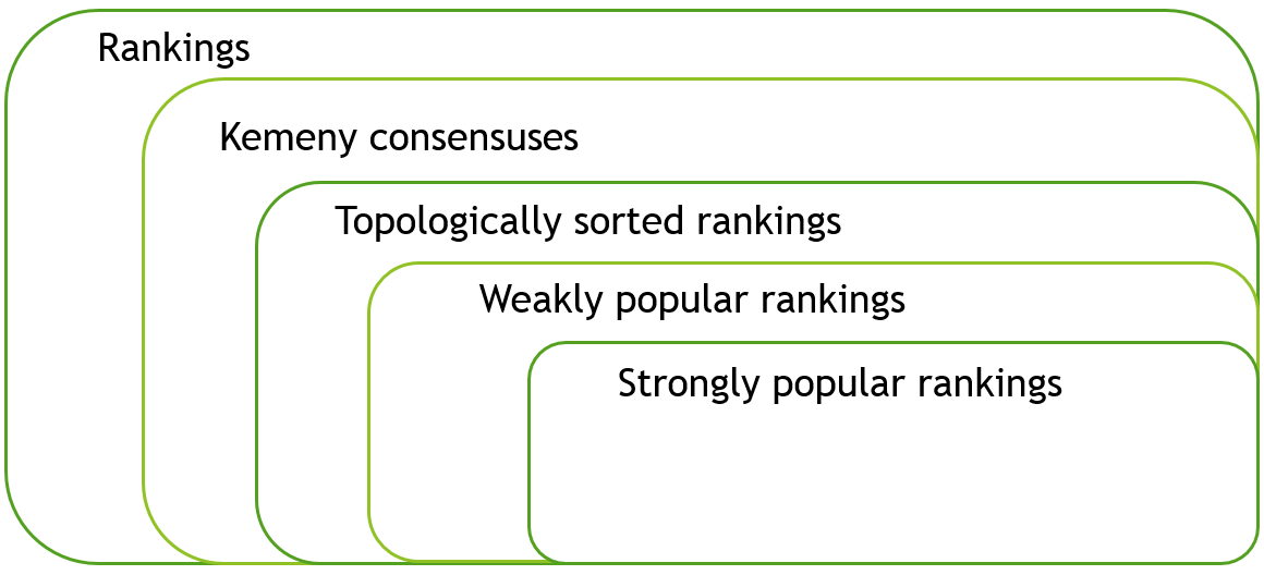
Figure 3: The hierarchy of various optimality notions for rankings as a Venn diagram. A Kemeny consensus always exists, but its subset of topologically sorted rankings might be empty.

3.2 Difference for six voters

Before presenting our example with $n=6$, we present a useful technical lemma. Let $(C_{1},\ldots,C_{k})$ be an ordered partition of $C$ into $k$ sets. We say that a ranking $\pi$ preserves $(C_{1},\ldots,C_{k})$ if it holds that rank${}_{\pi}[a]<$rank${}_{\pi}[b]$ whenever $a\in C_{i}$ and $b\in C_{j}$ for some $i<j$.

Lemma 3.3.

Let $(C_{1},\dots,C_{k})$ be an ordered partition of $C$ such that, for each $v\in V$, $\pi_{v}$ preserves $(C_{1},\dots,C_{k})$. Then for any ranking $\sigma$, there exists a ranking $\zeta$ such that, for each $v\in V,\zeta$ preserves $(C_{1},\dots,C_{k})$ and $v$ prefers $\zeta$ to $\sigma$ or abstains in the vote between them.

Proof 2.

Let $\tau_{i}$ be a ranking of the candidates in $C_{i}$. We denote by $\tau_{1}\tau_{2}\ldots\tau_{{\color[rgb]{0,0,0}k}}$ the ranking of the candidates $\cup_{i=1}^{{\color[rgb]{0,0,0}k}}C_{i}=C$, in which each candidate in $C_{i}$ is preferred to each candidate in $C_{j}$ whenever $i<j$, and candidates within a set $C_{i}$ are ranked according to $\tau_{i}$. Let $\zeta_{i}$ be the ranking on $C_{i}$ that orders candidates in $C_{i}$ according to their rank in $\sigma$, that is, $\operatorname{rank}_{\zeta_{i}}[a]<\operatorname{rank}_{\zeta_{i}}[b]$ if $\operatorname{rank}_{\sigma}[a]<\operatorname{rank}_{\sigma}[b]$. Let $\zeta:=\zeta_{1}\zeta_{2}\ldots\zeta_{k}$. So $\zeta$ preserves $(C_{1},\ldots,C_{k})$. Consider voter $v\in V$. If $v$ prefers $a$ to $b$, and $\zeta$ orders $b$ before $a$, then since by assumption $\pi_{v}$ preserves $(C_{1},\ldots,C_{k})$, it follows that $a,b\in C_{i}$ for some $1\leq i\leq m$. Since the relative order of candidates in $C_{i}$ is the same in $\zeta$ and $\sigma$ by construction, $\sigma$ also orders $b$ before $a$. In particular, every pair of candidates that contributes 1 to $K(\zeta,\pi_{v})$ also contributes 1 to $K(\sigma,\pi_{v})$. We conclude for any $v\in V$, it holds that $K(\zeta,\pi_{v})\leq K(\sigma,\pi_{v})$, as desired.

Theorem 3.4.

There exists a profile with six voters that has a weakly popular ranking which is not strongly popular.

Proof 3.

We prove this statement for the profile $P$ from Figure 1.

Claim 3.5.

$\sigma_{2}=[1,2,3],[4,5,6],[7,8,9]$ is weakly popular.

Proof 4.

Let $C_{1}=\{1,2,3\},C_{2}=\{4,5,6\},C_{3}=\{7,8,9\}$. Note that all voters preserve $(C_{1},C_{2},C_{3})$. By Lemma 3.3, in order to check if $\sigma_{2}$ is weakly popular it suffices to generate the $6^{3}$ rankings that preserve $(C_{1},C_{2},C_{3})$, and compare each of them to $\sigma_{2}$. We checked all of these rankings using program code, which is available from https://github.com/SonjaKrai/PopularRankingsExampleCheck. $\blacksquare$

Claim 3.6.

$\sigma_{2}=[1,2,3],[4,5,6],[7,8,9]$ is not strongly popular.

Proof 5.

Ranking $\sigma_{1}=[1,2,3],[5,6,4],\allowbreak[9,7,8]$ is more popular than $\sigma_{2}$ in the simple sense, because voters $v_{1},v_{2},v_{3}$ abstain, voter $v_{4}$ prefers $\sigma_{2}$ to $\sigma_{1}$, and finally, voters $v_{5}$ and $v_{6}$ prefer $\sigma_{1}$ to $\sigma_{2}$. A contains the detailed calculations that justify the preferences of each voter between $\sigma_{1}$ and $\sigma_{2}$. $\blacksquare$

This finishes the proof of our theorem.

We remark that Theorem 3.4 can be easily extended to $k>6$ voters, for even values of $k$, by adding $k-6$ voters to the profile $P$ from Figure 1, where half of the new voters have $\sigma_{1}$ as their ranking, and the other half of the new voters have $\sigma_{2}$ as their ranking.

For the sake of completeness, we also remark that the profile $P$ from Figure 1 has four further weakly popular rankings, each of which is strongly popular as well. For a profile that admits a weakly popular ranking but does not admit a strongly popular ranking, we refer to reader to B.

3.3 When are weakly and strongly popular rankings equivalent?

We now present a sufficient condition under which strong popularity follows from weak popularity. We start by showing that for a ranking $\pi$ that is not strongly popular, there is a condition under which we can compute a ranking that is also more popular than $\pi$ in the absolute sense.

Lemma 3.7.

If $\sigma_{1}$ is more popular than $\pi$ in the simple sense and the majority graph of the voters in $V_{\text{abs}}(\sigma_{1},\pi)$ is acyclic, then there is a ranking $\sigma_{2}$ that is more popular than $\pi$ in the absolute sense. Such a $\sigma_{2}$ can be computed in polynomial time.

Proof 6.

If $\pi$ is not a topologically sorted ranking then $\pi$ cannot be weakly popular by Observation 3.2. As in the proof of Lemma 2 in [35], we may construct a ranking $\sigma_{2}$ that is more popular than $\pi$ in the absolute sense. In particular, there must be $a,b$ such that $rank_{\pi}[b]<rank_{\pi}[a]$ and an absolute majority of voters in $V$ prefer $a$ to $b$. Let $\sigma_{2}$ be the ranking obtained by swapping $a$ and $b$. The proof of Lemma 2 in  [35] shows that $\sigma_{2}$ is preferred to $\pi$ by an absolute majority of voters who prefer $a$ to $b$. This shows that $\sigma_{2}$ is more popular in the absolute sense. Hence suppose that $\pi$ is a topologically sorted ranking. Furthermore, if $V_{\text{abs}}(\sigma_{1},\pi)=\emptyset$, then $\sigma_{1}$ is preferred to $\pi$ by an absolute majority of all voters, and thus the theorem is proved by taking $\sigma_{2}:=\sigma_{1}$.

From here on we therefore assume that $\pi$ is topologically sorted and that $V_{\text{abs}}(\sigma_{1},\pi)\neq\emptyset$. Let $D(\sigma_{1},\pi)\neq\emptyset$ be the set of pairs of candidates that are ordered differently in $\sigma_{1}$ and $\pi$.

Claim 3.8.

If $v\in V_{\text{abs}}(\sigma_{1},\pi)$, then $v$ agrees with $\pi$ on the order of exactly half of the pairs in $D(\sigma_{1},\pi)$, and disagrees on the other half. In particular, $|D(\sigma_{1},\pi)|$ is even.

Proof 7.

Any pair of candidates $\{a,b\}$ such that $\sigma_{1}$ and $\pi$ agree on the order $(a,b)$, adds $1$ to both $K(\pi_{v},\sigma_{1})$ and $K(\pi_{v},\pi)$ if $\pi_{v}$ has them in the relative order $(b,a)$, and adds 0 to both otherwise. So to be impartial, i.e. to have $K(\pi_{v},\sigma_{1})=K(\pi_{v},\pi)$, voter $v\in V_{\text{abs}}(\sigma_{1},\pi)$ must agree with $\sigma_{1}$ on the order of exactly half of the pairs in $D(\sigma_{1},\pi)$, and disagree on the other half. So $|D(\sigma_{1},\pi)|$ must be even. $\blacksquare$

Claim 3.9.

There exist consecutive candidates $(a^{*},b^{*})$ in $\sigma_{1}$ such that at least half of the voters in $V_{\text{abs}}(\sigma_{1},\pi)$ prefer $b^{*}$ to $a^{*}$.

Proof 8.

Assume the contrary, i.e. that for any two consecutive candidates in $\sigma_{1}$, an absolute majority of voters in $V_{\text{abs}}(\sigma_{1},\pi)$ agree with $\sigma_{1}$. For an arbitrary pair of candidates $\{a,b\}$, at least half of the voters in $V_{\text{abs}}(\sigma_{1},\pi)$ must then also agree with their order in $\sigma_{1}$, as otherwise this would imply a directed cycle in their majority graph, which is acyclic by assumption.

Since $\sigma_{1}\neq\pi$, there is some ordered pair $(a^{*},b^{*})$ that is consecutive in $\sigma_{1}$ and $b^{*}$ is ordered somewhere before $a^{*}$ in $\pi$, that is $\operatorname{rank}_{\pi}[b^{*}]<\operatorname{rank}_{\pi}[a^{*}]$. Note that $(a^{*},b^{*})\in D(\sigma_{1},\pi)$. In particular, by our starting assumption, an absolute majority of voters in $V_{\text{abs}}(\sigma_{1},\pi)$ agrees with $\sigma_{1}$ on the order $(a^{*},b^{*})$ and hence disagrees with $\pi$.

We now introduce the indicator variable $I_{v,\pi,\{a,b\}}$, which is set to 1 if $\pi_{v}$ and $\pi$ disagree on the order of candidates $a$ and $b$, and it is set to 0 otherwise. We sum up the disagreements of voters in $V_{\text{abs}}(\sigma_{1},\pi)$ with $\pi$ over pairs in $D(\sigma_{1},\pi)$ and obtain a contradiction.

$$|V_{\text{abs}}(\sigma_{1},\pi)|\frac{|D(\sigma_{1},\pi)|}{2} = \sum_{\{a,b\}\in D(\sigma_{1},\pi)}\sum_{v\in V_{\text{abs}}(\sigma_{1},\pi)}I_{v,\pi,\{a,b\}}$$ (1)

$$> \sum_{\{a,b\}\in D(\sigma_{1},\pi)}\frac{|V_{\text{abs}}(\sigma_{1},\pi)|}{2}$$ (2)

$$= |V_{\text{abs}}(\sigma_{1},\pi)|\frac{|D(\sigma_{1},\pi)|}{2}$$ (3)

The right-hand side of Line 1 is a formulation of disagreements in terms of the indicator variable. Due to Claim 3.8, the number of disagreements that abstaining voters have with $\pi$ is exactly half of $|D(\sigma_{1},\pi)|$, expressed on the left-hand side of Line 1. The inequality in Line 2 follows because for all pairs in $D(\sigma_{1},\pi)$, at least half of the abstaining voters disagree with $\pi$, and, additionally, there exists a pair $\{a^{*},b^{*}\}$ such that an absolute majority of voters in $V_{\text{abs}}(\sigma_{1},\pi)$ disagree with $\pi$, as we proved above. Finally, reordering the terms as in Line 3 leads back to the same formula as on the left-hand side in Line 1, creating a contradiction. $\blacksquare$

The pair of candidates $(a^{*},b^{*})$ in Claim 3.9 leads us to a suitable ranking $\sigma_{2}$. Let $\sigma_{2}$ be the ranking we get from $\sigma_{1}$ by the swap $(a^{*},b^{*})\rightarrow(b^{*},a^{*})$. We now prove Claims 3.10 and 3.11, which we will use to show that two groups of voters prefer $\sigma_{2}$ to $\pi$, and that these two groups constitute an absolute majority of all voters.

Claim 3.10.

All voters $v\in V_{\text{abs}}(\sigma_{1},\pi)$ who prefer $b^{*}$ to $a^{*}$ also prefer $\sigma_{2}$ to $\pi$.

Proof 9.

If $v\in V_{\text{abs}}(\sigma_{1},\pi)$ prefers $b^{*}$ to $a^{*}$, then the following holds.

$$K(\pi_{v},\sigma_{2}) = K(\pi_{v},\sigma_{1})-1$$ (4)

$$< K(\pi_{v},\sigma_{1})$$ (5)

$$= K(\pi_{v},\pi)$$ (6)

Line 4 is true, because $\sigma_{2}$ is obtained from $\sigma_{1}$ by performing a swap that is good for voter $v$. The equality in Line 6 holds since $v$ abstains between $\sigma_{1}$ and $\pi$. Line 6 together with the inequality in Line 5 prove the claim. $\blacksquare$

The second group of voters we investigate consists of voters who prefer $\sigma_{1}$ to $\pi$. This group by assumption makes up an absolute majority of the non-abstaining voters $V\setminus V_{\text{abs}}(\sigma_{1},\pi)$. Let voter $v$ belong to this group.

Claim 3.11.

If $K(\pi_{v},\sigma_{1})<K(\pi_{v},\pi)$ for voter $v\in V\setminus V_{\text{abs}}(\sigma_{1},\pi)$, then $K(\pi_{v},\sigma_{1})+2\leq K(\pi_{v},\pi)$.

Proof 10.

Only the pairs in $D(\sigma_{1},\pi)$ contribute differently to $K(\pi_{v},\sigma_{1})$ and to $K(\pi_{v},\pi)$. In particular, a pair in $D(\sigma_{1},\pi)$ adds $1$ to either $K(\pi_{v},\sigma_{1})$ or $K(\pi_{v},\pi)$, and $0$ to the other. Using this we can see that if $k$ is the number of pairs on whose order $\sigma_{1}$ and $\pi$ agree, but $\pi_{v}$ disagrees, then $K(\pi_{v},\sigma_{1})+K(\pi_{v},\pi)=|D(\sigma_{1},\pi)|+2k$, which is even by Claim 3.8. Since $K(\pi_{v},\sigma_{1})<K(\pi_{v},\pi)$ by assumption and their sum $|D(\sigma_{1},\pi)|+2k$ is even, $K(\pi_{v},\sigma_{1})+2\leq K(\pi_{v},\pi)$ must hold. $\blacksquare$

Since a swap of consecutive candidates in a ranking can increase the distance to any other ranking by at most one, Claim 3.11 implies that for any voter $v$ who prefers $\sigma_{1}$ to $\pi$, the following holds:

$$K(\pi_{v},\sigma_{2})\leq K(\pi_{v},\sigma_{1})+1<K(\pi_{v},\pi).$$

We conclude that voters who prefer $\sigma_{1}$ to $\pi$ also prefer $\sigma_{2}$ to $\pi$.

Claims 3.9 and 3.10 imply that at least half of the voters in $V_{\text{abs}}(\sigma_{1},\pi)$ prefer $\sigma_{2}$ to $\pi$, and Claim 3.11 proves that more than half of the voters outside of $V_{\text{abs}}(\sigma_{1},\pi)$ prefer $\sigma_{2}$ to $\pi$. The two sets of voters thus constitute an absolute majority of all voters who prefer $\sigma_{2}$ to $\pi$.

By rephrasing Lemma 3.7, we obtain the following.

Theorem 3.12.

If ranking $\pi$ is weakly popular, and for any ranking $\sigma$, $V_{\text{abs}}(\sigma,\pi)$ has an acyclic majority graph, then $\pi$ is also strongly popular. Furthermore, if $V_{\text{abs}}(\sigma,\pi)$ has an acyclic majority graph for each weakly popular ranking $\pi$ and any ranking $\sigma$ for a profile $P$, then weakly and strongly popular rankings for $P$ coincide.

Observation 3.13.

The acyclicity condition for the majority graph of the abstaining voters in Lemma 3.7 and Theorem 3.12 is necessary.

Proof 11.

We construct an example to demonstrate that there is a profile and rankings $\sigma_{1}$, $\sigma_{2}$ such that the majority graph of the voters in $V_{\text{abs}}(\sigma_{1},\sigma_{2})$ is cyclic (contradicting our assumption in Lemma 3.7 and Theorem 3.12), and $\sigma_{2}$ is weakly popular but not strongly popular.

Consider the profile described in Figure 1 with $\sigma_{1}=[1,2,3],[5,6,4],[9,7,8]$ and $\sigma_{2}=[1,2,3],[4,5,6],[7,8,9]$, as in the proof of Theorem 3.4. Notice that there are three directed cycles in the majority graph of the three abstaining voters $v_{1},v_{2},v_{3}$: one for candidates $1,2,3$, one for candidates $4,5,6$ and one for candidates $7,8,9$. So the abstaining voters have a cyclic majority graph.

As shown by Claims 3.5 and 3.6 in the proof of Theorem 3.4, $\sigma_{2}$ is weakly popular but not strongly popular, since $\sigma_{1}$ is more popular than $\sigma_{2}$ in the simple sense. Therefore, this example justifies the necessity of the acyclicity condition for the majority graph of the abstaining voters in Lemma 3.7 and Theorem 3.12.

3.4 At most five voters

From Lemma 3.7 we can deduce that for a small number of voters, the two notions of popularity are equivalent. This is due to the fact that we need at least three abstaining voters in order for $V_{\text{abs}}(\sigma,\pi)$ to have a cyclic majority graph.

Theorem 3.14.

A ranking $\sigma$ is weakly popular for a profile $P$ with at most five voters if and only if it is strongly popular for $P$.

Proof 12.

From Observation 3.2 we know that strongly popular rankings are also weakly popular, which allows us to concentrate only on one direction of the statement, namely that if a ranking is not strongly popular, then it also cannot be weakly popular. Let us assume that ranking $\pi$ is not strongly popular. By definition there exists a ranking $\sigma$ that is preferred to $\pi$ by an absolute majority of non-abstaining voters $V\setminus V_{\text{abs}}(\sigma,\pi)\neq\emptyset$.

If at least one voter prefers $\pi$ to $\sigma$, then at least two voters must prefer $\sigma$ to $\pi$, and the remaining at most two abstaining voters can only form an acyclic majority graph. From this it follows by Lemma 3.7 that $\pi$ is not weakly popular.

On the other hand, if no voter prefers $\pi$ to $\sigma$, then $K(\pi_{v},\sigma)\leq K(\pi_{v},\pi)$ holds for all voters. For $V\setminus V_{\text{abs}}(\sigma,\pi)\neq\emptyset$, by assumption there is a voter $v^{*}$ who prefers $\sigma$ to $\pi$, that is, for whom $K(\pi_{v^{*}},\sigma)<K(\pi_{v^{*}},\pi)$. We thus have $\sum_{i=1}^{n}K(\pi_{v_{i}},\sigma)<\allowbreak\sum_{i=1}^{n}K(\pi_{v_{i}},\pi)$. This means that $\pi$ is not a Kemeny consensus and by Observation 3.2, $\pi$ is not weakly popular.

4 On the complexity of $k$-wurv and $k$-surv

In this section, we analyse the complexity of the verification problems for the two popularity notions. We prepare for this by giving a sufficient condition for weak popularity in Section 4.1. This condition will then be used in Section 4.2, where we prove the polynomial solvability of both problems in the case of $k\leq 3$. For $4\leq k\leq 5$, we reach the same conclusion in Section 4.3, however, only for special profiles. Then, in Section 4.4, $\NP$-hardness is proved for $k=6$.

4.1 A sufficient condition for wurv

We call a ranking $\pi$ $c$-sorted for $0<c\leq 1$ if for all pairs of candidates $\{a,b\}$ with $\operatorname{rank}_{\pi}[a]<\operatorname{rank}_{\pi}[b]$, at least a $c$-fraction of the voters prefers $a$ to $b$. A ranking $\pi$ is topologically sorted if and only if it is $\frac{1}{2}$-sorted. In [35], van Zuylen et al. show that even a topologically sorted ranking is not necessarily weakly popular. Here we ask for which constant $\frac{1}{2}<c\leq 1$ does this negative result change to a positive result, guaranteeing a no answer for $k$-wurv. (Note that we do not consider the case where $c<\frac{1}{2}$, since any $c$-popular ranking cannot be topologically sorted and hence cannot be weakly popular by Observation 3.2.)

Theorem 4.1.

$c=\frac{3}{4}$ is the smallest constant ($\frac{1}{2}<c\leq 1$)for which the following holds: If a profile $P$ admits a $c$-sorted ranking $\pi$, then $\pi$ is weakly popular.

Proof 13.

We first show that any $\frac{3}{4}$-sorted ranking is weakly popular.

Claim 4.2.

Let $P$ be a profile and $\pi$ be a $\frac{3}{4}$-sorted ranking for $P$. Then $\pi$ is weakly popular.

Proof 14.

Let $\sigma$ be any ranking different from $\pi$. We will show that there is no voter set of cardinality $\lfloor\frac{n}{2}\rfloor+1$, in which every voter prefers $\sigma$ to $\pi$. Let $V^{\prime}$ be an arbitrary set of $\lfloor\frac{n}{2}\rfloor+1$ voters. On the bubble swap path $\pi_{0}:=\pi,\pi_{1},\ldots\pi_{k}:=\sigma$ from $\pi$ to $\sigma$, each swap $\pi_{i}\rightarrow\pi_{i+1}$ is bad for at least a $\frac{3}{4}$-fraction of voters in $V$. So it must be bad for at least

$${\color[rgb]{0,0,0}\left\lfloor\frac{n}{2}\right\rfloor}+1-\frac{n}{4}\geq\frac{|V^{\prime}|}{2}$$

voters in $V^{\prime}$. Hence for a swap $\pi_{i}\rightarrow\pi_{i+1}$, we have that $\sum_{v\in V^{\prime}}(K(\pi_{i+1},\pi_{v})-K(\pi_{i},\pi_{v}))\geq 0$. Summing over all swaps we get a telescoping sum that reduces to

$$\sum_{v\in V^{\prime}}(K(\sigma,\pi_{v})-K(\pi,\pi_{v}))\geq 0.$$

In particular, not every $v\in V^{\prime}$ can prefer $\sigma$ to $\pi$. Since $V^{\prime}$ was an arbitrary set of size $\lfloor\frac{n}{2}\rfloor+1$, no voter set of at least this size can prefer $\sigma$ to $\pi$, and thus, $\pi$ must be weakly popular. $\blacksquare$

We now show that in fact $c=\frac{3}{4}$ is tight, meaning that for any $\frac{1}{2}<$ $c<\frac{3}{4}$, we can construct a profile $P$ and a $c$-sorted ranking $\pi$ such that $\pi$ is not weakly popular for $P$.

Claim 4.3.

For arbitrary $\frac{1}{2}\leq c<\frac{3}{4}$ there exists a profile $P$ and a c-sorted ranking $\pi$ that is not weakly popular.

Proof 15.

Let $c=\frac{3}{4}-\varepsilon$ for some $\frac{1}{4}\geq\varepsilon>0$. Next, choose $j$ such that $j\geq\frac{1}{4\varepsilon}$. We will create profile $P$ with $4j$ voters and $4j+2$ candidates. Then it holds that $(\frac{1}{4}+\varepsilon)|V|\geq j+1$.

Each voter’s ranking involves $2j+1$ blocks, where block $i$ comprises candidates $\{2i-1,2i\}$ ($1\leq i\leq 2j+1$). We say that block $i$ is increasing if it is in the form $[2i-1,2i]$ and it is decreasing if it is in the form $[2i,2i-1]$.

We firstly create a set $V_{1}$ of $2j-1$ voters, and each voter in $V_{1}$ has only increasing blocks, meaning that their ranking is $\pi=[1,2],[3,4],\ldots,$ [4$j$+1,4$j$+2]. The set $V_{2}$ comprises the $2j+1$ remaining voters, and their set of rankings is constructed as follows. The $i$th voter in $V_{2}$ ($1\leq i\leq 2j+1$) has blocks $i\mod(2j+1)$ to $(i+j)\mod(2j+1)$ decreasing, whilst all other blocks are increasing. This construction is illustrated in Figure 4 for the case that $j=3$. This construction is similar to the one in [35, Lemma 3].

$\pagecolor{C1}[2,1]$	$\pagecolor{C1}[4,3]$	$\pagecolor{C1}[6,5]$	$\pagecolor{C1}[8,7]$	$[9,10]$	$[11,12]$	$[13,14]$
$\pagecolor{white}[1,2]$	$\pagecolor{C1}[4,3]$	$\pagecolor{C1}[6,5]$	$\pagecolor{C1}[8,7]$	$\pagecolor{C1}[10,9]$	$[11,12]$	$[13,14]$
$\pagecolor{white}[1,2]$	$[3,4]$	$\pagecolor{C1}[6,5]$	$\pagecolor{C1}[8,7]$	$\pagecolor{C1}[10,9]$	$\pagecolor{C1}[12,11]$	$[13,14]$
$\pagecolor{white}[1,2]$	$[3,4]$	$[5,6]$	$\pagecolor{C1}[8,7]$	$\pagecolor{C1}[10,9]$	$\pagecolor{C1}[12,11]$	$\pagecolor{C1}[14,13]$
$\pagecolor{C1}[2,1]$	$[3,4]$	$[5,6]$	$[7,8]$	$\pagecolor{C1}[10,9]$	$\pagecolor{C1}[12,11]$	$\pagecolor{C1}[14,13]$
$\pagecolor{C1}[2,1]$	$\pagecolor{C1}[4,3]$	$[5,6]$	$[7,8]$	$[9,10]$	$\pagecolor{C1}[12,11]$	$\pagecolor{C1}[14,13]$
$\pagecolor{C1}[2,1]$	$\pagecolor{C1}[4,3]$	$\pagecolor{C1}[6,5]$	$[7,8]$	$[9,10]$	$[11,12]$	$\pagecolor{C1}[14,13]\par\par$

Figure 4: The rankings of the voters $V_{2}$, as described in the proof of Claim 4.3, for the special case where $j=3$. The decreasing blocks are highlighted.

For each $\{2i-1,2i\}$ for $1\leq i\leq 2j+1$, every $v\in V_{1}$ agrees with this pair and also exactly $j$ of the voters in $V_{2}$ agree with it. In total, $3j-1$ voters thus agree with this pair. This gives the following fraction of all voters:

$$\frac{3j-1}{4j}=\frac{3}{4}-\frac{1}{4j}\geq\frac{3}{4}-\varepsilon.$$

It is trivial to see for all other pairs of voters $\{a,b\}$ that if $a<b$ then all voters prefer $a$ to $b$. Hence in particular $\pi$ is $\left(\frac{3}{4}-\varepsilon\right)$-sorted.

We now show that ranking $\sigma=[2,1],[4,3],\ldots[4j+2,4j+1]$ is preferred to $\pi$ by an absolute majority of all voters, namely by all $2j+1$ voters in $V_{2}$. Each voter in $V_{2}$ has exactly $j+1$ blocks with decreasing order and $j$ blocks with increasing order. Therefore, each of them would rather have all pairs in decreasing order than all pairs in increasing order. $\blacksquare$

Theorem 4.1 is thus established.

As an aside, following on from Theorem 4.1, it is natural to ask about the existence of $c$-popular rankings: rankings that are preferred to all other rankings by some $c$-fraction of voters.

Theorem 4.4.

There is a profile that does not admit a c-popular ranking for any $c>0$.

Proof 16.

Let $n=\lceil\frac{1}{c}\rceil+1$. We exhibit a profile of $n$ voters over $n$ candidates, such that for any ranking $\pi$, there exists another ranking $\sigma$ such that $n-1$ voters prefer $\sigma$ to $\pi$ and only one voter prefers $\pi$ to $\sigma$. This implies that $\pi$ cannot be preferred to any other ranking by a $c$-fraction of the voters, since $\frac{1}{n}<c$.

Consider the extended Condorcet paradox, i.e. $n$ voters with rankings of $n$ candidates as follows:

$\pi_{v_{1}}=$	$1,2,$	$\ldots,$	$n-1,n$
$\pi_{v_{2}}=$	$2,3,$	$\ldots,$	$n,1$
⋮
$\pi_{v_{n}}$=	$n,1,$	$\ldots,$	$n-2,n-1$

Let $\pi$ be an arbitrary ranking of the $n$ candidates. For each ordered pair $(a,b)$ in the set $A:=\{(1,2),(2,3),\ldots(n-1,n),(n,1)\}$, exactly $n-1$ voters of the above instance agree with $(a,b)$. We also know that there must be at least one ordered pair in $A$ with which the ranking $\pi$ disagrees. Let $(a,b)$ be such a pair, so $\pi$ prefers $b$ to $a$, but $n-1$ voters prefer $a$ to $b$.

Let $\sigma$ be the ranking obtained from $\pi$ by swapping $b$ and $a$. Let $d$ be a candidate ranked between $b$ and $a$ in $\pi$. Each voter $v$ who prefers $a$ to $b$ must also prefer $a$ to $d$ or prefer $d$ to $b$. So since $\operatorname{rank}_{{\color[rgb]{0,0,0}\pi}}[b]<\operatorname{rank}_{{\color[rgb]{0,0,0}\pi}}[{\color[rgb]{0,0,0}d}]<\operatorname{rank}_{{\color[rgb]{0,0,0}\pi}}[a]$ together the pairs $(a,{\color[rgb]{0,0,0}d})$ and $({\color[rgb]{0,0,0}d},b)$ add at least $1$ to $K(\pi_{v},\pi)$. Since $\operatorname{rank}_{{\color[rgb]{0,0,0}\sigma}}[a]<\operatorname{rank}_{{\color[rgb]{0,0,0}\sigma}}[{\color[rgb]{0,0,0}d}]<\operatorname{rank}_{{\color[rgb]{0,0,0}\sigma}}[b]$, at most one of the pairs $(a,{\color[rgb]{0,0,0}d})$ and $({\color[rgb]{0,0,0}d},b)$ adds $1$ to $K(\pi_{v},\sigma)$. Pair $(a,b)$ adds $1$ to $K(\pi_{v},\pi)$ and $0$ to $K(\pi_{v},\sigma)$. From the definition of $\sigma$, it follows that $K(\pi_{v},\sigma)<K(\pi_{v},\pi)$ for each voter who prefers $a$ to $b$ and there are $n-1$ such voters $v$.

4.2 Polynomial-time solvability for $k\leq 3$

Since we have shown in Theorem 3.14 that weak and strong popularity are equivalent notions for $k\leq 5$, we will refer to them as popularity if $k\leq 5$.

We first show that for $k\leq 3$, the problems $k$-wurv and $k$-surv are polynomial-time solvable. We establish this by proving that for at most three voters, the set of topologically sorted rankings coincides with the set of popular rankings. Since verifying whether a given ranking is topologically sorted can be carried out in polynomial time, $k$-wurv and $k$-surv turn out to be polynomial-time solvable for $k=2,3$.

Lemma 4.5.

Given a profile of two voters, a ranking is popular if and only if it is topologically sorted.

Proof 17.

From Observation 3.2 we know that all popular rankings must be topologically sorted. Let $D(\pi_{v_{1}},\pi_{v_{2}})$ be the set of pairs of candidates $\{a,b\}$ that $\pi_{v_{1}}$ and $\pi_{v_{2}}$ order differently. Consider any ranking $\pi$. Each pair $\{a,b\}\in D(\pi_{v_{1}},\pi_{v_{2}})$ adds $1$ to either $K(\pi_{v_{1}},\pi)$ or $K(\pi_{v_{2}},\pi)$. From this follows that

$$|D(\pi_{v_{1}},\pi_{v_{2}})|\leq K(\pi_{v_{1}},\pi)+K(\pi_{v_{2}},\pi).$$

If $\sigma$ is a topologically sorted ranking, then by definition there is no pair of candidates $\{a,b\}$ that adds $1$ to both $K(\pi_{v_{1}},\sigma)$ and $K(\pi_{v_{2}},\sigma)$. Thus, $K(\pi_{v_{1}},\sigma)+K(\pi_{v_{2}},\sigma)=|D(\pi_{v_{1}},\pi_{v_{2}})|$. If $\pi$ is preferred to $\sigma$ by an absolute majority, then both voters prefer $\pi$ to $\sigma$, which leads to

$$|D(\pi_{v_{1}},\pi_{v_{2}})| \leq K(\pi_{v_{1}},\pi)+K(\pi_{v_{2}},\pi)$$

$$< K(\pi_{v_{1}},\sigma)+K(\pi_{v_{2}},\sigma)$$

$$= |D(\pi_{v_{1}},\pi_{v_{2}})|.$$

Since this is a contradiction, $\sigma$ must be weakly popular. By Theorem 3.14, $\sigma$ is also strongly popular.

Lemma 4.6.

Given a profile $P$ of three voters, a ranking is popular if and only if it is topologically sorted.

Proof 18.

Just as for the $k=2$ case, Observation 3.2 implies here as well that all popular rankings must be topologically sorted. Let $\pi$ be a topologically sorted ranking for $P$. Note that whenever $\operatorname{rank}_{\pi}[a]~{}<~{}\operatorname{rank}_{\pi}[b]$ holds for candidates $a$ and $b$, at least half of the voters, that is, at least two voters prefer $a$ to $b$. So for any two voters, at least one of them prefers $a$ to $b$, implying that $\pi$ is also topologically sorted for any two of the three voters. In particular, $\pi$ is weakly popular for any two voters by Lemma 4.5, showing that there is no ranking that they both prefer to $\pi$. Hence $\pi$ must be weakly popular for $P$ and by Theorem 3.14, also strongly popular.

Lemmas 4.5 and 4.6 lead to the following result regarding the complexity of $k$-wurv and $k$-surv for $k\leq 3$, and the complexity of finding a popular ranking or reporting that none exists in the case that $k\leq 3$.

Theorem 4.7.

For $k\leq 3$, $k$-wurv and $k$-surv are solvable in $O(m^{2}n)$ time. Moreover for $k\leq 3$, we can find a popular ranking or report that none exists in $O(m^{2}n)$ time.

Proof 19.

Let $D$ denote the majority graph for the given profile $P$. Lemmas 4.5 and 4.6 state that a given ranking is popular if and only if it is topologically sorted for $P$. Moreover a topologically sorted ranking exists if and only if $D$ is acyclic.

To establish the time complexity, clearly it is trivial to construct in $O(m)$ time for each voter $v_{i}$ a data structure that allows us to check in $O(1)$ time whether $v_{i}$ prefers $a$ to $b$, for any pair of candidates $a,b$. Thus the $m\times m$ matrix $N$, where $N(a,b)$ gives the number of voters who prefer candidate $a$ to candidate $b$ (i.e. $N(a,b)=|V(a,b)|$), can be constructed in $O(m^{2}n)$ time.

Using $N$, we can then compute $D$ in $O(m^{2})$ time. To find a popular ranking or report that none exists, we can check in $O(m^{2})$ time whether $D$ is acyclic, and if so, construct a topological ordering of $D$ in the same time complexity. Alternatively, for a given ranking $\pi$, clearly we can check whether $\pi$ is topologically sorted for $P$ in $O(m^{2})$ time. The overall time complexity is thus $O(m^{2}n)$ for both the verification and search algorithms.

4.3 Equivalence of the cases $k=4$ and $k=5$

If we have four or five voters, it turns out a topologically sorted ranking may not be popular anymore. In the case of an acyclic tournament as the majority graph, finding and verifying a popular ranking are both polynomial-time solvable. We further show that $4$-wurv ($4$-surv) in general is polynomial-time solvable if and only if $5$-wurv ($5$-surv) is.

Lemma 4.8.

If a profile $P$ of four voters has an acyclic tournament as its majority graph, then the unique topologically sorted ranking is the unique popular ranking.

Proof 20.

Since the majority graph of $P$ is a tournament, the unique topologically sorted ranking $\pi$ is $\frac{3}{4}$-sorted. The lemma then follows from Theorem 4.1 and Observation 3.2.

Lemma 4.9.

Let $P$ be a profile of four voters with an acyclic majority graph, and let $\pi$ be a ranking for $P$ that is popular for at least one of the profiles formed by three of the voters. Then $\pi$ is popular for $P$.

Proof 21.

Let $\pi$ be popular for the profile $(\pi_{v_{1}},\pi_{v_{2}},\pi_{v_{3}})$. Then by definition there exists no ranking $\sigma$ that is preferred by two of $v_{1},v_{2},v_{3}$, as this would contradict the fact that $\pi$ is weakly popular for the profile $(\pi_{v_{1}},\pi_{v_{2}},\pi_{v_{3}})$ by Theorem 3.14. In particular, there does not exist a ranking $\sigma$ preferred by an absolute majority of $v_{1},v_{2},v_{3},v_{4}$, as this would require at least three voters and hence at least $2$ of $v_{1},v_{2},v_{3}$. We conclude that $\pi$ is weakly popular and hence popular for $P$.

We now present an example in which there is ranking $\pi$ that is not topologically sorted such that $\pi$ is more popular than a topologically sorted ranking.

Observation 4.10.

Given a profile of four voters with an acyclic majority graph, a ranking that is not topologically sorted can be more popular than a topologically sorted ranking.

Proof 22.

Consider the following profile with $n=4$ and $m=10$.

$$\pi_{v_{1}} =[1,2],[3,4],[5,6],[7,8],[9,10]$$

$$\pi_{v_{2}} =[1,2],[4,3],[6,5],[7,8],[10,9]$$

$$\pi_{v_{3}} =[1,2],[4,3],[6,5],[8,7],[9,10]$$

$$\pi_{v_{4}} =[2,1],[3,4],[5,6],[8,7],[10,9]$$

It is easy to verify that $\pi_{v_{1}}$ is a topologically sorted ranking of $P$. However, $\sigma=[2,1],[4,3],[6,5],[8,7],[10,9]$ is preferred by $v_{2}$, $v_{3}$, and $v_{4}$ to $\pi_{v_{1}}$, since $K(\pi_{v_{i}},\pi_{v_{1}})=3$ and $K(\pi_{v_{i}},\sigma)=2$ for $2\leq i\leq 4$. Since an absolute majority of voters prefer candidate $1$ to candidate $2$, $\sigma$ is not topologically sorted. For the sake of completeness, we remark that the topologically sorted ranking $[1,2],[4,3],[6,5],[8,7],[10,9]$ is popular.

We now discuss a family of strongly related decision problems called $k$-all-closer-ranking, which will come useful when establishing results for the cases $k=4$ and $k=5$. For a profile with $k$ voters and a given ranking $\pi$, we ask whether there is a ranking that all the voters prefer to $\pi$.

The next theorem reveals some features of this problem.

Theorem 4.11.

Given a profile $P=(\pi_{v_{1}},\pi_{v_{2}},\pi_{v_{3}})$ with an acyclic majority graph, we can decide in polynomial time if there exists a ranking preferred by all voters to a given ranking $\pi$ and if it does, output it.

Proof 23.

We start with two technical observations that will come in handy later in our proof.

Observation 4.12.

If $K(\sigma,{\color[rgb]{0,0,0}\pi_{v_{i}}})>0$— for a voter ${\color[rgb]{0,0,0}v_{i},1\leq i\leq 3}$ and a ranking $\sigma$, then there exists a swap in $\sigma$ that is good for $v_{i}$.

Proof 24.

Suppose there is no swap in $\sigma$ that is good for $v_{i}$. So $\sigma$ is a topologically sorted ranking for $v_{i}$, and for one voter this means ${\color[rgb]{0,0,0}\pi_{v_{i}}}=\sigma$, i.e. $K(\sigma,{\color[rgb]{0,0,0}\pi_{v_{i}}})=0$. $\blacksquare$

Observation 4.13.

Let $\pi$ be a ranking such that there is no swap in $\pi$ that is good for both $v_{i}$ and $v_{j}$, where $1\leq i,j\leq 3$. Then there is no ranking $\sigma$ preferred to $\pi$ by both $v_{i}$ and $v_{j}$.

Proof 25.

Since there is no swap in $\pi$ that is good for both $v_{i}$ and $v_{j}$, $\pi$ is a topologically sorted ranking for $v_{i}$ and $v_{j}$. By Lemma 4.5 this means that $\pi$ is weakly popular for the sub-profile comprising $v_{i}$ and $v_{j}$, so there exists no ranking preferred by an absolute majority, that is, preferred by both voters. $\blacksquare$

We are now ready to proceed to the main part of the proof. First, note that we can check in polynomial time whether $\pi$ is topologically sorted for any two of the voters and hence by Lemma 4.5 whether there is a ranking that they both prefer. Clearly if there is a pair of voters such that no ranking exists that is preferred to $\pi$ by both voters, then there is no ranking preferred to $\pi$ by all three voters. So we may assume that for any two of the three voters there is a ranking they both prefer to $\pi$.

Second, note that since the number of voters is odd, the majority graph is a tournament. First we compute the unique topologically sorted ranking $\sigma$ of $P$ in polynomial time [24]. We distinguish four cases, based on how many of the three voters prefer $\sigma$ to $\pi$, which can be checked in polynomial time.

Case 1: If $\sigma$ is preferred to $\pi$ by all three voters, then we are done.

Case 2: Suppose that two of the voters, without loss of generality $v_{1}$ and $v_{2}$, prefer $\sigma$ to $\pi$. Let $d_{i}=K(\pi,\pi_{v_{i}})-K(\sigma,\pi_{v_{i}})$ for $i\in\{1,2\}$. Then $d_{i}\geq 1$ for $i\in\{1,2\}$. Without loss of generality assume that $d_{1}\leq d_{2}$. Also let $d_{3}=K(\sigma,\pi_{v_{3}})-K(\pi,\pi_{v_{3}})$. Then $d_{3}\geq 0$. Let $\pi_{0}:=\pi,\ldots,\pi_{k}:=\sigma$ be the bubble sort swap path from $\pi$ to $\sigma$.

Claim 4.14.

For the above defined distances, $d_{1}-d_{3}\geq 2$ and similarly, $d_{2}-d_{3}\geq 2$ hold.

Proof 26.

Firstly, no swap in the bubble sort path is bad for both $v_{1}$ and $v_{3}$, since every swap $\pi_{i}\rightarrow\pi_{i+1}$ that is bad for $v_{3}$ must be good for both $v_{2}$ and $v_{1}$, because $\sigma$ is the topologically sorted ranking of $P$. If there is no swap that is good for both $v_{1}$ and $v_{3}$, then there cannot exist a ranking preferred to $\pi$ by all voters, since there cannot exist a ranking preferred by both $v_{1}$ and $v_{3}$ by Observation 4.13. So there is at least one swap in the bubble sort path that is good for both $v_{1}$ and $v_{3}$. This swap adds $1$ to $d_{1}$ and subtracts $1$ from $d_{3}$, i.e. it adds $1$ to $-d_{3}$. By the previous argument, any other swap is good for at least one of $v_{1}$ and $v_{3}$, adding at least $0$ to $d_{1}-d_{3}$. It follows that $d_{1}-d_{3}\geq 2$ and since $d_{2}\geq d_{1}$, it follows that the same argument also implies $d_{2}-d_{3}\geq 2$. $\blacksquare$

We now show how to transform $\sigma$ to a ranking that is preferred by all three voters to $\pi$ if and only if such a ranking exists.

Procedure
Let $\sigma_{0}=\sigma$. In the $i$th round we search for a swap in $\sigma_{i-1}$ that is good for $v_{3}$ and if found, perform the swap to obtain $\sigma_{i}$ for $i\geq 1$. Otherwise we output an error message. We stop the procedure in round $i=d_{3}+1$ and output $\sigma_{d_{3}+1}$.

Claim 4.15.

If the procedure terminates outputting $\sigma_{d_{3}+1}$, then $v_{1},v_{2}$, and $v_{3}$ prefer $\sigma_{d_{3}+1}$ to $\pi$. Otherwise, there does not exist a ranking preferred by all voters to $\pi$.

Proof 27.

The procedure terminates before reaching $\sigma_{d_{3}+1}$ if and only if $K(\sigma_{j},\pi_{v_{3}})=0$ for some integer $j<d_{3}+1$, otherwise by Observation 4.12, we can find a swap that is good for $v_{3}$.
If the procedure terminates before reaching $\sigma_{d_{3}+1}$, necessarily $K(\pi_{v_{3}},\sigma)\leq d_{3}$. Since $K(\pi_{v_{3}},\sigma)-K(\pi_{v_{3}},\pi)=d_{3}$, $K(\pi_{v_{3}},\pi)=0$ i.e. $\pi_{v_{3}}=\pi$. So clearly there cannot exist a ranking preferred by all voters, including $v_{3}$, to $\pi$. If we successfully obtain $\sigma_{d_{3}+1}$, it will be at most $d_{3}+1$ swaps away from $\sigma$. So $\sigma_{d_{3}+1}$ is closer to $\pi_{v_{1}}$ than $\pi$ by

$$d_{1}^{\prime} := K(\pi,\pi_{v_{1}})-K(\sigma_{d_{3}+1},\pi_{v_{1}})$$ (7)

$$\geq K(\pi,\pi_{v_{1}})-K(\sigma,\pi_{v_{1}})-(d_{3}+1)$$

$$= d_{1}-d_{3}-1$$

$$> 0$$

where inequality in Line 7 follows from Claim 4.14. Similarly

$$d_{2}^{\prime}:=K(\pi,\pi_{v_{2}})-K(\sigma_{d_{3}+1},\pi_{v_{2}})>0,$$

that is, $\pi_{v_{2}}$ is closer to $\sigma_{d_{3}+1}$ than to $\pi$.

Also, by construction

$$d_{3}^{\prime} := K(\pi,\pi_{v_{3}})-K(\sigma_{d_{3}+1},\pi_{v_{3}})$$

$$= K(\pi,\pi_{v_{3}})-K(\sigma,\pi_{v_{3}})+K(\sigma,\pi_{v_{3}})-K(\sigma_{d_{3}+1},\pi_{v_{3}})$$

$$= -d_{3}+d_{3}+1$$

$$= 1.$$

So $\pi_{v_{3}}$ is closer to $\sigma_{d_{3}+1}$ than to $\pi$. That is, all of $v_{1},v_{2}$ and $v_{3}$ prefer to $\sigma_{d_{3}+1}$ to $\pi$. $\blacksquare$

Case 3: Suppose that only one voter, without loss of generality $v_{1}$, prefers $\sigma$ to $\pi$. We show that this case cannot occur. There exists a bubble sort swap on the path from $\pi$ to $\sigma$ that is good for both $v_{2}$ and $v_{3}$, else there cannot be a ranking preferred by all voters by Observation 4.13. Since every bubble sort swap is good for at least one of $v_{2}$ and $v_{3}$, without loss of generality, let $v_{2}$ be the voter for whom at least half of the bubble sort swaps are good. This means that $v_{2}$ has more good swaps on the path than bad swaps, i.e. $v_{2}$ also prefers $\sigma$ to $\pi$, a contradiction to $v_{1}$ being the only voter who prefers $\sigma$ to $\pi$.

Case 4: Finally, suppose that no voter prefers $\sigma$ to $\pi$, i.e. $K(\pi_{v_{i}},\sigma)\geq K(\pi_{v_{i}},\pi)$ for all $1\leq i\leq 3$. Since $\sigma$ is topologically sorted and hence a Kemeny consensus (see Observation 2.2), $\sum_{i=1}^{3}K(\pi_{v_{i}},\sigma)\leq\sum_{i=1}^{3}K(\pi_{v_{i}},\pi)$ holds. From these two inequalities follows that $K(\pi_{v_{i}},\sigma)=K(\pi_{v_{i}},\pi)$ for all $1\leq i\leq 3$. That is, $\pi$ is also a Kemeny consensus, hence there does not exist a ranking preferred to $\pi$ by all voters.

Having discussed all four cases, we now can output a ranking preferred by all the voters to a given ranking $\pi$ or report that no such ranking exists in polynomial time.

Lemma 4.16.

For $k\geq 3$, if at least one of $(2k-1)$-surv, $(2k-1)$-wurv, and $(2k-2)$-wurv is polynomial-time solvable, then $k$-all-closer-ranking is polynomial-time solvable.

Proof 28.

Assume first that $(2k-2)$-wurv is polynomial-time solvable. Consider an instance of $k$-all-closer-ranking with input ranking $\pi$ and profile $(\pi_{v_{1}},\ldots,\pi_{v_{k}})$ over $C$. From this instance of $k$-all-closer-ranking we construct the following instance of $(2k-2)$-wurv. We copy $\pi$ as the given input ranking and create $2k-2$ voters, $k-2$ of them with ranking $\pi$ and the other $k$ voters corresponding to $v_{1},\ldots,v_{k}$. Since voters with ranking $\pi$ clearly prefer $\pi$ to any other ranking, if there exists a ranking preferred by an absolute majority (at least $k$) of the $2k-2$ voters to $\pi$, then these $k$ voters must be $v_{1},\ldots,v_{k}$. If a ranking is preferred by an absolute majority of the $2k-2$ voters to $\pi$, then it is a solution to $k$-all-closer-ranking. Hence there is a ranking $\sigma$ preferred by an absolute majority of the $2k-2$ voters if and only if $\sigma$ is a solution to $k$-all-closer-ranking. For $(2k-1)$-wurv and $(2k-1)$-surv we simply add another voter with ranking $\pi$, and otherwise keep the proof intact.

Lemma 4.17.

Let $k\geq 3$ be a constant. If $k$-all-closer-ranking is polynomial-time solvable, then $(2k-1)$-wurv and $(2k-2)$-wurv are both polynomial-time solvable.

Proof 29.

If $k$-all-closer-ranking has a polynomial-time algorithm $A$, then we can solve $(2k-2)$-wurv by applying $A$ to each of the $\binom{2k-2}{k}$ voter groups of size $k$, which itself is a polynomial-time procedure if $k$ is a constant. If one of the calls to $A$ returns yes, return yes, else return no. It is easy to see that this procedure returns yes if and only if there is some group of $k$ voters that prefers another ranking, i.e. if and only if there is an absolute majority that prefers another ranking. A similar argument can be applied for $(2k-1)$-wurv.

An immediate consequence of Lemmas 4.16 and 4.17 is the following result.

Theorem 4.18.

All of $4$-wurv, $4$-surv, $5$-wurv and $5$-surv are polynomial-time solvable if and only if any one of them is polynomial-time solvable.

Proof 30.

With $k=3$ in Lemma 4.16, if $5$-wurv is polynomial-time solvable, then $3$-all-closer-ranking is also polynomial-time solvable. Due to Lemma 4.17, the polynomial-time solvability of $3$-all-closer-ranking implies the polynomial-time solvability of $4$-wurv.By a similar argument, the polynomial-time solvability of $4$-wurv implies the polynomial-time solvability of $5$-wurv By Theorem 3.14, an analogous result holds for $4$-surv and $5$-surv.

4.4 $\NP$-hardness for $k=6$

We now improve upon the $\NP$-hardness result of [35, Theorem 4] on the search version of 7-wurv from seven voters to six voters, and also extend it to strongly popular rankings with six or seven voters.

Theorem 4.19.

The search versions of $6$-wurv, $6$-surv, and $7$-surv are all $\NP$-hard.

Proof 31.

To prove the claim we modify the proof from [35, Theorem 4], which shows that the search version of $7$-wurv is $\NP$-hard. In that proof, four of the seven voters have rankings $\pi_{1},\pi_{2},\pi_{3},\pi_{4}$, respectively, and the remaining three voters have ranking $L(\sigma)$. The authors (implicitly) prove that it is $\NP$-hard to construct a ranking $\zeta$ that all the four voters with rankings $\pi_{1},\pi_{2},\pi_{3},\pi_{4}$ prefer to $L(\sigma)$. We use this to show the NP-hardness of $6$-wurv and $7$-surv.

We start with $7$-surv. For any ranking $\zeta\neq L(\sigma)$, the three voters with lists $L(\sigma)$ must prefer $L(\sigma)$ to $\zeta$. In order for $\zeta$ to be more popular than $L(\sigma)$ in the simple sense, ranking $\zeta$ must be preferred to $L(\sigma)$ by more than three voters. This happens if and only if all four voters with rankings $\pi_{1},\pi_{2},\pi_{3},\pi_{4}$ prefer $\zeta$ to $L(\sigma)$.

For $6$-wurv, we have two voters with lists $L(\sigma)$ instead of three. The same reduction holds as for $7$-surv, since an absolute majority of all six voters, that is, the four voters with rankings $\pi_{1},\pi_{2},\pi_{3},\pi_{4}$, must prefer $\zeta$ to $L(\sigma)$.

To show the NP-hardness of $6$-surv, we keep the same instance as for $6$-surv. Now only two voters prefer $L(\sigma)$ to $\zeta$, and thus $\zeta$ is more popular than $L(\sigma)$ in the simple sense if and only if at least three of the remaining four voters prefer $\zeta$ to $L(\sigma)$, and none of these four voters prefer $L(\sigma)$ to $\zeta$. Even though it is not directly observed by van Zuylen et al., their $\NP$-hardness proof carries over to this case without modification.

5 The relationship with the Kemeny consensus

We next draw attention to connections with the complexity of the famous Kemeny consensus problem. We show that if either of 4-wurv, 5-wurv, 4-surv, and 5-surv is polynomial-time solvable, then one can find a Kemeny consensus for three voters in polynomial time. This explains why we only succeeded to prove polynomial-time solvability for special cases of $k$-wurv and $k$-surv for $k\in\{4,5\}$ in Lemmas 4.8 and 4.9.

Consider the following problem: we are given a ranking $\pi$ as well as three voters’ rankings $\pi_{v_{1}},\pi_{v_{2}},\pi_{v_{3}}$. Our task is to output a ranking $\sigma$ that has smaller Kemeny rank than $\pi$, or report that none exists. In general, with $k$ voters, we call this search problem $k$-smaller-Kemeny-rank.

Theorem 5.1.

A Kemeny consensus for $k$ voters can be computed in polynomial time if and only if $k$-smaller-Kemeny-rank is polynomial-time solvable.

Proof 32.

Assume that $k$-smaller-Kemeny-rank has a polynomial-time algorithm $A$. We simply choose an arbitrary ranking $\pi_{1}$ for the Kemeny consensus problem and apply $A$ to find $\pi_{2}$ with smaller Kemeny rank than $\pi_{1}$, and continue this way until we have found a Kemeny consensus. The number of calls to $A$ can be naively bounded by $k\frac{m(m-1)}{2}$, which is the maximum Kemeny rank of a ranking. Similarly, if we can find a Kemeny consensus for $k$ voters in polynomial time, then we can check if it has smaller Kemeny rank than $\pi$ in the input of the $k$-smaller-Kemeny-rank problem.

By an argument similar to the one in [35, Theorem 5], we prove the following result on the complexity of 3-smaller-Kemeny-rank.

Theorem 5.2.

If the search version of 3-all-closer-ranking is polynomial-time solvable then 3-smaller-Kemeny-rank is polynomial-time solvable.

Proof 33.

Given an instance $I$ of $3$-smaller-Kemeny-rank with profile $P=(\pi_{v_{1}},\pi_{v_{2}},\pi_{v_{3}})$ over $C=\{c_{1},\ldots,c_{m}\}$ and a ranking $\pi$ over $C$, we create an instance $\mathcal{I}^{\prime}$ of $3$-all-closer-ranking as follows. We create a set of $3m$ candidates as $C^{\prime}=C^{1}\cup C^{2}\cup C^{3}$, where $C^{j}=\{c_{r}^{j}:1\leq r\leq m\}$ for each $1\leq j\leq 3$ and $C^{1}=C$ with $c_{r}^{1}=c_{r}$ for $1\leq r\leq m$. Intuitively, $C^{\prime}$ consists of three distinguishable copies of $C$. Given any ranking $\sigma$ of the $m$ candidates in $\mathcal{I}$, let $\sigma^{j}$ be the ranking obtained from $\sigma$ by replacing each candidate $c_{r}$ by $c_{r}^{j}$, preserving the original order in $\sigma$. Let $\pi^{i}$ be a preference ranking of $C^{i}$. We denote by $\pi^{1}\pi^{2}\pi^{3}$ the ranking of $C^{\prime}$, in which each candidate in $C^{i}$ is preferred to each candidate in $C^{j}$ whenever $i<j$, and candidates within a set $C^{i}$ are ranked according to $\pi^{i}$. Now the profile $P^{\prime}=(\pi_{v_{1}^{\prime}},\pi_{v_{2}^{\prime}},\pi_{v_{3}^{\prime}})$ in $\mathcal{I}^{\prime}$ is defined as follows.

$$\pi_{v_{1}^{\prime}} =\pi_{v_{1}}^{1}\pi_{v_{2}}^{2}\pi_{v_{3}}^{3}$$

$$\pi_{v_{2}^{\prime}} =\pi_{v_{2}}^{1}\pi_{v_{3}}^{2}\pi_{v_{1}}^{3}$$

$$\pi_{v_{3}^{\prime}} =\pi_{v_{3}}^{1}\pi_{v_{1}}^{2}\pi_{v_{2}}^{3}$$

Finally we create ranking $\pi^{\prime}=\pi^{1}\pi^{2}\pi^{3}$ for the input to 3-all-closer-ranking.

Claim 5.3.

Ranking $\sigma$ in $\mathcal{I}$ has a smaller Kemeny rank than $\pi$ if and only if there exists a ranking $\sigma^{\prime}$ in $\mathcal{I}^{\prime}$ preferred by all of $v^{\prime}_{1},v^{\prime}_{2}$, and $v^{\prime}_{3}$ to $\pi^{\prime}$.

Proof 34.

Suppose first that $\sigma$ has a smaller Kemeny rank than $\pi$ in $\mathcal{I}$, that is,

$${\color[rgb]{0,0,0}\sum_{j=1}^{3}K(\pi_{v_{j}},\sigma)<\sum_{j=1}^{3}K(\pi_{v_{j}},\pi).}$$

Let $\sigma^{\prime}=\sigma^{1}\sigma^{2}\sigma^{3}$. Note that for each $1\leq i\leq 3$,

$$K(\pi_{v^{\prime}_{i}},\sigma^{\prime})={\color[rgb]{0,0,0}\sum_{j=1}^{3}K(\pi_{v_{j}},\sigma)<\sum_{j=1}^{3}K(\pi_{v_{j}},\pi)}=K(\pi_{v^{\prime}_{i}},\pi^{\prime}).$$

So indeed each $v^{\prime}_{i}$ for $1\leq i\leq 3$ prefers $\sigma^{\prime}$ to $\pi^{\prime}$.

For the converse direction, we first informally summarise the argument. We will argue that if there is a ranking $\sigma^{\prime}$ in $\mathcal{I}^{\prime}$ preferred to $\pi^{\prime}$ by all voters, then we can extract a ranking $\sigma$ in $\mathcal{I}$ with smaller Kemeny rank than $\pi$ in two steps. First of all we can break up $\sigma^{\prime}$ into three different rankings, each defined on a different candidate set. Secondly, one of these rankings translated back to our instance $\mathcal{I}$ will be a ranking with a smaller Kemeny rank than $\pi$, as we will argue using the averaging principle. This argument relies on every $\pi_{v_{i}}$, $1\leq i\leq 3$, appearing once in each “column” of $\mathcal{I^{\prime}}$, hence justifying the cyclic shift used in $\mathcal{I^{\prime}}$.

Suppose that $\sigma^{\prime}$ is preferred to $\pi^{\prime}$ by all three voters $v^{\prime}_{1},v^{\prime}_{2},v^{\prime}_{3}$. By Lemma 3.3 we can assume that $\sigma^{\prime}$ preserves $(C^{1},C^{2},C^{3})$. So we can also assume that $\sigma^{\prime}=\zeta_{1}^{1}\zeta_{2}^{2}\zeta_{3}^{3}$, where $\zeta_{j}^{j}$ is a ranking of the candidates in $C^{j}$ for $1\leq j\leq 3$, that is, these are three different rankings. We let $\zeta_{j}^{l}$ be the ranking that is obtained from $\zeta_{j}^{j}$ by replacing candidate $c_{r}^{j}$ with candidate $c_{r}^{l}$ for $1\leq j,l\leq 3$ and $1\leq r\leq m$, preserving the original order in $\zeta_{j}^{j}$. Let $\tau_{j}=\zeta_{j}^{1}\zeta_{j}^{2}\zeta_{j}^{3}$, so that intuitively, we copy the same ranking three times, on different candidate sets. We will show that for some $1\leq j\leq 3$, $\tau_{j}$ is also preferred to $\pi^{\prime}$ by $v^{\prime}_{1}$.

Notice that $\sum_{i=1}^{3}K(\sigma^{\prime},\pi_{v^{\prime}_{i}})=\sum_{j=1}^{3}K(\tau_{j},\pi_{v^{\prime}_{1}})$. Since $K(\sigma^{\prime},\pi_{v^{\prime}_{i}})<K(\pi^{\prime},\pi_{v^{\prime}_{i}})$ for all $1\leq i\leq 3$ and $K(\pi^{\prime},\pi_{v^{\prime}_{1}})=K(\pi^{\prime},\pi_{v^{\prime}_{2}})=K(\pi^{\prime},\pi_{v^{\prime}_{3}})$, it follows that

$$\sum_{j=1}^{3}K(\tau_{j},\pi_{v^{\prime}_{1}})=\sum_{i=1}^{3}K(\sigma^{\prime},\pi_{v^{\prime}_{i}})<\sum_{i=1}^{3}K(\pi^{\prime},\pi_{v^{\prime}_{i}})=3K(\pi^{\prime},\pi_{v^{\prime}_{1}}).$$ (8)

So there must exist an index $j$, $1\leq j\leq 3$, such that $K(\tau_{j},\pi_{v^{\prime}_{1}})<K(\pi^{\prime},\pi_{v^{\prime}_{1}})$. But then

$$\sum_{i=1}^{3}K(\zeta_{j}^{1},\pi_{v_{i}})=\sum_{i=1}^{3}K(\zeta_{j}^{i},\pi_{v_{i}}^{i})=K(\tau_{j},\pi_{v^{\prime}_{1}})<K(\pi^{\prime},\pi_{v^{\prime}_{1}})=\sum_{i=1}^{3}K(\pi,\pi_{v_{i}}),$$

which means that $\zeta_{j}^{1}$ has smaller Kemeny rank than $\pi$, as desired. $\blacksquare$

This finishes the proof of our theorem.

We observe that a slight tweak to the above proofs lets us show $\NP$-hardness for four problems related to $3$-all-closer-ranking.

Observation 5.4.

If finding a ranking with a smaller Kemeny rank than a given ranking $\pi$ for three voters is $\NP$-hard, then finding a ranking $\zeta$ that exactly one / at least one / exactly two / at least two of the three voters prefer $\pi$, while no voter prefers $\pi$ to $\zeta$ is also $\NP$-hard.

Proof 35.

We only need to argue why the converse direction still holds with the weaker assumption in Theorem 5.2. Note that in the proof of Theorem 5.2, Inequality 8 still holds if only one / at least one / exactly two / at least two of the three voters is non-abstaining and prefers $\sigma^{\prime}$ to $\pi^{\prime}$, while the other voters abstain.

Corollary 5.5.

If any of 4-wurv, 4-surv, 5-wurv, or 5-surv are polynomial-time solvable, then we can find a Kemeny consensus for three voters in polynomial time.

Proof 36.

This proof is illustrated in Figure 5. By Lemma 4.16, if the search version of 4-wurv or 5-wurv is polynomial-time solvable, then the search version of 3-all-closer-ranking is also polynomial-time solvable. Now, if the latter is true, then by Theorem 5.2, 3-smaller-Kemeny-rank is also polynomial-time solvable.This would finally imply that finding a Kemeny consensus for three voters is polynomial-time solvable, by Theorem 5.1. An analogous result holds for 4-surv and 5-surv by Theorem 3.14.

Figure 5: If any of 4-wurv, 5-wurv, 4-surv, and 5-surv is polynomial-time solvable, then via the depicted implications, finding a Kemeny consensus for three voters is polynomial-time solvable.

6 Summary and open questions

We studied weakly popular rankings, defined in [35], and also introduced the notion of strongly popular rankings analogous to the concept of popularity found in the matching literature, which ignores abstaining voters. Then we showed that a ranking $\pi$ is weakly popular if and only if it is strongly popular assuming that the majority graph of the abstaining voters between $\pi$ and any other ranking $\sigma$ is acyclic. Using this result we also proved that the two notions of popularity are equivalent for profiles with at most five voters. For profiles with six voters, however, we showed that this equivalence does not hold anymore.

We found the smallest constant $c$ for which any $c$-sorted ranking of a profile is weakly popular. For two or three voters, a topologically sorted ranking turned out always to be popular with respect to both of the popularity notions. For four voters this also holds as long as the majority graph of the voters is a tournament, but it does not hold in general. We explained that the problem of deciding whether there exists a ranking $\sigma$ that is preferred to a given ranking $\pi$ by a simple or absolute majority of voters for profiles with four of five voters boils down to the problem of deciding for three voters whether there is a ranking $\sigma$ that they all prefer to $\pi$. This problem, as we showed, is polynomial-time solvable if the majority graph of the three voters is acyclic, but its complexity is open in general. Importantly, if it were polynomial-time solvable, this would imply the polynomial-time solvability of the well-known Kemeny consensus problem for three voters, whose complexity is currently open.

The study of popular rankings can be extended into various directions. We now list some open problems that our work poses, starting with a question already raised by van Zuylen et al. [35], which we made some progress on.

1. Determine the complexity of deciding whether a popular ranking exists for an instance with arbitrary $n$. Our Lemmas 4.5, 4.6, and 4.8 show that for at most three voters and for four voters with an acyclic tournament as the majority graph, the existence of weakly/strongly popular rankings can be checked efficiently. Besides this, Theorem 4.1 gives a sufficient condition for the existence of a weakly popular ranking for instances with arbitrary $n$.

2. Determine the complexity of $3$-all-closer-ranking.

3. Construct an example showing that for any $n>5$, the two notions of popularity are not equivalent. Theorem 4.1 might prove to be helpful here.

Finally, popular rankings can be defined and studied in instances where ties in the rankings are allowed, or the rankings are not necessarily complete. Also, besides the Kendall distance, other metrics on rankings can also be applied, such as the Spearman distance [34].

Acknowledgement

We thank Markus Brill for fruitful discussions, and the reviewers of earlier versions of this paper for their valuable suggestions, which have greatly helped to improve the presentation of this paper. Sonja Kraiczy was supported by Undergraduate Research Bursary 19-20-66 from the London Mathematical Society, by the School of Computing Science, University of Glasgow, by EPSRC studentship EP/T517811/1 and by Merton College, Oxford. Ágnes Cseh was supported by OTKA grant K128611 and the János Bolyai Research Fellowship. David Manlove was supported by EPSRC grant EP/P028306/1. For the purpose of open access, the authors have applied a Creative Commons Attribution (CC BY) licence to any Author Accepted Manuscript version arising from this submission.

Appendix A Calculations relating to Figure 1 and the proof of Theorem 3.4

We remind the reader that the voters’ rankings are as follows.

$$\pi_{v_{1}} =[1,2,3],[6,4,5],[8,9,7]$$

$$\pi_{v_{2}} =[2,3,1],[4,5,6],[9,7,8]$$

$$\pi_{v_{3}} =[3,1,2],[5,6,4],[7,8,9]$$

$$\pi_{v_{4}} =[1,2,3],[4,5,6],[7,8,9]=\sigma_{2}$$

$$\pi_{v_{5}} =[1,2,3],[5,4,6],[9,7,8]$$

$$\pi_{v_{6}} =[1,2,3],[5,6,4],[7,9,8]$$

Consider the two rankings of the candidates $\sigma_{1}=[1,2,3],[5,6,4],\allowbreak[9,7,8]$ and $\sigma_{2}=[1,2,3],[4,5,6],[7,8,9]$. Below we discuss the roles of the voters and we justify them with calculations and observations. Trivially, $v_{4}$ prefers $\sigma_{2}$ to $\sigma_{1}$.

Voters $v_{1},v_{2},v_{3}$ abstain in the vote between $\sigma_{1}$ and $\sigma_{2}$

We first discuss the three impartial voters and justify why they indeed are impartial between $\sigma_{1}$ and $\sigma_{2}$. Note that each of $v_{1},v_{2},v_{3}$ agrees with $\sigma_{1}$ on one triple, and agrees with $\sigma_{2}$ on one triple. For the remaining two triples in each case, each of these three voters agrees with neither the corresponding triples in $\sigma_{1}$, nor the ones in $\sigma_{2}$, but instead has distance $2$ to each of these. For example, voter $v_{1}$ agrees with both $\sigma_{1}$ and $\sigma_{2}$ on the first triple, but agrees with neither of them on the other two triples, and $K([6,4,5],[5,6,4])=K([6,4,5],[4,5,6])=2$ and $K([8,9,7],[9,7,8])=K([8,9,7],[7,8,9])=2$. Hence $K(\pi_{v_{1}},\sigma_{1})=K(\pi_{v_{1}},\sigma_{2})=4$. Voter $v_{2}$ agrees with $\sigma_{2}$ on the second triple, and agrees with $\sigma_{1}$ on the third triple, while the distances to those triples she disagrees with are $K([2,3,1],[1,2,3])$$=K([4,5,6],[5,6,4])=K([9,7,8],[7,8,9])=2$. Hence $K(\pi_{v_{2}},\sigma_{1})=K(\pi_{v_{2}},\sigma_{2})=4$. This can be checked similarly for voter $v_{3}$.

Voters $v_{5}$ and $v_{6}$ each prefer $\sigma_{1}$ to $\sigma_{2}$

Each of $v_{5}$ and $v_{6}$ agrees with each of $\sigma_{1}$ and $\sigma_{2}$ on the first triple. Further, each of $v_{5}$ and $v_{6}$ agrees with $\sigma_{1}$ on one other triple, but is two swaps away from $\sigma_{2}$ with respect to the same triple. For the remaining triple, each of $v_{5}$ and $v_{6}$ is one swap away from each of $\sigma_{1}$ and $\sigma_{2}$. Hence $K(\pi_{v_{5}},\sigma_{1})=K(\pi_{v_{6}},\sigma_{1})=1<3=K(\pi_{v_{5}},\sigma_{2})=K(\pi_{v_{6}},\sigma_{2})$.

Appendix B An instance admitting a weakly popular ranking, but no strongly popular ranking

Consider the following profile involving 9 candidates and 8 voters:

$$\pi_{v_{1}} =[1,2,3],[6,4,5],[8,9,7]$$

$$\pi_{v_{2}} =[2,3,1],[4,5,6],[9,7,8]$$

$$\pi_{v_{3}} =[3,1,2],[5,6,4],[7,8,9]$$

$$\pi_{v_{4}} =[1,2,3],[4,5,6],[8,9,7]$$

$$\pi_{v_{5}} =[1,2,3],[5,6,4],[7,8,9]$$

$$\pi_{v_{6}} =[2,3,1],[4,5,6],[7,8,9]$$

$$\pi_{v_{7}} =[2,3,1],[5,6,4],[8,9,7]$$

$$\pi_{v_{8}} =[2,3,1],[5,6,4],[8,9,7]=\pi_{v_{7}}$$

Our computer simulations (the program code is available from https://github.com/SonjaKrai/PopularRankingsExampleCheck) confirmed that the unique weakly popular ranking is $\pi:=[2,3,1],[5,6,4],[8,9,7](=\pi_{v_{7}}=\pi_{v_{8}})$. Let $\sigma=[1,2,3],[4,5,6],[7,8,9]$. Note that $K(\pi_{v_{i}},\sigma)=K(\pi_{v_{i}},\pi)=4$ for $1\leq i\leq 3$, $2=K(\pi_{v_{i}},\sigma)<K(\pi_{v_{i}},\pi)=4$ for $4\leq i\leq 6$ and $6=K(\pi_{v_{i}},\sigma)>K(\pi_{v_{i}},\pi)=0$ for $7\leq i\leq 8$. Hence three voters prefer $\sigma$ to $\pi$, two voters prefer $\pi$ to $\sigma$, and four voters abstain. It follows that $\sigma$ is more popular than $\pi$ in the simple sense.

References

- [1] D. J. Abraham, R. W. Irving, T. Kavitha, and K. Mehlhorn. Popular matchings. SIAM Journal on Computing, 37:1030–1045, 2007.
- [2] S. Amodio, A. D’Ambrosio, and R. Siciliano. Accurate algorithms for identifying the median ranking when dealing with weak and partial rankings under the Kemeny axiomatic approach. European Journal of Operational Research, 249(2):667–676, 2016.
- [3] G. Bachmeier, F. Brandt, C. Geist, P. Harrenstein, K. Kardel, D. Peters, and H. G. Seedig. -majority digraphs and the hardness of voting with a constant number of voters. Journal of Computer and System Sciences, 105:130–157, 2019.
- [4] M. Balinski and R. Laraki. Judge: Don’t vote! Operations Research, 62(3):483–511, 2014.
- [5] M. Balinski and R. Laraki. What should ‘majority decision’ mean? In S. Novak and J. Elster, editors, Majority Decisions: Principles and Practices, chapter 6, pages 103–131. Canbridge University Press, 2014.
- [6] J. Bartholdi, C. A. Tovey, and M. A. Trick. Voting schemes for which it can be difficult to tell who won the election. Social Choice and Welfare, 6(2):157–165, 1989.
- [7] N. Betzler, M. R. Fellows, J. Guo, R. Niedermeier, and F. A. Rosamond. Fixed-parameter algorithms for Kemeny rankings. Theoretical Computer Science, 410(45):4554–4570, 2009.
- [8] T. Biedl, F. J. Brandenburg, and X. Deng. On the complexity of crossings in permutations. Discrete Mathematics, 309(7):1813–1823, 2009.
- [9] F. Brandt, V. Conitzer, U. Endriss, J. Lang, and A. D. Procaccia. Handbook of Computational Social Choice. Cambridge University Press, USA, 1st edition, 2016.
- [10] J. A. N. d. C. d. Condorcet. Essai sur l’application de l’analyse à la probabilité des décisions rendues à la pluralité des voix. L’Imprimerie Royale, 1785.
- [11] Á. Cseh. Popular matchings. In U. Endriss, editor, Trends in Computational Social Choice, chapter 6, pages 105–122. AI Access, 2014.
- [12] A. Darmann. Popular spanning trees. International Journal of Foundations of Computer Science, 24(05):655–677, 2013.
- [13] A. Darmann. A social choice approach to ordinal group activity selection. Mathematical Social Sciences, 93:57–66, 2018.
- [14] A. Davenport and J. Kalagnanam. A computational study of the Kemeny rule for preference aggregation. In Proceedings of AAAI ’04: the 19th AAAI Conference on Artificial Intelligence, volume 4, pages 697–702, 2004.
- [15] K. L. Dougherty and J. Edward. The properties of simple vs. absolute majority rule: cases where absences and abstentions are important. Journal of Theoretical Politics, 22(1):85–122, 2010.
- [16] C. Dwork, R. Kumar, M. Naor, and D. Sivakumar. Rank aggregation methods for the web. In Proceedings of WWW ’01: the 10th International Conference on World Wide Web, pages 613–622, 2001.
- [17] Y. Faenza, T. Kavitha, V. Powers, and X. Zhang. Popular matchings and limits to tractability. In Proceedings of SODA ’19: the Thirtieth Annual ACM-SIAM Symposium on Discrete Algorithms, pages 2790–2809. ACM-SIAM, 2019.
- [18] Z. Fitzsimmons and E. Hemaspaandra. Kemeny consensus complexity. In Proceedings of IJCAI 2021: the 30th International Joint Conference on Artificial Intelligence, pages 196–202, 2021.
- [19] E. H. Friend. Sorting on electronic computer systems. Journal of the ACM, 3(3):134–168, 1956.
- [20] D. Gale and L. S. Shapley. College admissions and the stability of marriage. American Mathematical Monthly, 69:9–15, 1962.
- [21] P. Gärdenfors. Match making: assignments based on bilateral preferences. Behavioural Science, 20:166–173, 1975.
- [22] S. Gupta, P. Misra, S. Saurabh, and M. Zehavi. Popular matching in roommates setting is NP-hard. ACM Transactions on Computation Theory (TOCT), 13(2):1–20, 2021.
- [23] E. Hemaspaandra, H. Spakowski, and J. Vogel. The complexity of Kemeny elections. Theoretical Computer Science, 349(3):382–391, 2005.
- [24] A. B. Kahn. Topological sorting of large networks. Communications of the ACM, 5(11):558–562, Nov. 1962.
- [25] R. Karp. Reducibility among combinatorial problems. In R. E. Miller and J. W. Thatcher, editors, Complexity of Computer Computations, pages 85–103. Plenum Press, 1972.
- [26] T. Kavitha, T. Király, J. Matuschke, I. Schlotter, and U. Schmidt-Kraepelin. Popular branchings and their dual certificates. Mathematical Programming, 192(1):567–595, 2022.
- [27] J. Kemeny. Mathematics without numbers. Daedalus, 88:571–591, 1959.
- [28] M. G. Kendall. A new measure of rank correlation. Biometrika, 30(1/2):81–93, 1938.
- [29] J.-F. Laslier. Tournament solutions and majority voting. In Studies in Economic Theory, volume 7, 1997.
- [30] M. Machover, D. S. Felsenthal, et al. Ternary voting games. International Journal of Game Theory, 26(3):335–351, 1997.
- [31] D. F. Manlove. Algorithmics of Matching Under Preferences. World Scientific, 2013.
- [32] R. Milosz, S. Hamel, and A. Pierrot. Median of 3 permutations, 3-cycles and 3-hitting set problem. In International Workshop on Combinatorial Algorithms, pages 224–236. Springer, 2018.
- [33] C. T. Sng and D. F. Manlove. Popular matchings in the weighted capacitated house allocation problem. Journal of Discrete Algorithms, 8:102–116, 2010.
- [34] C. Spearman. The proof and measurement of association between two things. The American Journal of Psychology, 15(1):72–101, 1904.
- [35] A. van Zuylen, F. Schalekamp, and D. P. Williamson. Popular ranking. Discrete Applied Mathematics, 165:312–316, 2014.
- [36] A. Vermeule. Absolute majority rules. British Journal of Political Science, pages 643–658, 2007.