Subdimensional Expansion for Multi-objective Multi-agent Path Finding

Abstract

Conventional multi-agent path planners typically determine a path that optimizes a single objective, such as path length. Many applications, however, may require multiple objectives, say time-to-completion and fuel use, to be simultaneously optimized in the planning process. Often, these criteria may not be directly compared and sometimes lie in competition with each other. Simply applying standard multi-objective search algorithms to multi-agent path finding may prove to be inefficient because the size of the space of possible solutions, i.e., the Pareto-optimal set, can grow exponentially with the number of agents. This paper presents an approach that bypasses this so-called curse of dimensionality by leveraging our prior multi-agent work with a framework called subdimensional expansion. One example of subdimensional expansion, when applied to A^∗, is called M^∗ and M^∗ was limited to a single objective function. We combine principles of dominance and subdimensional expansion to create a new algorithm, named multi-objective M^∗ (MOM^∗), which dynamically couples agents for planning only when those agents have to “interact” with each other. MOM^∗ computes the complete Pareto-optimal set for multiple agents efficiently and naturally trades off sub-optimal approximations of the Pareto-optimal set and computational efficiency. Our approach is able to find the complete Pareto-optimal set for problem instances with hundreds of solutions which the standard multi-objective A^∗ algorithms could not find within a bounded time.

I Introduction

Multi-agent path finding (MAPF), as its name suggests, determines an ensemble of paths for multiple agents between their respective start and goal locations. Variants of MAPFs have received significant attention in the robotics community over the last decade [22]. In a standard MAPF problem, each ensemble of paths is associated with a single objective such as the agent’s total travel time or travel risk. However, in many real-world applications [32, 7, 20], each ensemble of paths is associated with multiple and sometimes conflicting objectives such as path length, travel risk, arrival time and other domain-specific measures. This article presents a natural generalization of the MAPF to include multiple objectives for multiple agents. We call this problem multi-objective multi-agent path finding (MOMAPF).

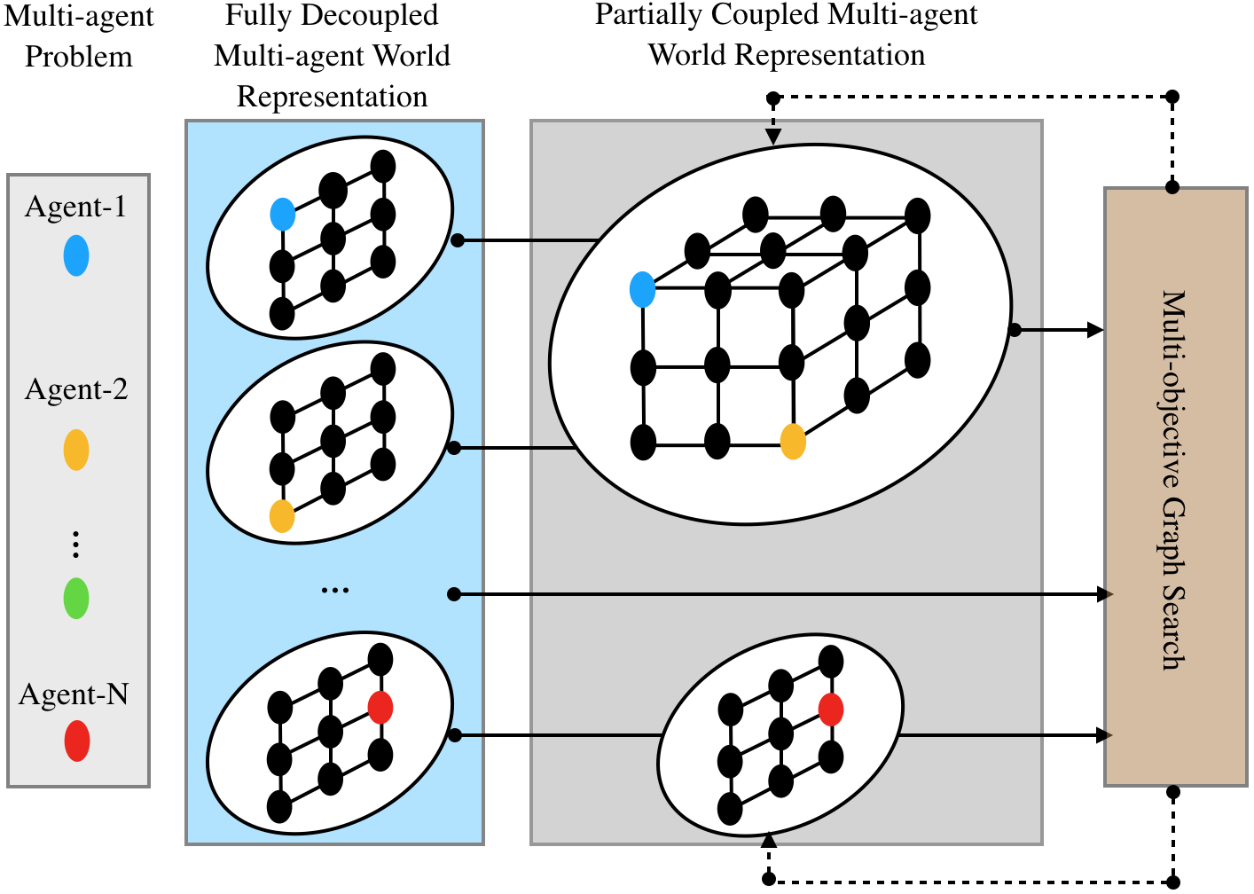
Figure 1: A conceptual illustration of MOM^∗. Agents initially plan their paths independently and are coupled together only when needed. The entire search process optimizes multiple objectives and yields all Pareto-optimal solutions.

In the presence of multiple objectives, in general, there may not be a single optimal solution that optimizes all the objectives. Therefore, we seek a set of Pareto-optimal solutions for multi-objective problems [3]. A solution is Pareto-optimal if there exists no other solution that will yield an improvement in one objective without causing a deterioration in at least one of the other objectives. Finding a Pareto-optimal set for MOMAPF while ensuring conflict-free paths for agents in each solution is quite challenging [17, 33] as the size of the Pareto-optimal set may grow exponentially with respect to the number of agents as well as the dimension of the search space. Even though there are multi-objective single-agent search algorithms, such as NAMOA^∗ [12] and others [23, 16], simply applying them to the joint configuration space of all agents may be inefficient. In this article, we present a new approach called multi-objective M^∗ (MOM^∗) that is complete and aims to find the set of all Pareto-optimal solutions for MOMAPF. This work leverages our subdimensional expansion framework for single-objective MAPF [27], and existing multi-objective dominance techniques [3].

Specifically, MOM^∗ (Fig. 1) begins by letting agents follow their individual “optimal” policies subject to multiple objectives. When an agent-agent conflict is found, MOM^∗ couples those agents together in the same manner as M* [27], which locally increases the dimensionality of the search space and enables MOM^∗ to plan a path in the joint space to resolve conflicts. To compare two paths subject to multiple objectives, MOM^∗ leverages the dominance rules [3]. As a result, MOM^∗ plans in a relatively compact space to find all Pareto-optimal solutions and saves computational effort with respect to the existing graph search approaches such as NAMOA^∗ [12], which plans in the joint space of agents. Additionally, with inflated heuristics [13], MOM^∗ can be modified to a bounded sub-optimal algorithm that trades off between computational efficiency and approximation quality.

To evaluate MOM^∗, we ran tests in various grid-like maps from [22]. As a baseline, we apply NAMOA^∗, a well-known graph search algorithm that computes the exact Pareto-optimal set to the joint graph of all agents to solve MOMAPF. We also compared MOM^∗ with another work from us, namely the multi-objective conflict-based search (MO-CBS) [14], which extends conflict-based search to compute the exact Pareto-optimal set for MOMAPF. We compared all three algorithms under multiple metrics, as functions of both number of agents (as conventional MAPF research does) as well as number of objectives. Our results show that MOM^∗ outperforms NAMOA^∗ in terms of (1) success rates of finding all Pareto-optimal solutions, (2) number of state expanded and (3) run time over various test instances. Comparing with MO-CBS, MOM^∗ achieves better success rates and shorter run time in some maps. There is no leading algorithm over all instances for MOMAPF, which is similar to the observation in the single-objective MAPF [4]. In addition, we also corroborated the inflated MOM^∗, an algorithm which finds sub-optimal solutions, with different heuristic inflation rates under various grids with up to twenty agents. Inflated MOM^∗ demonstrates obviously better scalability than both MOM^∗ and MO-CBS.

The rest of the article is organized as follows. Sec. II reviews the related work and Sec. III defines the MOMAPF problem. MOM^∗ algorithm is described in Sec. IV and its properties are proved in Sec. V. Numerical results are presented in Sec. VI with conclusions in Sec. VII.

II Related Work

II-A Multi-agent Path Finding

MAPF methods tend to fall on a spectrum from centralized to decentralized, trading off completeness and optimality for scalability. On the decentralized side of the spectrum, prioritized approaches [19, 11] achieve scalability by decomposing the joint configuration space into a sequence of individual configuration spaces and plan for agents one after another in a pre-defined sequence, which is not guaranteed to be complete. In the middle of the spectrum, rule-based approaches [10, 30], seek to overcome the curse of dimensionality by resolving agent-agent conflicts with pre-defined primitives. While the approaches compute scalable solutions, they lack completeness and optimality. Unfortunately, these approaches are not complete and often form paths with undesired features. Reduction-based methods transform MAPF to known problems like network flow [33], SAT [24], etc, and rely on the corresponding solvers. Conflict-based search (CBS) [18] is a two level search algorithm that finds optimal paths for agents and has been improved in many ways [1, 8]. Finally, on the centralized side of the spectrum, A^∗-based approaches [21, 5] leverages A^∗-like search and plan in the joint configuration space of all the agents.

Subdimensional expansion [27], as another method stands in the middle of the spectrum, bypasses the curse of dimensionality by dynamically modifying the dimension of the search space based on agent-agent conflicts. This approach applies to many algorithms [29, 28], and inherits completeness and optimality, if the underlying algorithm already has these features. Combining subdimensional expansion with A^∗ results in M^∗ [27]. M^∗ begins by computing a set of individual policies for agents and lets every agent follow its policy towards its goal, initially ignoring agent-agent conflicts. When a conflict is detected, the subset of agents in conflict are locally coupled together to form a new search space with increased dimensions, where a new search is conducted to resolve the conflict. In this work, we combines subdimensional expansion with multi-objective search.

II-B Multi-objective Search

Multi-objective optimization (MOO) has been applied to single-agent path planning [23, 12, 26], motion planning [25], reinforcement learning [15], etc. With respect to MOO for multiple agents, the only known work (we are aware of) is on evolutionary algorithms [31] for a related variant of MOMAPF. Specifically, in [31], the authors consider a variant of MOMAPF where conflicts between the agent’s paths is modeled in one of the objectives and not as a constraint; as a result, a solution in the Pareto-optimal set may have agent’s paths that conflict with each other. In addition, the work in [31] assumes no wait times for agents at any vertex in the graph which greatly reduces the size of the Pareto-optimal set. In this work, we allow for agents to wait at any vertex in the graph and seek conflict-free paths for agents in any feasible solution as in the standard MAPF.

Our approach is closely related to conventional multi-objective (graph) search problems [9], which requires finding all Pareto-optimal paths connecting start and goal vertices within a given graph subject to multi-objectives. One of the basic challenges in multi-objective search is to compute the exact Pareto-optimal set, the size of which can grow exponentially with respect to the number of nodes in a graph [17]. To overcome the challenge, algorithms like A^∗ [6], as a best-first search method, are extended to multi-objective A^∗ (MOA^∗) [23] and later improved by A New Approach to MOA^∗ (NAMOA^∗) [12]. Even though MOA^∗-type algorithms can be applied to the product of the configuration spaces of the agents, numerical results in Sec. VI show that it is significantly less efficient compared to the proposed MOM^∗, which is an algorithm that benefits from the techniques in both MAPF communities and multi-objective search communities.

In parallel with this work, we are also working on multi-objective conflict-based search (MO-CBS) [14], which extends the popular conflict-based search algorithm to compute the exact Pareto-optimal set for MOMAPF. Our results show that there is no leading algorithm in all maps. Additionally, the approximation algorithm proposed in this work, inflated MOM^∗, achieves better scalability than both MOM^∗ and MO-CBS while providing approximated Pareto-optimal set with bound guarantees.

III Problem Definition

Let index set $I=\{1,2,\dots,N\}$ denote a set of $N$ agents. All agents move in a workspace represented as a graph $G=(V,E)$, where the vertex set $V$ represents all possible locations of agents and the edge set $E=V\times V$ denotes the set of all possible actions that move an agent between any two vertices in $V$. An edge between two vertices $u,v\in V$ is denoted as $(u,v)\in E$ and the cost of an edge $e\in E$ is an $M$-dimensional strictly positive real vector: $\text{cost}(e)\in(\mathbb{R}^{+})^{M}\backslash\{0\}$, with $M$ being a positive integer.

In this work, we use a superscript $i\in I$ over a variable to represent the specific agent to which the variable belongs. For example, $v^{i}\in V$ means a vertex with respect to agent $i$. Let $\pi^{i}(v^{i}_{1},v^{i}_{\ell})$ be a path that connects vertices $v^{i}_{1}$ and $v^{i}_{\ell}$ via a sequence of vertices $(v^{i}_{1},v^{i}_{{2}},\dots,v^{i}_{\ell})$ in $G$. Let $g^{i}(\pi^{i}(v^{i}_{1},v^{i}_{\ell}))$ denote the $M$-dimensional cost vector associated with the path, which is the sum of the cost vectors of all the edges present in the path, i.e. $\displaystyle g^{i}(\pi^{i}(v^{i}_{1},v^{i}_{\ell}))=\Sigma_{j=1,2,\dots,{\ell-1}}\text{cost}(v^{i}_{{j}},v^{i}_{{j+1}})$.

All agents share a global clock. Each action, either wait or move, for any agent requires one unit of time. All the agents start their paths at time $t=0$. Any two agents $i,j\in I$ are said to be in conflict if one of the following two cases happens. The first case is a “vertex conflict” where two agents occupy the same vertex at the same time. The second case is an “edge conflict” (also called swap conflict) where two agents move through the same edge from opposite directions between times $t$ and $t+1$ for some $t$.

Let $v_{o}^{i},v^{i}_{f}\in V$ respectively denote the initial location and the final destination of agent $i$. Without loss of generality, to simplify the notations, we also refer to a path $\pi^{i}(v^{i}_{o},v^{i}_{f})$ for agent $i$ between its initial and final locations as simply $\pi^{i}$. Let $\pi=(\pi^{1},\pi^{2},\dots,\pi^{N})$ represent a joint path for all the agents. The cost vector of this joint path is defined as the vector sum of the individual path costs over all the agents, $i.e.$, $g(\pi)=\Sigma_{i}g^{i}(\pi^{i})$. To compare any two joint paths, we compare the cost vectors corresponding to them. Given two vectors $a$ and $b$, $a$ dominates $b$ if every component in $a$ is no larger than the corresponding component in $b$ and there exists at least one component in $a$ that is strictly less than the corresponding component in $b$. Formally, it is defined as follows:

Definition 1 (Dominance [12])

Given two $M$-dimensional vectors $a$ and $b$, $a$ dominates $b$, symbolically $a\succeq b$, if $\forall m\in\{1,2,\dots,M\}$, $a(m)\leq b(m)$, and there exists $m\in\{1,2,\dots,M\}$ such that $a(m)<b(m)$.

If $a$ does not dominate $b$, we represent this non-dominance as $a\nsucceq b$. Any two solution joint paths are non-dominated if the corresponding cost vectors do not dominate each other. The set of all non-dominated solutions is called the Pareto-optimal set. MOMAPF problem aims to find an maximal subset of the Pareto-optimal set, where any two solutions in this subset do not have the same cost vector.

IV Multi-Objective M*

IV-A Notation

Let $\mathcal{G}=(\mathcal{V},\mathcal{E})=\underbrace{G\times G\times\dots\times G}_{\text{$N$ times}}$ denote the joint graph which is the Cartesian product of $N$ copies of graph $G$, where each vertex $v\in\mathcal{V}$ represents a joint vertex and $e\in\mathcal{E}$ represents a joint edge that connects a pair of joint vertices. The joint vertex corresponding to the initial locations of the agents is $v_{o}=(v^{1}_{o},v^{2}_{o},\cdots,v^{N}_{o})$. In addition, let $\pi(u,v),u,v\in\mathcal{V}$ represent a joint path, which is a tuple of $N$ individual paths, $i.e.$, $\pi(u,v)=(\pi^{1}(u^{1},v^{1}),\cdots,\pi^{N}(u^{N},v^{N}))$.

The state of the agents is denoted as $s=(v,g)$, which represents a partial solution: $v$ represents the joint vertex occupied by the agents and $g$ denotes the cost vector of a joint path connecting $v_{o}$ and $v$. For the rest of the work, let $v(s)$ denote the joint vertex in state $s$ and $g(s)$ denote the cost vector. Similarly, let $v^{i}(s)$ denote the individual vertex in $v(s)$ corresponding to agent $i\in I$. Besides, we say a state $s_{k}$ visits joint vertex $v_{l}$ if $v(s_{k})=v_{l}$.

Similar to the A^∗ algorithm, a heuristic (cost) vector is associated with each joint vertex. The heuristic vector of $v\in\mathcal{V}$ is denoted as $h(v)$, which is the sum of the (individual) heuristic vectors of every individual vertex $v^{i}\in v$, $i.e.$ $h(v)=\Sigma_{i\in I}h(v^{i})$ and $h(v^{i})$ is an component-wise underestimate of the cost vectors of all Pareto-optimal paths from $v^{i}$ to $v^{i}_{f}$. Also, the $f$-vector associated with a state $s$ is defined as $f(s):=g(s)+w\cdot h(v(s))$, where $w$ is the heuristic inflation rate with value no less than one.

Let “collision set” $I_{C}(s)\subseteq I$ represent a set of agents in conflict at state $s$. To detect conflicts, collision function $\Psi:\mathcal{V}\times\mathcal{V}\rightarrow 2^{I}$ is introduced to check if there is any vertex or edge conflicts given two adjacent joint vertices. Collision function $\Psi$ returns either an empty set if no conflict is detected, or a set of agents that are in conflict.

As in the well-known A^∗ algorithm [6], at any stage of the algorithm, let OPEN be the open list which contains candidate states to be expanded and let CLOSED represent the set of states that have already been expanded. In addition, states in the OPEN and CLOSED list are organized based on their joint vertices: given a joint vertex $v$, let OPEN($v$) and CLOSED($v$) denote the subset of open and closed states that share the same $v$.

IV-B Algorithm Overview

The proposed MOM^∗ algorithm avoids directly search over the joint graph. Intuitively, MOM^∗ gains computation efficiency by (1) only considering the joint graph of a subset of agents when the agents have to interact to avoid conflicts, and (2) frequently pruning the partial solutions that are dominated.

The pseudo code of MOM^∗ is shown in Algorithm 1. For initialization, the initial state $s_{o}=(v_{o},0)$, where $0$ denotes a zero vector, is added to OPEN. In each iteration of the search loop (from line 4), a state $s_{k}$ with a non-dominated $f$-vector is popped from OPEN. Next, the joint vertex $v(s_{k})$ is compared with the final joint vertex $v_{f}$.

• If $v(s_{k})=v_{f}$, a non-dominated solution can be obtained (line 6) by iteratively back-tracking the parent of each state from $s_{k}$ to $s_{o}$. In addition, the $f$-vector of this non-dominated solution $f(s_{k})$ is used to “filter” all the candidate states in OPEN by calling a sub-procedure (Sec. IV-D5), which prunes any candidate states with $f$-vectors dominated by $f(s_{k})$ (note that $h(v_{k})=h(v_{f})=0$ and $f(s_{k})=g(s_{k})$).

• If $v(s_{k})\neq v_{f}$, state $s_{k}$ (from line 10) is expanded by considering only a limited set of neighbor states $S^{ngh}$ of $s_{k}$ (Sec. IV-D3), which avoids searching over the joint graph directly and reduces the branching factor during the search. The $S^{ngh}$ of $s_{k}$ is controlled by the collision set $I_{C}(s_{k})$. For each neighbor $s_{l}\in S^{ngh}$, collision function $\Psi(v(s_{k}),v(s_{l}))$ is called and the resulting collision set is back-propagated (Sec. IV-D3). This back-propagation updates the collision set of the ancestor states if needed and inserts those ancestor states into OPEN for re-expansion with a larger limited neighbor set. Then, state $s_{l}$ is compared with any other state $s^{\prime}$ that visits $v(s_{l})$ ($i.e.$ $v(s^{\prime})=v(s_{l})$). If cost vector $g(s_{l})$ is dominated by or equal to $g(s^{\prime})$, $s_{l}$ is pruned and a sub-procedure is called to handle collision set back-propagation when dominance happens (Sec. IV-D4). Otherwise, $s_{l}$ is inserted into OPEN as a candidate state for future expansion.

When OPEN becomes empty, there is no candidate state with a non-dominated $f$-vector. The algorithm then terminates and returns $\mathcal{S}$, which is a set that contains all cost-unique non-dominated solutions for MOMAPF.

Algorithm 1 Pseudocode for MOM^∗

1:initialize OPEN and OPEN($v_{o}$) with $s_{o}=(v_{o},{0})$

2:$\mathcal{S}$ $\leftarrow\emptyset$ $\triangleright$ A set of solutions

3:while OPEN not empty do $\triangleright$ Main search loop

4:    $s_{k}\leftarrow$ OPEN.pop()

5:    move $s_{k}$ from OPEN($v(s_{k})$) to CLOSED($v(s_{k})$)

6:    if $v(s_{k})=v_{f}$ then

7:    $\pi\leftarrow$ Reconstruct($s_{k}$) $\triangleright$ Reconstruct joint path

8:    add $\pi$ to $\mathcal{S}$

9:    FilterOpen($s_{k}$) $\triangleright$ Use $s_{k}$ to filter open list

10:    $S^{ngh}\leftarrow$ GetNeighbor($s_{k}$)

11:    for all $s_{l}\in S^{ngh}$  do

12:         $I_{C}(s_{l})\leftarrow I_{C}(s_{l})\bigcup\Psi(v(s_{k}),v(s_{l}))$

13:         BackProp($s_{k}$, $I_{C}(s_{l})$)

14:         $f(s_{l})\leftarrow g(s_{l})$ + $w\cdot h(v_{l})$

15:         if $\Psi(v(s_{k}),v(s_{l}))\neq\emptyset$

16:         continue

17:         if Compare($s_{l}$) then

18:         add $s_{l}$ to OPEN and OPEN($v(s_{l})$)

19:         add $s_{k}$ to back_set($s_{l}$)

20:         parent($s_{l}$) $\leftarrow s_{k}$

21:         else $\triangleright$ Back-propagation due to dominance

22:         DomBackProp($s_{k},s_{l}$)     

23:return $\mathcal{S}$

IV-C Relationship to M^∗

The MOMAPF problem, as defined in Sec. III generalizes the conventional (single-objective) MAPF: when $M=1$, the MOMAPF problem becomes a conventional (single-objective) MAPF problem and the solution set consists of only one solution with the optimal cost value. Similarly, the proposed MOM^∗ algorithm can also be regarded as a generalization of M^∗ to handle multiple objectives. Specifically, when $M=1$, MOM^∗ solves (single-objective) MAPF in the following sense.

• State comparison becomes “$\leq$” (no larger than) relationship between two scalar cost values.

• In every search iteration, a state with a non-dominated ($i.e.$ minimum) cost value in OPEN is popped, which guarantees that the first solution identified is the one with the minimum cost value (denoted as $C^{*}$).

• All candidate states in OPEN have cost no less than $C^{*}$ and are thus pruned in the sub-procedure that filters OPEN with $C^{*}$, which leads to the termination of the algorithm as OPEN becomes empty.

• Procedure DomBackProp and maintaining a set OPEN($v$)$\bigcup$CLOSED($v$) at each joint vertex $v\in\mathcal{V}$ are redundant when $M=1$ since there is only one optimal path from $v_{o}$ to any $v\in\mathcal{V}$ (up to tie).

IV-D Key Parts of Our Approach

IV-D1 State Space

MOM^∗ defines its search state to be a tuple $(v,g)$ consisting of a joint vertex $v$ and a cost vector $g$, which identifies a partial solution from $v_{o}$ to $v$ with cost vector $g$. The reason for such a state definition is rooted at the key difference between single-objective and multi-objective search problems: while there is one optimal path from $v_{o}$ to any $v$ in single-objective settings, there are multiple non-dominated paths $\pi(v_{o},v)$ for any $v\in\mathcal{V}$ for multi-objectives. This state definition allows the algorithm to differentiate between paths $\pi(v_{o},v)$ with different cost vectors.

IV-D2 Pareto Policy

In multi-objective settings, for every agent $i\in I$, there exists multiple non-dominated paths from $v^{i}_{o}$ to a vertex $v^{i}\in V$ and there are also multiple non-dominated paths $\pi^{i}(v^{i},v^{i}_{f})$. Therefore, the optimal policy $\phi^{i}(v^{i})$ maps $v^{i}$ to multiple neighbor vertices, each of which is along some non-dominated path $\pi^{i}(v^{i},v^{i}_{f})$. This differs from the concept of the optimal policy used in M^∗, where $\phi^{i}(v^{i})$ maps $v^{i}$ to only one neighbor along an optimal path from $v^{i}$ to $v^{i}_{f}$. To differentiate, we use term Pareto policy to describe an individual policy $\phi^{i}$ in multi-objective settings for the rest of the article. To compute $\phi^{i},\forall i\in I$, MOM^∗ runs single-agent multi-objective search [12] backwards from $v^{i}_{f}$ to all vertices in $G$.

IV-D3 Limited Neighbors

Limited neighbors is a concept originally introduced in M^∗ and generalized here (by combining Pareto policies) for MOM^∗. The limited neighbors $S^{ngh}_{k}$ of $s_{k}$ is a set of neighbor states that can be reached from $s_{k}$. For each agent $i$, if $i\notin I_{C}(s_{k})$, agent $i$ is only allowed to follow its Pareto policy $\phi^{i}(v^{i}_{k})$. If $i\in I_{C}(s_{k})$, agent $i$ is allowed to visit any neighbor of $v^{i}_{k}$ in $G$. Formally,

$$S^{ngh}_{k}=\{s_{l}\bigg{|}\begin{cases}v^{i}(s_{l})\in\phi^{i}(v^{i}(s_{k}))&\mbox{if }i\notin I_{C}(s_{k})\\ v^{i}(s_{l})|(v^{i}(s_{k}),v^{i}(s_{l}))\in E&\mbox{if }i\in I_{C}(s_{k})\end{cases},$$

$$g(s_{l})=g(s_{k})+\Sigma_{i\in I}(\text{cost}(v^{i}(s_{k}),v^{i}(s_{l})))\;\}.$$ (1)

Limited neighbors of a state $s$ varies once $I_{C}(s_{k})$ changes, which dynamically modifies the sub-graph embedded in joint graph $\mathcal{G}$ that can be reached from $s_{k}$. Collision set $I_{C}(s_{k})$ is updated (enlarged) recursively when Algorithm 2 is called (line 12 in Algorithm 1). To keep track of the states that should be back-propagated to, a data structure “back_set” is defined at every search state. Intuitively, the back_set at state $s_{k}$ contains all parent states from which $s_{k}$ is ever reached. When $I_{C}(s_{k})$ is enlarged, $I_{C}(s_{k})$ is back-propagated to every state in back_set($s_{k}$).

Algorithm 2 Pseudocode for BackProp

1:INPUT: $s_{k}$, $I_{C}(s_{l})$

2:if $I_{C}(s_{l})\nsubseteq I_{C}(s_{k})$ then

3:$I_{C}(s_{k})\leftarrow I_{C}(s_{l})\bigcup I_{C}(s_{k})$

4:if $s_{k}\notin$ OPEN then

5:add $s_{k}$ to OPEN and OPEN($v(s_{k})$)

6:remove $s_{k}$ from CLOSED($v(s_{k})$)

7:for all $s_{k}^{\prime}\in$ back_set($s_{k}$) do

8:BackProp($s_{k}^{\prime}$, $I_{C}(s_{k})$)

When back-propagating a collision set $I_{C}(s_{l})$ to a state $s_{k}\in$ back_set($s_{l}$), if $I_{C}(s_{k})$ is not a super set of $I_{C}(s_{l})$, then $I_{C}(s_{k})$ is updated by taking the union of $I_{C}(s_{l})$ (line 3). In addition, $s_{k}$ is re-inserted into OPEN (and OPEN($v(s_{k})$)) from CLOSE (and CLOSE($v(s_{k})$)), which makes MOM^∗ expand $s_{k}$ again with a possibly larger limited neighbor set.

IV-D4 State Comparison

Given a joint vertex $v\in\mathcal{V}$, let $\alpha(v),v\in\mathcal{V}$ denote the “frontier set at $v$”: a subset of states that visits $v$ with non-dominated cost vectors. In MOM^∗, set OPEN($v$)$\bigcup$CLOSE($v$) forms a super set of $\alpha(v)$. When MOM^∗ expands $s_{k}$ and generates state $s_{l}$, to decide whether $s_{l}$ should be pruned or not (line 17 in Algorithm 1), $g(s_{l})$ is compared with the cost vector $g(s^{\prime}),\forall s^{\prime}\in$ OPEN($v(s_{l})$)$\bigcup$CLOSE($v(s_{l})$).

• If $g(s_{l})$ is dominated by (or equal to) $g(s^{\prime})$, $s_{l}$ can not be part of $\alpha(v)$ and is thus pruned. In addition, MOM^∗ back-propagates the collision set at $s^{\prime}$ to $s_{k}$ and then add $s_{k}$ to the back_set($s^{\prime}$) before discarding $s_{l}$. By doing so, MOM^∗ keeps updating collision sets of any ancestor states of $s_{l}$ after $s_{l}$ is pruned.

• Otherwise, $s_{l}$ may represent a non-dominated partial solution from $v_{o}$ to $v$ and is therefore inserted into OPEN and OPEN($v(s_{l})$) and becomes part of set OPEN($v(s_{l})$)$\bigcup$CLOSE($v(s_{l})$) permanently.

Algorithm 3 Pseudocode for DomBackProp

1:INPUT: $s_{k},s_{l}$ $\triangleright$ $s_{l}$ is generated from $s_{k}$

2:for all $s^{\prime}$ in OPEN($v(s_{l})$)$\bigcup$CLOSED($v(s_{l})$) do

3:if $g(s^{\prime})\succeq g(s_{l})\text{ or }g(s^{\prime})=g(s_{l})$ then

4:BackProp($s_{k}$, $I_{C}(s^{\prime})$)

5:add $s_{k}$ to back_set($s^{\prime}$)

IV-D5 Termination Condition and Heuristic Inflation

Different from M^∗, which terminates when the first solution is identified, MOM^∗ terminates only when OPEN is empty, to identify all Pareto-optimal solutions. For a MOMAPF problem, however, OPEN is often prohibitively huge since the joint vertex space grows exponentially with respect to the number of agents. To avoid unnecessary state expansion, multi-objective search algorithms often use the cost vector of a state $s_{k}$ that visits $v_{f}$ to filter candidates states in OPEN and prune those with dominated cost vectors. In this work, when $v(s_{k})=v_{f}$, we compare the $f$-vectors of both $s_{k}$ and the candidate states in OPEN. States in OPEN with dominated $f$-vectors are filtered. As the heuristic vector is an component-wise underestimate of the cost-to-goal, when $w=1$, MOM^∗ algorithm does not prune any candidate states that are part of a non-dominated solution.

The use of $f$-vectors in the filtering procedure allows MOM^∗ to utilize inflated heuristics to trade off between search efficiency and bounded sub-optimality, as commonly done in A^∗ [13] or M^∗-based algorithms [27]. For MOM^∗, when $w>1$, it is guaranteed that for any Pareto-optimal solution with cost vector $g^{*}$, inflated MOM^∗ is able to find a sub-optimal solution with cost vector $g$ that’s in the “proximity” of $g^{*}$ and such proximity is bounded by $w$. Detailed proof is provided in Sec. V.

Algorithm 4 Pseudocode for FilterOpen

1:INPUT: $s_{k}$ $\triangleright$ $v(s_{k})=v_{f}$

2:for all $s_{l}$ in OPEN do

3:if$f(s_{k})\succeq f(s_{l})\text{ or }f(s_{k})=f(s_{l})$ then

4:move $s_{l}$ from OPEN($v(s_{l})$) to CLOSED($v(s_{l})$)

5:remove $s_{l}$ from OPEN

V Theoretical Properties of MOM*

Theorem 1 (Completeness and optimality)

If there is no solution, MOM^∗ terminates in finite time and reports failure; otherwise, MOM^∗ finds all cost-unique Pareto-optimal joint paths connecting $v_{o}$ and $v_{f}$.

Proof:

We provide a sketch proof to concisely highlight the overall flow and key steps. Let $\Pi_{*}$ denote a set of all cost-unique conflict-free Pareto-optimal joint paths connecting $v_{o}$ and $v_{f}$ in $\mathcal{G}$. Let $\mathcal{G}^{sch}$ represent the search graph: the sub-graph of $\mathcal{G}$ that is reachable from $v_{o}$ by iteratively following limited neighbors. By the construction of MOM^∗ algorithm (Alg. 1), during the search process, MOM^∗ either grows $\mathcal{G}^{sch}$ by modifying collision set at search states or conducts A^∗-like search in $\mathcal{G}^{sch}$ by selecting a candidate state with non-dominated cost vector for expansion from OPEN.

We first claim that (claim 1) MOM^∗ can identify all cost-unique Pareto-optimal solutions within $\mathcal{G}^{sch}$ because MOM^∗ expands a state by generating all possible neighbors of that state in $\mathcal{G}^{sch}$ and terminates only when OPEN is empty. Thus, if $\mathcal{G}^{sch}$ contains all $\pi_{*}\in\Pi_{*}$, MOM^∗ can find all of them. Next, we claim that If there exists a $\pi_{*}\in\Pi_{*}$ that is not contained in $\mathcal{G}^{sch}$, then there must exist a corresponding joint path $\pi^{\prime}$ such that (1) there is a conflict along $\pi^{\prime}$ and (2) $g(\pi_{*})\nsucceq g(\pi^{\prime})$. Here, condition (2) guarantees that states along $\pi^{\prime}$ will by expanded by MOM^∗ before termination and condition (1) guarantees that a conflict will be identified during the state expansion, which grows $\mathcal{G}^{sch}$ and eventually includes $\pi^{*}$ into $\mathcal{G}^{sch}$. Therefore, combining with the previous claim (claim 1), MOM^∗ computes all cost-unique Pareto-optimal solutions in $\Pi_{*}$.

If there is no feasible joint path from $v_{o}$ to $v_{f}$ in $\mathcal{G}$, MOM^∗ modifies $\mathcal{G}^{sch}$ for a finite number of times because $\mathcal{G}$ is finite and there is only a finite number of partial solutions from $v_{o}$ to any other joint vertices in $\mathcal{G}$. This guarantees that MOM^∗ terminates in finite time without returning a solution. ∎

Theorem 2 (Bounded sub-optimality)

When a heuristic is inflated by a factor of $w>1$, for any Pareto-optimal path $\pi^{*}$ with non-dominated cost vector $g^{*}$, within $\mathcal{S}$ returned by MOM^∗, there exists a joint path $\pi$ with cost vector $g$ such that $g(m)<w\cdot g^{*}(m),m=1,2,\dots,M$.

Proof:

Let $s$ be a state expanded by MOM^∗ with $v(s)=v_{f}$ and let $s^{\prime}$ be a state that is filtered from OPEN when compared with $s$ in Algorithm 4. Let $h^{*}(v(s^{\prime}))$ be the true cost vector of an arbitrary Pareto-optimal path from $v(s^{\prime})$ to $v_{f}$ and let $f^{*}(s^{\prime})=g(s^{\prime})+h^{*}(v(s^{\prime}))$.

As $h(v(s^{\prime}))$ component-wise underestimates $h^{*}(v(s^{\prime}))$, $w\cdot f^{*}(s^{\prime})\geq w(g(s^{\prime})+h(v(s^{\prime})))$. Since $w>1$, $w(g(s^{\prime})+h(v(s^{\prime})))>f(s^{\prime})=g(s^{\prime})+wh(v(s^{\prime}))$. Since $s^{\prime}$ is filtered from OPEN when compared with $s$, $f(s^{\prime})=g(s^{\prime})+wh(v(s^{\prime}))>f(s)=g(s)+wh(v(s))$. As $v(s)=v_{f}$, it means $h(v(s))=0$ and $f(s)=g(s)+wh(v(s))=g(s)$. Put them together, we have $wf^{*}(s^{\prime})>g(s)$. If the filtered state $s^{\prime}$ is part of a Pareto-optimal path (with Pareto-optimal cost vector $f^{*}(s^{\prime})$), then MOM^∗ finds a solution with cost vector $g(s)<wf^{*}(s^{\prime})$. ∎

VI Numerical Results

We implemented both MOM^∗ and NAMOA^∗ [12] in Python. The NAMOA^∗ is applied to the the joint graph $\mathcal{G}$ of agents and serves as a baseline approach. As we are working on extending conflict-based search [18] to multi-objective conflict-based search (MO-CBS) [14], the preliminary results of a Python implementation of MO-CBS is also reported here for comparison. All algorithms are tested on a computer with a CPU of Intel Core i7 and 16GB RAM. To test the algorithms, we selected four maps (grids) from different categories [22] and generate an un-directed graph $G$ by making each grid four-connected. To assign cost vectors to edges, we first assign every agent a cost vector $a^{i}$ of length $M$ (the number of objectives) for all agents $i$, and assign every edge $e$ in graph $G$ a scaling vector $b(e)$ of length $M$, where each component in both $a^{i}$ and $b(e)$ are randomly sampled from integers in $[1,10]$. The cost vector for agent $i$ to go through an edge $e$ is the component-wise product of $a^{i}$ and $b(e)$. If agent $i$ waits in place, the cost vector incurred is $a^{i}$. We tested the algorithms with different heuristic inflation rates $w$, different number of objectives $M$ and different number of agents $N$. We limited the computation time of each instance to five minutes.

VI-A Implementation of heuristics and Pareto policies

In our implementation, to compute heuristics $h(v),v\in\mathcal{V}$, we first run single-agent NAMOA^∗ search backwards from $v^{i}_{f}$ to all other vertices in $G$ for all agents $i\in I$, which computes the set of all Pareto-optimal cost vectors $\{g^{i}_{*}\}$ of paths $\pi^{i}(v^{i}_{f},u)$ that connects $v^{i}_{f}$ with $u\in V$ for all $i\in I$. Then, for each (individual) vertex $u$ in $G$, the component-wise minimum over all vectors in $\{g^{i}_{*}\}$ forms a cost vector $h^{i}(u)$ which underestimates the cost vectors of any path from $u$ to $v^{i}_{f}$. Finally, the heuristic value of a joint vertex $v\in\mathcal{V}$ is computed by $h(v)=\Sigma_{i\in I}h^{i}(v^{i})$, where $v^{i}$ is the individual vertex contained in $v$ for agent $i$. As this computation finds the individual Pareto-optimal paths at each node for each agent, the Pareto policy for each agent is also constructed. The heuristics are computed before the search begins for both NAMOA^∗ and MOM^∗, and the computation time is included in the run time we report next.

VI-B Experiments with Different Numbers of Objectives

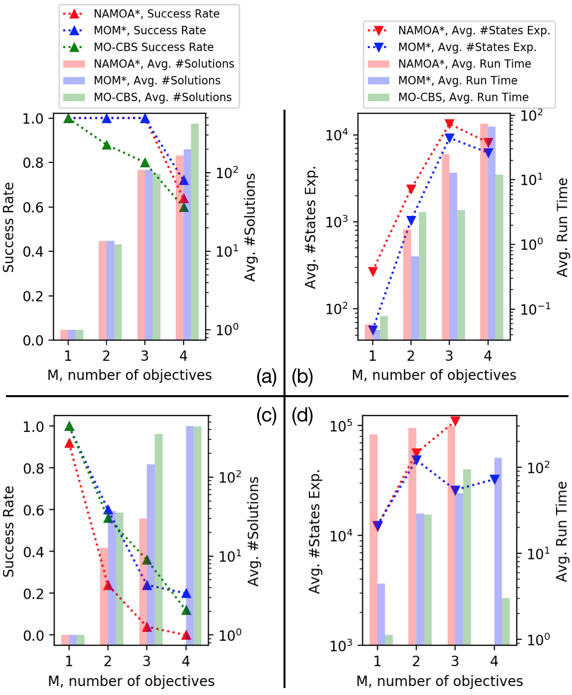
Figure 2: Comparing MOM^∗, NAMOA^∗ and MO-CBS with a fixed number of agents $N$ and varying number of objectives $M$. In plots (a) and (b), $N=2$. In plots (c) and (d), $N=4$.

We begin our tests with the a free grid of size 16 by 16 (“empty-16-16”) and the result is shown in Fig. 2. When $N=2$, from (a), both NAMOA^∗ and MOM^∗ computes all Pareto-optimal solutions for almost all the instances and outperforms MO-CBS. The average number of Pareto-optimal solutions grows from one to $\approx$ one hundred when $M$ grows from one to three. This trend indicates the difficulty of the problems with an increasing $M$: for the same graph with a fixed $N$, problems with a larger $M$ typically have more Pareto-optimal solutions and can take longer time for all three algorithms to compute. Notice that when $M=1$, the MOMAPF problem becomes the conventional (single-objective) MAPF problem where an optimal solution is computed. From (b), we observe a similar increase in both the average number of states expanded and run time over solved instances. However, MOM^∗ expands fewer states and runs faster than NAMOA^∗ on average.

When $N=4$, from (c), MOM^∗ performs better than NAMOA^∗ and similar to MO-CBS in terms of success rates. Since MOM^∗ solves more instances than NAMOA^∗, the results in (d) becomes less informative. But even when MOM^∗ solves more (possibly hard) instances, the run time of MOM^∗ is still obviously shorter than NAMOA^∗.

VI-C Experiments with Different Number of Agents

Fixing $M=2$ (two objectives), we evaluate all three algorithms in different maps in terms of (1) success rates of finding all Pareto-optimal solutions, (2) the average number of states expanded for NAMOA^∗ and MOM^∗, and (3) average number of solutions computed, with a varying number of agents $N$. The averages are taken over solved instances. As shown in Table I, MOM^∗ (without heuristic inflation) outperforms NAMOA^∗ as it achieves higher success rates and expands fewer states (when the success rates are similar). Comparing with MO-CBS, MOM^∗ (without heuristic inflation) performs better than MO-CBS in the room map and worse in “den312d” map. In multi-objective settings, similar to the observation in [4], there is no single multi-agent planner that outperforms all other planners in all maps.

VI-D Inflated MOM^∗ in Different Maps

Map	Alg.	Success rates / Avg. #states expanded (in thousand) / Avg. #solutions found
		N=2	N=4	N=8	N=12	N=16	N=20
	NAMOA∗	1.00/ 3.3/ 11.2	0.16/ 78.1/ 14.3	0/ -/ -	0/ -/ -	0/ -/ -	0/ -/ -
	MO-CBS	0.88/ -/ 11.1	0.48/ -/ 25.0	0.08/ -/ 72.5	0/ -/ -	0/ -/ -	0/ -/ -
	MOM∗	1.00/ 1.4/ 11.2	0.76/ 36.0/ 28.7	0.12/ 65.6/ 59.7	0/ -/ -	0/ -/ -	0/ -/ -
	MOM∗ w=1.1	1.00/ 0.1/ 2.7	0.96/ 1.5/ 1.9	0.76/ 46.1/ 2.4	0.24/ 5.8/ 1.8	0.08/ 140.6/ 1.0	0/ -/ -
	MOM∗ w=1.2	1.00/ 0.06/ 1.5	0.96/ 0.4/ 1.3	0.80/ 5.7/ 1.6	0.48/ 47.0/ 1.4	0.24/ 146.4/ 1.5	0/ -/ -
	MOM∗ w=1.5	1.00/ 0.05/ 1.0	1.00/ 1.2/ 1.0	0.96/ 3.4/ 1.1	0.84/ 21.9/ 1.1	0.56/ 162.7/ 1.1	0.04/ 321.9/ 1.0
(Room, 32x32)	MOM∗ w=2.0	1.00/ 0.05/ 1.0	1.00/ 0.8/ 1.0	1.00/ 8.5/ 1.1	0.96/ 22.4/ 1.1	0.68/ 69.8/ 1.0	0.16/ 56.8/ 1.0
	NAMOA∗	0.96/ 40.6/ 34.9	0/ -/ -	0/ -/ -	0/ -/ -	0/ -/ -	0/ -/ -
	MO-CBS	0.68/ -/ 36.5	0.20/ -/ 128.2	0/ -/ -	0/ -/ -	0/ -/ -	0/ -/ -
	MOM∗	0.96/ 8.3/ 34.9	0.16/ 123.1/ 74.8	0/ -/ -	0/ -/ -	0/ -/ -	0/ -/ -
	MOM∗ w=1.1	1.00/ 0.4/ 4.6	1.00/ 2.0/ 5.0	0.72/ 88.8/ 3.3	0.16/ 136.1/ 2.0	0/ -/ -	0/ -/ -
	MOM∗ w=1.2	1.00/ 0.1/ 1.9	1.00/ 6.8/ 2.1	0.84/ 20.4/ 1.8	0.36/ 112.9/ 1.6	0.08/ 68.3/ 1.0	0/ -/ -
	MOM∗ w=1.5	1.00/ 0.1/ 1.2	1.00/ 0.7/ 1.3	1.00/ 12.4/ 1.2	0.92/ 118.7/ 1.3	0.16/ 106.4/ 1.3	0/ -/ -
(Maze, 32x32)	MOM∗ w=2.0	1.00/ 0.1/ 1.1	1.00/ 0.6/ 1.2	1.00/ 8.5/ 1.0	0.96/ 76.2/ 1.1	0.40/ 78.0/ 1.1	0.04/ 108.0/ 1.0
	NAMOA∗	0.32/ 121/ 57.9	0/ -/ -	0/ -/ -	0/ -/ -	0/ -/ -	0/ -/ -
	MO-CBS	0.72/ -/ 105.7	0.12/ -/ 180.3	0/ -/ -	0/ -/ -	0/ -/ -	0/ -/ -
	MOM∗	0.56/ 52.5/ 88.9	0.04/ 74.6/ 106.0	0/ -/ -	0/ -/ -	0/ -/ -	0/ -/ -
	MOM∗ w=1.1	1.00/ 12.2/ 18.7	0.88/ 18.7/ 9.0	0/ -/ -	0/ -/ -	0/ -/ -	0/ -/ -
	MOM∗ w=1.2	1.00/ 0.6/ 5.6	1.00/ 7.6/ 2.9	0.20/ 12.2/ 3.2	0/ -/ -	0/ -/ -	0/ -/ -
	MOM∗ w=1.5	1.00/ 0.2/ 1.5	1.00/ 0.4/ 1.2	0.24/ 5.5/ 1.2	0/ -/ -	0/ -/ -	0/ -/ -
(den312d, 65x81)	MOM∗ w=2.0	1.00/ 0.2/ 1.2	1.00/ 0.3/ 1.1	0.28/ 5.0/ 1.1	0/ -/ -	0/ -/ -	0/ -/ -

TABLE I: Numerical results in various environments with two objectives ($M=2$).

To investigate the impact of inflated heuristics of MOM^∗ as well as how inflated MOM^∗ approximates Pareto-optimal set, Table I shows the numerical results of MOM^∗ with different inflation rates in different maps.

From Table I, inflated heuristics enable MOM^∗ to improve the computational efficiency by approximating Pareto-optimal sets. First, for the same $N$ (the same column in the table) and similar success rates, as $w$ increases, MOM^∗ expands fewer states and thus terminates earlier. Second, MOM^∗ with larger $w$ finds fewer (bounded sub-optimal) solutions. Finally, MOM^∗ is able to solve more instances with larger $N$ while MOM^∗ with smaller or no heuristic inflation fails.

VI-E Time for Computing Pareto Policies

Finally, we investigate the required effort for the pre-processing step, where heuristics and Pareto policies are computed. Table II shows the computational time needed with $M=1,2,3,4$ in a 16x16 empty map. When $M=1$, Pareto policies for agents becomes the conventional optimal policies for agents as used in M^∗ [27] since there is only one optimal neighbor for agent $i\in I$ to choose at any vertices along its path to its goal. In this case, the efforts for pre-processing is equivalent to an exhaustive backwards A^∗ (or Dijkstra) search over the graph for each agent, which is computationally cheap (0.037 seconds) from our results. However, as $M$ increases, it takes significantly more time to compute Pareto policies since exhaustive multi-objective search over a graph is much more burdensome (114.07 seconds when $M=4$).

Table III shows the required time for pre-processing with two objectives ($M=2$ fixed) in different maps. From the table, the size of the map is a decisive factor. However, maps with the same size but of different types may also have obviously different computing time for Pareto policies, which is worthwhile for further exploration.

M	1	2	3	4
Time (seconds)	0.037	0.46	5.65	114.07

TABLE II: Pre-processing time as a function of $M$ with $N=2$.

Map (Width x Height)	Time (seconds)
Empty (16x16)	0.46
Room (32x32)	0.92
Maze (32x32)	4.99
den312d (65x81)	76.88

TABLE III: Pre-processing time when $M=2$, $N=2$ in different maps.

VII Conclusions and Future Work

A new algorithm called MOM^∗ and its variant inflated MOM^∗ were presented for a multi-objective, multi-agent problem. We prove that MOM^∗ is complete and finds all cost-unique Pareto-optimal solutions. Numerical results were also presented to compare the performance of MOM^∗ with the existing methods.

There are several directions for future work in this area. The current approach considers additive costs across agents and one can extend the method to other types of cost such as makespan. This work considers minimization type of problem and one can explore how to apply the proposed algorithm to maximization type of problem such as multi-objective information gathering [2]. One can also focus on extending other MAPF algorithms from single-objective to multi-objectives such as EPEA^∗ [5], SAT-based methods [24]. Another direction is about approximating the Pareto-optimal set via different approaches other than inflated heuristics, such as ideas from multi-objective evolutionary algorithms.

References

- [1] Eli Boyarski, Ariel Felner, Roni Stern, Guni Sharon, David Tolpin, Oded Betzalel, and Eyal Shimony. Icbs: improved conflict-based search algorithm for multi-agent pathfinding. In Twenty-Fourth International Joint Conference on Artificial Intelligence, 2015.
- [2] Weizhe Chen and Lantao Liu. Pareto monte carlo tree search for multi-objective informative planning. In Robotics: science and systems, 2019.
- [3] Matthias Ehrgott. Multicriteria optimization, volume 491. Springer Science & Business Media, 2005.
- [4] Ariel Felner, Roni Stern, Solomon Eyal Shimony, Eli Boyarski, Meir Goldenberg, Guni Sharon, Nathan Sturtevant, Glenn Wagner, and Pavel Surynek. Search-based optimal solvers for the multi-agent pathfinding problem: Summary and challenges. In Tenth Annual Symposium on Combinatorial Search, 2017.
- [5] Meir Goldenberg, Ariel Felner, Roni Stern, Guni Sharon, Nathan Sturtevant, Robert C Holte, and Jonathan Schaeffer. Enhanced partial expansion a. Journal of Artificial Intelligence Research, 50:141–187, 2014.
- [6] P. E. Hart, N. J. Nilsson, and B. Raphael. A formal basis for the heuristic determination of minimum cost paths. IEEE Transactions on Systems Science and Cybernetics, 4(2):100–107, 1968.
- [7] Samira Hayat, Evşen Yanmaz, Timothy X Brown, and Christian Bettstetter. Multi-objective uav path planning for search and rescue. In 2017 IEEE International Conference on Robotics and Automation (ICRA), pages 5569–5574. IEEE, 2017.
- [8] Jiaoyang Li, Wheeler Ruml, and Sven Koenig. Eecbs: A bounded-suboptimal search for multi-agent path finding. arXiv preprint arXiv:2010.01367, 2020.
- [9] Ronald Prescott Loui. Optimal paths in graphs with stochastic or multidimensional weights. Communications of the ACM, 26(9):670–676, 1983.
- [10] Ryan J Luna and Kostas E Bekris. Push and swap: Fast cooperative path-finding with completeness guarantees. In Twenty-Second International Joint Conference on Artificial Intelligence, 2011.
- [11] Hang Ma, Daniel Harabor, Peter J Stuckey, Jiaoyang Li, and Sven Koenig. Searching with consistent prioritization for multi-agent path finding. In Proceedings of the AAAI Conference on Artificial Intelligence, volume 33, pages 7643–7650, 2019.
- [12] Lawrence Mandow, JL Pérez De la Cruz, et al. A new approach to multiobjective a* search. In IJCAI, volume 8. Citeseer, 2005.
- [13] Judea Pearl. Intelligent search strategies for computer problem solving. Addision Wesley, 1984.
- [14] Zhongqiang Ren, Sivakumar Rathinam, and Howie Choset. Multi-objective conflict-based search for multi-agent path finding. arXiv preprint arXiv:2101.03805, 2021.
- [15] Diederik M Roijers, Peter Vamplew, Shimon Whiteson, and Richard Dazeley. A survey of multi-objective sequential decision-making. Journal of Artificial Intelligence Research, 48:67–113, 2013.
- [16] Antonio Sedeño-Noda and Marcos Colebrook. A biobjective dijkstra algorithm. European Journal of Operational Research, 276(1):106–118, 2019.
- [17] Paolo Serafini. Some considerations about computational complexity for multi objective combinatorial problems. In Recent advances and historical development of vector optimization, pages 222–232. Springer, 1987.
- [18] Guni Sharon, Roni Stern, Ariel Felner, and Nathan R Sturtevant. Conflict-based search for optimal multi-agent pathfinding. Artificial Intelligence, 219:40–66, 2015.
- [19] David Silver. Cooperative pathfinding. pages 117–122, 01 2005.
- [20] Amir R Soltani, Hissam Tawfik, John Yannis Goulermas, and Terrence Fernando. Path planning in construction sites: performance evaluation of the dijkstra, a*, and ga search algorithms. Advanced engineering informatics, 16(4):291–303, 2002.
- [21] Trevor Scott Standley. Finding optimal solutions to cooperative pathfinding problems. In Twenty-Fourth AAAI Conference on Artificial Intelligence, 2010.
- [22] Roni Stern, Nathan Sturtevant, Ariel Felner, Sven Koenig, Hang Ma, Thayne Walker, Jiaoyang Li, Dor Atzmon, Liron Cohen, TK Kumar, et al. Multi-agent pathfinding: Definitions, variants, and benchmarks. arXiv preprint arXiv:1906.08291, 2019.
- [23] Bradley S. Stewart and Chelsea C. White. Multiobjective a*. J. ACM, 38(4):775–814, October 1991.
- [24] Pavel Surynek, Ariel Felner, Roni Stern, and Eli Boyarski. Modifying optimal sat-based approach to multi-agent path-finding problem to suboptimal variants. 07 2017.
- [25] Matthew Tesch, Jeff Schneider, and Howie Choset. Expensive multiobjective optimization for robotics. In 2013 IEEE International Conference on Robotics and Automation, pages 973–980. IEEE, 2013.
- [26] Carlos Hernández Ulloa, William Yeoh, Jorge A Baier, Han Zhang, Luis Suazo, and Sven Koenig. A simple and fast bi-objective search algorithm. In Proceedings of the International Conference on Automated Planning and Scheduling, volume 30, pages 143–151, 2020.
- [27] Glenn Wagner and Howie Choset. Subdimensional expansion for multirobot path planning. Artificial Intelligence, 219:1–24, 2015.
- [28] Glenn Wagner and Howie Choset. Path planning for multiple agents under uncertainty. In Twenty-Seventh International Conference on Automated Planning and Scheduling, 2017.
- [29] Glenn Wagner, Minsu Kang, and Howie Choset. Probabilistic path planning for multiple robots with subdimensional expansion. In 2012 IEEE International Conference on Robotics and Automation, pages 2886–2892. IEEE, 2012.
- [30] Ko-Hsin Cindy Wang, Adi Botea, et al. Fast and memory-efficient multi-agent pathfinding. In ICAPS, pages 380–387, 2008.
- [31] J. Weise, S. Mai, H. Zille, and S. Mostaghim. On the scalable multi-objective multi-agent pathfinding problem. In 2020 IEEE Congress on Evolutionary Computation (CEC), pages 1–8, 2020.
- [32] Peter R Wurman, Raffaello D’Andrea, and Mick Mountz. Coordinating hundreds of cooperative, autonomous vehicles in warehouses. AI magazine, 29(1):9–9, 2008.
- [33] Jingjin Yu and Steven M LaValle. Structure and intractability of optimal multi-robot path planning on graphs. In Twenty-Seventh AAAI Conference on Artificial Intelligence, 2013.