Probabilistic Trust Intervals for Out of Distribution Detection

Abstract

Building neural network classifiers with an ability to distinguish between in and out-of distribution inputs is an important step towards faithful deep learning systems. Some of the successful approaches for this, resort to architectural novelties, such as ensembles, with increased complexities in terms of the number of parameters and training procedures. Whereas some other approaches make use of surrogate samples, which are easy to create and work as proxies for actual out-of-distribution (OOD) samples, to train the networks for OOD detection. In this paper, we propose a very simple approach for enhancing the ability of a pretrained network to detect OOD inputs without even altering the original parameter values. We define a probabilistic trust interval for each weight parameter of the network and optimize its size according to the in-distribution (ID) inputs. It allows the network to sample additional weight values along with the original values at the time of inference and use the observed disagreement among the corresponding outputs for OOD detection. In order to capture the disagreement effectively, we also propose a measure and establish its suitability using empirical evidence. Our approach outperforms the existing state-of-the-art methods on various OOD datasets by considerable margins without using any real or surrogate OOD samples. We also analyze the performance of our approach on adversarial and corrupted inputs such as CIFAR-10-C and demonstrate its ability to clearly distinguish such inputs as well.

1 Introduction

Deep neural network classifiers match the human level accuracy in many applications when test data is sampled from a distribution which is same or approximately similar to the training data distribution, also known as in-distribution (ID) data [19, vgg10, 10, 5, 35]. However, the networks fail in presence of data which comes from a different distribution, known as out-of-distribution (OOD) data [26, 13]. These networks perform classification with an assumption of complete knowledge of the classes and therefore, wrongly classify the OOD inputs into the known categories, often with high confidence [27]. In real world scenarios, it is challenging to ensure the similarity of training and test data distributions [1] which raises concerns on the predictions made by deep neural networks due to their vulnerability against OOD inputs.

A solution to the above problem is to design networks which can detect OOD inputs and hence, produce reliable results. One successful design choice in this direction is to use siblings of a network. These siblings are often the copies of a single network with different weight parameter values. The siblings with similar architecture but different weights are expected to produce different outputs for the same input, therefore, are trained on ID data to produce identical outputs for an ID input. As a result, disagreement between the outputs of siblings for ID inputs reduces and it becomes an indicator of OOD inputs whenever a large value observed. For a robust detection, all the weights among the siblings are varied to explore a diverse functional space, for example in deep ensembles [20, 8]. This naturally increases computational burden in terms of training and testing along with increased memory requirements. A trade-off to limit the memory expenses is to allow only few of the weights to vary among the siblings while assigning equal values to the rest or sharing the rest of the weights [33]. Another alternate to create such siblings is to learn distributions over the weight parameters, motivated from the Bayesian principles. However such networks are computationally more complex and often pose a challenge in terms of convergence for deep architectures [20].

In this paper, we propose a simple approach to create siblings of an already trained network. We define a probabilistic trust interval for each weight around its optimized value. It allows to sample multiple values for each weight parameter and produce corresponding outputs for a single input. The sizes of these intervals are optimized for ID data such that the disagreement among multiple outputs for an ID input is minimized. Fig. 1 shows an illustration of probabilistic trust intervals for some of the randomly picked weights of a standard network where the observed interval sizes before (in red) and after (in green) optimization are presented. Centers of the intervals represent the original optimized values of the corresponding weight parameters. For each parameter, values around the center are sampled with higher probability as compared to the values near to the boundary of the interval. It ensures that accuracy of the considered network on ID inputs is maintained while enabling OOD detection mechanism.

Figure 1: Illustration of Probabilistic Trust Intervals for randomly picked weights of neural classifier before (red) and after (green) training. Trust intervals before training are of same size for each weight and get adjusted to ID data after training for maintaining the generalization abilities of the underlying neural network while enabling OOD detection.

Optimization of the probabilistic trust intervals’ sizes is the most critical component of our proposed approach. These intervals should be small enough to not allow the network siblings to go far off from the optimal point. At the same time, the interval sizes should be large enough to produce distinguishable output variations between ID and OOD data. For this purpose, we design a loss function which tries to optimise the size of intervals around each weight such that inside these intervals the output variations are small for ID inputs. Subsequently, these variations are used to quantify the similarity among the outputs of different sibling networks using a newly designed measure of agreement. The deployment of probabilistic trust intervals around weights with measure of agreement on the trained networks enables OOD detection without using any kind of OOD validation samples or surrogate proxies of OOD data.

We evaluate our method on different shallow and deep neural classifiers, including VGG-16 [30], ResNet-20 [10] and DenseNet-100 [15]. We use MNIST [21], CIFAR-10 [17], SVHN [25], CIFAR-100 [18], Fashion-MNIST [34], CMATERDB [6], and Gaussian images, where each pixel is sampled from $\mathcal{N}(0,1)$. Our approach outperforms previous works related to OOD input detection in most of the experiments. For example, the False Positive Rate at 95% True Positive Rate, for MNIST as ID and Fashion-MNIST as OOD data, is found to be 12.46% by using just 2 sets of weights as compared to 27.48% which is the best among the considered baselines. In addition, we also tested our approach on corrupted CIFAR-10 (CIFAR-10-C) [11] and adversarial samples generated using Fast Gradient Sign Method [9], and observed that the proposed approach is able to comfortably highlight both corrupted and adversarial inputs. In summary our main contributions are as follows,

• We define probabilistic trust intervals for optimized weight parameters of neural networks and provide a mechanism to optimize interval sizes according to ID data. These trust intervals allow sampling of multiple weight values to create siblings of a network.

• We design a measure of agreement, which in combination with optimized probabilistic trust intervals is useful to create OOD detectors.

• The proposed approach provides a simple way of enabling OOD detection ability in any neural network without using any OOD samples during training and also without raising any major concern of memory requirement.

• Our experiments show that the proposed approach is also suitable to flag corrupted and adversarial inputs.

• We conduct experiments with networks of various depths and with different datasets, and observe considerably better performance as compared to state-of-the-art OOD detection approaches in most cases.

2 Problem Formulation and Proposed Solution

Let $\operatorname{\mathbb{C}}$ be a deep neural network classifier and $\operatorname{\mathbb{C}}^{(1)},\operatorname{\mathbb{C}}^{(2)},\operatorname{\mathbb{C}}^{(3)},...,\operatorname{\mathbb{C}}^{(n)}$ be its n siblings, $P_{r}$ and $P_{e}$ be two input data distributions which are not similar, $x$ be an input sample, $M\left(\operatorname{\mathbb{C}}(x),\operatorname{\mathbb{C}}^{(1)}(x),\operatorname{\mathbb{C}}^{(2)}(x),...,\operatorname{\mathbb{C}}^{(n)}(x)\right)$ be a real valued measure of agreement and $\delta\in\mathbb{R}^{+}$ be a small number, then the problem of OOD input detection is defined as follows,

OOD Input Detection: If $\operatorname{\mathbb{C}}$ is trained on $X=\{x:x\sim P_{r}\}$ and receives an input $x\sim P_{e}$ then $M\left(\operatorname{\mathbb{C}}(x),\operatorname{\mathbb{C}}^{(1)}(x),\operatorname{\mathbb{C}}^{(2)}(x),...,\operatorname{\mathbb{C}}^{(n)}(x)\right)<\delta$ should hold.

In what follows, we define probabilistic trust intervals which will allow the creation of siblings.

2.1 Probabilistic Trust Intervals

If the $i^{\text{th}}$ weight of an already trained neural network is denoted by $\mu_{i}$, and $\gamma_{i}\in\mathbb{R}^{+}$ is a real positive number, then probabilistic trust interval is defined as follows,

Probabilistic Trust Interval: $I(\mu_{i})=[\mu_{i}-\gamma_{i},\mu_{i}+\gamma_{i}]$ is the probabilistic trust interval for weight $\mu_{i}$ of size $2\times\gamma_{i}$ if the following hold

1. For a weight value ($\widetilde{\mu_{i}}$) sampled from $I(\mu_{i})$, the error in the output of the considered network ($\mathcal{E}(\widetilde{\mu_{i}})$) is low.

2. The weight values near to $\mu_{i}$ are sampled with higher probability as compared to the values away.

In simple words, we trust that the weight values sampled from $I(\mu_{i})$ will generalize well for ID data. Probabilistic nature of the interval is motivated from the training perspective, we explain this in the next section. We drop the subscript $i$ in subsequent discussion for generalization and simplicity of explanation. Let us now consider the errors in predictions from the already trained network and its sibling created using $\widetilde{\boldsymbol{\mu}}=\boldsymbol{\mu}+\Delta\boldsymbol{\mu}$ as $\mathcal{E(\boldsymbol{\mu})}$ and $\mathcal{E(\widetilde{\boldsymbol{\mu}})}$, respectively. Here $\boldsymbol{\mu}$ represents the parameter vector. As shown in [2], by the fundamental theorem of calculus applied on neural networks, one may find bounds on the variation in errors as:

$$\Delta\mathcal{E}=\mathcal{E}(\widetilde{\boldsymbol{\mu}})-\mathcal{E}(\boldsymbol{\mu})\leq\max_{t}\sum_{i=1}^{L}g(\mu_{i}+t\Delta\mu_{i})^{T}\Delta\mu_{i}$$ (1)

Similarly,

$$\min_{t}\sum_{i=1}^{L}g(\mu_{i}+t\Delta\mu_{i})^{T}\Delta\mu_{i}\leq\Delta\mathcal{E}$$ (2)

where $g(\mu_{i})$ denotes the gradient of $\mathcal{E}(\boldsymbol{\mu})$ with respect to $\mu_{i}$ and $t\in[0,1]$. This shows that, for a small $\Delta\boldsymbol{\mu}$, the variation in errors of siblings is bounded by the corresponding gradients. This directly gets translated to the variation in the outputs of the siblings as the ground truth used to measure the prediction errors is identical. For a network well trained on ID data, the error is expected be minimized with low gradient values which is not expected to be true for OOD inputs. This leads to difference in output variations which can be used for OOD detection which is facilitated by the probabilistic trust intervals. To understand it better we consider the quadratic approximation of $\Delta\mathcal{E}$ given by the equation (3)

$$\Delta\mathcal{E}=g({\boldsymbol{\mu}})^{T}\Delta\boldsymbol{\mu}+\frac{1}{2}\Delta\boldsymbol{\mu}^{T}\mathbf{H}\Delta\boldsymbol{\mu}$$ (3)

where $\mathbf{H}$ is the Hessian matrix. Fig. 2 shows the occurrences of $\Delta\mathcal{E}$ values as per equation (3) for ID and OOD samples, where $\Delta\boldsymbol{\mu}$ is in accordance with the optimized probabilistic trust intervals of the weight parameters of a simple CNN ($\operatorname{\mathbb{C}}_{1}$) reported in [4]. As we see, $\Delta\mathcal{E}$ values for most OOD samples is higher than the values observed for ID samples.

Figure 2: Distribution of quadratic approximation of error for $\operatorname{\mathbb{C}}_{1}$ architecture with MNIST dataset as ID data and Fashion-MNIST as OOD data. It can be seen that for ID samples the values are close to zero whereas for OOD they are spread over a considerably larger range.

2.2 Optimizing the size of Probabilistic Trust Intervals

We model $\Delta{\mu}=\widetilde{{\mu}}-{\mu}$ as a random variable to allow sampling of multiple $\widetilde{{\mu}}$. This limits the memory expenses to a constant overhead in comparison to storing multiple values of $\widetilde{{\mu}}$ which is done in approaches like ensembles. To achieve the desired probabilistic characteristics of the trust intervals, we can consider sampling of $\widetilde{{\mu}}$ according to distributions such as Cauchy, Laplace, Triangular or any bell-shaped distribution, however we consider Gaussian distribution to take the advantage of rich literature on variational inference [16, 3]. Accordingly, we write $\gamma=3\times\sigma$ and $\Delta\mu=\sigma\circ\epsilon$ where $\epsilon$ is sampled from $\mathcal{N}(0,1)$, which gives $\widetilde{\mu}={\mu}+\sigma\circ\epsilon$.

As shown by equation (1), to ensure small variations in the outputs of siblings, it is necessary that each sibling generalizes well for the ID data and $\Delta\mu$ is small that means $\sigma$ is small. Accordingly we define following cost function to optimize the sizes of probabilistic trust intervals

$$\mathcal{L}(D,\sigma)=\operatorname{\mathbb{E}}_{P(\widetilde{\boldsymbol{\mu}})}[-\log P(D|\widetilde{\boldsymbol{\mu}})]+\pi_{1}s^{2}$$ (4)

where $D$ represents ID data and $\operatorname{\mathbb{E}}$ is expectation. The first term in the cost is the conventional negative log-likelihood of the data which helps in retaining generalization ability of the considered network on ID samples. The second term, $s^{2}$, is the sum of variances of the softmax scores of each class in different outputs, obtained from multiple samples of weights. $\pi_{1}$ is a hyperparameter which controls the contribution of $s^{2}$ in total cost. Minimization of this term reduces the interval size $\sigma$ to ensure that all siblings agree with each other on ID data for all the classes.

One obvious solution which can be produced by the cost in equation (4) is $\sigma=0$. In that case the trust interval will collapse to a single point and $\widetilde{\boldsymbol{\mu}}=\boldsymbol{\mu}$ will make all siblings identical to the original network. We, therefore, include $-\log(\sigma)$ as a regularizer to prevent an undesired collapse and allow the discovery of a non-zero value of $\sigma$ to facilitate OOD detection. Other suitable regularizers such as negative $\ell_{1}$ or $\ell_{2}$ can also be used. The updated cost function is as follows:

$$\mathcal{L}(D,\sigma)=\operatorname{\mathbb{E}}_{P(\widetilde{\boldsymbol{\mu}})}[-\log P(D|\widetilde{\boldsymbol{\mu}})]+\pi_{1}s^{2}-\pi_{2}\log(\sigma)$$ (5)

where $\pi_{2}$ controls the effect of the regularizer. In short, $\mathcal{L}$ in equation (5) ensures that the probabilistic trust interval for each weight will be non-zero in size and will be optimized in such a way that the disagreement between multiple samples of $\widetilde{\boldsymbol{\mu}}$ is minimized for the given data without compromising on the test accuracy.

It is interesting to analyze the effect of $\pi_{1}$ and $\pi_{2}$ on the trust interval size and test accuracy. For this purpose, we consider a simple CNN ($\operatorname{\mathbb{C}}_{1}$) reported in [4] with MNIST as ID data to observe the variation in test accuracy of the resultant siblings. These observations are plotted in Fig.  3. As can be seen small values of $\pi_{1}$ are unable to maintain the test accuracy of the resultant siblings. On the other hand for small values of $\pi_{2}$ the test accuracy remains consistent, however, as we increase the value of $\pi_{2}$, the generalization capabilities of the network drop with increase in $\sigma$ and stabilizes towards the end. Accordingly a trade-off between the values of $\pi_{1}$ and $\pi_{2}$ is used in the experiments. The proposed approach provides a network where sampling of multiple weight values from the probabilistic trust interval effectively results in controlled perturbations on the optimized weights with certain characteristics, therefore, we call this new network as Perturbed-NN or PNN. Next we define a suitable measure of agreement to quantify the variation in outputs of a single input and use it for OOD detection.

Figure 3: The change in test accuracy with updates. In the left plot different values of $\pi_{1}$ is varied while $\pi_{2}$ is fixed to $10^{-6}$ and in the right plot different values of $\pi_{2}$ is taken while $\pi_{1}$ is fixed to 1.

2.3 Measure of Agreement

PNN allows us to obtain multiple outputs for a single input by sampling weights using $\mu$ and $\sigma$. Now, we need a measure which can help in effectively quantifying the variations in the outputs of the PNN for flagging OOD inputs. As opposed to many of the previous works, we consider both average value and standard deviation of the outputs of PNN. Formally, suppose that $n$ Monte Carlo samples of weights are drawn using PNN’s parameters for classifying the input to $c$ classes, thereby giving us $n$ softmax scores for each of the $c$ classes. Further suppose that, the mean softmax score and standard deviation for $k^{th}$ class is $\alpha_{k}$ and $\beta_{k}$ (slightly deviating from the standard notations for mean i.e., $\mu$ and standard deviation i.e., $\sigma$, for avoiding confusion) respectively. We can see that $\frac{\beta_{k}^{2}}{\alpha_{k}}$ is nothing but the index of dispersion of $n$ softmax scores for the $k^{th}$ class. Thus, the quantity $\sum_{k=1}^{c}\frac{\beta_{k}^{2}}{\alpha_{k}}$ will attain a low value only if the output variation and index of dispersion for all the classes is low. This quantity can now be combined with entropy of the average softmax scores of the classes to provide the desired measure of agreement as,

$$M=\frac{1}{\sum_{k=1}^{c}\frac{\beta_{k}^{2}}{\alpha_{k}}}+\frac{1}{\sum_{k=1}^{c}-\alpha_{k}\log{\alpha_{k}}}$$ (6)

A large value of $M$ indicates high level of agreement between the outputs of different siblings. A small constant in the denominator of $M$ can be added for stability.

In order to explain why $M$ is better than other measures used in previous works, we have made a conceptual comparison in the following points.

Shannon’s Entropy - Usually, the entropy of the average softmax scores obtained from different siblings, including ensembles and Bayesian neural network (BNN), is used as a measure of uncertainty to identify OOD inputs. One problem with this is that by using only the average softmax scores, the variances are ignored. Hence, through the entropy values, only a partial knowledge of the amount of agreement between the multiple sets of weights for a given input is captured. In contrast $M$ in equation (6) takes into account the variances of the output scores along with entropy of average scores to extract more information.

Maximum of average softmax scores - This measure has been used in [13, 24] to detect OOD inputs. Similar to the entropy of average scores, the spread in average scores for different classes is ignored if we only use the maximum of the averages. Our measures give more weight to the variances of the classes with lower softmax scores (observe the $\frac{1}{\alpha_{k}}$ multiplied with $\beta_{k}^{2}$ in equation (6)) as compared to those with higher softmax scores. This means if a sibling is selecting a particular class with higher confidence then it should reject other classes in agreement with the other siblings. Otherwise index of dispersion for the rejected classes will increase resulting in PNN suspecting the input as OOD.

Sum of KL divergence between individual and the average softmax scores - This measure was used by [20] for quantifying uncertainty in the outputs of an ensemble of neural networks. A conceptual limitation of this measure arises in the scenario when the same class is accepted with high softmax scores by all the networks in the ensemble. In this case, the KL divergence between the individual and the average softmax scores will be dominated by the class with maximum softmax score. Hence, the agreement between the networks with respect to all the classes will not be reflected entirely.

3 Related Work

OOD detection has gained a lot of attention in recent years with an interest of creating trustable deep learning solutions. Hendrycks & Gimpel [13] proposed a baseline method for OOD detection using the low softmax scores produced by a neural network for the OOD inputs. Their baseline was shown to work with a variety of datasets and neural networks on diverse sets of tasks. Subsequently, ODIN [24] was built on top of the baseline method [13] which uses temperature scaling and adds small directed noise to the inputs, based on the gradient of maximum softmax scores with respect to the input. The perturbed samples can be considered as the proxies for OOD data to increase gap between the softmax scores produced by a network for ID and OOD inputs. Similar approaches where the proxies or auxiliary data is created using tools such as generative adversarial networks are reported in [22, 14, 27, 31]. Another generative model based approach is presented in [28], which assumes that an input is composed of two components, a semantic component and a background component. Accordingly, it trains two models and proposes a log likelihood ratio statistic on the outputs of the two models to flag OOD inputs. To train the model on background components, the dataset was created by applying directed noise on the ID samples with an assumption that it will inhibit the semantic component. Lee et al. [23] also used the directed noise but in different manner where it was applied on the test inputs, which allowed the network to produce multiple outputs and select the best among them using Mahalanobis distance based confidence scores. The approach works under the assumption that class-conditional Gaussian distributions can be fitted to the features of an already trained softmax neural classifier and subsequently can be used to measure the Mahalanobis distance of the inputs.

A better approach to obtain multiple outputs for a single input is to use deep ensembles [20] where multiple copies of a network are trained in parallel on the ID data and variation in outputs of the ensembles during inference is used an indicator of the uncertainty in the decision and flag OOD inputs. However, this leads to a linearly increasing memory overhead with the number of ensembles used and also limits the number of outputs one can obtain. An alternate to create multiple copies of a network is BNN which learns distribution over weights and samples multiple weight values to create Bayes ensembles [3]. BNNs do not suffer from the problems of linearly increasing memory overhead and limited number of outputs, however, face the challenge of computational complexity and convergences of deep architectures [8]. There have been attempts to create less complex and scalable BNNs [29, 7], however, these work on the basis of several assumptions, and often require proxies of OOD samples for uncertainty calibration and OOD detection. A PNN takes the best of both worlds in a sense that it allows sampling of multiple weight values from the trust intervals where the trust intervals can be interpreted as the space of directed noise, although added to the optimized weights of an already trained neural network, not the input samples. PNNs, therefore, do not need any proxies of the OOD samples and offer a very simple training mechanism with robust OOD detection.

4 Experiments and Results

We use the following combination of architectures and ID datasets in our experiments and corresponding PNNs.

${\operatorname{\mathbb{C}}_{1}}$ - A shallow CNN architecture containing only two convolutional and two fully connected layers [4]. The first two layers are convolution layers with $5\times 5$ kernels and number of channels as 32 and 64, respectively. Each convolutional layer output is downsampled using max pooling and the resultant output passes through the two fully connected layers containing 1024 and 10 output units, respectively, to produce the final output. All but last layer use ReLU activation. MNIST dataset is used as ID data. We train the corresponding PNN for 1708 iterations with a batch size of 256.

$\operatorname{\mathbb{C}}_{2}$ - The second architecture is VGG-16 for which we used CIFAR-10 as ID data to create the corresponding PNN in 1712 iterations with a batch size of 64.

$\operatorname{\mathbb{C}}_{3}$ - Third architecture considered is ResNet-20 on CIFAR-10 dataset. The corresponding PNN converges in 802 iterations with a batch size of 128.

$\operatorname{\mathbb{C}}_{4}$ - This is also a simple CNN architecture trained on SVHN dataset. It contains a sequence of convolution-batch-normalization-convolution-max-pool-dropout blocks. There are three such blocks with 32, 64 and 128 channels in the convolutional layers. The kernel size of all the convolutional layers is $3\times 3$. The window size for max-pool is $2\times 2$. The dropout rate is 0.3. The last two layers are fully connected layers with 128 and 10 output units. For PNN, we use 315 iterations with a batch size of 128.

$\operatorname{\mathbb{C}}_{5}$ - Final architecture is a comparatively deeper architecture - DenseNet-100 with a growth rate of 12. It is trained on CIFAR-10 dataset. For PNN model of this architecture, we use 120 iterations with a batch size of 64.

To ensure neumarical stability during minimization of the cost in equation (5), we parametrize $\sigma$ using $\rho$ as, $\sigma=\log(1+\exp(\rho))$, and $\rho$ is initialized using $U(0,1)$ . The optimizer used for all the architectures is $RMSprop$ [32] with a learning rate of 0.01. The values of $\pi_{2}$ are kept less than $10^{-6}$, which allows $\pi_{1}$ to be fixed at 1 for all of our experiments without raising any concerns of convergence. We stopped the training when either the negative log likelihood, cross entropy for image classification tasks, started to increase or there wasn’t any further decrease in $\pi_{1}s^{2}$. The intuition behind this is that optimizing $\sigma$ in further iterations won’t be beneficial because, increasing $\sigma$ will either fluctuate the outputs for ID data too much and decreasing $\sigma$ will increase $-\log(\sigma)$.

To begin with, we first evaluate the obtained PNNs performances on ID data. Table 1 shows the differences in mean classification accuracy of CNNs with point estimate and the corresponding PNNs on ID test samples. For each PNN only a single sample of weights is drawn from their trust intervals for computing the test accuracy. It can be observed that the change in test accuracy is negligible. This shows that when an already trained neural classifier is converted into a PNN using the proposed approach, its performance on ID test data is maintained. Next we show that while maintaining the performance on ID data, PNNs facilitate the detection of OOD inputs.

Architecture	Dataset	CNN (in %)	PNN (in %)
$C_{1}$	MNIST	98.53	98.49
$C_{2}$	CIFAR10	93.54	93.66
$C_{3}$	CIFAR10	91.68	91.44
$C_{4}$	SVHN	95.93	94.43
$C_{5}$	CIFAR10	93.51	93.55

Table 1: Test accuracy of CNNs with point estimate and the corresponding PNNs for various architectures. For all the architectures, PNN accuracy is very close to CNN which shows that PNNs maintain the performance of corresponding CNNs on ID data while enabling OOD detection.

Model	ID	OOD	Baseline	ODIN	BayesAdapter	DeepEnsemble	MHB	PNN (ours)
C1	MNIST	FMNIST	27.48	27.09	70.61	36.86	30.31	12.46
C2	CIFAR10	CMATERDB	61.48	56.80	58.63	88.32	100.0	54.80
	CIFAR10	CIFAR100	71.35	71.39	70.15	71.46	99.86	67.41
C3	CIFAR10	CMATERDB	58.88	59.03	66.11	44.12	75.63	48.18
	CIFAR10	CIFAR100	70.74	71.6	76.73	82.97	99.71	64.37
C4	SVHN	CIFAR10	43.80	43.18	71.00	66.12	88.50	37.00
	SVHN	CMATERDB	49.00	52.59	73.45	45.54	87.08	51.00
	SVHN	GAUSSIAN	19.95	19.97	45.36	60.73	95.08	1.61
C5	CIFAR10	CIFAR100	70.18	69.71	72.37	69.71	97.122	68.71

Table 2: Comparison of our proposed approach with the state-of-the-art methods with respect to FPR at 95 % TPR. Low FPR at high TPR is important when it comes to selecting a threshold for deployment of an OOD detection technique

Model	ID	OOD	Baseline	ODIN	BayesAdapter	DeepEnsemble	MHB	PNN (ours)
C1	MNIST	FMNIST	97.00	96.92	51.60	55.72	96.49	99.44
C2	CIFAR10	CMATERDB	92.58	93.11	78.21	60.00	62.01	95.98
	CIFAR10	CIFAR100	82.56	82.88	68.51	57.56	40.89	88.92
C3	CIFAR10	CMATERDB	90.68	90.10	88.27	55.22	90.60	92.41
	CIFAR10	CIFAR100	85.89	85.63	82.88	66.49	50.74	98.82
C4	SVHN	CIFAR10	93.12	93.02	96.99	56.59	92.70	94.85
	SVHN	CMATERDB	84.93	84.49	93.64	60.60	87.68	87.73
	SVHN	GAUSSIAN	98.00	97.92	96.91	54.78	91.41	98.51
C5	CIFAR10	CIFAR100	69.59	69.93	66.05	64.03	70.56	78.3

Table 3: Comparison of our proposed approach with the state-of-the-art techniques with respect to AUPR. The proposed PNNs result in comparative better performance in most experiments.

We consider different combination of ID and OOD datasets for different architectures. We compare OOD detection performance of PNN with existing works including state-of-the-art approaches such as Deep Ensembles [20] and BayesAdapter [7] along with ODIN [24], MHB [23], and the Baseline OOD detection approach [13]. For ODIN, we pick $T$ for temperature scaling from, $\{10,100,1000\}$ and $\epsilon$ from $\{0.0001,0.00625,0.025,0.05,0.1\}$. In Mahalanobis distance based OOD detection (MHB), we use the features from the penultimate layer and the layer preceding it. Similarly for Deep Ensembles, BayesAdapter, and the proposed PNNs, we considered two siblings of each for a fair comparison. It should be noted that, no method including ours, is adapted to OOD data or calibrated for uncertainty using proxies of OOD data, as in a general scenario, the OOD examples can come from any distribution which may or may not be known during training. We use False Positive Rate at 95 % True Positive Rate (FPR at 95 % TPR), Area Under the Precision Recall Curve (AUPR), and Area Under the Receiver Operating Characteristic Curve (AUROC) as the performance metrics. The results for FPR at 95 % TPR and AUPR are shown in Tables 2 and 3, respectively. AUROC results are provided in the supplementary material. It can be seen that, PNNs outperform the previous works in most of the experiments and achieve comparable results in other, particularly in terms of AUPR. It is noteworthy that since AUPR is a threshold independent measure it can be of great significance when it comes to comparing different techniques for OOD detection. Higher values of AUPR reflect better performance on a large number of thresholds. To understand the capacity of the proposed PNNs better, we further test them against corrupted and adversarial inputs, and present the results as follows.

4.1 Experiments with Noisy Test Samples

We use noisy versions of ID CIFAR-10 samples, known as CIFAR-10-C [12]. We consider two of the most commonly observed real world noises, Gaussian and Speckle, and pass them to PNNs corresponding to $\operatorname{\mathbb{C}}_{2}$, $\operatorname{\mathbb{C}}_{3}$ and $\operatorname{\mathbb{C}}_{5}$ for which CIFAR-10 is used as the ID. We plot distribution of the observed values of the measure of agreement ($M$) on a logarithmic scale in Fig. 4. The figure also shows distribution of the values of $M$ observed for the clean ID samples. A clear difference can be observed for noisy and clean samples, particularly for the deep architecture DenseNet-100. Notice the consistency in the observed distribution of the values of $M$ for clean samples between the plots in the top and bottom row of Fig. 4 for different architectures. Even though different values are sampled for the two different types of noisy samples, a negligible variation is observed while using these weights for clean samples. This shows the robust behaviour of PNNs.

4.2 Experiments with Adversarial Test Samples

Next we consider adversarial images generated from the original ID samples using FGSM attack [9]. FGSM is applied on each architecture with its point estimates and adversarial samples are generated for the corresponding ID data which was used during training for obtaining those point estimates. Similar to the previous experiment, distributions of the observed values of $M$ for the original and adversarial samples are plotted in Fig. 5. As the intensity of the attack increases, quality of the samples degrades and PNNs highlight it by bringing out clear separations in the peaks of the distribution corresponding to the original and adversarial samples.

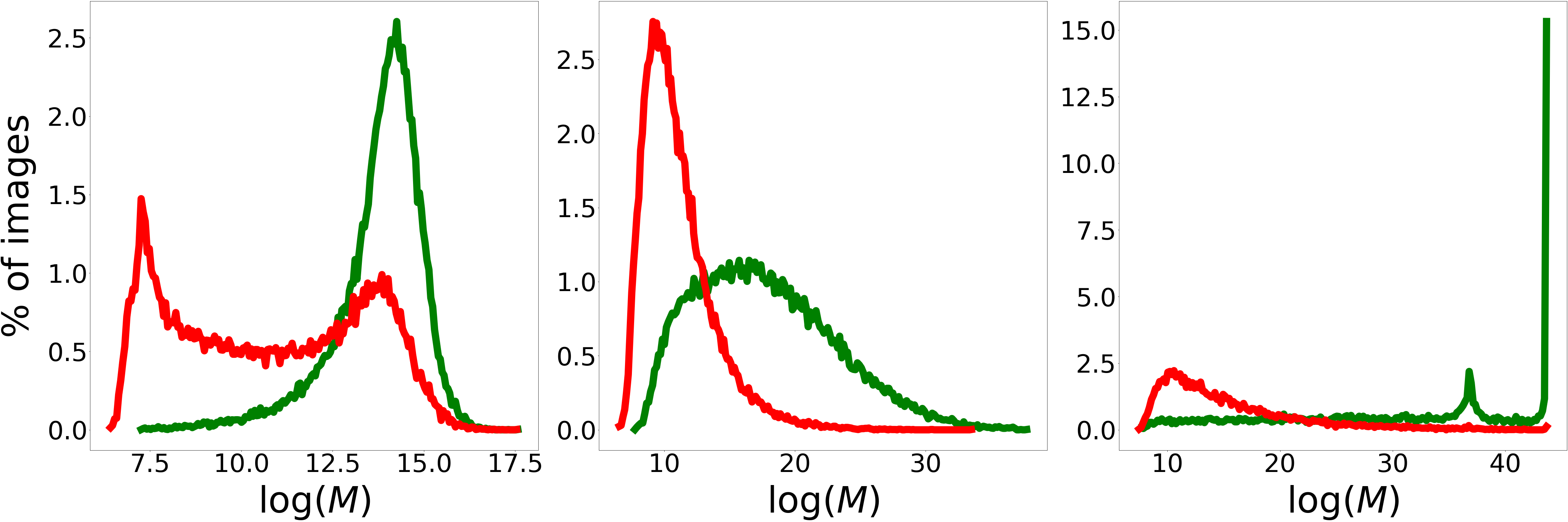
Figure 4: Distribution of values of $\log{(M)}$ for the original clean images (in green) and their Gaussian noise corrupted versions (top row, in red) and Speckle noise corrupted versions (bottom row, in red) obtained from CIFAR-10-C dataset. A distinct nature of the plots for clean and noisy samples can be observed.

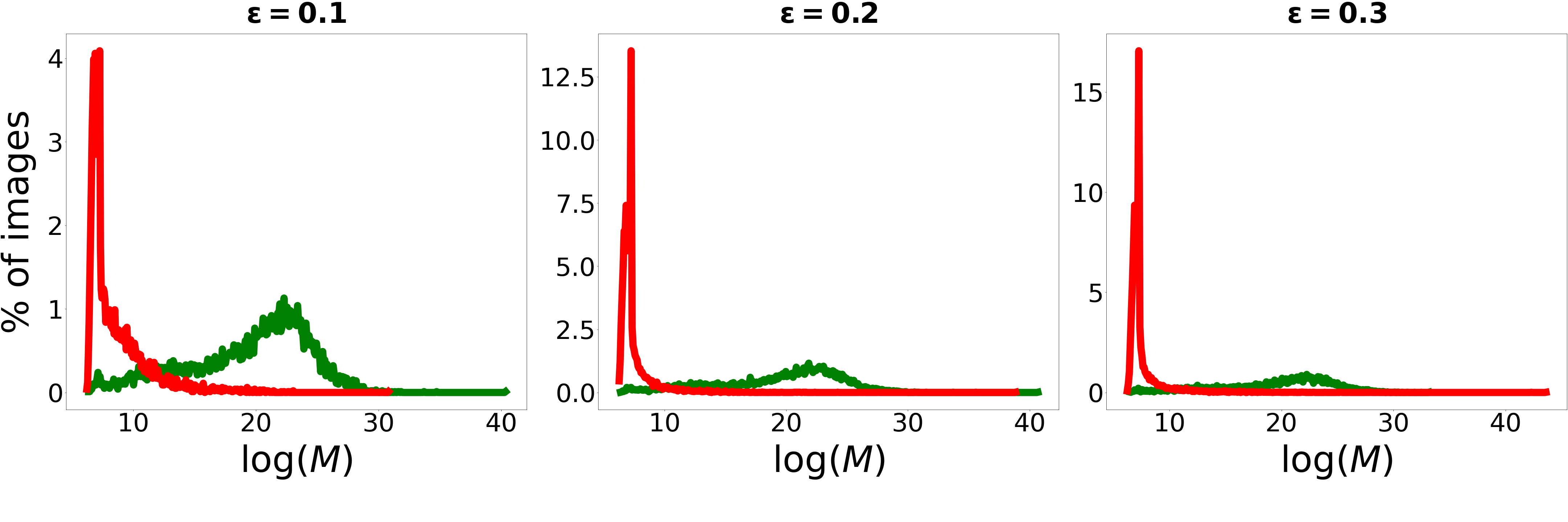
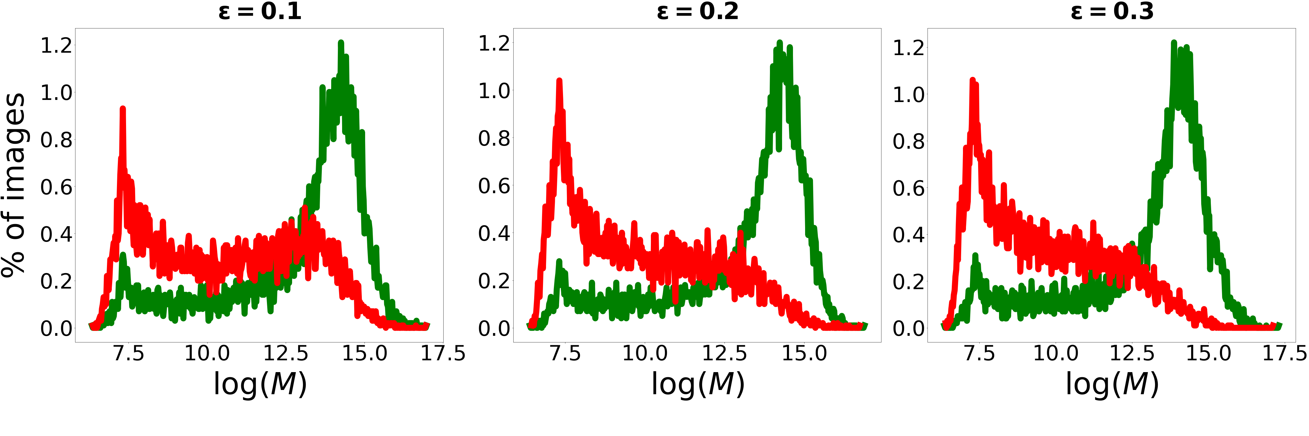
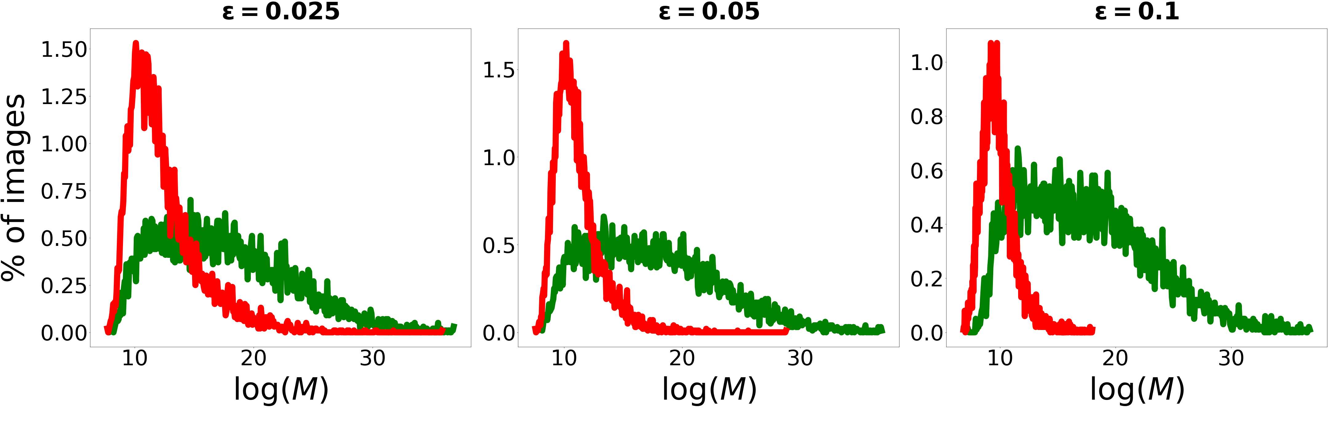
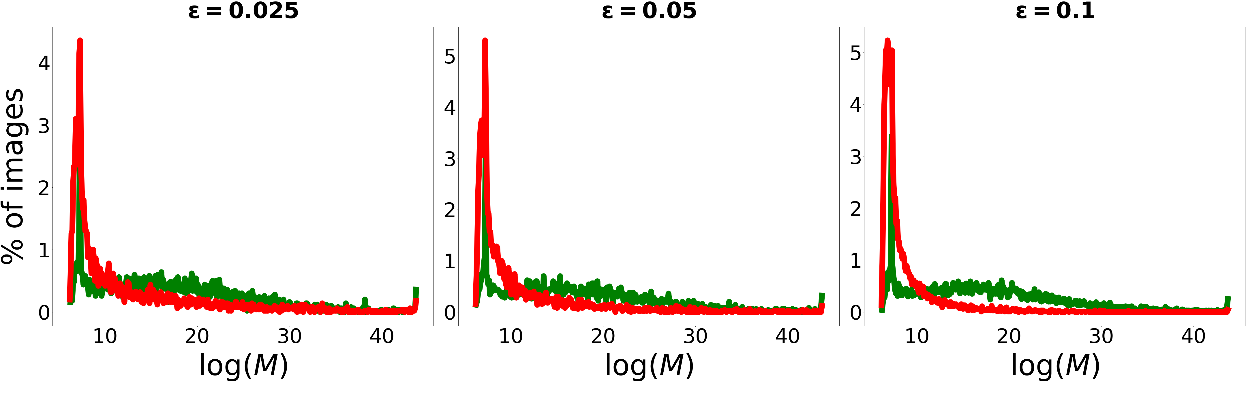
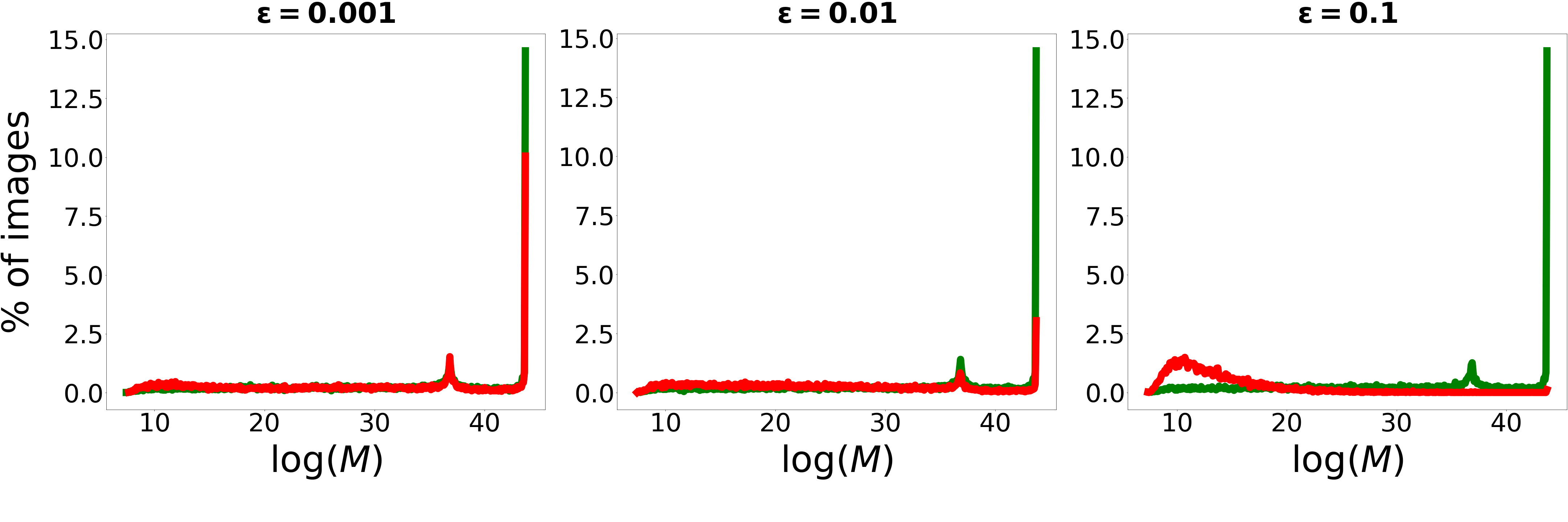
Figure 5: Distribution of $\log{(M)}$ for original images (in green) and their adversarial versions (in red). Rows from top to bottom show the observations for $\operatorname{\mathbb{C}}_{1}$ to $\operatorname{\mathbb{C}}_{5}$, respectively. Peeks of the distribution for original and adversarial images can be easily distinguished from each other. Moreover, with the increase in intensity of adversarial attack ($\epsilon$), the overlap between the distributions decreases. Observe the shift in the red peak with increasing $\epsilon$.

5 Discussion

As mentioned in section 3, proposed probabilistic trust intervals can be interpreted as the space of directed noise. It is, therefore, important to discuss the scenario where instead of learning $\sigma$, a trivial approach is adopted in which small random perturbations are added to the weights of an already trained neural network. We observed in our experiments that this trivial approach results in degradation of test accuracy if the strength of perturbations is too high and if it is too low then test accuracy is preserved but the performance on the task of OOD input detection is suboptimal. For example, when we directly added perturbations sampled from $\mathcal{N}(0,1)$ to the weights of $\operatorname{\mathbb{C}}_{1}$, the test accuracy on MNIST dataset reduced from close to 98% to $\approx$ 10% and when we sampled the perturbations from $\mathcal{N}(0,0.01)$, the FPR at 95% TPR for Fashion-MNIST was $\approx$ 55% which is considerably poor as compared to what is observed for the corresponding PNN, shown in Table 2. In fact, handcrafting the strength of perturbations is nearly impossible because in complex architectures it is very difficult to predict the effect of perturbing weights on the outputs if done manually. Our proposed cost function automates this process and $\sigma$ is learnt in such a way that both the requirements of OOD input detection and test accuracy are satisfied simultaneously.

Further, it is also interesting to discuss the effect of number of siblings on OOD detection. For this we consider PNN corresponding to $\operatorname{\mathbb{C}}_{1}$ trained on MNIST dataset. We sample 2, 5, and 10 values for weight parameters and evaluate the created sets of siblings for ID and OOD (Fashion-MNIST) samples. Similar to the experiments described in previous section, distributions of values of $M$ are plotted in Fig. 6. As we see, the distributions corresponding to OOD samples for different number of weight samples are almost overlapping each other. There is a little improvement with increasing number of weight samples in the performance on ID data. Overall the plots show that 2 samples is a reasonable choice to get the desired results while keeping the amount of computation during inference under control.

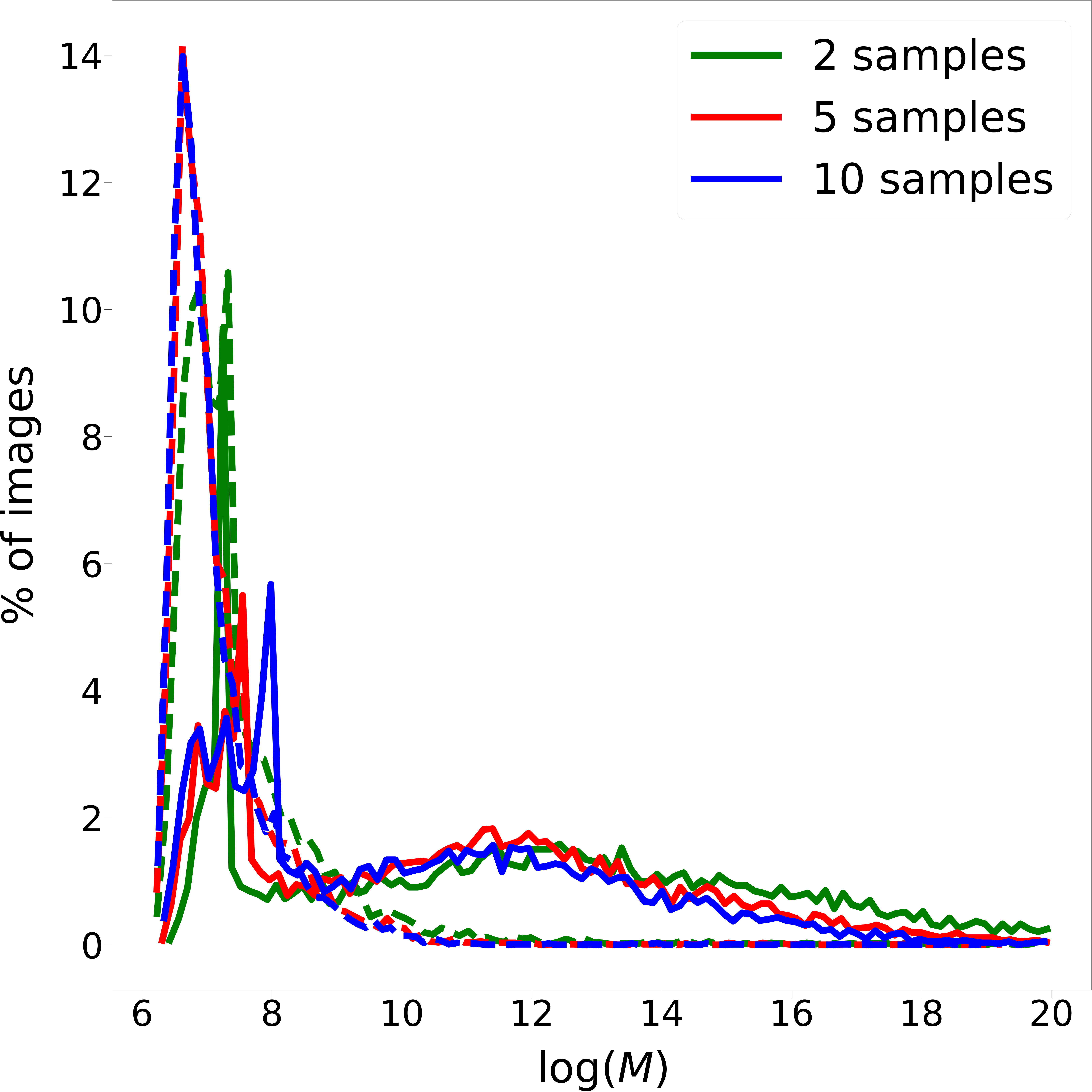
Figure 6: Distribution of $\log{(M)}$ values for $\operatorname{\mathbb{C}}_{1}$ architecture with MNIST dataset as ID data (solid lines) and Fashion-MNIST as OOD data (dashed lines) for different number of weight samples. It can be seen that the distributions almost overlap with each other for different number of samples taken.

6 Conclusion

In this paper, we propose a simple approach to enable OOD detection on already trained deep neural network classifiers using the defined probabilistic trust intervals and optimized for ID data around each weight parameter. We also designed a measure of agreement for a robust detection using the resultant PNNs. Once trained PNN can be safely deployed with a constant memory and computation overhead. PNNs are able to distinguish adversarial and noisy inputs as well. We have used Gaussian distribution to model the probabilistic nature of the trust interval, in future other distributions can also be considered. Another possible future direction is to explore the possibility of removing redundant and very small sized intervals to reduce both, the time consumed in sampling and memory required to store interval parameters. PNNs can also be explored for uncertainty estimation in applications such as regression and segmentation.

References

- [1] Dario Amodei, Chris Olah, Jacob Steinhardt, Paul Christiano, John Schulman, and Dan Mané. Concrete problems in ai safety. arXiv preprint arXiv:1606.06565, 2016.
- [2] Jeremy Bernstein, Jiawei Zhao, Markus Meister, Ming-Yu Liu, Anima Anandkumar, and Yisong Yue. Learning compositional functions via multiplicative weight updates. Advances in Neural Information Processing Systems, 33, 2020.
- [3] Charles Blundell, Julien Cornebise, Koray Kavukcuoglu, and Daan Wierstra. Weight uncertainty in neural network. In International Conference on Machine Learning, pages 1613–1622. PMLR, 2015.
- [4] Kumar Chellapilla, Sidd Puri, and Patrice Simard. High performance convolutional neural networks for document processing. 2006.
- [5] Kyunghyun Cho, Bart Van Merriënboer, Caglar Gulcehre, Dzmitry Bahdanau, Fethi Bougares, Holger Schwenk, and Yoshua Bengio. Learning phrase representations using rnn encoder-decoder for statistical machine translation. arXiv preprint arXiv:1406.1078, 2014.
- [6] Nibaran Das, Jagan Mohan Reddy, Ram Sarkar, Subhadip Basu, Mahantapas Kundu, Mita Nasipuri, and Dipak Kumar Basu. A statistical-topological feature combination for recognition of handwritten numerals. Appl. Soft Comput., 12(8):2486–2495, Aug. 2012.
- [7] Zhijie Deng, Xiao Yang, Hao Zhang, Yinpeng Dong, and Jun Zhu. Bayesadapter: Being bayesian, inexpensively and robustly, via bayeisan fine-tuning. arXiv preprint arXiv:2010.01979, 2020.
- [8] Stanislav Fort, Huiyi Hu, and Balaji Lakshminarayanan. Deep ensembles: A loss landscape perspective. arXiv preprint arXiv:1912.02757, 2019.
- [9] Ian J. Goodfellow, Jonathon Shlens, and Christian Szegedy. Explaining and harnessing adversarial examples, 2015.
- [10] Kaiming He, Xiangyu Zhang, Shaoqing Ren, and Jian Sun. Deep residual learning for image recognition. In Proceedings of the IEEE conference on computer vision and pattern recognition, pages 770–778, 2016.
- [11] Dan Hendrycks and Thomas Dietterich. Benchmarking neural network robustness to common corruptions and perturbations. Proceedings of the International Conference on Learning Representations, 2019.
- [12] Dan Hendrycks and Thomas Dietterich. Benchmarking neural network robustness to common corruptions and perturbations. Proceedings of the International Conference on Learning Representations, 2019.
- [13] Dan Hendrycks and Kevin Gimpel. A baseline for detecting misclassified and out-of-distribution examples in neural networks. arXiv preprint arXiv:1610.02136, 2016.
- [14] Dan Hendrycks, Mantas Mazeika, and Thomas Dietterich. Deep anomaly detection with outlier exposure. arXiv preprint arXiv:1812.04606, 2018.
- [15] Gao Huang, Zhuang Liu, Laurens Van Der Maaten, and Kilian Q Weinberger. Densely connected convolutional networks. In Proceedings of the IEEE conference on computer vision and pattern recognition, pages 4700–4708, 2017.
- [16] Diederik P Kingma and Max Welling. Auto-encoding variational bayes, 2014.
- [17] Alex Krizhevsky, Vinod Nair, and Geoffrey Hinton. Cifar-10 (canadian institute for advanced research).
- [18] Alex Krizhevsky, Vinod Nair, and Geoffrey Hinton. Cifar-100 (canadian institute for advanced research).
- [19] Alex Krizhevsky, Ilya Sutskever, and Geoffrey E Hinton. Imagenet classification with deep convolutional neural networks. In F. Pereira, C. J. C. Burges, L. Bottou, and K. Q. Weinberger, editors, Advances in Neural Information Processing Systems, volume 25, pages 1097–1105. Curran Associates, Inc., 2012.
- [20] Balaji Lakshminarayanan, Alexander Pritzel, and Charles Blundell. Simple and scalable predictive uncertainty estimation using deep ensembles. arXiv preprint arXiv:1612.01474, 2016.
- [21] Yann LeCun, Corinna Cortes, and CJ Burges. Mnist handwritten digit database. ATT Labs [Online]. Available: http://yann.lecun.com/exdb/mnist, 2, 2010.
- [22] Kimin Lee, Honglak Lee, Kibok Lee, and Jinwoo Shin. Training confidence-calibrated classifiers for detecting out-of-distribution samples. arXiv preprint arXiv:1711.09325, 2017.
- [23] Kimin Lee, Kibok Lee, Honglak Lee, and Jinwoo Shin. A simple unified framework for detecting out-of-distribution samples and adversarial attacks. In Advances in Neural Information Processing Systems, pages 7167–7177, 2018.
- [24] Shiyu Liang, Yixuan Li, and Rayadurgam Srikant. Enhancing the reliability of out-of-distribution image detection in neural networks. arXiv preprint arXiv:1706.02690, 2017.
- [25] Yuval Netzer, Tao Wang, Adam Coates, Alessandro Bissacco, Bo Wu, and Andrew Y Ng. Reading digits in natural images with unsupervised feature learning. Advances in Neural Information Processing Systems (NIPS), 2011.
- [26] Anh Nguyen, Jason Yosinski, and Jeff Clune. Deep neural networks are easily fooled: High confidence predictions for unrecognizable images. In Proceedings of the IEEE conference on computer vision and pattern recognition, pages 427–436, 2015.
- [27] Aristotelis-Angelos Papadopoulos, Mohammad Reza Rajati, Nazim Shaikh, and Jiamian Wang. Outlier exposure with confidence control for out-of-distribution detection. Neurocomputing, 441:138–150, 2021.
- [28] Jie Ren, Peter J Liu, Emily Fertig, Jasper Snoek, Ryan Poplin, Mark Depristo, Joshua Dillon, and Balaji Lakshminarayanan. Likelihood ratios for out-of-distribution detection. In Advances in Neural Information Processing Systems, pages 14707–14718, 2019.
- [29] Hippolyt Ritter, Aleksandar Botev, and David Barber. A scalable laplace approximation for neural networks. In 6th International Conference on Learning Representations, ICLR 2018-Conference Track Proceedings, volume 6. International Conference on Representation Learning, 2018.
- [30] Karen Simonyan and Andrew Zisserman. Very deep convolutional networks for large-scale image recognition. arXiv preprint arXiv:1409.1556, 2014.
- [31] Sunil Thulasidasan, Gopinath Chennupati, Jeff Bilmes, Tanmoy Bhattacharya, and Sarah Michalak. On mixup training: Improved calibration and predictive uncertainty for deep neural networks. arXiv preprint arXiv:1905.11001, 2019.
- [32] T. Tieleman and G. Hinton. Lecture 6.5—RmsProp: Divide the gradient by a running average of its recent magnitude. COURSERA: Neural Networks for Machine Learning, 2012.
- [33] Yeming Wen, Dustin Tran, and Jimmy Ba. Batchensemble: an alternative approach to efficient ensemble and lifelong learning. arXiv preprint arXiv:2002.06715, 2020.
- [34] Han Xiao, Kashif Rasul, and Roland Vollgraf. Fashion-mnist: a novel image dataset for benchmarking machine learning algorithms. CoRR, abs/1708.07747, 2017.
- [35] Chiyuan Zhang, Samy Bengio, Moritz Hardt, Benjamin Recht, and Oriol Vinyals. Understanding deep learning requires rethinking generalization. arXiv preprint arXiv:1611.03530, 2016.