Axion Quality from Superconformal Dynamics

Abstract

We discuss a possibility that a superconformal dynamics induces the emergence of a global $U(1)_{\rm PQ}$ symmetry to solve the strong CP problem through the axion. Fields spontaneously breaking the $U(1)_{\rm PQ}$ symmetry couple to new quarks charged under the ordinary color $SU(3)_{C}$ and a new $SU(N)$ gauge group. The theory flows into an IR fixed point where the $U(1)_{\rm PQ}$ breaking fields hold a large anomalous dimension leading to the suppression of $U(1)_{\rm PQ}$-violating higher dimensional operators. The spontaneous breaking of the $U(1)_{\rm PQ}$ makes the new quarks massive. The $U(1)_{\rm PQ}$ symmetry is anomalous under the $SU(3)_{C}$ but not under the $SU(N)$ so that the axion couples to only the color $SU(3)_{C}$ and the usual axion potential is generated. We also comment on a model that the $U(1)_{\rm PQ}$ breaking fields are realized as meson superfields in a new supersymmetric QCD.

Introduction.– The strong CP problem is an intriguing puzzle to motivate physics beyond the Standard Model (SM). The current upper bound on the neutron electric dipole moment constrains the absolute value of the QCD vacuum angle $\bar{\theta}$ to be smaller than $10^{-11}$ Baker:2006ts ; Afach:2015sja . Unlike other naturalness problems in the SM, some shifts of $\bar{\theta}$ would not provide a visible change in our world. The most common explanation for the strong CP problem is the introduction of a pseudo-Nambu-Goldstone boson, called axion $a$ Weinberg:1977ma ; Wilczek:1977pj , associated with spontaneous breaking of a global $U(1)$ Peccei-Quinn ($U(1)_{\rm PQ}$) symmetry Peccei:1977hh (for reviews, see e.g. refs. Kim:2008hd ; DiLuzio:2020wdo ). Non-perturbative QCD effects break the $U(1)_{\rm PQ}$ explicitly and generate a potential of the axion whose minimum sets $\bar{\theta}$ to zero. Astrophysical observations provide a lower limit on the $U(1)_{\rm PQ}$ breaking scale, $f_{a}\gtrsim 10^{8}\,\rm GeV$ Chang:2018rso .

A sufficiently small $\bar{\theta}$ requires the $U(1)_{\rm PQ}$ symmetry to be realized to an extraordinary high degree. However, quantum gravity effects do not respect such a global symmetry. We naturally expect $U(1)_{\rm PQ}$-violating higher dimensional operators suppressed by appropriate powers of the Planck scale $M_{\rm Pl}$ Holman:1992us ; Kamionkowski:1992mf ; Barr:1992qq ; Ghigna:1992iv ; Carpenter:2009zs . Although a discrete $\mathbf{Z}_{n}$ symmetry can forbid some of the operators, to suppress sufficiently higher order terms requires $n\gtrsim 10$ which appears very contrived. Other solutions to this axion quality problem have been explored by many authors. They include composite axion models Kim:1984pt ; Choi:1985cb ; Randall:1992ut ; Redi:2016esr ; DiLuzio:2017tjx ; Lillard:2017cwx ; Lillard:2018fdt ; Gavela:2018paw ; Lee:2018yak , models with a gauged symmetry ($e.g.$ $U(1)$) different from the $U(1)_{PQ}$ Cheng:2001ys ; Harigaya:2013vja ; Harigaya:2015soa ; Fukuda:2017ylt ; Fukuda:2018oco ; Ibe:2018hir ; Choi:2020vgb ; Yin:2020dfn , extra dimension models Dienes:1999gw ; Choi:2003wr ; Flacke:2006ad ; Cox:2019rro ; Bonnefoy:2020llz ; 1842866 and heavy axion models Rubakov:1997vp ; Berezhiani:2000gh ; Hook:2014cda ; Fukuda:2015ana ; Gherghetta:2016fhp ; Dimopoulos:2016lvn ; Gherghetta:2020ofz .

In this letter, we explore an alternative approach to the axion quality problem that a superconformal dynamics induces the emergence of the $U(1)_{\rm PQ}$ symmetry. Our model begins with the existence of a discrete $\mathbf{Z}_{N}$ with $N\sim 5$ which ensures that the model respects the $U(1)_{\rm PQ}$ symmetry at the renormalizable level. We introduce a $SU(N)$ supersymmetric gauge theory with (anti-)fundamental quarks, some of which are also charged under the ordinary color $SU(3)_{C}$. The $\mathbf{Z}_{N}$ symmetry is anomaly-free under the $SU(3)_{C}$ as well as the $SU(N)$. All the new quarks couple to fields responsible for the spontaneous $U(1)_{\rm PQ}$ breaking. The theory flows into an IR fixed point where the $U(1)_{\rm PQ}$ breaking fields hold a large anomalous dimension. Then, even if there exist higher dimensional operators dangerously violating the $U(1)_{\rm PQ}$ at the Planck scale, those operators are significantly suppressed at low-energies. The similar mechanism has been discussed in the context of the Nelson-Strassler model to realize quark and lepton mass hierarchies Nelson:2000sn (for a more recent development using the $a$-maximization technique Intriligator:2003jj , see refs. Poland:2009yb ; Craig:2010ip ). According to the AdS/CFT correspondence Maldacena:1997re , the approach is similar to that of the warped extra dimension model discussed in ref. Cox:2019rro . However, to the best of our knowledge, our model is the first 4D calculable realization to utilize a conformal dynamics to suppress $U(1)_{\rm PQ}$-violating higher dimensional operators. The spontaneous breaking of the $U(1)_{\rm PQ}$ makes all the new quarks massive. The new quarks leading to a large anomalous dimension of the $U(1)_{\rm PQ}$ breaking fields also play the role of the so-called KSVZ quarks Kim:1979if ; Shifman:1979if . Since the $U(1)_{\rm PQ}$ symmetry is anomalous under the $SU(3)_{C}$ but not under the $SU(N)$, the axion couples to only the color $SU(3)_{C}$ and the usual axion potential is generated. The $SU(N)$ finally confines and predicts the existence of $SU(N)$ glueballs.

While the $U(1)_{\rm PQ}$ breaking fields are introduced as elementary fields in the main part of the present work, we will also comment on a possibility that they are realized as meson superfields in a new supersymmetric QCD (SQCD). Interestingly, in the magnetic picture of the theory Seiberg:1994pq ; Intriligator:1995au , the coupling of the $U(1)_{\rm PQ}$ breaking fields to dual quarks is automatic.

	$Q_{m}$	$\bar{Q}_{m}$	$Q_{k}$	$\bar{Q}_{k}$	$\Phi$	$\bar{\Phi}$
$SU(N)$	$\mathbf{N}$	$\overline{\mathbf{N}}$	$\mathbf{N}$	$\overline{\mathbf{N}}$	$\mathbf{1}$	$\mathbf{1}$
$U(1)_{\rm PQ}~{}\left(\mathbf{Z}_{N}\right)$	$+1$	$0$	$-1$	$0$	$-1$	$+1$
$U(1)_{R}$	$\frac{N_{f}-N}{N_{f}}$	$\frac{N_{f}-N}{N_{f}}$	$\frac{N_{f}-N}{N_{f}}$	$\frac{N_{f}-N}{N_{f}}$	$\frac{2N}{N_{f}}$	$\frac{2N}{N_{f}}$

Table 1: The charge assignments under the $SU(N)$ gauge group, the $U(1)_{\rm PQ}$ (and $\mathbf{Z}_{N}$) and the anomaly-free $U(1)_{R}$ which determines anomalous dimensions of the fields. Here, $m=1,\cdots,N_{f}/2$ and $k=N_{f}/2+1,\cdots,N_{f}$ where $N_{f}$ is even.

The model.– Let us consider a supersymmetric $SU(N)$ gauge theory with $N_{f}$ vector-like pairs of chiral superfields in the (anti-)fundamental representation, $Q_{I},\bar{Q}_{I}$ $(I=1,\cdots,N_{f})$. Here, $N_{f}$ is assumed to be even. We focus on $\frac{3}{2}N<N_{f}<3N$ where the theory is in conformal window Intriligator:1995au . To implement the QCD axion, we introduce two $SU(N)$ singlet chiral superfields $\Phi,\bar{\Phi}$ charged under the $U(1)_{\rm PQ}$ symmetry. They are coupled to the new $SU(N)$ quarks in the superpotential,

$$W_{Q}=\lambda\Phi Q_{m}\bar{Q}_{m}+\bar{\lambda}\bar{\Phi}Q_{k}\bar{Q}_{k}\ ,$$ (1)

where $\lambda,~{}\bar{\lambda}$ denote dimensionless couplings, $m$ runs from $1$ to $N_{f}/2$ and $k$ runs from $N_{f}/2+1$ to $N_{f}$. These terms explicitly break the original $SU(N_{f})_{L}\times SU(N_{f})_{R}$ flavor symmetries in the theory into $SU(N_{f}/2)_{1}\times SU(N_{f}/2)_{2}$. A subgroup $SU(3)\subset SU(N_{f}/2)_{1}$ is weakly gauged and regarded as the ordinary color $SU(3)_{C}$ in the SM. Barring the effect of this $SU(3)_{C}$, the couplings flow into $\lambda=\bar{\lambda}$ at low-energies. The charge assignments under the $U(1)_{\rm PQ}$ symmetry are summarized in Tab. 1. The $U(1)_{\rm PQ}$ symmetry is not anomalous under the $SU(N)$ but has the $U(1)_{\rm PQ}-SU(3)_{C}-SU(3)_{C}$ anomaly whose coefficient is given by $A_{U(1)_{\rm PQ}-SU(3)_{C}-SU(3)_{C}}=N$. Then, an anomaly-free discrete symmetry $\mathbf{Z}_{N}\subset U(1)_{\rm PQ}$ is realized, which leads to the $U(1)_{\rm PQ}$ symmetry at the renormalizable level. Below, we will discuss Planck-scale suppressed $U(1)_{\rm PQ}$-violating operators, but those operators must respect the $\mathbf{Z}_{N}$ symmetry. The fields $\Phi,\bar{\Phi}$ obtain a non-zero vacuum expectation value (VEV) via the superpotential,

$$W^{\prime}_{X} =\kappa^{\prime}X(2\Phi\bar{\Phi}-f^{\prime 2})\,,$$ (2)

which breaks the $U(1)_{\rm PQ}$ symmetry spontaneously. Here, $X$ is a singlet chiral superfield, $\kappa^{\prime}$ is a dimensionless parameter and $f^{\prime}$ is a constant with a mass dimension.

The gauge theory is in conformal window and believed to have a non-trivial IR fixed point. Here, let us assume the $SU(N)$ gauge coupling $g$, $\lambda$ and $\bar{\lambda}$ approach values at the fixed point and the theory is in the conformal regime between the energy scales $\Lambda$ and $M_{c}$ ($\Lambda>M_{c}$). We will demonstrate the existence of the IR fixed point later. In this regime, the conformal dynamics generates a large anomalous dimension of $\Phi,\bar{\Phi}$ through the superpotential terms of Eq. (1). The wave function renormalization factor of $\Phi$ (and $\bar{\Phi}$) at IR is given by

$$Z_{\Phi}=\left(\frac{M_{c}}{\Lambda}\right)^{-\gamma_{\Phi}}\ ,$$ (3)

where $\gamma_{\Phi}=6\frac{N}{N_{f}}-2$ is the anomalous dimension of $\Phi$ which is exactly determined in terms of the anomaly-free $U(1)_{R}$ charges summarized in Tab. 1. We now canonically normalize $\Phi$ as

$$\Phi=\left(\frac{M_{c}}{\Lambda}\right)^{\gamma_{\Phi}/2}\hat{\Phi}\ ,$$ (4)

whose hat $\hat{~}{}$ denotes a field in the canonical normalization. Then, the superpotential (2) is rewritten in terms of the normalized fields,

$$W_{X} =\kappa\left(\frac{M_{c}}{\Lambda}\right)^{\gamma_{\Phi}}X(2\hat{\Phi}\hat{\bar{\Phi}}-f^{2})\,,$$ (5)

where $\kappa\sim\kappa^{\prime}$ is dimensionless and $f\sim\left(\frac{M_{c}}{\Lambda}\right)^{-\gamma_{\Phi}/2}f^{\prime}$ is a constant with a mass dimension. The $U(1)_{\rm PQ}$ breaking scale is determined by $f$ which also gives the conformal breaking, $M_{c}\sim f$. The wave function renormalization factor of Eq. (3) will play a key role in suppressing $U(1)_{\rm PQ}$-violating higher dimensional operators as we will see below.

Once the $U(1)_{\rm PQ}$ breaking fields $\Phi,\bar{\Phi}$ obtain the VEV, all the new quarks $Q_{I},\bar{Q}_{I}$ become massive, and then the axion-gluon coupling is generated in the effective Lagrangian after the integration of the new quarks,

$$\mathcal{L}_{\rm eff}\supset N\frac{a}{F_{a}}\frac{g_{c}^{2}}{32\pi^{2}}G\tilde{G}\ ,$$ (6)

where $a$ denotes the axion, $G$ is the field strength of the gluon, $\tilde{G}$ is its dual, $g_{c}$ is the QCD gauge coupling constant and $F_{a}/N=\sqrt{2}f/N$ is the axion decay constant. The same axion-gluon coupling is obtained in the KSVZ axion model Kim:1979if ; Shifman:1979if with $N$ flavors of $SU(3)_{C}$ vector-like quarks. Since the $U(1)_{\rm PQ}$ symmetry is not anomalous under the $SU(N)$, the terms in Eq. (1) do not lead to the axion-$SU(N)$ gluon coupling even after the integration of the quarks. The axion potential is obtained via the non-perturbative QCD effect,

$$V\sim m_{\pi}^{2}f_{\pi}^{2}\cos\left(N\frac{a}{F_{a}}\right)\ ,$$ (7)

where $m_{\pi}$ and $f_{\pi}$ are the pion mass and the decay constant respectively and $m_{\pi}^{2}f_{\pi}^{2}=(0.1\,{\rm GeV})^{4}$. Then, the strong CP problem is solved in the ordinary way. After the decoupling of $Q_{I},\bar{Q}_{I}$, the model becomes a $SU(N)$ pure Yang Mills theory. Because of a large gauge coupling of the $SU(N)$ at the fixed point, the theory confines just below the conformal breaking scale $M_{c}$ and predicts heavy $SU(N)$ glueballs and their superpartners.

Axion quality.– To address the axion quality problem, explicit $U(1)_{\rm PQ}$ breaking terms must be highly suppressed compared to the axion potential generated by the non-perturbative QCD effect (7). The most dangerous Planck-scale suppressed operator respecting the $\mathbf{Z}_{N}$ symmetry is the superpotential term such as

$$W_{\cancel{\rm PQ}} \sim\frac{\Phi^{N}}{M_{\rm Pl}^{N-3}}\sim\left(\frac{M_{c}}{\Lambda}\right)^{\frac{N\gamma_{\Phi}}{2}}\frac{\hat{\Phi}^{N}}{M_{\rm Pl}^{N-3}}\ ,$$ (8)

which leads to the scalar potential in supergravity with $e.g.$ the constant term $W=m_{3/2}M_{\rm Pl}^{2}$ of the superpotential via $V\supset-3WW^{*}/M_{\rm Pl}^{2}$,

$$V_{\cancel{\rm PQ}}=\left(\frac{M_{c}}{\Lambda}\right)^{\frac{N\gamma_{\Phi}}{2}}\frac{\kappa_{\cancel{\rm PQ}}\,m_{3/2}\hat{\Phi}^{N}}{M_{\rm Pl}^{N-3}}\ .$$ (9)

Here, $m_{3/2}$ is the gravitino mass, $\kappa_{\cancel{\rm PQ}}$ is a model dependent coefficient, and $\hat{\Phi}$ denotes the scalar component which is the same notation as the chiral superfield for notational simplicity. The $U(1)_{\rm PQ}$-violating axion potential is then obtained as

$$V_{\cancel{\rm PQ}}\supset\left(\frac{M_{c}}{\Lambda}\right)^{N(3N/N_{f}-1)}\frac{\kappa_{\cancel{\rm PQ}}\,m_{3/2}F_{a}^{N}}{M_{\rm Pl}^{N-3}}\cos\left(N\frac{a}{F_{a}}+\varphi\right),$$ (10)

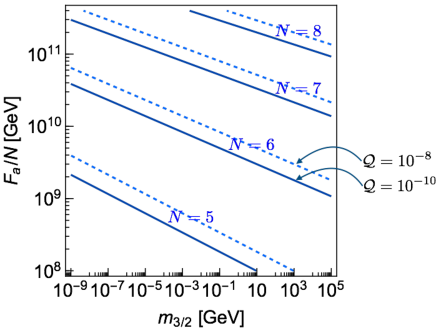
where $\varphi$ denotes a CP phase and $\gamma_{\Phi}=6\frac{N}{N_{f}}-2$ has been used. We now define the axion quality factor $\mathcal{Q}$ by

$$V_{\cancel{\rm PQ}}\equiv\mathcal{Q}\,m_{\pi}^{2}f_{\pi}^{2}\cos\left(N\frac{a}{F_{a}}+\varphi\right).$$ (11)

Assuming $\varphi=\mathcal{O}(1)$, the experimental upper bound on the $\bar{\theta}$ parameter Baker:2006ts ; Afach:2015sja requires $\mathcal{Q}\lesssim 10^{-10}$ to secure the axion quality.

Fig. 1 shows the contours of $\mathcal{Q}$ calculated from the potential (10) in the $m_{3/2}-F_{a}/N$ plane. Here, we take $N_{f}=2\,N$, $M_{c}=F_{a}$, $\kappa_{\cancel{PQ}}=1$, and $\Lambda=0.1\,M_{\rm Pl}$. The solid and dashed lines denote the quality factor $\mathcal{Q}=10^{-10},~{}10^{-8}$, respectively. The axion decay constant $F_{a}/N$ is constrained from the supernova 1981A observation, $F_{a}/N\gtrsim 10^{8}\,{\rm GeV}$ Chang:2018rso . We can see from the figure that there is a parameter space to solve the axion quality problem for $N\geq 5$. While the case of $N=4$ is not shown in the figure, $\mathcal{Q}=10^{-5}$ is obtained for $F_{a}/N\sim 10^{8}$ GeV and $m_{3/2}\sim 1$ eV.

Other potentially dangerous $U(1)_{\rm PQ}$-violating operators are

$$\begin{split}W^{\prime}_{\cancel{\rm PQ}}&\sim\frac{({Q}_{m}{\bar{Q}}_{m})^{N-k}{\bar{\Phi}}^{k}}{M_{\rm Pl}^{2N-k-3}}\\[4.30554pt] &\sim\frac{(\hat{Q}_{m}\hat{\bar{Q}}_{m})^{N-k}\hat{\bar{\Phi}}^{k}}{M_{\rm Pl}^{2N-k-3}}\left(\frac{\Lambda}{M_{c}}\right)^{\gamma_{\Phi}\frac{N-2k}{2}},\end{split}$$ (12)

with $k=0,\cdots,N-1$. While these operators will not lead to the axion potential by themselves, we must be careful because they are enhanced at low-energies due to the negative anomalous dimension of $Q\bar{Q}$. However, for $e.g.$ $N_{f}=2N$, $\Phi~{}(\bar{\Phi})$ and $Q\bar{Q}$ have the same scaling dimension $3/2$, and then Eq. (12) can be rewritten as

$$\begin{split}W^{\prime}_{\cancel{\rm PQ}}&\sim\left(\frac{M_{c}}{\Lambda}\right)^{\frac{N}{2}}\!\!\frac{\hat{\bar{\Phi}}^{N}}{M_{\rm Pl}^{N-3}}\left(\frac{\hat{Q}_{m}\hat{\bar{Q}}_{m}}{\hat{\bar{\Phi}}\,M_{c}}\right)^{N-k}\!\left(\frac{\Lambda}{M_{\rm Pl}}\right)^{N-k},\end{split}$$ (13)

which is suppressed compared to Eq. (8) for $\langle\hat{\bar{\Phi}}\rangle\approx M_{c}$ and $\Lambda<M_{\rm Pl}$. We also note that $U(1)_{\rm PQ}$-violating operators in the Kähler potential are negligible compared to those in the superpotential.

Figure 1: The contours of the quality factor $\mathcal{Q}$ calculated from the potential (10) in the $m_{3/2}-F_{a}/N$ plane. We take $N_{f}=2\,N$, $M_{c}=F_{a}$, $\kappa_{\cancel{PQ}}=1$ and $\Lambda=0.1\,M_{\rm Pl}$. The solid and dashed lines correspond to the quality factor $\mathcal{Q}=10^{-10},~{}10^{-8}$, respectively.

The IR fixed point.– Let us now discuss the existence of the IR fixed point for the $SU(N)$ gauge coupling $g$ and $\lambda,\bar{\lambda}$ in the superpotential (1). We first ignore the effect of the $SU(3)_{C}$ gauge coupling and solve the renormalization group equations (RGEs) for $g$, $\lambda$ and $\bar{\lambda}$,

$$\begin{split}\frac{dg}{dt}&=-\frac{g^{3}}{2}\frac{b_{0}+\frac{1}{2}\sum_{m}\left(\gamma^{1}_{Q_{m}}+\gamma^{1}_{\bar{Q}_{m}}\right)+\frac{1}{2}\sum_{k}\left(\gamma^{1}_{Q_{k}}+\gamma^{1}_{\bar{Q}_{k}}\right)}{8\pi^{2}-C_{A}g^{2}},\\[4.30554pt] \frac{d\lambda}{dt}&=\frac{\lambda}{2}\left(\gamma^{1}_{\Phi}+\gamma^{1}_{Q_{m}}+\gamma^{1}_{\bar{Q}_{m}}\right),\\[4.30554pt] \frac{d\bar{\lambda}}{dt}&=\frac{\bar{\lambda}}{2}\left(\gamma^{1}_{\bar{\Phi}}+\gamma^{1}_{Q_{k}}+\gamma^{1}_{\bar{Q}_{k}}\right),\end{split}$$ (14)

where $t=\ln(\mu/\Lambda_{0})$ with $\mu$ being the RG scale, $C_{A}=N$ and $b_{0}=3N-N_{f}$. Here, we use the exact NSVZ $\beta$ function Novikov:1983uc ; Novikov:1985ic ; Novikov:1985rd for the RGE of the gauge coupling, while the RGEs of $\lambda$ and $\bar{\lambda}$ are shown at the one-loop level. The anomalous dimensions are given by

$$\begin{split}&\gamma^{1}_{Q_{m}}=\gamma^{1}_{\bar{Q}_{m}}=-\frac{1}{8\pi^{2}}\left(2C_{2}g^{2}-\lambda^{2}\right),\\ &\gamma^{1}_{Q_{k}}=\gamma^{1}_{\bar{Q}_{k}}=-\frac{1}{8\pi^{2}}\left(2C_{2}g^{2}-\bar{\lambda}^{2}\right),\\ &\gamma^{1}_{\Phi}=\frac{1}{8\pi^{2}}\lambda^{2}NN_{f}/2\ ,\\ &\gamma^{1}_{\bar{\Phi}}=\frac{1}{8\pi^{2}}\bar{\lambda}^{2}NN_{f}/2\ ,\end{split}$$ (15)

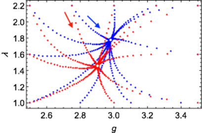
with $C_{2}=\frac{N^{2}-1}{2N}$. We also calculate the RGEs for $\lambda$ and $\bar{\lambda}$ at the two-loop level whose expressions are summarized in appendix. Fig. 2 shows the RG flows of $g$ and $\lambda$ from a scale $\Lambda_{0}$ to $\mu=10^{-9}\Lambda_{0}$ for different initial values as a demonstration. We take $N=5$, $N_{f}=10$ and $\bar{\lambda}=2$ at $\Lambda_{0}$. Blue and red dots correspond to the cases using the one and two-loop RGEs for $\lambda$, respectively. The figure illustrates both couplings flow into a non-trivial IR fixed point. The blue circle around the center denotes the values of $g$ and $\lambda$ obtained by comparing the anomalous dimensions at one-loop (LABEL:eq:gamma_Q_m) to those determined by the $U(1)_{R}$ charges in Tab. 1,

$$\begin{split}&\frac{g_{*}^{2}}{8\pi^{2}}\simeq\frac{N}{N^{2}-1}\frac{\gamma_{\Phi}}{2}\left(1+\frac{2}{NN_{f}/2}\right),\\ &\frac{\lambda_{*}^{2}}{8\pi^{2}}\simeq\frac{\gamma_{\Phi}}{(N_{f}/2)N}\ ,\end{split}$$ (16)

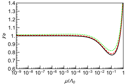
where $\gamma_{\Phi}=6\frac{N}{N_{f}}-2$. The anomalous dimensions up to the two-loop order (27) are used to find the values of the couplings at the red circle. We also plot the anomalous dimension of $\Phi$ at two-loop $\gamma^{2}_{\Phi}$ in the left panel of Fig. 3 (black solid). We take $N=5$, $N_{f}=10$ and $g=\lambda=\bar{\lambda}=2$ at the initial scale $\Lambda_{0}$. The figure indicates that $\gamma^{2}_{\Phi}$ converges to $\gamma_{\Phi}=6\frac{N}{N_{f}}-2=1$. Therefore, the theory is expected to enter the conformal regime in the IR region as we have assumed in the above discussion.

Figure 2: The RG flows of $g$ and $\lambda$ from a scale $\Lambda_{0}$ to $\mu=10^{-9}\Lambda_{0}$ for different initial values. Blue and red dots correspond to the cases using the one and two-loop RGEs for $\lambda$, respectively. The arrows show the directions of the flows. We take $N=5$, $N_{f}=10$ and $\bar{\lambda}=2$ at $\Lambda_{0}$. The blue circle around the center denotes the IR fixed point of Eq. (LABEL:eq:fixed_point) which is obtained by comparing the anomalous dimensions at one-loop (LABEL:eq:gamma_Q_m) to those determined by the $U(1)_{R}$ charges. The anomalous dimensions up to the two-loop order (27) are used to find the values of the couplings at the red circle.

Figure 3: Left panel : The flow of $\gamma^{2}_{\Phi}$ for $g_{c}=0,1,2$ and $g=\lambda_{1}=\lambda_{2}=\bar{\lambda}=2$ at $\Lambda_{0}$ denoted by the black solid, red dashed, green dotted lines, respectively. Right panel : The flow of the wave function renormalization factor $Z_{\Phi}$ for $g_{c}=0,1,2$ and $g=\lambda_{1}=\lambda_{2}=\bar{\lambda}=2$ at $\Lambda_{0}$. The color code and the line style are the same as those of the left panel.

The IR fixed point can be disturbed by the $SU(3)_{C}$ gauge coupling. To discuss this effect, we first decompose the superpotential term in Eq. (1) as

$$W_{Q}\supset\lambda\,Q_{m}\bar{Q}_{m}\to\lambda_{1}\,\Phi Q_{a}\bar{Q}_{a}+\lambda_{2}\,\Phi Q_{\alpha}\bar{Q}_{\alpha}\ ,$$ (17)

where $Q_{a},\bar{Q}_{a}$ $(a=1,2,3)$ denote the fundamental and anti-fundamental representations of the $SU(3)_{C}$ gauge group, $Q_{\alpha},\bar{Q}_{\alpha}$ $(\alpha=4,\cdots,N_{f}/2)$ are the quarks that are not charged under the $SU(3)_{C}$ and $\lambda_{1,2}$ are dimensionless couplings. The anomalous dimensions including the $SU(3)_{C}$ effect at the two-loop level are summarized in appendix. We use the one-loop RGE for the $SU(3)_{C}$ gauge coupling,

$$\frac{dg_{c}}{dt}=-\frac{1}{16\pi^{2}}g_{c}^{3}b_{3}\ ,$$ (18)

which is solved as

$$\frac{4\pi}{g_{c}^{2}}=\left.\frac{4\pi}{g_{c}^{2}}\right|_{\mu=M_{c}}+\frac{b_{3}}{2\pi}\ln(\mu/M_{c})\ ,$$ (19)

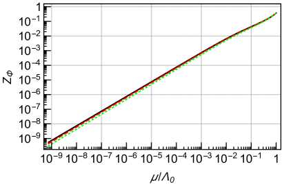
where we take $b_{3}=3-N$ for $\mu>M_{c}$ by assuming all the new quarks have masses around $M_{c}$. Here, the factor $3$ is from the MSSM particles and the factor $-N$ is from the $Q_{a},\bar{Q}_{a}$ quarks. For $N=5$, the $SU(3)_{C}$ gauge coupling becomes asymptotic non-free. In this case, we obtain $g_{c}\approx 1$ around $\mu=10^{17}\,\rm GeV$ for the spectrum of the MSSM particles at about $10\,\rm TeV$ and $4\pi/g_{c}^{2}|_{\mu=M_{c}}\approx 20$ at $M_{c}=10^{8}\,\rm GeV$. We numerically solve the two-loop RGEs from a scale $\Lambda_{0}$ to $\mu=10^{-9}\Lambda_{0}$. The left panel of Fig. 3 shows the flow of $\gamma^{2}_{\Phi}$ for $g_{c}=1,2$ at $\Lambda_{0}$ denoted by the red dashed and green dotted lines, respectively. The initial values of the couplings at $\Lambda_{0}$ are $g=\lambda_{1}=\lambda_{2}=\bar{\lambda}=2$. We also plot the flow of the wave function renormalization factor $Z_{\Phi}$ for $g_{c}=0,1,2,3$ and $g=\lambda_{1}=\lambda_{2}=\bar{\lambda}=2$ at $\Lambda_{0}$ in the right panel of Fig. 3. From the figures, we can confirm that $\gamma^{2}_{\Phi}$ converges into the one without the $SU(3)_{C}$ effect and the smallness of $Z_{\Phi}$ enables to solve the axion quality problem.

A model with the dual picture.– So far, we have discussed the model where the $U(1)_{\rm PQ}$ breaking fields are introduced as elementary fields, but here let us comment on a possibility that they are realized as meson superfields in a new SQCD. Consider a $SU(N_{f}-N)$ SQCD with $N_{f}$ vector-like pairs of quarks whose dual magnetic picture is given by a $SU(N)$ SQCD with the same number of flavors $D_{i},\bar{D}^{i}$ $(i=1,\cdots,N_{f})$ Seiberg:1994pq . In the magnetic theory, there also exist meson chiral superfields $\mathcal{M}^{i}_{j}$ which are coupled to the dual quarks through the superpotential,

$$W_{\rm mag}=y\,\mathcal{M}^{i}_{j}D_{i}\bar{D}^{j}\ ,$$ (20)

where $y$ is a dimensionless coupling. For $\frac{3}{2}N\leq N_{f}\leq 3N$, this gauge theory is in conformal window for both the electric and magnetic pictures and flows into an IR fixed point. We now gauge a diagonal $SU(3)$ subgroup of the $SU(N_{f})_{L}\times SU(N_{f})_{R}$ flavor symmetry in the theory and identify it as the SM color gauge group. For notational convenience, we decompose the mesons $\mathcal{M}^{i}_{j}$ into

$$\mathcal{M}^{i}_{j}=\left(\begin{array}[]{ccc}{\mathcal{M}}^{a}_{1b}&{\mathcal{M}}^{a}_{4\beta}&{\mathcal{M}}^{a}_{6\bar{j}}\\ {\mathcal{M}}^{\alpha}_{5b}&{\mathcal{M}}^{\alpha}_{2\beta}&{\mathcal{M}}^{\alpha}_{8\bar{j}}\\ {\mathcal{M}}^{\bar{i}}_{7b}&{\mathcal{M}}^{\bar{i}}_{9\beta}&{\mathcal{M}}^{\bar{i}}_{3\bar{j}}\end{array}\right),$$ (24)

where $a,b$ ($=1,2,3$) denote the color $SU(3)_{C}$ indices, $\alpha,\beta=4,5,6$ and $\bar{i},\bar{j}=7,\cdots,N_{f}$. The $U(1)_{\rm PQ}$ charges are, for example, assigned as shown in Tab. 2. With these assignments, the $U(1)_{\rm PQ}$ symmetry is not anomalous under the $SU(N)$ but is anomalous under the $SU(3)_{C}$. With the decomposition of Eq. (24), we can see that the superpotential (20) contains the terms similar to those introduced in Eq. (1),

$$W_{\rm mag}\supset y\,\mathcal{M}_{1}D_{a}\bar{D}^{a}+y\,\mathcal{M}_{2}D_{\alpha}\bar{D}^{\alpha}\ .$$ (25)

Here, we have defined $\mathcal{M}_{1}\equiv\frac{1}{3}\mathcal{M}_{1a}^{a}$ and $\mathcal{M}_{2}\equiv\frac{1}{3}\mathcal{M}_{2\alpha}^{\alpha}$. Note that $\mathcal{M}_{1,2}$ are color singlet but $U(1)_{\rm PQ}$ charged. Once they obtain non-zero VEVs, we get the axion-gluon coupling (6). As before, the $U(1)_{\rm PQ}$ symmetry at the renormalizable level is ensured by an anomaly-free $\mathbf{Z}_{N}\subset U(1)_{\rm PQ}$. Explicit $U(1)_{\rm PQ}$-violating higher dimensional operators are suppressed due to large anomalous dimensions of $\mathcal{M}_{1,2}$.

Several comments are in order. The IR fixed point can be disturbed by the $SU(3)_{C}$ gauge interaction. In order to keep the electric/magnetic duality reliable, the values of the couplings in both electric and magnetic pictures at the fixed point must be much larger than the QCD gauge coupling, which requires the theory to be near the middle of conformal window, $N_{f}\approx 2\,N$. Extra meson and quark chiral superfields must get masses appropriately. In particular, $SU(3)_{C}$-charged mesons must be stabilized at the origin to avoid the color breaking. If $\mathcal{M}_{3}\equiv\frac{1}{N_{f}-6}\mathcal{M}_{3\bar{i}}^{\bar{i}}$ obtains a non-zero VEV, all the quarks become massive. Below the scales of $\mathcal{M}_{1,2,3}$ VEVs, the model becomes a confining $SU(N)$ pure Yang Mills theory. Further explorations of this model are left to a future study.

	$D_{a}$	$\bar{D}^{a}$	$D_{\alpha}$	$\bar{D}^{\alpha}$	$D_{\bar{i}}$	$\bar{D}^{\bar{i}}$	$\mathcal{M}_{1}$	$\mathcal{M}_{2}$	$\mathcal{M}_{3}$	$\mathcal{M}_{4}$	$\mathcal{M}_{5}$	$\mathcal{M}_{6}$	$\mathcal{M}_{7}$	$\mathcal{M}_{8}$	$\mathcal{M}_{9}$
$SU(3)_{C}$	$\bar{\mathbf{3}}$	$\mathbf{3}$	$\mathbf{1}$	$\mathbf{1}$	$\mathbf{1}$	$\mathbf{1}$	$\mathbf{Adj.+1}$	$\mathbf{1}$	$\mathbf{1}$	$\mathbf{3}$	$\bar{\mathbf{3}}$	$\mathbf{3}$	$\bar{\mathbf{3}}$	$\mathbf{1}$	$\mathbf{1}$
$U(1)_{\rm PQ}~{}\left(\mathbf{Z}_{N}\right)$	$+1$	$0$	$0$	$-1$	$0$	$0$	$-1$	$+1$	$0$	$0$	$0$	$-1$	$0$	$0$	$+1$

Table 2: The matter content of the magnetic picture of the model and the charge assignments under the color $SU(3)_{C}$ and the $U(1)_{\rm PQ}$ (and $\mathbf{Z}_{N}$). Here, $a$ ($=1,2,3$) denotes the color $SU(3)_{C}$ index, $\alpha=4,5,6$ and $\bar{i}=7,\cdots,N_{f}$.

Conclusions and discussions.– We have considered a possibility that a superconformal dynamics helps to solve the strong CP problem through the axion with a sufficient quality. The $U(1)_{\rm PQ}$ breaking fields are coupled to the new quarks charged under the $SU(3)_{C}$ and the new $SU(N)$. The theory flows into a non-trivial IR fixed point where the $U(1)_{\rm PQ}$ breaking fields hold a large anomalous dimension leading to a strong suppression of explicit $U(1)_{\rm PQ}$ breaking operators. The $U(1)_{\rm PQ}$ is anomalous under the $SU(3)_{C}$ but not under the $SU(N)$ so that the usual axion potential is generated by non-perturbative QCD effects.

The model respects the anomaly-free $\mathbf{Z}_{N}\subset U(1)_{\rm PQ}$, which realizes the $U(1)_{\rm PQ}$ symmetry at the renormalizable level. If the $U(1)_{\rm PQ}$ is spontaneously broken after the end of inflation, cosmic strings are formed at a temperature close to the $U(1)_{\rm PQ}$ breaking scale (see $e.g.$ ref. Kawasaki:2013ae for a review on axion cosmology). Below around the QCD temperature, domain walls attached to the cosmic strings are formed. They are stable due to the $\mathbf{Z}_{N}$ symmetry and cause a cosmological problem. In order to avoid this, the $U(1)_{\rm PQ}$ symmetry must be broken before the end of inflation. In this case, the axion isocurvature perturbation is produced, which leads to a constraint on the Hubble scale of inflation, $H_{\rm inf}\lesssim 10^{7}$ GeV. Cosmological aspects might be an interesting future direction.

We may be able to use the same superconformal dynamics to realize the quark and lepton mass hierarchies in the same way as the Nelson-Strassler model Nelson:2000sn . Such a possibility has been recently discussed in the 5D context Bonnefoy:2020llz . One extra benefit of this scenario is that flavor-dependent soft scalar masses are automatically suppressed Kobayashi:2001kz ; Nelson:2001mq (see also ref. Kobayashi:2010ye ).

References

- (1) C. A. Baker et al., “An Improved experimental limit on the electric dipole moment of the neutron,” Phys. Rev. Lett. 97 (2006) 131801, arXiv:hep-ex/0602020.
- (2) J. M. Pendlebury et al., “Revised experimental upper limit on the electric dipole moment of the neutron,” Phys. Rev. D 92 no. 9, (2015) 092003, arXiv:1509.04411 [hep-ex].
- (3) S. Weinberg, “A New Light Boson?,” Phys. Rev. Lett. 40 (1978) 223–226.
- (4) F. Wilczek, “Problem of Strong and Invariance in the Presence of Instantons,” Phys. Rev. Lett. 40 (1978) 279–282.
- (5) R. D. Peccei and H. R. Quinn, “CP Conservation in the Presence of Instantons,” Phys. Rev. Lett. 38 (1977) 1440–1443.
- (6) J. E. Kim and G. Carosi, “Axions and the Strong CP Problem,” Rev. Mod. Phys. 82 (2010) 557–602, arXiv:0807.3125 [hep-ph]. [Erratum: Rev.Mod.Phys. 91, 049902 (2019)].
- (7) L. Di Luzio, M. Giannotti, E. Nardi, and L. Visinelli, “The landscape of QCD axion models,” Phys. Rept. 870 (2020) 1–117, arXiv:2003.01100 [hep-ph].
- (8) J. H. Chang, R. Essig, and S. D. McDermott, “Supernova 1987A Constraints on Sub-GeV Dark Sectors, Millicharged Particles, the QCD Axion, and an Axion-like Particle,” JHEP 09 (2018) 051, arXiv:1803.00993 [hep-ph].
- (9) R. Holman, S. D. H. Hsu, T. W. Kephart, E. W. Kolb, R. Watkins, and L. M. Widrow, “Solutions to the strong CP problem in a world with gravity,” Phys. Lett. B 282 (1992) 132–136, arXiv:hep-ph/9203206.
- (10) M. Kamionkowski and J. March-Russell, “Planck scale physics and the Peccei-Quinn mechanism,” Phys. Lett. B 282 (1992) 137–141, arXiv:hep-th/9202003.
- (11) S. M. Barr and D. Seckel, “Planck scale corrections to axion models,” Phys. Rev. D 46 (1992) 539–549.
- (12) S. Ghigna, M. Lusignoli, and M. Roncadelli, “Instability of the invisible axion,” Phys. Lett. B 283 (1992) 278–281.
- (13) L. M. Carpenter, M. Dine, and G. Festuccia, “Dynamics of the Peccei Quinn Scale,” Phys. Rev. D 80 (2009) 125017, arXiv:0906.1273 [hep-th].
- (14) J. E. Kim, “A COMPOSITE INVISIBLE AXION,” Phys. Rev. D 31 (1985) 1733.
- (15) K. Choi and J. E. Kim, “DYNAMICAL AXION,” Phys. Rev. D 32 (1985) 1828.
- (16) L. Randall, “Composite axion models and Planck scale physics,” Phys. Lett. B 284 (1992) 77–80.
- (17) M. Redi and R. Sato, “Composite Accidental Axions,” JHEP 05 (2016) 104, arXiv:1602.05427 [hep-ph].
- (18) L. Di Luzio, E. Nardi, and L. Ubaldi, “Accidental Peccei-Quinn symmetry protected to arbitrary order,” Phys. Rev. Lett. 119 no. 1, (2017) 011801, arXiv:1704.01122 [hep-ph].
- (19) B. Lillard and T. M. P. Tait, “A Composite Axion from a Supersymmetric Product Group,” JHEP 11 (2017) 005, arXiv:1707.04261 [hep-ph].
- (20) B. Lillard and T. M. Tait, “A High Quality Composite Axion,” JHEP 11 (2018) 199, arXiv:1811.03089 [hep-ph].
- (21) M. B. Gavela, M. Ibe, P. Quilez, and T. T. Yanagida, “Automatic Peccei–Quinn symmetry,” Eur. Phys. J. C 79 no. 6, (2019) 542, arXiv:1812.08174 [hep-ph].
- (22) H.-S. Lee and W. Yin, “Peccei-Quinn symmetry from a hidden gauge group structure,” Phys. Rev. D 99 no. 1, (2019) 015041, arXiv:1811.04039 [hep-ph].
- (23) H.-C. Cheng and D. E. Kaplan, “Axions and a gauged Peccei-Quinn symmetry,” arXiv:hep-ph/0103346.
- (24) K. Harigaya, M. Ibe, K. Schmitz, and T. T. Yanagida, “Peccei-Quinn symmetry from a gauged discrete R symmetry,” Phys. Rev. D 88 no. 7, (2013) 075022, arXiv:1308.1227 [hep-ph].
- (25) K. Harigaya, M. Ibe, K. Schmitz, and T. T. Yanagida, “Peccei-Quinn Symmetry from Dynamical Supersymmetry Breaking,” Phys. Rev. D 92 no. 7, (2015) 075003, arXiv:1505.07388 [hep-ph].
- (26) H. Fukuda, M. Ibe, M. Suzuki, and T. T. Yanagida, “A ”gauged” Peccei–Quinn symmetry,” Phys. Lett. B 771 (2017) 327–331, arXiv:1703.01112 [hep-ph].
- (27) H. Fukuda, M. Ibe, M. Suzuki, and T. T. Yanagida, “Gauged Peccei-Quinn symmetry — A case of simultaneous breaking of SUSY and PQ symmetry,” JHEP 07 (2018) 128, arXiv:1803.00759 [hep-ph].
- (28) M. Ibe, M. Suzuki, and T. T. Yanagida, “ as a Gauged Peccei-Quinn Symmetry,” JHEP 08 (2018) 049, arXiv:1805.10029 [hep-ph].
- (29) G. Choi, M. Suzuki, and T. T. Yanagida, “QCD axion from a spontaneously broken gauge symmetry,” JHEP 07 (2020) 048, arXiv:2005.10415 [hep-ph].
- (30) W. Yin, “Scale and quality of Peccei-Quinn symmetry and weak gravity conjectures,” JHEP 10 (2020) 032, arXiv:2007.13320 [hep-ph].
- (31) K. R. Dienes, E. Dudas, and T. Gherghetta, “Invisible axions and large radius compactifications,” Phys. Rev. D 62 (2000) 105023, arXiv:hep-ph/9912455.
- (32) K.-w. Choi, “A QCD axion from higher dimensional gauge field,” Phys. Rev. Lett. 92 (2004) 101602, arXiv:hep-ph/0308024.
- (33) T. Flacke, B. Gripaios, J. March-Russell, and D. Maybury, “Warped axions,” JHEP 01 (2007) 061, arXiv:hep-ph/0611278.
- (34) P. Cox, T. Gherghetta, and M. D. Nguyen, “A Holographic Perspective on the Axion Quality Problem,” JHEP 01 (2020) 188, arXiv:1911.09385 [hep-ph].
- (35) Q. Bonnefoy, P. Cox, E. Dudas, T. Gherghetta, and M. D. Nguyen, “Flavoured Warped Axion,” arXiv:2012.09728 [hep-ph].
- (36) M. Yamada and T. T. Yanagida, “A natural and simple UV completion of the QCD axion model,” arXiv:2101.10350 [hep-ph].
- (37) V. A. Rubakov, “Grand unification and heavy axion,” JETP Lett. 65 (1997) 621–624, arXiv:hep-ph/9703409.
- (38) Z. Berezhiani, L. Gianfagna, and M. Giannotti, “Strong CP problem and mirror world: The Weinberg-Wilczek axion revisited,” Phys. Lett. B 500 (2001) 286–296, arXiv:hep-ph/0009290.
- (39) A. Hook, “Anomalous solutions to the strong CP problem,” Phys. Rev. Lett. 114 no. 14, (2015) 141801, arXiv:1411.3325 [hep-ph].
- (40) H. Fukuda, K. Harigaya, M. Ibe, and T. T. Yanagida, “Model of visible QCD axion,” Phys. Rev. D 92 no. 1, (2015) 015021, arXiv:1504.06084 [hep-ph].
- (41) T. Gherghetta, N. Nagata, and M. Shifman, “A Visible QCD Axion from an Enlarged Color Group,” Phys. Rev. D 93 no. 11, (2016) 115010, arXiv:1604.01127 [hep-ph].
- (42) S. Dimopoulos, A. Hook, J. Huang, and G. Marques-Tavares, “A collider observable QCD axion,” JHEP 11 (2016) 052, arXiv:1606.03097 [hep-ph].
- (43) T. Gherghetta and M. D. Nguyen, “A Composite Higgs with a Heavy Composite Axion,” JHEP 12 (2020) 094, arXiv:2007.10875 [hep-ph].
- (44) A. E. Nelson and M. J. Strassler, “Suppressing flavor anarchy,” JHEP 09 (2000) 030, arXiv:hep-ph/0006251.
- (45) K. A. Intriligator and B. Wecht, “The Exact superconformal R symmetry maximizes a,” Nucl. Phys. B 667 (2003) 183–200, arXiv:hep-th/0304128.
- (46) D. Poland and D. Simmons-Duffin, “Superconformal Flavor Simplified,” JHEP 05 (2010) 079, arXiv:0910.4585 [hep-ph].
- (47) N. Craig, “Simple Models of Superconformal Flavor,” arXiv:1004.4218 [hep-ph].
- (48) J. M. Maldacena, “The Large N limit of superconformal field theories and supergravity,” Int. J. Theor. Phys. 38 (1999) 1113–1133, arXiv:hep-th/9711200.
- (49) J. E. Kim, “Weak Interaction Singlet and Strong CP Invariance,” Phys. Rev. Lett. 43 (1979) 103.
- (50) M. A. Shifman, A. I. Vainshtein, and V. I. Zakharov, “Can Confinement Ensure Natural CP Invariance of Strong Interactions?,” Nucl. Phys. B166 (1980) 493–506.
- (51) N. Seiberg, “Electric - magnetic duality in supersymmetric nonAbelian gauge theories,” Nucl. Phys. B 435 (1995) 129–146, arXiv:hep-th/9411149.
- (52) K. A. Intriligator and N. Seiberg, “Lectures on supersymmetric gauge theories and electric-magnetic duality,” Subnucl. Ser. 34 (1997) 237–299, arXiv:hep-th/9509066.
- (53) V. A. Novikov, M. A. Shifman, A. I. Vainshtein, and V. I. Zakharov, “Exact Gell-Mann-Low Function of Supersymmetric Yang-Mills Theories from Instanton Calculus,” Nucl. Phys. B229 (1983) 381–393.
- (54) V. A. Novikov, M. A. Shifman, A. I. Vainshtein, and V. I. Zakharov, “Supersymmetric Instanton Calculus (Gauge Theories with Matter),” Nucl. Phys. B260 (1985) 157–181. [Yad. Fiz.42,1499(1985)].
- (55) V. A. Novikov, M. A. Shifman, A. I. Vainshtein, and V. I. Zakharov, “The beta function in supersymmetric gauge theories. Instantons versus traditional approach,” Phys. Lett. 166B (1986) 329–333. [Sov. J. Nucl. Phys.43,294(1986); Yad. Fiz.43,459(1986)].
- (56) M. Kawasaki and K. Nakayama, “Axions: Theory and Cosmological Role,” Ann. Rev. Nucl. Part. Sci. 63 (2013) 69–95, arXiv:1301.1123 [hep-ph].
- (57) T. Kobayashi and H. Terao, “Sfermion masses in Nelson-Strassler type of models: SUSY standard models coupled with SCFTs,” Phys. Rev. D 64 (2001) 075003, arXiv:hep-ph/0103028.
- (58) A. E. Nelson and M. J. Strassler, “Exact results for supersymmetric renormalization and the supersymmetric flavor problem,” JHEP 07 (2002) 021, arXiv:hep-ph/0104051.
- (59) T. Kobayashi, Y. Nakai, and R. Takahashi, “Revisiting superparticle spectra in superconformal flavor models,” JHEP 09 (2010) 093, arXiv:1006.4042 [hep-ph].