Abstract

A general and comprehensive analysis for the vector currents of two massive particles, $X_{2}$ and $X_{1}$, with arbitrary integer-spin values is given. Our special focus is on the case when two particles are charge self-conjugate, i.e. Majorana bosons. The general structure of their couplings to an on-shell or off-shell vector boson $V$ is described in a manifestly covariant way and then the constraints on the triple vertex due to discrete CP symmetry and the Majorana condition of two particles being Majorana are worked out. The validity of our full analytic investigation is checked by studying the two-body decay, $X_{2}\to VX_{1}$, with an on-shell or off-shell $V$ boson in the helicity formalism complementary to the covariant formulation. Threshold effects of the two-lepton invariant-mass and polar-angle correlations in the two sequential two-body decays, $X_{2}\to VX_{1}$ and $V\to\ell^{-}\ell^{+}$ with $\ell=e$ or $\mu$, are derived analytically in a compact form by use of the Wick helicity rotation and they are investigated numerically in a few specific spin-combination scenarios for probing the spin and dynamical structure of the $X_{2}X_{1}V$ vertex.

1 Introduction

The Standard Model (SM) [1, 2, 3] and beyond contain several particles that are identical to their own antiparticles. In the following, for the sake of a unified description those charge self-conjugate particles are called Majorana bosons or fermions, depending on whether their spins are integer or half-integer, although the term Majorana was used for a charge self-conjugate spin-1/2 fermion originally introduced by Majorana [4] through the formulation of a purely real version of the Dirac equation [5].

Representatively, the spin-0 elementary SM Higgs boson $H$ discovered at the CERN Large Hadron Collider in 2012 [6, 7], various composite mesons such as the spin-0 $\pi^{0}$, the spin-1 $\rho^{0}$ and the spin-2 $a^{0}_{2}$ as well as the spin-1 $J/\psi$, the spin-1 SM isospin-neutral gauge bosons, $\gamma$ and $Z$, and the color-neutral gluons , are Majorana bosons. The presence of Majorana particles is predicted also by various versions of grand-unified theories [8, 9] and it is guaranteed in $N=1$ supersymmetric gauge theories linking bosons to fermions and vice versa [10, 11, 12]. The supersymmetric partners of neutral gauge bosons and Higgs bosons are Majorana fermions. In addition, one of the leading unanswered questions in the context of neutrino physics [13] is whether massive neutrinos are Majorana or Dirac particles. The concept of Majorana particles is ubiquitous in nuclear and particle physics and even in condensed-matter physics [14, 15, 16].

Previously, the electromagnetic properties of two identical-spin particles of possibly different masses and of spin values up to 3/2 have been investigated extensively [17, 18, 19, 20, 21, 22, 23, 24, 25, 26, 27, 28] and those of two identical Majorana particles of arbitrary spin have been worked out in detail in Refs. [29, 30, 31]. In this work, as a natural extension of those previous works and a powerful platform for probing Majorana particles systematically, we provide a general analysis of the vector-current interactions of an on-shell or off-shell vector boson with two massive on-shell integer-spin particles, of which the masses and spins do not have to be identical, and then we elaborate on the special properties of the triple vertex when two particles are Majorana bosons.

The general structure of the vector-current vertex of two Majorana particles and a vector boson can be probed in various production and decay processes at hadron colliders and $e^{-}e^{+}$ colliders [32, 33, 34, 35, 36, 37, 38, 39, 40, 41, 42, 43, 44, 45, 46, 47, 48, 49, 50, 51, 52, 53, 54, 55]. Especially, production of a pair of Majorana particles of arbitrary spins at $e^{-}e^{+}$ colliders and/or two-body (or three-body) decays involving two non-degenerate Majorana particles can serve as a powerful handle for probing the vertex structure [55]. In the present work, as a straightforward and simple check of the validity of our general analytic analysis on the vertex, we make a detailed study of the two-body decay $X_{2}\to VX_{1}$ of a heavier Majorana boson $X_{2}$ into a lighter Majorana boson $X_{1}$ and an on-shell or off-shell vector boson $V$.

This general and model-independent study of the vector currents of two massive (Majorana) particles of arbitrary integer spins coupled to an on-shell or off-shell vector boson can serve as a powerful guide for investigating various interactions among the SM particles and for finding and characterizing new physics beyond the SM (BSM). A similar analysis for half-integer spin particles will be reported separately.

The paper is organized as follows. Firstly, we make a systematic derivation and provide a general analysis of the $X_{2}X_{1}V$ vector-current vertex of two massive on-shell particles, $X_{2}$ and $X_{1}$, of arbitrary integer spins and an on-shell or off-shell vector boson $V$ in a manifestly covariant way in Section 2. This general vertex form is valid irrespective of whether two particles are charged or neutral. The covariant formulation enables us to efficiently derive all the Lorentz-covariant terms of the vertex and to systematically analyze its key characteristics related to discrete CP symmetry or/and the Majorana condition that two particles are charge self-conjugate, i.e. Majorana bosons. Secondly, we check the validity of our covariant description explicitly by analyzing the two-body decay, $X_{2}\to VX_{1}$, with an on-shell or off-shell vector boson $V$ in the helicity formulation originally developed in Ref. [56] and refined and used in a slightly different form later, for example, in Refs. [57, 58, 59] in Section 3. This helicity formalism is equivalent and complementary to the covariant formalism in that it facilitates the enumeration of all the independent terms and the symmetry arguments very efficiently. Thirdly, in combination with the leptonic $V$ decays $V\to\ell^{-}\ell^{+}$ with $\ell=e$ or $\mu$, we investigate the possibility of determining the spin and dynamical structure of the triple vertex through (polar-)angle correlations and/or lepton invariant-mass distributions to be taken into account when the vector boson $V$ has to be unavoidably virtual in Section 4. Finally we summarize our findings and conclude in Section 5.

2 Vertex of two Majorana bosons and a vector boson

An on-shell boson of integer spin $s$, mass $m$, momentum $k$ and helicity $\lambda$ is defined by a rank-$s$ wave tensor $\epsilon^{\alpha_{1}\cdots\alpha_{s}}(k,\lambda)$ [60, 61, 62] that is completely symmetric, traceless and divergence-free

$$\varepsilon_{\mu\nu\alpha_{i}\alpha_{j}}\,\epsilon^{\alpha_{1}\cdots\alpha_{i}\cdots\alpha_{j}\cdots\alpha_{s}}(k,\lambda) = 0\,,$$ (1)

$$g_{\alpha_{i}\alpha_{j}}\,\epsilon^{\alpha_{1}\cdots\alpha_{i}\cdots\alpha_{j}\cdots\alpha_{s}}(k,\lambda) = 0\,,$$ (2)

$$k_{\alpha_{i}}\,\epsilon^{\alpha_{1}\cdots\alpha_{i}\cdots\alpha_{s}}(k,\lambda) = 0\,,$$ (3)

and the wave tensor satisfies the equation $(k^{2}-m^{2})\,\epsilon^{\alpha_{1}\cdots\alpha_{s}}(k,\lambda)=0$ for any helicity value $\lambda$ taking an integer value between $-s$ and $s$. The wave tensor can be expressed explicitly by a linear combination of $s$ products of spin-1 wave vectors with appropriate Clebsch-Gordon coefficients.

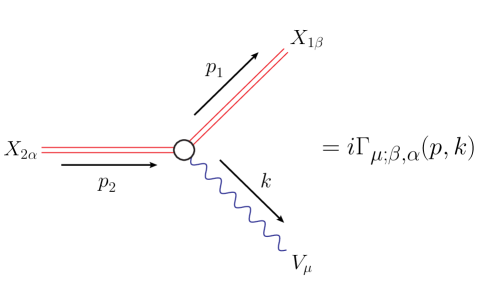
Figure 1: Feynman rules for the general $X_{2}X_{1}V$ vertices of a spin-$s_{2}$ particle $X_{2}$, a spin-$s_{1}$ particle $X_{1}$ and a spin-1 vector boson $V$. The indices, $\beta$ and $\alpha$, stand for the sequences of the $s_{1}$ and $s_{2}$ indices, $\beta=\beta_{1}\cdots\beta_{s_{1}}$ and $\alpha=\alpha_{1}\cdots\alpha_{s_{2}}$, collectively. $p=p_{2}+p_{1}$ and $k=p_{2}-p_{1}$.

The vector currents of two on-shell bosons, $X_{2}$ of mass $m_{2}$ and spin $s_{2}$ and $X_{1}$ of mass $m_{1}$ and spin $s_{1}$, can be written in a general form, which is applicable independently of whether the particles are charged or neutral, as

$$J^{s_{2}s_{1}}_{\mu}(p,k;\lambda_{2},\lambda_{1}) = \langle X_{1}(p_{1},\lambda_{1})|V_{\mu}|X_{2}(p_{2},\lambda_{2})\rangle$$ (4)

$$= \epsilon_{1}^{*\beta_{1}\cdots\beta_{s_{1}}}(p_{1},\lambda_{1})\,\Gamma_{\mu;\beta_{1}\cdots\beta_{s_{1}},\alpha_{1}\cdots\alpha_{s_{2}}}(p,k)\,\,\epsilon_{2}^{\alpha_{1}\cdots\alpha_{s_{2}}}(p_{2},\lambda_{2})\,,$$

$$\bar{J}^{s_{1}s_{2}}_{\mu}(p,k;\lambda_{1},\lambda_{2}) = \langle X_{2}(p_{2},\lambda_{2})|V^{\dagger}_{\mu}|X_{1}(p_{1},\lambda_{1})\rangle$$ (5)

$$= \epsilon_{2}^{*\alpha_{1}\cdots\alpha_{s_{2}}}(p_{2},\lambda_{2})\,\bar{\Gamma}_{\mu;\alpha_{1}\cdots\alpha_{s_{2}},\beta_{1}\cdots\beta_{s_{1}}}(p,k)\,\epsilon_{1}^{\beta_{1}\cdots\beta_{s_{1}}}(p_{1},\lambda_{1})\,,$$

for the $X_{2}\to X_{1}$ and $X_{1}\to X_{2}$ transitions where $p_{1,2}$ and $\lambda_{1,2}$ are the momenta and helicities of the particles, $X_{1,2}$, respectively. Two independent momenta, $p=p_{2}+p_{1}$ and $k=p_{2}-p_{1}$, are introduced for the sake of a systematic and unified description of the two triple vertices. The Feynman rule of the $X_{2}X_{1}V$ interaction vertex is depicted diagrammatically in Figure 1. If any absorptive parts are ignored, the vector vertex operator $V_{\mu}$ is Hermitian, i.e. $V^{\dagger}_{\mu}=V_{\mu}$.

If the currents $J$ and $\bar{J}$ are coupled to an on-shell vector boson $V$ such as a photon $\gamma$ and a massive gauge boson $Z$ or to a conserved vector current through an off-shell $V$ exchange, we can impose the transversality condition

$$k^{\mu}\,J^{s_{2}s_{1}}_{\mu}(p,k;\lambda_{2},\lambda_{1})=0\quad\mbox{and}\quad k^{\mu}\,\bar{J}^{s_{1}s_{2}}_{\mu}(p,k;\lambda_{1},\lambda_{2})=0\,,$$ (6)

with no loss of generality, which effectively kill every term proportional to $k_{\mu}$ in the vertices.

Utilizing the general properties (1), (2) and (3) of the wave tensors, $\epsilon_{1}(p_{1},\lambda_{1})$ and $\epsilon_{2}(p_{2},\lambda_{2})$, let us derive the most general form of the $X_{2}X_{1}V$ vertex, $\Gamma_{\mu;\beta_{1}\cdots\beta_{s_{1}},\alpha_{1}\cdots\alpha_{s_{2}}}(p,k)$, depicted in Figure 1. [For notational convenience, frequently we use $\beta$ and $\alpha$ collectively standing for the sequences of the indices, $\beta_{1}\cdots\beta_{s_{1}}$ and $\alpha_{1}\cdots\alpha_{s_{2}}$.] In the following, we deal with the identical spin case of $s_{2}=s_{1}=s$ and the different spin case of $s_{2}\neq s_{1}$ separately.

2.1 Identical spin case: $s_{2}=s_{1}=s$

If the $X_{2}$ and $X_{1}$ spins are identical, i.e. $s_{2}=s_{1}=s$, the most general form of each of $\Gamma_{\mu;\beta,\alpha}$ and $\bar{\Gamma}_{\mu;\alpha,\beta}$ can be decomposed in six parts as

$$\Gamma_{\mu;\beta_{1}\cdots\beta_{s},\alpha_{1}\cdots\alpha_{s}}(p,k) = p_{\mu}\,F^{1}_{\beta_{1}\cdots\beta_{s},\alpha_{1}\cdots\alpha_{s}}(p,k)+k_{\mu}\,F^{2}_{\beta_{1}\cdots\beta_{s},\alpha_{1}\cdots\alpha_{s}}(p,k)$$ (7)

$$+ (g_{\mu\beta_{1}}p_{\alpha_{1}}+g_{\mu\alpha_{1}}p_{\beta_{1}})\,G^{1}_{\beta_{2}\cdots\beta_{s},\alpha_{2}\cdots\alpha_{s}}(p,k)$$

$$+ \langle\mu\beta_{1}\alpha_{1}k\rangle\,G^{2}_{\beta_{2}\cdots\beta_{s},\alpha_{2}\cdots\alpha_{s}}(p,k)$$

$$+ (g_{\mu\beta_{1}}p_{\alpha_{1}}-g_{\mu\alpha_{1}}p_{\beta_{1}})\,G^{3}_{\beta_{2}\cdots\beta_{s},\alpha_{2}\cdots\alpha_{s}}(p,k)$$

$$+ \langle\mu\beta_{1}\alpha_{1}p\rangle\,G^{4}_{\beta_{2}\cdots\beta_{s},\alpha_{2}\cdots\alpha_{s}}(p,k)\,,$$

$$\bar{\Gamma}_{\mu;\alpha_{1}\cdots\alpha_{s},\beta_{1}\cdots\beta_{s}}(p,k) = \Gamma_{\mu;\beta_{1}\cdots\beta_{s},\alpha_{1}\cdots\alpha_{s}}(p,k)[\,F^{a}\to\bar{F}^{a},\,G^{b}\to\bar{G}^{b}\,]\,,$$ (8)

with the abbreviations, $\langle\mu\beta_{1}\alpha_{1}p\rangle=\varepsilon_{\mu\beta_{1}\alpha_{1}\rho}\,p^{\rho}$ and $\langle\mu\beta_{1}\alpha_{1}k\rangle=\varepsilon_{\mu\beta_{1}\alpha_{1}\rho}\,k^{\rho}$, and the indices, $a=1,2$ and $b=1,2,3,4$, enumerating all the allowed terms. [For future reference, we note here that our convention of the totally antisymmetric Levi-Civita tensor is $\epsilon_{0123}=+1$.] The totally symmetric wave tensors to be coupled to the vertices in Eqs. (7) and (8) guarantee the automatic symmetrization of all the terms including the tensors, $F^{a}(p,k)$, $G^{b}(p,k)$, $\bar{F}^{a}(p,k)$ and $\bar{G}^{b}(p,k)$, under any $\alpha$-index and/or $\beta$-index permutations. 

While the $X_{2}\to X_{1}$ and $X_{1}\to X_{2}$ transition vertices of two spinless particles of $s_{2}=0$ and $s_{1}=0$ have the contribution only from the first two parts in each of Eqs. (7) and (8), the remaining four parts in each equation start participating in constructing the vertices of two Majorana bosons with spin $s\geq 1$.

One crucial point to be exploited for organizing all the independent terms contributing to the triple vertices is that both $p_{\beta}\langle\mu\alpha pk\rangle$ and $p_{\alpha}\langle\mu\beta pk\rangle$ for any 4-vector indices, $\mu,\,\alpha$ and $\beta$, can be expressed in terms of other tensor terms so that they are not independent any more. This can easily be seen as follows. Since no rank-5 completely antisymmetric tensor exists in four dimensions, the following identity holds:

$$g_{\lambda\mu}\varepsilon_{\alpha\beta\rho\sigma}-g_{\lambda\alpha}\varepsilon_{\mu\beta\rho\sigma}+g_{\lambda\beta}\varepsilon_{\mu\alpha\rho\sigma}-g_{\lambda\rho}\varepsilon_{\mu\alpha\beta\sigma}+g_{\lambda\sigma}\varepsilon_{\mu\alpha\beta\rho}=0\,.$$ (9)

By multiplying the above equation by $k^{\lambda}p^{\rho}k^{\sigma}$ and $p^{\lambda}p^{\rho}k^{\sigma}$, we find

$$p_{\beta}\langle\mu\alpha pk\rangle+p_{\alpha}\langle\mu\beta pk\rangle = k_{\mu}\,\langle\beta\alpha pk\rangle+k^{2}\,\langle\mu\beta\alpha p\rangle-p.k\,\langle\mu\beta\alpha k\rangle\,,$$ (10)

$$p_{\beta}\langle\mu\alpha pk\rangle-p_{\alpha}\langle\mu\beta pk\rangle = p_{\mu}\,\langle\beta\alpha pk\rangle-p^{2}\,\langle\mu\beta\alpha k\rangle+p.k\,\langle\mu\beta\alpha p\rangle\,.$$ (11)

Here, $k_{\beta}$ and $k_{\alpha}$ are replaced effectively by $p_{\beta}$ and $-p_{\alpha}$, which is guaranteed by the divergence-free condition (3) of the wave tensors.

The traceless, totally symmetric and divergence-free wave tensors exclude any $g_{\alpha_{i}\alpha_{j}}$ and $g_{\beta_{i}\beta_{j}}$ terms and any $\epsilon_{\alpha_{i}\alpha_{j}\cdots}$ and $\epsilon_{\beta_{i}\beta_{j}\cdots}$ terms. Then, the general form of each of the tensors $F^{a}_{\beta,\alpha}(p,k)$ and $\bar{F}^{a}_{\alpha,\beta}(p,k)$ can be written in terms of mutually independent $s+1$ parity-even and $s$ parity-odd parts as

$$F^{a}_{\beta_{1}\cdots\beta_{s},\alpha_{1}\cdots\alpha_{s}}(p,k) = F^{a}_{1}(k^{2})\,g_{\beta_{1}\alpha_{1}}\cdots g_{\beta_{s}\alpha_{s}}+F^{a}_{2}(k^{2})\,p_{\beta_{1}}p_{\alpha_{1}}g_{\beta_{2}\alpha_{2}}\cdots g_{\beta_{s}\alpha_{s}}$$ (12)

$$+\,\cdots\,+F^{a}_{s+1}(k^{2})\,p_{\beta_{1}}p_{\alpha_{1}}p_{\beta_{2}}p_{\alpha_{2}}\cdots p_{\beta_{s}}p_{\alpha_{s}}$$

$$+F^{\prime a}_{1}(k^{2})\,\langle\beta_{1}\alpha_{1}pk\rangle\,g_{\beta_{2}\alpha_{2}}\cdots g_{\beta_{s}\alpha_{s}}$$

$$+F^{\prime a}_{2}(k^{2})\,\langle\beta_{1}\alpha_{1}pk\rangle\,p_{\beta_{2}}p_{\alpha_{2}}g_{\beta_{3}\alpha_{3}}\cdots g_{\beta_{s}\alpha_{s}}$$

$$+\,\cdots\,+F^{\prime a}_{s}(k^{2})\,\langle\beta_{1}\alpha_{1}pk\rangle\,p_{\beta_{2}}p_{\alpha_{2}}p_{\beta_{3}}p_{\alpha_{3}}\cdots p_{\beta_{s}}p_{\alpha_{s}}\,,$$

$$\bar{F}^{a}_{\alpha_{1}\cdots\alpha_{s},\beta_{1}\cdots\beta_{s}}(p,k) = F^{a}_{\beta_{1}\cdots\beta_{s},\alpha_{1}\cdots\alpha_{s}}(p,k)\,[\,F^{a}_{i}\to\bar{F}^{a}_{i}\ \ \mbox{and}\ \ F^{\prime a}_{j}\to\bar{F}^{\prime a}_{j}\,]\,,$$ (13)

with $a=1,2$, $i=1,\cdots\,s+1$ and $j=1,\cdots\,s$. Similarily, the tensors $G$ and $\bar{G}$ in Eqs. (7) and (8) can be written in terms of $s$ independent parts as

$$G^{b}_{\beta_{2}\cdots\beta_{s},\alpha_{2}\cdots\alpha_{s}}(p,k) = G^{b}_{1}(k^{2})\,g_{\beta_{2}\alpha_{2}}\cdots g_{\beta_{s}\alpha_{s}}+G^{b}_{2}(k^{2})\,p_{\beta_{2}}p_{\alpha_{2}}g_{\beta_{3}\alpha_{3}}\cdots g_{\beta_{s}\alpha_{s}}$$ (14)

$$+\,\cdots\,+G^{b}_{s}(k^{2})\,p_{\beta_{2}}p_{\alpha_{2}}p_{\beta_{3}}p_{\alpha_{3}}\cdots p_{\beta_{s}}p_{\alpha_{s}}\,,$$

$$\bar{G}^{b}_{\alpha_{2}\cdots\alpha_{s},\beta_{2}\cdots\beta_{s}}(p,k) = G^{b}_{\beta_{2}\cdots\beta_{s},\alpha_{2}\cdots\alpha_{s}}(p,k)\,[\,G^{b}_{i}\to\bar{G}^{b}_{i}\,]\,,$$ (15)

for each of $b=1,2,3,4$. It is important to note that substituting the pair $p_{\beta_{j}}p_{\alpha_{j}}$ or $g_{\beta_{j}\alpha_{j}}$ by the symmetric pair $\langle\beta_{j}\alpha_{j}pk\rangle$ with $j\geq 2$ does not introduce any new factor. One immediate consequence of particular importance is that in the identical spin case with $s_{2}=s_{1}=s$ there are in general $8s+2$ independent form factors for each of the $X_{2}\to X_{1}$ and $X_{1}\to X_{2}$ transition vertices of two spin-$s$ on-shell particles $X_{2}$ and $X_{1}$. If the transversality condition is valid, the number of independent terms reduces to $6s+1=(8s+2)-(2s+1)$. Particularly, for the spin $s=1$, there are $6\times 1+1=7$ independent terms as pointed out through the general and comprehensive study of the non-Abelian trilinear $WW\gamma$ and $WWZ$ couplings in Ref. [41].

2.2 Different spin case: $s_{2}\neq s_{1}$

For the sake of convenient discussion on the different spin case, the inequality of $s_{2}>s_{1}$ is assumed without any loss of generality. Then the vertex tensors $\Gamma(p,k)$ and $\bar{\Gamma}(p,k)$ for the $X_{2}\to X_{1}$ and $X_{1}\to X_{2}$ vector-current transitions in Eqs. (4) and (5) can be written as

$$\Gamma_{\mu;\beta_{1}\cdots\beta_{s_{1}},\alpha_{1}\cdots\alpha_{s_{2}}}(p,k) = p_{\mu}\,F^{1}_{\beta_{1}\cdots\beta_{s_{1}},\alpha_{1}\cdots\alpha_{s_{2}}}(p,k)+k_{\mu}\,F^{2}_{\beta_{1}\cdots\beta_{s_{1}},\alpha_{1}\cdots\alpha_{s_{2}}}(p,k)$$ (16)

$$+ (g_{\mu\beta_{1}}p_{\alpha_{1}}+g_{\mu\alpha_{1}}p_{\beta_{1}})\,G^{1}_{\beta_{2}\cdots\beta_{s_{1}},\alpha_{2}\cdots\alpha_{s_{2}}}(p,k)$$

$$+ \langle\mu\beta_{1}\alpha_{1}k\rangle\,G^{2}_{\beta_{2}\cdots\beta_{s_{1}},\alpha_{2}\cdots\alpha_{s_{2}}}(p,k)$$

$$+ (g_{\mu\beta_{1}}p_{\alpha_{1}}-g_{\mu\alpha_{1}}p_{\beta_{1}})\,G^{3}_{\beta_{2}\cdots\beta_{s_{1}},\alpha_{2}\cdots\alpha_{s_{2}}}(p,k)$$

$$+ \langle\mu\beta_{1}\alpha_{1}p\rangle\,G^{4}_{\beta_{2}\cdots\beta_{s_{1}},\alpha_{2}\cdots\alpha_{s_{2}}}(p,k)$$

$$+ g_{\mu\alpha_{1}}\,T_{1}(k^{2})\,g_{\beta_{1}\alpha_{2}}\cdots g_{\beta_{s_{1}}\alpha_{s_{1}+1}}\,p_{\alpha_{s_{1}+2}}\cdots p_{\alpha_{s_{2}}}$$

$$+ \langle\mu\alpha_{1}pk\rangle\,T_{2}(k^{2})\,g_{\beta_{1}\alpha_{2}}\cdots g_{\beta_{s_{1}}\alpha_{s_{1}+1}}\,p_{\alpha_{s_{1}+2}}\cdots p_{\alpha_{s_{2}}}\,,$$

$$\bar{\Gamma}_{\mu;\alpha_{1}\cdots\alpha_{s_{2}},\beta_{1}\cdots\beta_{s_{1}}}(p,-k) = \Gamma_{\mu;\beta_{1}\cdots\beta_{s_{1}},\alpha_{1}\cdots\alpha_{s_{2}}}(p,k)\,[\,F^{a}\to\bar{F}^{a},\,G^{b}\to\bar{G}^{b},\,T_{c}\to\bar{T}_{c}\,]\,,$$ (17)

with $a=1,2$, $b=1,2,3,4$ and $c=1,2$. In passing, we note again that the totally symmetric wave tensors to be coupled to the vertices guarantee the automatic symmetrization of all the terms under any $\alpha$-index and/or $\beta$-index permutations. It is crucial to note that, compared to the identical spin case, there exist two additional form factors in the different spin case, the last two terms in each of Eqs. (16) and (17). With $s_{2}>s_{1}$, the tensors $F$ and $\bar{F}$ can be written in a factorized form as

$$F^{a}_{\beta_{1}\cdots\beta_{s_{1}},\alpha_{1}\cdots\alpha_{s_{2}}}(p,k) = F^{a}_{\beta_{1}\cdots\beta_{s_{1}},\alpha_{1}\cdots\alpha_{s_{1}}}(p,k)\,p_{\alpha_{s_{1}+1}}\cdots p_{\alpha_{s_{2}}}\,,$$ (18)

$$\bar{F}^{a}_{\alpha_{1}\cdots\alpha_{s_{2}},\beta_{1}\cdots\beta_{s_{1}}}(p,k) = \bar{F}^{a}_{\alpha_{1}\cdots\alpha_{s_{1}},\beta_{1}\cdots\beta_{s_{1}}}(p,k)\,p_{\alpha_{s_{1}+1}}\cdots p_{\alpha_{s_{2}}}\,,$$ (19)

with $a=1,2$ where each of the tensors $F^{a}_{\beta_{1}\cdots\beta_{s_{1}},\alpha_{1}\cdots\alpha_{s_{1}}}(p,k)$ and $\bar{F}^{a}_{\alpha_{1}\cdots\alpha_{s_{1}},\beta_{1}\cdots\beta_{s_{1}}}(p,k)$ takes the same form as the expression in each of Eqs. (12) and (13) with the replacement of $s$ by $s_{1}$ in the $s_{2}>s_{1}$ case, i.e. each of the tensors consists of mutually independent $s_{1}+1$ parity-even and $s_{1}$ parity-odd parts. Similarily, each of the tensors $G$ and $\bar{G}$ in Eqs. (16) and (17) also can be factorized as

$$G^{b}_{\beta_{2}\cdots\beta_{s_{1}},\alpha_{2}\cdots\alpha_{s_{2}}}(p,k) = G^{b}_{\beta_{2}\cdots\beta_{s_{1}},\alpha_{2}\cdots\alpha_{s_{1}}}(p,k)\,p_{\alpha_{s_{1}+1}}\cdots p_{\alpha_{s_{2}}}\,,$$ (20)

$$\bar{G}^{b}_{\alpha_{2}\cdots\alpha_{s_{2}},\beta_{2}\cdots\beta_{s_{1}}}(p,k) = \bar{G}^{b}_{\alpha_{2}\cdots\alpha_{s_{1}},\beta_{1}\cdots\beta_{s_{1}}}(p,k)\,p_{\alpha_{s_{1}+1}}\cdots p_{\alpha_{s_{2}}}\,,$$ (21)

with $b=1,2,3,4$ and each of the tensors $G^{b}$ and $\bar{G}^{b}$ consisting of the $s_{1}$ independent parts as the expression in each of Eqs. (14) and (15) with the replacement of $s$ by $s_{1}$. Consequently, in the different spin case of $s_{2}\neq s_{1}$ there are in general $8s+4$ independent form factors with $s={\rm min}(s_{1},s_{2})$ for each of the $X_{2}\to X_{1}$ and $X_{1}\to X_{2}$ transition vertices of a spin-$s_{2}$ on-shell particle $X_{2}$ and a spin-$s_{1}$ on-shell particle $X_{1}$. If the transversality condition is valid, then the number of independent terms reduces to $6s+3=(8s+4)-(2s+1)$.

2.3 Hermiticity and Majorana condition

The results presented in the previous subsections are applicable irrespective of whether the particles $X_{2}$ and $X_{1}$ are charged or neutral. If any absorptive parts are ignored and the particles are charge self-conjugate, i.e. Majorana particles, then the vertex structure is strongly restricted.

Firstly, if any absorptive parts are ignored, i.e. the effective Lagrangian, which is Hermitian, is used for constructing the $X_{2}\to X_{1}$ and $X_{1}\to X_{2}$ transition vector vertices, the following Hermiticity relation holds:

$$\bar{\Gamma}_{\mu;\alpha,\beta}(p,k)\,=\,\Gamma^{*}_{\mu;\beta,\alpha}(p,k)\,.$$ (22)

Independently of whether the particles are charged or neutral, the Hermiticity relation (22) leads to the relations for all the form factors as

$$\bar{F}^{a}_{i}(k^{2}) = F^{a*}_{i}(k^{2})\,,$$ (23)

$$\bar{F}^{\prime a}_{j}(k^{2}) = F^{\prime a*}_{j}(k^{2})\,,$$ (24)

$$\bar{G}^{b}_{j}(k^{2}) = G^{b*}_{j}(k^{2})\,,$$ (25)

$$\bar{T}_{a}(k^{2}) = T^{*}_{a}(k^{2})\,,$$ (26)

where $a=1,2$, $b=1,2,3,4$, $i=1,\cdots,s+1$, and $j=1,\cdots,s$ with $s={\rm min}(s_{2},s_{1})$, so that the $X_{1}\to X_{2}$ transition vertex is fixed once the $X_{2}\to X_{1}$ transition vertex is given.

Secondly, if the particles, $X_{2}$ and $X_{1}$, are not only neutral but also charge self-conjugate, i.e. Majorana bosons, the crossing symmetry gives an additional condition

$$\bar{\Gamma}_{\mu;\alpha,\beta}(p,k)\,=\,\Gamma_{\mu;\beta,\alpha}(-p,-k)\,.$$ (27)

Together with the Hermiticity condition (22), this charge self-conjugation or Majorana relation (27) leads to the condition for the $X_{2}\to X_{1}$ transition (which will be called the Hermiticity-Majorana (HM) condition in the following)

$$\Gamma_{\mu;\beta,\alpha}(p,k)\,=\,\Gamma^{*}_{\mu;\beta,\alpha}(-p,-k)\,,$$ (28)

that is valid independently of whether the spacetime discrete symmetries are conserved or not. It is straightforward to check the following relations of all the form factors

$$F^{a}_{i}(k^{2}) = -\eta_{21}\,F^{a*}_{i}(k^{2})\,,$$ (29)

$$F^{\prime a}_{j}(k^{2}) = -\eta_{21}\,F^{\prime a*}_{j}(k^{2})\,,$$ (30)

$$G^{b}_{j}(k^{2}) = -\eta_{21}\,G^{b*}_{j}(k^{2})\,,$$ (31)

$$T_{a}(k^{2}) = -\eta_{21}\,T^{*}_{a}(k^{2})\,,$$ (32)

with $a=1,2$, $b=1,2,3,4$, $i=1,\cdots,s+1$, and $j=1,\cdots,s$, and with a spin-dependent phase factor $\eta_{21}=(-1)^{s_{2}-s_{1}}$. Therefore, the HM condition (28) leads to the following selection rules:

• In the different spin case, for the even (odd) spin difference case with $\eta_{21}=+1(-1)$, all the $8s+4$ form factors are purely imaginary (purely real).

• In contrast, in the identical spin case always with $\eta_{21}=+1$, the form factors, $T_{1,2}(k^{2})$, are absent. As a result, all the $8s+2$ form factors are purely imaginary.

These selection rules will be demonstrated explicitly by studying the two-body decay $X_{2}\to VX_{1}$ with $V$, collectively denoting an on-shell or off-shell vector boson for four spin combinations of $(s_{2},s_{1})=(0,0),\,(0,1),\,(1,0)$ and $(1,1)$.

If two Majorana bosons, $X_{2}$ and $X_{1}$, are identical, i.e. $s_{2}=s_{1}$ and $m_{2}=m_{1}$, Bose symmetry carries a further requirement that the vertex tensor $\Gamma_{\mu;\beta,\alpha}(p,k)$ be symmetric under the interchange of indices and momenta as $\beta\,\leftrightarrow\,\alpha$ and $p_{1}\,\leftrightarrow\,-p_{2}$, resulting in the replacements, $p\,\rightarrow\,-p$ and $k\,\rightarrow\,k$. In this case, all of the $4s+1$ form factors, $F^{1}_{i}(k^{2})$, $F^{\prime 1}_{j}(k^{2})$ and $G^{1,2}_{j}(k^{2})$, are vanishing and only the $4s+1$ form factors, $F^{2}_{i}(k^{2})$, $F^{\prime 2}_{j}(k^{2})$ and $G^{3,4}_{j}(k^{2})$ can survive. Consequently, we have the following selection rules for the vertex of two identical Majorana bosons worked in detail previously:

• Two identical Majorana spin-zero scalars do not couple to any on-shell vector boson or any conserved vector current at all, as the $F^{2}_{i}(k^{2})$ and $F^{\prime 2}_{j}(k^{2})$ terms do not contribute and the $G^{3,4}_{j}(k^{2})$ terms exist only for $s\geq 1$. It corresponds to the statement that a Majorana scalar cannot have any electromagnetic form factors.

• For the spin $s\geq 1$, every term proportional to $p_{\mu}$ is forbidden, implying that an integer-spin Majorana particle cannot have any static electromagnetic moments.

• All the $2s$ surviving terms are of the so-called anapole type, i.e. they simply give rise to a contact interaction.

All these characteristics are consistent with those derived and discussed in detail in Refs. [30, 31].

If CP symmetry is also preserved in the $X_{2}\leftrightarrow X_{1}$ vector-current transitions, then the following relation combined with the Majorana condition is satisfied:

$$\Gamma_{\mu;\beta,\alpha}(p,k)\,=\,-n^{*}_{2}n_{1}\,\Gamma^{P}_{\mu;\beta,\alpha}(p,k)\,,$$ (33)

with the normalities defined to be $n_{1,2}=\eta_{1,2}\,(-1)^{s_{1,2}}$ in terms of the intrinsic CP parities $\eta_{1,2}$ of the particles, $X_{1,2}$, and under the assumption that the intrinsic CP parity of $V$ is even. The superscript $P$ implying that the sign of every term involving a totally antisymmetric Levi-Civita tensor needs to be flipped. Consequently, CP invariance leads to the following selection rules. In the different spin case, with the same normality of $n_{2}=n_{1}$, only the $4s+1$ parity-odd form factors, $F^{\prime 1,2}_{j}(k^{2})$, $G^{2}_{j}(k^{2})$, $G^{4}_{j}(k^{2})$ and $T_{2}(k^{2})$, survive, and, with the opposite normality of $n_{2}=-n_{1}$, the other $4s+3$ parity-even form factors, $F^{1,2}_{i}(k^{2})$, $G^{1}_{j}(k^{2})$, $G^{3}_{j}(k^{2})$ and $T_{1}(k^{2})$, survive. In the identical spin case, as the form factors $T_{1,2}(k^{2})$ do not appear, the number of independent terms reduce to $4s$ in the same normality case and $4s+2$ in the opposite normality, while if the transversality condition is valid, they further reduce to $3s$ and $3s+1$ in the same and opposite normality cases, respectively.

2.4 The case with $V=\gamma$

When the vector boson $V$ is an on-shell massless photon $\gamma$, the photon wave function and momentum should satisfy the on-shell conditions

$$k\cdot\epsilon_{\gamma}(k,\lambda)=0\quad\mbox{and}\quad k^{2}=0\,,$$ (34)

with the $\gamma$ helicity $\lambda=\pm 1=\pm$. Imposing the on-shell conditions (34) casts the triple vertex $\Gamma$ into the reduced form

$$\Gamma_{\mu;\beta_{1}\cdots\beta_{s_{1}},\alpha_{1}\cdots\alpha_{s_{2}}}(p,k) = (g_{{{}_{\bot}}\mu\beta_{1}}p_{\alpha_{1}}-g_{{{}_{\bot}}\mu\alpha_{1}}p_{\beta_{1}})\,G^{1}_{\beta_{2}\cdots\beta_{s_{1}},\alpha_{2}\cdots\alpha_{s_{2}}}(p,k)$$ (35)

$$+ (g_{{{}_{\bot}}\mu\beta_{1}}p_{\alpha_{1}}+g_{{{}_{\bot}}\mu\alpha_{1}}p_{\beta_{1}})\,G^{2}_{\beta_{2}\cdots\beta_{s_{1}},\alpha_{1}\cdots\alpha_{s_{2}}}(p,k)$$

$$+ \langle\mu\beta_{1}\alpha_{1}k\rangle\,G^{3}_{\beta_{2}\cdots\beta_{s_{1}},\alpha_{1}\cdots\alpha_{s_{2}}}(p,k)$$

$$+ \langle\mu\beta_{1}\alpha_{1}p\rangle_{{}_{\bot}}\,G^{4}_{\beta_{2}\cdots\beta_{s_{1}},\alpha_{1}\cdots\alpha_{s_{2}}}(p,k)$$

$$+ g_{{{}_{\bot}}\mu\alpha_{1}}\,T_{1}(k^{2})\,g_{\beta_{1}\alpha_{2}}\cdots g_{\beta_{s_{1}}\alpha_{s_{1}+1}}\,p_{\alpha_{s_{1}+2}}\cdots p_{\alpha_{s_{2}}}$$

$$+ \langle\mu\alpha_{1}pk\rangle\,T_{2}(k^{2})\,g_{\beta_{1}\alpha_{2}}\cdots g_{\beta_{s_{1}}\alpha_{s_{1}+1}}\,p_{\alpha_{s_{1}+2}}\cdots p_{\alpha_{s_{2}}}\,,$$

with $g_{{{}_{\bot}}\mu\rho}=g_{\mu\rho}-p_{\mu}k_{\rho}/p\cdot k$ for any four-vector index $\rho$, and $\langle\mu\beta\alpha p\rangle_{{}_{\bot}}=\langle\mu\beta\alpha p\rangle+\langle\beta\alpha pk\rangle\,p_{\mu}/p\cdot k$, both of which are orthogonal to $k_{\mu}$. Consequently, in the different and identical spin cases, there are $4s+2$ and $4s$ independent form factors with $s={\rm min}(s_{2},s_{1})$, respectively, as the form factors $T_{1,2}(k^{2})$ do not appear in the identical spin case. In passing, we note that the $X_{2}X_{1}\gamma$ vertex structure for the identical spin case of $s_{2}=s_{1}=1$ has $4\times 1=4$ independent terms as pointed out and studied in detail in Refs. [40, 41, 42, 43, 44, 45, 46, 50].

2.5 The case with $X_{1}=V=\gamma$

As a special case, let us consider the decay of a massive integer-spin Majorana boson into two photons, $X_{2}\to\gamma\gamma$, corresponding to taking $X_{1}=V=\gamma$. Imposing the on-shell conditions

$$p_{1}\cdot\epsilon_{1}(p_{1},\lambda_{1})=0\quad\mbox{and}\quad p^{2}_{1}=0\,,$$ (36)

$$k\cdot\epsilon_{\gamma}(k,\lambda)=0\quad\,\ \ \,\,\mbox{and}\quad k^{2}=0\,,$$ (37)

with $\lambda_{1},\lambda=\pm 1=\pm$, and performing the Bose symmetrization of two identical photon states allow us to write the general $X_{2}\gamma\gamma$ vertex in a greatly-simplified form as

$$\Gamma^{X_{2}\gamma\gamma}_{\mu\beta_{1};\alpha_{1}\cdots\alpha_{s_{2}}}(p_{2},q) = \eta_{+}Y^{+}_{1}\,\,g_{{{}_{\bot}}\mu\beta_{1}}\,\,q_{\alpha_{1}}\cdots q_{\alpha_{s_{2}}}$$ (38)

$$+ \eta_{+}\,Y^{+}_{2}\,\,\langle\mu\beta_{1}p_{2}q\rangle\,\,q_{\alpha_{1}}\cdots q_{\alpha_{s_{2}}}$$

$$+ \eta_{+}\,Y^{+}_{3}\,\,\left[\,g_{{{}_{\bot}}\mu\alpha_{1}}g_{{{}_{\bot}}\beta_{1}\alpha_{2}}+g_{{{}_{\bot}}\beta_{1}\alpha_{1}}g_{{{}_{\bot}}\mu\alpha_{2}}\,\right]\,\,q_{\alpha_{3}}\cdots q_{\alpha_{s_{2}}}$$

$$+ \eta_{-}\,Y^{-}_{1}\,\,\left[\,g_{{}_{\bot}\mu\alpha_{1}}\langle\beta_{1}\alpha_{2}p_{2}q\rangle+g_{{}_{\bot}\beta_{1}\alpha_{1}}\langle\mu\alpha_{2}p_{2}q\rangle\,\right]\,\,q_{\alpha_{3}}\cdots q_{\alpha_{s_{2}}}\,,$$

with the projection factors, $\eta_{\pm}=[1\pm(-1)^{s_{2}}]/2$, and two momentum combinations, $p_{2}=k+p_{1}$ and $q=k-p_{1}$, which are symmetric and antisymmetric under the interchange of two photons, i.e. $k\leftrightarrow p_{1}$ and $\mu\leftrightarrow\beta_{1}$, respectively. For the sake of notation, the following orthogonal tensors are introduced,

$$g_{{}_{\bot}\mu\beta_{1}} = g_{\mu\beta_{1}}-p_{1\mu}k_{\beta_{1}}/p_{1}\cdot k\,,$$ (39)

$$g_{{}_{\bot}\mu\alpha_{i}} = g_{\mu\alpha_{i}}-p_{1\mu}k_{\alpha_{i}}/p_{1}\cdot k\,,$$ (40)

$$g_{{}_{\bot}\beta_{1}\alpha_{i}} = g_{\beta_{1}\alpha_{i}}-k_{\beta_{1}}p_{1\alpha_{i}}/p_{1}\cdot k\,,$$ (41)

with $i=1,2$. The parity of each term in Eq. (38) is determined according to whether its sign flips or not when the sign of $q$ is changed. It is now straightforward to derive the following selection rules from the expression (38) of the $X_{2}\gamma\gamma$ vertex,

• The parity-even $Y^{+}_{1}$ and parity-odd $Y^{+}_{2}$ terms survive for $s_{2}=0,2,4$, etc.

• The parity-even $Y^{+}_{3}$ term survives for $s_{2}=2,4$, etc.

• The parity-even $Y^{-}_{1}$ term survives for $s_{2}=3,5$, etc.

Combining these results together we can count the number $n$ of possible even/odd-parity ($P=\pm$) states of the two-photon system for a given $X_{2}$ integer-spin $s_{2}$. The selection rules can be summarized collectively with the compact notation $n[s_{2}]^{P}$ as

$${\large n\,[s_{2}]^{P}}\ \ =\ \ 1\,[0]^{+}\,,\ \ 2\,[2k]^{+}\,,\ \ 1\,[2k+1]^{+}\,,\ \ 1\,[0]^{-}\,,\ \ 1\,[2k]^{-}\,,$$ (42)

with the positive integer $k=1,2,\cdots$, as worked out independently by Landau [63] and Yang [64]. One immediate consequence of the so-called Landau-Yang theorem is that any massive on-shell spin-1 particle with $s_{2}=1$ cannot decay into two on-shell photons. Accordingly, as the resonance with mass about 125 GeV discovered at the LHC has been observed to decay into two on-shell photons [6, 7], its spin cannot be 1.

3 Decay helicity amplitudes

Complementary to the covariant formalism used in the previous section, the helicity formalism [57, 58, 59] is one of the most effective tools for discussing the two-body decay of an on-shell Majorana particle $X_{2}$ of mass $m_{2}$ and spin $s_{2}$ into an on-shell or off-shell vector boson $V$ of mass $m$ ($=m_{V}$ for an on-shell $V$) and an on-shell Majorana particle $X_{1}$ of mass $m_{1}$ and spin $s_{1}$, irrespective of whether the spins $s_{2}$ and $s_{1}$ are integer or half-integer.

For the sake of a transparent analytic analysis, we describe the two-body decay, $X_{2}\to VX_{1}$,

$$X_{2}(p_{2},\lambda_{2})\ \ \rightarrow\ \ V(k,\lambda)\,+\,X_{1}(p_{1},\lambda_{1})\,,$$ (43)

in the $X_{2}$ rest frame ($X_{2}$RF) and the two-body leptonic decay of an on-shell or off-shell vector boson, $V\to\ell^{-}\ell^{+}$,

$$V(k^{\prime},\lambda^{\prime})\ \ \rightarrow\ \ \ell^{-}(q_{-},\sigma_{-})\,+\ell^{+}(q_{+},\sigma_{+})\,,$$ (44)

in the $V$ rest frame ($V$RF) directly reconstructible event by event by measuring the momenta of two charged leptons with $\ell=e$ or $\mu$ with good precision. The momentum and helicity of each particle are shown in parenthesis with the primed momentum $k^{\prime}$ referring to the momentum in the $V$RF. One crucial point to be taken into account in combining the two sequential decay amplitudes is that the $V$-boson polarization state in the $X_{2}$RF is in general different from that in the $V$RF directly reconstructed in the laboratory frame (LAB).

Before going into a detailed description of the angular correlations in Section 4, we study some general restrictions on the decay helicity amplitudes due to CP invariance and the Majorana condition that the particles, $X_{2}$ and $X_{1}$ are their own antiparticles.

3.1 Correlated decay helicity amplitudes

In general, a virtual vector boson $V$ in its rest frame has a zeroth scalar component as well as three spin-1 space components. However, the scalar component does not contribute to the decay amplitudes meaningfully, if the virtual boson couples to a nearly conserved vector current like the SM $\gamma$ and $Z$ vector currents of the $e$ and $\mu$ leptons due to negligible $e$ and $\mu$ masses. In this light, the transversality condition is assumed to be valid with very good approximation in the following. Then, the $V$ invariant-mass dependent decay helicity amplitude can be decomposed in terms of the polar and azimuthal angles, $\theta$ and $\phi$, of the momentum direction of the boson $V$ in the $X_{2}$RF in the Wick convention as

$${\cal M}^{X_{2}\to VX_{1}}_{\lambda_{2};\lambda,\lambda_{1}}(m;\theta,\phi)={\cal C}_{\lambda,\lambda_{1}}(m)\,d^{s_{2}}_{\lambda_{2},\lambda-\lambda_{1}}(\theta)\,e^{i\lambda_{2}\phi}\quad\mbox{with}\quad|\lambda-\lambda_{1}|\leq s_{2}\,,$$ (45)

with $\lambda_{2}=-s_{2},\cdots,s_{2}$, $\lambda=\pm 1,\,0=\pm,\,0$ and $\lambda_{1}=-s_{1},\cdots,s_{1}$ with the constraint $|\lambda-\lambda_{1}|\leq s_{2}$. The reduced helicity amplitudes ${\cal C}_{\lambda,\lambda_{1}}(m)$ do not depend on any $X_{2}$ helicity $\lambda_{2}$ due to rotational invariance. The polar-angle dependent function $d^{s_{2}}_{\lambda_{2},\lambda-\lambda_{1}}(\theta)$ is a Wigner $d$ function in the convention of Rose [65].

Based on the helicity-amplitude decomposition in Eq. (45) and the restriction of $|\lambda-\lambda_{1}|\leq s_{2}$ on the helicities, it is straightforward to count the number of independent reduced helicity amplitudes even without knowing explicit forms of the reduced helicity amplitudes. In the identical spin case of $s_{2}=s_{1}=s$, two maximal helicity-difference combinations $(\lambda,\lambda_{1})=(\pm 1,\mp s)$ among $(2\times 1+1)\times(2s+1)=6s+3$ combinations of the $V$ and $X_{1}$ helicities are forbidden because of the constraint $|\lambda-\lambda_{1}|\leq s$. As a result, in the identical spin case, the number of independent terms is $6s+1$, the same as counted in the covariant description. On the other hand, if $s_{2}>s_{1}$, the constraint does not play any role so that the number of independent terms is simply $3\times(2s_{1}+1)=6s_{1}+3$. For $s_{2}<s_{1}$, the constraint plays a crucial role in counting the number of degrees of freedom. For $\lambda=0$, the $X_{1}$ helicity $\lambda_{1}$ can take $2s_{2}+1$ values from $-s_{2}$ to $s_{2}$, while for each of $\lambda=\pm 1$, it takes $2s_{2}+1$ values from $-s_{2}\pm 1$ to $s_{2}\pm 1$. Therefore, the number of independent terms is $3\times(2s_{2}+1)=6s_{2}+3$. Consequently, in the different spin case, the number of independent terms is $6s+3$ with $s={\rm min}(s_{2},s_{1})$, the same as counted in the previous covariant description again.

Because generally the momentum direction of the boson $V$ in the $X_{2}$RF is different from that in the laboratory frame (LAB), the helicity amplitude in Eq. (45) needs to be transformed by a proper Wick helicity rotation [54, 58] for connecting the $V$ helicity state in the $X_{2}$RF to that in the LAB with a so-called Wick helicity rotation angle $\omega$ satisfying

$$\cos\omega = \frac{\beta+\beta_{2}\cos\theta}{\sqrt{(1+\beta_{2}\beta\cos\theta)^{2}-(1-\beta^{2}_{2})(1-\beta^{2})}}\,,$$ (46)

$$\sin\omega = \frac{\sqrt{1-\beta^{2}}\,\beta_{2}\sin\theta}{\sqrt{(1+\beta_{2}\beta\cos\theta)^{2}-(1-\beta^{2}_{2})(1-\beta^{2})}}\,,$$ (47)

where $\beta_{2}$ and $\beta$ are the $X_{2}$ speed in the LAB and the $V$ speed in the $X_{2}$RF, which are unambiguously determined in terms of the $X_{2}$ energy in the LAB and the $X_{1,2}$ and $V$ masses. The resulting decay helicity amplitude to be directly coupled with the $V$ decay helicity amplitude in the LAB reads

$${\cal A}_{\lambda_{2};\lambda^{\prime},\lambda_{1}}(\theta,\phi)=\sum_{\lambda=\pm 1,0}\,d^{1}_{\lambda^{\prime},\lambda}(\omega)\,\,{\cal M}^{X_{2}\to VX_{1}}_{\lambda_{2};\lambda,\lambda_{1}}(\theta,\phi)\,,$$ (48)

It is important to note that the Wick helicity rotation angle $\omega$ along with the polar angle $\theta$ is determined event by event, although it might not be possible to determine the azimuthal angle $\phi$ unambiguously.

Among various decay channels of the $V$ boson, if available, the leptonic decays $V\to\ell^{-}\ell^{+}$, especially with $\ell=e$ and $\mu$, can provide a very clean and powerful means for reconstructing the rest frame of the boson $V$, independently of its production mechanisms, and for extracting the information on $V$ polarization efficiently. The helicity amplitude of the leptonic decay to be directly combined with the $X_{2}\to VX_{1}$ helicity amplitude in Eq. (48) can be written as

$${\cal M}^{V\to\ell^{-}\ell^{+}}_{\lambda^{\prime};\,\sigma_{-},\sigma_{+}}(\theta_{\ell},\phi_{\ell})={\cal Z}_{\sigma_{-},\sigma_{+}}(m)\,d^{1}_{\lambda^{\prime},\sigma_{-}-\sigma_{+}}(\theta_{\ell})\,e^{i\lambda^{\prime}\phi_{\ell}}\,,$$ (49)

in terms of the $\ell^{-}$ polar and azimuthal angles, $\theta_{\ell}$ and $\phi_{\ell}$, in the $V$RF with the azimuthal angle which can be defined with respect to the plane formed by the $V$ momentum direction and an appropriately-chosen non-parallel direction fixed in the LAB.

3.2 Discrete spacetime symmetries and Majorana condition

Even in transitions involving weak interactions, the decay processes observe CP symmetry to a great extent while often violating P and C symmetries significantly. So we discuss the consequences of the CP symmetry among discrete spacetime symmetries in the decay helicity amplitudes. For the decay processes involving two Majorana particles $X_{2}$ and $X_{1}$, CP invariance leads to the following relation for the reduced helicity amplitudes in Eq. (45) as

$${\cal C}_{\lambda,\lambda_{1}}(m)=-n^{*}_{2}n_{1}\,\,{\cal C}_{-\lambda,-\lambda_{1}}(m)\,,$$ (50)

with the $X_{2}$ and $X_{1}$ normalities, $n_{2}=\eta_{2}(-1)^{s_{2}}$ and $n_{1}=\eta_{1}(-1)^{s_{1}}$, in terms of the intrinsic CP parities, $\eta_{2}$ and $\eta_{1}$, under the assumption that the normality of $V$ is $-1$ with $s_{V}=1$ and even CP parity like $\gamma$ and $Z$ in the SM. Note that the CP symmetry test does not assume the absence of any absorptive parts and rescattering effects. Certainly, the CP relation (50) of the reduced helicity amplitudes is closely related to the CP relation (33) of the triple vertex tensor.

Together with CPT invariance, the Majorana condition that both of the two neutral particles $X_{2}$ and $X_{1}$ are their own antiparticles leads to the relation for the decay helicity amplitudes in Eq. (45),

$${\cal C}_{\lambda,\lambda_{1}}(m)=-\eta_{21}\,{\cal C}^{*}_{-\lambda,-\lambda_{1}}(m)\,,$$ (51)

with the sign factor $\eta_{21}=(-1)^{s_{2}-s_{1}}$ in the absence of any absorptive parts and rescattering effects. Certainly, this HM relation (51) of the reduced helicity amplitudes reflects the equivalent HM relation (28) of the triple vertex tensors.

As a representative explicit set of the reduced helicity amplitudes, the most general $X_{2}X_{1}V$ tensor couplings for two Majorana particles, $X_{2}$ and $X_{1}$, of spin$\,\,\leq\,1$ are listed in Table 1. The same and opposite normality cases are treated separately, although the analysis in the mixed normality case proceeds as in the fixed normality case, since the most general vertex is the sum of the same and opposite normality cases. For the sake of notation, we use simple alphabetic notations, $a,b,c,d$ and $\bar{a},\bar{b},\bar{c},\bar{d}$ for denoting the independent form factors, dependent generally on the invariant mass $m$ of the on-shell or off-shell vector boson $V$. Taking a specific numerical set of masses and couplings, we present a few numerical analyses for probing the spin and dynamical structure of the two-body decays $X_{2}\to VX_{1}$ directly related to the general $X_{2}X_{1}V$ vertex in Subsection 4.2.

$s_{2},s_{1}$	$X_{2}X_{1}V$ Coupling	Reduced helicity amplitudes	Threshold
Same normality : $n_{2}=n_{1}\,\Rightarrow\,\,{\cal C}_{-\lambda,-\lambda_{1}}=-C_{\lambda,\lambda_{1}}$
$0,0$	+ –	–	–
		$\scriptstyle\ \ {\cal C}_{0,0}\,=\,0$	–
$0,1$	$\phantom{+}b_{1}\,\langle\mu\beta pk\rangle$	$\scriptstyle\ \ {\cal C}_{1,1}\,=\,\imath\,b_{1}\kappa_{*}\,m^{2}_{2}$	$\scriptstyle\kappa_{*}$
		$\scriptstyle\ \ {\cal C}_{0,0}\,=\,0$	–
$1,0$	$\phantom{+}c_{1}\,\langle\mu\alpha pk\rangle$	$\scriptstyle\ \ {\cal C}_{1,0}\,=\,\imath\,c_{1}\kappa_{*}\,m^{2}_{2}$	$\scriptstyle\kappa_{*}$
		$\scriptstyle\ \ {\cal C}_{0,0}\,=\,0$	–
		$\scriptstyle\ \ {\cal C}_{0,1}\,=\,-\imath\,d_{1}(m^{2}_{2}-m^{2}_{1})/m$	$\scriptstyle 1$
	$\phantom{+}d_{1}\,\langle\mu\beta\alpha p\rangle+d_{2}\,\langle\mu\beta\alpha k\rangle$	$\scriptstyle\ \ \phantom{{\cal C}_{0,1}\,=\,}-\imath\,d_{2}m+\imath\,d_{3}\kappa^{2}_{*}\,m^{4}_{2}/m$
$1,1$	$+d_{3}\,\,p_{\mu}\,\langle\beta\alpha pk\rangle$	$\scriptstyle\ \ {\cal C}_{1,0}\,=\,-\imath\,d_{1}(m^{2}_{2}+3m^{2}_{1}-m^{2})/2m_{1}$	$\scriptstyle 1$
		$\scriptstyle\ \ \phantom{{\cal C}_{1,0}\,=\,}-\imath\,d_{2}(m^{2}_{2}-m^{2}_{1}-m^{2})/2m_{1}$
		$\scriptstyle\ \ {\cal C}_{1,1}\,=\,-\imath\,d_{1}(3m^{2}_{2}+m^{2}_{1}-m^{2})/2m_{2}$	$\scriptstyle 1$
		$\scriptstyle\ \ \phantom{{\cal C}_{1,1}\,=\,}-\imath\,d_{2}(m^{2}_{2}-m^{2}_{1}+m^{2})/2m_{2}$
Opposite normality : $n_{2}=-n_{1}\,\Rightarrow\,\,{\cal C}_{-\lambda,-\lambda_{1}}=C_{\lambda,\lambda_{1}}$
$0,0$	$\phantom{+}\bar{a}_{1}\,p_{\mu}$	$\scriptstyle\ \ {\cal C}_{0,0}\,=\,\bar{a}_{1}\kappa_{*}\,m^{2}_{2}/m$	$\scriptstyle\kappa_{*}$
		$\scriptstyle\ \ {\cal C}_{0,0}\,=\,\bar{b}_{1}\,(m^{2}_{2}-m^{2}_{1}-m^{2})/2m_{1}m$	$\scriptstyle 1$
		$\scriptstyle\ \ \phantom{{\cal C}_{0,0}\,=\,}+\bar{b}_{2}\,\kappa^{2}_{*}\,m^{4}_{2}/2m_{1}m$
$0,1$	$\phantom{+}\bar{b}_{1}\,g_{\mu\beta}+\bar{b}_{2}\,p_{\mu}p_{\beta}$	$\scriptstyle\ \ {\cal C}_{1,1}\,=\,-\bar{b}_{1}$	$\scriptstyle 1$
		$\scriptstyle\ \ {\cal C}_{0,0}\,=\,-\bar{c}_{1}\,(m^{2}_{2}-m^{2}_{1}+m^{2})/2m_{2}m$	$\scriptstyle 1$
		$\scriptstyle\ \ \phantom{{\cal C}_{1,0}\,=\,}+\bar{c}_{2}\,\kappa^{2}_{*}\,m^{3}_{2}/2m$
$1,0$	$\phantom{+}\bar{c}_{1}\,g_{\mu\alpha}+\bar{c}_{2}\,p_{\mu}p_{\alpha}$	$\scriptstyle\ \ {\cal C}_{1,0}\,=\,-\bar{c}_{1}$	$\scriptstyle 1$
		$\scriptstyle\ \ {\cal C}_{0,0}\,=\,\bar{d}_{1}\,\kappa_{*}\,m_{2}(m^{2}_{2}+m^{2}_{1}-m^{2})/2m_{1}m$	$\scriptstyle\kappa_{*}$
		$\scriptstyle\ \ \phantom{{\cal C}_{0,0}\,=\,}+\bar{d}_{2}\,\kappa_{*}\,m_{2}(m^{2}_{1}-m^{2})/2m_{1}m$
	$\phantom{+}\bar{d}_{1}\,p_{\mu}g_{\beta\alpha}+\bar{d}_{2}\,(g_{\mu\beta}p_{\alpha}+g_{\mu\alpha}p_{\beta})$	$\scriptstyle\ \ \phantom{{\cal C}_{0,0}\,=\,}+\bar{d}_{3}\,\kappa_{*}\,m_{2}(m^{2}_{2}-m^{2}_{1})/2m_{1}m$
$1,1$	$+\bar{d}_{3}\,(g_{\mu\beta}p_{\alpha}-g_{\mu\alpha}p_{\beta})+\bar{d}_{4}\,p_{\mu}p_{\beta}p_{\alpha}$	$\scriptstyle\ \ \phantom{{\cal C}_{0,0}\,=\,}+\bar{d}_{4}\,\kappa^{3}_{*}\,m^{5}_{2}/4m_{1}m$
		$\scriptstyle\ \ {\cal C}_{0,1}\,=\,\bar{d}_{1}\,\kappa_{*}\,m^{2}_{2}/m$	$\scriptstyle\kappa_{*}$
		$\scriptstyle\ \ {\cal C}_{1,0}\,=\,-(\bar{d}_{2}-\bar{d}_{3})\,\kappa_{*}\,m^{2}_{2}/2m_{1}$	$\scriptstyle\kappa_{*}$
		$\scriptstyle\ \ {\cal C}_{1,1}\,=\,-(\bar{d}_{2}+\bar{d}_{3})\,\kappa_{*}\,m_{2}/2$	$\scriptstyle\kappa_{*}$

Table 1: The most general $X_{2}X_{1}V$ tensor couplings and the corresponding reduced helicity amplitudes for $X_{2}$ and $X_{1}$ of spin $\leq 1$. Here $p=p_{2}+p_{1}$ and $k=p_{2}-p_{1}$, where $p_{2,1}$ and $m_{2,1}$ are the momenta and masses of the on-shell particles, $X_{2}$ and $X_{1}$, and $m=\sqrt{k^{2}}$. The kinematical factor $\kappa_{*}=\lambda^{1/2}(1,m^{2}_{1}/m^{2}_{2},m^{2}/m^{2}_{2})$ related to the $V$ speed in the $X_{2}$RF is approximately proportional to $\sqrt{(m_{2}-m_{1})-m}$ just below the threshold. Note that the reduced helicity amplitudes, ${\cal C}_{00}$, are vanishing in the same normality case as these decay modes are forbidden due to angular momentum conservation .

4 Correlated invariant-mass and polar-angle distributions

The fully-correlated decay amplitudes will be helpful for probing the polarization phenomena through which the spin and dynamical structures of the interaction vertices are decoded. In this section, firstly we derive all the analytic expressions for the correlated invariant-mass and polar-angle distributions for the two sequential decays, $X_{2}\to VX_{1}$ and $V\to\ell^{-}\ell^{+}$ with $\ell=e$ and $\mu$, which consist of two helicity-dependent parts. Secondly, we check all the analytic results by analyzing four different spin combinations of $(s_{2},s_{1})=(0,0),(0,1),(1,0)$ and $(1,1)$ numerically in two sets of masses, of which one set is for an off-shell $V$ and the other set for an on-shell $V$.

4.1 Analytic derivation of the correlated distributions

We assume that the decaying $X_{2}$ particle is unpolarized on average  but it may have a known energy profile. As pointed out before, it is necessary to include a Wick helicity rotation for calculating the combined helicity amplitude of the sequential decay of two 2-body decays $X_{2}\to VX_{1}$ and $V\to\ell^{-}\ell^{+}$ with $\ell=e$ or $\mu$. Note that the polar angle $\theta_{\ell}$ of the charged lepton $\ell^{-}$ in the decay $V\to\ell^{-}\ell^{+}$ can be measured event by event and so the $\theta_{\ell}$ distribution can be determined unambiguously. Integrating the distribution over the lepton azimuthal angle $\phi_{\ell}$, which is usually difficult to be reconstructed, casts the $V$ leptonic-decay density matrix depending on the reconstructible polar angle $\theta_{\ell}$ into a diagonal form

$$\rho^{V}_{\lambda^{\prime},\lambda^{\prime}}(\theta_{\ell})=\frac{1}{4}\,{\rm diag}\left(1+\cos^{2}\theta_{\ell}+2A_{\ell}\,\cos\theta_{\ell},\ \ 2\sin^{2}\theta_{\ell},\ \ 1+\cos^{2}\theta_{\ell}-2A_{\ell}\,\cos\theta_{\ell}\right)\,,$$ (52)

in the $(+1,0,-1)$ basis with the parity-odd factor $A_{\ell}=2v_{\ell}a_{\ell}/(v^{2}_{\ell}+a^{2}_{\ell})$ in terms of the normalized $V\ell\ell$ vector and axial-vector couplings $v_{\ell}$ and $a_{\ell}$. Numerically, for $V=Z$, $A_{\ell}\simeq-0.16$ [66]. Then, the correlated invariant-mass and polar-angle distribution independent of the production mechanism reads

$$\frac{d\Gamma[X_{2}\to VX_{1}\to\ell^{-}\ell^{+}X_{1}]}{dm\,d\cos\theta\,d\cos\theta_{\ell}} = \frac{2m^{3}}{(m^{2}-m^{2}_{V})^{2}+m^{2}_{V}\Gamma^{2}_{V}}\,\frac{d{\cal D}[X_{2}\to VX_{1}\to\ell^{-}\ell^{+}X_{1}]}{d\cos\theta\,d\cos\theta_{\ell}}\,,$$ (53)

where the correlated polar-angle distribution is given by

$$\frac{d{\cal D}[X_{2}\to VX_{1}\to\ell^{-}\ell^{+}X_{1}]}{d\cos\theta\,d\cos\theta_{\ell}} = \frac{3\kappa_{*}\,\Gamma[V\to\ell^{-}\ell^{+}](m)}{64(2s_{2}+1)\pi^{2}m_{2}\,m}\sum_{\lambda^{\prime},\lambda,\lambda_{1}}[d^{1}_{\lambda^{\prime},\lambda}(\omega)|^{2}\,|C_{\lambda,\lambda_{1}}(m)|^{2}\,\rho^{V}_{\lambda^{\prime},\lambda^{\prime}}(\theta_{\ell})$$ (54)

$$= \frac{3\Gamma[V\to\ell^{-}\ell^{+}](m_{V})}{64(2s_{2}+1)\pi^{2}m_{2}\,m_{V}}\,\kappa_{*}\,\sum_{\lambda^{\prime}}\,W_{\lambda^{\prime},\lambda^{\prime}}(m,\omega)\,\rho^{V}_{\lambda^{\prime},\lambda^{\prime}}(\theta_{\ell})\,,$$

with $\lambda^{\prime},\lambda=\pm 1,0$ and $\lambda_{1}=-s_{1},\cdots,s_{1}$ satisfying the constraint $|\lambda-\lambda_{1}|\leq s_{2}$ and with the kinematical phase factor $\kappa_{*}=\lambda^{1/2}(1,m^{2}/m^{2}_{2},m^{2}_{1}/m^{2}_{2})$. In the last expression, we have taken into account the fact that $\Gamma[V\to\ell^{-}\ell^{+}](m)$ scales in proportion to the invariant mass $m$, when the lepton masses are ignored. For the sake of discussion, the so-called Wick distribution function (WDF) $W_{\lambda^{\prime},\lambda^{\prime}}(m,\omega)$ as defined in Ref. [54] is introduced:

$$W_{\lambda^{\prime},\lambda^{\prime}}(m,\omega)=\sum_{\lambda,\lambda_{1}}\,[\,d^{1}_{\lambda^{\prime},\lambda}(\omega)]^{2}\,|C_{\lambda,\lambda_{1}}(m)|^{2}\,,$$ (55)

with the constraint $|\lambda-\lambda_{1}|\leq s_{2}$, where $\omega$ is a function of not only $\cos\theta$ but also $m$ as can be checked with Eqs. (46) and (47). This WDF encodes the information on the spin and dynamical structure of the two-body decay $X_{2}\to VX_{1}$ fully.

If the mass difference $m_{2}-m_{1}$ is larger than the vector-boson mass $m_{V}$ and also the width $\Gamma_{V}$ is much smaller than the mass $m_{V}$, we can take the narrow-width approximation (NWA),

$$\frac{2m^{3}}{(m^{2}-m^{2}_{V})^{2}+m^{2}_{V}\Gamma^{2}_{V}}\quad\rightarrow\quad\pi\,\frac{m_{V}}{\Gamma_{V}}\,\delta(m-m_{V})\,,$$ (56)

and then the correlated polar-angle distribution and the total width are given by

$$\frac{d\Gamma[X_{2}\to VX_{1}\to\ell^{-}\ell^{+}X_{1}]}{d\cos\theta\,d\cos\theta_{\ell}} = \frac{3\,{\rm Br}[V\to\ell^{-}\ell^{+}]}{64(2s_{2}+1)\pi m_{2}}\,\,\kappa\,\sum_{\lambda^{\prime}}\,W_{\lambda^{\prime},\lambda^{\prime}}(m_{V},\omega)\,\rho^{V}_{\lambda^{\prime},\lambda^{\prime}}(\theta_{\ell})\,,$$ (57)

$$\Gamma[X_{2}\to VX_{1}\to\ell^{-}\ell^{+}X_{1}] = \frac{{\rm Br}[V\to\ell^{-}\ell^{+}]}{16(2s_{2}+1)\pi m_{2}}\,\,\kappa\,\sum_{\lambda,\lambda_{1}}\,|\,{\cal C}_{\lambda,\lambda_{1}}(m_{V})|^{2}\,,$$ (58)

with the constraint $|\lambda-\lambda_{1}|\leq s_{2}$ and the kinematical factor $\kappa=\lambda^{1/2}(1,m^{2}_{1}/m^{2}_{2},m^{2}_{V}/m^{2}_{2})$.

The normalized invariant-mass and correlated polar-angle distributions, which are valid for any value of the mass difference $m_{2}-m_{1}$ are

$$\frac{dN(m)}{dm}\!\! = \!\!\frac{\Pi_{V}(m)\,\,\kappa_{*}\,\sum_{\lambda,\lambda_{1}}|{\cal C}_{\lambda,\lambda_{1}}(m)|^{2}}{\int^{m_{2}-m_{1}}_{0}dm\,\Pi_{V}(m)\,\,\kappa_{*}\sum_{\lambda,\lambda_{1}}|{\cal C}_{\lambda,\lambda_{1}}(m)|^{2}}\,,$$ (59)

$$\frac{dN}{d\cos\theta d\cos\theta_{\ell}}\!\! = \!\!\frac{1}{4}\left[\,1+\frac{3}{2}A_{\ell}\,{\cal P}_{V}(m)\,\cos\omega\cos\theta_{\ell}\right.$$ (60)

$$+\left.\frac{1}{8}{\cal Q}_{V}(m)\,(3\cos^{2}\omega-1)\,(3\cos^{2}\theta_{\ell}-1)\right]\,,$$

where the $V$ propagator function $\Pi_{V}(m)$ and the $V$ longitudinal and tensor polarization components, ${\cal P}_{V}(m)$ and ${\cal Q}_{V}(m)$, are given by

$$\Pi_{V}(m) = \frac{2m^{3}}{(m^{2}-m^{2}_{V})^{2}+m^{2}_{V}\Gamma^{2}_{V}}\,,$$ (61)

$${\cal P}_{V}(m) = \frac{\sum_{\lambda_{1}}\left(|{\cal C}_{+,\lambda_{1}}|^{2}-|{\cal C}_{-,\lambda_{1}}|^{2}\right)}{\sum_{\lambda,\lambda_{1}}|{\cal C}_{\lambda,\lambda_{1}}|^{2}}\,,$$ (62)

$${\cal Q}_{V}(m) = \frac{\sum_{\lambda_{1}}\left(|{\cal C}_{+,\lambda_{1}}|^{2}-2|{\cal C}_{0,\lambda_{1}}|^{2}+|{\cal C}_{-,\lambda_{1}}|^{2})\right)}{\sum_{\lambda,\lambda_{1}}|{\cal C}_{\lambda,\lambda_{1}}|^{2}}\,,$$ (63)

for a given value of the invariant mass $m$.

One crucial observation for the two-body decay $X_{2}\to VX_{1}$ involving two Majorana particles, $X_{2}$ and $X_{1}$, is that the longitudinal polarization ${\cal P}_{V}(m)$ is zero due to CPT invariance in the absence of absorptive parts no matter of whether CP is broken or not [51]. Therefore, all the normalized correlated polar-angle distributions are of a similar form with a tensor polarization ${\cal Q}_{V}(m)$ encoding the information on the spin and dynamical properties. Noting that there are many methods for probing the general $X_{2}X_{1}V$ vertex, for example, through the pair production of a non-diagonal $X_{2}X_{1}$ pair followed by the $X_{2}$ decay into $X_{1}$ and SM leptons [55], for our specific numerical demonstration in the present work, we investigate again a simple two-body decay $X_{2}\to VX_{1}$ followed by a two-body decay $V\to\ell^{-}\ell^{+}$ with $\ell=e$ or $\mu$, based on the couplings listed in Table 1.

4.2 Numerical investigations of the correlated distributions

Rather than performing a full-fledged analysis of the sequential decays for every combination of the $X_{2}$ and $X_{1}$ spins, we restrict our present numerical analysis to four spin combinations of $(s_{2},s_{1})=(0,0),\,(0,1),\,(1,0)$ and $(1,1)$ and set $V$ to be the gauge boson $Z$ with its SM couplings to two leptons.

Specifically, for our numerical study, we consider two scenarios with the following sets of masses :

• Scenario 1 (${\cal S}$1) : $m_{2}=100\,{\rm GeV}$ and $m_{1}=30\,{\rm GeV}$ with an off-shell $V$.

• Scenario 2 (${\cal S}$2) : $m_{2}=300\,{\rm GeV}$ and $m_{1}=100\,{\rm GeV}$ with an on-shell $V$.

with the $V$ mass and width set to the SM values of the $Z$ mass and width, $m_{V}=m_{Z}=91.2\,{\rm GeV}$ and $\Gamma_{V}=\Gamma_{Z}=2.5\,{\rm GeV}$ [66].

For the couplings, we keep only the lowest-dimension terms in each spin combination and assume the triple-vector coupling to be of a non-Abelian gauge group type in the opposite normality and spin-[11] combination case. As the normalized distributions are dependent only on the relative magnitudes of couplings, we take in both scenarios

$$b_{1}=c_{1}=d_{1}=d_{2}=\bar{a}_{1}=\bar{b}_{1}=\bar{c}_{1}=\bar{d}_{1}=1\quad\mbox{and}\quad\bar{d}_{2}=-2\,,$$ (64)

while setting the other couplings to be zero, see Table 1. We note that $\bar{d}_{2}=-2$ is chosen for the triple-vector coupling to be of a trilinear coupling of gauge bosons. In general the couplings themselves depend on the transferred momentum-squared corresponding to the $V$ invariant mass-squared $m^{2}$. Nevertheless, we assume them to be nearly constant as our focus is on the threshold behaviour quite close to the invariant-mass endpoint of $m\simeq m_{2}-m_{1}$, which is $70\,{\rm GeV}$ in our numerical example.

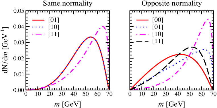
Figure 2: The normalized invariant $V$ mass distribution in the same normality case (Left) and in the opposite normality case (Right). Depending on the spin values and normalities of two particles, $X_{2}$ and $X_{1}$, the distribution shows its characteristic threshold behavior near the invariant-mass end point of $m=m_{2}-m_{1}=70\,{\rm GeV}$ for $m_{2}=100\,{\rm GeV}$ and $m_{1}=30\,{\rm GeV}$.

Consistently with the threshold behaviors listed in the last column of Table 2, the same-normality $[11]$ and opposite-normality $[01]$ and $[10]$ invariant-mass spectra decreases linearly with $\kappa_{*}\sim[(m_{2}-m_{1})-m]^{1/2}$ and therefore steeply just below the threshold, while the same-normality $[01]$ and $[10]$ and opposite-normality $[00]$ and $[11]$ invariant mass spectra decrease in a cubic power of $\kappa_{*}$ with $\kappa^{3}_{*}\sim[(m_{2}-m_{1})-m]^{3/2}$ and therefore rather gently as shown clearly in Figure 2. Even with this distinct threshold pattern, it is not possible to completely disentangle each spin-combination and normality case, as the normalized same-normality $[01]$ and $[10]$ spectra are identical. Therefore, it is necessary to utilize new independent observables for a more clear disentanglement.

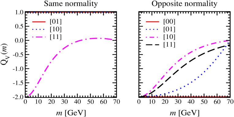
Figure 3: The tensor polarization ${\cal Q}_{V}(m)$ as a function of the invariant $V$ mass $m$ in the same normality case (Left) and in the opposite normality case (Right). Depending on the spin values and normalities of two particles, $X_{2}$ and $X_{1}$, the distribution shows its characteristic $m$ dependence. In this numerical analysis, $m_{2}=100\,{\rm GeV}$ and $m_{1}=30\,{\rm GeV}$ are taken.

In addition to the invariant-mass spectra, the tensor polarization ${\cal Q}_{V}(m)$ weighing the normalized correlated polar-angle distributions as shown in Eq. (60) provides us with an additional handle for identifying the spin combination and relative normalities. Figure 3 shows the dependence of the tensor polarization ${\cal Q}_{V}(m)$ on the invariant mass $m$. In the same-normality case, the $[11]$ polar-angle distribution can be clearly distinguished from the $[01]$ and $[10]$ polar-angle distributions, that are identical and constant, as a consequence of the fact that the reduced helicity amplitudes ${\cal C}_{0,0}$ are vanishing. In the opposite normality case, all the four spin-combination cases show different $m$-dependent behaviors. Specifically, ${\cal Q}_{V}(m)=-2$ in the $[00]$ case as only the longitudinal $V$ boson is produced. Consequently, we find that, although not perfect, the invariant-mass threshold behaviors and correlated polar-angle distributions enhance the resolution power for probing the spin and dynamical properties of the particles $X_{2}$ and $X_{1}$.

Tensor Polarization	Same normality				Opposite normality
$[s_{2}\,\,s_{1}]$	$[0\,0]$	$[0\,1]$	$[1\,0]$	$[1\,1]$	$[0\,0]$	$[0\,1]$	$[1\,0]$	$[1\,1]$
${\cal Q}_{V}(m_{V})$	–	$1.00$	$1.00$	$-0.32$	$-2.00$	$-1.66$	$-0.70$	$-1.08$

Table 2: The tensor polarization ${\cal Q}_{V}(m_{V})$ for $m_{2}=300\,{\rm GeV}$, $m_{1}=100\,{\rm GeV}$ and $m_{V}=m_{Z}=91.2\,{\rm GeV}$ for the combinations of the $X_{2}$ and $X_{1}$ spins, $s_{2}$ and $s_{1}$, in the same normality case and in the opposite normality case, respectively.

If the mass difference $m_{2}-m_{1}$ is larger than the $V$ mass $m_{V}$, then the vector boson $V$ is produced dominantly on-shell. In this situation, the invariant-mass distribution is not available any more. Nevertheless, the normalized correlated polar-angle distributions enable us to disentangle the spin and normality combinations at least partially, as shown in Table 2.

As can be checked in Eq. (60), the dependence of the correlated polar-angle correlations on the polar-angle $\theta$ of the particle $V$ is encoded in the first and second Legendre polynomials, $P_{1}(\cos\omega)=\cos\omega$ and/or $P_{2}(\cos\omega)=(3\cos^{2}\omega-1)/2$, because the Wick helicity rotation angle $\omega$ is a function of the polar angle $\theta$ as shown in Eqs. (46) and (47). Furthermore, they depend on the boost factor $\gamma_{2}=E_{2}/m_{2}$ denoting the energy $E_{2}$ of the decaying particle $X_{2}$ normalized to its mass $m_{2}$ in the LAB. As mentioned before, the longitudinal polarization ${\cal P}_{V}(m)$ is zero due to CPT invariance in the absence of absorptive parts. Therefore, the sensitivity of the polar-angle distribution to each spin and normality scenario is determined not only by the tensor polarization but also by the second Legendre polynomial.

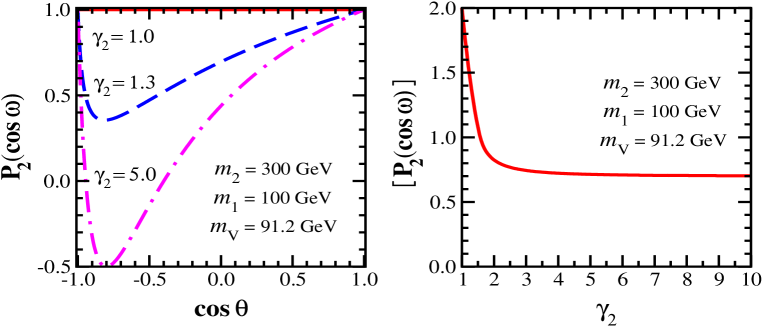
Figure 4: (Left) The behavior of the second Legendre polynomial $P_{2}(\cos\omega)=(3\cos^{2}\omega-1)/2$ of the Wick helicity rotation angle $\omega$ as a function of $\cos\theta$ for three values of the $X_{2}$ boost factor, $\gamma_{2}=1,1.3$ and $5$, corresponding to the $X_{2}$ speed, $\beta_{2}=0$, $\beta_{2}<\beta$ and $\beta_{2}>\beta$, respectively. (Right) The $\gamma_{2}$ dependence of the integral $[P_{2}(\cos\omega)]=\int^{1}_{-1}P_{2}(\cos\omega)\,d\cos\theta$. Numerically, $\beta\simeq 0.78$ for $m_{2}=300\,{\rm GeV}$, $m_{1}=100\,{\rm GeV}$ and $m_{V}=m_{Z}=91.2\,{\rm GeV}$.

The left frame of Figure 4 shows the behavior of the second Legendre polynomial $P_{2}(\cos\omega)=(3\cos^{2}\omega-1)/2$ as an implicit function of $\cos\theta$ for three values of the $X_{2}$ boost factor, $\gamma_{2}=1$ (red solid line), $1.3$ (blue dashed line) and $5$ (magenta dot-dashed line), corresponding to the $X_{2}$ speed, $\beta_{2}=0$, $\beta_{2}<\beta$ and $\beta_{2}>\beta$, respectively, and the right frame of Figure 4 shows the $\gamma_{2}$ dependence of the integral $[P_{2}(\cos\omega)]=\int^{1}_{-1}P_{2}(\cos\omega)\,d\cos\theta$. Both of them are based on the scenario ${\cal S}$2 of $m_{2}=300\,{\rm GeV}$, $m_{1}=100\,{\rm GeV}$ and $m_{V}=m_{Z}=91.2\,{\rm GeV}$, in which $\beta\simeq 0.78$. The $\cos\theta$ distribution is greatly influenced by the value of $\gamma_{2}$, when $\beta_{2}$ is less than $\beta$. Actually, $\cos\omega=0$ at $\cos\theta=-\beta/\beta_{2}\simeq-\beta\sim-0.78$ for $\gamma_{2}=5$, minimizing the second Legendre polynomial as shown by the magenta dot-dashed line in the left frame. In contrast, the shape of the curve changes so little for larger $\gamma_{2}$, as the value of $\beta_{2}$ remains very close to unity. The single lepton polar-angle distribution can be obtained by integrating the second Legendre polynomial over the angle $\theta$, which is still $\gamma_{2}$ dependent. The right frame shows the monotonic decrease of the integral $[P_{2}(\cos\omega)]$ converging asymptotically to a specific value. Actually, the analytic expression of the asymptotic value for a given $\beta$ is given by [54]

$${\cal L}_{(}\beta)=\frac{1}{\beta^{2}}\left[\,6-4\beta^{2}-\frac{3(1-\beta^{2})}{\beta}\ln\left(\frac{1+\beta}{1-\beta}\right)\,\right]\,,$$ (65)

which is approximately $0.7$ for $\beta$ very close to 1 in the scenario ${\cal S}2$ as shown in the right frame of Figure 4.

To summarize, we have shown how the invariant-mass and/or correlated polar-angle distributions can be expressed analytically in a compact form by use of the Wick helicity rotation angle and polarization functions and how they can be exploited efficiently for probing the $X_{2}X_{1}V$ vertex structure. Our restricted analysis is expected to be extended straightforwardly to the much more general and sophisticated scenarios.

5 Conclusions

We have made a general and systematic study of the vector currents of an on-shell or off-shell vector boson coupled to two integer-spin particles, of which the masses and spins do not have to be identical. The general vertex derived in a manifestly covariant formulation is applicable independently of whether the particles are neutral or charged. As a special case, we have probed in detail the case when the two particles are Majorana bosons and then we have worked out explicitly the constraints on the vertex due to discrete spacetime symmetries and the Majorana condition valid for the Majorana bosons.

The general results obtained in a manifestly covariant form have been checked through the study of two-body decays $X_{2}\to VX_{1}$ of a heavier Majorana boson $X_{2}$ into a lighter Majorana boson $X_{1}$ and an on-shell or off-shell vector boson $V$ based on the helicity formalism complementary to the covariant formalism as demonstrated.

Considering two sequential 2-body decays, $X_{2}\to VX_{1}$ and $V\to\ell^{-}\ell^{+}$ with $\ell=e$ and $\mu$, we have investigated how the correlated polar-angle and/or invariant-mass distributions enable us to determine the spin and dynamical structure of the triple vertex fully. As a specific comparison, for all the combinations with the spin value up to 1, we have found numerically that combining the invariant-mass and polar-angle distributions allow us to characterize the spin combinations effectively, although not perfect.

Although the half-integer spin case has to be worked out as well, this general and model-independent study of the vector currents of two massive (Majorana) particles of different masses and arbitrary integer spins presented in the present work can be exploited for searching for new BSM physics by probing various SM and BSM processes. Definitely, this work can be expanded significantly for the general analysis of the triple vertex of three particles of arbitrary spin.

References

• [1] S. L. Glashow, “Partial Symmetries of Weak Interactions,” Nucl. Phys. 22 (1961), 579-588 doi:10.1016/0029-5582(61)90469-2.
• [2] S. Weinberg, “A Model of Leptons,” Phys. Rev. Lett. 19 (1967), 1264-1266 doi:10.1103/PhysRevLett.19.1264.
• [3] A. Salam, “Weak and Electromagnetic Interactions,” Conf. Proc. C 680519 (1968), 367-377 doi:10.1142/9789812795915_0034.
• [4] E. Majorana, “Teoria simmetrica dell’elettrone e del positrone,” Nuovo Cim. 14 (1937), 171-184 doi:10.1007/BF02961314.
• [5] P. A. M. Dirac, “The quantum theory of the electron,” Proc. Roy. Soc. Lond. A 117 (1928), 610-624 doi:10.1098/rspa.1928.0023.
• [6] G. Aad et al. [ATLAS], “Observation of a new particle in the search for the Standard Model Higgs boson with the ATLAS detector at the LHC,” Phys. Lett. B 716 (2012), 1-29 doi:10.1016/j.physletb.2012.08.020 [arXiv:1207.7214 [hep-ex]].
• [7] S. Chatrchyan et al. [CMS], “Observation of a New Boson at a Mass of 125 GeV with the CMS Experiment at the LHC,” Phys. Lett. B 716 (2012), 30-61 doi:10.1016/j.physletb.2012.08.021 [arXiv:1207.7235 [hep-ex]].
• [8] P. Langacker, “Grand Unified Theories and Proton Decay,” Phys. Rept. 72 (1981), 185 doi:10.1016/0370-1573(81)90059-4.
• [9] D. Croon, T. E. Gonzalo, L. Graf, N. Košnik and G. White, “GUT Physics in the era of the LHC,” Front. in Phys. 7 (2019), 76 doi:10.3389/fphy.2019.00076 [arXiv:1903.04977 [hep-ph]].
• [10] P. Fayet and S. Ferrara, “Supersymmetry,” Phys. Rept. 32 (1977), 249-334 doi:10.1016/0370-1573(77)90066-7.
• [11] H. P. Nilles, “Supersymmetry, Supergravity and Particle Physics,” Phys. Rept. 110 (1984), 1-162 doi:10.1016/0370-1573(84)90008-5.
• [12] H. E. Haber and G. L. Kane, “The Search for Supersymmetry: Probing Physics Beyond the Standard Model,” Phys. Rept. 117 (1985), 75-263 doi:10.1016/0370-1573(85)90051-1.
• [13] M. C. Gonzalez-Garcia and M. Maltoni, “Phenomenology with Massive Neutrinos,” Phys. Rept. 460 (2008), 1-129 doi:10.1016/j.physrep.2007.12.004 [arXiv:0704.1800 [hep-ph]].
• [14] S. R. Elliott and M. Franz, “Colloquium: Majorana Fermions in nuclear, particle and solid-state physics,” Rev. Mod. Phys. 87 (2015), 137 doi:10.1103/RevModPhys.87.137 [arXiv:1403.4976 [cond-mat.supr-con]].
• [15] F. Wilczek, “Majorana returns,” Nature Phys. 5 (2009), 614–618 (2009), doi.org/10.1038/nphys1380.
• [16] A. J. Leggett, “Majorana fermions in condensed-matter physics,” Int. J. Mod. Phys. B 30 (2016) no.19, 1630012 doi:10.1142/S0217979216300127.
• [17] J. Schechter and J. W. F. Valle, “Majorana Neutrinos and Magnetic Fields,” Phys. Rev. D 24 (1981), 1883-1889 [erratum: Phys. Rev. D 25 (1982), 283] doi:10.1103/PhysRevD.25.283.
• [18] L. F. Li and F. Wilczek, “Physical Processes Involving Majorana Neuntrinos,” Phys. Rev. D 25 (1982), 143 doi:10.1103/PhysRevD.25.143.
• [19] P. B. Pal and L. Wolfenstein, “Radiative Decays of Massive Neutrinos,” Phys. Rev. D 25 (1982), 766 doi:10.1103/PhysRevD.25.766.
• [20] A. Halprin, S. T. Petcov and S. P. Rosen, “Effects of Light and Heavy Majorana Neutrinos in Neutrinoless Double Beta Decay,” Phys. Lett. B 125 (1983), 335-338 doi:10.1016/0370-2693(83)91296-0.
• [21] J. F. Nieves, “Two Photon Decays of Heavy Neutrinos,” Phys. Rev. D 28 (1983), 1664 doi:10.1103/PhysRevD.28.1664.
• [22] A. Khare and J. Oliensis, “Constraints on the Interactions of Majorana Particles From {CPT} Invariance,” Phys. Rev. D 29 (1984), 1542 doi:10.1103/PhysRevD.29.1542.
• [23] S. M. Bilenky, N. P. Nedelcheva and S. T. Petcov, “Some Implications of the {CP} Invariance for Mixing of Majorana Neutrinos,” Nucl. Phys. B 247 (1984), 61-69 doi:10.1016/0550-3213(84)90372-9.
• [24] S. P. Rosen, “General {CP} Properties of Neutrino Mass Eigenstates,” [erratum: Phys. Rev. D 30 (1984), 1995] doi:10.1103/PhysRevD.29.2535.
• [25] B. Kayser, “Majorana Neutrinos and their Electromagnetic Properties,” Phys. Rev. D 26 (1982), 1662 doi:10.1103/PhysRevD.26.1662.
• [26] B. Kayser, “CPT, CP, and C Phases and their Effects in Majorana Particle Processes,” Phys. Rev. D 30 (1984), 1023 doi:10.1103/PhysRevD.30.1023.
• [27] J. F. Nieves and P. B. Pal, “Electromagnetic properties of neutral and charged spin 1 particles,” Phys. Rev. D 55 (1997), 3118-3130 doi:10.1103/PhysRevD.55.3118 [arXiv:hep-ph/9611431 [hep-ph]].
• [28] J. F. Nieves, “Electromagnetic properties of spin-3/2 Majorana particles,” Phys. Rev. D 88 (2013), 036006 doi:10.1103/PhysRevD.88.036006 [arXiv:1308.5889 [hep-ph]].
• [29] E. E. Radescu, “Comments on the Electromagnetic Properties of Majorana Fermions,” Phys. Rev. D 32 (1985), 1266 doi:10.1103/PhysRevD.32.1266.
• [30] F. Boudjema, C. Hamzaoui, V. Rahal and H. C. Ren, “Electromagnetic Properties of Generalized Majorana Particles,” Phys. Rev. Lett. 62 (1989), 852 doi:10.1103/PhysRevLett.62.852.
• [31] F. Boudjema and C. Hamzaoui, “Massive and massless Majorana particles of arbitrary spin: Covariant gauge couplings and production properties,” Phys. Rev. D 43 (1991), 3748-3758 doi:10.1103/PhysRevD.43.3748.
• [32] J. R. Ellis, J. M. Frere, J. S. Hagelin, G. L. Kane and S. T. Petcov, “Search for Neutral Gauge Fermions in $e^{+}e^{-}$ Annihilation,” Phys. Lett. B 132 (1983), 436-442 doi:10.1016/0370-2693(83)90343-X.
• [33] S. T. Petcov, “Possible Signature for Production of Majorana Particles in $e^{+}e^{-}$ and $p\bar{p}$ Collisions,” Phys. Lett. B 139 (1984), 421-426 doi:10.1016/0370-2693(84)91844-6.
• [34] S. M. Bilenky, N. P. Nedelcheva and E. K. Khristova, “On Production of Majorana Particles in Polarized $e^{+}e^{-}$ Collisions,” Phys. Lett. B 161 (1985), 397-399 doi:10.1016/0370-2693(85)90786-5.
• [35] S. M. Bilenky, E. K. Khristova and N. P. Nedelcheva, “Possible Tests for Majorana Nature of Heavy Neutral Fermions Produced in Polarized $e^{+}e^{-}$ Collisions,” Bulg. J. Phys. 13 (1986), 283 JINR-E2-86-353.
• [36] S. T. Petcov, “{CP} Violation Effect in Neutralino Pair Production in $e^{+}e^{-}$ Annihilation and the Electric Dipole Moment of the Electron,” Phys. Lett. B 178 (1986), 57-64 doi:10.1016/0370-2693(86)90469-7.
• [37] G. A. Moortgat-Pick and H. Fraas, “Influence of CP and CPT on production and decay of Dirac and Majorana fermions,” Eur. Phys. J. C 25 (2002), 189-197 doi:10.1007/s10052-002-0979-x [arXiv:hep-ph/0204333 [hep-ph]].
• [38] E. K. Khristova and N. P. Nedelcheva, “On the Lightest Supersymmetric Particle in Polarized $e^{+}e^{-}$ Collisions,” Phys. Lett. B 208 (1988), 525-529 doi:10.1016/0370-2693(88)90661-2.
• [39] A. B. Balantekin, A. de Gouvêa and B. Kayser, “Addressing the Majorana vs. Dirac Question with Neutrino Decays,” Phys. Lett. B 789 (2019), 488-495 doi:10.1016/j.physletb.2018.11.068 [arXiv:1808.10518 [hep-ph]].
• [40] F. M. Renard, “Tests of Neutral Gauge Boson Self Couplings with $e^{+}e^{-}\to\gamma Z$,” Nucl. Phys. B 196 (1982), 93-108 doi:10.1016/0550-3213(82)90304-2.
• [41] K. Hagiwara, R. D. Peccei, D. Zeppenfeld and K. Hikasa, “Probing the Weak Boson Sector in $e^{+}e^{-}\to W^{+}W^{-}$,” Nucl. Phys. B 282 (1987), 253-307 doi:10.1016/0550-3213(87)90685-7.
• [42] D. Choudhury and S. D. Rindani, “Test of CP violating neutral gauge boson vertices in $e^{+}e^{-}\to\gamma Z$,” Phys. Lett. B 335 (1994), 198-204 doi:10.1016/0370-2693(94)91413-3 [arXiv:hep-ph/9405242 [hep-ph]].
• [43] B. Ananthanarayan, S. D. Rindani, R. K. Singh and A. Bartl, “Transverse beam polarization and CP-violating triple-gauge-boson couplings in $e^{+}e^{-}\to\gamma Z$,” Phys. Lett. B 593 (2004), 95-104 [erratum: Phys. Lett. B 608 (2005), 274-275] doi:10.1016/j.physletb.2005.01.009 [arXiv:hep-ph/0404106 [hep-ph]].
• [44] R. Rahaman and R. K. Singh, “On polarization parameters of spin-1 particles and anomalous couplings in $e^{+}e^{-}\rightarrow ZZ/Z\gamma$,” Eur. Phys. J. C 76 (2016) no.10, 539 doi:10.1140/epjc/s10052-016-4374-4 [arXiv:1604.06677 [hep-ph]].
• [45] R. Rahaman and R. K. Singh, “On the choice of beam polarization in $e^{+}e^{-}\rightarrow ZZ/Z\gamma$ and anomalous triple gauge-boson couplings,” Eur. Phys. J. C 77 (2017) no.8, 521 doi:10.1140/epjc/s10052-017-5093-1 [arXiv:1703.06437 [hep-ph]].
• [46] R. Rahaman, “Study of anomalous gauge boson self-couplings and the role of spin-$1$ polarizations,” [arXiv:2007.07649 [hep-ph]].
• [47] R. Rahaman and R. K. Singh, “Anomalous triple gauge boson couplings in $ZZ$ production at the LHC and the role of $Z$ boson polarizations,” Nucl. Phys. B 948 (2019), 114754 doi:10.1016/j.nuclphysb.2019.114754 [arXiv:1810.11657 [hep-ph]].
• [48] S. Y. Choi, T. Han, J. Kalinowski, K. Rolbiecki and X. Wang, “Characterizing invisible electroweak particles through single-photon processes at high energy $e^{+}e^{-}$ colliders,” Phys. Rev. D 92 (2015) no.9, 095006 doi:10.1103/PhysRevD.92.095006 [arXiv:1503.08538 [hep-ph]].
• [49] S. Y. Choi, J. Kalinowski, G. A. Moortgat-Pick and P. M. Zerwas, “Analysis of the neutralino system in supersymmetric theories,” Eur. Phys. J. C 22 (2001), 563-579 doi:10.1007/s100520100808 [arXiv:hep-ph/0108117 [hep-ph]].
• [50] S. Y. Choi, “Probing the weak boson sector in $\gamma e\to Ze$,” Z. Phys. C 68 (1995), 163-172 doi:10.1007/BF01579815 [arXiv:hep-ph/9412300 [hep-ph]].
• [51] S. Y. Choi and Y. G. Kim, “Analysis of the neutralino system in two body decays of neutralinos,” Phys. Rev. D 69 (2004), 015011 doi:10.1103/PhysRevD.69.015011 [arXiv:hep-ph/0311037 [hep-ph]].
• [52] S. Y. Choi, B. C. Chung, J. Kalinowski, Y. G. Kim and K. Rolbiecki, “Analysis of the neutralino system in three-body leptonic decays of neutralinos,” Eur. Phys. J. C 46 (2006), 511-520 doi:10.1140/epjc/s2006-02482-1 [arXiv:hep-ph/0504122 [hep-ph]].
• [53] S. Y. Choi, “$Z$-boson polarization as a model-discrimination analyzer,” Phys. Rev. D 98 (2018) no.11, 115037 doi:10.1103/PhysRevD.98.115037 [arXiv:1811.10377 [hep-ph]].
• [54] S. Y. Choi, J. H. Jeong and J. H. Song, “General Spin Analysis from Angular Correlations in Two-Body Decays,” Eur. Phys. J. Plus 135 (2020) no.2, 210 doi:10.1140/epjp/s13360-020-00132-1 [arXiv:1903.00166 [hep-ph]].
• [55] S. Y. Choi and J. H. Jeong, “A Nondiagonal Pair of Majorana Particles at $e^{+}e^{-}$ Colliders,” [arXiv:2012.14613 [hep-ph]].
• [56] M. Jacob and G. C. Wick, “On the General Theory of Collisions for Particles with Spin,” Annals Phys. 7 (1959), 404-428 doi:10.1016/0003-4916(59)90051-X.
• [57] G. C. Wick, “Angular momentum states for three relativistic particles,” Annals Phys. 18 (1962), 65-80 doi:10.1016/0003-4916(62)90059-3.
• [58] E. Leader, “Spin in particle physics,” Camb. Monogr. Part. Phys. Nucl. Phys. Cosmol. 15 (2011), pp.1-500.
• [59] S. U. Chung, “SPIN FORMALISMS,” doi:10.5170/CERN-1971-008.
• [60] R. E. Behrends and C. Fronsdal, “Fermi Decay of Higher Spin Particles,” Phys. Rev. 106 (1957) no.2, 345 doi:10.1103/PhysRev.106.345.
• [61] P. R. Auvil and J. J. Brehm, “Wave Functions for Particles of Higher Spin,” Phys. Rev. 145 (1966) no.4, 1152 doi:10.1103/PhysRev.145.1152.
• [62] S. Weinberg, “The Quantum theory of fields. Vol. 1: Foundations,” (Cambridge University Press, 1995), ISBN 0-521-55001-7.
• [63] L. D. Landau, “On the angular momentum of a system of two photons,” Dokl. Akad. Nauk SSSR 60 (1948) no.2, 207-209 doi:10.1016/B978-0-08-010586-4.50070-5.
• [64] C. N. Yang, “Selection Rules for the Dematerialization of a Particle Into Two Photons,” Phys. Rev. 77 (1950), 242-245 doi:10.1103/PhysRev.77.242.
• [65] M. E. Rose, “Elementary Theory of Angular Momentum” (Dover Publication Inc., New York, 2011) ISBN-13: 978-0486684802.
• [66] P. A. Zyla et al. [Particle Data Group], “Review of Particle Physics,” PTEP 2020 (2020) no.8, 083C01 doi:10.1093/ptep/ptaa104.
• [67] J. M. Cornwall, D. N. Levin and G. Tiktopoulos, “Derivation of Gauge Invariance from High-Energy Unitarity Bounds on the s Matrix,” Phys. Rev. D 10 (1974), 1145 [erratum: Phys. Rev. D 11 (1975), 972] doi:10.1103/PhysRevD.10.1145.
• [68] C. E. Vayonakis, “Born Helicity Amplitudes and Cross-Sections in Nonabelian Gauge Theories,” Lett. Nuovo Cim. 17 (1976), 383 doi:10.1007/BF02746538.
• [69] M. S. Chanowitz and M. K. Gaillard, “The TeV Physics of Strongly Interacting W’s and Z’s,” Nucl. Phys. B 261 (1985), 379-431 doi:10.1016/0550-3213(85)90580-2.
• [70] S. U. Chung, “Helicity coupling amplitudes in tensor formalism,” Phys. Rev. D 48 (1993), 1225-1239 [erratum: Phys. Rev. D 56 (1997), 4419] doi:10.1103/PhysRevD.56.4419.
• [71] S. U. Chung, “A General formulation of covariant helicity coupling amplitudes,” Phys. Rev. D 57 (1998), 431-442 doi:10.1103/PhysRevD.57.431.
• [72] S. U. Chung, “Covariant helicity-coupling amplitudes: Principles and examples,” Int. J. Mod. Phys. A 18 (2003), 457-473 doi:10.1142/S0217751X03014381.
• [73] S. U. Chung and J. Friedrich, “Covariant helicity-coupling amplitudes: A New formulation,” Phys. Rev. D 78 (2008), 074027 doi:10.1103/PhysRevD.78.074027 [arXiv:0711.3143 [hep-ph]].