Space charge fields in azimuthally symmetric beams: integrated Green’s function approach

Abstract

Electromagnetic fields induced by the space charge in relativistic beams play an important role in Accelerator Physics. They lead to emittance growth, slice energy change, and the microbunching instability. Typically, these effects are modeled numerically since simple description exists only in the limits of large- or small-scale current variations. In this paper we consider an axially symmetric charged beam inside a round pipe and find the solution of the space charge problem that is valid in the full range of current variations. We express the solution for the field components in terms of Green’s functions, which are fully determined by just a single function. We then find that this function is an on-axis potential from a charged disk in a round pipe, with transverse charge density $\rho_{\perp}(r)$, and it has a compact analythical expression. We finally provide an integrated Green’s function based approach for efficient numerical evaluation in the case when the transverse charge density stays the same along the beam.

I Introduction

The space charge effect is a basic collective phenomenon in Accelerator Physics that plays an important role both in electron and proton machines. In high current regimes, self-generated electromagnetic fields become so strong that they lead to significant emittance growth a:Chasman:1969 ; a:Lapostolle:1971 ; a:Hofmann:1981 ; a:Kim:1989 , slice energy change, and the microbunching instability a:Huang:2004 , which is especially detrimental in the context of free electron laser linacs a:Borland:2002 ; a:Huang:2004 . In the case of x-ray free electron lasers with periodic enhancement of electron peak current a:Zholents:2005 ; a:Kur:2011 ; a:Tanaka:2013 , strong longitudinal current modulation may result in large space charge forces which, in turn, may limit the performance of these schemes.

Compact analytical expressions for the space charge induced fields are currently available in the limits of either large- or small-scale current variations. The first limit provides a local description b:Chao:1993 while the second limit requires an impedance based description tr:Rosenzweig:1996 that is non-local as it depends on the Fourier spectrum of the current. This latter approach allows for semi-analytical treatment and is implemented in the Elegant numerical code tr:Borland:2000 in order to include longitudinal space charge effects on a beam axis.

An alternative approach adopted in many numerical codes, such as OPAL tr:OPAL:2008 , Astra web:Floettmann:2011 , and Parmela tr:Billen:1996 . This approach uses a Poison solver in order to find the space charge induced fields. However it is very time consuming and a semi-analytic description for the space charge induced fields applicable in the full range of current variations is highly desired.

In this paper we provide a semi-analytical description of the space charge problem in the case of an axially symmetric beam in a round pipe. The derived expressions for components of the induced field are valid in the full range of current variations. They also can be efficiently evaluated by the method of Integrated Green’s functions (IGF).

We present our approach in Section II, where we find that the Green’s function for a charged disk in a round pipe fully determines the components of the induced fields. In Section III, we express the Green’s function in terms of an on-axis potential from a charged disk in a round pipe and find a compact analytical approximation for this potential. Section IV uses the compact analytical expression for the Green’s function in order to present the field components in a form suitable for the IGF approach. In Section V we suggest how to improve a semi-analytical description of the space charge fields in numerical codes such as Elegant by providing a step-by-step instructions of IGF approach with our Green’s function. We finally summarize our findings in the conclusion.

II Basic Equations for the Space Charge Fields

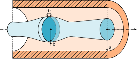
Figure 1: An axially symmetric electron beam in a perfectly conducting pipe of radius $a$. A disk section of length $dz$ and the transverese charge density $\rho_{\perp}\left(r,z\right)$, where $z$ is a coordinate along the beam in the beam reference frame, is shown.

The most general approach considers an electron beam with charge density $\rho(\mathbf{r})$ that travels on axis of a perfectly conducting pipe of radius $a$ at a speed $v_{z}$ (see Fig. 1). It starts in the beam frame, $\mathbf{R}$, where the electrostatic potential induced by the space charge, $\varrho(\mathbf{R})$, is a solution of the Poisson equation:

$$\Phi(\mathbf{R})=\frac{1}{4\pi\varepsilon_{0}}\int\varrho(\mathbf{R^{\prime}})\Gamma(\mathbf{R}|\mathbf{R^{\prime}})d^{3}\mathbf{R^{\prime}},$$ (1)

where $\Gamma(\mathbf{R}|\mathbf{R^{\prime}})$ is the Green’s function for the Laplace’s equation inside a perfectly conducting pipe. The corresponding Green’s function is derived in Appendix as an expansion in terms of radial-azimuthal eignenfunctions that can be used in systems without translational symmetry.

In this paper, we will consider axially symmetric densities in the lab frame, $\mathbf{r}$, of the form $\rho(\mathbf{r})=\rho_{\perp}(r)\lambda(z)$ with normalization $\int\rho_{\perp}(r^{\prime})d^{2}\mathbf{r^{\prime}}=1$. In this case, the electrostatic potential in the beam frame is expressed as

$$\Phi(R,Z)=\frac{1}{4\pi\varepsilon_{0}}\int_{-\infty}^{\infty}\Lambda(Z^{\prime})G(R,Z-Z^{\prime})dZ^{\prime},$$ (2)

where $\Lambda(Z^{\prime})=\gamma^{-1}\lambda(Z^{\prime}/\gamma)$ and

$$G(R,Z-Z^{\prime})=\sum_{n=1}^{\infty}\frac{2c_{n}J_{0}(\mu_{0,n}R/a)}{a\mu_{0,n}J_{1}(\mu_{0,n})^{2}}e^{-\mu_{0,n}|Z-Z^{\prime}|/a},$$ (3)

with $c_{n}=\int\rho_{\perp}(r^{\prime})J_{0}(\mu_{0,n}r^{\prime}/a)d^{2}\mathbf{r^{\prime}}$ that has to be individually calculated for different transverse density profiles. In the particular case of $c_{n}=1$, one recovers a result for an electrostatic potential of a point charge on the axis of a perfectly conducting pipe (see Eq. (27) in Ref. a:Bouwkamp:1947 ).

The electrostatic potential in the beam reference frame results in the electric field with longitudinal and transverse components that have the following expressions in the lab frame

$$E_{z}(r,z)=-\frac{1}{4\pi\varepsilon_{0}\gamma}\int_{-\infty}^{\infty}\lambda(z^{\prime})\frac{\partial}{\partial z}g(r,z-z^{\prime})dz^{\prime},$$ (4)

$$E_{r}(r,z)=-\frac{\gamma}{4\pi\varepsilon_{0}}\int_{-\infty}^{\infty}\lambda(z^{\prime})\frac{\partial}{\partial r}g(r,z-z^{\prime})dz^{\prime},$$ (5)

in terms of transformed to the lab frame Green’s function, $g(r,z-z^{\prime})=G(r,\gamma z-\gamma z^{\prime})$. Additionally, in the lab frame, there is also an azimuthal magnetic field $B_{\phi}(r,z)=\frac{v_{z}}{c^{2}}E_{r}(r,z)$, which reduces the overall transverse space charge force acting on charged particles in the beam by $\gamma^{-2}$.

III Green’s function analysis

In the previous section, we have reduced the problem of space charge induced fields to the finding Green’s function, $G(R,Z-Z^{\prime})$, — the electrostatic potential from a charge distribution, $\varrho(\mathbf{R})=\rho_{\perp}(R)\delta(Z-Z^{\prime})$. Due to the axial symmetry of the charge distribution, one can use the Poisson representation a:Poisson:1823 in order to the potential outside the axis of symmetry once the potential on the axis has been found:

$$G(R,Z-Z^{\prime})=\frac{1}{2\pi}\int_{0}^{2\pi}G(0,Z-Z^{\prime}+iR\cos\phi)d\phi,\ Z>Z^{\prime},$$ (6)

where

$$G(0,Z-Z^{\prime})=\sum_{n=1}^{\infty}\frac{2c_{n}}{a\mu_{0,n}J_{1}(\mu_{0,n})^{2}}e^{-\mu_{0,n}|Z-Z^{\prime}|/a}.$$ (7)

Sometimes, however, the integral cannot be taken analytically or potential has to be found near the axis. Therefore, we propose an alternative approach here based on the formal separation of variables:

$$G(R,Z-Z^{\prime})\equiv J_{0}\left(R\frac{\partial}{\partial Z}\right)G(0,Z-Z^{\prime}),\ Z\neq Z^{\prime},$$ (8)

where a function of a derivative is defined via its Taylor series expansion . As a consequence of our approach, one can confirm, based on a formal substitution $x\to R\frac{\partial}{\partial Z}$ into the Bessel differential equation, $\left(x^{2}\frac{d^{2}}{dx^{2}}+x\frac{d}{dx}+x^{2}\right)J_{0}\left(x\right)=0$, that the derived Green’s function is indeed a solution of the Laplace equation, $\left(\frac{\partial^{2}}{\partial R^{2}}+\frac{1}{R}\frac{\partial}{\partial R}+\frac{\partial^{2}}{\partial Z^{2}}\right)G(R,Z-Z^{\prime})=0$.

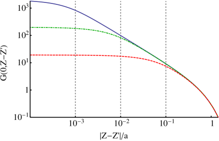
Figure 2: (Color online) An on-axis Green’s function, $G(0,Z-Z^{\prime})$, in case of uniform transverse distribution for different values of $b/a=$ 0.1 (dashed red), 0.01 (dot dashed green) and 0.001 (solid blue). The short-range behavior, $|Z-Z^{\prime}|\ll a$, corresponds to the potential from a uniformly charged disk of radius $b$ in free space. As distance increases, $|Z-Z^{\prime}|\gg b$, the on-axis Green’s function becomes the potential of a point charge in a pipe. Transformation to the lab frame substitutes $Z\to\gamma z$ thus scaling the transitions points to $a/\gamma$ and $b/\gamma$ correspondingly.

As the transformed Green’s function is $g(r,z-z^{\prime})=G(r,\gamma z-\gamma z^{\prime})$, we have just reduced the space charge problem to finding electrostatic potential on the pipe axis, $G(0,Z-Z^{\prime})$, which is shown in Fig. 2, in the case of a uniform transverse distribution, $\rho_{\perp}(r<b)=1/\pi b^{2}$, for different values of $b/a$. It shows that there are two distinct regions with different behaviors of the Green’s function. The first region corresponds to the far zone, $|Z-Z^{\prime}|\gg b$, where the Green’s function is just a potential of a point charge in a pipe. The second region corresponds to the vicinity of the source, $|Z-Z^{\prime}|\ll a$, in which case the free space approximation can be used. Both of these regions allow for accurate and compact analytical expressions for $G(0,Z-Z^{\prime})$. Furthermore, we can be combined these expressions together in a single analytical expression due to a broad overlap region, $b\ll|Z-Z^{\prime}|\ll a$, which corresponds to a point charge in a free space.

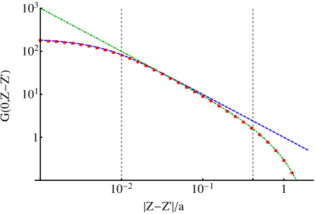
Figure 3: (Color online) The on-axis Green’s function, $G(0,z-z^{\prime})$ in the case of uniform transverse charge density with $b/a=0.01$ (red squares). The near (dashed blue) and far (dot-dashed green) zone contributions are plotted separately. The boundaries of these zones $|Z-Z^{\prime}|=\mu_{0,1}^{-1}a$ and $|Z-Z^{\prime}|=b$ are marked by the vertical dashed lines. Transformation to the lab frame substitutes $Z\to\gamma z$ thus scaling the transitions points to $\mu_{0,1}^{-1}a/\gamma$ and $b/\gamma$ correspondingly.

In the first region, $|Z-Z^{\prime}|\gg b$, the sum in Eq. (7) converges rapidly due to vanishing exponential factors $\exp(-\mu_{0,n}|Z-Z^{\prime}|/a)$. The actual number of terms contributing to the sum can be estimated as $\mu_{0,n}|Z-Z^{\prime}|/a\sim 1$. Under this condition, $c_{n}\simeq 1$, resulting in the expression for the on-axis potential from a point charge on the pipe axis a:Bouwkamp:1947 . A compact form representation for the on-axis Green’s function in the far zone is hence a sum of the geometric series:

$$G(0,Z-Z^{\prime})\approx\frac{1}{a}\frac{\pi e^{-\mu_{0,1}|Z-Z^{\prime}|/a}}{1-e^{-\pi|Z-Z^{\prime}|/a}},\ |Z-Z^{\prime}|\gg b,$$ (9)

where we have used that $\mu_{0,n}-\mu_{0,1}\approx\pi(n-1)$ and $\mu_{0,n}J_{1}(\mu_{0,n})^{2}\approx 2/\pi$.

The second region is in the vicinity of the source, $|Z-Z^{\prime}|\ll a$. Hence, one can ignore a boundary effect of the pipe surface but has to account for an actual transverse charge density, $\rho_{\perp}(r)$. In the absence of the boundary effect the convergence of the sum in Eq. (7) is defined by $c_{n}$ rather than by the exponent. Hence, one can replace summation with integration. We chose the integration variable to be $x=\mu_{0,n}$ with the Jacobian of this transformation $dn/dx\simeq 1/\pi$:

$$G(0,Z-Z^{\prime})\approx\frac{1}{a}\int d^{2}\mathbf{r^{\prime}}\rho_{\perp}(r^{\prime})\int_{0}^{\infty}J_{0}(xr^{\prime}/a)e^{-x|Z-Z^{\prime}|/a}dx.$$ (10)

Carrying out one integration results in the following compact form representation of the on-axis Green’s function

$$G(0,Z-Z^{\prime})\approx\int d^{2}\mathbf{r^{\prime}}\frac{\rho_{\perp}(r^{\prime})}{\sqrt{(Z-Z^{\prime})^{2}+r^{\prime 2}}},\ |Z-Z^{\prime}|\ll a,$$ (11)

which is indeed the on-axis potential from a charged disk in free space. The Table 1 provides examples of this potential for different transverse charge distributions.

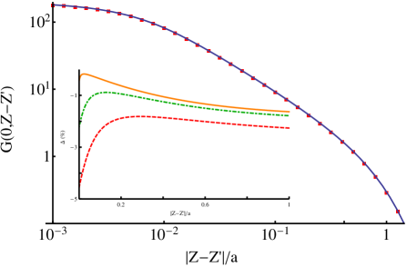
Figure 4: (Color online) The on-axis Green’s function, red squares, and its analythical approximation, blue line, for the uniform transverse charge density with $b/a=0.01$. The inset shows the relative error, $\Delta$, between the exact and analytical representations of the on-axis response function. The red dashed line corresponds to $b/a=0.1$, while the green dot-dashed and solid orange lines correspond to $b/a=0.05$ and $b/a=0.01$ respectively.

So far, we have found two analytical representations for the on-axis Green’s function that describe two physical limits. Figure 3 compares these approximate representations given by Eqs. (9) and (11) with values of the on-axis Green’s function given in Eq. (7). It shows that approximate expressions describe the on-axis Green’s function well within their applicability regions. We note that there is an overlap region where two physical limits have common domain of mutual applicability, $b\ll|Z-Z^{\prime}|\ll a$. This region is well defined when the beam size is sufficiently smaller than the pipe radius, $b<a$, and correspond to the case where the charge distribution can be already approximated by a point charge yet the presence of pipe walls can be still ignored. In this region, both expressions result in the same asymptotic form for the on-axis Green’s function and coincide with the expression for the point charge potential in free space:

$$G(0,Z-Z^{\prime})=\frac{1}{|Z-Z^{\prime}|},\ b\ll|Z-Z^{\prime}|\ll a.$$ (12)

This allows matching of the two analytical representations as their product divided by their mutual asymptotic expression. As a result, the on-axis Green’s function in a perfectly conducting pipe can be approximated with:

$$G(0,Z-Z^{\prime})\approx\frac{|Z-Z^{\prime}|}{a}\frac{\pi e^{-\mu_{0,1}|Z-Z^{\prime}|/a}}{1-e^{-\pi|Z-Z^{\prime}|/a}}\int d^{2}\mathbf{r^{\prime}}\frac{\rho_{\perp}(r^{\prime})}{\sqrt{(Z-Z^{\prime})^{2}+r^{\prime 2}}},$$ (13)

for $b<a$ and $|Z-Z^{\prime}|\in(0,\infty)$.

$\rho_{\perp}(r)$		$b$	$\int d^{2}\mathbf{r^{\prime}}\frac{\rho_{\perp}(r^{\prime})}{\sqrt{(Z-Z^{\prime})^{2}+r^{\prime 2}}}$
$\frac{1}{\pi b^{2}},$	$r\leq b$	$2x_{rms}$	$\frac{2}{b}\frac{1}{|\Delta Z|+\sqrt{\Delta Z^{2}+1}}$
$\frac{2}{\pi b^{2}}\left(1-\frac{r^{2}}{b^{2}}\right),$	$r\leq b$	$\sqrt{6}x_{rms}$	$\frac{8}{3b}\frac{1+3\Delta Z^{2}/4}{|\Delta Z|^{3}+\left(\Delta Z^{2}+1\right)^{3/2}+3|\Delta Z|/2}$
$\frac{1}{\pi b^{2}}e^{-r^{2}/b^{2}},$	$r\leq\infty$	$\sqrt{2}x_{rms}$	$\frac{\sqrt{\pi}}{b}Erfc\left(|\Delta Z|\right)e^{\Delta Z^{2}}$

Table 1: The transverse density distributions with their rms sizes and the corresponding on-axis Green’s functions in the vicinity of the sources with $\Delta Z=(Z-Z^{\prime})/b$.

The main advantage of using the compact form expression is its simplicity. In contrast, evaluation of an exact Green’s function described with Eq. (7) requires summation of a large number of terms and takes a significant amount of time. Figure 4 shows the comparison between these two approaches for the uniform transverse charge distribution with $b/a=0.01$. The inset shows the relative error of using the approximate Green’s function instead of exact. The absolute error is the largest at $Z=Z^{\prime}$ but does not exceed $0.87069/a$ based on a simple method of summing Bessel series proposed by Greenwood in Ref. a:Greenwood:1968 .

IV The Integrated Green’s Function Approach

In the previous section, we have provided a compact form for the Green’s function that describes an axially symmetric space charge problem. Using this result, the longitudinal space charge field takes on the following form for the translationally invariant transverse distributions

$$E_{z}(r,z)=\frac{1}{4\pi\varepsilon_{0}\gamma}\int_{-\infty}^{\infty}\lambda(z^{\prime})\frac{\partial}{\partial z^{\prime}}g_{z}(r,z-z^{\prime})dz^{\prime},$$ (14)

with $g_{z}(r,z-z^{\prime})=J_{0}\left(\frac{r}{\gamma}\frac{\partial}{\partial z}\right)g(0,z-z^{\prime})$. The operational form for the Green’s function suggested in Eq. 8 also allows for a similar representation for the transverse component of the space charge induced field

$$E_{r}(r,z)=\frac{1}{4\pi\varepsilon_{0}}\int_{-\infty}^{\infty}\lambda(z^{\prime})\frac{\partial}{\partial z^{\prime}}g_{r}(r,z-z^{\prime})dz^{\prime},$$ (15)

with $g_{r}(r,z-z^{\prime})=-J_{1}\left(\frac{r}{\gamma}\frac{\partial}{\partial z}\right)g(0,z-z^{\prime})$ . This solution for the space charge problem allows for efficient numerical evaluation based on the Integrated Green’s function approach ip:Ryne:2003 ; ip:Abell:2007 ; a:Qiang:2007 .

For the purposes of providing a recipe for numerical evaluation of the Eqs. 14 and 15, we will use the Integrated Green’s function approach in a constant function basis. This approach approximates the charge density as $\lambda(z^{\prime})=\left(\lambda_{j+1}+\lambda_{j}\right)/2$ within a cell of the computational domain, $z^{\prime}\in\left[z_{j},z_{j+1}\right]$ for $z_{j}=jh$, and arrives to the following discrete convolution

$$E_{r,z}(z_{i})=hA_{r,z}\sum_{j}\lambda_{j}w_{r,z}^{i-j},$$ (16)

with normalization constants $A_{r}=1/4\pi\varepsilon_{0}$ and $A_{z}=A_{r}/\gamma$.

The Green’s functions derived in this paper behave differently near the source. Namely, the longitudinal Green’s function, $g_{z}(r,z-z^{\prime})$, is a continuous function of $z$, while the radial Green’s function, $g_{r}(r,z-z^{\prime})$, has a discontinuity at $z=z^{\prime}$. Taking this into account, leads to the following integrated Green’s function for the longitudinal component

$$w_{z}(\zeta)=\frac{g_{z}(r,\zeta-h)-g_{z}(r,\zeta+h)}{2h},$$ (17)

with $\zeta=h(i-j)$; and for the radial component:

$$w_{r}(\zeta)=\frac{g_{r}(r,\zeta-h)-g_{r}(r,\zeta+h)}{2h}+\frac{1}{h}g_{r}(r,0^{-})\delta_{\zeta,(-h,0,h)},$$ (18)

where $w_{r}(h)$ uses the Green’s function defined for $z\geq z^{\prime}$ in order to evaluate $g_{r}(r,0)$, while $w_{r}(-h)$ and $g_{r}(r,0^{-})$ use $z\leq z^{\prime}$ definition.

V Discussion

Equation 13 is the main result of the paper that has allowed us to express the space charge induced fields in terms of the Green’s functions that have simple analythical representation. Equations 14 and 15 with the corresponding Green’s function are the next important result of this paper. These expressions for the components of the field can be efficiently evaluated using the Integrated Green’s functions, Eqs. 17 and 18.

It is often a case that the transverse beam size is a smallest scale of the problem and that only the space charge induced fields within the beam are of interest. Thus, the particle accelerator codes, similar to Elegant, include only the effects of the space charge induced fields at $r=0$. X-ray free electron lasers often operate in a space charge dominated regime and a more diligent treatment of the space charge induced fields is in order. In what follows we will illustrate the steps required to obtain the off-axis behavior for the components of the space charge induces field.

The radial component of the space charge induced field, evaluated on $z_{i}=ih$ grid, is equal to $E_{r}(z_{i})=hA_{r}\sum_{j}\lambda_{j}w_{r}^{i-j}$, where $\lambda_{j}$ is a space charge distribution on the same grid and $A_{r}=1/4\pi\varepsilon_{0}$. Equation 18 defines the integrated Green’s function, $w_{r}(\zeta)$, in terms of

$$g_{r}(r,z-z^{\prime})=-\frac{r}{2}\frac{\partial}{\gamma\partial z}g(0,z-z^{\prime}),$$ (19)

where we have kept the leading term in the Taylor series expansion of $J_{1}(x)$ for the purpose of illustration only. In order to evaluate the derivation of the on-axis Green’s function, we can apply the logic used in deriving the analythical representation of the on-axis Green’s function itself and arrive to the following expression:

$$\frac{\partial}{\partial Z}G(0,Z-Z^{\prime}) \approx \frac{|Z-Z^{\prime}|^{3}}{a}\left(\frac{\partial}{\partial Z}\frac{\pi e^{-\mu_{0,1}|Z-Z^{\prime}|/a}}{1-e^{-\pi|Z-Z^{\prime}|/a}}\right)\times$$ (20)

$$\times \int d^{2}\mathbf{r^{\prime}}\frac{\rho_{\perp}(r^{\prime})}{\left[(Z-Z^{\prime})^{2}+r^{\prime 2}\right]^{3/2}}.$$

Evaluation of the longitudinal component of the space charge induced field follows the same steps but uses $A_{z}=A_{r}/\gamma$ and $w_{z}(\zeta)$ as defined in Eq. 17 in terms of

$$g_{z}(r,z-z^{\prime})=\left(1-\frac{r^{2}}{4}\frac{\partial^{2}}{\gamma^{2}\partial z^{2}}\right)g(0,z-z^{\prime}),$$ (21)

where we have kept the first two leading terms in the Taylor series expansion of $J_{0}(x)$ for the purpose of illustration only. The second term requires the second derivative of the on-axis Green’s function that has the following form:

$$\frac{\partial^{2}}{\partial Z^{2}}G(0,Z-Z^{\prime}) \approx \frac{|Z-Z^{\prime}|^{3}}{2a}\left(\frac{\partial^{2}}{\partial Z^{2}}\frac{\pi e^{-\mu_{0,1}|Z-Z^{\prime}|/a}}{1-e^{-\pi|Z-Z^{\prime}|/a}}\right)\times$$ (22)

$$\times \int d^{2}\mathbf{r^{\prime}}\frac{\rho_{\perp}(r^{\prime})\left[2(Z-Z^{\prime})^{2}-r^{\prime 2}\right]}{\left[(Z-Z^{\prime})^{2}+r^{\prime 2}\right]^{5/2}}.$$

From the provided illustration, the solution of the space charge problem at $r=0$ requires a single evaluation of a discreet convolution. An additional convolution provides a linear contribution to the radial component of the space charge induced field. The third convolution can be also carried out in order to find a next order correction to the longitudinal component of the space charge induced field. One can apply the illustrated approach in order to find the next order corrections with computational effort that scales linearly with number of corrections.

VI Conclusions

We have studied the space charge problem for the beam with axially symmetric charge distribution in a smooth perfectly conducting pipe. We have develop a Green’s function-based description for the space charge induced fields that is valid in the full range of current variations and applicable to beams with varying beam radius. The Green’s function discussed in the paper corresponds to the electrostatic potential of a charged disk in a pipe and is completely defined by its behavior on the pipe axis due to axial symmetry.

We have found a compact analytical approximation for the on-axis Green’s function that allows for analytical calculation of the Green’s function off axis. Having a compact representation of the on-axis behavior of the response function can improve semi-analytical codes, such as Elegant, as it offers a significant advantage over numerical evaluation of the exact solution.

Finally, we have provided a detail prescription based on the Integrated Green’s function approach for efficient numerical evaluation of the fields in the case of translational symmetry. This approach describes transverse as well as longitudinal component of the space charge induced field and scales linearly with the number of radial corrections.

VII Acknowledgements

We gratefully acknowledge the support of the U.S. Department of Energy through the LANL/LDRD Program for this work.

Appendix A Green’s function

The Green’s function for the Laplace’s equation inside a perfectly conducting pipe must satisfy the following equation

$$\nabla^{2}\Gamma(\mathbf{R}|\mathbf{R^{\prime}})=-4\pi\delta(\mathbf{R}-\mathbf{R^{\prime}})$$ (23)

with the boundary condition $\Gamma(R=a)=0$ and $\Gamma(Z\to\pm\infty)=0$.

To find a Green’s function, it is common to expand the Green’s function in terms of axial eigenfunction solutions of the Laplace’s problem in cylindrical coordinates, $e^{ikZ}$. Here, however, the radial eigenfunction expansion is used in order to allow for beam size variation along the beam. Thus

$$\Gamma(\mathbf{R}|\mathbf{R^{\prime}})=\sum_{m=-\infty}^{\infty}\sum_{n=1}^{\infty}G_{m,n}(Z|\mathbf{R^{\prime}})J_{m}(\mu_{m,n}R/a)e^{im\Phi},$$ (24)

where $J_{m}$ is the ordinary Bessel’s function of order $m$ and $\mu_{m,n}$ is defined as a solution of $J_{m}\left(\mu_{m,n}\right)=0$. Substituting this expansion in 23 we find that

$$\nabla^{2}\Gamma(\mathbf{R}|\mathbf{R^{\prime}})=\sum_{m=-\infty}^{\infty}\sum_{n=1}^{\infty}\left[\frac{d^{2}G_{m,n}(Z|\mathbf{R^{\prime}})}{dZ^{2}}-\right.$$

$$\left.-\frac{\mu_{m,n}^{2}}{a^{2}}G_{m,n}(Z|\mathbf{R^{\prime}})\right]J_{m}(\mu_{m,n}R/a)e^{im\Phi}.$$ (25)

With the help of the orthogonality properties for the Bessel’s function, we can now obtain that

$$\frac{d^{2}G_{m,n}(Z|\mathbf{R^{\prime}})}{dZ^{2}}-\frac{\mu_{m,n}^{2}}{a^{2}}G_{m,n}(Z|\mathbf{R^{\prime}})=$$

$$-\frac{4}{a^{2}J_{m+1}(\mu_{m,n})^{2}}J_{m}(\mu_{m,n}R^{\prime}/a)e^{-im\Phi^{\prime}}\delta(Z-Z^{\prime}).$$ (26)

Then, if we look at the points where $z\neq z^{\prime}$, (A) becomes a simple eigen function problem with a well known solution

$$G_{m,n}(Z|\mathbf{R^{\prime}})=g_{m,n}(R^{\prime},\Phi^{\prime})e^{-\mu_{m,n}|Z-Z^{\prime}|/a}.$$ (27)

The condition for the discontinuity of the first derivative at $Z=Z^{\prime}$ yields that

$$g_{m,n}(R^{\prime},\Phi^{\prime})=\frac{2}{a\mu_{m,n}J_{m+1}(\mu_{m,n})^{2}}J_{m}(\mu_{m,n}R^{\prime}/a)e^{-im\Phi^{\prime}}.$$ (28)

Finally, the Green’s function for axially symmetric charge distributions is

$$\Gamma(R,Z|R^{\prime},Z^{\prime})=\sum_{n=1}^{\infty}\frac{2}{a\mu_{0,n}J_{1}(\mu_{0,n})^{2}}\times$$ (29)

$$\times J_{0}(\mu_{0,n}R/a)J_{0}(\mu_{0,n}R^{\prime}/a)e^{-\mu_{0,n}|Z-Z^{\prime}|/a},$$ (30)

Appendix B Comparison with previous results

Let us apply the results of the paper for analytical analysis of the space charge problem. In what follows, we will use Eq. 14 in order to derive a previously known expressions for the longitudinal component of the charge induced electric field in long- b:Chao:1993 and short-scale tr:Rosenzweig:1996 current variation limits.

The short-scale current variations commonly arise due to microbunching instability that is driven by the longitudinal component of the space charge induced electric field. It is common to assume a beam with a circular cross section of radius $b$ and a constant transverse density profile. In the case that observation point is located on-axis ($r=0$), one defines an impedance (per unit length) $Z(k)$ as:

$$E_{z}(k)=-Z(k)I(k),$$ (31)

where $I(k)$ is the Fourier component of the current $I(z)=c\lambda(z)$, with $\lambda(k)=(2\pi)^{-1}\int_{-\infty}^{\infty}\lambda(z)e^{-ikz}dz$. The impedance that has been implemented in Elegant tr:Borland:2000 to simulate space charge effect on a beam in a drift space a:Huang:2004 is

$$Z(k)=\frac{i}{\pi\varepsilon_{0}ckb^{2}}\left[1-\frac{kb}{\gamma}K_{1}\left(\frac{kb}{\gamma}\right)\right],$$ (32)

where $K_{1}$ is the modified Bessel function of the second kind tr:Rosenzweig:1996 .

The longitudinal space charge impedance in Eq. 32 is valid in the short-wavelength limit, $k\to\infty$, where the effect of boundaries can be neglected. The impedance that includes the effect of boundaries has the following long-wavelength limit:

$$Z(k\to 0)=\frac{i}{4\pi\varepsilon_{0}c}\frac{k}{\gamma^{2}}\left[1-2\log\left(\frac{b}{a}\right)\right],$$ (33)

according to Ref. a:Ventury:2008 . This impedance corresponds to the on-axis case of another well-known expression for the longitudinal component of the space charge induced electric field b:Chao:1993 :

$$E_{z}(r,z)\approx-\frac{1}{4\pi\varepsilon_{0}c\gamma^{2}}\frac{dI(z)}{dz}\left[1-\frac{r^{2}}{b^{2}}-2\log\left(\frac{b}{a}\right)\right].$$ (34)

Appendix C Long-scale current variation limit

We begin our comparison with a long-scale current variation limit. According to Eq. 34, the longitudinal component of the space charge induced electric field is proportional to the current derivative. Integrating Eq. 14 by parts and assuming that charge derivative, $d\lambda(z)/dz=c^{-1}dI(z)/dz$, is constant on a scale $\delta z\gg a/\gamma$, we obtain the following expression for the longitudinal component of the space charge induced electric field:

$$E_{z}(r,z)=-\frac{1}{4\pi\varepsilon_{0}c\gamma^{2}}\frac{dI(z)}{dz}\int_{-\infty}^{\infty}G(r,Z^{\prime})dZ^{\prime},$$ (35)

where the Green’s function is $G(r,Z^{\prime})=G(0,Z^{\prime})-\frac{r^{2}}{4}\frac{\partial^{2}}{\partial Z^{\prime 2}}G(0,Z^{\prime})$.

The $r^{2}$-term for the longitudinal component of the space charge induced field is proportional to the integral of the second derivative of the on-axis Green’s function, which is equal to $-2\frac{\partial}{\partial Z^{\prime}}G(0,Z^{\prime}\to 0^{+})$. Let us recall here that the on-axis Green’s function is the electrostatic potential of a charge disk and thus its negative derivative is equal to electric field. Using $E_{Z}(0,z\to 0^{+})=2\pi\rho_{\perp}(0)$ for the uniform transverse charge distribution, one obtains that the value of coefficient is $4/b^{2}$.

The integral of the on-axis Green’s function for the uniform transverse charge distribution is

$$\int_{-\infty}^{\infty}G(0,Z^{\prime})dz^{\prime}=\frac{1}{x}\sum_{n=1}^{\infty}\frac{8}{\mu_{0,n}^{3}J_{1}(\mu_{0,n})^{2}}J_{1}\left(\mu_{0,n}x\right),$$ (36)

with $x=b/a$. Thus, in order to show the equivalence with Eq. 34, one has to show that

$$x(1-2\log x)=\sum_{n=1}^{\infty}\frac{8}{\mu_{0,n}^{3}J_{1}(\mu_{0,n})^{2}}J_{1}\left(\mu_{0,n}x\right),$$ (37)

which is the case of Dini expansion of the function.

The Dini expansion of a function defined on the interval $x\in[0,1]$ with the following boundary condition $f(1)+f^{\prime}(1)=0$ is $f(x)=\sum_{n=1}^{\infty}c_{n}J_{1}(\mu_{0,n}x)$ with the coefficients

$$c_{n}=\frac{2}{J_{1}\left(\mu_{0,n}\right)^{2}}\int_{0}^{1}xf(x)J_{1}\left(\mu_{0,n}x\right)dx.$$ (38)

Based on recursion relations $J_{1}(x)=-dJ_{0}(x)/dx$ and $J_{0}(x)=x^{-1}d[xJ_{1}(x)]/dx$, one can show that the expansion coefficients of $f(x)=x\left(1-2\log x\right)$ are indeed equal to $c_{n}=8/\mu_{0,n}^{3}J_{1}(\mu_{0,n})^{2}$ and prove Eq. (37). Thus, we conclude that the Green’s function based approach reproduces the well-known result for the longitudinal component of the space charge induced field in the limit of a long-scale current variation and constant beam radius b:Chao:1993 .

Appendix D Short-range current variation

The Green’s function description, presented in this paper provides an alternative expression for the longitudinal space charge impedance:

$$Z(k)=\frac{ik}{c\gamma^{2}}\int_{-\infty}^{\infty}e^{-ikz^{\prime}/\gamma}\Phi\left(0,0,z^{\prime}\right)dz^{\prime},$$ (39)

and thus is determined by the Fourier spectrum of the on-axis response function. Evaluation of the Fourier spectrum of the on-axis response function according to Eq. (8), leads to the following representation of the longitudinal space charge impedance:

$$\hat{Z}_{\text{lsc}}(k)=\frac{i}{\pi\varepsilon_{0}ckb^{2}}\left[\frac{b}{a}\sum_{n=1}^{\infty}\frac{A_{n}}{1+\mu_{0,n}^{2}\gamma^{2}/k^{2}a^{2}}J_{1}\left(\mu_{0,n}\frac{b}{a}\right)\right],$$ (40)

where the sum is due to the presence of the pipe.

The free space approximation used to describe the limit of short-range current variations ignores the presence of the pipe. Thus it replaces the discrete modes spectrum inside the pipe with the continuous spectrum of the free space. This reflects the fact that a large number of transverse modes contribute to the space charge filed. In this case consecutive terms in the sum in Eq. (40) are close to each other and the sum can be replaced with the integral. Transition from the sum to an integral over $x=b\mu_{0,n}/a$ has the following Jacobian $dn/dx=a/\pi b$. The resulting integral on an interval $x\in\left[0,\infty\right]$ is known and leads to the expression given by Eq. (32).

References

- (1) D. T. Abell, P. J. Mullowney, K. Paul, V. H. Ronjbar, and R. D. Ryne. In Particle Accelerator Conference, 2007.
- (2) A. Adelmann, Ch. Kraus, Y. Ineichen, S. Russell, Yuanjie Bi, and J. Yang. The opal (object oriented parallel accelerator library) framework. Technical Report PSI-PR-08-02, Paul Scherrer Institut, 2008.
- (3) J. Billen. Parmela. Technical Report LA-UR-96-1835, Los Alamos National Laboratory, 1996.
- (4) M. Borland. Technical Report LS-287, ANL Advanced Photon Source, 2000.
- (5) M. Borland, Y.C. Chae, P. Emma, J.W. Lewellen, V. Bharadwaj, W.M. Fawley, P. Krejcik, C. Limborg, S.V. Milton, H.-D. Nuhn, R. Soliday, and M. Woodley. Start-to-end simulation of self-amplified spontaneous emission free electron lasers from the gun through the undulator. Nucl. Instr. Meth. Phys. Res. A, 483(1–2):268 – 272, 2002. Proceedings of the 23rd International Free Electron Laser Conference and 8th FEL Users Workshop.
- (6) C. J. Bouwkamp and N. G. De Bruijn. The electrostatic field of a point charge inside a cylinder, in connection with wave guide theory. J. Appl. Phys., 18(6):562–577, 1947.
- (7) A. Chao. Physics of Collective Beam Instabilities in High Energy Accelerators. Wiley, New York, 1993.
- (8) R. Chasman. Numerical calculations on transverse emittance growth in bright linac beams. IEEE Trans. Nucl. Sci., 16(3):202–206, June 1969.
- (9) K Floettmann. Astra: A space charge tracking algorithm, 2011.
- (10) J. A. Greenwood. Proc. Camb. Phil. Soc., 64:705–710, 1968.
- (11) I. Hofmann. Emittance growth of beams close to the space charge limit. IEEE Trans. Nucl. Sci., 28(3):2399–2401, June 1981.
- (12) Z. Huang, M. Borland, P. J. Emma, J. Wu, C. Limborg, G. Stupakov, and J. Welch. Suppression of microbunching instability in the linac coherent light source. Phys. Rev. ST Accel. Beams, 7:074401, 2004.
- (13) K.J. Kim. Rf and space-charge effects in laser-driven rf electron guns. Nucl. Instr. Meth. Phys. Res. A, 275(2):201–218, 1989.
- (14) E. Kur, D. J. Dunning, B. W. J. McNeil, J. Wurtele, and A. A. Zholents. A wide bandwidth free-electron laser with mode locking using current modulation. New J. Phys, 13, 2011.
- (15) P.M. Lapostolle. Possible emittance increase through filamentation due to space charge in continuous beams. IEEE Trans. Nucl. Sci., 18(3):1101–1104, June 1971.
- (16) Consider the following on axis potential, . Using the Poisson representation, one can show that , which is a free space potential of a point charge in cylindrical coordinates. In order to apply our approach, one start with the Taylor series expansion, , and arrives to . Carrying out the derivatives leads to , which is a series expansion of a free space potential of a point charge in cylindrical coordinates for small .
- (17) Here we substituted based on the formal definition of the function that contains a derivative.
- (18) S. D. Poisson. Journal de l’Ecole Royale Polytechinque, 12(19):215–248, 1823.
- (19) J. Qiang, S. Lidia, R. D. Ryne, and C. Limborg-Deprey. Three-dimensional quasistatic model for high brightnees beam dynamics simulation. Phys. Rev. ST Accel. Beams, 10:129901, 2007.
- (20) J. Rosenzweig, C. Pellegrini, L. Seranfini, C. Ternienden, and G. Travish. Space-charge oscillations in a self-modulated electron beam in multi-undulator free-electron lasers. Technical Report TESLA-FEL-96-15, DESY, 1996.
- (21) R. D. Ryne. In ICFA Beam Dinaymcs Workshop on Space-Charge Simulation, Oxford, 2003.
- (22) Takashi Tanaka. Proposal for a pulse-compression scheme in x-ray free-electron lasers to generate a multiterawatt, attosecond x-ray pulse. Phys. Rev. Lett., 110(8), FEB 20 2013.
- (23) M. Venturini. Models of longitudinal space-charge impedance for microbunching instability. Phys. Rev. ST Accel. Beams, 11:034401, 2008.
- (24) A. A. Zholents. Method of an enhanced self-amplified spontaneous emission for x-ray free electron lasers. Phys. Rev. ST Accel. Beams, 8(4), APR 2005.