The physics of gas phase metallicity gradients in galaxies

Abstract

We present a new model for the evolution of gas phase metallicity gradients in galaxies from first principles. We show that metallicity gradients depend on four ratios that collectively describe the metal equilibration timescale, production, transport, consumption, and loss. Our model finds that most galaxy metallicity gradients are in equilibrium at all redshifts. When normalized by metal diffusion, metallicity gradients are governed by the competition between radial advection, metal production, and accretion of metal-poor gas from the cosmic web. The model naturally explains the varying gradients measured in local spirals, local dwarfs, and high-redshift star-forming galaxies. We use the model to study the cosmic evolution of gradients across redshift, showing that the gradient in Milky Way-like galaxies has steepened over time, in good agreement with both observations and simulations. We also predict the evolution of metallicity gradients with redshift in galaxy samples constructed using both matched stellar masses and matched abundances. Our model shows that massive galaxies transition from the advection-dominated to the accretion-dominated regime from high to low redshifts, which mirrors the transition from gravity-driven to star formation feedback-driven turbulence. Lastly, we show that gradients in local ultraluminous infrared galaxies (major mergers) and inverted gradients seen both in the local and high-redshift galaxies may not be in equilibrium. In subsequent papers in this series, we show that the model also explains the observed relationship between galaxy mass and metallicity gradients, and between metallicity gradients and galaxy kinematics.

1 Introduction

Metals act as tracers of the formation and assembly history of galaxies. Tracking their evolution is crucial to understanding the various pathways a galaxy takes while it forms (Freeman & Bland-Hawthorn, 2002). Metals are produced in galaxies through supernovae (Hillebrandt & Niemeyer, 2000; Woosley et al., 2002), asymptotic giant branch (AGB) stars (van Winckel, 2003; Herwig, 2005), neutron star mergers (Thielemann et al., 2017), etc., and are consumed by low mass stars and retained in stellar remnants (Kobayashi et al., 2006; Sukhbold et al., 2016). Apart from this in-situ metal production and consumption (Pagel & Patchett, 1975), metals can also be lost through outflows in the form of galactic winds (Heckman et al., 1990; Veilleux et al., 2005; Rupke, 2018; Chisholm et al., 2018), or transported into the galaxy from the circumgalactic (CGM) and the intergalactic medium (IGM, Prochaska et al. 2017; Tumlinson et al. 2017), or during interactions with other galaxies, like flybys or mergers (e.g., Torrey et al. 2012; Grossi et al. 2020). All of these processes can be classified into four main categories: metal production (through star formation and supernovae), metal consumption (through stellar remnants and low mass stars), metal transport (through advection, diffusion, and accretion), and metal loss (galactic winds and outflows).

The distribution of metals within galaxies places important constraints on galaxy formation (Sánchez Almeida et al., 2014). One of the strongest pieces of evidence for the inside-out galaxy formation scenario is the existence of negative metallicity gradients (in the radial direction) in both the gas and stars in most galaxies. The presence of such negative radial gradients is easy to understand: in the inside-out scenario, the centre, i.e., the nucleus of the galaxy forms first, and the disc subsequently forms and evolves in time. The nucleus undergoes greater astration, leading to the presence of more metals in the centre as compared to the disc, thus establishing a negative gradient. Such gradients were first observed and quantified through nebular emission lines in H ii regions in the interstellar medium (ISM) by Aller (1942), Searle (1971) and Shaver et al. (1983). The decrease in metallicity is approximately exponential with galactocentric radius (Wyse & Silk, 1989; Zaritsky, 1992), yielding a linear gradient in logarithmic space, with units of $\rm{dex\,kpc^{-1}}$. Since these early works, metallicity gradients have been measured for thousands of galaxies, both in stars and gas (see recent reviews by Kewley et al. 2019a, Maiolino & Mannucci 2019 and Sánchez 2020). The stellar metallicity gradients are typically characterised by the abundance of iron, and are written in the form $d\log_{10}\mathrm{(Fe/H)}/dr$, whereas the gas phase metallicity gradients are characterised by the abundance of oxygen, and written as $d\log_{10}\mathrm{(O/H)}/dr$, where $r$ is the galactocentric radius. Hereafter, we will only discuss the gas phase metallicity gradients in galaxies.

In the local Universe, samples of metallicity gradient measurements have been dramatically expanded by three major surveys: CALIFA (Calar Alto Legacy Integral Field Area, Sánchez et al. 2012), MaNGA (Mapping nearby Galaxies at Apache Point Observatory, Bundy et al. 2015), and SAMI (Sydney-AAO Multi-object Integral-field spectrograph, Bryant et al. 2015). These surveys show that local galaxies contain predominantly negative metallicity gradients, with typical values ranging between $0$ and $-0.1\,\rm{dex\,kpc^{-1}}$. Measurements in high-$z$ ($z\lesssim 3$) galaxies are more challenging, and the samples are correspondingly smaller, but rapidly expanding (Queyrel et al., 2012; Swinbank et al., 2012; Jones et al., 2013; Stott et al., 2014; Troncoso et al., 2014; Leethochawalit et al., 2016; Wuyts et al., 2016; Förster Schreiber et al., 2018; Wang et al., 2019, 2020; Curti et al., 2020; Simons et al., 2020; Gillman et al., 2021).

Theoretical efforts to understand these observations are still in their infancy, with most effort thus far dedicated to understanding galaxies’ global metallicities (e.g., Erb, 2008; Peeples & Shankar, 2011; Davé et al., 2012; Lilly et al., 2013; Dayal et al., 2013; Hunt et al., 2016; Wang & Lilly, 2020; Furlanetto, 2021) rather than their metallicity gradients. Early work on metallicity gradients was tuned to reproduce the present-day Milky Way metallicity gradient (e.g. Chiappini et al., 1997, 2001; Prantzos & Boissier, 2000), and thus offers relatively little insight into how metallicity gradients have evolved over cosmic time and in galaxies with differing histories. More recent work has attempted to address the broader sample of galaxies, using physical models that include a range of processes: cosmological accretion, mass-loaded galactic winds, in situ metal production by stars, and radial gas flows (e.g., Mott et al., 2013; Jones et al., 2013; Ho et al., 2015; Carton et al., 2015; Kudritzki et al., 2015; Pezzulli & Fraternali, 2016; Belfiore et al., 2019; Kang et al., 2021). However, these works generally suffer from a problem of being under-constrained: the models generally involve multiple free functions (e.g., the radial inflow velocity or mass loading factor as a function of radius and time) that are not constrained by any type of independent physical model, and fits of these free functions to the data are often non-unique, leaving in doubt which physical processes are important in which types of galaxies.

Moreover, not all models include all possible physical processes, making them difficult to compare. For example, some of the models above assume that galactic wind metallicities are equal to ISM metallicities, contrary to observational evidence (e.g., Martin et al., 2002; Strickland & Heckman, 2009; Chisholm et al., 2018). Many models do not include metal transport processes like advection (flow of metals that are carried by a bulk flow of gas) or turbulent diffusion (metal flow that occurs due to turbulent mixing of gas with non-uniform metal concentration; e.g., de Avillez & Mac Low 2002; Greif et al. 2009; Yang & Krumholz 2012; Aumer et al. 2013; Kubryk et al. 2013; Petit et al. 2015; Armillotta et al. 2018; Rennehan et al. 2019), despite modelling showing that these effects play an important role in setting metallicity gradients (Forbes et al., 2012).

These problems have been partly alleviated by recent radially-resolved semi-analytic models (Kauffmann et al., 2013; Fu et al., 2013; Forbes et al., 2014a; Forbes et al., 2019; Henriques et al., 2020; Yates et al., 2020) and cosmological simulations with enough resolution to capture disc radial structure (Pilkington et al., 2012; Gibson et al., 2013; Ma et al., 2017; Tissera et al., 2019; Hemler et al., 2020; Bellardini et al., 2021), which do at least attempt to model the dynamics of gas in galaxies self-consistently. The general result of these models (as summarised in Figure 8 of Curti et al. 2020), is that there is only a mild evolution in metallicity gradients between $0\leq z\leq 4$, with a slight steepening toward the present day. However, the physical origin of these results, and insights from the numerical results in general, have yet to be distilled into analytic models that we can use to understand the overall trends in the data. Thus, to this date, we lack a model that can explain the occurrence of metallicity gradients in a diverse range of galaxies from first principles. This leaves many interesting questions around gas phase metallicity gradients unanswered.

Motivated by this, we present a new theory of gas phase metallicity gradient evolution in galaxies from first principles. As with all theories of metallicity gradients, ours requires a galaxy evolution model that describes the gas in galactic discs as an input. For the purposes of developing the theory, we use the unified galactic disc model of Krumholz et al. (2018), which has been shown to reproduce a large number of observations of gas kinematics relevant to metallicity gradients, including the radial velocities of gas in local galaxies (Schmidt et al., 2016), the correlation between galaxies’ gas velocity dispersions and star formation rates (SFRs; e.g., Johnson et al., 2018; Yu et al., 2019; Varidel et al., 2020), and the evolution of velocity dispersion with redshift (e.g., Übler et al., 2019). However, our metallicity model is a standalone model into which we can incorporate any galaxy evolution model. In this paper, we present the basic formalism and results of the model, and use them to explain the evolution of metallicity gradients with redshift; in two follow-up papers we first use the model developed here to explain the dependence of metallicity gradients on galaxy mass that is observed in the local Universe (Sharda et al., 2021a), and then use the model to predict the existence of a correlation between galaxy kinematics and metallicity gradients, which we validate against observations (Sharda et al., 2021b).

We arrange the rest of the paper as follows: Section 2 describes the theory of metal evolution, Section 3 describes the equilibrium metallicity gradients generated by the theory for different types of galaxies both in the local and the high-$z$ Universe, Section 4 combines the local and high-$z$ predictions of the model to describe the cosmic evolution of metallicity gradients, and Section 5 discusses the limitations of the model, including special cases where the metallicity gradients may not be in equilibrium and thus the model may or may not apply. Finally, we present our conclusions in Section 6. For the purpose of this paper, we use $Z_{\odot}=0.0134$, corresponding to $12+\log_{10}\rm{O/H}=8.69$ (Asplund et al., 2009), Hubble time $t_{\rm{H(0)}}=13.8\,\rm{Gyr}$ (Planck Collaboration et al., 2018), and follow the flat $\Lambda$CDM cosmology: $\Omega_{\rm{m}}=0.27$, $\Omega_{\rm{\Lambda}}=0.73$, $h=0.71$, and $\sigma_{8}=0.81$ (Springel & Hernquist, 2003).

2 Evolution of metallicity

For convenience, we collect all of the symbols we define in this section in Table 1 and Table 2.

Table 1: List of fiducial parameters in the model that are common to all galaxies. All of these parameters are adopted from Table 1 in Krumholz et al. (2018), except for $y$ and $f_{\mathrm{R,inst}}$, which we adopt from Forbes et al. (2019).

Parameter	Description	Reference equation	Fiducial value
$y$	Metal yield	equation 9	0.028
$f_{\mathrm{R,inst}}$	Fraction of metals produced that are locked in stars	equation 9	0.77
$\phi_{y}$	Yield reduction factor	equation 13	$0.1$–$1.0$
$r_{0}$	Reference radius per kpc	equation 14	1
$Q_{\rm{min}}$	Minimum Toomre $Q$ parameter	equation 21	$1-2$
$\phi_{Q}$	1 $+$ ratio of gas to stellar Toomre $Q$ parameter	equation 26	2
$\epsilon_{\mathrm{ff}}$	Star formation efficiency per free-fall time	equation 30	0.015
$\phi_{\mathrm{mp}}$	Ratio of the total to the turbulent pressure at the disc midplane	equation 30	1.4
$f_{\mathrm{B}}$	Universal baryonic fraction	equation 33	0.17
$\eta$	Scaling factor for the rate of turbulent dissipation	equation 36	1.5
$\phi_{\mathrm{nt}}$	Fraction of velocity dispersion due to non-thermal motions	equation 36	1

Table 2: List of fiducial parameters that are specific to a galaxy type as listed in the last 4 columns.

Parameter	Description	Reference	Units	Local	Local	Local	High-$z$
		equation		spiral	dwarf	ULIRG	($z=2$)
$x_{\rm{max}}$	Outer edge of the star-forming disc	…	$r_{0}$	15	6	3	10
$v_{\phi}$	Rotational velocity of the galaxy	equation 20	$\mathrm{km\,s^{-1}}$	200	60	250	200
$f_{g,Q}$	Effective gas fraction in the disc	equation 21	…	0.5	0.9	1	0.7
$\sigma_{g}$	Gas velocity dispersion	equation 22	$\mathrm{km\,s^{-1}}$	10	7	60	40
$\beta$	Galaxy rotation curve index	equation 23	…	0	0.5	0.5	0
$f_{\mathrm{sf}}$	Fraction of star-forming molecular gas	equation 30	…	0.5	0.2	1	1
$f_{g,P}$	Fraction of mid-plane pressure due to disc self-gravity	equation 30	…	0.5	0.9	1	0.7
$M_{\rm{h}}$	Halo mass	equation 34	$\mathrm{M_{\odot}}$	$10^{12}$	$10^{10}$	$10^{12}$	$5\times 10^{11}$
$c$	Halo concentration parameter	equation 35	…	10	15	10	13
$\sigma_{\mathrm{sf}}$	Gas velocity dispersion due to star formation feedback	equation 36	$\mathrm{km\,s^{-1}}$	7	5	9	8.5

2.1 Evolution equations

Let us start by defining $\rho_{Z}$ to be the volume density of metals at some point in space; this is related to the metallicity, $Z$, and gas density, $\rho_{g}$, by

$$\rho_{Z}=Z\rho_{g}.$$ (1)

The density of the metals can change due to transport – via advection with the gas or diffusion through the gas – and due to sources and sinks (e.g., production of new metals by stars or consumption during star formation). The conservation equation for metal mass is then

$$\frac{\partial\rho_{Z}}{\partial t}+\nabla\cdot\left(\mathbf{v}\rho_{Z}+\mathbf{j}_{Z}\right)=s_{Z}.$$ (2)

Here, $\mathbf{v}$ is the gas velocity, $\mathbf{j}$ is the flux density of metals as a result of diffusion, and $s_{Z}$ represents the source and sink terms. The central assumption of diffusion is that the diffusive flux is proportional to minus the gradient of the quantity being diffused (e.g., Yang & Krumholz 2012; Krumholz & Ting 2018). The slight subtlety here is that what should diffuse is not the density of metals, but the concentration of metals, i.e., the flux only depends on the gradient of $Z$. We can therefore write down the diffusive flux as

$$\mathbf{j}_{Z}=-\kappa\rho_{g}\nabla Z\,,$$ (3)

where $\kappa$ is the diffusion coefficient (with dimensions of mass/length²). Inserting this into the continuity equation, we now have

$$\frac{\partial\rho_{Z}}{\partial t}+\nabla\cdot\left(\mathbf{v}\rho_{Z}-\kappa\rho_{g}\nabla Z\right)=s_{Z}\,.$$ (4)

We can now specialise to the case of a disc. Firstly, we assume that the disc is thin, so we can write $\rho_{g}$ in terms of the surface density as $\Sigma_{g}=\int\rho_{g}dz$. We choose our coordinate system so that the disc lies in the $xy$ plane. Integrating all quantities in the z direction, the equation of mass conservation becomes

$$\frac{\partial\Sigma_{Z}}{\partial t}+\nabla\cdot\left(\mathbf{v}\Sigma_{Z}-\kappa\Sigma_{g}\nabla Z\right)=S_{Z},$$ (5)

where $\Sigma_{Z}$ is the metal surface density, $\nabla$ contains only the derivatives in the $xy$ plane, and $S_{Z}=\int s_{Z}\,dz$. Assuming cylindrical symmetry, this reduces to,

$$\frac{\partial\Sigma_{Z}}{\partial t}+\frac{1}{r}\frac{\partial}{\partial r}\left(rv\Sigma_{Z}-r\kappa\Sigma_{g}\frac{\partial Z}{\partial r}\right)=S_{Z},$$ (6)

where $v$ represents the radial component of the velocity. It is helpful to rewrite the velocity in terms of the inward mass flux across the circle at radius $r$, which is

$$\dot{M}=-2\pi rv\Sigma_{g},$$ (7)

where we have adopted a sign convention whereby $\dot{M}>0$ corresponds to inward mass flow. This gives

$$\frac{\partial\Sigma_{Z}}{\partial t}-\frac{1}{2\pi r}\frac{\partial}{\partial r}\left(\dot{M}Z\right)-\frac{1}{r}\frac{\partial}{\partial r}\left(r\kappa\Sigma_{g}\frac{\partial Z}{\partial r}\right)=S_{Z}.$$ (8)

Similarly, since star formation is the process that is responsible for the source term, it is convenient to parameterize $S_{Z}$ in terms of the star formation rate. We adopt the instantaneous recycling approximation (Tinsley, 1980), whereby some fraction, $f_{\rm R,inst}$, of the mass incorporated into stars is assumed to be left in long-lived remnants (compact objects and low-mass stars), and the remainder of the mass is returned instantaneously to the ISM through Type II supernovae, enriched by newly formed metals with a yield $y$. Under this approximation, we have

$$S_{Z}=\left(y-f_{\rm R,inst}Z-\mu Z_{w}\right)\dot{\Sigma}_{\star},$$ (9)

where $\dot{\Sigma}_{\star}$ is the star formation rate surface density. The last term in equation 9 represents loss of metals into a galactic wind; here $\mu$ is the mass loading factor of the wind (i.e., the wind mass flux is $\mu\dot{\Sigma}_{\star}$) and $Z_{w}$ is the metallicity of the wind. Following Forbes et al. (2019, equation 41), we further parameterize the wind metallicity as

$$Z_{w}=Z+\xi\frac{y}{\mathrm{max}(\mu,1-f_{\mathrm{R,inst}})},$$ (10)

where the $1-f_{\rm{R,inst}}$ limit specifies the minimum mass that can be ejected if some metals are ejected directly after production. The parameter $\xi$, which is bounded in the range $0\leq\xi\leq 1$, specifies the fraction of metals produced that are directly ejected from the galaxy before they are mixed into the ISM. So, $\xi=0$ corresponds to a situation when the metallicity of the wind equals the metallicity of the ISM, whereas $\xi=1$ corresponds to the regime when all the metals produced in the galaxy get ejected in winds. Forbes et al. (2014a, b) introduced $\xi$ to relax the assumption that metals fully mix with the ISM before winds are launched, so that $Z_{w}=Z$. A number of authors have shown that this assumption leads to severe difficulties in explaining observations, particularly in low-mass systems (Pilyugin, 1993; Marconi et al., 1994; Mac Low & Ferrara, 1999; Recchi et al., 2001; Recchi et al., 2008; Martin et al., 2002; Robles-Valdez et al., 2017).

We can further simplify by writing down the continuity equation for the total gas surface density $\Sigma_{g}$, which is equation 8 with $Z$ fixed to unity and $y=0$, with an additional term for cosmic accretion,

$$\frac{\partial\Sigma_{g}}{\partial t}-\frac{1}{2\pi r}\frac{\partial\dot{M}}{\partial r}=\dot{\Sigma}_{\mathrm{cos}}-\left(f_{\rm R,inst}+\mu\right)\dot{\Sigma}_{\star}\,,$$ (11)

where $\dot{\Sigma}_{\rm{cos}}$ is the cosmic accretion rate surface density onto the disc (Oppenheimer et al., 2010; Benson, 2010). If we now use this to evaluate $\partial\Sigma_{Z}/\partial t=\Sigma_{g}(\partial Z/\partial t)+Z(\partial\Sigma_{g}/\partial t)$ in equation 8, the result is

$$\Sigma_{g}\frac{\partial Z}{\partial t}-\frac{\dot{M}}{2\pi r}\frac{\partial Z}{\partial r}-\frac{1}{r}\frac{\partial}{\partial r}\left(r\kappa\Sigma_{g}\frac{\partial Z}{\partial r}\right)=\phi_{y}y\dot{\Sigma}_{\star}-Z\dot{\Sigma}_{\mathrm{cos}}\,,$$ (12)

where

$$\phi_{y}=1-\frac{\mu\xi}{\max(\mu,1-f_{\rm R,inst})}.$$ (13)

We refer to $\phi_{y}$, which is bounded in the range $0\leq\phi_{y}\leq 1$, as the yield reduction factor. Note that $f_{\rm{R,inst}}$ only appears in $\phi_{y}$, implying that metals locked in stars are unimportant for the radial profile of metallicity as long as $\mu>1-f_{\mathrm{R,inst}}$.

From left to right, we can interpret the terms in equation 12 as follows: the first is the rate of change in the metallicity at fixed gas surface density; the second represents the change due to advection of metals through the disc; the third represents the change due to diffusion of metals; finally, the terms on the right hand side are: (1.) the change in metallicity due to metal production in stars, with an effective yield $\phi_{y}y$ that is reduced relative to the true yield $y$ by the factor $\phi_{y}$, and (2.) the change in metallicity in the disc due to cosmic accretion of metal-poor gas.

The term $\phi_{y}$ represents the factor by which the effective metal yield is reduced because some fraction of metals directly escape the galaxy before they mix with the ISM. Higher values of $\phi_{y}$ imply that metals are well-mixed into the ISM, whereas lower values imply that the yield is significantly reduced by preferential ejection of unmixed metals. However, $\phi_{y}$ does not equate to the mass loading factor $\mu$: galaxies with heavily mass-loaded winds (high $\mu$) may still have $\phi_{y}$ close to unity if metals mix efficiently before the winds are launched; conversely, galaxies with weakly mass-loaded winds (low $\mu$) may still have small $\phi_{y}$ if those winds preferentially carry away metals. We discuss the possible range of values for $\phi_{y}$ in more detail in Section 2.2 (see also, Sharda et al., 2021a).

At this point it is helpful to non-dimensionalise the system. We choose a fiducial radius $r_{0}$, which we will later take to be the inner edge of the disc where the bulge begins to dominate; for now, however, we simply take $r_{0}$ as a specified constant. We measure position in the disc with the dimensionless variable $x=r/r_{0}$ and time with $\tau=t\Omega_{0}$, where $\Omega_{0}$ is the angular velocity at $r_{0}$. We further write out the profiles of gas surface density, diffusion coefficient, star formation surface density and cosmic accretion rate surface density as $\Sigma_{g}=\Sigma_{g0}s_{g}(x)$, $\kappa=\kappa_{0}k(x)$, $\dot{\Sigma}_{\star}=\dot{\Sigma}_{\star 0}\dot{s}_{\star}(x)$, and $\dot{\Sigma}_{\rm{cos}}=\dot{\Sigma}_{\rm{cos}0}\dot{c}_{\star}(x)$ respectively. Here, the terms subscripted by 0 are the values evaluated at $r=r_{0}$, and $s_{g}(x)$, $k(x),\dot{s}_{\star}(x)$, and $\dot{c}_{\star}(x)$ are dimensionless functions that are constrained to have a value of unity at $x=1$. Note that, in principle, we could introduce a similar scaling function for $\dot{M}$; we do not do so because both observations (Schmidt et al., 2016) and theoretical models (Krumholz et al., 2018) suggest that, in steady state, $\dot{M}$ is close to constant with radius within a galactic disc. We express the metallicity as $\mathcal{Z}=Z/Z_{\odot}$.

Using these definitions, we can rewrite equation 12 as a form of the Euler-Cauchy equation (Arfken, 1985; Kreyszig et al., 2011),

$$\underbrace{\mathcal{T}s_{g}\frac{\partial\mathcal{Z}}{\partial\tau}}_{\begin{subarray}{c}\text{equilibrium}\\ \text{time}\end{subarray}}-\underbrace{\frac{\mathcal{P}}{x}\frac{\partial\mathcal{Z}}{\partial x}}_{\text{advection}}-\underbrace{\frac{1}{x}\frac{\partial}{\partial x}\left(xks_{g}\frac{\partial\mathcal{Z}}{\partial x}\right)}_{\text{diffusion}}\,\,=\underbrace{\mathcal{S}\dot{s}_{\star}}_{\begin{subarray}{c}\text{production}\\ \text{+}\\ \text{outflows}\end{subarray}}-\underbrace{\mathcal{Z}\mathcal{A}\dot{c}_{\star}}_{\text{accretion}}.$$ (14)

In the above equation, we have suppressed the $x$-dependence of $s_{g}$, $k,\dot{s}_{\star}$ and $\dot{c}_{\star}$ for compactness, and we have defined,

$$\mathcal{T} = \frac{\Omega_{0}r^{2}_{0}}{\kappa_{0}}$$ (15)

$$\mathcal{P} = \frac{\dot{M}}{2\pi\kappa_{0}\Sigma_{g0}}$$ (16)

$$\mathcal{S} = r^{2}_{0}\frac{\dot{\Sigma}_{\star 0}}{\kappa_{0}\Sigma_{g0}}\left(\frac{\phi_{y}y}{Z_{\odot}}\right)$$ (17)

$$\mathcal{A} = r^{2}_{0}\frac{\dot{\Sigma}_{\mathrm{cos}0}}{\kappa_{0}\Sigma_{g0}}.$$ (18)

The four quantities $\mathcal{T},\,\mathcal{P},\mathcal{S}$ and $\mathcal{A}$ have straightforward physical interpretations: $\mathcal{T}$ is the ratio of the orbital and diffusion timescales, $\mathcal{P}$ is the Péclet number of the system, which describes the relative importance of advection and diffusion in fluid dynamics (e.g., Patankar 1980), $\mathcal{S}$ measures the relative importance of metal production (the numerator) and diffusion (the denominator), and $\mathcal{A}$ measures the relative importance of cosmic accretion and diffusion. $\mathcal{T}$ dictates the time it takes for a given metallicity distribution to reach equilibrium in a galaxy, whereas the other three quantities govern the type and strength of the gradients that form in equilibrium.

We will only look for the steady-state or equilibrium solutions to equation 14, so we drop the $\partial\mathcal{Z}/\partial\tau$ term. This approach is reasonable because, as we will show below, the equilibration timescale for metals is less than the Hubble time, $t_{\rm{H(z)}}$, for most galaxies. In our model, the time it takes for the metallicity gradient to approach an equilibrium state, $t_{\rm{eqbm}}$, is based on the time it takes for the metal surface density to adjust to changes in metallicity triggered by each of the terms in equation 14,

$$\frac{1}{t_{\mathrm{eqbm}}}=\Omega_{0}\frac{\big{\lvert}\frac{\mathcal{P}}{x}\frac{\partial\mathcal{Z}}{\partial x}\big{\rvert}+\big{\lvert}\frac{1}{x}\frac{\partial}{\partial x}\left(xks_{g}\frac{\partial\mathcal{Z}}{\partial x}\right)\big{\rvert}+\big{\lvert}\mathcal{S}\dot{s}_{\star}\big{\rvert}+\big{\lvert}\mathcal{Z}\mathcal{A}\dot{c}_{\star}\big{\rvert}}{\mathcal{Z}s_{g}\mathcal{T}}\,.$$ (19)

If $t_{\rm{eqbm}}>t_{\rm{H(z)}}$, the metallicity gradient in the galaxy cannot attain equilibrium within a reasonable time, and the model we present below does not apply. While this is a necessary condition for metal equilibrium, it may not be sufficient. This is because if input parameters to the metallicity model (e.g., accretion rate, surface density, etc.) change on timescales much shorter than $t_{\rm{H(z)}}$, the equilibrium of metals will depend on that timescale. For a steady-state model like ours, it is safe to assume this is not the case, since the input galactic disc model in the next Section we use is an equilibrium model. We discuss this condition in more detail in Section 3 and Section 5.2 where we also compare $t_{\rm{eqbm}}$ with the molecular gas depletion time that dictates the star formation timescale.

The accretion of material from the CGM can also impact metallicity in the galactic disc (Wise et al., 2012; Krumholz & Dekel, 2012; Forbes et al., 2012; Taylor & Kobayashi, 2015; Tumlinson et al., 2017; Schaefer et al., 2019). While this is an important consideration, in the absence of which ‘closed-box’ galaxy models overestimate metallicity gradients (e.g., Dalcanton 2007; Zahid et al. 2013; Kudritzki et al. 2015), it typically adds a floor metallicity at the outer edge of the galactic disc, and is of concern for simulations where the entire (star-forming as well as passive) disc up to tens of $\rm{kpc}$ is considered. CGM metallicity can also be important for long term $\left(0.1-1\,t_{\rm{H(z)}}\right)$ wind recycling (Henriques et al., 2013; Pandya et al., 2020), which we do not take into account in this model. As we show later in Section 2.3, we make use of this effect only as a boundary condition on the metallicity at the outer edge of the disc, and do not include it directly in the evolution equation.

This completes the basic formulation of the theory of metallicity gradients in galaxies. To further solve for the equilibrium metallicity, we now need a model of the galactic disc. We use the unified galactic disc model of Krumholz et al. (2018) for this purpose. However, we remind the reader that the metallicity evolution described by equation 14 can be used with other galactic disc models as well.

2.2 Galactic disc model

We use the unified galactic disc model of Krumholz et al. (2018) to further solve for metallicity. This model self-consistently incorporates all of the ingredients that we require as inputs: profiles of $\Sigma_{g}$, $\dot{M}$, $\kappa$ and $\dot{\Sigma}_{\star}$, and the relationship between them. We refer the reader to Krumholz et al. (2018) for full details of the model, and here, we simply extract the portions that are relevant for this work.

Firstly, note that the angular velocity at $r_{0}$ is simply,

$$\Omega_{0}=\frac{v_{\phi}}{r_{0}}$$ (20)

where $v_{\phi}$ is the rotational velocity of gas in the galactic disc. We can solve for the gas surface density $\Sigma_{g}$ by requiring that the Toomre $Q$ parameter for stars and gas is close to 1; formally, following Forbes et al. (2014a), we take $Q=Q_{\rm min}$, where $Q_{\rm min}\approx 1-2$ is the minimum $Q$ parameter below which gravitational instability prevents discs from falling (e.g., Martin & Kennicutt 2001; Martin et al. 2002; Genzel et al. 2010; Meurer et al. 2013; Romeo & Falstad 2013; Inoue et al. 2016; Stott et al. 2016; Romeo & Mogotsi 2017). This can be re-written as (Krumholz et al., 2018, equation 8),

$$Q_{\rm min}=f_{g,Q}\times Q_{g}$$ (21)

where $Q_{g}$ is the Toomre $Q$ parameter for the gas alone, and $f_{g,Q}$ is the effective gas fraction in the disc (Krumholz et al., 2018, equation 9), which, based on the estimates of $\Sigma_{g}$ (McKee et al., 2015) and gas velocity dispersion $\sigma_{g}$ (Kalberla & Kerp, 2009) is $\approx 0.5$ in the Solar neighbourhood. Writing down the Toomre equation (Toomre, 1964), this becomes,

$$f_{g,Q}\frac{\omega_{c}\sigma_{g}}{\pi G\Sigma_{g}}=Q_{\rm min}\,.$$ (22)

Here, $\omega_{c}$ is the epicyclic frequency given by $\omega_{c}=\sqrt{2(\beta+1)}\Omega=\sqrt{2(\beta+1)}v_{\phi}/r$, where $\beta$ is the index of the rotation curve given by $\beta=d\ln v_{\phi}/d\ln r$. Following Krumholz et al. (2018) and results from time-dependent numerical solutions for energy equilibrium in galactic discs (Forbes et al., 2014a), we can assume that in the steady-state, $\beta$ and $\sigma_{g}$ are independent of radius. Thus, we obtain

$$\Sigma_{g}=\frac{\sqrt{2(\beta+1)}f_{g,Q}\sigma_{g}v_{\phi}}{\pi GrQ_{\rm min}}\,.$$ (23)

This solution provides a $1/r$ dependence for $\Sigma_{g}$ that is somewhat at odds with observations that find an exponential dependence of $\Sigma_{g}$ (Bigiel & Blitz, 2012). However, these observations trace the entire disc (using CO as well as H i) and the $\Sigma_{g}$ profiles show a large scatter in the inner disc, which is the focus of our work. Given these findings, we cannot conclude that a $1/r$ profile of $\Sigma_{g}$ is unrealistic, and therefore continue to use it for our work. The quantities $\Sigma_{g0}$ and $s_{g}(x)$ that we defined in Section 2.1 are thus given by

$$\Sigma_{g0} = \frac{\sqrt{2\left(\beta+1\right)}f_{g,Q}\sigma_{g}v_{\phi}}{\pi Gr_{0}Q_{\rm min}}$$ (24)

$$s_{g}(x) = \frac{1}{x}.$$ (25)

We can express the diffusion coefficient due to turbulent diffusion as $\kappa\approx h_{g}\sigma_{g}/3$, where $h_{g}$ represents the gas scale height (Karlsson et al., 2013; Krumholz & Ting, 2018) given by (Krumholz et al., 2018, equations 24 and 27),

$$h_{g}=\frac{\sigma^{2}_{g}}{\pi G\left(\Sigma_{g}+\left(\frac{\sigma_{g}}{\sigma_{\star}}\right)\Sigma_{\star}\right)}=\frac{\sigma^{2}_{g}}{\pi G\Sigma_{g}\phi_{Q}}\,,$$ (26)

where $\Sigma_{\star}$ and $\sigma_{\star}$ is the stellar surface density and velocity dispersion, respectively, and $\phi_{Q}-1$ is the ratio of gas to stellar Toomre $Q$ parameters. This gives

$$\kappa=\frac{\sigma^{3}_{g}}{3\pi G\Sigma_{g}\phi_{Q}}$$ (27)

Hence, the factors $\kappa_{0}$ and $k(x)$ that we defined in Section 2.1 are given by

$$\kappa_{0} = \frac{Q_{\rm min}r_{0}\sigma^{2}_{g}}{3\phi_{Q}\sqrt{2\left(\beta+1\right)}f_{g,Q}v_{\phi}}$$ (28)

$$k(x) = x.$$ (29)

Thus, the product $\kappa_{0}\Sigma_{g0}\propto\sigma^{3}_{g}/G$ describes an effective metal flow rate in the disc due to diffusion.

To derive $\dot{\Sigma}_{\star}$, we can use equations 31 and 32 of Krumholz et al. (2018),

$$\dot{\Sigma}_{\star}=\frac{4v_{\phi}f_{g,Q}\epsilon_{\mathrm{ff}}f_{\mathrm{sf}}\Sigma_{g}}{\pi r\sqrt{\frac{3f_{g,P}\phi_{\mathrm{mp}}}{2(1+\beta)}}}\,,$$ (30)

where $\epsilon_{\mathrm{ff}}$ is the star formation efficiency per free-fall time (Krumholz & McKee, 2005; Krumholz et al., 2012; Federrath, 2013; Sharda et al., 2018; Sharda et al., 2019), $f_{\mathrm{sf}}$ is the fraction of gas in the cold, molecular phase that is not supported by thermal pressure, and thus forms stars (Krumholz et al., 2008, 2009; Krumholz, 2013), $f_{g,P}$ is the fraction of the mid-plane pressure due to self-gravity of the gas only, and not stars or dark matter (Krumholz et al., 2018), and $\phi_{\mathrm{mp}}$ is the ratio of the total to the turbulent pressure at the mid-plane. Following equation 30, we can derive $\dot{\Sigma}_{\star 0}$ and $\dot{s}_{\star}(x)$ as,

$$\dot{\Sigma}_{\star 0} = \frac{8\left(\beta+1\right)f^{2}_{g,Q}\epsilon_{\rm{ff}}f_{\rm{sf}}\sigma_{g}v^{2}_{\phi}}{\pi^{2}r^{2}_{0}GQ_{\rm min}\sqrt{3f_{g,P}\phi_{\rm{mp}}}}$$ (31)

$$\dot{s}_{\star}(x) = \frac{1}{x^{2}}.$$ (32)

Next, we consider the cosmic accretion of gas onto the disc. The functional form of $\dot{c}_{\star}(x)$ is not provided in the Krumholz et al. (2018) model. Within the framework of inside-out galaxy formation, $\dot{\Sigma}_{\rm{cos}}$ decreases with radius, as has been noted in several works (Chiappini et al., 1997, 2001; Fu et al., 2009; Courty et al., 2010; Forbes et al., 2014b; Pezzulli & Fraternali, 2016; Mollá et al., 2016). In particular, we find from Colavitti et al. (2008, see their Figure 2) that $\dot{c}_{\star}\approx 1/x^{2}$ is necessary to reproduce the present day total surface mass density along the disc in the Milky Way. Additionally, a $1/x^{2}$ accretion profile is also identical to $\dot{s}_{\star}$, implying a direct correlation between star formation and accretion, as has been noticed in simulations (Davé et al., 2011). Such a profile also means that more accretion is expected in more massive parts of the disc due to higher gravitational potential (Prantzos & Boissier, 2000). Keeping these results in mind, we set $\dot{c}_{\star}(x)=1/x^{2}$. However, we show in Appendix A that changing the functional form of $\dot{c}_{\star}(x)$ has only modest effects on the qualitative results. Following Forbes et al. (2014a), we define

$$\dot{\Sigma}_{\mathrm{cos}0}=\frac{\dot{M}_{\mathrm{h}}f_{\mathrm{B}}\epsilon_{\mathrm{in}}}{2\pi r^{2}_{0}\int^{x_{\mathrm{max}}}_{x_{\mathrm{min}}}x\dot{c}_{\star}dx}$$ (33)

where $f_{\rm{B}}\approx 0.17$ is the universal baryonic fraction (White & Fabian, 1995; Burkert et al., 2010; Planck Collaboration et al., 2016), and $\epsilon_{\rm{in}}$ is the baryonic accretion efficiency given by Forbes et al. (2014a, equation 22), which is based on cosmological simulations performed by Faucher-Giguère et al. (2011). $\dot{M}_{\rm{h}}$ is the dark matter accretion rate (Neistein & Dekel, 2008; Bouché et al., 2010; Dekel et al., 2013) given by Krumholz et al. (2018, equation 65),

$$\dot{M}_{\mathrm{h}}\approx 39\left(\frac{M_{\mathrm{h}}}{10^{12}\mathrm{M_{\odot}}}\right)^{1.1}\,\left(1+z\right)^{2.2}\,\mathrm{M_{\odot}\,yr^{-1}},$$ (34)

where the halo mass, $M_{\mathrm{h}}$, can be written in terms of $v_{\phi}$ by assuming a Navarro et al. (1997) density profile for the halo as (Krumholz et al., 2018, equations 69 to 71),

$$\frac{M_{\mathrm{h}}}{10^{12}\mathrm{M_{\odot}}}=\left(\frac{v_{\phi}/\mathrm{km\,s^{-1}}}{76.17\sqrt{\frac{c}{\ln(1+c)-c/(1+c)}}}\right)^{3}\,\left(1+z\right)^{-3/2}$$ (35)

where $c$ is the halo concentration parameter (Mo et al., 2010, section 7.5). It is now known that $c$ scales inversely with halo mass (Macciò et al., 2007; Zhao et al., 2009; Dutton & Macciò, 2014). For the purposes of this work, we simply adopt $c=10,\,15$ and $13$ for local spirals, local dwarfs and high-$z$ galaxies, respectively, rather than adopting more complex empirical relations (e.g., Forbes et al. 2019). Finally, note that the numerator in equation 33 is simply the baryonic accretion rate, $\dot{M}_{\rm{ext}}$.

The inflow rate required to maintain a steady state is given by the balance between radial transport, turbulent dissipation and star formation feedback (Krumholz et al., 2018, equation 49)

$$\dot{M}=\frac{4(1+\beta)\eta\phi_{Q}\phi^{3/2}_{\mathrm{nt}}}{(1-\beta)GQ^{2}_{\mathrm{min}}}\,f^{2}_{g,Q}\sigma^{3}_{g}\,\bigg{(}1-\frac{\sigma_{\mathrm{sf}}}{\sigma_{g}}\bigg{)}.$$ (36)

Here $\sigma_{\mathrm{sf}}$ is the gas velocity dispersion that can be maintained by star formation feedback alone, $\eta$ is the scaling factor for the rate of turbulent dissipation (Krumholz & Burkert, 2010), and $\phi_{\mathrm{nt}}$ is the fraction of gas velocity dispersion that is turbulent as opposed to thermal. While a cosmological equilibrium dictates that $\dot{M}\lesssim\dot{M}_{\rm{ext}}$ (and also $\dot{M}_{\star}\lesssim\dot{M}_{\rm ext}$, with the former being the star formation rate), it is unclear if these conditions in fact hold for observed galaxies at high redshift. We discuss this in detail in Appendix B, showing that these uncertainties do not affect our qualitative results on metallicity gradients.

Finally, we revisit the yield reduction factor $\phi_{y}$ that we introduced in equation 13. Both the mass loading factor $\mu$ and the direct metal ejection fraction $\xi$ that are incorporated into $\phi_{y}$ are largely unknown (Creasey et al., 2013, 2015; Christensen et al., 2018). A number of authors have proposed models for $\mu$ (e.g., Creasey et al. 2013; Forbes et al. 2014b; Torrey et al. 2019; Tacchella et al. 2020), and it is believed to scale inversely with halo mass. However, there are no robust observational constraints, with current estimates ranging from 0 to 30 (Bouché et al., 2012; Newman et al., 2012; Kacprzak et al., 2014; Schroetter et al., 2015, 2019; Chisholm et al., 2017; Davies et al., 2019; Förster Schreiber et al., 2019; McQuinn et al., 2019). $\xi$ is even less constrained by observations and theory, although observations and simulations suggest non-zero values in dwarf galaxies (e.g., Chisholm et al., 2018; Emerick et al., 2018; Emerick et al., 2019). For this reason we leave $\phi_{y}$ as a free parameter in the model and present solutions for metallicity evolution for a range of values. As we show in a companion paper (Sharda et al., 2021a), galaxies tend to prefer a particular value of $\phi_{y}$ based on their stellar mass, $M_{\star}$.

We list fiducial values of all the parameters used in the Krumholz et al. (2018) model in Table 1 and Table 2. Plugging in these parameters in equations 15$-$18, we get,

$$\mathcal{T}=\frac{3\phi_{Q}\sqrt{2\left(\beta+1\right)}f_{g,Q}}{Q_{\rm min}}\left(\frac{v_{\phi}}{\sigma_{g}}\right)^{2}$$ (37)

$$\mathcal{P}=\frac{6\eta\phi^{2}_{Q}\phi^{3/2}_{\rm{nt}}f^{2}_{g,Q}}{Q^{2}_{\rm{min}}}\left(\frac{1+\beta}{1-\beta}\right)\left(1-\frac{\sigma_{\mathrm{sf}}}{\sigma_{g}}\right)$$ (38)

$$\mathcal{S}=\frac{24\phi_{Q}f^{2}_{g,Q}\epsilon_{\rm{ff}}f_{\rm{sf}}}{\pi Q_{\rm min}\sqrt{3f_{g,P}\phi_{\rm{mp}}}}\left(\frac{\phi_{y}y}{Z_{\odot}}\right)\left(1+\beta\right)\left(\frac{v_{\phi}}{\sigma_{g}}\right)^{2}$$ (39)

$$\mathcal{A}=\frac{3G\dot{M}_{h}f_{\mathrm{B}}\epsilon_{\mathrm{in}}\phi_{Q}}{2\sigma^{3}_{g}\int^{x_{\mathrm{max}}}_{x_{\mathrm{min}}}x\dot{c}_{\star}dx}$$ (40)

where we have explicitly retained the dependence of the radial profile of cosmic accretion rate surface density in $\mathcal{A}$. Note that none of these ratios depend on $r_{0}$. Some of these parameters are dependent on other parameters: e.g., $\dot{M}_{\rm{h}}$ can be expressed as a function of $v_{\phi}$ as is clear from equation 34 and equation 35.

2.3 Solution for the equilibrium metallicity

Now, we can combine the metallicity evolution model from Section 2.1 and the galactic disc model from Section 2.2 to obtain an analytic solution to equation 14 in steady-state ($\partial\mathcal{Z}/\partial\tau=0$). The solution is

$$\mathcal{Z}(x)=\frac{\mathcal{S}}{\mathcal{A}}+c_{1}x^{\frac{1}{2}\left[\sqrt{\mathcal{P}^{2}+\,4\mathcal{A}}-\mathcal{P}\right]}$$ (41)

$${}+\left(\mathcal{Z}_{r_{0}}-\frac{\mathcal{S}}{\mathcal{A}}-c_{1}\right)x^{\frac{1}{2}\left[-\sqrt{\mathcal{P}^{2}+\,4\mathcal{A}}-\mathcal{P}\right]},$$

where $c_{1}$ is a constant of integration and $\mathcal{Z}_{r_{0}}\equiv\mathcal{Z}(r=r_{0})$. We remind the reader that $\mathcal{Z}=Z/Z_{\odot}$ and $x=r/r_{0}$ as we define in Section 2.1. In writing the above analytic solution, we have assumed that the metallicity at the inner edge of the disc (to which we shall hereafter refer as the central metallicity), $\mathcal{Z}_{r_{0}}$, is known. We show below (Section 3) that this approach is reasonable, because the solutions naturally tend toward a particular value of $\mathcal{Z}_{r_{0}}$. Thus, in practice, $c_{1}$ is the only unknown parameter in the solution. We also show later in Section 3 that $c_{1}$ can be expressed as a function of the metallicity gradient at $r_{0}$.

We now turn to constraining $c_{1}$. Firstly, note that $\mathcal{Z}>0$ for all $x$. In practice, we ask that $\mathcal{Z}>\mathcal{Z}_{\rm{min}}$ for some fiducial $\mathcal{Z}_{\rm{min}}\approx 0.01$. For $x\gg 1$, this gives

$$c_{1}>\left(\mathcal{Z}_{\mathrm{min}}-\frac{\mathcal{S}}{\mathcal{A}}\right)\,x^{-\frac{1}{2}\left[\sqrt{\mathcal{P}^{2}+\,4\mathcal{A}}-\mathcal{P}\right]}_{\mathrm{max}}\,,$$ (42)

where $x_{\rm max}$ is the outer radius of the disc at which we apply this condition. Secondly, the total metal flux into the disc across the outer boundary cannot exceed that supplied by advection of gas with metallicity $\mathcal{Z}_{\rm CGM}$ into the disc, since otherwise this would imply the presence of a metal reservoir external to the disc that is supplying metals to it, which is only true in special circumstances, e.g., during or after a merger (Torrey et al., 2012; Hani et al., 2018), or due to long term wind recycling through strong galactic fountains (Grand et al., 2019). Mathematically, this condition can be written as

$$-\underbrace{\frac{\dot{M}\mathcal{Z}}{2\pi x}}_{\text{adv. flux}}-\underbrace{\kappa\Sigma_{g}\frac{\partial\mathcal{Z}}{\partial x}}_{\text{diff. flux}}\geq-\underbrace{\frac{\dot{M}\mathcal{Z}_{\rm{CGM}}}{2\pi x}}_{\text{CGM flux}}\,.$$ (43)

For $x\gg 1$, this translates to,

$$c_{1}\leq\frac{2\mathcal{P}\left(\mathcal{Z}_{\mathrm{CGM}}-\mathcal{S}/\mathcal{A}\right)}{\mathcal{P}+\sqrt{\mathcal{P}^{2}+\,4\mathcal{A}}}\,x^{-\frac{1}{2}\left[\sqrt{\mathcal{P}^{2}+\,4\mathcal{A}}-\mathcal{P}\right]}_{\mathrm{max}},$$ (44)

Thus, we find that $c_{1}$ is bounded within a range dictated by the two conditions above. Given a value of $c_{1}$, we can also calculate the $\Sigma_{g}$-weighted and $\dot{\Sigma}_{\star}$-weighted mean metallicity in the model,

$$\overline{\mathcal{Z}}_{\Sigma_{g}} = \frac{\int^{x_{\mathrm{max}}}_{x_{\mathrm{min}}}2\pi x\Sigma_{g0}s_{g}\mathcal{Z}dx}{\int^{x_{\mathrm{max}}}_{x_{\mathrm{min}}}2\pi x\Sigma_{g0}s_{g}dx},$$ (45)

$$\overline{\mathcal{Z}}_{\dot{\Sigma}_{\star}} = \frac{\int^{x_{\mathrm{max}}}_{x_{\mathrm{min}}}2\pi x\dot{\Sigma}_{\star 0}\dot{s}_{\star}\mathcal{Z}dx}{\int^{x_{\mathrm{max}}}_{x_{\mathrm{min}}}2\pi x\dot{\Sigma}_{\star 0}\dot{s}_{\star}dx}.$$ (46)

Finding $\overline{\mathcal{Z}}$ is helpful because we can use it to produce a mass-metallicity relation (MZR) that can serve as a sanity check for the model. We show in a companion paper that our model can indeed reproduce the MZR (Sharda et al., 2021a).

3 Equilibrium metallicity gradients

We apply our model to four different classes of galaxies: local spirals, local ultra-luminous infrared galaxies (ULIRGs), local dwarfs, and high-$z$ galaxies. The fiducial dimensional parameters we adopt for each of these galaxy types are listed in Table 1 and Table 2. We remind the reader that the metallicity evolution model can only be applied to those galaxies where the metallicity gradient can reach equilibrium. This condition is approximately satisfied if $t_{\rm eqbm}<t_{\rm{H(z)}}$, where $t_{\rm{H(z)}}$ is the Hubble time at redshift $z$. We also compare $t_{\rm{eqbm}}$ with the molecular gas depletion timescale $t_{\rm{dep,H_{2}}}$, since we expect that $t_{\rm{dep,H_{2}}}$ controls the metal production timescale (hence, $\mathcal{S}$) and can potentially impact metallicity gradients. Thus, the metallicity gradients may also not be in equilibrium if $t_{\mathrm{eqbm}}\gg t_{\rm{dep,H_{2}}}$. An exception to this is for local ULIRGs, where we compare $t_{\rm{eqbm}}$ with $t_{\rm{merge}}$, the merger timescale. This is because the dynamics of the galaxy (as dictated by its rotation curve and orbital time) are dictated by $t_{\rm{merge}}$ for local ULIRGs.

Before checking whether equilibrium is satisfied for each individual galaxy class, it is helpful to put our work in context. Considering galaxies’ total metallicity (as opposed to metallicity gradient), Forbes et al. (2014b, see their Figure 15) predict that galaxies with halo masses $M_{\mathrm{h}}\geq 10^{10.5}\,\mathrm{M}_{\odot}$ (corresponding to $M_{\star}\geq 10^{9}\,\mathrm{M}_{\odot}$ – Moster et al. 2010, their Figure 4) reach equilibrium by $z\approx 2.5$. Feldmann (2015) use a linear stability analysis to show that the metal equilibration time is at most of order the gas depletion time $t_{\rm{dep}}$, which is small compared to $t_{\rm H(z)}$ for all massive main sequence galaxies. Similar arguments have been made by Davé et al. (2011, 2012) and Lilly et al. (2013) where the authors find that the metallicity attains equilibrium on very short timescales as compared to $t_{\rm{dep}}$, and is thus in equilibrium both in the local and the high-$z$ Universe. In contrast, Krumholz & Ting (2018) study metallicity fluctuations, and find that these attain equilibrium on an even shorter timescale, $\sim 300$ Myr. Our naive expectation is that equilibration times for metallicity gradients should be intermediate between those for total metallicity and those for local metallicity fluctuations, and thus should generally be in equilibrium. We show later in Section 5 that, while these expectations are in general satisfied, some galaxy classes, namely, local dwarfs with no radial inflow, local ULIRGs, and galaxies with inverted gradients, can be out of equilibrium. Thus, our model cannot be applied to these galaxies.

For the rest of the galaxies where the equilibrium model can be applied, we use the fiducial parameters that we list in Table 2, and solve the resulting differential equation to obtain $\mathcal{Z}(x)$, for different yield reduction factors. We list the resulting values of $\mathcal{T},\,\mathcal{P},\,\mathcal{S}$ and $\mathcal{A}$ for different galaxies in Table 3. To mimic the process followed in observations and simulations (e.g., Carton et al. 2018; Collacchioni et al. 2020) as well as existing models (e.g., Fu et al. 2009), we linearly fit the resulting metallicity profiles using least squares with equal weighting in logarithmic space

$$\log_{10}\mathcal{Z}\,(x)=\log_{10}\mathcal{Z}_{r_{0}}+x\nabla\left[\log_{10}\mathcal{Z}\,(x)\right]\,,$$ (47)

between $x=1$ and $x_{\rm{max}}$, thereby excluding the innermost galactic disc where the rotation curve index is not constant, and where factors such as stellar bars can affect the central metallicity (Florido et al., 2012; Zurita et al., 2021). While it is clear from equation 41 that the functional form of $\mathcal{Z}$ is such that $\log_{10}\mathcal{Z}$ may not be a linear function of $x$ in certain cases, we will continue to use the linear fit as above in order to compare with observations. We show in Appendix C how the gradients change if we vary $x_{\rm{min}}$ or $x_{\rm{max}}$. For each class of galaxy that we discuss in the subsections below, we plot a range of gradients that results from the constraints on the constant of integration $c_{1}$ (see Section 2.3), as well as the weighted mean metallicities, $\overline{\mathcal{Z}}_{\Sigma_{g}}$ and $\overline{\mathcal{Z}}_{\dot{\Sigma}_{\star}}$.

Table 3: Resulting dimensionless ratios in different types of galaxies from the fiducial model based on the input parameters from Table 1 and Table 2.

Dimensionless	Description	Reference	Local	Local	Local	High-$z$
Ratio		equations	spiral	dwarf	ULIRG
$\mathcal{T}$	Ratio of orbital to diffusion timescales	equation 37	1697	458	77	99
$\mathcal{P}$	Péclet number (ratio of advection and diffusion)	equation 38	2.7	11	41	6.2
$\mathcal{S}/\phi_{y}$	Ratio of metal production (incl. loss in outflows) and diffusion	equation 39	16.5	2.9	2.6	2.3
$\mathcal{A}$	Ratio of cosmic accretion and diffusion	equation 40	9.9	1.6	0.1	0.7

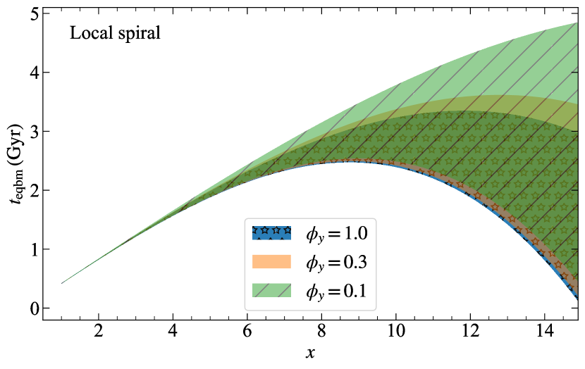
Figure 1: Metallicity equilibration time, $t_{\rm{eqbm}}$ plotted as a function of the dimensionless radius $x$ for three different values of the yield reduction factor, $\phi_{y}$, for a fiducial local spiral galaxy (see equation 19). Here, $x=r/r_{0}$, where $r_{0}=1\,\rm{kpc}$. The shaded bands correspond to solutions that cover all allowed values of the constant of integration $c_{1}$ in the solution to the metallicity equation (see Section 2.3). Since, $t_{\rm{eqbm}}$ is substantially smaller than the Hubble time $t_{\rm{H(0)}}$ and comparable to the molecular gas depletion time $t_{\rm{dep,H_{2}}}$, metallicity gradients in local spirals are in equilibrium.

3.1 Local spirals

For local spirals, we select the outer boundary of the star-forming disc to be $15\,\rm{kpc}$, thus $x_{\rm{max}}=15$, reminding the reader that $x=r/r_{0}$ where $r_{0}=1\,\rm{kpc}$. We first study the metallicity equilibration time ($t_{\rm{eqbm}}$) to see if metallicity gradients in these galaxies have attained equilibrium, so that the model can be applied to them. Figure 1 shows the value of $t_{\rm{eqbm}}$ we find from equation 19 as a function of $x$ for local spirals for different values of the yield reduction factor, $\phi_{y}$; the bands shown correspond to solutions covering all allowed values of the integration constant $c_{1}$. It is clear from Figure 1 that $t_{\rm{eqbm}}<t_{\rm{H(0)}}$ for all possible $\phi_{y}$ and $c_{1}$, so we conclude that the gradients in local spirals are in equilibrium. Additionally, $t_{\mathrm{eqbm}}\sim t_{\mathrm{dep,H_{2}}}$ for local spirals ($1-3\,\rm{Gyr}$, e.g., Wong & Blitz 2002; Bigiel et al. 2008; Saintonge et al. 2012; Leroy et al. 2013; Huang & Kauffmann 2014), implying that the metallicity distribution reaches equilibrium on timescales comparable to the molecular gas depletion timescale. The model also predicts that central regions of local spirals should achieve equilibrium earlier than the outskirts, however, this is somewhat sensitive to the choice of $c_{1}$ and $\phi_{y}$ as we can see from Figure 1 (see also, Figure 4 of Belfiore et al. 2019). Our equilibrium timescales are also consistent with our naive expectation as stated above: long compared to the timescale for local fluctuations to damp, but shorter than the time required for the total metallicity to reach equilibrium.

Figure 2 presents the family of radial metallicity distributions we obtain from the model for local spirals; the different lines correspond to varying choices of the outer boundary condition $c_{1}$, from the minimum to the maximum allowed. We report in the text annotations that accompany these curves the range of gas- and SFR-weighted mean metallicities $\overline{\mathcal{Z}}_{\Sigma_{g}}$ and $\overline{\mathcal{Z}}_{\dot{\Sigma}_{\star}}$, and metallicity gradients $\nabla(\log_{10}\mathcal{Z})$, spanned by the models shown. To aid in the interpretation of these results, in Figure 3 we also show the magnitudes of the various terms in the numerator on the right hand side of equation 19, which represent, respectively, the relative importance of advection, diffusion, metal production (reduced by metal ejection in outflows), and cosmological accretion in determining the metallicity gradient. We use this figure to read off which processes are dominant in different parts of the disc. While the source and the accretion terms fall off in the outermost regions due to the $1/x^{2}$ dependence, the advection and diffusion terms slightly increase with $x$, thereby resulting in a shorter metal equilibration time in the outermost regions as compared to intermediate regions, as we see in Figure 1. Thus, transport processes in the outer regions play an important role in establishing metal equilibrium in local spirals.

There are several noteworthy features in these plots. First, note how the solution asymptotically reaches a particular value of the central metallicity. We choose to set $\mathcal{Z}_{r_{0}}$ to this value, but we emphasise that the behaviour of the solution does not depend on this choice except very close to $x=1$: if we choose a different value of $\mathcal{Z}_{r_{0}}$, the solution is (by construction) forced to this value close to $x=1$, but returns to the asymptotic limit for $x\gtrsim 1.1$. Indeed, we shall see that this is a generic feature for all of our cases: the limiting central metallicity is set by a balance between two dominant processes, and can be deduced analytically by equating the two dominant terms in equation 41. For the case of local spirals, the two dominant terms throughout the disc are production and accretion, as we can read off from Figure 3. The balance between these two processes gives

$$\mathcal{Z}_{r_{0}}=\frac{\mathcal{S}}{\mathcal{A}}\,\,\,\,\left[\mathrm{Local}\,\mathrm{spirals}\right]\,.$$ (48)

This matches the conclusions of Finlator & Davé (2008) regarding the total metallicity. However, we show below in Section 3.2 that this conclusion holds only for local, massive galaxies, since other processes like metal transport also play a significant role in low mass galaxies as well as at high redshift. Using the above definition of $\mathcal{Z}_{r_{0}}$, we can now express $c_{1}$ in a more physically-meaningful way

$$c_{1}=\frac{1}{\sqrt{\mathcal{P}^{2}+4\mathcal{A}}}\left.\frac{\partial\mathcal{Z}}{\partial x}\right|_{r=r_{0}}\,.$$ (49)

Thus, for local spirals, $c_{1}$ essentially describes the metallicity gradient at $r_{0}$.

Second, both the central metallicity $\mathcal{Z}_{r_{0}}$ and the mean metallicity $\overline{\mathcal{Z}}$ decrease with decreasing $\phi_{y}$, as expected; we obtain mean metallicities close to Solar, as expected for massive local spirals, for $\phi_{y}$ fairly close to unity. Thus our models give reasonable total metallicities for local spirals if we assume that there is relatively little preferential ejection of metals, consistent with the results of recent simulations (Du et al., 2017; Tanner, 2020; Taylor et al., 2020). Note that some semi-analytic models find a high metal ejection fraction for spirals, but self-consistently following the evolution of the CGM subsequently leads to high re-accretion of the ejected metals (Yates et al., 2020). In the language of our model, this essentially implies a high $\phi_{y}$ when averaging over the metal recycling timescale for local spirals, consistent with our expectations.

Third, and most importantly for our focus in this paper, the value of $\phi_{y}$ has little effect on the metallicity gradient, as is clear from the similar range of gradients produced by the model for different $\phi_{y}$. Our models robustly predict a gradient $\nabla(\log_{10}\mathcal{Z})\approx-0.07$ to $0$ dex kpc^-1, in very good agreement with the range observed in local spirals (e.g., Zaritsky et al., 1994; Sánchez et al., 2014; Ho et al., 2015; Sánchez-Menguiano et al., 2016; Belfiore et al., 2017; Erroz-Ferrer et al., 2019; Mingozzi et al., 2020), and within the range provided by existing simpler models of metallicity gradients (Chiappini et al., 2001; Fu et al., 2009).

Apart from the mean gradient, we can also study the detailed shape of the metal distribution with the model. For the given input parameters as in Table 2, the model features a nearly-flat metal distribution in the inner galaxy for all allowed values of $c_{1}$. Such flat gradients in the inner regions are commonly observed in local spirals (Moran et al., 2012; Belfiore et al., 2017; Mingozzi et al., 2020), and have been attributed to metallicity reaching saturation in these regions (Zinchenko et al., 2016; Maiolino & Mannucci, 2019), although the flatness depends on the metallicity calibration used (Yates et al., 2020, Figure 4). This is also the case for our models of spirals, since the flat region corresponds to the part of the disc where the metallicity is set by the balance between metal injection and dilution by metal-poor infall (c.f. Figure 3). For comparison, we also show in Figure 2 the measured average metallicity profiles in local spirals observed in the MaNGA survey (Belfiore et al., 2017) using two different metallicity calibrations (Pettini & Pagel, 2004; Maiolino et al., 2008), where we have adjusted the overall metallicity normalisation by 0.02 dex so that the model profiles overlap with the data. We see that the profiles produced by the model are in reasonable agreement with that seen in the observations (see also, Sánchez-Menguiano et al. 2018).

Several works have also noted that local spirals with higher gas fractions (at fixed mass) show steeper metallicity gradients (Carton et al., 2015; De Vis et al., 2019; Pace et al., 2020). In the language of the Krumholz et al. (2018) model, a higher gas fraction implies a higher value of $f_{g,Q}$ and $f_{g,P}$. Increasing these parameters leads to an increase in the source term $\mathcal{S}$, which gives rise to steeper metallicity gradients in the model, consistent with the above observations. Moreover, a higher gas fraction (i.e., higher $f_{g,Q}$ and $f_{g,P}$) also results in a rather steep metallicity profile in the inner disc, thus giving slightly lower metallicities in the inner disc as compared to the fiducial case above, consistent with the standard picture of galaxy chemical evolution (Tinsley 1972, 1973; see also, Pace et al. 2020).

It is difficult to provide robust predictions for the metal distribution in the outer parts of the galaxy without further constraining $c_{1}$. The outer-galaxy metal distribution in the model is also sensitive to parameters like the galaxy size and the CGM metallicity. The result of these uncertainties is that depending on the choice of $c_{1}$, the model can produce both nearly-flat and quite steep metal distributions in the outer parts of the galaxy. A steep drop in the metallicity in the outer disc has been observed in several local spirals (Moran et al., 2012), but is dependent on the metallicity calibration used (Carton et al., 2015). In our models, this region corresponds to where cosmological accretion of metal-poor gas onto the disc becomes less important than inward advection of metal-poor gas through the disc – a process whose rate we would expect to be correlated with the available mass supply in the far outer disc, as measured by H i. Note that the gradient can also flatten again in the outermost regions in the disc (Werk et al., 2011; Sánchez et al., 2014; Sánchez-Menguiano et al., 2016; Bresolin, 2019); however, these regions typically have insufficient spatial resolution (Acharyya et al., 2020a) as well as significant diffused ionised gas emission, both of which can cause the gradients to appear flatter than their true values (Kewley et al., 2019a, Section 6). Given the uncertainties in the model as well as observations of metallicities in the outer discs in spirals, it is not yet obvious if the metal distribution in the outer disc in the model can be validated against the available observations. Thus, we do not study these regions with our model. This analysis also shows that linear fits to the metallicity profiles is a crude approximation to the true underlying metallicity distribution in local spiral galaxies.

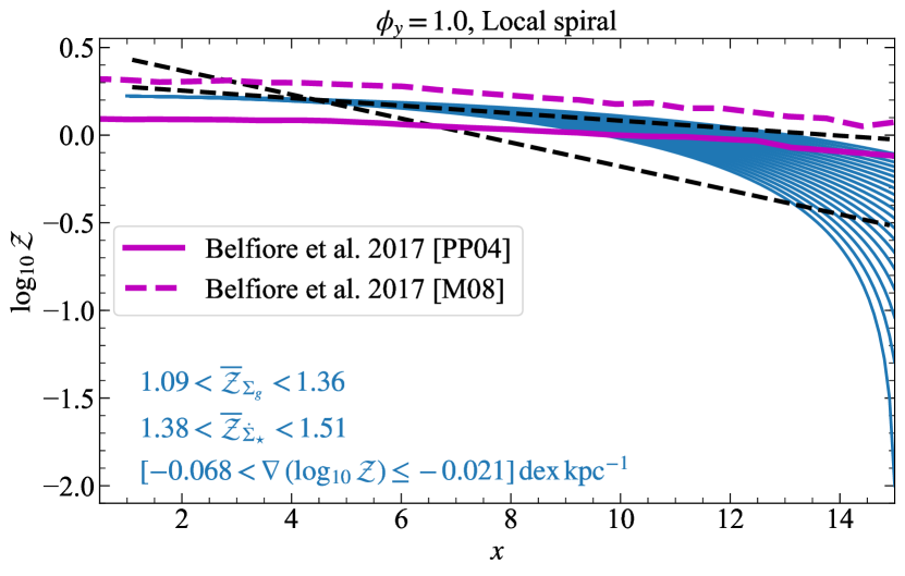
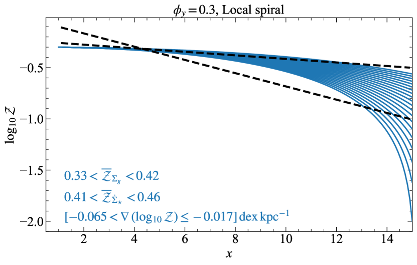
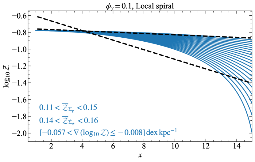
Figure 2: Metallicity ($\mathcal{Z}=Z/Z_{\odot}$; blue lines) as a function of dimensionless radius ($x=r/r_{0}$ with $r_{0}=1\,\rm{kpc}$) produced by the model for a fiducial local spiral galaxy with input parameters listed in Table 1 and Table 2, for different values of the yield reduction factor, $\phi_{y}$. The analytic solution to the metallicity evolution equation is given by equation 41. The slope of the linear fit to the model gradients between $x=1-15$ (black, dashed lines) gives the metallicity gradient that can be compared against simulations and observations. The blue coloured curves show the acceptable parameter space of the gradients based on the constraints on the constant of integration, $c_{1}$, using the boundary conditions criteria described in Section 2.3. The metallicity at the inner edge of the disc (referred to as the central metallicity in the text), $\mathcal{Z}_{r_{0}}$, is set by the balance between source and accretion for local spirals (see equation 48). $\overline{\mathcal{Z}}_{\Sigma_{g}}$ and $\overline{\mathcal{Z}}_{\dot{\Sigma}_{\star}}$ represent the range of mass-weighted and SFR-weighted mean equilibrium metallicities produced by the solution, respectively (see equation 46). We expect $\phi_{y}$ closer to unity for local spirals, implying that metals in these galaxies are well-mixed with the ISM before they are ejected. Finally, in the top panel we overplot the average metallicity profiles observed in local spirals in the MaNGA survey by Belfiore et al. (2017) using the PP04 (Pettini & Pagel, 2004) and M08 (Maiolino et al., 2008) calibrations, adjusting the normalisation to overlap with the model profiles.

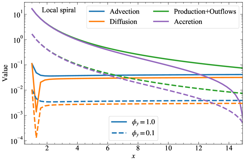
Figure 3: Absolute values of different terms in the numerator of equation 19 that collectively build the metallicity gradient in local spirals, for a fixed $\mathcal{Z}_{\rm{CGM}}=0.1$ and fixed $c_{1}$ for different yield reduction factors, $\phi_{y}$. These terms are defined in equation 14. The leading terms that set the gradients in local spirals are metal production and accretion of gas onto the galaxy, whereas advection and diffusion play a subdominant role in local spirals, due to the small velocity dispersion, $\sigma_{g}$. Note that the sharp feature in the diffusion term near $x=1.3$ corresponds to the location where this term passes through zero as it changes sign; the term in fact behaves smoothly everywhere, but this behaviour appears as a sharp feature when plotted on a logarithmic axis.

3.2 Local dwarfs

Our model can also be applied to local dwarf galaxies that can be classified as rotation-dominated, e.g., the Large Magellanic Cloud (LMC), for which $v_{\phi}\sim 60\,\mathrm{km\,s^{-1}}$ and $\sigma_{g}\sim 7\,\mathrm{km\,s^{-1}}$ (Alves & Nelson, 2000). Such galaxies typically lie at the massive end of dwarfs ($M_{\star,\rm{LMC}}=2\times 10^{9}\,\rm{M_{\odot}}$, as reported in van der Marel 2006; Skibba et al. 2012), and possess an equilibrium gas disc to which the unified galaxy evolution model of Krumholz et al. (2018) can be applied. We set the outer disc radius to $6\,\mathrm{kpc}$ to find the gradient in the fiducial model, in line with the estimated gas disc size of local dwarfs ($r_{\rm{LMC}}\sim 4.3\,\rm{kpc}$, Westerlund 1990).

Figure 4 shows the metal equilibration time, $t_{\rm{eqbm}}$, for local dwarfs based on the parameters we list in Table 1 and Table 2. It is clear that metallicity gradients are in equilibrium in dwarfs, since $t_{\rm{eqbm}}<t_{\rm{H(0)}}$ as in the case of local spirals (see, however, Section 5.2.1 where we show that this may not be the case under certain circumstances). Contrary to local spirals, local dwarfs show a wide range of $t_{\mathrm{dep,H_{2}}}$, from a few hundred Myr to several Gyr (e.g., Bolatto et al. 2011; Bothwell et al. 2014; Hunt et al. 2015; Jameson et al. 2016; Schruba et al. 2017), similar to the scatter we find in $t_{\rm{eqbm}}$ (see also, Section 5.2.1).

Having established metal equilibrium in local dwarfs, we can now study the gradients produced by the model. Figure 5 shows the resulting metallicity versus radius for different $\phi_{y}$ (analogous to Figure 2), and Figure 6 shows the relative importance of the various processes (analogous to Figure 3).

In the case of local dwarfs, we see that $\mathcal{Z}_{r_{0}}$ is set by the balance between advection and diffusion, giving

$$\mathcal{Z}_{r_{0}}=\frac{\mathcal{S}}{\mathcal{A}}+c_{1}\left(1+\frac{\sqrt{\mathcal{P}^{2}+4\mathcal{A}}-\mathcal{P}^{2}-\mathcal{A}}{\sqrt{\mathcal{P}^{2}+4\mathcal{A}}+\mathcal{P}^{2}+\mathcal{A}}\right)\,\,\,\,\left[\mathrm{Local}\,\mathrm{dwarfs}\right]\,.$$ (50)

Using the above definition of $\mathcal{Z}_{r_{0}}$, we can express $c_{1}$ as

$$c_{1}=\frac{\sqrt{\mathcal{P}^{2}+4\mathcal{A}}+\mathcal{P}^{2}+\mathcal{A}}{\left[\mathcal{A}+\left(\mathcal{P}-1\right)\mathcal{P}\right]\sqrt{\mathcal{P}^{2}+4\mathcal{A}}}\left.\frac{\partial\mathcal{Z}}{\partial x}\right|_{r=r_{0}}\,.$$ (51)

Central metallicities are in the range $\mathcal{Z}_{r_{0}}\approx 0.2-0.6$ depending on the choice of $\phi_{y}$, in good agreement with that observed in local dwarfs, e.g., in the SMC and the LMC (Russell & Dopita, 1992; Westerlund, 1997), and M82 (Origlia et al., 2004). While $\mathcal{Z}_{r_{0}}$ depends only on $\mathcal{S}/\mathcal{A}$ in local spirals, it also depends on the choice of $c_{1}$ for local dwarfs, implying that it is independent of the disc properties in the former case but not in the latter. Similarly, mean metallicities range from $\overline{\mathcal{Z}}\sim 0.1-0.5$ as $\phi_{y}$ varies from $\approx 0.1-1$; both observations (Martin et al., 2002; Strickland & Heckman, 2009; Chisholm et al., 2018) and numerical simulations (Emerick et al., 2018; Emerick et al., 2019) suggest that dwarfs suffer considerable direct metal loss, so $\phi_{y}$ considerably smaller than unity seems likely.

As opposed to spirals, our models predict that gradients are not necessarily flat in the inner regions of dwarfs, which is also consistent with observations (Belfiore et al., 2017; Mingozzi et al., 2020). The reason for this difference is due to different physical processes dominating in the two types of galaxies: accretion versus metal production in spirals, and advection versus production in dwarfs. Consequently, we predict linear gradients for local dwarfs that are steeper than the ones for local spirals at fixed $\phi_{y}$ and $c_{1}$. For the smaller values of $\phi_{y}$ expected in local dwarfs, we expect gradients in the range $\sim-0.01$ to $-0.15\,\rm{dex\,kpc^{-1}}$, implying a larger scatter in the gradients measured in local dwarfs as compared to that in local spirals, consistent with observations (Mingozzi et al., 2020, Figure 12). The metallicity profiles produced by the model for smaller values of $\phi_{y}$ are also in agreement with that observed in the MaNGA survey (Belfiore et al., 2017), as we show in Figure 5, where we have adjusted the overall metallicity normalization by 0.15 dex to facilitate a comparison of the data and the model profiles. Further, the larger range of gradients in low mass local galaxies as compared to massive galaxies allowed within the framework of our model is also relevant and necessary for reproducing the observed steepening of gradients with decreasing galaxy mass (Bresolin, 2019, Figure 10).

Although this is not illustrated in Figure 5, we also find that the magnitude of the gradient is quite sensitive to both the “floor” velocity dispersion supplied by star formation, $\sigma_{\rm{sf}}$, and the Toomre $Q$ parameter, since these two jointly set the strength of advection and in this case, $\sigma_{\rm{sf}}\sim\sigma_{g}$. Thus, we expect that gradients for local dwarfs will show more scatter than those for local spirals. It is interesting to note that there is a similarly large scatter in simulations of dwarf galaxies, with some groups (e.g., Tissera et al., 2016) finding steeper gradients for dwarfs as compared to spirals whereas others (e.g. Ma et al., 2017) finding the opposite. This difference between the simulations has been attributed to the strength of feedback, which, in the language of our model, corresponds to variations in $\sigma_{\rm sf}$ and $\phi_{y}$; thus the sensitivity of our model is at least qualitatively consistent with the strong dependence of feedback strength observed in simulations.

Figure 4: Same as Figure 1, but for local dwarfs. Here, $t_{\rm{eqbm}}<t_{\rm{H(0)}}$, implying that the metallicity gradients in local dwarfs are also in equilibrium, even in the case of low $\phi_{y}$ (see the text for a discussion on $t_{\rm{dep,H_{2}}}$ for local dwarfs). The corresponding metallicity gradients are plotted in Figure 5.

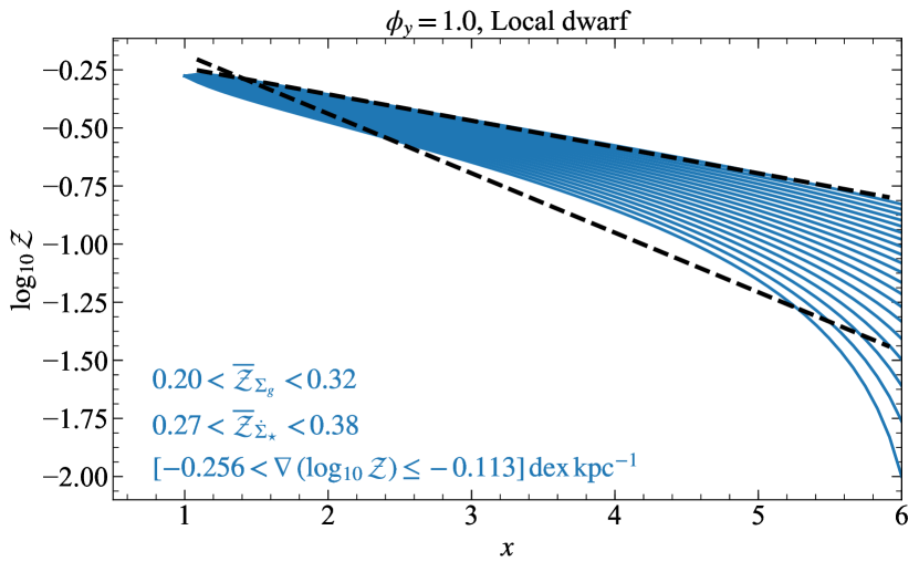
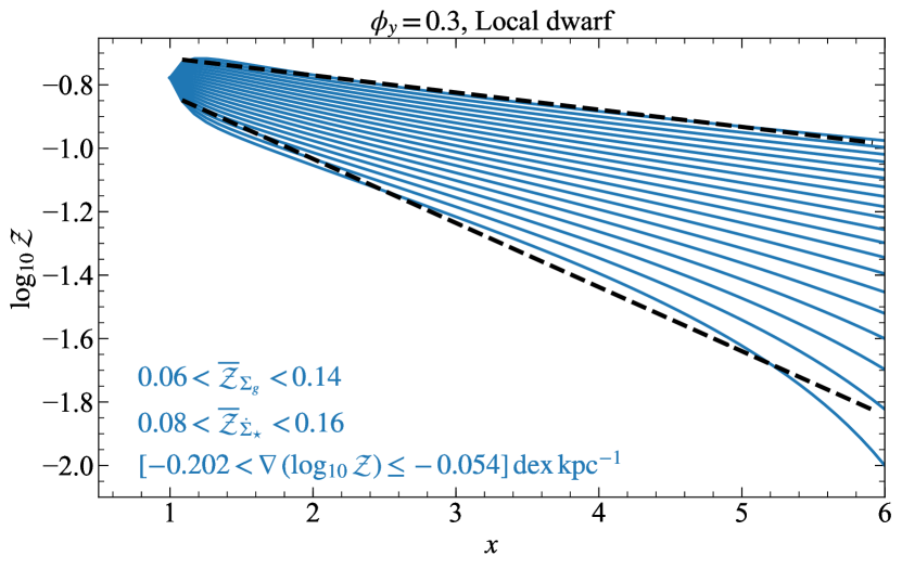
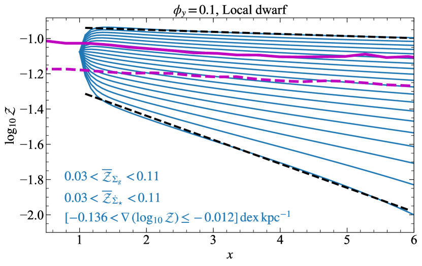
Figure 5: Same as Figure 2, but for local dwarfs. Here, $\mathcal{Z}_{r_{0}}$ is set by the balance between advection and diffusion, whereas metallicities in the disc are set by the balance between advection and source. The sharp rise and fall in the profile at $x=1$ is an artefact of the choice of the constant of integration $c_{1}$ used to calculate $\mathcal{Z}_{r_{0}}$ (see equation 51). The gradients are particularly sensitive to the strength of advection for local dwarfs since turbulence due to star formation feedback is comparable to that due to gravity, $\sigma_{\rm{sf}}\sim\sigma_{g}$. When they are exactly equal, advection vanishes, and the gradients may not be in equilibrium (see Section 5.2.1). In the last panel we also plot (purple lines) the average metallicity profiles observed in local dwarfs in the MaNGA survey; see Figure 2.

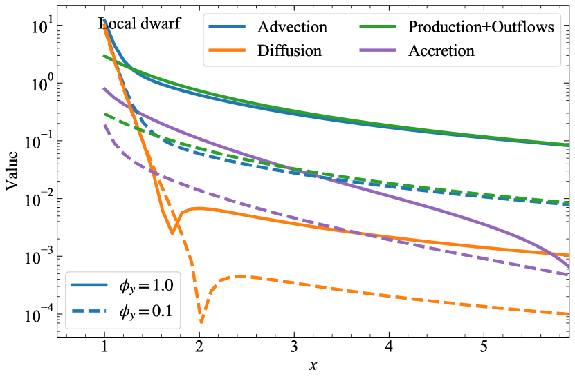
Figure 6: Same as Figure 3, but for local dwarfs. The dominant terms that set the gradients in local dwarfs are advection and diffusion (in the inner disc) and source and advection (in the outer disc).

3.3 High-redshift galaxies

Massive galaxies at high-$z$ are primarily rotation-dominated with underlying disc-like structures (Weiner et al., 2006; Förster Schreiber et al., 2009, 2018; Wisnioski et al., 2011, 2015, 2019; Wuyts et al., 2011; Di Teodoro et al., 2016; Simons et al., 2017; Übler et al., 2019). Thus, we can apply the model to these galaxies. For high-$z$ galaxies, we set the outer disc radius to $10\,\mathrm{kpc}$ to find the gradient in the fiducial model, acknowledging that galaxies at higher redshifts are smaller than that in the local Universe (e.g., Queyrel et al., 2012; van der Wel et al., 2014). Hereafter, we work with $z=2$ as a fiducial redshift. Figure 7 shows the metal equilibration time for high-$z$ galaxies. It is clear that $t_{\rm{eqbm}}<t_{\rm{H(z)}}$, so that the equilibrium solution can be applied to these galaxies. Following Tacconi et al. (2018, 2020), if we assume that a main sequence high-$z$ galaxy follows $t_{\rm{dep,H_{2}}}\propto(1+z)^{-0.6}$, it implies that $t_{\rm{dep,H_{2}}}\sim 0.5-1.5\,\rm{Gyr}$ for high-$z$ galaxies, which is comparable with $t_{\rm{eqbm}}$ as above.

Figure 8 shows the equilibrium metallicity distributions we obtain for a fiducial high-$z$ galaxy with parameters listed in Table 1 and Table 2, and Figure 9 shows our usual diagnostic diagram comparing the importance of different processes. Examining this diagram near $x=1$, it is clear that, as is the case for local dwarfs, the central metallicity $\mathcal{Z}_{r_{0}}$ is set by the balance between advection and diffusion, which gives

$$\mathcal{Z}_{r_{0}}=\frac{\mathcal{S}}{\mathcal{A}}+c_{1}\left(1+\frac{\sqrt{\mathcal{P}^{2}+4\mathcal{A}}-\mathcal{P}^{2}-\mathcal{A}}{\sqrt{\mathcal{P}^{2}+4\mathcal{A}}+\mathcal{P}^{2}+\mathcal{A}}\right)\,\,\,\,\left[\mathrm{High}-z\right]\,.$$ (52)

It varies between $\mathcal{Z}_{r_{0}}=0.3$–$0.7$ depending on the value of $\phi_{y}$, in good agreement with observed metallicities in high-$z$ galaxies in the mass range we consider (Erb et al., 2006; Yabe et al., 2012), with $c_{1}$ same as that in equation 51. While the absolute metallicity depends on $\phi_{y}$, the metallicity gradients for the most part do not – we find $\nabla(\log_{10}\mathcal{Z})\approx-0.15$ to $-0.05$ dex kpc^-1, with order-of-magnitude variations in $\phi_{y}$ only altering these values by a few hundredths.

The gradients we find for high-$z$ galaxies are steeper than for local spirals, and the distributions are steeper at small radii than at larger radii, the opposite of our finding for local spirals. Figure 9 shows why this is the case: gradients over most of the radial extent of high-$z$ galaxies are set by the balance between source and advection, whereas accretion, which dilutes the gradients in local spirals, is sub-dominant. The fundamental reason for this change is due to the vastly higher velocity dispersions of high-$z$ galaxies, which increase the importance of the advection term ($\mathcal{P}\propto(1-\sigma_{\mathrm{sf}}/\sigma_{g})$) while suppressing the accretion term ($\mathcal{A}\propto\sigma^{-3}_{g}$); this effect is partly diluted by the higher accretion rates found at high-$z$ (equation 34), but the net change at high redshift is nonetheless toward a smaller role for accretion onto discs and a larger role for transport through them. We discuss this further in detail in Section 4.

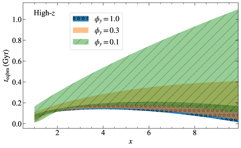
Figure 7: Same as Figure 1, but for high-$z$ galaxies. The corresponding equilibrium metallicity gradients are plotted in Figure 8.

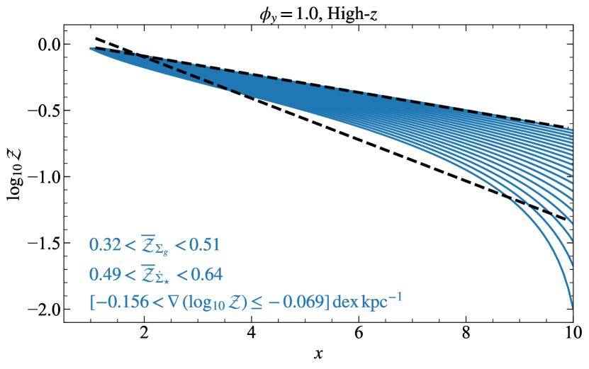
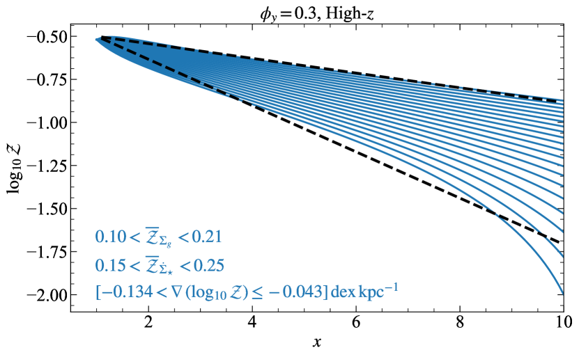
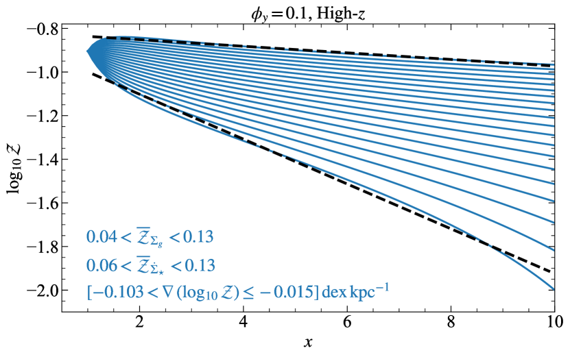
Figure 8: Same as Figure 2, but for high-$z$ galaxies. Here, $\mathcal{Z}_{r_{0}}$ is set by the balance between diffusion and advection.

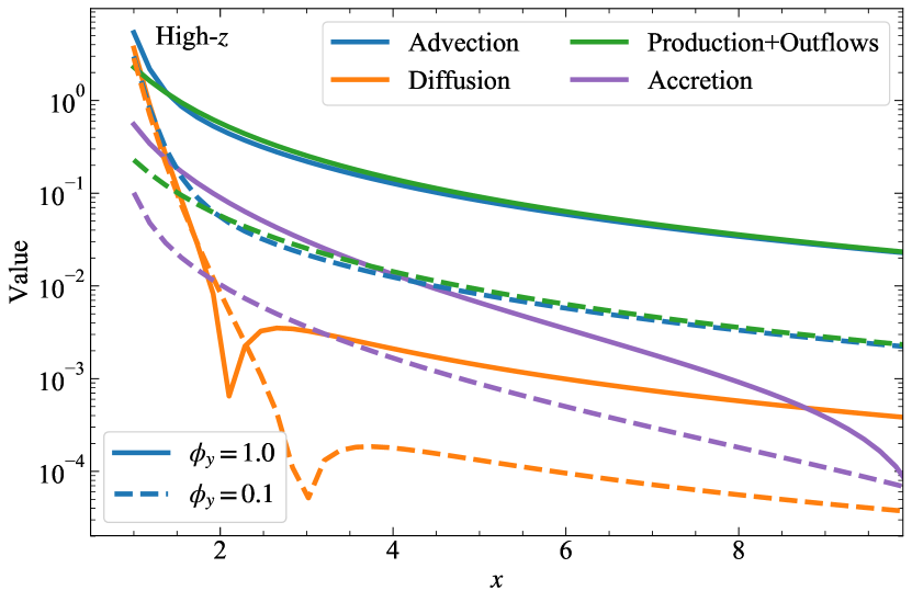
Figure 9: Same as Figure 3, but for high-$z$ galaxies. Here, the metallicities in the disc are set by the balance between source and advection, due to efficient radial transport of the gas.

4 Cosmic evolution of metallicity gradients

A significant advantage of our model compared to previous analytic efforts, is that it makes meaningful predictions for how galaxy metallicity gradients have evolved across cosmic time. This is the case because we do not have the freedom to adjust parameters such as radial inflow rates and profiles of star formation rate to match any given observed galaxy. Instead, these parameters are either prescribed directly from our galaxy evolution model or depend on parameters that are directly observable (e.g., galaxy velocity dispersions). The basic inputs to our model are the halo mass $M_{\rm{h}}$ and the gas velocity dispersion $\sigma_{g}$ as a function of $z$. We consider three different ways of selecting galaxies that yield different tracks of $M_{h}(z)$ (see below for details), while we take the evolution of $\sigma_{g}(z)$ from the observed correlation obtained by Wisnioski et al. (2015, see their equation 8)

$$\sigma_{g}(z)=\frac{v_{\phi}(z)f_{\mathrm{gas}}(z)}{\sqrt{2\left(\beta+1\right)}},$$ (53)

where $f_{\rm{gas}}$ is the molecular gas fraction of the galaxy (Genzel et al., 2011; Genel et al., 2012; Tacconi et al., 2013; Genzel et al., 2015; Faucher-Giguère, 2018). This scaling is subject to considerable observational uncertainty, the implications of which we explore in Appendix B. We follow Wisnioski et al. (2015) to find $f_{\rm{gas}}$ as a function of $M_{\star}$ and $z$ from Tacconi et al. (2013) and Whitaker et al. (2014), as it is now known that $f_{\rm{gas}}$ decreases with cosmic time and stellar mass (Leroy et al., 2008; Saintonge et al., 2011; Geach et al., 2011; Davé et al., 2012; Tacconi et al., 2013, 2018; Morokuma-Matsui & Baba, 2015; Isbell et al., 2018). We note that Wisnioski et al.’s sample is limited to massive galaxies ($M_{\star}>10^{10}\,\rm{M_{\odot}}$), and there are no observations available for lower-mass galaxies. For this reason we instead follow the results of the IllustrisTNG simulations to obtain $\sigma_{g}(z)$ (Pillepich et al., 2019, see their Figure 12a) for stellar masses below $10^{10}\,\rm{M_{\odot}}$. Finally, note that all the gradients we produce from the model in this section are in equilibrium across the redshifts we use, since $t_{\rm{eqbm}}<t_{\rm{H(z)}}$.

4.1 Trends for a Milky Way-like galaxy across redshift

We first study how the gradient in a Milky Way-like galaxy has evolved over time using our model. We only need one parameter to begin with: $v_{\phi}$ at $z=0$. We set this to $220\,\rm{km\,s^{-1}}$ (Bland-Hawthorn & Gerhard, 2016). Then, we use equation 35 to calculate $M_{\mathrm{h}}\,(z=0)$ for a fixed $c=15$. Using $M_{\mathrm{h}}\,(z=0)$ as boundary condition, we integrate equation 34 to find $M_{\mathrm{h}}\,(z)$, keeping in mind that this equation represents an average evolution of $M_{\mathrm{h}}\,(z)$ that may not necessarily apply to the Milky Way. Then, we utilize $M_{\mathrm{h}}\,(z)$ to find $v_{\phi}\,(z)$, by changing the concentration parameter ($c$) as an empirical third-order polynomial fit, following Zhao et al. (2009). This ensures that as we change $z$, we self-consistently find $M_{\rm{h}}$ and $v_{\phi}$. We adopt a simple linear variation for the outer edge of the star-forming disc, $x_{\rm{max}}$, as a function of $z$ such that it is 15 at $z=0$ and 10 at $z=2$. Similarly, we vary $f_{\rm{sf}}$ between 0.5 and 1 across redshift, keeping in mind that $f_{\rm{sf}}$ cannot be more than 1 at any redshift. For simplicity, we fix the other parameters as follows: $\beta=0$, $f_{g,Q}=f_{g,P}=0.5$, $\sigma_{\mathrm{sf}}=7\,\mathrm{km\,s^{-1}},\,Q_{\mathrm{min}}=1.5$ and $\mathcal{Z}_{\rm{CGM}}=0.1$.

We show the resulting evolution of the gradient in Figure 10. The model predicts a steepening of the gradient in Milky Way-like galaxies over time, with the exception of a very recent flattening, between $z\approx 0.15$ and 0. We can understand these trends in terms of the dimensionless parameters $\mathcal{S}$, $\mathcal{P}$, and $\mathcal{A}$ that describe the relative importance of in situ metal production, radial advection, and cosmological accretion with diffusion, respectively. The source term $\mathcal{S}$ will always make the gradients steeper because of the steep radial profile of $\dot{\Sigma}_{\star}$, and it is either $\mathcal{P}$ or $\mathcal{A}$ that balances $\mathcal{S}$ to give rise to flatter gradients. The steepest gradients at $z\approx 0.15$ correspond to when both $\mathcal{P}$ and $\mathcal{A}$ are at their weakest compared to $\mathcal{S}$. We can understand the trends on either side of this maximum in turn.

First, let us focus on the recent epoch, $z\lesssim 0.15$. During this period, cosmological accretion ($\mathcal{A}$) is more important than radial transport ($\mathcal{P}$), and accretion and metal production depend on the galaxy rotational velocity as $\mathcal{A}\propto v_{\phi}^{3.3}$ and $\mathcal{S}\propto v_{\phi}^{2}$, respectively. Thus, as the galaxy grows in mass, dilution by accretion gets stronger compared to metal production, leading to the recent flattening in the model. However, this can change if the metal production is underestimated, e.g., due to ignoring the contribution from long-term wind recycling (Leitner & Kravtsov, 2011).

During this epoch advection is more important than accretion, $\mathcal{P}>\mathcal{A}$. The ratio of the two effects, $\mathcal{P}/\mathcal{A}$, is large at high redshift, and decreases systematically towards the present day, ultimately reaching $\mathcal{P}/\mathcal{A}\approx 1$ at $z\approx 0.15$. This transition is ultimately driven by the systematic decrease in galaxy velocity dispersions with redshift, as already discussed in the context of our high-$z$ galaxy models (Section 3.3): higher velocity dispersions are strongly correlated with higher rates of radial inflow through a galaxy, so that for a Milky Way progenitor at $z\gtrsim 1$, radial inflow transports metal-poor gas into galaxy centres $\sim 10\times$ faster than cosmological accretion ($\mathcal{P}/\mathcal{A}\approx 10$) – despite the fact that the absolute accretion rate is higher at $z\gtrsim 1$ than it is today. Similarly, the ratio of radial inflow to metal production, $\mathcal{P}/\mathcal{S}$, scales with velocity dispersion as $\sigma_{g}^{2}$ (for $\sigma_{g}\gg\sigma_{\rm sf}$), so radial inflow also becomes more important relative to metal production as we go to higher redshift and higher velocity dispersion. This explains the flatness of gradients at high redshift. This transition from radial advection being dominant to being unimportant is mirrored in the transition from gravity-driven to star formation feedback-driven turbulence from high- to low-$z$ (Krumholz et al., 2018), as we noted earlier in Section 3.3.

Lastly, we find that diffusion is sub-dominant compared to both advection and accretion at all cosmological epochs, because $\mathcal{P}$ and $\mathcal{A}$ are never both less than unity at the same time. Thus, while diffusion can have some effects on the metallicity distributions, particularly towards galaxy centres (cf. Figure 6), as well as on metal equilibrium timescales (cf. Figure 1), it is generally unimportant for setting galaxy metallicity gradients.

4.1.1 Comparison with observations

There is extensive data on the history of the Galaxy’s metallicity gradient, as summarised by Mollá et al. (2019, see their Table 1), and on the history of the gradients in a number of other nearby galaxies. The general outcome of these studies is that gradients measured in H ii regions (which trace the current-day metal distribution) are steeper than those measured in planetary nebulae or open clusters (which trace older populations) (Stanghellini & Haywood, 2010; Stanghellini et al., 2010, 2014; Sanders et al., 2012; Stasińska et al., 2013; Magrini et al., 2016). This implies a steepening of the gradient with time in Milky Way-like galaxies, however, this should be treated with caution because measured metallicity gradients in the Galaxy are subject to large errors arising from uncertainties in estimating the ages of the planetary nebulae (Maciel et al., 2010; Cavichia et al., 2011), and due to radial migration that could result in a movement of the planetary nebulae away from their origin (Minchev et al., 2013).

To allow a quantitative comparison of these observations with our model, we show measurements of the metallicity gradient for the Milky Way as a function of lookback time from Stanghellini et al. (2010) as yellow circles in Figure 10. The data for the Milky Way (as well as other local spirals, see Stanghellini et al. 2014) are in qualitative agreement with the predictions from our model. However, we also note that for our model to agree quantitatively with the measurements, we would need $\phi_{y}$ to be lower at high redshift, and increase towards unity today. Such a change in $\phi_{y}$ is plausible and is consistent with our expectation that $\phi_{y}$ should be close to unity in more massive galaxies like the present-day Milky Way, and smaller than unity in less massive galaxies with shallower potential wells, such as the Milky Way’s high-$z$ progenitors. However, the exact form of this evolution is not independently predicted by our model.

4.1.2 Comparison with simulations

On Figure 10, we also overplot results from Feedback In Realistic Environments (FIRE) simulations (Hopkins et al., 2014, 2018) of a Milky Way-like galaxy (m12i) discussed in Ma et al. (2017). This simulation finds that metallicity gradients are unstable until $z\sim 1$, after which they steepen and stabilise to an equilibrium value. This transition is primarily due to the formation of a robust galactic disc that cannot be disrupted again due to internal or external feedback. While the quantitative trends slightly differ at some redshifts between our model and the simulation, which is not unexpected given that the exact implementation of the feedback and measurements of the gradients are different, there is a very good qualitative match. This match also implies that Milky Way-like galaxies would have had lower $\phi_{y}$ in the past as compared to the present day, as outflows were more common and stronger in the past due to higher SFR and could have ejected a larger fraction of metals not mixed with the ISM (Muratov et al., 2015; Ma et al., 2017); such a scenario has received support from recent high-resolution simulations that spatially resolve multi-phase galactic outflows, and find that the metal enrichment factor in both the cold ($<2\times 10^{4}\,\rm{K}$) and hot ($>5\times 10^{5}\,\rm{K}$) outflows increases with the SFR surface density (Kim et al., 2020). We can also compare our results with those of Gibson et al. (2013), where the authors study two identical simulation suites with either weak or enhanced stellar feedback, called MUGS and MaGICC, respectively (Stinson et al., 2010). The authors find that gas phase metallicity gradients are steep at high redshift in MUGS, whereas they are flat in MaGICC, clearly revealing the close correlation between feedback and metallicity gradients in galaxies. One of their simulated galaxies, MaGICC g1536, resembles the Milky Way in terms of its stellar mass, so we also compare our model results to that simulation in Figure 10. Again, we find qualitative similarities between the simulations and the model.

Figure 10: Metallicity gradient versus redshift (and lookback time) for a Milky Way-like galaxy. Different symbols show different yield reduction factors, $\phi_{y}$, while symbol colour shows the ratio of the dimensionless numbers $\mathcal{P}/\mathcal{A}$ that describe the relative importance of radial transport and cosmological accretion, respectively. The grey curve is taken from FIRE simulations of a Milky Way-like galaxy (Ma et al., 2017) whereas the dashed, black curve is from the MaGICC g1536 simulation by Gibson et al. (2013). The orange points are from observations of H ii regions, planetary nebulae and open clusters by Stanghellini & Haywood (2010), with horizontal errorbars representing the uncertainties in the ages of planetary nebulae and open clusters. The data, simulations and the model all qualitatively show that gradients in Milky Way-like galaxies have steepened over time, with the model predicting a mild flattening between $z=0.15$ and present-day. In the model, this evolution is driven by a transition from the advection-dominated regime ($\mathcal{P}/\mathcal{A}>1)$ to the accretion-dominated regime ($\mathcal{P}/\mathcal{A}<1)$ around $z\approx 0.15$. Such a transition in metallicity gradients is mirrored in the transition in gravity-driven turbulence at high $z$ to star formation feedback-driven turbulence at $z=0$ (Krumholz et al., 2018).

4.2 Trends for matched stellar mass galaxies across redshift

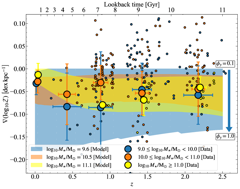
Figure 11: Trends in metallicity gradients as a function of redshift and lookback time. Colored markers represent individual galaxies within the three $M_{\star}$ bins as shown in the legend, with bigger markers representing binned averages of non-positive gradients across different redshift bins, and errorbars representing the scatter in the data within each redshift bin. The averages at $z=0$ are taken from local surveys (Sánchez et al., 2014; Sánchez-Menguiano et al., 2016; Belfiore et al., 2017; Mingozzi et al., 2020). The high-redshift compilation data is taken from Queyrel et al. (2012); Swinbank et al. (2012); Stott et al. (2014); Leethochawalit et al. (2016); Wuyts et al. (2016); Molina et al. (2017); Carton et al. (2018); Förster Schreiber et al. (2018); Wang et al. (2020); Curti et al. (2020), and is inhomogeneous, with systematic issues within the different measurements (see Section 4.2). The colored bands represent models at three $M_{\star}$ values, with the spread resulting from different yield reduction factors $\phi_{y}$, as marked by the arrow besides the shaded region. This spread in the model is largest for the low mass galaxies. While the general trend of mild evolution of gradients across redshift holds true, the models uncover the underlying variations due to galaxies transitioning from advection- to accretion-dominated regimes between $z=2.5$ and $0$, as is visible in the binned data averages. Some data points lie outside the range of the plot, and we do not include those for the purposes of studying the average trends of the data with the model.

In this section, we study the mass-averaged trends of metallicity gradients across cosmic time. For this purpose, we use a compilation of observations of metallicity gradients in (lensed and un-lensed) galaxies spanning $0\leq z\leq 2.5$ (Queyrel et al., 2012; Swinbank et al., 2012; Stott et al., 2014; Leethochawalit et al., 2016; Wuyts et al., 2016; Molina et al., 2017; Carton et al., 2018; Förster Schreiber et al., 2018; Wang et al., 2020; Curti et al., 2020), and we also include results from local surveys (Sánchez et al., 2014; Sánchez-Menguiano et al., 2016; Belfiore et al., 2017; Mingozzi et al., 2020; Acharyya et al., 2020b).

Before proceeding, we warn the reader that there are many uncertainties inherent in comparing metallicity gradients across samples and across cosmic time. For example, most studies in the compiled dataset rely on strong line calibrations that use photoionisation models or electron temperature-based empirical relations to measure metallicity gradients, and the variations between different calibrations can be as high as 0.1 dex per effective half-light radius (Moustakas et al., 2010; Poetrodjojo et al., 2019, 2021; Mingozzi et al., 2020). Further, since many high-$z$ metallicity gradient measurements rely on nitrogen whereas low-$z$ measurements use a larger set of (optical) emission lines, we also expect some systematic differences in these measurements with redshift (Carton et al., 2018; Kewley et al., 2019a). Using nitrogen can also lead to systematically flatter gradients due to different scalings of N/O with O/H in galaxy centres and outskirts (Schaefer et al., 2020). Lastly, it is not yet clear if strong line metallicity calibrations developed for the ISM properties of local galaxies are also applicable at high-$z$, where ISM electron densities, ionisation parameters, N/O ratios, or other conditions may differ from those in local galaxies (e.g., Shirazi et al., 2014; Sanders et al., 2016; Onodera et al., 2016; Kashino et al., 2017; Kaasinen et al., 2017; Kewley et al., 2019b; Davies et al., 2020). We acknowledge these biases and uncertainties in the measured sample due to different techniques and calibrations or the lack of spatial and/or spectral resolution (Yuan et al., 2013; Mast et al., 2014; Carton et al., 2017; Acharyya et al., 2020a). We do not attempt to correct for these effects or homogenize the sample because our goal here is simply to get a qualitative interpretation of the data with the help of the model, and not to obtain precise measurements from these data. Future facilities like JWST and ELTs will provide more reliable metallicity measurements, thereby enabling a more robust comparison of the model with the data (Bunker et al., 2020).

We bin the data into three bins of $M_{\star}$: $9\leq\log_{10}\,M_{\star}/\rm{M_{\odot}}<10$, $10\leq\log_{10}\,M_{\star}/\rm{M_{\odot}}<11$ and $\log_{10}\,M_{\star}/\rm{M_{\odot}}\geq 11$. Figure 11 shows the individual data as well as the binned averages of non-positive gradients (represented by bigger markers) with errorbars representing the scatter in the data within different redshift bins. We only select galaxies that show non-positive gradients while estimating the average gradient in different mass bins because our model may not apply to galaxies with positive gradients, as we explore in Section 5.2.3. We bin the data in redshift such that we can avoid redshifts where there is no data due to atmospheric absorption; such a bin selection in redshift also ensures that the binned averages reflect the true underlying sample for which the averages are calculated. We have verified that our results are not sensitive to the choice of binning the data. For simplicity, we do not overplot measurements for individual galaxies at $z=0$.

For the model, we select three representative $M_{\star}$ values corresponding to the mean of the three stellar mass data bins as above. Specifically, we use: $\log_{10}M_{\star}/\mathrm{M_{\odot}}=9.6,\,10.4$ and $11.1\,\rm{M_{\odot}}$ for the model. We start the calculation by selecting rotation curve speeds $v_{\phi}\,(z)$ corresponding to each of these $M_{\star}$ values based on the $M_{\star}-M_{\mathrm{h}}$ relation at all $z$ (Moster et al., 2013). Given values of $M_{h}(z)$ and $v_{\phi}(z)$ corresponding to each stellar mass $M_{\star}$ at each redshift $z$, we use our model to predict the equilibrium metallicity gradient exactly as in Section 4.1.

We plot the resulting range of metallicity gradients from the model points in Figure 11. As in other figures, the spread in the model represents different $\phi_{y}$ between 0 and 1 (note the arrow besides the shaded regions corresponding to the models). While there is a large scatter within the individual data points, the binned averages are in good agreement with the model. Note that almost one-third of the observed galaxies show inverted gradients, which may not be in metal equilibrium and thus may fall outside the domain of our model, as we explore in detail in Section 5.2.3. For the most massive galaxies, the model predicts a mild steepening of the gradients from $z=2.5$ to $1$, followed by an upturn (due to the transition from advection- to accretion-dominated regime) and flattening from $z=1$ to $0$. The available data, despite the large scatter and inhomogeneties, also seem to follow the same trend. However, the location where this upturn occurs is unknown because of the lack of data in the most massive galaxy bin around $z=0.5$. Upcoming large surveys like MAGPI (Foster et al., 2020) that will observe massive galaxies between $z\approx 0.3-0.5$ will provide crucial data that can be compared against our model in the future to establish whether this upturn is indeed real.

Additionally, we can compare our results with those from the IllustrisTNG50 simulation (Hemler et al., 2020, Figure 6). While our results match theirs at low redshifts, there are certain differences at high redshifts where IlustrisTNG50 fails to reproduce the observed flattening, as already noted by the corresponding authors. We explain in a companion paper (Sharda et al., 2021b) that this difference could primarily be due to the gas velocity dispersion $\sigma_{g}(z)$. At high redshift, IllustrisTNG50 systematically under-predicts galaxy velocity dispersions as compared to, for example, the EAGLE simulations (Pillepich et al., 2019, Figure 12a), and the empirical relation we use from Wisnioski et al. (2015).

There is a large diversity of gradients at all redshifts (Curti et al., 2020), particularly at low stellar mass. This observed scatter can be explained in part due to the range of $\phi_{y}$ in our model. For example, we notice from Figure 11 that the scatter in the model due to $\phi_{y}$ for the most massive galaxies is lower at low $z$ than at high $z$. This is consistent with the trend of larger scatter in the gradients of massive galaxies at higher redshift observed in the IllutrisTNG50 simulations (Hemler et al., 2020, Figure 6). On the other hand, the scatter in the model is the largest near the upturn, where galaxies transition from advection-dominated to accretion-dominated regime. Between the three models, the scatter due to $\phi_{y}$ is the highest for the lowest $M_{\star}$, thus reflecting the diverse variety of gradients that can form in low-mass galaxies. This prediction of the model is consistent with observations that find strong evidence for increased scatter in the metallicity gradients in low mass galaxies (Carton et al., 2018; Simons et al., 2020).

4.3 Trends for abundance-matched galaxies across redshift

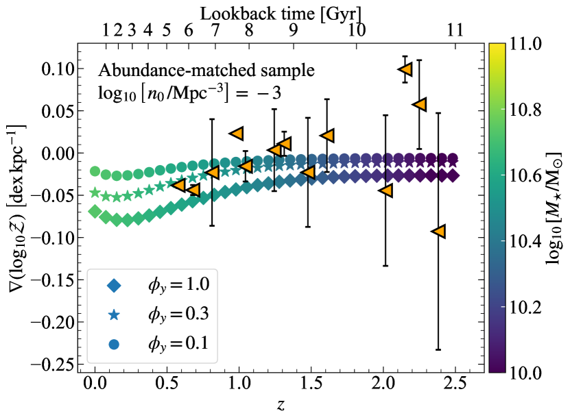
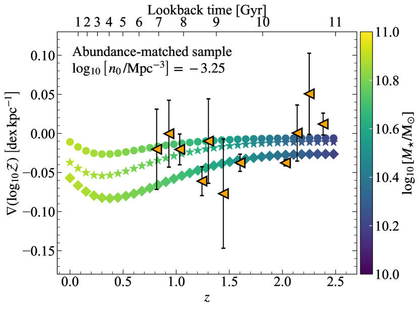
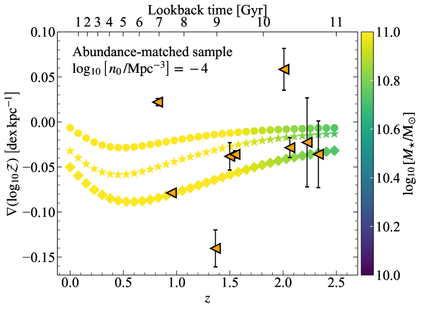
Figure 12: Trends in metallicity gradients as a function of $z$ (and lookback time) for four different abundance-matched galaxy samples given a fixed comoving number density of galaxies, $n_{0}$, color-coded by $M_{\star}$. Abundance matching leads to the selection of more massive galaxies at lower redshifts, and can be used to collectively study gradients in local spirals and their high-$z$ progenitors. The orange data points reflect mean gradients for a constructed abundance-matched sample from available observations, which are the same as that reported in Figure 11, with errorbars representing the scatter within the data. There is considerable scatter in the data, and the sample is not entirely robust given the ex post facto construction. Nonetheless, the model matches the observations reasonably-well.

Finally, we also study the evolution of metallicity gradients across an abundance-matched sample of dark matter haloes spanning a range in $z$. Abundance-matching is based on the premise that the number density of halo progenitors should nearly remain constant across $z$ within a comoving volume in the Universe (Mo et al., 1996; Mo & Fukugita, 1996; van Dokkum et al., 2010). It has been used to study a range of properties in local galaxies together with their high-$z$ progenitors (e.g., Marchesini et al., 2009; Papovich et al., 2011; Trujillo-Gomez et al., 2011; Krumholz & Dekel, 2012; Leja et al., 2013; Read & Erkal, 2019), which is not possible with other selection criteria of galaxies (e.g., selecting galaxies with identical stellar mass, as we do in Section 4.2) as such galaxies evolve in time themselves (Conroy & Wechsler, 2009).

Abundance matching involves assigning more massive galaxies to more massive haloes at every $z$; this means selecting galaxies at each $z$ with $M_{\rm{h}}(z)$ that satisfy

$$\int^{\infty}_{M_{\mathrm{h}}(z)}n\left(M_{\mathrm{h}},z\right)dM_{\mathrm{h}}=n_{0}$$ (54)

where $n_{0}$ is the target number density, and $n\left(M_{\rm{h}},z\right)$ is the number of galaxies per unit mass per unit comoving cubic Mpc given by Mo & White (2002, equation 14) based on the Sheth & Tormen (1999) modification of the Press & Schechter (1974) formalism for the number density of haloes across $z$. Thus, using the functional form for $n$, we can deduce the required $M_{\rm{h}}$ at each $z$ that would correspond to an abundance-matched sample for a given $n_{0}$. Following Marchesini et al. (2009) and Papovich et al. (2011), we study four sets of $\log_{10}\,n_{0}/\rm{Mpc^{-3}}=-3,\,-3.325\,-3.5$ and $-4.0$, respectively. For each of these $n_{0}$, we find $v_{\phi}(z)$ and $M_{\star}(z)$ using $M_{\rm{h}}(z)$ from equation 54, and $\sigma_{g}(z)$ from equation 53. We fix $\beta=0$ for all galaxies since our choice of $n_{0}$ results in massive galaxies with $M_{\star}>10^{10}\,\rm{M_{\odot}}$ for all $0\leq z\leq 2.5$. For simplicity, we fix $f_{g,Q}=f_{g,P}=0.5$ and $\sigma_{\rm{sf}}=7\,\rm{km\,s^{-1}}$, the same as that for local spirals. Given that $f_{\rm{sf}}$ varies between 0.5 and 1 as $z$ increases, we use a cubic interpolation to vary it between $z=0$ and $4$. We also fix $\mathcal{Z}_{\rm{CGM}}=0.1$.

Figure 12 shows the cosmic evolution of gradients for an abundance-matched sample of galaxies, each panel representing a different $n_{0}$. Similar to what we have seen in prior sections, the scatter in the model is the largest at the upturn where gradients start flattening. To the best of our knowledge, there are no existing abundance-matched samples of galaxies across redshift that also contain information on metallicity gradients. However, we can construct an abundance-matched sample from the available data. We caution that constructing an abundance-matched sample from existing observations ex post facto is not as accurate as properly constructing the sample to start with. In the absence of the latter, we use our constructed sample to compare against the model to learn about the kinds of metallicity gradients that existed in progenitors of local galaxies. For this purpose, we construct our pseudo-abundance matched sample as follows: for each target value of $n_{0}$, we first select a redshift, and use equation 54 to estimate the halo mass $M_{\rm{h}}$ corresponding to the target $n_{0}$ at that redshift. We then estimate the stellar mass of that galaxy $M_{\star}$ using the stellar mass-halo mass relation of Moster et al. (2013). To construct our sample set at that redshift, we then take the data collection described in Section 4.2 and select galaxies that have stellar masses within $\pm\,0.05\,\rm{dex}$ of the $M_{\star}$ from above; this constitutes our pseudo-abundance matched sample for that redshift, from which we then measure the mean and dispersion of metallicity gradient at that redshift bin. We plot these values in Figure 12, along with model predictions of the metallicity gradient, which we compute from the halo mass and redshift as in previous sections. The data we obtain in this manner have considerable scatter (shown by the errorbars), but the general trends are reasonably well reproduced by the model. However, given the uncertainties in the procedure we are forced to use to construct the observed sample, it is wiser to regard the model points in Figure 12 as a prediction for future abundance matching measurements, rather than a rigorous comparison to existing data.

5 Limitations of the model

In this section, we describe the limitations of the model, first focusing on physical processes that we have excluded, and then discussing galaxies to which we cannot always apply our assumption of equilibrium.

5.1 Additional physics

Our model omits three possibly-important physical effects: bars, galactic fountains and long term wind recycling. With regard to the first of these, there is some evidence that gas phase metallicity gradients in the presence of bars in local spirals can be systematically shallower than those non-barred galaxies (Vila-Costas & Edmunds 1992; Zaritsky et al. 1994; Zurita et al. 2021; see, however, Sánchez-Menguiano et al. 2016, 2018). We have not included metal redistribution due to bar-driven flows, and for this reason we limit our study to gradients in the parts of a galaxy where the rotation curve slope ($\beta$) is a constant, which excludes bar-dominated regions (Bland-Hawthorn & Gerhard, 2016; Martinez-Medina et al., 2020). In fact, even if we wished to include bar-driven mixing, the galaxy formation model that we use as an input in Section 2.2 is itself not applicable in regions where the bar dominates the dynamics of the galaxy, since it does not include the effects of bar-driven torques on gas and SFR surface density profiles (Sun et al., 2018, 2020).

With regard to the second issue: we do not explicitly incorporate metal redistribution via galactic fountains (Bregman, 1980). However, the combination of an enriched $\mathcal{Z}_{\rm{CGM}}$ and low $\phi_{y}$ essentially constructs a fountain process in the model that we can exploit. Semi-analytic models where the evolution of the CGM is self-consistently followed find that the CGM plays a larger role in the evolution of galaxy metallicity as it gets enriched due to outflows (Yates et al., 2020). We also note that galactic fountains, owing to their short fall-back timescale ($\sim\,100-300\,\rm{Myr}$, Anglés-Alcázar et al. 2017) and short fall-back distance from the starting point ($\sim\,1\,\rm{kpc}$, Spitoni et al. 2008) have been shown to play an insignificant role in the metallicity evolution of the local spiral M31 (Spitoni et al. 2013; see, however, simulations by Grand et al. 2019, where fountains are thought to transport metals to the edge of the star-forming disc). Fountains possibly have a significant effect on the far outskirts of the discs, where there are few or no local sources of metals.

There is some evidence from simulations that long term wind recycling can provide metals to the disc as it re-accretes the ejected material. These simulations also show that this recycling is independent of the halo mass (Christensen et al., 2016; Tollet et al., 2019), and can be the dominant mode of accretion of cold gas at late times. However, this recycling occurs much farther out in the disc than that we consider in our work, thus, its basic features are captured within $\mathcal{Z}_{\rm{CGM}}$ in the model. Additionally, while the above simulations find long term wind recycling timescale to be of the order of a Gyr, results from the EAGLE simulations find it to be comparable to $t_{\rm{H(z)}}$ (Mitchell et al., 2020). Thus, given these findings from simulations and the lack of direct observations, it is currently difficult to determine the importance of wind recycling for metallicity gradients.

Finally, we caution that our model is intended to apply mainly to metals whose production is dominated by type II SNe, and thus where the injection rate closely follows the star formation rate. We have not attempted to model elements produced by type Ia SNe or AGB stars. This is not a substantial problem for our intended application, however, since type II SNe do dominate production of the $\alpha$ elements that are most easily observable in the gas phase (Nomoto & Leung, 2018). The one exception to this statement, where some caution is warranted, is nitrogen, to which AGB stars make a substantial contribution (Meynet & Maeder, 2002; Herwig, 2005). This matters because many of the strong-line diagnostics used at high redshift rely on the N ii $\lambda 6584$ line. While observers who rely on these diagnostics usually attempt to derive the O abundance by calibrating out variations in the N/O ratio (Pettini & Pagel 2004; Masters et al. 2016; Belfiore et al. 2017; Schaefer et al. 2020; see also, Vincenzo et al. 2016), it is nevertheless the case that variations in N abundance may influence the metallicities derived at high-$z$, and that our model does not capture this effect.

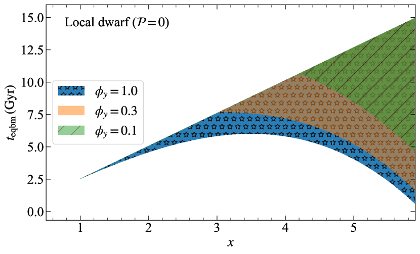
Figure 13: Same as Figure 4, but without radial inflow such that $\mathcal{P}=0$. Here, $t_{\rm{eqbm}}\gtrsim t_{\rm{H(0)}}$, implying that the metallicity gradients in such cases in local dwarfs may or may not be in equilibrium. Thus, our equilibrium model does not necessarily apply.

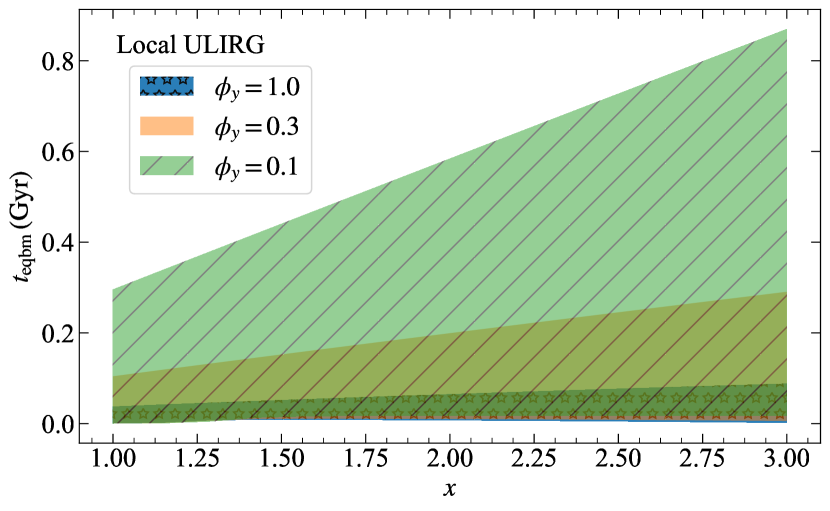
Figure 14: Same as Figure 1, but for local ultraluminous infrared galaxies (ULIRGs). Here, $t_{\rm{eqbm}}\sim t_{\rm{merge}}$, where the latter is the merger timescale of the order of $\sim\,0.3-1\,\rm{Gyr}$ as seen in models (Jiang et al., 2008; Torrey et al., 2012). Thus, the metallicity gradients may not be in equilibrium throughout the merger process. In such a case, our equilibrium model for metallicity gradients cannot be applied to local ULIRGs, and the observed gradients, if any, are transient and subject to change as the merger progresses, in line with observations (Rupke et al., 2010b; Rich et al., 2012).

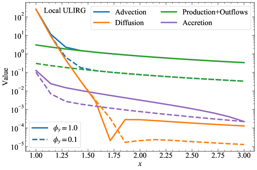
Figure 15: Same as Figure 3, but for ULIRGs, which are known to be major mergers. The non-equilibrium metallicity distribution is set by advection of gas due to tidal inflows during a merger.

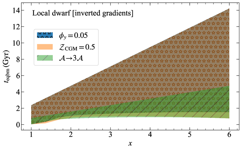
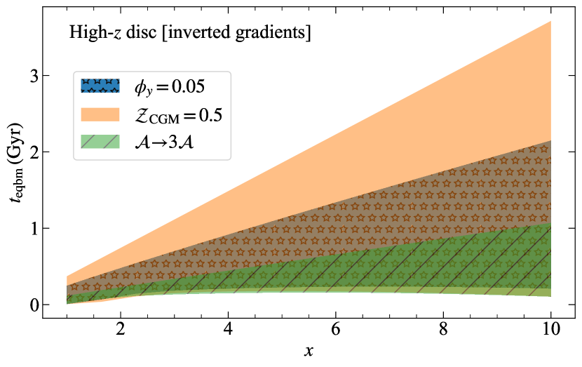
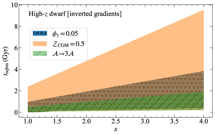
Figure 16: Metallicity equilibration timescale $t_{\rm{eqbm}}$ as a function of $x$ in galaxies with inverted gradients. The first panel represents $t_{\rm{eqbm}}$ in local dwarfs. The second panel on high-$z$ discs is identical to the class of high-$z$ galaxies we discuss in Section 3.3. The third panel plots $t_{\rm{eqbm}}$ in the case of high-$z$ dwarfs that we create by combining the fiducial parameters for local dwarfs and high-$z$ galaxies (see Section 5.2.3 for details). The colors correspond to the different ways that can give rise to an inverted gradient in a galaxy: reduction in metal yield due to high preferential metal ejection ($\phi_{y}=0.05$), enrichment of the CGM due to fountains or metal-rich flows ($\mathcal{Z}_{\rm{CGM}}=0.5$), and excessive cosmic accretion ($\mathcal{A}\to 3\mathcal{A}$). The scatter in the model is due to $c_{1}$. This plot shows that inverted metallicity gradients may or may not be in equilibrium.

5.2 Non-equilibrium metallicity gradients

There are certain classes of galaxies where we find that the metallicity distribution can be out of equilibrium, i.e., $t_{\rm{eqbm}}\gtrsim t_{\rm{H(z)}}$ or $t_{\rm{eqbm}}\gg t_{\rm{dep,H_{2}}}$. Hence, the model cannot always be used to predict metallicity gradients in such galaxies. Nonetheless, the limitation of the equilibrium model provides interesting constraints on the evolution of such galaxies. We discuss three such cases below.

5.2.1 Local dwarfs without radial inflow

The balance between metal production (source) and radial transport of metals through the disc (advection, diffusion) sets the metallicity gradients in local dwarfs (cf. Section 3.2). It has also been suggested that turbulence in these galaxies is mainly driven by star formation feedback and not gravity (Moiseev et al., 2015; Krumholz et al., 2018), which gives rise to $\sigma_{\rm{sf}}\sim\sigma_{g}$, and the low gas velocity dispersions observed in dwarfs (Yu et al., 2019; Varidel et al., 2020). Here, we investigate the case where $\sigma_{\rm{sf}}=\sigma_{g}$ such that there is no radial inflow of gas through the disc (see equation 36).

Figure 13 shows the radial profile of $t_{\rm{eqbm}}$ in this case. It is clear that $t_{\rm{eqbm}}\gtrsim t_{\rm{H(0)}}$ and $t_{\rm{eqbm}}\gtrsim t_{\rm{dep,H_{2}}}$, especially at low $\phi_{y}$, however, the exact values are sensitive to the choice of $c_{1}$. The reason for long metal equilibration timescales in this case is that, in the absence of advection, only diffusion and accretion are available to balance the source term. However, diffusion is weak due to the low gas dispersion ($\kappa_{0}\Sigma_{g0}\propto\sigma^{3}_{g}$), and accretion is weak due to the low halo mass ($\dot{\Sigma}_{\rm{cos}0}\propto M^{1.1}_{\rm{h}}$). Thus, metallicity gradients may not attain equilibrium in the absence of radial gas inflows in local dwarfs, whereas even a small amount of advection is sufficient to restore metallicity equilibrium (cf. Figure 4). In the case where there is no accretion, one can expect a diverse range of metallicity gradients that are not constrained by the model. Therefore, caution must be exercised while studying metallicity gradients in such dwarfs with an equilibrium model.

At face value, this result might seem consistent with that of Forbes et al. (2014b), where the authors find that dwarf galaxies do not attain statistical equilibrium within a Hubble time (see their Figure 15; see also, Feldmann 2015; Dashyan & Dubois 2020). However, the equilibrium scenarios considered by Forbes et al. and us are not necessarily the same, and one is not a precondition of the other. Forbes et al. discuss the equilibrium for the total amount of gas or metals in a galaxy, which is a balance between inflow and outflow. The time required to reach this equilibrium is not necessarily the same as the time to equilibrate the distribution of metals within the galactic disc, for a given total metal content. Thus, one equilibrium time can be longer or shorter than the other.

Similarly, comparing $t_{\rm{eqbm}}$ with the metal correlation timescale for local dwarfs from Krumholz & Ting (2018), which is the time required for diffusion alone to smooth out the metallicity distribution in the azimuthal direction, reveals that azimuthal metal distribution in these galaxies reaches equilibrium substantially more quickly than the radial distribution that we study here. This is consistent with the findings of Petit et al. (2015), who also find that metal distributions equilibrate much more quickly in the azimuthal than the radial direction.

5.2.2 Local ULIRGs

Local ULIRGs are very dynamically active, and are well-known to be undergoing major mergers or have companions (Lawrence et al., 1989; Melnick & Mirabel, 1990; Leech et al., 1994; Clements et al., 1996; Veilleux et al., 1999). These galaxies are often characterized by strong starburst and/or AGN-driven outflows (Veilleux et al., 1995; Veilleux et al., 2013; Soto et al., 2012; Arribas et al., 2014). They also have extremely short orbital timescales (of the order of $\sim\,5\,\mathrm{Myr}$, Krumholz et al. 2018). Local ULIRGs are very compact, with discs extending out only to $2$–$3\,\rm{kpc}$ (Downes & Solomon, 1998; Rujopakarn et al., 2011). It is quite challenging to extract gas metallicities in these galaxies because the ionised gas emission lines are often dominated by shocks (Monreal-Ibero et al., 2006, 2010) and AGN activity (Ellison et al., 2013), which interfere with traditional photoionisation-based metallicity diagnostics. In addition, high levels of dust obscuration make it difficult to model the emission line spectra (García-Marín et al., 2009; Nagao et al., 2011; Piqueras López et al., 2013; Stierwalt et al., 2014). For these reasons, there are only a handful of studies that have been able to extract gas metallicities in local ULIRGs (e.g., Kewley et al. 2006; Monreal-Ibero et al. 2007; Arribas et al. 2008; Rupke et al. 2008; Westmoquette et al. 2012; Kilerci Eser et al. 2014; Pereira-Santaella et al. 2017), and to the best our knowledge the only published studies of the metallicity gradient in ULIRGs are those of Rich et al. (2012, see their Figure 2) and Thorp et al. (2019).

The short orbital timescales of ULIRGs ensure that they return to dynamical equilibrium quickly compared to their merger timescales, which based on simulations are estimated to be $t_{\rm{merge}}\sim 0.3-1\,\rm{Gyr}$ (Jiang et al., 2008; Torrey et al., 2012). Thus our dynamical equilibrium model from Krumholz et al. (2018) is applicable to them. We investigate whether the metallicity distribution is also in equilibrium in Figure 14, which shows $t_{\rm{eqbm}}$ for local ULIRGs. It is clear that $t_{\rm{eqbm}}\sim t_{\rm{merge}}$, thus, metallicity may or may not be in equilibrium during the entire process of a merger. Our results corroborate those of Davé et al. (2012), who argue that merging galaxies should not be in equilibrium because tidal flows will fuel star formation (Barton et al., 2000; Kewley et al., 2006; Reichard et al., 2009; Perez et al., 2011; Ellison et al., 2013; Moreno et al., 2020), making cosmic accretion irrelevant. We show this quantitatively in Figure 15, where advection (radial transport of gas due to tidal inflows) is the dominant term that sets the non-equilibrium metallicity distribution, and cosmic accretion is insignificant in comparison. Our results are also in line with those from simulations and observations where metallicity gradients in local ULIRGs are observed to continuously evolve and flatten as the merger progresses (Rich et al., 2012, Figure 4), implying that the metallicity distribution is not in a steady-state. This also implies that non-equilibrium gradients in local ULIRGs are transient; assuming the galaxy settles back to being a quiescent disc after the merger, the metallicity gradient will return to the equilibrium value for a spiral galaxy on the $\sim$ few Gyr equilibrium timescale for local spirals (cf. Figure 1).

Given a merger rate, we can estimate the fraction of galaxies as a function of redshift that are expected to be out of metal equilibrium as $1-e^{-\theta}$, where $\theta$ is the product of the merger rate and the metallicity equilibration timescale. Following Rodriguez-Gomez et al. (2015, Figure 9), we see that the observed average merger rate for massive galaxies ($M_{\star}\geq 10^{10}\,\rm{M_{\odot}}$) at $z=0$ is less than $0.06\,\rm{Gyr^{-1}}$ (Lotz et al., 2011), so we expect less than 20 per cent of massive galaxies to be out of metal equilibrium at redshift zero. Similarly, based on available observational results that find a merger rate of $0.5\,\rm{Gyr^{-1}}$ at $z\approx 2$ (Bluck et al., 2009, 2012; Man et al., 2012), we expect less than 40 per cent of the most massive galaxies ($M_{\star}\geq 10^{11}\,\rm{M_{\odot}}$) to be out of metal equilibrium at redshift two. The larger fraction of galaxies that are expected to be out of metal equilibrium at high redshift could explain the inverted gradients seen in high-$z$ observations, a topic we explore in Section 5.2.3.

5.2.3 Galaxies with inverted gradients

Recent observations have discovered the presence of inverted (positive) gas phase metallicity gradients in galaxies (Sánchez et al., 2014; Belfiore et al., 2017; Mingozzi et al., 2020), especially at high redshift (Cresci et al., 2010; Queyrel et al., 2012; Stott et al., 2014; Carton et al., 2018; Wang et al., 2019; Curti et al., 2020; Wang et al., 2020; Simons et al., 2020). Inverted gradients reflect the possibility of galaxies deviating from the classical, inside-out formation picture, at least temporarily. The three leading mechanisms that are believed to give rise to an inverted gradient are: (1.) substantial metal mass loading or merger-induced tidal flows of metal-poor gas that deprives the galaxy centre of metals, especially in dwarfs (Kereš et al. 2005; Kewley et al. 2006; Emerick et al. 2018; Emerick et al. 2019; Chisholm et al. 2018; Tissera et al. 2019; see, however, Wilson et al. 2019), (2.) re-accretion of ejected metals at the outer edge of the disc from the CGM through cold, metal-rich flows or galactic fountains (Birnboim & Dekel, 2003; Dekel & Birnboim, 2006; Dekel et al., 2009a; Cresci et al., 2010; Crighton et al., 2013; Suresh et al., 2015), and (3.) cosmic accretion of metal-poor gas at the centre that dilutes the central metallicity (Cresci et al., 2010).

Corresponding to these three scenarios, we can produce inverted gradients in our model by coupling a moderate or high value of $\mathcal{Z}_{\rm GCM}$ (i.e., addition of metal-rich gas to galaxy outskirts) with small values of $\phi_{y}$ or large values of $\mathcal{A}$ (corresponding to depressed central metallicity due to heavy metal loss or rapid dilution by metal-poor gas, respectively). However, any inverted gradients that we get from the model are sensitive to our choice of $\mathcal{Z}_{\rm{CGM}}$, in the sense that we never get an inverted gradient for a sufficiently low value of $\mathcal{Z}_{\rm{CGM}}$. Nevertheless, regardless of the value of $\mathcal{Z}_{\rm{CGM}}$ that we adopt, the resulting inverted gradients may or may not be in equilibrium. We illustrate this in Figure 16, where we plot $t_{\mathrm{eqbm}}$ for local dwarfs, high-$z$ discs (identical to high-$z$ galaxies we discuss in Section 3.3), and high-$z$ dwarfs. We introduce the latter category by combining fiducial parameters for local dwarfs and high-$z$ galaxies from Table 2 in the following manner: $\beta=0.5,\,\sigma_{\mathrm{sf}}=7\,\mathrm{km\,s^{-1}},\,\sigma_{g}=40\,\mathrm{km\,s^{-1}},\,v_{\phi}=80\,\mathrm{km\,s^{-1}},f_{g,Q}=f_{g,P}=0.9,f_{\mathrm{sf}}=0.4$, and $x_{\rm{max}}=4$ at $z=2$. The three colors in all the panels in Figure 16 correspond to low $\phi_{y}=0.05$ (with $\mathcal{Z}_{\rm{CGM}}=0.1$), high $\mathcal{Z}_{\rm{CGM}}=0.5$ (with $\phi_{y}=0.1$), and high accretion where we multiply our fiducial values of $\mathcal{A}$ by 3 (with $\phi_{y}=0.1,\,\mathcal{Z}_{\rm{CGM}}=0.1$), respectively. The shaded regions correspond to the allowed values of $c_{1}$ based on the constraints we introduced in Section 2.3.

We see that whether galaxies with inverted gradients are likely to be in equilibrium or not depends largely on what produces the inversion. Galaxies where the gradient inverts due to rapid accretion (high $\mathcal{A}$) have relatively short values of $t_{\rm eqbm}$, and may be in equilibrium as long as the accretion lasts, while those that invert due to an influx of metal-rich gas at their outskirts (high $\mathcal{Z}_{\rm GCM}$) are almost certainly out of equilibrium; galaxies with extremely efficient metal loss (low $\phi_{y}$) are intermediate, and may or may not be in equilibrium. Regardless of these details, the fact that many inverted gradients are not in equilibrium also hints at the possibility of them being transient (see also, Schönrich & McMillan, 2017). This is because subsequent star formation in the galaxy centre (due to cold gas accretion or re-accretion of enriched gas from the CGM) will replenish the metal supply on timescales comparable to the star formation timescale, thus leading to the formation of a negative gradient again. Hence, we expect inverted gradients to be erased within a star formation timescale ($\lesssim 2\,\rm{Gyr}$ for massive galaxies, Leroy et al. 2008) unless they are re-established on a similar timescale. Since the processes that can cause inverted gradients (strong fountains, mergers, sudden accretion events, etc.) tend to wane with redshift, we expect that most massive galaxies will establish negative gradients by $z=0$, though some dwarfs, which have longer equilibration (and star formation) timescales, might retain their inverted gradients to $z=0$ or close to it.

6 Conclusions

In this work, we present a new theoretical model to explain the occurrence and diversity of gas phase metallicity gradients in galaxies. Starting from the conservation of metal mass, we incorporate major physical processes that can impact the distribution of metals in galaxies, namely, metal production, consumption, loss, advection, accretion and diffusion. Our first-principles based model shows that the radial metallicity gradients observed in galaxies are a natural consequence of inside-out galaxy formation. The equilibrium metallicity evolution model we present is a standalone model, but it requires inputs from a galaxy evolution model to set the galaxy properties that control metallicity. This intricate link between gas and metallicity lets us directly predict the evolution of metallicity gradients without ad hoc assumptions about galaxy properties.

The evolution of metallicities in our model depends on four dimensionless ratios: $\mathcal{T}$, $\mathcal{P}$, $\mathcal{S}$, and $\mathcal{A}$. These describe the ratio of the orbital timescale to the diffusion timescale, advection to diffusion, production (and metal ejection) to diffusion, and cosmic accretion to diffusion, respectively. Based on the input galaxy evolution model (Krumholz et al., 2018), we show how these ratios depend on various properties of the gas (cf. equation 37 $-$ equation 40). The resulting second order differential equation of the radial distribution of metallicity has a simple analytic solution given by equation 41 that we use to predict a possible range of metallicity gradients as a function of galaxy properties. We use this capability to predict the metallicity gradients of local spirals, local dwarfs, and high-redshift disc galaxies, and to predict the evolution of metallicity gradients in galaxies with redshift. Below, we list our main results:

1. The time required for the metal distribution within a galaxy to reach equilibrium is smaller than the Hubble time and comparable to the molecular gas depletion time in local spirals, (most) local dwarfs, and rotation-dominated high-$z$ galaxies. Thus, for most galaxies over most of cosmic time, the gas phase metallicity gradient is in equilibrium. Exceptions to this general trend can include merging galaxies, galaxies with inverted metallicity gradients, and some very low-mass local dwarf galaxies.

2. Galaxies tend to approach a particular value of central metallicity, dictated by the balance between the two dominant processes that depend on the properties of the galaxy (see below). The central metallicities we predict agree well with observations.

3. In local spirals, the two dominant processes shaping the metallicity gradient are metal production ($\mathcal{S}$), which tries to steepen the gradient, and accretion of metal-poor gas ($\mathcal{A}$), which tries to flatten it. On the other hand, metallicity gradients in local dwarfs and high-$z$ galaxies are set by the balance between $\mathcal{S}$ and advection of metal-poor gas from the outer to the inner parts of galaxies ($\mathcal{P}$).

4. One crucial free parameter that emerges from our model is the “yield reduction factor” $\phi_{y}$, defined as the fraction of supernova-produced metals that mix with the ISM rather than being lost immediately in metal-enhanced galactic winds. While metallicity gradients in local spirals are not tremendously sensitive to $\phi_{y}$, it has a significant effect on the metallicity gradients in local dwarfs and high-$z$ galaxies. $\phi_{y}$ also impacts the absolute metallicities in all galaxies. Comparison of the model with observations reveals that massive galaxies prefer a high value of $\phi_{y}$, whereas low-mass galaxies prefer a lower value of $\phi_{y}$. Thus, the model predicts that low-mass galaxies undergo more preferential metal ejection, and should have more metal-enriched winds than massive galaxies. Future work should thus focus on constraining $\phi_{y}$ from observations.

As a first application of our model, we study the evolution of metallicity gradients with redshift, both within a single galaxy and over samples of galaxies at different redshifts selected to have matching stellar masses or comoving densities. Our model shows that gradients in Milky Way-like galaxies have steepened over time, in qualitative agreement with recent observations; quantitative agreement between the model and the data requires a scaling of $\phi_{y}$ such that $\phi_{y}$ was low for the Galaxy in the past as compared to today, consistent with that seen in simulations. We also predict the existence of specific signatures for the evolution of metallicity gradient with redshift as a function of stellar mass that can be tested with future surveys. We show that both the Milky Way in particular and disc galaxies in general transition from the advection-dominated ($\mathcal{P}>\mathcal{A}$) to the accretion-dominated ($\mathcal{P}<\mathcal{A}$) regime from high to low redshifts. This transition mirrors the transition from gravity-driven to star formation-driven turbulence from high to low redshifts (Krumholz et al., 2018). In companion papers, we show that this transition (along with $\phi_{y}$) is also responsible for driving the shape of the mass-metallicity relation and the mass-metallicity gradient relation (Sharda et al., 2021a) in the local Universe, and we also apply our model to explain the relationship between metallicity gradients and gas kinematics in high redshift galaxies (Sharda et al., 2021b).

Data availability statement

No data were generated for this work.

Appendix A Functional form of cosmic accretion rate surface density

Here, we describe how the solutions change if we pick a different functional form for the radial profile of cosmological accretion, $\dot{c}_{\star}(x)$. Note that we must numerically solve for these functional forms, because analytic solutions either do not exist or are so complex in functional form that a numerical integration is preferable. Specifically, we experiment with $\dot{c}_{\star}(x)=1/x$ and $\dot{c}_{\star}(x)=1$.

Figure 17, Figure 18, and Figure 19 show metallicity profiles with different $\dot{c}_{\star}(x)$ for local spirals, local dwarfs, and high-$z$ galaxies with $\phi_{y}=1$, respectively; we use $\phi_{y}=1$ because this maximises the dependence on $\dot{c}_{\star}(x)$ – smaller $\phi_{y}$ values suppress variations. Note that the dimensionless parameters $\mathcal{P}$ and $\mathcal{S}$ are identical to that used in the Section 3 for the corresponding galaxies, but that $\mathcal{A}$ differs due to its dependence on $\dot{c}_{\star}$ (equation 40). We see that changing the profile of $\dot{c}_{\star}(x)$ has no noticeable effect for local dwarfs or high$-z$ galaxies. This is because cosmic accretion is not a dominant term in the metallicity model for these galaxies, and the metallicities are instead mainly set by source, advection and diffusion.

The profile of $\dot{c}_{\star}(x)$ does matter for local spirals; as $\dot{c}_{\star}(x)$ flattens, metallicities in the inner regions of the disc reach higher values whereas the outer regions of the disc become more metal poor, thus leading to somewhat steeper gradients. For the most extreme case of constant $\dot{c}_{\star}(x)$, gradients are $\approx-0.05$ dex kpc^-1 steeper than our fiducial model. Thus, if the cosmic accretion profiles in local spirals are flatter than that we use in the main text, we expect slightly steeper gradients from the metallicity model, which is largely due to the SFR that we input from the galaxy evolution model. This is because under the input galaxy evolution model of Krumholz et al. (2018) where the SFR varies as $1/x^{2}$, flatter accretion profiles will dilute the metallicity in the metal-deficient outer regions by the same amount as that in the metal-rich inner regions, thus giving a larger difference between metallicities in the inner and outer regions in the disc.

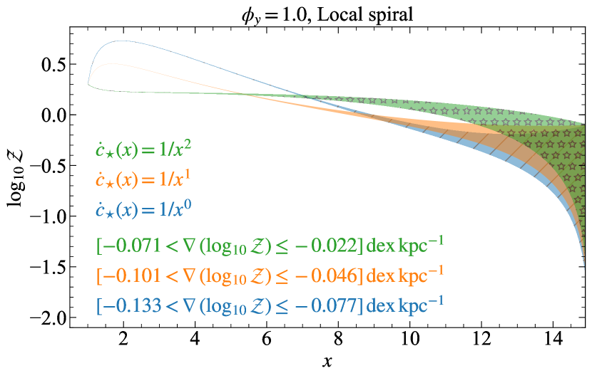
Figure 17: Same as Figure 2 but with different functional forms for cosmic accretion, namely, $\dot{c}_{\star}=1/x^{2}$ (the one we use in the main text), $1/x$ and $1$, respectively. Flatter cosmic accretion profiles make the gradients steeper (within a factor of 2).

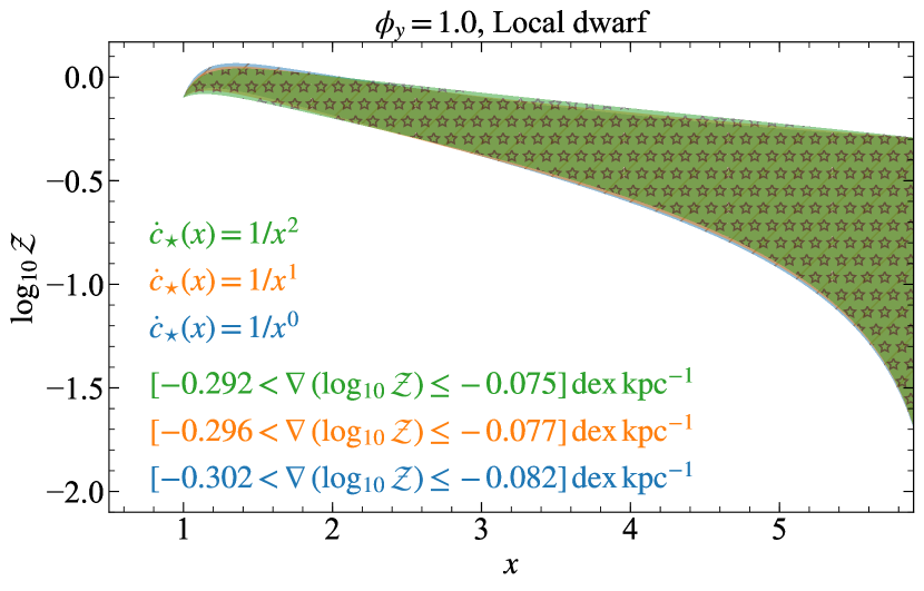
Figure 18: Same as Figure 17 but for local dwarfs. Changing the functional form of $\dot{c}_{\star}(x)$ has no impact on the metallicity distributions in local dwarfs.

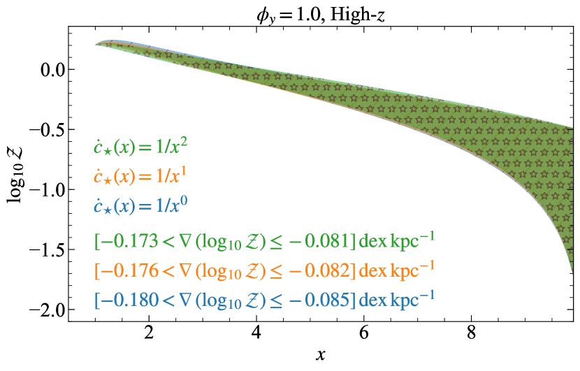
Figure 19: Same as Figure 17 but for high-$z$ galaxies. Similar to local dwarfs, changing the functional form of $\dot{c}_{\star}(x)$ has no impact on the metallicity distributions in high-$z$ galaxies.

Appendix B Uncertainties in cosmological evolution of accretion and velocity dispersion

Our predictions of metallicity gradient evolution depend on a scaling of $\sigma_{g}$ with $z$ derived from high-$z$ galaxy observations (Wisnioski et al., 2015), and a scaling of $\dot{M}_{\rm{h}}$ with $z$ derived from cosmological simulations (Neistein & Dekel, 2008; Faucher-Giguère et al., 2011). Since these two methods of deriving the scaling are very different, it is important to comment on any possible discrepancies between the two, and if they affect our results. Indeed, there is what appears at first glance to be an inconsistency: as we noted in Section 2.2, cosmological equilibrium demands that the inflow rate $\dot{M}$ through the disc (and, the star formation rate $\dot{M}_{\star}$) be similar to or less than the accretion rate onto the galaxy $\dot{M}_{\rm{ext}}$, in order to conserve the total mass. In terms of our model, the above condition translates into $\mathcal{P}/\mathcal{A}\lesssim\ln x_{\rm{max}}$ for $\dot{c}_{\star}=1/x^{2}$. However, in many cases, our adopted scalings of $\sigma_{g}$ and $\dot{M}_{h}$ with $z$ give considerably larger values of $\mathcal{P}/\mathcal{A}$ at high-$z$. This discrepancy is simply a manifestation of the known problem that galaxies at $z\sim 2$ have star formation rates $\dot{M}_{\star}>\dot{M}_{\rm{ext}}$ (Erb, 2008; Behroozi et al., 2013; Scoville et al., 2017); high-$z$ galaxies obey the same observed scaling between star formation rate and velocity dispersion as local galaxies (Krumholz et al., 2018; Varidel et al., 2020), and since the inflow rate is directly set by $\sigma_{g}$, $\dot{M}_{*}>\dot{M}_{\rm{ext}}$ directly implies $\dot{M}>\dot{M}_{\rm ext}$.

The discrepancy between star formation rates (and velocity dispersions) and expected cosmological accretion rates has several possible explanations, but from the standpoint of our model for metallicity gradients, we can divide these into two main categories. One is that galaxies near the epoch of peak star formation do in fact form stars and move mass inward faster than their mean cosmological accretion rates, either because mass that was ejected at an earlier epoch falls back onto the galactic outskirts (e.g., Christensen et al., 2016; Tollet et al., 2019), or because of large angular momentum mismatch between the infalling material and the disc that triggers a sufficiently large radial inflow (Mayor & Vigroux, 1981; Bilitewski & Schönrich, 2012; Pezzulli & Fraternali, 2016), or because galaxies accumulate large gas reservoirs at $z\gtrsim 2$, which then flow into the star-forming portion of the disc due to compaction events (Dekel et al., 2009b; Dekel & Burkert, 2014), interactions (Rupke et al., 2010a) or mergers (Hani et al., 2018) at $z\sim 2$. In these cases, the model we present is sufficient and we do not need to make any changes, since in such cases galaxies can maintain a large $\mathcal{P}/\mathcal{A}$ for a considerable time.

The other possibility is that the $\dot{M}_{\star}$ measured at high-$z$ are overestimated (e.g., Leja et al. 2019; Leja et al. 2020), thus altering the $\sigma_{g}-\dot{M}_{*}$ relationship; this is functionally equivalent to overestimating $\sigma_{g}$ at fixed $\dot{M}_{\star}$. Such an overestimate in high-redshift galaxies could plausibly be due to beam smearing, inclination uncertainty, and similar resolution-dependent (and thus redshift-dependent) factors (Davies et al., 2011; Di Teodoro & Fraternali, 2015). This would have a significant impact on $\mathcal{P}/\mathcal{A}$ because $\mathcal{P}/\mathcal{A}\propto\sigma^{3}_{g}$. To study the effects this can have on our results, we reproduce the expected cosmic evolution of metallicity gradient for the Milky Way in the model (cf. Figure 10), but using $\sigma_{g}$ obtained from equation 53 reduced by a factor of ($1+z$), in line with the redshift scaling of the limits of spectral resolution of different instruments (McDermid et al., 2020, Figure 2.3). Figure 20 presents the resulting metallicity gradients from the model, where the maximum $\log\mathcal{P}/\mathcal{A}$ is only 0.6. The qualitative shape of the model changes slightly for $z>0.5$. However, $\phi_{y}$ remains the primary factor that drives the model gradients closer to the observed gradients across cosmic time. The main difference from our fiducial model is that steep gradients become possible at high-$z$ if $\phi_{y}$ is close to unity, because a smaller $\mathcal{P}/\mathcal{A}$ implies weaker homogenisation of the ISM by inward advection of metal-poor gas.

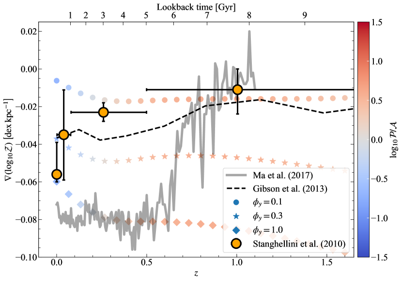
Figure 20: Same as Figure 10, but with $\sigma_{g}(z)$ reduced by a factor of $1+z$ as compared to equation 53 (see Appendix B for a discussion).

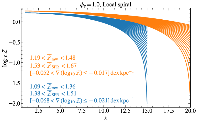
Figure 21: Metallicity gradients as shown in the main text in Section 3, but with an alternate value of the edge of the star-forming disc, $x_{\rm{max}}$. The profile of the distribution is preserved in each case, with slight variations in the absolute metallicities and metallicity gradients, with diminishing differences for decreasing $\phi_{y}$. Larger galaxies (in each galaxy class) show higher mean metallicity and flatter gradients.

Appendix C Dependence on the location of disc edges

In the main text, we non-dimensionalize the solution in terms of $x$, where $x=r/r_{0}$ and we adopt a fiducial value of $r_{0}=1\,\rm{kpc}$, finding solutions for $x$ in the range $(x_{\rm min},\,x_{\rm max})$, with $x_{\rm min}=1$ and $x_{\rm max}$ chosen based on observations of the sizes of the star-forming region for different galaxies. To explore the sensitivity of our results to the choice of our range in $x$, we show in Figure 21 how the equilibrium gradients change in local spirals if we increase $x_{\rm{max}}$ from the fiducial 15 used in the main text to 20, noting that the qualitative trends remain the same across all types of galaxies. Increasing $x_{\rm{max}}$ leads to higher metallicities at each location in the disc, with slightly higher mean metallicities and shallower metallicity gradients. This is because increasing $x_{\rm{max}}$ decreases $\mathcal{A}$ since it means that there is a larger disc for the same total cosmic accretion rate (see equation 34 and equation 40). Thus, the ratio $\mathcal{S}/\mathcal{A}$ that appears in $\mathcal{Z}$ (see equation 41) increases, giving higher $\mathcal{Z}(x)$. Further, this increment in $\mathcal{S}/\mathcal{A}$ is reduced if $\phi_{y}<1$ because $\mathcal{S}\propto\phi_{y}$. Thus, for lower $\phi_{y}$, changing $x_{\rm{max}}$ does not lead to any appreciable change in $\mathcal{Z}(x)$. Similarly, if we shift the inner edge of the galactic disc (where the rotation curve flattens out) by decreasing it to $x_{\rm{min}}=0.5$ (or increasing it to $2$), the solution allows for slightly higher (lower) mean metallicities, and steeper (shallower) gradients.

Thus, this analysis implies that in galaxies where the transition from the star-forming disc to the bulge occurs at smaller galactic radius, the galaxy could potentially build slightly steeper metallicity gradients. Conversely, in galaxies where the star-forming disc is larger, we expect slightly shallower metallicity gradients. However, these variations remain insignificant compared to the scatter introduced due to other parameters, particularly $\phi_{y}$. Thus we do not regard variations in $x_{\rm min}$ or $x_{\rm max}$ as a substantial uncertainty in the model.

References

- Acharyya et al. (2020a) Acharyya A., Krumholz M. R., Federrath C., Kewley L. J., Goldbaum N. J., Sharp R., 2020a, MNRAS, 495, 3819
- Acharyya et al. (2020b) Acharyya A., Krumholz M. R., Federrath C., Kewley L. J., Sànchez F. S., Poetrodjojo H., 2020b, MNRAS, in prep.
- Aller (1942) Aller L. H., 1942, ApJ, 95, 52
- Alves & Nelson (2000) Alves D. R., Nelson C. A., 2000, ApJ, 542, 789
- Anglés-Alcázar et al. (2017) Anglés-Alcázar D., Faucher-Giguère C.-A., Kereš D., Hopkins P. F., Quataert E., Murray N., 2017, MNRAS, 470, 4698
- Arfken (1985) Arfken G., 1985, Mathematical Methods for Physicists, third edn. Academic Press, Inc., San Diego
- Armillotta et al. (2018) Armillotta L., Krumholz M. R., Fujimoto Y., 2018, MNRAS, 481, 5000
- Arribas et al. (2008) Arribas S., Colina L., Monreal-Ibero A., Alfonso J., García-Marín M., Alonso-Herrero A., 2008, A&A, 479, 687
- Arribas et al. (2014) Arribas S., Colina L., Bellocchi E., Maiolino R., Villar-Martín M., 2014, A&A, 568, A14
- Asplund et al. (2009) Asplund M., Grevesse N., Sauval A. J., Scott P., 2009, ARA&A, 47, 481
- Astropy Collaboration et al. (2013) Astropy Collaboration et al., 2013, A&A, 558, A33
- Astropy Collaboration et al. (2018) Astropy Collaboration et al., 2018, AJ, 156, 123
- Aumer et al. (2013) Aumer M., White S. D. M., Naab T., Scannapieco C., 2013, MNRAS, 434, 3142
- Barton et al. (2000) Barton E. J., Geller M. J., Kenyon S. J., 2000, ApJ, 530, 660
- Behroozi et al. (2013) Behroozi P. S., Wechsler R. H., Conroy C., 2013, ApJ, 762, L31
- Belfiore et al. (2017) Belfiore F., et al., 2017, MNRAS, 469, 151
- Belfiore et al. (2019) Belfiore F., Vincenzo F., Maiolino R., Matteucci F., 2019, MNRAS, 487, 456
- Bellardini et al. (2021) Bellardini M. A., Wetzel A., Loebman S. R., Faucher-Giguère C.-A., Ma X., Feldmann R., 2021, arXiv e-prints, p. arXiv:2102.06220
- Benson (2010) Benson A. J., 2010, Phys. Rep., 495, 33
- Bigiel & Blitz (2012) Bigiel F., Blitz L., 2012, ApJ, 756, 183
- Bigiel et al. (2008) Bigiel F., Leroy A., Walter F., Brinks E., de Blok W. J. G., Madore B., Thornley M. D., 2008, AJ, 136, 2846
- Bilitewski & Schönrich (2012) Bilitewski T., Schönrich R., 2012, MNRAS, 426, 2266
- Birnboim & Dekel (2003) Birnboim Y., Dekel A., 2003, MNRAS, 345, 349
- Bland-Hawthorn & Gerhard (2016) Bland-Hawthorn J., Gerhard O., 2016, ARA&A, 54, 529
- Bluck et al. (2009) Bluck A. F. L., Conselice C. J., Bouwens R. J., Daddi E., Dickinson M., Papovich C., Yan H., 2009, MNRAS, 394, L51
- Bluck et al. (2012) Bluck A. F. L., Conselice C. J., Buitrago F., Grützbauch R., Hoyos C., Mortlock A., Bauer A. E., 2012, ApJ, 747, 34
- Bolatto et al. (2011) Bolatto A. D., et al., 2011, ApJ, 741, 12
- Bothwell et al. (2014) Bothwell M. S., et al., 2014, MNRAS, 445, 2599
- Bouché et al. (2010) Bouché N., et al., 2010, ApJ, 718, 1001
- Bouché et al. (2012) Bouché N., Hohensee W., Vargas R., Kacprzak G. G., Martin C. L., Cooke J., Churchill C. W., 2012, MNRAS, 426, 801
- Bregman (1980) Bregman J. N., 1980, ApJ, 236, 577
- Bresolin (2019) Bresolin F., 2019, MNRAS, 488, 3826
- Bryant et al. (2015) Bryant J. J., et al., 2015, MNRAS, 447, 2857
- Bundy et al. (2015) Bundy K., et al., 2015, ApJ, 798, 7
- Bunker et al. (2020) Bunker A. J., NIRSPEC Instrument Science Team JAESs Collaboration 2020, in da Cunha E., Hodge J., Afonso J., Pentericci L., Sobral D., eds, Vol. 352, Uncovering Early Galaxy Evolution in the ALMA and JWST Era. pp 342–346, doi:10.1017/S1743921319009463
- Burkert et al. (2010) Burkert A., et al., 2010, ApJ, 725, 2324
- Carton et al. (2015) Carton D., et al., 2015, MNRAS, 451, 210
- Carton et al. (2017) Carton D., et al., 2017, MNRAS, 468, 2140
- Carton et al. (2018) Carton D., et al., 2018, MNRAS, 478, 4293
- Cavichia et al. (2011) Cavichia O., Costa R. D. D., Maciel W. J., 2011, Rev. Mex. Astron. Astrofis., 47, 49
- Chiappini et al. (1997) Chiappini C., Matteucci F., Gratton R., 1997, ApJ, 477, 765
- Chiappini et al. (2001) Chiappini C., Matteucci F., Romano D., 2001, ApJ, 554, 1044
- Chisholm et al. (2017) Chisholm J., Tremonti C. A., Leitherer C., Chen Y., 2017, MNRAS, 469, 4831
- Chisholm et al. (2018) Chisholm J., Tremonti C., Leitherer C., 2018, MNRAS, 481, 1690
- Christensen et al. (2016) Christensen C. R., Davé R., Governato F., Pontzen A., Brooks A., Munshi F., Quinn T., Wadsley J., 2016, ApJ, 824, 57
- Christensen et al. (2018) Christensen C. R., Davé R., Brooks A., Quinn T., Shen S., 2018, ApJ, 867, 142
- Clements et al. (1996) Clements D. L., Sutherland W. J., McMahon R. G., Saunders W., 1996, MNRAS, 279, 477
- Colavitti et al. (2008) Colavitti E., Matteucci F., Murante G., 2008, A&A, 483, 401
- Collacchioni et al. (2020) Collacchioni F., Lagos C. D. P., Mitchell P. D., Schaye J., Wisnioski E., Cora S. A., Correa C. A., 2020, MNRAS, 495, 2827
- Conroy & Wechsler (2009) Conroy C., Wechsler R. H., 2009, ApJ, 696, 620
- Courty et al. (2010) Courty S., Gibson B. K., Teyssier R., 2010, in Debattista V. P., Popescu C. C., eds, American Institute of Physics Conference Series Vol. 1240, American Institute of Physics Conference Series. pp 131–134 (arXiv:1002.2383), doi:10.1063/1.3458467
- Creasey et al. (2013) Creasey P., Theuns T., Bower R. G., 2013, MNRAS, 429, 1922
- Creasey et al. (2015) Creasey P., Theuns T., Bower R. G., 2015, MNRAS, 446, 2125
- Cresci et al. (2010) Cresci G., Mannucci F., Maiolino R., Marconi A., Gnerucci A., Magrini L., 2010, Nature, 467, 811
- Crighton et al. (2013) Crighton N. H. M., Hennawi J. F., Prochaska J. X., 2013, ApJ, 776, L18
- Curti et al. (2020) Curti M., et al., 2020, MNRAS, 492, 821
- Dalcanton (2007) Dalcanton J. J., 2007, ApJ, 658, 941
- Dashyan & Dubois (2020) Dashyan G., Dubois Y., 2020, A&A, 638, A123
- Davé et al. (2011) Davé R., Finlator K., Oppenheimer B. D., 2011, MNRAS, 416, 1354
- Davé et al. (2012) Davé R., Finlator K., Oppenheimer B. D., 2012, MNRAS, 421, 98
- Davies et al. (2011) Davies R., et al., 2011, ApJ, 741, 69
- Davies et al. (2019) Davies R. L., et al., 2019, ApJ, 873, 122
- Davies et al. (2020) Davies R. L., et al., 2020, arXiv e-prints, p. arXiv:2012.10445
- Dayal et al. (2013) Dayal P., Ferrara A., Dunlop J. S., 2013, MNRAS, 430, 2891
- De Vis et al. (2019) De Vis P., et al., 2019, A&A, 623, A5
- Dekel & Birnboim (2006) Dekel A., Birnboim Y., 2006, MNRAS, 368, 2
- Dekel & Burkert (2014) Dekel A., Burkert A., 2014, MNRAS, 438, 1870
- Dekel et al. (2009a) Dekel A., et al., 2009a, Nature, 457, 451
- Dekel et al. (2009b) Dekel A., Sari R., Ceverino D., 2009b, ApJ, 703, 785
- Dekel et al. (2013) Dekel A., Zolotov A., Tweed D., Cacciato M., Ceverino D., Primack J. R., 2013, MNRAS, 435, 999
- Di Teodoro & Fraternali (2015) Di Teodoro E. M., Fraternali F., 2015, MNRAS, 451, 3021
- Di Teodoro et al. (2016) Di Teodoro E. M., Fraternali F., Miller S. H., 2016, A&A, 594, A77
- Downes & Solomon (1998) Downes D., Solomon P. M., 1998, ApJ, 507, 615
- Du et al. (2017) Du W., Wu H., Zhu Y., Zheng W., Filippenko A. V., 2017, ApJ, 837, 152
- Dutton & Macciò (2014) Dutton A. A., Macciò A. V., 2014, MNRAS, 441, 3359
- Ellison et al. (2013) Ellison S. L., Mendel J. T., Patton D. R., Scudder J. M., 2013, MNRAS, 435, 3627
- Emerick et al. (2018) Emerick A., Bryan G. L., Mac Low M.-M., Côté B., Johnston K. V., O’Shea B. W., 2018, ApJ, 869, 94
- Emerick et al. (2019) Emerick A., Bryan G. L., Mac Low M.-M., 2019, MNRAS, 482, 1304
- Erb (2008) Erb D. K., 2008, ApJ, 674, 151
- Erb et al. (2006) Erb D. K., Shapley A. E., Pettini M., Steidel C. C., Reddy N. A., Adelberger K. L., 2006, ApJ, 644, 813
- Erroz-Ferrer et al. (2019) Erroz-Ferrer S., et al., 2019, MNRAS, 484, 5009
- Faucher-Giguère (2018) Faucher-Giguère C.-A., 2018, MNRAS, 473, 3717
- Faucher-Giguère et al. (2011) Faucher-Giguère C.-A., Kereš D., Ma C.-P., 2011, MNRAS, 417, 2982
- Federrath (2013) Federrath C., 2013, MNRAS, 436, 3167
- Feldmann (2015) Feldmann R., 2015, MNRAS, 449, 3274
- Finlator & Davé (2008) Finlator K., Davé R., 2008, MNRAS, 385, 2181
- Florido et al. (2012) Florido E., Pérez I., Zurita A., Sánchez-Blázquez P., 2012, A&A, 543, A150
- Forbes et al. (2012) Forbes J., Krumholz M., Burkert A., 2012, ApJ, 754, 48
- Forbes et al. (2014a) Forbes J. C., Krumholz M. R., Burkert A., Dekel A., 2014a, MNRAS, 438, 1552
- Forbes et al. (2014b) Forbes J. C., Krumholz M. R., Burkert A., Dekel A., 2014b, MNRAS, 443, 168
- Forbes et al. (2019) Forbes J. C., Krumholz M. R., Speagle J. S., 2019, MNRAS, 487, 3581
- Förster Schreiber et al. (2009) Förster Schreiber N. M., et al., 2009, ApJ, 706, 1364
- Förster Schreiber et al. (2018) Förster Schreiber N. M., et al., 2018, ApJS, 238, 21
- Förster Schreiber et al. (2019) Förster Schreiber N. M., et al., 2019, ApJ, 875, 21
- Foster et al. (2020) Foster C., et al., 2020, arXiv e-prints, p. arXiv:2011.13567
- Freeman & Bland-Hawthorn (2002) Freeman K., Bland-Hawthorn J., 2002, ARA&A, 40, 487
- Fu et al. (2009) Fu J., Hou J. L., Yin J., Chang R. X., 2009, ApJ, 696, 668
- Fu et al. (2013) Fu J., et al., 2013, MNRAS, 434, 1531
- Furlanetto (2021) Furlanetto S. R., 2021, MNRAS, 500, 3394
- García-Marín et al. (2009) García-Marín M., Colina L., Arribas S., 2009, A&A, 505, 1017
- Geach et al. (2011) Geach J. E., Smail I., Moran S. M., MacArthur L. A., Lagos C. d. P., Edge A. C., 2011, ApJ, 730, L19
- Genel et al. (2012) Genel S., et al., 2012, ApJ, 745, 11
- Genzel et al. (2010) Genzel R., et al., 2010, MNRAS, 407, 2091
- Genzel et al. (2011) Genzel R., et al., 2011, ApJ, 733, 101
- Genzel et al. (2015) Genzel R., et al., 2015, ApJ, 800, 20
- Gibson et al. (2013) Gibson B. K., Pilkington K., Brook C. B., Stinson G. S., Bailin J., 2013, A&A, 554, A47
- Gillman et al. (2021) Gillman S., et al., 2021, MNRAS, 500, 4229
- Grand et al. (2019) Grand R. J. J., et al., 2019, MNRAS, 490, 4786
- Greif et al. (2009) Greif T. H., Glover S. C. O., Bromm V., Klessen R. S., 2009, MNRAS, 392, 1381
- Grossi et al. (2020) Grossi M., García-Benito R., Cortesi A., Gonçalves D. R., Gonçalves T. S., Lopes P. A. A., Menéndez-Delmestre K., Telles E., 2020, MNRAS, 498, 1939
- Hani et al. (2018) Hani M. H., Sparre M., Ellison S. L., Torrey P., Vogelsberger M., 2018, MNRAS, 475, 1160
- Harris et al. (2020) Harris C. R., et al., 2020, Nature, 585, 357
- Heckman et al. (1990) Heckman T. M., Armus L., Miley G. K., 1990, ApJS, 74, 833
- Hemler et al. (2020) Hemler Z. S., et al., 2020, arXiv e-prints, p. arXiv:2007.10993
- Henriques et al. (2013) Henriques B. M. B., White S. D. M., Thomas P. A., Angulo R. E., Guo Q., Lemson G., Springel V., 2013, MNRAS, 431, 3373
- Henriques et al. (2020) Henriques B. M. B., Yates R. M., Fu J., Guo Q., Kauffmann G., Srisawat C., Thomas P. A., White S. D. M., 2020, MNRAS, 491, 5795
- Herwig (2005) Herwig F., 2005, ARA&A, 43, 435
- Hillebrandt & Niemeyer (2000) Hillebrandt W., Niemeyer J. C., 2000, ARA&A, 38, 191
- Ho et al. (2015) Ho I. T., Kudritzki R.-P., Kewley L. J., Zahid H. J., Dopita M. A., Bresolin F., Rupke D. S. N., 2015, MNRAS, 448, 2030
- Hopkins et al. (2014) Hopkins P. F., Kereš D., Oñorbe J., Faucher-Giguère C.-A., Quataert E., Murray N., Bullock J. S., 2014, MNRAS, 445, 581
- Hopkins et al. (2018) Hopkins P. F., et al., 2018, MNRAS, 480, 800
- Huang & Kauffmann (2014) Huang M.-L., Kauffmann G., 2014, MNRAS, 443, 1329
- Hunt et al. (2015) Hunt L. K., et al., 2015, A&A, 583, A114
- Hunt et al. (2016) Hunt L., Dayal P., Magrini L., Ferrara A., 2016, MNRAS, 463, 2020
- Hunter (2007) Hunter J. D., 2007, Computing in Science & Engineering, 9, 90
- Inoue et al. (2016) Inoue S., Dekel A., Mandelker N., Ceverino D., Bournaud F., Primack J., 2016, MNRAS, 456, 2052
- Isbell et al. (2018) Isbell J. W., Xue R., Fu H., 2018, ApJ, 869, L37
- Jameson et al. (2016) Jameson K. E., et al., 2016, ApJ, 825, 12
- Jameson et al. (2018) Jameson K. E., et al., 2018, ApJ, 853, 111
- Jiang et al. (2008) Jiang C. Y., Jing Y. P., Faltenbacher A., Lin W. P., Li C., 2008, ApJ, 675, 1095
- Johnson et al. (2018) Johnson H. L., et al., 2018, MNRAS, 474, 5076
- Jones et al. (2013) Jones T., Ellis R. S., Richard J., Jullo E., 2013, ApJ, 765, 48
- Kaasinen et al. (2017) Kaasinen M., Bian F., Groves B., Kewley L. J., Gupta A., 2017, MNRAS, 465, 3220
- Kacprzak et al. (2014) Kacprzak G. G., et al., 2014, ApJ, 792, L12
- Kalberla & Kerp (2009) Kalberla P. M. W., Kerp J., 2009, ARA&A, 47, 27
- Kang et al. (2021) Kang X., Chang R., Kudritzki R.-P., Gong X., Zhang F., 2021, arXiv e-prints, p. arXiv:2101.06833
- Karlsson et al. (2013) Karlsson T., Bromm V., Bland-Hawthorn J., 2013, Reviews of Modern Physics, 85, 809
- Kashino et al. (2017) Kashino D., et al., 2017, ApJ, 835, 88
- Kauffmann et al. (2013) Kauffmann G., Li C., Zhang W., Weinmann S., 2013, MNRAS, 430, 1447
- Kereš et al. (2005) Kereš D., Katz N., Weinberg D. H., Davé R., 2005, MNRAS, 363, 2
- Kewley et al. (2006) Kewley L. J., Geller M. J., Barton E. J., 2006, AJ, 131, 2004
- Kewley et al. (2019a) Kewley L. J., Nicholls D. C., Sutherland R. S., 2019a, ARA&A, 57, 511
- Kewley et al. (2019b) Kewley L. J., Nicholls D. C., Sutherland R., Rigby J. R., Acharya A., Dopita M. A., Bayliss M. B., 2019b, ApJ, 880, 16
- Kilerci Eser et al. (2014) Kilerci Eser E., Goto T., Doi Y., 2014, ApJ, 797, 54
- Kim et al. (2020) Kim C.-G., et al., 2020, ApJ, 900, 61
- Kobayashi et al. (2006) Kobayashi C., Umeda H., Nomoto K., Tominaga N., Ohkubo T., 2006, ApJ, 653, 1145
- Kreyszig et al. (2011) Kreyszig E., Kreyszig H., Norminton E. J., 2011, Advanced Engineering Mathematics, tenth edn. Wiley, Hoboken, NJ, USA
- Kruijssen & Longmore (2014) Kruijssen J. M. D., Longmore S. N., 2014, MNRAS, 439, 3239
- Krumholz (2013) Krumholz M. R., 2013, MNRAS, 436, 2747
- Krumholz & Burkert (2010) Krumholz M., Burkert A., 2010, ApJ, 724, 895
- Krumholz & Dekel (2012) Krumholz M. R., Dekel A., 2012, ApJ, 753, 16
- Krumholz & McKee (2005) Krumholz M. R., McKee C. F., 2005, ApJ, 630, 250
- Krumholz & Ting (2018) Krumholz M. R., Ting Y.-S., 2018, MNRAS, 475, 2236
- Krumholz et al. (2008) Krumholz M. R., McKee C. F., Tumlinson J., 2008, ApJ, 689, 865
- Krumholz et al. (2009) Krumholz M. R., McKee C. F., Tumlinson J., 2009, ApJ, 693, 216
- Krumholz et al. (2012) Krumholz M. R., Dekel A., McKee C. F., 2012, ApJ, 745, 69
- Krumholz et al. (2018) Krumholz M. R., Burkhart B., Forbes J. C., Crocker R. M., 2018, MNRAS, 477, 2716
- Kubryk et al. (2013) Kubryk M., Prantzos N., Athanassoula E., 2013, MNRAS, 436, 1479
- Kudritzki et al. (2015) Kudritzki R.-P., Ho I. T., Schruba A., Burkert A., Zahid H. J., Bresolin F., Dima G. I., 2015, MNRAS, 450, 342
- Lawrence et al. (1989) Lawrence A., Rowan-Robinson M., Leech K., Jones D. H. P., Wall J. V., 1989, MNRAS, 240, 329
- Leech et al. (1994) Leech K. J., Rowan-Robinson M., Lawrence A., Hughes J. D., 1994, MNRAS, 267, 253
- Leethochawalit et al. (2016) Leethochawalit N., Jones T. A., Ellis R. S., Stark D. P., Richard J., Zitrin A., Auger M., 2016, ApJ, 820, 84
- Leitner & Kravtsov (2011) Leitner S. N., Kravtsov A. V., 2011, ApJ, 734, 48
- Leja et al. (2013) Leja J., van Dokkum P., Franx M., 2013, ApJ, 766, 33
- Leja et al. (2019) Leja J., et al., 2019, ApJ, 877, 140
- Leja et al. (2020) Leja J., Speagle J. S., Johnson B. D., Conroy C., van Dokkum P., Franx M., 2020, ApJ, 893, 111
- Leroy et al. (2008) Leroy A. K., Walter F., Brinks E., Bigiel F., de Blok W. J. G., Madore B., Thornley M. D., 2008, AJ, 136, 2782
- Leroy et al. (2013) Leroy A. K., et al., 2013, AJ, 146, 19
- Lilly et al. (2013) Lilly S. J., Carollo C. M., Pipino A., Renzini A., Peng Y., 2013, ApJ, 772, 119
- Lotz et al. (2011) Lotz J. M., Jonsson P., Cox T. J., Croton D., Primack J. R., Somerville R. S., Stewart K., 2011, ApJ, 742, 103
- Ma et al. (2017) Ma X., Hopkins P. F., Feldmann R., Torrey P., Faucher-Giguère C.-A., Kereš D., 2017, MNRAS, 466, 4780
- Mac Low & Ferrara (1999) Mac Low M.-M., Ferrara A., 1999, ApJ, 513, 142
- Macciò et al. (2007) Macciò A. V., Dutton A. A., van den Bosch F. C., Moore B., Potter D., Stadel J., 2007, MNRAS, 378, 55
- Maciel & Costa (2013) Maciel W. J., Costa R. D. D., 2013, Rev. Mex. Astron. Astrofis., 49, 333
- Maciel et al. (2003) Maciel W. J., Costa R. D. D., Uchida M. M. M., 2003, A&A, 397, 667
- Maciel et al. (2010) Maciel W. J., Costa R. D. D., Idiart T. E. P., 2010, A&A, 512, A19
- Magrini et al. (2016) Magrini L., Coccato L., Stanghellini L., Casasola V., Galli D., 2016, A&A, 588, A91
- Maiolino & Mannucci (2019) Maiolino R., Mannucci F., 2019, A&ARv, 27, 3
- Maiolino et al. (2008) Maiolino R., et al., 2008, A&A, 488, 463
- Man et al. (2012) Man A. W. S., Toft S., Zirm A. W., Wuyts S., van der Wel A., 2012, ApJ, 744, 85
- Marchesini et al. (2009) Marchesini D., van Dokkum P. G., Förster Schreiber N. M., Franx M., Labbé I., Wuyts S., 2009, ApJ, 701, 1765
- Marconi et al. (1994) Marconi G., Matteucci F., Tosi M., 1994, MNRAS, 270, 35
- Martin & Kennicutt (2001) Martin C. L., Kennicutt Robert C. J., 2001, ApJ, 555, 301
- Martin et al. (2002) Martin C. L., Kobulnicky H. A., Heckman T. M., 2002, ApJ, 574, 663
- Martinez-Medina et al. (2020) Martinez-Medina L. A., Pichardo B., Peimbert A., 2020, MNRAS, 496, 1845
- Mast et al. (2014) Mast D., et al., 2014, A&A, 561, A129
- Masters et al. (2016) Masters D., Faisst A., Capak P., 2016, ApJ, 828, 18
- Mayor & Vigroux (1981) Mayor M., Vigroux L., 1981, A&A, 98, 1
- McDermid et al. (2020) McDermid R. M., et al., 2020, arXiv e-prints, p. arXiv:2009.09242
- McKee et al. (2015) McKee C. F., Parravano A., Hollenbach D. J., 2015, ApJ, 814, 13
- McQuinn et al. (2019) McQuinn K. B. W., van Zee L., Skillman E. D., 2019, ApJ, 886, 74
- Melnick & Mirabel (1990) Melnick J., Mirabel I. F., 1990, A&A, 231, L19
- Meurer et al. (2013) Meurer G. R., Zheng Z., de Blok W. J. G., 2013, MNRAS, 429, 2537
- Meynet & Maeder (2002) Meynet G., Maeder A., 2002, A&A, 381, L25
- Minchev et al. (2013) Minchev I., Chiappini C., Martig M., 2013, A&A, 558, A9
- Mingozzi et al. (2020) Mingozzi M., et al., 2020, A&A, 636, A42
- Mitchell et al. (2020) Mitchell P. D., Schaye J., Bower R. G., 2020, MNRAS, 497, 4495
- Mo & Fukugita (1996) Mo H. J., Fukugita M., 1996, ApJ, 467, L9
- Mo & White (2002) Mo H. J., White S. D. M., 2002, MNRAS, 336, 112
- Mo et al. (1996) Mo H. J., Jing Y. P., White S. D. M., 1996, MNRAS, 282, 1096
- Mo et al. (2010) Mo H., van den Bosch F. C., White S., 2010, Galaxy Formation and Evolution. Cambridge University Press
- Moiseev et al. (2015) Moiseev A. V., Tikhonov A. V., Klypin A., 2015, MNRAS, 449, 3568
- Molina et al. (2017) Molina J., Ibar E., Swinbank A. M., Sobral D., Best P. N., Smail I., Escala A., Cirasuolo M., 2017, MNRAS, 466, 892
- Mollá & Díaz (2005) Mollá M., Díaz A. I., 2005, MNRAS, 358, 521
- Mollá et al. (2016) Mollá M., Díaz Á. I., Gibson B. K., Cavichia O., López-Sánchez Á.-R., 2016, MNRAS, 462, 1329
- Mollá et al. (2019) Mollá M., Díaz Á. I., Cavichia O., Gibson B. K., Maciel W. J., Costa R. D. D., Ascasibar Y., Few C. G., 2019, MNRAS, 482, 3071
- Monreal-Ibero et al. (2006) Monreal-Ibero A., Arribas S., Colina L., 2006, ApJ, 637, 138
- Monreal-Ibero et al. (2007) Monreal-Ibero A., Colina L., Arribas S., García-Marín M., 2007, A&A, 472, 421
- Monreal-Ibero et al. (2010) Monreal-Ibero A., Arribas S., Colina L., Rodríguez-Zaurín J., Alonso-Herrero A., García-Marín M., 2010, A&A, 517, A28
- Moran et al. (2012) Moran S. M., et al., 2012, ApJ, 745, 66
- Moreno et al. (2020) Moreno J., et al., 2020, MNRAS, tmp
- Morokuma-Matsui & Baba (2015) Morokuma-Matsui K., Baba J., 2015, MNRAS, 454, 3792
- Moster et al. (2010) Moster B. P., Somerville R. S., Maulbetsch C., van den Bosch F. C., Macciò A. V., Naab T., Oser L., 2010, ApJ, 710, 903
- Moster et al. (2013) Moster B. P., Naab T., White S. D. M., 2013, MNRAS, 428, 3121
- Mott et al. (2013) Mott A., Spitoni E., Matteucci F., 2013, MNRAS, 435, 2918
- Moustakas et al. (2010) Moustakas J., Kennicutt Robert C. J., Tremonti C. A., Dale D. A., Smith J.-D. T., Calzetti D., 2010, ApJS, 190, 233
- Muratov et al. (2015) Muratov A. L., Kereš D., Faucher-Giguère C.-A., Hopkins P. F., Quataert E., Murray N., 2015, MNRAS, 454, 2691
- Nagao et al. (2011) Nagao T., Maiolino R., Marconi A., Matsuhara H., 2011, A&A, 526, A149
- Navarro et al. (1997) Navarro J. F., Frenk C. S., White S. D. M., 1997, ApJ, 490, 493
- Neistein & Dekel (2008) Neistein E., Dekel A., 2008, MNRAS, 383, 615
- Newman et al. (2012) Newman S. F., et al., 2012, ApJ, 761, 43
- Nomoto & Leung (2018) Nomoto K., Leung S.-C., 2018, Space Sci. Rev., 214, 67
- Oliphant (2006) Oliphant T. E., 2006, A guide to NumPy. Vol. 1, Trelgol Publishing USA
- Onodera et al. (2016) Onodera M., et al., 2016, ApJ, 822, 42
- Oppenheimer et al. (2010) Oppenheimer B. D., Davé R., Kereš D., Fardal M., Katz N., Kollmeier J. A., Weinberg D. H., 2010, MNRAS, 406, 2325
- Origlia et al. (2004) Origlia L., Ranalli P., Comastri A., Maiolino R., 2004, ApJ, 606, 862
- Pace et al. (2020) Pace Z. J., Tremonti C., Schaefer A. L., Stark D. V., Witherspoon C. A., Masters K. L., Drory N., Zhang K., 2020, arXiv e-prints, p. arXiv:2012.12887
- Pagel & Patchett (1975) Pagel B. E. J., Patchett B. E., 1975, MNRAS, 172, 13
- Pandya et al. (2020) Pandya V., et al., 2020, ApJ, 905, 4
- Papovich et al. (2011) Papovich C., Finkelstein S. L., Ferguson H. C., Lotz J. M., Giavalisco M., 2011, MNRAS, 412, 1123
- Patankar (1980) Patankar S. V., 1980, Numerical heat transfer and fluid flow. Series on Computational Methods in Mechanics and Thermal Science, Hemisphere Publishing Corporation (CRC Press, Taylor & Francis Group), http://www.crcpress.com/product/isbn/9780891165224
- Peeples & Shankar (2011) Peeples M. S., Shankar F., 2011, MNRAS, 417, 2962
- Pereira-Santaella et al. (2017) Pereira-Santaella M., Rigopoulou D., Farrah D., Lebouteiller V., Li J., 2017, MNRAS, 470, 1218
- Perez et al. (2011) Perez J., Michel-Dansac L., Tissera P. B., 2011, MNRAS, 417, 580
- Petit et al. (2015) Petit A. C., Krumholz M. R., Goldbaum N. J., Forbes J. C., 2015, MNRAS, 449, 2588
- Pettini & Pagel (2004) Pettini M., Pagel B. E. J., 2004, MNRAS, 348, L59
- Pezzulli & Fraternali (2016) Pezzulli G., Fraternali F., 2016, MNRAS, 455, 2308
- Pilkington et al. (2012) Pilkington K., et al., 2012, A&A, 540, A56
- Pillepich et al. (2019) Pillepich A., et al., 2019, MNRAS, 490, 3196
- Pilyugin (1993) Pilyugin L. S., 1993, A&A, 277, 42
- Piqueras López et al. (2013) Piqueras López J., Colina L., Arribas S., Alonso-Herrero A., 2013, A&A, 553, A85
- Planck Collaboration et al. (2016) Planck Collaboration et al., 2016, A&A, 594, A13
- Planck Collaboration et al. (2018) Planck Collaboration et al., 2018, arXiv e-prints, p. arXiv:1807.06209
- Poetrodjojo et al. (2019) Poetrodjojo H., D’Agostino J. J., Groves B., Kewley L., Ho I. T., Rich J., Madore B. F., Seibert M., 2019, MNRAS, 487, 79
- Poetrodjojo et al. (2021) Poetrodjojo H., et al., 2021, MNRAS, tmp
- Prantzos & Boissier (2000) Prantzos N., Boissier S., 2000, MNRAS, 313, 338
- Press & Schechter (1974) Press W. H., Schechter P., 1974, ApJ, 187, 425
- Prochaska et al. (2017) Prochaska J. X., et al., 2017, ApJ, 837, 169
- Queyrel et al. (2012) Queyrel J., et al., 2012, A&A, 539, A93
- Read & Erkal (2019) Read J. I., Erkal D., 2019, MNRAS, 487, 5799
- Recchi et al. (2001) Recchi S., Matteucci F., D’Ercole A., 2001, MNRAS, 322, 800
- Recchi et al. (2008) Recchi S., Spitoni E., Matteucci F., Lanfranchi G. A., 2008, A&A, 489, 555
- Reichard et al. (2009) Reichard T. A., Heckman T. M., Rudnick G., Brinchmann J., Kauffmann G., Wild V., 2009, ApJ, 691, 1005
- Rennehan et al. (2019) Rennehan D., Babul A., Hopkins P. F., Davé R., Moa B., 2019, MNRAS, 483, 3810
- Rich et al. (2012) Rich J. A., Torrey P., Kewley L. J., Dopita M. A., Rupke D. S. N., 2012, ApJ, 753, 5
- Robles-Valdez et al. (2017) Robles-Valdez F., Rodríguez-González A., Hernández-Martínez L., Esquivel A., 2017, ApJ, 835, 136
- Rodriguez-Gomez et al. (2015) Rodriguez-Gomez V., et al., 2015, MNRAS, 449, 49
- Romeo & Falstad (2013) Romeo A. B., Falstad N., 2013, MNRAS, 433, 1389
- Romeo & Mogotsi (2017) Romeo A. B., Mogotsi K. M., 2017, MNRAS, 469, 286
- Rujopakarn et al. (2011) Rujopakarn W., Rieke G. H., Eisenstein D. J., Juneau S., 2011, ApJ, 726, 93
- Rupke (2018) Rupke D., 2018, Galaxies, 6, 138
- Rupke et al. (2008) Rupke D. S. N., Veilleux S., Baker A. J., 2008, ApJ, 674, 172
- Rupke et al. (2010a) Rupke D. S. N., Kewley L. J., Barnes J. E., 2010a, ApJ, 710, L156
- Rupke et al. (2010b) Rupke D. S. N., Kewley L. J., Chien L. H., 2010b, ApJ, 723, 1255
- Russell & Dopita (1992) Russell S. C., Dopita M. A., 1992, ApJ, 384, 508
- Saintonge et al. (2011) Saintonge A., et al., 2011, MNRAS, 415, 32
- Saintonge et al. (2012) Saintonge A., et al., 2012, ApJ, 758, 73
- Sánchez (2020) Sánchez S. F., 2020, ARA&A, 58, 99
- Sánchez Almeida et al. (2014) Sánchez Almeida J., Elmegreen B. G., Muñoz-Tuñón C., Elmegreen D. M., 2014, A&ARv, 22, 71
- Sánchez-Menguiano et al. (2016) Sánchez-Menguiano L., et al., 2016, A&A, 587, A70
- Sánchez-Menguiano et al. (2018) Sánchez-Menguiano L., et al., 2018, A&A, 609, A119
- Sánchez et al. (2012) Sánchez S. F., et al., 2012, A&A, 538, A8
- Sánchez et al. (2014) Sánchez S. F., et al., 2014, A&A, 563, A49
- Sanders et al. (2012) Sanders N. E., Caldwell N., McDowell J., Harding P., 2012, ApJ, 758, 133
- Sanders et al. (2016) Sanders R. L., et al., 2016, ApJ, 816, 23
- Schaefer et al. (2019) Schaefer A. L., et al., 2019, ApJ, 884, 156
- Schaefer et al. (2020) Schaefer A. L., Tremonti C., Belfiore F., Pace Z., Bershady M. A., Andrews B. H., Drory N., 2020, ApJ, 890, L3
- Schmidt et al. (2016) Schmidt T. M., Bigiel F., Klessen R. S., de Blok W. J. G., 2016, MNRAS, 457, 2642
- Schönrich & McMillan (2017) Schönrich R., McMillan P. J., 2017, MNRAS, 467, 1154
- Schroetter et al. (2015) Schroetter I., Bouché N., Péroux C., Murphy M. T., Contini T., Finley H., 2015, ApJ, 804, 83
- Schroetter et al. (2019) Schroetter I., et al., 2019, MNRAS, 490, 4368
- Schruba et al. (2010) Schruba A., Leroy A. K., Walter F., Sand strom K., Rosolowsky E., 2010, ApJ, 722, 1699
- Schruba et al. (2017) Schruba A., et al., 2017, ApJ, 835, 278
- Scoville et al. (2017) Scoville N., et al., 2017, ApJ, 837, 150
- Searle (1971) Searle L., 1971, ApJ, 168, 327
- Sharda et al. (2018) Sharda P., Federrath C., da Cunha E., Swinbank A. M., Dye S., 2018, MNRAS, 477, 4380
- Sharda et al. (2019) Sharda P., et al., 2019, MNRAS, 487, 4305
- Sharda et al. (2021a) Sharda P., Krumholz M. R., Wisnioski E., Acharyya A., Federrath C., Forbes J. C., 2021a, arXiv e-prints, p. arXiv:2102.09733
- Sharda et al. (2021b) Sharda P., Wisnioski E., Krumholz M. R., Federrath C., 2021b, arXiv e-prints, p. arXiv:2102.09740
- Shaver et al. (1983) Shaver P. A., McGee R. X., Newton L. M., Danks A. C., Pottasch S. R., 1983, MNRAS, 204, 53
- Sheth & Tormen (1999) Sheth R. K., Tormen G., 1999, MNRAS, 308, 119
- Shirazi et al. (2014) Shirazi M., Brinchmann J., Rahmati A., 2014, ApJ, 787, 120
- Simons et al. (2017) Simons R. C., et al., 2017, ApJ, 843, 46
- Simons et al. (2020) Simons R. C., et al., 2020, arXiv e-prints, p. arXiv:2011.03553
- Skibba et al. (2012) Skibba R. A., et al., 2012, ApJ, 761, 42
- Soto et al. (2012) Soto K. T., Martin C. L., Prescott M. K. M., Armus L., 2012, ApJ, 757, 86
- Spitoni et al. (2008) Spitoni E., Recchi S., Matteucci F., 2008, A&A, 484, 743
- Spitoni et al. (2013) Spitoni E., Matteucci F., Marcon-Uchida M. M., 2013, A&A, 551, A123
- Springel & Hernquist (2003) Springel V., Hernquist L., 2003, MNRAS, 339, 289
- Stanghellini & Haywood (2010) Stanghellini L., Haywood M., 2010, ApJ, 714, 1096
- Stanghellini et al. (2010) Stanghellini L., Magrini L., Villaver E., Galli D., 2010, A&A, 521, A3
- Stanghellini et al. (2014) Stanghellini L., Magrini L., Casasola V., Villaver E., 2014, A&A, 567, A88
- Stasińska et al. (2013) Stasińska G., Peña M., Bresolin F., Tsamis Y. G., 2013, A&A, 552, A12
- Stierwalt et al. (2014) Stierwalt S., et al., 2014, ApJ, 790, 124
- Stinson et al. (2010) Stinson G. S., Bailin J., Couchman H., Wadsley J., Shen S., Nickerson S., Brook C., Quinn T., 2010, MNRAS, 408, 812
- Stott et al. (2014) Stott J. P., et al., 2014, MNRAS, 443, 2695
- Stott et al. (2016) Stott J. P., et al., 2016, MNRAS, 457, 1888
- Strickland & Heckman (2009) Strickland D. K., Heckman T. M., 2009, ApJ, 697, 2030
- Sukhbold et al. (2016) Sukhbold T., Ertl T., Woosley S. E., Brown J. M., Janka H. T., 2016, ApJ, 821, 38
- Sun et al. (2018) Sun J., et al., 2018, ApJ, 860, 172
- Sun et al. (2020) Sun J., et al., 2020, ApJ, 901, L8
- Suresh et al. (2015) Suresh J., Bird S., Vogelsberger M., Genel S., Torrey P., Sijacki D., Springel V., Hernquist L., 2015, MNRAS, 448, 895
- Swinbank et al. (2012) Swinbank A. M., Sobral D., Smail I., Geach J. E., Best P. N., McCarthy I. G., Crain R. A., Theuns T., 2012, MNRAS, 426, 935
- Tacchella et al. (2020) Tacchella S., Forbes J. C., Caplar N., 2020, MNRAS, 497, 698
- Tacconi et al. (2013) Tacconi L. J., et al., 2013, ApJ, 768, 74
- Tacconi et al. (2018) Tacconi L. J., et al., 2018, ApJ, 853, 179
- Tacconi et al. (2020) Tacconi L. J., Genzel R., Sternberg A., 2020, ARA&A, 58, 157
- Tanner (2020) Tanner R., 2020, ApJ, 899, 108
- Taylor & Kobayashi (2015) Taylor P., Kobayashi C., 2015, MNRAS, 448, 1835
- Taylor et al. (2020) Taylor P., Kobayashi C., Kewley L. J., 2020, MNRAS, 496, 4433
- Thielemann et al. (2017) Thielemann F. K., Eichler M., Panov I. V., Wehmeyer B., 2017, Annual Review of Nuclear and Particle Science, 67, 253
- Thorp et al. (2019) Thorp M. D., Ellison S. L., Simard L., Sánchez S. F., Antonio B., 2019, MNRAS, 482, L55
- Tinsley (1972) Tinsley B. M., 1972, A&A, 20, 383
- Tinsley (1973) Tinsley B. M., 1973, ApJ, 186, 35
- Tinsley (1980) Tinsley B. M., 1980, Fundamentals Cosmic Phys., 5, 287
- Tissera et al. (2016) Tissera P. B., Pedrosa S. E., Sillero E., Vilchez J. M., 2016, MNRAS, 456, 2982
- Tissera et al. (2019) Tissera P. B., Rosas-Guevara Y., Bower R. G., Crain R. A., del P Lagos C., Schaller M., Schaye J., Theuns T., 2019, MNRAS, 482, 2208
- Tollet et al. (2019) Tollet É., Cattaneo A., Macciò A. V., Dutton A. A., Kang X., 2019, MNRAS, 485, 2511
- Toomre (1964) Toomre A., 1964, ApJ, 139, 1217
- Torrey et al. (2012) Torrey P., Cox T. J., Kewley L., Hernquist L., 2012, ApJ, 746, 108
- Torrey et al. (2019) Torrey P., et al., 2019, MNRAS, 484, 5587
- Troncoso et al. (2014) Troncoso P., et al., 2014, A&A, 563, A58
- Trujillo-Gomez et al. (2011) Trujillo-Gomez S., Klypin A., Primack J., Romanowsky A. J., 2011, ApJ, 742, 16
- Tumlinson et al. (2017) Tumlinson J., Peeples M. S., Werk J. K., 2017, ARA&A, 55, 389
- Übler et al. (2019) Übler H., et al., 2019, ApJ, 880, 48
- Varidel et al. (2020) Varidel M. R., et al., 2020, MNRAS, 495, 2265
- Veilleux et al. (1995) Veilleux S., Kim D. C., Sanders D. B., Mazzarella J. M., Soifer B. T., 1995, ApJS, 98, 171
- Veilleux et al. (1999) Veilleux S., Kim D. C., Sanders D. B., 1999, ApJ, 522, 113
- Veilleux et al. (2005) Veilleux S., Cecil G., Bland-Hawthorn J., 2005, ARA&A, 43, 769
- Veilleux et al. (2013) Veilleux S., et al., 2013, ApJ, 776, 27
- Vila-Costas & Edmunds (1992) Vila-Costas M. B., Edmunds M. G., 1992, MNRAS, 259, 121
- Vincenzo et al. (2016) Vincenzo F., Belfiore F., Maiolino R., Matteucci F., Ventura P., 2016, MNRAS, 458, 3466
- Virtanen et al. (2020) Virtanen P., et al., 2020, Nature Methods, 17, 261
- Wang & Lilly (2020) Wang E., Lilly S. J., 2020, arXiv e-prints, p. arXiv:2009.01935
- Wang et al. (2019) Wang X., et al., 2019, ApJ, 882, 94
- Wang et al. (2020) Wang X., et al., 2020, ApJ, 900, 183
- Weiner et al. (2006) Weiner B. J., et al., 2006, ApJ, 653, 1027
- Werk et al. (2011) Werk J. K., Putman M. E., Meurer G. R., Santiago-Figueroa N., 2011, ApJ, 735, 71
- Westerlund (1990) Westerlund B. E., 1990, A&ARv, 2, 29
- Westerlund (1997) Westerlund B. E., 1997, The Magellanic Clouds. Cambridge University Press
- Westmoquette et al. (2012) Westmoquette M. S., Clements D. L., Bendo G. J., Khan S. A., 2012, MNRAS, 424, 416
- Whitaker et al. (2014) Whitaker K. E., et al., 2014, ApJ, 795, 104
- White & Fabian (1995) White D. A., Fabian A. C., 1995, MNRAS, 273, 72
- Wilson et al. (2019) Wilson T. J., et al., 2019, ApJ, 874, 18
- Wise et al. (2012) Wise J. H., Turk M. J., Norman M. L., Abel T., 2012, ApJ, 745, 50
- Wisnioski et al. (2011) Wisnioski E., et al., 2011, MNRAS, 417, 2601
- Wisnioski et al. (2015) Wisnioski E., et al., 2015, ApJ, 799, 209
- Wisnioski et al. (2019) Wisnioski E., et al., 2019, ApJ, 886, 124
- Wong & Blitz (2002) Wong T., Blitz L., 2002, ApJ, 569, 157
- Woosley et al. (2002) Woosley S. E., Heger A., Weaver T. A., 2002, Reviews of Modern Physics, 74, 1015
- Wright (2006) Wright E. L., 2006, PASP, 118, 1711
- Wuyts et al. (2011) Wuyts S., et al., 2011, ApJ, 742, 96
- Wuyts et al. (2016) Wuyts E., et al., 2016, ApJ, 827, 74
- Wyse & Silk (1989) Wyse R. F. G., Silk J., 1989, ApJ, 339, 700
- Yabe et al. (2012) Yabe K., et al., 2012, PASJ, 64, 60
- Yang & Krumholz (2012) Yang C.-C., Krumholz M., 2012, ApJ, 758, 48
- Yates et al. (2020) Yates R. M., Henriques B. M. B., Fu J., Kauffmann G., Thomas P. A., Guo Q., White S. D. M., Schady P., 2020, arXiv e-prints, p. arXiv:2011.04670
- Yu et al. (2019) Yu X., et al., 2019, MNRAS, 486, 4463
- Yuan et al. (2013) Yuan T. T., Kewley L. J., Rich J., 2013, ApJ, 767, 106
- Zahid et al. (2013) Zahid H. J., Geller M. J., Kewley L. J., Hwang H. S., Fabricant D. G., Kurtz M. J., 2013, ApJ, 771, L19
- Zaritsky (1992) Zaritsky D., 1992, ApJ, 390, L73
- Zaritsky et al. (1994) Zaritsky D., Kennicutt Robert C. J., Huchra J. P., 1994, ApJ, 420, 87
- Zhao et al. (2009) Zhao D. H., Jing Y. P., Mo H. J., Börner G., 2009, ApJ, 707, 354
- Zinchenko et al. (2016) Zinchenko I. A., Pilyugin L. S., Grebel E. K., Sánchez S. F., Vílchez J. M., 2016, MNRAS, 462, 2715
- Zurita et al. (2021) Zurita A., Florido E., Bresolin F., Pérez I., Pérez-Montero E., 2021, MNRAS, 500, 2380
- de Avillez & Mac Low (2002) de Avillez M. A., Mac Low M.-M., 2002, ApJ, 581, 1047
- van Dokkum et al. (2010) van Dokkum P. G., et al., 2010, ApJ, 709, 1018
- van Winckel (2003) van Winckel H., 2003, ARA&A, 41, 391
- van der Marel (2006) van der Marel R. P., 2006, in Livio M., Brown T. M., eds, Vol. 17, The Local Group as an Astrophysical Laboratory. Cambridge University Press, pp 47–71 (arXiv:astro-ph/0404192)
- van der Wel et al. (2014) van der Wel A., et al., 2014, ApJ, 788, 28