Polarization singularities and Möbius strips in sound and water-surface waves

Abstract

We show that polarization singularities, generic for any complex vector field but so far mostly studied for electromagnetic fields, appear naturally in inhomogeneous yet monochromatic sound and water-surface (e.g., gravity or capillary) wave fields in fluids or gases. The vector properties of these waves are described by the velocity or displacement fields characterizing the local oscillatory motion of the medium particles. We consider a number of examples revealing C-points of purely circular polarization and polarization Möbius strips (formed by major axes of polarization ellipses) around the C-points in sound and gravity wave fields. Our results (i) offer a new readily accessible platform for studies of polarization singularities and topological features of complex vector wavefields and (ii) can play an important role in characterizing vector (e.g., dipole) wave-matter interactions in acoustics and fluid mechanics.

I Introduction

Polarization and spin are inherent properties of vector waves. These are typically associated with classical electromagnetic/optical fields or quantum particles with spin Azzam and Bashara (1977); Andrews and Babiker (2012); Berestetskii et al. (1982). Recently, it was noticed that sound waves in fluids or gases Shi et al. (2019); Bliokh and Nori (2019a, b); Toftul et al. (2019); Rondón and Leykam (2019); Long et al. (2020a); Burns et al. (2020) as well as water-surface (e.g., gravity) waves Bliokh et al. (2020); Sugic et al. (2020) also possess inherent vector properties, and the notions of polarization and spin are naturally involved there (see also earlier Refs. Jones (1973); Longuet-Higgins (1980)). These properties are related to the wave-induced motion of the medium’s particles. Such motion can be characterized by the vector velocity field ${\bm{\mathcal{V}}}({\bf r},t)$ or the corresponding displacement field ${\bm{\mathcal{R}}}({\bf r},t)$, ${\bm{\mathcal{V}}}=\partial_{t}{\bm{\mathcal{R}}}$, in a way entirely analogous to, e.g., the electric field ${\bm{\mathcal{E}}}({\bf r},t)$ or the corresponding vector-potential ${\bm{\mathcal{A}}}({\bf r},t)$, ${\bm{\mathcal{E}}}=-\partial_{t}{\bm{\mathcal{A}}}$, in an electromagnetic wave.

The main difference between electromagnetic and sound-wave polarizations is that the former are transverse (the fields ${\bm{\mathcal{E}}}$ and ${\bm{\mathcal{A}}}$ are orthogonal to the wavevector ${\bf k}$ for a plane wave), while the latter are longitudinal (the fields ${\bm{\mathcal{V}}}$ and ${\bm{\mathcal{R}}}$ are parallel to the wavevector for a plane wave). In the case of gravity or capillary waves, which appear on surfaces of classical fuids or gases Landau and Lifshitz (1987), a plane wave has a mixed nature. Namely, the fields ${\bm{\mathcal{V}}}$ and ${\bm{\mathcal{R}}}$ have longitudinal components along the wavevector lying in the unperturbed water-surface plane, as well as vertical components normal to the surface and the wavevector. Akin to other surface or evanescent waves Shi et al. (2019); Bliokh and Nori (2019a, 2015); Aiello et al. (2015), these two components are mutualy $\pi/2$ phase-shifted, so that gravity plane waves are elliptically-polarized in the propagation plane www.saddleback.edu/faculty/jrepka/notes/waves.html .

However, when one considers structured (inhomogeneous) wave fields, consisting of many plane waves, these differences between transverse, longitudinal, and mixed plane-wave polarizations are largely eliminated. Indeed, at a given point ${\bf r}$, a vector monochromatic field, whether electromagnetic, acoustic, or water-surface, traces an ellipse which can have arbitrary orientation in 3D. Considering the spatial distribution of such ellipses across the ${\bf r}$-space, one deals with inhomogeneous polarization textures. Important generic and topologically-robust characteristics of inhomogeneous wave fields are singularities: phase singularities in scalar fields and polarization singularities in vector polarization fields Dennis et al. (2009).

In physics of fluids, the emergence of various singularities is a longstanding problem attracting continuous interest Eggers (2018); Moffatt (2019). In particular, the topological nature of singularities allows one to use these for the characterization of complex flows (e.g., vortices in turbulence). Furthermore, singularities can be closely related to the formation of robust topologically nontrivial objects, such as knots Kleckner and Irvine (2013); Zhang et al. (2020) or Möbius strips Chen and Meiners (2004); Goldstein et al. (2010).

Therefore, it is not surprising that both phase singularities and 2D polarization singularities in wave fields were first observed in the scalar and 2D-current representations of tidal ocean waves Whewell (1836); Hansen (1952); Berry (2001); Nye et al. (1988). However, a systematic treatment of structured wave fields has only been developed within the framework of singular optics Nye and Hajnal (1987); Soskin and Vasnetsov (2001); Berry and Dennis (2001); Dennis et al. (2009). According to this approach, generic singularities of 2D (paraxial) and 3D (nonparaxial) polarization fields are C-points or C-lines of purely circular polarizations as well as L-lines or L-surfaces of purely linear polarizations Nye (1983); Nye and Hajnal (1987); Hajnal (1987); Berry and Dennis (2001); Dennis et al. (2009); Bliokh et al. (2019), and polarization Möbius strips Freund (2010a, b); Dennis (2011); Bauer et al. (2015); Galvez et al. (2017); Garcia-Etxarri (2017); Kreismann and Hentschel (2018); Bauer et al. (2019); Tekce et al. (2019); Bliokh et al. (2019) which are formed (solely in 3D fields) by major axes of polarization ellipses around C-points/lines. These objects are very robust because of their topological nature; they also have important implications in the geometric-phase and angular-momentum properties of the field Bliokh et al. (2019).

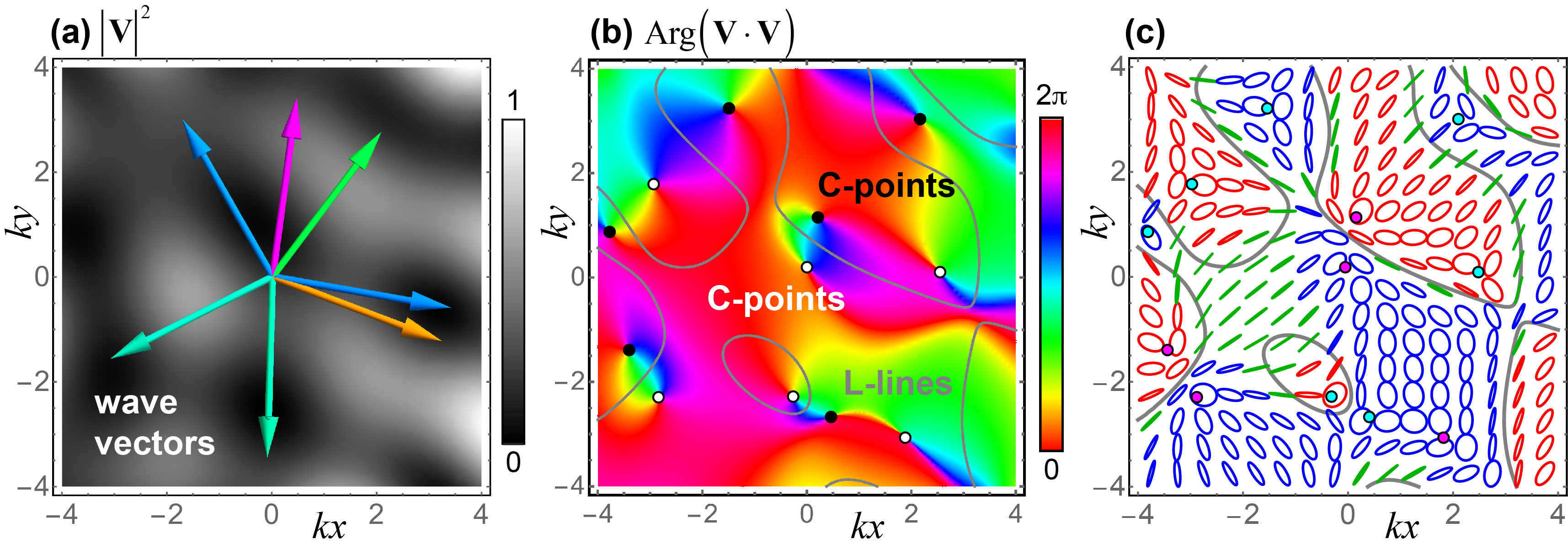
Figure 1: Random 2D acoustic field obtained by the interference of $N=7$ plane waves with the same frequency and amplitude but with random directions within the $(x,y)$ plane and random phases. (a) Wavevectors of the interfering waves (with color-coded phases) and distribution of the intensity of the velocity field $|{\bf V}|^{2}$ (greyscale). (b) Color-coded distribution of the phase of the quadratic field ${\bf V}\cdot{\bf V}$. The phase singularities (vortices) of this field correspond to C-points of purely circular polarization in the field ${\bf V}$. L-lines correspond to purely linear polarizations. (c) Distribution of the normalized polarization of ${\bf V}$. Red, blue, and green colors correspond to right-handed, left-handed, and near-linear polarizations, respectively. The C-points in a 2D polarization field can be labeled by two independent topological numbers Bliokh et al. (2019): (i) $n_{D}=1/2$ and $n_{D}=-1/2$ [black and white dots in (b), respectively] indicate half of the topological charge of the vortex in the quadratic field ${\bf V}\cdot{\bf V}$; (ii) $n_{C}=1/2$ and $n_{C}=-1/2$ [magenta and cyan dots in (c), respectively] correspond to the number of turns of the major semiaxis of the polarization ellipse along a closed contour including the C-point.

Being thoroughly described and observed for optical fields, polarization singularities and topological polarization structures have not been examined properly in sound and water waves. In this work, we fill this gap. We consider both random and regular structured acoustic and water-surface wavefields and show that polarization singularities and Möbius strips are also ubiquitous for them. These results can have a twofold impact. First, they provide a new platform for studying polarization singularities and topological structures. Importantly, while one cannot directly observe elliptical motion of the electric field ${\bm{\mathcal{E}}}$ or the vector-potential ${\bm{\mathcal{A}}}$ in optics, the velocity and displacement fields ${\bm{\mathcal{V}}}$ and ${\bm{\mathcal{R}}}$ are directly observable in acoustic and water-surface waves Taylor (1976); Gabrielson et al. (1995); www.saddleback.edu/faculty/jrepka/notes/waves.html ; Francois et al. (2017); Bliokh et al. (2020). Second, the vector representation of sound and water-surface waves can be relevant for wave-matter interactions, such as interactions with dipole particles coupled to the vector velocity field Toftul et al. (2019); Wei and Rodriguez-Fortuno (2020); Long et al. (2020b).

The paper is organized as follows. We start by presenting the generic appearance of C-points and L-lines in random 2D acoustic fields in Section II. Section III presents polarization singularities (C-points) in 3D acoustic fields, both random and regular, as well as polarization Möbius strips which appear around C-points. Section IV demonstrates the apperance of C-points and polarization Möbius strips in structured water-surface waves. Concluding remarks are provided in Section V.

II Polarization singularities in a 2D acoustic field

We consider monochromatic sound waves in a homogeneous fluid or gas, which are described by the equations Landau and Lifshitz (1987):

$$i\,\omega\,\beta\,P={\bm{\nabla}}\cdot{\bf{V}}\leavevmode\nobreak\ ,\quad i\,\omega\,\rho\,{\bf V}={\bm{\nabla}}P\leavevmode\nobreak\ .$$ (1)

Here, $\omega$ is the frequency, $\rho$ and $\beta$ are the density and compressibility of the medium, whereas $P({\bf r})$ and ${\bf V}({\bf r})$ are the complex pressure and velocity fields. The real time-dependent fields are ${{\mathcal{P}}}({\bf r},t)={\rm Re}[P({\bf r})\exp(-i\omega t)]$ and ${\bm{\mathcal{V}}}({\bf r},t)={\rm Re}[{\bf V}({\bf r})\exp(-i\omega t)]$.

The plane-wave solution of Eqs. (1) is

$$P=P_{0}\exp(i\,{\bf k}\cdot{\bf r})\leavevmode\nobreak\ ,\quad{\bf V}=V_{0}\,\bar{\bf k}\exp(i\,{\bf k}\cdot{\bf r})\leavevmode\nobreak\ ,$$ (2)

where $\bar{\bf k}={\bf k}/k$, ${\bf k}$ is the wavevector, $k=\omega/c$ is the wavenumber, $c=1/\sqrt{\rho\beta}$ is the speed of sound, and $P_{0}=\sqrt{\rho/\beta}\,V_{0}$. Sound waves are longitudinal because ${\bf V}\parallel{\bf k}$, but still have a vector nature described by the velocity field ${\bf V}$ Shi et al. (2019); Bliokh and Nori (2019b); Toftul et al. (2019); Rondón and Leykam (2019); Long et al. (2020a); Burns et al. (2020). In what follows, we will focus on the polarization properties of this vector wave field: the real velocity field ${\bm{\mathcal{V}}}({\bf r},t)$ at a given point ${\bf r}$ traces a polarization ellipse.

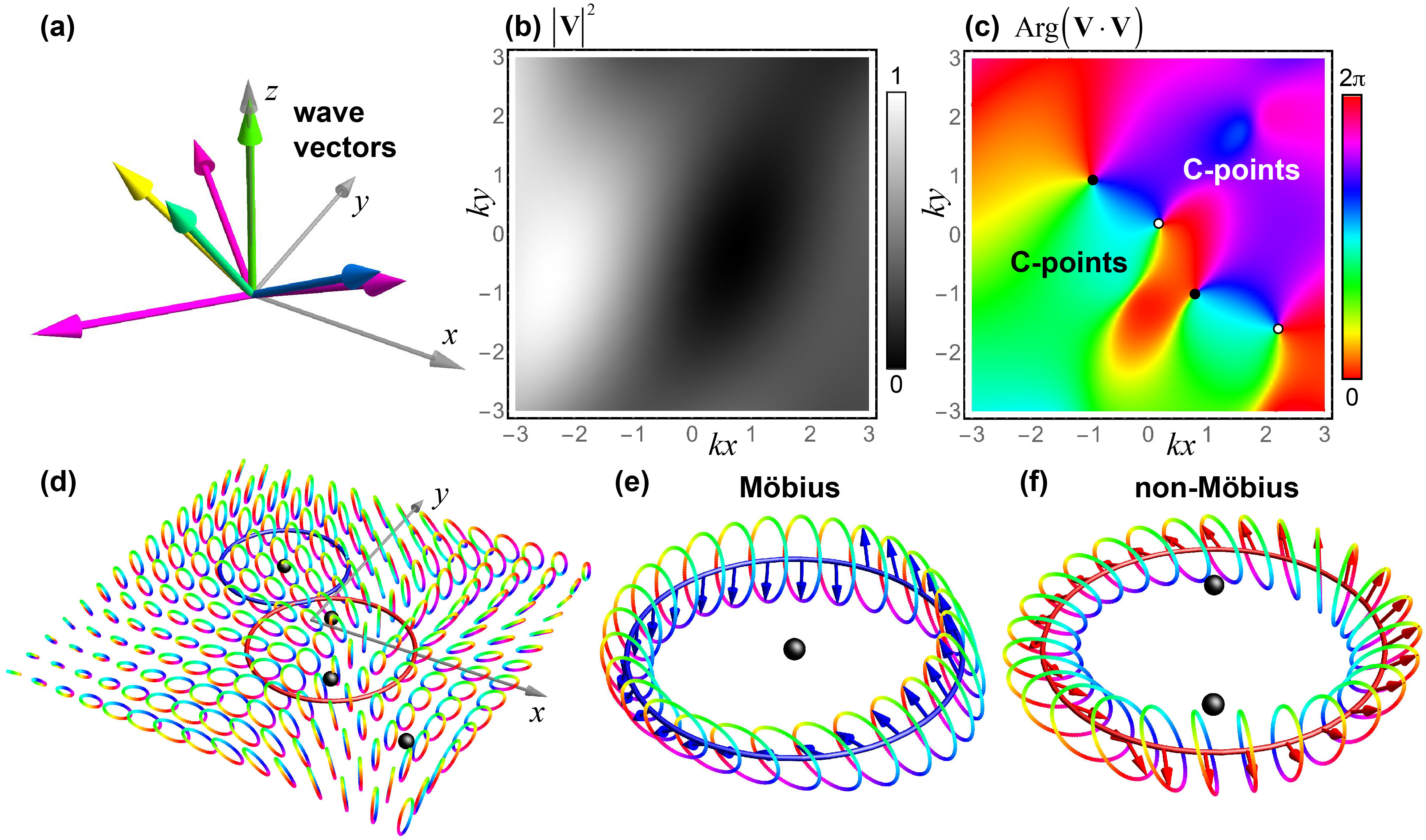
Figure 2: Random 3D acoustic field obtained by the interference of $N=7$ plane waves with the same frequency and amplitude but with random directions within the $k_{z}>0$ semisphere and random phases. (a) Wavevectors of the interfering waves with color-coded phases. (b) Distribution of the intensity of the velocity field $|{\bf V}|^{2}$ in the $z=0$ plane. (c) Color-coded distribution of the phase of the quadratic field ${\bf V}\cdot{\bf V}$ in the $z=0$ plane. Phase singularities (vortices) of this field correspond to C-points of purely circular polarization in the field ${\bf V}$. (d) Distribution of the normalized polarization ellipses of ${\bf V}$ in the $z=0$ plane. (e) Continuous evolution of polarization ellipses with their major semiaxes along a contour encircling a nondegenerate C-point exhibits a Möbius-strip structure Freund (2010a, b); Bauer et al. (2015). (f) For a contour encircling an even number of C-points (including zero), there is no polarization Möbius strip Bliokh et al. (2019).

We first examine a random speckle-like sound-wave field in 2D. Namely, we consider the interference of $N$ plane waves (2), ${\bf V}=\sum_{j=1}^{N}{\bf V}_{j}$, with wavevectors ${\bf k}_{j}$, $j=1,...,N$ randomly distributed over the circle $k_{x}^{2}+k_{y}^{2}=k^{2}$ ($k_{z}=0$), and with equal amplitudes $|V_{0j}|$ but random phases $\phi_{j}={\rm Arg}(V_{0j})$, as shown in Fig. 1(a). Due to the longitudinal character of sound waves, $V_{z}=0$, and the polarization ellipses of such field all lie in the $(x,y)$ plane. Figure 1 shows an example of such random field including its intensity and polarization distributions.

The distributions in Fig. 1 are similar to the corresponding distributions in random paraxial electromagnetic fields, with wavevectors directed almost along the $z$-axis and polarization ellipses approximately lying in the $(x,y)$ plane Nye (1983); Dennis et al. (2009); Bliokh et al. (2019). The only difference is that paraxial electromagnetic fields have a typical inhomogeneity scale of $(\theta k)^{-1}$, where $\theta\ll 1$ is the small characteristic angle between the wavevectors and the $z$-axis, while in the acoustic case $\theta=\pi/2$ and the typical inhomogeneity scale is $k^{-1}$. Polarization singularities of generic 2D polarization fields are the C-points of purely-circular polarization and L-lines of purely-linear polarization Nye and Hajnal (1987); Berry and Dennis (2001); Nye (1983); Hajnal (1987); Dennis et al. (2009); Bliokh et al. (2019), as shown in Figs. 1(b,c).

C-points correspond to phase sigularities (vortices) in the scalar field $\Psi({\bf r})={\bf V}({\bf r})\cdot{\bf V}({\bf r})$ Berry and Dennis (2001); Dennis et al. (2009); Bliokh et al. (2019), Fig. 1(b). Notably, these points generically coincide neither with zeros of the scalar pressure field $P({\bf r})$, nor with zeros of $|{\bf V}({\bf r})|^{2}$. Furthermore, each C-point in a 2D polarization field can be characterized by two half-integer topological numbers Bliokh et al. (2019). The first, $n_{C}$, corresponds to the number of turns of the major semiaxis of the polarization ellipse along a closed contour including the C-point. The second, $n_{D}$, is half the topological charge of the corresponding phase singularity in the field $\Psi$. In the generic (non-degenerate) case, singularities have the topological numbers $n_{C}=\pm 1/2$ and $n_{D}=\pm 1/2$ (see Fig. 1). Note that the morphological classification of 2D polarization distributions around C-points, such as ‘stars’, ‘lemons’, and ‘monstars’, is thoroughly described for optical polarized fields Dennis (2002); Dennis et al. (2009) and applies here as well. Note also that higher-order singularities can appear in degenerate cases, e.g., with imposed additional symmetries, such as cylindrical beams.

III C-points and polarization Möbius strips in 3D acoustic fields

III.1 Random fields

Akin to nonparaxial 3D electromagnetic fields, generic sound-wave fields have polarization characterized by the ellipses traced by the velocity field ${\bm{\mathcal{V}}}({\bf r},t)$ at every point ${\bf r}$, which can be arbitrarily oriented in 3D space. To show an example of such field, we consider an interference of $N$ plane waves with equal amplitudes $|V_{0j}|$, wavevectors ${\bf k}_{j}$, $j=1,...,N$, with directions randomly distributed over the hemisphere $k_{z}>0$ ($k_{x}^{2}+k_{y}^{2}+k_{z}^{2}=k^{2}$), and random phases $\phi_{j}={\rm Arg}(V_{0j})$, see Fig. 2(a).

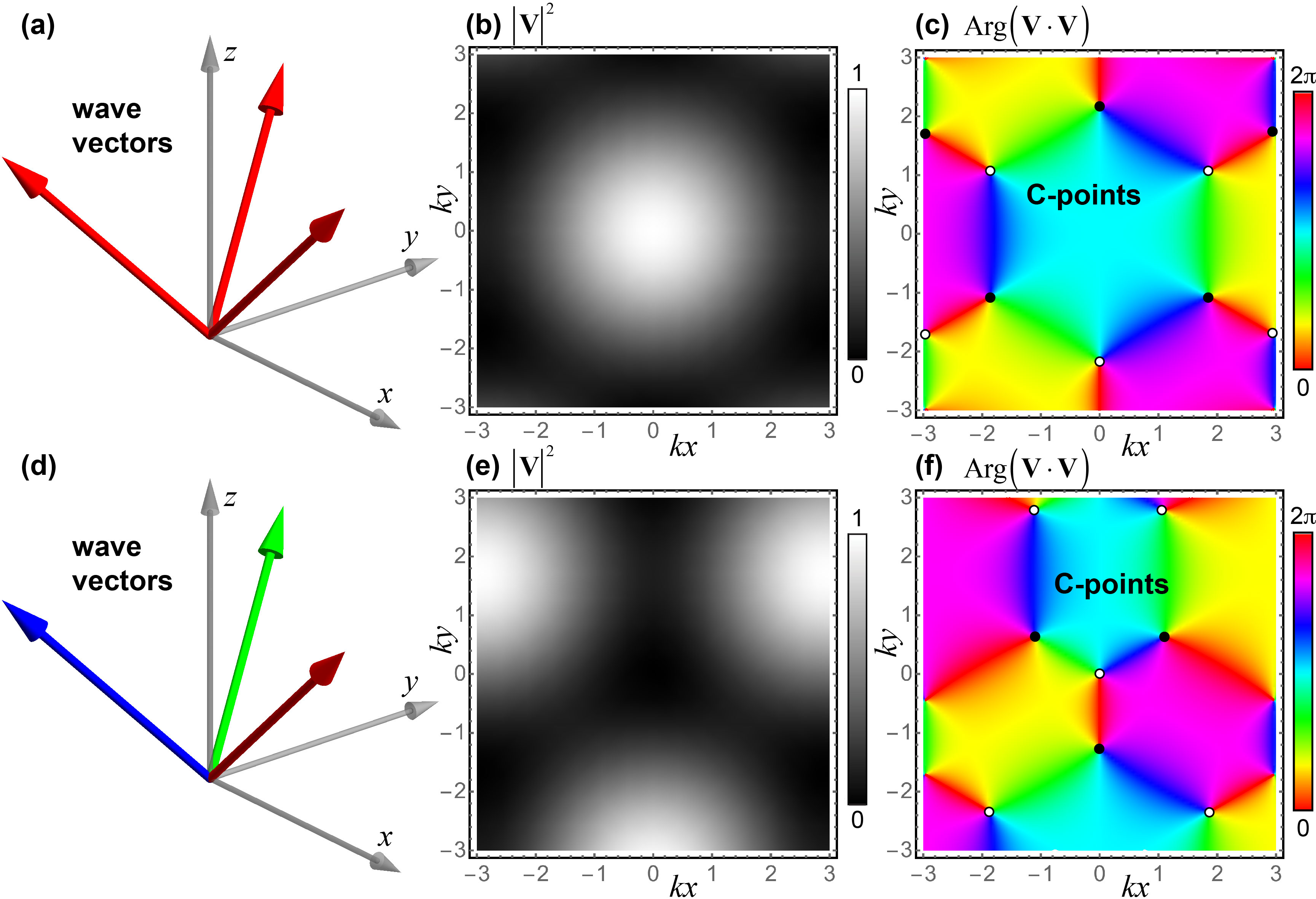
Figure 3: The wavevectors ${\bf k}_{j}$, distributions of the intensity of the velocity field, $|{\bf V}|^{2}$, and of the phase of the quadratic field ${\bf V}\cdot{\bf V}$ in the $z=0$ plane, for the three-wave superpositions (3) with $N=3$, $\theta_{0}=\pi/4$, $\ell=0$ (a,b,c) and $\ell=1$ (d,e,f).

The distributions of the resulting intensity $|{\bf V}|^{2}$ and of the phase of the quadratic field ${\bf V}\cdot{\bf V}$ over the $z=0$ plane are shown in Figs. 2(b,c). Similar to the 2D case, the phase singularities of the quadratic field correspond to the C-points (polarization singularities) in the polarization distribution, Fig. 2(d). However, in the 3D case, the circular polarizations in these points do not generically lie in the $(x,y)$ plane Nye and Hajnal (1987); Berry and Dennis (2001); Dennis et al. (2009); Bliokh et al. (2019).

Furthermore, distributions of the 3D polarization ellipses in the vicinity of C-points have remarkable topological properties. Namely, continuous evolution of the major semiaxes of the polarization ellipse along a contour encircling a non-degenerate C-point traces a 3D Möbius-strip-like structure Freund (2010a, b); Bauer et al. (2015); Galvez et al. (2017); Garcia-Etxarri (2017); Kreismann and Hentschel (2018); Bauer et al. (2019); Tekce et al. (2019); Bliokh et al. (2019), Fig. 2(e). Notably, the number of turns of the polarization ellipse around the contour is not topologically stable: continuous deformations of the contour (without crossing C-points) can result in the change of the number of turns by an integer number Dennis (2011); Freund (2020a). However, the number of turns modulo 1/2, which distinguish the ‘Möbius’ (half-integer number of turns) and ‘non-Möbius’ (integer number of turns) cases is topologically stable. It directly corresponds to the number of C-points enclosed by the contour modulo 2 Bliokh et al. (2019), see Figs. 2(d,e,f).

Recently, polarization Möbius strips attracted great attention in optics Bauer et al. (2015); Galvez et al. (2017); Garcia-Etxarri (2017); Kreismann and Hentschel (2018); Bauer et al. (2019); Tekce et al. (2019); Bliokh et al. (2019). We argue that entirely similar polarization structures naturally appear in inhomogeneous sound-wave fields. In addition to the random field shown in Fig. 2, below we consider examples of regular sound-wave fields with polarization singularities and Möbius strip.

III.2 Three-wave interference

We now consider examples of regular (non-random) 3D acoustic fields with polarization singularities and Möbius strips. In optics, such singularities are often generated in vector vortex beams Dennis et al. (2009); Bauer et al. (2015); Galvez et al. (2017); Bauer et al. (2019); Tekce et al. (2019); Bliokh et al. (2019). Here we also consider a superposition of $N$ acoustic plane waves with wavevectors evenly distributed within a cone of polar angle $\theta=\theta_{0}$ and with an azimuthal phase difference corresponding to a vortex of order $\ell$:

$${\bf V}=V_{0}\,\sum_{j=1}^{N}\bar{\bf k}_{j}\exp\!\left[i\,{\bf k}_{j}\cdot{\bf r}+i\,\ell\,\phi_{j}\right]\leavevmode\nobreak\ ,$$ (3)

where ${\bf k}_{j}=k\left(\sin\theta_{0}\cos\phi_{j},\,\sin\theta_{0}\sin\phi_{j},\,\cos\theta_{0}\right)$ and $\phi_{j}=2\pi(j-1)/N$. In the limit of $N\gg 1$, this superposition tends to an acoustic Bessel beam Bliokh and Nori (2019b).

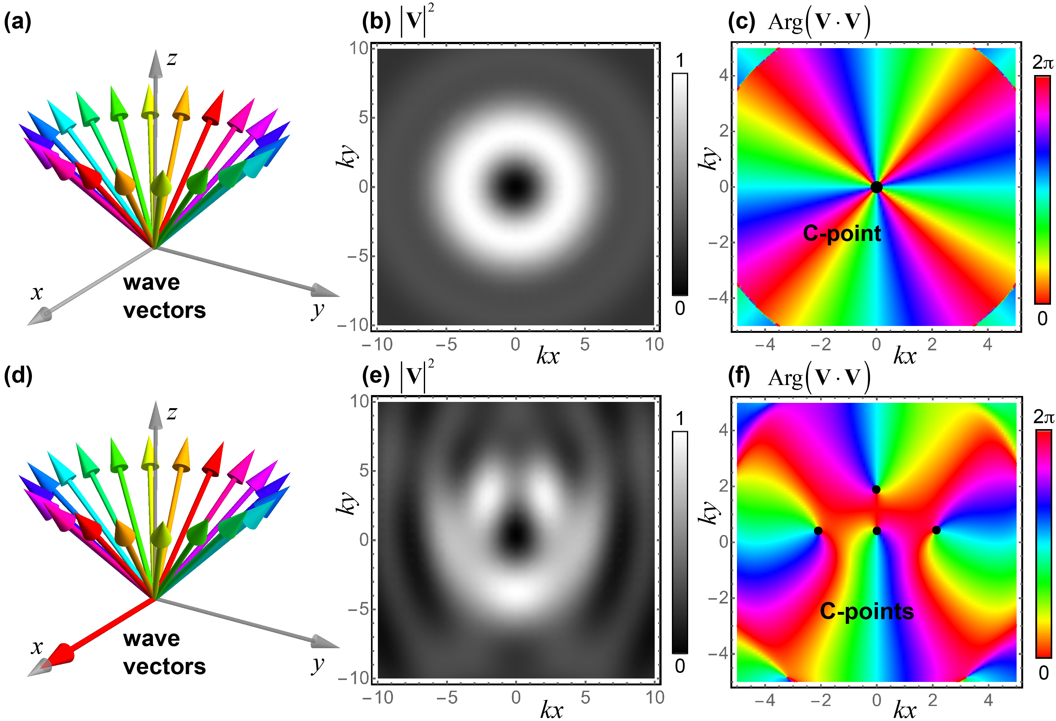
Figure 4: The wavevectors, distributions of the intensity of the velocity field, $|{\bf V}|^{2}$, and of the phase of the quadratic field ${\bf V}\cdot{\bf V}$ in the $z=0$ plane, for the Bessel-beam superposition (3) with $N=20$, $\theta_{0}=\pi/4$, $\ell=2$ (a,b,c) and the same Bessel beam interfering with an additional plane wave, Eq. (4), with $V^{\prime}/V_{0}=2$ (d,e,f). One can see the splitting of the even-order C-point (integer $n_{D}=\ell$) (c) into $2|n_{D}|$ first-order C-points (f) when breaking the cylindrical symmetry of the vortex beam.

The minimal number of plane waves to generate polarization singularities is $N=3$. Figure 3 shows the wavevectors ${\bf k}_{j}$, distributions of the intensity of the velocity field, $|{\bf V}|^{2}$, and of the phase of the quadratic field, ${\rm Arg}({\bf V}\cdot{\bf V})$, for the three-wave superpositions (3) with $\theta_{0}=\pi/4$, $\ell=0$ and $\ell=1$. One can see a number of first-order C-points, i.e., phase singularities in the quadratic field ${\bf V}\cdot{\bf V}$. Accordingly, 3D polarization ellipses along a contour enclosing an odd number of C-points form polarization Möbius strips. Importantly, the spacing between the C-points in Fig. 3 is controlled by the polar angle $\theta_{0}$. When $\theta_{0}\ll 1$ (paraxial regime), the C-points merge and form only even-order C-points with no Möbius strips around them. In particular, the four C-points at the center of Fig. 3(f) with the integer total topological charge $n_{D}=3/2-1/2=1$ merge into a single second-order ($n_{D}=1$) C-point in the paraxial limit. This is in sharp contrast to the electromagnetic (optical) waves, where isolated first-order C-points can appear even in the paraxial case.

III.3 Perturbed vortex beams

Consider now the large-$N$ limit of the superposition (3), which generates acoustic vortex (Bessel) beams. Due to the cylindrical symmetry, such beams can have an isolated C-point at the center. However, in contrast to optical vectorial vortex beams, the C-point at the center of an acoustic vortex beam always has an even order (integer $n_{D}=\ell$) Bliokh and Nori (2019b) (see Fig. 4). This does not allow one to generate an acoustic polarization Möbius strip in a symmetric vortex configuration as in optics Bauer et al. (2015); Galvez et al. (2017); Bauer et al. (2019); Tekce et al. (2019); Bliokh et al. (2019). However, breaking the cylindrical symmetry of the beam results in splitting of the even-order C-point at the center into a number of the first-order C-points ($n_{D}=\pm 1/2$), each of which carries polarization Möbius strip structures around it. For example, one can break the symmetry by interfering the vortex beam with a horizontally-propagating plane wave:

$${\bf V}={\bf V}_{\rm vortex}+V^{\prime}\bar{\bf k}^{\prime}\exp(i\,{\bf k}^{\prime}\cdot{\bf r})\leavevmode\nobreak\ ,$$ (4)

where ${\bf V}_{\rm vortex}$ is the vortex-beam field, such as Eq. (3) with $N\gg 1$, whereas ${\bf k}^{\prime}=k(1,0,0)$. Figure 4 shows the splitting of the even-order C-point at the center of an acoustic vortex beam into first-order C-points when interfering the beam with a horizontally-propagating plane wave.

The above examples show that the typical spacing between the C-points in structured sound waves is $k^{-1}$, and this spacing can decrease in the paraxial regime and in the presence of additional symmetries. This also determines the typical subwavelength size of the acoustic polarization Möbius strips.

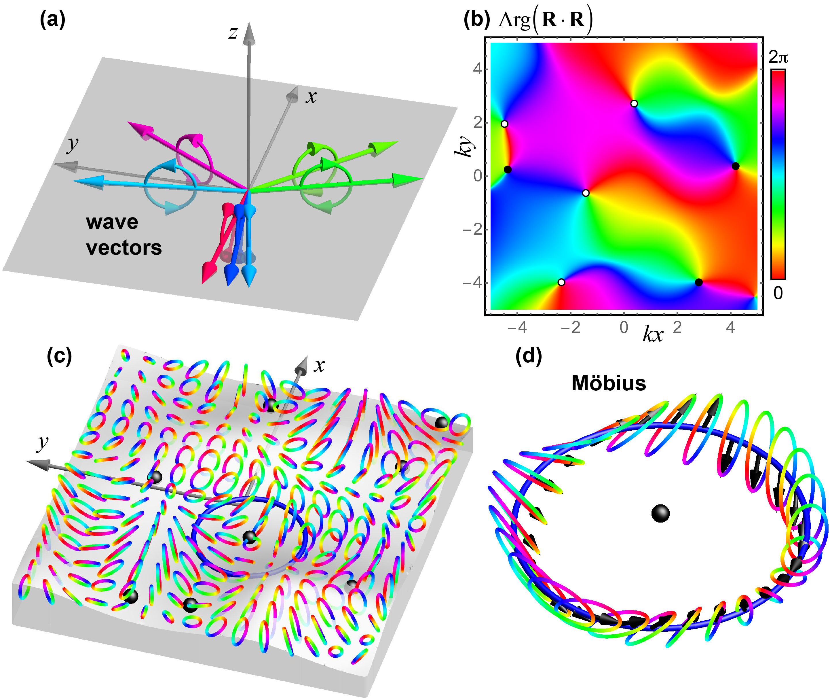
Figure 5: Random 3D water-surface wave field obtained by the interference of $N=7$ plane waves with the same frequency and amplitude but with random directions in the $(x,y)$ plane and random phases. (a) Wavevectors of the interfering waves with color-coded phases and their circular polarizations. (b) Color-coded distribution of the phase of the quadratic field ${\bf R}\cdot{\bf R}$ in the water-surface $z=0$ plane. Phase singularities (vortices) of this field correspond to C-points of purely circular polarization in the field ${\bf R}$. (c) Distribution of the normalized polarization ellipses of the ${\bf R}$ field in the $z=0$ plane. These ellipses are trajectories of water-surface particles (Multimedia view). The instantaneous water surface at $t=0$ is shown in gray. (d) Akin to Fig. 2, the continuous evolution of polarization ellipses with their major semiaxes along a contour encircling a C-point exhibits a polarization Möbius strip (Multimedia view).

IV Polarization singularities and Möbius strips in water-surface waves

One of the key differences between electromagnetic and acoustic fields is that the electric and magnetic fields are vectors in abstract spaces of the field components (there is no ‘ether’ and nothing moves in a free-space electromagnetic wave), while the velocity field corresponds to the motion of the medium’s particles (atoms or molecules) in real space. Moreover, instead of the velocity field, one can consider the displacement field ${\bm{\mathcal{R}}}({\bf r},t)$: ${\bm{\mathcal{V}}}=\partial_{t}{\bm{\mathcal{R}}}$, or, for a monochromatic field in the complex representation, ${\bf V}=-i\,\omega\,{\bf R}$. The displacement field can be regarded as a ‘vector-potential’ for the velocity field Burns et al. (2020). It has the same polarization, but the polarization ellipses traced by ${\bm{\mathcal{R}}}$ correspond to real-space trajectories of the medium particles.

This opens an avenue to the direct observation of polarization ellipses and more complicated structures Sugic et al. (2020). In sound waves, typical displacement amplitudes are small and their direct observations are challenging Taylor (1976); Gabrielson et al. (1995). However, similar medium displacements can be easily observed in another type of classical waves, namely, water-surface (e.g., gravity or capillary) waves Landau and Lifshitz (1987), with typical displacement scales ranging from milimeters to meters. Recently, there were several studies on polarization properties of structured water waves Francois et al. (2017); Bliokh et al. (2020); Sugic et al. (2020), and here we show that these waves naturally reveal generic polarization singularities.

For the sake of simplicity, we consider deep-water gravity waves on the unperturbed water surface $z=0$ Landau and Lifshitz (1987). The equations of motion for the complex displacement field ${\bf R}=(X,Y,Z)$ of the water-surface particles in a monochromatic wave field can be written in a form similar to the acoustic equations (1) Bliokh et al. (2020); Sugic et al. (2020):

$$\omega^{2}Z=-g\,{\bm{\nabla}}_{\perp}\cdot{\bf R}_{\perp}\leavevmode\nobreak\ ,\quad\omega^{2}{\bf R}_{\perp}=g\,{\bm{\nabla}}_{\perp}Z\leavevmode\nobreak\ .$$ (5)

Here $g$ is the gravitational acceleration, ${\bf R}_{\perp}=(X,Y)$, and ${\bm{\nabla}}_{\perp}=(\partial_{x},\partial_{y})$. Making the plane-wave ansatz ${\bm{\nabla}}_{\perp}\to i\,{\bf k}$, ${\bf k}=(k_{x},k_{y})$, in Eqs. (5), we obtain the dispersion relation $\omega^{2}=gk$.

The plane-wave solution of Eqs. (5) is:

$$Z=Z_{0}\exp(i\,{\bf k}\cdot{\bf r})\leavevmode\nobreak\ ,\quad{\bf R}_{\perp}=i\,Z_{0}\,\bar{\bf k}\exp(i\,{\bf k}\cdot{\bf r})\leavevmode\nobreak\ .$$ (6)

These relations show that deep-water gravity waves have equal longitudinal (${\bf k}$-directed) and transverse ($z$-directed) displacement components phase-shifted by $\pi/2$ with respect to each other. In other words, such plane waves are circularly polarized in the meridional (propagation) plane including the wavevector and the normal to the unperturbed water surface www.saddleback.edu/faculty/jrepka/notes/waves.html . Such (generically, elliptical) meridional polarization is a common feature of surface and evanescent waves in different physical contexts Shi et al. (2019); Bliokh and Nori (2019a, 2015); Aiello et al. (2015). Therefore, interfering plane water waves with wavevectors lying in the $(x,y)$ plane results in generic 3D polarization structures with all three components of the displacement field ${\bf R}$.

To show that such polarization distributions generically posses polarization singularities, we consider the interference of $N$ plane waves (6): ${\bf R}=\sum_{j=1}^{N}{\bf R}_{j}\equiv\sum_{j=1}^{N}{\bf R}_{0j}\exp(i\,{\bf k}_{j}\cdot{\bf r}_{\perp})$, with ${\bf R}_{0j}=Z_{0j}(i\bar{k}_{jx},i\bar{k}_{jy},1)$, wavevectors ${\bf k}_{j}$ randomly distributed over the circle $k_{x}^{2}+k_{y}^{2}=k^{2}$, and equal amplitudes $|Z_{0j}|$ but random phases $\phi_{j}={\rm Arg}(Z_{0j})$, as shown in Fig. 5(a) (cf. Fig. 1). Figure 5(b) shows the phase distribution of the quadratic field $\Psi={\bf R}\cdot{\bf R}$; it clearly exhibits phase singularities corresponding to C-points of the vector field ${\bf R}$. The distribution of the polarization ellipses, i.e., trajectories of the water-surface particles, over the $z=0$ plane is shown in Fig. 5(c) (Multimedia view). Tracing the orientation of the polarization ellipses along a contour encircling a C-point reveals the generic Möbius-strip structure, Fig. 5(d) (Multimedia view). We also provide animated versions of Figs. 5(c,d), where one can see motion of the water surface and separate water particles. In particular, the animated version of Fig. 5(d) shows the temporal evolution of the displacement vectors $\bm{\mathcal{R}}({\bf r},t)$ along the contour, which can form ‘twisted ribbon carousels’ Freund (2020b).

Thus, by tracing 3D trajectories of water particles in a random (yet monochromatic) water-surface wavefield one can directly observe generic polarization singularities of 3D vector wavefields.

V Concluding remarks

This work was motivated by recent strong interest in (i) polarization Möbius strips in 3D polarized optical fields Freund (2010a, b); Dennis (2011); Bauer et al. (2015); Galvez et al. (2017); Garcia-Etxarri (2017); Kreismann and Hentschel (2018); Bauer et al. (2019); Tekce et al. (2019); Bliokh et al. (2019) and (ii) vectorial spin properties of acoustic and water-surface waves Shi et al. (2019); Bliokh and Nori (2019a, b); Toftul et al. (2019); Rondón and Leykam (2019); Long et al. (2020a); Burns et al. (2020); Bliokh et al. (2020); Sugic et al. (2020). We have shown that these research directions can be naturally coupled, and that polarization singularities, such as C-points and polarization Möbius strips, are ubiquitous for inhomogeneous (yet monochromatic) acoustic and water-surface waves. The vector velocity or displacement of the medium particles provide complex-valued elliptical polarization fields varying across the space. We have considered various examples of random and regular interference fields consisting of multiple (three or more) plane waves, which exhibit polarization singularities and Möbius strips.

In contrast to well-studied electromagnetic polarizations associated with the motion of abstract field vectors, acoustic and water-wave polarizations correspond to real-space trajectories of the medium particles. In particular, these are readily directly observable for water-surface waves Francois et al. (2017); Bliokh et al. (2020). Also, while optical vectorial-vortex beams can bear an isolated first-order C-point and a Möbius strip around it Bauer et al. (2015); Galvez et al. (2017); Bauer et al. (2019); Tekce et al. (2019); Bliokh et al. (2019), acoustic C-points typically appear in clusters with subwavelength distance between the points.

Analyzing wave-field singularities is useful because of their topological robustness; they provide a ‘skeleton’ of an inhomogeneous field Nye (1999). This robustness is highly important because real-life waves in fluids always have inherent perturbations, such as viscosity and nonlinearity, with respect to the idealized non-dissipative linear picture. So far, only phase singularities of the scalar pressure field $P$ were considered in sound-wave fields. The vector velocity field ${\bf V}\propto\bm{\nabla}P$ and its polarization singularities provide an alternative representation and can be more relevant, e.g., in problems involving dipole wave-matter coupling. Note that the vectorial representation of a gradient of a scalar wavefield was previously considered in Ref. Dennis (2004).

For water-surface waves, the scalar representation is based on the vertical displacement field $Z$. Tidal ocean waves were also studied in terms of the 2D polarization field of the horizontal current Hansen (1952); Berry (2001); Nye et al. (1988); Ray (2001); Ray and Egbert (2004) associated with the velocity components $(V_{x},V_{y})$. We argue that these scalar and 2D vector fields can be regarded as components of a single 3D vector displacement ${\bf R}$ or velocity ${\bf V}$ field. Moreover, we have considered gravity deep-water waves, which are much more feasible for experimental laboratory studies than tidal waves Francois et al. (2017); Bliokh et al. (2020).

Notably, our arguments are not restricted to purely sound and water-surface waves. They can be equally applied to any fluid/gas or fluid/fluid surface waves as well as internal gravity waves in stratified fluid or gas media. We hope that our work will stimulate further studies and possibly applications of 3D polarization textures and topological vectorial properties of various waves in acoustics and fluid mechanics.