Machine-Learned Phase Diagrams of Generalized Kitaev Honeycomb Magnets

Abstract

We use a recently developed interpretable and unsupervised machine-learning method, the tensorial kernel support vector machine (TK-SVM), to investigate the low-temperature classical phase diagram of a generalized Heisenberg-Kitaev-$\Gamma$ ($J$-$K$-$\Gamma$) model on a honeycomb lattice. Aside from reproducing phases reported by previous quantum and classical studies, our machine finds a hitherto missed nested zigzag-stripy order and establishes the robustness of a recently identified modulated $S_{3}\times Z_{3}$ phase, which emerges through the competition between the Kitaev and $\Gamma$ spin liquids, against Heisenberg interactions. The results imply that, in the restricted parameter space spanned by the three primary exchange interactions—$J$, $K$, and $\Gamma$, the representative Kitaev material $\alpha$-${\rm RuCl}_{3}$ lies close to the boundaries of several phases, including a simple ferromagnet, the unconventional $S_{3}\times Z_{3}$ and nested zigzag-stripy magnets. A zigzag order is stabilized by a finite $\Gamma^{\prime}$ and/or $J_{3}$ term, whereas the four magnetic orders may compete in particular if $\Gamma^{\prime}$ is anti-ferromagnetic.

I Introduction

Machine learning (ML) is quickly developing into a powerful tool in modern day physics research Carleo et al. (2019); Mehta et al. (2019). Successful applications in condensed-matter physics can be found in, for example, detecting phases and phase transitions Wang (2016); Ponte and Melko (2017); Carrasquilla and Melko (2017); Chen et al. (2020), representing and solving quantum wave functions Carleo and Troyer (2017); Carrasquilla (2020); Deng et al. (2017); Hermann et al. (2020); Pfau et al. (2020); Vieijra et al. (2020), analyzing experiments Nussinov et al. (2016); Zhang et al. (2019); Bohrdt et al. (2019), searching new materials Schmidt et al. (2019), and designing algorithms Liao et al. (2019); Liu et al. (2017). Recent developments of ML in strongly correlated condensed matter physics are moving beyond benchmarking, and the ultimate goal is to provide toolboxes to tackle hard and open problems.

The Kitaev materials Takagi et al. (2019); Janssen and Vojta (2019); Winter et al. (2017a) are prime candidates for a challenging application of ML, hosting various disordered and unconventionally ordered phases. Experimentally, the bond-dependent anisotropic interactions of the Kitaev honeycomb model Kitaev (2006) are realized through electron correlations and spin-orbit coupling Jackeli and Khaliullin (2009); Chaloupka et al. (2010). Representative compounds include $4d$ and $5d$ transition-metal-based Mott insulators ${\rm A}_{2}{\rm IrO}_{3}$ ($\text{A}=\text{Na, Li, K}$) and $\alpha$-${\rm RuCl}_{3}$ Winter et al. (2017a); Banerjee et al. (2016, 2017); Ran et al. (2017); Yadav et al. (2016, 2019); Chaloupka and Khaliullin (2015). In particular, the latter material has been proposed to host a field-induced quantum spin liquid as evidenced by the half-quantized thermal Hall effect under external magnetic field Kasahara et al. (2018); Yokoi et al. (2020), while spectroscopic Ponomaryov et al. (2020); Sahasrabudhe et al. (2020); Maksimov and Chernyshev (2020) and thermodynamic Bachus et al. (2020, 2021) measurements indicate a topologically trivial partially-polarized phase. More recently, the cobaltate systems ${\rm Na}_{3}{\rm Co}_{2}{\rm SbO}_{6}$ and ${\rm Na}_{2}{\rm Co}_{2}{\rm TeO}_{6}$ Viciu, L. and Huang, Q. and Morosan, E. and Zandbergen, H. W. and Greenbaum, N. I. and McQueen, T. and Cava, R. J. (2007); Liu and Khaliullin (2018); Liu et al. (2020); Songvilay et al. (2020) and Cr-based pseudospin-$3/2$ systems ${\rm CrSiTe}_{3}$ and ${\rm CrGeTe}_{3}$ Xu et al. (2020) were added to this family.

In the ideal case, one expects to find a compound that faithfully exhibits the physics of the Kitaev model. However, non-Kitaev terms, such as the Heisenberg exchange and the symmetric off-diagonal $\Gamma$ exchange, are permitted by the underlying cubic symmetry and ubiquitously exist in real Kitaev materials Rau et al. (2014, 2016). In addition, longer-range interactions and structural distortions can lead to further hopping channels Rau and Kee (2014); Rusnačko et al. (2019); Maksimov and Chernyshev (2020). These additional terms enrich the Kitaev physics Wang et al. (2019); Gohlke et al. (2018, 2020); Chern et al. (2020); Lee et al. (2020); Jiang et al. (2019); Gordon et al. (2019); Rusnačko et al. (2019); Lampen-Kelley et al. (2018); Liu et al. (2021) but also pose a significant challenge to the analysis because of the large parameter space and the emergence of complicated structures. Therefore, tools that can efficiently detect patterns and important information in data and construct the associated phase diagrams are called for.

In this work, we use our recently developed tensorial-kernel support vector machine (TK-SVM) Greitemann et al. (2019a); Liu et al. (2019); Greitemann et al. (2019b) to investigate the phase diagram of a generalized Heisenberg-Kitaev-$\Gamma$ model on a honeycomb lattice. This method is interpretable and unsupervised, equipped with a tensorial kernel and graph partitioning. The tensorial kernel detects both linear and high-order correlations, and the results can systematically be interpreted as meaningful physical quantities, such as order parameters Greitemann et al. (2019a) and emergent local constraints Greitemann et al. (2019b). Moreover, in virtue of the graph partitioning module, phase diagrams can be constructed without supervision and prior knowledge.

In our previous investigation of the Kitaev magnets we applied TK-SVM to the classical $K$-$\Gamma$ model subject to a magnetic field Liu et al. (2021). There, our machine learned a rich global phase diagram, revealing, among others, two novel modulated $S_{3}\times Z_{3}$ phases, which originate from the competition between the Kitaev and $\Gamma$ spin liquids. This work explores the low-temperature classical phase diagram of the generic Heisenberg-Kitaev-$\Gamma$ ($J$-$K$-$\Gamma$) model as well as the effect of the $\Gamma^{\prime}$ and third nearest-neighbor Heisenberg ($J_{3}$) terms, which are sub-leading exchange terms commonly encountered in the class of Kitaev materials. From our findings it follows that in the parameter space spanned by $J$,$K$, and $\Gamma$, the representative Kitaev material $\alpha$-${\rm RuCl}_{3}$ lies close to several competing phases, including a hitherto missed nested zigzag-stripy magnet, a previously identified $S_{3}\times Z_{3}$ magnet, a ferromagnet, and a possibly correlated paramagnet (Section III). Zigzag order can be stabilized by including a small $\Gamma^{\prime}$ and/or anti-ferromagnetic $J_{3}$ term. However, if the $\Gamma^{\prime}$ is also antiferromagnetic, this material resides in a region where these four magnetic orders strongly compete (Section IV). Our results constitute therefore one of the earliest examples of ML going beyond the state of the art in strongly correlated condensed matter physics.

This paper is organized as follows. In Section II, we define the generalized Heisenberg-Kitaev-$\Gamma$ model and specify the interested parameter regions. The machine-learned $J$-$K$-$\Gamma$ phase diagrams in the absence and presence of additional $J_{3}$ and $\Gamma^{\prime}$ terms are discussed and validated in Section III and Section IV, respectively. Section V discusses the implications of our results for representative Kitaev compounds. In Section VI we conclude and provide an outlook. In addition, a brief summary of TK-SVM and details about the training procedure and Monte Carlo simulations are provided in Appendices.

II Honeycomb $J$-$K$-$\Gamma$-$\Gamma^{\prime}$-$J_{3}$ Model

We study the generalized Heisenberg-Kitaev-$\Gamma$ model on a honeycomb lattice

$$H =H_{JK\Gamma}+H_{\Gamma^{\prime}}+H_{J_{3}},$$

$$=\sum_{\langle ij\rangle_{\gamma}}\mathbf{S}_{i}\cdot\hat{\mathcal{J}}_{\gamma}\mathbf{S}_{j}+\sum_{(ij)}J_{3}\mathbf{S}_{i}\cdot\mathbf{S}_{j},$$ (1)

where

$$H_{\scalebox{0.618}{$JK\Gamma$}}\!=\!\sum_{\langle ij\rangle_{\gamma}}\big{[}J\mathbf{S}_{i}\cdot\mathbf{S}_{j}\!+\!KS_{i}^{\gamma}S_{j}^{\gamma}\!+\!\Gamma(S_{i}^{\alpha}S_{j}^{\beta}+S_{i}^{\beta}S_{j}^{\alpha})\big{]},$$ (2)

$$H_{\Gamma^{\prime}}=\sum_{\langle ij\rangle_{\gamma}}\big{[}\Gamma^{\prime}(S_{i}^{\gamma}S_{j}^{\alpha}+S_{i}^{\gamma}S_{j}^{\beta}+S_{i}^{\alpha}S_{j}^{\gamma}+S_{i}^{\beta}S_{j}^{\gamma})\big{]}.$$ (3)

Here, $\gamma$ labels the three distinct nearest-neighbor (NN) bonds $\langle ij\rangle$ with mutually exclusive $\alpha,\beta,\gamma\in\{x,y,z\}$ as illustrated in Figure 1; $\hat{\mathcal{J}}_{\gamma}$ is a $3\times 3$ matrix comprising all exchanges on a NN bond $\langle ij\rangle_{\gamma}$, and $(ij)$ denotes the third NN bonds with a Heisenberg interaction $J_{3}$.

The Heisenberg-Kitaev-$\Gamma$ Hamiltonian Eq. (2) comprises generic NN exchanges allowed by the cubic symmetry Jackeli and Khaliullin (2009); Rau et al. (2014). Although the Kitaev ($K$) term is of prime interest for realizing quantum Kitaev spin liquids, the Heisenberg ($J$) and the symmetric off-diagonal ($\Gamma$) exchanges ubiquitously exist and play a key role in the physics of realistic materials. The $\Gamma^{\prime}$ term is a secondary symmetric off-diagonal interaction and originates from a trigonal distortion of the octahedral environment of magnetic ions. A negative (positive) $\Gamma^{\prime}$ corresponds to trigonal compression (expansion) of the edge-sharing oxygen or chlorine octahedra Rau and Kee (2014) while the inclusion of the $J_{3}$ term reflects the extension of $d$-electron wave functions. Although second nearest-neighbor exchanges are also possible, the third-neighbor exchanges are found to be more significant in representative Kitaev magnets, including the intensely studied compounds ${\rm Na}_{2}{\rm IrO}_{3}$, $\alpha$-${\rm Li}_{2}{\rm IrO}_{3}$, $\alpha$-${\rm RuCl}_{3}$ and the more recently (re-)characterized cobalt-based compounds ${\rm Na}_{3}{\rm Co}_{2}{\rm SbO}_{6}$ and ${\rm Na}_{2}{\rm Co}_{2}{\rm TeO}_{6}$ Viciu, L. and Huang, Q. and Morosan, E. and Zandbergen, H. W. and Greenbaum, N. I. and McQueen, T. and Cava, R. J. (2007); Songvilay et al. (2020). Aside from the potential microscopic origin, the $\Gamma^{\prime}$ and $J_{3}$ exchange terms are often introduced phenomenologically to stabilize magnetic orders observed in experiments Banerjee et al. (2017); Rusnačko et al. (2019); Laurell and Okamoto (2020); Maksimov and Chernyshev (2020), in particular the zigzag-type orders found in many two-dimensional Kitaev materials Takagi et al. (2019).

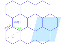
Figure 1: A honeycomb lattice with anisotropic bonds $\gamma(\alpha\beta)$. The shaded region marks a symmetric cluster of $m\times m$ unit cells. A lattice with linear size $L$ is then partitioned into $(\frac{L}{m})^{2}$ such clusters. Here, $m=2$ is shown for example. Larger clusters with $m=4,6,12$ are considered in training TK-SVMs.

It is commonly expected that the primary physics in a Kitaev material is governed by the interactions in the $H_{JK\Gamma}$ model, whose phase diagram for fixed $\Gamma^{\prime}$ and $J_{3}$ is the topic of the present work. Moreover, motivated by the microscopic models proposed for $\alpha$-${\rm RuCl}_{3}$ Maksimov and Chernyshev (2020); Laurell and Okamoto (2020), ${\rm Na}_{3}{\rm Co}_{2}{\rm SbO}_{6}$ and ${\rm Na}_{2}{\rm Co}_{2}{\rm TeO}_{6}$ Songvilay et al. (2020) (cf. Section IV), we focus on the parameter space with $K<0$, $\Gamma>0$ and a moderate range of ferromagnetic Heisenberg ($J$) exchange terms.

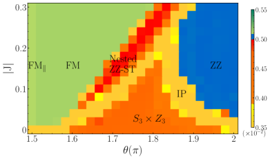
Figure 2: Machine-learned $J$-$K$-$\Gamma$ phase diagram for parameters $J<0,\ K=\sin{\theta}<0,\ \Gamma=\cos{\theta}>0$, at $T=10^{-3}$. Interactions and temperature are in units of $\sqrt{K^{2}+\Gamma^{2}}$. Each pixel represents a $(\theta,J)$ point with $\Delta\theta=\frac{1}{48}\pi$ and $\Delta J=0.02$; same for the phase diagrams below. A rank-$1$ TK-SVM with symmetric cluster of $12\times 12$ lattice cells is used. The color represents the Fiedler entry value (FEV) for the corresponding $(\theta,J)$ point, and the choice of the color bar is guided by the histogram of FEVs (Appendix B). Parameter points in the same phase have the same or very close values. The blurry regions indicate phase boundaries and crossovers. The Kitaev and $\Gamma$ spin liquids reside at the corner of $(\theta,J)=(\frac{3}{2}\pi,0)$ and $(2\pi,0)$, respectively, which are not distinguished from disordered IP regime as the rank-$1$ TK-SVM detects magnetic orders. FM: ferromagnetic, where $\text{FM}_{\parallel}$ indicates easy-axis states; Nested ZZ-ST: nested zigzag-stripy; IP: incommensurate or (correlated) paramagnetic.

Specifically, we parametrize the Kitaev and $\Gamma$ interactions as $K=\sin{\theta},\ \Gamma=\cos{\theta}$, scan over $\theta\in[\frac{3}{2}\pi,2\pi]$ and restrict the Heisenberg interaction to $J\in[-0.3,0]$. We investigate slices of experimental relevance with $J_{3}=0,0.1$ and $\Gamma^{\prime}=0,\pm 0.1$. In particular, considering a ferromagnetic as well as an anti-ferromagnetic $\Gamma^{\prime}$ covers both cases of its disputed sign in $\alpha$-${\rm RuCl}_{3}$. Most of the previous studies considered a negative $\Gamma^{\prime}$ (trigonal compression) Kim and Kee (2016); Winter et al. (2016); Eichstaedt et al. (2019); Sears et al. (2020). However, a recent work Ref. Maksimov and Chernyshev, 2020 advocates a positive $\Gamma^{\prime}$ (trigonal expansion) by stressing the electron-spin-resonance (ESR) Ponomaryov et al. (2017) and terahertz (THz) Sahasrabudhe et al. (2020) experiments, and its critical magnetic fields Cao et al. (2016); Lampen-Kelley et al. (2018); Winter et al. (2018).

We treat spins as $O(3)$ vectors to gain training data for large system sizes, corresponding to the classical large-$S$ limit. We employ parallel-tempering Monte Carlo simulations with a heat bath algorithm and over relaxation to generate spin configurations and simulate large system sizes up to $10,386$ spins ($72\times 72$ honeycomb unit cells), to accommodate potential competing orders. During the training procedure, $400$ $(\theta,J)$ points are simulated for each fixed $\Gamma^{\prime}$ and $J_{3}$ slice, and in total $2,400$ points are simulated. Training samples are collected at low temperature $T=10^{-3}\sqrt{K^{2}+\Gamma^{2}}$. Classification of these parameter points unravels the topology of the $J$-$K$-$\Gamma$ phase diagram for each of the six $\Gamma^{\prime}$ and $J_{3}$ combinations. Thereafter, we extract the physical order parameter of each phase from the learned TK-SVM decision functions. These order parameters are then measured in new simulations down to the temperature $T=10^{-4}\sqrt{K^{2}+\Gamma^{2}}$, in the most frustrated parameter regimes and passing through different phases and phase boundaries. The nature of the phases as well as the topologies of the machine-learned phase diagrams are thereby verified. See Appendix B for the setup of the sampling and training and Appendix C for details of the Monte Carlo simulations.

It turns out that the phase diagrams of the investigated parameter regions are dominated by various magnetic orders. This indicates that the classical phase diagrams may qualitatively, or even semi-quantitatively, reflect those of finite spin-$S$ values. Indeed, we successfully reproduce the ferromagnetic, zigzag and $120^{\circ}$ orders previously observed in quantum and classical analysis Rau et al. (2014); Rusnačko et al. (2019); Maksimov and Chernyshev (2020) and in addition find more phases.

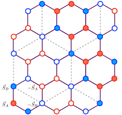
Figure 3: A ground-state configuration of the nested zigzag-stripy order. The red ($A$) and blue ($B$) colors label two inequivalent reference spins, $\vec{S}_{A}\neq\vec{S}_{B}$. The filled ($+$) and empty ($-$) cycles indicate the sign of a spin. Here the $A$-spins ($B$-spins) form zigzag (stripy) structures on a honeycomb lattice with a doubled lattice spacing. The dashed lines are a guide to the eye.

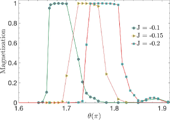
Figure 4: Monte Carlo measurements of the nested zigzag-stripy magnetization at different $J$’s, with $\Gamma^{\prime}=J_{3}=0,\ T=10^{-4}$. Consistent with the phase diagram Figure 2 learned at $T=10^{-3}$, the nested zigzag-stripy order is preferred by larger $|J|$ and $\Gamma$.

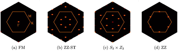
Figure 5: Evolution of the spin structure factor $S(\mathbf{q})$. The inner (outer) area denotes the first (second) honeycomb Brillouin zone; high symmetries points are indicated. Here $S(\mathbf{q})=\big{\langle}\frac{1}{2L^{2}}\sum_{ij}\mathbf{S}_{i}\cdot\mathbf{S}_{j}\,e^{i\mathbf{q}\cdot(\mathbf{r}_{i}-\mathbf{r}_{j})}\big{\rangle}$ is measured at $J=-0.1$ and $T=10^{-3}$. Upon increasing $\Gamma$, the magnetic Bragg peaks pass by the $\mathbf{\Gamma}$ (FM), $\frac{1}{2}\mathbf{M}$ (nested ZZ-ST), $\frac{2}{3}\mathbf{M}$ (modulated $S_{3}\times Z_{3}$) and $\mathbf{M}$ (zigzag) points. The length of the wave factors are stable within each phase.

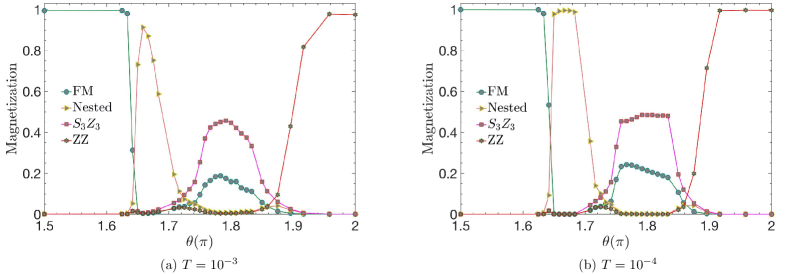
Figure 6: Monte Carlo measurements of the magnetization at fixed $J=-0.1,\ \Gamma^{\prime}=J_{3}=0$. Results for $T=10^{-3}$ and $T=10^{-4}$ are compared. The magnetic order of each phase in Figure 2 is confirmed. The broad IP regions are narrower at very low temperature $T=10^{-4}$ but remain quite sizable, indicating that these regions are highly frustrated and the orders fragile.

III $J$-$K$-$\Gamma$ Phase Diagram

We focus in this section on the machine-learned phase diagram for the pure Heisenberg-Kitaev-$\Gamma$ model and save the discussion on the effects of the $\Gamma^{\prime}$ and $J_{3}$ terms for Section IV.

The $J$-$K$-$\Gamma$ phase diagram has previously been explored by several authors; see, for example, Refs. Rau et al., 2014; Wang et al., 2019; Rusnačko et al., 2019; Chaloupka and Khaliullin, 2015. In the parameter regions with dominating Heisenberg and Kitaev exchanges, different methods give consistent results. The ferromagnetic, zigzag, anti-ferromagnetic, and stripy orders in the $J$-$K$ phase diagram Chaloupka et al. (2010); Janssen et al. (2016) extend to regions of finite $\Gamma$ Rau et al. (2014); Rusnačko et al. (2019). The physics is however more subtle when the system is governed by competing Kitaev and $\Gamma$ interactions. In the parameter regime with $K<0$, $\Gamma\sim|K|$ and a small but finite ferromagnetic $J$ term, believed to be relevant for $\alpha$-${\rm RuCl}_{3}$, a previous study based on a Luttinger-Tisza analysis suggests a zigzag order Rau et al. (2014). However, this order is not confirmed by the $24$-site exact diagonalization (ED) carried out in the same work, and a more recent study Rusnačko et al. (2019) equipped with $32$-site ED and cluster mean-field calculations shows that the physics depends on the size and shape of clusters.

Our machine finds that the phase diagram in the above parameter regime is quite rich, as shown in Figure 2. In addition to reproduce the ferromagnetic and zigzag phase in the large $K$ and $\Gamma$ regions Rau et al. (2014); Wang et al. (2019); Rusnačko et al. (2019) under a finite $J$, our machine also identifies a novel nested zigzag-stripy (ZZ-ST) phase and shows the extension of the $S_{3}\times Z_{3}$ phase. The $S_{3}\times Z_{3}$ phase results from the competition between the Kitaev and $\Gamma$ spin liquids and features a spin-orbit entangled modulation, with magnetic Bragg peaks at $\frac{2}{3}\mathbf{M}$ points Liu et al. (2021).

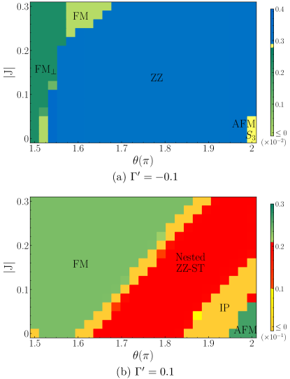
Figure 7: Machine-learned $J$-$K$-$\Gamma$ phase diagram, with $J_{3}=0,\ \Gamma^{\prime}=\pm 0.1$ at $T=10^{-3}$. A zigzag phase prevails over the phase diagram when a ferromagnetic $\Gamma^{\prime}=-0.1$ is considered, while an anti-ferromagnetic $S_{3}$ order is stabilized in the large $\Gamma$ limit. All orders in (a) are unfrustrated. By contrast, in the case of an anti-ferromagnetic $\Gamma^{\prime}$ (b), the nested zigzag-stripy phase expands significantly, and there remains a highly frustrated IP region at larger $\Gamma$ values. Panels (a) and (b) are learned with a symmetric $6\times 6$ and $4\times 4$ cluster, respectively. The resolution of $(\theta,J)$ points is same as in Fig. 2, namely, $\Delta\theta=\frac{1}{48}\pi$ and $\Delta J=0.02$. The corresponding Fiedler entries are color plotted in arbitrary unit, and their histograms are provided in Appendix B.

The nested ZZ-ST order has not been reported in previous studies to the best of our knowledge. In this phase, whose representative ground-state configuration is illustrated in Figure 3, spins can be divided into two groups, $\{\vec{S}_{A},\vec{S}_{B}\}$. One set of spins, e.g., the $A$-spins in Figure 3, form regular zigzag patterns with a doubled lattice constant while the other set of spins ($B$-spins) form stripy patterns, intricately nested with the zigzag pattern of the $A$-spins. This nesting of orders enlarges the ground-state manifold: The global three-fold rotation $(C_{3})$ and spin-inversion symmetry $(S\rightarrow-S)$ of the (generalized) $J$-$K$-$\Gamma$ model trivially allows six ground states. This degeneracy is further doubled as the two sets of spins can be swapped, leading to twelve distinct ground states, which have all been observed in our Monte Carlo simulations. In addition, the robustness of the order is also confirmed in Figure 4 by scanning $\theta$ at different $J$ values.

The formation of the $S_{3}\times Z_{3}$ and the nested ZZ-ST orders leads to an interesting evolution in spin structure factors (SSFs). As shown in Figure 5 for a fixed $J=-0.1$, in the ferromagnetic phase at small $\Gamma$, the magnetic Bragg peak develops at the $\mathbf{\Gamma}$ point of the honeycomb Brillouin zone. Increasing the $\Gamma$ coupling results in the magnetic Bragg peaks moving outwards to the $\frac{1}{2}\mathbf{M}$, $\frac{2}{3}\mathbf{M}$ and $\mathbf{M}$ points, as the system passes the nested ZZ-ST, $S_{3}\times Z_{3}$, and zigzag orders, respectively.

These phases are nonetheless separated by broad crossover areas, marked as incommensurate or paramagnetic (IP) regimes, where our machine does not detect any clear magnetic ordering down to the temperature $T=10^{-3}$. Explicit measurements of the learned order parameters at a lower temperature $T=10^{-4}$ further show all magnetic moments are indeed remarkably fragile, as plotted in Figure 6 with a fixed $J=-0.1$. Although with training data from a finite-size system and finite temperature, we cannot exclude lattice incommensuration and long-range orders at $T\rightarrow 0$ in these areas, our system size is considerably large and the absence of stable magnetic orders at such low temperatures is quite notable. One can expect quantum fluctuations will be enhanced in these areas as classical orders are suppressed, potentially hosting quantum paramagnets or spin liquids for finite spin-$S$ systems. The Kitaev and $\Gamma$ spin liquids are not distinguished from the disordered IP regimes in the phase diagram Figure 2 as the rank-$1$ TK-SVM detects only magnetic correlations. However, as we studied in Ref. Liu et al., 2021 for the $K$-$\Gamma$ model, while a classical $\Gamma$SL are less robust against competing interactions, a classical KSL can thermally extend to a finite area.

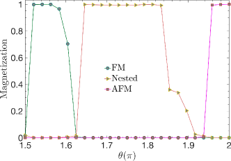
Figure 8: Monte Carlo measurements of the magnetization with fixed $J=0,\ \Gamma^{\prime}=0.1,\ J_{3}=0$, at $T=10^{-4}$. The wide window between the nested zigzag-stripy and anti-ferromagnetic orders corresponds to the IP regime in the phase diagram Figure 7 (b).

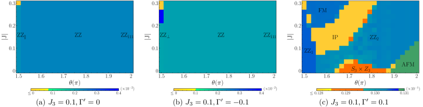
Figure 9: Machine-learned phase diagrams with $J_{3}=0.1,\,\Gamma^{\prime}=0,\,\pm 0.1$ at $T=10^{-3}$. The $J_{3}$ term universally prefers zigzag states. In cases of a vanishing and negative $\Gamma^{\prime}$, zigzag phases dominate the phase diagram, except for a narrow IP window at the $\Gamma=0$ limit with $J_{3}/J\sim-\frac{1}{3}$, which may be a remnant of a spiral order in the $J_{1}$-$J_{3}$ honeycomb model. Special zigzag states are marked in (a) and (b). With increasing $\Gamma$, the zigzag moment evolves from easy-axis ($\text{ZZ}_{\parallel}$) or coplanar directions ($\text{ZZ}_{\perp}$) to $\left<\bar{1}11\right>$ directions ($\text{ZZ}_{\bar{1}11}$) . The system is more frustrated for anti-ferromagnetic $\Gamma^{\prime}$ (c). The zigzag phase closely competes with other orders and a broad IP region. $\text{ZZ}_{1}$ and $\text{ZZ}_{2}$ distinguish different zigzag configurations. Panels (a) and (b) are learned with a symmetric $4\times 4$ cluster, and panel (c) uses a $6\times 6$ cluster. Colors reflect the value of Fiedler entries at each $(\theta,J)$ points, whose histograms are provided in Appendix B.

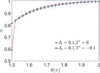
Figure 10: Evolution of the zigzag moment ($\mathbf{m}_{\rm ZZ}$) along the $J=-0.1$ line, for $J_{3}=0.1,\ \Gamma^{\prime}=0,-0.1$, at $T=10^{-3}$. Spins prefer easy-axes (easy-planes) for the case of $\Gamma^{\prime}=0$ ($\Gamma^{\prime}=-0.1$) at small $\Gamma$, but evolves towards $\mathbf{n}\in\left<\bar{1}11\right>$ with increasing $\Gamma$. $\alpha=\langle|\mathbf{m}_{\rm ZZ}\cdot\mathbf{n}|\rangle$ measures the projection of the magnetic moment on directions of $\left<\bar{1}11\right>$, and $\langle.\rangle$ denotes an ensemble average.

IV Effects of $\Gamma^{\prime}$ and $J_{3}$ term

In modeling of Kitaev materials, the inclusion of the off-diagonal $\Gamma^{\prime}$ and third-neighbor Heisenberg $J_{3}$ exchange terms can have a phenomenological motivation or a microscopic origin, as discussed in Section II. In this section, we investigate their effects on the $J$-$K$-$\Gamma$ phase diagram.

IV.1 Finite $\Gamma^{\prime}$

To disentangle their effects, we first study the case of $J_{3}=0$ and a finite $\Gamma^{\prime}$. The major consequence of adding a small ferromagnetic $\Gamma^{\prime}=-0.1$ is that the zigzag order in the $J$-$K$-$\Gamma$ phase diagram expands significantly and prevails over the phase diagram, as plotted in Figure 7 (a). In addition, a type of $120^{\circ}$ order Rau et al. (2014); Rusnačko et al. (2019) or anti-ferromagnetic $S_{3}$ order according to its order parameter structure Liu et al. (2021), which originally lives in the $K>0,\Gamma>0$ region, is induced in the corner of large $\Gamma$ and small $J$. These results are consistent with the observations in Ref. Rusnačko et al., 2019 for the quantum spin-$1/2$ model.

Our machine finds more intricate physics for the $\Gamma^{\prime}=0.1$ case. As we show in Figure 7 (b), there are three stable magnetic phases. A ferromagnet and the nested ZZ-ST magnet dominate the parameter regions of small and large $\Gamma$, respectively, while the large $\Gamma$ and small $J$ limit accommodates an anti-ferromagnet. These phases are separated by broad crossovers. In particular, as shown in Figure 8 along the $J=0$ line, in the regime between the nested and anti-ferromagnatic phase, no strong ordering is observed even down to the low-temperature $T=10^{-4}$. These regimes are hence also considered incommensurate or correlated paramagnetic (IP), similar as in the previous section for the $\Gamma^{\prime}=0$ case.

IV.2 Finite $J_{3}$ and $\Gamma^{\prime}$

We now compile all the exchange interactions together. As shown in Figure 9 (a) and (b), the anti-ferromagetic $J_{3}$ exchange term strongly favors the zigzag order regardless of a vanishing or negative $\Gamma^{\prime}$, resulting in a simple topology to the phase diagram. As measured in Figure 10, the zigzag moment prefers the directions of easy axes for $\Gamma^{\prime}=0$ and easy planes for $\Gamma^{\prime}=-0.1$ at small $\Gamma=0$, and evolves towards $\left<\bar{1}11\right>$ directions upon increasing $\Gamma$. An exception in the phase diagram is a small incommensurate or disordered area in the top left corner. This regime may be a remnant of a spiral order in the $O(3)$-symmetric $J_{1}$-$J_{3}$ honeycomb Heisenberg model Rastelli et al. (1980); Fouet et al. (2001). It is present only in a narrow window around $J_{3}/J\sim-\frac{1}{3}$ along the $\Gamma=0$ line and becomes a trivial ferromagnet at larger $|J|$.

The combination of a positive $J_{3}$ and positive $\Gamma^{\prime}$ leads to a more complex topology, as shown in Figure 9 (c). While the zigzag phase still dominates the phase diagram, the ferromagnetic and the $S_{3}\times Z_{3}$ phase, relevant for the pure $J$-$K$-$\Gamma$ model (Figure 2), and the anti-ferromagnetic phase in the vanishing $J_{3}$ but positive $\Gamma^{\prime}$ case (Figure 7), reappear. The nested ZZ-ST order, which occupied a considerable area in the $J_{3}=0$ phase diagrams, is now taken over by an IP regime and a zigzag order. Clearly, a positive $\Gamma^{\prime}$ competes with $J_{3}$ and adds frustration.

	$J$	$K$	$\Gamma$	$\Gamma^{\prime}$	$J_{3}$
$\alpha$-${\rm RuCl}_{3}$Winter et al. (2016)	$-0.97$	$-8.21$	$4.16$	$-0.93$
$\alpha$-${\rm RuCl}_{3}$Kim and Kee (2016)	$-1.67$	$-6.67$	$6.6$	$-0.87$	$2.8$
$\alpha$-${\rm RuCl}_{3}$Winter et al. (2017b)	$-0.5$	$-5.0$	$2.5$		$0.5$
$\alpha$-${\rm RuCl}_{3}$Maksimov and Chernyshev (2020)	$[-4.1,-2.1]$	$[-11,-3.8]$	$[3.9,5.0]$	[2.2,3.1]	$[2.2,3.1]$
${\rm Na}_{2}{\rm Co}_{2}{\rm TeO}_{6}$Songvilay et al. (2020)	$-0.1(8)$	$-9.0(5)$	$1.8(5)$	$0.3(3)$	$0.9(3)$
${\rm Na}_{3}{\rm Co}_{2}{\rm SbO}_{6}$Songvilay et al. (2020)	$-2.0(5)$	$-9.0(10)$	$0.3(3)$	$-0.8(2)$	$0.8(2)$

Table 1: A selection of representative microscopic interactions (in meV) proposed for three Kitaev materials. A more complete collection of models suggested for $\alpha$-${\rm RuCl}_{3}$ can be found in Refs. Laurell and Okamoto, 2020 and Maksimov and Chernyshev, 2020.

V Implication to materials

We now apply the machine-learned phase diagrams to the representative parameter sets proposed for the compounds mentioned in Section II and reproduced in Table 1.

Following the parameters given in Ref. Songvilay et al., 2020 based on inelastic neutron scattering (INS), the two cobaltate systems ${\rm Na}_{2}{\rm Co}_{2}{\rm TeO}_{6}$ and ${\rm Na}_{3}{\rm Co}_{2}{\rm SbO}_{6}$ both have a dominating ferromagnetic Kitaev exchange and a small anti-ferromagnetic $J_{3}\sim 0.1|K|$. They fall relatively deeper in the zigzag phase shown respectively in the phase diagrams of Figure 9 (a) and Figure 9 (b), in agreeement with the experimental result of Ref. Songvilay et al., 2020.

The compound $\alpha$-${\rm RuCl}_{3}$ also resides inside the zigzag phase, provided that the $\Gamma^{\prime}$ term is negligible, as suggested by the ab initio calculation and the INS fit of Ref. Winter et al., 2017b, or is negative, as suggested by the DFT calculations of Refs. Kim and Kee, 2016; Winter et al., 2016. Nevertheless, if $\Gamma^{\prime}$ is antiferromagnetic, as was recently advocated in Ref. Maksimov and Chernyshev, 2020, it falls into the far more complex phase diagram Figure 9 (c). Consistent with the linear spin-wave analysis of Ref. Maksimov and Chernyshev, 2020, the zigzag-like magnet $\alpha$-${\rm RuCl}_{3}$ will be then adjacent to an incommensurate or disordered regime.

However, it is interesting that, as indicated by Figure 2, the projection of $\alpha$-${\rm RuCl}_{3}$ on the $J$-$K$-$\Gamma$ subspace lies close to the frontier of several phases. Consider the commonly suggested range for the three major exchange interactions of this compound, $\Gamma\sim 0.5\text{--}1|K|$ ($\theta\sim 1.65\text{--}1.75\pi$), $J\sim-0.1|K|$ Winter et al. (2016); Ran et al. (2017); Kim and Kee (2016); Winter et al. (2017b); Laurell and Okamoto (2020); Maksimov and Chernyshev (2020). The relevant area in the $J$-$K$-$\Gamma$ phase diagram Figure 2 encloses, or is close to the boundary of, the $S_{3}\times Z_{3}$, the nested ZZ-ST, a ferromagnetic phase and a broad paramagnetic regime. These phases may compete with the zigzag order stabilized by a finite $\Gamma^{\prime}$ and/or $J_{3}$ term, in particular if $\Gamma^{\prime}$ is anti-ferromagnetic.

VI Summary

Kitaev materials are promising hosts of exotic phases and unconventionally ordered states of matter. Identifying the nature of those phases and constructing the associated phase diagrams is a daunting task. In this work we have utilized an interpretable and unsupervised machine-learning method, the tensorial kernel support vector machine (TK-SVM), to learn the phase diagram of a generalized Heisenberg-Kitaev-$\Gamma$ model on a honeycomb lattice.

Based on data from classical Monte Carlo simulations on large lattice size, the machine successfully reproduces the known magnetic orders as well as the incommensurate or paramagnetic-like regimes reported in the previous quantum and classical studies. It also goes further by detecting new phases in the parameter regions relevant for the compounds $\alpha$-${\rm RuCl}_{3}$, ${\rm Na}_{2}{\rm Co}_{2}{\rm TeO}_{6}$ and ${\rm Na}_{3}{\rm Co}_{2}{\rm SbO}_{6}$, including a nested zigzag-stripy phase and showing the extension of the modulated $S_{3}\times Z_{3}$ phase under finite Heisenberg interactions (Section III). In particular, the machine-learned phase diagrams suggest that, in the $J$-$K$-$\Gamma$ subspace, the actively studied compound $\alpha$-${\rm RuCl}_{3}$ is situated near the boundary of several competing phases, including a simple ferromagnet, the more involved $S_{3}\times Z_{3}$ and nested zigzag-stripy magnets, and a possibly correlated paramagnet. The inclusion of further couplings such as $\Gamma^{\prime}$ and $J_{3}$ terms stabilizes zigzag order as known in the literature. However, if the $\Gamma^{\prime}$ exchange in this material is anti-ferromagnetic and sufficiently strong to compete with $J_{3}$, as recently put forward in Ref. Maksimov and Chernyshev, 2020, the proposed parameter set will be adjacent to an incommensurate or correlated paramagnetic regime which may originate from the competition of the magnetic orders indicated above (Section IV).

To simulate large system sizes that unbiasedly accommodate different competing orders, we have treated spins as classical $O(3)$ vectors, corresponding to the large-$S$ limit of quantum spins. The fate of the novel orders identified by our machine against quantum fluctuations needs to be examined by future studies. Nevertheless, as strong symmetry-broken orders dominate, our phase diagrams can act as a useful reference for future quantum simulations. Moreover, by recognizing the unconventional orders and indicating the paramagnetic-like regimes, our phase diagrams may also guide the understanding of existing Kitaev materials and the search for new materials.

We hope our study also stimulates future machine-learning applications in Kitaev materials. While such systems are motivated by material realizations Jackeli and Khaliullin (2009); Chaloupka et al. (2010) of the Kitaev spin liquid Kitaev (2006), the presence of various non-Kitaev interactions appears to modify the physics expected from a pure Kitaev model considerably. Those interactions span a multi-dimensional parameter space, with accumulated evidence of complicated and rich phase diagrams. Machine learning techniques are designed to discover important information and structure from high-dimensional complex data and can provide new toolboxes for investigating the physics of Kitaev materials and general frustrated magnets.

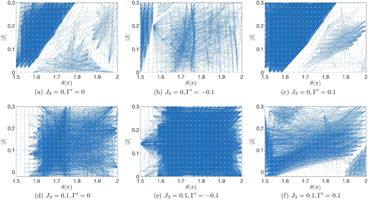
Figure 11: Graphs associated with the phase diagrams discussed in the main text. Each vertex (white circle) represents a $(\theta,J)$-point with fixed $J_{3}$ and $\Gamma^{\prime}$, from which training samples are collected. The edge (blue line) connecting two vertices is determined by the learned bias parameter $\rho$. Here $\rho_{c}=10^{4}$ is imposed in the weight function Eq. (8). Each graph contains $400$ vertices and $79,800$ edges. Edge weights are suppressed in the figure for visualization purposes.

Appendix A TK-SVM

Here we briefly review the TK-SVM method and refer to our previous work in Refs. Greitemann et al., 2019a; Liu et al., 2019; Greitemann et al., 2019b; Greitemann, 2019 for a comprehensive introduction.

A.1 Decision function

In the language of TK-SVM, a phase classification problem is solved by learning a binary decision function

$$d(\mathbf{x})=\sum_{\mu\nu}C_{\mu\nu}\phi_{\mu}(\mathbf{x})\phi_{\nu}(\mathbf{x})-\rho.$$ (4)

Here $\mathbf{x}=\{S_{i,a}\}$ represents a real-space snapshot of the system and serves as a training sample, with $i$ and $a$ respectively labeling the lattice index and component of a spin. $\bm{\phi}(\mathbf{x})$ is a feature vector mapping $\mathbf{x}$ into degree-$n$ monomials,

$$\phi^{(n)}:\mathbf{x}\rightarrow\ \bm{\phi}(\mathbf{x})=\{\phi_{\mu}\}=\{\langle S_{\alpha_{1}}^{a_{1}}S_{\alpha_{2}}^{a_{2}}\dots S_{\alpha_{n}}^{a_{n}}\rangle_{\rm cl}\},$$ (5)

where $\langle\dots\rangle_{\rm cl}$ is a lattice average over finite clusters of $r$ spins, $\mu=\{\alpha_{n},a_{n}\}$ denotes a collective index, $\alpha_{n}$ labels spins in a cluster, and the degree $n$ defines the rank of a TK-SVM kernel. The map $\phi^{(n)}$ is based on the observation that a symmetry-breaking order parameter or a local constraint for rotor degrees of freedom can be in general be represented by finite-rank tensors or polynomials Liu et al. (2016); Nissinen et al. (2016); Michel (2001). With this map, the decision function probes both linear and higher-order correlators, including magnetic order, multipolar order and ground-state constraints Greitemann et al. (2019a); Liu et al. (2019); Greitemann et al. (2019b). Moreover, this map can be combined with other machine-learning architectures, such as a principal component analysis (PCA). However, as elaborated in the thesis of J. Greitemann Greitemann (2019), it was found that TK-SVM has in general better performance and interpretability than TK-PCA. In a recent paper Ref. Miles et al., 2021, a nonlinear feature map with similar spirit was employed in a novel architecture of convolutional neural networks.

The coefficient matrix $C_{\mu\nu}$ in the decision function identifies important correlators that distinguish two data sets, from which order parameters can be extracted. It is defined as a weighted sum of support vectors,

$$C_{\mu\nu}=\sum_{k}\lambda_{k}\phi_{\mu}(\mathbf{x}^{(k)})\phi_{\nu}(\mathbf{x}^{(k)}),$$ (6)

where $\lambda_{k}$ is a Lagrange multiplier and represents the weight of the $k$-th support vector.

The bias $\rho$ in Eq. (4) is a normalization parameter in a standard SVM, but in TK-SVM it is endowed a physical implication to detect phase transitions and crossovers, or the absence thereof Liu et al. (2016); Greitemann et al. (2019b). For two sample sets $p$ and $q$, it behaves as

$$|\rho_{pq}|\begin{cases}\gg 1&\textup{${p,q}$ in the same phase},\\ \lesssim 1&\textup{${p,q}$ in different phases}.\end{cases}$$ (7)

Although the sign of $\rho$ can indicate which data set is more disordered, its absolute value suffices to construct a phase diagram; cf. Ref. Greitemann et al., 2019b for a comprehensive discussion.

The above binary classification is straightforwardly extended to a multi-classification problem over $M>1$ sets. SVM will then learn $M(M-1)/2$ binary decision functions, comprising binary classifiers for each pair of sample sets Hsu and Lin (2002).

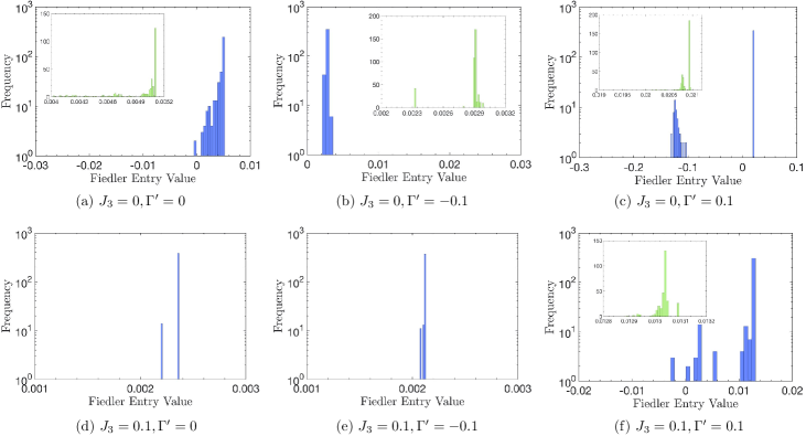
Figure 12: Histograms for the dominating Fiedler entries of the six graph partitioning problems. The main panels have a logarithmic scale on the vertical axis because the distribution spans several orders of magnitude. The insets show the main part of the distribution on a linear scale for easier comparison.

A.2 Graph partitioning

Although the standard SVM is a supervised machine-learning method Vapnik (1998), the supervision can be skipped in the TK-SVM framework thanks to multi-classification and graph partitioning.

A graph $G=(V,E)$ can be viewed as a pair of a vertex set $V$ and an edge set $E$ connecting vertices in $V$. Each vertex represents a phase point in the physical parameter space where we collect training data. For the $J$-$K$-$\Gamma$ phase diagram with fixed $\Gamma^{\prime}$ and $J_{3}$ couplings, these vertices are specified by the value of $\{\theta,J\}$. We work with weighted graphs. Namely, the edge linking two vertices $v_{p},v_{q}\in V$ has a weight $w_{pq}\in[0,1)$. Intuitively, if $v_{p},v_{q}$ are in the same phase, they will be connected with a large $w_{pq}$; otherwise $w_{pq}\simeq 0$.

The weight of an edge is determined by the bias parameter, according to its behavior given in Eq (7). The choice of the weighting function turns out not to be crucial. We adopt the normal Lorentzian weight distribution,

$$w(\rho) =1-\frac{\rho_{c}^{2}}{(|\rho|-1)^{2}+\rho_{c}^{2}}\in[0,1),$$ (8)

where $\rho_{c}$ is a hyperparameter setting a characteristic scale to quantify “$\gg 1$”. The choice of $\rho_{c}$ is uncritical and does not rely on fine tuning, as edges connecting vertices in the same phase have always larger weights than those crossing a phase boundary. In practical use, we vary $\rho_{c}$ over several orders of magnitude to ensure the results are robust. In this work, $\rho_{c}=10^{2},10^{3},10^{4}$ are considered, and $\rho_{c}=10^{4}$ is chosen to construct the graphs in Fig. 11 and the subsequent phase diagrams. We refer to our previous works Refs. Greitemann et al., 2019b and Rao et al., 2021 for comparisons of results using different $\rho_{c}$’s.

A graph of $M$ vertices and $M(M-1)/2$ edges can be represented by a $M\times M$ Laplacian matrix

$$\hat{L}=\hat{D}-\hat{A}.$$ (9)

Here, $\hat{A}$ is a symmetric off-diagonal adjacency matrix with $A_{pq}=w_{pq}$ hosting the weights of the edges. $\hat{D}$ is a diagonal degree matrix where $D_{pp}=\sum_{p\neq q}w_{pq}$ denotes the degree of vertices.

We then utilize Fiedler’s theory of spectral clustering to partition the graph $G$ Fiedler (1973, 1975), which is achieved by solving for the eigenvalues and eigenvectors of $\hat{L}$. The second smallest eigenvalue $\lambda_{2}$ reflects the algebraic connectivity of the graph, while the respective eigenvector $\mathbf{f}_{2}$ is known as the Fiedler vector. Entries of $\mathbf{f}_{2}$ have a one-to-one correspondence with vertices of the graph. Vertices (the physical parameter points) in the same subgraph will be assigned nearly identical Fiedler entries, while those in different subgraphs will be assigned contrasting values. The Fiedler vector can thereby effectively act as a phase diagram.

Appendix B Setup of the sampling and learning

The parameters specified in Section II lead to six individual problems, depending on the value of $\Gamma^{\prime}$ and $J_{3}$. For fixed $\Gamma^{\prime}$ and $J_{3}$, $400$ phase points are simulated in the $(J,\theta)$ subspace and $500$ configurations are sampled at each point. These phase points distribute uniformly in the parameter range $J\in[-0.3,0]$ and $\theta\in[1.5\pi,2\pi]$, with $\Delta J=0.02$, $\Delta\theta=\frac{1}{48}\pi$. Such a protocol of sampling does not reflect a particular strategy but just represents a natural choice when exploring unknown phase diagrams.

We perform a TK-SVM multi-classification analysis on the sampled data with different clusters and ranks in the map $\phi^{(n)}$ in Eq.(5). Each learning problem comprises $79,800$ binary decision functions, and a graph with $400$ vertices and $79,800$ edges is constructed from the learned $\rho$ parameters, as visualized in Figure 11. In all six cases, the phase diagrams can be mapped out with just rank-$1$ TK-SVMs, while a universal choice of the cluster is simply choosing a symmetric cluster with $m\times m$ honeycomb unit cells (see Figure 1). We confirm the consistency of a phase diagram by checking the results against the ones found when using larger clusters with $m=4,\,6,\,12$ ($32,\,72,\,288$ spins).

The partitioning of these graphs leads to Fiedler vectors, which reveal the topology of the phase diagrams, and are color plotted in the main text. Figure 12 shows the histograms of the Fiedler vector entires. The pronounced peaks identify well-separated phases, and the flat regions indicate disordered regimes and crossovers between the phases.

After having determined the topology of the phase diagram, the coefficient matrix $C_{\mu\nu}$ is analyzed in order to extract the order parameter for distinct phases. In cases where no magnetic order is detected, we additionally perform a rank-$2$ TK-SVM analysis and identify a phase as a spin liquid if there is a stable ground-state constraint or as a correlated paramagnet or incommensurate phase if such a constraint is absent. The learned order parameters as well as the phase diagrams are validated by additional Monte Carlo simulations in Sections III and IV.

Appendix C Simulation Details

We use parallel tempering (PT) in combination with the heat bath and over relaxation algorithms to equilibrate the system. The distribution of temperatures are carefully chosen to ensure efficient iterations between different temperatures Katzgraber et al. (2006). In the training stage, $N_{T}=64$ logarithmically equidistant temperatures between $T=0.5\times 10^{-3}$ and $10$ are used for the majority of the $(\theta,J)$ points, while $N_{T}=128$ temperatures are needed for a small subset of special parameter points. In the testing stage, $N_{T}=128$ temperatures in $[0.75\times 10^{-4},10]$ are sufficient for most points measured in Figs. 6, 4 and 8, but $N_{T}=256$ temperatures are required for a few points.

We typically run $8\times 10^{6}$ Monte Carlo (MC) sweeps for simulations using $N_{T}=64$ and $1.6\times 10^{7}$ sweeps for those requiring more temperatures. Half of the total sweeps are considered as thermalization. In the training stage, $500$ samples are collected from the second half of simulations. Namely, the sampling interval is $800$ or $1,600$ MC sweeps. In the testing stage, new Monte Carlo simulations are performed to measure the learned order parameters (Figs. 6, 4 and 8), and several independent simulations are compared to confirm the ergodicity and good thermalization of our simulations. Alternatively, one could also measure the learned decision functions (without interpretation) as in applications of a standard SVM. As we established in Refs. Greitemann et al., 2019a; Liu et al., 2019, the TK-SVM decision function is essentially an encoder of physical order parameters. However, the goal of machine-learned phase diagrams is to not only to assign each phase a different label but also to find suitable characterizations of the phases. Direct measurements of physical quantities are hence preferred if interpretability is guaranteed.

References

- Carleo et al. (2019) Giuseppe Carleo, Ignacio Cirac, Kyle Cranmer, Laurent Daudet, Maria Schuld, Naftali Tishby, Leslie Vogt-Maranto, and Lenka Zdeborová, “Machine learning and the physical sciences,” Rev. Mod. Phys. 91, 045002 (2019).
- Mehta et al. (2019) Pankaj Mehta, Marin Bukov, Ching-Hao Wang, Alexandre G.R. Day, Clint Richardson, Charles K. Fisher, and David J. Schwab, “A high-bias, low-variance introduction to Machine Learning for physicists,” Physics Reports 810, 1 – 124 (2019), a high-bias, low-variance introduction to Machine Learning for physicists.
- Wang (2016) Lei Wang, “Discovering phase transitions with unsupervised learning,” Phys. Rev. B 94, 195105 (2016).
- Ponte and Melko (2017) Pedro Ponte and Roger G. Melko, “Kernel methods for interpretable machine learning of order parameters,” Phys. Rev. B 96, 205146 (2017).
- Carrasquilla and Melko (2017) Juan Carrasquilla and Roger G. Melko, “Machine learning phases of matter,” Nat. Phys. 13, 431–434 (2017).
- Chen et al. (2020) Li Chen, Xiao Liang, and Hui Zhai, “The bayesian committee approach for computational physics problems,” (2020), arXiv:2011.06086 [physics.comp-ph] .
- Carleo and Troyer (2017) Giuseppe Carleo and Matthias Troyer, “Solving the quantum many-body problem with artificial neural networks,” Science 355, 602–606 (2017).
- Carrasquilla (2020) Juan Carrasquilla, “Machine learning for quantum matter,” Advances in Physics: X 5, 1797528 (2020).
- Deng et al. (2017) Dong-Ling Deng, Xiaopeng Li, and S. Das Sarma, “Quantum entanglement in neural network states,” Phys. Rev. X 7, 021021 (2017).
- Hermann et al. (2020) Jan Hermann, Zeno Schätzle, and Frank Noé, “Deep-neural-network solution of the electronic Schrödinger equation,” Nature Chemistry 12, 891–897 (2020).
- Pfau et al. (2020) David Pfau, James S. Spencer, Alexander G. D. G. Matthews, and W. M. C. Foulkes, “Ab initio solution of the many-electron Schrödinger equation with deep neural networks,” Phys. Rev. Research 2, 033429 (2020).
- Vieijra et al. (2020) Tom Vieijra, Corneel Casert, Jannes Nys, Wesley De Neve, Jutho Haegeman, Jan Ryckebusch, and Frank Verstraete, “Restricted boltzmann machines for quantum states with non-abelian or anyonic symmetries,” Phys. Rev. Lett. 124, 097201 (2020).
- Nussinov et al. (2016) Z. Nussinov, P. Ronhovde, Dandan Hu, S. Chakrabarty, Bo Sun, Nicholas A. Mauro, and Kisor K. Sahu, “Inference of hidden structures in complex physical systems by multi-scale clustering,” in Information Science for Materials Discovery and Design, edited by Turab Lookman, Francis J. Alexander, and Krishna Rajan (Springer International Publishing, Cham, 2016) pp. 115–138.
- Zhang et al. (2019) Yi Zhang, A. Mesaros, K. Fujita, S. D. Edkins, M. H. Hamidian, K. Ch’ng, H. Eisaki, S. Uchida, J. C. Séamus Davis, Ehsan Khatami, and Eun-Ah Kim, “Machine learning in electronic-quantum-matter imaging experiments,” Nature 570, 484–490 (2019).
- Bohrdt et al. (2019) Annabelle Bohrdt, Christie S. Chiu, Geoffrey Ji, Muqing Xu, Daniel Greif, Markus Greiner, Eugene Demler, Fabian Grusdt, and Michael Knap, “Classifying snapshots of the doped Hubbard model with machine learning,” Nature Physics 15, 921–924 (2019).
- Schmidt et al. (2019) Jonathan Schmidt, Mário R. G. Marques, Silvana Botti, and Miguel A. L. Marques, “Recent advances and applications of machine learning in solid-state materials science,” npj Computational Materials 5, 83 (2019).
- Liao et al. (2019) Hai-Jun Liao, Jin-Guo Liu, Lei Wang, and Tao Xiang, “Differentiable programming tensor networks,” Phys. Rev. X 9, 031041 (2019).
- Liu et al. (2017) Junwei Liu, Yang Qi, Zi Yang Meng, and Liang Fu, “Self-learning monte carlo method,” Phys. Rev. B 95, 041101 (2017).
- Takagi et al. (2019) Hidenori Takagi, Tomohiro Takayama, George Jackeli, Giniyat Khaliullin, and Stephen E. Nagler, “Concept and realization of Kitaev quantum spin liquids,” Nat. Rev. Phys. 1, 264–280 (2019).
- Janssen and Vojta (2019) Lukas Janssen and Matthias Vojta, “Heisenberg-Kitaev physics in magnetic fields,” J. Phys.: Condens. Matter 31, 423002 (2019).
- Winter et al. (2017a) Stephen M Winter, Alexander A Tsirlin, Maria Daghofer, Jeroen van den Brink, Yogesh Singh, Philipp Gegenwart, and Roser Valentí, “Models and materials for generalized Kitaev magnetism,” Journal of Physics: Condensed Matter 29, 493002 (2017a).
- Kitaev (2006) Alexei Kitaev, “Anyons in an exactly solved model and beyond,” Ann. Phys. (N. Y.) 321, 2–111 (2006), january Special Issue.
- Jackeli and Khaliullin (2009) G. Jackeli and G. Khaliullin, “Mott Insulators in the Strong Spin-Orbit Coupling Limit: From Heisenberg to a Quantum Compass and Kitaev Models,” Phys. Rev. Lett. 102, 017205 (2009).
- Chaloupka et al. (2010) J. Chaloupka, George Jackeli, and Giniyat Khaliullin, “Kitaev-Heisenberg Model on a Honeycomb Lattice: Possible Exotic Phases in Iridium Oxides ,” Phys. Rev. Lett. 105, 027204 (2010).
- Banerjee et al. (2016) A. Banerjee, C. A. Bridges, J. Q. Yan, A. A. Aczel, L. Li, M. B. Stone, G. E. Granroth, M. D. Lumsden, Y. Yiu, J. Knolle, S. Bhattacharjee, D. L. Kovrizhin, R. Moessner, D. A. Tennant, D. G. Mandrus, and S. E. Nagler, “Proximate Kitaev quantum spin liquid behaviour in a honeycomb magnet,” Nat. Mater. 15, 733–740 (2016).
- Banerjee et al. (2017) Arnab Banerjee, Jiaqiang Yan, Johannes Knolle, Craig A. Bridges, Matthew B. Stone, Mark D. Lumsden, David G. Mandrus, David A. Tennant, Roderich Moessner, and Stephen E. Nagler, “Neutron scattering in the proximate quantum spin liquid ,” Science 356, 1055–1059 (2017).
- Ran et al. (2017) Kejing Ran, Jinghui Wang, Wei Wang, Zhao-Yang Dong, Xiao Ren, Song Bao, Shichao Li, Zhen Ma, Yuan Gan, Youtian Zhang, J. T. Park, Guochu Deng, S. Danilkin, Shun-Li Yu, Jian-Xin Li, and Jinsheng Wen, “Spin-Wave Excitations Evidencing the Kitaev Interaction in Single Crystalline ,” Phys. Rev. Lett. 118, 107203 (2017).
- Yadav et al. (2016) Ravi Yadav, Nikolay A. Bogdanov, Vamshi M. Katukuri, Satoshi Nishimoto, Jeroen van den Brink, and Liviu Hozoi, “Kitaev exchange and field-induced quantum spin-liquid states in honeycomb ,” Scientific Reports 6, 37925 (2016).
- Yadav et al. (2019) Ravi Yadav, Satoshi Nishimoto, Manuel Richter, Jeroen van den Brink, and Rajyavardhan Ray, “Large off-diagonal exchange couplings and spin liquid states in -symmetric iridates,” Phys. Rev. B 100, 144422 (2019).
- Chaloupka and Khaliullin (2015) J. Chaloupka and G. Khaliullin, “Hidden symmetries of the extended Kitaev-Heisenberg model: Implications for the honeycomb-lattice iridates ,” Phys. Rev. B 92, 024413 (2015).
- Kasahara et al. (2018) Y. Kasahara, T. Ohnishi, Y. Mizukami, O. Tanaka, Sixiao Ma, K. Sugii, N. Kurita, H. Tanaka, J. Nasu, Y. Motome, T. Shibauchi, and Y. Matsuda, “Majorana quantization and half-integer thermal quantum hall effect in a Kitaev spin liquid,” Nature 559, 227–231 (2018).
- Yokoi et al. (2020) T Yokoi, S Ma, Y Kasahara, S Kasahara, T Shibauchi, N Kurita, H Tanaka, J Nasu, Y Motome, C Hickey, S. Trebst, and Y. Matsuda, “Half-integer quantized anomalous thermal Hall effect in the Kitaev material ,” arXiv preprint arXiv:2001.01899 (2020).
- Ponomaryov et al. (2020) A. N. Ponomaryov, L. Zviagina, J. Wosnitza, P. Lampen-Kelley, A. Banerjee, J.-Q. Yan, C. A. Bridges, D. G. Mandrus, S. E. Nagler, and S. A. Zvyagin, “Nature of Magnetic Excitations in the High-Field Phase of ,” Phys. Rev. Lett. 125, 037202 (2020).
- Sahasrabudhe et al. (2020) A. Sahasrabudhe, D. A. S. Kaib, S. Reschke, R. German, T. C. Koethe, J. Buhot, D. Kamenskyi, C. Hickey, P. Becker, V. Tsurkan, A. Loidl, S. H. Do, K. Y. Choi, M. Grüninger, S. M. Winter, Zhe Wang, R. Valentí, and P. H. M. van Loosdrecht, “High-field quantum disordered state in : Spin flips, bound states, and multiparticle continuum,” Phys. Rev. B 101, 140410 (2020).