REvolver
Automated running and matching of couplings and masses in QCD

Abstract

In this article we present REvolver, a C++ library for renormalization group evolution and automatic flavor matching of the QCD coupling and quark masses, as well as precise conversion between various quark mass renormalization schemes. The library systematically accounts for the renormalization group evolution of low-scale short-distance masses which depend linearly on the renormalization scale and sums logarithmic terms of high and low scales that are missed by the common logarithmic renormalization scale evolution. The library can also be accessed through Mathematica and Python interfaces and provides renormalization group evolution for complex renormalization scales as well.

UWThPh-2020-18, IFT-UAM/CSIC-21-5

PROGRAM SUMMARY

Program Title: REvolver
Licensing provisions: GPLv3 or later
Programming language: C++, Python, Wolfram Language
Program obtainable from: https://gitlab.com/REvolver-hep/REvolver
Operating system: Linux, MacOS, partially Windows
Required RAM: insignificant for a limited number of instances of the Core class
Number of processors used: one
Running time: fractions of seconds for single commands
Supplementary material: this article, demo programs, doxygen documentation

Nature of problem:
The strong coupling and the quark masses are fundamental parameters of QCD that are scheme and renormalization-scale dependent. The choice of scheme depends on the active number of flavors and the range of scales, and is dictated by the requirements to minimize the size of corrections and to sum large logarithmic corrections to all orders. For the strong coupling and the quark masses at high scales, the $\overline{\mbox{MS}}$ scheme with logarithmic scale dependence is used. For quark masses at low scales, short-distance mass schemes with linear scale-dependence are used. The REvolver library provides conversions for the strong coupling and the most common quark mass schemes, with renormalization scale evolution implemented such that all types of large logarithmic terms are summed to all orders, accounting for flavor threshold effects and state-or-the-art correction terms. The pole mass, which is not a short-distance mass and contains a sizable renormalon ambiguity, is treated as a derived quantity.

Solution method:
Renormalization group equations are solved for complex-valued scales to machine precision based on fast-converging iterative algorithms and analytic all-order expressions. Matching relations for the strong coupling at flavor thresholds are computed in a way that gives equal results for upward and downward evolution. Core objects allow to define an arbitrary number of physical scenarios for strong coupling values and quark mass spectra, where options for precision and matching scales can be set freely, and values for quark masses in all common schemes including the pole mass can be extracted. All REvolver routines are implemented entirely in C++ and can be accessed through Mathematica and Python interfaces.

1 Introduction

Quark masses are fundamental parameters of quantum chromodynamics(QCD) and their precise determination in adequate schemes and at appropriate renormalization scales is of high interest for theoretical as well as experimental studies of many processes. These can be governed by energy scales ranging from a few GeV (e.g. for hadronic states) up to several hundred GeV and even TeV scales (e.g. for particle collisions that take place at the Large Hadron Collider). One needs to employ the renormalization group evolution equations to reliably relate the values of quark masses defined at such widely different energy scales. An interesting situation arises if the dynamical scale governing the quark mass dependence of an observable is much smaller than the quark mass itself. In this case, the common running ${\overline{\rm MS}}$ mass scheme, which obeys a renormalization group equation with logarithmic scale dependence, cannot be employed for high-precision applications, because it is only meaningful for scales of the order or larger than the mass. Rather, so-called low-scale short-distance masses must be used, which obey renormalization group equations with linear scale dependence. The numerical impact of the renormalization group evolution is particularly important for the top quark mass where, due to its large value, significant scale hierarchies can arise.

Here we present REvolver, a C++ library with routines that provide renormalization-group resummed conversions between quark mass schemes defined at different renormalization scales, including scales much lower than the mass, where low-scale short-distance masses are employed, as well as above the mass value, where the ${\overline{\rm MS}}$ mass is used. The routines are based on the creation of so-called Core objects, each of which representing a certain physical scenario for the heavy quark masses (charm, bottom and top quarks, as well as hypothetical heavier flavors), the number of massless quarks and the strong coupling $\alpha_{s}$. In a single session, an (in principle) arbitrary number of Core objects can be created and managed. Each Core object can then provide values for the quark masses in the most popular low-scale short-distance schemes as well as for the ${\overline{\rm MS}}$ mass and the strong coupling at any (real or complex-valued) renormalization scale and in any flavor number scheme, consistently accounting for flavor threshold effects and the resummation of large logarithms of all kinds. The basis of the quark mass evolution equations for scales below the respective mass is the renormalization group equation of the natural MSR mass (here simply called the MSR mass), which was provided in Refs. [1] together with a full treatment of flavor matching corrections when the evolution crosses the thresholds related to lighter massive quarks [2]. Furthermore, for each Core object, options can be set to specify the perturbative precision in the flavor matching and the renormalization group evolution. Using all available theoretical input in the literature, see Sec. 8 for a detailed listing, it is possible to relate the ${\overline{\rm MS}}$, MSR and most other low-scale short-distance quark masses with a theoretical precision of $10$ to $20$ MeV (neglecting any parametric uncertainties). Quark mass values in the pole scheme cannot be defined at the same level of precision due to the pole mass renormalon ambiguity which decreases the accuracy by an order of magnitude [3, 2]. REvolver offers the possibility to set up Core objects using pole masses as an input or to extract pole mass values from a Core object, but it treats the pole mass as a derived quantity where the user has to specify the way in which the pole mass value is defined. Furthermore, REvolver provides various options to account for the asymptotic higher order corrections of the pole mass and the pole mass renormalon ambiguity. All REvolver routines are implemented entirely in C++ and can be accessed through Mathematica and Python interfaces.

There is an existing C++ library accompanied by a Mathematica package called CRunDec and RunDec [4, 5], respectively, which already provide many functionalities included in the REvolver library. We have cross checked in detail that any theoretical (perturbative) input implemented in CRunDec and RunDec agrees with the corresponding one employed for REvolver. We have furthermore checked that the numerical output of the routines provided in CRunDec/RunDec is in agreement with the equivalent routines of REvolver. The REvolver library, however, exceeds CRunDec/RunDec

• by providing the Core concept that allows to automatically create, extend and manage an arbitrary number of scenarios for strong coupling values, mass spectra and theory settings, and to extract quark masses and the QCD coupling in all flavor number schemes and at all scales,

• by accounting for the renormalization group resummation of large logarithms and lighter massive quark flavor thresholds when dealing with quark masses at renormalization scales smaller than the quark mass, as well as for low-scale short-distance masses,

• by giving access to machine-precision numerical routines that provide quasi-exact solutions of the renormalization group equations for the running masses and the strong coupling at complex scales, and

• by providing routines to determine the asymptotic series for the pole mass to an arbitrary order that allow to extract different pole mass definitions and to quantify the pole mass renormalon ambiguity with various methods.

The emphasis of all REvolver functionalities is to provide integrated and easy-to-use routines, while maintaining the possibility to deviate from default settings and specify all available options, useful for high-precision phenomenological and conceptual QCD studies aiming for uncertainties at the level of $10$ to $20$ MeV for short-distance masses.

This article is organized as follows: In Sec. 2 essential terminology used for the description of the REvolver package is explained. In Sec. 3 we succinctly review the MSR mass and the R-evolution concepts [1, 6] which are essential for the resummation of the logarithms mentioned above in bullet point (ii). Section 4 provides general information concerning the REvolver installation and setting up the C++, Mathematica and Python interfaces. The philosophy of the Core concept is explained in Sec. 5, and Sec. 6 provides a structured introduction to all available REvolver routines. In Sec. 7 a sizable number of pedagogical examples for applications of REvolver routines are provided, partly using the routine’s default settings, partly using alternative optional parameter setting, to demonstrate the versatility of REvolver for important phenomenological applications in the literature. It is recommended that the user consults the examples shown in this section, which are also collected in a Mathematica notebook, a Jupyter Notebook using the Python interface, and a C++ source file provided with the REvolver package. In Sec. 8 important references are provided which were used as the source for the higher order corrections implemented for the strong coupling and the mass schemes supported by REvolver. Here, also a detailed citation recommendation for these higher order corrections is provided. Section 9 contains a summary. Finally, some details concerning the algorithms used for Core creation and the quasi-exact solution of renormalization group equations are given in Appendix A. In addition, a number of essential formulae for implementation-dependent quantities are provided which cannot be found in the literature in the form used in REvolver.

2 Terminology

This article employs a particular terminology when referring to renormalization-scale dependent mass schemes and the pole mass:

• Running quark mass in the $n_{f}$-flavor scheme $m^{(n_{f})}_{q}(\mu)$: Refers to the $\overline{\mathrm{MS}}$ mass if the flavor number $n_{f}$ includes this massive quark, and the MSR mass otherwise. For example, the running top quark mass at the scale $\mu$ in the 6-flavor scheme $m_{t}^{(6)}(\mu)$ refers to the $\overline{\mathrm{MS}}$ mass $\overline{m}_{t}^{(6)}(\mu)$, and the running top quark mass at the scale $\mu$ in the 4-flavor scheme $m_{t}^{(4)}(\mu)$ refers to the MSR mass $m_{t}^{{\rm MSR},(4)}(\mu)$.

• Standard running mass $\overline{m}_{q}$: Refers to the $\overline{\mathrm{MS}}$ mass in the flavor number scheme where all lighter quarks along with this quark are treated dynamically, evaluated at the scale of this mass. For example, the standard running top mass is the $6$-flavor $\overline{\mathrm{MS}}$ quark mass evaluated at the scale of this top mass: $\overline{m}_{t}\equiv\overline{m}_{t}^{(6)}\!(\overline{m}_{t}^{(6)})$. The mass dependence of all flavor-threshold corrections is expressed in terms of the standard running mass.

• Asymptotic pole mass: Refers to the pole mass value obtained from the running mass defined by summing the perturbative series to the order of the minimal correction.

• Order-dependent pole mass: Refers to the pole mass value obtained from the running mass by truncating the perturbative series at a specified order.

3 The MSR mass and R-evolution

The natural MSR mass of a massive quark defined in Ref. [1] (and called just the MSR mass here) plays a central role in REvolver and is a renormalization scale and flavor-number-dependent low-scale short-distance mass. It is derived from the $\overline{\mathrm{MS}}$ mass and treated as the natural extension of the $\overline{\mathrm{MS}}$ mass for renormalization scales below the mass of the quark. This combination of the scale-dependent $\overline{\mathrm{MS}}$ and MSR masses extends the well known concept of flavor-number dependent renormalization group evolution and flavor threshold matching for scales above the quark mass (where the $\overline{\mathrm{MS}}$ mass scheme is appropriate) to lower scales. In contrast to usual logarithmic renormalization scale evolution (as known from the $\overline{\mathrm{MS}}$ masses or the strong coupling), the MSR mass renormalization group evolution is linear. This is consequence of the linear dynamical scaling that arises when the off-shell massive quark quantum fluctuations are integrated out in the nonrelativistic limit. Together with the flavor number dependent strong $\overline{\mathrm{MS}}$ coupling, the $\overline{\mathrm{MS}}$ and MSR masses form the basis of the core concept of REvolver and allow to also resum large logarithms involving low-scale short-distance mass schemes other than the MSR mass. This functionality is used by default in the REvolver routines (but can also be switched off by the user on demand). The MSR mass [1, 2, 6] has already been used in a number of applications, but we still find it warranted to briefly review its main concepts in this section. For simplicity, we consider the case in which all $n_{\ell}$ quarks lighter than $q$ are massless. The reader is referred to Ref. [2] for the case with massive lighter quarks.

To define the MSR mass, one starts with the relation between the standard running mass and pole mass,

$$m_{q}^{\rm pole}-\overline{m}_{q}=\overline{m}_{q}\,\sum_{n=1}^{\infty}\,a_{n}^{\overline{\rm MS}}(n_{\ell},n_{h})\Biggl{[}\frac{\alpha_{s}^{(n_{\ell}+n_{h})}(\overline{m}_{q})}{4\pi}\Biggr{]}^{\!n}\,,$$ (1)

where $n_{f}=n_{\ell}+n_{h}$ is the number of active flavors, with $n_{\ell}$ being the number of massless quarks and $n_{h}=1$ referring to the quark $q$. Since the MSR mass is employed for renormalization scales below $m_{q}$, one integrates out the virtual heavy quark loops by setting $n_{h}=0$. This allows to define a renormalization scale $R$ smaller than $m_{q}$ and the corrections to the pole mass having a linear dependence on $R$ to implement a consistent nonrelativistic scaling behavior. The MSR mass is thus defined by furthermore setting $\overline{m}_{q}\to R$:

$$m_{q}^{\rm pole}-m_{q}^{{\rm MSR},(n_{\ell})}(R)=R\sum_{n=1}^{\infty}a_{n}^{\overline{\mathrm{MS}}}(n_{\ell},0)\!\Biggl{[}\frac{\alpha_{s}^{(n_{\ell})}(R)}{4\pi}\Biggr{]}^{\!n}\,.$$ (2)

In contrast to the $\overline{\mathrm{MS}}$ mass, which has only logarithmic dependence on the scale $\mu$, the MSR mass has an additional linear dependence on $R$. The $\overline{\mathrm{MS}}$ and MSR masses can be related perturbatively and unambiguously through Eqs. (1) and (2) because the pole mass in both equalities is identical. The resulting perturbative series for the difference of two MSR masses at different renormalization scales $R_{1}$ and $R_{2}$ is renormalon free, as long as it is expressed in powers of the strong coupling at the same renormalization scale. As a result, for disparate values of $R_{1}$ and $R_{2}$ large logarithms will appear. These logarithms can be consistently summed up with the renormalization group equation

$$-\!\frac{\rm d}{{\rm d}R}m_{q}^{{\rm MSR},(n_{\ell})}(R)=\gamma_{R}^{M}[\alpha_{s}^{(n_{\ell})}(R)]=\sum_{n=0}^{\infty}\gamma_{n}^{R}(n_{\ell})\!\Biggl{[}\frac{\alpha_{s}^{(n_{\ell})}(R)}{4\pi}\Biggr{]}^{\!n+1},$$ (3)

In contrast to the logarithmic renormalization group equations for the $\overline{\mathrm{MS}}$ mass and the strong coupling, it shows a linear power scaling and has therefore been dubbed as the R-evolution equation. The anomalous dimension coefficients $\gamma_{n}^{R}(n_{\ell})$ can be calculated from the relation [ see Eq. (6) for the definition of the QCD $\beta$-function coefficients $\beta_{i}$ ]

$$\gamma_{n}^{R}(n_{\ell})=a^{\overline{\mathrm{MS}}}_{n+1}(n_{\ell},0)-2\sum_{j=0}^{n-1}(n-j)\,\beta_{j}\,a^{\overline{\mathrm{MS}}}_{n-j}(n_{\ell},0)\,.$$ (4)

The coefficients of the R-evolution equation have the following explicit form:

$$\gamma_{0}^{R}(n_{\ell}) ={\textstyle\frac{16}{3}}\,,$$ (5)

$$\gamma_{1}^{R}(n_{\ell}) =96.1039-9.55076\,n_{\ell}\,,$$

$$\gamma_{2}^{R}(n_{\ell}) =1595.75-269.953\,n_{\ell}-2.65945\,n_{\ell}^{2}\,,$$

$$\gamma_{3}^{R}(n_{\ell}) =(12319.\pm 417.)-(9103.\pm 10.)\,n_{\ell}+610.264\,n_{\ell}^{2}-6.515\,n_{\ell}^{3}\,.$$

The uncertainties in the ${\cal O}(\alpha_{s}^{4})$ coefficient arise from the numerical uncertainties in the relation between the $\overline{\mathrm{MS}}$ and the pole masses at this order. In App. A.4 we present an efficient algorithm to exactly integrate Eq. (3).

Adopting appropriate values for $R$ and $n_{\ell}$ the MSR mass $m_{q}^{{\rm MSR},(n_{\ell})}(R)$ can be related in a renormalon-free manner to any other low-scale short-distance mass without the appearance of large logarithms and can thus be used to also resum potentially large R-evolution logarithms in the relation of other low-scale short-distance mass schemes. In the presence of massive quarks with masses lighter than $m_{q}$, the MSR mass has an $n_{\ell}$-dependent renormalization group evolution and flavor threshold corrections in close analogy to the renormalization group evolution of the strong coupling and the $\overline{\mathrm{MS}}$ mass. This allows for the resummation of large logarithms involving the masses of the lighter massive quarks. For details we refer to Ref. [2].

4 Setup

There are three ways to access the functionalities of the REvolver library:

• via the C++ library directly, which might be most suitable for extensive automated tasks and to interface with other libraries and codes,

• via the Wolfram Mathematica [7] interface (using WSTP / MathLink), which is suitable for interactive tasks and for using in parallel with other Mathematica features,

• via the Python [8] interface (generated using SWIG [9]) for usage in scripts and interactive execution in Jupyter notebooks [10].

4.1 Installation

Note that slightly more detailed instructions for installing the code, including Windows-specific commands, are given in the README.md file provided with the source code. Here we only describe the installation procedure for Linux and MacOS, and only for REvolver itself (not for CMake and other auxiliaries).

For the compilation of REvolver a C++11 compatible compiler is needed. The recommended (and tested) choices are gcc on Linux, Apple Clang on MacOS and MinGW on Windows. It is expected that REvolver compiles on other platforms and with different compilers as well, although this has not been tested and we do not provide any specific instructions.

We provide a CMake script with various options controlling which interfaces and demonstration codes are built. To use the script, at least version 3.1 of CMake is required.

If REvolver is to be used via Mathematica, Wolfram Mathematica is required in a version which supports WSTP or MathLink.

For the Python interface, at least version 3 of Python has to be installed, including the development packages. We note that the Python interface is currently supported only on Linux and MacOS.

After downloading the code to the local hard drive, open a command line interface, navigate to the directory code/ and run the commands

  $ mkdir build
  $ cd build/

In the next step, the CMake script will be executed. Depending on which interfaces are to be prepared, various flags can be set:

• wolfr determines if the Mathematica interface is prepared (default: OFF),

• py determines if the Python interface is prepared (default: OFF),

• cpp_demo determines if the C++ demo executable is built (default: ON).

The static REvolver C++ library is always compiled. Note that to compile the C++ demo executable the library Quadpack++ [11] is used. However, no additional steps are required by the user since the library is provided with REvolver. Note that the Quadpack++ library is only compiled if the flag cpp_demo is set to ON.

To execute the CMake script with default flags and compile the code, one has to run the terminal commands

  $ cmake ..
  $ make install

or in general

  $ cmake [(-D <flag>={ON|OFF})...] ..
  $ make install

where <flag> is a placeholder for one of the flags listed above. For example, to prepare the Mathematica interface, but not the compilation of the C++ demo code one would use

  $ cmake -D wolfr=ON -D cpp_demo=OFF ..
  $ make install

The directory code/build/ can be safely removed after the compiling is done. The resulting libraries and executables can be found at the following locations:

• the static C++ library file:
  code/lib/libREvolver.a

• the MathLink / WSTP executable, ready to be loaded in a Mathematica notebook:
  code/bin/REvolver

• the Python module file and dynamic library, ready to be imported in a Python script:
  code/pyREvolver/lib/pyREvolver.py
  code/pyREvolver/lib/_pyREvolver.so

• the C++ demo executable:
  code/bin/examples

4.2 General Usage

C++ Interface

To use the REvolver C++ static library, the respective header file has to be included which is done via

  #include REvolver.h

and the library has to be properly linked when compiling the code. After including the header file, the implemented classes and routines are available in the namespace revo and accessible with the scope resolution prefix revo:: unless the instruction using namespace revo; has been invoked, such that the resolution prefix is not necessary.

For a demonstration, we refer to the source file code/examples/examples.cpp and the related executable code/bin/examples (if cpp_demo=ON was set).

Mathematica Interface

To load the WSTP executable in a Mathematica notebook, execute

  Install["<path to executable>/REvolver"]

with <path to executable> referring to the directory path where the executable is located. For future convenience it might be useful to execute

  CopyFile["<path to executable>/REvolver",
           $UserBaseDirectory <> "/Applications/REvolver"]

which copies the executable to the user base directory of Mathematica, making it possible to load the executable with the command

  Install["REvolver"]

in the future.

For a demonstration of how to load REvolver in a Mathematica notebook and a general overview of the available functions, see the demonstration notebook code/examples/examples.nb provided with the package.

Python Interface

The module can be loaded in a Python script or Jupyter notebook with the usual syntax

  import pyREvolver

assuming that pyREvolver.py and the shared library file (*.so) are located in the same folder as the script or notebook, or have been added to the module search path with the following command

  import sys
  sys.path.append(’<path to pyREvolver.py>’)

For a demonstration of how to load and use the module, see the Jupyter notebook code/examples/examples.ipynb provided with the package.

5 Core Structure

As described in the introduction, all functionalities of the library are centered around instances of the class revo::Core (simply called “Core objects” or “Cores” in the following) each representing a certain physical scenario for the quark mass spectrum and the strong coupling and from which numerical values for quark masses and the strong coupling in specified schemes and at specified scales can be extracted. In principle, the number of Core objects defined at the same time is only limited by the available memory, regardless of the interface used.

Figure 1: Schematic structure of the class revo::Core in C++: the class contains an instance of the class revo::Alpha as a member providing functionalities related to the strong coupling such as running and matching, and an instance of the class revo::Mass providing functionalities related to the quark masses such as running, matching and conversion. revo::Mass uses revo::Alpha for coupling evolution, and revo is the namespace where all relevant REvolver classes are defined.

The schematic structure of the class revo::Core in C++ is depicted in Fig. 1: the class has objects of the classes revo::Alpha and revo::Mass as members. The class revo::Alpha has various member functions related to the strong coupling like running, matching and for obtaining the QCD scale $\Lambda_{\mathrm{QCD}}$. The class revo::Mass has member functions related to the evolution and matching of the running masses as well as the extraction of quark mass values in specified schemes. It uses an instance of the class revo::Alpha to obtain the necessary coupling values. The respective member objects of the revo::Core class can be accessed through the member functions revo::Core::alpha() and revo::Core::masses(), respectively. The class revo::Core itself represents the frame to access these member functions and provides additional functionalities related to setting up a physical coupling and quark mass spectrum scenario, and extending an existing scenario by adding additional heavier massive quarks.

Although in principle possible, helper classes such as revo::Mass and revo::Alpha are not meant to be used outside Core objects. All available functionalities can (and should) be accessed through Core objects.

When using the Mathematica interface, the specific structure of the classes are not relevant since the wrapper hides most details to fit into the Wolfram language syntax. To preserve the possibility to have multiple Cores defined at the same time in Mathematica, a unique name has to be specified for each Core instance, which is referred to when extracting mass and coupling values or when extending scenarios.

For concrete usage and examples we refer to Secs. 6 and 7.

6 Implemented Functions

In the following descriptions and examples we will assume that the namespace revo has been introduced in the C++ code with the instruction

  using namespace revo;

such that the scope resolution prefix revo:: can be omitted, and that in Python the module was loaded with

  from pyREvolver import *

to keep code snippets uncluttered.

The syntax and interface structure in Python is the same as in C++, with a few exceptions:

• If a constant of an enum class type has to be provided as an input, the scope resolution operator :: has to be exchanged with _, e.g. the enumerator MSbar of type MScheme has to be provided using MScheme_MSbar instead of MScheme::MSbar.

• The C++ function Mass::mPole allows for two optional pointer-type inputs to provide the possibility of accessing several output values (see Sec. 6.2.3). In Python, instead, within the class Mass the additional member function mPoleDetailed is provided which returns a tuple of values. In Mathematica the same functionality is provided by the function MassPoleDetailed.

• C++ specific syntax cannot be used, e.g. initializing an std::vector with an initializer list.

We will treat the C++ and Mathematica interfaces on an equal footing, always stating the C++ function prototypes and definitions first with the Mathematica ones following. We will then briefly describe the inputs and outputs, and in most cases give short examples. If not stated otherwise, the related Python syntax is the same as in C++. Also, to focus on the essential functionalities first, we will present all commands without optional parameters at the beginning and describe additional options in a second step. Note that the given function prototypes do not always correspond exactly to the ones present in the source codes to make the descriptions more transparent, e.g. for template functions in C++ or type restrictions in Mathematica.

For a more detailed and technical documentation of the full functionality and interface structure of the C++ library, please consider reading the online doxygen documentation (see https://revolver-hep.gitlab.io/REvolver).

A detailed documentation of the functions accessible via the Mathematica interface is available through the Mathematica internal documentation.

6.1 Constructing a Core and Accessing Scenario Parameters

In the following we describe how to construct Cores in the various interfaces and how to read out their scenario parameters. The scenario parameters of a Core uniquely reflect its physical scenario. They include the total flavor number, the flavor number scheme, value as well as scale of the strong coupling specified at Core creation, the running masses at reference scales, the flavor matching scales, and the parameters that specify the precision of the theoretical input and scheme choices. The latter include the perturbative orders of renormalization group equations and threshold matching relations, the lambda parameters setting variations in renormalization group equations, the variation related to the uncertainty of the perturbative 4-loop pole-$\overline{\mathrm{MS}}$ mass coefficient, and the coefficients of the QCD $\beta$-function. All scenario parameters, except for coupling and quark mass values, acquire default values if not specified at Core creation.

6.1.1 C++ / Python only: RunPar and RunParV

In the C++ and Python interfaces, the RunPar struct

  struct RunPar {
    int nf;
    double value;
    double scale;
  };

is used to collect the parameters of the running coupling and masses. RunPar structs contain the active number of flavors nf specifying the flavor number scheme, the parameter (coupling or mass) value value and the respective renormalization scale scale. All numbers referring to quantities with dimensions of energy handled by REvolver (e.g. masses, renormalization scales or $\Lambda_{\rm QCD}$) are understood in GeV units.

The related type RunParV is an alias for std::vector<RunPar>, i.e. a collection of RunPars.

In the following C++ example we define the RunPar structs alphaPar and alphaPar2 specifying flavor number schemes, values and renormalization scales for the strong coupling, and the RunParVs mPar and mPar2 containing three RunPars each, specifying values for running masses of charm, bottom and top quarks. alphaPar sets a realistic value for the strong coupling $\alpha_{s}^{(5)}(m_{Z})=0.1181$, while alphaPar2 contains parameters to specify the strong coupling $\alpha_{s}^{(4)}(4.2\,\mathrm{GeV})$. mPar defines standard running masses with realistic values of charm, bottom and top quarks, namely $\overline{m}_{c}=1.3$ GeV, $\overline{m}_{b}\!=\!4.2$ GeV​, and $\overline{m}_{t}\!=\!163$ GeV​, while mPar2 defines values for different flavor number schemes and scales, specifically $m^{(6)}_{c}\!(163.0\,\mathrm{GeV})=\overline{m}_{c}^{(6)}\!(163.0\,\mathrm{GeV})$, $m_{b}^{(4)}(4.2\,\mathrm{GeV})=m_{b}^{{\rm MSR},(4)}(4.2\,\mathrm{GeV})$, and $m_{t}^{(5)}(4.2\,\mathrm{GeV})=m_{t}^{{\rm MSR},(5)}(4.2\,\mathrm{GeV})$. In the Python example we only define alphaPar and mPar for brevity.

C++ example

  RunPar alphaPar = {5, 0.1181, 91.187};
  RunPar alphaPar2 = {4, 0.22491680889566054, 4.2};

  RunParV mPar;
  mPar.push_back({4, 1.3, 1.3});
  mPar.push_back({5, 4.2, 4.2});
  mPar.push_back({6, 163.0, 163.0});

  RunParV mPar2;
  mPar2.push_back({6, 0.6173718176865822, 163.0});
  mPar2.push_back({4, 4.20502733598667, 4.2});
  mPar2.push_back({5, 172.37293079716443, 4.2});

Python example

  alphaPar = RunPar(5, 0.1181, 91.187)

  mPar = RunParV(3)
  mPar[0] = RunPar(4, 1.3, 1.3)
  mPar[1] = RunPar(5, 4.2, 4.2)
  mPar[2] = RunPar(6, 163.0, 163.0)

  mPar2 = RunParV(3)
  mPar2[0] = RunPar(6, 0.6173718176865822, 163.0)
  mPar2[1] = RunPar(4, 4.20502733598667, 4.2)
  mPar2[2] = RunPar(5, 172.37293079716443, 4.2)

6.1.2 Constructing Core objects with masses

The prototypes for the functions constructing Cores in C++ and Mathematica, respectively, are

  Core::Core(int nTot, const RunPar& alphaPar,
             const RunParV& mPar);

  CoreCreate[CoreName_String, nTot_Integer, alphaPar_List,
             mPar_List]

with the mandatory input nTot, specifying the total number of quark flavors in the scenario, as well as the input parameters for the strong coupling and the quark masses. In C++, the coupling and mass parameters are given by RunPar structs and std::vectors RunParV, respectively, which are described in Sec. 6.1.1, while in Mathematica, the parameter collections are given by lists and lists of lists, respectively. The argument CoreName in Mathematica specifies the user-defined unique name of the created Core instance. The given masses must be sorted in increasing order with respect to their standard running mass values starting with the lightest. The number of massless quarks in a Core is equal to nTot minus the number of elements in mPar. To construct a Core without massive quarks, see Sec. 6.1.3.

C++ example

The instructions

  Core core1(6, alphaPar, mPar);
  Core core2(6, alphaPar2, mPar2);

construct two Core objects named core1 and core2, respectively, with a total flavor number of $6$, and the parameters determining the strong coupling and masses contained in alphaPar, alphaPar2, mPar and mPar2 as defined in the example of Sec. 6.1.1. These are the minimal set of parameters that have to be specified to create Core objects.

Mathematica example

To construct the same Cores in Mathematica one can use

  alphaPar = {5, amZdef, mZdef};
  mPar = {{4, 1.3, 1.3}, {5, 4.2, 4.2}, {6, 163.0, 163.0}};
  CoreCreate["core1", 6, alphaPar, mPar]

  alphaPar2 = {4, 0.22491680889566054, 4.2};
  mPar2 = {{6, 0.6173718176865822, 163.0},
           {4, 4.20502733598667, 4.2},
           {5, 172.37293079716443, 4.2}};
  CoreCreate["core2", 6, alphaPar2, mPar2]

using the predefined parameters amZdef = 0.1181 for the strong coupling and mZdef = 91.187 for the Z-boson mass.

Optional parameters

The Core constructor allows to set a number of optional parameters to control the flavor matching scales, the perturbative order of matching relations and renormalization group equations, to perform scale variation of the renormalization group equations, and to vary the 4-loop pole-$\overline{\mathrm{MS}}$ mass coefficient within its error band. The values of these optional parameters are a defining property of the physical scenario represented by a Core object and respected by all functionalities related to numerical values of the strong coupling and the running masses.

The full C++ constructor prototype is

  Core::Core(int nTot, const RunPar& alphaPar,
             const RunParV& massPar,
             const doubleV& fMatch = doubleV(),
             int runAlpha = kMaxRunAlpha,
             double lambdaAlpha = 1.0,
             int orderAlpha = kMaxOrderAlpha,
             int runMSbar = kMaxRunMSbar,
             double lambdaMSbar = 1.0,
             int orderMSbar = kMaxOrderMSbar,
             int runMSR = kMaxRunMSR,
             double lambdaMSR = 1.0,
             int orderMSR = kMaxOrderMSR,
             double msBarDeltaError = 0.0);

with doubleV being an alias for std::vector<double> set by REvolver. If one of the optional parameters shown in the constructor above is explicitly specified, all parameters appearing prior in the argument list must be specified as well. The values kMaxRunAlpha, kMaxOrderAlpha, kMaxRunMSR, kMaxOrderMSR, kMaxRunMSbar and kMaxOrderMSbar are predefined constants representing the respective defaults. In the Mathematica interface, the optional parameters of the same name can be set individually via the options parameter syntax, i.e. by adding opt->val after the last regular function input, as shown in the examples below.

The meaning of the optional parameters is as follows:

• fMatch: a vector / list containing elements {f1, f2, ...}, where fn specifies that the flavor matching scale $\mu_{n}$ for the n-th lightest massive quark threshold is fn times the standard running mass: $\mu_{n}=\texttt{fn}\times\overline{m}_{n}$. Default: all fn are set to $1.0$. (Note that the mass dependence of the flavor threshold corrections is expressed in terms of the standard running masses as well. The specification to use a different mass scheme to parameterize the flavor threshold corrections is not supported.)

• runAlpha: the loop order used for the running of the strong coupling. Default: highest available order which is $5$.

• lambdaAlpha: a parameter probing the renormalization scale dependence of the QCD $\beta$-function. With respect to the perturbative series of the $\beta$-function truncated at the order set by runAlpha (used for the value $1.0$), a (runAlpha$+1$) order term is estimated from renormalization scale variation (when a value different from $1.0$ is specified): the estimate is obtained by expanding the original perturbative series $\beta[\alpha_{s}(\mu)]$ (truncated at order runAlpha) in terms of $\alpha_{s\!}(\mathtt{lambdaAlpha}\!\times\!\!\mu)$, truncating at order runAlpha. The result is expanded in $\alpha_{s}(\mu)$ truncating again at order (runAlpha$+1$). A variation around $1.0$ of ${\cal O}(\pm 10\%)$ leads to an adequate uncertainty estimation for the known lower orders of the $\beta$-function, so that variations exceeding this range should be avoided. Default: $1.0$.

• orderAlpha: the loop order used for the strong coupling flavor threshold matching relations. The renormalization scale dependence of these matching relations is precise to loop order orderAlpha and independent of the value specified for runAlpha. Default: highest available order which is $4$.

• runMSbar: loop order used for the $\overline{\mathrm{MS}}$ mass running. Default: highest available order which is $5$.

• lambdaMSbar: a parameter probing the renormalization scale dependence of the anomalous dimension $\gamma$ of the $\overline{\mathrm{MS}}$ mass in analogy to the parameter lambdaAlpha. The variation is performed by expanding the original series for $\gamma[\alpha_{s}(\mu)]$ (truncated at order runMSbar) in terms of $\alpha_{s}(\mathtt{lambdaMSbar}\times\mu)$, truncating at order runMSbar. A variation around $1.0$ of ${\cal O}(\pm 10\%)$ leads to an adequate uncertainty estimation for the known lower orders of $\gamma$, so that variations exceeding this range should be avoided. Default: $1.0$.

• orderMSbar: loop order used for the flavor threshold matching relations of the $\overline{\mathrm{MS}}$ masses. The renormalization scale dependence of these matching relations is precise to loop order orderMSbar and independent of the values specified for runAlpha and orderAlpha. Default: highest available order which is $4$.

• runMSR: the loop order used for the MSR mass running. Default: highest available order which is $4$.

• lambdaMSR: a parameter probing the renormalization scale dependence of the anomalous dimension $\gamma^{R}$ of the MSR mass in analogy to the parameters lambdaAlpha and lambdaMSbar. The variation is performed by expanding the original $\gamma^{R}[\alpha_{s}(R)]$ series (truncated at order runMSR) in terms of $\alpha_{s}(\mathtt{lambdaMSR}\times R)$, truncating at order runMSR. A variation around $1.0$ by factors of around $0.5$ and $2$ leads to an adequate uncertainty estimation for the known lower orders of the $\gamma^{R}$, so that variations exceeding this range should be avoided. Default: $1.0$.

• orderMSR: the loop order used for the flavor threshold matching relations of the MSR masses associated to the massive quark itself and all lighter massive quarks. The renormalization scale dependence of these matching relations is precise to loop order orderMSR and independent of the value specified for runMSR, runAlpha and orderAlpha. Default: highest available order which is $4$.

• msBarDeltaError: controls the error of the 4-loop coefficient in the pole-$\overline{\mathrm{MS}}$ mass relation. Should be varied between $-1$ and $1$ to scan the standard deviation as quoted in Ref. [12]. Default: $0.0$.

• precisionGoal: the parameter setting the relative precision of all convergent infinite sums and iterative algorithms. The input value is clipped to the range $[10^{-6},10^{-15}]$. Default: $10^{-15}$ which we refer to as machine precision. The default should be adequate for most applications, but a lower precision goal may be specified for improving speed.

The quark mass dependence of all flavor matching relations (for the strong coupling and the running masses) is expressed in terms of the corresponding standard running masses $\overline{m}_{q}$. Changing this to an arbitrary mass scheme is not supported in REvolver. This concerns flavor threshold matching as well as perturbative reexpansions of the strong coupling in other flavor number schemes. The resulting numerical differences are, however, tiny and smaller than the corresponding perturbative uncertainties.

C++ example

The instruction

  Core core3(6, alphaPar, mPar, {2.0, 1.0, 1.0});

constructs a Core object named core3 with a total flavor number of $6$ and the parameters specifying the strong coupling and masses contained in alphaPar and mPar, respectively, as defined in the example of Sec. 6.1.1. The matching scale of the flavor threshold related to the lightest massive particle is $2\times\overline{m}_{c}=2.0\times 1.3$ GeV.

Mathematica example

The command

  CoreCreate["core3", 6, alphaPar, mPar,
             fMatch->{2.0, 1.0, 1.0}]

has the same effect as the analogous C++ example, using the lists alphaPar and mPar defined in the previous example of this section.

6.1.3 Constructing Core objects without massive quarks

The functions with the prototypes

  Core::Core(const RunPar& alphaPar);

  CoreCreate[CoreName_String, alphaPar_List]

are used to construct a Core object with massless quarks only and without specifying any optional parameters. The parameters are analogous to the massive case described in Sec. 6.1.2.

Optional parameters

The full C++ constructor prototype for a Core with only massless quarks is

  Core::Core(const RunPar& alphaPar,
             int runAlpha = kMaxRunAlpha,
             double lambdaAlpha = 1.0,
             const doubleV& beta = doubleV());

where the optional variables runAlpha and lambdaAlpha are analogous to the massive case described in Sec. 6.1.2 and can be set in Mathematica using option parameters. With the optional input beta (which is a constant reference to a std::vector<double> of arbitrary length) one can specify an arbitrary number of custom $\beta$-function coefficients. Their default values are the common $\overline{\mathrm{MS}}$ QCD $\beta$-function coefficients up to $5$ loops with all higher order coefficients set to zero. These are defined based on the $\beta$-function form

$$\mu\frac{{\rm d}\alpha_{s}(\mu)}{{\rm d}\mu}=\frac{{\rm d}\alpha_{s}(\mu)}{{\rm d}\ln(\mu)}=\beta_{\rm QCD}(\alpha_{s}(\mu))=-2\alpha_{s}(\mu)\!\sum_{n=0}^{\infty}\beta_{n}\biggl{[}\frac{\alpha_{s}(\mu)}{4\pi}\biggr{]}^{\!n+1}\,,$$ (6)

where the elements of the C++ container beta correspond to the ordered list of coefficients $\beta_{0},\cdots,\beta_{n}$. Note that adding masses to Core objects with custom $\beta$-function coefficients is not supported and that, depending on the choice of runAlpha not all coefficients specified by the user may be used.

In Mathematica the functionality of custom QCD $\beta$-function coefficients can be used with

  CoreCreate[CoreName_String, alphaPar_List, beta_List]

with beta being the list of $\beta$-function coefficients and the additional option parameters already explained before.

6.1.4 Mathematica only: listing and deleting Cores

  CoreList[]
  CoreDelete[CoreName_String]
  CoreDelete[CoreNames_List]
  CoreDeleteAll[]

These commands list the names of the Cores currently defined, and delete specific or all Cores, respectively. The argument of CoreDelete is a string referring to a Core name or a list containing several Core names.

Example

  In[]:= CoreList[]
  Out[]= {core1, core2, core3}

  In[]:= CoreDelete["core3"]
         CoreList[]
  Out[]= {core1, core2}

where the Core named core3 has been deleted from memory. We explicitly show In[] and Out[] to separate in- from out-put and assumed that definitions from previous examples are still valid.

6.1.5 Accessing Core parameters

A Core represents a certain physical scenario for the strong coupling and the quark mass spectrum that also depends on the theoretical approximations and conventions implemented (with optional/default parameters) specified at the time the Core was created. The scenario parameters of a Core (coupling, quark masses, theoretical approximations and conventions) unambiguously specify a given scenario and can be accessed by dedicated routines. Note that the scenario parameters of a Core for the strong coupling depend on the way how the strong coupling was specified when the Core has been created. Therefore it is possible to create two physically equivalent Cores with differing scenario parameters for the strong coupling.

While in C++ the scenario parameters of Core objects are returned from separate functions, some Mathematica commands print collections of them. The respective function prototypes in C++ are

  int            Core::nTot() const;
  const RunPar&  Alpha::defParams() const;
  const doubleV& Core::standardMasses() const;
  const doubleV& Core::fMatch() const;
  int            Core::getOrder(OrderPar para) const;
  double         Core::getLambda(LambdaPar para) const;
  double         Core::msBarDeltaError() const;
  const doubleV& Core::betaCoefs(int nf) const;

returning the total number of flavors, the defining RunPar related to the coupling, an std::vector of the standard running masses in increasing order, an std::vector with the fn factors specifying the flavor matching scales, the perturbative orders used for coupling and mass evolutions, the lambda scaling parameters set for coupling and mass evolution, the variation parameter of the 4-loop coefficient in the pole-$\overline{\mathrm{MS}}$ evolution, and the $\beta$-function coefficients in the nf-flavor number scheme.

The function inputs of the types defined as

  enum class OrderPar {
    runAlpha,
    orderAlpha,
    runMSbar,
    runMSR,
    orderMSbar,
    orderMSR
  };

and

  enum class LambdaPar { lambdaAlpha, lambdaMSbar, lambdaMSR };

i.e. the enumerators of type OrderPar and LambdaPar, respectively, govern to which evolution (coupling, $\overline{\mathrm{MS}}$, MSR) or matching procedure the output of the functions getOrder and getLambda refers to.

In Mathematica, the parameters discussed above can be extracted using the functions

  CoreParams[CoreName_String]
  CoreParamsDetail[CoreName_String]
  BetaCoefs[CoreName_String]

CoreParams returns from the specified Core a list containing the total number of flavors, the flavor number scheme, value and renormalization scale of the strong coupling specified at Core creation, and the standard running masses in increasing order. CoreParamsDetail returns the coupling and mass values at all flavor matching scales (in the flavor schemes above as well as below the corresponding threshold), the flavor number scheme, value as well as scale of the strong coupling specified at Core creation, and all optional parameters set by CoreCreate and described in the C++ description above. BetaCoefs returns the $\beta$-function coefficients in all relevant flavor number schemes with the normalization as given in Eq. (6).

In addition to just printing the parameters, CoreParamsDetail allows for an optional parameter to which the parameters are saved as a nested list. The corresponding function prototype is

  CoreParamsDetail[CoreName_String, output_Symbol]

where output is the symbol in which the list is stored.

C++ example

The instructions

  core1.nTot();
  core1.getOrder(OrderPar::runAlpha);

return the total number of flavors and the perturbative order used in the running of the strong coupling, respectively, for the Core named core1. They correspond to the values (int)6 and (int)5, respectively, given the definition of core1 from the C++ example of Sec. 6.1.2.

Mathematica example

In the following we show how the output of the functions CoreParams and BetaCoefs looks like for the Core named core1 given in the Mathematica example of Sec. 6.1.2:

  In[]:= CoreParams["core1"]
  Out[]= {6, {5, 0.1181, 91.187}, 1.3, 4.2, 163.}

showing the list containing the total number of flavors, the flavor number scheme, value and renormalization scale of the strong coupling given at Core creation, and the standard running masses in increasing order; and

  In[]:= BetaCoefs["core1"]
  Out[]= nl = 3: {9.,64.,643.833,12090.4,130378.}
         nl = 4: {8.33333,51.3333,406.352,8035.19,58310.6}
         nl = 5: {7.66667,38.6667,180.907,4826.16,15470.6}
         nl = 6: {7.,26.,-32.5,2472.28,271.428}

showing the $\beta$-function coefficients in the relevant flavor number schemes.

The output of the function CoreParamsDetail is more extensive than that of CoreParams, giving

  In[]:= CoreParamsDetail["core1"]
  Out[]=

$$\hskip 25.0pt\begin{pmatrix}\verb|[core1, 6]|&\texttt{m1-threshold}&\texttt{m2-threshold}&\texttt{m3-threshold}\\ \texttt{aS-values}&\verb|{0.385234, 0.383676}|&\verb|{0.224917, 0.224684}|&\verb|{0.108577, 0.108555}|\\ \texttt{m1-values}&\verb|{1.30636, 1.3}|&\verb|{0.947058, 0.945337}|&\verb|{0.617575, 0.617372}|\\ \texttt{m2-values}&\verb|{4.64086, 4.62912}|&\verb|{4.20503, 4.2}|&\verb|{2.7438, 2.7429}|\\ \texttt{m3-values}&\verb|{172.819, 172.807}|&\verb|{172.383, 172.373}|&\verb|{163.032, 163.}|\\ \end{pmatrix}$$

         aS input: {5,0.1181,91.187}
         Matching f-factors: {1.,1.,1.}
         runAlpha: 5
         lambdaAlpha: 1.
         orderAlpha: 4
         runMSbar: 5
         lambdaMSbar: 1.
         orderMSbar: 4
         runMSR: 4
         lambdaMSR: 1.
         orderMSR: 4
         msBarDeltaError: 0.
         precisionGoal: 1.*10^-15

for the Core named core1. The set of printed values represents the full physical content of a Core. Creating a new Core from this output in an arbitrary way leads to a physically equivalent core. So Cores are created in a self-consistent way. This is made possible because REvolver’s algorithm to solve the renormalization group evolution for the strong coupling provides (machine precision) exact solutions and because its algorithm for the flavor matching is self-consistent, see the routines described in Sec. 6.2.1. Therefore, all massive quarks consistently affect each others flavor number scheme dependent running values depending on the parameters specified at Core creation.

For a demonstration, consider the output of CoreParamsDetail of the Core named core2

  In[]:= CoreParamsDetail["core2"]
  Out[]=

$$\hskip 25.0pt\begin{pmatrix}\verb|[core2, 6]|&\texttt{m1-threshold}&\texttt{m2-threshold}&\texttt{m3-threshold}\\ \texttt{aS-values}&\verb|{0.385234, 0.383676}|&\verb|{0.224917, 0.224684}|&\verb|{0.108577, 0.108555}|\\ \texttt{m1-values}&\verb|{1.30636, 1.3}|&\verb|{0.947058, 0.945337}|&\verb|{0.617575, 0.617372}|\\ \texttt{m2-values}&\verb|{4.64086, 4.62912}|&\verb|{4.20503, 4.2}|&\verb|{2.7438, 2.7429}|\\ \texttt{m3-values}&\verb|{172.819, 172.807}|&\verb|{172.383, 172.373}|&\verb|{163.032, 163.}|\\ \end{pmatrix}$$

         aS input: {4,0.224917,4.2}
         Matching f-factors: {1.,1.,1.}
         runAlpha: 5
         lambdaAlpha: 1.
         orderAlpha: 4
         runMSbar: 5
         lambdaMSbar: 1.
         orderMSbar: 4
         runMSR: 4
         lambdaMSR: 1.
         orderMSR: 4
         msBarDeltaError: 0.
         precisionGoal: 1.*10^-15

which is (apart from the Core name and the strong coupling specifications at Core creation) exactly the same. In fact, the numbers used to create core2 in the examples of Sec. 6.1.2 have been taken from the output of CoreParamDetails["core1"].

6.2 Extraction of Masses and Couplings

The following section presents the routines to extract the values for the strong coupling and the running quark masses in any flavor number scheme at any scale, as well as values in other quark mass schemes from a given Core.

6.2.1 Running masses and strong coupling

The functions with the prototypes

  double Mass::mMS(int nfIn, double scale) const;
  double Alpha::operator()(double scale) const;

  MassMS[CoreName_String, nfIn_Integer, scale_Real]
  AlphaQCD[CoreName_String, scale_Real]

are used to extract a running mass (i.e. the $\overline{\mathrm{MS}}$ mass if the flavor number scheme includes this massive quark, the MSR mass otherwise) and strong coupling at a specific renormalization scale scale from a Core where the optional parameters valid in the creation of the Core are respected. The functions furthermore use an automatic matching convention, which means that the flavor number scheme of the output is deduced automatically from scale, with flavor threshold matching at $\mu_{n}=\mathtt{fn}\times\overline{m}_{n}$, see Sec. 6.1.2. nfIn specifies for which quark the running mass is returned and refers to the number of dynamical flavors of the associated standard running mass.

In C++, as indicated by the scope resolution prefixes of Mass::mMS and Alpha::operator(), these functions are not by themselves members of the class Core, but members of the classes Mass and Alpha respectively. Consequently, in practice they are accessed through the Core member functions Core::alpha and Core::masses (see Sec. 5 the following examples).

Note that matching at flavor thresholds is always done from below to above the thresholds, meaning that matching between $n_{\ell}$ and $n_{\ell}+1$ flavor schemes always uses the perturbative expansion in $\alpha_{s}^{(n_{\ell})}$. If this is not possible directly, e.g. when $\alpha_{s}^{(n_{\ell}+1)}$ is given and $\alpha_{s}^{(n_{\ell})}$ still needs to be determined, the solution is computed iteratively. This convention is strictly applied everywhere, and in particular for the determination of the Core parameters described in Sec. 6.1.5. For the computation of the renormalization group evolution equations (at any specified order) we use algorithms which are exact, i.e. they provide results with machine precision. This, in combination with the flavor matching convention, has the advantage that Cores are created in a self-consistent way. This means that a Core that is created from the coupling and the masses at any renormalization scales extracted from an existing core Core will lead to a Core that is physically equivalent within machine precision if all optional parameters are set to equivalent values.

Both functions above are also available in a version permitting complex-valued input for scale, resulting in a complex-valued output. The function prototypes in this case are

  std::complex<double>
    Mass::mMS(int nfIn, std::complex<double> scale);
  std::complex<double>
    Alpha::operator()(std::complex<double> scale);

  MassMS[CoreName_String, nfIn_Integer, scale_Complex]
  AlphaQCD[CoreName_String, scale_Complex]

and the flavor number scheme of the output is determined from the automatic matching conventions based on the absolute value of scale.

Note that for applications where negative real values of scale are expected, the user of the C++ or Python interfaces should declare scale as complex-valued explicitly from the start so that the intrinsic C++ function evaluations can be performed. Otherwise, in such a case NaN will be returned. Using the Mathematica interface, the complex-valued declaration is automatically employed if scale is negative real (or complex). In the way C++ treats the branch cuts of complex-valued functions involved in the calculations, this corresponds to adding an infinitesimally small positive imaginary part to scale.

In case the input parameter scale is not provided when executing Mass::mMS and MassMS, the routines return the respective standard running mass.

C++ example

The instruction

  core1.masses().mMS(6, 20.0);

returns the mass value of the heaviest of the six quarks defined in the Core named core1, referred to by the flavor number $6$ of the corresponding standard running mass flavor scheme, at the scale $20.0$ GeV with automatic flavor matching (performed at the standard running mass of the heaviest quark in core1). Referring to the corresponding quark mass as $m_{t}$, the returned value (double)171.046 corresponds to $m_{t}^{\mathrm{MSR},(5)}(20.0\,\mathrm{GeV})$.

The instruction

  core1.alpha()(10.0);

returns the value of the strong coupling defined in the Core named core1 at the scale $10.0$ GeV. Due to automatic matching the returned value (double)0.178468 refers to $\alpha_{s}^{(5)}(10.0\,\rm{GeV})$. Note that the Core member functions Core::alpha and Core::masses have been used to access member functions of the classes Alpha and Mass, see Sec. 5.

Mathematica example

The Mathematica command

  In[]:= MassMS["core1", 5, 30.0]
  Out[]= 3.199542552851507

returns the mass value of the next-to-heaviest of the six quarks defined in the Core named core1, referred to by the flavor number $5$, at the scale $30.0$ GeV. Referring to the corresponding quark mass as $m_{b}$, due to automatic matching, the shown output corresponds to the $\overline{\mathrm{MS}}$ mass $\overline{m}_{b}^{(5)}(30.0\,\mathrm{GeV})$. The command

  In[]:= AlphaQCD["core1", -10.0 + 0.1 I]
  Out[]= 0.11619771241600231 - 0.08307724827828394 I

returns the value of the strong coupling defined in the Core named core1 at the complex scale $\mu=(-10.0+0.1\,i)$ GeV. Due to the automatic matching convention, the flavor number scheme is automatically chosen to be $5$ since $|\mu|=10.0005$ GeV exceeds the standard running bottom mass in core1. Consequently the output refers to $\alpha_{s}^{(5)}((-10.0+0.1\,i)\,\mathrm{GeV})$.

Optional parameters

Automatic matching at the flavor thresholds can be overruled using the additional input nfOut, which specifies the flavor number scheme. The function prototypes are

  double Mass::mMS(int nfIn, double scale,
                   int nfOut = kDefault) const;
  double Alpha::operator()(double scale,
                           int nfOut = kDefault) const;

  MassMS[CoreName_String, nfIn_Integer, scale_Real,
         nfOut_Integer:kDefault]
  AlphaQCD[CoreName_String, scale_Real, nfOut_Integer:kDefault]

and analogously for complex-valued input. In C++ as well as in Mathematica, the value kDefault is a predefined constant, internally set to $-1$, specifying that the respective default values will be used.

6.2.2 Other short-distance masses

From a given Core, the extraction of values of quark masses in a number of other short-distance quark mass schemes is supported. This includes the renormalization group invariant (RGI) scheme [13] and the following low-scale short-distance mass schemes: 1S (1S) [14, 15, 16], kinetic (Kin) [17], potential subtracted (PS) [18, 19], and renormalon subtracted (RS) [20]. Note that the optional parameters setting the loop orders of the conversion formulae used for the extraction of these masses are independent of the loop order parameters specified during Core creation (runAlpha, orderAlpha, runMSbar, orderMSbar, runMSR, orderMSR), see Sec. 6.1.2.

The functions with the prototypes

  double Mass::mRGI(int nfIn) const;
  double Mass::m1S(int nfIn) const;
  double Mass::mKin(int nfIn, double scaleKin) const;
  double Mass::mPS(int nfIn, double muF) const;
  double Mass::mRS(int nfIn, double scaleRS) const;

  MassRGI[CoreName_String, nfIn_Integer]
  Mass1S[CoreName_String, nfIn_Integer]
  MassKin[CoreName_String, nfIn_Integer, scaleKin_Real]
  MassPS[CoreName_String, nfIn_Integer, muf_Real]
  MassRS[CoreName_String, nfIn_Integer, scaleRS_Real]

extract from a Core a quark mass value in the specified short-distance scheme. The variable nfIn is again the specifier for the massive quark, referring to the number of dynamical flavors of the associated standard running mass. The variables scaleKin, muF and scaleRS specify the renormalization scales of the kinetic, potential subtracted and renormalon subtracted masses, respectively. Note that the 1S, Kin, PS and RS masses are defined in (nfIn$-1$)-flavor schemes, while the RGI mass is defined in the nfIn flavor scheme.

In C++, all routines outlined above are member functions of the class Mass, as indicated by the scope resolution prefix Mass::, and are accessed through the Core member function Core::masses (see Sec. 5 and the following examples).

Without specifying any additional optional parameters, the extraction of the low-scale short-distance masses is done in the following default way: first, the running mass in the ($\mathtt{nfIn}-1$)-flavor scheme is determined at the intrinsic scale of the low-scale short-distance mass using R-evolution. The intrinsic scales of the Kin, PS and RS schemes are the respective values of $2\times$scaleKin, muf and scaleRS, while for the 1S scheme it is the inverse Bohr radius $M_{q,B}$ determined with the routine Mass::mBohr described below with default setting. Subsequently, the running mass is converted to the low-scale short-distance mass using both masses’ perturbative relation to the pole mass employing the strong coupling at the intrinsic scale, where the pole mass is then consistently eliminated to the corresponding order. The resulting relation is renormalon-free avoiding large logarithms. Whenever known, finite mass effects stemming from lighter massive quarks are taken into account in this relation, which is up to three loops for the pole mass relations of the 1S, PS and Kin schemes. For the RS mass, finite lighter quark mass effects have not been explicitly specified in the literature. Note that the lighter quark mass effects in the perturbative relation between the pole and running ($\overline{\mathrm{MS}}$ or MSR) masses are known to three loops. In the conversion between the running and the RS masses these lighter quark mass corrections are set to zero coherently everywhere to avoid upsetting the renormalon cancellation. Effective methods to simulate finite quark mass effects (e.g. by enforcing a change in the flavor number scheme of the strong coupling) are not implemented as regular REvolver functionalities, but can still be realized, as we show in the examples given in Sec. 7.

REvolver provides the routine Mass::mBohr to calculate the heavy quarkonium inverse Bohr radius $M_{q,B}$ for a massive quark $q$. In the default setting, $M_{q,B}$ is the root of the function $f(x)=C_{F}\alpha_{s}^{(n_{\ell})}(x)m_{q}^{\mathrm{MSR},(n_{\ell})}(x)-x$, and determined using an algorithm based on a modified version of Dekker’s method. The corresponding routine is a global function and always uses machine precision. The inverse Bohr radius for a massive quark $q$ can be extracted from a given Core through the functions with the following prototypes

  double Mass::mBohr(int nfIn, double nb = 1.0) const;

  MBohr[CoreName_String, nfIn_Integer, nb_Real:1.0]

where nfIn is the specifier for the massive quark and nb refers to an optional rescaling factor such that the inverse Bohr radius is determined from the equality $M_{q,B}^{\mathtt{nb}}=\mathtt{nb}\,C_{F}\alpha_{s}^{(n_{\ell})}(M_{q,B}^{\mathtt{nb}})m_{q}^{\mathrm{MSR},(n_{\ell})}(M_{q,B}^{\mathtt{nb}})$. This option is useful for scale variation e.g. in the context of higher excited heavy quarkonium states. For the computation of the intrinsic scale used for the 1S mass scheme conversions, $\mathtt{nb}$ is used with the default setting $\mathtt{nb}\,$=1.

C++ example

The instruction

  core1.masses().m1S(6);

returns the mass value in GeV units of the heaviest of the six quarks defined in the Core named core1, referred to by the flavor number $6$, in the 1S scheme, which is (double)171.517.

Mathematica example

The Mathematica command

  In[]:= MassPS["core1", 5, 2.0]
  Out[]= 4.521091787631138

returns the mass value of the next-to-heaviest of the six quarks defined in the Core named core1, referred to by the flavor number $5$, in the potential subtracted scheme at the scale $2.0\,$GeV, i.e. $m_{b}^{\mathrm{PS}}(2\,\mathrm{GeV})$, referring to that quark mass as $m_{b}$.

Optional parameters

The functions responsible for extracting quark mass values in short-distance mass schemes other than the running mass allow for several optional parameters whose nature is tied to the respective schemes. The full prototypes are given by

  double Mass::mRGI(int nfIn,
                    int order = kMaxRunMSbar) const;
  double Mass::m1S(int nfIn, int nfConv = kDefault,
                   double scale = kDefault,
                   Count1S counting = Count1S::Default,
                   double muA = kDefault,
                   int order = kMaxOrder1s) const;
  double Mass::mKin(int nfIn, double scaleKin,
                    int nfConv = kDefault,
                    double scale = kDefault,
                    double muA = kDefault,
                    int order = kMaxOrderKinetic) const;
  double Mass::mPS(int nfIn, double muF,
                   int nfConv = kDefault,
                   double scale = kDefault,
                   double muA = kDefault,
                   double rIR = 1,
                   int order = kMaxOrderPs) const;
  double Mass::mRS(int nfIn, double scaleRS,
                   int nfConv = kDefault,
                   double scale = kDefault,
                   double muA = kDefault,
                   int order = kMaxRunMSR,
                   int nRS = kMaxRunAlpha - 1,
                   double N12 = kDefault) const;

  MassRGI[CoreName_String, nfIn_Integer,
          order_Integer:kMaxRunMSbar]
  Mass1S[CoreName_String, nfIn_Integer,
         nfConv_Integer:kDefault,
         scale_Real:kDefault,
         counting_String:"default",
         muA_Real:kDefault,
         order_Integer:kMaxOrder1s]
  MassKin[CoreName_String, nfIn_Integer, scaleKin_Real,
          nfConv_Integer:kDefault,
          scale_Real:kDefault,
          muA_Real:kDefault,
          order_Integer:kMaxOrderKinetic]
  MassPS[CoreName_String, nfIn_Integer, muF_Real,
         nfConv_Integer:kDefault,
         scale_Real:kDefault,
         muA_Real:kDefault,
         rIR_Real:1.0,
         order_Integer:kMaxOrderPs]
  MassRS[CoreName_String, nfIn_Integer, scaleRS_Real,
         nfConv_Integer:kDefault,
         scale_Real:kDefault,
         muA_Real:kDefault,
         order_Integer:kMaxRunMSR,
         nRS_Integer:kMaxRunAlpha - 1,
         N12_Real:kDefault]

where the variables kDefault, kMaxRunMSbar, kMaxRunMSR, kMaxOrder1s, kMaxOrderKinetic and kMaxOrderPs as well as the values "default" and Count1S::Default in Mathematica and C++, respectively, are predefined constants representing the respective default values. In C++ and Mathematica, if one of the optional parameters shown above is explicitly specified, all parameters appearing prior in the argument list must be specified as well.

In the following the meaning of the optional parameters is explained.

The extraction of the RGI mass has only one optional parameter, which is order, specifying the loop order of the $\beta$-function and $\overline{\mathrm{MS}}$ mass anomalous dimensions (which are taken equal) entering the conversion formula from the standard running mass, see Eq. (27). The default value is the highest available order, which is $5$.

Considering the functions extracting low-scale short-distance masses, there are some optional parameters affecting the formulae used for the conversion computations:

• nfConv: specifies the flavor number scheme of the running mass that is used in the conversion formula. For nfConv = nfIn - 1 the MSR scheme is used; for nfConv = nfIn the $\overline{\mathrm{MS}}$ scheme is used. The strong coupling is always employed in the nfIn - 1 flavor scheme. Default: nfIn - 1.

• scale: specifies the scale of the running mass from which the conversion is determined. Default: intrinsic scale of the low-scale mass.

• muA: specifies the scale of the strong coupling used for the conversion. Default: intrinsic scale of the low-scale mass.

• order: specifies how many perturbative orders are used in the conversion. Default: Highest available order for the low-scale mass.

Note that for very heavy quarks (such as the top quark) specifications of the parameters nfConv, scale and muA that differ from their defaults can lead to large logarithmic corrections in the conversions involving low-scale short-distance masses. On the other hand, for the case of lighter massive quarks (such as the bottom and especially the charm quark) the default settings may lead to unphysically low scales causing perturbative instabilities. The parameters nfConv, scale and muA should therefore be used with some care.

Furthermore, for some low-scale masses there are additional optional parameters related to their definition and specific properties:

• counting: specifies the order counting used for the conversion computation to extract the 1S mass. The available options are Count1S::Nonrelativistic and Count1S::Relativistic (enumerations of type Count1S) in C++, and "nonrelativistic" and "relativistic" in Mathematica. For non-relativistic counting it is assumed that scale is of the same order as the inverse Bohr radius, which is much smaller than the quark mass value and both are counted as $\mathcal{O}(m_{n}\alpha_{s})$; for the relativistic counting it is assumed that scale is of the same order as the quark mass, and the inverse Bohr radius is counted as $\mathcal{O}(m_{n})$, see Sec. 5.2 of Ref. [1]. If one chooses to convert from the $\overline{\mathrm{MS}}$ mass, only the relativistic counting is supported. Note that here the optional parameter order always specifies how many non-zero terms are taken into account in the conversion series, e.g. in the case of non-relativistic counting $\mathtt{order}=1$ refers to $\mathcal{O}(m_{n}\alpha_{s}^{2})$, while it refers to $\mathcal{O}(m_{n}\alpha_{s})$ in the relativistic counting. (So for $\mathtt{order}=1$ the conversion formula is the same in both counting schemes.) To simplify language, we refer to a perturbative term in the 1S-pole mass relation as $n$-loop, if it is combined with the $n$-loop coefficient in the relation between the running mass and the pole mass, independent of the employed counting. Default: Count1S::Default and "default" for C++ and Mathematica, respectively, which corresponds to "nonrelativistic" for an MSR mass input and to "relativistic" for $\overline{\mathrm{MS}}$.

• rIR: specifies the ratio of the IR subtraction scale $\mu_{\mathrm{IR}}$ with respect to the scale muF employed in the 4-loop term of the pole-PS mass relation, $\mathtt{rIR}=\mu_{\mathrm{IR}}/\mu_{F}$, see Secs. 4.5.3 and 5.1 of Ref. [1]. Default: $1.0$, which corresponds to the definition given in Ref. [19].

• nRS: specifies the number of terms (used in the perturbative construction of the Borel function and the normalization N12) for the calculation of the coefficients of the pole-RS mass perturbation series, see Ref. [20]. Default: highest available order which is $4$.

• N12: specifies the pole mass renormalon normalization constant employed in the pole-RS mass relation. Default: value computed by the sum rule formula employed by the routine Mass::N12 (C++) or N12 (Mathematica), see Sec 6.2.4, summing up nRS terms in the sum rule series using all available information on the QCD $\beta$-function and anomalous dimension of the MSR mass.

C++ example

The instruction

  core1.masses().mKin(5, 2.0, 4, 5.0, 3.0, 2);

returns the kinetic mass value of the next-to-heaviest of the six quarks defined in the Core named core1, referred to by the flavor number 5 of the corresponding standard running mass flavor scheme. The intrinsic kinetic mass scale is set to $2\,$GeV, the conversion formula is applied to the MSR mass in the $4$ flavor scheme at $5\,$GeV and with the renormalization scale of the strong coupling set to $3\,$GeV. Terms up to $\mathcal{O}(\alpha_{s}^{2})$ are included in the conversion formula. The returned value is (double)4.3105.

Mathematica example

The Mathematica command

  In[]:= MassRS["core1", 6, 20.0, 6, 163.0, 60.0, 3]
  Out[]= 170.48477730509723

returns the RS mass value of the heaviest of the six quarks defined in the Core named core1, referred to by the flavor number 6. The intrinsic scale of the RS mass is set to $20\,$GeV and the conversion formula is applied to the $\overline{\mathrm{MS}}$ mass in the $6$ flavor scheme. The $\overline{\mathrm{MS}}$ mass renormalization scale is specified to be $163\,$GeV, while the renormalization scale of the strong coupling is set to $60\,$GeV. The last parameter shown above specifies that three perturbative orders are used in the conversion. For nRS and N12 no inputs are specified, consequently the default setting is applied.

6.2.3 Pole mass

Quark mass values in the pole mass scheme can be extracted from a given Core. The pole mass scheme suffers from a renormalon ambiguity so that there are several options to quote a value. REvolver supports two ways of extracting pole quark mass values, accessible through the functions corresponding to the prototypes

  double Mass::mPoleFO(int nfIn, int nfConv, double scale,
                       double muA, int order) const;
  double Mass::mPole(int nfIn, double scale) const;

  MassPoleFO[CoreName_String, nfIn_Integer, nfConv_Integer,
             scale_Real, muA_Real, order_Integer]
  MassPole[CoreName_String, nfIn_Integer, scale_Real]

All parameters shown have to be specified by the user. For both routines the variable nfIn is the specifier for the quark whose pole mass value is extracted, referring to the number of dynamical flavors of the associated standard running mass, while scale specifies the scale of the running mass for which the conversion formula to the pole mass is employed. Furthermore, the loop orders of the various components entering the conversion formula used in the computation of the pole mass value are provided by the settings of the loop order parameters specified during Core creation (runAlpha, orderAlpha, runMSbar, orderMSbar, runMSR, orderMSR), see Sec. 6.1.2. Here the parameters runMSR and runAlpha are particularly important because they also set the loop order of the exact coefficients accounted for in the perturbative series between the MSR and the pole masses, see Eq. (36) in Sec. A.5. Because in REvolver matching is always applied at flavor thresholds, the latter series are the only ones being affected by the renormalon.

The functions Mass::PoleFO and MassPoleFO, respectively, return the pole mass using the conversion formula up to the order set by order from the running mass in the flavor number scheme specified by nfConf. The input parameter muA specifies the renormalization scale of the strong coupling used in the conversion formula. The input order allows, in principle, an arbitrarily large integer. For $\mathtt{order}\leq\min(\texttt{runMSR},\,\texttt{runAlpha}-1)$ the exact perturbative coefficients up to this order are utilized in the relation between MSR and pole mass. For $\mathtt{order}>\min(\texttt{runMSR},\,\texttt{runAlpha}-1)$ a renormalon-based asymptotic formula for the coefficients of the asymptotic series is used, see Eq. (36) in Sec. A.5 for details.

The functions Mass::Pole and MassPole, respectively, return the value of the asymptotic pole mass, i.e. the conversion is done by summing the perturbative series for the conversion formula relating running and pole mass to the order of minimal correction, again potentially employing the already mentioned asymptotic formula if the order of minimal correction is larger than $\min(\texttt{runMSR},\,\texttt{runAlpha}-1)$. The asymptotic pole mass is always determined from the MSR mass in the flavor number scheme where all massive quarks are integrated out regardless of the value of scale. The method used for the calculation of the asymptotic value is the minimal correction method ("min") described below.

C++ example

The instruction

  core1.masses().mPole(5, 2.0);

returns the asymptotic pole mass of the next-to-heaviest of the six quarks defined in the Core named core1 in GeV units, referred to by the flavor number $5$, using the minimal correction method, which is (double)4.91150. The scale employed for the running mass at conversion is $2\,$GeV.

Mathematica example

The Mathematica command

  In[]:= MassPoleFO["core1", 6, 5, 20.0, 20.0, 16]
  Out[]= 1190.2576448418606

returns the order-dependent pole mass value of the heaviest of the six quarks defined in the Core named core1, referred to by the flavor number 6. The conversion formula is applied to the respective MSR mass with $5$ active flavors at the scale $20\,$GeV, choosing the same scale for the renormalization scale of the strong coupling. The perturbative series terms are summed up to ${\cal O}(\alpha_{s}^{16})$.

Optional parameters

The functions Mass::mPoleFO and MassPoleFO in C++ and Mathematica, respectively, are completely general and do not support any additional optional parameters.

The full prototypes of the functions responsible for accessing the asymptotic pole mass are

  double Mass::mPole(int nfIn, double scale,
                     double muA = kDefault,
                     PoleMethod method = PoleMethod::Default,
                     double f = 1.25,
                     double* ambiguity = nullptr,
                     int* nMin = nullptr) const;

  MassPole[CoreName_String, nfIn_Integer, scale_Real,
           muA_Real:kDefault,
           method_String:"min",
           f_Real:1.25]
  MassPoleDetailed[CoreName_String, nfIn_Integer, scale_Real,
                   muA_Real:kDefault,
                   method_String,
                   f_Real:1.25]

where MassPoleDetailed in Mathematica is a function returning a list, containing the asymptotic pole mass, the associated renormalon ambiguity and the order of the minimal correction term, providing the functionality corresponding to the C++ routine Mass::mPole (with specified optional pointer parameters ambiguity and nMin), see the descriptions below. In Python there is the analogous function Mass.MassPoleDetailed.

The meaning of the optional input parameters is as follows:

• muA: specifies the renormalization scale of the strong coupling in the conversion formula. The default is the value of scale.

• method: specifies the method used to obtain the asymptotic pole mass and the ambiguity. In C++ the available options are PoleMethod::Min for the minimal correction term method, PoleMethod::Range for the range method and PoleMethod::DRange for the corresponding discrete version, see the explanation below. In Mathematica these options correspond to the string inputs "min", "range" and "drange", respectively. The input method is optional if only the asymptotic pole mass is returned; the defaults in that case are PoleMethod::Min (C++) and "min" (Mathematica). The input method is not optional if the pole mass ambiguity is also returned, i.e. for MassPoleDetailed in Mathematica and when the optional pointer to ambiguity is given in C++.

• f: specifies a constant larger than unity multiplying the minimal correction for the methods "range" and "drange". Default: $1.25$

• ambiguity: a pointer to double. If specified, the value of the pole mass ambiguity is saved in the variable pointed to (C++ only).

• nMin: a pointer to int. If specified, the order of the minimal correction term is saved in the variable pointed to (C++ only).

Note that for the Mathematica routine MassPoleDetailed the input variable method does not have a default and must always be specified (because it always returns a value for the pole mass). Calling the function with $4$ arguments means that values are specified for the four input parameters CoreName, nfIn, scale, and method, while the variables muA and f are set to their default values.

The minimal correction method ("min") to obtain the asymptotic pole mass value and its ambiguity refers to the method suggested in Ref. [3] where the ambiguity is determined from the size of the minimal correction based on a quadratic function fitted to the smallest correction and the two neighboring corrections. However, in contrast to the procedure described in Ref. [3], REvolver accounts for the mass effects of lighter massive quarks by the exact expressions given in Ref. [2] instead of including them in an approximate way by flavor number scheme modifications of the strong coupling. Also, for coefficients of order higher than $\min(\texttt{runMSR},\,\texttt{runAlpha}-1)$ the asymptotic formula of Eq. (36) in Sec. A.5 is employed.

The drange (“discrete range”, "drange") choice refers to the method suggested in Ref. [2], where the pole mass value and its ambiguity are computed from the range in orders around the minimal term where the corrections are smaller than f times the minimal correction. The method range ("range") refers to a continuous generalization which is analogous but provides smoother results. Here the order-dependent discrete-valued individual perturbative coefficients of the relation between the pole and running masses, as well as the related cumulant, are made continuous by a cubic interpolation. From these functions, the asymptotic pole mass value and the ambiguity are determined in analogy to the "drange" method. For all methods (including "range"), the returned order of the minimal correction term is an integer and refers to the original series without any interpolation.

C++ example

With the instructions

  double ambiguity;
  int nMin;
  core1.masses().mPole(6, 10.0, 10.0, PoleMethod::Range, 1.25,
                       &ambiguity, &nMin);

first the variables nMin and ambiguity are initialized and pointers to them are passed in the call of the function Mass::mPole. The instruction returns the asymptotic pole mass value (double)173.107 for the heaviest of the $6$ quarks of the Core named core1, obtained from the conversion formula for the running mass at the scale $10.0\,$GeV for $3$ active flavors [ $m_{t}^{{\rm MSR},(3)}(10,\mbox{GeV})$ ] using the range method. The values of the pole mass ambiguity (double)0.179811, and the order of the minimal correction term (int)4 are stored in the variables ambiguity and nMin, respectively.

Mathematica example

The Mathematica command

  In[]:= MassPoleDetailed["core1", 6, 10.0, "min"]
  Out[]= {173.09681693689498, 0.1307735468951421, 4}

corresponds to the previous commands given in C++, however, here the minimal correction method is used. muA is automatically set to default value which is 10.0 in this case. The output list entries correspond to the asymptotic pole mass value, the ambiguity and the order of the smallest correction term, respectively.

6.2.4 Norm of the pole mass renormalon ambiguity

The pole mass renormalon normalization constant can be accessed using the functions with the following prototypes

  double Mass::N12(double lambda = 1.0) const;
  double Mass::P12(double lambda = 1.0) const;

  N12[CoreName_String, lambda_Real:1.0]
  P12[CoreName_String, lambda_Real:1.0]

where the two functions correspond to the normalization conventions $P_{1/2}$ and $N_{1/2}=\Gamma(1+\hat{b}_{1})\beta_{0}P_{1/2}/(2\pi)$ as described in Ref. [1]. The routines employ the renormalon sum rule formula shown in Eq. (38) of App. A.6. The number of massless quarks for which the normalization is determined is tied to the Core used to extract the normalization. The optional input parameter lambda is a scaling parameter to estimate the uncertainty of the output ($1.0$ by default). The number of terms summed up in the sum rule formula is set by runMSR specified at Core construction. The QCD $\beta$-function coefficients entering the sum rule formula are used up to runAlpha loop order, all higher order coefficients are set to zero, so that $\hat{b}_{1}=0$ when runAlpha $=1$.

6.2.5 Extracting $\Lambda_{\mathrm{QCD}}$

The functions corresponding to the prototypes

  double Alpha::lambdaQCD(int nf) const;

  LambdaQCD[CoreName_String, nf_Integer]

return from a given Core the QCD scale $\Lambda_{\mathrm{QCD}}^{(\mathtt{nf})}$ in the $\overline{\mathrm{MS}}$ definition (see Ref. [23]) for the QCD coupling in the nf flavor scheme, utilizing the exponential formula given in Eq. (20) of App. A.2. The parameters runAlpha and lambdaAlpha specified at Core creation set the number of coefficients of the $\beta$-function used. The possible values for nf range from the number of massless quarks to the total number of quarks in the specified Core.

C++ example

The instruction

  core1.alpha().lambdaQCD(3);

returns $\Lambda_{\mathrm{QCD}}^{(3)}$ in the $\overline{\mathrm{MS}}$ definition in GeV units from the scenario encoded in core1, corresponding to (double)0.335547

Optional parameters

The definition in which $\Lambda_{\mathrm{QCD}}$ is extracted can be chosen with an optional parameter. The full function prototypes are

  double Alpha::lambdaQCD(
      int nf, LambdaConvention convention =
                  LambdaConvention::MSbar) const;

  LambdaQCD[CoreName_String, nf_Integer,
            convention_String:"MSbar"]

In addition to the conventional $\overline{\mathrm{MS}}$ definition according to the PDG 2020 [23], which is the default, the “t-scheme” is supported referring to the definition based on the $t$-variable notations of Ref. [1]. To choose the t-scheme the optional parameter convention has to be set to LambdaConvention::tScheme and "tScheme" in C++ and Mathematica respectively. See App. A.2 for more details on the different conventions.

6.3 Adding Masses to an Existing Core

The following section presents routines to extend existing Core scenarios by adding one heavier massive quark. The mass value of the additional quark can be given as a running mass, in the pole mass scheme (order-dependent as well as asymptotic), or in any of the short-distance schemes described in Sec. 6.2.2, with the same obligatory and optional parameters. Unless the mass of the additional quark is already given in the running mass scheme, the quark mass value is first converted to the running mass (specified by the parameters). The value for the running mass is then added to the scenario. The optional parameter fnQ specifies the matching scale for the new threshold, analogous to the individual entries of fMatch at Core creation, see Sec. 6.1.2.

The routines employed for converting to the running mass are the exact inverse of those used for extracting mass values in the respective scheme. This is achieved by numerically inverting the respective relations with iterative algorithms.

The related function prototypes, including all relevant optional parameters are

  void Core::addMsMass(int nf, double mass, double scale,
                       double fnQ = 1.0);
  void Core::addPoleMass(double mPole, double scale,
                         double muA = kDefault,
                         PoleMethod method =
                           PoleMethod::Default,
                         double f = 1.25,
                         double fnQ = 1.0);
  void Core::addPoleMassFO(double mPole, int nfConv,
                           double scale, double muA, int order,
                           double fnQ = 1.0);
  void Core::addPSMass(double mPS, double muF,
                       int nfConv = kDefault,
                       double scale = kDefault,
                       double muA = kDefault,
                       double rIR = 1,
                       int order = kMaxOrderPs,
                       double fnQ = 1.0);
  void Core::add1SMass(double m1S,
                       int nfConv = kDefault,
                       double scale = kDefault,
                       Count1S counting = Count1S::Default,
                       double muA = kDefault,
                       int order = kMaxOrder1s,
                       double fnQ = 1.0);
  void Core::addRGIMass(double mRGI,
                        int order = kMaxRunMSbar,
                        double fnQ = 1.0);
  void Core::addRSMass(double mRS, double scaleRS,
                       int nfConv = kDefault,
                       double scale = kDefault,
                       double muA = kDefault,
                       int order = kMaxRunMSR,
                       int nRS = kMaxRunAlpha - 1,
                       double N12 = kDefault,
                       double fnQ = 1.0);
  void Core::addKinMass(double mKin, double scaleKin,
                        int nfConv = kDefault,
                        double scale = kDefault,
                        double muA = kDefault,
                        int order = kMaxOrderKinetic,
                        double fnQ = 1.0);

in C++ and

  AddMSMass[CoreName_String, NewCoreName_String, nf_Integer,
            mass_Real, scale_Real]
  AddPoleMass[CoreName_String, NewCoreName_String, mPole_Real,
              scale_Real,
              muA_Real:kDefault,
              method_String:"min",
              f_Real:1.25]
  AddPoleMassFO[CoreName_String, NewCoreName_String,
                mPole_Real, nfConv_Integer, scale_Real,
                muA_Real, order_Integer]
  AddPSMass[CoreName_String, NewCoreName_String, mPS_Real,
            muF_Real,
            nfConv_Integer:kDefault,
            scale_Real:kDefault,
            muA_Real:kDefault,
            rIR_Real:1,
            order_Integer:kMaxOrderPs]
  Add1SMass[CoreName_String, NewCoreName_String, m1S_Real,
            nfConv_Integer:kDefault,
            scale_Real:kDefault,
            counting_String:"default",
            muA_Real:kDefault,
            order_Integer:kMaxOrder1s]
  AddRGIMass[CoreName_String, NewCoreName_String, mRGI_Real,
             order_Integer:kMaxRunMSbar]
  AddRSMass[CoreName_String, NewCoreName_String, mRS_Real,
            scaleRS_Real,
            nfConv_Integer:kDefault,
            scale_Real:kDefault,
            muA_Real:kDefault,
            order_Integer:4,
            nRS_Integer:kMaxRunAlpha - 1,
            N12_Real:kDefault]
  AddKinMass[CoreName_String, NewCoreName_String, mKin_Real,
            scaleKin_Real,
            nfConv_Integer:kDefault,
            scale_Real:kDefault,
            muA_Real:kDefault,
            order_Integer:kMaxOrderKinetic]

in Mathematica, where fnQ can be set by the option parameter syntax (fnQ -> <value>).

In Mathematica, adding a new heavier quark results in creating a new Core with a (not yet assigned) name specified in the obligatory input argument NewCoreName. This new Core is based on the Core with the name specified in CoreName containing only lighter massive quarks. The scenario parameters of the Core CoreName are passed on to the new Core named NewCoreName. If it turns out that the standard running mass associated to the mass to be added to a Core is not the heaviest one in the new configuration, an error is returned and the new Core is not created.

In C++ the new heavier quark is added directly to the Core from which the member function is called. This saves resources and copying the old Core can be easily done applying the assignment operator =, see the C++ example below.

C++ example

With the instructions

  RunParV mPar4;
  mPar4.push_back({4, 1.3, 1.3});
  mPar4.push_back({5, 4.2, 4.2});
  Core core4(5, alphaPar, mPar4);
  Core core5 = core4;
  core5.add1SMass(171.51726494075493);

in the first line, the std::vector<RunPar> mPar4 is declared, and subsequently filled in the next two lines according to Sec. 6.1.1 with information on two massive quarks. Together with alphaPar taken from the example in Sec. 6.1.1, it is the input for creating the Core named core4 in the third line, containing a total of $5$ quark flavors. In the fifth line a copy of core4, named core5, is produced. In the last line a heavier quark with a mass value in the 1S scheme is added to core5 which contains a total number of $6$ flavors. The input value for the 1S mass is taken from the C++ example of Sec. 6.2.2 where the 1S mass value was extracted from core1. Therefore core5 and core1 contain physically equivalent scenarios. core4 has not been modified by adding the additional heavier quark and consequently its scenario still contains $5$ quark flavors.

Mathematica example

The command

  In[]:= mPar4 = {{4, 1.3, 1.3}, {5, 4.2, 4.2})};
         CoreCreate["core4", 5, alphaPar, mPar4]
         Add1SMass["core4", "core5", 171.51726494075493]

has the same effect as the C++ example. First a list mPar4 is defined, containing the standard running masses of two quarks, which are used as an input for creating core4 with a total number of $5$ flavors. In the next line the new Core named core5 is created, which is a copy of core4, to which a heavier quark is added with a mass value specified in the 1S scheme.

7 Applications and Pedagogical Examples

In this section we demonstrate some of the features provided by REvolver in a number of concrete examples as they may arise in practical applications. We give the examples in terms of Mathematica code since, due to its interactive nature, it is especially suitable for that purpose. We provide all examples given here as a Mathematica notebook, as Python code in form of a Jupyter Notebook as well as C++ code, together with the library. For sake of clarity, all digits of the Mathematica output are displayed.

7.1 Cores without Massive Quarks

7.1.1 Strong coupling evolution

Strong coupling from inclusive jet cross sections

In this first application we demonstrate one possible way to make use of the strong coupling evolution in REvolver by reproducing and analyzing some results of Ref. [24], where the CMS collaboration carried out a strong coupling measurement from inclusive jet cross sections in different $p_{T}$ bins based on $8$ TeV LHC data. In that publication, the evolution of the strong coupling from different values of $Q$ (the average $p_{T}$ in the bins) to $m_{Z}$ was carried out with $n_{f}=5$ active flavors and 2-loop accuracy. In the following, we focus on the result $\alpha^{(5)}_{s}(Q)=0.0822^{+0.0034}_{-0.0031}$ for $Q=1508.04$ GeV shown in Table 5 of that article.

In a first step the relevant values can be defined by

In[]:= {aQCentral, Q} = {0.0822, 1508.04};
       {aQMin, aQMax} = aQCentral + {-0.0031, 0.0034};

and the respective Cores for the central, upper and lower strong coupling values, setting the strong-coupling evolution to 2-loop order, can be created by

  In[]:= CoreCreate["central2", {5, aQCentral, Q},
           runAlpha -> 2];
         CoreCreate["min2", {5, aQMin, Q}, runAlpha -> 2];
         CoreCreate["max2", {5, aQMax, Q}, runAlpha -> 2];

The central value of $\alpha^{(5)}_{s}(m_{Z})$ can then be extracted by

  In[]:= amZCentral2 = AlphaQCD["central2", mZdef]
  Out[]= 0.11616452350227859

coinciding with $\alpha_{s}^{(5)}(m_{Z})=0.1162$, as given in Ref. [24]. Likewise the quoted uncertainties ${}^{+0.0070}_{-0.0062}$ are easily reproduced by executing

 In[]:= (AlphaQCD[#, mZdef] & /@ {"max2","min2"}) - amZCentral2
 Out[]= {0.007009865309335922, -0.006168760659529524}

Note that in the Mathematica interface the variable mZdef has the predefined value $91.187$ GeV.

For comparison, we also employ 5-loop evolution for the strong coupling, resulting in equivalent numbers after rounding:

  In[]:= CoreCreate["central5", {5, aQCentral, Q},
           runAlpha -> 5];
         CoreCreate["min5", {5, aQMin, Q}, runAlpha -> 5];
         CoreCreate["max5", {5, aQMax, Q}, runAlpha -> 5];

  In[]:= amZCentral5 = AlphaQCD["central5", mZdef]
         AlphaQCD[#, mZdef] & /@ {"max5", "min5"} - amZCentral5
  Out[]= 0.11624523920392597
  Out[]= {0.007030395615252941, -0.006184136846029031}

Note that the specification of the running order runAlpha -> 5 at Core creation is not mandatory since 5-loop running is the default. We show the specification to be explicit.

We now have a look at the perturbative uncertainty of these results. One approach to estimate the perturbative uncertainty of the given 2-loop result is to consider the difference of the values obtained by 2-loop and 1-loop evolution. This can be easily computed using REvolver by creating a new Core with specified 1-loop coupling evolution:

  In[]:= CoreCreate["central1", {5, aQCentral, Q},
           runAlpha -> 1];
         amZCentral2 - AlphaQCD["central1", mZdef]
  Out[]= 0.0017745561167654411

The obtained conservative perturbative error estimate is about $25\%$ of the stated experimental error. For the highest available perturbative order for running, $5$ loop, this proportion shrinks to $0.005\%$:

  In[]:= CoreCreate["central4", {5, aQCentral, Q},
           runAlpha -> 4];
         amZCentral5 - AlphaQCD["central4", mZdef]
  Out[]= 3.573226484421266*^-7

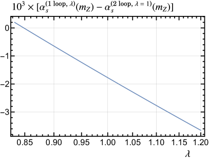
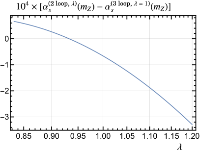
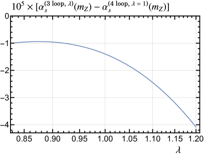
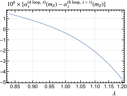
Figure 2: Values of $\alpha^{(5)}_{s}(m_{Z})$ over the $\beta$-function scaling parameter $\lambda$, obtained by evolving the strong coupling down from $\alpha^{(5)}_{s}(1508.04\,\mathrm{GeV})$ with different loop orders in the evolution equation. The value of $\alpha^{(5)}_{s}(m_{Z})$ computed by including one more perturbative order in the evolution with $\lambda=1$ is subtracted to highlight for which ranges of $\lambda$ both results for $\alpha^{(5)}_{s}(m_{Z})$ coincide or come close. The results indicate that a variation for $\lambda$ of about $10\%$ around $1$ is a reasonable range to estimate the perturbative uncertainty.

A different approach to estimate the perturbative error of $\alpha_{s}^{(5)}(m_{Z})$ is to vary the $\beta$-function scaling parameter $\lambda$ (controlled by the optional parameter lambdaAlpha) as described in Sec. 6.1.2. In Fig. 2 the value of $\alpha^{(5)}_{s}(m_{Z})$ is shown, obtained by evolving the strong coupling down from $\alpha^{(5)}_{s}(1508.04\,\mathrm{GeV})$ with different loop orders in the evolution equation and with varying values of $\lambda$; the value of $\alpha^{(5)}_{s}(m_{Z})$ obtained by including one more perturbative order in the evolution with $\lambda=1$ (which corresponds to the standard form of the $\beta$-function) is subtracted. We observe that, to reproduce a value near to the one obtained with one more perturbative order included in the running, $\lambda$ has to be varied by about $10\%$ around $1$, as already described in Sec. 6.1.2.

Assuming this to be also the appropriate range to estimate the perturbative uncertainty of the 5-loop result, the error can be estimated by scanning over $\lambda$ values. Employing REvolver for this task, we first define a list of $20$ logarithmically distributed values of $\lambda$ in the appropriate range

  In[]:= lamList = 1.1^Range[-1, 1, 2/19];

and create one Core for each value in $\lambda$. For convenience, the Core names are set to the associated $\lambda$ values

  In[]:= CoreCreate[ToString[#], {5, aQCentral, Q},
             lambdaAlpha -> #] & /@ lamList;

The span of values of $\alpha^{(5)}_{s}(m_{Z})$ corresponding to the range in $\lambda$ can then be obtained with

  In[]:= aLamList = AlphaQCD[ToString[#], mZdef] & /@ lamList;

The central value of this range and the associated error are consequently given by

  In[]:= (Max[aLamList] + {1, -1} * Min[aLamList])/2
  Out[]= {0.11624517272452983, 1.0224197660724244*^-7}

giving the same order of magnitude as the conservative approach. The variation in $\lambda$ of $\alpha^{(5)}_{s}(m_{Z})$ when employing 5-loop running is also depicted in Fig. 3.

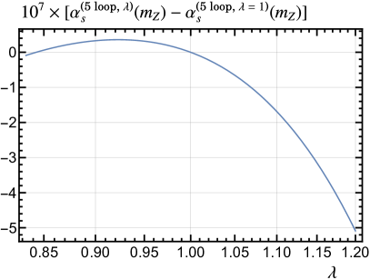
Figure 3: Variation of $\alpha^{(5)}_{s}(m_{Z})$ with $\lambda$, obtained by evolving the strong coupling down from $\alpha^{(5)}_{s}(1508.04\,\mathrm{GeV})$ with 5-loop accuracy. The value of $\alpha_{s}(m_{Z})$ for $\lambda=1$ is subtracted. Varying $\lambda$ in a range of about $10\%$ around $1$ the value of $\alpha_{s}(m_{Z})$ changes by $10^{-7}$.

7.1.2 Complex renormalization scales

In this application we illustrate the REvolver functionality to determine the strong coupling $\alpha_{s}(\mu)$ at complex scales $\mu$. To this end we consider the analyses in Refs. [25, 26], where the perturbative QCD corrections $\delta^{(0)}$ to the inclusive $\tau$ hadronic width were considered in fixed-order perturbation theory (FOPT) as well as contour-improved perturbation theory (CIPT). In the second reference a scheme different from the usual $\overline{\mathrm{MS}}$ definition is used for $\alpha_{s}$. We exploit this fact to demonstrate the ability of REvolver to deal with user-defined $\beta$-function coefficients.

Hadronic $\tau$ decay

In CIPT, determining $\delta^{(0)}$ involves integrating over powers of the strong coupling $\alpha_{s}^{(3)}(\mu)$ multiplied with a kinematic weight function in the complex $\mu^{2}$ plane along a circle with radius $m_{\tau}^{2}$

$$\delta^{(0)}_{\mathrm{CI}} =\sum_{n=1}^{\infty}c_{n,1}J_{n}^{a}(m_{\tau}^{2})\,,$$

$$J_{n}^{a}(m_{\tau}^{2}) =\frac{1}{2\pi i}\oint_{|x|=1}\!\frac{\mathrm{d}x}{x}(1-x)^{3}(1+x)\biggl{[}\frac{\alpha_{s}^{(3)}(\sqrt{-m_{\tau}\,x})}{\pi}\biggr{]}^{n}\,,$$ (7)

where the coefficients $c_{n,1}$ are given in Eqs. (2.13), (2.15) and (3.10) of Ref. [25]. In that article, 4-loop running for the strong coupling was used, as well as the input value $\alpha_{s}^{(3)}(m_{\tau})=0.34$. To reproduce the numbers for $\delta^{(0)}_{\mathrm{CI}}$ given in Eq. (3.9) of Ref. [25] we first define variables accounting for the employed input values

 In[]:= {nfa, aTau, mTau} = {3, 0.34, 1.77686};
        {c11, c21, c31, c41, c51} =
          {1, 1.640, 6.371, 49.076, 283};

and a function to compute $J_{n}^{a}(m_{\tau}^{2})$

  In[]:= Ja[n_, core_] := 1/(2 Pi)
            NIntegrate[(1 - E^(I phi))^3 (1 + E^(I phi))
              (AlphaQCD[core, Sqrt[-mTau^2 E^(I phi)]]/Pi)^n,
             {phi, 0, 2 Pi}];

where we change variables via $x=\exp(i\phi)$. Furthermore, we define a Core with 4-loop running for the coupling

  In[]:= CoreCreate["CI4", {nfa, aTau, mTau}, runAlpha -> 4]

All requirements are now set to reproduce the numbers given in Eq. (3.9) of Ref. [25]

  In[]:= Ja[1, "CI4"]*c11
         Ja[2, "CI4"]*c21
         Ja[3, "CI4"]*c31
         Ja[4, "CI4"]*c41
         Ja[5, "CI4"]*c51
  Out[]= 0.14789839179248082 + 0. I
  Out[]= 0.02968556861749222 - 1.3583618952083769*^-18 I
  Out[]= 0.0121854520515486 + 4.947098114161149*^-18 I
  Out[]= 0.008592183988059407 - 8.468364884304664*^-19 I
  Out[]= 0.0037863076541974016‘ - 9.919281576456942*^-19 I

with full agreement.

We can now easily inspect the corrections induced by the 5-loop running of the strong coupling by creating an appropriate Core

  In[]:= CoreCreate["CI5", {nfa, aTau, mTau}, runAlpha -> 5];

and evaluating

  In[]:= Ja[1, "CI5"]*c11
         Ja[2, "CI5"]*c21
         Ja[3, "CI5"]*c31
         Ja[4, "CI5"]*c41
         Ja[5, "CI5"]*c51
  Out[]= 0.14775354880331787 - 8.834874115176436*^-18 I
  Out[]= 0.02960219692750483 - 1.811149193611169*^-18 I
  Out[]= 0.012122455789576415 + 3.4080009230887917*^-18 I
  Out[]= 0.008521503950040327 - 1.6936729768609328*^-18 I
  Out[]= 0.0037376807938461127 - 1.5260433194549141*^-18 I

We observe a small negative $\mathcal{O}(1\%)$ shift in the individual coefficients. Note that the explicit specification of the running order runAlpha -> 5 at Core creation is not mandatory since 5-loop running is the default. We included it to be explicit.

Hadronic $\tau$ decay with $C$-scheme strong coupling

We now turn to Ref. [26] for which we reproduce the value quoted for $\delta^{(0)}_{\mathrm{CI}}$ in Eq. (22). To obtain this number the 3-flavor strong coupling, the related $\beta$-function coefficients and the coefficients $c_{n,1}$ were converted to a class of schemes for the strong coupling where the $\beta$-function adopts the following exact all order form

$$\hat{\beta}(\hat{\alpha}_{s})=-2\hat{\alpha}_{s}\frac{\frac{\hat{\alpha}_{s}}{4\pi}\beta_{0}}{1-\frac{\hat{\alpha}_{s}}{4\pi}\frac{\beta_{1}}{\beta_{0}}}\,=-2\hat{\alpha}_{s}\!\sum_{i=0}\hat{\beta}_{i}\biggl{(}\frac{\hat{\alpha}_{s}}{4\pi}\biggr{)}^{\!\!i+1}\,,$$ (8)

where $\hat{\beta}_{i}=\beta_{0}(\beta_{1}/\beta_{0})^{i}$. Within that class of schemes one needs to fix a parameter $C$ to uniquely specify the strong coupling. This parameter was set to $C=-1.246$ in Eq. (22) of Ref. [26] with the argument that the unknown 5-loop coefficient can then be neglected resulting in the value $\delta^{(0)}_{\mathrm{CI}}(\hat{\alpha}(m_{\tau}),C=-1.246)=0.1840\pm 0.0062$. The quoted uncertainty refers to the size of the 4-loop correction term. Solving Eq. (6) of the reference paper to convert the quoted value of the $\overline{\mathrm{MS}}$ strong coupling $\alpha_{s}^{(3)}(m_{\tau})=0.316$ to the scheme described above leads to $\hat{\alpha}_{s}(m_{\tau},C=-1.246)=0.477$. The transformed coefficients $c_{n,1}$ can be extracted from Eq. (12) therein. REvolver allows the order-by-order specification of user-defined $\beta$-functions, so we expand $\hat{\beta}(\hat{\alpha}_{s})$ up to $\mathcal{O}(\hat{\alpha}_{s}^{11})$.

We define the relevant input values related to $\hat{\alpha}_{s}$, the coefficients $c_{n,1}$ and $\hat{\beta}_{i}$ for $n_{f}=3$ with

  In[]:= {nfa, aTau, mTau} = {3, 0.477, 1.77686};
         {c11, c21, c31, c41} =
           {1, 1.640 + 2.25 c, 7.682 + 11.38 c + 5.063 c^2,
             61.06 + 72.08 c + 47.4 c^2 + 11.39 c^3} /.
            c -> -1.246;
         betaHat = 9. * (64/9)^Range[0, 9];

and the related Core

  In[]:= CoreCreate["Hat", {nfa, aTau, mTau}, betaHat]

Reusing the function Ja[n_, core_] as defined in the previous example we obtain

  In[]:= Ja[1, "Hat"]*c11 + Ja[2, "Hat"]*c21 +
          Ja[3, "Hat"]*c31 + Ja[4, "Hat"]*c41
  Out[]= 0.18403340012158337 - 1.0177988675705949*^-17 I

for $\delta^{(0)}_{\mathrm{CI}}(\hat{\alpha}(m_{\tau}),C=-1.246)$ and

  In[]:= Ja[4, "Hat"]*c41
  Out[]= 0.006222359703784199 - 2.951274747776552*^-19 I

for the last correction term. Both the central value and the size of the last correction term are in perfect agreement with Ref. [26].

Cauchy integral theorem for the strong coupling

It is worth mentioning that Cauchy’s integral formula can be utilized to check the numerical quality of the coupling evolution routine implemented in REvolver. For example, valuating $\alpha_{s}^{(3)}(2\,\mathrm{GeV})$ directly as well as by employing Cauchy’s integral formula with a radius of $1$ GeV gives equivalent results up to machine precision

  In[]:= mu0 = 2;
         aDirect = AlphaQCD["CI5", mu0]
         aResidue =
          1/(2 Pi) NIntegrate[AlphaQCD["CI5", mu0 + E^(I phi)],
            {phi, 0, 2 Pi}, PrecisionGoal -> 10]
         aResidue - aDirect
  Out[]= 0.3169005366613899
  Out[]= 0.31690053666139 + 1.1043592643970545*^-17 I
  Out[]= 1.1102230246251565*^-16 + 1.1043592643970545*^-17 I

For all practical purposes the solution for the strong coupling evolution provided by REvolver based on a given QCD $\beta$-function can be considered as exact.

7.2 Cores with one Massive Quark

In the previous sample applications the impact of flavor thresholds was not considered. In the following we discuss examples where threshold effects associated to one massive quark are accounted for.

7.2.1 Strong coupling with a flavor threshold

Strong coupling from multijet events

We consider Ref. [27], where the strong coupling value was determined by the ATLAS collaboration from transverse energy-energy correlations in multijet events based on $8$ TeV LHC data. The measurements were made for different values of the transverse momentum sum $H_{\mathrm{T2}}$ of the two leading jets. All values of $H_{\mathrm{T2}}$ considered in that analysis were much larger than the top quark mass, consequently the associated respective strong coupling values $\alpha_{s}^{(6)}(Q)$ are defined in the 6-flavor scheme. In Tabs. 2 and 3 of Ref. [27] values for $\alpha_{s}^{(6)}(Q)$ and the associated results for $\alpha_{s}^{(5)}(m_{Z})$ are quoted. For the strong coupling running an approximate analytic 2-loop solution of the evolution equation was used accounting for continuous matching at the top quark mass (which is correct for 1-loop matching when the matching scale is at the top quark mass). In the following, we focus on the associated results $\alpha_{s}^{(5)}(m_{Z})=0.1186^{+0.0090}_{-0.0047}$ and $\alpha_{s}^{(6)}(810\,\mathrm{GeV})=0.0907^{+0.0052}_{-0.0026}$, where for simplicity, we added the respective upper and lower uncertainties in quadrature. We reproduce the asymmetric uncertainties for $\alpha_{s}^{(6)}(810\,\mathrm{GeV})$ for the given $\alpha_{s}^{(5)}(m_{Z})$ range and start by defining the relevant parameters for the 5-flavor coupling $\alpha_{s}^{(5)}(m_{Z})$, where we set the top quark standard running mass to $\overline{m}_{t}=163$ GeV

  In[]:= {amZCentral, Q, mtmt} = {0.1186, 810, 163};
         {amZMax, amZMin} = amZCentral + {0.0090, -0.0047};

Next we create the Cores for our evaluation (including a CoreDeleteAll[] to remove older cores)

  In[]:= CoreDeleteAll[]
         CoreCreate["central2", 6, {5, amZCentral, mZdef},
          {{6, mtmt, mtmt}}, runAlpha -> 2]
         CoreCreate["max2", 6, {5, amZMax, mZdef},
          {{6, mtmt, mtmt}}, runAlpha -> 2]
         CoreCreate["min2", 6, {5, amZMin, mZdef},
          {{6, mtmt, mtmt}}, runAlpha -> 2]

To obtain the $6$-flavor strong coupling values at $Q=810$ GeV including the error range we simply evaluate

  In[]:= aQCentral2 = AlphaQCD["central2", Q, 6]
         AlphaQCD[#, Q, 6] & /@ {"min2", "max2"} - aQCentral2
  Out[]= 0.09079931707610696
  Out[]= {-0.002757013433150532, 0.005129916277931454}

agreeing very well with the result given in Ref. [27].

We investigate this setup with two-loop evolution further by determining the uncertainty related to varying the matching scale accounting for the top threshold corrections at one loop. This is easily done using REvolver by creating a set of Cores with a range of f-parameters. To this end we first define a table containing $20$ logarithmically scaled f-parameters in the range $[1/2,2]$, which corresponds to matching scales between one half and twice the standard running top mass. Subsequently the table is used to create the corresponding set of Cores

  In[]:= list2 = 2^Range[-1, 1, 2/19];
  In[]:= CoreCreate[ToString[#] <> "run2", 6,
             {5, amZCentral, mZdef}, {{6, mtmt, mtmt}},
             runAlpha -> 2, orderAlpha -> 1,
             fMatch -> {#}] & /@ list2;

Finally, we can determine a list of the corresponding strong coupling values $\alpha_{s}^{(6)}(810\,\mathrm{GeV})$ and compute the central value as well as the error range

  In[]:= aQList2 = AlphaQCD[ToString[#] <> "run2", Q, 6] & /@
            list2;
         (Max[aQList2] + {1, -1} * Min[aQList2])/2
  Out[]= {0.09081555469961156, 0.00009936201139525841}

The perturbative uncertainties associated to the threshold corrections are about $3\%$ of the quoted experimental error.

Employing 5-loop instead of 2-loop running for the strong coupling and 4-loop matching corrections we obtain

  In[]:= CoreCreate["central5", 6, {5, amZCentral, mZdef},
          {{6, mtmt, mtmt}}, runAlpha -> 5]
         CoreCreate["max5", 6, {5, amZMax, mZdef},
          {{6, mtmt, mtmt}}, runAlpha -> 5]
         CoreCreate["min5", 6, {5, amZMin, mZdef},
          {{6, mtmt, mtmt}}, runAlpha -> 5]
  In[]:= aQCentral5 = AlphaQCD["central5", Q, 6]
         AlphaQCD[#, Q, 6] & /@ {"min5", "max5"} - aQCentral5
  Out[]= 0.09078701609518454
  Out[]= {-0.00275523573924355, 0.0051259314534172346}

for $\alpha_{s}^{(6)}(810\,\mathrm{GeV})$ and its upper and lower uncertainty and

  In[]:= CoreCreate[ToString[#] <> "run5", 6,
             {5, amZCentral, mZdef}, {{6, mtmt, mtmt}},
             runAlpha -> 5, fMatch -> {#}] & /@ list2;
  In[]:= aQList5 = AlphaQCD[ToString[#] <> "run5", Q, 6] & /@
            list2;
         (Max[aQList5] + {1, -1} * Min[aQList5])/2
  Out[]= {0.09078682756270738, 1.9445996186917558*^-7}

for the central value and error estimate derived from varying the matching scale. Within the experimental uncertainties as quoted in Ref. [27] using 2-loop evolution and continuous matching is perfectly adequate.

Strong coupling from inclusive jet cross sections

We return to the analysis of Ref. [24] and investigate the impact of a top quark threshold on the values given there, staying with 2-loop running as employed in that reference. In the following we create Cores with the given range of values of $\alpha_{s}^{(5)}(m_{Z})=0.1162^{+0.0070}_{-0.0062}$ and determine the strong coupling $\alpha_{s}^{(6)}(1508.04\,\mathrm{GeV})$ in the 6-flavor scheme instead of the 5-flavor coupling $\alpha_{s}^{(5)}(1508.04\,\mathrm{GeV})$ determined in Ref. [24]. After defining the parameters

  In[]:= {amZCentral, Q, mtmt} = {0.1162, 1508.04, 163};
         {amZMax, amZMin} = amZCentral + {0.007, -0.0062};

and creating the respective Cores, accounting for the standard running top quark mass $\overline{m}_{t}=163$ GeV and default 4-loop matching

  In[]:= CoreCreate["central2", 6, {5, amZCentral, mZdef},
           {{6, mtmt, mtmt}}, runAlpha -> 2];
         CoreCreate["min2", 6, {5, amZMin, mZdef},
           {{6, mtmt, mtmt}}, runAlpha -> 2];
         CoreCreate["max2", 6, {5, amZMax, mZdef},
           {{6, mtmt, mtmt}}, runAlpha -> 2];

we obtain

  In[]:= aQCentral2 = AlphaQCD["central2", Q, 6]
         (AlphaQCD[#, Q, 6] & /@ {"min2","max2"}) - aQCentral2
  Out[]= 0.08406136347372324
  Out[]= {-0.003262229612787812, 0.0035626775539831235}

for the central value and the upper and lower uncertainties, respectively. Comparing these values to $\alpha_{s}^{(5)}(1508.04\,\mathrm{GeV})=0.0822^{+0.0034}_{-0.0031}$, quoted in Ref. [24], we observe a positive shift of about $0.002$ in the central value. This already amounts to about $60\%$ of the given experimental error, illustrating that flavor-thresholds effects can lead to significant changes.

7.2.2 Asymptotic pole and low-scale MSR mass

To demonstrate the REvolver functionalities related to mass conversions accounting for flavor threshold effects, we investigate how much the asymptotic top quark pole mass $m_{t}^{\rm pole}$ as well as the top MSR mass at $2$ GeV $m_{t}^{\rm MSR}(2\,\mbox{GeV})$ would change if the strong coupling value quoted in Ref. [24] $\alpha_{s}(1508.04\,\mbox{GeV})=0.0822^{+0.0034}_{-0.0031}$ would be interpreted as a $6$-flavor compared to a $5$-flavor result. After defining the relevant constants and Cores (we keep using the values of Q and mtmt already defined in the previous section)

  In[]:= aQ = 0.0822;
         CoreCreate["5", 6, {5, aQ, Q}, {{6, mtmt, mtmt}}];
         CoreCreate["6", 6, {6, aQ, Q}, {{6, mtmt, mtmt}}];

where we have employed default highest-order precision for coupling and mass evolution and flavor threshold matching, we first extract $m_{t}^{\mathrm{MSR}}(2\,\mathrm{GeV})$ from both Cores and then determine their difference:

  In[]:= mMSR25 = MassMS["5", 6, 2]
         mMSR26 = MassMS["6", 6, 2]
         mMSR25 - mMSR26
  Out[]= 172.45858180514585
  Out[]= 172.10074770514723
  Out[]= 0.3578340999986267

For the asymptotic pole masses we obtain

  In[]:= mPole5 = MassPole["5", 6, mtmt]
         mPole6 = MassPole["6", 6, mtmt]
         mPole5 - mPole6
  Out[]= 172.8732843267365
  Out[]= 172.4868549739421
  Out[]= 0.3864293527944085

where we adopted $\overline{m}_{t}=163$ GeV as the conversion scale for the asymptotic pole mass determination. The differences we obtain amount to $358$ MeV and $386$ MeV, both of which exceed the uncertainty of the current world average for direct top mass measurements [23].

7.2.3 Bottom and charm quark short-distance masses

Bottom $\overline{\mathrm{MS}}$ mass at high scales

In Ref. [28] the partonic cross section for Higgs production via bottom quark fusion was presented. This involves the bottom running mass at the Higgs scale $m_{H}=125.09$ GeV, quoted to be $m_{b}^{(5)}(m_{H})\equiv\overline{m}_{b}^{(5)}(m_{H})=2.79$ GeV using 4-loop $\overline{\mathrm{MS}}$-mass running, $\alpha_{s}^{(5)}(m_{Z})=0.118$ and the bottom quark standard running mass $\overline{m}_{b}=4.18$ GeV, see Table 2 therein. We can reproduce this relation in REvolver by defining the relevant parameters

  In[]:= {mH, amZ, mbmb} = {125.09, 0.118, 4.18};

and creating a corresponding Core

  In[]:= CoreDeleteAll[]
         CoreCreate["b", 5, {5, amZ, mZdef}, {5, mbmb, mbmb},
            runMSbar -> 4]

The value of $m_{b}^{(5)}(m_{H})$ can now be extracted with

  In[]:= MassMS["b", 5, mH]
  Out[]= 2.78854676339097

showing perfect agreement with Ref. [28].

Bottom quark PS and 1S masses

In Ref. [29] the conversion between the $\overline{\mathrm{MS}}$ and various low-scale short-distance masses was carried out with 4-loop fixed-order formulae. To illustrate the functionalities of REvolver for mass conversions we now consider the values of the PS and 1S bottom quark masses given in Table II of that article. We start defining the input parameters $\alpha_{s}^{(5)}(m_{Z})=0.1185$, $\overline{m}_{b}=4.163$ GeV and $\mu_{f}=2.0$ GeV for the strong coupling, the standard running bottom mass and the bottom PS mass renormalization scale, respectively, as specified in Ref. [29],

  In[]:= {amZ, mbmb, mufB} = {0.1185, 4.163, 2.0};

and the related Core

  In[]:= CoreCreate["b", 5, {5, amZ, mZdef},
          {{5, mbmb, mbmb}}, fMatch -> {2.0}]

Following Ref. [29] we set the bottom quark matching scale to twice the standard running bottom mass. Comparing the 4-loop value for the bottom PS mass $m_{b}^{\rm PS}(2\,\mbox{GeV})=4.483$ GeV quoted in Ref. [29] and obtained by REvolver we obtain

  In[]:= mbPSRef = 4.483;
         mbPSREvo = MassPS["b", 5, mufB, 5, mbmb, mbmb]
         mbPSREvo - mbPSRef
  Out[]= 4.484037803646092
  Out[]= 0.0010378036460920725

where, following Ref. [29], the conversion is carried out using the fixed-order relation between the standard running and PS masses using the standard running mass $\overline{m}_{b}$ as the renormalization scale for the strong coupling.

The small difference of about $1$ MeV results from the fact that in REvolver all conversions between mass schemes are based on formulae starting from the value of the running mass, while in Ref. [29] the conversion was obtained the other way around, i.e. the running mass was computed starting from a value in the PS scheme. The difference is naturally covered by the perturbative uncertainty and not relevant for practical purposes.

In the previous example we have used REvolver to determine the PS from the standard running mass $\overline{m}_{b}$. The conversion in the opposite direction can be achieved using the REvolver functionality to add a heavier mass to an existing Core, see Sec. 6.3. To determine the standard running mass we first create a Core containing $4$ massless flavors

  In[]:= anf4mu3 = AlphaQCD["b", 3.0, 4];
         CoreCreate["O4", {4, anf4mu3, 3.0}]

which requires the 4-flavor strong coupling $\alpha_{s}^{(4)}(3\,\mathrm{GeV})$ as an input, which here we obtain from the previously created Core named b.

We now create a new Core with name b2 by adding the bottom PS mass $m_{b}^{\rm PS}(2\,\mbox{GeV})=4.483$ GeV to the Core named O4, reusing the parameters mbPSRef and mufB defined in the previous example as well as the matching scale factor $2.0$, specified by the option parameter fnQ

  In[]:= AddPSMass["O4", "b2", mbPSRef, mufB, 5, 4.2,
          4.2, fnQ -> 2.0]

Internally, first the 5-flavor running mass is determined and subsequently used to create the 5-flavor Core named b2. To match precisely the conversion method used in Ref. [29] we set the running mass scale and the renormalization scale of the strong coupling for that conversion to $4.2$ GeV here.

Reading out the resulting bottom quark standard running mass results in

  In[]:= MassMS["b2", 5]
  Out[]= 4.1621220500397325

with the expected $1$ MeV difference to the value $\overline{m}_{b}=4.163$ GeV quoted in the reference paper. This difference arises here again because the numerical conversion formulae employed in REvolver are exactly invertible, i.e. they produce the same numerical mass differences regardless in which way the conversion is carried out.

Note that the default REvolver routines convert from the MSR mass to a low-scale short-distance mass at the intrinsic scale of the low-scale short-distance mass (see Sec. 6.2.2) to resum potentially large logarithms involving the ratio of the quark mass and the renormalization scale. In the example above, we have, however, explicitly set the input parameter nfConv of the function MassPS to $5$ to enforce conversion at the scale of the $\overline{\mathrm{MS}}$ mass (which is the approach used in Ref. [29] and which does not resum these logarithms). The result including log-resummation via R-evolution differs by around $15$ MeV and can be extracted by using the corresponding REvolver commands with default parameter settings. For example, converting from the standard running mass to the PS mass we obtain

  In[]:= MassPS["b", 5, mufB]
  Out[]= 4.468247788253957

where nfConv is automatically set to $4$ and $R$ as well as the renormalization scale of the strong coupling are set to mufB.

The corresponding (log-resummed) conversion from the PS mass to the standard running mass is achieved by adding to the Core named O4 the bottom quark PS mass $m_{b}^{\rm PS}(2\,\mbox{GeV})=4.483$ GeV, specifying log resummation via R-evolution. The associated new Core named b3 is created by

  In[]:= AddPSMass["O4", "b3", mbPSRef, mufB, fnQ -> 2.0]

resulting in a bottom quark standard running mass of

  In[]:= MassMS["b3", 5]
  Out[]= 4.176206116625182

At this point it should be mentioned that for bottom quarks large scale hierarchies cannot arise, such that the log-resummed conversion is not superior and the difference between the fixed-order and the log-resummed conversions may be better considered as a scheme variation. To illustrate this we show, order by order, the bottom quark PS mass computed in the fixed-order expansion as well as by utilizing R-evolution:

  In[]:= MassPS["b", 5, mufB, 5, mbmb, mbmb, 1.0, #] & /@
          {1, 2, 3, 4}
         MassPS["b", 5, mufB, 4, mufB, mufB, 1.0, #] & /@
          {1, 2, 3, 4}
  Out[]= {4.371486051575019, 4.452182487749768,
          4.484416838176134, 4.484037803646092}
  Out[]= {4.456398324160689, 4.487678320598545,
          4.494296775616467, 4.468247788253957}

Next, we consider the 1S scheme. Comparing the 1S bottom quark mass $m_{b}^{\rm 1S}=4.670$ GeV quoted Ref. [29] and obtained in REvolver using the relativistic counting and conversion at the high scale $\overline{m}_{b}$ (which again agrees with the approach used in Ref. [29] and does not account for the resummation of logarithms involving the bottom mass and inverse Bohr radius) we obtain

  In[]:= mb1SRef = 4.670;
         mb1SRevo = Mass1S["b", 5, 5, mbmb, "relativistic"]
         mb1SRevo - mb1SRef
  Out[]= 4.671281708897272
  Out[]= 0.0012817088972720825

Again, the $1$ MeV discrepancy emerges from the perturbative difference between converting from or to the standard running mass. For comparison, we also present the corresponding 1S mass value accounting for log-resummation via R-evolution. This can be achieved by calling the routine Mass1S without any optional parameters. This implies that the default setting is used, namely that the 1S mass is converted from the MSR mass at the inverse Bohr radius $M_{q,B}$ (the intrinsic scale of the 1S mass, see Sec. 6.2.2) and that non-relativistic counting is applied. The bottom 1S mass is, however, sensitive to the ultra-soft scale $M^{2}_{q,B}/m_{b}$, related to logarithms of the strong coupling. This entails that for the conversion from the MSR mass (at the inverse Bohr radius) a scale larger than $M_{q,B}$ may be adopted as the renormalization scale for the strong coupling to avoid perturbative instabilities. Adopting $2M_{q,B}$ for the renormalization scale of the strong coupling, the 1S mass accounting for log-resummation is obtained by

  In[]:= MbB = MBohr["b", 5]
         Mass1S["b", 5, 4, MbB, "nonrelativistic", 2*MbB]
  Out[]= 1.8792648142678285
  Out[]= 4.6676688462595175

The result differs by $4$ MeV to the one using fixed-order conversion. As for the bottom PS mass, there is no conceptual improvement using log-resummation. This can again be seen from comparing the 1S mass values at lower orders. Order by order, the values of the bottom quark 1S mass, derived in fixed-order and with R-evolution, respectively, are given by

  In[]:= Mass1S["b", 5, 5, mbmb, "relativistic", mbmb, #] & /@
          {1, 2, 3, 4}
         Mass1S["b", 5, 4, MbB, "nonrelativistic", 2*MbB,
          #] & /@ {1, 2, 3, 4}
  Out[]= {4.516545706062886, 4.64055194539697,
          4.680062686477036, 4.671281708897272}
  Out[]= {4.609340303152403, 4.666301702298438,
          4.6809114692112495, 4.6676688462595175}

Of course one can also convert from the 1S scheme to the standard running mass using the routine Add1SMass, shortly demonstrated in the following.

Reusing the Core named O4, which contains $4$ massless quarks, we create a new Core with name b4 by adding the bottom 1S mass using fixed-order conversion

  In[]:= Add1SMass["O4", "b4", mb1SRef, 5, mbmb,
          "relativistic", mbmb, fnQ -> 2.0]

which results in the following bottom quark standard running mass:

  In[]:= MassMS["b4", 5]
  Out[]= 4.161807379452769

again with the expected $1$ MeV difference to the value $\overline{m}_{b}=4.163$ GeV quoted in Ref. [29], related to invertible numerical conversion algorithm employed in REvolver. The analogous procedure for converting the 1S mass to the standard running mass using R-evolution can be performed by executing

  In[]:= Add1SMass["O4", "b5", mb1SRef, 4, MbB,
          "nonrelativistic", 2*MbB, fnQ -> 2.0]
  In[]:= MassMS["b5", 5]
  Out[]= 4.165169213761735

Charm and bottom quark RS masses

In Ref. [30] the charm quark RS mass $m_{c}^{\rm RS}(\nu_{f})=1.202$ GeV at the scale $\nu_{f}=1$ GeV was extracted from charmonium bound states masses, given in Eq. (2.15) of that paper. The RS mass was converted to the standard running charm mass $\overline{m}_{c}=1.217$ GeV with 4-loop fixed-order formulae for $\alpha_{s}^{(5)}(m_{Z})=0.1184$ and using $\mu_{c}=1.27$ GeV as the charm threshold matching scale. The renormalization scale of the strong coupling was set to $\nu_{c}=1.5$ GeV and the pole mass renormalon normalization constant for $n_{f}=3$ active flavors was quoted to be $N_{m}=0.5626$. This relation can be easily reproduced with REvolver. First, we set the relevant variables

  In[]:= {amZ, Nm} = {0.1184, 0.5626};
         {mcmc, mcmcMatch, nufc, nuc} =
          {1.217, 1.27, 1.0, 1.5};
         {mbmb, mbmbMatch} = {4.185, 4.2};

and create the respective Core

  In[]:= CoreDeleteAll[]
         CoreCreate["cb", 5, {5, amZ, mZdef},
          {{4, mcmc, mcmc}, {5, mbmb, mbmb}},
          fMatch -> {mcmcMatch/mcmc, mbmbMatch/mbmb}]

We include the standard running bottom mass $\overline{m}_{b}=4.185$ GeV with the corresponding threshold matching scale $\mu_{b}=4.2$ GeV to enable automatic matching of the strong coupling constant which is given at $\mu=m_{Z}$. The charm quark RS mass computed by REvolver and the difference to the value quoted in the reference paper are given by

  In[]:= mcRSRef = 1.202;
         mcRSREvo = MassRS["cb", 4, nufc, 4, mcmc, nuc,
           4, 4, Nm]
         mcRSRef - mcRSREvo
  Out[]= 1.201144351209422
  Out[]= 0.0008556487905779786

showing agreement at the sub-MeV level.

In Ref. [30] also the bottom quark RS mass value $m_{b}^{\rm RS}(\nu_{f})=4.379$ GeV at the scale $\nu_{f}=2$ GeV was extracted from bottomonium meson masses [ see Eq. (2.3) of that paper ] and subsequently converted to the standard running bottom mass $\overline{m}_{b}=4.379$ GeV with 4-loop fixed-order formulae using $\mu_{b}=4.2$ GeV as the bottom threshold matching scale and $\nu_{b}=2.5$ GeV as the renormalization scale of the strong coupling. The charm mass corrections in the perturbative relation between the RS and the $\overline{\mathrm{MS}}$ mass have been implemented in an effective way by evaluating the conversion series that relates the $\overline{\mathrm{MS}}$ and the RS masses for the bottom quark and $n_{\ell}$ massless quarks for $n_{\ell}=3$ dynamical flavors, but using the 3-flavor strong coupling $\alpha_{s}^{(3)}$ computed with the charm mass threshold properly accounted for. This treats the charm quark as a decoupled flavor. The REvolver RS mass routines do not directly provide this functionality, but in the following we show how this evaluation can still be carried out in REvolver. We first set the necessary parameters not yet defined before

  In[]:= {nufb, nub} = {2.0, 2.5};

and compute the 3-flavor strong coupling $\alpha_{s}^{(3)}(\mu_{c})$ at the charm matching scale $\mu_{c}=1.27$ GeV, taking into account the bottom as well as charm quark thresholds in the usual way

  In[]:= as3 = AlphaQCD["cb", mcmcMatch, 3];

Next, we define a Core with decoupled charm quarks by using the precomputed $n_{f}=3$ strong coupling and specifying a total number of $4$ flavors, including $3$ massless flavors and the massive bottom quark as the 4-th flavor

  In[]:= CoreCreate["b", 4, {3, as3, mcmcMatch},
          {4, mbmb, mbmb}, fMatch -> {mbmbMatch/mbmb}]

Setting all previously defined scales we get

  In[]:= mbRSRef = 4.379;
         mbRSREvo = MassRS["b", 4, nufb, 4, mbmb, nub,
           4, 4, Nm]
         mbRSREvo - mbRSRef
  Out[]= 4.379013026999629
  Out[]= 0.00001302699962923981

for the bottom quark mass in the RS scheme with a negligible difference to the value quoted in the reference article.

We can also convert from the bottom RS to the standard running mass using the REvolver routine AddRSMass. To do that, we first create a Core containing the $3$ massless non-decoupled flavors with

  In[]:= CoreCreate["O3", {3, as3, mcmcMatch}]

and subsequently create a new Core with name b2 by adding the bottom RS mass to the Core with name O3 setting the various input parameters in analogy to the example above, i.e. using fixed-order conversion

  In[]:= AddRSMass["O3", "b2", mbRSRef, nufb, 4, 4.2, nub, 4,
          4, Nm]

Internally, first the 5-flavor running mass is determined and subsequently used to create the Core named b2. We set the running mass scale for that conversion to $4.2$ GeV.

Extracting the bottom quark standard running mass from the newly created Core results in

  In[]:= MassMS["b2", 4]
  Out[]= 4.184987620121892

Bottom quark kinetic masses

In Ref. [21] the 3-loop corrections to the perturbative relation between the pole and kinetic quark mass schemes have been determined for the case of one massive quark and $n_{\ell}$ massless quarks. Here we show how to employ REvolver to reproduce the values for the bottom quark kinetic mass $m_{b}^{\rm kin}(\mu)$ at the scale $\mu=1$ GeV given in Eq. (8) of that paper, obtained by converting from the standard running mass $\overline{m}_{b}=4.163$ GeV.

The conversion from $\overline{m}_{b}$ to the bottom kinetic mass was considered using the perturbative series computed with the massive bottom quark and $n_{\ell}$ massless quarks for $n_{\ell}=4$ (i.e. with the charm quark treated as massless) with the result $m_{b}^{\rm kin}(\mu)=4.523$ GeV, as well as for $n_{\ell}=3$ (i.e. with the charm quark treated as decoupled) with the result $m_{b}^{\rm kin}(\mu)=4.521$ GeV. The first case can be reproduced in a straightforward way with REvolver as it corresponds to a realistic physical scenario.

First we define the relevant parameters

  In[]:= {mbmb, amZ, muCutb} = {4.163, 0.1179, 1.0};

and create a Core in which the charm quark is treated as massless

  In[]:= CoreDeleteAll[];
         CoreCreate["b4", 5, {5, amZ, mZdef},
          {{5, mbmb, mbmb}}]

The value obtained by REvolver and the difference to the value quoted in Ref. [21] is

  In[]:= mKinb4Ref = 4.523;
         mKinb4REvo = MassKin["b4", 5, muCutb, 5, mbmb, mbmb]
         mKinb4REvo - mKinb4Ref
  Out[]= 4.523457226246508
  Out[]= 0.0004572262465085686

i.e. there is perfect agreement.

The second case is in close analogy to the treatment of the RS mass just discussed above and requires that the conversion series, which relates the $\overline{\mathrm{MS}}$ and the kinetic mass for the bottom quark and $n_{\ell}$ massless quarks, is evaluated for $n_{\ell}=3$ dynamical flavors, but using the 3-flavor strong coupling $\alpha_{s}^{(3)}$ computed with the charm mass threshold properly accounted for. REvolver does not provide functionality to carry out this conversion directly, but in the following we show how this evaluation can still be performed.

To obtain the $n_{f}=3$ strong coupling in the usual way, we first create a new Core involving a massive bottom as well as charm quark

  In[]:= mcmc = 1.263;
         CoreCreate["bc", 5, {5, amZ, mZdef},
          {{4, mcmc, mcmc}, {5, mbmb, mbmb}}]

and extract $\alpha_{s}^{(3)}(\overline{m}_{b})$

  In[]:= a3mbmb = AlphaQCD["bc", mbmb, 3];

Next, we create the Core to be employed for the mass scheme conversion. We use the computed $n_{f}=3$ strong coupling and specify a total number of $4$ flavors with $3$ massless flavors and the massive bottom quark

  In[]:= CoreCreate["b3", 4, {3, a3mbmb, mbmb},
          {{4, mbmb, mbmb}}]

The value of the kinetic bottom quark mass computed by REvolver and the difference to the corresponding result quoted in Ref. [21] can now be obtained by

  In[]:= mKinb3Ref = 4.521;
         mKinb3REvo = MassKin["b3", 4, muCutb, 4, mbmb, mbmb]
         mKinb3Ref - mKinb3REvo
  Out[]= 4.520784332346221
  Out[]= 0.00021566765377922792

The numbers are in perfect agreement.

In Ref. [22] the lighter flavor mass corrections to the relation between the pole and kinetic masses were computed explicitly up to ${\cal O}(\alpha_{s}^{3})$. These corrections are implemented in REvolver. They have the property that they exclusively come from the flavor number decoupling relations of the strong coupling, and they are also referred to as “scheme B” in that reference. In Eq. (79) of that reference the bottom quark kinetic mass $m_{b}^{\mathrm{kin}}(1\,\mathrm{GeV})=4.526$ GeV was obtained using $\alpha_{s}^{(5)}(m_{Z})=0.1179$ for the strong coupling, the charm quark running mass $\overline{m}_{c}(2\,\mathrm{GeV})=0.993$ GeV and the bottom quark standard running mass $\overline{m}_{b}=4.136$ GeV. For the calculation, fixed-order conversion was applied using the standard running bottom mass $\overline{m}_{b}$ as the renormalization scale of the strong coupling. To reproduce the result with REvolver we define the input values with

  In[]:= {amZ, mc3, mbmb} = {0.1179, 0.993, 4.163};

and the related Core with

  In[]:= CoreDelete["bc"]
         CoreCreate["bc", 5, {5, amZ, mZdef},
           {{4, mc3, 3}, {5, mbmb, mbmb}}]

The bottom quark kinetic mass extracted by REvolver and its difference to the reference value are returned by

  In[]:= mbKinRef = 4.526;
         mbKinREvo = MassKin["bc", 5, 1.0, 5, mbmb, mbmb]
         mbKinRef - mbKinREvo
  Out[]= 4.527084826155039
  Out[]= -0.0010848261550391314

The small deviation of $1$ MeV originates from the fact that in Ref. [22] the light massive flavor corrections related to the charm quark are parametrized in terms of $\overline{m}_{c}(3\,\mathrm{GeV})$, while in REvolver they are parametrized in terms of the charm standard running mass $\overline{m}_{c}$.

Performing the same conversion with R-evolution to resum logarithms of the intrinsic physical scales of the mass schemes gives

  In[]:= MassKin["bc", 5, 1.0]
  Out[]= 4.53472077059131

i.e. the bottom quark kinetic mass with log-resummation is larger by about $7$ MeV. We note that, following Ref. [22], the default value for the kinetic mass intrinsic scale (where the default log-resummed conversion between the running and the kinetic mass is carried out) is set to be twice its renormalization scale, that is, $2$ GeV in the example above.

7.2.4 Top quark mass at low scales

We return to Ref. [29] and investigate the top quark mass conversion between the $\overline{\mathrm{MS}}$ and various short-distance schemes with 4-loop accuracy. This concerns Table I of that article.

Following Ref. [29] we first define the values for the strong QCD coupling $\alpha_{s}^{(5)}(m_{Z})=0.1185$, the top quark standard running mass $\overline{m}_{t}=163.643$ GeV and the renormalization scale of the PS mass $\mu_{f}=20$ GeV

  In[]:= {amZ, mtmt, mufT} = {0.1185, 163.643, 20.0};

and a Core with a top threshold matching scale of twice the top standard running mass

  In[]:= CoreDeleteAll[]
         CoreCreate["t", 6, {5, amZ, mZdef}, {{6, mtmt, mtmt}},
          fMatch -> {2.0}]

In analogy to Sec. 7.2.3, we evaluate the PS and 1S top quark mass employing REvolver and determine the difference to the values $m_{t}^{\rm 1S}=172.227$ GeV and $m_{t}^{\rm PS}(20\,\mbox{GeV})=171.792$ GeV quoted in the reference paper by converting directly from the $\overline{\mathrm{MS}}$ scheme, leading to

  In[]:= mtPSRef = 171.792;
         mtPSRevo = MassPS["t", 6, mufT, 6, mtmt, mtmt]
         mtPSRevo - mtPSRef
  Out[]= 171.7950829141975
  Out[]= 0.0030829141975061702

for the PS scheme, and

  In[]:= mt1SRef = 172.227;
         mt1SRevo = Mass1S["t", 6, 6, mtmt, "relativistic"]
         mt1SRevo - mt1SRef
  Out[]= 172.2298841816133
  Out[]= 0.0028841816132967324

for the 1S scheme, respectively.

As already described in Sec. 7.2.3, the small difference (of about $3$ MeV) results from the fact that in REvolver conversion is based on formulae where the (standard) running mass is taken as the input, while in Ref. [29] the conversion was carried out starting from the PS and 1S masses.

We now investigate the influence of large logarithms of the ratio between the top quark mass and the intrinsic scale of the respective short-distance schemes. For the top quark the impact of the summation of these logarithms can be significant. To this end we consider the convergence of the perturbative series relating the standard running top mass $\overline{m}_{t}$ to the PS mass $m_{t}^{\rm PS}(20\,\mbox{GeV})$, the 1S mass $m_{t}^{\rm 1S}$ as well as the running mass $m_{t}^{(5)}(2\,\mathrm{GeV})$.

Using fixed-order conversion (without log-resummation) from $\overline{m}_{t}$ and using $\overline{m}_{t}$ as the renormalization scale, the top PS mass at $4$ loops, and the corresponding corrections of order $\mathcal{O}(\alpha_{s}^{n})$ with $1\leq n\leq 4$ amount to

  In[]:= MassPS["t", 6, mufT, 6, mtmt, mtmt]
         Table[
          MassPS["t", 6, mufT, 6, mtmt, mtmt, 1.0, n] -
           MassPS["t", 6, mufT, 6, mtmt, mtmt, 1.0, n - 1],
          {n, 1, 4}]
  Out[]= 171.7950829141975
  Out[]= {6.636196514422409, 1.199280138792858,
          0.26779429813998945, 0.048811962842222556}

On the other hand, employing R-evolution to first evolve down to the PS mass renormalization scale $\mu_{f}=20$ GeV and then converting to the PS mass at that scale, which is REvolvers default procedure, we obtain

  In[]:= MassPS["t", 6, mufT]
         Table[
          MassPS["t", 6, mufT, 5, mufT, mufT, 1.0, n] -
           MassPS["t", 6, mufT, 5, mufT, mufT, 1.0, n - 1],
          {n, 1, 4}]
  Out[]= 171.79912206134247
  Out[]= {0., 0.06895809427228983,
          0.001838267705210228, -0.01976315025407871}

We observe that the corrections are considerably smaller when R-evolution is accounted for and that there is a difference of around $4$ MeV in the final 4-loop converted values for the two approaches. The $\mathcal{O}(\alpha_{s})$ correction term is zero in the case of the log-resummed conversion since the 1-loop perturbative coefficients of the PS and MSR masses coincide.

For the conversion to the 1S mass the observation regarding fixed-order versus log-resummed conversion is similar. In the fixed-order case we get

  In[]:= Mass1S["t", 6, 6, mtmt, "relativistic", mtmt]
         Table[
          Mass1S["t", 6, 6, mtmt, "relativistic", mtmt, n] -
           Mass1S["t", 6, 6, mtmt, "relativistic",
            mtmt, n - 1], {n, 1, 4}]
  Out[]= 172.2298841816133
  Out[]= {7.129280949172028, 1.227243021981991,
          0.21914263057425387, 0.01121757988499894}

while the log-resummed evaluation gives again substantially smaller corrections:

  In[]:= mBohr = MBohr["t", 6]
         Mass1S["t", 6, 5]
         Table[
          Mass1S["t", 6, 5, mBohr, "nonrelativistic",
            mBohr, n] - Mass1S["t", 6, 5, mBohr,
            "nonrelativistic", mBohr, n - 1], {n, 1, 4}]
  Out[]= 32.11684612826197
  Out[]= 172.20797480544945
  Out[]= {1.1666583987086199, 0.18536848855083576,
          -0.047109547951663444, -0.010351024770614004}

where the inverse Bohr radius, i.e. the intrinsic scale of the 1S mass, is shown as the first output for completeness.

Finally, we investigate the effect of log-resummation on the computation of the top quark $5$-flavor running mass at $2$ GeV, $m_{t}^{(5)}(2\,\mathrm{GeV})$, when converting from $m_{t}^{(5)}(\overline{m}_{t})$. For simplicity we create a new Core named t, this time where for the top threshold matching scale the default value, the top quark standard running mass, is adopted:

  In[]:= CoreDelete["t"]
         CoreCreate["t", 6, {5, amZ, mZdef},
           {{6, mtmt, mtmt}}];

Now we extract the value of the 5-flavor MSR mass $m_{t}^{(5)}(\overline{m}_{t})$ at the scale of the standard top running mass from this Core as a reference

  In[]:= m5mt = MassMS["t", 6, mtmt, 5]
  Out[]= 163.67571467667918

REvolver does not provide fixed-order conversions of the running masses between two different renormalization scales. It is, however, possible to access these fixed-order corrections through the pole mass routine MassPoleFO. Care has to be taken that the two calls of the MassPoleFO routines involve the same renormalization scale (which here is the standard running mass) to ensure that the pole mass renormalon is properly canceled:

  In[]:= FOTab =
           MassMS["t", 6, 2.0, 5] -
              MassPoleFO["t", 6, 5, 2.0, mtmt, #] +
              MassPoleFO["t", 6, 5, mtmt, mtmt, #] & /@
            {0, 1, 2, 3, 4};
         FOTab[[5]]
         Table[FOTab[[n]] - FOTab[[n - 1]], {n, 2, 5}]
  Out[]= 173.2337130005733
  Out[]= {7.46778271952536, 1.5242807051151317,
          0.4246371655552821, 0.14129773369833742}

The difference of the two calls of the MassPoleFO routine removes the log-resummed corrections from the output of MassMS and replaces it by the corresponding fixed-order terms. As for the above examples, we first display the $m_{t}^{(5)}(2\,\mathrm{GeV})$ value at $\mathcal{O}(\alpha_{s}^{4})$ and the fixed-order perturbative correction terms at order $\mathcal{O}(\alpha_{s}^{n})$ with $1\leq n\leq 4$.

For the investigation of the correction terms in the case of R-evolution we create four Cores, setting the respective loop order $n$ of the R-evolution equation to $1\leq n\leq 4$

  In[]:= CoreCreate["t-R" <> ToString[#], 6, {5, amZ, mZdef},
             {{6, mtmt, mtmt}}, runMSR -> #] & /@ {1, 2, 3, 4};

The four Cores differ only by the loop order used for R-evolution, but employ the default 4-loop matching to determine $m_{t}^{(5)}(\overline{m}_{t})$ from the standard running mass $\overline{m}_{t}$. The value of $m_{t}^{(5)}(2\,\mathrm{GeV})$ corresponding to $4$-loop running and the corrections coming from the individual running orders can be extracted with

  In[]:= MassMS["t-R4", 6, 2.0]
         RevoTab = MassMS["t-R" <> ToString[#], 6, 2.0] & /@
            {1, 2, 3, 4};
         RevoTab = Prepend[RevoTab, m5mt];
         Table[RevoTab[[n]] - RevoTab[[n - 1]], {n, 2, 5}]
  Out[]= 173.36186564820926
  Out[]= {8.841888795217045, 0.8531892592812653,
          0.035471795296302844, -0.044398878264530595}

where the first entry in the curly brackets is the difference between $m_{t}^{(5)}(\overline{m}_{t})$ and $m_{t}^{(5)}(2\,\mathrm{GeV})$ obtained with 1-loop R-evolution, while the subsequent entries refer to the differences to the previous order in $m_{t}^{(5)}(2\,\mathrm{GeV})$ obtained when adding the 2-, 3- and 4-loop terms to the R-evolution anomalous dimension. Once again we observe that the convergence is much better when using R-evolution, and that the corresponding results are more precise than using fixed-order conversion. Using 4-loop R-evolution leads to a value for $m_{t}^{(5)}(2\,\mathrm{GeV})$ that is about $130$ MeV higher than when using 4-loop fixed-order conversion. This difference is consistent with the size of the 4-loop fixed-order correction of $141$ MeV, when adopting the latter as an uncertainty for the 4-loop fixed-order conversion.

We see that the higher order corrections to the R-evolution anomalous dimension lead to very small effects, so that one could worry that their size may not reflect the perturbative uncertainty at the corresponding loop order. A different way to estimate perturbative uncertainties is to perform $\lambda$-variation in the R-evolution equation, which we shortly demonstrate in the following.

We create a set of Cores with $\lambda$ values in the range $1/2\leq\lambda\leq 2$ and for various loop orders in the R-evolution equation. The Cores are created with

  In[]:= list2 = 2^Range[-1, 1, 2/49];
         Outer[
           CoreCreate["t-l" <> ToString[#2] <> "-R" <>
              ToString[#1], 6, {5, amZ, mZdef},
             {{6, mtmt, mtmt}}, lambdaMSR -> #2,
             runMSR -> #1] &, {1, 2, 3, 4}, list2];

and the table containing the corresponding values of $m_{t}^{(5)}(2\,\mathrm{GeV})$ is generated by

  In[]:= mListRevo =
           Outer[
            MassMS["t-l" <> ToString[#2] <> "-R" <>
               ToString[#1], 6, 2.0, 5] &, {1, 2, 3, 4},
            list2];

Order by order, the values of the $\lambda$ variations divided by two are then given by

  In[]:= Table[(Max[mListRevo[[n]]] - Min[mListRevo[[n]]])/2,
          {n, 1, 4}]
  Out[]= {1.082493387031036, 0.2525991201191715,
          0.041115232629010734, 0.02465406235192802}

The values of $\lambda$ variations are consistent with the size of the corrections to the R-evolution equation and substantially smaller than the size of the fixed-order corrections, illustrating that resumming logarithms via R-evolution leads to a more precise mass conversion than using fixed-order corrections.

7.2.5 Running masses for complex renormalization scales

REvolver provides the functionality to determine running masses at complex renormalization scales. In analogy to Sec. 7.1.2, we demonstrate the quality of the running mass evolution in the complex plane by showing numerical consistency for the high-scale ($\overline{\mathrm{MS}}$) running top quark mass concerning the Cauchy’s integral formula, where we adopt $\mathtt{muMS}=350$ GeV for the central scale and $174$ GeV for the radius of the Cauchy integral. We set up a Core with the top quark standard running mass $\overline{m}_{t}=163$ GeV and subsequently determine the central running mass and the corresponding value using the residue theorem

  In[]:= CoreCreate["O", 6, {5, amZdef, mZdef},
          {{6, 163, 163}}]
  In[]:= {muMS, rMS} = {350, 174};
         mMSDirect = MassMS["O", 6, muMS, 6]
         mMSResidue =
          1/(2 Pi)
           NIntegrate[MassMS["O", 6, muMS + rMS E^(I phi), 6],
            {phi, 0, 2 Pi}, PrecisionGoal -> 10]
         mMSResidue - mMSDirect
  Out[]= 154.072755231406
  Out[]= 154.07275523140612 + 4.240739575284689*^-16 I
  Out[]= -1.1368683772161603*^-13 - 4.240739575284689*^-16 I

Both results are in perfect agreement reflecting the high numerical precision of the evolution routines implemented in REvolver.

This high numerical precision is also maintained at much smaller renormalization scales (where perturbation theory in general is less reliable). We demonstrate this for the top quark running (MSR) mass at a central scale of $2$ GeV and a radius of $1$ GeV for the Cauchy integral:

  In[]:= muR = 2;
         mRDirect = MassMS["O", 6, muR, 5]
         mRResidue =
          1/(2 Pi)
           NIntegrate[MassMS["O", 6, muR + E^(I phi), 5],
            {phi, 0, 2 Pi}, PrecisionGoal -> 10]
         mRResidue - mRDirect
  Out[]= 172.64605095372784
  Out[]= 172.64605095372804 + 4.417437057588218*^-18 I
  Out[]= 1.9895196601282805*^-13 + 4.417437057588218*^-18 I

7.2.6 Top quark pole masses

The pole mass scheme suffers from an ${\cal O}(\Lambda_{\rm QCD})$ renormalon, which entails that its perturbative relation to a short-distance mass involves a factorially divergent perturbative series and an associated ambiguity in its value [31, 32, 3, 1]. The pole mass (and its value) can either be treated as an order-dependent concept or one can assign its value to be in the region where the perturbative series reaches its minimal correction term (and the partial sum of the perturbative series increases linearly), sometimes called the asymptotic region. We call the latter value the “asymptotic pole mass”. The associated ambiguity arises from the principle ignorance where precisely to truncate the partial sum within the asymptotic region. Different lines of reasoning have been proposed concerning the determination of the asymptotic value and the associated ambiguity, see Refs. [1, 3] for recent analyses.

REvolver provides functionalities to extract the order-dependent as well as the asymptotic pole mass value from a Core. In case of the asymptotic value and the associated ambiguity, REvolver provides routines employing a number of different methods and allowing for various options as explained in Sec. 6.2.3. In the following we demonstrate some of these functionalities reproducing results quoted in Refs. [3] and [1] focusing on the scenario of the top quark with massless bottom and charm quarks. Scenarios with massive bottom and charm quarks are treated in Sec. 7.3.4.

Minimal correction approach for the pole mass ambiguity

First, we consider Ref. [3] where the top quark pole mass renormalon ambiguity quoted in Eq. (4.7) is determined from the perturbative series between the pole mass and the standard running mass for the case where the bottom and charm mass effects are ignored. To reproduce the result we define the top standard running mass value used in Ref. [3]

  In[]:= mtmt = 163.508;

and create an associated Core

  In[]:= CoreDeleteAll[]
         CoreCreate["t", 6, {5, amZdef, mZdef},
          {{6, mtmt, mtmt}}]

We execute the function MassPoleDetailed to extract the asymptotic pole mass value, the ambiguity, and the order of the smallest correction term. The method adopted in Ref. [3] to determine the pole mass ambiguity was associated to the size of the minimal correction and is accessed in REvolver specifying the min method:

  In[]:= MassPoleDetailed["t", 6, mtmt, mtmt, "min"]
  Out[]= {173.60839591880665, 0.06443134543422957, 8}

Furthermore the third and fourth arguments are set to the standard running top mass mtmt to mimic the choices adopted in Ref. [3]. The choice of arguments when calling the function MassPoleDetailed ensures that the analyzed series is the one for the difference between pole and the (5-flavor) MSR mass at the scale mtmt and that the renormalization scale for the strong coupling is mtmt as well. The values for the asymptotic pole mass and its ambiguity quoted in Eq. (4.8) in Ref. [3] are $173.608$ GeV and $67$ MeV, respectively. The asymptotic value is in perfect agreement. The small discrepancy of $3$ MeV in the ambiguity is related to the fact that REvolver uses the perturbative series for the relation between the pole and the MSR mass for the routine MassPoleDetailed while in Ref. [3] the relation between the pole and the standard running mass was considered.

Asymptotic series for the pole-$\overline{\mathrm{MS}}$ mass relation

The method of estimating higher order coefficients in the pole-$\overline{\mathrm{MS}}$ relation employed by REvolver is described in Sec. 4.4 of Ref. [1] and relies on an asymptotic formula that can, depending on the specified options, reproduce the exactly known coefficients, see Eq. (36) in Sec. A.5.

The values of the asymptotic coefficients can be easily read out using the function MassPoleFO. For the orders $5$–$9$ REvolver returns

  In[]:= (MassPoleFO["t", 6, 5, mtmt, mtmt, #] -
              MassPoleFO["t", 6, 5, mtmt, mtmt, # - 1])/
            (mtmt * (AlphaQCD["t", mtmt, 5]/(4 Pi))^#) & /@
          Range[5, 9]
  Out[]= {1.4248584469453057*^7, 1.1661884055877335*^9,
          1.1323781055413771*^11, 1.2729796430260885*^13,
          1.6260702903901682*^15}

for $a_{n}^{\mathrm{MSR\,\prime}}$ (i.e. the series coefficients for the MSR and pole mass difference) and

  In[]:= (MassPoleFO["t", 6, 6, mtmt, mtmt, #] -
              MassPoleFO["t", 6, 6, mtmt, mtmt, # - 1])/
            (mtmt * (AlphaQCD["t", mtmt, 6]/(4 Pi))^#) & /@
          Range[5, 9]
  Out[]= {1.429074531848818*^7, 1.1687368433901165*^9,
          1.1344063409072752*^11, 1.2749318929376549‘*^13,
          1.6282469370459092*^15}

for $a_{n}^{\mathrm{\overline{\mathrm{MS}}\,\prime}}$ (i.e. the series coefficients for the standard running and pole mass difference), agreeing well with Table 2 of Ref. [1] within errors. The deviation from the central values quoted in that table arises because in Ref. [1] the central values of asymmetric uncertainty intervals have been quoted.

Asymptotic series for the pole-$\overline{\mathrm{MS}}$ mass relation and the asymptotic pole mass

Having access to the pole mass at in principle arbitrary order using conversion from $\overline{\mathrm{MS}}$ and MSR masses at arbitrary renormalization scales, REvolver allows to easily reproduce the numbers utilized to produce Fig. 6 of Ref. [2], where the order-dependent top quark pole mass was shown. We create a new Core to switch to the top standard running mass value $\overline{m}_{t}=163$ GeV in accordance with Ref. [2]

  In[]:= mtmt = 163;
         CoreDeleteAll[]
         CoreCreate["t", 6, {5, amZdef, mZdef},
          {{6, mtmt, mtmt}}]

Converting directly from the $\overline{\mathrm{MS}}$ mass at the scale $\overline{m}_{t}$, including scale variation in the range $\overline{m}_{t}/2\leq\mu\leq 2\overline{m}_{t}$ the pole mass, order by order $0\leq n\leq 12$, is given by

  In[]:= Table[{{ord, MassPoleFO["t", 6, 6, mtmt, mtmt, ord]},
           {MassPoleFO["t", 6, 6, mtmt, mtmt/2, ord] -
             MassPoleFO["t", 6, 6, mtmt, mtmt, ord],
            MassPoleFO["t", 6, 6, mtmt, 2*mtmt, ord] -
             MassPoleFO["t", 6, 6, mtmt, mtmt, ord]}},
          {ord, 0, 12}]
  Out[]= {{{0, 163.}, {0., 0.}},
          {{1, 170.5097731904309},
           {0.7122980457679375, -0.5972354956839183}},
          {{2, 172.11277687226905},
           {0.27618516105792423, -0.3086769323029728}},
          {{3, 172.6079790748946},
           {0.12091854036228256, -0.15116686757511388}},
          {{4, 172.80297651883814},
           {0.06337072738099891, -0.08027361964516899}},
          {{5, 172.9150350500228},
           {0.04822992022724293, -0.05421541398965246}},
          {{6, 172.99420261176041},
           {0.04210709824803871, -0.043768064396573436}},
          {{7, 173.06058298165766},
           {0.042838521236177485, -0.04090645714344987}},
          {{8, 173.1250293570062},
           {0.04963473302441912, -0.04338206485874707}},
          {{9, 173.19612979388887},
           {0.0644919645042421, -0.05147133915082236}},
          {{10, 173.28398617671283},
           {0.09283257854019666, -0.06758882965976909}},
          {{11, 173.40418238677069},
           {0.14657118914180955, -0.09737521610099975}},
          {{12, 173.58454177427788},
           {0.2518136273276639, -0.1527834480848469}}}

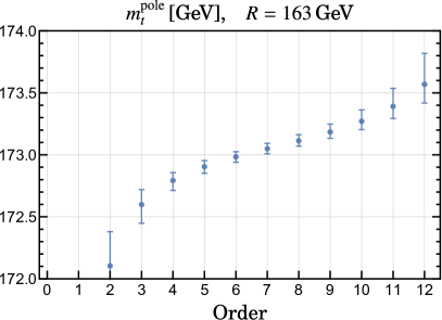
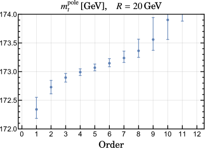
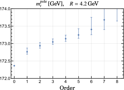
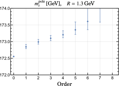
Figure 4: Top quark pole mass $m^{\mathrm{pole}}_{t}$ as a function of the perturbative order for massless bottom and charm quarks, converted from the $\overline{\mathrm{MS}}$ mass (upper left panel) or the MSR mass (other panels) at different scales of $R$. The central dots are obtained for the default renormalization scales for the strong coupling, the error bars represent the scale variation. This corresponds to the black dots and error bars in Fig. 6 of Ref. [2].

Analogous commands can be used to extract the relevant values of the pole mass when converting from the MSR scheme at various scales of $R$. Utilizing these numbers it is now straightforward to reproduce Fig. 6 of Ref. [2] for vanishing bottom and charm mass (black dots in Ref. [2]), see Fig. 4. The asymptotic value which can be assigned to the pole mass lies in the region where the series grows linearly, which is in Fig. 4, roughly in the region around $173$ GeV. This is confirmed by the output of the command MassPoleDetailed, which gives

  In[]:= MassPoleDetailed["t", 6, mtmt, mtmt, "min"]
  Out[]= {173.07508395890844, 0.06445302708283407, 8}

  In[]:= MassPoleDetailed["t", 6, mtmt, mtmt, "range"]
  Out[]= {173.07976320487433, 0.12605058936964042, 8}

  In[]:= MassPoleDetailed["t", 6, mtmt, mtmt, "drange"]
  Out[]= {173.1081654841447, 0.16284602132711257, 8}

for the three methods to estimate the asymptotic pole mass supported by REvolver from the relation between the pole and the MSR mass $m_{t}^{(5)}(\overline{m}_{t})$ at the scale $163$ GeV. While the estimation of the ambiguity can vary by more than a factor of $2$ depending on the employed strategy, the estimated asymptotic pole mass is fairly stable.

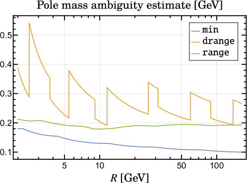
Figure 5: Comparison of the pole mass ambiguity estimating strategies available in REvolver obtained from the series between the pole mass and the running mass $m_{t}^{(5)}(R)=m_{t}^{\rm MSR}(R)$ for the case that all quarks lighter than the top quark are considered to be massless. The figure shows the size of the ambiguity of the top quark pole mass in GeV as estimated by the min (blue lower curve), drange (orange upper curve) and range (green middle curve) strategies over the scale $R$.

Figure 5 shows a comparison of the three strategies of estimating the pole mass ambiguity implemented in REvolver from the perturbative series between the pole mass and the running (MSR) mass $m_{t}^{(5)}(R)=m_{t}^{\rm MSR}(R)$ at the scale $R$. The plot is produced with the command

  In[]:= LogLinearPlot[
          {MassPoleDetailed["t", 6, R, "min"][[2]],
           MassPoleDetailed["t", 6, R, "drange"][[2]],
           MassPoleDetailed["t", 6, R, "range"][[2]]},
          {R, 2, mtmt}, PlotRange -> {0.05, 0.26}]

omitting all options related to plot styling and annotations for brevity.

The figure shows the size of the ambiguity of the top quark pole mass in GeV as estimated by the strategies over the scale $R$, specifying the scale in the perturbative relation between the pole and running mass. All quarks lighter than the top quark are considered to be massless. Due to its discrete nature, the drange method produces a discontinuous curve, while the continuous version range provides a very stable result. The min method leads to an ambiguity estimate that is logarithmically decreasing with $R$.

7.3 Cores with Multiple Massive Quarks

7.3.1 Strong coupling and $\Lambda_{\rm QCD}$

Strong coupling evolution through multiple flavor thresholds

In Ref. [33] the 3-flavor strong coupling value $\alpha_{s}^{(3)}(m_{\tau})$ was determined from hadronic $e^{+}e^{-}$ $R$-ratio data for c.m. energies below the charm production threshold. For this determination, fixed-order (FO) as well as contour-improved (CI) perturbation theory were applied, and the corresponding values $\alpha_{s}^{(3)}(m_{\tau})_{\rm FO}=0.298$ and $\alpha_{s}^{(3)}(m_{\tau})_{\rm CI}=0.304$ were subsequently converted to $\alpha_{s}^{(5)}(m_{Z})$ employing the 4-loop beta function as well as the 3-loop matching relations at the charm and bottom thresholds. The respective values for the strong coupling at the Z-scale were quoted in Eq. (4.7) of that reference as $\alpha_{s}^{(5)}(m_{Z})_{\rm FO}=0.1158$ and $\alpha_{s}^{(5)}(m_{Z})_{\rm CI}=0.1166$, respectively.

For the conversion, the values $\overline{m}_{c}=1.28$ GeV and $\overline{m}_{b}=4.2$ GeV were used for the charm and bottom standard running masses, respectively, and the charm and bottom threshold matching scales were set to $\mu_{c}=2.0$ GeV and $\mu_{b}=4.0$ GeV, respectively. To reproduce the conversion with REvolver we define these input values with

  In[]:= mTau = 1.77686;
         {mcmc, mbmb} = {1.28, 4.2};
         matchList = {2.0/mcmc, 4.0/mbmb};
         {amTauFO, amTauCI} = {0.298, 0.304};

and define one Core for each value of $\alpha_{s}^{(3)}(m_{\tau})$

 In[]:= CoreCreate["FO", 5, {3, amTauFO, mTau},
         {{4, mcmc, mcmc}, {5, mbmb, mbmb}}, runAlpha -> 4,
         orderAlpha -> 3, fMatch -> matchList]
        CoreCreate["CI", 5, {3, amTauCI, mTau},
         {{4, mcmc, mcmc}, {5, mbmb, mbmb}}, runAlpha -> 4,
         orderAlpha -> 3, fMatch -> matchList]

where the parameters relevant for running and matching were set with the optional parameters runAlpha, orderAlpha and fMatch.

The values of $\alpha_{s}^{(5)}(m_{Z})$ can now be easily extracted by

  In[]:= AlphaQCD["FO", mZdef, 5]
         AlphaQCD["CI", mZdef, 5]
  Out[]= 0.11581049250660494
  Out[]= 0.11662117512902259

in full agreement with Eq. (4.7) of Ref. [33].

Similarly, in Ref. [34] $\alpha_{s}^{(3)}(m_{\tau})$ was determined from $\tau$ decay data and converted to $\alpha_{s}^{(5)}(m_{Z})$ employing 4-loop evolution and matching. We update the values for the standard running bottom and charm masses to the ones in the reference paper and define the value of $\alpha_{s}^{(3)}(m_{\tau})$ as given in Eq. (19) therein as well as the associated Core

  In[]:= {mcmc, mbmb} = {1.286, 4.164};
         amTau = 0.332;

  In[]:= CoreDeleteAll[]
         CoreCreate["O", 5, {3, amTau, mTau},
          {{4, mcmc, mcmc}, {5, mbmb, mbmb}}, runAlpha -> 4]

where, following Ref. [34], the strong coupling evolution is set to 4-loop precision. We focus on the central value here for brevity. The value of $\alpha_{s}^{(5)}(m_{Z})$ can now easily be extracted with

  In[]:= AlphaQCD["O", mZdef, 5]
  Out[]= 0.12019776978833413

agreeing with Eq. (20) of Ref. [34].

Flavor number dependence of the QCD scale $\Lambda_{\mathrm{QCD}}^{(n_{f})}$

To demonstrate the capability of REvolver to extract $\Lambda_{\mathrm{QCD}}^{(n_{f})}$ in various flavor number schemes we consider Ref. [35], where $\alpha_{s}^{(5)}(m_{Z})=0.1179$ has been determined by the ALPHA collaboration and values for $\Lambda_{\mathrm{QCD}}^{(nf)}$ with $3\leq n_{f}\leq 5$ were determined, see Eqs. (4.14) as well as (5.3) and (5.4) of that reference.

To reproduce the $\Lambda_{\mathrm{QCD}}^{(n_{f})}$ values with REvolver we create a Core with massive bottom and charm quarks (with standard running mass values taken from the PDG [23]) and define the value of $\alpha_{s}^{(5)}(m_{Z})$ to be the one given in the reference paper

  In[]:= {amZ, mcmc, mbmb} = {0.1179, 1.27, 4.18};

  In[]:= CoreDeleteAll[]
         CoreCreate["O", 5, {5, amZ, mZdef},
          {{4, mcmc, mcmc}, {5, mbmb, mbmb}}]

We now extract $\Lambda_{\mathrm{QCD}}^{(n_{f})}$ in the $n_{f}=5\,,4\,,3$ flavor schemes in the so-called $\overline{\mathrm{MS}}$ scheme [ see Eq. (21) in App. A.2 ] with

  In[]:= LambdaQCD["O", 5]
         LambdaQCD["O", 4]
         LambdaQCD["O", 3]
  Out[]= 0.20745573124097272
  Out[]= 0.288991643859333
  Out[]= 0.33153068987761314

The numbers are in exact agreement with the values shown in Ref. [35].

7.3.2 Top quark running mass at low scales

In Ref. [36] a calibration analysis was provided which suggested that the top quark running mass $m_{t}(1\,\mathrm{GeV})$ agrees within theoretical uncertainties with the MC top mass parameter $m_{t}^{\mathrm{MC}}$ of the Pythia event generator. Specifically, the authors quote a value of $m_{t}(1\,\mathrm{GeV})=172.82\pm 0.19$ GeV for a calibration with $m_{t}^{\mathrm{MC}}=173$ GeV, given in Table 1. That analysis was carried out in the approximation of massless bottom and charm quarks. Here we demonstrate how REvolver can be used to investigate how finite charm and bottom quark masses affect the value of the standard running mass $\overline{m}_{t}$ calculated from $m_{t}(1\,\mathrm{GeV})$. As an estimate of the uncertainties we quote the difference of the values computed using $4$- and $3$-loop R-evolution.

To this end we create six Cores: two with massless bottom and charm quarks, two with a massless charm quark and a massive bottom quark, and two with massive bottom and charm quarks, employing $\overline{m}_{c}=1.27$ GeV and $\overline{m}_{b}=4.18$ GeV for the standard running charm and bottom quark masses. Among the two respective Cores one employs 3-loop and the other 4-loop precision for the R-evolution equation:

  In[]:= {mcmc, mbmb, mt1} = {1.27, 4.18, 172.82};

  In[]:= CoreDeleteAll[]
         CoreCreate["t4", 6, {5, amZdef, mZdef}, {{5, mt1, 1}},
          runMSR -> 4]
         CoreCreate["t3", 6, {5, amZdef, mZdef}, {{5, mt1, 1}},
          runMSR -> 3]
         CoreCreate["bt4", 6, {5, amZdef, mZdef},
          {{5, mbmb, mbmb}, {4, mt1, 1}}, runMSR -> 4]
         CoreCreate["bt3", 6, {5, amZdef, mZdef},
          {{5, mbmb, mbmb}, {4, mt1, 1}}, runMSR -> 3]
         CoreCreate["cbt4", 6, {5, amZdef, mZdef},
          {{4, mcmc, mcmc}, {5, mbmb, mbmb}, {3, mt1, 1}},
          runMSR -> 4]
         CoreCreate["cbt3", 6, {5, amZdef, mZdef},
         {{4, mcmc, mcmc}, {5, mbmb, mbmb}, {3, mt1, 1}},
         runMSR -> 3]

The Core setups specify that $m_{t}^{\rm MSR}(1\,\mbox{GeV})=172.82$ GeV is the running top quark mass in the scheme in which all massive flavors above the scale of $1$ GeV are integrated out. It is easy to extract the top quark standard running masses and their uncertainties from the Cores above with

  In[]:= MassMS["t4", 6]
         MassMS["t4", 6] - MassMS["t3", 6]
  Out[]= 163.00308510782256
  Out[]= 0.05105270648016358

  In[]:= MassMS["bt4", 6]
         MassMS["bt4", 6] - MassMS["bt3", 6]
  Out[]= 162.94352028117146
  Out[]= 0.050962554040836494

  In[]:= MassMS["cbt4", 6]
         MassMS["cbt4", 6] - MassMS["cbt3", 6]
  Out[]= 162.92268002391415
  Out[]= 0.049529435610025985

where the first numbers refer to the setup with massless bottom and charm quarks and the last ones to the one where bottom and charm quarks have mass.

We observe that the finite bottom mass lowers the standard top running mass by around $60$ MeV and the finite charm mass decreases the standard top running mass by about another $20$ MeV. The perturbative uncertainty of the conversion amounts to around $50$ MeV in all cases. Together, the finite charm and bottom masses lower the standard running top mass by about $80$ MeV, which is larger than the perturbative uncertainty.

7.3.3 Charm mass effects for the bottom quark mass

To demonstrate the effect of lighter massive flavors in conversions between short-distance mass schemes we consider Ref. [37], where effects of the finite charm quark mass on bottom quark mass determinations from $\Upsilon$ mesons were (calculated and) examined. In Eq. (99) of that paper the bottom standard running mass is computed from the 1S mass $m_{b}^{\mathrm{1S}}=4.7$ GeV with and without the contribution of the charm standard running quark mass $\overline{m}_{c}=1.5$ GeV. The strong coupling value was set to $\alpha_{s}^{(4)}(m_{b}^{\mathrm{1S}})=0.216$. We define these parameters with

  In[]:= {mb1S, mcmc, amb1S} = {4.7, 1.5, 0.216};

and create two 4-flavor Cores, one with a massless charm quark and one with the charm mass given above

  In[]:= CoreDeleteAll[]
         CoreCreate["c0", {4, amb1S, mb1S}]
         CoreCreate["cm", 4, {4, amb1S, mb1S},
          {{4, mcmc, mcmc}}]

We then create two additional Cores by adding the bottom quark 1S mass $m_{b}^{\mathrm{1S}}=4.7$ GeV to the existing Cores, where, following Ref. [37], the perturbative order of its relation to the standard running mass is $\mathcal{O}(\alpha_{s}^{3})$ and the relativistic (“upsilon-expansion”) counting scheme is adopted.

  In[]:= Add1SMass["c0", "bc0", mb1S, 5, mb1S, "relativistic",
          mb1S, 3]
         Add1SMass["cm", "bcm", mb1S, 5, mb1S, "relativistic",
          mb1S, 3]

We have furthermore set the running mass scale and the renormalization scale of the strong coupling to $m_{b}^{\mathrm{1S}}$ and the parameter nfConv to $5$ to specify direct conversion without R-evolution to be in accordance with the computation carried out in Ref. [37].

Extracting the standard mass from the massless charm Core gives

  In[]:= MassMS["bc0", 5]
  Out[]= 4.190311348710497

in perfect agreement with $\overline{m}_{b}=(4.7-0.382-0.098-0.030)\,\mathrm{GeV}=4.190$ GeV as quoted in Ref. [37]. For the standard mass from the massive charm Core we get

  In[]:= MassMS["bcm", 5]
  Out[]= 4.178691644159289

with a sub-MeV difference to the reference value $\overline{m}_{b}=(4.7-0.382-(0.098+0.0072)-(0.03+0.0049))\,\mathrm{GeV}=4.178$ GeV.

7.3.4 Top quark pole masses

In the following we investigate the influence of massive bottom and charm quarks on the perturbative series relating the top quark standard running mass and the pole mass.

Pole-$\overline{\mathrm{MS}}$ mass series dependence on lighter massive quarks

In Ref. [2] the dependence of the high-order asymptotic series for the top quark pole-$\overline{\mathrm{MS}}$ mass relation on finite bottom and charm quark mass was examined and an algorithm to determine explicit analytic formulae (accounting for the semianalytical results given in Ref. [38]) were provided, which are implemented in REvolver. Explicit results for the asymptotic series coefficients beyond ${\cal O}(\alpha_{s}^{4})$ were provided in Ref. [2] for the scenarios of massless bottom and charm quarks, massive bottom and massless charm quarks as well as massive bottom and charm quarks. To compare the results of REvolver to those of Ref. [2] we set the appropriate relevant parameters for the standard running charm, bottom and top quark masses as well as for the strong coupling and create the Cores for the three scenarios

  In[]:= {mcmc, mbmb, mtmt} = {1.3, 4.2, 163};
         {amZ, mZ} = {0.118, 91.187};

  In[]:= CoreDeleteAll[]
         CoreCreate["tbc", 6, {5, amZ, mZ},
          {{4, mcmc, mcmc}, {5, mbmb, mbmb}, {6, mtmt, mtmt}}]
         CoreCreate["tb", 6, {5, amZ, mZ},
          {{5, mbmb, mbmb}, {6, mtmt, mtmt}}]
         CoreCreate["t", 6, {5, amZ, mZ}, {{6, mtmt, mtmt}}]

The perturbative series relating the standard running mass and the pole mass can be generated as shown in Sec. 7.2.6 and depicted in the upper left panel of Fig. 4 for massless bottom and charm quarks. In Fig. 6 we show the result of repeating this procedure for each of the Cores created above. It is clearly visible that for each additional accounted massive quark flavor the series diverges faster and consequently the respective pole mass ambiguity increases.

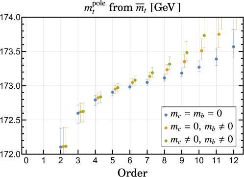
Figure 6: Top quark pole mass $m^{\mathrm{pole}}_{t}$ as a function of the perturbative order with bottom and charm quark masses set to zero (left blue), massless charm quark (middle orange) and massive bottom and charm masses (right green). The conversion is performed from the $\overline{\mathrm{MS}}$ mass. The central dots are obtained for the default renormalization scales for the strong coupling $\mu=\overline{m}_{t}$, the error bars represent the scale variation $\overline{m}_{t}/2\leq\mu\leq 2\,\overline{m}_{t}$.

In accordance with Ref. [2] we read out the value of the asymptotic top quark pole mass, the associated ambiguity and the order of the minimal correction term from each Core employing the drange approach, which is based on all series terms in the superasymptotic region, by executing

  In[]:= MassPoleDetailed["t", 6, mtmt, "drange"]
         MassPoleDetailed["tb", 6, mtmt, "drange"]
         MassPoleDetailed["tbc", 6, mtmt, "drange"]
  Out[]= {173.09649964256326, 0.16178589168021063, 8}
  Out[]= {173.17525229067104, 0.2336983055654116, 7}
  Out[]= {173.17973196293923, 0.26632540751468525, 7}

The three results agree with the numbers given in Table 5 of Ref. [2] within uncertainties.

We now return to Ref. [3]. There, finite charm and bottom quark mass effects on the value of the top quark asymptotic pole mass were quantified by an approximate and heuristic method utilizing order-dependent light flavor decoupling in the strong coupling. A numerical value for the resulting ambiguity of the asymptotic pole mass was quoted in Eq. (5.1) of that paper using size of the minimal correction of the asymptotic series.

Fixing the value of the top, bottom and charm quark standard running masses to the values given in Ref. [3] and creating an associated Core

  In[]:= {mtmt, mbmb, mcmc} = {163.508, 4.2, 1.3};

  In[]:= CoreCreate["tbc2", 6, {5, amZdef, mZdef},
          {{4, mcmc, mcmc}, {5, mbmb, mbmb}, {6, mtmt, mtmt}}]

we obtain

  In[]:= MassPoleDetailed["tbc2", 6, mtmt, mtmt, "min"]
  Out[]= {173.61531203486197, 0.10050070355543994, 7}

where we employ the min method to match the approach used in Ref. [3]. The asymptotic pole mass value and the associated ambiguity are quoted as $173.667$ GeV and $108$ MeV, respectively, in that reference and differs by around $50$ and $8$ MeV, respectively, to the result provided by REvolver. The difference is mainly related to the exact treatment of light massive flavor corrections provided by REvolver.

Normalization of the pole mass renormalon

Finally, we demonstrate REvolver’s capability to compute the normalization $N_{1/2}^{(n_{\ell})}$ of the pole mass renormalon for a given number $n_{\ell}$ of massless quark flavors. Reusing the Cores created in one of the previous examples, the value of the normalization for $n_{\ell}=3,4,5$ can be extracted with

  In[]:= N12[#] & /@ {"tbc","tb","t"}
  Out[]= {0.5371120004494861, 0.5055628679671248,
          0.4612967890971816}

in excellent agreement with the corresponding values $N_{1/2}^{(n_{\ell}=3,4,5)}=\{0.5370\pm 0.0011,\,0.5056\pm 0.0015,\,0.4616\pm 0.0020\}$ given for $\mu/\overline{m}=1$ in Table 1 of Ref. [3].

In Eq. (2.21) of Ref. [2] the $\lambda$-parameter was varied in the range $1/2\leq\lambda\leq 2$, and the associated central value and uncertainty of the renormalon normalization $N_{1/2}^{(n_{\ell})}$ were determined. The corresponding values for $n_{\ell}=3,4,5$ can be reproduced by REvolver with

  In[]:= list2 = 2^Range[-1, 1, 2/19];

  In[]:= N3Tab = N12["tbc", #] & /@ list2;
         (Max[N3Tab] + {1, -1} * Min[N3Tab])/2
  Out[]= {0.5256087104548577, 0.011913515642471062}

  In[]:= N4Tab = N12["tb", #] & /@ list2;
         (Max[N4Tab] + {1, -1} * Min[N4Tab])/2
  Out[]= {0.4916415824077933, 0.016342715842279004}

  In[]:= N5Tab = N12["t", #] & /@ list2;
         (Max[N5Tab] + {1, -1} * Min[N5Tab])/2
  Out[]= {0.44606744334202203, 0.023867353429116556}

in perfect agreement with the values $N_{1/2}^{(n_{\ell}=3,4,5)}=\{0.526\pm 0.012,\,0.492\pm 0.016,\,0.446\pm 0.024\}$, quoted in Eq. (2.21) of Ref. [2].

8 Theoretical input

The perturbative coefficients of the QCD $\beta$-function, that is the renormalization group equation of the $\overline{\rm MS}$ strong coupling $\alpha_{s}^{(n_{f})}(\mu)$ in a given $n_{f}$ flavor number scheme, are known to five loops and can be found in Refs. [39, 40, 41, 42, 43, 44, 45, 46]. If REvolver is used for scenarios with massless quarks only, it is recommended to cite those references. The perturbative coefficients for the strong coupling flavor matching relation at the quark thresholds are known up to four loops and can be found in Refs. [47, 48, 49, 50]. If REvolver is used for strong coupling evaluations in different flavor number schemes involving massive quark threshold matching, these references should be cited.

The perturbative coefficients of the relation between the $\overline{\rm MS}$ mass $\overline{m}_{q}^{(n_{f})}(\mu)$, for the case where $n_{f}-1$ is the number of flavors lighter than the massive quark $q$, and the pole mass $m^{\rm pole}_{q}$ for the case that all lighter quarks are massless, are known to four loops and can be found in Refs. [51, 52, 53, 12]. If REvolver is used to compute relations between the $\overline{\rm MS}$ mass and the pole mass when all lighter quarks are massless, these references should be included. The two- and three-loop corrections coming from the masses of lighter massive quarks can be found in Refs. [52] and [38, 54], respectively. It would be appropriate to also cite these references, if REvolver is used to compute lighter massive flavor effects in the relation between the $\overline{\rm MS}$ mass and the pole mass of a heavy quark. The perturbative coefficients of the $\overline{\rm MS}$ mass renormalization group equations (relevant for renormalization scales above the mass of quark $q$) are known to five loops and can be found in Refs. [55, 56, 57, 58]. These references should be cited whenever the code is used to compute the running of the $\overline{\rm MS}$ mass in any flavor scheme that includes the heavy quark itself. The perturbative coefficients of the flavor matching relations needed when the running $\overline{\rm MS}$ mass evolves to scales beyond even heavier massive quarks are known up to four loops and can be found in Refs. [47, 59]. These references should be included, if the $\overline{\rm MS}$ mass is evaluated in different flavor number schemes involving threshold matching associated to even heavier massive quarks.

The MSR mass $m_{q}^{{\rm MSR},(n_{\ell})}(\mu)$ is derived from the perturbative relation between the pole mass and the standard running mass $\overline{m}_{q}$ by integrating out the quark flavor $q$, see Sec. 3. Thus, all perturbative properties of the MSR mass are derived from expressions known for the $\overline{\rm MS}$ scheme from the references mentioned in the previous paragraph. The MSR mass concept was first suggested in Ref. [6] and allows to consistently consider renormalization group evolution for scales $\mu$ below the quark mass $m_{q}$, called “R-evolution”. The perturbative coefficients of (i) the relation between the MSR mass $m_{q}^{{\rm MSR},(n_{\ell})}(\mu)$, where $n_{\ell}$ is smaller or equal to the number of flavors lighter than the massive quark $q$, and the pole mass $m^{\rm pole}_{q}$, (ii) the matching relation of the MSR mass to the $\overline{\rm MS}$ mass, and (iii) its $n_{\ell}$ flavor-number-dependent renormalization group equation for the case that all lighter quarks are massless (which are all known to four loops) can be found in Ref. [1]. The MSR mass scheme implemented in REvolver is called the “natural” MSR mass scheme in Ref. [1]. The two- and three-loop corrections coming from the masses of lighter massive quarks including the flavor matching relations, when the MSR mass evolution crosses a lighter massive quark threshold, can be found in Ref. [2]. The results for the lighter massive quark effects given in Ref. [2] involve a parametrization of the results provided in Ref. [38] (in terms of coefficients $\delta_{2}$ and $\delta_{Q,n}^{(q,q^{\prime},\ldots)}$) that accounts for theoretical interrelations of the different contributions not considered in Ref. [38], and allows for a straightforward generalization for the case of multiple lighter massive quark flavors. The parametrization is also fully compatible with the recent analytic updates on the three-loop corrections given Ref. [54] within a few MeV. The expression for $\delta_{2}$ used in REvolver has been given in Ref. [2]. The concrete expressions for the other coefficients $\delta_{Q,n}^{(q,q^{\prime},\ldots)}$ have been taken from Ref. [60]. If REvolver is used to calculate the MSR mass of a massive quark in the case that all lighter quarks are massless, Refs. [1, 2] should be cited. If REvolver is used to calculate the MSR mass in different flavor number schemes involving flavor threshold matching as light massive quark thresholds Ref. [2] should be cited. The possibility to resum (large) logarithms in the relation between short-distance quark mass definitions involving scales below the quark mass scale (e.g. concerning the ratio of the heavy quark mass and a lighter quark mass) is currently only provided through the MSR mass, which is therefore the primary short-distance mass scheme for scales below the quark masses contained in the REvolver core objects. If REvolver is used to resum such logarithms in the relation of short-distance masses (even not involving the MSR directly), this MSR mass functionality is used as an intermediate step, and it is appropriate to cite Ref. [1, 6].

The quark mass dependence of the formulae of the flavor threshold matching relations for the flavor-number-dependent strong coupling $\alpha_{s}^{(n_{f})}(\mu)$, the $\overline{\rm MS}$ mass $\overline{m}_{q}^{(n_{f})}(\mu)$ and the MSR mass $m_{q}^{{\rm MSR},(n_{\ell})}(\mu)$ implemented in REvolver are expressed in terms of the standard running mass $\overline{m}_{q}$. Changing the scheme of the quark mass in these matching relations is not supported in REvolver because the corresponding numerical impact is tiny and negligible for practical applications where large logarithmic corrections are properly resummed.

The perturbative coefficients of the relation between the kinetic and pole mass, assuming lighter massive quarks to be massless, can be found in Refs. [17, 21]. The 1S mass scheme was first suggested in Refs. [15, 14]. The perturbative coefficients for the 1S mass scheme have been derived in Refs. [15, 14, 61, 19, 62, 63, 64]. The perturbative coefficient for the PS mass scheme, first suggested in Ref. [18], can be obtained from Refs. [18, 19] using analytic results for the static potential as given in Refs. [65, 66, 67, 68, 69, 70, 71]. The relation connecting the RS and pole mass schemes is described in Refs. [30, 20] and references therein. Whenever values for any of these masses are obtained through REvolver, the corresponding references should be mentioned. The lighter massive flavor corrections in the relation to the pole mass are known for the kinetic [22], 1S [72, 73] and PS masses [74]. For the 1S mass REvolver currently only accounts for the fixed-order corrections in the relation to the pole mass. Therefore, if lighter quarks are considered massive, the appropriate references should be cited.

To compute the RGI mass [13] the standard formula is evaluated as described below Eq. (28).

9 Summary

In this article we have presented REvolver, a C++ library for carrying out state-of-the-art renormalization group evolution and flavor matching for the QCD coupling and quark masses, and conversion between the most common quark mass renormalization schemes. For short-distance quark masses the achievable precision is at the level of $10$ to $20$ MeV. In addition to similar libraries that are already available REvolver offers the Core concept, that allows to define and manage different physical scenarios for coupling and quark mass values, and to carry out renormalization group summation of logarithms from scales above and below the quark masses. REvolver supports, in particular, the summation of logarithms described by the R-evolution equation, which describes the linear scale evolution characteristic to low-scale short-distance masses, and it accounts for the flavor threshold corrections that arise in this linear scale evolution. Furthermore, REvolver provides access to the asymptotic perturbative relations to the pole mass to in principle any perturbative order, and it provides quasi-exact solutions to the renormalization group equations (i.e. exact up to machine-precision) for complex renormalization scales. The REvolver library can be also accessed through Mathematica and Python interfaces. We have provided a large number of examples for the most common applications, which are shipped along with the library in the form of Mathematica and Jupyter notebooks, as well as a C++ program.

Appendix A Algorithms to Solve the Differential Equations

In this appendix some details on the algorithms used in REvolver are provided.

A.1 Core Creation

For the creation of a Core, values for the strong coupling and the running masses of the $n_{q}$ massive quarks at specified scales and in specified flavor-number schemes, as well as the total number of flavors $n_{T}$, are provided by the user. Let us call the corresponding tuples $\{n_{\alpha},\alpha_{s}^{(n_{\alpha})}(\mu_{\alpha})$, $\mu_{\alpha}\}$ for the strong coupling and $\{k_{n},m_{q_{n}}^{(k_{n})}(R_{n}),R_{n}\}$, with $\max[k_{n},n_{\alpha}]\leq n_{T}$, $1\leq n\leq n_{q}$, for the $n_{q}$ massive quarks, where $q_{1}$ refers to the lightest and $q_{n_{q}}$ to the heaviest massive quark. In a first step REvolver determines the values of the standard running masses $\overline{m}_{q_{n}}$. Subsequently, the following strong coupling and running mass values at each flavor threshold matching scale $\mu_{n}$ are obtained: $\alpha_{s}^{(n_{T}+n-1-n_{q})}(\mu_{n})$, $\alpha_{s}^{(n_{T}+n-n_{q})}(\mu_{n})$ and $m_{n}^{(n_{T}+n-1-n_{q})}(\mu_{n})$, $m_{n}^{(n_{T}+n-n_{q})}(\mu_{n})$. These numbers serve as the initial conditions to compute $\alpha_{s}$ and the running masses $m_{q_{n}}$ at any renormalization scale and in any specified flavor-number scheme. We have implemented into our code a fast multi-dimensional recursive algorithm that solves the coupled system of equations to the specified precision.

The determination of the standard running masses $\overline{m}_{q_{n}}$ in the algorithm is particularly important since the flavor matching scales $\mu_{n}$ are specified as dimensionless coefficients times $\overline{m}_{q_{n}}$. If at the $i$-th iteration the standard running masses are $[\overline{m}_{q_{n}}]_{i}$, the numerical values $[\overline{m}_{q_{n}}]_{i+1}$ at step $(i+1)$ are computed evolving (and matching if necessary) the quark masses $m_{q_{n}}^{(k_{n})}(R_{n})$ from the user-specified $\mu=R_{n}$, for which the numerical value of the mass was provided, to $\mu=[\overline{m}_{q_{n}}]_{i}$. To do that, before running the masses, the program computes the values of $\alpha_{s}$ at the various thresholds $\mu_{n}$ using $[\overline{m}_{q_{n}}]_{i}$ as well. After each iteration is carried out, the new standard running masses are compared to the previous ones, and if their largest relative deviation is smaller than the required precision, the process stops. In the initial step it is assumed that $[\overline{m}_{q_{n}}]_{i=0}=m_{q_{n}}^{(k_{n})}(R_{n})$. We checked that the algorithm is very robust and converges quickly even for very extreme starting conditions such as a charm quark mass defined with $k_{1}=6$ active flavors taking for $R_{1}$ a very large scale, together with a top quark mass defined at $R_{3}=1\,$GeV with $k_{3}=3$ active flavors. There is the possibility that the algorithm does not converge, if a particular sequence of $[\overline{m}_{q_{n}}]_{i}$-values repeats itself. This is avoided by adopting, after the $20$-th iteration ($i\geq 21$) the linear combination $(1-\mathtt{damp})[\overline{m}_{q_{n}}]_{i}+\mathtt{damp}[\overline{m}_{q_{n}}]_{i-1}$, with damp being a random number between $0$ and $0.2$, as the outcome of the $i$-th iteration.

To compute the strong coupling flavor matching REvolver takes as exact the upward relation (at the user-specified loop order)

$$\alpha^{(n_{\ell}+1)}_{s}(\mu_{n})=\alpha^{(n_{\ell})}_{s}(\mu_{n})\Biggl{\{}1+\sum_{i=1}\biggl{[}\frac{\alpha^{(n_{\ell})}_{s}(\mu_{n})}{4\pi}\biggr{]}^{i}\xi_{i}(n_{\ell})\Biggr{\}},$$ (9)

where $\xi_{i}$ may depend on $\log(\overline{m}_{q_{n}}/\mu_{n})$. This means that the values for $\alpha_{s}^{\!(n_{\ell})}\!(\mu_{n})$ and $\alpha_{s}^{(n_{\ell}+1)}(\mu_{n})$ in REvolver always satisfy exactly Eq. (9). If $\alpha_{s}^{(n_{\ell})}(\mu_{n})$ is given, the value of $\alpha_{s}^{(n_{\ell}+1)}(\mu_{n})$ is computed directly from Eq. (9). If, on the contrary, $\alpha_{s}^{(n_{\ell}+1)}(\mu_{n})$ is given and $\alpha_{s}^{(n_{\ell})}(\mu_{n})$ shall be obtained, our program numerically inverts Eq. (9) in an iterative way as described in the following. For simplicity we omit the argument $\mu_{n}$ and write $[\alpha^{(n_{\ell})}]_{k}$ for the $k$-th iteration value. The value at the $(k+1)$-th step the reads

$$[\alpha^{(n_{\ell})}]_{k+1}=\frac{\alpha_{s}^{(n_{\ell}+1)}(\mu_{n})}{1+\sum_{i=1}\Bigl{(}\frac{[\alpha^{(n_{\ell})}]_{k}}{4\pi}\Bigr{)}^{\!i}\,\xi_{i}(n_{\ell})}\,,$$ (10)

where for the first iteration $[\alpha^{(n_{\ell})}]_{k=0}=\alpha_{s}^{(n_{\ell}+1)}(\mu_{n})$ is adopted. The algorithm converges very quickly, even for $\alpha_{s}^{(n_{\ell}+1)}(\mu_{n})$ values as large as $0.69$. For smaller values of the strong coupling, and specially if $\mu_{n}\simeq\overline{m}_{q_{n}}$, the RHS of Eq. (10) is very weakly depending on $\alpha^{(n_{\ell})}_{k}$ (since the 1-loop term is very small or vanishing) and only a few iterations are necessary. If $\alpha_{s}^{(n_{\ell}+1)}(\mu_{n})$ is larger than $0.69$, there is no solution to Eq. (9) and the iterative procedure will fail. In those cases the program will return the leading order solution $\alpha_{s}^{(n_{\ell})}(\mu_{n})=\alpha_{s}^{(n_{\ell}+1)}(\mu_{n})$. If the solution exists, the algorithm converges as well, because the slope of the left-hand-side is smaller than unity in absolute value.

A.2 Strong Coupling

For the QCD $\beta$-function at $N$-loop order (where $N$ is the integer value specified in the variable runAlpha), see Eq. (6), the coefficients $b_{i}$ are defined by

$$\beta^{N}_{\rm{QCD}}(\alpha_{s})\equiv-\frac{\alpha^{2}_{s}}{2\pi}\beta_{0}\biggl{[}1+\sum_{i=1}^{N-1}\Bigl{(}\frac{\alpha_{s}}{4\pi}\Bigr{)}^{\!\!i}\,b_{i}\biggr{]},\qquad b_{i}\equiv\frac{\beta_{i}}{\beta_{0}}\,.$$ (11)

The algorithms implemented in REvolver provide solutions for the strong coupling differential equation based on the $N$-loop $\beta$-function that are numerically exact (within the specified precision) and do not involve any additional approximation related to $N$-loop precision. The associated coefficients $c^{N}_{n}$, which parametrize the associated inverse QCD $\beta$-function, are defined by

$$\frac{1}{\beta^{N}_{\rm{QCD}}(\alpha_{s})}=-\frac{2\pi}{\beta_{0}}\frac{1}{\alpha^{2}_{s}}\biggl{[}1+\sum_{i=1}c^{N}_{i}\Bigl{(}\frac{\alpha_{s}}{4\pi}\Bigr{)}^{\!\!i}\,\biggr{]},$$ (12)

where, except for $N=1$, the sum extends to infinity even though there is a finite limit $N$ in the sum defining $\beta^{N}_{\rm{QCD}}$ (for $N=1$ one has $c^{N}_{i}=0$ for all $i\geq 1$). The (infinite set of) $c^{N}_{i}$ coefficients can be computed in terms of $N-1$ coefficients $b_{1},\ldots b_{N-1}$ using the recursive relation shown in Eq. (13). The convergence radius of the series is set by the distance from the origin to the nearest pole in the complex plane, which is equivalent to the smallest module of the $\beta$-function roots (excluding the double pole at the origin), which are in general complex numbers. Hence the convergence radius depends both on the number of flavors and the loop order $N$. It increases with the number of flavors and decreases with the loop order $N$, and in all cases is much larger than any physical value of $\alpha_{s}$ that may arise in phenomenological applications.

For convenience we define $b_{0}=c^{N}_{0}=1$, which allows to write

$$c^{N}_{n+1}=-\!\!\!\!\sum_{i=1}^{\min(N-1,n+1)}\!\!c^{N}_{n+1-i}\,b_{i}\,.$$ (13)

Many analytic formulae implemented in REvolver use the $t$-variable formalism [6, 1] which is based on the definition

$$t=-\frac{2\pi}{\beta_{0}}\frac{1}{\alpha_{s}}\,,$$ (14)

which gives the relation

$${\rm d}\ln(\mu)=-\hat{b}^{N}\!(t)\,{\rm d}t\,,$$ (15)

for the renormalization scale $\mu$ where

$$\hat{b}^{N}\!(t)=-\frac{2\pi}{\beta_{0}\,t^{2}\beta^{N}_{\rm{QCD}}\bigl{(}-\frac{2\pi}{\beta_{0}}\frac{1}{t}\bigr{)}}\equiv 1+\sum_{i=1}\hat{b}^{N}_{i}\,t^{-i}\,,$$ (16)

with $\hat{b}^{N}_{n}=(-1)^{n}c^{N}_{n}/(2\beta_{0})^{n}$, which implies $\hat{b}^{N}_{0}=1$. The $c_{n}^{N}$ and $\hat{b}_{n}^{N}$ coefficients are obtained numerically whenever needed and stored in a member vector (whose length is extended if necessary) such that they are not re-computed again when used later. For the integral of Eq. (15) it is useful to define the following polynomial in $1/t$ expressed in terms of $\hat{b}_{i}^{N}$:

$$\tilde{G}^{N}\!(t)\equiv\int_{-\infty}^{t}\text{d}t^{\prime}\biggl{[}\hat{b}^{N}(t^{\prime})-1-\frac{\hat{b}^{N}_{1}}{t^{\prime}}\,\biggr{]}=-\sum_{n=1}\frac{\hat{b}^{N}_{n+1}}{n}\,t^{-n}\,.$$ (17)

For $N=1$ one has $\tilde{G}^{N}\!(t)=0$ while for $N\geq 2$ the sum in $\tilde{G}^{N}\!(t)$ always extends to infinity. The exponential of this expression defines the coefficients $g_{\ell}^{N}$ upon reexpansion in powers of $1/t$, $e^{\tilde{G}^{N}(t)}\equiv\sum_{\ell=0}g^{N}_{\ell}(-t)^{-\ell}$, which can be computed with the recursive relation

$$g^{N}_{n+1}=\frac{1}{n+1}\sum_{i=0}^{n}(-1)^{i}\,\hat{b}^{N}_{i+2}\,g^{N}_{n-i}\,,$$ (18)

where ${g}^{N}_{0}=1$. It is also necessary to define the coefficients that result from expanding $e^{-\tilde{G}^{N}(t)}\equiv\sum_{\ell=0}\tilde{g}^{N}_{\ell}(-t)^{-\ell}$ in an analogous way. They can be computed with a very similar recursive algorithm

$$\tilde{g}^{N}_{n+1}=-\frac{1}{n+1}\sum_{i=0}^{n}(-1)^{i}\,\hat{b}^{N}_{i+2}\,\tilde{g}^{N}_{n-i}\,,$$ (19)

where $\tilde{g}^{N}_{0}=1$. Once again one has $g_{n}^{N}=\tilde{g}_{n}^{N}=0$ for $n\geq 1$ when $N=1$. Both $g$ and $\tilde{g}$ coefficients are computed when first needed and then are conveniently stored in member vectors for later use.

The QCD scale $\Lambda_{\rm QCD,t}$ in the t-scheme [1] is defined by

$$\Lambda^{N}_{\rm{QCD,t}}=\mu\,e^{G^{N}\!\bigl{(}-\frac{2\pi}{\beta_{0}}\frac{1}{\alpha_{s}(\mu)}\bigr{)}}\,,$$ (20)

where $G^{N}\!(t)=t+\hat{b}^{N}_{1}\log(-t)+\tilde{G}^{N}(t)$ (where we recall that $\hat{b}_{i>0}^{N}=0$ if $N=1$). The summation for the function $\tilde{G}^{N}$ in Eq. (17) is terminated after the relative size of the last term compared to the associated partial sum is smaller than the specified precision. Since in the evaluation of Eq. (20) the exact solution of the strong coupling differential equation with $N$-loop $\beta$-function $\beta^{N}_{\rm QCD}$ (see next section) for $\alpha_{s}(\mu)$ is used, the numerical value of $\Lambda^{N}_{\rm QCD}$ does (within the specified precision) not depend on $\mu$. For the evaluation in REvolver the value $\mu=100$ GeV is always used. The values for the QCD scale are computed for each number of active flavors and stored as members of the class. For cases in which $\alpha_{s}$ is very large, the sum $G^{N}$ may not converge within the specified precision after adding $200$ terms and REvolver will return NaN (see below why the limit is set to $200$). Again, this only happens for unphysical $\alpha_{s}$ values.

For the QCD scale in the $\overline{\mathrm{MS}}$ definition, $\Lambda_{\rm QCD,\overline{\mathrm{MS}}}$ (following [23]), we use the formula

$$\Lambda^{N}_{\rm{QCD,\overline{\mathrm{MS}}}}=2^{\hat{b}^{N}_{1}}\,\Lambda^{N}_{\rm{QCD,t}}\,,$$ (21)

therefore both schemes coincide for $N=1$.

The algorithm used by REvolver to solve the differential equation for the strong coupling is based on variable separation. Defining $\ell_{\mu}\equiv\log(\mu/\mu_{0})$, $\alpha_{\mu}\equiv\alpha_{s}(\mu)$, $\alpha_{0}\equiv\alpha_{s}(\mu_{0})$ and $a\equiv\alpha_{s}/(4\pi)$ one can expand $1/\beta_{\rm QCD}^{N}$ as in Eq. (12) and integrate term by term. This gives

$$\ell_{\mu}=\!\!\int_{\alpha_{0}}^{\alpha_{\mu}}\!\!\!\frac{\text{d}\alpha}{\beta^{N}_{\rm{QCD}}(\alpha)}=\!-\frac{1}{2\beta_{0}}\biggl{[}\frac{1}{a_{0}}-\frac{1}{a_{\mu}}+c_{1}^{N}\log\!\biggl{(}\frac{a_{\mu}}{a_{0}}\biggr{)}+\!\sum_{i=1}\frac{c^{N}_{i+1}}{i}(a_{\mu}^{i}-a_{0}^{i})\biggr{]}.$$ (22)

where the sum on the RHS is carried out until the last term added is smaller than the specified precision.

We now describe the algorithm to determine $a_{\mu}$ from the algebraic equation (22). At leading-log (LL), i.e. using the 1-loop $\beta$-function ($N=1$), one has $\beta_{n>0}=0$ and the solution is $a^{\rm LL}_{\mu}=a_{0}/(1+2\beta_{0}a_{0}\ell_{\mu})$. For $N\geq 2$ the LL solution is used to rewrite Eq. (22) in the form

$$\frac{1}{a_{\mu}}=\frac{1}{a^{\rm{LL}}_{\mu}}+c_{1}^{N}\log\biggl{(}\frac{a_{\mu}}{a_{0}}\biggr{)}+\sum_{i=1}\frac{c^{N}_{i+1}}{i}(a_{\mu}^{i}-a_{0}^{i})\,,$$ (23)

which is solved recursively. In this iterative procedure, the $(n+1)$-th iteration value for the $N$-loop strong coupling is obtained from the $n$-th iteration one by the relation

$$[a_{\mu}]_{n+1}=\frac{1}{\frac{1}{a^{\rm LL}_{\mu}}+c_{1}^{N}\log\Bigl{(}\frac{[a_{\mu}]_{n}}{a_{0}}\Bigr{)}+\sum_{i=1}\frac{c^{N}_{i+1}}{i}[([a_{\mu}]_{n})^{i}-a_{0}^{i}]}\,.$$ (24)

With the initial choice $[a_{\mu}]^{N}_{0}\equiv a^{\rm{LL}}_{\mu}$ it is ensured that the correct solution is obtained in all cases. The iterative method converges provided that (i) the solution exists and (ii) the (absolute value of the) slope of the right-hand-side function is smaller than $1$. The second condition is always satisfied, and the former will be discussed later in this paragraph. Since $\beta_{1}>0$ we have that $a_{\mu}^{\rm LL}<a_{\mu}$, and the solution beyond 1-loop order is approached from below. The iterative procedure is carried out until the numerical value of $a_{\mu}$ does not change within the specified precision, with a maximum allowed number of $200$ iterations.

The convergence radius for the infinite sum over $c_{i+1}^{N}$ in Eq. (24) is the same as for the inverse $\beta$-function in Eq. (12). However, due to technical limitations related to double-precision floating numbers, REvolver cannot carry out the sum for $\alpha_{s}$ values arbitrarily close to the convergence radius within the specified precision. If after adding $200$ terms this precision is not met, the recursive procedure to obtain $\alpha_{s}$ will stop and NaN will be returned. This happens for $\alpha_{s}\gtrsim 0.7$, hence outside the range of any physical application.

A.3 $\overline{\rm MS}$ and RGI masses

The $K$-loop renormalization group equation (where $K$ is the integer value specified in the variable runMSbar) for the $\overline{\rm MS}$ quark mass $\overline{m}_{q}(\mu)$ has the form

$$\frac{\mathrm{\text{d}}\,\overline{m}_{q}(\mu)}{\mathrm{\text{d}}\ln(\mu)}=2\overline{m}_{q}(\mu)\gamma_{m}^{K}(\alpha_{s})=2\overline{m}_{q}(\mu)\sum_{n=0}^{K-1}\gamma_{n}\biggr{[}\frac{\alpha_{s}(\mu)}{4\pi}\biggl{]}^{\!n+1}\,,$$ (25)

which implies logarithmic scale evolution. The REvolver algorithm provides (within the user specified precision) the exact solution of Eq. (25) employing the $N$-loop strong coupling described in Sec. A.2. Changing the integration variable from $\ln(\mu)$ to $\alpha_{s}$ followed by separation of variables, and using the mass $\overline{m}_{q}(\mu_{0})$ at the scale $\mu_{0}$ as the initial value, the analytic solution reads

$$\!\!\!\!\overline{m}_{q}(\mu)\!=\!\overline{m}_{q}(\mu_{0})\exp\!\biggr{[}2\!\!\int^{\alpha_{\mu}}_{\alpha_{0}}\!\!\text{d}\alpha\,\frac{\gamma_{m}^{K}\!(\alpha)}{\beta^{N}_{\rm{QCD}}(\alpha)}\biggl{]}\equiv\overline{m}_{q}(\mu_{0})\exp\!\big{[}\tilde{\omega}^{(N,K)}(\mu_{0},\mu)\big{]},$$ (26)

which defines the running kernel $\tilde{\omega}^{(N,K)}(\mu_{0},\mu)$. The REvolver algorithm determines $\tilde{\omega}^{(N,K)}(\mu_{0},\mu)$ from the Taylor series of the integrand in $\alpha$ where each term is integrated individually. The result can be written in the form [ $a_{i}=\alpha_{s}(\mu_{i})/(4\pi)$ ]

$$\!\!\!\tilde{\omega}^{(N,K)}(\mu_{1},\mu_{2})\!=\!-\frac{1}{\beta_{0}}\!\biggl{[}\gamma_{0}\log\biggl{(}\frac{a_{2}}{a_{1}}\biggr{)}\!+(1-\delta_{N,1}\delta_{K,1})\!\sum_{n=1}(a_{2}^{n}-a_{1}^{n})\,d^{(N,K)}_{n}\biggr{]},$$ (27)

where the coefficients $d^{(N,K)}_{n}$, defined for $n>0$, are non-zero if either $N$ or $K$ are larger than $1$. We also have $d^{(1,K)}_{n}=\gamma_{n}/\beta_{0}$ if $n<K$ and zero otherwise. They are given by the following expression

$$d^{(N,K)}_{n}\equiv\frac{1}{n}\!\sum^{\min(n,K-1)}_{i=0}c_{n-i}^{N}\,\gamma_{i}\,,$$ (28)

where the terms $c^{N}_{i}$ arise in the expansion of the inverse $\beta$-function (12). REvolver carries out the sum in Eq. (27) until the relative size of the last computed term with respect to the associated partial sum is below the user specified precision. The convergence radius of the infinite sum is the same as for the inverse $\beta$-function in Eq. (12). In practice, if convergence is found when computing $\alpha_{s}$, the sum for the computation of $\tilde{\omega}^{(N,K)}$ is going to be convergent as well. If no convergence is found, NaN is returned.

The RGI-mass $\hat{m}_{q}$ is obtained from the $\overline{\mathrm{MS}}$ mass $\overline{m}_{q}(\mu)$ by removing its scale-dependence writing $\tilde{\omega}^{(N,K)}(\mu_{0},\mu)=\tilde{\omega}^{(N,K)}(\mu)-\tilde{\omega}^{(N,K)}(\mu_{0})$ with

$$\tilde{\omega}^{(N,K)}(\mu)=-\frac{1}{\beta_{0}}\biggl{[}\gamma_{0}\log\!\biggl{(}\frac{a_{\mu}}{\pi}\biggr{)}+(1-\delta_{N,1}\delta_{K,1})\sum_{n=1}d^{(N,K)}_{n}a_{\mu}^{n}\biggr{]}.$$ (29)

This leads to the definition $\hat{m}_{q}\equiv\overline{m}_{q}(\mu)\exp[-\tilde{\omega}(\mu)]$. REvolver uses the $N$-loop exact solution for $a_{\mu}$ and the $K$-loop solution for $m_{q}(\mu)$, which ensures that the value obtained for the RGI-mass is $\mu$-independent. In REvolver the computation of $\tilde{\omega}(\mu)$ is carried out in the same way as for the $\overline{\mathrm{MS}}$ mass explained above. For the numerical calculation $\mu$ is set to the standard running mass, $\mu=\overline{m}_{q}$.

A.4 MSR mass

The $M$-loop renormalization group equation for the MSR mass $m_{q}^{\rm MSR}(R)$ (where $M$ is the integer value specified in the variable runMSR) has the form

$$\frac{\text{d}m_{q}^{\rm{MSR}}(R)}{\text{d}\ln(R)}=-R\,\gamma_{R}^{M}[\alpha_{s}(R)]=-R\sum_{n=0}^{M-1}\gamma^{R}_{n}\biggl{[}\frac{\alpha_{s}(R)}{4\pi}\biggr{]}^{n+1}\,,$$ (30)

and implies logarithmic and linear scale dependence. The coefficients $\gamma^{R}_{n}$ are obtained from the series relating the pole and MSR masses using Eq. (3.2) of Ref. [1]. The REvolver algorithm provides (within the user specified precision) the exact solution of Eq. (30) employing the $N$-loop strong coupling described in Sec. A.2. In the following we provide details of the algorithm’s mathematical derivation.

Switching to the $t$-variable formalism [6, 1] one obtains re-scaled $\gamma_{R}$ coefficients:

$$\gamma_{R}^{M}\!\biggl{(}-\frac{2\pi}{\beta_{0}}\frac{1}{t}\biggr{)}\equiv\sum_{n=0}^{M-1}\tilde{\gamma}^{R}_{n}(-t)^{-n-1},\qquad\tilde{\gamma}^{R}_{n}=\frac{\gamma^{R}_{n}}{(2\beta_{0})^{n+1}}\,.$$ (31)

These can be used to define the series coefficients $S_{j}^{(N,M)}$ in the expansion of the product function $\gamma_{R}^{M}\!(-\frac{2\pi}{\beta_{0}}\frac{1}{t})\hat{b}^{N}\!(t)e^{-\tilde{G}^{N}\!(t)}\equiv\sum_{j=0}S^{(N,M)}_{j}(-t)^{-j-1}$ in powers of $1/t$, see Sec. A.2. The coefficients have the form

$$S^{(N,M)}_{j}=\!\!\sum_{k=0}^{\min(M-1,j)}\!\!\tilde{\gamma}^{R}_{k}\sum_{i=0}^{j-k}(-1)^{i}\,\tilde{b}^{N}_{i}\,\tilde{g}^{N}_{j-i-k}\,,$$ (32)

which implies that $S^{(1,M)}_{k}=\tilde{\gamma}^{R}_{k}$ for $k<M$ and $S^{(1,M)}_{k}=0$ for $k\geq M$. The difference of MSR masses at the renormalization scales $R_{1}$ and $R_{2}$, $\Delta_{\rm{MSR}}(R_{2},R_{1})\equiv m_{q}^{\rm{MSR}}(R_{2})-m_{q}^{\rm{MSR}}(R_{1})$, can be computed from Eq. (30) by integrating over $\alpha_{s}$ (or $t$) using the relation $R=\Lambda^{N}_{\rm{QCD}}e^{-G^{N}\!\bigl{[}-\frac{2\pi}{\beta_{0}}\frac{1}{\alpha_{s}^{N}\!(R)}\bigr{]}}$

$$\Delta^{(M,N)}_{\rm{MSR}}(R_{2},R_{1})=-\Lambda^{N}_{\rm{QCD}}\!\int_{\alpha_{1}}^{\alpha_{2}}\!\!\frac{\text{d}\alpha}{\beta^{N}(\alpha)}e^{-G^{N}\!\bigl{[}-\frac{2\pi}{\beta_{0}}\frac{1}{\alpha}\bigr{]}}\gamma^{M}_{R}(\alpha)$$ (33)

$$=\Lambda^{N}_{\mathrm{QCD}}\int_{t_{1}}^{t_{2}}\text{d}t\,\hat{b}^{N}(t)e^{-\tilde{G}^{N}\!(t)}\gamma_{R}\biggl{(}-\frac{2\pi}{\beta_{0}}\frac{1}{t}\biggr{)}e^{-t}(-t)^{-\hat{b}_{1}^{N}}$$

$$=\Lambda^{N}_{\mathrm{QCD}}\sum_{j=0}S^{(N,M)}_{j}\!\!\int_{t_{1}}^{t_{2}}\!\text{d}t\,e^{-t}(-t)^{-1-\hat{b}_{1}^{N}-j}$$

$$\equiv\Lambda^{N}_{\mathrm{QCD}}\sum_{j=0}S^{(N,M)}_{j}[I(\hat{b}^{N}_{1},j,t_{2})-I(\hat{b}^{N}_{1},j,t_{1})]\,,$$

where in the first line we have used $\beta^{N}(\alpha)\text{d}R=\Lambda^{N}_{\rm{QCD}}e^{-G^{N}\!\bigl{[}-\frac{2\pi}{\beta_{0}}\frac{1}{\alpha_{s}^{N}\!(R)}\bigr{]}}\text{d}\alpha$, in the second we have switched variables to $t$ and in the third we used the definition of the coefficients in Eq. (32). Using integration by parts repeatedly one can write $I(\hat{b}^{N}_{1},j,t)$ in terms of $I(\hat{b}^{N}_{1},0,t)$

$$I(\hat{b}^{N}_{1},j,t)=\frac{1}{(1+\hat{b}^{N}_{1})_{j}}\!\biggl{[}I(\hat{b}^{N}_{1},0,t)+e^{-t}\sum_{i=1}^{j}(1+\hat{b}^{N}_{1})_{i-1}(-t)^{-i-\hat{b}^{N}_{1}}\biggr{]},$$ (34)

with $(a)_{n}=\Gamma(a+n)/\Gamma(a)$ being the Pochhammer symbol. The exponential contained in $I(\hat{b}^{N}_{1},0,t)$ can be expanded in powers of $t$ (with infinite convergence radius) and each term can be integrated separately. In practice, the algorithm computes the difference

$$I(\hat{b}^{N}_{1},0,t_{2})-I(\hat{b}^{N}_{1},0,t_{1})=\sum_{i=0}\frac{1}{i!}\frac{(-t_{2})^{i-\hat{b}^{N}_{1}}-(-t_{1})^{i-\hat{b}^{N}_{1}}}{\hat{b}^{N}_{1}-i}\,,$$ (35)

terminating the infinite sum once the specified precision is achieved, and the result for this difference is saved, such that it needs to be computed only once for each computation of $\Delta^{(M,N)}_{\rm{MSR}}(R_{2},R_{1})$. In case $\hat{b}_{1}^{N}=0$ the $i=0$ term in Eq. (35) is replaced by $\ln(t_{1}/t_{2})$. Furthermore, the values of the Pochhammer symbols in the formula Eq. (34) are computed only once in one Core object and stored for later use. Likewise, since the sum in Eq. (34) depends on $j$ only through its upper limit, its value is stored and updated as $j$ grows by one unit.

REvolver computes the (infinite) sum over $j$ in Eq. (33) by truncating it once the desired precision is achieved. The convergence radius of the $j$ sum coincides with that of the inverse $\beta$-function explained in Sec. A.2. So, if convergence is found for the evolution of the strong coupling $\alpha_{s}$, the sum in Eq. (33) converges as well. If no convergence is found for the sum or for the strong coupling, NaN is returned. REvolver stores in a member vector the values of $S_{j}^{(M,N)}$ after they are computed the first time, such that their values can be recycled in later evaluations of R-evolution.

A.5 Asymptotic Pole Mass Coefficients

For the asymptotic formulae for the ${\cal O}(\Lambda_{\rm QCD})$ renormalon-dominated perturbative coefficients of the relation between the MSR and pole masses (see Eqs. (2.1) and (2.3) in Ref. [1]), always defined in the flavor number scheme where all massive quarks are integrated out, we use the expression

$$a_{n}=(2\beta_{0})^{n}\!\sum_{k=0}^{k_{\rm max}[n-1]}\!S^{(N,M)}_{k}\!\!\sum_{\ell=0}^{\ell_{\rm max}[n-1-k]}\!\!g^{N}_{\ell}(1+\hat{b}_{1}^{N}+k)_{n-1-\ell-k}\,,$$ (36)

where

$$k_{\rm max}[m]\,=\, {\rm min}[m,M-1]\,,$$ (37)

$$\ell_{\rm max}[m]\,=\, {\rm max}[{\rm min}(m,N-2),0]\,.$$

The integers $N$ and $M$ are explained in App. A.2 and A.4. The asymptotic formula (36) depends on the number of massless quarks (entering the expressions for the QCD $\beta$-function coefficients $\beta_{i}$ and the coefficients $S^{(N,M)}_{k}$ and $g^{N}_{\ell}$) and was derived in Ref. [1] [ see Eq. (4.19) in that reference ]. It has the property that it reproduces the exact coefficients $a_{n}$ up to ${\cal O}(\alpha_{s}^{{\rm min}[M,N-1]})$. In contrast to the expression given in Ref. [1], Eq. (36) displays concrete truncation prescriptions for the sums as a function of the loop order variables.

A.6 Renormalon Sum Rule

To extract the pole mass renormalon normalization $N_{1/2}$ from a Core, the following formula is used:

$$N_{1/2}=\frac{\beta_{0}}{2\pi}\sum_{k=0}^{M}\frac{S_{k}^{(N,M)}}{(1+\hat{b}_{1}^{N})_{k}}\;,$$ (38)

The formula was derived in Ref. [1], and Eq. (38) is adapted to account for the optional parameters used in REvolver. In analogy to Eq. (36), $N_{1/2}$ is always evaluated in the flavor number scheme where all massive quarks are integrated out. The expression for the coefficients $S^{(N,M)}_{k}$ is given in Eq. (32) while $b_{1}^{N}$ has been defined in Eq. (16).

References

- [1] A. H. Hoang, A. Jain, C. Lepenik, V. Mateu, M. Preisser, I. Scimemi, I. W. Stewart, The MSR mass and the renormalon sum rule, JHEP 04 (2018) 003. arXiv:1704.01580, doi:10.1007/JHEP04(2018)003.
- [2] A. H. Hoang, C. Lepenik, M. Preisser, On the Light Massive Flavor Dependence of the Large Order Asymptotic Behavior and the Ambiguity of the Pole Mass, JHEP 09 (2017) 099. arXiv:1706.08526, doi:10.1007/JHEP09(2017)099.
- [3] M. Beneke, P. Marquard, P. Nason, M. Steinhauser, On the ultimate uncertainty of the top quark pole mass, Phys. Lett. B 775 (2017) 63–70. arXiv:1605.03609, doi:10.1016/j.physletb.2017.10.054.
- [4] K. Chetyrkin, J. H. Kuhn, M. Steinhauser, RunDec: A Mathematica package for running and decoupling of the strong coupling and quark masses, Comput. Phys. Commun. 133 (2000) 43–65. arXiv:hep-ph/0004189, doi:10.1016/S0010-4655(00)00155-7.
- [5] F. Herren, M. Steinhauser, Version 3 of RunDec and CRunDec, Comput. Phys. Commun. 224 (2018) 333–345. arXiv:1703.03751, doi:10.1016/j.cpc.2017.11.014.
- [6] A. H. Hoang, A. Jain, I. Scimemi, I. W. Stewart, Infrared Renormalization Group Flow for Heavy Quark Masses, Phys. Rev. Lett. 101 (2008) 151602. arXiv:0803.4214, doi:10.1103/PhysRevLett.101.151602.
- [7] Wolfram Mathematica, https://www.wolfram.com/mathematica/, accessed: 2020-05.
- [8] G. Rossum, Python reference manual, Tech. rep., Amsterdam, The Netherlands, The Netherlands (1995).
- [9] SWIG, http://swig.org/, accessed: 2020-05.
-
[10]
T. Kluyver, B. Ragan-Kelley, F. Pérez, B. Granger, M. Bussonnier,
J. Frederic, K. Kelley, J. Hamrick, J. Grout, S. Corlay, P. Ivanov, D. Avila,
S. Abdalla, C. Willing, J. development team,
Jupyter notebooks - a publishing
format for reproducible computational workflows, in: F. Loizides, B. Scmidt
(Eds.), Positioning and Power in Academic Publishing: Players, Agents and
Agendas, IOS Press, 2016, pp. 87–90.
URL https://eprints.soton.ac.uk/403913/ - [11] Quadpack++, https://github.com/drjerry/quadpackpp, accessed: 2021-01.
- [12] P. Marquard, A. V. Smirnov, V. A. Smirnov, M. Steinhauser, D. Wellmann, -on-shell quark mass relation up to four loops in QCD and a general SU gauge group, Phys. Rev. D94 (7) (2016) 074025. arXiv:1606.06754, doi:10.1103/PhysRevD.94.074025.
- [13] E. G. Floratos, S. Narison, E. de Rafael, Spectral Function Sum Rules in Quantum Chromodynamics. 1. Charged Currents Sector, Nucl. Phys. B 155 (1979) 115–149. doi:10.1016/0550-3213(79)90359-6.
- [14] A. H. Hoang, Z. Ligeti, A. V. Manohar, B decay and the Upsilon mass, Phys. Rev. Lett. 82 (1999) 277–280. arXiv:hep-ph/9809423, doi:10.1103/PhysRevLett.82.277.
- [15] A. H. Hoang, Z. Ligeti, A. V. Manohar, B decays in the upsilon expansion, Phys. Rev. D59 (1999) 074017. arXiv:hep-ph/9811239, doi:10.1103/PhysRevD.59.074017.
- [16] A. H. Hoang, 1S and MS-bar bottom quark masses from Upsilon sum rules, Phys. Rev. D61 (2000) 034005. arXiv:hep-ph/9905550, doi:10.1103/PhysRevD.61.034005.
- [17] A. Czarnecki, K. Melnikov, N. Uraltsev, NonAbelian dipole radiation and the heavy quark expansion, Phys. Rev. Lett. 80 (1998) 3189–3192. arXiv:hep-ph/9708372, doi:10.1103/PhysRevLett.80.3189.
- [18] M. Beneke, A quark mass definition adequate for threshold problems, Phys. Lett. B434 (1998) 115–125. arXiv:hep-ph/9804241, doi:10.1016/S0370-2693(98)00741-2.
- [19] M. Beneke, Y. Kiyo, K. Schuller, Third-order Coulomb corrections to the S-wave Green function, energy levels and wave functions at the origin, Nucl. Phys. B714 (2005) 67–90. arXiv:hep-ph/0501289, doi:10.1016/j.nuclphysb.2005.02.028.
- [20] A. Pineda, Determination of the bottom quark mass from the system, JHEP 06 (2001) 022. arXiv:hep-ph/0105008, doi:10.1088/1126-6708/2001/06/022.
- [21] M. Fael, K. Schönwald, M. Steinhauser, Kinetic Heavy Quark Mass to Three Loops, Phys. Rev. Lett. 125 (5) (2020) 052003. arXiv:2005.06487, doi:10.1103/PhysRevLett.125.052003.
- [22] M. Fael, K. Schönwald, M. Steinhauser, Relation between the and the kinetic mass of heavy quarks, Phys. Rev. D 103 (1) (2021) 014005. arXiv:2011.11655, doi:10.1103/PhysRevD.103.014005.
- [23] P. Zyla, et al., Review of Particle Physics, PTEP 2020 (8) (2020) 083C01. doi:10.1093/ptep/ptaa104.
- [24] V. Khachatryan, et al., Measurement and QCD analysis of double-differential inclusive jet cross sections in pp collisions at TeV and cross section ratios to 2.76 and 7 TeV, JHEP 03 (2017) 156. arXiv:1609.05331, doi:10.1007/JHEP03(2017)156.
- [25] M. Beneke, M. Jamin, and the hadronic width: fixed-order, contour-improved and higher-order perturbation theory, JHEP 09 (2008) 044. arXiv:0806.3156, doi:10.1088/1126-6708/2008/09/044.
- [26] D. Boito, M. Jamin, R. Miravitllas, Scheme Variations of the QCD Coupling and Hadronic Decays, Phys. Rev. Lett. 117 (15) (2016) 152001. arXiv:1606.06175, doi:10.1103/PhysRevLett.117.152001.
- [27] M. Aaboud, et al., Determination of the strong coupling constant from transverse energy–energy correlations in multijet events at using the ATLAS detector, Eur. Phys. J. C 77 (12) (2017) 872. arXiv:1707.02562, doi:10.1140/epjc/s10052-017-5442-0.
- [28] C. Duhr, F. Dulat, V. Hirschi, B. Mistlberger, Higgs production in bottom quark fusion: matching the 4- and 5-flavour schemes to third order in the strong coupling, JHEP 08 (08) (2020) 017. arXiv:2004.04752, doi:10.1007/JHEP08(2020)017.
- [29] P. Marquard, A. V. Smirnov, V. A. Smirnov, M. Steinhauser, Quark Mass Relations to Four-Loop Order in Perturbative QCD, Phys. Rev. Lett. 114 (14) (2015) 142002. arXiv:1502.01030, doi:10.1103/PhysRevLett.114.142002.
- [30] C. Peset, A. Pineda, J. Segovia, The charm/bottom quark mass from heavy quarkonium at N3LO, JHEP 09 (2018) 167. arXiv:1806.05197, doi:10.1007/JHEP09(2018)167.
- [31] I. I. Y. Bigi, M. A. Shifman, N. G. Uraltsev, A. I. Vainshtein, The Pole mass of the heavy quark. Perturbation theory and beyond, Phys. Rev. D50 (1994) 2234–2246. arXiv:hep-ph/9402360, doi:10.1103/PhysRevD.50.2234.
- [32] M. Beneke, V. M. Braun, Heavy quark effective theory beyond perturbation theory: Renormalons, the pole mass and the residual mass term, Nucl. Phys. B426 (1994) 301–343. arXiv:hep-ph/9402364, doi:10.1016/0550-3213(94)90314-X.
- [33] D. Boito, M. Golterman, A. Keshavarzi, K. Maltman, D. Nomura, S. Peris, T. Teubner, Strong coupling from hadrons below charm, Phys. Rev. D 98 (7) (2018) 074030. arXiv:1805.08176, doi:10.1103/PhysRevD.98.074030.
- [34] P. A. Baikov, K. G. Chetyrkin, J. H. Kuhn, Order QCD Corrections to Z and tau Decays, Phys. Rev. Lett. 101 (2008) 012002. arXiv:0801.1821, doi:10.1103/PhysRevLett.101.012002.
- [35] M. Bruno, M. Dalla Brida, P. Fritzsch, T. Korzec, A. Ramos, S. Schaefer, H. Simma, S. Sint, R. Sommer, The -parameter in 3-flavour QCD and by the ALPHA collaboration, PoS LATTICE2016 (2016) 197. arXiv:1701.03075, doi:10.22323/1.256.0197.
- [36] M. Butenschoen, B. Dehnadi, A. H. Hoang, V. Mateu, M. Preisser, I. W. Stewart, Top Quark Mass Calibration for Monte Carlo Event Generators, Phys. Rev. Lett. 117 (23) (2016) 232001. arXiv:1608.01318, doi:10.1103/PhysRevLett.117.232001.
- [37] A. H. Hoang, A. V. Manohar, Charm effects in the MS-bar bottom quark mass from Upsilon mesons, Phys. Lett. B483 (2000) 94–98. arXiv:hep-ph/9911461, doi:10.1016/S0370-2693(00)00595-5.
- [38] S. Bekavac, A. Grozin, D. Seidel, M. Steinhauser, Light quark mass effects in the on-shell renormalization constants, JHEP 10 (2007) 006. arXiv:0708.1729, doi:10.1088/1126-6708/2007/10/006.
- [39] O. V. Tarasov, A. A. Vladimirov, A. Y. Zharkov, The Gell-Mann-Low Function of QCD in the Three Loop Approximation, Phys. Lett. B93 (1980) 429–432.
- [40] S. A. Larin, J. A. M. Vermaseren, The three-loop QCD function and anomalous dimensions, Phys. Lett. B303 (1993) 334–336. arXiv:hep-ph/9302208.
- [41] T. van Ritbergen, J. A. M. Vermaseren, S. A. Larin, The four-loop beta function in quantum chromodynamics, Phys. Lett. B400 (1997) 379–384. arXiv:hep-ph/9701390, doi:10.1016/S0370-2693(97)00370-5.
- [42] M. Czakon, The four-loop QCD beta-function and anomalous dimensions, Nucl. Phys. B710 (2005) 485–498. arXiv:hep-ph/0411261, doi:10.1016/j.nuclphysb.2005.01.012.
- [43] P. A. Baikov, K. G. Chetyrkin, J. H. Kühn, Five-Loop Running of the QCD coupling constant, Phys. Rev. Lett. 118 (8) (2017) 082002. arXiv:1606.08659, doi:10.1103/PhysRevLett.118.082002.
- [44] K. G. Chetyrkin, G. Falcioni, F. Herzog, J. A. M. Vermaseren, Five-loop renormalisation of QCD in covariant gauges, JHEP 10 (2017) 179, [Addendum: JHEP 12, 006 (2017)]. arXiv:1709.08541, doi:10.1007/JHEP10(2017)179.
- [45] T. Luthe, A. Maier, P. Marquard, Y. Schröder, The five-loop Beta function for a general gauge group and anomalous dimensions beyond Feynman gauge, JHEP 10 (2017) 166. arXiv:1709.07718, doi:10.1007/JHEP10(2017)166.
- [46] F. Herzog, B. Ruijl, T. Ueda, J. A. M. Vermaseren, A. Vogt, The five-loop beta function of Yang-Mills theory with fermions, JHEP 02 (2017) 090. arXiv:1701.01404, doi:10.1007/JHEP02(2017)090.
- [47] K. G. Chetyrkin, B. A. Kniehl, M. Steinhauser, Decoupling relations to and their connection to low-energy theorems, Nucl. Phys. B510 (1998) 61–87. arXiv:hep-ph/9708255, doi:10.1016/S0550-3213(98)81004-3,10.1016/S0550-3213(97)00649-4.
- [48] K. G. Chetyrkin, J. H. Kühn, C. Sturm, QCD decoupling at four loops, Nucl. Phys. B744 (2006) 121–135. arXiv:hep-ph/0512060, doi:10.1016/j.nuclphysb.2006.03.020.
- [49] Y. Schröder, M. Steinhauser, Four-loop decoupling relations for the strong coupling, JHEP 01 (2006) 051. arXiv:hep-ph/0512058, doi:10.1088/1126-6708/2006/01/051.
- [50] B. A. Kniehl, A. V. Kotikov, A. I. Onishchenko, O. L. Veretin, Strong-coupling constant with flavor thresholds at five loops in the anti-MS scheme, Phys. Rev. Lett. 97 (2006) 042001. arXiv:hep-ph/0607202, doi:10.1103/PhysRevLett.97.042001.
- [51] R. Tarrach, The Pole Mass in Perturbative QCD, Nucl. Phys. B183 (1981) 384–396. doi:10.1016/0550-3213(81)90140-1.
- [52] N. Gray, D. J. Broadhurst, W. Grafe, K. Schilcher, Three Loop Relation of Quark and Pole Masses, Z. Phys. C48 (1990) 673–680. doi:10.1007/BF01614703.
- [53] K. Melnikov, T. v. Ritbergen, The Three loop relation between the and the pole quark masses, Phys. Lett. B482 (2000) 99–108. arXiv:hep-ph/9912391, doi:10.1016/S0370-2693(00)00507-4.
- [54] M. Fael, K. Schönwald, M. Steinhauser, Exact results for and with two mass scales and up to three loops, JHEP 10 (2020) 087. arXiv:2008.01102, doi:10.1007/JHEP10(2020)087.
- [55] J. A. M. Vermaseren, S. A. Larin, T. van Ritbergen, The 4-loop quark mass anomalous dimension and the invariant quark mass, Phys. Lett. B405 (1997) 327–333. arXiv:hep-ph/9703284, doi:10.1016/S0370-2693(97)00660-6.
- [56] K. G. Chetyrkin, Quark mass anomalous dimension to , Phys. Lett. B404 (1997) 161–165. arXiv:hep-ph/9703278, doi:10.1016/S0370-2693(97)00535-2.
- [57] P. A. Baikov, K. G. Chetyrkin, J. H. Kühn, Quark Mass and Field Anomalous Dimensions to , JHEP 10 (2014) 076. arXiv:1402.6611, doi:10.1007/JHEP10(2014)076.
- [58] T. Luthe, A. Maier, P. Marquard, Y. Schröder, Five-loop quark mass and field anomalous dimensions for a general gauge group, JHEP 01 (2017) 081. arXiv:1612.05512, doi:10.1007/JHEP01(2017)081.
- [59] T. Liu, M. Steinhauser, Decoupling of heavy quarks at four loops and effective Higgs-fermion coupling, Phys. Lett. B 746 (2015) 330–334. arXiv:1502.04719, doi:10.1016/j.physletb.2015.05.023.
- [60] V. Mateu, P. G. Ortega, Bottom and Charm Mass determinations from global fits to bound states at N3LO, JHEP 01 (2018) 122. arXiv:1711.05755, doi:10.1007/JHEP01(2018)122.
- [61] Y. Kiyo, Y. Sumino, Full Formula for Heavy Quarkonium Energy Levels at Next-to-next-to-next-to-leading Order, Nucl. Phys. B889 (2014) 156–191. arXiv:1408.5590, doi:10.1016/j.nuclphysb.2014.10.010.
- [62] N. Brambilla, Y. Sumino, A. Vairo, Quarkonium spectroscopy and perturbative QCD: Massive quark loop effects, Phys. Rev. D65 (2002) 034001. arXiv:hep-ph/0108084, doi:10.1103/PhysRevD.65.034001.
- [63] A. A. Penin, M. Steinhauser, Heavy quarkonium spectrum at and bottom / top quark mass determination, Phys. Lett. B538 (2002) 335–345. arXiv:hep-ph/0204290, doi:10.1016/S0370-2693(02)02040-3.
- [64] Y. Kiyo, Y. Sumino, Perturbative heavy quarkonium spectrum at next-to-next-to-next-to-leading order, Phys. Lett. B730 (2014) 76–80. arXiv:1309.6571, doi:10.1016/j.physletb.2014.01.030.
- [65] W. Fischler, Quark - anti-Quark Potential in QCD, Nucl. Phys. B129 (1977) 157–174. doi:10.1016/0550-3213(77)90026-8.
- [66] A. Billoire, How Heavy Must Be Quarks in Order to Build Coulombic Bound States, Phys. Lett. B92 (1980) 343–347. doi:10.1016/0370-2693(80)90279-8.
- [67] Y. Schroder, The Static potential in QCD to two loops, Phys. Lett. B447 (1999) 321–326. arXiv:hep-ph/9812205, doi:10.1016/S0370-2693(99)00010-6.
- [68] A. V. Smirnov, V. A. Smirnov, M. Steinhauser, Fermionic contributions to the three-loop static potential, Phys. Lett. B668 (2008) 293–298. arXiv:0809.1927, doi:10.1016/j.physletb.2008.08.070.
- [69] A. V. Smirnov, V. A. Smirnov, M. Steinhauser, Three-loop static potential, Phys. Rev. Lett. 104 (2010) 112002. arXiv:0911.4742, doi:10.1103/PhysRevLett.104.112002.
- [70] C. Anzai, Y. Kiyo, Y. Sumino, Static QCD potential at three-loop order, Phys. Rev. Lett. 104 (2010) 112003. arXiv:0911.4335, doi:10.1103/PhysRevLett.104.112003.
- [71] R. N. Lee, A. V. Smirnov, V. A. Smirnov, M. Steinhauser, Analytic three-loop static potential, Phys. Rev. D94 (5) (2016) 054029. arXiv:1608.02603, doi:10.1103/PhysRevD.94.054029.
- [72] D. Eiras, J. Soto, Light fermion finite mass effects in non-relativistic bound states, Phys. Lett. B491 (2000) 101–110. arXiv:hep-ph/0005066, doi:10.1016/S0370-2693(00)01004-2.
- [73] A. H. Hoang, Bottom quark mass from Upsilon mesons: Charm mass effects (2000). arXiv:hep-ph/0008102.
- [74] M. Beneke, A. Maier, J. Piclum, T. Rauh, The bottom-quark mass from non-relativistic sum rules at NNNLO, Nucl. Phys. B891 (2015) 42–72. arXiv:1411.3132, doi:10.1016/j.nuclphysb.2014.12.001.