Constraining the Baryon Abundance with the Kinematic Sunyaev-Zel’dovich Effect: Projected-Field Detection Using Planck, WMAP, and unWISE

Abstract

The kinematic Sunyaev-Zel’dovich (kSZ) effect — the Doppler boosting of cosmic microwave background (CMB) photons scattering off free electrons with non-zero line-of-sight velocity — is an excellent probe of the distribution of baryons in the Universe. In this paper, we measure the kSZ effect due to ionized gas traced by infrared-selected galaxies from the unWISE catalog. We employ the “projected-field” kSZ estimator, which does not require spectroscopic galaxy redshifts. To suppress contributions from non-kSZ signals associated with the galaxies (e.g., dust emission and thermal SZ), this estimator requires foreground-cleaned CMB maps, which we obtain from Planck and WMAP data. Using a new “asymmetric” estimator that combines different foreground-cleaned CMB maps to maximize the signal-to-noise, we measure the kSZ²-galaxy cross-power spectrum for three subsamples of the unWISE galaxy catalog. These subsamples peak at mean redshifts $z\approx$ 0.6, 1.1, and 1.5, have average halo mass $\sim 1$-$5\times 10^{13}$ $h^{-1}M_{\odot}$, and in total contain over 500 million galaxies. After marginalizing over contributions from CMB lensing, we measure the amplitude of the kSZ signal $A_{\rm kSZ^{2}}=0.42\pm 0.31\,(stat.)\pm 0.02\,(sys.)$, $5.02\pm 1.01\,(stat.)\pm 0.49\,(sys.)$, and $8.23\pm 3.23\,(stat.)\pm 0.57\,(sys.)$, for the three subsamples, where $A_{\rm kSZ^{2}}=1$ corresponds to our fiducial theoretical model. The combined statistical significance of our kSZ detection exceeds $5\sigma$. Our theoretical model includes the first calculation of lensing magnification contributions to the kSZ²-galaxy cross-power spectrum, which are significant for the $z\approx$ 1.1 and 1.5 subsamples. We discuss possible explanations for the excess kSZ signal associated with the $z\approx 1.1$ sample, and show that foreground contamination in the CMB maps is very unlikely to be the cause. From our measurements of $A_{\rm kSZ^{2}}$, we constrain the product of the baryon fraction $f_{b}$ and free electron fraction $f_{\rm free}$ to be $(f_{b}/0.158)(f_{\rm free}/1.0)=0.65\pm$ $0.24$, $2.24\pm$ $0.25$, and $2.87\pm$ $0.57$ at $z\approx$ 0.6, 1.1, and 1.5, respectively, consistent with a large fraction of the cosmic baryon abundance existing in an ionized state at low redshifts.

I Introduction

The kinematic Sunyaev-Zel’dovich (kSZ) effect is the Doppler boosting of Cosmic Microwave Background (CMB) photons due to Compton scattering off free electrons moving with non-zero line-of-sight (LOS) velocity Sunyaev and Zeldovich (1972, 1980). It is a powerful tool to directly probe the distribution and abundance of baryons in the Universe Battaglia et al. (2019). The observed kSZ shift in the CMB temperature is proportional to the total mass density in electrons, and therefore it allows us to trace the electron distribution. This is crucial to probe the ionized warm–hot intergalactic medium (WHIM) that contains most of the universe’s baryons, which otherwise are difficult to detect (so-called “missing baryons”) Bregman (2007); Ho et al. (2009); Battaglia et al. (2017). In contrast, the thermal Sunyaev-Zel’dovich (tSZ) effect Zeldovich and Sunyaev (1969) is proportional to the integrated electron pressure, and therefore primarily traces galaxy clusters and other very dense structures, where the electron temperature is high due to the depth of the gravitational potential. The “missing baryons” problem has now been solved to zeroth order using multiple methods, including kSZ measurements Hand et al. (2012); Hill et al. (2016); Ade et al. (2016) and fast radio burst dispersion measures Macquart et al. (2020), i.e., the expected cosmological abundance of baryons as inferred from the primary CMB and Big Bang nucleosynthesis (BBN) has now been confirmed to exist at low redshifts. However, the kSZ effect still remains a powerful tool to probe the next-order question, i.e., the precise distribution of electrons in and around galaxies and clusters. By combining kSZ measurements with tSZ and lensing mass measurements of the same tracer sample, one can determine the full thermodynamic properties of the ionized gas that provides the fuel for star formation in galaxies Battaglia et al. (2017); Schaan et al. (2020, 2020).

The kSZ effect was first detected by the Atacama Cosmology Telescope (ACT) Collaboration in 2012 Hand et al. (2012). In the past decade, multiple kSZ measurements have been performed using different methods applied to a variety of data sets (e.g. Sayers et al. (2013); Hill et al. (2016); Ferraro et al. (2016); Ade et al. (2016); Soergel et al. (2016); Schaan et al. (2016); Sayers et al. (2019); Schaan et al. (2020); Tanimura et al. (2020)). These analyses have progressively improved the kSZ detection significance, with the latest analysis of data from ACT and the Baryon Oscillation Spectroscopic Survey (BOSS) using a kSZ estimator with reconstructed velocities achieving the highest significance to date of $7.9\sigma$ Schaan et al. (2020).

In this work, we focus on the “projected-field” estimator for measuring the kSZ effect. This technique was first suggested in Doré et al. (2004), further developed in DeDeo et al. (2005), and implemented and applied to data for the first time in Refs. Hill et al. (2016) and Ferraro et al. (2016) (hereafter H16 and F16, respectively), in which additional theory needed to interpret the estimator was also developed. It is based on the idea that the kSZ signal traces the overall mass distribution, and thus it can be detected by cross-correlating it with any large-scale structure (LSS) field. Importantly, the LSS map does not need to contain 3D tracer positions, i.e., spectroscopic redshifts are not required. Instead, only projected (2D) maps are analyzed. The crucial step in this method is squaring the CMB temperature map (which contains kSZ) before cross-correlating it with an LSS catalog, or, more generally, measuring the $\langle TT\delta\rangle$ three-point function. This avoids the cancellation of the kSZ signal that would occur in the two-point cross-correlation $\langle T\delta\rangle$, as the LOS velocity of the electrons sourcing the kSZ signal is equally likely to be positive or negative Doré et al. (2004). Since this kSZ²-LSS estimator does not require redshifts for the LSS sample (apart from the overall coarse-grained $dn/dz$ distribution), it can be applied to massive photometric galaxy samples, weak lensing shear maps, or other projected LSS tracer maps.

The kSZ²-LSS estimator was first applied to data from the Planck, Wilkinson Microwave Anisotropy Probe (WMAP), and Wide-field Infrared Survey Explorer (WISE) satellite missions (H16). This analysis, which was the highest-significance kSZ measurement prior to Schaan et al. (2020), yielded a constraint on the product of the baryon fraction $f_{b}$ and the free electron fraction $f_{\rm free}$, $(f_{b}/0.158)(f_{\rm free}/1.0)=1.48\pm 0.19$ (statistical error only) at redshift $z\approx 0.4$. The kSZ detection significance in this analysis was 3.8–4.5$\sigma$ (depending on external priors placed on the galaxy bias derived from CMB lensing cross-correlations) (H16). At that redshift, since hydrogen and helium are fully ionized, we can assume $f_{\rm free}\approx 1$, and thus the inferred value of $f_{b}$ agreed well with the values derived from primordial CMB Planck Collaboration et al. (2016) and BBN analyses Steigman (2007), resolving the question of missing baryons.

In this paper, we apply the kSZ²-LSS estimator to a new LSS sample, the unWISE galaxy catalog. unWISE was built upon five years of all-sky infrared imaging from the WISE Wright et al. (2010) and NEOWISE missions Mainzer et al. (2011); Cutri et al. (2013); Mainzer et al. (2014) at W1 (3.4 $\mu$m) and W2 (4.6 $\mu$m). This has yielded the deepest-ever all-sky imaging at 3-5 $\mu$m Meisner et al. (2017a, b); Meisner et al. (2018, 2019). The publicly available source catalog Schlafly et al. (2019), created using the crowdsource crowded-field phtometry pipeline Schlafly et al. (2018), can be divided into 3 subsamples, blue, green and red, based upon their color and magnitude Schlafly et al. (2019); Krolewski et al. (2020), and with stars removed using Gaia Gaia Collaboration et al. (2016, 2018) astrometric excess noise.

The main CMB map used here is the same as that used in H16, the component-separated “local-generalized morphological component analysis” (LGMCA Bobin et al. (2013, 2014)) CMB map, constructed using data from Planck and WMAP. We introduce several novel aspects, both in the model and in the analysis. In the theoretical prediction, we include the magnification bias contributions to the signal, which had previously been neglected, and we also perform the first calculation of the one-halo term to investigate the accuracy of our semi-perturbative model on small scales. In the data analysis, we improve the S/N on the kSZ signal by using an “asymmetric” quadratic estimator (following analogous work in the CMB lensing literature Madhavacheril and Hill (2018)). In this approach, instead of simply squaring the same component-separated CMB map (as in H16), we multiply it with a different CMB map that has a lower noise level but potentially higher foreground contamination (the Planck “spectral matching independent component analysis” (SMICA) map Adam et al. (2016)). This combination reduces the noise in the final results, while remaining robust to foregrounds, due to the stringent cleaning in the LGMCA map. Furthermore, our results are validated with several combinations of two CMB maps (LGMCA$\cdot$SMICA, SMICA-noSZ$\cdot$SMICA, LGMCA², and SMICA-noSZ²; see Section VI) which all yield similar results in our unWISE cross-correlation analysis. We additionally perform extensive tests for foreground contamination due to dust in the unWISE galaxies, finding no evidence of a bias.

Our results are the most competitive up-to-date kSZ measurement with the kSZ²-LSS estimator, with the overall detection significance greater than 5$\sigma$. From our measurements of the kSZ signal, we constrain the product of the baryon fraction $f_{b}$ and free electron fraction $f_{\rm free}$ to be $(f_{b}/0.158)(f_{\rm free}/1.0)=0.65\pm$ $0.24$, $2.24\pm$ $0.25$, and $2.87\pm$ $0.57$ (including statistical and systematic errors) for samples at redshift $z\approx$ 0.6, 1.1, and 1.5, respectively. To our knowledge, these are the highest-redshift kSZ measurements to date. The unWISE galaxies live in halos with characteristic halo masses $\sim 1$-$5\times 10^{13}$ $h^{-1}$ $M_{\odot}$ Krolewski et al. (2020), although our measurement predominantly probes the large-scale regime beyond the virial radius of these objects. Since $f_{\rm free}$ is close to unity at these redshifts (nearly all baryons are ionized), our measurements thus show that there are no “missing baryons” on large scales at low-$z$.

The remainder of this paper is organized as follows. In Section II, we describe the kSZ²-LSS estimator and our theoretical model of the harmonic-space cross-correlation of a galaxy catalog with the real-space product of two blackbody CMB maps. In Section III, we describe the data used in the analysis: foreground-cleaned CMB maps and the unWISE galaxy catalog. In Section IV, we discuss the foreground cleaning methods and null tests on the CMB maps to exclude the possibility of dust contamination, which might bias our measurement, and present the results of the main (LGMCA$\cdot$SMICA)$\times$unWISE cross-correlation. In Section V we discuss the fit of the measured data points to our predicted theoretical model from Section II. Section VI addresses the additional validation of our results performed with different combinations of three CMB maps, and fits these measurements to the same theoretical model. In Section VII we discuss the kSZ measurements and possible sources of the anomalously high amplitude of the kSZ signal in one of the galaxy samples. In Appendix A we present a different cleaning method of the CMB, which agrees very well with our original cleaning, and in Appendix B we assess the dust level in the LGMCA map. Both appendices demonstrate that the LGMCA map contains negligible thermal dust contamination from the unWISE galaxies compared to our measured kSZ signal, and it can be safely assumed that the foreground contamination is not a source of the detected signal. Appendix C contains the full posteriors for our parameter fits. In Appendix D, we present a first calculation of the one-halo term, to explore the validity of our semi-perturbative model on small scales. Appendix E contains additional validation plots for our analysis pipeline.

Our fiducial theoretical model assumes a $\Lambda$CDM cosmology with Planck 2018 best-fit parameters (the first column in Table 1 of Ref. Planck Collaboration et al. (2018a)). The cosmic baryon abundance in this model is $\Omega_{b}/\Omega_{m}=0.158$. All error bars quoted in this work are 1$\sigma$.

II Theory

In this section we describe the kSZ²-LSS estimator along with the predicted contributions to the cross-correlation of the product of two CMB maps and a galaxy catalog.

II.1 The kSZ²-LSS estimator

The kSZ²-LSS estimator is based on the idea of cross-correlating the squared kSZ signal extracted from a frequency-cleaned CMB map with a projected LSS tracer map. Here, we focus on the projected galaxy overdensity, but the estimator can also be applied to a tracer map of weak lensing convergence, thermal SZ, or other projected fields. By squaring the kSZ signal, the estimator avoids the cancellation that would otherwise occur when averaging over LOS velocities that are equally likely to be positive or negative.

The fractional CMB temperature shift in a direction $\bm{\hat{n}}$ due to the kSZ effect, $\Theta^{{\rm kSZ}}(\bm{\hat{n}})$, is

$$\begin{multlined}\Theta^{{\rm kSZ}}(\bm{\hat{n}})=-\int_{0}^{\eta_{re}}d\eta\,g(\eta)\,\bm{p_{e}}\cdot\bm{\hat{n}}\\ =-\sigma_{T}\int_{0}^{\eta_{re}}\frac{d\eta}{1+z}e^{-\tau}n_{e}(\bm{\hat{n}},\eta)\bm{v_{e}}\cdot\bm{\hat{n}},\end{multlined}\Theta^{{\rm kSZ}}(\bm{\hat{n}})=-\int_{0}^{\eta_{re}}d\eta\,g(\eta)\,\bm{p_{e}}\cdot\bm{\hat{n}}\\ =-\sigma_{T}\int_{0}^{\eta_{re}}\frac{d\eta}{1+z}e^{-\tau}n_{e}(\bm{\hat{n}},\eta)\bm{v_{e}}\cdot\bm{\hat{n}},$$ (1)

where $\eta(z)$ is the comoving distance to redshift $z$, $\eta_{re}$ is the comoving distance to the end of hydrogen reionization, $g(\eta)=e^{-\tau}d\tau/d\eta$ is the visibility function, $\tau$ is the optical depth to Thomson scattering, $n_{e}$ is the free electron number density, $\bm{p_{e}}=(1+\delta_{e})\bm{v_{e}}$ is the electron momentum, and $\bm{v_{e}}$ is the peculiar electron velocity.

The projected galaxy overdensity $\delta_{g}(\bm{\hat{n}})$, our tracer of the three-dimensional matter overdensity, is

$$\delta_{g}(\bm{\hat{n}})=\int_{0}^{\eta_{\rm max}}d\eta W_{g}(\eta)\delta_{m}(\eta\bm{\hat{n}},\eta),$$ (2)

where $\eta_{\rm max}$ is the maximum comoving distance of the galaxy sample, $\delta_{m}=(\rho_{m}-\bar{\rho}_{m})/\bar{\rho}_{m}$ is the matter overdensity, $\rho_{m}$ is the matter density, and $W_{g}(\eta)=b(\eta)p_{s}(\eta)$ is the projection kernel, $b(\eta)$ is the linear galaxy bias (for which we allow a redshift dependence), and $p_{s}(\eta)$ is the distribution of the galaxies in comoving distance (normalized to have unit integral).

In order to extract the kSZ signal from a blackbody CMB temperature map, we apply a Wiener filter $F(\ell)$ in harmonic space, which is defined as

$$F(\ell)=C_{\ell}^{{\rm kSZ}}/C_{\ell}^{\rm tot},$$ (3)

where $C_{\ell}^{{\rm kSZ}}$ is the theoretical kSZ power spectrum (obtained from hydrodynamic simulations and semi-analytic models Battaglia et al. (2010, 2013) as in H16) and $C_{\ell}^{\rm tot}$ is the total power spectrum, including the CMB, kSZ, and integrated Sachs-Wolfe (ISW) contributions, noise, and residual foregrounds. The result of Eq. 3 is then normalized to have a maximum value of unity. This filter downweights low-$\ell$ modes that are dominated by the primary CMB and high-$\ell$ modes that are dominated by noise.

Furthermore, the CMB maps are observed with a finite telescope beam $b(\ell)$, which we treat as an additional factor in the overall filter as in Hill et al. (2016); Ferraro et al. (2016). Then, the filtered fractional temperature shift $\Theta_{f}(\ell)$ (in harmonic space) is related to the true CMB anisotropy $\Theta(\ell)$ as

$$\Theta_{f}(\ell)=F(\ell)b(\ell)\Theta(\ell)\equiv f(\ell)\Theta(\ell),$$ (4)

where the defined function $f(\ell)$ is the product of the filter function $F(\ell)$ and beam window function $b(\ell)$, which is

$$b\left(\ell\right)=\exp\left\{-\frac{1}{2}\ell\left(\ell+1\right)\hat{\sigma}^{2}\right\},$$ (5)

with $\hat{\sigma}=\mathrm{FWHM}/\sqrt{8\ln 2}$, where $\mathrm{FWHM}$ is the full width at half maximum of the telescope beam in radians. For all maps used in our analysis, the FWHM = 5 arcmin. The filter, beam functions, and their product are shown in Fig. 1. The theoretical calculations in this work are specific to this choice of filter and beam; results for higher-resolution experiments were computed in F16. Hereafter, we will drop the subscript “$f$” on CMB temperature (and kSZ) fields, which should be understood to be filtered unless otherwise specified.

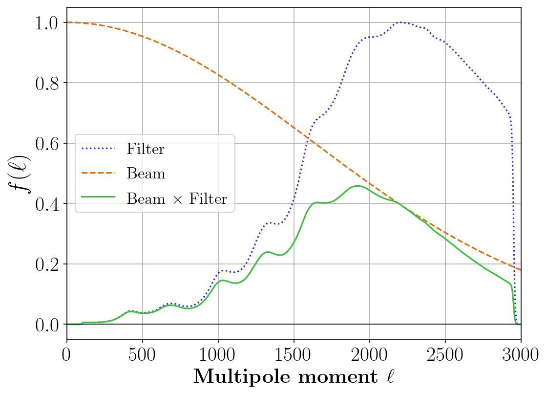
Figure 1: The filter (used to extract the kSZ signal) and beam functions (to account for the finite resolution of the telescope), along with their product versus multipole moment used in the main analysis. See Eqs. 3, 4, and 5 for more details.

A direct cross-correlation of $\Theta^{{\rm kSZ}}$ and $\delta_{g}$ is expected to vanish because of the LOS velocity symmetry of the kSZ signal, which is as likely to be positive as it is to be negative Doré et al. (2004); Hill et al. (2016). Therefore, following the method from Doré et al. (2004); DeDeo et al. (2005); Hill et al. (2016); Ferraro et al. (2016), we first square the filtered kSZ fractional CMB temperature shift $\Theta^{{\rm kSZ}}$ in real space, and then cross-correlate it with the galaxy overdensity $\delta_{g}$ Doré et al. (2004); DeDeo et al. (2005). In the Limber approximation Limber (1957); LoVerde and Afshordi (2008), this yields

$$C_{\ell}^{{\rm kSZ}^{2}\times\delta_{g}}=\frac{1}{c^{2}}\int_{0}^{\eta_{\rm max}}\frac{d\eta}{\eta^{2}}W_{g}(\eta)g^{2}(\eta)\mathcal{T}(k=\frac{\ell}{\eta},\eta),$$ (6)

where $\mathcal{T}(k,\eta)$ is the triangle power spectrum Doré et al. (2004):

$$\mathcal{T}(k,\eta)=\int\frac{d^{2}\bm{q}}{(2\pi^{2})}f(q\eta)f(|\bm{k}+\bm{q}|\eta)B_{\delta_{g}{p_{\bm{\hat{n}}}p_{\bm{\hat{n}}}}}(\bm{k},\bm{q},\bm{-k-q}).$$ (7)

The triangle power spectrum $\mathcal{T}(k,\eta)$ is an integral over the hybrid bispectrum $B_{\delta_{g}{p_{\bm{\hat{n}}}p_{\bm{\hat{n}}}}}$ of one density contrast and two LOS electron momenta, $p_{e}(\hat{\bf n})$. Following previous work Doré et al. (2004); DeDeo et al. (2005); Hill et al. (2016); Ferraro et al. (2016), we approximate the hybrid bispectrum as the product of the velocity dispersion and the non-linear matter bispectrum:

$$B_{\delta_{g}{p_{\bm{\hat{n}}}p_{\bm{\hat{n}}}}}=\frac{1}{3}v_{\mathrm{rms}}^{2}B_{\mathrm{m}}^{\mathrm{NL}}\,.$$ (8)

This approximation is equivalent to the statement that the only strongly non-Gaussian field in the five-point function $\langle\delta{\bf v}\delta{\bf v}\delta\rangle$ is the density fluctuation $\delta$, and thus the only non-zero connected term amongst the Wick contractions of this five-point function is that in Eq. 8. The validity of this approach was first assessed analytically in Ref. DeDeo et al. (2005), who showed that Eq. 8 was indeed the dominant term; this approximation was then confirmed in detail via comparison to cosmological hydrodynamics simulations in F16. Here, we follow Hill et al. (2016); Ferraro et al. (2016) in modeling the non-linear matter bispectrum $B_{\mathrm{m}}^{\mathrm{NL}}$ using a fitting function derived from dark-matter-only $N$-body simulations Gil-Marín et al. (2012). Implicitly, we thus assume that the free electron distribution traces that of the dark matter on the scales probed by our measurements. Appendix D discusses this issue in further detail. We compute the velocity dispersion $v_{\mathrm{rms}}^{2}$ using the Halofit prescription for the non-linear matter power spectrum, which increases the overall signal by $\approx 20$% as compared to a linear-theory calculation. The velocity dispersion is discussed further in Section VII and Appendix D.

We note that the non-linear matter bispectrum (or, more directly relevant here, the galaxy-electron-electron bispectrum) can also be computed within the halo model of LSS. In Appendix D, we outline the main aspects of the halo model computation for the one-halo term, which we compute as a cross-check of the fitting-function-based model on small scales, where it may not be expected to be highly precise, and where uncertainties in the galaxy-halo connection may lead to large uncertainties in the projected-field kSZ signal.

Since the visibility function $g(\eta)\propto f_{b}f_{\rm free}$, we have $C_{\ell}^{{\rm kSZ}^{2}\times\delta_{g}}\propto f_{b}^{2}f_{\rm free}^{2}$ Hill et al. (2016); Ferraro et al. (2016). Thus, the kSZ²-LSS cross-correlation is a direct probe of ionized gas in galaxies, groups, and clusters. Alternatively, on large scales for which $f_{b}$ is expected to be equal to the cosmic baryon abundance and $f_{\rm free}$ is close to unity, the kSZ²-LSS cross-correlation could be used to probe dark energy, neutrino masses, modified gravity, and other novel physics through their effects on the large-scale velocity dispersion in Eq. 8 (e.g., DeDeo et al. (2005)).

II.2 CMB lensing contribution

Gravitational lensing generates non-zero correlations between quadratic combinations of Fourier modes in CMB temperature and polarization maps (see, e.g., Lewis and Challinor (2006) for a review of CMB lensing). To lowest order in the CMB lensing potential $\psi_{\rm CMB}$, the correlation of a squared CMB temperature map with the galaxy overdensity field depends directly on the CMB lensing – galaxy cross-correlation, i.e., $\langle T^{2}g\rangle\propto C_{\ell}^{\psi_{\rm CMB}\delta_{g}}$. Since the Wiener filter in Eq. 3 does not completely remove all primary CMB fluctuations, we must account for the lensing contribution in our analysis — indeed, it turns out to be the largest term in the overall signal. Note that the lensing contribution is proportional to the overall amplitude of the $\delta_{g}$ field, which we will denote $b_{g}$ (the amplitude of the linear galaxy bias), and thus its presence actually allows the degeneracy between $b_{g}$ and $A_{\rm kSZ^{2}}$ in the kSZ signal to be broken in our data analysis (H16).

To lowest order in the lensing potential, the CMB lensing contribution to the squared temperature – galaxy cross-correlation is (F16)

$$\begin{multlined}\Delta C_{\ell}^{T^{2}\times\delta_{g}}\approx-2\frac{\ell\ C_{\ell}^{\psi_{\rm CMB}\delta_{g}}}{(2\pi)^{2}}\int_{0}^{\infty}dL^{\prime}L^{\prime 2}f(L^{\prime})C_{L^{\prime}}^{TT}\\ \int_{0}^{2\pi}d\phi\ f(|\boldsymbol{L^{\prime}}+\boldsymbol{\ell}|)\cos\phi,\end{multlined}\Delta C_{\ell}^{T^{2}\times\delta_{g}}\approx-2\frac{\ell\ C_{\ell}^{\psi_{\rm CMB}\delta_{g}}}{(2\pi)^{2}}\int_{0}^{\infty}dL^{\prime}L^{\prime 2}f(L^{\prime})C_{L^{\prime}}^{TT}\\ \int_{0}^{2\pi}d\phi\ f(|\boldsymbol{L^{\prime}}+\boldsymbol{\ell}|)\cos\phi,$$ (9)

where $C_{\ell}^{\psi_{\rm CMB}\delta_{g}}$ is the cross-power spectrum between the gravitational lensing potential and the galaxy overdensity, $C_{L^{\prime}}^{TT}$ is the unlensed primary CMB temperature power spectrum, $f(\ell)$ is defined in Eq. 4, and $\phi$ is the angle between the 2D wavevectors $\boldsymbol{L^{\prime}}$ and $\boldsymbol{\ell}$. This analytic expression for the lensing contribution was compared to numerical simulations in Refs. Ferraro et al. (2016); Hill et al. (2016) and was found to be extremely accurate (agreement at $<3$% precision up to $\ell=3000$). Note that Eq. 9 neglects the ISW contribution to $T^{2}$, but this is orders of magnitude below the lensing term on the scales in our analysis (F16).

To obtain $C_{\ell}^{{\psi_{\rm CMB}}{\delta_{g}}}$, we start with the lensing convergence $\kappa(\bm{\theta})$, which is a weighted projection of the three-dimensional matter overdensity $\delta_{m}$ along the LOS,

$$\kappa(\bm{\theta})=\int_{0}^{\infty}dzW(z)\delta_{m}(\eta(z)\bm{\theta},z),$$ (10)

where the kernel $W(z)$ indicates the lensing strength at redshift $z$ for sources with a redshift distribution $dn(z_{s})/dz_{s}$. For a flat universe,

$$W(z) = \frac{3}{2}\Omega_{m}H_{0}^{2}\frac{(1+z)}{H(z)}\frac{\eta(z)}{c}\int_{z}^{\infty}dz_{s}\frac{dn}{dz_{s}}\frac{\eta(z_{s})-\eta(z)}{\eta(z_{s})},$$

(11)

where $\Omega_{m}$ is the matter density as a fraction of the critical density at $z=0$, $H(z)$ is the Hubble constant at redshift $z$, with a present-day value $H_{0}$, $c$ is the speed of light, and $z_{s}$ is the source redshift. Note that $\int_{0}^{\infty}dz_{s}dn/dz_{s}=1$.

For CMB lensing, there is only one source plane at the last scattering surface $z_{\star}=1090$. Using $dn(z_{s})/dz_{s}=\delta_{D}(z_{s}-z_{\star})$, where $\delta_{D}$ is the Dirac delta function, the CMB lensing kernel is

$$W^{\kappa_{\rm CMB}}(z) = \frac{3}{2}\Omega_{m}H_{0}^{2}\frac{(1+z)}{H(z)}\frac{\eta(z)}{c}\frac{\eta(z_{\star})-\eta(z)}{\eta(z_{\star})}.$$ (12)

In the expression for the angular galaxy number density field $\delta_{g}$, defined in Eq. 2, we can write the projection kernel $W_{g}(\eta)$ explicitly, and thus obtain

$$\delta_{g}(\bm{\theta})=\int_{0}^{z_{\rm max}}dz\,b(z)\frac{dn}{dz}\delta_{m}(\eta(z)\bm{\theta},z)\,,$$ (13)

where $b(z)$ is the galaxy bias, which we allow to depend on redshift (c.f. Eq. 2), with an overall amplitude $b_{g}$.

We can use these results to obtain the auto- and cross-power spectra of these fields as LOS integrals of the three-dimensional matter power spectrum. In the Limber approximation LoVerde and Afshordi (2008); Limber (1957), the CMB lensing – angular galaxy number density cross-correlation is

$$C_{\ell}^{{\kappa_{\rm CMB}}{\delta_{g}}}=\int_{0}^{\infty}\frac{dz}{c}\frac{H(z)}{\eta^{2}(z)}W^{\kappa_{\rm CMB}}(z)\,b(z)\frac{dn}{dz}P\left(k,z\right),$$ (14)

where $P\left(k,z\right)$ is the matter power spectrum evaluated at wavenumber $k=(\ell+1/2)/\eta(z)$ at redshift $z$. We compute the matter power spectrum with CLASS Blas et al. (2011), using the Halofit fitting function Takahashi et al. (2012) to compute non-linear corrections. Our models for $b(z)\frac{dn}{dz}$ and $\frac{dn}{dz}$ for the unWISE galaxy samples are discussed in Section III.2 (see Fig. 2).

Finally, note that the lensing convergence $\kappa$ is related to the lensing potential $\psi$ by $\kappa(\bm{\theta})=-\nabla^{2}\psi(\bm{\theta})/2$ where $\nabla^{2}$ is the two-dimensional Laplacian on the sky, which yields $\kappa_{\ell}=\ell(\ell+1)\psi_{\ell}/2$ in multipole space. Thus

$$C_{\ell}^{{\psi_{\rm CMB}}{\delta_{g}}}=\frac{2}{\ell(\ell+1)}C_{\ell}^{{\kappa_{\rm CMB}{\delta_{g}}}}\,,$$ (15)

which directly enters Eq. 9.

II.3 Magnification bias contributions

The observed galaxy number density fluctuation field, $\delta_{g}$, is the sum of the contribution from intrinsic (physical) fluctuations in the galaxy number density and the contribution from lensing magnification fluctuations coupling to the galaxy field. The latter contribution due to magnification bias can be non-negligible for galaxy samples with luminosity functions that are steep at the faint end, near the threshold for detection. This is quantified by $s\equiv d\log_{10}N/dm$, the logarithmic slope of the galaxy number counts as a function of apparent magnitude $m$ near the magnitude limit of the survey.

The contribution due to magnification bias in the observed galaxy number density field, $\mu_{g}$, can be written as a LOS integral:

$$\mu_{g}(\bm{\theta})=(5s-2)\int_{0}^{\infty}dzW(z)\delta(\eta(z)\bm{\theta},z)\,,$$ (16)

where $W(z)$ is the lensing kernel defined in Eq. 11. The total observed angular number density fluctuation field is then $\delta_{g}^{\rm obs}=\delta_{g}+\mu_{g}$, where $\delta_{g}$ is given by Eq. 13 and $\mu_{g}$ is given above.

The galaxy magnification bias field has a non-zero correlation with both the CMB lensing field and the kSZ² field. We account for both in our analysis, improving upon Refs. Hill et al. (2016); Ferraro et al. (2016), which neglected these contributions. As will be seen below, the magnification bias contributions are relatively small for the lowest-redshift (blue) sample in our analysis, which is similar to the sample used in Hill et al. (2016); Ferraro et al. (2016); thus, the conclusions of that work are unlikely to be strongly biased due to neglecting these terms. However, for the higher-redshift (green and red) samples that we analyze, the magnification bias terms are large and must be included to obtain unbiased results.

Analogous to Eq. 9, the lowest-order expression for the contribution of the CMB lensing – magnification bias cross-correlation to our measured statistic is

$$\begin{multlined}\Delta C_{\ell}^{T^{2}\times\mu_{g}}\approx-2\frac{\ell\ C_{\ell}^{\psi_{\rm CMB}\mu_{g}}}{(2\pi)^{2}}\int_{0}^{\infty}dL^{\prime}L^{\prime 2}f(L^{\prime})C_{L^{\prime}}^{TT}\\ \int_{0}^{2\pi}d\phi\ f(|\boldsymbol{L^{\prime}}+\boldsymbol{\ell}|)\cos\phi\,.\end{multlined}\Delta C_{\ell}^{T^{2}\times\mu_{g}}\approx-2\frac{\ell\ C_{\ell}^{\psi_{\rm CMB}\mu_{g}}}{(2\pi)^{2}}\int_{0}^{\infty}dL^{\prime}L^{\prime 2}f(L^{\prime})C_{L^{\prime}}^{TT}\\ \int_{0}^{2\pi}d\phi\ f(|\boldsymbol{L^{\prime}}+\boldsymbol{\ell}|)\cos\phi\,.$$ (17)

Analogous to Eq. 14, the cross-power spectrum between the CMB lensing and lensing magnification bias fields is

$$C_{\ell}^{{\kappa_{\rm CMB}}{\mu_{g}}}=(5s-2)\int_{0}^{\infty}\frac{dz}{c}\frac{H(z)}{\eta^{2}(z)}W^{\kappa_{\rm CMB}}(z)W(z)P\left(k,z\right),$$ (18)

where $W(z)$ is the lensing kernel of Eq. (11) and $W^{\kappa_{\rm CMB}}(z)$ is the CMB lensing kernel of Eq. (12).

The magnification bias field also correlates with the squared kSZ signal. Following the same approach used above to obtain Eq. 6, the cross-correlation of $(\Theta^{{{\rm kSZ}}})^{2}$ with the magnification bias field $\mu_{g}$ (Eq. 16) is given by

$$C_{\ell}^{{{\rm kSZ}^{2}}\times{\mu_{g}}}=(5s-2)\frac{1}{c^{2}}\int_{0}^{\eta_{\rm max}}\frac{d\eta}{\eta^{2}}W(\eta)g^{2}(\eta)\tau(k=\frac{\ell}{\eta},\eta)\,.$$ (19)

This kSZ²-magnification bias term is the final component of the theoretical model that we fit to the data, in addition to the terms in Eqs. 6, 9, and 17. Note that Eq. 19 describes the correlation between the (squared) kSZ field and the total matter density field, as traced by lensing — the galaxy bias does not appear. Thus a measurement of this term directly probes the manner in which free electrons trace the underlying matter density field, with no need to model the relation between galaxies and matter.

III Data

III.1 CMB Maps

We use several foreground-cleaned blackbody-component CMB temperature maps in this analysis. The primary map that we focus on, as was used in H16, is the “local-generalized morphological component analysis” (LGMCA) map, which was constructed from WMAP 9-year Bennett et al. (2013) and Planck-PR2 Adam et al. (2016) data. The LGMCA method extracts the blackbody CMB signal (including kSZ and ISW) from other sky components by relying on the sparse distribution of non-CMB foregrounds in the wavelet domain Bobin et al. (2014, 2013, 2014). We note that the tSZ signal is explicitly removed in the LGMCA map using a constraint, by taking advantage of the known frequency spectrum of the tSZ effect. While other foregrounds are not explicitly nulled, the dust contamination in the LGMCA map is minimal, as will be shown below.

We also make use of the Planck “spectral matching independent component analysis” (SMICA) map, which is constructed from a linear combination of the nine pre-processed Planck frequency channels from 30 to 857 GHz Adam et al. (2016); Planck Collaboration et al. (2018b). The SMICA algorithm is quite different from that of LGMCA, and is applied in the harmonic rather than wavelet domain, thus providing a useful test for our results. In addition, we consider the “SMICA-noSZ” map, which is similar to SMICA but imposes an explicit spectral constraint to null the tSZ signal, as described above for the LGMCA map. All of the CMB maps described here have an angular resolution of FWHM = 5 arcmin.

Other CMB maps which we use are the LGMCA noise map Bobin et al. (2013, 2014) (constructed from the half-difference of splits of the Planck and WMAP data) for the null tests (see Section IV), Planck 545 GHz (FWHM = 4.63 arcmin) and 857 GHz maps (FWHM = 4.83 arcmin) (Adam et al., 2016) for the explicit dust removal (cleaning procedure described in Section IV) and dust null tests.

Our analysis employs an “asymmetric” technique to construct the $T^{2}$ field, in which we multiply two different CMB maps, one of which has more robust foreground cleaning but lower S/N, and the other of which has higher S/N but slightly higher foreground contamination. The motivation for doing this is to improve the overall S/N of our measurement — by only using a fully-foreground-nulled map in one “leg” of the $T^{2}$ field, we can decrease the noise penalty associated with this foreground cleaning on our measurement (see, e.g., Sultan Abylkairov et al. (2020) for a recent exploration of such tradeoffs in CMB foreground cleaning). This method remains unbiased due to the fact that the full foreground deprojection — in our case, the tSZ removal — has been applied to one of the $T$ maps, and thus even if it is present in the other $T$ map there will still be zero correlation in the final result. This is analogous to recent developments in foreground-immune CMB lensing reconstruction quadratic estimators, which employ one foreground-deprojected $T$ map and one $T$ map in which only total variance minimization has been applied Madhavacheril and Hill (2018); Darwish et al. (2021). In our fiducial analysis, the LGMCA map serves as the fully-foreground-deprojected $T$ map and the SMICA map serves as the $T$ map with slightly lower noise in the asymmetric combination. We explicitly confirm that this choice increases the S/N of our final kSZ measurements by $\approx 10$%, as compared to using the LGMCA map in both legs of the $T^{2}$ combination.

To optimally extract the kSZ signal from the component-separated CMB maps, we use a Wiener filter (nearly identical to the filter used in H16) $F_{\ell}=C_{\ell}^{{\rm kSZ}}/C_{\ell}^{\rm tot}$. As described in Section II, the numerator, $C_{\ell}^{{\rm kSZ}}$, is the theoretical kSZ power spectrum and the denominator, $C_{\ell}^{\rm tot}$, is set to $C_{\ell}^{\rm LGMCA}$, the auto-power spectrum of our main CMB map (LGMCA). The filter is set to zero for $\ell<100$ (to remove any contribution from the ISW effect) and $\ell>3000$ (to remove the noise-dominated modes), multiplied by a hyperbolic tangent to ensure smoothness at the boundaries, and normalized to a maximum value of unity (at $\ell\approx 2200$). The filter function $F(\ell)$ is shown in Fig. 1. The beam window function of the LGMCA maps $b(\ell)$ is modeled as a Gaussian with FWHM = 5 arcmin, and is also shown on this plot, along with the product of the beam and filter functions, $f(\ell)$ (see Equations 4 and 5). To ensure consistency in the filtered kSZ and lensing signals that enter our estimator, we also filter the SMICA map (and SMICA-noSZ) using the same $F(\ell)$ and beam $b(\ell)$ (the SMICA maps also have FWHM = 5 arcmin).

III.2 Galaxy Catalogs

Our LSS tracer is the unWISE galaxy catalog, which is constructed using data from the Wide-Field Infrared Survey Explorer (WISE) mission, and additionally includes the post-hibernation NEOWISE mission Schlafly et al. (2019); Krolewski et al. (2020). The unWISE catalog provides a sample of more than 500 million galaxies with redshift $0<z<2$ across the full sky, and is the largest full-sky galaxy catalog currently available. It is further divided into 3 subsamples using cuts on infrared galaxy color and magnitude, as detailed below: blue, green, and red at mean redshifts $\approx 0.6,1.1,$ and $1.5$, respectively Krolewski et al. (2020).

The WISE mission mapped the entire sky at 3.4, 4.6, 12, and 22 $\mu$m (W1, W2, W3, and W4) with angular resolution of $6.1^{\prime\prime}$, $6.4^{\prime\prime}$, $6.5^{\prime\prime}$, and $12^{\prime\prime}$, respectively Wright et al. (2010); Krolewski et al. (2020). The unWISE galaxies are selected from the unWISE catalog based on cuts on the W1 and W2 magnitudes. Further, stars are removed by cross-matching the catalog with Gaia; each of the samples is required to be either undetected or not point-like in Gaia Krolewski et al. (2020); Gaia Collaboration et al. (2016, 2018). Table 1 gives a summary of the cuts made to construct the three unWISE subsamples. Their important properties are summarized in Table 2, including redshift distribution (mean redshift $\bar{z}$, and redshift width $\delta_{z}$), number density $\bar{n}$, and faint-end logarithmic slope of the luminosity function $s=d\log_{10}N/dm$. The corresponding average halo masses of the samples, as inferred from their halo biases, are $\sim 1$-$5\times 10^{13}$ $h^{-1}$ $M_{\odot}$ Krolewski et al. (2020). The redshift distribution of the galaxies, $b(z)dn/dz$, obtained for each sample in Ref. Krolewski et al. (2020) from cross-correlation with large-area spectroscopic surveys (BOSS galaxies and quasars and eBOSS quasars) is shown in Fig. 2 (the method is described in detail in Newman (2008); McQuinn and White (2013)). The $dn/dz$ curves in Fig. 2 are obtained by dividing the cross-correlation $b(z)dn/dz$ measured in Krolewski et al. (2020) by the best-fit bias model for each sample ($b(z)=0.8+1.2z$ for blue, $b(z)={\rm max}(1.6z^{2},1)$ for green, and $b(z)={\rm max}(2z^{1.5},1)$ for red) and normalizing Krolewski et al. (2020).

unWISE	W2 $<$	W2 $>$	W1 - W2 $>$ x	W1 - W2 $<$ x
blue	15.5	16.7		$\frac{(17-W2)}{4}+0.3$
green	15.5	16.7	$\frac{(17-W2)}{4}+0.3$	$\frac{(17-W2)}{4}+0.8$
red	15.5	16.2	$\frac{(17-W2)}{4}+0.8$

Table 1: Cuts made on infrared color and magnitude in the WISE data to construct the unWISE catalogs (see Schlafly et al. (2019); Krolewski et al. (2020) for further details).

unWISE	$\bar{z}$	$\delta_{z}$	$\bar{n}$	s
blue	0.6	0.3	3409	0.455
green	1.1	0.4	1846	0.648
red	1.5	0.4	144	0.842

Table 2: Important properties of each unWISE sample: $\bar{z}$, mean of redshift from $dn/dz$, see Section III; $\delta_{z}$, width of the redshift distribution (as measured by matching to objects with photometric redshifts on the COSMOS field (Laigle et al., 2016)); $\bar{n}$, the number density per deg²; and $s$, the faint-end slope of the luminosity function $s=d\log_{10}N/dm$. See Schlafly et al. (2019); Krolewski et al. (2020) for further details.

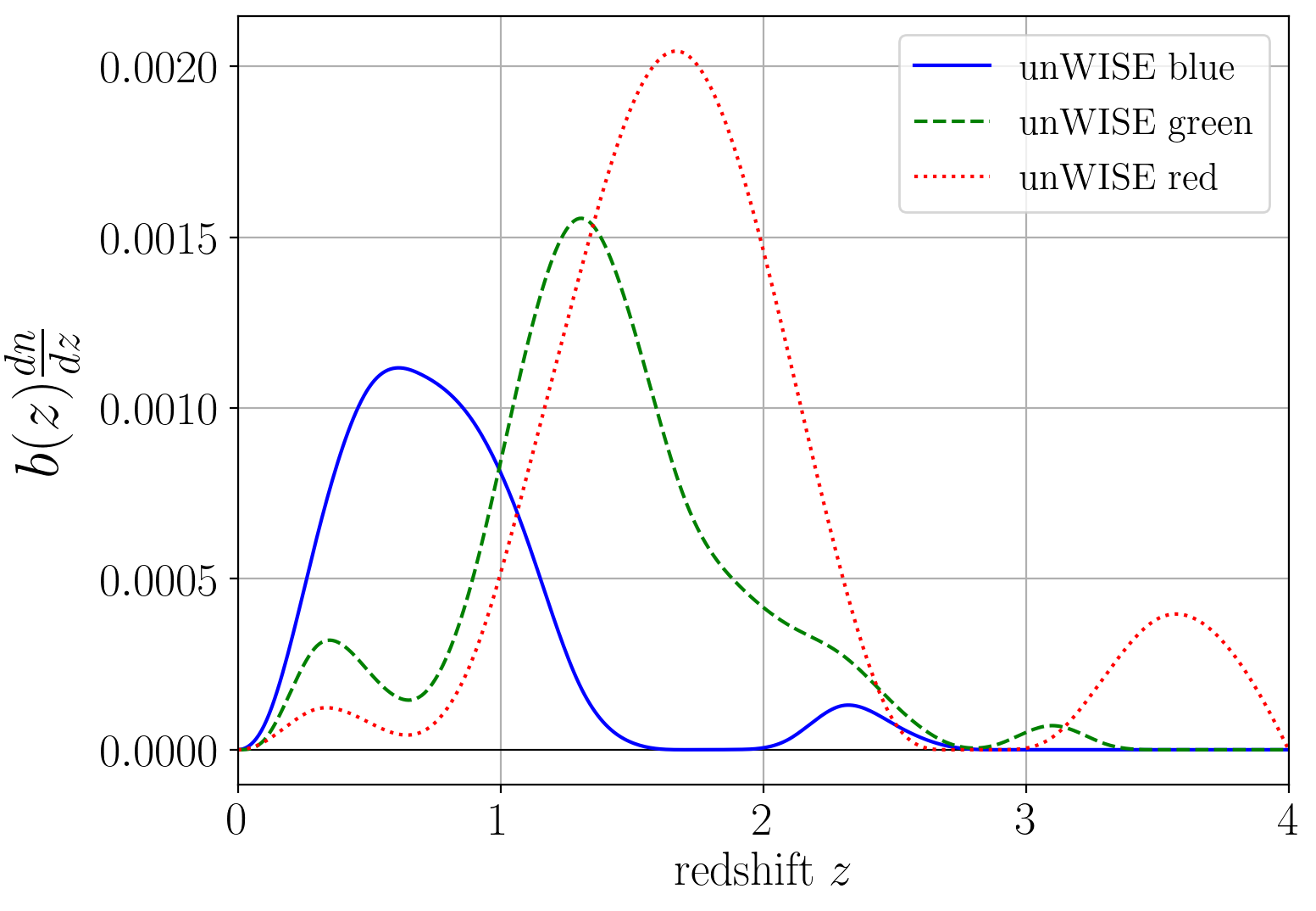
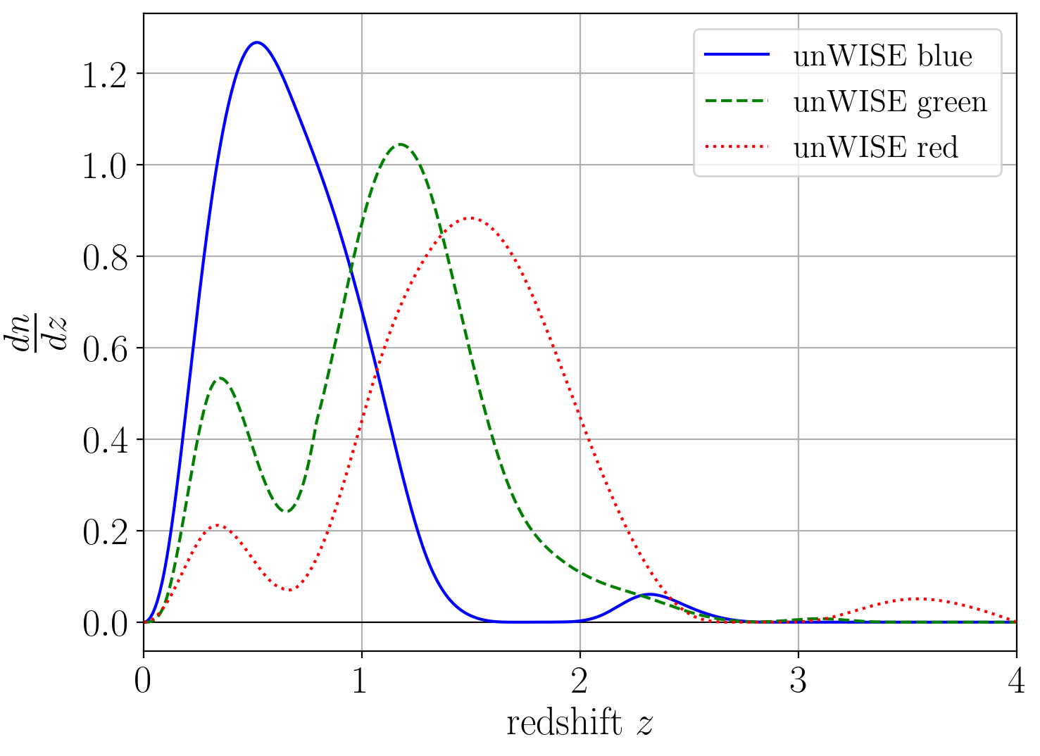
Figure 2: Top: Bias-weighted redshift distributions $b(z)dn/dz$ (obtained by cross-correlation with BOSS and eBOSS surveys) for the blue (solid line), green (dashed line), and red (dotted line) unWISE samples, as measured in (Krolewski et al., 2020). Bottom: Normalized statistical redshift distribution of the unWISE galaxies for the blue (solid line), green (dashed line), and red (dotted line) obtained by dividing the curves from the top panel by a redshift dependent bias $b(z)$ function, and normalizing. See Table 1 for mean redshifts and other properties associated with these galaxy samples.

To remove stellar contamination, we apply a Galactic mask, based on the Planck CMB lensing mask, which also masks point sources, bright stars (cross-matched with CatWISE catalog Eisenhardt et al. (2020)), galaxies (LSLGA catalog), and planetary nebulae, as described in Krolewski et al. (2020). The Planck lensing mask is apodized, while the stellar, large galaxy, planetary nebulae and area-lost masks for the unWISE galaxy map are not, which leaves a sky fraction of $f_{\rm sky}=0.586$.

IV Analysis

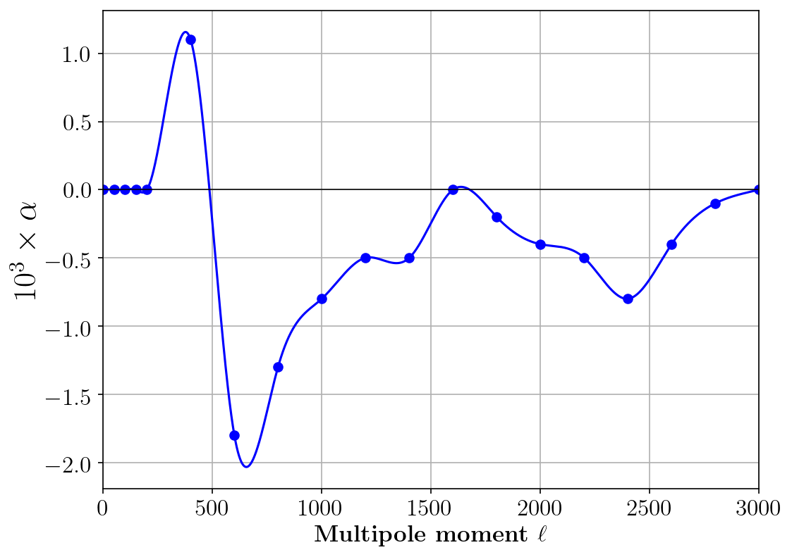
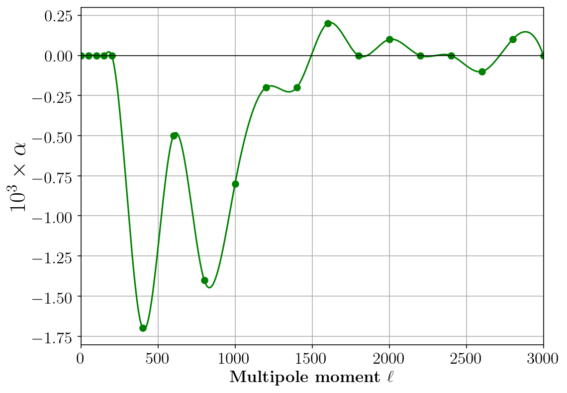
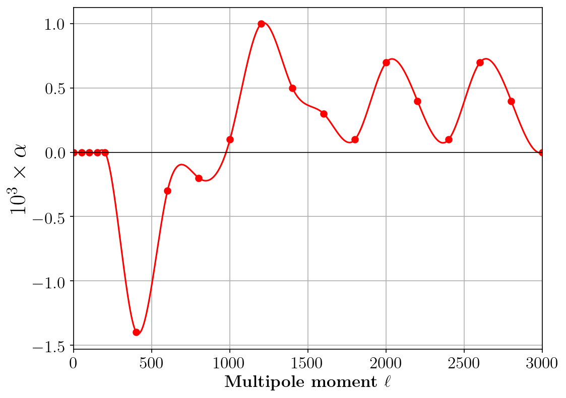
Figure 3: Multipole-dependent $\alpha$ values that null the cross-correlations of $\delta_{g}$ and $((1+\alpha)T_{\rm LGMCA}-\alpha T_{\rm dust})$ for each of the unWISE maps. The $\alpha$ values are found for each of the 13 multipole bins, and then interpolated (using a CubicSpline) over the entire $\ell$ range used in the analysis.

IV.1 Foreground cleaning

Our kSZ²-LSS estimator can potentially be biased by contributions from residual foreground contamination in the cleaned CMB temperature map. As described above, we employ tSZ-deprojected CMB maps (in at least one leg of the estimator), which allows us to robustly avoid any bias from tSZ signal associated with the unWISE galaxies that could have leaked through the component separation process. However, residual thermal dust emission that is present in the CMB maps at the locations of the unWISE galaxies could potentially affect our analysis, since the dust SED is not perfectly known a priori (unlike tSZ), and thus it cannot be exactly removed. Note that our analysis is not biased by residual dust emission in the CMB map that is uncorrelated with the unWISE objects (e.g., from the Milky Way or from galaxies beyond the redshift range of the unWISE samples), but only with residual emission that would be detected by our cross-correlation method.

In order to remove possible unWISE-correlated dust contamination from the LGMCA CMB map that might not have been removed in the original foreground cleaning (Bobin et al., 2013, 2014), we use a cleaning technique similar to the one from H16. We construct a linear combination of the filtered $T_{\rm LGMCA}$ map and a filtered dust map $T_{\rm dust}$ such that it has zero cross-correlation with the unWISE galaxies, i.e., such that any dust associated with the unWISE galaxies is removed. In our analysis, the dust removal procedure is performed bin-by-bin in multipole space. Note that H16 employed a scale-independent cleaning procedure, which we also consider in Appendix A, finding very similar results to those obtained in our scale-dependent approach. Our procedure, which we will often refer to as “$\alpha$-cleaning”, works as follows: for each of the unWISE subsamples, we look for a value $\alpha$ that nulls the cross-correlation of the unWISE galaxy overdensity $\delta_{g}$ and the linear-combination map $((1+\alpha)T_{\rm LGMCA}-\alpha T_{\rm dust})$, where $T_{\rm dust}$ is a map dominated by dust emission (note that our linear combination ensures that even if the dust map contains a small amount of CMB signal, the linear-combination map remains an unbiased CMB map). Our fiducial dust map is the Planck 545 GHz map. We perform this operation independently for each of the 13 linearly-spaced multipole bins from $\ell=300$ to $\ell=2900$ with width $\Delta\ell=200$; we look for an $\ell$-dependent $\alpha_{\rm min}$ that gives exactly null when cross-correlating $\delta_{g}$ and $((1+\alpha)T_{\rm LGMCA}-\alpha T_{\rm dust})$. After determining the $\alpha_{\rm min}$ values for the central $\ell$ value in each bin, we interpolate them over the entire range of multipoles (using the CubicSpline routine). This gives us effectively a smooth $\alpha_{\rm min}$-filter, which we use to construct

$$T_{\rm clean}=(1+\alpha_{\rm min})T_{\rm LGMCA}-\alpha_{\rm min}T_{\rm dust}\,,$$ (20)

where $\alpha_{\rm min}$ is $\ell$-dependent and the operations are performed in harmonic space. The results of this procedure (the $\alpha_{\rm min}$ values and the interpolating function) are shown in Fig. 3.

Even after performing the $\alpha$-based dust cleaning, we want to ensure that our detected $C_{\ell}^{{\rm kSZ}^{2}\times\delta_{g}}$ signal is not due to other effects. When a product of two CMB maps is cross-correlated with a galaxy map, the possible sources of non-zero measurements are: kSZ (our intended signal); tSZ, which we eliminate by always using the tSZ-nulled LGMCA map (or SMICA-noSZ) map in at least one leg of our estimator, such that tSZ will not be picked up in the cross-correlation $(T_{\rm LGMCA}T_{\rm SMICA})\times\delta_{g}^{unWISE}$; CMB lensing contributions, which we account for in our theoretical prediction (see Sections II and V); radio source contamination, which has been tested in H16 to be fully negligible; the dust contribution whose mitigation is described above; and the ISW effect, which we avoid by removing all modes at $\ell<100$ with the filter shown in Fig. 1.

Although we implement the explicit cleaning procedure described above, we apply several tests to ensure the results are not artificial or due to dust contamination, and that our $\alpha$-cleaning was indeed effective. Firstly, we consider cross-correlating the LGMCA noise map ($T_{\rm noise}$) with the unWISE $\delta_{g}$ maps, where one would expect null (Fig. 4 top left). A similar test is done with $T_{\rm noise}^{2}$ (Fig. 4 top right). Both are consistent with null.

The next test we perform is the cross-correlation $(T_{\rm clean}T_{\rm dust})\times\delta_{g}$, which would yield a strong signal if $T_{\rm clean}$ contained even a small amount of unWISE-correlated dust emission, due to the brightness of thermal dust at high frequencies (H16). This particular test is performed twice with two different dust maps: Planck 545 GHz and Planck 857 GHz, where both maps are heavily dust-dominated. In H16, this dust null test was the closest to failing, with probability-to-exceed $p=0.02$ (for 13 degrees of freedom) when fitted to null, although this was dominated by a single data point (H16). Thus it is of interest to see whether our analysis using larger galaxy samples (and hence higher S/N) may see stronger evidence of a failure of this null test, if indeed the $\alpha$-cleaned LGMCA map does contain some residual dust. However, we find that this test is fully consistent with null. Using Planck 545 GHz as $T_{\rm dust}$, we obtain $p=$ 0.46, 0.61, and 0.83 for unWISE blue, green, and red, respectively, for 13 degrees of freedom, when fitting to null. This provides very strong evidence against the presence of dust contamination in our kSZ measurements. The tests (with probabilities-to-exceed $p$) are summarized in Table 3, and shown in Fig. 4.

An additional natural test to perform might seem to be $T_{\rm clean}\times\delta_{g}$. However, since $T_{\rm clean}$ is defined as the linear combination of $T_{\rm LGMCA}$ and $T_{\rm dust}$ that yields zero when cross-correlated with $\delta_{g}$ (see Eq. 20), this test is meaningless as it is guaranteed to pass. Put more simply, the construction of $T_{\rm clean}$ already removes any mean dust residual associated with the unWISE galaxies; the $(T_{\rm clean}T_{\rm dust})\times\delta_{g}$ test is meaningful and informative because it is sensitive to any potential contribution arising from fluctuations in the dust residuals around the zero mean level.

Even though all of our tests show that the dust present in the LGMCA map is effectively negligible, we still want to assess its approximate level, if possible. We do this by measuring $T_{\rm clean}^{2}\times\delta_{g}$ for the unWISE samples and then rescaling the measurements to the primary CMB frequencies using a fiducial thermal dust SED. This procedure is described in detail in Appendix B, and further demonstrates that we can safely assume the dust is not a source of the measured signal in our kSZ analysis.

Moreover, we also ensure that our results are not contaminated by Galactic dust, which could in principle affect the unWISE selection function, and is also present in the mm-wave sky via its thermal emission. Firstly, we note that the CMB maps are filtered to remove the low multipoles (the Wiener filter peaks at $\ell\approx 2000$), where Galactic dust is most important. However, since this is not a stringent test of a potential Galactic dust bias, we re-run our kSZ²-galaxy pipeline (described in detail below in Section IV.2) with a Planck mask with $f_{sky}=0.4$0 combined with the original unWISE mask ($f_{sky}=60$). The results are consistent within the statistical error bars with our fiducial measurements, which indicates that Galactic dust contamination in our measurement is statistically negligible.

unWISE $\times$	$T_{noise}$	$T_{noise}^{2}$	$T_{\rm clean}T_{\rm dust,857}$	$T_{\rm clean}T_{\rm dust,545}$
blue	0.79	0.86	0.83	0.46
green	0.39	0.49	0.72	0.61
red	0.32	1.0	0.95	0.83

Table 3: Testing the dust contamination in the $\alpha$-cleaned LGMCA map. Probability-to-exceed $p$ (for 13 degrees of freedom) for fitting the cross-correlation between the unWISE galaxy maps (blue, green, and red) and the CMB temperature maps ($T_{noise}$, $T_{noise}^{2}$, and $T_{\rm clean}T_{\rm dust}$) to null. $T_{\rm clean}$ is the LGMCA_clean map, $T_{\rm noise}$ is the LGMCA_noise map, and $T_{\rm dust}$ is either the Planck 857 GHz or Planck 545 GHz map.

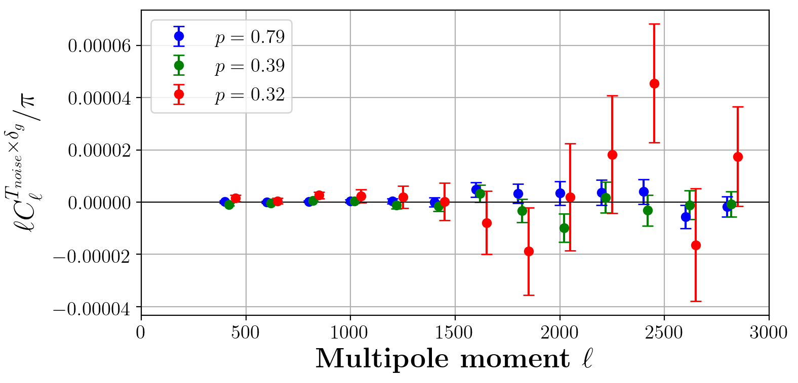
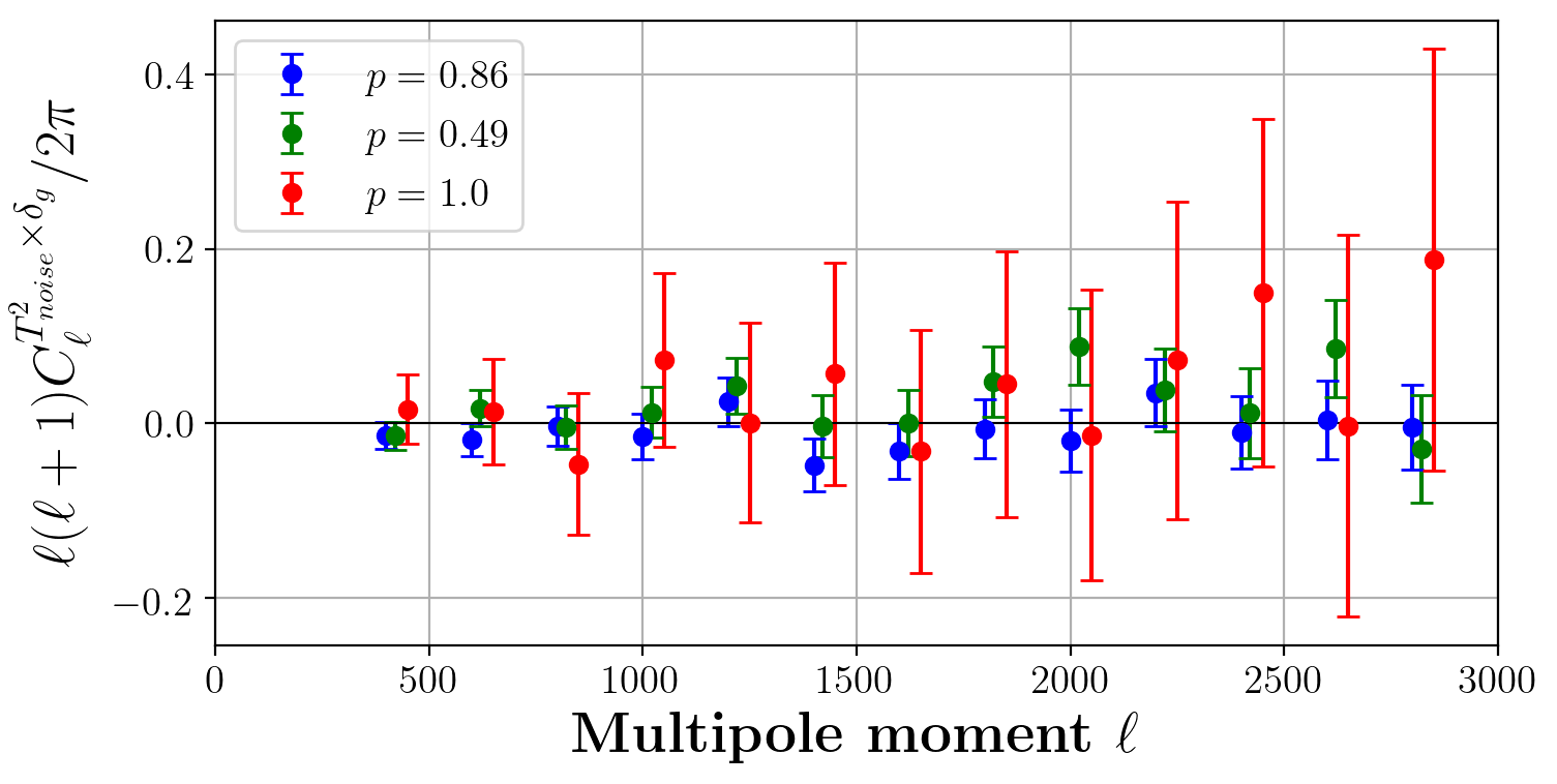
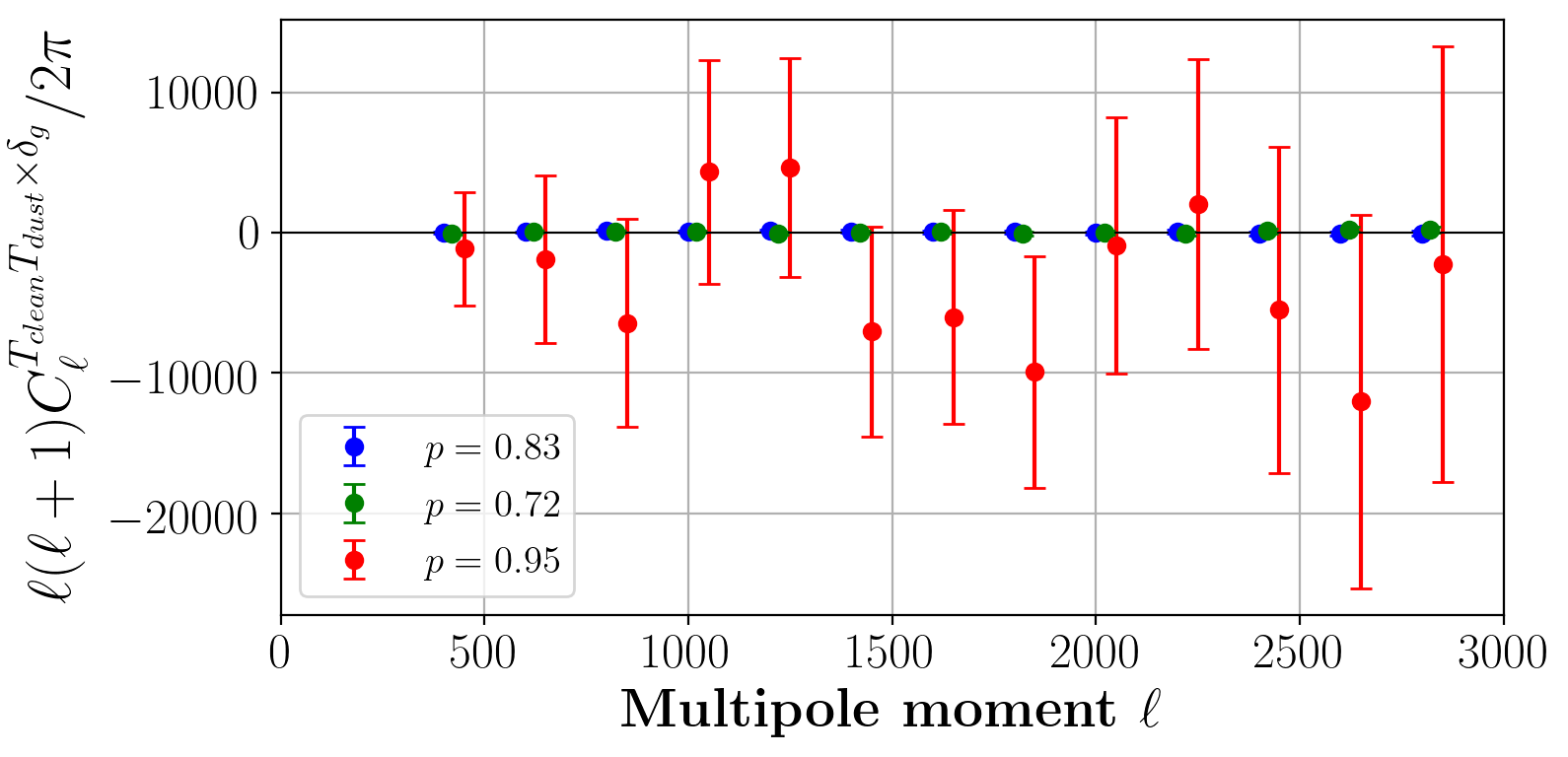
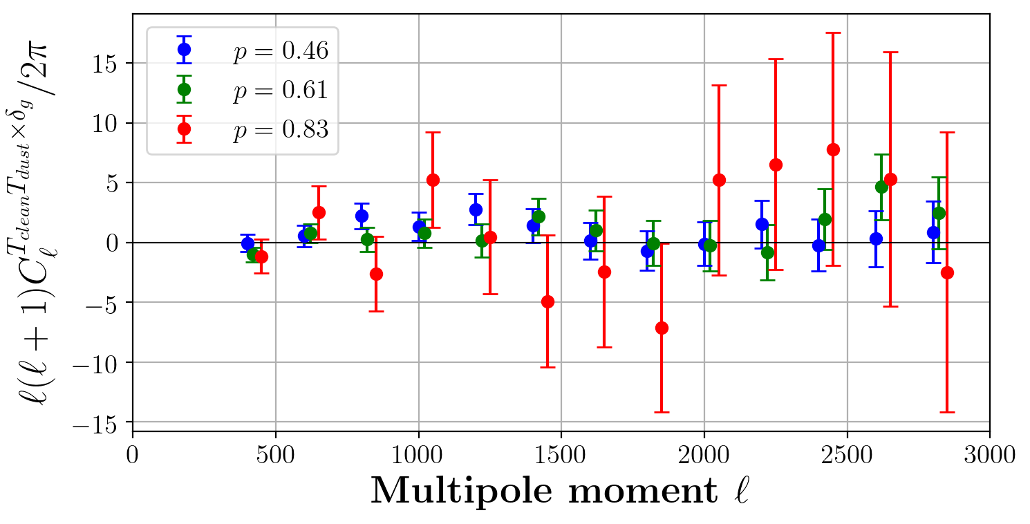
Figure 4: Null tests on the LGMCA maps (noise maps in top panels and the $\alpha$-cleaned maps used in our main data analysis in the bottom panels). All are color coded based on the unWISE colors: blue, red, and green, and include probabilities-to-exceed from fitting them to null. The green points are offset by $\ell=20$, and the red by $\ell=50$ with respect to the true multipole moment values, for visual purposes. Top left: Cross-correlation between $T_{\rm noise}$ and unWISE, where $T_{\rm noise}$ is the LGMCA_noise map. Top right: Cross-correlation between $T_{\rm noise}^{2}$ and unWISE. Bottom left: Cross-correlation of $(T_{\rm clean}T_{\rm dust})$ and unWISE, where $T_{\rm dust}$ is the Planck 857 GHz map. Bottom right: Cross-correlation of $(T_{\rm clean}T_{\rm dust})$ and unWISE, where $T_{\rm dust}$ is the Planck 545 GHz map. All tests are consistent with null, which provides robust evidence that our $\alpha$-cleaned LGMCA map contains negligible thermal dust contamination from the unWISE galaxies.

IV.2 kSZ measurement

Finally, after ensuring that our cleaned CMB map is not contaminated by dust, we can apply the $C_{\ell}^{{\rm kSZ}^{2}\times\delta_{g}}$ estimator to the product of LGMCA_clean and SMICA, and the unWISE $\delta_{g}$, which provides higher S/N than LGMCA${}_{\rm clean}^{2}\times\delta_{g}$ while remaining robust to foregrounds. We multiply the filtered, $\alpha$-cleaned LGMCA map with the filtered SMICA map in real space and cross-correlate the product with each of the masked unWISE galaxy maps, using the Namaster software package Alonso et al. (2019); Senn (2019 (accessed December, 2020). The results are shown in Fig. 5, where we bin the cross-power spectrum signal into 13 multipole bins from $\ell=300$ to $\ell=2900$ with width $\Delta\ell=200$. The covariance matrices of the measurements are estimated in the Gaussian approximation, again using the Namaster code. As expected for a harmonic-space measurement with wide multipole bins, the covariance matrices are close to diagonal, but we use the full covariance matrices in the likelihood analysis in Section V. The error bars shown in all plots are the square root of the diagonal elements of the covariance matrices. We describe the interpretation of these measurements in the next section.

Figure 5: Cross-power spectra of the real-space product of the cleaned, filtered LGMCA map and the filtered SMICA map with each of the unWISE galaxy density maps: blue, green, and red (data points in respective colors). The thin dashed curves show the best-fit CMB lensing contribution (including the lensing-galaxy and lensing-magnification bias terms), the black dotted shows the best-fit kSZ contribution (including the kSZ-galaxy and kSZ-magnification bias terms), and the pink stars show the lensing-subtracted residuals for illustration. The yellow solid curves in each plot show the total best-fit curves, which are the sum of best-fit lensing and best-fit kSZ contributions. The best-fit values for each of the free parameters in the theory model (the kSZ² amplitude $A_{{\rm kSZ}^{2}}$, the galaxy bias $b_{g}$, and the magnification response $s$) are presented in the plot titles. Our fiducial model assumes $A_{{\rm kSZ}^{2}}=1$. The kSZ signal is detected at 1.4$\sigma$, 5.0$\sigma$, and 2.5$\sigma$ significance, respectively, for the three unWISE subsamples.

As a robustness check, we repeat the analysis of the original WISE catalog from H16 using our pipeline (and using the sky mask from that work). We reproduce the results of H16 essentially perfectly, including both the central values and the uncertainties (we find a $\lesssim 10$% difference in the error bar values, which arises from the different cleaning methods used).

V Theoretical interpretation

We fit the measured cross-power spectra using the model described in Section II. The model is a sum of the ${\rm kSZ}^{2}$ signal, $C_{\ell}^{{\rm kSZ}^{2}\times\delta_{g}}$; kSZ magnification bias contribution, $C_{\ell}^{{\rm kSZ}^{2}\times\mu_{g}}$; the CMB gravitational-weak lensing contribution, $C_{\ell}^{T^{2}\times\delta_{g}}$; and the CMB lensing—magnification bias term, $C_{\ell}^{T^{2}\times\mu_{g}}$. We allow a free amplitude for each term: $A_{{\rm kSZ}^{2}}b_{g}$ for the kSZ² term, $A_{{\rm kSZ}^{2}}(5s-2)$ for the kSZ magnification bias, $b_{g}$ for the CMB gravitational lensing, and $(5s-2)$ for the CMB lensing-magnification bias, where $A_{{\rm kSZ}^{2}}$ is the amplitude of the kSZ² signal, $b_{g}$ is the galaxy bias (an overall amplitude of the $\delta_{g}$ field in Eq. 2), and $s$ is the magnification response. The total model is then:

$$\begin{multlined}C_{\ell}^{T^{2}\times\delta_{g}}=A_{{\rm kSZ}^{2}}b_{g}C_{\ell}^{{\rm kSZ}^{2}\times\delta_{g}}+A_{{\rm kSZ}^{2}}(5s-2)C_{\ell}^{{\rm kSZ}^{2}\times\mu_{g}}\\ +b_{g}\Delta C_{\ell}^{T^{2}\times\delta_{g}}+(5s-2)\Delta C_{\ell}^{T^{2}\times\mu_{g}}\end{multlined}C_{\ell}^{T^{2}\times\delta_{g}}=A_{{\rm kSZ}^{2}}b_{g}C_{\ell}^{{\rm kSZ}^{2}\times\delta_{g}}+A_{{\rm kSZ}^{2}}(5s-2)C_{\ell}^{{\rm kSZ}^{2}\times\mu_{g}}\\ +b_{g}\Delta C_{\ell}^{T^{2}\times\delta_{g}}+(5s-2)\Delta C_{\ell}^{T^{2}\times\mu_{g}}$$ (21)

The fiducial model (where the cosmic baryon abundance is taken to be $\Omega_{b}/\Omega_{m}=0.158$) assumes that the kSZ² amplitude is equal to unity, $A_{{\rm kSZ}^{2}}=1$, and is shown in Fig. 6. In these plots, we assume the values derived in Krolewski et al. (2020) for the galaxy bias $b_{g}$ and for the magnification response $s$. They are summarized in Table 4. We note that our model includes the first calculation of the kSZ² $\times$ magnification bias contribution and the CMB lensing $\times$ magnification bias contribution to the $T^{2}\times\delta_{g}$ estimator (these terms were neglected in H16 and F16). For the blue sample, which is most similar to the original WISE sample used in H16 and F16, these terms are negligible, which indicates that the results in those papers were not biased by neglecting these terms. However, for the green and red samples, the magnification bias terms are non-negligible. For the red sample in particular, the fiducial kSZ² $\times$ magnification bias term is nearly equal to the fiducial kSZ² $\times$ galaxy term.

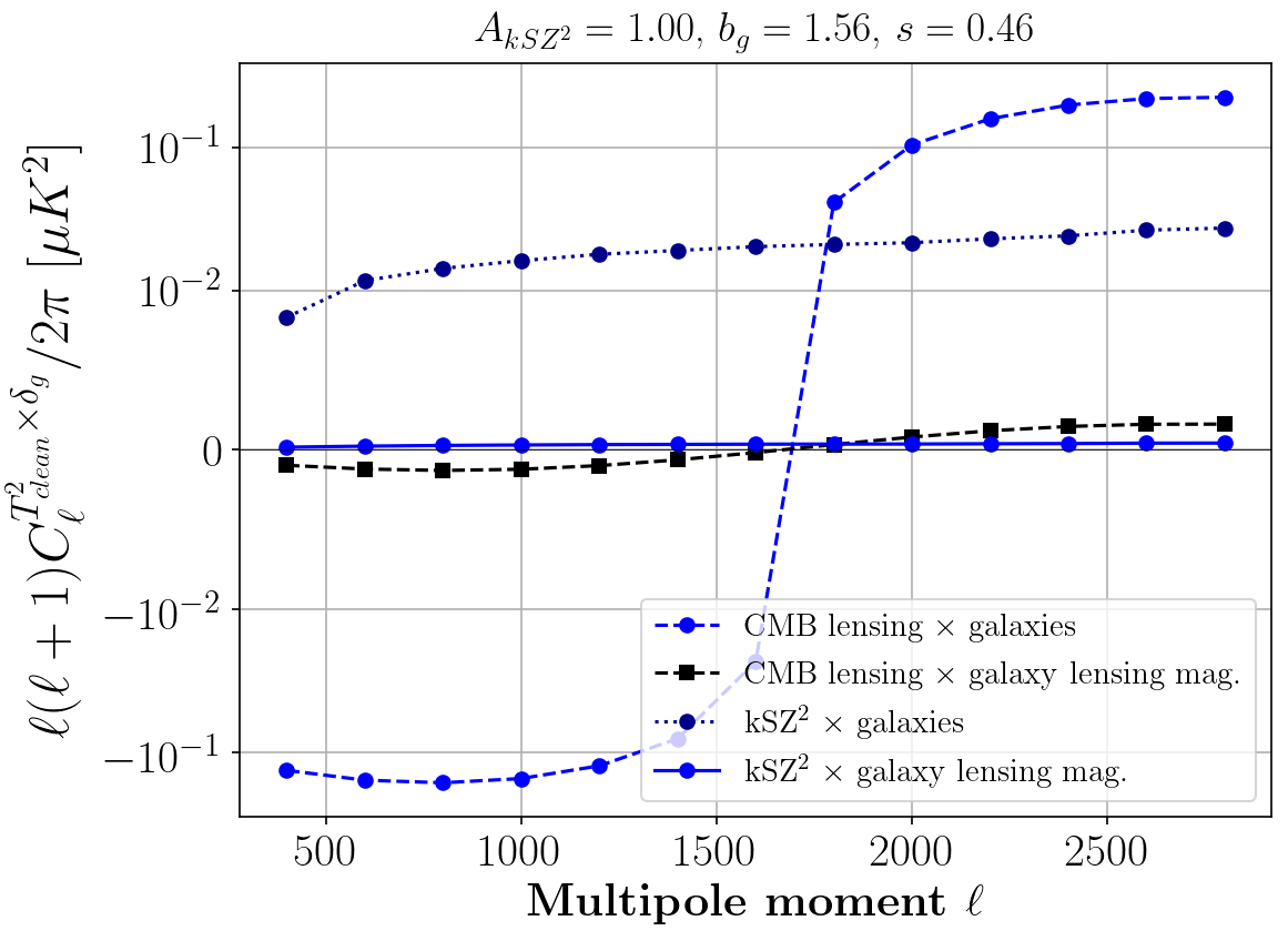
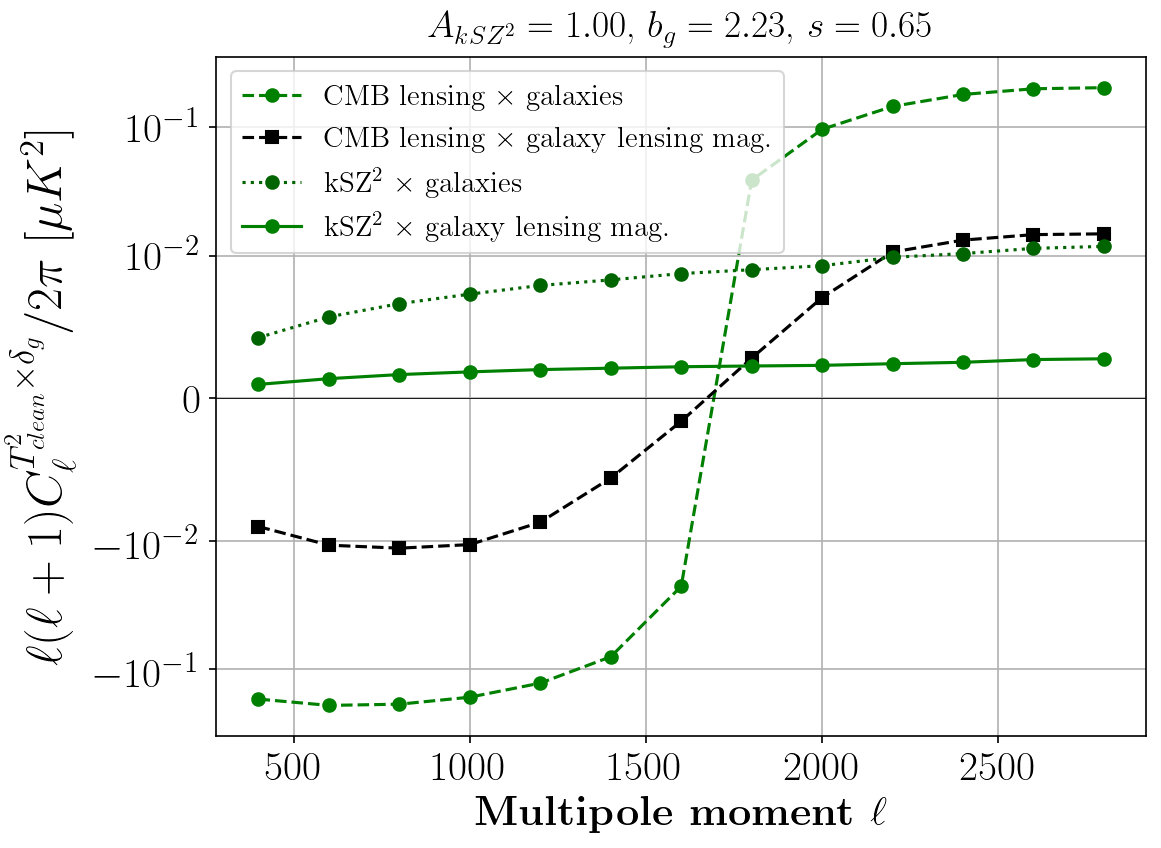
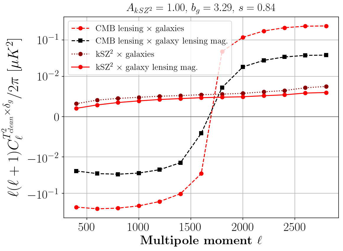
Figure 6: Fiducial model prediction for each of the unWISE samples (color-coded). Each contribution (${\rm kSZ}^{2}$-galaxy cross-correlation, kSZ²-magnification bias cross-correlation, CMB lensing-galaxy cross-correlation, and CMB lensing-magnification bias cross-correlation) is plotted separately. The fiducial model assumes the kSZ² amplitude $A_{{\rm kSZ}^{2}}$ = 1, and the values for the galaxy bias $b_{g}$ and the magnification response $s$ to be equal to the the values measured in Ref. Krolewski et al. (2020). These values are given in the plot titles for ease of reference. The curves are slightly non-smooth because we apply the same binning used in the data analysis to the theory curves here. Note the logarithmic scale on the vertical axis, as compared to the linear scale in Fig. 5.

unWISE	$b_{g}$	$\sigma_{b_{g}}$	$s$	$\sigma_{s}$
blue	1.56	0.0276	0.455	0.046
green	2.23	0.0352	0.648	0.065
red	3.29	0.0352	0.842	0.084

Table 4: Prior values for the galaxy bias $b_{g}$ and the magnification response $s$ for each of the unWISE samples, taken from Krolewski et al. (2020). We take $\sigma_{s}$ to be $0.1s$.

To fit the (LGMCA${}_{\rm clean}\cdot$SMICA) $\times$ unWISE measurements using the theory model in Eq. 21, we assume a multivariate Gaussian likelihood for the data with three free parameters, $A_{{\rm kSZ}^{2}}$, $b_{g}$, and $s$. We adopt a flat prior on $A_{{\rm kSZ}^{2}}>0$, and Gaussian priors on $b_{g}$ and $s$, so that $b_{g}$ is within $1\sigma$ from the values in Table 4 derived in Krolewski et al. (2020), and the prior on $s$ conservatively has 10% width (since the $s$ values are well-determined in Ref. (Krolewski et al., 2020)). The fit is done using the Python Monte Carlo Markov Chain (MCMC) package emcee Foreman-Mackey et al. (2013). The full posterior distributions for the parameters are shown in Appendix C, where we also present an analysis without imposing external priors on $b_{g}$, finding consistent results (with slightly larger error bars).

The best-fit values for $A_{{\rm kSZ}^{2}}$, $b_{g}$, and $s$ obtained from the MCMC procedure, along with the best-fit $\chi^{2}$ values for each unWISE sample are shown in Table 5, and the best-fit theory curves are plotted as yellow solid curves in Fig. 5. The best-fit CMB lensing contribution (the sum of the cross-correlation with both galaxy overdensity and magnification bias) is plotted in dashed unWISE-color-coded curves, and the best-fit kSZ² terms (with the magnification bias term included) are plotted in black dotted curves. Overall we find that the theory model provides a good fit to the data, but with an anomalously high kSZ amplitude for the green subsample. These results are interpreted and discussed further in Section VII.

$unWISE$	$A_{{\rm kSZ}^{2}}$	$b_{g}$	$s$	$\chi^{2}$
blue	0.42 $\pm$ 0.31	1.55 $\pm$ 0.03	0.45 $\pm$ 0.05	10.64
green	5.02 $\pm$ 1.01	2.23 $\pm$ 0.03	0.65 $\pm$ 0.06	11.99
red	8.23 $\pm$ 3.23	3.32 $\pm$ 0.09	0.86 $\pm$ 0.08	11.43

Table 5: Best-fit values for the model parameters (amplitude of the kSZ² signal $A_{{\rm kSZ}^{2}}$, galaxy bias $b_{g}$, and magnification response $s$), obtained by fitting the (LGMCA${}_{\rm clean}\cdot$SMICA) $\times$ unWISE data with the theory model in Eq. 21 for each unWISE sample, along with the minimum $\chi^{2}$ values of the fit (for 10 degrees of freedom).

VI Additional validation

To validate the results for the (LGMCA${}_{\rm clean}\cdot$SMICA) $\times$ unWISE measurement and to ensure they are not artificial or due to foreground contamination, we repeat the analysis with different CMB maps. We consider the following map combinations: (SMICA-noSZ${}_{\rm clean}\cdot$SMICA) $\times$ unWISE; LGMCA${}_{\rm clean}^{2}$ $\times$ unWISE; and SMICA-noSZ${}_{\rm clean}^{2}$ $\times$ unWISE. In all cases, we utilize at least one map that is fully tSZ-deprojected and has been cleaned with the $\alpha$-cleaning procedure described in Sec. IV, which ensures robustness against both tSZ and dust foregrounds. The results of all analyses agree with those of our main analysis presented earlier, (LGMCA${}_{\rm clean}\cdot$SMICA) $\times$ unWISE, and with each other within the uncertainties (see Figs. 17 and 18). As a further test, we also consider the cross-power spectrum of SMICA${}_{\rm clean}^{2}$ with unWISE, which in principle contains a non-zero bias from tSZ residuals in the SMICA map (since it is not a tSZ-deprojected map); nevertheless, we find that it gives fairly close results to those from our main analysis, indicating that any tSZ bias was already quite small, even before tSZ deprojection was applied in the LGMCA and SMICA-noSZ maps.

We briefly describe each of these analyses in the following subsections. The associated plots can be found in Appendix E.

VI.1 (SMICA-noSZ$\cdot$SMICA) $\times$ unWISE analysis

Firstly, we consider an analysis using the Planck SMICA-noSZ map as the main CMB map instead of the LGMCA map. Like LGMCA, the SMICA-noSZ map includes tSZ deprojection in the component separation process, ensuring no tSZ residuals are present in this map. The SMICA-noSZ map is $\alpha$-cleaned, filtered, multiplied in real space with the original SMICA map, and the product is then cross-correlated with each of the unWISE samples. The $\ell$-dependent $\alpha$-cleaning procedure for SMICA-noSZ is performed with the Planck 545 GHz dust map. We also apply the dust null tests described in Section IV.1 on the clean SMICA-noSZ map with both the Planck 545 GHz and 857 GHz dust maps (Fig. 13). They are both consistent with null, showing no evidence of bias.

The (SMICA-noSZ${}_{\rm clean}\cdot SMICA)$ $\times$ unWISE measurements (Fig. 14) are then fit with the same theory model as in the main analysis. The results are very similar to those of our fiducial analysis in Section V, which ensures that the main results are not artificial. Again, the theory model describes the data well, but the inferred value of $A_{{\rm kSZ}^{2}}$ for the green sample is anomalously high.

VI.2 LGMCA${}^{2}\times$ unWISE analysis

The analysis is also conducted as in H16, where we simply square the filtered, $\alpha$-cleaned LGMCA map (the same map used as the first leg of the estimator in our main analysis), and then cross-correlate it with each of the unWISE samples. The results are shown in Fig. 15 in the Appendix E. They are consistent with those of our main analysis, which further validates our measurements. Also, the comparison of these LGMCA${}_{\rm clean}^{2}$ results with our “asymmetric” (LGMCA${}_{\rm clean}\cdot$ SMICA) results clearly demonstrates that the asymmetric approach is not biased by dust (despite only cleaning one leg of the estimator), as expected due to its construction.

VI.3 SMICA-noSZ${}^{2}\times$ unWISE analysis

We also conduct a similar analysis for the SMICA-noSZ map. We square the filtered, $\alpha$-cleaned SMICA-noSZ map, and then cross-correlate it with the unWISE samples. The results are shown in in the Appendix in Fig. 16, and they are again consistent with our fiducial analysis and with those in the previous subsections. This analysis thus also further validates our results.

VI.4 Comparison of the different combinations

A comparison of the results of all combinations is shown in Figs. 17 (SMICA-noSZ) and 18 (LGMCA), along with the cross-correlation of the original SMICA map (filtered, $\alpha$-cleaned, and squared) with the unWISE data. SMICA-noSZ or LGMCA in these plots are the clean maps (using the $\alpha$-cleaning procedure).

The original SMICA map, in contrast to SMICA-noSZ or LGMCA, includes residuals due to tSZ contamination, which can bias our estimator; this is why we do not use it as the primary map in our analysis. However, for the same reason, the SMICA map also has lower noise than SMICA-noSZ or LGMCA, as the explicit deprojection of the tSZ signal in the latter maps leads to the loss of a degree of freedom in the variance-minimization procedures used in component separation. This is why it is advantageous for us to build the asymmetric combination (LGMCA${}_{\rm clean}\cdot$SMICA) or (SMICA-noSZ${}_{\rm clean}\cdot$SMICA), which have lower noise than LGMCA${}_{\rm clean}^{2}$ or SMICA-noSZ${}_{\rm clean}^{2}$, respectively. Moreover, these asymmetric combinations remain robust against tSZ contamination because the tSZ signal is explicitly nulled in the first leg of the combination (LGMCA or SMICA-noSZ).

The primary takeaway from Figs. 17 and 18 is that all of the measurements agree within the statistical uncertainties. However, it is also noticeable that the SMICA${}^{2}\times$ unWISE points show some differences compared to the other measurements, which is very likely due to the tSZ residuals in the SMICA map. This justifies the need for our use of the LGMCA or SMICA-noSZ maps as the primary map in our analysis. Overall, the consistency of the measured cross-correlation of the unWISE maps with all of the quadratic combinations considered here, including (LGMCA${}_{\rm clean}\cdot$SMICA), (SMICA-noSZ${}_{\rm clean}\cdot$SMICA), LGMCA${}_{\rm clean}^{2}$, and SMICA-noSZ${}_{\rm clean}^{2}$, clearly demonstrates the robustness of our measurements.

VI.5 Shifting the Redshift Distribution

We also test the impact of varying the unWISE redshift distributions on our final results. As shown in Fig. 2, we use both the redshift distributions $dn/dz$ and bias-weighted redshift distributions $b(z)dn/dz$ for each sample to obtain the theory components in our model. Note that $dn/dz$ is used to compute the kSZ²-galaxy and lensing-galaxy theory terms, while $b(z)dn/dz$ is used in the kSZ²-magnification and lensing-magnification terms. The bias-weighted redshift distributions are obtained by cross-correlating the unWISE catalogs with the spectroscopic BOSS and eBOSS surveys. The redshift distributions $dn/dz$ are on the other hand obtained by dividing $b(z)dn/dz$ by the redshift-dependent bias functions $b(z)$ for each sample (see Krolewski et al. (2020) for more details). Since the $b(z)dn/dz$ are known to a better precision than $dn/dz$, we consider a 3% shift in the bias-weighted distribution and a 10% shift in $dn/dz$. We emphasize that these should be viewed as fairly extreme shifts, particularly in $b(z)dn/dz$.

We then re-run our parameter inference pipeline for these shifted theoretical templates. The shift changes the amplitude of the kSZ signal $A_{kSZ^{2}}$ for the blue sample to $0.38\pm 0.28$, for the green sample to $4.05\pm 0.93$, and for the red sample to $7.09\pm 3.10$. Even though these values are within the statistical error bars of our original results, and the considered case is quite extreme, the shift in $A_{kSZ^{2}}$ is non-negligible. Thus, we use the results obtained from shifting $dn/dz$ and $b(z)dn/dz$ to estimate the associated systematic error in our final quoted results. We consider the shift in the central values to represent a $2\sigma$ systematic error (as the shifted templates are quite extreme), and thus quote half of these shifts as a representative $1\sigma$ systematic error.

VII Discussion and Future Directions

Our measurements are well-described by the model in Eq. 21. From the best-fit $\chi^{2}$ values, for 10 degrees of freedom, the probabilities-to-exceed are $p=$ 0.39, 0.29, and 0.33 for the blue, green, and red samples, respectively. These galaxies have average halo masses $\sim 1$-$5\times 10^{13}$ $h^{-1}M_{\odot}$ Krolewski et al. (2020).

The measured kSZ² amplitudes, $A_{{\rm kSZ}^{2}}$, are $=0.42\pm 0.31$, $5.02\pm 1.01$, and $8.23\pm 3.23$ for the cross-correlation with the unWISE blue, green, and red samples, respectively. Including the systematic error from shifting the $dn/dz$ and $b(z)dn/dz$ distributions (see Subsection VI.5), the results are $A_{\rm kSZ^{2}}=0.42\pm 0.31\,(stat.)\pm 0.02\,(sys.)$, $5.02\pm 1.01\,(stat.)\pm 0.49\,(sys.)$, and $8.23\pm 3.23\,(stat.)\pm 0.57\,(sys.)$. To our knowledge, these are the highest-redshift kSZ measurements to date. Including both the statistical and systematic errors, these results are within 1.9$\sigma$, 3.6$\sigma$, and 2.2$\sigma$ of our fiducial model, respectively, for which $A_{{\rm kSZ}^{2}}=1$ (Fig. 6). We discuss the tension between our fiducial model and the inferred kSZ amplitude for the green sample in detail below.

The statistical significance of our $A_{{\rm kSZ}^{2}}$ detections for the blue, green, and red samples are 1.4$\sigma$, 5.0$\sigma$, and 2.5$\sigma$, respectively. If the measurements were all uncorrelated, the overall detection significance would be $5.8\sigma$; however, since the samples have non-negligible overlap in redshift (see Fig. 2) and we use the same CMB data in all three measurements (hence with the same noise), the measurements will be somewhat correlated. It is beyond the scope of our current analysis to estimate the covariance of the three measurements; however, it is clear that the correlation will not be 100%, and thus the overall detection significance of the kSZ signal across the three samples is greater than 5$\sigma$. Our measurement is the most sensitive to date of the kSZ signal using the kSZ²-LSS estimator.

Using the inferred kSZ amplitudes, we can constrain the product of the fraction of baryonic matter $f_{b}$ and the fraction of free electrons $f_{\rm free}$ for each unWISE sample. We find $f_{\rm free}$ to be $(f_{b}/0.158)(f_{\rm free}/1.0)=0.65\pm$ $0.24$, $2.24\pm$ $0.25$, and $2.87\pm$ $0.57$ at redshifts $z\approx$ 0.6, 1.1, and 1.5, respectively. At these redshifts, we expect $f_{\rm free}\approx 0.8-0.9$, since all baryons are in an ionized form except for the fraction locked up in stars or the small pockets of neutral hydrogen gas. Thus, as found in H16, our measurements confirm that the expected abundance of baryons based on BBN and primary CMB measurements is indeed present at these redshifts (i.e., there are no “missing baryons” on the relatively large scales probed by our data).

While the data are well-described by the theory model, and the blue and red $A_{{\rm kSZ}^{2}}$ values are within 1.9$\sigma$ and 2.2$\sigma$ of the fiducial prediction, the green $A_{{\rm kSZ}^{2}}$ is anomalously high. As we have robustly verified that our measurements are not contaminated by dust (see Sections IV and VI and Appendices A and B), we consider other possible explanations for the high $A_{{\rm kSZ}^{2}}$ amplitude of the green sample. Here, we emphasize that the detection significance of the kSZ signal in our measurements would not be affected by a change in the theoretical model that solely rescales the signal by an overall factor (as the best-fit $A_{\rm kSZ^{2}}$ value and its error bar would both be changed by the same factor).

First, we note that our fiducial theoretical model may be less accurate on small scales, particularly at high redshifts, as it relies on a fitting function for the non-linear matter bispectrum that is calibrated from $N$-body simulations (see Section II), which may begin to break down in these regimes. It also assumes that the full signal simply scales as the linear galaxy bias, which is expected to break down on small scales where the one-halo term dominates. To investigate these assumptions, we perform a first calculation of the one-halo term for the kSZ²-LSS estimator in Appendix D. We generally find consistency with the fitting function-based model, although the halo model calculation makes clear that the signal depends strongly on the assumed shape of the electron distribution on small scales (where our fiducial calculation assumes it to trace the dark matter) — see Fig. 12. In future work, a full halo model will be used to interpret the measurements presented in this paper and derive constraints on the shape and amplitude of the electron profiles of the unWISE galaxies.

As a further test of potential issues with our model on small scales, we consider fitting the cross-power spectra as a function of $\ell_{\rm max}$ (in our fiducial analysis we have $\ell_{\rm max}=2900$). Since the one-halo term is only significant at high $\ell$ (small scales), we would expect the kSZ² amplitude $A_{{\rm kSZ}^{2}}$ to approach our fiducial model value of unity as we decrease the maximum value of $\ell$, if indeed our model for the small-scale signal is inaccurate. The trend that we observe is qualitatively consistent with this expectation, although the changes in $A_{\rm kSZ^{2}}$ are not dramatic, and the error bars on $A_{\rm kSZ^{2}}$ are somewhat too large to draw a firm conclusion. As an example, for the green sample, when including only the first seven data points ($\ell_{\rm max}=1700$), we obtain $A_{\rm kSZ^{2}}=4.82\pm 1.19$, and for the first five data points ($\ell_{\rm max}=1300$) $A_{\rm kSZ^{2}}=4.52\pm 1.31$. This may be some evidence that a more accurate model of the one-halo term could explain our high green $A_{{\rm kSZ}^{2}}$ measurement, but the trend is only suggestive at present, as these shifts are $<1\sigma$.

Second, in our model we make the assumption that the hybrid bispectrum (Eq. 8) can be factored into the product of the 3D velocity dispersion $v_{\rm rms}$ (computed with the Halofit non-linear prescription) and the non-linear matter bispectrum $B^{\rm NL}_{m}$. Our calculation of $v_{\rm rms}$ is a slight modification of that in H16 and F16, in which linear theory was used; the inclusion of non-linear power increases the predicted kSZ signal by roughly 20%. Additional refinement of the non-linear corrections is unlikely to change this value significantly, as the rms velocity is dominated by linear fluctuations. However, on small scales we might expect the presence of highly non-perturbative effects due to galaxy formation physics, such as velocity outflows in the ionized gas driven by feedback events (e.g., accretion onto supermassive black holes). Recent analyses of the Illustris-TNG simulations indicate that these outflows can reach velocities up to $\approx 2000$ km/s (i.e., several times larger than $v_{\rm rms}$) out to scales as large as 300 kpc Nelson et al. (2019); Pillepich et al. (2019). Moreover, these outflows are expected to be larger at higher redshifts Nelson et al. (2019), which is consistent with the trend in our results from the low-redshift blue sample to the progressively higher-redshift green and red samples. Since our measured cross-power spectrum is an integral over the full bispectrum that is particularly sensitive to squeezed triangles (see Eq. 23), seemingly small-scale effects like gas outflows can change the signal on surprisingly large scales. Thus, our measurements could be an intriguing sign of feedback activity at high redshifts. In this case, the use of perturbation theory to approximate the hybrid bispectrum would be invalid, and a model of the outflow velocities would be needed to interpret the signal. We plan to explore this possibility using hydrodynamical simulations in future work.

In conclusion, the excess signal in one of the unWISE samples can potentially be explained by physical effects that have not been accounted for in our analysis, and we have robustly shown that it is not due to foreground contamination. We will investigate these explanations in detail in future work using the halo model and hydrodynamical simulations.

The future of measurements with the kSZ²-LSS estimator is bright. As shown in F16, the S/N of this estimator grows rapidly as smaller scales can be probed, which is now possible with multifrequency high-resolution CMB maps from ACT Aiola et al. (2020); Naess et al. (2020) and the South Pole Telescope Benson et al. (2014), as well as future maps from the Simons Observatory Ade et al. (2019) and CMB-S4 Abazajian et al. (2019). Upcoming data will yield kSZ detections with S/N an order of magnitude (or more) higher than that found here (see forecasts in F16). Crucial to this approach, however, will be the construction of robust component-separated blackbody CMB temperature maps from high-resolution ground-based data (see Madhavacheril et al. (2020) for a first effort in this direction). Moreover, in our analysis, we have considered galaxies as tracers of the matter overdensity field, but the method can be extended to other tracers, including quasars, weak lensing shear maps, or 21 cm fluctuations Doré et al. (2004); DeDeo et al. (2005); Ma et al. (2018); La Plante et al. (2020).

Appendix A Constant $\alpha$ cleaning for LGMCA

To remove possible unWISE-correlated dust contamination from the LGMCA map, we use the $\ell$-dependent $\alpha$ cleaning technique, which is described in detail in Section IV. However, this procedure can also be done for a constant (not $\ell$-dependent) $\alpha$. As before, we cross-correlate the unWISE galaxy overdensity $\delta_{g}$ with $((1+\alpha)T_{\rm LGMCA}-\alpha T_{\rm dust})$, where $T_{\rm dust}$ is a dust-dominated map; as in the main analysis, we use the Planck 545 GHz map as our fiducial choice. Now, we look for an $\alpha_{\rm min}$ which minimizes the $\chi^{2}$ when fitting all 13 binned $D_{\ell}$ values to null (in the main analysis, we look for an $\alpha_{\rm min}$ which is closest to zero when cross-correlating $\delta_{g}$ with $((1+\alpha)T_{\rm LGMCA}-\alpha T_{\rm dust})$ in each bin separately, and then interpolate these $\alpha$ values within the range $\ell=300$ to $\ell=2900$). In the scale-independent approach here, we find the $\alpha_{\rm min}$ values are -0.00040 $\pm$ 0.00001, -0.00007 $\pm$ 0.00001, 0.00037 $\pm$ 0.00001 for unWISE blue, green, and red, respectively. Then, a new map $T_{\rm clean}=(1+\alpha_{\rm min})T_{\rm LGMCA}-\alpha_{\rm min}T_{\rm dust}$ is constructed separately for each of the unWISE maps, as in Eq. 20, but now with a trivial scale-independent operation instead of a multipole-dependent operation.

As in Section IV, we perform null tests ($T_{\rm clean}\times\delta_{g}$, $T_{\rm clean}T_{\rm dust}\times\delta_{g}$,) with the $T_{\rm clean}$ maps. The constant $\alpha$-cleaning results are summarized below; Fig. 7 and Table 6 show the null tests performed, along with the probabilities-to-exceed for each test and unWISE color in the table. Note that we do not perform the $T_{noise}$ and $T_{noise}^{2}$ tests since the LGMCA noise map does not change here.

In the analysis in H16 (where the constant $\alpha$-cleaning method was also used), the dust null test $(T_{\rm clean}T_{\rm dust})\times\delta_{g}$ was only marginally consistent with null, with $p=0.02$. However, we find that it is consistent with null ($p=$ 0.45, 0.62, and 0.82 for unWISE blue, green, and red, respectively) for the constant-$\alpha$ cleaning here, as for the $\ell$-dependent $\alpha$-cleaning in Section IV. However, the null test is marginal for the cross-correlation between the unWISE green sample and $T_{\rm clean}$, with $p=0.03$. This test is semi-meaningful here since the nulling procedure to determine $\alpha$ is not done $\ell$-by-$\ell$, but rather for all bins simultaneously. We take this as a clear sign that the $\ell$-dependent approach used in our main analysis is preferable due to its robust ability to handle residuals that have non-negligible changes in sign (which are responsible for the marginal issue here — see the green points in Fig. 7 left panel).

Overall we conclude that both $\alpha$-cleaning approaches (scale-dependent or scale-independent) yield maps with no evidence of unWISE-correlated dust contamination, but we adopt the $\ell$-dependent cleaning approach in our main analysis due to its greater robustness.

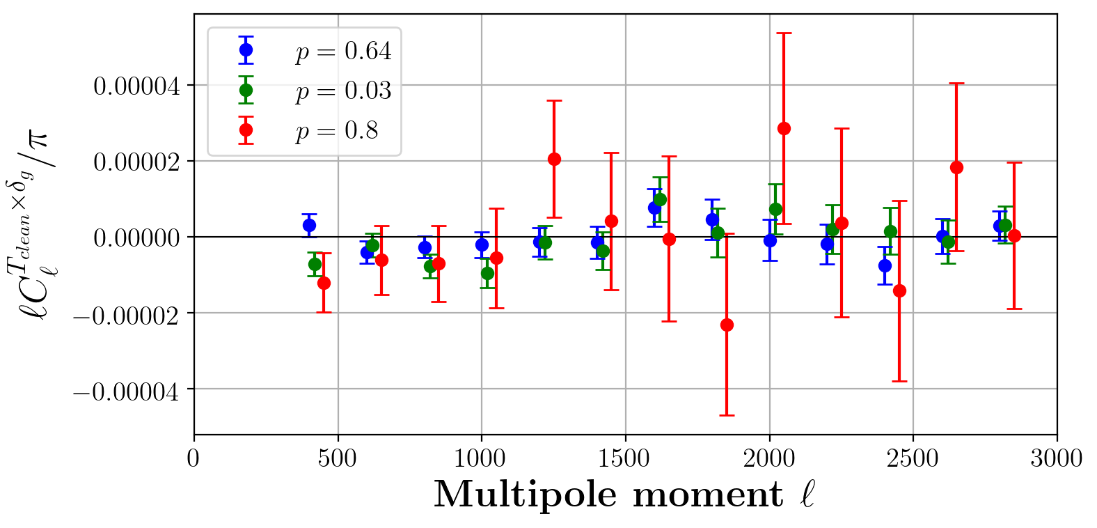
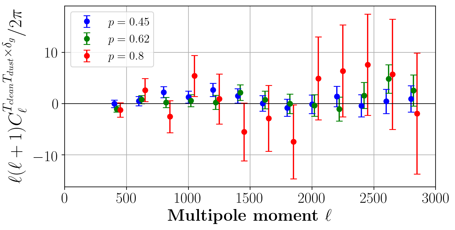
Figure 7: Null tests on the LGMCA_clean map for the constant $\alpha$ cleaning. Both plots are color coded based on the unWISE colors: blue, red, and green, and include their respective $p$-values (for 13 degrees of freedom) in the legend when fitting them to null. Green is offset by $\ell=20$, and red by $\ell=50$ with respect to the true multipole moment values, for visual purposes. Left: Cross-correlation between $T_{\rm clean}$ and unWISE. Right: Cross-correlation between $T_{\rm clean}T_{\rm dust}$ and unWISE, where $T_{\rm dust}$ is Planck 545 GHz map.

unWISE $\times$	$T_{\rm clean}$	$T_{\rm clean}T_{\rm dust}$
blue	0.64	0.45
green	0.03	0.62
red	0.80	0.80

Table 6: Cross-correlation between the unWISE galaxy maps (blue, green and red), and the CMB temperature maps ($T_{\rm clean}$, $T_{\rm clean}T_{\rm dust}$) with probabilities-to-exceed (for 13 degrees of freedom) to test the dust contamination, where $T_{\rm dust}$ is Planck 545 GHz map, and $T_{\rm clean}$ is the LGMCA_clean map, cleaned using the constant $\alpha$ method.

Appendix B Dust assessment in the LGMCA map

Although we performed foreground cleaning and found no evidence of bias, we decided to further investigate the possible dust contamination in the LGMCA map, and assess its level. To estimate the amount of dust in this CMB map, we cross-correlate the squared Planck 545 GHz with unWISE, and then rescale it down to the Planck 143 GHz frequency. The Planck 545 GHz map is dominated by dust, so it is justified to neglect any other components at this particular frequency channel. Then, however, we have to rescale this measurement down to the lower frequencies that dominate our LGMCA kSZ measurement, i.e., to 143 GHz. Using a standard modified blackbody dust SED (e.g., Eq. 6 in Madhavacheril et al. (2020)) with temperature $T_{\rm dust}$ = 24 K and spectral index $\beta$ = 1.40, 1.33, 1.27 for the blue, green, and red samples, respectively, we find the rescaling factor from 545 GHz to 143 GHz to be 328.5 for maps in CMB temperature units, and from 545 GHz to 217 GHz to be 116.6. As a test of this rescaling factor, we measure the ratio of Planck 545 GHz $\times unWISE$ to Planck 217 GHz $\times unWISE$ measurements, both of which are dust-dominated (since the tSZ signal vanishes at 217 GHz). This gives a ratio in the range of 115-120 for our $\ell$ range (which avoids any ISW contributions), which validates the SED rescaling model that we adopt.

In this dust assessment, we want to include an “additional cleaning factor” that approximately captures how much the original LGMCA cleaning method has reduced the dust in the map compared to its 143 GHz value. We cannot directly measure the dust contribution at 143 GHz (or, e.g., 100 GHz) by cross-correlating unWISE with the Planck 143 GHz map, because this cross-correlation also receives a non-negligible contribution from the tSZ effect. Thus, instead we take the unWISE $\times$ Planck 217 GHz measurement and rescale it to 143 GHz using our dust SED model determined from the 545 and 217 GHz measurements described above. The rescaling factor from 217 to 143 GHz in our SED model is 2.8. In Fig. 8, we show this estimate for the unWISE $\times$ 143 GHz dust-only contribution, and compare it to the absolute value of LGMCA $\times$ unWISE. The ratio of these two measurements gives us an estimate of the $\ell$-dependent “additional cleaning factor” by which the unWISE-correlated dust in the LGMCA map has been reduced below its value at 143 GHz. These additional cleaning factor values are given in Table 7. Note that this additional cleaning factor will enter squared in a $T^{2}\times unWISE$ measurement.

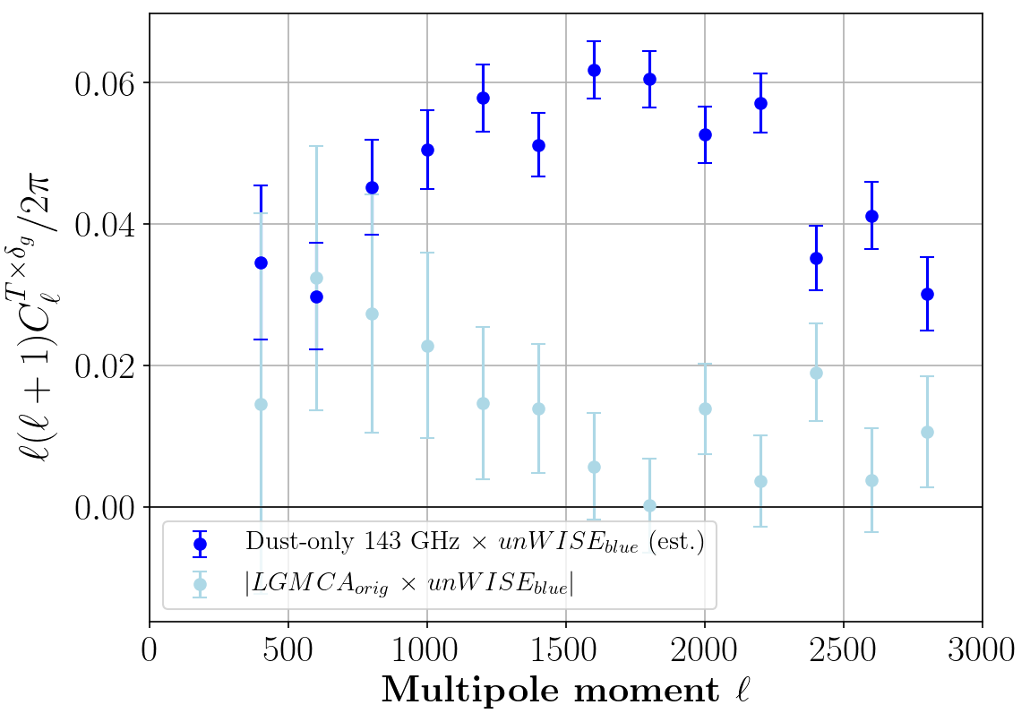
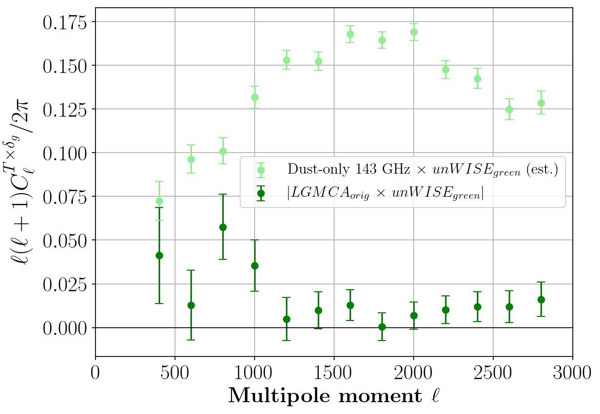
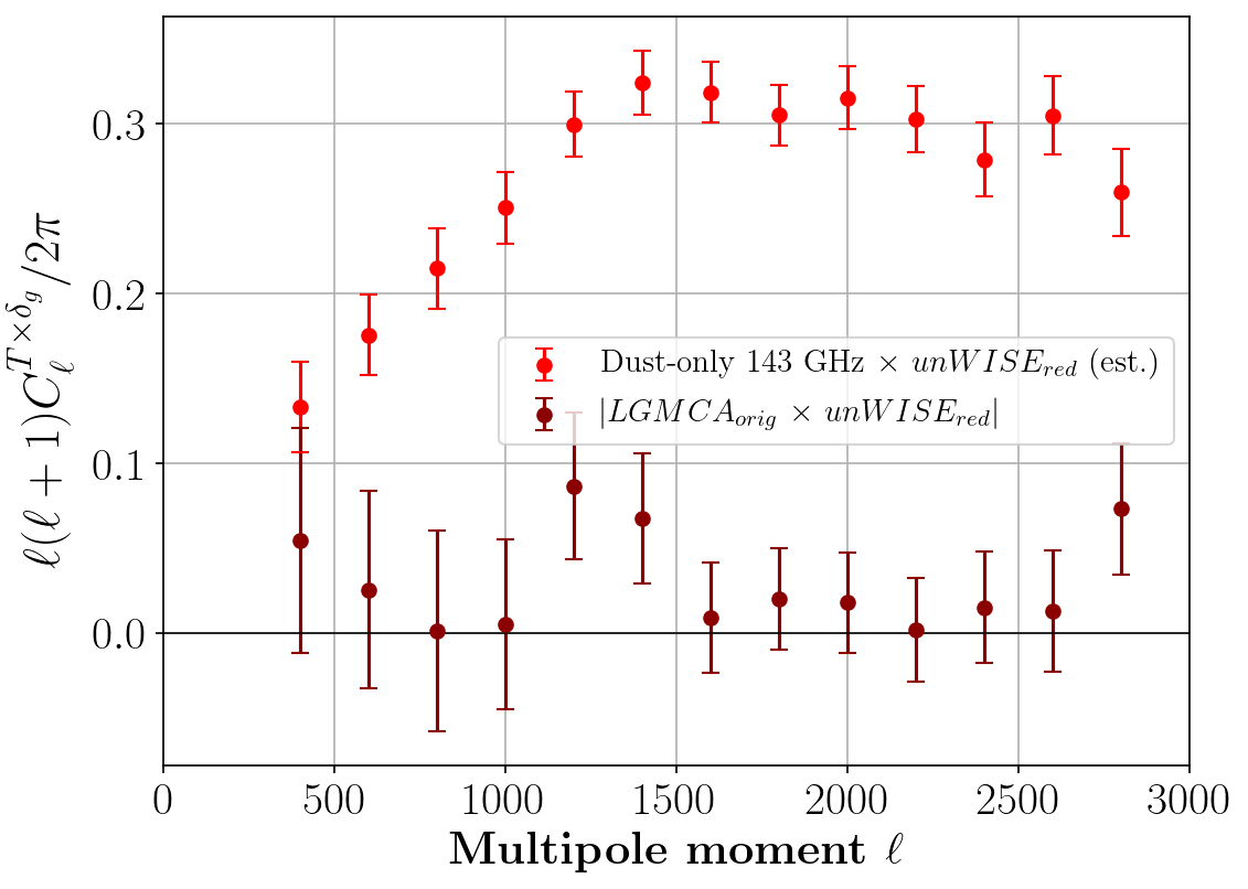
Figure 8: To assess the “additional cleaning factor” described in Appendix B, we show a comparison of the absolute value of $D_{\ell}$ for LGMCA $\times$ unWISE and $D_{\ell}$ for an estimate of the dust-only contribution to 143 GHz $\times$ unWISE, where the latter has been obtained by rescaling from Planck 217 GHz $\times$ unWISE using a dust SED determined from 217 and 545 GHz data (see the text for details). We show these quantities for each of the unWISE maps (color-coded).

$\ell$	blue	green	red
400	2	2	2
600	1	8	7
800	2	2	203
1000	2	4	50
1200	4	32	3
1400	4	16	5
1600	11	13	35
1800	312	301	15
2000	4	24	18
2200	16	15	167
2400	2	12	19
2600	11	10	24
2800	3	8	4

Table 7: The “additional cleaning factors” used to assess how much the original LGMCA cleaning method has reduced the dust compared to its value at 143 GHz. The “additional cleaning factor” for each of the unWISE samples is estimated from the ratio of $\lvert{\rm LGMCA}\times unWISE\rvert$ to our estimate of the dust-only contribution to 143 GHz $\times$ unWISE, which we obtain by measuring Planck 217 GHz $\times$ unWISE and rescaling it with our dust SED model to 143 GHz.

Finally, our (Planck 545 GHz$)^{2}$ $\times$ unWISE measurement rescaled to 143 GHz frequency (so divided by $328.5^{2}$), and then further divided by the additional $\ell$-dependent cleaning factor (also squared), are shown in Fig. 9, and compared with our best-fit kSZ signal. This demonstrates that the dust contamination, even in the original (non-$\alpha$-cleaned) LGMCA map is indeed negligible.

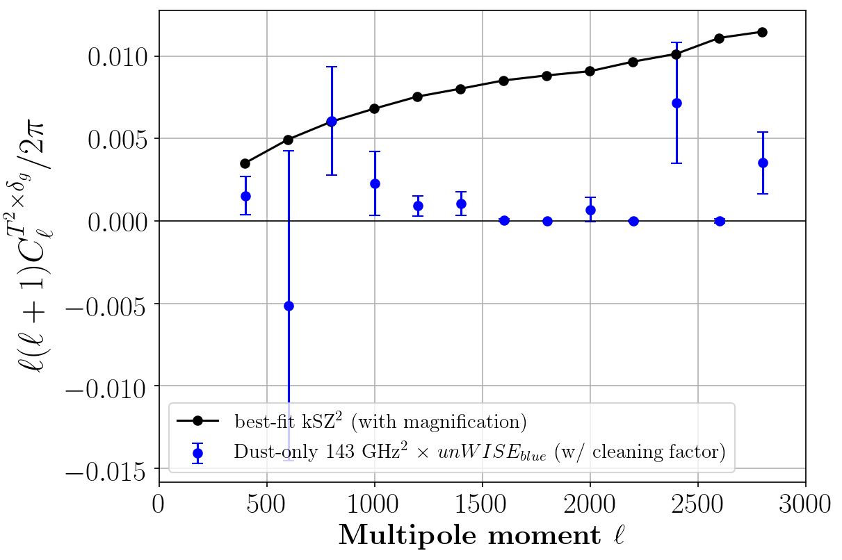
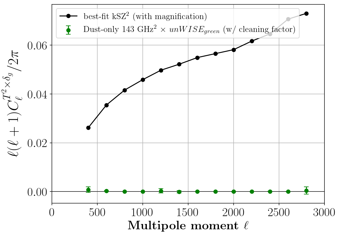
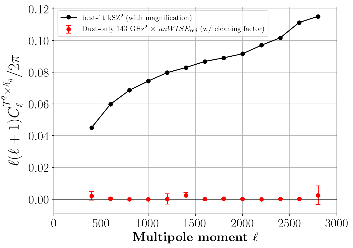
Figure 9: A comparison of the dust contamination present in the LGMCA map versus the best-fit kSZ signal from our analysis for each of the unWISE maps. The dust is assessed by rescaling (Planck 545 GHz)${}^{2}\times unWISE$ down to 143 GHz and dividing by the “additional cleaning factors” from Table 7 squared. This demonstrates that any unWISE-correlated dust that is present in the LGMCA maps is negligible, and we can safely assume it is not a source of our detected signal.

In addition, note that the additional cleaning factor was obtained for the original LGMCA map (before the implementation of any $\alpha$-cleaning method), so the dust contamination will be even more negligible for the LGMCA_clean (i.e., $T_{\rm clean}$, see Eq. 20) map used in our kSZ analysis. Therefore we can safely state that residual unWISE-correlated thermal dust emission present in the LGMCA map yields a negligible bias to the measured kSZ signal in this work.

Appendix C Posteriors of the model parameters

In this appendix, we present the full posterior distributions for the fit parameters: the amplitude of the kSZ² signal, $A_{{\rm kSZ}^{2}}$; the galaxy bias, $b_{g}$; and the magnification response, $s$, for each of the unWISE samples (solid, color-coded lines in Fig. 10). They are obtained by fitting the model in Eq. 21 to the data points in Fig. 5 with a Gaussian likelihood function using the Python emcee package. External priors on $b_{g}$ and $s$ are imposed in this analysis, as described in Section V. In particular, we impose a Gaussian prior on $b_{g}$ for each sample with standard deviation equal to the error bars found in Ref. Krolewski et al. (2020), and a Gaussian prior on $s$ with fractional width of $10\%$.

We also perform the fit without imposing external priors on the galaxy bias $b_{g}$, as a cross-check of our main results. The posterior distributions from this MCMC run are shown in Fig. 10 in dashed lines. They are consistent with our main analysis, which confirms that our data and model yield $b_{g}$ values consistent with those found in Ref. Krolewski et al. (2020). This verifies that our use of the priors based on that work is statistically sound, i.e., we are not imposing an inconsistent assumption on our data.

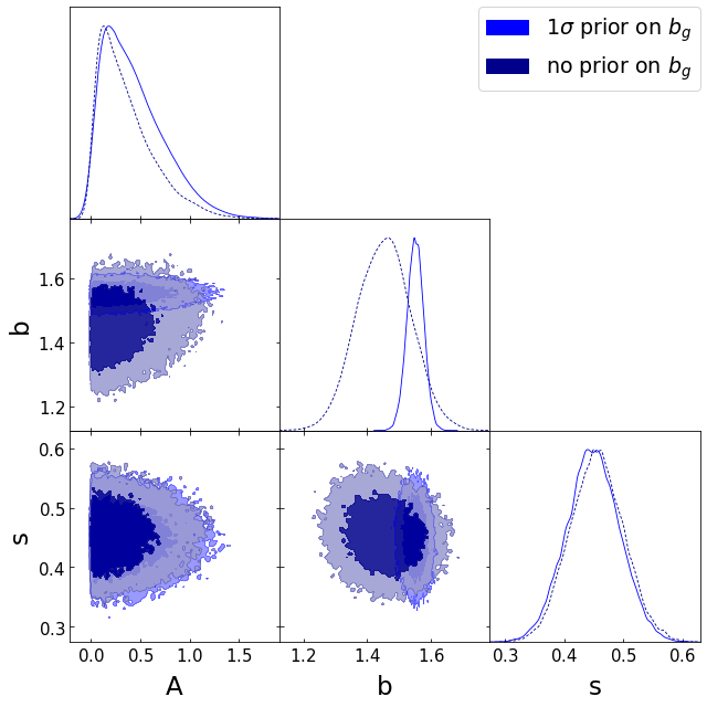
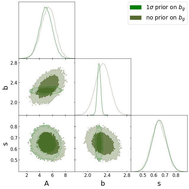
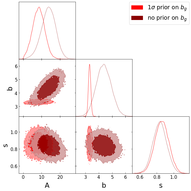
Figure 10: The 2D and 1D marginalized posterior distributions of the $A_{{\rm kSZ}^{2}}$, $b_{g}$, and $s$ parameters for the fit to the cross-power spectra of the product of filtered LGMCA_clean and SMICA with each of the unWISE galaxy maps (solid lines). This analysis imposes external priors on $b_{g}$ and $s$ derived from Ref. Krolewski et al. (2020). The $b_{g}$ priors are Gaussians with mean and 1$\sigma$ width corresponding to the values in Table 4, while the $s$ priors are Gaussians centered at the values in Table 4 with a fractional standard deviation of 10%. The dashed curves are the posteriors of the same model fit, but without the external priors on $b_{g}$. Clockwise from top-left: unWISE blue, green, and red.

Appendix D The 1-halo term for kSZ with projected fields

To build confidence and further understanding of our estimator for $C_{\ell}^{{\rm kSZ}^{2}\times\delta_{g}}$, we present the first computation of the 1-halo term within the halo model formalism. For details about the halo model and its assumptions we refer the reader to the review by Cooray & Sheth Cooray and Sheth (2002). Our goal here is to illustrate the sensitivity of $C_{\ell}^{{\rm kSZ}^{2}\times\delta_{g}}$ to the Halo Occupation Distribution (HOD), i.e., to the distribution of galaxies within halos, and to the properties of the electron gas (velocity and profile). We leave the presentation of a detailed analysis, including the 2-halo and 3-halo terms, for a future paper.

The projected field power spectrum $C_{\ell}^{{\rm kSZ}^{2}\times\delta_{g}}$ is an integral of a bispectrum over a range of scales, modulated by a Wiener filter and beam function to account for the resolution of the CMB maps (see Section II.1). The bispectrum contains two copies of the electron momentum field and one copy of the galaxy overdensity field. An expression for the 1-halo term of the bispectrum is given in Eq. B60 of Coulton et al. (2018). The main feature of this formulation is that the product of the electron momentum fields is written as the product the electron density fields times the cluster velocity dispersion. The cluster velocity dispersion can then be approximated with the RMS of the matter velocity field,

$$v_{\mathrm{rms}}^{2}\left(z\right)=\frac{1}{2\pi^{2}}\int\mathrm{d}k\left[f\left(z\right)a\left(z\right)H\left(z\right)\right]^{2}P\left(k,z\right),$$ (22)

and factored out of the mass integral (see, e.g. Section V D of Hill, 2018). In this equation, $P(k,z)$ is the matter power spectrum and $f$ is the logarithmic derivative of the growth function. In our fiducial model we use the matter power spectrum including non-linear corrections computed with Halofit Takahashi et al. (2012). Meanwhile, the electron density field multiplied by the Thomson cross-section can be interpreted as an optical depth profile and referred to as a $\tau$-profile.

More explicitly, the 1-halo term is computed as

$$C_{\ell}^{{\rm kSZ}^{2}\times\delta_{g},\mathrm{1h}}=\int\frac{d^{2}\ell^{\prime}}{\left(2\pi\right)^{2}}f\left(|\vec{\ell}-\vec{\ell}^{\prime}|\right)f\left(\ell^{\prime}\right)B_{|\vec{\ell}-\vec{\ell}^{\prime}|\ell^{\prime}\ell}^{{\rm kSZ}^{2}\times\delta_{g},\mathrm{1h}},$$ (23)

where the function $f$ is the product of a filter and beam, as in Eq. 4. The 1-halo term of the bispectrum at multipoles $(\ell_{1},\ell_{2},\ell_{3})$ is given by

$$B^{{\rm kSZ}^{2}\times\delta_{g},\mathrm{1h}}_{\ell_{1},\ell_{2},\ell_{3}}=\int\mathrm{d}\eta\,\eta^{2}\frac{v_{\mathrm{rms}}^{2}}{3c^{2}}\int\mathrm{d}M\frac{\mathrm{d}N}{\mathrm{d}M\mathrm{d}V}u_{\ell_{1}}^{\tau}u_{\ell_{2}}^{\tau}u_{\ell_{3}}^{g},$$ (24)

where $\eta$ is the comoving distance, $v_{\mathrm{rms}}^{2}$ is the velocity dispersion given in Eq. (22), $\frac{\mathrm{d}N}{\mathrm{d}M\mathrm{d}V}$ is the differential number of halos per unit mass and volume determined by the halo mass function, $u_{\ell}^{\tau}$ is the 2D Fourier transform of the halo optical depth profile, and $u_{\ell}^{g}$ is the 2D Fourier transform of the halo density profile populated with galaxies. The optical depth term depends on halo masses and redshift and can be written as

$$u_{\ell}^{\tau}(M,z)=W_{\tau}(z)C_{\tau}(M,z)\phi_{\ell}(M,z),$$ (25)

where the redshift dependent term is given by

$$W_{\tau}(z)=\frac{1}{D_{A}(z)^{2}}\frac{\sigma_{\mathrm{T}}}{m_{\mathrm{p}}\mu_{\mathrm{e}}}f_{\mathrm{b}}f_{\mathrm{free}},$$ (26)

where $D_{A}(z)$ is the angular diameter distance, $m_{\mathrm{p}}$ is the proton mass, $\mu_{\mathrm{e}}$ is the mean molecular weight per free electron. It is computed in terms of the primordial hydrogen mass fraction $X_{\mathrm{H}}$ as $\mu_{\mathrm{e}}=2/(1+X_{\mathrm{H}})\simeq 1.14$ for the fiducial value $X_{\mathrm{H}}=0.76$. Assuming that the electron density within halos follows that of matter approximated by the Navarro-Frenk-White (NFW) profile Navarro et al. (1997), the term $C_{\tau}(M,z)$, which depends on mass and redshift but not on multipole, sets the normalization of the $\tau$-profile in terms of the concentration $c_{{}_{\mathrm{NFW}}}$, i.e.,

$$C_{\tau}(M,z)=M\left[\ln(1+c_{{}_{\mathrm{NFW}}})-\frac{c_{{}_{\mathrm{NFW}}}}{1+c_{{}_{\mathrm{NFW}}}}\right]^{-1}.$$ (27)

The last term in Eq. (25) is the 2D Fourier transform of the 3D density profile projected along the LOS, written in a dimensionless fashion and with its normalisation factored out in $C_{\tau}$. With the NFW profile, it reads as

$$\phi_{\ell}(M,z)=\int\mathrm{d}x\frac{x}{(1+x)^{2}}\mathrm{sinc}\left(\frac{\ell+\tfrac{1}{2}}{\ell_{s}}x\right)$$ (28)

with the radial variable $x=r/r_{\mathrm{s}}$, where the characteristic multipole is $\ell_{\mathrm{s}}=D_{A}/r_{\mathrm{s}}$ and the scale radius $r_{\mathrm{s}}=r_{{}_{\mathrm{NFW}}}/c_{{}_{\mathrm{NFW}}}$. Since the integral in Eq. (28) is divergent, it is carried out from the center $x=0$ (or $r=0$) to a limiting $x_{\mathrm{out}}=\Delta c_{{}_{\mathrm{NFW}}}$ (or equivalently $r=\Delta r_{{}_{\mathrm{NFW}}}$, where $\Delta$ is a numerical factor). To choose the outer cut-off radius we compare the prediction of the lensing power spectrum computed within the halo-model and within Halofit, as in Hill and Spergel (2014). We perform the comparison numerically using the public code class_sz Bolliet et al. (2018). In our settings, with fiducial cosmological parameters, halo mass function from Tinker et al. (2010) and concentration from Duffy et al. (2008) both defined with respect to the overdensity masses $M_{200m}$ (hence, $r_{{}_{\mathrm{NFW}}}=r_{200m}$ and $c_{{}_{\mathrm{NFW}}}=c_{200m}$) we find that $\Delta=1$ ensures a nearly perfect match between both methods, over all multipoles of interest. Setting an upper bound to the the radial integration is equivalent to taking the Fourier transform of the NFW profile truncated at $r_{{}_{\mathrm{trunc}}}=\Delta r_{{}_{\mathrm{NFW}}}$. Fortunately, this Fourier transform has an analytical expression (see, e.g., Eq. 18 of Koukoufilippas et al., 2020) which can be used to speed up the numerical computation of the bispectrum without loss of accuracy. Nevertheless, note that assuming a rescaled NFW profile for the electron density is a strong assumption. Indeed, it already appears to be invalidated by recent kSZ measurements Schaan et al. (2020, 2020). But it provides a useful starting point and further work will investigate the validity of this hypothesis, for instance by considering electron density profiles directly calibrated on simulations Battaglia (2016), or by measuring them from data Battaglia et al. (2019).

The galaxy term entering the bispectrum can be written as

$$u_{\ell}^{g}(M,z)=W_{g}(z)\left[U_{\ell}^{g}(M,z)^{2}+2U_{\ell}^{g}(M,z)\right]^{1/2},$$ (29)

with

$$U_{\ell}^{g}(M,z)=N_{\mathrm{sat}}(M,z)\phi_{\ell}^{g}(M,z),$$ (30)

where $N_{\mathrm{sat}}(M,z)$ is determined by a specific HOD and $\phi_{\ell}^{g}(M,z)$ is the Fourier transform of a truncated NFW profile. The profile is truncated at the same radius as before, namely $r_{{}_{\mathrm{trunc}}}=\Delta r_{{}_{\mathrm{NFW}}}$ with $r_{{}_{\mathrm{NFW}}}=r_{200m}$ and $\Delta=1$ in our case. The redshift dependent term is given by

$$W_{g}(z)=\frac{H}{c\eta^{2}}\frac{\varphi_{g}^{\prime}(z)}{\bar{n}_{g}(z)}$$ (31)

where $\varphi_{g}^{\prime}(z)$ is the normalized differential galaxy distribution of the studied sample, i.e.,

$$\varphi_{g}^{\prime}(z)=\frac{1}{N_{g}^{\mathrm{tot}}}\frac{\mathrm{d}N_{g}}{\mathrm{d}z},\quad\mathrm{with}\quad N_{g}^{\mathrm{tot}}=\int\mathrm{d}z\frac{\mathrm{d}N_{g}}{\mathrm{d}z},$$ (32)

the total number of galaxies in the sample and $\bar{n}_{g}(z)$ is the galaxy number density predicted within the HOD model in terms of central and satellite galaxy populations, namely

$$\bar{n}_{g}(z)=\int\mathrm{d}M\frac{\mathrm{d}N}{\mathrm{d}M\mathrm{d}V}\left\{N_{\mathrm{cent}}(M,z)+N_{\mathrm{sat}}(M,z)\right\}.$$ (33)

For central and satellite galaxy populations we use slightly modified version of Eq. (B1) and Eq. (B2) from Krolewski et al. (2020). In particular, we find that replacing $\log_{10}M_{\mathrm{cut}}$ by $1.03\log_{10}M_{\mathrm{cut}}$, and using 1.3 instead of 0.1 in the numerator of Eq. (B2) provides a good fit to the galaxy-galaxy and CMB lensing-galaxy auto and cross power spectra measurements from Krolewski et al. (2020). (Note that these numbers are relevant to the green sample of $unWISE$ galaxies and may differ slightly for the red and blue sample.)

In Fig. 11, we compare the halo model prediction for this HOD (red curves) to the data (black data points). We show results only for the unWISE green sample, as this was the sample that yielded results most discrepant with our fiducial theoretical model in the main analysis, and thus we want to validate the theory calculation. Here our comparison is tentative as our goal is to set the HOD parameter values approximately rather than precisely, since this is enough to check the consistency between our fiducial template for $C_{\ell}^{{\rm kSZ}^{2}\times\delta_{g}}$ and the halo model predictions. But in principle, one could perform a maximum likelihood analysis to set the HOD parameters based on such measurements, eventually enabling constraints on the parameters of the cluster optical depth profile with measurements of $C_{\ell}^{{\rm kSZ}^{2}\times\delta_{g}}$. This point can be directly appreciated by looking at Fig. 12. There, once the HOD parameters have been fixed thanks to the comparison shown in Fig. 11, we plotted the 1-halo term of the kSZ²-galaxy (top panel) and kSZ²-lensing magnification (bottom panel) cross power spectra under three different assumptions for the kSZ effect. These are compared with the template for $C_{\ell}^{{\rm kSZ}^{2}\times\delta_{g}}$ and $C_{\ell}^{{\rm kSZ}^{2}\times\mu_{g}}$ (solid black lines) used in the data analysis presented in the main part of this paper (see, e.g., Fig. 6). Our fiducial halo model (dash-dotted red curves) is consistent with the templates at small scales: at $\ell\approx 3000$, they agree within $5-10\%$. Furthermore, the 1-halo term seems to be the main contribution to $C_{\ell}^{{\rm kSZ}^{2}\times\delta_{g}}$ and $C_{\ell}^{{\rm kSZ}^{2}\times\mu_{g}}$ for $\ell\gtrsim 10^{3}$. By comparing the fiducial halo model (dash-dotted red lines) with the lines labeled as ‘Linear velocity’, we see that non-linear correction to the velocity dispersion (i.e., using the Halofit power spectrum rather than the linear matter power in Eq. 22) is responsible for $20-30\%$ of the power over all scales. Finally, we find that when setting the concentration to the $\tau$-profile twice as high as for the fiducial halo model, the amplitudes of both power spectra increase significantly. Note that as we change $c_{{}_{\mathrm{NFW}}}$ in the $\tau$-profile, we impose that $M_{{}_{\mathrm{NFW}}}$, the total mass enclosed within $r_{{}_{\mathrm{NFW}}}$, remains the same so that on large angular scales $u_{\ell}^{\tau}\propto M_{{}_{\mathrm{NFW}}}$ also remains the same. In this case the main effect of changing the concentration is via its effect on the characteristic multipole $\ell_{\mathrm{s}}$ that enters Eq. (28). It is important to emphasize that we do not expect the large scale power of $C_{\ell}^{{\rm kSZ}^{2}\times\delta_{g}}$ to remain the same here, even though we impose constant $M_{\mathrm{NFW}}$. Indeed, this observable is an integral over a bispectrum and the small scales of the bispectrum (so-called squeezed triangles) also contribute to the large scale amplitude of $C_{\ell}^{{\rm kSZ}^{2}\times\delta_{g}}$ (see Eq. 23) and $C_{\ell}^{{\rm kSZ}^{2}\times\mu_{g}}$.

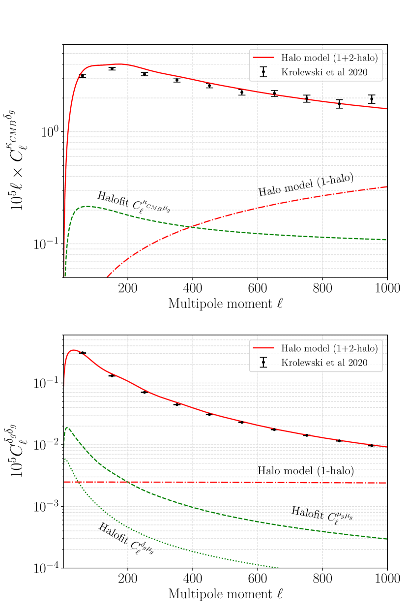
Figure 11: Dimensionless CMB lensing-galaxy cross power spectrum (top panel) and galaxy auto power spectrum (bottom panel). Measurements from Krolewski et al. (2020) are shown as the black data points with error bars. The halo model prediction (1+2-halo) is shown as the solid red lines. The 1-halo term contribution is shown as the dash-dotted red lines. The other curves (in green) show the contribution from lensing magnification bias and are computed according to Eq. 6.4 and 6.5 of Krolewski et al. (2020), using the matter power spectrum computed with Halofit. For this figure we use the green sample of unWISE galaxies and carry out all the Halofit and halo model computations with class_sz.

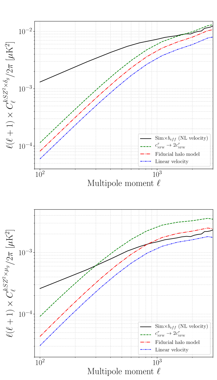
Figure 12: Halo model predictions for the one-halo term contribution to $C_{\ell}^{{\rm kSZ}^{2}\times\delta_{g}}$ (top panel) and $C_{\ell}^{{\rm kSZ}^{2}\times\mu_{g}}$ (bottom panel) under three different assumptions: (i) fiducial halo model (dash-dotted red lines); (ii) velocity dispersion computed without non-linear corrections in the matter power spectrum, i.e., using the linear matter power spectrum rather than Halofit in Eq. 22 (dot-dot-dashed blue lines); (iii) a $\tau$-profile concentration twice as high as the fiducial model (green dashed lines). Note that as we change the concentration we keep the total mass fixed (see text). The solid black lines depict the templates used in the data analysis in the main part of this paper (see Fig. 6). For this figure we use the green sample of unWISE galaxies and carry out all the halo model computations with class_sz. In future work we will compute the other halo-model contributions to these signals, beyond the one-halo term.

Appendix E Validation plots

We present dust tests results for the $\alpha$-cleaned SMICA-noSZ map (see Sec. IV.1 for an analogous cleaning with LGMCA), which are consistent with null (Fig. 13). We also show validation plots to our main analysis, described in details in Sec. VI: (SMICA-noSZ$\cdot$SMICA) $\times$ unWISE in Fig. 14, LGMCA${}^{2}\times$ unWISE in Fig. 15, and SMICA-noSZ${}^{2}\times$ unWISE in Fig. 16, along with their comparison in Figs. 17 and 18.

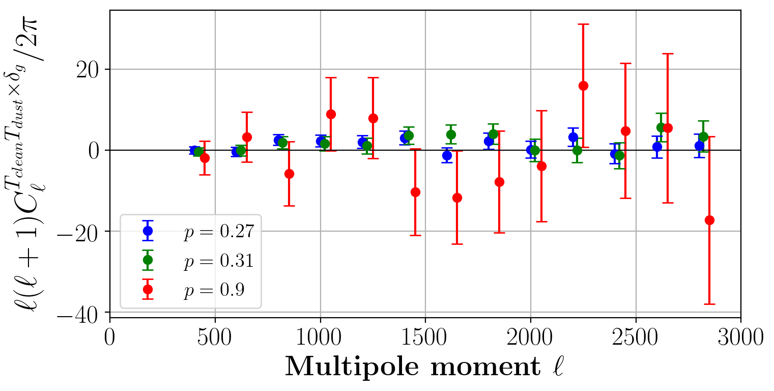
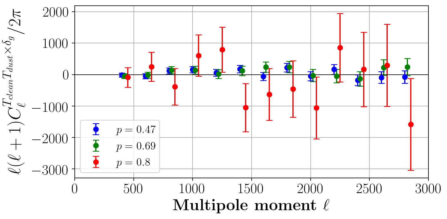
Figure 13: Dust null tests on the $\alpha$-cleaned SMICA-noSZ map, analogous to those shown in Fig. 4 for the $\alpha$-cleaned LGMCA map. We show the dust null tests for the $\alpha$-cleaned LGMCA and $\alpha$-cleaned SMICA-noSZ maps, and not for the original SMICA maps, since the latter has non-negligible tSZ residuals and thus only the former two maps can be used as primary maps in our estimator. All are color coded based on the unWISE subsample colors: blue, red, and green, and the legends give the probabilities-to-exceed for fits to null. The green sample points are offset by $\ell=20$, and the red by $\ell=50$ with respect to the true multipole moment values, for visual purposes. Left: Cross-correlation of $(T_{\rm clean}T_{\rm dust})$ and unWISE, where $T_{\rm dust}$ is the Planck 545 GHz map and $(T_{\rm clean}$ is the clean SMICA-noSZ map. Right: Cross-correlation of $(T_{\rm clean}T_{\rm dust})$ and unWISE, where $T_{\rm dust}$ is the Planck 857 GHz map and $(T_{\rm clean}$ is the clean SMICA-noSZ map. Both are consistent with null.

Figure 14: Cross-power spectra of the real-space product of the cleaned, filtered SMICA-noSZ map and the filtered SMICA map with each of the unWISE galaxy maps: blue, green, and red (data points in respective colors), analogous to our main analysis in Fig. 5. The thin dashed curves show the best-fit lensing contribution, the black dotted are kSZ and the pink stars the residuals. The yellow solid curves in each plot show the total best-fit curves. The best-fit values for the free parameters (the kSZ² amplitude $A_{{\rm kSZ}^{2}}$, galaxy bias $b_{g}$, and the magnification response $s$) are presented in the plot titles. These results validate our main analysis.

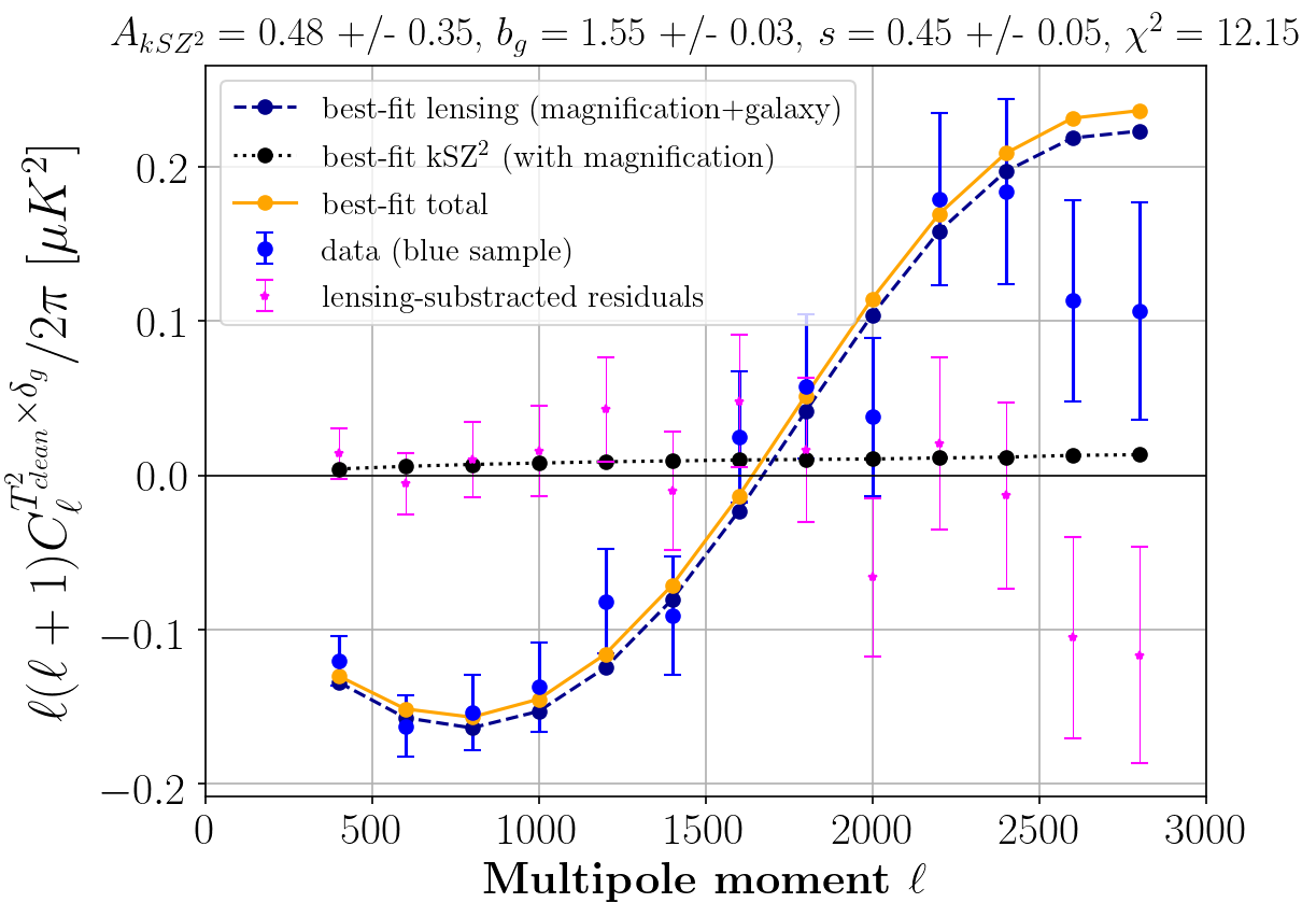
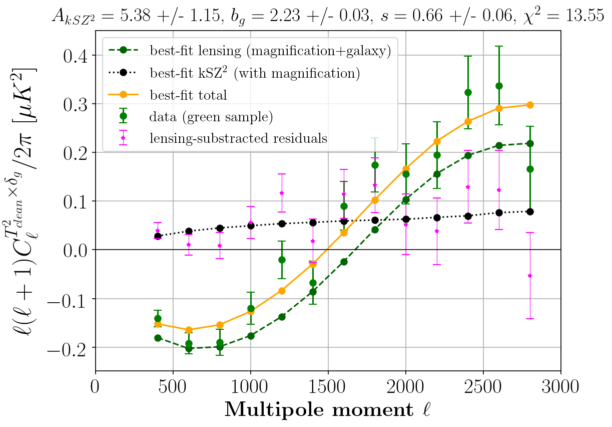
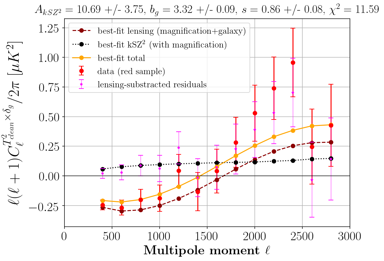
Figure 15: Cross-power spectra of the real-space square of the cleaned, filtered LGMCA map with each of the unWISE galaxy maps: blue, green, and red (data points in respective colors), analogous to our main analysis in Fig. 5. The thin dashed curves show the best-fit lensing contribution, the black dotted the kSZ and the pink stars the residuals. The yellow solid curves in each plot show the total best-fit curves. The best-fit values for the free parameters (the kSZ² amplitude $A_{{\rm kSZ}^{2}}$, galaxy bias $b_{g}$, and the magnification response $s$) are presented in the plot titles. These results validate our main analysis, and also demonstrate that the “asymmetric” estimator employed in our fiducial analysis is robust to foregrounds, while generally yielding smaller error bars than the approach used in these plots (which matches that in H16).

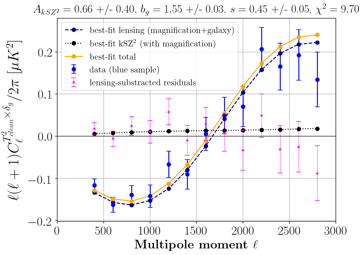
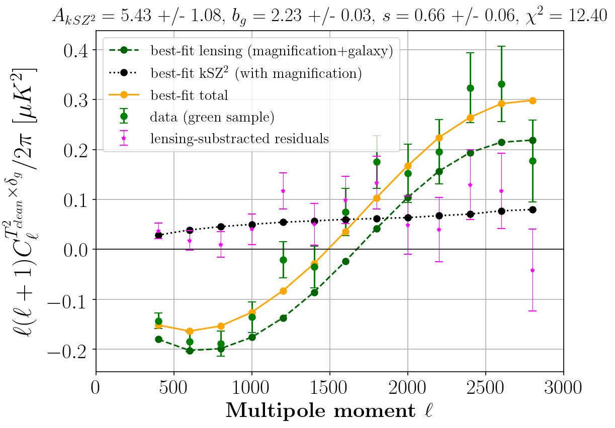
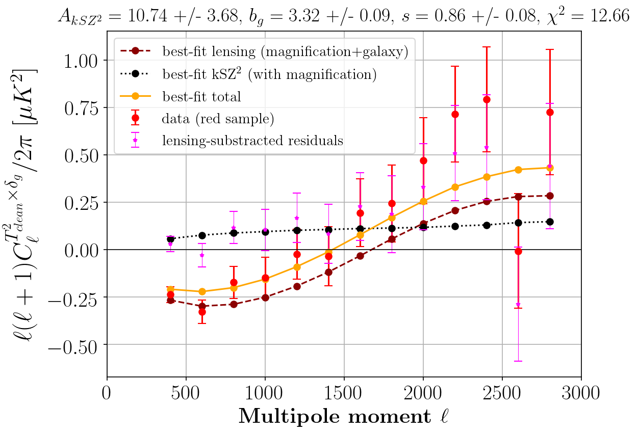
Figure 16: Cross-power spectra of the real-space square of the cleaned, filtered SMICA-noSZ map with each of the unWISE galaxy maps: blue, green, and red (data points in respective colors), analogous to our main analysis in Fig. 5. The thin dashed curves show the best-fit lensing contribution, the black dotted the kSZ and the pink stars the residuals. The yellow solid curves in each plot show the total best-fit curves. The best-fit values for the free parameters (the kSZ² amplitude $A_{{\rm kSZ}^{2}}$, galaxy bias $b_{g}$, and the magnification response $s$) are presented in the plot titles. These results validate our main analysis, and again also verify the robustness of the asymmetric estimator used in our fiducial analysis.

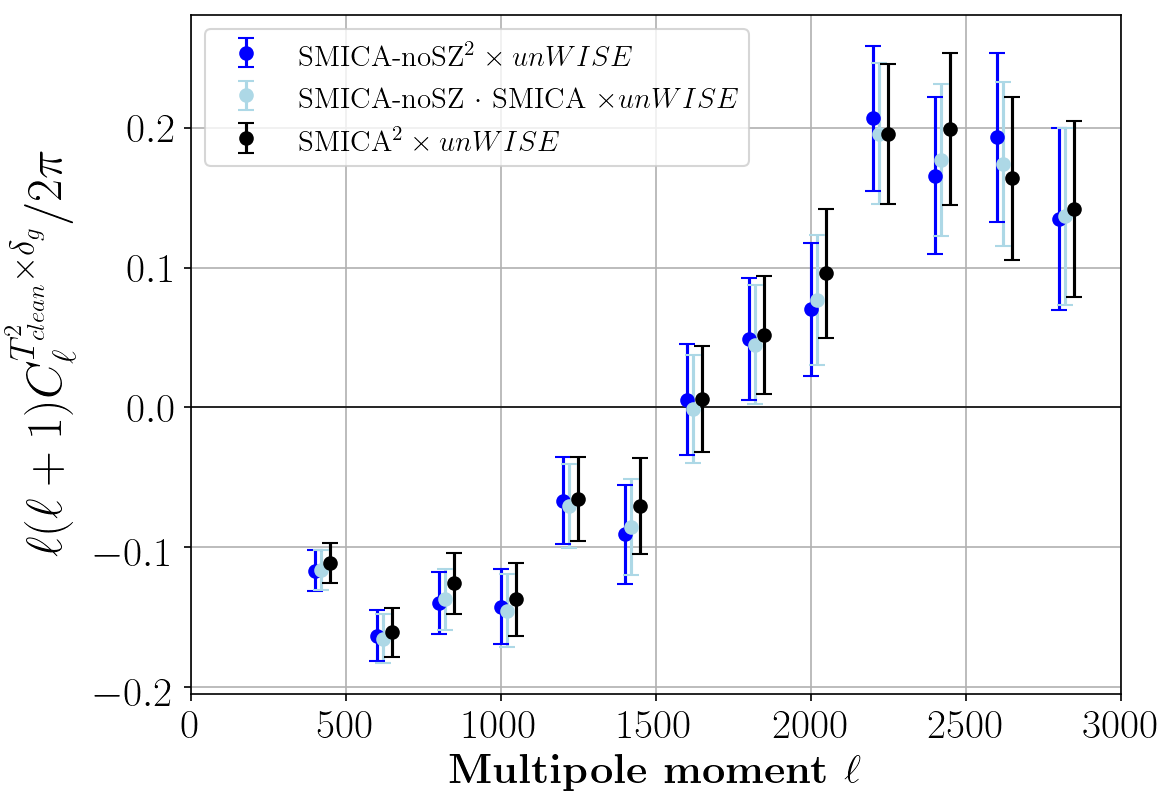
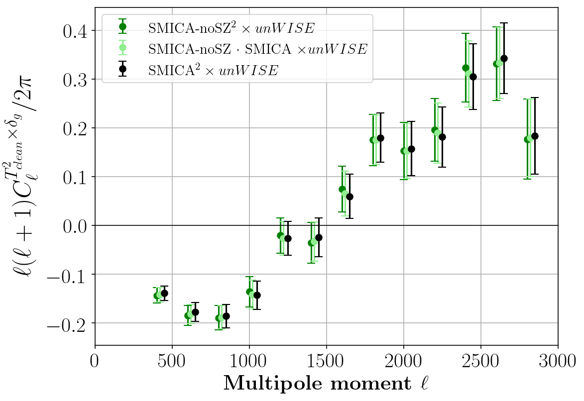
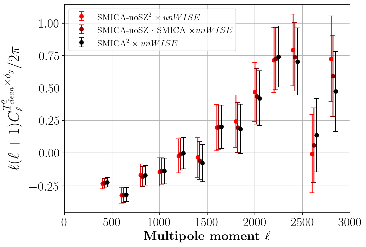
Figure 17: A comparison of all the combinations of SMICA and SMICA-noSZ maps cross-correlated with the unWISE maps (blue, green, and red, color-coded). The (SMICA-noSZ${}_{\rm clean}\cdot$SMICA) $\times$ unWISE points are offset by $\ell=20$, and the SMICA${}_{\rm clean}^{2}$ $\times$ unWISE points are offset by $\ell=50$ with respect to the true multipole moment values, for visual purposes. All analyses yield consistent results with one another, and with our main analysis in Fig. 5, which validates the robustness of our analysis.

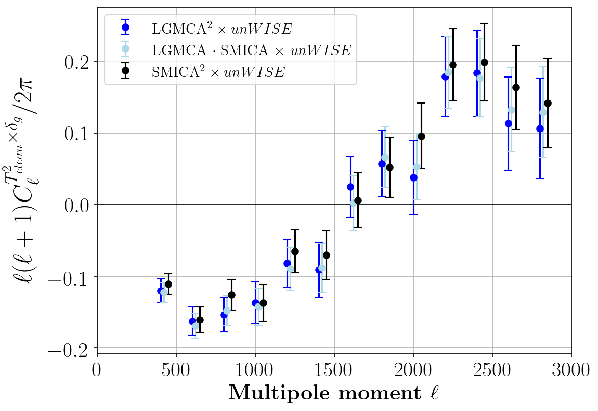
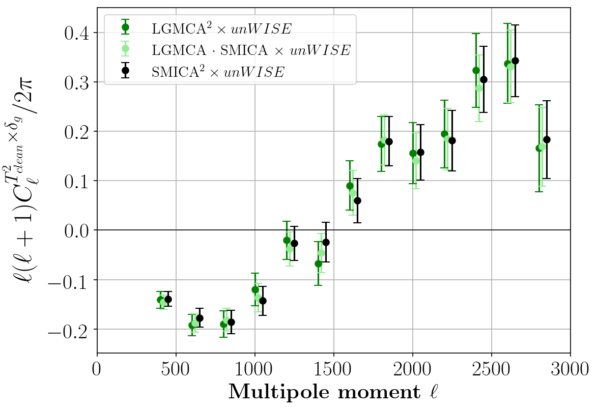
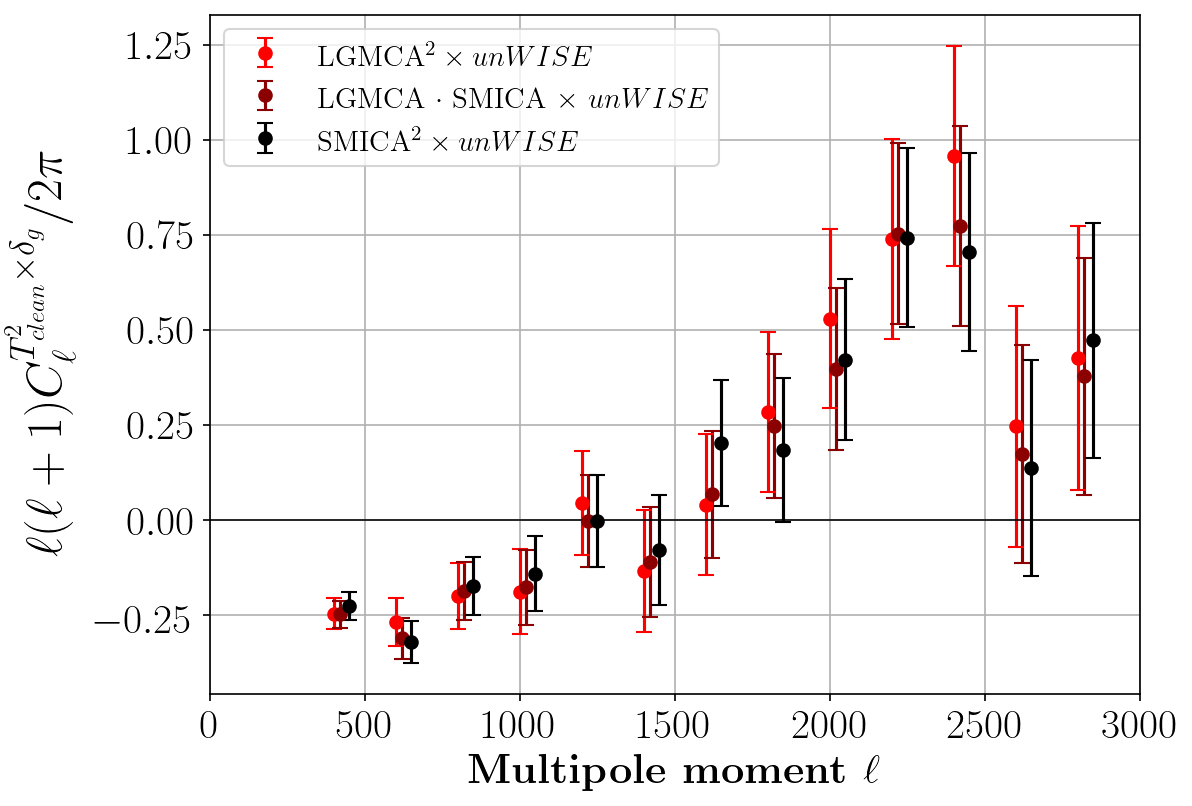
Figure 18: A comparison of all the combinations of SMICA and LGMCA maps cross-correlated with the unWISE maps (blue, green, and red, color-coded). The (LGMCA${}_{\rm clean}\cdot$SMICA) $\times$ unWISE points are offset by $\ell=20$, and the SMICA${}_{\rm clean}^{2}$ $\times$ unWISE points are offset by $\ell=50$ with respect to the true multipole moment values, for visual purposes. All analyses yield consistent results with one another, although the SMICA${}_{\rm clean}^{2}$ results show some small differences, which are likely due to the tSZ residuals present in this map (hence why we do not use this map for our main analysis). Note that our main results from Fig. 5 are also shown here as the cyan, light green, and maroon points, and their consistency with the LGMCA${}_{\rm clean}^{2}$ points validates the robustness of our analysis.

References

- Sunyaev and Zeldovich (1972) R. A. Sunyaev and Y. B. Zeldovich, Comments on Astrophysics and Space Physics 4, 173 (1972).
- Sunyaev and Zeldovich (1980) R. A. Sunyaev and I. B. Zeldovich, Annu. Rev. Astron. Astrophys. 18, 537 (1980).
- Battaglia et al. (2019) N. Battaglia, J. C. Hill, S. Amodeo, J. G. Bartlett, K. Basu, J. Erler, S. Ferraro, L. Hernquist, M. Madhavacheril, M. McQuinn, et al., Probing feedback in galaxy formation with millimeter-wave observations (2019), eprint 1903.04647.
- Bregman (2007) J. N. Bregman, Annu. Rev. Astron. Astrophys. 45, 221 (2007), eprint 0706.1787.
- Ho et al. (2009) S. Ho, S. Dedeo, and D. Spergel, arXiv e-prints arXiv:0903.2845 (2009), eprint 0903.2845.
- Battaglia et al. (2017) N. Battaglia, S. Ferraro, E. Schaan, and D. N. Spergel, J. Cosm. Astrop. Phys. 2017, 040 (2017), eprint 1705.05881.
- Zeldovich and Sunyaev (1969) Y. B. Zeldovich and R. A. Sunyaev, Astroph. and Space Science 4, 301 (1969).
- Hand et al. (2012) N. Hand, G. E. Addison, E. Aubourg, N. Battaglia, E. S. Battistelli, D. Bizyaev, J. R. Bond, H. Brewington, J. Brinkmann, B. R. Brown, et al., Physical Review Letters 109 (2012), ISSN 1079-7114, URL http://dx.doi.org/10.1103/PhysRevLett.109.041101.
- Hill et al. (2016) J. C. Hill, S. Ferraro, N. Battaglia, J. Liu, and D. N. Spergel, Phys. Rev. Lett. 117, 051301 (2016), eprint 1603.01608.
- Ade et al. (2016) P. A. R. Ade, N. Aghanim, M. Arnaud, M. Ashdown, E. Aubourg, J. Aumont, C. Baccigalupi, A. J. Banday, R. B. Barreiro, and et al., Astronomy & Astrophysics 586, A140 (2016), ISSN 1432-0746, URL http://dx.doi.org/10.1051/0004-6361/201526328.
- Macquart et al. (2020) J. P. Macquart, J. X. Prochaska, M. McQuinn, K. W. Bannister, S. Bhandari, C. K. Day, A. T. Deller, R. D. Ekers, C. W. James, L. Marnoch, et al., Nature (London) 581, 391 (2020), eprint 2005.13161.
- Schaan et al. (2020) E. Schaan, S. Ferraro, S. Amodeo, N. Battaglia, S. Aiola, J. E. Austermann, J. A. Beall, R. Bean, D. T. Becker, R. J. Bond, et al., The Atacama Cosmology Telescope: Combined kinematic and thermal Sunyaev-Zel’dovich measurements from BOSS CMASS and LOWZ halos (2020), eprint 2009.05557.
- Schaan et al. (2020) E. Schaan, S. Ferraro, S. Amodeo, N. Battaglia, S. Aiola, J. E. Austermann, J. A. Beall, R. Bean, D. T. Becker, R. J. Bond, et al., arXiv e-prints arXiv:2009.05557 (2020), eprint 2009.05557.
- Sayers et al. (2013) J. Sayers, T. Mroczkowski, M. Zemcov, P. M. Korngut, J. Bock, E. Bulbul, N. G. Czakon, E. Egami, S. R. Golwala, P. M. Koch, et al., The Astrophysical Journal 778, 52 (2013), ISSN 1538-4357, URL http://dx.doi.org/10.1088/0004-637X/778/1/52.
- Ferraro et al. (2016) S. Ferraro, J. C. Hill, N. Battaglia, J. Liu, and D. N. Spergel, Phys. Rev. D 94, 123526 (2016), eprint 1605.02722.
- Soergel et al. (2016) B. Soergel, S. Flender, K. T. Story, L. Bleem, T. Giannantonio, G. Efstathiou, E. Rykoff, B. A. Benson, T. Crawford, S. Dodelson, et al., Monthly Notices of the Royal Astronomical Society 461, 3172–3193 (2016), ISSN 1365-2966, URL http://dx.doi.org/10.1093/mnras/stw1455.
- Schaan et al. (2016) E. Schaan, S. Ferraro, M. Vargas-Magaña, K. M. Smith, S. Ho, S. Aiola, N. Battaglia, J. R. Bond, F. De Bernardis, E. Calabrese, et al., Physical Review D 93 (2016), ISSN 2470-0029, URL http://dx.doi.org/10.1103/PhysRevD.93.082002.
- Sayers et al. (2019) J. Sayers, A. Montaña, T. Mroczkowski, G. W. Wilson, M. Zemcov, A. Zitrin, N. Cibirka, S. Golwala, D. Hughes, D. Nagai, et al., The Astrophysical Journal 880, 45 (2019), ISSN 1538-4357, URL http://dx.doi.org/10.3847/1538-4357/ab29ef.
- Tanimura et al. (2020) H. Tanimura, S. Zaroubi, and N. Aghanim, Direct detection of the kinetic Sunyaev-Zel’dovich effect in galaxy clusters (2020), eprint 2007.02952.
- Doré et al. (2004) O. Doré, J. F. Hennawi, and D. N. Spergel, Astrophys. J. 606, 46 (2004), eprint astro-ph/0309337.
- DeDeo et al. (2005) S. DeDeo, D. N. Spergel, and H. Trac, arXiv e-prints astro-ph/0511060 (2005), eprint astro-ph/0511060.
- Planck Collaboration et al. (2016) Planck Collaboration, P. A. R. Ade, N. Aghanim, M. Arnaud, M. Ashdown, J. Aumont, C. Baccigalupi, A. J. Banday, R. B. Barreiro, J. G. Bartlett, et al., Astron. Astrophys. 594, A13 (2016), eprint 1502.01589.
- Steigman (2007) G. Steigman, Annual Review of Nuclear and Particle Science 57, 463–491 (2007), ISSN 1545-4134, URL http://dx.doi.org/10.1146/annurev.nucl.56.080805.140437.
- Wright et al. (2010) E. L. Wright, P. R. M. Eisenhardt, A. K. Mainzer, M. E. Ressler, R. M. Cutri, T. Jarrett, J. D. Kirkpatrick, D. Padgett, R. S. McMillan, M. Skrutskie, et al., Astron. J. 140, 1868 (2010), eprint 1008.0031.
- Mainzer et al. (2011) A. Mainzer, J. Bauer, T. Grav, J. Masiero, R. M. Cutri, J. Dailey, P. Eisenhardt, R. S. McMillan, E. Wright, R. Walker, et al., Astrophys. J. 731, 53 (2011), eprint 1102.1996.
- Cutri et al. (2013) R. M. Cutri, E. L. Wright, T. Conrow, J. W. Fowler, P. R. M. Eisenhardt, C. Grillmair, J. D. Kirkpatrick, F. Masci, H. L. McCallon, and S. L. Wheelock, Tech. Rep. (2013).
- Mainzer et al. (2014) A. Mainzer, J. Bauer, R. M. Cutri, T. Grav, J. Masiero, R. Beck, P. Clarkson, T. Conrow, J. Dailey, P. Eisenhardt, et al., Astrophys. J. 792, 30 (2014), eprint 1406.6025.
- Meisner et al. (2017a) A. M. Meisner, D. Lang, and D. J. Schlegel, Astron. J. 153, 38 (2017a), eprint 1603.05664.
- Meisner et al. (2017b) A. M. Meisner, D. Lang, and D. J. Schlegel, Astron. J. 154, 161 (2017b), eprint 1705.06746.
- Meisner et al. (2018) A. M. Meisner, D. Lang, and D. J. Schlegel, Research Notes of the American Astronomical Society 2, 1 (2018), eprint 1801.03566.
- Meisner et al. (2019) A. M. Meisner, D. Lang, E. F. Schlafly, and D. J. Schlegel, Proc. of the Astron. Soc. of the Pacific 131, 124504 (2019), eprint 1909.05444.
- Schlafly et al. (2019) E. F. Schlafly, A. M. Meisner, and G. M. Green, The Astrophysical Journal Supplement Series 240, 30 (2019), eprint 1901.03337.
- Schlafly et al. (2018) E. F. Schlafly, G. M. Green, D. Lang, T. Daylan, D. P. Finkbeiner, A. Lee, A. M. Meisner, D. Schlegel, and F. Valdes, The Astrophysical Journal Supplement Series 234, 39 (2018), eprint 1710.01309.
- Krolewski et al. (2020) A. Krolewski, S. Ferraro, E. F. Schlafly, and M. White, J. Cosm. Astrop. Phys. 2020, 047 (2020), eprint 1909.07412.
- Gaia Collaboration et al. (2016) Gaia Collaboration, T. Prusti, J. H. J. de Bruijne, A. G. A. Brown, A. Vallenari, C. Babusiaux, C. A. L. Bailer-Jones, U. Bastian, M. Biermann, D. W. Evans, et al., Astron. Astrophys. 595, A1 (2016), eprint 1609.04153.
- Gaia Collaboration et al. (2018) Gaia Collaboration, A. G. A. Brown, A. Vallenari, T. Prusti, J. H. J. de Bruijne, C. Babusiaux, C. A. L. Bailer-Jones, M. Biermann, D. W. Evans, L. Eyer, et al., Astron. Astrophys. 616, A1 (2018), eprint 1804.09365.
- Bobin et al. (2013) J. Bobin, J.-L. Starck, F. Sureau, and S. Basak, Astronomy & Astrophysics 550, A73 (2013), ISSN 1432-0746, URL http://dx.doi.org/10.1051/0004-6361/201219781.
- Bobin et al. (2014) J. Bobin, F. Sureau, J.-L. Starck, A. Rassat, and P. Paykari, Astronomy & Astrophysics 563, A105 (2014), ISSN 1432-0746, URL http://dx.doi.org/10.1051/0004-6361/201322372.
- Madhavacheril and Hill (2018) M. S. Madhavacheril and J. C. Hill, Phys. Rev. D 98, 023534 (2018), eprint 1802.08230.
- Adam et al. (2016) R. Adam, P. A. R. Ade, N. Aghanim, M. Arnaud, M. Ashdown, J. Aumont, C. Baccigalupi, A. J. Banday, R. B. Barreiro, and et al., Astronomy & Astrophysics 594, A9 (2016), ISSN 1432-0746, URL http://dx.doi.org/10.1051/0004-6361/201525936.
- Planck Collaboration et al. (2018a) Planck Collaboration, N. Aghanim, Y. Akrami, M. Ashdown, J. Aumont, C. Baccigalupi, M. Ballardini, A. J. Banday, R. B. Barreiro, N. Bartolo, et al., arXiv e-prints arXiv:1807.06209 (2018a), eprint 1807.06209.
- Battaglia et al. (2010) N. Battaglia, J. R. Bond, C. Pfrommer, J. L. Sievers, and D. Sijacki, The Astrophysical Journal 725, 91–99 (2010), ISSN 1538-4357, URL http://dx.doi.org/10.1088/0004-637X/725/1/91.
- Battaglia et al. (2013) N. Battaglia, A. Natarajan, H. Trac, R. Cen, and A. Loeb, The Astrophysical Journal 776, 83 (2013), ISSN 1538-4357, URL http://dx.doi.org/10.1088/0004-637X/776/2/83.
- Limber (1957) D. N. Limber, Astrophys. J. 125, 9 (1957).
- LoVerde and Afshordi (2008) M. LoVerde and N. Afshordi, Phys. Rev. D 78, 123506 (2008), eprint 0809.5112.
- Gil-Marín et al. (2012) H. Gil-Marín, C. Wagner, F. Fragkoudi, R. Jimenez, and L. Verde, Journal of Cosmology and Astroparticle Physics 2012, 047–047 (2012), ISSN 1475-7516, URL http://dx.doi.org/10.1088/1475-7516/2012/02/047.
- Lewis and Challinor (2006) A. Lewis and A. Challinor, Phys. Rep. 429, 1 (2006), eprint astro-ph/0601594.
- Ferraro and Hill (2018) S. Ferraro and J. C. Hill, Phys. Rev. D 97, 023512 (2018), eprint 1705.06751.
- Blas et al. (2011) D. Blas, J. Lesgourgues, and T. Tram, Journal of Cosmology and Astroparticle Physics 2011, 034–034 (2011), ISSN 1475-7516, URL http://dx.doi.org/10.1088/1475-7516/2011/07/034.
- Takahashi et al. (2012) R. Takahashi, M. Sato, T. Nishimichi, A. Taruya, and M. Oguri, The Astrophysical Journal 761, 152 (2012), ISSN 1538-4357, URL http://dx.doi.org/10.1088/0004-637X/761/2/152.
- Bennett et al. (2013) C. L. Bennett, D. Larson, J. L. Weiland, N. Jarosik, G. Hinshaw, N. Odegard, K. M. Smith, R. S. Hill, B. Gold, M. Halpern, et al., Astrophys. J. Supp. 208, 20 (2013), eprint 1212.5225.
- Bobin et al. (2014) J. Bobin, F. Sureau, J. L. Starck, A. Rassat, and P. Paykari, Astron. Astrophys. 563, A105 (2014), eprint 1401.6016.
- Planck Collaboration et al. (2018b) Planck Collaboration, Y. Akrami, M. Ashdown, J. Aumont, C. Baccigalupi, M. Ballardini, A. J. Band ay, R. B. Barreiro, N. Bartolo, S. Basak, et al., arXiv e-prints arXiv:1807.06208 (2018b), eprint 1807.06208.
- Sultan Abylkairov et al. (2020) Y. Sultan Abylkairov, O. Darwish, J. C. Hill, and B. D. Sherwin, arXiv e-prints arXiv:2012.04032 (2020), eprint 2012.04032.
- Darwish et al. (2021) O. Darwish, M. S. Madhavacheril, B. D. Sherwin, S. Aiola, N. Battaglia, J. A. Beall, D. T. Becker, J. R. Bond, E. Calabrese, S. K. Choi, et al., Mon. Not. R. Astron. Soc. 500, 2250 (2021), eprint 2004.01139.
- Abbott et al. (2021) T. M. C. Abbott, M. Adamow, M. Aguena, S. Allam, A. Amon, S. Avila, D. Bacon, M. Banerji, K. Bechtol, M. R. Becker, et al., arXiv e-prints arXiv:2101.05765 (2021), eprint 2101.05765.
- Wright et al. (2010) E. L. Wright, P. R. M. Eisenhardt, A. K. Mainzer, M. E. Ressler, R. M. Cutri, T. Jarrett, J. D. Kirkpatrick, D. Padgett, R. S. McMillan, M. Skrutskie, et al., The Astronomical Journal 140, 1868–1881 (2010), ISSN 1538-3881, URL http://dx.doi.org/10.1088/0004-6256/140/6/1868.
- Newman (2008) J. A. Newman, The Astrophysical Journal 684, 88–101 (2008), ISSN 1538-4357, URL http://dx.doi.org/10.1086/589982.
- McQuinn and White (2013) M. McQuinn and M. White, Monthly Notices of the Royal Astronomical Society 433, 2857–2883 (2013), ISSN 1365-2966, URL http://dx.doi.org/10.1093/mnras/stt914.
- Laigle et al. (2016) C. Laigle, H. J. McCracken, O. Ilbert, B. C. Hsieh, I. Davidzon, P. Capak, G. Hasinger, J. D. Silverman, C. Pichon, J. Coupon, et al., The Astrophysical Journal Supplement Series 224, 24 (2016), ISSN 1538-4365, URL http://dx.doi.org/10.3847/0067-0049/224/2/24.
- Eisenhardt et al. (2020) P. R. M. Eisenhardt, F. Marocco, J. W. Fowler, A. M. Meisner, J. D. Kirkpatrick, N. Garcia, T. H. Jarrett, R. Koontz, E. J. Marchese, S. A. Stanford, et al., Astrophys. J. Supp. 247, 69 (2020), eprint 1908.08902.
- Planck Collaboration et al. (2014) Planck Collaboration, P. A. R. Ade, N. Aghanim, C. Armitage-Caplan, M. Arnaud, M. Ashdown, F. Atrio-Barandela, J. Aumont, C. Baccigalupi, A. J. Banday, et al., Astron. Astrophys. 571, A9 (2014), eprint 1303.5070.
- Alonso et al. (2019) D. Alonso, J. Sanchez, and A. Slosar, Monthly Notices of the Royal Astronomical Society 484, 4127–4151 (2019), ISSN 1365-2966, URL http://dx.doi.org/10.1093/mnras/stz093.
- Senn (2019 (accessed December, 2020) M. Senn, NaMaster (2019 (accessed December, 2020)), URL https://github.com/LSSTDESC/NaMaster.
- Foreman-Mackey et al. (2013) D. Foreman-Mackey, D. W. Hogg, D. Lang, and J. Goodman, Proc. of the Astron. Soc. of the Pacific 125, 306 (2013), eprint 1202.3665.
- Nelson et al. (2019) D. Nelson, A. Pillepich, V. Springel, R. Pakmor, R. Weinberger, S. Genel, P. Torrey, M. Vogelsberger, F. Marinacci, and L. Hernquist, Monthly Notices of the Royal Astronomical Society 490, 3234–3261 (2019), ISSN 1365-2966, URL http://dx.doi.org/10.1093/mnras/stz2306.
- Pillepich et al. (2019) A. Pillepich, D. Nelson, V. Springel, R. Pakmor, P. Torrey, R. Weinberger, M. Vogelsberger, F. Marinacci, S. Genel, A. van der Wel, et al., Monthly Notices of the Royal Astronomical Society 490, 3196–3233 (2019), ISSN 1365-2966, URL http://dx.doi.org/10.1093/mnras/stz2338.
- Aiola et al. (2020) S. Aiola, E. Calabrese, L. Maurin, S. Naess, B. L. Schmitt, M. H. Abitbol, G. E. Addison, P. A. R. Ade, D. Alonso, M. Amiri, et al., J. Cosm. Astrop. Phys. 2020, 047 (2020), eprint 2007.07288.
- Naess et al. (2020) S. Naess, S. Aiola, J. E. Austermann, N. Battaglia, J. A. Beall, D. T. Becker, R. J. Bond, E. Calabrese, S. K. Choi, N. F. Cothard, et al., J. Cosm. Astrop. Phys. 2020, 046 (2020), eprint 2007.07290.
- Benson et al. (2014) B. A. Benson, P. A. R. Ade, Z. Ahmed, S. W. Allen, K. Arnold, J. E. Austermann, A. N. Bender, L. E. Bleem, J. E. Carlstrom, C. L. Chang, et al., in Millimeter, Submillimeter, and Far-Infrared Detectors and Instrumentation for Astronomy VII, edited by W. S. Holland and J. Zmuidzinas (2014), vol. 9153 of Society of Photo-Optical Instrumentation Engineers (SPIE) Conference Series, p. 91531P, eprint 1407.2973.
- Ade et al. (2019) P. Ade, J. Aguirre, Z. Ahmed, S. Aiola, A. Ali, D. Alonso, M. A. Alvarez, K. Arnold, P. Ashton, J. Austermann, et al., J. Cosm. Astrop. Phys. 2019, 056 (2019), eprint 1808.07445.
- Abazajian et al. (2019) K. Abazajian, G. Addison, P. Adshead, Z. Ahmed, S. W. Allen, D. Alonso, M. Alvarez, A. Anderson, K. S. Arnold, C. Baccigalupi, et al., arXiv e-prints arXiv:1907.04473 (2019), eprint 1907.04473.
- Madhavacheril et al. (2020) M. S. Madhavacheril, J. C. Hill, S. Næss, G. E. Addison, S. Aiola, T. Baildon, N. Battaglia, R. Bean, J. R. Bond, E. Calabrese, et al., Phys. Rev. D 102, 023534 (2020), eprint 1911.05717.
- Ma et al. (2018) Q. Ma, K. Helgason, E. Komatsu, B. Ciardi, and A. Ferrara, Mon. Not. R. Astron. Soc. 476, 4025 (2018), eprint 1712.05305.
- La Plante et al. (2020) P. La Plante, A. Lidz, J. Aguirre, and S. Kohn, Astrophys. J. 899, 40 (2020), eprint 2005.07206.
- Górski et al. (2005) K. M. Górski, E. Hivon, A. J. Banday, B. D. Wandelt, F. K. Hansen, M. Reinecke, and M. Bartelmann, Astrophys. J. 622, 759 (2005), eprint arXiv:astro-ph/0409513.
- Zonca et al. (2019) A. Zonca, L. Singer, D. Lenz, M. Reinecke, C. Rosset, E. Hivon, and K. Gorski, Journal of Open Source Software 4, 1298 (2019), URL https://doi.org/10.21105/joss.01298.
- Cooray and Sheth (2002) A. Cooray and R. K. Sheth, Phys. Rept. 372, 1 (2002), eprint astro-ph/0206508.
- Coulton et al. (2018) W. R. Coulton et al., JCAP 09, 022 (2018), eprint 1711.07879.
- Hill (2018) J. C. Hill, Physical Review D 98 (2018), ISSN 2470-0029, URL http://dx.doi.org/10.1103/PhysRevD.98.083542.
- Navarro et al. (1997) J. F. Navarro, C. S. Frenk, and S. D. M. White, The Astrophysical Journal 490, 493–508 (1997), ISSN 1538-4357, URL http://dx.doi.org/10.1086/304888.
- Hill and Spergel (2014) J. C. Hill and D. N. Spergel, Journal of Cosmology and Astroparticle Physics 2014, 030–030 (2014), ISSN 1475-7516, URL http://dx.doi.org/10.1088/1475-7516/2014/02/030.
- Bolliet et al. (2018) B. Bolliet, B. Comis, E. Komatsu, and J. F. Macías-Pérez, Mon. Not. Roy. Astron. Soc. 477, 4957 (2018), eprint 1712.00788.
- Tinker et al. (2010) J. L. Tinker, B. E. Robertson, A. V. Kravtsov, A. Klypin, M. S. Warren, G. Yepes, and S. Gottlöber, The Astrophysical Journal 724, 878–886 (2010), ISSN 1538-4357, URL http://dx.doi.org/10.1088/0004-637X/724/2/878.
- Duffy et al. (2008) A. R. Duffy, J. Schaye, S. T. Kay, and C. Dalla Vecchia, Monthly Notices of the Royal Astronomical Society: Letters 390, L64–L68 (2008), ISSN 1745-3933, URL http://dx.doi.org/10.1111/j.1745-3933.2008.00537.x.
- Koukoufilippas et al. (2020) N. Koukoufilippas, D. Alonso, M. Bilicki, and J. A. Peacock, Mon. Not. Roy. Astron. Soc. 491, 5464 (2020), eprint 1909.09102.
- Battaglia (2016) N. Battaglia, J. Cosm. Astrop. Phys. 2016, 058 (2016), eprint 1607.02442.