How many phases nucleate in the
bidimensional Potts model?
Abstract
We study the kinetics of the two-dimensional -state Potts model after a shallow quench slightly below the critical temperature and above the pseudo spinodal. We use numerical methods and we focus on intermediate values of , . We show that, initially, the system evolves as if it were quenched to the critical temperature. The further decay from the metastable state occurs by nucleation of out of the possible phases. For a given quench temperature, is a logarithmically increasing function of the system size. This unusual finite size dependence is a consequence of a scaling symmetry underlying the nucleation phenomenon for these parameters.
1 Introduction
When a control parameter is changed in such a way that a thermodynamical system undergoes a first-order phase transition one observes hysteresis and metastability. These phenomena are widespread in nature [1] and, particularly, in many areas of physics [2, 3, 4, 1, 5]. Besides, metastability plays a prominent role also in biological systems such as, for instance, proteins and nucleic acids [6, 7].
The simplest example of metastability is, perhaps, a uniaxial ferromagnet in an external field, whose paradigmatic modelisation is the Ising model. Upon field reversal, provided that its magnitude is sufficiently small and the temperature is subcritical, the magnetisation remains at the pre-reversal value for a certain time, the lifetime of the metastable state, before flipping to the new equilibrium value. The phenomenon can be ascribed to the competition between surface tension and bulk energy and is accounted for, at least at a simple semi-quantitative level, by classical nucleation theory [1, 8, 9, 10]: a nucleus of the equilibrium phase in a metastable sea is unstable unless its size exceeds a critical value. If it is not the case it disappears. Then, in this picture, the lifetime of the metastable state is the time needed to nucleate, by thermal fluctuations, a critical nucleus (notice that in this context critical does not refer to the criticality of the state at ). Elaborating on these ideas, more refined theories of nucleation [11, 12, 13, 14, 15, 16, 17, 18, 19, 20, 21, 22] have been developed, and they describe the phenomenon with good accuracy.
In the previous example, the metastable and equilibrium states are associated to the two ergodic components which characterise the system al low temperatures. However, the situation is not as well understood in systems with more ergodic components, such as those described at the simplest level by the ferromagnetic Potts model [23]. This model is defined in terms of lattice discrete variables taking possible values, sometimes called colours, and the interaction favours equal colour on nearest neighbour sites. For , the Ising model is recovered.
In the absence of external fields, the Potts model undergoes a phase transition between a high temperature disordered phase and a low temperature, symmetry broken, ordered one at a -dependent critical temperature . In two dimensions, the character of the transition changes crossing [24, 25]: for it is continuous (second order), while for it is discontinuous (first order) and metastability is found. Specifically, upon quenching from to a finite-size system remains for some time in the disordered state before starting the evolution towards the final equilibrium state. The usual interpretation is that the metastable state is the (single) ergodic component at while the target equilibrium state is one of the symmetry-related ergodic components at . Hence, at variance with the field-driven transition in the Ising model, nucleation occurs towards a -degenerate final state, and one speaks of multi-nucleation. Another important difference is that the transition is temperature driven.
To determine the lifetime of the metastable state, its dependence on the system size, the dynamic escape from it, and the nature of the nucleation process is a difficult and much debated issue [26, 27, 28, 29]. In particular, it was argued [30, 31, 32, 33] that both the lifetime of the metastable state and temperature range below where it takes place shrink when the system size increases. This intriguing feature, which has no analog in the discontinuous field-driven transition of the Ising model, poses yet unresolved questions on the nature of the metastable state in the thermodynamic limit. In a previous paper [34], some of us addressed this problem analytically with a perturbation scheme valid for large . It turns out that, for , a long lived metastable state exists for quenches to final temperatures , where . In [34] a rather precise description of the metastable state was given, both from the microscopic and thermodynamic points of view. However, a similar characterisation of the escape kinetics is still missing for finite . Specifically, while the nature of the metastable state can be well described in such an analytical framework, its lifetime (for finite ) has not been determined yet and its very existence in the thermodynamic limit cannot be proved. Related to this issue, the order in which the two limits of large and large system size should be taken remains to be clarified.
In this paper we study the process whereby the disordered metastable state is run away and how the target equilibrium state is approached in the square lattice Potts model with , after shallow quenches from high to low temperatures close to . We use Monte Carlo numerical simulations with the Metropolis rule for different values of and linear system sizes . We choose values which are larger than , , but not too large so that we can observe nucleation in a relatively wide temperature interval below , see [34]. In a companion paper by some of us [35] the related issue of deep quenches below the pseudo-spinodal of the same model for much larger values, closer to the ideal limit, is tackled and the full parameter dependence of the curvature-driven growing length in the coarsening regime is determined.
Our main result is the characterisation of the multi-nucleation process. We show that, soon after the quench, the system evolves as if it were at the critical temperature. Later, multi-nucleation takes over. We prove that for a given system size, the number of phases that nucleate is a logarithmically increasing function of , see Eq. (15). In addition, we also study the dependence of on and . Phases which do not nucleate disappear from the system immediately after the metastable state is escaped. Those which nucleate start competing, resulting in a coarsening process [36, 37, 38, 39, 40, 35, 41, 42, 43, 44, 45, 46] which leads, at some point, to the progressive elimination of the less represented colours until symmetry is definitively broken, one single colour survives, and equilibrium is attained (at not too low temperatures; otherwise, blocked states of the kind discussed in [36, 37, 38, 39, 40, 35] can stop the evolution).
The paper is organised as follows. In Sec. 2 we introduce the Potts model and its dynamics. We also define the relevant observables that will be further considered. In Sec. 3 we provide a general description of the whole dynamical process, from the instant of the quench, to the escape from metastability and further on. Section 4 is the core of the article and contains a thorough discussion of the multi-nucleation process. Finally, Sec. 5 concludes the paper.
2 Model and observables
The Hamiltonian of the Potts model [23] reads
| (1) |
where is a coupling constant and are nearest-neighbour couples on a two-dimensional lattice of linear dimension which we take to be a square one. is the Kronecker delta and is an integer variable ranging from 1 to . We consider periodic boundary conditions. In the sum we count each bond once, and for this geometry the energy is bounded between and . The critical temperature is exactly known in [23]
| (2) |
and the phase transition is second (first) order for () [47]. Notice that for finite systems of size there are corrections to the value of given for infinite size in Eq. (2) according to [48]. Henceforth we will set .
We consider the dynamics where single spins are updated according to a random sequence with a probability to change from an initial value to a final one . We will use the Metropolis form , where is the energy variation associated to the flip. A unit time, or Montecarlo step, is elapsed after attempted moves.
In the following we will consider a protocol in which the system, initially prepared in an infinite temperature equilibrium state, is suddenly quenched at time to a low temperature . The dynamical evolution has been studied in previous works [35, 36, 37, 43, 41, 42, 44, 45, 46, 38, 39, 40] mainly focusing on the coarsening regime. Here we are more interested in metastability and multi-nucleation, which clearly arise at .
After the quench the system relaxes to a low energy state and the energy density approaches the final equilibrium value . Here and in the following the non equilibrium average is taken over thermal histories and initial conditions. In order to quantify the relaxation, therefore, we will consider the energy density excess
| (3) |
In a state with well formed domains, connected regions with the same spin state, the excess energy is stored on domain walls, and is proportional to the density of interfacial spins. Since for non fractal aggregates this quantity is, in turn, inversely proportional to the typical size of the domains, from one can infer such characteristic length as
| (4) |
We will discuss below another determination of a typical length scale, that should behave in a similar way.
A fundamental quantity, usually considered in coarsening processes, is the equal time spin-spin correlation function. Specifically, we define the quantity
| (5) |
Notice that, due to isotropy and homogeneity, only depends on the distance , where is the vector joining and , and should be independent of and . Hence, further on we will denote it and, enforcing this symmetry, we will rather compute the spatial average of the quantity in Eq. (5), namely . In this way, we will improve the statistics. It is clear that, on the one hand, at (namely ) and, on the other hand, at very large distance, because of the expected factorisation of the first term in the numerator. Defining
| (6) |
Eq. (5) can be re-written as
| (7) |
where
| (8) |
is the correlation function restricted to the colour . Equation (7) transparently expresses the fact that the unrestricted correlation is the weighted average of the restricted ones, the weights being the variances of the Boolean variables associated to , see Eq. (6).
When dynamical scaling holds, takes the form
| (9) |
where is a scaling function and a characteristic size with the meaning of the typical domain’s linear dimension. From the correlation function one can extract such a size in different ways. For instance, one can use the momenta as
| (10) |
In case of dynamical scaling, determinations with different values of provide proportional results (however large values are numerically problematic since the noisy large- tails of are heavily weighted). Similarly, one can use the half-height width to define as
| (11) |
In the following we will use this determination which is easier. Analogously, the typical size of domains of a specific colour can be defined replacing with in Eq. (11):
| (12) |
Let us mention that Eq. (12) cannot be used to determine in two situations: i) The corresponding colour is not present in the system. In this case , Eq. (12) loses its meaning, and could be taken to be identically zero. ii) The colour has invaded the whole system. Also in this case one has , because of the subtraction term in Eq. (8), and one can assume that the size of the domain of colour is the system size . In general, immediately before one of the two situations i), ii) occur, one finds a very small value of . Hence it must be kept in mind that finding a small value of does not necessarily mean that the corresponding colour is present only in small domains, but it could as well be that it has flooded the system. Which case applies must be ascertained differently, for instance, by visual inspection of the configurations. This will be important further on.
Labelling of the possible values of the spins will be done in the following in a dynamical way: at any time we order the colours according to their abundances, from the most to the least represented, and label them with increasing from to . This method is useful, particularly in the late stage of the dynamics where, as we will discuss, a clear hierarchy of abundances sets in. We have checked that some exchanges in the ordering occur during evolution for the values we use here but these are rare. Roughly speaking, a hierarchy of colours is installed when the phases nucleate.
3 The dynamical process
In the following we will discuss the results of the numerical simulations of the Potts model introduced above. We will mainly consider three values, , 24, 100, as paradigms of small, intermediate and large behaviors. Other values have also been studied and we sometimes include them in the presentation. These systems are quenched to final temperatures close to the critical one, , in order to appreciate the metastable state and its lifetime. In most of our simulations we set for , for , and for . These choices are motivated by the requirement to have a comparable nucleation time (see discussion below, and Fig. 1) for the three reference values of . Notice that fixing does not correspond to fixing . Let us also remind that, as discussed below Eq. (2), is the critical temperature of the infinite system. In order to investigate the finite-size effects, a central issue of this paper, we will used systems in the range of sizes (only for qualitative illustrations, such as the snapshots in Fig. 2, we consider systems as small as ). Comparing the value of the equilibrium coherence length at given in [49] with the system sizes we use, one concludes that is at least 13 (in the worst case with ). Therefore our studies are expected to be basically free from the usual equilibrium finite size effects occurring when is smaller or comparable to . This, however, does not exclude other finite size effect of non-equilibrium nature, which are indeed a central point of this article, as we will explain below.
(a) (b)
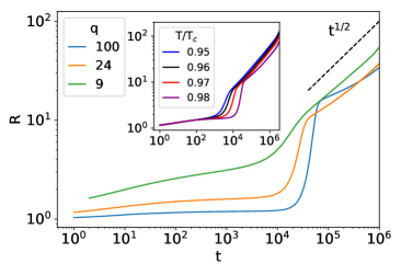
A first qualitative description of the kinetic process after a quench stems from the behavior of , the typical length scale extracted from the analysis of the excess energy as in Eq. (4), which is shown in Fig. 1. With some quantitative differences, the same kind of pattern is observed for any value of (see also [37, 44] and [50] where this quantity, for more and values, respectively, was shown). After a short transient, one can clearly identify three extended regimes. The first one is associated to growing slowly or staying approximately constant, . This plateau, which is flatter and longer as at fixed or as at fixed , is a clear manifestation of metastability. In this time lag the kinetics is useless because the system is confined in a local free energy minimum and the trapping barrier is not yet jumped over. In order to do it, critical nuclei, namely ordered domains of a sufficiently large size, must develop. However, this is an activated process which requires a certain time , the nucleation time. At the system is still in a rather disordered state, visually not too different from the initial one, see the snapshots taken at in Fig. 2. Some small ordered domains can be spotted but they are too tiny to start nucleation.
Actually, this metastable state is similar to the equilibrium one at , in a sense that we are going to specify below. We illustrate this point by means of the correlation function defined in Eq. (5). In Fig. 3 this quantity is plotted against during the evolution after a quench. Let us focus, to start with, on panel (a), where curves for a quench to (continuous lines) are compared to those, taken at the same times, for a quench to (dashed ones). In the latter case one sees that, as time goes on, the correlation extends to larger values of until at the curves start to superimpose, signalling that equilibrium has been reached. At short times, a similar pattern is displayed by the curves of the subcritical quench (continuous ones) which stay close to the ones previously discussed. At longer times, for , the correlations move to the right further than those of the quench to and there is tendency to accumulate on a curve somewhat broader than the equilibrium one at . This occurs roughly in the range of times which corresponds to the lifetime of the metastable state. In this time range the correlation is almost time-independent at short , whereas some evolution can be spotted at large . This signals that the metastable state is not really stable, and that a prodrome of its failure, which can be interpreted as the build up of critical nuclei, is occurring at large distances. Finally, roughly for , a quick growth of correlations is observed, unveiling that metastability is over and that the next stage, where ordering takes place, has been entered. In this case, the classification of the behaviour of the correlation into three stages (initial evolution, stasis, late evolution) is not sharp because, as we discuss below, is relatively far from .
(a) (b) (c)
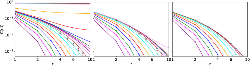
Let us now have a look at the other two panels in Fig. 3. In the central one (b) the quench is closer to and the accumulation of curves in the metastable state is clearer than in the left panel. Furthermore, the locus where superposition occurs is also closer to the equilibrium curve at with respect to what is seen in the left panel. In the right panel (c) the subcritical quench is so close to that the departure from the metastable state cannot even be measured within the simulated times. Besides that, one sees a pattern similar to the one observed in the other panels, with the notable difference that the correlations in the metastable state are almost indistinguishable from the ones of equilibrium at . This clarifies our statement that the metastable state is similar to the equilibrium one at : the closer to the quench is (from below), the longer the life-time of the metastable state and the more similar to equilibrium at it is. More precisely, indicating with a one-time observable measured in a system quenched to , one has , where the latter is the measurement of made in equilibrium at . Clearly, this cannot be true for any function of the state of the system, particularly if it is weighting hugely the large distance features, but the statement is expected to be correct for most quantities of physical interest.
The nucleation time can be roughly identified as the time when the plateau is over and jumps rather abruptly to a higher value, see Fig. 1. This is a violent process corresponding to the fast invasion of available space by the super-critical nuclei, as it can be seen from the snapshots in Fig. 2 corresponding to and . It was shown in [50] that increases exponentially in this time domain. Such speedy relaxation becomes sharper upon increasing .
The duration of the metastable state increases as , as it can be seen in the inset of Fig. 1(a). In the same picture we can also observe that the plateau value is rather -independent while, instead, there is a clear dependence on . In [50] it was found that this value is well approximated by for small () and then, increasing further , it saturates to a value of order one. This dependence can be understood recalling that is the inverse energy density excess (Eq. [4]). The energy density in the metastable state was computed in [34] and goes to zero for large as , where is a temperature dependent factor. On the other hand the asymptotic equilibrium quantity becomes independent on [52] for large . Therefore we conclude that approaches a large- value from below, as observed. Given the choice of temperatures made in Fig. 1(a) (so as to have roughly fixed) it is clear that, working instead at a constant or even at a finite fraction of , i.e. , the lifetime of metastability increases with . Similarly, we have also noticed that the temperature range where metastability occurs widens for larger . Specifically, indicating with the lower temperature where metastability is still observed we find that increases with .
The fast process associated to the steep increase of ends at a time when nuclei of different colour come in contact, a configuration that can be observed in Fig. 2 at times and/or (except for the smallest size where one single colour nucleates, see the discussion in Sec. 4). At this point a coarsening phenomenon sets in produced by the competition among domains, as shown in Fig. 2 and reported in [36, 37, 43, 41, 42, 44, 45, 46, 38] and, for the closely related vector Potts (or clock) model, in [51]. In this kind of evolution one expects dynamical scaling and , which is indeed roughly noted in Fig. 1 at very long times (for this behavior is likely to be reached on times longer than the simulated ones). Since this regime is not the focus of this paper we content with such a semi-quantitative indication.
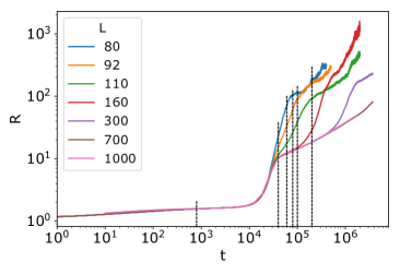
Before closing this section let us comment on the fact that the data for are free from finite-size effects until domains coarsen up to a length comparable to the system size, which occurs at a time . This can be seen in Fig. 1 (b) where one sees that the curves depart from the one corresponding to the larger system size () when . For instance, this occurs at a time of order , and around . However, the fact that this particular quantity () does not feel the size of the system before does not mean that the dynamics is globally free from finite-size effects in this time domain. Actually, in Fig. 2 one clearly sees that the configurations at a given time look very different in systems of different sizes. The next section is devoted to the discussion of this feature.
4 Multi-nucleation
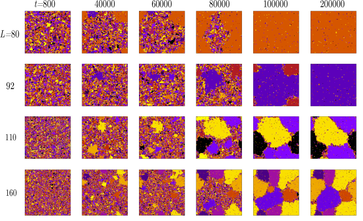
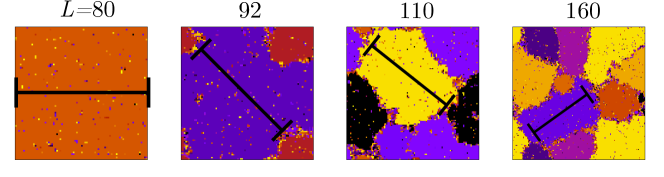
In the introduction we have briefly discussed the fact that, at variance with the Ising field driven first order transition, in the thermal one the role of the system size is important. The reason is that and the pseudo-spinodal temperature depend on system size. In the previous section we have already anticipated that, besides this feature, also the nature of the dynamic escape from the metastable state changes significantly with the system size, as a visual inspection of Fig. 2, where the same quench of the model is operated on systems of different sizes, clearly displays. Specifically, when a relatively small size is considered (, upper row) a single critical droplet forms and grows, invading the whole system (last two snapshots). This is what we call mono-nucleation, or 1-nucleation. We have checked that such phenomenon is observed rather independently of the thermal realisation of the process. Notice that the dominating colour (orange) did not seem to be the favoured one before its outburst (one would have rather predicted the violet or yellow colour as better candidates), a fact that shows the rapidity of critical nucleation.
In the second row the behaviour of a slightly larger system () is shown. This small size increase is sufficient to modify qualitatively the situation, in that there are now two nucleating colours, the red and the violet ones. Then, in this case, we have bi-nucleation, or 2-nucleation. Again, this feature is rather independent of the thermal realisation. After nucleation, surface tension closes the domain of the minority colour (last snapshot), symmetry is definitely broken and equilibrium is attained, but this occurs on much larger times than those of nucleation.
Increasing further the system size as in the two rows below, the fate of a system changes again and one observes 3-nucleation and 6-nucleation. Notice that, after nucleation, the competition among domains of different colours leads to a progressive elimination of their number. Increasing further (not shown) one can observe -nucleation with up to ( in this example).
(a) (b) (c)
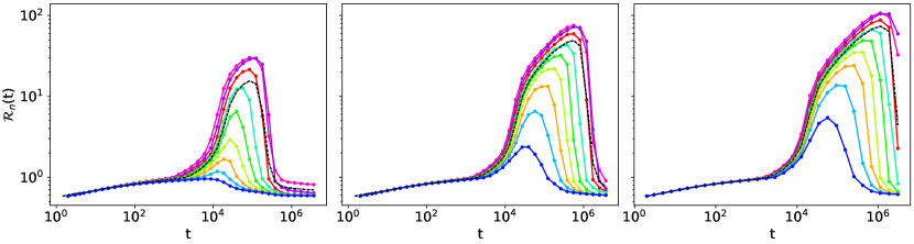
In order to discuss the multi-nucleation process and its dependence on the system size at a more quantitative level we consider the typical lengths of the various colours, , which are shown for three different system sizes in Fig. 4. From this figure one clearly sees that for the various colours initially grow, up to a characteristic time when they reach a maximum and then shrink. This means that domains of the corresponding colour grow, reach a maximum size, and then collapse and disappear. For the prevailing colour (and possibly the next ones in the hierarchy also reaching domain sizes comparable to the system size itself) denoted by #1 in Fig. 4, the interpretation is different, since the final decrease of must be associated to the invasion of the whole space, according to what discussed in case ii) at the end of Sec. 2.
(a) (b)
(c) (d)

From the comparison between the three different system sizes represented in Fig. 4, one can make some remarks. First, it is clear that for small sizes some colours do not nucleate, whereas they do in larger systems. For instance, colour #9, represented in blue, does not show the exponential increase typical of nucleation for and does not go beyond , whereas it does grow significantly in the larger systems with and . This indicates that is a quantity one can use to establish the number of nucleating colours. Secondly, from Fig. 4 one sees that both the peak time and its height are increased in a larger system. Exploiting these two observations we developed a method to determine the number of nucleating phases as a function of and , that we now describe.
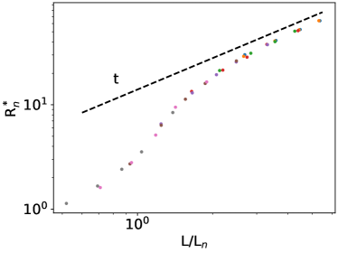
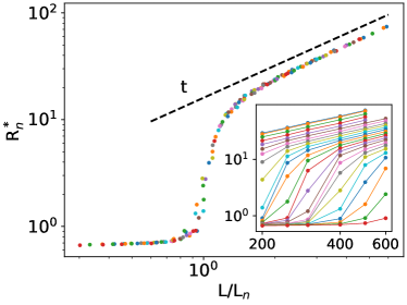
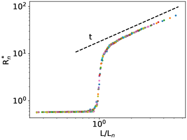
First, we measure for all and different system sizes. This information is summarised for in the inset of Fig. 5 (b). The first three panels of this figure, (a)-(c), which refer to different values of , show that the data very clearly obey a scaling form
| (13) |
where is a fitting parameter which is plotted in Fig. 5 (d). A similar pattern is found for other values of , not reported in the figure. Notice that imposing collapse of the curves according to Eq. (13) only fixes up to an arbitrary multiplicative constant. We fix it by asking that the steep part of be centred at .
The scaling function stays small for , it suddenly increases around (the larger the , the steeper the growth) and it then behaves as for large (see the dashed lines in Fig. 5 (a)-(c)). This latter trend indicates that, for each colour such that the representative point lies in this sector, the maximum size of the domains is triggered linearly by the system size, as it usually happens for a finite size effect in a standard (e.g. binary) coarsening system (see also the discussion at the end of this section). Hence, we argue that points belonging to this sector of , i.e. , correspond to colours that, given the system size , have nucleated. Analogously, points in the small sector, i.e. , where takes an approximately constant small value, correspond to colours that did not succeed nucleating. On the basis of this, we conclude that , namely , is the condition for the -th colour to enter the coarsening stage. In particular, one can interpret as the smallest system size in order to have competition between domains of different colour. This means that such a size must host the largest domain present at when coarsening starts. Hence we conclude that has the physical meaning of the typical size of the largest droplets in the system at the coalition time . This can be appreciated in Fig. 6 where a ruler of length is plotted on top of the configurations of the model at .
We also observe that the small- plateau value of decreases with increasing . This can be explained recalling that points laying there are representative of colours that cannot nucleate, and arguing that, as such, their properties are basically those of the metastable state. The latter, in turn, is akin to the equilibrium state at , as discussed, whose coherence length decreases upon increasing .
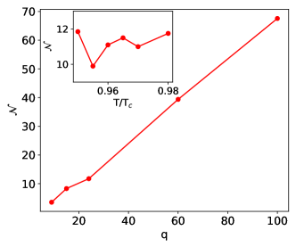
Looking at the plot of in Fig. 5 (d), one finds an exponential dependence
| (14) |
This law describes well all the data for , and the large region for (with fitting parameters , 82.97, 200.00 and , 11.848, 67.568 for , respectively). Furthermore, we found an analogous behaviour for other values of not portrayed in Fig. 5. Repeating the procedure above for different temperatures we find that is, within errors, independent of . This is shown in the inset of Fig. 7 (a) for a fixed value of , in this case. It seems that the behaviour reported can be ascribed more to some random effect, or errors, rather than to a genuine dependence (notice also that the fluctuations of are only around 10% of itself). Similar results are found for other values of . This explains the parameter dependencies written in Eq. (14).
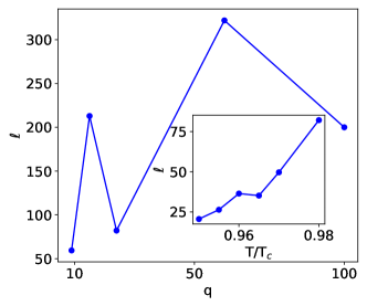
As shown in Fig. 7 (a) turns out to increase in a roughly linear way with . In this case, at variance with the dependence discussed before, the variation of is monotonic and important, as compared to itself. Moving to , its dependence on (at fixed ) can be appreciated in inset of the right panel of Fig. 7, where one finds that increases in a roughly linear way with . On the other hand, with the choice of made in our simulations, which as discussed earlier correspond to fix the lifetime of the metastable state, the dependence of on , shown in the right panel of Fig. 7, cannot be straightforwardly interpreted.
(a) (b)
We now discuss the meaning of the length appearing in Eq. (14). We consider an intermediate range of values of such that the following two conditions are obeyed: a) is sufficiently small as to have the exponential form (14) valid down to (as already commented, this is true for but not for ) and b) . For example, the two conditions are reasonably obeyed for , since . In such an intermediate range of , after Eq. (14) one has , the typical size associated to the prevailing colour whose interpretation was discussed above. Hence amounts to the typical size of the largest droplets in the system at the coalition time . For outside such intermediate range, e.g. for large , we expect to have a related interpretation, even though we cannot derive it directly from Eq. (14). Let us also observe that from Fig. 7 one extrapolates for , implying that the metastable state becomes the stable equilibrium one, as expected.
Coming to the issue of multi-nucleation, applying the argument above to , we can say that the -th colour has nucleated if . Using Eq. (14) we arrive at the conclusion that, given a system size , one has -nucleation with
| (15) |
where the notation simply accounts for the constraint . One can easily check that, using the values of and in this equation, one can correctly predict the number of nucleating colours observed in the various cases of Fig. 2. Notice however that the domain of validity of this equation is inherited by that of Eq. (14), hence if is large it holds true only for sufficiently large values of .
This result shows that, for a given , the number of nucleating phases grows only logarithmically with the system size. When the thermodynamic limit is taken from the onset, all phases nucleate. Also, if the size of the system is large enough, i.e. , increasing reduces the number of nucleating phases. Let us also notice that Eq. (15) informs us on the number of nucleating phases, but does not predict the time needed to nucleate. Clearly, if this time grew towards infinity, no nucleation would be found. In the large -limit, it was also observed that a different mechanism takes over, see for instance Fig. 6(c)(d) in [35], with, possibly, a different scaling of with that still needs to be investigated in depth.
The discussion above shows that the multi-nucleation dynamics of the two dimensional Potts model is interested by peculiar finite size effects, rather different from the usual ones arising in the phase-ordering of binary systems. In the latter, there are only two competing colours and the growth of the domains does not feel the finiteness of the system until some time , when the domains’ size becomes comparable to . At this point the coarsening process is interrupted and the system enters a final stage whereby equilibrium is approached. For times any (intensive) measurement does not depend on the value of . In the Potts model, one observes an analogous behaviour when observing a quantity like , as we discussed at the end of Sec. 3. This is also true also for the sizes and of the two prevailing colours. However, the number of coarsening phases depends on up to a value of as large as , given in Eq. (14). Notice that this characteristic size diverges both as for a given and as for a given , as discussed above. Worst, the sizes () of the domains of the minority colours, do depend on even if measured at times (see Fig. 4). This strange behaviour is perhaps at the origin of many controversies on the size dependence of the metastable dynamics.
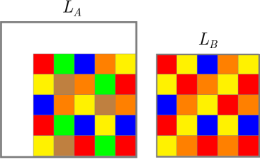
One might wonder how it may be possible that the unrestricted quantity be size-independent whereas the restricted ones do depend on , given that is morally the average of the s. This occurs because only fixes the average size of domains but not their colour, as it is schematically illustrated in Fig. 8. The configuration on the left shows a portion of a system of size at a time where six phases are present. On the right, instead, an analogous system with a different size is represented at the same time . The represented portion of the first system equals the total size of the second. It can be seen that, although two phases (the green and the brown one) are absent in the smaller lattice (hence the number of colours is dependent), the size of the domains does not change (hence is independent).
5 Discussion
In this paper we studied the multi-nucleation phenomenon after a shallow quench of the Potts model with to . A related study of the model with addressing deep quenches to is presented in a companion article by some of us [35].
The main result of this paper, which is contained in Eq. (15), is that the number of nucleating phases of the two-dimensional Potts model with not too large increases logarithmically with the system size. The logarithmic behaviour informs us that this feature cannot be related to the trivial geometrical fact that a larger system can accommodate a larger number of developing colours. If this were the origin, the snapshots in Fig. 2 should display an equal number of nucleating phases in portions with equal area of systems with different sizes. This, however, is not observed. For instance, comparing the systems of relative double size (first line) and (last row), at time , one sees that there is only one nucleating colour (orange, besides a remnant of the disordered phase) in the smallest system, whereas there are typically more than one colour in a portion of area of the system with . This raises an important question which, by the way, concerns also the size dependence of the metastable state recalled in the introduction: how can a system with a very short coherence length (of the order of the nuclei size, as it can also be appreciated from the correlation function of Fig. 3) feel the boundary effects? Rephrased differently, if nucleation is a local process, since correlations are short, how could it be influenced by a global property such as the total size?
Here we provide a possible, although at the moment completely speculative, answer. In a series of papers [53, 54, 55] some of us showed that in a rather broad class of binary models the fate of the system, namely which of the two colours will eventually invade the sample, is decided at a very early stage when a percolation cluster grows as large as the whole sample. Since percolation is an uncorrelated phenomenon, this occurs when spatial correlations are still minimal and the ferromagnetic domains microscopic. However, such tenuous invisible structure determines the phase that will eventually (at much longer times) win the competition simply by touching the boundaries. Therefore, it may be conjectured that something similar – in a way to be better investigated – also happens in the present case with colours. Namely, a large but slender structure (not necessarily with a critical percolation topology as in the case with ), which cannot be easily associated to the pattern of the nucleating domains, could invade the sample till its boundaries, and determine the fate of the colours. This seems to agree with the observation, made regarding Fig. 3, that within the metastable state does not vary in time at small , whereas it does so at large distances. Which are the geometrical features to look for to identify such large scale structure, if any, is still an open question.
The mechanism for ordering in systems with is rather different from the one discussed here. In these systems after an extremely long waiting period (the longer the closer to at fixed , or the larger at fixed) the systems suddenly jump to a partially ordered state with large and blocked domains. No “sand” (disordered regions between clusters that can be seen in Fig. 2) lubricates the motion of the domain walls in this case and the interfaces are mostly straight. Although the quench is to high , even close to , these blocked states resemble the ones at zero temperature. We postpone the analysis of the ordering process under these ( conditions to a future publication. Still, an idea of the way in which the typical length scale increases in time in this regime of parameters can be reached by looking at Fig. 6 (c)-(d) in [35].
Acknowledgements We thank A. Vezzani for very useful comments, and F. Chippari with whom two of us performed a parallel study of quenches towards parameters farther away from [35].
References
- [1] P. G. Debenedetti, Metastable Liquids (Princeton University Press, Princeton, 1996).
- [2] P. A. Rikvold and B. M. Gorman, Recent results on the decay of metastable phases, in Annual Reviews of Computational Physics I, ed. D. Stauffer (World Scientific, 1995) Chap. 5, pp. 149.
- [3] C. C. A. Günther, P. A. Rikvold, and M. A. Novotny, Numerical transfer-matrix study of metastability in the d=2 Ising model, Phys. Rev. Lett. 71, 3898 (1993).
- [4] C. C. A. Günther, P. A. Rikvold, and M. A. Novotny, Application of a constrained-transfer-matrix method to metastability in the d=2 Ising ferromagnet, Physica A 212, 194 (1994).
- [5] P. G. Debenedetti and F. H. Stillinger, Supercooled liquids and the glass transition, Nature 410, 259 (2001).
- [6] D. Thirumalai and G. Reddy, Are native proteins metastable?, Nature Chemistry 3, 910 (2011).
- [7] J. Völker, H. H. Klump and K. J. Breslauer, DNA energy landscapes via calorimetric detection of microstate ensembles of metastable macrostates and triplet repeat diseases, Proc. Nat. Acad. Sc. 105, 18326 (2008).
- [8] J. Frenkel, Kinetic Theory of Liquids (Oxford University Press, Oxford, 1946).
- [9] A. Laaksonen, V. Talenquer and D. W. Oxtoby, Nucleation: Measurements, Theory, and Atmospheric Applications, Ann. Rev. Phys. Chem. 46, 489 (1995).
- [10] P. M. Chaikin and T. C. Lubensky, Principles of Condensed Matter Physics (Cambridge University Press, Cambridge, 1995).
- [11] R. Becker and W. Döring, Kinetische Behandlung der Keimbildung in übersättigten Dämpfen, Ann. Physik, 24 719 (1935).
- [12] J. Burton, Nucleation theory, in Statistical Mechanics, Part A: Equilibrium techniques, B. J. Berne Ed. (Plenum Press, 1977), 195.
- [13] O. Penrose and J. L. Lebowitz, Towards a rigorous molecular theory of metastability, in Studies in Statistical Mechanics VII: Fluctuation Phenomena, E. Montroll and J. L. Lebowitz Eds. (North Holland, 1979), 293.
- [14] D. Capocaccia, M. Cassandro, and E. Olivieri, A study of metastability in the Ising model, Comm. Math. Phys. 39, 185 (1974).
- [15] O. Penrose and J. L. Lebowitz, Rigorous treatment of metastable states in the van der Waals-Maxwell theory, J. Stat. Phys. 3, 211 (1971).
- [16] F. H. Stillinger, Statistical mechanics of metastable matter: Superheated and stretched liquids. Phys. Rev. E 52, 4685 (1995).
- [17] D. S. Corti and P. G. Debenedetti, Metastability and Constraints: A Study of the Superheated Leonard-Jones Liquid in the Void-Constrained Ensemble, Ind. Eng. Chem. Res. 34, 3573 (1995).
- [18] J. S. Langer, Theory of the Condensation Point, Ann. Phys. 41, 108 (1967).
- [19] J. S. Langer, Theory of Nucleation Rates, Phys. Rev. Lett. 21, 973 (1968).
- [20] J. S. Langer, in Systems Far from Equilibrium, Lecture Notes in Physics 132, L. Garrido ed. (Springer, Berlin Heidelberg, 1980) pp. 12-47.
- [21] N. J. Gunther, D. A. Nicole and D. J. Wallace, Goldstone modes in vacuum decay and 1st order phase transitions, J. Phys A: Math. Gen. 13, 1755 (1980).
- [22] F. Schmitz, P. Virnau, and K. Binder, Monte Carlo tests of nucleation concepts in the lattice gas model, Phys. Rev. E 87, 053302 (2013).
- [23] R. B. Potts, Some generalised order-disorder transformations, Proc. Cambridge Phil. Soc. 48, 106 (1952).
- [24] F. Y. Wu, The Potts model, Rev. Mod. Phys. 54, 235 (1982).
- [25] R. J. Baxter, Exactly solved models in statistical mechanics, 1st ed. (Academic Press, 1982).
- [26] J. D. Gunton, M. San Miguel and P. S. Sahni, in Phase Transitions and Critical Phenomena vol 8, eds. C. Domb and J. L. Lebowitz (New York: Academic, 1983).
- [27] K. Binder, Theory of first order phase transitions, Rep. Prog. Phys. 50, 783 (1987).
- [28] D. W. Oxtoby, Homogenoeus nucleation: theory and experiment, J. Phys.: Condens. Matter 4, 7627 (1992).
- [29] K. F. Kelton and A. L. Greer, Nucleation in Condensed Matter (Elsevier, Amsterdam, 2010).
- [30] J. L. Meunier and A. Morel, Condensation and Metastability in the 2D Potts Model, Eur. Phys. J. B 13, 341 (2000).
- [31] E. S. Loscar, E. E. Ferrero, T. S. Grigera and S. A. Cannas, Nonequilibrium characterization of spinodal points using short time dynamics, J. Chem. Phys. 131, 024120 (2009).
- [32] E. E. Ferrero, J. P. De Francesco, N. Wolovick and S. A. Cannas, q-state Potts model metastability study using optimized GPU-based Monte Carlo algorithms, Comp. Phys. Comm. 183, 1578 (2011).
- [33] M. Ibáñez Berganza, P. Coletti and A. Petri, Anomalous metastability in a temperature-driven transition, Europhys. Lett. 106 (2014).
- [34] O. Mazzarisi, F. Corberi, L. F. Cugliandolo and M. Picco, Metastability in the Potts model: exact results in the large q limit J. Stat. Mech. 2020, 063214 (2020).
- [35] F. Chippari, L. F. Cugliandolo and M. Picco, Low-temperature universal dynamics of the bidimensional Potts model in the large q limit, (2021).
- [36] I. M. Lifshitz, Kinetics of Ordering During Second-Order Phase Transitions, JETP 42, 1354 (1962).
- [37] E. E. Ferrero and S. A. Cannas, Long-term ordering kinetics of the two-dimensional q-state Potts model, Phys. Rev. E 76, 031108 (2007).
- [38] J. Olejarz, P. Krapivsky and S. Redner, Zero-temperature coarsening in the 2d Potts model, J. Stat. Mech. 2013 P06018 (2013).
- [39] J. Denholm and S. Redner, Topology-controlled Potts coarsening, Phys. Rev. E 99, 062142 (2019).
- [40] J. Denholm, High-degeneracy Potts coarsening, Phys. Rev. E 103, 012119 (2021).
- [41] J. Glazier, M. Anderson and G. S. Grest, Coarsening in the 2-dimensional soap froth and the large Potts model - a detailed comparison, Phil. Mag. B 62, 615 (1990).
- [42] D. P. Sanders, H. Larralde and F. Leyvraz, Competitive nucleation and the Ostwald rule in a generalized Potts model with multiple metastable phases, Phys. Rev. B 75, 132101 (2007).
- [43] M. Ibáñez de Berganza, E. E. Ferrero, S. A. Cannas, V. Loreto, and A. Petri, Phase separation of the Potts model in the square lattice, Eur. Phys. J. Special Topics 143, 273 (2007).
- [44] A. Petri, M. Ibáñez de Berganza and V. Loreto, Ordering dynamics in the presence of multiple phases, Phil. Mag. 88, 3931 (2008).
- [45] M. P. O. Loureiro, J. J. Arenzon, and L. F. Cugliandolo, Curvature-driven coarsening in the two-dimensional Potts model, Phys. Rev. E 81, 021129 (2010).
- [46] M. P. O. Loureiro, J. J. Arenzon, and L. F. Cugliandolo, Geometrical properties of the Potts model during the coarsening regime, Phys. Rev. E 85, 021135 (2012).
- [47] R. J. Baxter, Potts model at the critical temperature, J. Phys. C 6, L445 (1973).
- [48] M. S. S. Challa, D. P. Landau, K. Binder, Finite-size effects at temperature-driven 1st-order transitions, Phys. Rev. B 34, 1841 (1986).
- [49] E. Buffenoir and S. Wallon, The correlation length of the Potts model at the first-order transition point, J. Phys, A: Math. Gen. 26, 3045 (1993).
- [50] F. Corberi, L. F. Cugliandolo, M. Esposito, and M. Picco, Multi-nucleation in the first-order phase transition of the 2d Potts model, J. Phys. Conf. Series 1226, 012009 (2019).
- [51] F. Corberi, E. Lippiello and M. Zannetti, Scaling and universality in the aging kinetics of the two-dimensional clock model, Phys. Rev. E 74, 041106 (2006).
- [52] F. Y. Wu, The infinite-state potts model and restricted multidimensional partitions of an integer, Mathematical and Computer Modelling 26, 269 (1997).
- [53] T. Blanchard, F. Corberi, L. F. Cugliandolo and M. Picco, How soon after a zero-temperature quench is the fate of the Ising model sealed?, Europhys. Lett. 106, 66001 (2014).
- [54] F. Corberi, L. F. Cugliandolo, F. Insalata and M. Picco, Coarsening and percolation in a disordered ferromagnet, Phys. Rev. E 95, 022101 (2017).
- [55] F. Corberi, L. F. Cugliandolo, F. Insalata and M. Picco, Fractal character of the phase ordering kinetics of a diluted ferromagnet, J. Stat. Mech. 043203 (2019).