A Resolvent Approach to Metastability

Abstract.

We provide a necessary and sufficient condition for the metastability of a Markov chain, expressed in terms of a property of the solutions of the resolvent equation. As an application of this result, we prove the metastability of reversible, critical zero-range processes starting from a configuration.

1. Introduction

Metastability is a physical phenomenon ubiquitous in first order phase transitions. A tentative of a precise description can be traced back, at least, to Maxwell [52].

In the mid-1980s, Cassandro, Galves, Olivieri and Vares [20], in the sequel of Lebowitz and Penrose [46], proposed a first rigorous method for deducing the metastable behavior of Markov processes, based on the theory of large deviations developed by Freidlin and Wentsel [23]. This method, known as the pathwise approach to metastability, was successfully applied to many models in statistical mechanics [55].

In the following years, different approaches were put forward. In the beginning of the century, Bovier, Eckhoff, Gayrard and Klein [14, 15, 16], replaced the large deviations tools with potential theory to derive sharp estimates for the transition times between wells, the so-called Eyring-Kramers law. We refer to [17] for a comprehensive review of this method, known as the potential theoretic approach to metastability.

More recently, Beltrán and Landim [6, 7] characterized the metastable behavior of a process as the convergence of the order process, a coarse-grained projection of the dynamics, to a Markov chain. Inspired by [15] and based on the martingale characterization of Markov processes, they provided different sets of sufficient conditions for metastability. We refer to [34] for a review of the martingale approach to metastability.

In this article, we show that the metastable behavior of a sequence of Markov chains can be read from a property of the solutions of the resolvent equation associated to the generator of the process. It turns out that this property is not only sufficient, but also necessary for metastability. This is the content of Theorem 2.3.

As these conditions for metastability do not rely on the explicit knowledge of the stationary state, they can, in principle, be employed to derive the metastable behavior of non-reversible dynamics whose stationary states are not known.

To emphasize the strength of our method, we show that the necessary and sufficient conditions for metastability can be derived from the ones introduced in [6, 7], which have been proved to hold for all models whose metastable behavior has been derived through the potential theoretic method [15] or the martingale method [6, 7]. Moreover, the recent articles [47, 36, 37] successfully apply the approach introduced here to non-reversible overdamped Langevin dynamics.

We further illustrate the extent of possible applications by proving that the conditions for metastability required in this article hold for a dynamics with poor mixing properties: reversible condensing critical zero-range processes. This is a model which does not satisfy the conditions in [6], and whose metastable behavior could only be derived so far when the process starts from measures spread over a well [41]. This new approach permits to extend this result to reversible dynamics in which the process starts from a configuration.

We leave for the future the investigation of metastability of critical asymmetric zero-range processes. For this model the mixing condition ${\mathfrak{M}}$, introduced in Subsection 6.2, is very delicate in that the mixing time is slightly smaller than the escape time. In the reversible situation considered here, we verify condition ${\mathfrak{M}}$ through a careful construction of a sub-harmonic function. It seems difficult to extend this construction to the non-reversible case. Beyond condition ${\mathfrak{M}}$, all other steps are identical to the reversible case.

Recent advancements

Before providing a more detailed statement of the main results, we review recent progress in the theory of metastability.

Markov Chain Monte Carlo algorithms have been widely used in order to sample from a given Gibbs measure. Their efficiency is expressed by the speed of convergence to equilibrium. It has been shown in several different contexts that nonreversible dynamics converge faster to equilibrium than their reversible counter part. This is derived by Kaiser, Jack and Zimmer [30] for the large deviations from the hydrodynamic limit of interacting particle systems described by the Macroscopic Fluctuation Theory. Bouchet and Reygner [13] show that the transition time between two wells in overdamped Langevin dynamics is faster in the nonreversible case. A similar result appears in [44] for random walks in potential fields.

These results raise the problem of finding the non-reversible perturbation of a reversible dynamics that does not alter the invariant distribution and optimizes the rate of convergence. Lelièvre, Nier and Pavliotis [48] solve this problem for overdamped Langevin equations with quadratic potential. Guillin and Monmarché [28] show that the asymptotic rate of convergence of generalized Ornstein-Uhlenbeck processes is maximized by non-reversible hypoelliptic ones.

There are only a few other results on metastability for nonreversible dynamics. Le Peutrec and Michel [50] obtain by semiclassical analysis the Eyring-Kramers formula for the exponentially small eigenvalues of the generator of a nonreversible overdamped Langevin dynamics associated to a potential which is a Morse function satisfying additional regularity properties.

In the last years, the close connection between quasi-stationary states and exponential exit laws have been exploited in many different directions. Bianchi, Gaudillière and Milanesi [11, 12] expressed the mean transition time in terms of soft capacities and derived sufficient conditions for metastability in terms of local and global mixing characteristics of the dynamics. Miclo [53] provided an estimate on the distance between the exit time of a set and an exponential law. Di Gesù, Lelièvre, Le Peutrec and Nectoux [26, 49] investigated the distribution of the exit point from a domain. Berglund [9] reviews analytical methods to derive metastability. Di Gesú [25] derived, recently, the Eyring-Kramers formula for the exponentially small eigenvalues of the generator of reversible discrete diffusions with semiclassical analysis, an expansion obtained in [42, 44] by stochastic methods.

We turn to a precise description of the results.

The model. Consider a sequence of countable sets ${\mathcal{H}}_{N}$, $N\in{\mathbb{N}}$, and a collection of ${\mathcal{H}}_{N}$-valued, irreducible, continuous-time Markov chains $(\xi_{N}(t):t\geq 0)$. To fix ideas, one may think that the sets ${\mathcal{H}}_{N}$ are finite with cardinality increasing to infinity, but this is not necessary.

Let $S$ be a fixed finite set and $\Psi_{N}:{\mathcal{H}}_{N}\to S$ a projection in the sense that the cardinality of $S$ is much smaller than that of ${\mathcal{H}}_{N}$. Elements of ${\mathcal{H}}_{N}$ are represented by Greek letters $\eta$, $\xi$, while the ones of $S$ by $x$, $y$. The problem we address is under what conditions the order process $(Y_{N}(t):t\geq 0)$, defined by $Y_{N}(t)=\Psi_{N}(\xi_{N}(t))$, is close to a Markovian dynamics which mimics the dynamics of $\xi_{N}(t)$.

Denote by ${\mathcal{E}}_{N}^{x}$ the inverse image of $x\in S$ by $\Psi_{N}$, ${\mathcal{E}}_{N}^{x}=\Psi_{N}^{-1}(x)$, and by ${\mathscr{L}}_{N}$ the generator of the Markov chain $\xi_{N}(t)$. The sets ${\mathcal{E}}_{N}^{x}$ are called wells. The following condition plays a central role in the article.

Resolvent condition. Fix a function $g\colon S\to{\mathbb{R}}$, and denote by $G_{N}\colon{\mathcal{H}}_{N}\to{\mathbb{R}}$ its lifting: $G_{N}(\eta)=\sum_{x\in S}g(x)\,\chi_{{\mathcal{E}}^{x}_{N}}(\eta)$, where $\chi_{{\mathcal{A}}}$, $A\subset{\mathcal{H}}_{N}$, stands for the indicator of the set ${\mathcal{A}}$. For $\lambda>0$, denote by $F_{N}$ the solution of the resolvent equation

$$(\,\lambda\,-\,{\mathscr{L}}_{N}\,)\,F_{N}\;=\;G_{N}\;.$$ (1.1)

Assume that for each $\lambda>0$, $F_{N}$ is asymptotically constant on each set ${\mathcal{E}}^{x}_{N}$: there exists a function $f:S\to{\mathbb{R}}$ such that

$$\lim_{N\to\infty}\max_{x\in S}\sup_{\eta\in{\mathcal{E}}_{N}^{x}}\,\big{|}\,F_{N}(\eta)\,-\,f(x)\,\big{|}\,\;=\;0\;.$$ (1.2)

Of course, $f$ depends on $\lambda$ and on $g$.

Assume, furthermore, that there exists a generator ${\mathscr{L}}$ of an $S$-valued continuous-time Markov chain such that

$$(\,\lambda\,-\,{\mathscr{L}}\,)\,f\;=\;g\;.$$ (1.3)

for all $\lambda>0$, $g:S\to{\mathbb{R}}$.

We claim that, under the resolvent conditions (1.2), (1.3), any limit point of the sequence of processes $Y_{N}(\cdot)=\Psi_{N}(\xi_{N}(\cdot))$ is the law of the continuous-time Markov chain whose generator is ${\mathscr{L}}$. The proof of this claim is so simple that we present it below. It relies on the martingale characterization of Markovian dynamics.

Assume that the sequence $Y_{N}(\cdot)$ converges in law. Fix $\lambda>0$ and a function $f:S\to{\mathbb{R}}$. Denote by $F_{N}$ the solution of the resolvent equation (1.1) with $g=(\,\lambda\,-\,{\mathscr{L}}\,)\,f$. Since $\xi_{N}(\cdot)$ is a Markov process,

$$M_{N}(t)\;=\;e^{-\lambda t}\,F_{N}(\xi_{N}(t))\,-\,{F}_{N}(\xi_{N}(0))\,+\,\int_{0}^{t}e^{-\lambda r}\,[\,\,(\lambda\,-\,{{\mathscr{L}}}_{N})\,{F}_{N}\,](\xi_{N}(r))\,dr$$ (1.4)

is a martingale. As $F_{N}$ solves the resolvent equation (1.1), $\lambda F_{N}-{\mathscr{L}}_{N}\,{F}_{N}=G_{N}$. By (1.2), $F_{N}(\eta)$ is close to $f(\Psi_{N}(\eta))$. Hence, since $\Psi_{N}(\xi_{N}(t))=Y_{N}(t)$ and $G_{N}(\eta)=g(\Psi_{N}(\eta))$, we can write

$$M_{N}(t)\;=\;e^{-\lambda t}\,f(Y_{N}(t))\,-\,f(Y_{N}(0))\,+\,\int_{0}^{t}\,e^{-\lambda r}\,g(Y_{N}(r))\,dr\;+\;o_{N}(1)\;,$$

where $o_{N}(1)$ is a small error which vanishes uniformly as $N\to\infty$. As $g=(\lambda-{\mathscr{L}})f$,

$$M_{N}(t)\;=\;e^{-\lambda t}\,f(Y_{N}(t))\,-\,f(Y_{N}(0))\,+\,\int_{0}^{t}\,e^{-\lambda r}\,[\,(\lambda\,-\,{\mathscr{L}})\,f\,]\,(Y_{N}(r))\,dr\;+\;o_{N}(1)\;.$$

Passing to the limit yields that any limit point solves the martingale problem associated to the generator ${\mathscr{L}}$. To complete the argument it remains to recall the uniqueness of solutions of martingale problems in finite state spaces.

The resolvent condition is also necessary. The previous approach provides a general method to describe a complex system, a Markovian dynamics evolving in a large space ${\mathcal{H}}_{N}$, in terms of a much simpler one, an $S$-valued Markov chain. This abridgement has been named Markov chain model reduction or metastability, see [34] and references therein.

The point here is that the existence of this synthetic description of the dynamics can be read from a simple property of the generator. It is in force if the resolvent operator ${\mathscr{U}}_{\lambda,N}:=(\lambda-{\mathscr{L}}_{N})^{-1}$ sends functions which are constant on the sets ${\mathcal{E}}_{N}^{x}$ to functions which are asymptotically constant.

The second main point of the article is that conditions (1.2), (1.3) are not only sufficient for the convergence of the order process $Y_{N}(\cdot)$, but also necessary.

Applications. The last claim of the article is that this method to derive the metastable behavior, in the sense of the model reduction described above, of a sequence of Markov processes can be applied to a wide range of dynamics. We support this assertion by providing sufficient conditions for assumptions (1.2), (1.3) to hold. These conditions rely on mixing properties of the dynamics and have been derived in several different contexts in previous papers. Furthermore, in the last part of the article, we show that these conditions are in force for reversible, critical zero-range dynamics. In particular, we are able to extend the results presented in [41] to the case in which the process starts from a configuration instead of a measure spread over a well ${\mathcal{E}}_{N}^{x}$.

Comments. In concrete examples, one has first to find the time-scale $\theta_{N}$ at which a metastable behavior is observed. Then, one speed-up the evolution by this quantity and prove all properties of the dynamics in this new time-scale. Speeding-up the process by $\theta_{N}$ corresponds to multiplying the generator by the time-scale $\theta_{N}$. In the previous discussion we started from a generator which has already been speeded-up, which means that the metastable behavior is observed in the time-scale $\theta_{N}=1$.

This approach to metastability, inspired from techniques in PDE to study the asymptotic behavior of solutions of reaction-diffusion equations [21, 59], appeared in the context of Markov processes in [54, 45, 56]. In these articles, for different models, it is proved that the solutions of the Poisson equation ${\mathscr{L}}_{N}F_{N}=G_{N}$ are asymptotically constant in each well.

Replacing the Poisson equation with resolvent equations has a significant advantage, as the solutions of the later equation are bounded. It permits, in particular, to prove $L^{\infty}$ estimates instead of the $L^{2}$ estimates derived in [41]. This, in turn, allows to start the process from a fixed configuration instead of a measure spread over the sets ${\mathcal{E}}_{N}^{x}$.

The existing methods to derive the metastable behavior of a Markov processes rely on explicit computations involving the stationary state [17, 34]. In contrast, as already pointed out at the beginning of this introduction, the deduction of (1.2) and (1.3) does not appeal to the stationary state.

Introducing a transition region. Condition (1.2) is expected to hold only in very special cases, where the jump rates between configurations belonging to different sets ${\mathcal{E}}_{N}^{x}$ vanish asymptotically. Only in such a case, one can hope for a discontinuity of the solution of the resolvent equation (1.1) at the boundary of the set ${\mathcal{E}}_{N}^{x}$ [an aftermath of condition (1.3)].

To surmount this problem, we introduce a transition set $\Delta_{N}$ which separates the wells ${\mathcal{E}}_{N}^{x}$. The set $\Delta_{N}$ has to be sufficiently large to isolate the wells, but small enough to be irrelevant from the point of view of the dynamics.

In this new set-up, $\Delta_{N}$, ${\mathcal{E}}_{N}$ forms a partition of the state space ${\mathcal{H}}_{N}$, where ${\mathcal{E}}_{N}=\cup_{x\in S}{\mathcal{E}}_{N}^{x}$. To bypass the set $\Delta_{N}$, we focus our attention on the trace of process $\xi_{N}(\cdot)$ on ${\mathcal{E}}_{N}$ and provide sufficient conditions for the projection of the trace process to converge to a Markovian dynamics. This result requires conditions (1.2), (1.3) to hold only on the set ${\mathcal{E}}_{N}$, as stated in the first equation.

Furthermore, in this framework, Theorem 2.3 asserts that the resolvent conditions (1.2), (1.3) hold if, and only if, (a) the order process converges to the $S$-valued Markov chain whose generator is ${\mathcal{L}}$ and (b) the process $\xi_{N}(\cdot)$ spends only a negligible amount of time outside the wells ${\mathcal{E}}^{x}_{N}$.

Critical zero-range processes. As mentioned above, this approach is applied to a special class of zero-range processes. This Markovian dynamics describes the evolution of particles on a finite set $S$. Denote by $N\geq 1$ the total number of particles and by $\eta=(\eta_{x}:x\in S)$ a configuration of particles. Here, $\eta_{x}$ represents the number of particles at site $x$ for the configuration $\eta$. Let ${\mathcal{H}}_{N}=\{\eta\in{\mathbb{N}}^{S}:\sum_{x\in S}\eta_{x}=N\}$ be the state space.

Particles jump on $S$ according to some rates which will be specified in the next section. It has been shown that a condensation phenomenon occurs for this family of rates. The precise statement requires some notation. Fix a sequence $(\ell_{N}:N\geq 1)$ such that $\ell_{N}\to\infty$, $\ell_{N}/N\to 0$. Denote by ${\mathcal{E}}_{N}^{x}$, $x\in S$, the set of configurations given by

$${\mathcal{E}}_{N}^{x}\;=\;\big{\{}\eta\in{\mathcal{H}}_{N}:\eta_{x}\,\geq\,N-\ell_{N}\}\;.$$

For the models alluded to above, $\mu_{N}({\mathcal{E}}_{N}^{x})\to 1/|S|$, where $\mu_{N}$ represents the stationary state of the dynamics [22, 29, 27, 8, 3, 4, 1].

This means that under the stationary state, essentially all particles sit on a single site. In consequence, in terms of the dynamics, one expects the zero-range process to evolve as follows. When it reaches a set ${\mathcal{E}}_{N}^{x}$, it remains there a very long time, performing short excursions in $\Delta_{N}$. Its sojourn at ${\mathcal{E}}_{N}^{x}$ before it hits a new well ${\mathcal{E}}_{N}^{y}$, $y\not=x$, is long enough for the process to equilibrate inside the well ${\mathcal{E}}_{N}^{x}$. The transition from ${\mathcal{E}}_{N}^{x}$ to a new well ${\mathcal{E}}_{N}^{y}$ is abrupt in the sense that its duration is much shorter compared to the total time the process stayed in ${\mathcal{E}}_{N}^{x}$.

We apply the method presented at the beginning of this introduction to derive the asymptotic evolution of the position of the condensate (the site $x$ where almost all particles sit) for critical, reversible zero-range dynamics.

The metastable behavior of condensing zero-range processes has a long history [8, 35, 2, 58, 54, 41]. The critical case, examined here and in [41], presents a major difference with respect to the super-critical case considered before. While in the super-critical case, when entering a well, the process visits all its configurations before visiting a new well, this is no longer true in the critical case. This difference prevents the use of the martingale approach, proposed in [6, 7], to prove the metastable behavior of a sequence of Markov chains.

To overcome this problem, we show that in the critical case, when entering a well, the process hits the bottom of this well before reaching another well. The proof of this result relies on the super-harmonic functions constructed in [41] and on mixing properties of the process reflected at the boundary of the wells. The fact that the process visits one specific configuration inside the well permits to prove its metastable behavior starting from any configuration inside a well.

Adding together the property that the process hits quickly the bottom of a well and that it mixes inside the well before it reaches its boundary permits to prove that the solution of the resolvent equation fulfills (1.2). The proof of property (1.3) relies also on a computation of capacities between wells. Details are given in Sections 8–12.

To our knowledge, this is the first model which does not visit points and for which one can prove metastability starting from points and derive explicit formulae for the time-scale at which metastability occurs and for the generator ${\mathscr{L}}$ of the asymptotic dynamics.

Along the same lines, Schlichting and Slowik [57] extended the investigation of metastability to continuous-time Markov chains which do not hit single points. They derived asymptotic sharp estimates for mean hitting times by generalizing the potential theoretic approach to deal with metastable sets, instead of just metastable points. This technique has been applied by Bovier, den Hollander, Marello, Pulvirenti and Slowik [18] to inhomogeneous mean-field models.

Directions for future research. As observed above, it is conceivable to derive properties (1.2), (1.3) without turning to the stationary state. In particular, this approach might permit to deduce the metastable behavior of non-reversible dynamics for which the stationary measure is not known explicitly (say, non-reversible diffusions [13]). Furthermore, proving properties (1.2) and (1.3) for a generator ${\mathscr{L}}_{N}$ becomes an interesting problem since they yield (modulo a third property) the metastable behavior of the associated Markovian dynamics.

2. A Resolvent Approach to Metastability

In this section, we provide a set of sufficient conditions for a sequence of continuous-time Markov chains to exhibit a metastable behavior. If the framework below seems too abstract, the reader may read this section together with the next, where we apply these results to a concrete example, the critical zero-range process.

We start introducing the general framework proposed in [6, 7] to describe the metastable behavior of a Markovian dynamics as a Markov chain model reduction. Let $\color[rgb]{0,0,1}({\mathcal{H}}_{N}:N\geq 1)$ be a collection of finite sets. Elements of the set ${\mathcal{H}}_{N}$ are designated by the letters $\eta$, $\xi$, and $\zeta$.

Consider a sequence $\color[rgb]{0,0,1}(\xi_{N}(t):t\geq 0)$ of ${\mathcal{H}}_{N}$-valued, irreducible, continuous-time Markov chains, whose generator is represented by $\color[rgb]{0,0,1}{\mathscr{L}}_{N}$. Therefore, for every function $f:{\mathcal{H}}_{N}\to{\mathbb{R}}$,

$$({\mathscr{L}}_{N}\,f)(\eta)\;=\;\sum_{\xi\in{\mathcal{H}}_{N}}R_{N}(\eta,\xi)\,\big{[}\,f(\xi)-f(\eta)\,\big{]}\;,$$

where $\color[rgb]{0,0,1}R_{N}(\eta,\xi)$ stands for the jump rates. Denote by $\lambda_{N}(\eta)$ the holding times of the Markov chain, $\color[rgb]{0,0,1}\lambda_{N}(\eta)=\sum_{\xi\not=\eta}R_{N}(\eta,\xi)$, and by $\color[rgb]{0,0,1}\mu_{N}$ the unique stationary state.

Denote by $D({\mathbb{R}}_{+},\,{\mathcal{H}}_{N})$ the space of right-continuous functions ${\bf x}:{\mathbb{R}}_{+}\to{\mathcal{H}}_{N}$ with left-limits, endowed with the Skorohod topology and its associated Borel $\sigma$-field. Let ${\color[rgb]{0,0,1}{\mathbf{P}}_{\eta}^{N}}$, $\eta\in{\mathcal{H}}_{N}$, be the probability measure on $D({\mathbb{R}}_{+},\,{\mathcal{H}}_{N})$ induced by the process $\xi_{N}(\cdot)$ starting from $\eta\in{\mathcal{H}}_{N}$. Expectation with respect to ${\mathbf{P}}{}_{\eta}^{N}$ is represented by ${\color[rgb]{0,0,1}{\mathbf{E}}_{\eta}^{N}}$.

Fix a finite set $S$, and denote by ${\mathcal{E}}_{N}^{x}$, $x\in S$, a family of disjoint subsets of ${\mathcal{H}}_{N}$. Let

$${\mathcal{E}}_{N}\,=\,\bigcup\limits_{x\in S}{\mathcal{E}}_{N}^{x}\;\;\;\;\text{and\;\;\;\;}\Delta_{N}\,=\,{\mathcal{H}}_{N}\,\setminus\,\Big{(}\,\bigcup_{x\in S}{\mathcal{E}}_{N}^{x}\,\Big{)}\;.$$

The sets $\mathcal{E}_{N}^{x}$, $x\in S$, represent the metastable sets of the dynamics $\xi_{N}(\cdot)$, in the sense that, as soon as the process $\xi_{N}(\cdot)$ enters one of these sets, say $\mathcal{E}_{N}^{x}$, it equilibrates in $\mathcal{E}_{N}^{x}$ before hitting a new set $\mathcal{E}_{N}^{y}$, $y\not=x$. The goal of the theory is to describe the evolution between these sets. To this end, we introduce the order process.

For ${\mathcal{A}}\subset{\mathcal{H}}_{N}$, denote by $T^{{\mathcal{A}}}(t)$ the total time the process $\xi_{N}(\cdot)$ spends in ${\mathcal{A}}$ in the time-interval $[0,t]$:

$$T^{{\mathcal{A}}}(t)\;=\;\int_{0}^{t}\,\chi_{{\mathcal{A}}}(\xi_{N}(s))\,ds\;,$$

where $\chi_{{\mathcal{A}}}$ represents the characteristic function of the set ${\mathcal{A}}$. Denote by $S^{{\mathcal{A}}}(t)$ the generalized inverse of $T^{{\mathcal{A}}}(t)$:

$$S^{{\mathcal{A}}}(t)\;=\;\sup\{\,s\geq 0\,:\,T^{{\mathcal{A}}}(s)\leq t\,\}\;.$$ (2.1)

The trace of $\xi_{N}(\cdot)$ on ${\mathcal{A}}$, denoted by $\color[rgb]{0,0,1}(\xi_{N}^{{\mathcal{A}}}(t):t\geq 0)$, is defined by

$$\xi_{N}^{{\mathcal{A}}}(t)\;=\;\xi_{N}(\,S^{{\mathcal{A}}}(t)\,)\;;\;\;\;t\geq 0\;.$$ (2.2)

It is an ${\mathcal{A}}$-valued, continuous-time Markov chain, obtained by turning off the clock when the process $\xi_{N}(\cdot)$ visits the set ${\mathcal{A}}^{c}$, that is, by deleting all excursions to ${\mathcal{A}}^{c}$. For this reason, it is called the trace process of $\xi_{N}(\cdot)$ on ${\mathcal{A}}$.

Let ${\color[rgb]{0,0,1}\Psi_{N}}:{\mathcal{E}}_{N}\to S$ be the projection given by

$$\Psi_{N}(\eta)\;=\;\sum_{x\in S}x\cdot\chi_{{\mathcal{E}}_{N}^{x}}(\eta)\;.$$

The order process $(Y_{N}(t):t\geq 0)$ is defined as

$$Y_{N}(t)\;=\;\Psi_{N}(\xi_{N}^{{\mathcal{E}}_{N}}(t))\;,\;\;\;t\geq 0\;.$$ (2.3)

Denote by $\color[rgb]{0,0,1}{\mathbb{Q}}^{N}_{\eta}$, $\eta\in{\mathcal{E}}_{N}$, the probability measure on $D({\mathbb{R}}_{+},S)$ induced by the measure ${\mathbf{P}}_{\eta}^{N}$ and the order process $Y_{N}$.

The definition of metastability relies on two conditions. Let ${\mathscr{L}}$ be a generator of an $S$-valued, continuous-time Markov chain. Denote by $\color[rgb]{0,0,1}{\mathbb{Q}}^{{\mathcal{L}}}_{x}$, $x\in S$, the probability measure on $D({\mathbb{R}}_{+},S)$ induced by the Markov chain whose generator is ${\mathscr{L}}$ and which starts from $x$.

Condition ${\mathfrak{C}}_{{\mathscr{L}}}$. For all $x\in S$ and sequences $(\eta^{N})_{N\in{\mathbb{N}}}$, such that $\eta^{N}\in{{\mathcal{E}}}_{N}^{x}$ for all $N\in{\mathbb{N}}$, the sequence of laws $({\mathbb{Q}}_{\eta^{N}}^{N})_{N\in{\mathbb{N}}}$ converges to ${\mathbb{Q}}_{x}^{{\mathscr{L}}}$ as $N\to\infty$.

The next condition asserts that the process $\xi_{N}(\cdot)$ spends a negligible amount of time on $\Delta_{N}$ on each finite time interval. It ensures that the trace process does not differ much from the original one when starting from a well.

Condition ${\mathfrak{D}}$. For all $t>0$,

$$\lim_{N\to\infty}\,\max_{x\in S}\,\sup_{\eta\in{\mathcal{E}}_{N}^{x}}{\mathbf{E}}_{\eta}^{N}\,\Big{[}\,\int_{0}^{t}\,\chi_{\Delta_{N}}(\xi_{N}(s))\,ds\,\Big{]}\;=\;0\;.$$

The next definition is taken from [6].

Definition 2.1.

The process $\xi_{N}(\cdot)$ is said to be ${\mathscr{L}}$-metastable if conditions ${\mathfrak{C}}_{{\mathscr{L}}}$ and ${\mathfrak{D}}$ hold.

The first main result of this article provides sufficient conditions, expressed in terms of properties of the solutions of resolvent equations, for condition ${\mathfrak{C}}_{{\mathscr{L}}}$ to hold. The second one asserts that these sufficient conditions are also necessary.

Fix a function $g\colon S\to{\mathbb{R}}$, and let $G_{N}:{\mathcal{H}}_{N}\rightarrow{\mathbb{R}}$ be its lifting to ${\mathcal{H}}_{N}$ given by

$$G_{N}(\eta)\;=\;\sum_{x\in S}g(x)\,\chi_{{\mathcal{E}}_{N}^{x}}(\eta)\;.$$ (2.4)

Note that the function $G_{N}$ is constant on each well ${\mathcal{E}}_{N}^{x}$ and vanishes on $\Delta_{N}$. For $\lambda>0$, denote by $F_{N}=F^{\lambda,g}_{N}$ the unique solution of the resolvent equation

$$(\,\lambda\,-\,{\mathscr{L}}_{N}\,)\,F_{N}\;=\;G_{N}\;.$$ (2.5)

Condition ${\mathfrak{R}}_{{\mathscr{L}}}$. For all $\lambda>0$ and $g\colon S\to{\mathbb{R}}$, the unique solution $F_{N}$ of the resolvent equation (2.5) is asymptotically constant in each set ${\mathcal{E}}_{N}^{x}$:

$$\lim_{N\to\infty}\sup_{\eta\in{\mathcal{E}}_{N}^{x}}\,\big{|}\,F_{N}(\eta)\,-\,f(x)\,\big{|}\,\;=\;0\;,\quad x\in S\;,$$ (2.6)

where $f:S\rightarrow{\mathbb{R}}$ is the unique solution of the reduced resolvent equation

$$(\lambda-{\mathscr{L}})\,f\,=\,g\;.$$ (2.7)

Remark 2.2.

Condition ${\mathfrak{R}}_{{\mathscr{L}}}$ is usually proved in two steps. One first show that for every $\lambda>0$, $g:S\to{\mathbb{R}}$ the solution $F_{N}$ of the resolvent equation (2.5) is asymptotically constant on each well. In other words, that (2.6) holds for some $f$. Then, one proves that $(\lambda-{\mathscr{L}})f=g$ for some generator ${\mathscr{L}}$.

The first main result of the article reads as follows.

Theorem 2.3.

The process $\xi_{N}(\,\cdot\,)$ is ${\mathscr{L}}$-metastable if, and only if, condition ${\mathfrak{R}}_{{\mathscr{L}}}$ is fulfilled. In other words, Conditions ${\mathfrak{D}}$ and ${\mathfrak{C}}_{{\mathscr{L}}}$ hold if, and only if, condition ${\mathfrak{R}}_{{\mathscr{L}}}$ is in force.

Remark 2.4.

This result provides a new tool to prove metastability. The existing methods rely on explicit computations involving the stationary state. In particular, they can not be applied to non-reversible dynamics whose stationary states are not known explicitly. For example, to small perturbations of dynamical systems or to the superposition of Glauber and Kawasaki dynamics. Proving that the solution of a resolvent equation is constant on the wells might be proven without turning to the stationary state.

Remark 2.5.

The introduction of the set $\Delta_{N}$ which separates the wells makes condition ${\mathfrak{R}}_{{\mathscr{L}}}$ plausible. The challenge is to tune correctly $\Delta_{N}$. Sufficiently large to prove ${\mathfrak{R}}_{{\mathscr{L}}}$, but small enough for ${\mathfrak{D}}$ to hold.

Remark 2.6.

Solving the martingale problem through a resolvent equation, instead of a Poisson equation, simplifies considerably the proof of the metastable behavior of the process. As the solutions of the resolvent equations are bounded (cf. (4.2)), one can hope to obtain bounds and convergence in $L^{\infty}$, as we do here, instead of in $L^{2}$. Moreover, many $L^{1}$-estimates simplify substantially due to the $L^{\infty}$-bound on the solution of the resolvent equation.

Remark 2.7.

Condition ${\mathfrak{R}}_{{\mathscr{L}}}$ being necessary and sufficient for metastability implies that it holds for all models whose metastable behavior have been derived so far. The reader will find in [17, 34] a list of such dynamics.

2.1. Applications

To convince the skeptical reader that condition ${\mathfrak{R}}_{{\mathscr{L}}}$ is not too stringent, besides the fact, alluded to before, that it is also necessary for metastability, we provide two frameworks where this condition can be proven. First, Theorem 2.8 states that condition ${\mathfrak{R}}_{{\mathscr{L}}}$ follows from properties (H0) and (H1), introduced in [6, 7]. Then, in the next section, to illustrate how to prove condition ${\mathfrak{R}}_{{\mathscr{L}}}$ when assumption (H1) is violated, we prove that it holds for critical condensing zero-range processes.

The statement of Theorem 2.8 requires some notation. Denote by $r_{N}(x,y)$ the mean-jump rate between the sets ${\mathcal{E}}_{N}^{x}$ and ${\mathcal{E}}_{N}^{y}$:

$$r_{N}(x,y)\;=\;\frac{1}{\mu_{N}({\mathcal{E}}^{x}_{N})}\sum_{\eta\in{\mathcal{E}}^{x}_{N}}\mu_{N}(\eta)\,\lambda_{N}(\eta)\,{\mathbf{P}}^{N}_{\eta}\big{[}\,\tau_{{\mathcal{E}}_{N}^{y}}\,<\,\tau^{+}_{\breve{{\mathcal{E}}}_{N}^{y}}\,\big{]}\;.$$ (2.8)

In this formula, $\tau_{{\mathcal{A}}}$, $\tau^{+}_{{\mathcal{A}}}$, ${\mathcal{A}}\subset{\mathcal{H}}_{N}$, stand for the hitting, return time of the set ${\mathcal{A}}$, respectively:

$$\tau_{{\mathcal{A}}}\;=\;\inf\big{\{}\,t>0:\xi_{N}(t)\in{\mathcal{A}}\,\big{\}}\;.$$ (2.9)

$$\tau^{+}_{{\mathcal{A}}}\;=\;\inf\{\,t\geq\sigma_{1}:\xi_{N}(t)\in{\mathcal{A}}\,\big{\}}\;,\quad\text{where}\quad\sigma_{1}\;=\;\inf\{\,t\geq 0:\xi_{N}(t)\not=\xi_{N}(0)\,\big{\}}\;.$$

Condition (H0). For all $x\not=y\in S$, the sequence $r_{N}(x,y)$ converges. Denote its limit by $r(x,y)$:

$$r(x,y)\;=\;\lim_{N\to\infty}r_{N}(x,y)\;.$$

Let ${\mathscr{D}}_{N}(F)$ be the Dirichlet form of a function $F:{\mathcal{H}}_{N}\rightarrow{\mathbb{R}}$ with respect to the generator ${\mathscr{L}}_{N}$:

$${\mathscr{D}}_{N}(F)\;=\;\langle\,F\,,\,(-{\mathscr{L}}_{N}F)\,\rangle_{\mu_{N}}\;.$$

A summation by parts yields that

$${\mathscr{D}}_{N}(F)=\frac{1}{2}\,\sum_{\eta,\,\eta^{\prime}\in{\mathcal{H}}_{N}}\mu_{N}(\eta)\,R_{N}(\eta,\,\eta^{\prime})\,[F(\eta^{\prime})-F(\eta)]^{2}\;.$$

Fix two disjoint and non-empty subsets ${\mathcal{A}}$ and ${\mathcal{B}}$ of ${\mathcal{H}}_{N}$. The equilibrium potential between ${\mathcal{A}}$ and ${\mathcal{B}}$ with respect to the process $\xi_{N}(\cdot)$ is denoted by $h_{{\mathcal{A}},\,{\mathcal{B}}}$ and is given by

$$h_{{\mathcal{A}},\,{\mathcal{B}}}(\eta)\,=\,{\mathbf{P}}_{\eta}^{N}[\,\tau_{{\mathcal{A}}}<\tau_{{\mathcal{B}}}\,]\;,\quad\eta\in{\mathcal{H}}_{N}\;.$$ (2.10)

The capacity between ${\mathcal{A}}$ and ${\mathcal{B}}$ is given by

$$\textup{cap}_{N}({\mathcal{A}},\,{\mathcal{B}})\;=\;{\mathscr{D}}_{N}(h_{{\mathcal{A}},\,{\mathcal{B}}})\;.$$

Condition (H1). For each $x\in S$, there exists a sequence of configurations $(\xi_{N}^{x}:N\geq 1)$ such that in $\xi_{N}^{x}\in{\mathcal{E}}^{x}_{N}$ for all $N\geq 1$ and

$$\lim_{N\to\infty}\max_{\eta\in{\mathcal{E}}^{x}_{N}}\frac{{\rm cap}_{N}({\mathcal{E}}^{x}_{N},\breve{{\mathcal{E}}}^{x}_{N})}{{\rm cap}_{N}(\xi_{N}^{x},\eta)}\;=\;0\;,$$

in which $\breve{{\mathcal{E}}}_{N}^{x}\;=\;\bigcup_{y\in S\setminus\{x\}}{\mathcal{E}}_{N}^{y}\;,x\,\in\,S\;.$

Theorem 2.8.

Assume that condition (H0), (H1) are in force. Then, the solution $F_{N}$ of the resolvent equation (2.5) is asymptotically constant on each well ${\mathcal{E}}^{x}_{N}$ in the sense that

$$\lim_{N\rightarrow\infty}\,\max_{x\in S}\,\max_{\eta,\zeta\in{\mathcal{E}}_{N}^{x}}\,|\,{F}_{N}(\eta)\,-\,F_{N}(\zeta)\,|\;=\;0\;.$$

Furthermore, let $f_{N}:S\to{\mathbb{R}}$ be the function given by

$$f_{N}(x)\;=\;\frac{1}{\mu_{N}({\mathcal{E}}_{N}^{x})}\,\sum_{\eta\in{\mathcal{E}}_{N}^{x}}\,F_{N}(\eta)\,\mu_{N}(\eta)\;,\quad x\,\in\,S\;,$$

and let $f$ be a limit point of the sequence $f_{N}$. Then,

$$\big{[}\,(\,\lambda\,-\,{\mathscr{L}}_{Y}\,)\,f\,\big{]}(y)\;=\;g(y)$$ (2.11)

for all $y\in S$ such that $\mu_{N}(\Delta_{N})/\mu_{N}({\mathcal{E}}^{y}_{N})\to 0$, in which $g$ is the function in equality (2.4). In this formula, ${\mathscr{L}}_{Y}$ is the generator of the continuous-time Markov process whose jump rates are given by $r(x,y)$, introduced in (H0).

Remark 2.9.

Under assumptions (H0), (H1) and ${\mathfrak{D}}$, condition ${\mathfrak{R}}_{{\mathscr{L}}_{Y}}$ is in force. Indeed, by [7, Theorem 2.1], ${\mathfrak{C}}_{{\mathscr{L}}_{Y}}$ holds. Hence, by Theorem 2.3, ${\mathfrak{R}}_{{\mathscr{L}}_{Y}}$ is fulfilled. A direct proof is also possible.

Remark 2.10.

Conditions (H0) and (H1) have been proved in many different contexts such as condensing zero-range models [8, 35, 2, 58, 41], inclusion processes [10, 31, 32], Ising, Potts and Blume-Capel models at low temperature [43, 38, 39, 33], random walks and diffusions in potential fields [42, 44, 45, 56] and many others [40, 34].

Remark 2.11.

Lemma 7.4 provides a sufficient condition for the identity (2.11) to hold in the case where $\mu_{N}(\Delta_{N})/\mu_{N}({\mathcal{E}}^{y}_{N})$ does not vanish asymptotically.

The rest of the article is organized as follows. In Section 3, we introduce the critical zero-range process and state, in Theorem 3.2, that it fulfills conditions ${\mathfrak{R}}_{{\mathscr{L}}}$ and ${\mathfrak{D}}$. In Section 4, we prove Theorem 2.3. In Sections 5–7, we prove Theorem 2.8 and provide further different sets of sufficient conditions, namely, conditions $\mathfrak{V}$ and $\mathfrak{M}$, for ${\mathfrak{D}}$ or ${\mathfrak{R}}_{{\mathscr{L}}}$ to hold. These families of sufficient conditions were designed to encompass most dynamics whose metastable behavior have been derived so far. Sections 8-12 of the article are devoted to the proof of Theorem 3.2.

3. Critical Zero-range Dynamics

In this section, we introduce the critical condensing zero-range process to which we apply the resolvent approach described in the previous section. Fix a finite set $S$ with ${\color[rgb]{0,0,1}|S|=\kappa\geq 2}$ elements, and consider a continuous-time Markov chain on $S$ with generator $L_{X}$ acting on functions $f:S\rightarrow{\mathbb{R}}$ as

$$(L_{X}f)(x)\;=\;\sum_{y\in S}\,r(x,\,y)\,[\,f(y)\,-\,f(x)\,]$$

for some jump rate $r:S\times S\rightarrow{\mathbb{R}}_{+}$ assumed to be symmetric [$r(x,\,y)=r(y,\,x)$ for all $x,\,y\in S$]. Set $r(x,\,x)=0$ for all $x\in S$ for convenience. Denote by $(X(t))_{t\geq 0}$ the Markov chain generated by $L_{X}$ and assume that this chain is irreducible. Note that the process $X(\cdot)$ is reversible with respect to the uniform measure $m(\cdot)$ on $S$ [$m(x)=1/\kappa$ for all $x\in S$].

The zero-range process describes the evolution of particles on $S$. A configuration $\eta\in{\mathbb{N}}^{S}$ of particles is written as $\eta=(\eta_{x})_{x\in S}$ where $\eta_{x}$ represents the number of particle at $x$ under the configuration $\eta$. For $N\in{\mathbb{N}}$ and $S_{0}\subset S$, denote by ${\mathcal{H}}_{N,\,S_{0}}\subset{\mathbb{N}}^{S_{0}}$ the subset of configurations on $S_{0}$ with exactly $N$ particles:

$${\mathcal{H}}_{N,\,S_{0}}\;=\;\Big{\{}\,\eta\in{\mathbb{N}}^{S_{0}}\,:\,\sum_{x\in S_{0}}\eta_{x}\,=\,N\,\Big{\}}\;.$$ (3.1)

Let ${\color[rgb]{0,0,1}{\mathcal{H}}_{N}={\mathcal{H}}_{N,\,S}}$. The critical zero-range process is the continuous-time Markov chain $\{\eta_{N}(t)\}_{t\geq 0}$ on ${\mathcal{H}}_{N}$ with generator acting on functions $F:{\mathcal{H}}_{N}\rightarrow{\mathbb{R}}$ as

$$({\mathscr{L}}_{N}F)(\eta)\;=\;\sum_{x,\,y\in S}\,g(\eta_{x})\,r(x,\,y)\,[\,F(\sigma^{x,\,y}\eta)\,-\,F(\eta)\,]\;,\;\;\;\;\eta\in{\mathcal{H}}_{N}\;,$$ (3.2)

where

$$g(0)\,=\,0\;,\;\;\;\;g(1)\,=\,1\;,\text{\;\;\; and \;\;\;\;}g(n)\,=\,\frac{n}{n-1}\text{ for }n\geq 2\;.$$

In this equation, $\sigma^{x,\,y}\eta$, $x,\,y\in S$, stands for the configuration obtained from $\eta$ by moving a particle from $x$ to $y$, when there is at least one particle at $x$:

$$(\sigma^{x,\,y}\eta)_{z}=\begin{cases}\eta_{x}-1&\text{ if }z=x\;,\\ \eta_{y}+1&\text{ if }z=y\;,\\ \eta_{z}&\text{ otherwise\;,}\end{cases}$$

if $\eta_{x}\geq 1$. Otherwise, $\sigma^{x,\,y}\eta=\eta$.

3.1. Condensation of particles

It is elementary to check that the unique invariant measure for the irreducible Markov chain $\eta_{N}(\cdot)$ is given by

$$\mu_{N}(\eta)\;=\;\frac{N}{Z_{N,\,\kappa}\,(\log N)^{\kappa-1}}\,\frac{1}{{\mathbf{a}}(\eta)}\;,$$

where

$${\mathbf{a}}(\eta)\;=\;\prod_{x\in S}a(\eta_{x})\text{ \;\;\;with\;\;\; }a(n)\;=\;\max\{n,\,1\}\text{ for }n\geq 0\;,$$

and where the partition function $Z_{N,\,\kappa}$ is defined by

$$Z_{N,\,\kappa}\;=\;\frac{N}{(\log N)^{\kappa-1}}\,\sum_{\eta\in{\mathcal{H}}_{N}}\frac{1}{{\mathbf{a}}(\eta)}\;.$$ (3.3)

The factor $N/(\log N)^{\kappa-1}$ was introduced so that $Z_{N,\,\kappa}$ has a non-degenerate limit when $N$ tends to infinity: By [41, Proposition 4.1], $\lim_{N\to\infty}Z_{N,\,\kappa}=\kappa$. Furthermore, the zero-range process $\eta_{N}(\cdot)$ is reversible with respect to $\mu_{N}(\cdot)$.

Define the metastable well as

$${\mathcal{E}}_{N}^{x}\;=\;\{\eta\in{\mathcal{H}}_{N}\,:\,\eta_{x}\,\geq\,N-\ell_{N}\}\;;\;\;\;x\in S\;,$$

where $\ell_{N}$ is any sequence satisfying

$$\lim\limits_{N\to\infty}\frac{\ell_{N}}{N}\,=\,0\;\;\;\;\text{and\;\;\;\;}\lim\limits_{N\to\infty}\frac{\log\ell_{N}}{\log N}\,=\,1\;.$$

Assume that $\ell_{N}=N/\log N$ for simplicity. The set ${\mathcal{E}}_{N}^{x}$ can be regarded as a collection of configurations in which almost all particles are sitting at site $x$. As defined previously, let

$${\mathcal{E}}_{N}\,=\,\bigcup\limits_{x\in S}{\mathcal{E}}_{N}^{x}\;\;\;\;\text{and\;\;\;\;}\Delta_{N}\,=\,{\mathcal{H}}_{N}\,\setminus\,\Big{(}\,\bigcup_{x\in S}{\mathcal{E}}_{N}^{x}\,\Big{)}$$

so that ${\mathcal{H}}_{N}={\mathcal{E}}_{N}\cup\Delta_{N}$ gives a partition of ${\mathcal{H}}_{N}.$ The following result is [41, Theorem 2.3].

Theorem 3.1.

For all $x\in S$, $\lim_{N\rightarrow\infty}\mu_{N}({\mathcal{E}}_{N}^{x})=1/\kappa$ . In particular,

$$\lim_{N\rightarrow\infty}\mu_{N}({\mathcal{E}}_{N})\,=\,1\;\;\;\;\text{and\;\;\;\;}\lim_{N\rightarrow\infty}\mu_{N}(\Delta_{N})\,=\,0\;.$$

Hence, as $N\rightarrow\infty$, under the invariant measure, almost all particles are condensed at a single site. In this sense, the critical zero-range process $\eta_{N}(\cdot)$ condensates. The main result of the article describes the evolution of the condensate.

This model is said to be “critical” for the following reason. Suppose that we replace $g(\eta_{x})$ in (3.2) by $[g(\eta_{x})]^{\alpha}$ for some $\alpha>0$. It is known that the condensation phenomenon occurs if $\alpha\geq 1$, while a diffusive behavior without condensation is observed if $\alpha<1$. For this reason the zero-range process $\eta_{N}(\cdot)$ is said to be critical at $\alpha=1$.

3.2. Order process

Let ${\color[rgb]{0,0,1}\theta_{N}=N^{2}\log N}$ be the time-scale at which the condensate moves, and denote by $\xi_{N}(\cdot)$ the process obtained by speeding up the zero-range process $\eta_{N}(\cdot)$ by $\theta_{N}$, i.e., $\xi_{N}(t)=\eta_{N}(t\,\theta_{N})$ for all $t\geq 0$. Note that the process $\xi_{N}(\cdot)$ is the ${\mathcal{H}}_{N}$-valued, continuous-time Markov chain whose generator is given by ${\color[rgb]{0,0,1}{\mathscr{L}}_{N}^{\xi}=\theta_{N}\,{\mathscr{L}}_{N}}$.

Denote by ${\mathbf{P}}_{\eta}^{N}$ the probability measure on $D({\mathbb{R}}_{+},\,{\mathcal{H}}_{N})$ induced by the process $\xi_{N}(\cdot)$ starting from $\eta\in{\mathcal{H}}_{N}$ and by ${\mathbf{E}}_{\eta}^{N}$ the expectation with respect to ${\mathbf{P}}_{\eta}^{N}$.

Recall from (2.2), (2.3) the definition of the trace process ${\color[rgb]{0,0,1}(\xi_{N}^{{\mathcal{E}}_{N}}(t))_{t\geq 0}}$, of the projection $\Psi_{N}:{\mathcal{E}}_{N}\to S$, and of the order process $(Y_{N}(t))_{t\geq 0}$. For critical zero-range processes, the order process $Y_{N}(\cdot)$ specifies the position of the condensate for the trace process $\xi_{N}^{{\mathcal{E}}_{N}}(t)$. Recall that ${\mathbb{Q}}_{\eta}^{N}$, $\eta\in{\mathcal{H}}_{N}$, denotes the probability law on $D({\mathbb{R}}_{+},\,S)$ induced by the order process $Y_{N}(\cdot)$ when the underlying zero-range process $\xi_{N}(\cdot)$ starts from $\eta$.

3.3. Main result

We first introduce the $S$-valued Markov chain $(Y(t))_{t\geq 0}$ describing the evolution of the condensate. Denote by $\tau_{C}^{X}$, $C\subset S$, the hitting time of the set $C$ with respect to the random walk $X(\cdot)$ introduced above.

$$\tau_{C}^{X}\;=\;\inf\big{\{}\,t>0:X(t)\in C\,\big{\}}\;.$$

Let ${\color[rgb]{0,0,1}{\mathbb{Q}}_{x}^{X}}$, $x\in S$, be the law of the process $X(\cdot)$ starting at $x$. For two non-empty, disjoint subsets $A$, $B$ of $S$, the equilibrium potential between $A$ and $B$ with respect to the process $X(\cdot)$ is the function $h_{A,\,B}^{X}:S\rightarrow{\mathbb{R}}$ defined by

$$h_{A,\,B}^{X}(x)\;=\;{\mathbb{Q}}_{x}^{X}\,[\,\tau_{A}^{X}<\tau_{B}^{X}\,]\;,\quad x\in S\;.$$ (3.4)

The capacity between $A$ and $B$ is given by

$${\rm{cap}}_{X}(A,\,B)\;=\;D_{X}(h_{A,\,B}^{X})\;,$$ (3.5)

where $D_{X}(\cdot)$ stands for the Dirichlet form associated to the process $X(\cdot)$, which can be written as

$$D_{X}(f)\;=\;\frac{1}{2}\sum_{x,\,y\in S}\,m(x)\,r(x,\,y)\,[\,f(y)-f(x)\,]^{2}$$ (3.6)

for $f:S\rightarrow{\mathbb{R}}$. If the sets $A$, $B$ are singletons, we write ${\rm{cap}}_{X}(x,\,y)$ instead of $\textrm{cap}_{X}(\{x\},\,\{y\})$.

Denote by $(Y(t))_{t\geq 0}$ the $S$-valued, continuous-time Markov chain associated to the generator $L_{Y}$ acting on $f:S\rightarrow{\mathbb{R}}$ as

$$(L_{Y}f)(x)\;=\;6\,\kappa\,\sum_{y\in S}\,{\rm cap}_{X}(x,\,y)\,[\,f(y)-f(x)\,]\;.$$ (3.7)

Recall from the previous section that we denote by ${\mathbb{Q}}_{x}^{L_{Y}}$, $x\in S$, the probability measure on $D({\mathbb{R}}_{+},\,S)$ induced by the Markov chain $Y(\cdot)$ starting from $x$. Sometimes, we represent ${\mathbb{Q}}_{x}^{L_{Y}}$ by ${\color[rgb]{0,0,1}{\mathbb{Q}}_{x}^{Y}}$.

The next theorem is the third main result of the article.

Theorem 3.2.

Conditions ${\mathfrak{R}}_{L_{Y}}$ and ${\mathfrak{D}}$ hold for the critical zero-range process, where $L_{Y}$ is given by (3.7). In particular, the critical zero-range process is $L_{Y}$-metastable.

In view of Theorem 2.3, this result establishes that, in the time-scale $\theta_{N}=N^{2}\log N$, the condensate evolves as the Markov chain $Y(\cdot)$ and that, with the exception of time intervals whose total length is negligible, almost all particles sit on a single site.

Remark 3.3.

The so-called martingale approach developed in [6, 7] to derive the metastable behavior of a Markov process, based on potential theory, does not apply here because the process does not visit all points of a well before jumping to a new one, and condition (H1) of [6] is violated. This characteristic is the main difference between the critical zero-range process and the super-critical ones.

Remark 3.4.

By using the so-called Poisson equation approach developed in [45, 54, 56], we proved in [41] a weaker version of Theorem 3.2. Denote by $\mu_{N}^{x}(\cdot)$, $x\in S$, the measure on ${\mathcal{E}}_{N}^{x}$ obtained by conditioning $\mu_{N}$ on ${\mathcal{E}}_{N}^{x}$:

$$\mu_{N}^{x}(\eta)\;=\;\frac{\mu_{N}(\eta)}{\mu_{N}({\mathcal{E}}_{N}^{x})}\;,\quad\eta\,\in\,{\mathcal{E}}_{N}^{x}\;.$$

We assumed in [41] that the initial distribution is a measure $\nu_{N}$ concentrated on a set ${\mathcal{E}}_{N}^{x}$ for some $x$, and satisfying the following $L^{2}$-condition: there exists a finite constant $C_{0}$ such that

$$E_{\mu_{N}^{x}}\,\Big{[}\,\Big{(}\frac{d\nu_{N}}{d\mu_{N}^{x}}\Big{)}^{2}\,\Big{]}\;=\;\sum_{\eta\in{\mathcal{E}}_{N}^{x}}\frac{\nu_{N}(\eta)^{2}}{\mu_{N}^{x}(\eta)}\;\leq\;C_{0}\;\;\;\;\;\text{for all }N\in{\mathbb{N}}\;.$$ (3.8)

The main novelty of Theorem 3.2 lies in the fact that it removes assumption (3.8) and allows the process to start from a fixed configuration inside some well.

Remark 3.5.

The proof of Theorem 3.2 relies on many estimates obtained in [41]. In particular, on the construction of a super-harmonic function inside the wells.

Remark 3.6.

The equilibration inside the well, or the loss of memory, is obtained in two different manners. First, we derive a sharp bound on the relaxation time of the process reflected at the boundary of a well. This relaxation time is shown to be much smaller than the metastable time-scale $\theta_{N}$.

Then, we show that the process visits the bottom of the well before visiting a new well. This crucial property is derived with the help of the super-harmonic function alluded to above. Thus, although the process does not visit all configurations in a well before reaching a new one, it visits a specific configuration.

Remark 3.7.

The symmetry of the jump rates $r$ of the chain $X$ is used in the construction of the super-harmonic function. Theorem 3.2 should be in force without this assumption, but a proof is missing.

The proof of Theorem 3.2 relies on Theorem 2.3. The strategy is presented in Section 8 and the details in Sections 9–12.

4. Proof Theorem 2.3

In the first part of this section, we show that condition ${\mathfrak{R}}_{{\mathscr{L}}}$ implies assertions ${\mathfrak{C}}_{{\mathscr{L}}}$ and ${\mathfrak{D}}$. In the second part, we prove the reverse statement.

4.1. Condition ${\mathfrak{R}}_{{\mathscr{L}}}$ entails ${\mathfrak{C}}_{{\mathscr{L}}}$ and ${\mathfrak{D}}$

We first show that the solution of the resolvent equation is bounded. Fix a function $g:S\to{\mathbb{R}}$ and $\lambda>0$. It is well known that the solution of the resolvent equation (2.5) can be represented as

$${F}_{N}(\eta)\;=\;{\mathbf{E}}_{\eta}^{N}\,\Big{[}\,\int_{0}^{\infty}\,e^{-\lambda s}\,G_{N}(\xi_{N}(s))\,ds\,\Big{]}\;.$$ (4.1)

In particular, there exists a finite constant $C_{0}=C_{0}(\lambda,g)$ such that

$$\max_{\eta\in{\mathcal{H}}_{N}}|\,{F}_{N}(\eta)\,|\;\leq\;C_{0}\;.$$ (4.2)

The next result asserts that condition ${\mathfrak{R}}_{{\mathscr{L}}}$ implies assertion ${\mathfrak{D}}$.

Lemma 4.1.

Assume that condition ${\mathfrak{R}}_{{\mathscr{L}}}$ holds. Then, assertion ${\mathfrak{D}}$ is in force.

Proof.

We first claim that for all $\lambda>0$,

$$\lim_{N\to\infty}\,\max_{\eta\in{\mathcal{E}}_{N}}{\mathbf{E}}_{\eta}^{N}\,\Big{[}\,\int_{0}^{\infty}\,e^{-\lambda s}\,\chi_{\Delta_{N}}(\xi_{N}(s))\,ds\,\Big{]}\;=\;0\;.$$ (4.3)

Indeed, fix $\lambda>0$ and $g:S\to{\mathbb{R}}$ given by $g(x)=1$ for all $x\in S$. Let $G_{N}$, $F_{N}$ be given by (2.4) and (2.5), respectively. By (4.1) and since $G_{N}=\chi_{{}_{{\mathcal{E}}_{N}}}$, for all $\eta\in{\mathcal{H}}_{N}$,

$$F_{N}(\eta)\;-\;\frac{1}{\lambda}\;=\;{\mathbf{E}}_{\eta}^{N}\,\Big{[}\,\int_{0}^{\infty}\,e^{-\lambda s}\,[\,G_{N}(\xi_{N}(s))\,-\,1\,]\,ds\,\Big{]}\;=\;-\,{\mathbf{E}}_{\eta}^{N}\,\Big{[}\,\int_{0}^{\infty}\,e^{-\lambda s}\,\chi_{\Delta_{N}}(\xi_{N}(s))\,ds\,\Big{]}\;.$$

Since the solution $f$ of the reduced resolvent equation $(\lambda-{\mathscr{L}})f=g$ is $f(x)=1/\lambda$ for all $x\in S$, claim (4.3) follows from (2.6).

Fix $t>0$, $\lambda>0$, and observe that

$${\mathbf{E}}_{\eta}^{N}\,\Big{[}\,\int_{0}^{t}\,\chi_{\Delta_{N}}(\xi_{N}(s))\,ds\,\Big{]} \leq\;e^{\lambda t}\,{\mathbf{E}}_{\eta}^{N}\,\Big{[}\,\int_{0}^{t}\,e^{-\lambda s}\,\chi_{\Delta_{N}}(\xi_{N}(s))\,ds\,\Big{]}$$

$$\leq\;e^{\lambda t}\,{\mathbf{E}}_{\eta}^{N}\,\Big{[}\,\int_{0}^{\infty}\,e^{-\lambda s}\,\chi_{\Delta_{N}}(\xi_{N}(s))\,ds\,\Big{]}$$

for all $\eta\in{\mathcal{H}}_{N}$. Hence, condition ${\mathfrak{D}}$ follows from (4.3). ∎

We prove some consequences of condition ${\mathfrak{R}}_{{\mathscr{L}}}$. The next result asserts that the process $\xi_{N}(\cdot)$ can not jump from one well to another quickly. The proof of this result is similar to the one of [56, Proposition 5.2]. Recall from (2.9) that we denote by $\tau_{{\mathcal{A}}}$, ${\mathcal{A}}\subset{\mathcal{H}}_{N}$, the hitting time of the set ${\mathcal{A}}$. Let

$$\breve{{\mathcal{E}}}_{N}^{x}\;=\;\bigcup_{y\in S\setminus\{x\}}{\mathcal{E}}_{N}^{y}\;,\quad x\,\in\,S\;.$$ (4.4)

Lemma 4.2.

Assume that condition ${\mathfrak{R}}_{{\mathscr{L}}}$ holds. Then, for all $x\in S$,

$$\limsup_{t\rightarrow 0}\limsup_{N\rightarrow\infty}\sup_{\eta\in{\mathcal{E}}_{N}^{x}}{\mathbf{P}}_{\eta}^{N}\,[\,\tau_{\breve{{\mathcal{E}}}_{N}^{x}}\,<\,t\,]\;=\;0\;.$$ (4.5)

Proof.

Fix $\lambda>0$, $x\in S$ and $\eta^{N}\in{\mathcal{E}}_{N}^{x}$. Let $f:S\to{\mathbb{R}}$ be the function given by $f(y)=1-\delta_{x,y}$. Set $g=(\lambda-{\mathscr{L}})f$, and denote by $F_{N}$ the solution of the resolvent equation (2.5). Let $M_{N}(t)$ be the martingale defined by

$$M_{N}(t)\;=\;F_{N}(\xi_{N}(t))\,-\,{F}_{N}(\xi_{N}(0))\,-\,\int_{0}^{t}(\,{{\mathscr{L}}}_{N}\,{F}_{N}\,)(\xi_{N}(r))\,dr\;.$$

As ${\mathscr{L}}_{N}F_{N}=\lambda F_{N}-G_{N}$, for every $t>0$,

$${\mathbf{E}}_{\eta}^{N}\big{[}\,F_{N}(\xi_{N}(t\wedge\tau))\,\big{]}\;=\;{F}_{N}(\eta^{N})\,+\,{\mathbf{E}}_{\eta}^{N}\Big{[}\,\int_{0}^{t\wedge\tau}\,(\lambda{F}_{N}-G_{N})(\xi_{N}(r))\,dr\,\Big{]}\;,$$ (4.6)

where $\tau=\tau_{\breve{{\mathcal{E}}}_{N}^{x}}$.

By condition ${\mathfrak{R}}_{{\mathscr{L}}}$ and the definition of $f$, $\lim_{N\to\infty}F_{N}(\eta^{N})=0$. By (4.2) and by definition of $G_{N}$, $\lambda{F}_{N}-G_{N}$ is bounded. The right-hand side of (4.6) is thus bounded by $a_{N}+C_{0}t$ for some finite constant $C_{0}$ and a sequence $a_{N}$ such that $a_{N}\to 0$.

We turn to the left-hand side of (4.6). Since $f\geq 0$, by condition ${\mathfrak{R}}_{{\mathscr{L}}}$, there exists a constant $c_{N}\geq 0$ such that $c_{N}\to 0$ and $\widetilde{F}_{N}(\zeta)=F_{N}(\zeta)+c_{N}\geq 0$ for all $\zeta\in{\mathcal{E}}_{N}$.

Claim A: $\widetilde{F}_{N}(\zeta)\geq 0$ for all $\zeta\in{\mathcal{H}}_{N}$.

To prove this claim, let $\zeta$ be a configuration at which $\widetilde{F}_{N}$ achieves its minimum value so that $({\mathscr{L}}_{N}F_{N})(\zeta)=({\mathscr{L}}_{N}\widetilde{F}_{N})(\zeta)\geq 0$. If $\zeta\in{\mathcal{E}}_{N}$, there is nothing to prove. If $\zeta\in\Delta_{N}$, since $G_{N}$ vanishes on $\Delta_{N}$ and since $(\lambda-{\mathscr{L}}_{N})F_{N}=G_{N}$, $F_{N}(\zeta)=\lambda^{-1}({\mathscr{L}}_{N}F_{N})(\zeta)\geq 0$ so that $\widetilde{F}_{N}(\zeta)=F_{N}(\zeta)+c_{N}\geq 0$, as claimed.

The left-hand side of (4.6) is equal to ${\mathbf{E}}_{\eta}^{N}[\,\widetilde{F}_{N}(\xi_{N}(t\wedge\tau))\,]-c_{N}$. By ${\mathfrak{R}}_{{\mathscr{L}}}$, for $N$ sufficiently large, $\widetilde{F}_{N}(\zeta)\geq 1/2$ on $\breve{{\mathcal{E}}}_{N}^{x}$. Hence, the left-hand side of (4.6) is bounded below by $(1/2){\mathbf{P}}_{\eta}^{N}[\,\xi_{N}(t\wedge\tau)\in\breve{{\mathcal{E}}}_{N}^{x}]-c_{N}$.

Putting together the previous estimates yields that

$${\mathbf{P}}_{\eta}^{N}\big{[}\,\xi_{N}(t\wedge\tau)\in\breve{{\mathcal{E}}}_{N}^{x}\,\big{]}\;\leq\;2\,\big{(}c_{N}\,+\,a_{N}\,+\,C_{0}t\,\big{)}\;.$$

To complete the proof of the lemma, it remains to remark that

$${\mathbf{P}}_{\eta}^{N}\,[\,\tau_{\breve{{\mathcal{E}}}_{N}^{x}}\,<\,t\,]\;\leq\;{\mathbf{P}}_{\eta}^{N}\big{[}\,\xi_{N}(t\wedge\tau)\in\breve{{\mathcal{E}}}_{N}^{x}\,\big{]}\;.$$

∎

The next result states that the sequence $({\mathbb{Q}}_{\eta^{N}}^{N})_{N\in{\mathbb{N}}}$ is tight.

Proposition 4.3.

Assume that condition ${\mathfrak{D}}$ and (4.5) hold. Then, the sequence $({\mathbb{Q}}_{\eta^{N}}^{N})_{N\in{\mathbb{N}}}$ is tight, and any limit point ${\mathbb{Q}}^{*}$ of this sequence is such that

$${\mathbb{Q}}^{*}\,[\,Y(t)\not=Y(t-)\,]\,=\,0\text{ for all }t>0\;.$$ (4.7)

Proof.

This result follows from conditions ${\mathfrak{D}}$, (4.5) and Aldous’ criterion. We refer to [41, Theorem 5.4] for a proof. ∎

Recall from (2.1) the definition of the time-change $S^{{\mathcal{A}}}(t)$, ${\mathcal{A}}\subset{\mathcal{H}}_{N}$. Clearly, for all $t\geq 0$,

$$T^{{\mathcal{A}}}\big{(}\,S^{{\mathcal{A}}}(t)\,\big{)}\;=\;t\;.$$ (4.8)

In contrast, we only have $S^{{\mathcal{A}}}\big{(}\,T^{{\mathcal{A}}}(t)\,\big{)}\geq t$ and a strict inequality may occur. Furthermore, for all $t>0$ and $\epsilon>0$,

$$\Big{\{}\,S^{{\mathcal{A}}}(t)\,-\,t\;\geq\;\epsilon\,\Big{\}}\;\subset\;\Big{\{}\,\int_{0}^{t+\epsilon}\chi_{{\mathcal{A}}^{c}}(\xi_{N}(s))\,ds\;\geq\;\epsilon\,\Big{\}}\;.$$ (4.9)

Indeed, if $S^{{\mathcal{A}}}(t)\geq t+\epsilon$, applying $T^{{\mathcal{A}}}$ on both sides of this inequality, as $T^{{\mathcal{A}}}$ is an increasing function, by (4.8),

$$t\;\geq\;T^{{\mathcal{A}}}(\,t+\epsilon\,)\quad\text{so that}\quad t\;+\;\epsilon\;-\;T^{{\mathcal{A}}}(\,t+\epsilon\,)\;\geq\;\epsilon\;.$$

This last relation corresponds exactly to the right-hand side of (4.9).

Denote by ${\color[rgb]{0,0,1}\{{{\mathscr{F}}}_{t}^{\,0}\}_{t\geq 0}}$ the natural filtration of $D({\mathbb{R}}_{+},\,{\mathcal{H}}_{N})$ generated by the process $\xi_{N}(\cdot)$, ${\mathscr{F}}_{t}^{\,0}=\sigma(\xi_{N}(s):s\in[0,\,t])$, and by ${\color[rgb]{0,0,1}\{{{\mathscr{F}}}_{t}\}_{t\geq 0}}$ its usual augmentation. Let ${\mathscr{G}}_{t}^{N}$ be the filtrations defined by

$${\mathscr{G}}_{t}^{N}\;:=\;{\mathscr{F}}_{S^{{\mathcal{E}}_{N}}(t)}\;\;\;\text{for }t>0\;.$$ (4.10)

Lemma 4.4.

Assume that condition ${\mathfrak{D}}$ is in force. Then, for all $\lambda>0$ and $t>0$,

$$\lim_{N\to\infty}\sup_{\eta\in{\mathcal{E}}_{N}}{\mathbf{E}}_{\eta}^{N}\,\Big{[}\,e^{-\lambda t}\,-\,e^{-\lambda S^{{\mathcal{E}}_{N}}(t)}\,\Big{]}\;=\;0\;,$$

and

$$\lim_{N\to\infty}\sup_{\eta\in{\mathcal{E}}_{N}}{\mathbf{E}}_{\eta}^{N}\,\Big{[}\,\int_{0}^{t}\,\Big{\{}e^{-\lambda r}\,-\,e^{-\lambda S^{{\mathcal{E}}_{N}}(r)}\,\Big{\}}\,dr\,\Big{]}\;=\;0\;.$$

Note that these expressions are positive since $S^{{\mathcal{E}}_{N}}(r)\geq r$ for all $r\geq 0$.

Proof.

To prove the first assertion, note that the expectation is bounded by

$${\mathbf{E}}_{\eta}^{N}\,\big{[}\,K_{\lambda}\big{(}\,S^{{\mathcal{E}}_{N}}(t)-t\,\big{)}\,\big{]}\;,$$

where $K_{\lambda}(a)=1\,-\,e^{-\lambda a}$.

Fix $\epsilon>0$. As $K_{\lambda}$ is continuous, there exists $\delta>0$ such that $K_{\lambda}(a)\leq\epsilon$ for all $0\leq a\leq\delta$. Since $K_{\lambda}$ is bounded by $1$, the previous expectation is less than or equal to

$$\epsilon\;+\;{\mathbf{P}}_{\eta}^{N}\,\big{[}\,S^{{\mathcal{E}}_{N}}(t)-t\,>\,\delta\,\big{]}\;.$$

By (4.9) and Chebyshev’s inequality, this expression is bounded by

$$\epsilon\;+\;\frac{1}{\delta}\,{\mathbf{E}}_{\eta}^{N}\,\big{[}\,\int_{0}^{t+\delta}\chi_{\Delta_{N}}(\xi_{N}(s))\,ds\,\big{]}\;.$$

At this point, the first claim of the lemma follows from condition ${\mathfrak{D}}$ by taking the limit $N\to\infty$ and then $\epsilon\to 0$.

The proof of the second assertion is similar. The expectation is equal to

$${\mathbf{E}}_{\eta}^{N}\,\Big{[}\,\int_{0}^{t}\,e^{-\lambda r}\,K_{\lambda}\big{(}\,S^{{\mathcal{E}}_{N}}(r)-r\,\big{)}\,dr\,\Big{]}\;.$$

As $r\mapsto S^{{\mathcal{E}}_{N}}(r)-r$ and $K_{\lambda}$ are increasing maps, this expectation is bounded by

$$\frac{1}{\lambda}\,{\mathbf{E}}_{\eta}^{N}\,\big{[}\,K_{\lambda}\big{(}\,S^{{\mathcal{E}}_{N}}(t)-t\,\big{)}\,\big{]}\;.$$

At this point, the second assertion of the lemma follows from the first one. ∎

The next result establishes the uniqueness of limit points of the sequence ${\mathbb{Q}}_{\eta^{N}}^{N}$.

Proposition 4.5.

Assume that condition ${\mathfrak{R}}_{{\mathscr{L}}}$ is in force. Fix $x\in S$ and a sequence $(\eta^{N})_{N\in{\mathbb{N}}}$ such that $\eta^{N}\in{\mathcal{E}}_{N}^{x}$ for all $N\in{\mathbb{N}}$. Let ${\mathbb{Q}}^{*}$ be a limit point of the sequence ${\mathbb{Q}}_{\eta^{N}}^{N}$ which satisfies (4.7). Then, ${\mathbb{Q}}^{*}={\mathbb{Q}}_{x}^{{\mathscr{L}}}$.

Proof.

Fix $\lambda>0$, a function $f:S\rightarrow{\mathbb{R}}$, and let $g=(\lambda-{\mathscr{L}})f$. Denote by ${F}_{N}$ the solution of (2.5). Under the measure ${\mathbf{P}}_{\eta^{N}}^{N}$, the process $M_{N}(t)$ given by

$$M_{N}(t)\;=\;e^{-\lambda t}\,{F}_{N}(\xi_{N}(t))\,-\,{F}_{N}(\xi_{N}(0))\,+\,\int_{0}^{t}e^{-\lambda r}\big{[}\,(\,\lambda\,-\,\,{{\mathscr{L}}}_{N}\,)\,{F}_{N}\,\big{]}(\xi_{N}(r))\,dr$$

is a martingale with respect to the filtration $\{{\mathscr{F}}_{t}\}_{t\geq 0}$ defined above (4.10). By (2.5), we may replace $(\,\lambda\,-\,{{\mathscr{L}}}_{N}\,)\,{F}_{N}$ by $G_{N}$. Thus, since $G_{N}$ vanishes on $\Delta_{N}$,

$$M_{N}(t)\;=\,\; e^{-\lambda t}\,{F}_{N}(\xi_{N}(t))\,-\,{F}_{N}(\xi_{N}(0))\,$$

$$\qquad+\,\int_{0}^{t}\,e^{-\lambda r}\,G_{N}(\xi_{N}(r))\,\chi_{{\mathcal{E}}_{N}}(\xi_{N}(r))\,dr\;.$$

Recall the definition of the filtration $\{{\mathscr{G}}_{t}^{N}\}_{t\geq 0}$ from (4.10). Since $S^{{\mathcal{E}}_{N}}(t)$ is a stopping time with respect to ${\mathscr{F}}_{t}$, the process $\widehat{M}_{N}(t)=M(S^{{\mathcal{E}}_{N}}(t))$ is a martingale with respect to the filtration $\{{\mathscr{G}}_{t}^{N}\}_{t\geq 0}$:

$$\widehat{M}_{N}(t)\;= e^{-\lambda S^{{\mathcal{E}}_{N}}(t)}\,{F}_{N}(\xi_{N}^{{\mathcal{E}}_{N}}(t))\,-\,{F}_{N}(\xi_{N}^{{\mathcal{E}}_{N}}(0))$$

$$\qquad+\,\int_{0}^{S^{{\mathcal{E}}_{N}}(t)}\,e^{-\lambda r}\,G_{N}(\xi_{N}(r))\,\chi_{{\mathcal{E}}_{N}}(\xi_{N}(r))\,dr\;.$$

The presence of the indicator of the set ${\mathcal{E}}_{N}$ in the integral permits to perform the change of variables $r^{\prime}=T^{{\mathcal{E}}_{N}}(r)$. Hence, by (4.8),

$$\widehat{M}_{N}(t)\;=\;e^{-\lambda S^{{\mathcal{E}}_{N}}(t)}\,{F}_{N}(\xi_{N}^{{\mathcal{E}}_{N}}(t))\,-\,{F}_{N}(\,\xi_{N}^{{\mathcal{E}}_{N}}(0)\,)\,+\,\,\int_{0}^{t}\,e^{-\lambda S^{{\mathcal{E}}_{N}}(r^{\prime})}\,\,G_{N}(\xi^{{\mathcal{E}}_{N}}(r^{\prime}))\,dr^{\prime}\;.$$

By definitions of $G_{N}$, $Y_{N}(\cdot)$, by condition ${\mathfrak{R}}_{{\mathscr{L}}}$ and by Lemmata 4.1 and 4.4,

$$\widehat{M}_{N}(t)\;=\;e^{-\lambda t}\,f(Y_{N}(t))\,-\,f(Y_{N}(0))\,-\,\int_{0}^{t}\,e^{-\lambda r^{\prime}}\,g(Y_{N}(r^{\prime}))\,dr^{\prime}\,+\,R_{N}(t)\;,$$

where, for all $t>0$,

$$\lim_{N\to\infty}\sup_{\eta\in{\mathcal{E}}_{N}^{x}}{\mathbf{E}}_{\eta}^{N}\,\big{[}\,R_{N}(t)\,\big{]}\;=\;0\;.$$ (4.11)

Fix $0\leq s<t$, $p\geq 1$, $0\leq s_{1}<s_{2}<\cdots<s_{p}\leq s$ and a bounded measurable function $h:S^{p}\to{\mathbb{R}}$. Let

$${\mathfrak{M}}_{f}^{s,\,t}(Y(\cdot))\;:=\;e^{-\lambda t}f(Y(t))\,-\,e^{-\lambda s}f(Y(s))\,+\,\int_{s}^{t}e^{-\lambda r}\,[\,(\lambda\,-\,{\mathscr{L}}_{Y}\,)f\,](Y(r))\,dr\;,$$

$${\mathfrak{H}}(Y(\cdot))\;:=\;h(\,Y(s_{1}),\,\dots,\,Y(s_{p})\,)\;,$$

and let ${\mathbb{Q}}^{*}$ be a limit point of the sequence ${\mathbb{Q}}_{\eta^{N}}^{N}$ satisfying the hypothesis of the proposition. As $\widehat{M}_{N}(t)$ is a martingale and $\eta^{N}\in{\mathcal{E}}_{N}^{x}$, by (4.11),

$$E_{{\mathbb{Q}}^{*}}\,\big{[}\,{\mathfrak{M}}_{f}^{s,\,t}(Y(\cdot))\;{\mathfrak{H}}(Y(\cdot))\,\big{]}\;=\;\lim_{N\rightarrow\infty}{\mathbf{E}}_{\eta^{N}}^{N}\Big{[}\,{\mathfrak{M}}_{f}^{s,\,t}(Y_{N}(\cdot))\;{\mathfrak{H}}(Y_{N}(\cdot))\,\Big{]}\;=\;0\;.$$

To complete the proof, it remains to appeal to the uniqueness of solutions of martingale problems in finite state spaces. ∎

We are now in a position to prove that condition ${\mathfrak{R}}_{{\mathscr{L}}}$ entails ${\mathfrak{C}}_{{\mathscr{L}}}$ and ${\mathfrak{D}}$.

Proof: The statement follows from Lemma 4.1 and Propositions 4.3 and 4.5. ∎

4.2. Conditions ${\mathfrak{C}}_{{\mathscr{L}}}$ and ${\mathfrak{D}}$ imply ${\mathfrak{R}}_{{\mathscr{L}}}$

Recall equation (4.1) for $F_{N}$. Since $G_{N}$ vanishes on $\Delta_{N}$, we may rewrite this identity as

$$F_{N}(\eta)\;=\;{\mathbf{E}}^{N}_{\eta}\Big{[}\int_{0}^{\infty}e^{-\lambda t}\,G_{N}(\xi(t))\,\chi_{{\mathcal{E}}_{N}}(\xi(t))\;dt\,\Big{]}\,.$$

As the chain $\xi_{N}(t)$ is irreducible, $\lim_{t\to\infty}T^{{\mathcal{E}}}(t)=\infty$. Hence, by the change of variables $t^{\prime}=T^{{\mathcal{E}}}(t)$,

$$F_{N}(\eta)\;=\;{\mathbf{E}}^{N}_{\eta}\Big{[}\int_{0}^{\infty}e^{-\lambda S^{{\mathcal{E}}}(t)}\,G_{N}(\xi^{{\mathcal{E}}}(t))\;dt\,\Big{]}\;=\;{\mathbf{E}}^{N}_{\eta}\Big{[}\int_{0}^{\infty}e^{-\lambda S^{{\mathcal{E}}}(t)}\,g(Y_{N}(t))\;dt\,\Big{]}$$

because $G_{N}(\xi^{{\mathcal{E}}}(t))=g(Y_{N}(t))$. Therefore,

$$F_{N}(\eta)\;=\;{\mathbf{E}}^{N}_{\eta}\Big{[}\int_{0}^{\infty}e^{-\lambda t}\,g(Y_{N}(t))\;dt\,\Big{]}\;+\;R^{(1)}_{N}(\eta)\,,$$

where the absolute value of the remainder $R^{(1)}_{N}(\eta)$ is bounded by

$$\|g\|_{\infty}\,{\mathbf{E}}^{N}_{\eta}\Big{[}\int_{0}^{\infty}\big{\{}e^{-\lambda t}\,-\,e^{-\lambda S^{{\mathcal{E}}}(t)}\,\big{\}}\;dt\,\Big{]}$$

because $S^{{\mathcal{E}}}(t)\geq t$ for all $t\geq 0$.

By Condition ${\mathfrak{C}}_{{\mathscr{L}}}$, for all $x\in S$,

$$\lim_{N\to\infty}\sup_{\eta\in{\mathcal{E}}_{N}^{x}}\,\Big{|}\,{\mathbf{E}}^{N}_{\eta}\Big{[}\int_{0}^{\infty}e^{-\lambda t}\,g(Y_{N}(t))\;dt\,\Big{]}\,-\,{\mathbb{Q}}^{{\mathscr{L}}}_{x}\Big{[}\int_{0}^{\infty}e^{-\lambda t}\,g(Y(t))\;dt\,\Big{]}\,\Big{|}\,\;=\;0\;.$$

Note that the convergence is uniform in ${\mathscr{E}}^{x}_{N}$ because we may consider a subsequence $\eta^{N}\in{\mathscr{E}}^{x}_{N}$ of initial conditions which attains the maximum and apply condition ${\mathfrak{C}}_{{\mathscr{L}}}$ to this sequence. By (4.1), the second term in the previous formula is $f(x)$, where $f$ is the solution of (2.7).

To complete the proof of the theorem, it remains to show that the remainder $R^{(1)}_{N}(\eta)$ converges uniformly to $0$. This is a consequence of the second assertion of Lemma 4.4.

5. Potential theory

We review below some results on potential theory used in the next three sections. The notation is the one introduced in Section 2. Recall that we represent by $\color[rgb]{0,0,1}R_{N}:{\mathcal{H}}_{N}\times{\mathcal{H}}_{N}\rightarrow[0,\,\infty)$ the jump rates of the process $\xi_{N}(\cdot)$, and by $\color[rgb]{0,0,1}\lambda_{N}(\eta)=\sum_{\zeta\not=\eta}R_{N}(\eta,\zeta)$ the holding times. We adopt the convention that the jump rates vanish on the diagonal: $R_{N}(\eta,\,\eta)=0$ for all $\eta\in{\mathcal{H}}_{N}$. Denote the jump probabilities by $\color[rgb]{0,0,1}p_{N}(\eta,\zeta)=R_{N}(\eta,\zeta)/\lambda_{N}(\eta)$.

We represent by $\langle\,\cdot\,,\,\cdot\,\rangle_{\mu_{N}}$ the scalar product in $L^{2}(\mu_{N})$: for $F$, $G:{\mathcal{H}}_{N}\to{\mathbb{R}}$,

$$\langle\,F\,,\,G\,\rangle_{\mu_{N}}\;=\;\sum_{\eta\in{\mathcal{H}}_{N}}F(\eta)\,G(\eta)\,\mu_{N}(\eta)\;.$$

Denote by $\color[rgb]{0,0,1}{\mathscr{L}}^{\dagger}_{N}$ the adjoint of the generator ${\mathscr{L}}_{N}$ in $L^{2}(\mu_{N})$. It is well known that ${\mathscr{L}}^{\dagger}_{N}$ is the generator of a ${\mathcal{H}}_{N}$-valued, continuous-time Markov chain, represented by $\color[rgb]{0,0,1}\xi^{\dagger}_{N}(\cdot)$. The jump rates, holding times and jump probabilities of this process are denoted by $\color[rgb]{0,0,1}R^{\dagger}_{N}(\eta,\zeta)$, $\color[rgb]{0,0,1}\lambda^{\dagger}_{N}(\eta)$ and $\color[rgb]{0,0,1}p^{\dagger}_{N}(\eta,\zeta)$, respectively. For a probability measure $\nu$ on ${\mathcal{H}}_{N}$, we denote by ${\mathbf{P}}^{\dagger,N}_{\nu}$ the measure on $D({\mathbb{R}}_{+},{\mathcal{H}}_{N})$ induced by $\xi^{\dagger}_{N}(\cdot)$ starting from $\nu$. Expectation with respect to $\color[rgb]{0,0,1}{\mathbf{P}}^{\dagger,N}_{\nu}$ is represented by $\color[rgb]{0,0,1}{\mathbf{E}}^{\dagger,N}_{\nu}$.

Fix two disjoint and non-empty subsets ${\mathcal{A}}$ and ${\mathcal{B}}$ of ${\mathcal{H}}_{N}$. The equilibrium potential between ${\mathcal{A}}$ and ${\mathcal{B}}$ with respect to the process $\xi_{N}(\cdot)$ has been introduced in (2.10). The one for the adjoint process $\xi^{\dagger}_{N}(\cdot)$ is denoted by $h^{\dagger}_{{\mathcal{A}},\,{\mathcal{B}}}:{\mathcal{H}}_{N}\rightarrow[0,\,1]$ and is given by

$$h^{\dagger}_{{\mathcal{A}},\,{\mathcal{B}}}(\eta)\,=\,{\mathbf{P}}^{\dagger,N}_{\eta}[\,\tau_{{\mathcal{A}}}<\tau_{{\mathcal{B}}}\,]\;,\quad\eta\in{\mathcal{H}}_{N}\;.$$ (5.1)

Recall from (2.8) the definition of the mean-jump rates between ${\mathcal{E}}_{N}^{x}$ and ${\mathcal{E}}_{N}^{y}$ for the process $\xi_{N}(\cdot)$. The ones for the adjoint process $\xi^{\dagger}_{N}(\cdot)$, represented by $\color[rgb]{0,0,1}r^{\dagger}_{N}(x,y)$, are defined analogously. Since the holding times of the adjoint process coincide with the original ones, $\lambda^{\dagger}_{N}(\eta)=\lambda_{N}(\eta)$, $r^{\dagger}_{N}(x,y)$ is equal to the right-hand side of (2.8) with ${\mathbf{P}}^{N}_{\eta}$ replaced by ${\mathbf{P}}^{\dagger,N}_{\eta}$.

The first result of this section establishes an elementary identity between mean jump rates of the process and its adjoint. Recall that $\breve{{\mathcal{E}}}_{N}^{x}$ has been introduced in (4.4).

Lemma 5.1.

For all $x\not=y\in S$,

$$\mu_{N}({\mathcal{E}}^{x}_{N})\,r^{\dagger}_{N}(x,y)\;=\;\mu_{N}({\mathcal{E}}^{y}_{N})\,r_{N}(y,x)\;.$$

and

$$\sum_{z\not=x}r^{\dagger}_{N}(x,z)\;=\;\sum_{z\not=x}r_{N}(x,z)\;=\;\frac{1}{\mu_{N}({\mathcal{E}}^{x}_{N})}\,{\rm cap}_{N}({\mathcal{E}}_{N}^{x}\,,\,\breve{{\mathcal{E}}}_{N}^{x})\;.$$

Proof.

By the definition (2.8) of the jump rates $r_{N}(x,y)$,

$$\mu_{N}({\mathcal{E}}^{x}_{N})\,r_{N}(x,y)\;=\;\sum_{\eta\in{\mathcal{E}}^{x}_{N}}\mu_{N}(\eta)\,\lambda_{N}(\eta)\,{\mathbf{P}}^{N}_{\eta}\big{[}\,\tau_{{\mathcal{E}}_{N}^{y}}\,<\,\tau^{+}_{\breve{{\mathcal{E}}}_{N}^{y}}\,\big{]}\;.$$

Let $\color[rgb]{0,0,1}M_{N}(\eta)=\mu_{N}(\eta)\,\lambda_{N}(\eta)$. This measure is invariant for the embedded, discrete-time Markov chain. With this notation, the right-hand side can be written as

$$\sum_{\eta\in{\mathcal{E}}^{x}_{N}}\sum_{\zeta\in{\mathcal{E}}^{y}_{N}}\,M_{N}(\eta)\,{\mathbf{P}}^{N}_{\eta}\big{[}\,\tau_{\zeta}\,=\,\tau^{+}_{\breve{{\mathcal{E}}}_{N}}\,\big{]}\;.$$

Reversing the trajectory, this sum is seen to be equal to

$$\sum_{\eta\in{\mathcal{E}}^{x}_{N}}\sum_{\zeta\in{\mathcal{E}}^{y}_{N}}\,M_{N}(\zeta)\,{\mathbf{P}}^{\dagger,N}_{\zeta}\big{[}\,\tau_{\eta}\,=\,\tau^{+}_{\breve{{\mathcal{E}}}_{N}}\,\big{]}\;=\;\mu_{N}({\mathcal{E}}^{y}_{N})\,r^{\dagger}_{N}(y,x)\;,$$

which proves the first assertion of the lemma.

To prove the second one, note that

$$\mu_{N}({\mathcal{E}}^{x}_{N})\,\sum_{z\not=x}r_{N}(x,z)\;=\;\sum_{\eta\in{\mathcal{E}}^{x}_{N}}M_{N}(\eta){\mathbf{P}}^{N}_{\eta}\big{[}\,\tau_{\breve{{\mathcal{E}}}_{N}^{x}}\,<\,\tau^{+}_{{\mathcal{E}}_{N}^{x}}\,\big{]}\;=\;{\rm cap}_{N}(\breve{{\mathcal{E}}}_{N}^{x}\,,\,{\mathcal{E}}_{N}^{x})\;.$$

By equation (2.4) and Lemma 2.3 in [24], ${\rm cap}_{N}(\breve{{\mathcal{E}}}_{N}^{x}\,,\,{\mathcal{E}}_{N}^{x})={\rm cap}^{\dagger}_{N}(\breve{{\mathcal{E}}}_{N}^{x}\,,\,{\mathcal{E}}_{N}^{x})$, where this later expression represents the capacity with respect to the adjoint process. To conclude the proof, it remains to rewrite the same two identities for the adjoint process. ∎

Conditions (H0), (H1). Recall from Section 2 the statement of these conditions. We present below some consequences of them. The next result is [6, Proposition 5.10], which essentially asserts that the process hits every configuration inside a metastable set before arriving at another metastable set.

Lemma 5.2.

Assume that condition (H1) is in force. Fix $x\in S$ and a sequence $(\zeta^{N}:N\geq 1)$ such that $\zeta^{N}\in{\mathcal{E}}^{x}_{N}$ for all $N\geq 1$. Then,

$$\limsup_{N\rightarrow\infty}\max_{\eta\in{\mathcal{E}}^{x}_{N}}{\mathbf{P}}_{\eta}\big{[}\,\tau_{\zeta^{N}}\,>\,\tau_{\breve{{\mathscr{E}}}^{x}_{N}}\,\big{]}\;=\;0\;.$$

The next result asserts that, starting from a well ${\mathcal{E}}^{x}_{N}$, the process $\xi_{N}(\cdot)$ visits any point in ${\mathcal{E}}^{x}_{N}$ quickly.

Lemma 5.3.

Assume that conditions (H0) and (H1) are in force. Fix $x\in S$, and let $(\zeta^{N}:N\geq 1)$ be a sequence of configurations such that $\zeta^{N}\in{\mathcal{E}}^{x}_{N}$ for all $N\geq 1$. Then, for all $\delta>0$,

$$\limsup_{N\rightarrow\infty}\max_{\eta\in{\mathcal{E}}_{N}^{x}}\,{\mathbf{P}}_{\eta}\big{[}\,\tau_{\zeta^{N}}\,>\,\delta\,\big{]}\;=\;0\;.$$

Proof.

Fix a sequence $(\eta^{N}:N\geq 1)$ such that $\eta^{N}\in{\mathcal{E}}^{x}_{N}$ for all $N\geq 1$. By [7, Theorem 2.1], the process $Y_{N}(\cdot)$ converges to $Y(\cdot)$. The assertion of the lemma follows from this fact, Lemma 5.2 and [6, Lemma 3.1]. ∎

In the reversible case, the mean jump rate $r_{N}(\cdot,\,\cdot)$ can be expressed in terms of capacities: By [6, Lemma 6.8], $r_{N}(x,\,y)$ is equal to

$$\frac{1}{\mu_{N}({\mathcal{E}}_{N}^{x})}\big{[}\,\textup{cap}_{N}({\mathcal{E}}_{N}^{x},\,\breve{{\mathcal{E}}}_{N}^{x})\,+\,\textup{cap}_{N}({\mathcal{E}}_{N}^{y},\,\breve{{\mathcal{E}}}_{N}^{y})\,-\,\textup{cap}_{N}({\mathcal{E}}_{N}^{x}\cup{\mathcal{E}}_{N}^{x},\,{\mathcal{E}}_{N}(S\setminus\{x,\,y\}))\,\big{]}\;,$$ (5.2)

in which ${\mathcal{E}}_{N}(S\setminus\{x,\,y\})=\cup_{z\in S\setminus\{x,\,y\}}{\mathcal{E}}_{N}^{z}$. Hence, estimating the mean-jump rates boils down to that of the capacity between metastable wells, which can be achieved by using the variational characterizations of capacities, known as the Dirichlet and the Thomson principles [34]. In the non-reversible case, a robust strategy of estimating mean-jump rates via capacities between wells has also been developed in [7, 35, 44].

We complete this section with a formula for the average of equilibrium potentials. Fix two disjoint and non-empty subsets ${\mathcal{A}}$ and ${\mathcal{B}}$ of ${\mathcal{H}}_{N}$. According to [7, Proposition A.2],

$$\sum_{\eta\not\in{\mathcal{A}}\cup{\mathcal{B}}}\mu_{N}(\eta)\,h^{\dagger}_{{\mathcal{A}},{\mathcal{B}}}(\eta)\;=\;{\rm cap}_{N}({\mathcal{A}},{\mathcal{B}})\,\,{\mathbf{E}}^{N}_{\nu^{\dagger}_{{\mathcal{A}},{\mathcal{B}}}}\Big{[}\,\int_{0}^{\tau_{{\mathcal{B}}}}\chi_{[{\mathcal{A}}\cup{\mathcal{B}}]^{c}}(\xi_{N}(s))\,ds\,\Big{]}\;,$$ (5.3)

where $\nu^{\dagger}_{{\mathcal{A}},{\mathcal{B}}}$ is the equilibrium measure between ${\mathcal{A}}$ and ${\mathcal{B}}$:

$$\nu^{\dagger}_{{\mathcal{A}},{\mathcal{B}}}(\zeta)\;=\;\frac{1}{{\rm cap}_{N}({\mathcal{A}},{\mathcal{B}})}\,\mu_{N}(\zeta)\,\lambda_{N}(\zeta)\,{\mathbf{P}}^{\dagger,N}_{\zeta}\big{[}\,\tau_{{\mathcal{B}}}<\tau^{+}_{{\mathcal{A}}}\,\big{]}\;,\quad\zeta\in{\mathcal{A}}\;.$$ (5.4)

6. The solutions of the resolvent equation

Theorem 2.3 asserts that a sequence of Markov processes is metastable if conditions ${\mathfrak{R}}_{{\mathscr{L}}}$ and ${\mathfrak{D}}$ are fulfilled. In this section and in the next, we present sufficient conditions for ${\mathfrak{R}}_{{\mathscr{L}}}$ and ${\mathfrak{D}}$ to hold. We start by dividing the condition ${\mathfrak{R}}_{{\mathscr{L}}}$ into two sub-conditions, namely, conditions ${\mathfrak{R}}^{(1)}$ and ${\mathfrak{R}}_{{\mathscr{L}}}^{(2)}$.

In this section, we present two mixing properties, assumptions ${\mathfrak{V}}$ and ${\mathfrak{M}}$, which imply condition ${\mathfrak{R}}^{(1)}$. As a by-product, we show that condition ${\mathfrak{M}}$ implies condition ${\mathfrak{D}}$ if $\mu_{N}(\Delta_{N})/\mu_{N}({\mathscr{E}}^{x}_{N})\to 0$ for all $x\in S$. We leave condition ${\mathfrak{R}}_{{\mathscr{L}}}^{(2)}$ to the next section.

Condition ${\mathfrak{R}}^{(1)}$. The solution $F_{N}$ of the resolvent equation (2.5) is asymptotically constant on each well ${\mathcal{E}}^{x}_{N}$ in the sense that

$$\lim_{N\rightarrow\infty}\,\max_{x\in S}\,\max_{\eta,\zeta\in{\mathcal{E}}_{N}^{x}}\,|\,{F}_{N}(\eta)\,-\,F_{N}(\zeta)\,|\;=\;0\;.$$

Remark 6.1.

Clearly, the condition ${\mathfrak{R}}^{(1)}$ is satisfied if the wells ${\mathcal{E}}^{x}_{N}$ are singletons as in the Ising model under Glauber dynamics [19] or the simple inclusion process [10, 32].

6.1. Visiting condition ${\mathfrak{V}}$

The first condition is build upon the existence in each well of a configuration which is visited in a time-scale much shorter than the metastable one.

Condition ${\mathfrak{V}}$. There exist configurations $\zeta^{x}_{N}\in{\mathcal{E}}^{x}_{N}$, $x\in S$, such that

$$\lim_{N\to\infty}\max_{\eta\in{\mathcal{E}}_{N}^{y}}{\mathbf{P}}^{N}_{\eta}\,[\,\tau_{\zeta^{y}_{N}}\geq s\,]\;=\;0$$ (6.1)

for all $s>0$, $y\in S$.

The next result asserts that this property is a sufficient condition for ${\mathfrak{R}}^{(1)}$ to hold. Its proof is postponed to the end of the subsection.

Proposition 6.2.

Condition ${\mathfrak{V}}$ implies condition ${\mathfrak{R}}^{(1)}$.

Remark 6.3.

Condition (6.1) requires the process to visit the bottom of the well quickly. It is weaker than (H1), which implies that the process visits all configurations in a well before jumping to a new one. Actually, Proposition 10.1 asserts that a stronger version of condition (6.1) holds for reversible, critical zero-range processes, a model which does not satisfy condition (H1).

Corollary 6.4.

Assume that condition (H0), (H1) are in force. Then, ${\mathfrak{R}}^{(1)}$ holds.

Proof.

By Lemma 5.3, condition (6.1) holds under the assumptions (H0) and (H1). The assertion of the corollary follows, therefore, from Proposition 6.2. ∎

Remark 6.5.

Condition (H0) and (H1) have been derived for super-critical condensing zero-range processes in [8, 35, 58] and for many other dynamics. These results support the introduction of condition (6.1).

We turn to the proof of Proposition 6.2. We start showing that we may mollify the solution with the semigroup $\color[rgb]{0,0,1}({\mathscr{P}}_{N}(t):t\geq 0)$ associated to the generator ${\mathscr{L}}_{N}$.

Lemma 6.6.

For all $T>0$,

$$\sup_{0\leq t\leq T}\,\max_{\eta\in{\mathcal{H}}_{N}}\,\big{|}\,F_{N}(\eta)\;-\;({\mathscr{P}}_{N}(t)\,F_{N})(\eta)\,\big{|}\;\leq\;2\,T\,\|G_{N}\|_{\infty}\;.$$

Proof.

Fix $T>0$ and $0<t\leq T$. By the representation (4.1) of $F_{N}$,

$$({\mathscr{P}}_{N}(t)\,F_{N})(\eta)\;=\;{\mathbf{E}}^{N}_{\eta}\Big{[}\int_{0}^{\infty}e^{-\lambda s}\,G_{N}(\xi_{N}(s+t))\;ds\,\Big{]}\;.$$

By a change of variables, the right-hand side can be rewritten as

$${\mathbf{E}}^{N}_{\eta}\Big{[}\int_{t}^{\infty}e^{-\lambda s}\,G_{N}(\xi_{N}(s))\;ds\,\Big{]}\;+\;{\mathbf{E}}^{N}_{\eta}\Big{[}\int_{t}^{\infty}\Big{\{}\,e^{-\lambda(s-t)}\,-\,e^{-\lambda s}\,\Big{\}}\,G_{N}(\xi_{N}(s))\;ds\,\Big{]}\;.$$

The first term is equal to $F_{N}(\eta)+R_{N}$, where the absolute value of the remainder $R_{N}$ is bounded by $t\,\|G_{N}\|_{\infty}$. As $1-e^{-a}\leq a$, $a\geq 0$, the second term is bounded by $t\,\|G_{N}\|_{\infty}$. ∎

Proof of Proposition 6.2.

Fix $x\in S$, $\eta\in{\mathcal{E}}^{x}_{N}$, $s>0$, and write $({\mathscr{P}}_{N}(s)F_{N})(\eta)$ as

$${\mathbf{E}}^{N}_{\eta}\big{[}\,F_{N}(\xi_{N}(s))\,,\,\tau_{\zeta_{N}^{x}}\,\leq\,s\,\big{]}\;+\;R_{N}^{(1)}\;,$$

where the remainder $R_{N}^{(1)}$ is bounded by $\max_{\zeta\in{\mathcal{E}}^{x}_{N}}{\mathbf{P}}^{N}_{\zeta}[\,\tau_{\zeta_{N}^{x}}\,>\,s\,]\,\|F_{N}\|_{\infty}$. By the strong Markov property, the previous expression is equal to

$${\mathbf{E}}^{N}_{\eta}\Big{[}\,\big{[}\,{\mathscr{P}}_{N}(s-\tau_{\zeta_{N}^{x}})\,F_{N}\,\big{]}(\zeta^{x}_{N})\,,\,\tau_{\zeta_{N}^{x}}\,\leq\,s\,\Big{]}\;+\;R_{N}^{(1)}\;.$$

By Lemma 6.6, this expression is equal to $F_{N}(\xi_{N}^{x})+R^{(2)}_{N}$, where

$$\big{|}\,R^{(2)}_{N}\,\big{|}\;\leq\;2\,s\,\|G_{N}\|_{\infty}\;+\;2\,\max_{\zeta\in{\mathcal{E}}^{x}_{N}}{\mathbf{P}}^{N}_{\zeta}[\,\tau_{\zeta_{N}^{x}}\,>\,s\,]\,\|F_{N}\|_{\infty}\;.$$

Hence, by Lemma 6.6 once more,

$$\max_{\eta\in{\mathcal{E}}^{x}_{N}}\,\big{|}\,F_{N}(\eta)\;-\;F_{N}(\zeta^{x}_{N})\,\big{|}\;\leq\;4\,s\,\|G_{N}\|_{\infty}\;+\;2\,\max_{\zeta\in{\mathcal{E}}^{x}_{N}}{\mathbf{P}}^{N}_{\zeta}[\,\tau_{\zeta_{N}^{x}}\,>\,s\,]\,\|F_{N}\|_{\infty}\;.$$

By (4.2), the sequence $F_{N}$ is uniformly bounded. The same property holds for the sequence $G_{N}$ by definition. To complete the proof of the assertion, it remains to let $N\to\infty$ and then $s\to 0$ and to recall the hypothesis (6.1). ∎

6.2. Mixing condition ${\mathfrak{M}}$

The second set of assumptions requires the mixing time of the reflected process on a well to be much smaller than the hitting time of the boundary.

Denote by $\color[rgb]{0,0,1}{\mathcal{V}}_{N}^{x}$, $x\in S$, a set of large wells which contains the wells ${\mathcal{E}}^{x}_{N}$: ${\mathcal{E}}^{x}_{N}\subset{\mathcal{V}}_{N}^{x}$. Let $\color[rgb]{0,0,1}(\xi^{R,x}_{N}(t):t\geq 0)$ be the continuous-time Markov chain on ${\mathcal{V}}_{N}^{x}$ obtained by reflecting the process $\xi_{N}(\cdot)$ at the boundary of this set. In other words, in the discrete setting, the process $\xi^{R,x}_{N}(\cdot)$ behaves as the original process inside the well ${\mathcal{V}}_{N}^{x}$, but its jumps to the set $({\mathcal{V}}_{N}^{x})^{c}$ are suppressed.

Denote by $d^{x}_{\rm TV}(\mu,\nu)=d^{x,N}_{\rm TV}(\mu,\nu)$ the total variation distance between two probability measures $\mu$, $\nu$ on ${\mathcal{V}}^{x}_{N}$:

$$d^{x}_{\rm TV}(\mu,\nu)\;=\;\frac{1}{2}\,\sup_{J}\Big{|}\,\int J(\eta)\,\mu(d\eta)\,-\,\int J(\eta)\,\nu(d\eta)\,\Big{|}\;,$$ (6.2)

where the supremum is carried over all measurable functions $J:{\mathcal{V}}^{x}_{N}\to{\mathbb{R}}$ bounded by $1$, $\sup_{\xi\in{\mathcal{V}}^{x}_{N}}|\,J(\xi)\,|\leq 1$.

Assume that the reflected process $\xi^{R,x}_{N}(\cdot)$ is ergodic. Denote by $({\mathscr{P}}^{R,x}_{N}(t):t\geq 0)$ its semigroup, by $\color[rgb]{0,0,1}\pi^{R,x}=\pi^{R,x}_{N}$ its stationary state, and by $\color[rgb]{0,0,1}t^{x}_{\rm mix}(\epsilon)=t^{x}_{{\rm mix},N}(\epsilon)$, $0<\epsilon<1$, its mixing time:

$$t^{x}_{\rm mix}(\epsilon)\;=\;\inf\big{\{}t>0:\sup_{\eta\in{\mathcal{E}}^{x}_{N}}d^{x}_{\rm TV}(\delta_{\eta}{\mathscr{P}}^{R,x}_{N}(t)\,,\,\pi^{R,x})\,\leq\,\epsilon\,\big{\}}\;.$$

The next result asserts that the following mixing properties entail condition ${\mathfrak{R}}^{(1)}$.

Condition ${\mathfrak{M}}$. The process $\xi_{N}(\cdot)$ starting from a well ${\mathcal{E}}_{N}^{x}$ cannot escape from the well ${\mathcal{V}}_{N}^{x}$ within a time scale ${\mathbf{h}}_{N}\ll 1$: For all $x\in S$,

$$\lim_{N\to\infty}\sup_{\eta\in{\mathcal{E}}_{N}^{x}}{\mathbf{P}}^{N}_{\eta}\,[\,\tau_{({\mathcal{V}}_{N}^{x})^{c}}\leq{\mathbf{h}}_{N}\,]\;=\;0\;.$$ (6.3)

Furthermore, for every $x\in S$, the reflected process $\xi^{R,x}_{N}(\cdot)$ is ergodic, and for all $\epsilon>0$,

$$t^{x}_{\rm mix}(\epsilon)\;\leq\;{\mathbf{h}}_{N}$$ (6.4)

for all $N$ sufficiently large.

Proposition 6.7.

If the mixing property ${\mathfrak{M}}$ is satisfied, then condition ${\mathfrak{R}}^{(1)}$ holds.

Remark 6.8.

Barrera and Jara [5] proved that the mixing time of small random perturbations of dynamical systems satisfying certain regularity assumptions, is of polynomial order. Since the hitting time of the boundary is exponentially large [23], the previous result applies to this setting.

The proof of Proposition 6.7 relies on a simple estimate between the semigroup of the original process and the semigroup of the reflected one.

Lemma 6.9.

For each $x\in S$, $\eta\in{\mathcal{E}}^{x}_{N}$ and $t>0$,

$$\big{|}\,({\mathscr{P}}_{N}(t)\,F_{N})(\eta)\,-\,({\mathscr{P}}^{R,x}_{N}(t)\,F_{N})(\eta)\,\big{|}\;\leq\;2\,\|F_{N}\|_{\infty}\,{\mathbf{P}}^{N}_{\eta}[\,\tau_{({\mathcal{V}}_{N}^{x})^{c}}\,\leq\,t\,]\;.$$

Proof.

Fix $x$ in $S$, $\eta$ in ${\mathcal{E}}^{x}_{N}$, and write $({\mathscr{P}}_{N}(t)\,F_{N})(\eta)$ as

$${\mathbf{E}}^{N}_{\eta}\big{[}\,F_{N}(\xi_{N}(t))\,,\,\tau_{({\mathcal{V}}_{N}^{x})^{c}}\,>\,t\,\big{]}\;+\;{\mathbf{E}}^{N}_{\eta}\big{[}\,F_{N}(\xi_{N}(t))\,,\,\tau_{({\mathcal{V}}_{N}^{x})^{c}}\,\leq\,t\,\big{]}\;.$$

In the first term, we may replace the process $\xi_{N}(\cdot)$ by the reflected one since the process remained in the set ${\mathcal{V}}_{N}^{x}$ in the time-interval $[0,t]$. The second term is bounded by ${\mathbf{P}}^{N}_{\eta}[\,\tau_{({\mathcal{V}}_{N}^{x})^{c}}\,\leq\,t\,]\,\|F_{N}\|_{\infty}$. Writing the indicator function of the set $\{\tau_{({\mathcal{V}}_{N}^{x})^{c}}\,>\,t\}$ as $1$ minus the indicator of the complement, we conclude the proof of the lemma. ∎

Proof of Proposition 6.7.

By Lemmata 6.6 and 6.9 with $T=t={\mathbf{h}}_{N}$, and hypothesis (6.3)

$$\lim_{N\to\infty}\,\sup_{\eta\in{\mathcal{E}}^{x}_{N}}\,\big{|}\,{F}_{N}(\eta)\,-\,({\mathscr{P}}^{R,x}_{N}({\mathbf{h}}_{N})\,F_{N})(\eta)\,\big{|}\;=\;0\;.$$

Fix $x\in S$, $\eta\in{\mathcal{E}}^{x}_{N}$ and $\epsilon>0$. By definition of the total variation distance,

$$\,\big{|}\,({\mathscr{P}}^{R,x}_{N}({\mathbf{h}}_{N})\,F_{N})(\eta)\,-\,E_{\pi^{R,x}}\big{[}\,F_{N}\,\big{]}\,\,\big{|}\;\leq\;2\,\|\,F_{N}\,\|_{\infty}\,d_{\rm TV}^{x}\big{(}\,\delta_{\eta}\,{\mathscr{P}}^{R,x}_{N}({\mathbf{h}}_{N})\,,\,\pi^{R,x})\;.$$ (6.5)

By the contracting property of the semigroup,

$$d_{\rm TV}^{x}\big{(}\,\delta_{\eta}\,{\mathscr{P}}^{R,x}_{N}(t)\,,\,\pi^{R,x})\;=\;d_{\rm TV}^{x}\big{(}\,\delta_{\eta}\,{\mathscr{P}}^{R,x}_{N}(t)\,,\,\pi^{R,x}\,{\mathscr{P}}^{R,x}_{N}(t))$$

is decreasing in $t$, and thus by (6.4), the right-hand side of (6.5) is bounded from above by

$$2\,\|\,F_{N}\,\|_{\infty}\,\sup_{\xi\in{\mathcal{E}}_{N}^{x}}d_{\rm TV}^{x}\big{(}\,\delta_{\xi}\,{\mathscr{P}}^{R,x}_{N}(t^{x}_{\rm mix}(\epsilon))\,,\,\pi^{R,x})=2\|\,F_{N}\,\|_{\infty}\,\epsilon$$

by definition of the mixing time. This completes the proof of the proposition because the sequence $(F_{N})$ is uniformly bounded in $N$.

∎

6.3. Local equilibration and condition ${\mathfrak{D}}$

The same argument shows that condition ${\mathfrak{M}}$ yields a fast local equilibration inside each well. In particular, condition ${\mathfrak{D}}$ results from assumption ${\mathfrak{M}}$ and the property that $\mu_{N}(\Delta_{N})/\mu_{N}({\mathscr{E}}^{x}_{N})\to 0$ for all $x\in S$.

Consider a uniformly bounded sequence of functions $(Q_{N})_{N\in{\mathbb{N}}}$, $Q_{N}:{\mathcal{H}}_{N}\rightarrow{\mathbb{R}}$: There exists a finite constant $M>0$ such that

$$\sup_{\eta\in{\mathcal{H}}_{N}}|\,Q_{N}(\eta)\,|\;\leq\;M\text{\;\;\;\;\;for all }N\in{\mathbb{N}}\;.$$ (6.6)

Recall the definition of the probability measure $\mu^{x}_{N}$, introduced in Remark 3.4.

Proposition 6.10.

Assume that condition ${\mathfrak{M}}$ is in force. Then, for all $x\in S$, $T>0$,

$$\sup_{\eta\in{\mathcal{E}}_{N}^{x}}\Big{|}\,{\mathbf{E}}_{\eta}^{N}\,\Big{[}\,\int_{0}^{T}Q_{N}(\xi_{N}(t))dt\,\Big{]}\,-\,{\mathbf{E}}_{\mu_{N}^{x}}^{N}\,\Big{[}\,\int_{0}^{T}Q_{N}(\xi_{N}(t))dt\,\Big{]}\,\Big{|}\;\leq\;6M(T+1)\,o_{N}(1)\;,$$

where the error term $o_{N}(1)$ at the right-hand side is uniform over $N$, $M$ and $T$.

Proof.

Fix $x\in S$, $\eta\in{\mathcal{E}}_{N}^{x}$, and let

$$q_{N}(\eta)\;=\;{\mathbf{E}}_{\eta}^{N}\Big{[}\,\int_{0}^{T}Q_{N}(\xi_{N}(s))ds\,\Big{]}\;.$$

Note that

$$|q_{N}(\zeta)|\leq TM\;\;\;\;\text{for all }N\in{\mathbb{N}}\;\text{and\;}\zeta\in{\mathcal{H}}_{N}\;.$$ (6.7)

By (6.4), there exists a sequence $(\epsilon_{N}:N\geq 1)$ such that $\lim_{N}\epsilon_{N}=0$ and $t^{x}_{\rm mix}(\epsilon_{N})\;\leq\;{\mathbf{h}}_{N}$ for all $N\geq 1$. Let ${\mathbf{s}}_{N}=t^{x}_{\rm mix}(\epsilon_{N})$. Since $Q_{N}$ is uniformly bounded by $M$,

$$q_{N}(\eta)\;=\;{\mathbf{E}}_{\eta}^{N}\Big{[}\int_{{\mathbf{h}}_{N}}^{T+{\mathbf{h}}_{N}}Q_{N}(\xi_{N}(s))ds\Big{]}\;+\;M\,O({\mathbf{h}}_{N})\;.$$

By (6.3), this expectation is equal to

$${\mathbf{E}}_{\eta}^{N}\Big{[}\,\int_{{\mathbf{h}}_{N}}^{T+{\mathbf{h}}_{N}}Q_{N}(\xi_{N}(s))ds\,,\,\tau_{({\mathcal{V}}_{N}^{x})^{c}}\,>\,{\mathbf{h}}_{N}\,\Big{]}\;+\;M\,T\,o_{N}(1)\;.$$

By the Markov property and the definition of $q_{N}$, we may write the previous expectation as

$${\mathbf{E}}_{\eta}^{N}\Big{[}\,q_{N}(\xi_{N}({\mathbf{h}}_{N}))\,,\,\tau_{({\mathcal{V}}_{N}^{x})^{c}}>{\mathbf{h}}_{N}\,\Big{]}\;.$$

Recall that we denote by $\xi^{R,x}_{N}(\cdot)$ the reflected process at the boundary of ${\mathcal{V}}_{N}^{x}$. Denote by ${\mathbf{P}}_{\eta}^{R,x}$ the law of the reflected process $\xi^{R,x}_{N}(\cdot)$, and by ${\mathbf{E}}_{\eta}^{R,x}$ the expectation with respect to ${\mathbf{P}}_{\eta}^{R,x}$.

Due to the presence of the indicator of the set $\{\tau_{({\mathcal{V}}_{N}^{x})^{c}}>{\mathbf{h}}_{N}\}$, we may replace in the previous expectation $\xi_{N}({\mathbf{h}}_{N})$ by $\xi^{R,x}_{N}({\mathbf{h}}_{N})$ and then remove the indicator of that set. After these modifications the previous expression becomes

$${\mathbf{E}}^{R,x}_{\eta}\Big{[}\,q_{N}(\xi_{N}({\mathbf{h}}_{N}))\,\Big{]}\;+\;M\,T\,o_{N}(1)\;.$$

By definition of ${\mathbf{s}}_{N}$ and since ${\mathbf{s}}_{N}\leq{\mathbf{h}}_{N}$, the expectation is equal to

$$E_{\pi^{R,x}}\big{[}\,q_{N}\,\big{]}\;+\;M\,T\,o_{N}(1)\;.$$

We just proved that

$$\sup_{\eta,\zeta\in{\mathcal{E}}_{N}^{x}}\big{|}\,q_{N}(\eta)\,-\,q_{N}(\zeta)\,\big{|}\;\leq\;6\,M\,(T+1)\,o_{N}(1)\;.$$

The assertion of the proposition follows from this bound by averaging $\zeta$ according to $\mu^{x}_{N}$. ∎

Corollary 6.11.

Assume that condition ${\mathfrak{M}}$ is in force. Then, for all $x\in S$, $T>0$,

$$\sup_{\eta\in{\mathcal{E}}^{x}_{N}}{\mathbf{E}}_{\eta}^{N}\,\Big{[}\,\int_{0}^{T}\chi_{\Delta_{N}}(\xi_{N}(t))\,dt\,\Big{]}\,\leq\;\frac{\mu_{N}(\Delta_{N})}{\mu_{N}({\mathcal{E}}^{x}_{N})}\,T\;+\;6(T+1)\,o_{N}(1)\;.$$

In particular, if $\mu_{N}(\Delta_{N})/\mu_{N}({\mathcal{E}}^{x}_{N})\to 0$ for all $x\in S$, then condition ${\mathfrak{D}}$ holds.

Proof.

By the proposition, for every $x\in S$, $\eta\in{\mathcal{E}}^{x}_{N}$ and $T>0$,

$${\mathbf{E}}_{\eta}^{N}\,\Big{[}\,\int_{0}^{T}\chi_{\Delta_{N}}(\xi_{N}(t))\,dt\,\Big{]}\,\leq\;{\mathbf{E}}_{\mu_{N}^{x}}^{N}\,\Big{[}\,\int_{0}^{T}\chi_{\Delta_{N}}(\xi_{N}(t))\,dt\,\Big{]}\;+\;6(T+1)\,o_{N}(1)\;.$$

The expectation is bounded by

$$\frac{1}{\mu_{N}({\mathcal{E}}^{x}_{N})}{\mathbf{E}}_{\mu_{N}}^{N}\,\Big{[}\,\int_{0}^{T}\chi_{\Delta_{N}}(\xi_{N}(t))\,dt\,\Big{]}\;=\;\frac{\mu_{N}(\Delta_{N})}{\mu_{N}({\mathcal{E}}^{x}_{N})}\,T\;,$$

where the last identity follows from the fact that $\mu_{N}$ is the stationary state. ∎

7. Proof of Theorem 2.8

In this section, we examine the possible limits of the average of the solutions of the resolvent equation (2.5) in each well and prove Theorem 2.8. Most of the notation is borrowed from Section 5.

Recall from the statement of Theorem 2.8 the definition of the function $f_{N}$. Note that condition ${\mathfrak{R}}^{(1)}$ holds if and only if

$$\lim_{N\to\infty}\,\max_{z\in S}\,\max_{\eta\in{\mathcal{E}}^{z}_{N}}\,\big{|}\,F_{N}(\eta)\,-\,f_{N}(z)\,\big{|}\;=\;0\;.$$

Condition ${\mathfrak{R}}^{(2)}_{{\mathscr{L}}}$. Let ${\mathscr{L}}$ be the generator of an $S$-valued, continuous-time Markov chain. For all $x\in S$,

$$\lim_{N\to\infty}f_{N}(x)\;=\;f(x)\;,$$

where $f\colon S\rightarrow{\mathbb{R}}$ is the solution of the reduced resolvent equation

$$(\,\lambda\,-\,{\mathscr{L}}\,)\,f\;=\;g\;.$$

Remark 7.1.

It is clear that ${\mathfrak{R}}^{(1)}$ and ${\mathfrak{R}}^{(2)}_{{\mathscr{L}}}$ together imply condition ${\mathfrak{R}}_{{\mathscr{L}}}$.

By (4.2) and the definition of $f_{N}$, there exists a finite constant $C_{0}=C_{0}(\lambda,g)$ such that

$$\sup_{N\geq 1}\,\max_{x\in S}\big{|}\,f_{N}(x)\,\big{|}\;\leq\;C_{0}\;.$$

Let ${\mathscr{L}}$ be the generator of the $S$-value Markov chain induced by the rates $r$ introduced in condition (H0):

$$({\mathscr{L}}f)(x)\;=\;\sum_{y\in S}r(x,y)\,[\,f(y)\,-\,f(x)\,]\;,$$

and let $\color[rgb]{0,0,1}\nu^{\dagger}_{y}=\nu^{\dagger}_{{\mathcal{E}}_{N}^{y},\breve{{\mathcal{E}}}_{N}^{y}}$, $y\in S$, be the equilibrium measure between ${\mathcal{E}}^{y}_{N}$ and $\breve{{\mathcal{E}}}^{y}_{N}$, as defined in (5.4).

Proposition 7.2.

Assume that conditions (H0) and ${\mathfrak{R}}^{(1)}$ are in force. Let $f$ be a limit point of the sequence $f_{N}$. Then,

$$\big{[}\,(\,\lambda\,-\,{\mathscr{L}}\,)\,f\,\big{]}(y)\;=\;g(y)$$

for all $y\in S$ such that

$$\lim_{N\to\infty}\Big{(}\sum_{z\not=y}r_{N}(y,z)\Big{)}\,{\mathbf{E}}^{N}_{\nu^{\dagger}_{y}}\Big{[}\,\int_{0}^{\tau_{\breve{{\mathcal{E}}}_{N}^{y}}}\chi_{\Delta_{N}}(\xi_{N}(s))\,ds\,\Big{]}\;=\;0\;.$$ (7.1)

Proof.

Fix $y\in S$, and denote by $h^{\dagger}_{y}=h^{\dagger}_{{\mathcal{E}}_{N}^{y},\breve{{\mathcal{E}}}_{N}^{y}}$ the equilibrium potential between ${\mathcal{E}}_{N}^{y}$ and $\breve{{\mathcal{E}}}_{N}^{y}$ for the adjoint process, as defined in (2.10). Multiply the resolvent equation (2.5) by $h^{\dagger}_{y}$ and integrate with respect to the stationary measure $\mu_{N}$ to get that

$$\lambda\,\langle F_{N}\,,\,h^{\dagger}_{y}\rangle_{\mu_{N}}\;-\;\langle{\mathscr{L}}_{N}F_{N}\,,\,h^{\dagger}_{y}\rangle_{\mu_{N}}\;=\;\langle G_{N}\,,\,h^{\dagger}_{y}\rangle_{\mu_{N}}\;.$$ (7.2)

Consider the right-hand side of this equation. Since $G_{N}$ vanishes on $\Delta_{N}$ and is equal to $g(z)$ on ${\mathcal{E}}^{z}_{N}$, $z\in S$, and since on the set ${\mathcal{E}}_{N}$, $h^{\dagger}_{y}$ is equal to the indicator of the set ${\mathcal{E}}^{y}_{N}$,

$$\langle G_{N}\,,\,h^{\dagger}_{y}\rangle_{\mu_{N}}\;=\;g(y)\,\mu_{N}({\mathcal{E}}^{y}_{N})\;.$$

We turn to the first term on the left-hand side of (7.2). By similar reasons, it is equal to

$$\lambda\,\sum_{\eta\in{\mathcal{E}}^{y}_{N}}\mu_{N}(\eta)\,F_{N}(\eta)\;+\;\sum_{\eta\in\Delta_{N}}\mu_{N}(\eta)\,F_{N}(\eta)\,h^{\dagger}_{y}(\eta)\;.$$

By (4.2), the sequence $F_{N}$ is uniformly bounded. As $h^{\dagger}_{y}$ is bounded by $1$, the second term is bounded by $C_{0}(\lambda,g)\,\sum_{\eta\in\Delta_{N}}\mu_{N}(\eta)\,h^{\dagger}_{y}(\eta)$. On the other hand, by definition of $f_{N}$, the first term is equal to $\lambda\,\mu_{N}({\mathcal{E}}^{y}_{N})\,f_{N}(y)$.

We turn to the second term on the left-hand side of (7.2). Since ${\mathscr{L}}^{\dagger}_{N}h^{\dagger}_{y}=0$ on $\Delta_{N}$,

$$\langle\,{\mathscr{L}}_{N}F_{N}\,,\,h^{\dagger}_{y}\,\rangle_{\mu_{N}}\;=\;\langle\,F_{N}\,,\,{\mathscr{L}}^{\dagger}_{N}\,h^{\dagger}_{y}\,\rangle_{\mu_{N}}\;=\;\sum_{x\in S}\sum_{\eta\in{\mathcal{E}}^{x}_{N}}\mu_{N}(\eta)\,F_{N}(\eta)\,({\mathscr{L}}^{\dagger}_{N}h^{\dagger}_{y})(\eta)\;.$$

Since the equilibrium potential $h^{\dagger}_{y}$ vanishes on $\breve{{\mathcal{E}}}_{N}^{y}$ and is equal to $1$ on ${\mathcal{E}}_{N}^{y}$, for $\eta\in{\mathcal{E}}_{N}^{x}$, $x\not=y$, as $\lambda^{\dagger}_{N}(\eta)=\lambda_{N}(\eta)$,

$$({\mathscr{L}}^{\dagger}_{N}h^{\dagger}_{y})(\eta)\;=\;\sum_{\zeta\in{\mathcal{H}}_{N}}R^{\dagger}_{N}(\eta,\zeta)\,\big{[}\,h^{\dagger}_{y}(\zeta)\,-\,h^{\dagger}_{y}(\eta)\,\big{]}$$

$$\;=\;\lambda_{N}(\eta)\,\sum_{\zeta\in{\mathcal{H}}_{N}}p^{\dagger}_{N}(\eta,\zeta)\,{\mathbf{P}}^{N,\dagger}_{\zeta}\big{[}\,\tau_{{\mathcal{E}}_{N}^{y}}\,<\,\tau_{\breve{{\mathcal{E}}}_{N}^{y}}\,\big{]}\;=\;\lambda_{N}(\eta)\,{\mathbf{P}}^{N,\dagger}_{\eta}\big{[}\,\tau_{{\mathcal{E}}_{N}^{y}}\,<\,\tau^{+}_{\breve{{\mathcal{E}}}_{N}^{y}}\,\big{]}\;.$$

Similarly, as $h^{\dagger}_{y}(\zeta)\,-\,1=-\,{\mathbf{P}}^{N,\dagger}_{\zeta}\big{[}\,\tau_{\breve{{\mathcal{E}}}_{N}^{y}}\,<\,\tau_{{\mathcal{E}}_{N}^{y}}\,\big{]}$, for $\eta\in{\mathcal{E}}_{N}^{y}$,

$$({\mathscr{L}}^{\dagger}_{N}h^{\dagger}_{y})(\eta)\;=\;-\,\lambda_{N}(\eta)\,{\mathbf{P}}^{N,\dagger}_{\eta}\big{[}\,\tau_{\breve{{\mathcal{E}}}_{N}^{y}}\,<\,\tau^{+}_{{\mathcal{E}}_{N}^{y}}\,\big{]}\;.$$

Therefore,

$$\langle\,{\mathscr{L}}_{N}F_{N}\,,\,h^{\dagger}_{y}\,\rangle_{\mu_{N}}\;= \;\sum_{x\not=y}\sum_{\eta\in{\mathcal{E}}^{x}_{N}}\mu_{N}(\eta)\,\lambda_{N}(\eta)\,F_{N}(\eta)\,{\mathbf{P}}^{N,\dagger}_{\eta}\big{[}\,\tau_{{\mathcal{E}}_{N}^{y}}\,<\,\tau^{+}_{\breve{{\mathcal{E}}}_{N}^{y}}\,\big{]}$$

$$\qquad-\;\sum_{\eta\in{\mathcal{E}}^{y}_{N}}\mu_{N}(\eta)\,\lambda_{N}(\eta)\,F_{N}(\eta)\,{\mathbf{P}}^{N,\dagger}_{\eta}\big{[}\,\tau_{\breve{{\mathcal{E}}}_{N}^{y}}\,<\,\tau^{+}_{{\mathcal{E}}_{N}^{y}}\,\big{]}\;.$$

Recall from (2.8) the definition of $r^{\dagger}_{N}(z,z^{\prime})$. Add and subtract $f_{N}$ to rewrite the right-hand side as

$$\sum_{x\not=y}\mu_{N}({\mathcal{E}}^{x}_{N})\,f_{N}(x)\,r^{\dagger}_{N}(x,y)\;-\;\mu_{N}({\mathcal{E}}^{y}_{N})\,f_{N}(y)\,\sum_{x\not=y}r^{\dagger}_{N}(y,x)\;+\;R_{N}\;,$$ (7.3)

where the absolute value of the remainder $R_{N}$ is bounded by

$$\max_{z\in S}\max_{\eta\in{\mathcal{E}}^{z}_{N}}\,\big{|}\,F_{N}(\eta)\,-\,f_{N}(z)\,\big{|}\;\Big{\{}\,\sum_{x\not=y}\mu_{N}({\mathcal{E}}^{x}_{N})\,r^{\dagger}_{N}(x,y)\;+\;\mu_{N}({\mathcal{E}}^{y}_{N})\,\sum_{x\not=y}r^{\dagger}_{N}(y,x)\,\Big{\}}\;.$$

By Lemma 5.1, this expression can be rewritten as

$$2\,\mu_{N}({\mathcal{E}}^{y}_{N})\,\max_{z\in S}\max_{\eta\in{\mathcal{E}}^{z}_{N}}\,\big{|}\,F_{N}(\eta)\,-\,f_{N}(z)\,\big{|}\;\sum_{x\not=y}r_{N}(y,x)\;.$$

By the same reasons, the sum of the first two terms in (7.3) is equal to

$$\mu_{N}({\mathcal{E}}^{y}_{N})\,\sum_{x\not=y}r_{N}(y,x)\,[\,f_{N}(x)\,-\,f_{N}(y)\,]\;.$$

Recollecting all previous calculations and dividing by $\mu_{N}({\mathcal{E}}^{y}_{N})$ permits to rewrite (7.2) as

$$\lambda\,f_{N}(y)\;-\;\sum_{x\not=y}r_{N}(y,x)\,[\,f_{N}(x)\,-\,f_{N}(y)\,]\;=\;g(y)\;+\;R^{(2)}_{N}\;,$$

where the absolute value of $R^{(2)}_{N}$ is bounded by

$$\frac{C_{0}}{\mu_{N}({\mathcal{E}}^{y}_{N})}\,\sum_{\eta\in\Delta_{N}}\mu_{N}(\eta)\,h^{\dagger}_{y}(\eta)\;+\;2\,\max_{z\in S}\max_{\eta\in{\mathcal{E}}^{z}_{N}}\,\big{|}\,F_{N}(\eta)\,-\,f_{N}(z)\,\big{|}\;\sum_{x\not=y}r_{N}(y,x)$$

for some finite constant $C_{0}=C_{0}(\lambda,g)$. By (5.3), with ${\mathcal{A}}={\mathcal{E}}^{y}_{N}$, ${\mathcal{B}}=\breve{{\mathcal{E}}}_{N}^{y}$, and the second assertion of Lemma 5.1, this expression can be rewritten as

$$C_{0}\sum_{x\not=y}r_{N}(y,x)\,\Big{\{}\,{\mathbf{E}}^{N}_{\nu^{\dagger}_{y}}\Big{[}\,\int_{0}^{\tau_{\breve{{\mathcal{E}}}_{N}^{y}}}\chi_{\Delta_{N}}(\xi_{N}(s))\,ds\,\Big{]}\;+\;\max_{z\in S}\max_{\eta\in{\mathcal{E}}^{z}_{N}}\,\big{|}\,F_{N}(\eta)\,-\,f_{N}(z)\,\big{|}\,\Big{\}}\,$$

for a possibly different constant $C_{0}$. To conclude the proof, it remains to recall the statement of conditions (H0), ${\mathfrak{R}}^{(1)}$, and the hypotheses of the proposition. ∎

In the previous proof we used the identity,

$$\Big{(}\sum_{z\not=y}r_{N}(y,z)\Big{)}\,{\mathbf{E}}^{N}_{\nu^{\dagger}_{y}}\Big{[}\,\int_{0}^{\tau_{\breve{{\mathcal{E}}}_{N}^{y}}}\chi_{\Delta_{N}}(\xi_{N}(s))\,ds\,\Big{]}\;=\;\frac{1}{\mu_{N}({\mathcal{E}}^{y}_{N})}\,\sum_{\eta\in\Delta_{N}}\mu_{N}(\eta)\,h^{\dagger}_{y}(\eta)\;.$$ (7.4)

In particular, (7.1) holds for $y\in S$ if and only if the right-hand side vanishes as $N\to\infty$.

Corollary 7.3.

Assume that conditions (H0) and ${\mathfrak{R}}^{(1)}$ are in force. Let $f$ be a limit point of the sequence $f_{N}$. Then,

$$\big{[}\,(\,\lambda\,-\,{\mathscr{L}}_{Y}\,)\,f\,\big{]}(y)\;=\;g(y)$$

for all $y\in S$ such that $\mu_{N}(\Delta_{N})/\mu_{N}({\mathcal{E}}^{y}_{N})\to 0$. In this formula, ${\mathscr{L}}_{Y}$ is the generator of the continuous-time Markov process whose jump rates are given by $r(x,y)$, introduced in (H0).

Proof.

The right-hand side of (7.4) is bounded by $\mu_{N}(\Delta_{N})/\mu_{N}({\mathcal{E}}^{y}_{N})$. Thus, the assertion of the corollary follows from the statement of Proposition 7.2. ∎

Proof of Theorem 2.8.

Theorem 2.8 follows from Corollaries 6.4 and 7.3. ∎

We complete this section with a method to prove condition (7.1) when the hypotheses of Corollary 7.3 are not verified. The idea behind the decomposition below is that ${\mathcal{A}}_{N}$ is contained in the basin of attraction of $\breve{{\mathcal{E}}}_{N}^{y}$. In particular, starting from a configuration in ${\mathcal{A}}_{N}$ the set $\breve{{\mathcal{E}}}_{N}^{y}$ is reached quickly. We refer to Figure 1 for an example of illustration of the set ${\mathcal{A}}_{N}$.

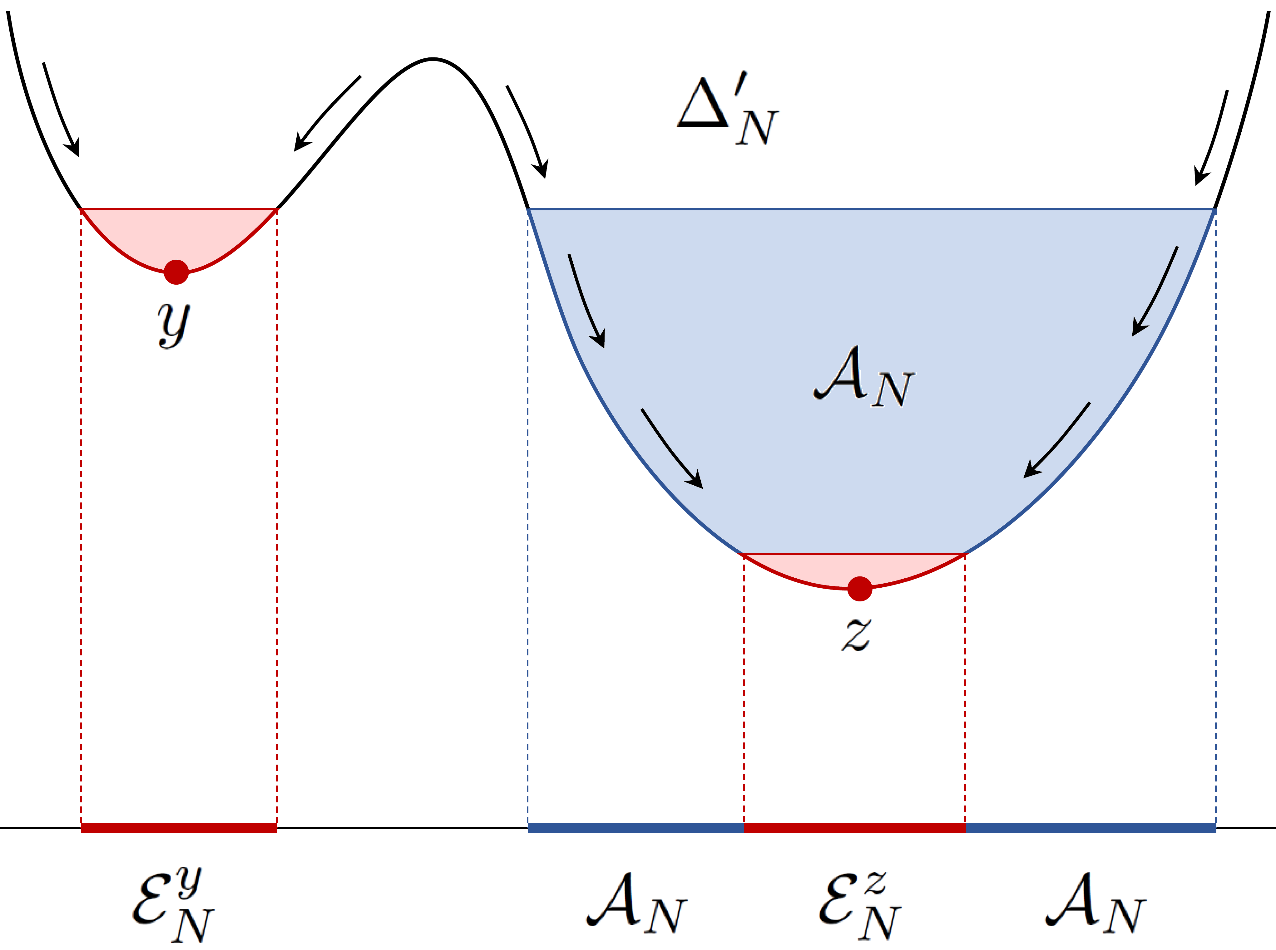
Figure 1. This picture illustrates the idea behind the statement of Lemma 7.4. To simplify, we argue in a continuous setting, but the same idea applies to the discrete setting. Consider a diffusion on the potential field appearing in the picture. The valley ${\mathcal{E}}_{N}^{y}$ is a metastable set and ${\mathcal{E}}_{N}^{z}$ a stable one. As $\mu_{N}(\Delta_{N})/\mu_{N}({\mathcal{E}}_{N}^{y})$ does not converge to $0$, we decompose $\Delta_{N}$ as $\Delta^{\prime}_{N}\cup{\mathcal{A}}_{N}$, so that $\mu_{N}(\Delta^{\prime}_{N})/\mu_{N}({\mathcal{E}}_{N}^{y})\rightarrow 0$. On the other hand, as ${\mathcal{A}}_{N}$ is a subset of the domain of attraction of the valley ${\mathcal{E}}_{N}^{z}$, we can expect (7.5) to hold.

Lemma 7.4.

Fix $y\in S$, and suppose that $\Delta_{N}$ may be decomposed as $\Delta_{N}=\Delta^{\prime}_{N}\cup{\mathcal{A}}_{N}$, $\Delta^{\prime}_{N}\cap{\mathcal{A}}_{N}=\varnothing$, where $\mu_{N}(\Delta^{\prime}_{N})/\mu_{N}({\mathcal{E}}^{y}_{N})\to 0$, and

$$\lim_{N\to\infty}\sup_{\zeta\in{\mathcal{A}}_{N}}{\mathbf{E}}^{N}_{\zeta}\Big{[}\,\int_{0}^{\tau_{\breve{{\mathcal{E}}}_{N}^{y}}}\chi_{{\mathcal{A}}_{N}}(\xi_{N}(s))\,ds\,\Big{]}\;=\;0\;.$$ (7.5)

Then, (7.1) holds for $y$.

Proof.

In equation (7.1), write $\chi_{\Delta_{N}}$ as $\chi_{{\mathcal{A}}_{N}}+\chi_{\Delta^{\prime}_{N}}$. We estimate the two pieces separately. By (7.4) with $\Delta^{\prime}_{N}$ instead of $\Delta_{N}$,

$$\Big{(}\sum_{x\not=y}r_{N}(y,x)\Big{)}\,{\mathbf{E}}^{N}_{\nu^{\dagger}_{y}}\Big{[}\,\int_{0}^{\tau_{\breve{{\mathcal{E}}}_{N}^{y}}}\chi_{\Delta^{\prime}_{N}}(\xi_{N}(s))\,ds\,\Big{]}\;\leq\;\frac{\mu_{N}(\Delta^{\prime}_{N})}{\mu_{N}({\mathscr{E}}^{y}_{N})}\;\cdot$$

By hypothesis, this expression vanishes as $N\to\infty$.

On the other hand, starting the integral from the hitting time of ${\mathcal{A}}_{N}$ and applying the strong Markov property, yields that

$${\mathbf{E}}^{N}_{\nu^{\dagger}_{y}}\Big{[}\,\int_{0}^{\tau_{\breve{{\mathcal{E}}}_{N}^{y}}}\chi_{{\mathcal{A}}_{N}}(\xi_{N}(s))\,ds\,\Big{]} =\;{\mathbf{E}}^{N}_{\nu^{\dagger}_{y}}\Big{[}\,\int_{\tau_{{\mathcal{A}}_{N}}}^{\tau_{\breve{{\mathcal{E}}}_{N}^{y}}}\chi_{{\mathcal{A}}_{N}}(\xi_{N}(s))\,ds\,\Big{]}\;$$

$$\leq\;\sup_{\zeta\in{\mathcal{A}}_{N}}{\mathbf{E}}^{N}_{\zeta}\Big{[}\,\int_{0}^{\tau_{\breve{{\mathcal{E}}}_{N}^{y}}}\chi_{{\mathcal{A}}_{N}}(\xi_{N}(s))\,ds\,\Big{]}\;.$$

By assumption this expression vanishes as $N\to\infty$, which completes the proof of the lemma. ∎

8. Proof of Theorem 3.2

In view of Theorem 2.3, to prove Theorem 3.2, we have to show that conditions ${\mathfrak{D}}$ and ${\mathfrak{R}}_{{\mathscr{L}}}$ hold. The proof of these properties is based on the theory developed in the previous sections. We proceed as follows.

Condition ${\mathfrak{R}}_{{\mathscr{L}}}$. In Proposition 10.1, we show that condition ${\mathfrak{V}}$ is fulfilled. Hence, by Proposition 6.2, property ${\mathfrak{R}}^{(1)}$ holds.

In Corollary 12.2 we show that condition (H0) holds. Since we already proved that condition ${\mathfrak{R}}^{(1)}$ is fulfilled, and since, by Theorem 3.1, $\mu_{N}(\Delta_{N})/\mu_{N}({\mathcal{E}}^{x}_{N})\to 0$ for all $x\in S$, by Corollary 7.3, property ${\mathfrak{R}}^{(2)}_{L_{Y}}$ is in force, where $L_{Y}$ is the generator introduced in (3.7).

Condition ${\mathfrak{D}}$. Recall assumptions (6.3) and (6.4) of condition ${\mathfrak{M}}$. In Corollary 9.2, we show that condition (6.3) holds for some enlarged wells ${\mathcal{V}}^{x}_{N}$ and a time-scale ${\mathbf{h}}_{N}\ll 1$. Then, in Proposition 11.1, we prove that, for every $\epsilon>0$, the mixing time $t^{x}_{\rm mix}(\epsilon)$ of the zero-range process reflected at the boundary of the set ${{\mathcal{V}}}^{x}_{N}$ is bounded by a sequence ${\mathbf{s}}_{N}\ll{\mathbf{h}}_{N}$. This property implies condition (6.4). These two results yield condition ${\mathfrak{M}}$, which is the assertion of Corollary 11.2. Thus, by Theorem 3.1 and Corollary 6.11, property ${\mathfrak{D}}$ is fulfilled.

Remark 8.1.

To deduce property ${\mathfrak{R}}^{(1)}$ one could also invoke Corollary 11.2 and Proposition 6.7. On the other hand, condition ${\mathfrak{R}}^{(2)}_{L_{Y}}$ has been proven in an alternative way in [41, Section 7].

9. Escape from large wells

In this section, we prove that condition (6.3) holds for the critical zero-range process for a sequence $({\mathbf{h}}_{N})_{N\in{\mathbb{N}}}$, ${\mathbf{h}}_{N}\to 0$, and enlarged wells $({\mathcal{V}}_{N}^{x},\,x\in S)_{N\in{\mathbb{N}}}$, ${\mathcal{V}}^{x}_{N}\supset{\mathcal{E}}^{x}_{N}$.

For $N\in{\mathbb{N}}$, set

$$m_{N}=N/(\log N)^{\delta}\text{\; with}\;\;\delta\in(0,\,1)$$

and let ${\mathbf{h}}_{N}$ be the macroscopic time-scales given by

$${\mathbf{h}}_{N}\;:=\;\frac{m_{N}^{2}\,(\log N)^{1/2}}{\theta_{N}}\;=\;\frac{1}{(\log N)^{(1/2)+2\delta}}\;\cdot$$ (9.1)

For $x\in S$, define a larger well by

$${\mathcal{V}}_{N}^{x}\;=\;\{\,\eta\in{\mathcal{H}}_{N}:\eta_{y}\,\leq\,m_{N}\text{ for all }y\in S\setminus\{x\}\,\}\;.$$ (9.2)

As in [41], denote by ${\mathcal{W}}_{N}^{x}$, ${\mathcal{D}}_{N}^{x}$, $x\in S$, the wells given by

$${\mathcal{W}}_{N}^{x}\;=\;\{\,\eta\in{\mathcal{H}}_{N}\,:\,\eta_{x}\,\geq\,N-m_{N}\,\}\;,\quad{\mathcal{D}}_{N}^{x}\;=\;\{\,\eta\in{\mathcal{H}}_{N}\,:\,\eta_{x}\,\geq\,N-N^{\gamma}\,\}\;.$$ (9.3)

In this formula, $\gamma\in(0,\,2/\kappa)$ is a fixed constant. The sets ${\mathcal{D}}_{N}^{x}$ are called deep wells and the sets ${\mathcal{W}}_{N}^{x}$ shallow wells.

Denote by ${\color[rgb]{0,0,1}\zeta_{N}^{x}}\in{\mathcal{H}}_{N}$ the configuration such that all $N$ particles are located at site $x$, so that

$$\zeta_{N}^{x}\,\in\,{\mathcal{D}}_{N}^{x}\,\subset\,{\mathcal{E}}_{N}^{x}\,\subset\,{\mathcal{W}}_{N}^{x}\,\subset\,{\mathcal{V}}_{N}^{x}\;.$$ (9.4)

The main result of this section asserts that the process $\xi_{N}(\cdot)$ starting from a well ${\mathcal{E}}_{N}^{x}$ cannot escape from the well ${\mathcal{W}}_{N}^{x}$ within the time scale ${\mathbf{h}}_{N}$.

Proposition 9.1.

For all $x\in S$,

$$\lim_{N\to\infty}\sup_{\eta\in{\mathcal{E}}_{N}^{x}}{\mathbf{P}}_{\eta}^{N}\,[\,\tau_{({\mathcal{W}}_{N}^{x})^{c}}\leq{\mathbf{h}}_{N}\,]\;=\;0\;.$$

By the last inclusion of (9.4), the next result is a straightforward consequence of Proposition 9.1.

Corollary 9.2.

For all $x\in S$,

$$\lim_{N\rightarrow\infty}\sup_{\eta\in{\mathcal{E}}_{N}^{x}}{\mathbf{P}}_{\eta}^{N}\,[\,\tau_{({\mathcal{V}}_{N}^{x})^{c}}\leq{\mathbf{h}}_{N}\,]\;=\;0\;.$$

9.1. Estimates based on capacity

In this subsection, we state several estimates based on the following bound of the capacity between ${\mathcal{E}}_{N}^{x}$ and $({\mathcal{W}}_{N}^{x})^{c}$ with respect to the critical zero-range processes.

Lemma 9.3.

There exists a finite constant $C$ such that

$$\textup{cap}_{N}({\mathcal{E}}_{N}^{x},\,({\mathcal{W}}_{N}^{x})^{c})\;\leq\;\frac{C\,\theta_{N}}{m_{N}^{2}\log N}$$

for all $x\in S$, $N\geq 1$.

Proof.

Let ${\color[rgb]{0,0,1}Q(\eta)}=q(N-\eta_{x})$ for some function $q:{\mathbb{Z}}\to{\mathbb{R}}$ such that

$$q(k)\;=\;\begin{cases}0&\text{if }k\leq\ell_{N}\;,\\ 1&\text{if }k\geq m_{N}\;.\end{cases}$$

The precise expression for $q$ will be specified below in (9.5). By the Dirichlet principle and since $Q(\sigma^{y,\,z}\eta)=Q(\eta)$ if $y,\,z\neq x$ or $\eta\notin{\mathcal{W}}_{N}^{x}\setminus{\mathcal{E}}_{N}^{x}$,

$$\textup{cap}_{N}({\mathcal{E}}_{N}^{x},\,({\mathcal{W}}_{N}^{x})^{c})$$

$$\qquad\leq\;{\mathscr{D}}_{N}(Q)\;=\;\theta_{N}\,\sum_{\eta\in{\mathcal{W}}_{N}^{x}\setminus{\mathcal{E}}_{N}^{x}}\,\sum_{y\in S}\,\mu_{N}(\eta)\,g(\eta_{x})\,r(x,\,y)\,[\,Q(\sigma^{x,\,y}\eta)\,-\,Q(\eta)\,]^{2}\;.$$

By definition of the jump rates and of $Q$, this expression is bounded by

$$C\,\theta_{N}\,\sum_{\eta\in{\mathcal{W}}_{N}^{x}\setminus{\mathcal{E}}_{N}^{x}}\mu_{N}(\eta)\,[\,q(N-\eta_{x}+1)\,-\,q(N-\eta_{x})\,]^{2}\;,$$

for some finite constant $C$. Let

$${\mathcal{R}}_{k}\;=\;\{\eta\in{\mathcal{H}}_{N}:N-\eta_{x}=k\}$$

so that

$$\textup{cap}_{N}({\mathcal{E}}_{N}^{x},\,({\mathcal{W}}_{N}^{x})^{c})\;\leq\;C\,\theta_{N}\,\sum_{k=\ell_{N}}^{m_{N}-1}\,\mu_{N}({\mathcal{R}}_{k})\,[\,q(k+1)\,-\,q(k)\,]^{2}\;.$$

Define

$$q(k)\;=\;\frac{\sum_{i=\ell_{N}}^{k-1}\,\mu_{N}({\mathcal{R}}_{i})^{-1}}{\sum_{i=\ell_{N}}^{m_{N}-1}\,\mu_{N}({\mathcal{R}}_{i})^{-1}}\;\;\;\;;\;k\,\in\,[\,\ell_{N},\,m_{N}\,]\;.$$ (9.5)

It follows from the penultimate displayed equation that

$$\textup{cap}_{N}({\mathcal{E}}_{N}^{x},\,({\mathcal{W}}_{N}^{x})^{c})\;\leq\;\frac{C\,\theta_{N}}{\sum_{i=\ell_{N}}^{m_{N}-1}\,\mu_{N}({\mathcal{R}}_{i})^{-1}}\;.$$ (9.6)

For $\ell_{N}\leq i<m_{N}$,

$$\mu_{N}({\mathcal{R}}_{i})\;=\;\frac{N}{Z_{N,\,\kappa}\,(\log N)^{\kappa-1}}\,\frac{1}{N-i}\,\frac{Z_{i,\,\kappa-1}\,(\log i)^{\kappa-2}}{i}\;\leq\;\frac{C}{\log N}\,\frac{1}{i}\;\cdot$$

Here, we used the facts that $Z_{N,\,\kappa}$, $Z_{i,\,\kappa-1}$ are bounded, that $N/(N-i)\simeq 1$ and $\log i/\log N\simeq 1$ for $i\in[\ell_{N},\,m_{N}-1]$. Inserting this into (9.6) yields

$$\textup{cap}_{N}({\mathcal{E}}_{N}^{x},\,({\mathcal{W}}_{N}^{x})^{c})\;\leq\;\frac{C\,\theta_{N}}{(\log N)\,\sum_{i=\ell_{N}}^{m_{N}-1}i}\;\leq\;\frac{C\,\theta_{N}}{m_{N}^{2}\,\log N}\;,$$

as claimed. ∎

Based on the previous estimate of the capacity, we can refine [41, Propositions 9.4 and 8.6], replacing the set $\breve{{\mathcal{E}}}_{N}^{x}={\mathcal{E}}_{N}\setminus{\mathcal{E}}_{N}^{x}$ by the much larger set $({\mathcal{W}}_{N}^{x})^{c}$.

Lemma 9.4.

For all $x\in S$,

$$\lim_{N\rightarrow\infty}\,\inf_{\eta\in{\mathcal{D}}_{N}^{x}}\,\inf_{\zeta\in{\mathcal{D}}_{N}^{x}}{\mathbf{P}}_{\eta}^{N}\,[\,\tau_{\zeta}\,<\,\tau_{({\mathcal{W}}_{N}^{x})^{c}}\,]\;=\;1\;.$$

Proof.

By [38, equation (3.3)] and the monotonicity of the capacity,

$${\mathbf{P}}_{\eta}^{N}\,[\,\tau_{\zeta}\,>\,\tau_{({\mathcal{W}}_{N}^{x})^{c}}\,]\;\leq\;\frac{\textup{cap}_{N}(\eta,\,({\mathcal{W}}_{N}^{x})^{c})}{\textup{cap}_{N}(\eta,\,\zeta)}\;\leq\;\frac{\textup{cap}_{N}({\mathcal{E}}_{N}^{x},\,({\mathcal{W}}_{N}^{x})^{c})}{\textup{cap}_{N}(\eta,\,\zeta)}\;.$$

Hence, by [41, Lemma 9.3] and Lemma 9.3,

$${\mathbf{P}}_{\eta}^{N}\,[\,\tau_{\zeta}\,>\,\tau_{({\mathcal{W}}_{N}^{x})^{c}}\,]\;\leq\;C\,\frac{N^{\gamma\kappa}\,(\log N)^{\kappa-1}}{m_{N}^{2}\,\log N}\;=\;o_{N}(1)\;,$$

where the last equality holds because $\gamma<2/\kappa$. This completes the proof. ∎

Recall from [41, Proposition 9.1] that the deep wells ${\mathcal{D}}_{N}^{x}$ are attractors, in the sense that

$$\lim\limits_{N\rightarrow\infty}\inf\limits_{\eta\in{\mathcal{E}}_{N}^{x}}{\mathbf{P}}_{\eta}^{N}[\,\tau_{{\mathcal{D}}_{N}^{x}}\,<\,\tau_{({\mathcal{W}}_{N}^{x})^{c}}\,]\;=\;1\;\;\;\;\text{for all}\;x\in S\;.$$ (9.7)

Lemma 9.5.

For all $x\in S$,

$$\lim_{N\rightarrow\infty}\,\inf_{\zeta\in{\mathcal{D}}_{N}^{x}}\,\inf_{\eta\in{\mathcal{E}}_{N}^{x}}{\mathbf{P}}_{\eta}^{N}\,[\,\tau_{\zeta}\,<\,\tau_{({\mathcal{W}}_{N}^{x})^{c}}\,]\;=\;1\;.$$

Proof.

Fix $x\in S$, $\eta\in{\mathcal{E}}_{N}^{x}$, and $\zeta\in{\mathcal{D}}_{N}^{x}$. Then, by the strong Markov property,

$${\mathbf{P}}_{\eta}^{N}[\,\tau_{\zeta}\,<\,\tau_{({\mathcal{W}}_{N}^{x})^{c}}\,]\; \geq\;{\mathbf{P}}_{\eta}^{N}\,[\,\tau_{\zeta}\,<\,\tau_{({\mathcal{W}}_{N}^{x})^{c}}\,,\;\tau_{{\mathcal{D}}_{N}^{x}}\,<\,\tau_{({\mathcal{W}}_{N}^{x})^{c}}\,]$$

$$\geq\;{\mathbf{P}}_{\eta}^{N}\,[\,\tau_{{\mathcal{D}}_{N}^{x}}\,<\,\tau_{({\mathcal{W}}_{N}^{x})^{c}}\,]\,\inf_{\xi\in{\mathcal{D}}_{N}^{x}}{\mathbf{P}}_{\xi}^{N}\,[\,\tau_{\zeta}\,<\,\tau_{({\mathcal{W}}_{N}^{x})^{c}}\,]\;.$$

Therefore, we have

$$\inf_{\zeta\in{\mathcal{D}}_{N}^{x}}\,\inf_{\eta\in{\mathcal{E}}_{N}^{x}}{\mathbf{P}}_{\eta}^{N}\,[\,\tau_{\zeta}\,<\,\tau_{({\mathcal{W}}_{N}^{x})^{c}}\,]$$

$$\geq\; \inf_{\eta\in{\mathcal{E}}_{N}^{x}}{\mathbf{P}}_{\eta}^{N}\,[\,\tau_{{\mathcal{D}}_{N}^{x}}\,<\,\tau_{({\mathcal{W}}_{N}^{x})^{c}}\,]\,\times\,\inf_{\zeta\in{\mathcal{D}}_{N}^{x}}\,\inf_{\xi\in{\mathcal{D}}_{N}^{x}}{\mathbf{P}}_{\xi}^{N}\,[\,\tau_{\zeta}\,<\,\tau_{({\mathcal{W}}_{N}^{x})^{c}}\,]\;.$$

The first term at the right-hand side is $1-o_{N}(1)$ by (9.7), and the second one is $1-o_{N}(1)$ by Lemma 9.4. This completes the proof of the lemma. ∎

9.2. Proof of Proposition 9.1

The proof of Proposition 9.1 is similar to the one of [41, Theorem 3.2]. First, we establish the following estimate, whose proof is omitted since it is completely identical to the proof of [41, Proposition 8.4]. It suffices to replace $\breve{{\mathcal{E}}}_{N}^{x}$ by $({\mathcal{W}}_{N}^{x})^{c}$ and $1/\gamma_{N}$ by $t_{N}$.

Lemma 9.6.

For all $x\in S$ and probability measure $\upsilon_{N}$ concentrated on ${\mathcal{E}}_{N}^{x}$,

$$\big{(}\,{\mathbf{P}}_{\upsilon_{N}}^{N}\,[\,\tau_{({\mathcal{W}}_{N}^{x})^{c}}\,\leq\,{\mathbf{h}}_{N}\,]\,\big{)}\,^{2}\;\leq\;e^{2}\,{\mathbf{h}}_{N}\,{\mathbb{E}}_{\mu_{N}^{x}}\,\bigg{[}\,\bigg{(}\,\frac{\upsilon_{N}}{\mu_{N}^{x}}\,\bigg{)}^{2}\,\bigg{]}\,\frac{1}{\mu_{N}({\mathcal{E}}_{N}^{x})}\,\textup{cap}_{N}({\mathcal{E}}_{N}^{x},\,({\mathcal{W}}_{N}^{x})^{c})\;.$$

By inserting $\upsilon_{N}={\color[rgb]{0,0,1}\pi_{N}^{x}(\cdot)}\coloneqq\mu_{N}(\,\cdot\,|\,{\mathcal{D}}_{N}^{x})$ into the previous equation, we obtain the following estimate. The order of magnitude of ${\mathbf{h}}_{N}$ is critically used in the proof of this result.

Lemma 9.7.

For all $x\in S$,

$$\lim_{N\to\infty}{\mathbf{P}}_{\pi_{N}^{x}}^{N}\,[\,\tau_{({\mathcal{W}}_{N}^{x})^{c}}\,\leq\,{\mathbf{h}}_{N}\,]\;=\;0\;.$$

Proof.

Since

$${\mathbb{E}}_{\mu_{N}^{x}}\,\Big{[}\,\Big{(}\,\frac{\upsilon_{N}}{\mu_{N}^{x}}\,\Big{)}\,\Big{]}^{2}\;=\;\frac{\mu_{N}({\mathcal{E}}_{N}^{x})}{\mu_{N}({\mathcal{D}}_{N}^{x})}\;,$$

by Lemmata 9.3 and 9.6, we get

$$\big{(}\,{\mathbf{P}}_{\upsilon_{N}}^{N}\,[\,\tau_{({\mathcal{W}}_{N}^{x})^{c}}\leq{\mathbf{h}}_{N}\,]\,\big{)}\,^{2}\;\leq\;C\,{\mathbf{h}}_{N}\,\frac{1}{\mu_{N}({\mathcal{D}}_{N}^{x})}\,\frac{\theta_{N}}{m_{N}^{2}\log N}\;=\;\frac{C}{(\log N)^{1/2}}\,\frac{1}{\mu_{N}({\mathcal{D}}_{N}^{x})}\;\cdot$$

By [41, Lemma 4.2], $\mu_{N}({\mathcal{D}}_{N}^{x})\simeq\frac{1}{\kappa}\gamma^{\kappa-1}$, which completes the proof. ∎

Proof of Proposition 9.1.

Fix $\eta\in{\mathcal{E}}_{N}^{x}$ and $\zeta\in{\mathcal{D}}_{N}^{x}$. By Lemma 9.5,

$${\mathbf{P}}_{\eta}^{N}\,[\,\tau_{({\mathcal{W}}_{N}^{x})^{c}}\leq{\mathbf{h}}_{N}\,]\; \leq\;{\mathbf{P}}_{\eta}^{N}\,[\,\tau_{({\mathcal{W}}_{N}^{x})^{c}}\,\leq\,{\mathbf{h}}_{N}\,,\,\,\tau_{\zeta}\,<\,\tau_{({\mathcal{W}}_{N}^{x})^{c}}\,]\,+\,{\mathbf{P}}_{\eta}^{N}\,[\,\tau_{\zeta}\,>\,\tau_{({\mathcal{W}}_{N}^{x})^{c}}\,]\,$$

$$=\;{\mathbf{P}}_{\eta}^{N}\,[\,\tau_{({\mathcal{W}}_{N}^{x})^{c}}\,\leq\,{\mathbf{h}}_{N}\,,\,\,\tau_{\zeta}\,<\,\tau_{({\mathcal{W}}_{N}^{x})^{c}}\,]\,+\,o_{N}(1)\;.$$

By the strong Markov property,

$${\mathbf{P}}_{\eta}^{N}\,[\,\tau_{({\mathcal{W}}_{N}^{x})^{c}}\,\leq\,{\mathbf{h}}_{N}\,,\;\tau_{\zeta}\,<\,\tau_{({\mathcal{W}}_{N}^{x})^{c}}\,]\;\leq\;{\mathbf{P}}_{\zeta}^{N}\,[\,\tau_{({\mathcal{W}}_{N}^{x})^{c}}\,\leq\,{\mathbf{h}}_{N}\,]\,$$

so that

$${\mathbf{P}}_{\eta}^{N}\,[\,\tau_{({\mathcal{W}}_{N}^{x})^{c}}\,\leq\,{\mathbf{h}}_{N}\,]\;\leq\;{\mathbf{P}}_{\zeta}^{N}\,[\,\tau_{({\mathcal{W}}_{N}^{x})^{c}}\,\leq\,{\mathbf{h}}_{N}\,]\,+\,o_{N}(1)\;.$$

Multiplying both sides by $\pi_{N}^{x}(\zeta)$ and summing over $\zeta\in{\mathcal{D}}_{N}^{x}$, we get

$${\mathbf{P}}_{\eta}^{N}\,[\,\tau_{({\mathcal{W}}_{N}^{x})^{c}}\,\leq\,{\mathbf{h}}_{N}\,]\;\leq\;{\mathbf{P}}_{\pi_{N}^{x}}^{N}\,[\,\tau_{({\mathcal{W}}_{N}^{x})^{c}}\,\leq\,{\mathbf{h}}_{N}\,]\,+\,o_{N}(1)\;.$$

Apply Lemma 9.7 to complete the proof. ∎

10. Condition ${\mathfrak{V}}$ for critical zero-range processes

In this section, we prove that the process $\xi_{N}(\cdot)$ starting from a well ${\mathcal{E}}_{N}^{x}$ hits quickly the configuration $\zeta_{N}^{x}$. For $N\geq 1$, define the time scale ${\mathbf{u}}_{N}$ by

$${\mathbf{u}}_{N}\;:=\;\frac{m_{N}^{2}}{\theta_{N}}\;=\;\frac{1}{(\log N)^{1+2\delta}}\;.$$

Proposition 10.1.

For all $x\in S$,

$$\lim_{N\to\infty}\sup_{\eta\in{\mathcal{E}}_{N}^{x}}{\mathbf{P}}_{\eta}^{N}\,[\,\tau_{\zeta_{N}^{x}}\geq{\mathbf{u}}_{N}\,]\;=\;0\;.$$

In particular, the condition ${\mathfrak{V}}$ holds for the critical zero-range processes.

This result is crucially used in the next section to verify the requirement (6.4) of condition ${\mathfrak{M}}$.

10.1. A super-harmonic function

We first establish, in Lemma 10.6 below, the estimate stated in Proposition 10.1 for the process which is reflected at the boundary of ${\mathcal{W}}_{N}^{x}$. The proof of Lemma 10.6 is based on the construction, carried out in [41, Section 10], of a function $G_{N}^{x}:{\mathcal{H}}_{N}\rightarrow{\mathbb{R}}$, $x\in S$, which is super-harmonic on ${\mathcal{W}}_{N}^{x}\setminus{\mathcal{D}}_{N}^{x}$. For the sake of completeness, we recall its definition and main properties below.

Fix $x_{0}\in S$, and let $S_{0}=S\setminus\{x_{0}\}$. For a subset ${\mathcal{C}}$ of ${\mathcal{H}}_{N}$, let

$$\text{int}\,{\mathcal{C}}\;=\;\{\,\eta\in{\mathcal{C}}:\sigma^{x,\,y}\eta\in{\mathcal{C}}\text{ for all }x,\,y\text{ with }r(x,\,y)>0\,\}\;,$$

$$\partial{\mathcal{C}}\;=\;{\mathcal{C}}\setminus\text{int }{\mathcal{C}}\;,$$

$$\overline{{\mathcal{C}}}\;=\;\{\eta\in{\mathcal{H}}_{N}:\eta\in{\mathcal{C}}\text{ or }\sigma^{x,\,y}\eta\in{\mathcal{C}}\text{ for some }x,\,y\text{ with }r(x,\,y)>0\}\;.$$

With this notation, let

$${\mathcal{U}}_{N}^{x_{0}}\;=\;\overline{{\mathcal{W}}_{N}^{x_{0}}\setminus{\mathcal{D}}_{N}^{x_{0}}}\quad\text{so that}\quad\text{int}\,{\mathcal{U}}_{N}^{x_{0}}={\mathcal{W}}_{N}^{x_{0}}\setminus{\mathcal{D}}_{N}^{x_{0}}\;.$$

Recall, from (3.5), that $h_{A,\,B}(\cdot)$ and $\textup{cap}_{X}(\cdot,\,\cdot)$ represent the equilibrium potential and the capacity, respectively, associated to the underlying random walk $X$. For each non-empty subset $A$ of $S_{0}$, consider the sequence $(b_{x,\,y}^{A})_{x,\,y\in S}$ defined by

$$b_{x,\,y}^{A}\;=\;\frac{1}{\kappa}\,\frac{h_{x,\,A^{c}}(y)}{\textup{cap}_{X}(x,\,A^{c})}\;,\quad x\;,y\,\in\,A\;,$$

and $b_{x,\,y}^{A}=0$ otherwise. By elementary properties of the capacity and the equilibrium potential, $b_{x,\,y}^{A}=b_{y,\,x}^{A}$ for all $x,\,y\in S$ (cf. [41, Lemma 10.2]). Moreover, by [41, Lemma 10.3],

$$b_{x,\,y}^{A}\leq b_{x,\,y}^{B}\;\;\text{for all }x,\,y\in S$$ (10.1)

if $A\subset B\subset S_{0}$.

For each non-empty subset $A$ of $S_{0}$, define the quadratic function $P^{A}(\cdot)$ as

$$P^{A}(\eta)\;=\;\frac{1}{2}\,\sum_{x\in A}b_{x,\,x}^{A}\,\eta_{x}\,(\eta_{x}-1)\;+\;\sum_{\{x,\,y\}\subset A}b_{x,\,y}^{A}\,\eta_{x}\,\eta_{y}\;.$$

By [41, Lemma 10.8],

$$c_{1}\,\Big{(}\sum_{x\in S_{0}}\eta_{x}\Big{)}^{2}\;\leq\;P^{S_{0}}(\eta)\;\leq\;c_{2}\,\Big{(}\sum_{x\in S_{0}}\eta_{x}\Big{)}^{2}\;.$$ (10.2)

Fix $A\subsetneq S_{0}$. For each constant $c_{A}>0$ and positive integer $\ell\geq 1$, let $P_{\ell}^{A}:{\mathcal{U}}_{N}^{x_{0}}\rightarrow{\mathbb{R}}$ be given by

$$P_{\ell}^{A}(\eta)\;=\;P^{A}(\eta)\;-\;c_{A}\,\ell^{2}\;.$$

The dependence of $P_{\ell}^{A}$ on the constant $c_{A}$ is omitted from the notation. Taking $P_{\ell}^{\varnothing}(\eta)=0$ for all $\eta\in{\mathcal{U}}_{N}^{x_{0}}$, define the corrector function $W_{\ell}:{\mathcal{U}}_{N}^{x_{0}}\rightarrow{\mathbb{R}}$ by

$$W_{\ell}(\eta)=\min\left\{P_{\ell}^{A}(\eta):A\subset S_{0}\,,\,A\not=S_{0}\,\right\}\;.$$

By [41, Lemma 10.10], there exists a constant $0<C<\infty$ such that

$$-\,C\,\ell^{2}\leq W_{\ell}(\eta)\leq 0\;.$$

Hence, by (10.2) and the previous bound, $P^{S_{0}}(\eta)-W_{\ell}(\eta)>0$ for all $\eta\in{\mathcal{U}}_{N}^{x_{0}}$.

For each positive integer $m>2$, define the function $G_{N}^{x_{0}}:{\mathcal{H}}_{N}\rightarrow{\mathbb{R}}$ by

$$G_{N}^{x_{0}}(\eta)\;=\;\begin{cases}{\displaystyle\sum_{\ell=2}^{m}\frac{1}{\ell}\,[\,P^{S_{0}}(\eta)\,-\,W_{\ell}(\eta)\,]^{1/2}\;,}&\eta\,\in\,{\mathcal{U}}_{N}^{x_{0}}\;,\\ \vphantom{\Big{\{}}0\;,&\zeta\,\in\,{\mathcal{H}}_{N}\setminus{\mathcal{U}}_{N}^{x_{0}}\;.\end{cases}$$ (10.3)

Here, again, the dependence of $G_{N}^{x_{0}}$ on $m$ is omitted. The next result is [41, Theorem 9.2]. Recall that ${\mathscr{L}}_{N}^{\xi}=\theta_{N}{\mathscr{L}}_{N}$, introduced in Subsection 3.2, is the generator of the speeded-up process.

Theorem 10.2.

For large enough $m$ and a suitable selection of constants $(c_{A})_{A\subsetneq S_{0}}$, the function $G_{N}^{x_{0}}$ is super-harmonic in ${\mathcal{W}}_{N}^{x_{0}}\setminus{\mathcal{D}}_{N}^{x_{0}}$. More precisely, there exists a positive constant $C>0$ such that

$$({\mathscr{L}}_{N}^{\xi}\,G_{N}^{x_{0}})(\eta)\;\leq\;-\frac{C\,\theta_{N}}{N-\eta_{x_{0}}}\text{\;\;\;\;for all }\eta\,\in\,{\mathcal{W}}_{N}^{x_{0}}\setminus{\mathcal{D}}_{N}^{x_{0}}\;.$$

Additionally, there exist constants $0<c_{1}<c_{2}<\infty$ such that

$$c_{1}\,(N-\eta_{x_{0}})\;\leq\;G_{N}^{x_{0}}(\eta)\;\leq\;c_{2}\,(N-\eta_{x_{0}})$$ (10.4)

for all $\eta\,\in\,{\mathcal{W}}_{N}^{x_{0}}\setminus{\mathcal{D}}_{N}^{x_{0}}$.

10.2. Reflected processes

Denote by ${\color[rgb]{0,0,1}(\widehat{\xi}_{N}^{x}(t))_{t\geq 0}}$ the continuous-time Markov chain on ${\mathcal{W}}_{N}^{x}$ obtained by reflecting the zero-range process $\xi_{N}(\cdot)$ at the boundary of this set. In other words, the process $\widehat{\xi}_{N}^{x}(\cdot)$ behaves as the zero-range process inside the well ${\mathcal{W}}_{N}^{x}$, but its jumps to the set $({\mathcal{W}}_{N}^{x})^{c}$ are suppressed. Denote by $\widehat{{\mathbf{P}}}_{\eta}^{N,\,x}$ the law of the reflected process $\widehat{\xi}_{N}^{x}(\cdot)$, and by $\widehat{{\mathbf{E}}}_{\eta}^{N,\,x}$ the expectation with respect to $\widehat{{\mathbf{P}}}_{\eta}^{N,\,x}$.

The next result asserts that the function $G_{N}^{x_{0}}$ is also super-harmonic at ${\mathcal{W}}_{N}^{x_{0}}\setminus{\mathcal{D}}_{N}^{x_{0}}$ for the reflected process. Denote by ${\color[rgb]{0,0,1}{\mathscr{L}}_{N}^{x_{0}}}$ the generator associated to the reflected process $\widehat{\xi}_{N}^{x_{0}}(\cdot)$.

Lemma 10.3.

Fix $x_{0}\in S$, and let $G_{N}^{x_{0}}$ be the function given by (10.3). Then, there exists $C>0$ such that

$$({\mathscr{L}}_{N}^{x_{0}}\,G_{N}^{x_{0}})(\eta)\;\leq\;-\frac{C\,\theta_{N}}{N-\eta_{x_{0}}}\text{\;\;\;\;for all }\eta\,\in\,{\mathcal{W}}_{N}^{x_{0}}\setminus{\mathcal{D}}_{N}^{x_{0}}\;.$$

The main difference between this lemma and Theorem 10.2 is the analysis around the boundary of ${\mathcal{W}}_{N}^{x_{0}}$, since the generator ${\mathscr{L}}_{N}^{x_{0}}$ differs from ${\mathscr{L}}_{N}$ there, as the jumps to set $({\mathcal{W}}_{N}^{x_{0}})^{c}$ are excluded.

Proof.

Since we possibly have $({\mathscr{L}}_{N}^{x_{0}}G_{N}^{x_{0}})(\eta)\neq({\mathscr{L}}_{N}G_{N}^{x_{0}})(\eta)$ only at the boundary ${\color[rgb]{0,0,1}\partial{\mathcal{W}}_{N}^{x_{0}}}=\{\eta:\eta_{x_{0}}=N-m_{N}\}$, it suffices to show that

$$({{\mathscr{L}}}_{N}^{x_{0}}\,G_{N}^{x_{0}})(\eta)\;\leq\;({{\mathscr{L}}}_{N}^{\xi}\,G_{N}^{x_{0}})(\eta)\text{\;\;\;\; for all }\eta\in\partial{\mathcal{W}}_{N}^{x_{0}}\;.$$

At $\partial{\mathcal{W}}_{N}^{x_{0}}$, the reflected process cannot decrease the number of particles at site $x_{0}$. Thus,

$$({{\mathscr{L}}}_{N}^{x_{0}}\,G_{N}^{x_{0}})(\eta)\;=\;({{\mathscr{L}}}_{N}^{\xi}\,G_{N}^{x_{0}})(\eta)\,-\,\theta_{N}\,\sum_{y\in S}g(\eta_{x_{0}})\,r(x_{0},\,y)\,[\,G_{N}^{x_{0}}(\sigma^{x_{0},\,y}\eta)\,-\,G_{N}^{x_{0}}(\eta)\,]\;,$$

and it is enough to show that

$$G_{N}^{x_{0}}(\sigma^{x_{0},\,y}\eta)\;\geq\;G_{N}^{x_{0}}(\eta)\text{ \;\;\;\;for all }\eta\,\in\,\partial{\mathcal{W}}_{N}^{x_{0}}\;.$$

Actually, by the definition (10.3) of $G_{N}^{x_{0}}$, it is enough to show that

$$P^{S_{0}}(\sigma^{x_{0},\,y}\eta)\,-\,W_{\ell}(\sigma^{x_{0},\,y}\eta)\;\geq\;P^{S_{0}}(\eta)\,-\,W_{\ell}(\eta)$$ (10.5)

for all $\ell\geq 2$ and $\eta\,\in\,\partial{\mathcal{W}}_{N}^{x_{0}}$.

Fix $A\subsetneq S_{0}$, by definitions of $P^{S_{0}}$ and $P^{A}$ along with the increasing property (10.1),

$$P^{S_{0}}(\sigma^{x_{0},\,y}\eta)\,-\,P^{S_{0}}(\eta)\;=\;\sum_{z\in S_{0}}b_{y,\,z}^{S_{0}}\,\eta_{z}\;\geq\;\sum_{z\in A}b_{y,\,z}^{A}\,\eta_{z}\;=\;P^{A}(\sigma^{x_{0},\,y}\eta)\,-\,P^{A}(\eta)\;.$$ (10.6)

Hence, if $W_{\ell}(\eta)=P_{\ell}^{A}(\eta)$ and $W_{\ell}(\sigma^{x,\,y}\eta)=P_{\ell}^{A}(\sigma^{x,\,y}\eta)$ for the same set $A\subsetneq S\setminus\{x_{0}\}$, (10.5) follows from (10.6).

On the other hand, if $W_{\ell}(\eta)=P_{\ell}^{A}(\eta)$ and $W_{\ell}(\sigma^{x,\,y}\eta)=P_{\ell}^{B}(\sigma^{x,\,y}\eta)$ for some $A\neq B$, by definition of $W_{\ell}$ and (10.6),

$$W_{\ell}(\sigma^{x,\,y}\eta)\,-\,W_{\ell}(\eta) \;=\;P_{\ell}^{B}(\sigma^{x,y}\eta)\,-\,P_{\ell}^{A}(\eta)$$

$$\leq\;P_{\ell}^{A}(\sigma^{x,y}\eta)\,-\,P_{\ell}^{A}(\eta)\;\leq\;P(\sigma^{x,y}\eta)\,-\,P(\eta)\;.$$

This completes the proof of (10.5), and the one of the lemma. ∎

10.3. Hitting times of the reflected process

In this subsection, we establish, in Lemma 10.6 below, that the assertion of Proposition 10.1 holds for the reflected process $\widehat{\xi}_{N}^{x}(\cdot)$. The first result asserts that the process $\widehat{\xi}_{N}^{x}(\cdot)$ hits the set ${\mathcal{D}}_{N}^{x}$ quickly when it starts from a configuration in ${\mathcal{E}}_{N}^{x}$.

Lemma 10.4.

There exists $C>0$ such that, for all $x\in S$, $N\geq 1$,

$$\sup_{\eta\in{\mathcal{E}}_{N}^{x}}\widehat{{\mathbf{E}}}_{\eta}^{N,\,x}\,[\,\tau_{{\mathcal{D}}_{N}^{x}}\,]\;\leq\;C\,\frac{m_{N}\,\ell_{N}}{\theta_{N}}\;\cdot$$

Proof.

By the martingale formulation, for every $t>0$,

$$\widehat{{\mathbf{E}}}_{\eta}^{N,\,x}\,[\,G_{N}^{x}(\,\widehat{\eta}_{N}^{x}(\tau_{{\mathcal{D}}_{N}^{x}}\wedge t)\,)\,]\;=\;G_{N}^{x}(\eta)\,+\,\widehat{{\mathbf{E}}}_{\eta}^{N,\,x}\,\Big{[}\,\int_{0}^{\tau_{{\mathcal{D}}_{N}^{x}}\wedge t}({\mathscr{L}}_{N}^{x}G_{N}^{x})(\widehat{\eta}_{N}^{x}(s))ds\,\Big{]}\;.$$

By Lemma 10.3, there exists a positive constant $C$, whose value may change from line to line, such that

$$({\mathscr{L}}_{N}^{x}\,G_{N}^{x})(\eta)\;\leq\;-\,\frac{C\,\theta_{N}}{N-\eta_{x}}\;\leq\;-\,\frac{C\,\theta_{N}}{m_{N}}\;\;\;\;\text{for }\eta\,\in\,{\mathcal{W}}_{N}^{x}\;.$$

On the other hand, by (10.4), $G_{N}^{x}$ is non-negative. Therefore, by the next to last displayed equation,

$$\frac{C\,\theta_{N}}{m_{N}}\,\widehat{{\mathbf{E}}}_{\eta}^{N,\,x}\,[\,\tau_{{\mathcal{D}}_{N}^{x}}\wedge t\,]\;\leq\;G_{N}^{x}(\eta)\;.$$

By (10.4), there exist a finite constant $C_{1}$ such that $G_{N}^{x}(\eta)\leq C_{1}\,(N-\eta_{x})$. Hence, since $N-\eta_{x}\leq\ell_{N}$ for $\eta\in{\mathcal{E}}_{N}^{x}$,

$$\frac{C\,\theta_{N}}{m_{N}}\,\widehat{{\mathbf{E}}}_{\eta}^{N,\,x}\,[\,\tau_{{\mathcal{D}}_{N}^{x}}\wedge t\,]\;\leq\;C_{1}\,\ell_{N}\;.$$

To complete the proof of the lemma, it remains to let $t\to\infty$. ∎

The next result asserts that $\widehat{\xi}_{N}^{x}(\cdot)$ hits the configuration $\zeta_{N}^{x}$ quickly when it starts from a configuration in ${\mathcal{D}}_{N}^{x}$.

Lemma 10.5.

There exists a finite constant $C$ such that,

$$\sup_{\eta\in{\mathcal{D}}_{N}^{x}}\,\widehat{{\mathbf{E}}}_{\eta}^{N,\,x}\,[\,\tau_{\zeta_{N}^{x}}\,]\;\leq\;C\,\frac{N^{\gamma\kappa}\,(\log N)^{\kappa-1}}{\theta_{N}}$$

for all $x\in S$ and $N\geq 1$.

Proof.

If $\eta=\zeta_{N}^{x}$, there is nothing to prove. For $\eta\neq\zeta_{N}^{x}$, we recall the well-known identity (cf. [6, Proposition 6.10])

$$\widehat{{\mathbf{E}}}_{\eta}^{N,\,x}\,[\,\tau_{\zeta_{N}^{x}}\,]\;=\;\frac{{\mathbb{E}}_{\widehat{\mu}_{N}^{x}}\,[\,{\mathfrak{h}}_{\eta,\,\zeta_{N}^{x}}^{N,\,x}\,]}{\textrm{cap}_{N}^{x}(\eta,\,\zeta_{N}^{x})}\;,$$ (10.7)

where ${\mathfrak{h}}_{\eta,\,\zeta_{N}^{x}}^{N,\,x}$ and $\textrm{cap}_{N}^{x}(\eta,\,\zeta_{N}^{x})$ denote the equilibrium potential and the capacity between $\eta$ and $\zeta_{N}^{x}$ with respect to the reflected process $\widehat{\xi}_{N}^{x}(\cdot)$, respectively, and where $\widehat{\mu}_{N}^{x}(\cdot)$ denotes the invariant measure conditioned on ${\mathcal{W}}_{N}^{x}$, i.e.,

$$\widehat{\mu}_{N}^{x}(\cdot)\;=\;\mu_{N}(\cdot\,|{\mathcal{W}}_{N}^{x})\;=\;\frac{\mu_{N}(\cdot)}{\mu_{N}({\mathcal{W}}_{N}^{x})}\;.$$

Observe that $\widehat{\mu}_{N}^{x}(\cdot)$ is the invariant measure of the reflected process $\widehat{\xi}_{N}^{x}(\cdot)$.

Applying the trivial bound ${\mathfrak{h}}_{\eta,\,\zeta_{N}^{x}}^{N,\,x}\leq 1$ to (10.7), we get

$$\widehat{{\mathbf{E}}}_{\eta}^{N,\,x}\,[\,\tau_{\zeta_{N}^{x}}\,]\;\leq\;\frac{1}{\textrm{cap}_{N}^{x}(\eta,\,\zeta_{N}^{x})}\;\cdot$$

By [41, Lemma 9.3],

$$\textrm{cap}_{N}^{x}(\eta,\,\zeta_{N}^{x})\;\geq\;\frac{C\,\theta_{N}}{N^{\gamma\kappa}\,(\log N)^{\kappa-1}}\;\cdot$$

Actually, in [41, Lemma 9.3] this bound is proved for the capacity with respect to the original zero-range process, but the same proof applies to the reflected process. To complete the proof, it remains to combine the previous bounds. ∎

Lemma 10.6.

For all $x\in S$,

$$\lim_{N\to\infty}\sup_{\eta\in{\mathcal{E}}_{N}^{x}}\widehat{{\mathbf{P}}}_{\eta}^{N,\,x}\,[\,\tau_{\zeta_{N}^{x}}\geq{\mathbf{u}}_{N}\,]\;=\;0\;.$$

Proof.

By Lemmata 10.4, 10.5, and the strong Markov property,

$$\widehat{{\mathbf{E}}}_{\eta}^{N,\,x}\,[\,\tau_{\zeta_{N}^{x}}\,]\;\leq\;\frac{C}{\theta_{N}}\,\Big{\{}\,m_{N}\,\ell_{N}+C\,N^{\gamma\kappa}\,(\log N)^{\kappa-1}\Big{\}}\;\ll\;\frac{m_{N}^{2}}{\theta_{N}}\;,$$

since we assumed that $\gamma<2/\kappa$. The assertion of the lemma follows from Chebyshev inequality. ∎

10.4. Proof of Proposition 10.1

Consider the canonical coupling of the zero-range process $\xi_{N}(\cdot)$ and the reflected process $\widehat{\xi}_{N}^{x}(\cdot)$ starting together at $\eta\in{\mathcal{W}}_{N}^{x}$. The two processes move together until $\xi_{N}(\cdot)$ hits $({\mathcal{W}}_{N}^{x})^{c}$. From this point on, they move independently according to their respective dynamics. By Proposition 9.1, starting from ${\mathcal{E}}_{N}^{x}$, we can couple the original zero-range process and the reflected process $\widehat{\xi}_{N}^{x}(\cdot)$ up to time ${\mathbf{h}}_{N}$ with a probability close to $1$.

The joint law of $\xi_{N}(\cdot)$ and $\widehat{\xi}_{N}^{x}(\cdot)$ under this canonical coupling is represented by $\widehat{\bf{P}}_{\eta}^{N,\,x}$. Denote by $\tau_{{\mathcal{A}}}$ and $\widehat{\tau}_{{\mathcal{A}}}$ the hitting time of a set ${\mathcal{A}}$ with respect to $\xi_{N}(\cdot)$ and $\widehat{\xi}_{N}^{x}(\cdot)$, respectively.

Proof of Proposition 10.1.

Recall the definition of the sequence ${\mathbf{u}}_{N}$ introduced at the beginning of Section 10, and the one of ${\mathbf{h}}_{N}$ presented in (9.1). Fix $\eta\in{\mathcal{E}}_{N}^{x}$. By Proposition 9.1,

$${\mathbf{P}}_{\eta}^{N}\,[\,\tau_{\zeta_{N}^{x}}\,\geq\,{\mathbf{u}}_{N}\,]\;=\;{\mathbf{P}}_{\eta}^{N}\,[\,\tau_{\zeta_{N}^{x}}\,\geq\,{\mathbf{u}}_{N}\,,\,\,\tau_{({\mathcal{W}}_{N}^{x})^{c}}\,>\,{\mathbf{h}}_{N}\,]\,+\,o_{N}(1)\;.$$

Recall the canonical coupling introduced above. On the event $\{\tau_{({\mathcal{W}}_{N}^{x})^{c}}>{\mathbf{h}}_{N}\}$, the two processes $\xi_{N}(t)$ and $\widehat{\xi}_{N}^{x}(t)$ move together until ${\mathbf{h}}_{N}$. Since ${\mathbf{u}}_{N}\ll{\mathbf{h}}_{N}$, on the previous event, the sets $\{\tau_{\zeta_{N}^{x}}\geq{\mathbf{u}}_{N}\}$ and $\{\widehat{\tau}_{\zeta_{N}^{x}}\geq{\mathbf{u}}_{N}\}$ coincide. Thus,

$${\mathbf{P}}_{\eta}^{N}\,[\,\tau_{\zeta_{N}^{x}}\,\geq\,{\mathbf{u}}_{N}\,,\,\,\tau_{({\mathcal{W}}_{N}^{x})^{c}}\,>\,{\mathbf{h}}_{N}\,]\;=\; \widehat{\bf{P}}_{\eta}^{N,\,x}\,[\,\tau_{\zeta_{N}^{x}}\,\geq\,{\mathbf{u}}_{N}\,,\,\,\tau_{({\mathcal{W}}_{N}^{x})^{c}}\,>\,{\mathbf{h}}_{N}\,]$$

$$=\; \widehat{\bf{P}}_{\eta}^{N,\,x}\,[\,\widehat{\tau}_{\zeta_{N}^{x}}\,\geq\,{\mathbf{u}}_{N},\,\tau_{({\mathcal{W}}_{N}^{x})^{c}}\,>\,{\mathbf{h}}_{N}\,]\;.$$

Since,

$$\widehat{\bf{P}}_{\eta}^{N,\,x}[\widehat{\tau}_{\zeta_{N}^{x}}\,\geq\,{\mathbf{u}}_{N}\,,\,\,\tau_{({\mathcal{W}}_{N}^{x})^{c}}\,>\,{\mathbf{h}}_{N}]\;\leq\;\widehat{\bf{P}}_{\eta}^{N,\,x}[\widehat{\tau}_{\zeta_{N}^{x}}\,\geq\,{\mathbf{u}}_{N}]\;=\;\widehat{{\mathbf{P}}}_{\eta}^{N,\,x}[\tau_{\zeta_{N}^{x}}\geq{\mathbf{u}}_{N}]\;,$$

by Lemma 10.6, this quantity vanishes as $N\to\infty$. It remains to combine the previous estimates. ∎

11. Condition ${\mathfrak{M}}$ for critical zero-range processes

In this section, we prove condition (6.4) for a time-scale ${\mathbf{s}}_{N}\ll{\mathbf{h}}_{N}$ and the large wells ${\mathcal{V}}^{x}_{N}$ introduced in (9.2). For $N\geq 1$, define

$${\mathbf{s}}_{N}\;=\;(\,1+(\log N)^{1/4}\,)\,{\mathbf{u}}_{N}\;.$$ (11.1)

Note that $\mathbf{s}_{N}\ll\mathbf{h}_{N}$.

Recall from Subsection 6.2 and equation (6.2) the definitions of the reflected process $\xi^{R,x}_{N}(\cdot)$ and of the total variation distance $d_{\rm TV}^{x}(\cdot,\,\cdot)$. For $t\geq 0$, let

$$D^{x}_{\rm TV}(t)\;:=\;\sup_{\eta\in{\mathcal{V}}^{x}_{N}}d_{\rm TV}^{x}(\,\delta_{\eta}{\mathscr{P}}_{N}^{R,x}(t)\,,\,\,\pi^{R,x}\,)\;.$$

Note here that we prove a stronger version of mixing than the one required in the condition ${\mathfrak{M}}$ since the supremum in the definition $D^{x}_{\rm TV}(t)$ is taken over all configurations in ${\mathcal{V}}_{N}^{x}$.

Proposition 11.1.

For all $x\in S$,

$$\lim_{N\rightarrow\infty}D^{x}_{\rm TV}({\mathbf{s}}_{N})=0\;.$$

It follows from this result that for all $\epsilon>0$ the mixing time $t^{x}_{\rm mix}(\epsilon)$ is bounded by ${\mathbf{s}}_{N}$ for $N$ sufficiently large. In particular, condition (6.4) holds because ${\mathbf{s}_{N}}\ll{\mathbf{h}_{N}}$.

Corollary 11.2.

The condition ${\mathfrak{M}}$ holds for the critical zero-range processes.

Proof.

The proof follows from Corollary 9.2, Proposition 11.1, and the fact that ${\mathbf{s}_{N}}\ll{\mathbf{h}_{N}}$. ∎

The proof of Proposition 11.1 is divided into several steps. We first show that the process $\xi^{R,x}_{N}(\cdot)$ hits the configuration $\zeta_{N}^{x}$ in the time-scale ${\mathbf{u}}_{N}$. The reasoning carried out in the proof of Lemma 10.6 does not apply to the process $\xi^{R,x}_{N}(\cdot)$ because Lemma 10.3 does not hold for it. We present below an alternative argument, based on Propositions 9.1 and 10.1.

Recall from Subsection 10.4 the definition of the canonical coupling of the zero-range process $\xi_{N}(\cdot)$ and the reflected process $\widehat{\xi}_{N}^{x}(\cdot)$. The same definition permits to couple $\xi_{N}(\cdot)$ and $\xi^{R,x}_{N}(\cdot)$. Denote by $\color[rgb]{0,0,1}\widehat{\bf{P}}_{\eta}^{R,\,x}$ the joint law of $\xi_{N}(\cdot)$ and ${\xi}_{N}^{R,x}(\cdot)$ under the canonical coupling.

Lemma 11.3.

For all $x\in S$,

$$\lim_{N\rightarrow\infty}\sup_{\eta\in{\mathcal{E}}_{N}^{x}}{\mathbf{P}}^{R,x}_{\eta}\,[\,\tau_{\zeta_{N}^{x}}\,\geq\,{\mathbf{u}}_{N}\,]\;=\;0\;.$$

Proof.

By Proposition 10.1,

$$o_{N}(1)\;=\;{\mathbf{P}}_{\eta}^{N}\,[\,\tau_{\zeta_{N}^{x}}\,\geq\,{\mathbf{u}}_{N}\,]\;\geq\;{\mathbf{P}}_{\eta}^{N}\,[\,\tau_{\zeta_{N}^{x}}\,\geq\,{\mathbf{u}}_{N},\,\tau_{({\mathcal{V}}_{N}^{x})^{c}}\,>\,{\mathbf{h}}_{N}\,]\;.$$

Let $\tau^{R}_{\zeta_{N}^{x}}$ stand for the hitting time of the configuration $\zeta_{N}^{x}$ with respect to the reflected process $\xi^{R,x}_{N}(\cdot)$. Replace the probability measure on the right-hand side of the previous equation by the coupling measure $\widehat{\bf P}^{R,x}_{\eta}$. Since ${\mathbf{h}}_{N}\gg{\mathbf{u}}_{N}$,

$$\widehat{\bf P}^{R,x}_{\eta}\,[\,\tau_{\zeta_{N}^{x}}\,\geq\,{\mathbf{u}}_{N},\,\tau_{({\mathcal{V}}_{N}^{x})^{c}}\,>\,{\mathbf{h}}_{N}\,]\;=\;\widehat{\bf P}^{R,x}_{\eta}\,[\,{\tau}^{R}_{\zeta_{N}^{x}}\,\geq\,{\mathbf{u}}_{N},\,\tau_{({\mathcal{V}}_{N}^{x})^{c}}\,>\,{\mathbf{h}}_{N}\,]$$

By Proposition 9.1, the right-hand side is equal to

$$\widehat{\bf P}^{R,x}_{\eta}\,[\,\tau^{R}_{\zeta_{N}^{x}}\geq{\mathbf{u}}_{N}]\,-\,o_{N}(1)\;=\;{\mathbf{P}}^{R,x}_{\eta}\,[\,\tau^{R}_{\zeta_{N}^{x}}\,\geq\,{\mathbf{u}}_{N}\,]\,-\,o_{N}(1)\;,$$

as claimed. ∎

We next recall a bound on the spectral gap established in [41].

Theorem 11.4.

There exists a constant $c_{0}>0$ such that the spectral gap of the reflected process $\xi^{R,x}_{N}(\cdot)$ on ${\mathcal{V}}_{N}^{x}$ is bounded below by $c_{0}\,{\mathbf{s}}_{N}^{-1}$ for all $N\geq 1$.

This result is [41, Theorem 6.1]. One just has to replace $\ell_{N}$ by $m_{N}$ in the statement and in the proof of that result.

Recall from Section 6.2 that $\pi^{R,x}$, $x\in S$, represents the stationary state of the reflected process $\xi^{R,x}_{N}(\cdot)$. Moreover, for $\eta\in{\mathcal{V}}_{N}^{x}$ and $t>0$, the measure $\delta_{\eta}\,{\mathscr{P}}^{R,x}_{N}(t)$ on ${\mathcal{V}}_{N}^{x}$ stands for the distribution of the reflected process $\xi^{R,x}_{N}(t)$ starting at $\eta$. Let

$$\pi_{N}^{x}(\cdot,\,t)\;=\;\delta_{\zeta_{N}^{x}}\,{\mathscr{P}}^{R,x}_{N}(t)\;.$$

The next result asserts that the reflected process $\xi^{R,x}_{N}(\cdot)$ starting from $\zeta_{N}^{x}$ mixes in the time scale $(\log N)^{1/4}{\mathbf{u}}_{N}$.

Lemma 11.5.

There exist two constants $C_{1},\,C_{2}>0$ such that, for all $x\in S$ and $t\geq(\log N)^{1/4}{\mathbf{u}}_{N}$,

$$d_{\rm TV}^{x}(\,\pi_{N}^{x}(\cdot,\,t)\,,\,\,\pi^{R,x}\,)\;\leq\;C_{1}e^{-C_{2}(\log N)^{1/8}}\;.$$

Proof.

By the Cauchy-Schwarz inequality,

$$d_{\rm TV}^{x}(\,\pi_{N}^{x}(\cdot,\,t)\,,\,\,\pi^{R,x}\,)^{2}\;\leq\;\frac{1}{4}\sum_{\eta\in{\mathcal{V}}_{N}^{x}}\Big{\{}\,\frac{\pi_{N}^{x}(\eta,\,t)}{\pi^{R,x}(\eta)}\,-\,1\,\Big{\}}^{2}\,\pi^{R,x}(\eta)\;.$$

Since the process $\xi_{N}(\cdot)$ is reversible, the conditioned measure $\mu_{N}(\,\cdot\,|\,{\mathcal{V}}^{x}_{N})$ is the stationary measure for the reflected process $\xi^{R,x}_{N}(\cdot)$. Hence, by the standard $L^{2}$-contraction inequality (cf. [51, Lemma 20.5]) and Theorem 11.4, the summation at the right-hand side, which is actually the square of $L^{2}$-distance between $\pi_{N}^{x}(\cdot,\,t)$ and $\pi^{R,x}(\cdot)$, is less than or equal to

$$e^{-c_{0}(t/{\mathbf{u}}_{N})}\,\sum_{\eta\in{\mathcal{V}}_{N}^{x}}\,\Big{\{}\,\frac{\pi_{N}^{x}(\eta,\,0)}{\pi^{R,x}(\eta)}\,-\,1\,\Big{\}}^{2}\,\pi^{R,x}(\eta)$$

for some constant $c_{0}>0$ independent of $N$. As $t\geq(\log N)^{1/4}{\mathbf{u}}_{N}$ and $\pi_{N}^{x}(\eta,\,0)={\mathbf{1}}\{\eta=\zeta_{N}^{x}\}$, this expression is bounded by

$$e^{-c_{0}\,(\log N)^{1/4}}\,\Big{(}\,\frac{1}{\pi^{R,x}(\zeta_{N}^{x})}\,-\,1\,\Big{)}\;,$$

By the explicit formula for the invariant measure $\mu_{N}$,

$$\pi^{R,x}(\zeta_{N}^{x})\;=\;\frac{1}{\mu_{N}({\mathcal{V}}_{N}^{x})}\frac{N}{Z_{N,\kappa}(\log N)^{\kappa-1}}\frac{1}{{\mathbf{a}}(\zeta_{N}^{x})}\;\geq\;\frac{c_{1}}{(\log N)^{\kappa-1}}\;$$

for some constant $c_{1}>0$. Putting together the previous estimates yields that

$$d_{\rm TV}^{x}(\,\pi_{N}^{x}(\cdot,\,t)\,,\,\,\pi^{R,x}\,)\;\leq\;c_{1}^{-1}\,e^{-c_{0}(\log N)^{1/4}}(\log N)^{\kappa-1}\ll c_{1}^{-1}\,e^{-(c_{0}/2)(\log N)^{1/4}}\;.$$

This completes the proof. ∎

Proof of Proposition 11.1.

The proof relies on Lemmata 11.3 and 11.5. Fix $x\in S$, $\eta\in{\mathcal{E}}_{N}^{x}$ and ${\mathcal{A}}\subset{\mathcal{V}}_{N}^{x}$. By Lemma 11.3, we can write

$${\mathbf{P}}^{R,x}_{\eta}[\,\xi^{R,x}_{N}({\mathbf{s}}_{N})\in{\mathcal{A}}\,]\;=\;{\mathbf{P}}^{R,x}_{\eta}[\,\xi^{R,x}_{N}({\mathbf{s}}_{N})\in{\mathcal{A}}\,|\,\tau^{R}_{\zeta_{N}^{x}}<{\mathbf{u}}_{N}\,]+o_{N}(1)\;,$$ (11.2)

where the error term $o_{N}(1)$ at the right-hand side is bounded by $2{\mathbf{P}}^{R,x}_{\eta}[\tau^{R}_{\zeta_{N}^{x}}\geq{\mathbf{u}}_{N}]$ and hence is independent of ${\mathcal{A}}$.

Denote by $\alpha_{N}^{x}(t)dt$ the distribution of $\tau^{R}_{\zeta_{N}^{x}}$ conditioned on $\tau^{R}_{\zeta_{N}^{x}}<{\mathbf{u}}_{N}$. Then, by the strong Markov property, we can write the probability at the right-hand side as

$$\int_{0}^{{\mathbf{u}}_{N}}{{\mathbf{P}}}_{\zeta_{N}^{x}}^{R,\,x}[\,\xi^{R,x}_{N}({\mathbf{s}}_{N}-t)\in{\mathcal{A}}\,]\,\alpha_{N}^{x}(t)\,dt\;.$$ (11.3)

Since ${\mathbf{s}}_{N}-t\geq(\log N)^{1/4}{\mathbf{u}}_{N}$ for all $t\in[0,\,{\mathbf{u}}_{N}]$, by definition of ${\mathbf{s}}_{N}$, it follows from Lemma 11.5 that

$$|{{\mathbf{P}}}_{\zeta_{N}^{x}}^{R,\,x}[\,\xi^{R,x}_{N}({\mathbf{s}}_{N}-t)\in{\mathcal{A}}\,]\,-\,\pi^{R,x}({\mathcal{A}})|\; \leq\;d_{\rm TV}^{x}(\,\pi_{N}^{x}(\cdot,\,{\mathbf{s}}_{N}-t)\,,\,\,\pi^{R,x}\,)$$

$$\leq\;C_{1}e^{-C_{2}(\log N)^{1/8}}\;,$$ (11.4)

where we used the fact that

$$d_{\rm TV}^{x}(\,\nu_{1},\,\nu_{2}\,)\;=\;\sup_{{\mathcal{A}}\subset{\mathcal{V}}_{N}^{x}}|\,\nu_{1}({\mathcal{A}})\,-\,\nu_{2}({\mathcal{A}})\,|$$ (11.5)

for any probability measures $\nu_{1}$ and $\nu_{2}$ on ${\mathcal{H}}_{N}$. By (11.4) and (11.3), we can assert that the right-hand side of (11.2) is $\pi^{R,x}({\mathcal{A}})+o_{N}(1)$. Thus,

$${\mathbf{P}}^{R,x}_{\eta}\,[\,\xi^{R,x}_{N}({\mathbf{s}}_{N})\in{\mathcal{A}}\,]\,-\,\pi^{R,x}({\mathcal{A}})\;=\;o_{N}(1)\;,$$

where the error term is independent of ${\mathcal{A}}$. Therefore, by (11.5), we can conclude that

$$D^{x}_{\rm TV}({\mathbf{s}}_{N})\;=\;\sup_{{\mathcal{A}}\subset{\mathcal{V}}_{N}^{x}}|\,{\mathbf{P}}^{R,x}_{\eta}[\,\xi^{R,x}_{N}({\mathbf{s}}_{N})\in{\mathcal{A}}\,]\,-\,\pi^{R,x}({\mathcal{A}})\,|\;=\;o_{N}(1)\;,$$

as claimed. ∎

12. Condition (H0) for critical zero-range processes

In this section, we verify the condition (H0) by establishing the following proposition. For each $A\subset S$, write

$$\mathcal{E}_{N}(A)\;=\;\bigcup_{x\in A}{\mathcal{E}}_{N}^{x}\;.$$

Proposition 12.1.

Fix a non-empty subset $S_{1}\subsetneq S$, and let $S_{2}=S\setminus S_{1}$. Then, we have

$$\lim\limits_{N\rightarrow\infty}\,{\rm{cap}}_{N}({\mathcal{E}}_{N}(S_{1}),\,{\mathcal{E}}_{N}(S_{2}))\;=\;6\sum_{x\in S^{1},\,y\in S^{2}}{\rm cap}_{X}(x,\,y)\;.$$

The proof is similar to that of [8, Theorem 2.2]. As carried out in [8], we prove the lower and upper bounds separately. The respective proofs is given in Sections 12.1 and 12.2. We prove several technical lemmata in Section 12.3.

Note that the zero-range dynamics that we are considering now is reversible, and thus we can express the mean-jump rate $r_{N}(x,\,y)$ as in (5.2). Hence, the following is a immediate consequence of Theorem 3.1 and Proposition 12.1.

Corollary 12.2.

The critical zero-range processes satisfies condition (H0) with

$$r(x,\,y)\;=\;6\,\kappa\,{\rm cap}_{X}(x,\,y)\,,\;\;\;\;x,\,y\in S\;.$$

Now we turn to the proof of Proposition 12.1.

12.1. Lower bound

We start with a lower bound whose proof is a modification of [8, Proposition 4.1]. For the proof, we have to introduce a notion of tube along which the metastable transition occurs. For $x,\,y\in S,x\neq y$, define the tube ${\mathcal{I}}_{N}^{x,\,y}$ between ${\mathcal{E}}_{N}^{x}$ and ${\mathcal{E}}_{N}^{y}$ as,

$${\mathcal{I}}_{N}^{x,\,y}\;=\;\big{\{}\,\xi\in{\mathcal{H}}_{N-1}\,:\, \xi_{x}\,+\,\xi_{y}\,\geq\,(N-1)\,-\,\ell_{N}/3$$

$$\text{$\qquad$ and }\xi_{x},\,\xi_{y}\,\leq\,(N-1)\,-\,\ell_{N}\,\big{\}}\;.$$

Then we can observe that

$${\mathcal{I}}_{N}^{x,\,y}\,=\,{\mathcal{I}}_{N}^{y,\,x}\;\;\;\;\;\text{and \;\;\;\;}{\mathcal{I}}_{N}^{x,\,y}\,\cap\,{\mathcal{I}}_{N}^{z,\,w}\,=\,\emptyset\text{ if }\{x,y\}\,\neq\,\{z,w\}$$ (12.1)

for all large enough $N$. From now on, all the computations implicitly assume that $N$ is large enough. This is legitimate since we will send $N$ to $\infty$ in the end. The former one in (12.1) is immediate from the definition. For the latter one, the statement is obvious if $\{x,\,y\}\cap\{z,\,w\}=\emptyset$. To check the other case, let us suppose that $\xi\in{\mathcal{I}}_{N}^{x,\,y}\cap{\mathcal{I}}_{N}^{x,\,w}$ for some $x,\,y,\,w\in S$. Then, we must have

$$2(N-1-\ell_{N}/3) \;\leq\;\xi_{x}\,+\,(\xi_{y}+\xi_{x}+\xi_{w})\;\leq\;\xi_{x}+N-1$$

and hence we get $\xi_{x}\geq N-1-2\ell_{N}/3$. This contradicts with the condition $\xi_{x}\leq N-1-\ell_{N}$ of ${\mathcal{I}}_{N}^{x,\,y}$.

Proposition 12.3.

Fix a non-empty subset $S_{1}\subsetneq S$, and let $S_{2}=S\setminus S_{1}$. Then,

$$\liminf\limits_{N\rightarrow\infty}\,{\rm{cap}}_{N}({\mathcal{E}}_{N}(S_{1}),\,{\mathcal{E}}_{N}(S_{2}))\;\geq\;6\sum_{x\in S^{1},\,y\in S^{2}}{\rm cap}_{X}(x,\,y)\;.$$

Proof.

Write ${\mathfrak{h}}=h_{{\mathcal{E}}_{N}(S_{1}),\,{\mathcal{E}}_{N}(S_{2})}^{N}$ (cf. (2.10)) the equilibrium potential between ${\mathcal{E}}_{N}(S_{1})$ and ${\mathcal{E}}_{N}(S_{2})$ so that ${\rm{cap}}_{N}({\mathcal{E}}_{N}(S_{1}),\,{\mathcal{E}}_{N}(S_{2}))={\mathscr{D}}_{N}({\mathfrak{h}})$.

Let ${\mathfrak{o}}_{x}\in{\mathcal{H}}_{1}$ denote the configuration with one particle at site $x$ and no particle at the other sites. We can write the Dirichlet form as

$${\mathscr{D}}_{N}({\mathfrak{h}}) \;=\;\frac{N\,\theta_{N}}{2\,(\log N){}^{\kappa-1}\,Z_{N,\,\kappa}}\,\sum_{\xi\in{\mathcal{H}}_{N-1}}\,\sum_{z,\,w\in S}\,\frac{r(z,\,w)}{{\mathbf{a}}(\xi)}\,[\,{\mathfrak{h}}(\xi+{\mathfrak{o}}_{w})\,-\,{\mathfrak{h}}(\xi+{\mathfrak{o}}_{z})\,]^{2}\;.$$

Thus, by (12.1), we can bound ${\mathscr{D}}_{N}({\mathfrak{h}})$ from below by

$$\frac{N\,\theta_{N}}{2\,(\log N){}^{\kappa-1}\,Z_{N,\,\kappa}}\sum_{x\in S_{1},\,y\in S_{2}}\,\sum_{\xi\in{\mathcal{I}}_{N}^{x,\,y}}\,\sum_{z,\,w\in S}\,\frac{r(z,\,w)}{{\mathbf{a}}(\xi)}\,[\,{\mathfrak{h}}(\xi+{\mathfrak{o}}_{w})\,-\,{\mathfrak{h}}(\xi+{\mathfrak{o}}_{z})\,]^{2}$$ (12.2)

For $x\in S_{1}$ and $y\in S_{2}$, fix a configurations $\xi\in{\mathcal{I}}_{N}^{x,\,y}$ such that ${\mathfrak{h}}(\xi+{\mathfrak{o}}_{x})\neq{\mathfrak{h}}(\xi+{\mathfrak{o}}_{y})$. Define a function $f:S\rightarrow{\mathbb{R}}$ as

$$f(v)\;=\;\frac{{\mathfrak{h}}(\xi+{\mathfrak{o}}_{v})\,-\,{\mathfrak{h}}(\xi+{\mathfrak{o}}_{y})}{{\mathfrak{h}}(\xi+{\mathfrak{o}}_{x})\,-\,{\mathfrak{h}}(\xi+{\mathfrak{o}}_{y})}\;\;\;\;;\;v\in S\;.$$

Since $f(x)=1$ and $f(y)=0$, we can apply the Dirichlet principle for the underlying random walk to get (cf. (3.5) and (3.6))

$$\frac{1}{2}\sum_{z,\,w\in S}r(z,\,w)\,[\,{\mathfrak{h}}(\xi+{\mathfrak{o}}_{w})\,-\,{\mathfrak{h}}(\xi+{\mathfrak{o}}_{z})\,]^{2}$$

$$\;=\; \kappa\,D_{X}(f)\,[\,{\mathfrak{h}}(\xi+{\mathfrak{o}}_{x})\,-{\mathfrak{\,}h}(\xi+{\mathfrak{o}}_{y})\,]^{2}\;\geq\;\kappa\,{\rm cap}_{X}(x,\,y)\,[\,{\mathfrak{h}}(\xi+{\mathfrak{o}}_{x})\,-\,{\mathfrak{h}}(\xi+{\mathfrak{o}}_{y})\,]^{2}\;.$$

The same inequality obviously holds when ${\mathfrak{h}}(\xi+{\mathfrak{o}}_{x})={\mathfrak{h}}(\xi+{\mathfrak{o}}_{y})$. Hence, we can bound the summation at (12.2) from below by

$$\sum_{x\in S_{1},\,y\in S_{2}}\,\Big{[}\,\kappa\,{\rm cap}_{X}(x,\,y)\sum_{\xi\in{\mathcal{I}}_{N}^{x,\,y}}\frac{1}{\,{\mathbf{a}}(\xi)}\,[\,{\mathfrak{h}}(\xi+{\mathfrak{o}}_{x})-{\mathfrak{h}}(\xi+{\mathfrak{o}}_{y})\,]^{2}\,\Big{]}\;.$$ (12.3)

Fix $x_{0}\in S_{1}$ and $y_{0}\in S_{2}$ and denote $S_{0}=S\setminus\{x_{0},\,y_{0}\}$. For each $\zeta\in{\mathcal{H}}_{k,\,S_{0}}$ (cf. (3.1)) with $k\leq\ell_{N}/3$, let $G_{\zeta}:\{0,\,\dots,\,N-1-k\}\rightarrow{\mathbb{R}}$ be the function defined by $G_{\zeta}(i)={\mathfrak{h}}(\xi)$ in which $\xi$ is the configuration in ${\mathcal{H}}_{N}$ given by $\xi_{v}=\zeta_{v}$ for $v\in S_{0}$, $\xi_{x_{0}}=i$, and $\xi_{y_{0}}=N-k-i$. Then, we can rewrite the second sum of (12.3) as

$$\,\sum_{k=0}^{\ell_{N}/3}\,\sum_{\zeta\in{\mathcal{H}}_{k,\,S_{0}}}\,\Big{[}\,\frac{1}{{\mathbf{a}}(\zeta)}\,\sum_{i=\ell_{N}-k}^{N-\ell_{N}-1}\,\frac{1}{i\,(N-k-1-i)}\,[\,G_{\zeta}(i+1)\,-\,G_{\zeta}(i)\,]^{2}\,\Big{]}\;.$$

By the Cauchy-Schwarz inequality, the third sum above is bounded from below by

$$\Big{[}\,\sum_{i=\ell_{N}-k}^{N-\ell_{N}-1}i\,(N-k-1-i)\,\Big{]}^{-1}\,[\,G_{\zeta}(N-\ell_{N})-G_{\zeta}(\ell_{N}-k)\,]^{2}\;.$$ (12.4)

By an elementary estimate

$$\lim\limits_{N\to\infty}N^{3}\,\Big{[}\,\sum_{i=\ell_{N}-k}^{N-\ell_{N}-1}i\,(N-k-1-i)\,\Big{]}^{-1}\;=\;\Big{[}\,\int_{0}^{1}\,u(1-u)\,du\,\Big{]}^{-1}\;=\;6$$

and by the fact that $G_{\zeta}(N-\ell_{N})=1$ and $G_{\zeta}(\ell_{N}-k)=0$, we can assert that (12.4) is $\frac{6+o_{N}(1)}{N^{3}}$. Summing up, we have shown so far that

$${\mathscr{D}}_{N}({\mathfrak{h}})\geq\;[\,1+o_{N}(1)\,]\, \frac{6\,\kappa}{Z_{N,\,\kappa}\,}\,\sum_{x\in S_{1},\,y\in S_{2}}{\rm cap}_{X}(x,\,y)$$

$$\times\,\Big{[}\,\frac{1}{(\log N){}^{\kappa-2}}\,\sum_{k=0}^{\ell_{N}/3}\,\sum_{\zeta\in{\mathcal{H}}_{k,\,S_{0}}}\,\frac{1}{{\mathbf{a}}(\zeta)}\,\Big{]}\;.$$

Now it suffices to apply Lemma 12.7 and [41, Proposition 4.1] to complete the proof. ∎

12.2. Upper bound

Now we deduce the upper bound of the capacity.

Proposition 12.4.

Fix a non-empty subset $S_{1}\subsetneq S$, and let $S_{2}=S\setminus S_{1}$. Then

$$\limsup\limits_{N\rightarrow\infty}{\rm{cap}}_{N}({\mathcal{E}}_{N}(S_{1}),\,{\mathcal{E}}_{N}(S_{2}))\;\leq\;6\sum_{x\in S_{1},\,y\in S_{2}}{\rm cap}_{X}(x,\,y)\;.$$

We remark at this moment that Proposition 12.1 is an immediate consequence of Propositions 12.3 and 12.4.

We fix $S_{1}$ and $S_{2}$ throughout this subsection. We prove this proposition in an identical manner as [8, Section 5] at which a test function is constructed and then the upper bound is established via the Dirichlet principle. This test function can be constructed as a suitable approximation for the equilibrium potential ${\mathfrak{h}}_{{\mathcal{E}}_{N}(S_{1}),\,{\mathcal{E}}_{N}(S_{2})}$. We repeat the construction of test function in the exactly same way as [8, Section 5] here.

The set ${\mathscr{D}}\subset{\mathbb{R}}^{S}$ is defined as

$${\mathscr{D}}\;=\;\Big{\{}\,u\,\in\,[\,0,\,1\,]^{S}\,:\,\sum_{x\in S}u_{x}\,=\,1\,\Big{\}}\;,$$

and for each $x,y\in S$ and $\epsilon\in(0,\,1/6)$ we define

$${\mathscr{D}}_{\epsilon}^{x}\;=\;\{\,u\,\in\,{\mathscr{D}}\,:\,u_{x}\,>\,1-\epsilon\,\}\;,$$

$${\mathscr{L}}_{\epsilon}^{x,\,y}\;=\;\{\,u\,\in\,{\mathscr{D}}\,:\,u_{x}+u_{y}\,\geq\,1-\epsilon\,\}\;.$$

Fix from now on $x\in S$ and $\epsilon\in(0,\,1/6)$. Let $\phi:[0,1]\rightarrow[0,1]$ be a smooth bijective function such that $\phi(t)+\phi(1-t)=1$ for all $t\in[0,1]$ and $\phi\equiv 0$ on $[0,3\epsilon]$. Then, define ${H:[0,1]\rightarrow[0,1]}$ as ${\color[rgb]{0,0,1}{H(t)=6\int_{0}^{\phi(t)}\,u\,(1-u)\,du}}$. For each $y\in S\setminus\{x\}$, we write $h_{x,\,y}=h^{X}_{\{x\},\,\{y\}}$ (cf. (3.4) the equilibrium potential between $x$ and $y$ with respect to the underlying random walk. Then, enumerate the elements of $S$ by $x=z_{1},\,z_{2},\,\dots,\,z_{\kappa}=y$ in such a manner that

$$1\,=\,h_{x,\,y}(z_{1})\,\geq\,h_{x,\,y}(z_{2})\,\geq\,\cdots\,\geq\,h_{x,\,y}(z_{\kappa})\,=\,0\;.$$

Then, for each $y\in S\setminus\{x\}$, define $F_{xy}^{j}:{\mathcal{H}}_{N}\rightarrow{\mathbb{R}},1\leq j\leq\kappa-1$, as $F_{xy}^{1}(\eta)=H(\eta_{x}/N)$ and

$$F_{xy}^{j}(\eta)\;=\;H\,\Big{(}\,\frac{\eta_{x}}{N}\,+\,\min\,\Big{\{}\,\frac{1}{N}\sum_{i=1}^{j}\eta_{z_{j}},\,\epsilon\,\Big{\}}\,\Big{)}\,\;\;\;\;\text{for }j\in[2,\,\kappa-1]\;.$$

Define $F_{xy}:{\mathcal{H}}_{N}\rightarrow{\mathbb{R}}$ as

$$F_{xy}(\eta)\;=\;\sum_{j=1}^{\kappa-1}\,[\,h_{x,\,y}(z_{j})\,-\,h_{x,\,y}(z_{j+1})\,]\,F_{xy}^{j}(\eta)\;.$$

For $y\neq x$, write ${\mathscr{K}}_{y}^{x}={\mathscr{L}}_{\epsilon}^{x,\,y}\setminus{\mathscr{D}}_{3\epsilon}^{x}$. We can observe that $\kappa-1$ sets ${\mathscr{K}}_{y}^{x}$, $y\neq x$, are pairwise disjoint compact subsets of ${\mathscr{D}}$. Therefore, there exists a smooth partition of unity $\Theta_{y}^{x}:{\mathscr{D}}\rightarrow[0,1]$, $y\neq x$, in the sense that,

$$\sum_{y\in S\setminus\{x\}}\Theta_{y}^{x}\,\equiv\,1\;\;\text{on }{\mathscr{D}}\;\;\;\;\text{and\;\;\;\;}\Theta_{y}^{x}\,\equiv\,1\;\;\text{on }{\mathscr{K}}_{y}^{x}\text{ for }y\,\in\,S\setminus\{x\}\;.$$

With the constructions above, we define $F_{x}:{\mathcal{H}}_{N}\rightarrow{\mathbb{R}}$ as

$$F_{x}(\eta)\;=\;\sum_{y\in S\setminus\{x\}}\Theta_{y}^{x}(\eta/N)\,F_{xy}(\eta)\;.$$

Finally, the test function $F_{S_{1}}:{\mathcal{H}}_{N}\rightarrow{\mathbb{R}}$ is defined by

$$F_{S_{1}}(\eta)\;=\;\sum_{x\in S_{1}}F_{x}(\eta)\;.$$

The main property of this test function is the following lemma.

Lemma 12.5.

We have that

$$\limsup\limits_{N\rightarrow\infty}{\mathscr{D}}_{N}(F_{S_{1}})\leq 6\,(\,1+\epsilon^{1/2}\,)^{3}\,\sum_{x\in S_{1},\,y\in S_{2}}{\rm cap}_{X}(x,\,y)\;.$$

We omit the proof of this lemma since it is identical to those of [8, (5.11), (5.12), Proposition 5.3]. Even if they proved these results for $\alpha>1$, the same argument also holds for $\alpha=1$. The only different part is [8, Lemma 5.2] which is used in the proof of [8, (5.11)]. We substitute this lemma by the following lemma.

Lemma 12.6.

For $x,\,y\in S$, define

$${\mathscr{I}}_{N}^{xy}\;=\;\{\,\eta\,\in\,{\mathcal{H}}_{N}\,:\,\eta_{x}+\eta_{y}\,\geq\,N-\ell_{N}\,\}\;.$$

and let ${\mathscr{I}}_{N}^{x}=\cup_{y\in S\setminus\{x\}}{\mathscr{I}}_{N}^{xy}$. Then, for all $x\in S$ and $\epsilon\in(0,\,1/6)$, there exists a constant $C_{\epsilon}>0$ depending only on $\epsilon>0$ such that

$$\frac{1}{2}\!\sum_{\eta\in{\mathcal{H}}_{N}\setminus{\mathscr{I}}_{N}^{x}}\!\sum_{z,w\in S}\mu_{N}(\eta)\,{\mathbf{g}}(\eta_{z})\,r(z,w)\,[\,F_{x}(\sigma^{zw}\eta)-F_{x}(\eta)\,]^{2}\;\leq\;\frac{C_{\epsilon}\,(\log\log N)^{2}}{Z_{N,\,\kappa}\,N^{2}\,(\log N)^{2}}\;.$$ (12.5)

Proof.

Basically, we perform the same proof as [8, Lemma 5.2], but the fact that $\alpha=1$ makes it slightly different.

Since $F_{x}(\eta)=1$ if $\eta_{x}\geq(1-3\epsilon)N$ and $F_{x}(\eta)=0$ if $\eta_{x}\leq 2\epsilon N$, we can restrict the first sum of (12.5) to configurations $\eta\in{\mathcal{H}}_{N}\setminus{\mathscr{I}}_{N}^{x}$ satisfying $\epsilon N\leq\eta_{x}\leq(1-\epsilon)N$. Since there exists $C_{\epsilon}>0$ such that

$$\max\limits_{\eta\in{\mathcal{H}}_{N}}\,|\,F_{x}(\sigma^{z,\,w}\eta)-F_{x}(\eta)\,|\;\leq\;\frac{C_{\epsilon}}{N}\;,$$

we can bound the left-hand side of (12.5) from above by

$$\frac{C_{\epsilon}}{N^{2}}\sum_{\begin{subarray}{c}\eta\in{\mathcal{H}}_{N}\setminus{\mathscr{I}}_{N}^{x}:\\ \epsilon N\leq\eta_{x}\leq(1-\epsilon)N\end{subarray}}\mu_{N}(\eta)$$ (12.6)

$$\qquad\leq\;\frac{C_{\epsilon}\,N}{Z_{N,\,\kappa}\,(\log N)^{\kappa-1}\,N^{2}}\sum_{i=\epsilon N}^{(1-\epsilon)N}\!\sum_{\begin{subarray}{c}\eta:\eta_{x}=i\\ \max\{\eta_{y}:y\neq x\}\leq N-i-\ell_{N}\end{subarray}}\frac{1}{{\mathbf{a}}(\eta)}$$

$$\qquad=\;\frac{C_{\epsilon}}{Z_{N,\,\kappa}\,(\log N)^{\kappa-1}\,N}\sum_{i=\epsilon N}^{(1-\epsilon)N}\sum_{\xi\in{\mathcal{H}}_{N-i,S\setminus\{x\}}(\ell_{N})}\frac{1}{i}\,\frac{1}{{\mathbf{a}}(\xi)}\;,$$

where, for $S_{0}\subset S$, we define

$${\mathcal{H}}_{N,\,S_{0}}(\ell)\;=\;\{\eta\,\in\,{\mathcal{H}}_{N,\,S_{0}}\,:\,\eta_{x}\leq N-\ell\text{ for all }x\in S_{0}\}\;.$$ (12.7)

Since ${\mathcal{H}}_{N-i,\,S\setminus\{x\}}(\ell_{N})$ is a subset of ${\mathcal{H}}_{N-i,\,S\setminus\{x\}}(\ell_{N-i})$, we can further bound (12.6) from above by

$$\frac{C_{\epsilon}}{Z_{N,S}\log(N)^{\kappa-1}N}\sum_{i=\epsilon N}^{(1-\epsilon)N}\frac{1}{i}\sum_{\xi\in{\mathcal{H}}_{N-i,S\setminus\{x\}}(\ell_{N-i})}\frac{1}{{\mathbf{a}}(\xi)}$$

$$\leq\frac{C_{\epsilon}\log(\log(N))}{Z_{N,S}N^{2}\log(N)}\left\{\frac{N}{\log(N)^{\kappa-1}}\sum_{i=\epsilon N}^{(1-\epsilon)N}\frac{\log(N-i)^{\kappa-2}}{i(N-i)}\right\}$$

$$\leq\frac{C_{\epsilon}\log(\log(N))}{Z_{N,S}N^{2}\log(N)}\left\{\frac{N}{\log(N)}\sum_{i=N/\log(N)}^{N-N/\log(N)}\frac{1}{i(N-i)}\right\}\leq\frac{C_{\epsilon}\log(\log(N))^{2}}{Z_{N,S}N^{2}\log(N)^{2}}$$

where the first and last inequality follows from Lemma 12.8. ∎

Now we are ready to prove the upper bound.

Proof of Proposition 12.4.

It is immediate that $F_{S_{1}}$ satisfies

$$F_{S_{1}}(\eta)\;=\;\begin{cases}1&\text{if }\eta\in{\mathcal{E}}_{N}(S_{1})\\ 0&\text{if }\eta\in{\mathcal{E}}_{N}(S_{2})\;.\end{cases}$$

Hence, by Lemma 12.5 and the Dirichlet principle, we get

$$\limsup\limits_{N\rightarrow\infty}{\rm{cap}}_{N}({\mathcal{E}}_{N}(S_{1}),\,{\mathcal{E}}_{N}(S_{2}))\;\leq\;(\,1+\epsilon^{1/2}\,)^{3}\,\frac{6}{\kappa}\,\sum_{x\in S_{1},\,y\in S_{2}}{\rm cap}_{X}(x,\,y)\;.$$

Letting $\epsilon\rightarrow 0$ completes the proof. ∎

12.3. Auxiliary Lemmata

In this subsection we prove two technical lemmata. The first one is used in the proof of Proposition 12.3.

Lemma 12.7.

For all $c>0$ and $x,\,y\in S$, we have

$$\lim\limits_{N\rightarrow\infty}\frac{1}{(\log N)^{\kappa}}\,\sum_{n=0}^{c\ell_{N}}\,\sum_{\xi\in{\mathcal{H}}_{n,\,S}}\frac{1}{{\mathbf{a}}(\xi)}\;=\;1\;.$$ (12.8)

Proof.

By the definition (3.3) of the partition function, we can rewrite (12.8) as

$$\lim_{N\rightarrow\infty}\frac{1}{(\log N)^{\kappa}}\,\sum_{n=1}^{c\ell_{N}}\frac{(\log n)^{\kappa-1}}{n}\,Z_{n,\,\kappa}\;=\;1$$

as the case $n=0$ is negligible. Since $(Z_{n,\,\kappa})_{n\in{\mathbb{N}}}$ is bounded by [41, Proposition 4.1], and since

$$\frac{1}{(\log\log N)^{\kappa}}\sum_{n=1}^{\log N}\frac{(\log n)^{\kappa-1}}{n}\;\simeq\;\frac{1}{\kappa}\;,$$

it suffices to prove that

$$\lim_{N\rightarrow\infty}\frac{1}{(\log N)^{\kappa}}\,\sum_{n=\log N}^{c\ell_{N}}\frac{(\log n)^{\kappa-1}}{n}\,Z_{n,\,\kappa}\;=\;1\;.$$

This follows from [41, Proposition 4.1], the elementary fact that

$$\sum_{n=\log N}^{c\ell_{N}}\frac{(\log n)^{\kappa-1}}{n}\;\simeq\;\frac{(\log(c\ell_{N}))^{\kappa}-(\log\log N)^{\kappa}}{\kappa}$$

and that $\lim_{N\rightarrow\infty}\log\ell_{N}/\log N=1$. ∎

The next one is used in the proof of Proposition 12.4. Recall the definition of ${\mathcal{H}}_{N,\,S_{0}}(\ell)$ from (12.7). We simply write ${\mathcal{H}}_{N}(\ell)={\mathcal{H}}_{N,\,S}(\ell)$.

Lemma 12.8.

Define $\ell_{N}^{(a)}=N/(\log N)^{a}$. For $\kappa\geq 2$ and $a>0$, there exists a constant $C=C_{\kappa,\,a}>0$ such that

$$\frac{N}{(\log N)^{\kappa-1}}\,\sum_{\eta\in{\mathcal{H}}_{N}(\ell_{N}^{(a)})}\frac{1}{{\mathbf{a}}(\eta)}\;\leq\;C\,\frac{\log\log N}{\log N}\;.$$ (12.9)

Proof.

We proceed by induction. For $\kappa=2$, we can rewrite and bound the left-hand side of (12.9) as

$$\frac{N}{\log N}\sum_{n=\ell_{N}^{(a)}}^{N-\ell_{N}^{(a)}}\frac{1}{n\,(N-n)} \;\leq\;\frac{C}{\log N}\,\sum_{n=\ell_{N}^{(a)}}^{N/2}\frac{1}{n}\;\leq\;C\,\frac{\log\log N}{\log N}\;.$$

Now we assume the result holds for all $\kappa\in[2,\,\kappa_{0}-1]$ and for all $a>0$. Then, we will show that (12.9) holds for $\kappa=\kappa_{0}$ and $a>0$. Define, for $n\leq\ell_{N}^{(a+1)}$,

$${\mathcal{A}}_{N,\,n}^{x,\,a}\;=\;\big{\{}\,\xi\,\in\,{\mathcal{H}}_{N-n,\,S\setminus\{x\}}\,:\,\xi_{y}\,\leq\,N-\ell_{N}^{(a)}\text{ for all }y\,\in\,S\setminus\{x\}\,\big{\}}\;.$$

We first claim that

$${\mathcal{A}}_{N,\,n}^{x,\,a}\;\subset\;{\mathcal{H}}_{N-n,\,S\setminus\{x\}}(\,\ell_{N-n}^{(a+1)}\,)\;.$$ (12.10)

To verify this, it suffices to check that,

$$(N-n)\,-\,\frac{N-n}{(\log(N-n))^{a+1}}\;\geq\;N\,-\,\frac{N}{(\log N)^{a}}\;\cdot$$

This follows for $n\leq\ell_{N}^{(a+1)}$ from the inequality

$$n\,+\,\frac{N-n}{(\log(N-n))^{a+1}}\;\leq\;\frac{2N}{(\log N)^{a+1}}\;\leq\;\frac{N}{(\log N)^{a}}\;.$$

Observe that we can write

$$\frac{N}{(\log N)^{\kappa_{0}-1}}\,\sum_{\eta\in{\mathcal{H}}_{N}(\ell_{N}^{(a)})}\frac{1}{{\mathbf{a}}(\eta)}$$

$$=\; \Big{\{}\!\sum_{n=0}^{\ell_{N}^{(a+1)}}\,+\!\sum_{n=\ell_{N}^{(a+1)}+1}^{N-\ell_{N}^{(a)}}\,\Big{\}}\!\Big{[}\,\frac{N}{{\mathbf{a}}(n)\,(\log N)^{\kappa_{0}-1}}\!\sum_{\xi\in{\mathcal{A}}_{N,\,n}^{x,\,a}}\!\frac{1}{{\mathbf{a}}(\xi)\,}\,\Big{]}\;.$$ (12.11)

By the induction hypothesis and (12.10), the first summation above is bounded by

$$\frac{N}{(\log N)^{\kappa_{0}-1}}\,\sum_{n=0}^{\ell_{N}^{(a+1)}}\,\Big{[}\,\frac{1}{{\mathbf{a}}(n)}\,\sum_{\xi\in{\mathcal{H}}_{N-n,S\setminus\{x\}}(\ell_{N-n}^{(a+1)})}\,\frac{1}{{\mathbf{a}}(\xi)}\,\Big{]}$$

$$\leq\; \frac{CN}{(\log N)^{\kappa_{0}-1}}\,\sum_{n=0}^{\ell_{N}^{(a+1)}}\frac{1}{{\mathbf{a}}(n)}\,\frac{(\log(N-n))^{\kappa_{0}-2}}{N-n}\,\frac{\log\log(N-n)}{\log(N-n)}$$

$$\leq\; C\frac{\log\log N}{(\log N)^{2}}\,\sum_{n=0}^{\ell_{N}^{(a+1)}}\frac{1}{{\mathbf{a}}(n)}\;\leq\;C\,\frac{\log\log N}{\log N}\;.$$

On the other hand, for the second summation of (12.11), we can enlarge ${\mathcal{A}}_{N,\,n}^{x,\,a}$ to ${\mathcal{H}}_{N-n,\,S\setminus\{x\}}$ so that the summation is bounded by

$$C\,\frac{N}{(\log N)^{\kappa_{0}-1}}\!\sum_{n=\ell_{N}^{(a+1)}}^{N-\ell_{N}^{(a+1)}}\,\frac{Z_{N,\,\kappa_{0}-1}\,(\log(N-n))^{\kappa_{0}-2}}{(N-n)}\,\frac{1}{{\mathbf{a}}(n)}\;\leq\;C\,\frac{\log\log N}{\log N}$$

by [41, Proposition 4.1]. ∎

Acknowledgment. C. L. has been partially supported by FAPERJ CNE E-26/201.207/2014, by CNPq Bolsa de Produtividade em Pesquisa PQ 303538/2014-7, by ANR-15-CE40-0020-01 LSD of the French National Research Agency. D. M. has received financial support from CNPq during the development of this paper. I. S. was supported by the Samsung Science and Technology Foundation (Project Number SSTF-BA1901-03) and National Research Foundation(NRF) of Korea grant funded by the Korea government(MSIT) (No. 2022R1F1A106366811 and 2022R1A5A600084012).

References

• [1] I. Armendáriz, S. Grosskinsky, M. Loulakis. Zero range condensation at criticality. Stochastic Process. Appl. 123, 346–3496 (2013).
• [2] I. Armendáriz, S. Grosskinsky, M. Loulakis: Metastability in a condensing zero-range process in the thermodynamic limit. Probab. Theory Related Fields 169, 105–175 (2017)
• [3] I. Armendáriz, M. Loulakis: Thermodynamic limit for the invariant measures in super-critical zero range processes. Probab. Theory Related Fields 145, 175–188 (2009).
• [4] I. Armendáriz, M. Loulakis: Conditional Distribution of Heavy Tailed Random Variables on Large Deviations of their Sum, Stoch. Proc. Appl. 121, 1138–1147 (2011).
• [5] G. Barrera, M. Jara: Thermalisation for small random perturbations of dynamical systems. Annals of Applied Probability 30, 1164 – 1208, (2020).
• [6] J. Beltrán, C. Landim: Tunneling and metastability of continuous time Markov chains. J. Stat. Phys. 140, 1065–1114 (2010)
• [7] J. Beltrán, C. Landim: Tunneling and metastability of continuous time Markov chains II. J. Stat. Phys. 149, 598–618 (2012)
• [8] J. Beltrán, C. Landim: Metastability of reversible condensed zero range processes on a finite set. Probab. Theory Related Fields 152, 781–807 (2012)
• [9] N. Berglund: Kramers’ law: Validity, derivations and generalisations. Markov Processes Relat Fields 19, 459–490 (2013)
• [10] A. Bianchi, S. Dommers, C. Giardinà: Metastability in the reversible inclusion process. Electronic Journal of Probability. 22, 1–34. (2017)
• [11] A. Bianchi, A. Gaudillière: Metastable states, quasi-stationary distributions and soft measures. Stochastic Processes and their Applications, 126, 1622–1680 (2016).
• [12] A. Bianchi, A. Gaudillière, P. Milanesi: On soft capacities, quasi-stationary distributions and the pathwise approach to metastability. arXiv:1807.11233
• [13] F. Bouchet, J. Reygner: Generalisation of the Eyring–Kramers Transition Rate Formula to Irreversible Diffusion Processes. Ann. Henri Poincaré 17, 3499–3532 (2016). https://doi.org/10.1007/s00023-016-0507-4
• [14] A. Bovier, M. Eckhoff, V. Gayrard, and M. Klein: Metastability and low lying spectra in reversible Markov chains. Commun. Math. Phys., 228, 219–255 (2002).
• [15] A. Bovier, M. Eckhoff, V. Gayrard, and M. Klein. Metastability in reversible diffusion processes 1. Sharp estimates for capacities and exit times. J. Eur. Math. Soc., 6, 399–424 (2004).
• [16] A. Bovier, M. Eckhoff, V. Gayrard, and M. Klein. Metastability in reversible diffusion processes 2. Precise estimates for small eigenvalues. J. Eur. Math. Soc., 7, 69–99 (2005).
• [17] A. Bovier, F. den Hollander: Metastability: a potential-theoretic approach. Grundlehren der mathematischen Wissenschaften 351, Springer, Berlin, 2015.
• [18] A. Bovier, F. den Hollander, S. Marello, E. Pulvirenti, M. Slowik: Metastability of Glauber dynamics with inhomogeneous coupling disorder. arXiv:2209.09827v1
• [19] A. Bovier, F. Manzo: Metastability in Glauber dynamics in the low-temperature limit: Beyond exponential asymptotics. Journal of Statistical Physics. 107, 757–779. (2002)
• [20] M. Cassandro, A. Galves, E. Olivieri, and M. E. Vares. Metastable behaviour of stochastic dynamics: a pathwise approach. J. Stat. Phys., 35, 603–634 (1984).
• [21] L. C. Evans, P. R. Tabrizian: Asymptotic for scaled Kramers-Smoluchowski equations. SIAM J. Math. Anal. 48, 2944–2961 (2016)
• [22] M. R. Evans: Phase transitions in one-dimensional nonequilibrium systems. Braz. J. Phys. 30, 42–57 (2000).
• [23] M. I. Freidlin, A. D. Wentzell: Random perturbations of dynamical systems. Second edition. Grundlehren der Mathematischen Wissenschaften [Fundamental Principles of Mathematical Sciences], 260. Springer-Verlag, New York, 1998.
• [24] A. Gaudillière, C. Landim: A Dirichlet principle for non reversible Markov chains and some recurrence theorems. Probab. Theory Related Fields 158, 55–89 (2014)
• [25] G. Di Gesù: Spectral Analysis of Discrete Metastable Diffusions. arXiv:2102.10053 (2021) T. Lelièvre, D. Le Peutrec, B. Nectoux: The exit from a metastable state: concentration of the exit point distribution on the low energy saddle points. arXiv:1901.06936
• [26] G. Di Gesù, T. Lelièvre, D. Le Peutrec, B. Nectoux: The exit from a metastable state: concentration of the exit point distribution on the low energy saddle points. arXiv:1901.06936
• [27] S. Grosskinsky, G. M. Schütz, H. Spohn. Condensation in the zero range process: stationary and dynamical properties. J. Statist. Phys. 113, 389–410 (2003)
• [28] A. Guillin, P. Monmarché: Optimal linear drift for the speed of convergence of an hypoelliptic diffusion. Electron. Commun. Probab. 21 1–14, (2016). https://doi.org/10.1214/16-ECP25
• [29] I. Jeon, P. March, B. Pittel: Size of the largest cluster under zero-range invariant measures. Ann. Probab. 28, 1162–1194 (2000)
• [30] M. Kaiser, R. L. Jack, J. Zimmer: Acceleration of Convergence to Equilibrium in Markov Chains by Breaking Detailed Balance. J Stat Phys 168, 259–287 (2017).
• [31] S. Kim: Second time scale of the metastability of reversible inclusion processes. Probab. Theory Relat. Fields 180, 1135–1187 (2021).
• [32] S. Kim, I. Seo: Condensation and metastable behavior of non-reversible inclusion processes. arXiv:2007.05202 (2019)
• [33] S. Kim, I. Seo: Metastability of stochastic Ising and Potts models on Lattices without External Fields. arXiv:2102.05565 (2021).
• [34] C. Landim: Metastable Markov chains. Probability Surveys 16, 143–227 (2019).
• [35] C. Landim: Metastability for a Non-reversible Dynamics: The Evolution of the Condensate in Totally Asymmetric Zero Range Processes. Commun. Math. Phys. 330, 1–32 (2014)
• [36] C. Landim, J. Lee, I. Seo: Metastability and time scales for parabolic equations with drift 1: the first time scale. in preparation (2023).
• [37] C. Landim, J. Lee, I. Seo: Metastability and time scales for parabolic equations with drift 2: the general time scales. in preparation (2023).
• [38] C. Landim, P. Lemire: Metastability of the Two-Dimensional Blume–Capel Model with Zero Chemical Potential and Small Magnetic Field. Journal of Statistical Physics 164, 346–376 (2016).
• [39] C. Landim, P. Lemire, M. Mourragui: Metastability of the two-dimensional Blume–Capel model with zero chemical potential and small magnetic field on a large torus. J. Stat. Phys. 175: 456–494. (2019)
• [40] C. Landim, M. Loulakis, M. Mourragui: Metastable Markov chains: from the convergence of the trace to the convergence of the finite-dimensional distributions. Electron. J. Probab. 23, paper no. 95 (2018).
• [41] C. Landim, D. Marcondes, I. Seo: Metastable behavior of weakly mixing Markov chains: The case of reversible, critical zero-range processes. Ann. Probab. 51, 157–227, (2023).
• [42] C. Landim, R. Misturini, K. Tsunoda: Metastability of reversible random walks in potential fields. Journal of Statistical Physics. 160, 1449–1482. (2015)
• [43] C. Landim, I. Seo: Metastability of non-reversible, mean-field Potts model with three spins. J. Stat. Phys. 165, 693–726. (2016)
• [44] C. Landim, I. Seo: Metastability of nonreversible random walks in a potential field and the Eyring-Kramers transition rate formula. Comm. Pure Appl. Math. 71, 203–266. (2018)
• [45] C. Landim, I. Seo: Metastability of one-dimensional, non-reversible diffusions with periodic boundary conditions. Ann. Inst. H. Poincaré, Probab. Statist. 55, 1850–1889 (2019).
• [46] J. L. Lebowitz, O. Penrose. Rigorous treatment of metastable states in the van der Waals-Maxwell Theory. J. Stat. Phys. 3, 211–241, (1971).
• [47] J. Lee, I. Seo: Non-reversible metastable diffusions with Gibbs invariant measure II: Markov chain convergence. J Stat Phys 189, 25 (2022).
• [48] T. Lelièvre, F. Nier, G. A. Pavliotis: Optimal Non-reversible Linear Drift for the Convergence to Equilibrium of a Diffusion. J Stat Phys 152, 237–274 (2013).
• [49] T. Lelièvre, D. Le Peutrec, B. Nectoux: The exit from a metastable state: concentration of the exit point distribution on the low energy saddle points, part 2. arXiv:2012.08311
• [50] D. Le Peutrec, L. Michel: Sharp spectral asymptotics for nonreversible metastable diffusion processes. Probability and Mathematical Physics 1, 3–53 (2020)
• [51] D. A. Levin, Y. Peres, and E. L. Wilmer. Markov chains and mixing times. American Mathematical Soc. (2009)
• [52] J. C. Maxwell: On the dynamical evidence of the molecular constitution of bodies. Nature, 11, 357–359 (1875).
• [53] L. Miclo: On metastability, preprint (2020).
• [54] C. Oh, F. Rezakhanlou: Metastability of zero range processes via Poisson equations. Unpublished manuscript. (2018)
• [55] E. Olivieri and M. E. Vares. Large deviations and metastability. Encyclopedia of Mathematics and its Applications, vol. 100. Cambridge University Press, Cambridge, 2005.
• [56] F. Rezakhanlou, I. Seo: Scaling limit of small random perturbation of dynamical systems. arXiv:1812.02069 (2019)
• [57] A. Schlichting, M. Slowik: Poincaré and logarithmic Sobolev constants for metastable Markov chains via capacitary inequalities. Ann. Appl. Probab. 29,3438–3488 (2019).
• [58] I. Seo: Condensation of non-reversible zero-range processes. Commun. Math. Phys. 366, 781-839. (2019)
• [59] I. Seo, P. R. Tabrizian: Asymptotics for scaled Kramers-Smoluchowski equations in several dimensions with general potentials. Calc. Var. Partial Diff. Eq. 59, 11 (2020)