Stellar X-rays and magnetic activity in 3D MHD coronal models

Abstract

Context. Observations suggest a power-law relation between the coronal emission in X-rays, $L_{\rm{X}}$, and the total (unsigned) magnetic flux at the stellar surface, $\Phi$. The physics basis for this relation is poorly understood.

Aims. We use three-dimensional (3D) magnetohydrodynamics (MHD) numerical models of the coronae above active regions, that is, strong concentrations of magnetic field, to investigate the $L_{\rm{X}}$ versus $\Phi$ relation and illustrate this relation with an analytical model based on simple well-established scaling relations.

Methods. In the 3D MHD model horizontal (convective) motions near the surface induce currents in the coronal magnetic field that are dissipated and heat the plasma. This self-consistently creates a corona with a temperature of 1 MK. We run a series of models that differ in terms of the (unsigned) magnetic flux at the surface by changing the (peak) magnetic field strength while keeping all other parameters fixed.

Results. In the 3D MHD models we find that the energy input into the corona, characterized by either the Poynting flux or the total volumetric heating, scales roughly quadratically with the unsigned surface flux $\Phi$. This is expected from heating through field-line braiding. Our central result is the nonlinear scaling of the X-ray emission as $L_{\rm{X}}\propto\Phi^{3.44}$. This scaling is slightly steeper than found in recent observations that give power-law indices of up to only 2 or 3. Assuming that on a real star, not only the peak magnetic field strength in the active regions changes but also their number (or surface filling factor), our results are consistent with observations.

Conclusions. Our model provides indications of what causes the steep increase in X-ray luminosity by four orders of magnitude from solar-type activity to fast rotating active stars.

1 Introduction

Stellar coronal X-ray emission is observed to increase with stellar rotation rate (e.g., Pizzolato et al. 2003; Wright et al. 2011; Reiners et al. 2014; Magaudda et al. 2020). It is widely assumed that an increase in rotation could be responsible for stronger dynamo action leading to larger surface magnetic field. Some active stars (e.g., M dwarfs) that rotate rapidly (typical periods of 1 to 2 days) show high average photospheric magnetic field strengths which can reach up to 8 kG or even more (Reiners 2012). Because of this increased photospheric magnetic field, we can expect that a stronger upward-directed Poynting flux is generated that can heat the corona to higher temperatures, leading to stronger X-ray emission in the corona. An indication of such behavior has been found in stellar observations (e.g., Vidotto et al. 2014) revealing a close relation between coronal X-ray emission and surface magnetic flux.

The scaling relationship between the coronal X-ray emission $L_{\rm{X}}$ and the surface magnetic flux $\Phi$ has been extensively studied using solar and stellar observations, and follows a power law, $L_{\rm{X}}\propto\Phi^{m}$. In early studies, the power-law index $m$ was found to be close to unity (Fisher et al. 1998; Pevtsov et al. 2003), that is, the X-ray radiation scales almost linearly with magnetic flux. However, more recent studies suggest a much steeper power law with $m=1.80$ (Vidotto et al. 2014) or even steeper with $m=2.68$ (Kochukhov et al. 2020). The physical mechanism relating the observed X-ray emission to the surface magnetic flux is still under debate.

To study the impact of the surface magnetic field on the coronal X-ray emission in the environment of a realistic setup, the use of 3D magnetohydrodynamic (MHD) models is required. In addition, the 3D numerical simulations will provide a useful tool with which to further test the validity of a simplified analytical model. The main advantage of 3D models is the self-consistent treatment of the corona. The heating originates from the Ohmic dissipation of currents induced by photospheric magneto-convective motions. This drives the magnetic field similar to Parker’s field line braiding (or nanoflare) model (Parker 1972, 1983). The Parker field-line braiding model has been extensively studied in numerical models. The energy was shown to cascade in current sheets from large scales to dissipative scales before converting to heating (Rappazzo et al. 2008). In addition, 3D MHD simulations of footpoint motions have proven successful in forming a self-consistent corona (see e.g., Gudiksen & Nordlund 2002, 2005b, 2005a; Bingert & Peter 2011, 2013; Hansteen et al. 2015; Dahlburg et al. 2016, 2018; Matsumoto 2021).

The numerical models are able to provide the necessary energy flux in the corona to heat it to temperatures beyond 1 MK and this energy flux is consistent with observations (Bingert & Peter 2011; Hansteen et al. 2015). Furthermore, extreme ultraviolet (EUV) synthetic spectra from these 3D simulations can explain some aspects of the actual observations (Peter et al. 2004; Dahlburg et al. 2016; Warnecke & Peter 2019a). This confirms the validity and efficiency of Parker’s field line braiding model to create a hot corona. These models can also be used to study the effects of magnetic helicity injection in the photosphere of active stars on the resulting coronal X-ray emission (Warnecke & Peter 2019b). This showed that an increase of photospheric magnetic helicity without changing the vertical magnetic field increases the coronal X-ray emission following simple power-law relations. However, the effect of the surface magnetic activity on the coronal X-ray emission in 3D MHD models of solar and stellar coronae has not yet been studied.

In our study, we focus on the effect that the photospheric magnetic field strength has on the coronal X-ray emission. This is motivated by the observation that stars more active than the Sun host a stronger surface magnetic field. For that reason, we choose to increase the strength of the vertical surface magnetic field at the bottom boundary of our computational domain; that is, we treat the peak (or average) magnetic field strength as a free parameter. All the other parameters remain the same in all numerical experiments. By varying only one parameter (i.e., the surface magnetic field) we can study the exact relation between magnetic flux and coronal emission. Other parameters important for the coronal energy input, such as the photospheric velocity distribution, are poorly constrained by observations for other stars and are therefore not changed (or varied) in the present work. Our main objective is to relate the synthetic X-ray emission from the numerical models with the surface magnetic flux therein and compare this to the observed relationships. Furthermore, we compare our numerical results to our earlier analytical model (Zhuleku et al. 2020), which is briefly summarized in Sect. 2.

2 Analytical scaling relations

The dependence of the coronal X-ray emission on the surface magnetic field has been extensively studied for the Sun as well as for other stars (Fisher et al. 1998; Pevtsov et al. 2003; Vidotto et al. 2014; Kochukhov et al. 2020). In Zhuleku et al. (2020), we developed an analytical model to describe the $L_{\rm{X}}\propto\Phi^{m}$ relation, where $L_{\rm{X}}$ is the coronal X-ray emission and $\Phi$ the total surface unsigned magnetic flux.

Our model is based on the well-known Rosner, Tucker & Vaiana (RTV; Rosner et al. 1978) scaling laws. These authors derived scalings relating the volumetric heating rate and the loop length to the coronal temperature and pressure. Alternatively, we can express the RTV scaling laws in a way that allows us to relate temperature $T$ and number density $n$ with the volumetric heating rate $H$ and loop length $L$,

$$T \propto H^{2/7}L^{4/7},$$ (1)

$$n \propto H^{4/7}L^{1/7}.$$ (2)

Using these scaling laws together with other relations, we derive an analytical expression for the X-ray emission $L_{\rm{X}}$,

$$\begin{array}[]{@{}r@{~~}c@{~~}l}L_{\rm{X}}\leavevmode\nobreak\ \leavevmode\nobreak\ &\propto\hfil\leavevmode\nobreak\ \leavevmode\nobreak\ &\displaystyle\Phi^{m}\qquad\mbox{with}\\[4.30554pt] m\leavevmode\nobreak\ \leavevmode\nobreak\ &=\hfil\leavevmode\nobreak\ \leavevmode\nobreak\ &\displaystyle\frac{\beta\,\gamma}{7}\,\Big{(}2\alpha+8\Big{)}\leavevmode\nobreak\ +\leavevmode\nobreak\ \delta\leavevmode\nobreak\ \left(\leavevmode\nobreak\ \frac{4}{7}+\frac{1}{7}\,\alpha-\frac{8}{7}\,\beta\,\gamma-\frac{2}{7}\,\alpha\,\beta\,\gamma\leavevmode\nobreak\ \right).\end{array}$$ (3)

The power-law index $m$ depends only on four parameters $\alpha$, $\beta$, $\gamma$, and $\delta$. The first, $\alpha,$ is related to the temperature sensitivity of the instrument used for the X-ray observations. In general, the X-ray radiation is proportional to the density squared and to a temperature-dependent function $R(T)$. This function $R(T)$ is the sum of all the contribution functions of emission lines and continua and is also known as the temperature response function, and differs from one instrument to the next. We found that the temperature response function for temperatures below $\log_{10}T[K]\,{=}\,7$ can be expressed as a power law (cf. Zhuleku et al. 2020, their Fig.1),

$$R\propto T^{\alpha}.$$ (4)

The parameters $\beta$ and $\gamma$ characterize the relation between the energy flux, or the vertical Poynting flux $S_{z}$, injected in the corona and the vertical surface magnetic field $B$ and the volumetric heating rate $H$, again through power laws,

$$S_{z} \propto B^{\,\beta}$$ (5)

$$H \propto S_{\!z}^{\,\gamma}.$$ (6)

The case $\beta=1$ represents Alfvén wave heating and $\beta=2$ represents nanoflare heating (see also Sect. 6.1). The parameter $\gamma$ was considered to be unity, $\gamma{=}1$. Finally, $\delta$ relates the surface area covered by a magnetic structure (e.g. a whole active region) to the total magnetic flux,

$$A\propto\Phi^{\delta}$$ (7)

Solar studies suggest a value of $\delta=0.819$ Fisher et al. (1998).

In our analytical study, we found the power-law index $m$ to be in the range from roughly one to almost two (Zhuleku et al. 2020). This result agrees relatively well with most observations, but at least one more recent observation finds an even steeper power-law connection of $L_{\rm{X}}{\propto}\Phi^{m}$ with $m$ of 2.68 (Kochukhov et al. 2020).

In the numerical study presented in the following sections, we assume that the area covered by the magnetic field remains the same, that is, the change of the surface magnetic flux is solely due to the (average) vertical magnetic field strength. This is equivalent to choosing $\delta{=}0$ in Eq. (7). In this case, we get a much steeper power law in the analytical model, with $m$ up to 4 (Zhuleku et al. 2020, Sect.  5.2, Eq. 15). The numerical study in this paper provides a more detailed comparison to observations that closely match those of Kochukhov et al. (2020).

3 Numerical model setup

3.1 Basic equations

Our model is based on the work of Bingert & Peter (2011, 2013). We use the Pencil Code (Pencil Code Collaboration et al. 2021), where we numerically solve the MHD equations from the photosphere up to the corona. The Pencil Code is a finite difference code with a sixth-order numerical scheme used for spatial derivatives and third-order Runge-Kutta numerical scheme used for time derivatives. The size of the computational box is 128$\times$128$\times$128 grid points in Cartesian coordinates ($x$, $y$, $z$), representing a 50$\times$50$\times$50 Mm³ volume with a grid-scale of 390 km in all directions. This comparably small grid size allows us to run a sufficiently large number of numerical experiments to study the relationship between the magnetic activity and coronal emission.

In principle, a higher resolution could affect the results, in particular because we are only barely resolving the granulation scale (on the Sun). However, earlier studies showed that reducing the grid spacing from around 550 km by about a factor of four gives a similar overall appearance of the corona, although the finer details become visible Chen et al. (2014); Chen & Peter (2015). Based on these findings we consider the results we get at the grid spacing of 390 km to give a good representation of the injected photospheric Poynting flux then powering the hot corona. This is also supported by earlier studies which used a grid spacing comparable to that of our model. At comparable resolution, Gudiksen & Nordlund (2005a, b) found a loop-dominated active region. In a more recent data-driven model, Warnecke & Peter (2019a) used a grid spacing very close to ours (350 km), albeit for a much larger computational domain, and found very good agreement between model and observations.

The MHD equations are the continuity, momentum, energy, and induction equation connecting density $\rho$, velocity $\bm{u}$, and temperature $T$ with the magnetic field $\bm{B}$, and pressure $p$:

$$\frac{{\rm D}\ln\rho}{{\rm D}t}+\bm{\nabla}\cdot\bm{u}=0,$$ (8)

$$\frac{{\rm D}\bm{u}}{{\rm D}t}=\frac{1}{\rho}\left[-\bm{\nabla}p+\rho\bm{g}+\bm{j}\times\bm{B}+2\nu\bm{\nabla}\circ\left(\rho\underline{S}\right)\right],$$ (9)

$$\begin{array}[]{@{}l@{~~}}\displaystyle\frac{{\rm D}\ln T}{{\rm D}t}+(\gamma-1)\bm{\nabla}\cdot\bm{u}\leavevmode\nobreak\ \leavevmode\nobreak\ =\hfil\leavevmode\nobreak\ \leavevmode\nobreak\ \\ \displaystyle\hskip 40.00006pt=\leavevmode\nobreak\ \leavevmode\nobreak\ \frac{1}{c_{V}\rho T}\left[\eta\mu_{0}\bm{j}^{2}+2\rho\nu\underline{S}^{2}+\bm{\nabla}\cdot\bm{q}+L_{{\rm rad}}\right].\hfil\leavevmode\nobreak\ \leavevmode\nobreak\ \end{array}$$ (10)

Here the Lagrangian derivative ${\rm D}/{\rm D}t$ is defined as ${\rm D}/{\rm D}t=\partial/\partial t+\bm{u}\cdot\bm{\nabla}$. The current density is given by $\bm{j}=\bm{\nabla}\times\bm{B}/\mu_{0}$. The adiabatic index of an ideal gas is given by $\gamma=5/3$. We use a constant gravitational acceleration, $\bm{g}=(0,0,-g),$ where $g=274$ m/s², $c_{V}$ is the specific heat capacity at constant volume, and $\underline{S}=(u_{i,j}+u_{j,i})/2-\delta_{ij}\bm{\nabla}\cdot\bm{u}/3$ is the rate of the strain tensor. The resistivity $\eta$ and viscosity $\nu$ are constants through the whole computational box with values $\eta=\nu=5\times 10^{10}$ m²s^-1. At the bottom boundary we reduce $\eta$ to prevent excessive diffusion of the photospheric magnetic field.

The magnetic field is calculated through the vector potential as,

$$\bm{B}=\bm{\nabla}\times(\bm{A}+\bm{\nabla}\phi),$$ (11)

which ensures that the $\bm{\nabla}\cdot\bm{B}=0$ is satisfied at all times. For our simulations we choose the resistive gauge $\phi=\eta\bm{\nabla}\cdot\bm{A}$ so that the induction equation reads,

$$\frac{\partial\bm{A}}{\partial t}=\bm{u}\times\left(\bm{\nabla}\times\bm{A}\right)+\bm{\nabla}\left(\eta\bm{\nabla}\cdot\bm{A}\right).$$ (12)

To close the system of equations we need the equation of state for an ideal gas which connects the gas pressure with temperature,

$$p=\frac{k_{B}}{\mu\,m_{p}}\rho T,$$ (13)

where $\rho$ is the mass density, $k_{B}$ is the Boltzmann constant, $\mu$ is the mean atomic weight and $m_{p}$ is the proton mass.

The radiative losses $L_{\rm{rad}}$, are modeled with an optically thin approximation using the radiative loss function $P(T)$. The function $P(T)$ depends on the abundances as well as the radiation processes that take place, such as the ionization rate and recombination rate (Meyer 1985; Murphy 1985; Cook et al. 1989). For a detailed discussion on the implementation of the radiative loss function in the code, see Bingert (2009).

The (Spitzer) heat flux along the magnetic field lines $\bm{q}$ reads,

$$\bm{q}=K_{0}T^{5/2}\,\hat{\bm{b}}(\hat{\bm{b}}\cdot\bm{\nabla}T),$$ (14)

where $K_{0}=10^{-11}$ W(mK)^-1 (Spitzer 1962) and $\hat{\bm{b}}$ is the unit vector of the magnetic field. To speed up the simulations, we replace Eq. 14 by a nonFourier heat-flux scheme. See Warnecke & Bingert (2020) for a detailed description and discussion. Additionally, we use a semi-relativistic correction to the Lorentz force similar to the work of Boris (1970), Gombosi et al. (2002) and Rempel (2017). For details of the implementation, see Chatterjee (2020) and Warnecke & Bingert (2020).

One concern for all existing 3D models including heat conduction is the limited resolution in the transition region. Because the heat conductivity gets very inefficient for low temperatures (${\propto}T^{5/2}$), the temperature gradient has to become very steep in the transition region. This can necessitate a grid spacing along the magnetic field down to a km or less, which can be achieved in 1D models, in particular when using adaptive grids (e.g., Hansteen 1993) that then also allow tiny condensations to be resolved (e.g., Müller et al. 2003). When not having full resolution, this mainly leads to underestimation of the coronal density (e.g., Bradshaw & Cargill 2013). This can be easily understood, because at low resolution the transition region gets smeared out and can radiate the downward conducted heat at a lower density, which also leads to lower density in the corona. In 3D models, such resolution is (currently) impossible, but there are ways to counteract these shortcomings (e.g., Lionello et al. 2009). Despite their limited resolution, 3D MHD models can capture the essential response of the upper atmosphere to heat input and are consistent with the RTV scaling relations (e.g., Bourdin et al. 2016). In our models we are mostly concerned with the change in X-ray luminosity with magnetic activity, which depends on the change of density (or pressure) in the corona, but not on its absolute value. Indeed, we are likely to find that our numerical model underestimates the coronal density. Still, even if the absolute values of the density are not fully correct, we can still retrieve the proper scaling of density, and hence of the X-ray emission, which is the aim of our study.

In order to avoid instabilities because of steep gradients in temperature and density, we include in Eq. (10) a (numerical) isotropic heat conduction term and a mass diffusion term (see Bingert 2009). As is commonly used in many codes for modeling the solar corona (see e.g., Gudiksen et al. 2011; Rempel 2017) the mass diffusion term is used to smooth out density fluctuations on the grid scale and has no effect on the coronal dynamics. We also include a shock viscosity term for numerical reasons.

3.2 Initial and boundary conditions

The simulations are driven by (horizontal) motions on the solar surface that drive the magnetic field anchored in the photosphere. For the spatial distribution of the vertical magnetic field we employ an observed solar magnetogram (see Fig. 1). This is a snapshot of the active region AR 11102 as observed with the Helioseismic and Magnetic Imager (HMI; Schou et al. 2012) on August 30, 2010. A detailed description of a similar active region and how it is implemented in the model is discussed in Warnecke & Bingert (2020). These kinds of magnetograms represent a typical situation for a solar active region and similar magnetograms have been used as input for data-driven simulations in earlier studies (see e.g., Gudiksen & Nordlund 2005b, a; Bingert & Peter 2011).

For the initial condition, we use a potential-field extrapolation to fill the box with magnetic field. The initial temperature stratification follows a vertical profile mimicking the temperature increase into the solar corona. The initial density is calculated from hydrostatic equilibrium and the system is initially at rest with all velocity components set to zero. Both initial temperature and density stratifications are motivated by the model of Vernazza et al. (1981).

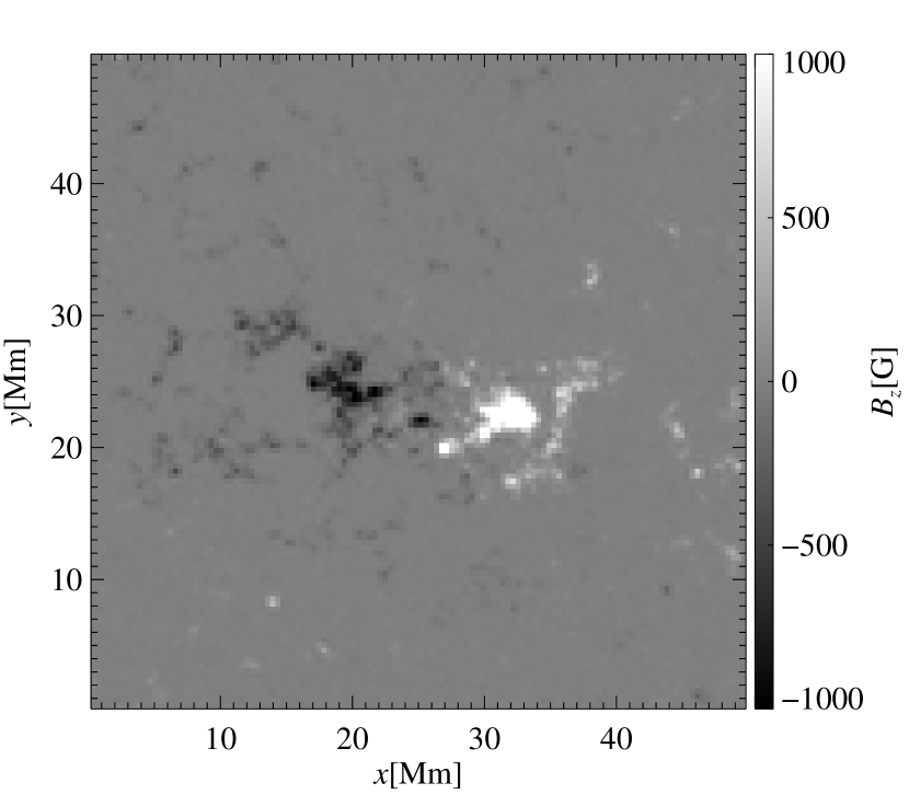
Figure 1: Initial vertical magnetic field at the bottom boundary of the simulation. This is based on a magnetogram from active region AR 11102 observed with HMI. See Sect. 3.2.

In the horizontal $x$-$y$ plane, all variables are periodic. At the bottom boundary, the temperature $T$ and density $\rho$ have fixed values whereas the horizontal velocities, $u_{x}$, $u_{y}$ have zero vertical gradients. The vertical velocity $u_{z}$ is set to satisfy the divergence-free condition $\bm{\nabla}\cdot\bm{u}=0$. We also prescribe a photospheric velocity driver which generates random photospheric motions; these are time-dependent and create a velocity distribution and spectrum similar to the one observed on the solar photosphere. As a result, we shuffle the footpoints of the magnetic loops mimicking the solar photospheric flows in a similar way to, e.g., Gudiksen & Nordlund (2002, 2005b, 2005a). At the top boundary, all velocity components are zero. To prevent any heat flux going in or out of the computational domain, the gradients of temperature and density are set to zero. The magnetic field is potential both for the bottom and the top boundary.

4 Numerical experiments

4.1 Setup

Table 1: Summary of numerical experiments.

Run	a	$\Phi$ [Mx]
1B	1	$7.4\times 10^{20}$
2B	2	$1.5\times 10^{21}$
5B	5	$3.7\times 10^{21}$
10B	10	$7.4\times 10^{21}$
20B	20	$1.5\times 10^{22}$

The main idea of this work is to start with an active region hosting only a small amount of total (unsigned) magnetic flux and then run models with increasing magnetic flux. Our aim is to study how the increase of the photospheric magnetic field strength contributes to the heating, and thus the X-ray emission of the solar or stellar corona.

Here we report the results from a set of five numerical experiments. The original total unsigned surface magnetic flux of AR11102 is around $7\times 10^{20}$ Mx, which is a typical value of a small solar active region. We increase the flux by multiplying the $B_{z}$ component of the surface magnetic field by a constant ranging from 1 to 20 (see Table 1). The spatial structure of the magnetic field remains unchanged. In all cases, the total magnetic flux at the bottom boundary is zero, that is, the surface magnetogram is balanced.

The heating of the coronal loops originates from the dissipation of Poynting flux into heat. More specifically, the conversion of the photospheric magnetic energy to thermal energy is due to the dissipation of the currents created by the random photospheric motions. The stronger the magnetic field, the more Poynting flux reaches the corona, resulting in a higher temperature and X-ray emission.

In our setup, the different total unsigned magnetic fluxes correspond to peak values of the magnetic field ranging from 1 to 20 kG inside the spots; hence our naming convention in Table 1. The value of 20 kG is very high for a solar active region. Recent observations of solar active regions measured maximum values of the magnetic field strength on the order of 8 kG (Castellanos Durán et al. 2020). However, this high value was observed in only very small area on the active region light bridge. Typically the peak magnetic field strengths on solar active regions are on the order of 2 kG to 3 kG. Therefore, of the numerical experiments listed in Table 1, the 5B run can be considered to represent a typical solar active region, with a typical value for the total unsigned flux. However, higher values of surface magnetic field could be a common feature of very active stars (Reiners et al. 2014), and so the runs 10B and 20B could be considered to be representative of more active stars.

The increase in the surface magnetic field is not the only way to increase the surface magnetic flux. Alternatively, we could increase the horizontal extent of an active region while keeping the peak magnetic field strength the same. This will be the main focus of a future study.

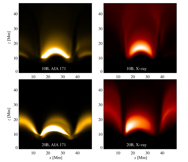
Figure 2: Side view of the computational domain showing coronal emission. The left two panels show the emission as it would be seen by the 171 Å channel of AIA starting from around 1 MK. The two right-hand panels show X-ray emission as seen by XRT sampling higher temperatures. Here we show snapshots of the two more active models, runs 10B and 20B. The emission here is integrated along the $y$ direction which corresponds to an observation near the limb (of the Sun or a star). The snapshot is taken at $t$=230 min; i.e., in the relaxed state. See Sect. 4.2.

4.2 Synthesized emission: X-rays and EUV

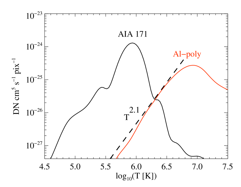
Figure 3: Temperature response function for the AIA instrument on board SDO and the XRT on board Hinode. The black line shows the 171 Å channel of the AIA, the red line shows the Al-poly filter of the XRT. For illustration purposes, the black dashed line indicates a power-law approximation to XRT at temperatures below $10^{7}$ K. See Sect. 4.2.

Coronal loops are mostly observed in extreme ultraviolet (EUV) wavelengths and X-rays because these wavelengths give access to the 1 MK plasma in the corona, and in these wavelengths, the dilute corona is also visible in front of the solar (or stellar) disk, which is very bright in the visible range. Therefore, we synthesize the emission in one EUV and one X-ray band. For the EUV band we choose the widely used 171 Å band as seen by the Atmospheric Imaging Assembly (AIA; Lemen et al. 2012) on board the Solar Dynamic Observatory (SDO; Pesnell et al. 2012). Throughout the present paper we only consider the 171 Å channel of the EUV spectra and not the whole EUV range. We use the 171 Å channel of AIA as a reference for plasma at 1 MK and how it compares with plasma at higher temperature emitting in X-rays. For the X-ray emission, we use the Al-poly filter of the solar X-ray telescope (XRT; Golub et al. 2007) on board the Hinode observatory (Kosugi et al. 2007).

As mentioned in Sect. 2, the optically thin radiative losses through lines and continua in the corona observed in a given wavelength band are given through

$$\varepsilon=n_{\rm{e}}^{2}\,R(T),$$ (15)

where $n_{\rm{e}}$ is the electron density and $R(T)$ the temperature response (or contribution) function. The response needs to be calculated for each instrument (or filter) using the effective area depending on wavelength and the spectral lines forming in the wavelength region covered by the instruments. To calculate $R(T)$ for the 171 Å channel of AIA and the Al-poly filter of XRT, we use the routines in the Chianti data base v9 Dere et al. (1997, 2019) as they are available in the SolarSoft package. The response functions $R(T)$ for AIA 171 Å and XRT Al-poly are shown in Fig. 3. To calculate the synthetic images as they would be observed by AIA or XRT, $\varepsilon$ from Eq. (15) has to be integrated through the computational domain along the chosen line of sight. The samples for both channels for the 10B and 20B runs are shown in Fig. 2. These are integrated along the $y$ direction which would correspond to an observation near the limb.

4.3 Horizontal averages

The increase of the surface magnetic field results in an increase in temperature and density in the coronal part of the domain. We calculate the horizontal averages of temperature $T$, density $\rho$, and the vertical component of the Poynting flux $S_{z}$ and then average these in time for an interval of 1 hour. During this time interval the computation reached a relaxed state, that is, the respective (spatially averaged) quantities show only rather small changes around a mean value (see Sect. 4.4 and Fig. 5). The average vertical stratification of $T$, $\rho$, and $S_{z}$ is shown in Fig. 4.

4.3.1 Average Poynting flux deposited in the corona

The photospheric horizontal motions lead to an upward-directed flux of magnetic energy, the Poynting flux. Here we concentrate on its vertical component,

$$S_{z}=\eta(\bm{j}\times\bm{B})\big{|}_{z}-\frac{1}{\mu_{0}}(\bm{u}\times\bm{B}\times\bm{B})\big{|}_{z},$$ (16)

which is shown in Fig. 4c for the different runs. In the main part of the computational domain, the $\bm{u}{\times}\bm{B}{\times}\bm{B}$ term dominates and (on average) is positive, that is, upwards directed. The first term including the current, $\bm{j}$, is significant only near the bottom where boundary effects of the driving cause high currents. Energetically, this is not relevant, because there the density is high enough that the heating through the currents has virtually no effect.

As we increase the total unsigned magnetic flux from one experiment to the next, the energy stored in the corona increases. The magnetic energy in excess of that of a potential field will be (partly) dissipated and converted into heat. The higher amount of dissipated (free) magnetic energy in the runs with higher magnetic flux leads to higher coronal temperatures and density (see Fig. 4a and Fig. 4b). This is just as expected from the RTV scaling laws (Eqs. 1 and 2) as we discuss later in Sect. 6.2 (see also Fig. 8).

The Poynting flux for the runs 1B and 2B (i.e., black and blue solid lines in Fig. 4c) coincide in the lower part of the atmosphere (below 6 Mm). We find this to be the case only for the specific time frame used for the time averaging (i.e., from 3.5 to 4.5 hrs). For the time period before 3.5 hrs the Poynting fluxes for the runs 1B and 2B differ by a factor of two, as expected. This peculiar behavior is only observed for the run 1B for which the magnetic field is too low to even produce a proper corona. We observe this particular behavior only at the lower atmosphere while for the coronal part shown in Fig. 5, we see a clear distinction between runs 1B and 2B. However, as we only consider values on the coronal part for our results, this peculiar behavior will not have any effect on the results presented in the following section.

Furthermore, the Poynting flux of the 1B run at the base of the corona (i.e. at an average temperature of around 0.1 MK) barely reaches 50 W/m². Typical estimations based on observations suggest an energy requirement of around 100 W/$\rm{m}^{2}$ for the quiet Sun and 10⁴ W/$\rm{m}^{2}$ above active regions (Withbroe & Noyes 1977). Therefore, we cannot expect this run with the lowest magnetic activity to produce a megakelvin corona.

4.3.2 Average temperature and density

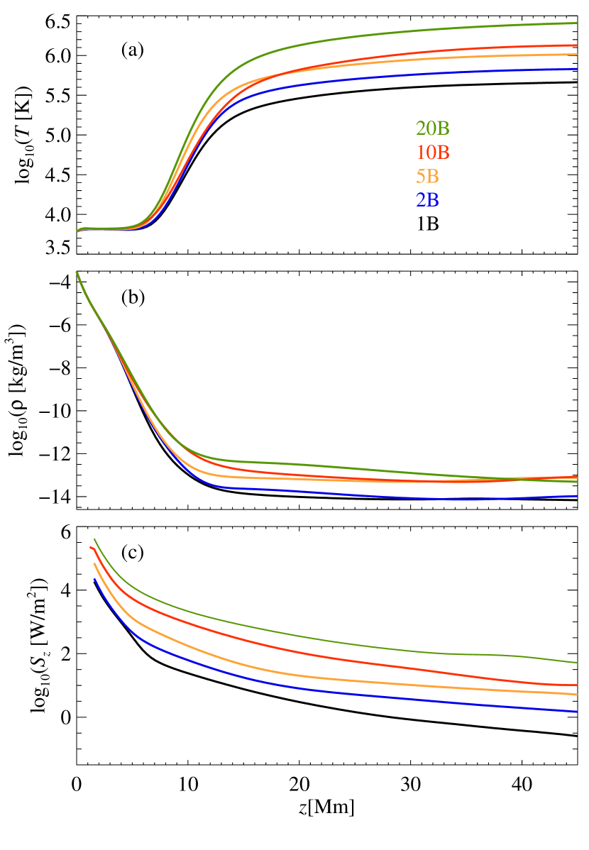
Figure 4: Horizontal averaged quantities as a function of height. We show temperature $T$ (panel a), density $\rho$ (panel b), and the vertical component of the Poynting flux $S_{z}$ (panel c). The colors represent the different runs as indicated in the legend (cf. Table 1). The quantities are averaged horizontally for each snapshot and then in time for 1 hour (between the time-point at 3.5 hr and that at 4.5 hr, as indicated in Fig. 5 by the vertical dashed lines. For the Poynting flux we omitted the first three grid points that show boundary effects. See Sect. 4.3.

All of our simulations self-consistently form a hot upper atmosphere, where the temperature is about two orders of magnitude higher than at the surface (cf. Fig. 4a). A higher total unsigned flux in the photosphere (cased 1B through 20B) corresponds not only to higher Poynting fluxes, but also to higher temperatures and density. The values shown in Fig. 4a and b are averages only, so the peak values are significantly higher, up to 5 MK and more.

The experiment with the lowest magnetic activity (run 1B) fails to create a megakelvin hot corona, as expected. Still, we consider it in the analysis of the power-law relation in Sect. 5. The main focus of this work is to relate the coronal emission to the surface magnetic activity through a number of numerical experiments, and in this sense a model that is not active enough to produce a megakelvin corona also provides valuable insight.

Besides the increased temperature and density, the models with higher magnetic activity also have the transition region located at lower heights. From this, it is clear that the height where the average temperature reaches 0.1 MK is lower for the runs with more magnetic flux. The higher energy input leads to a higher heat flux back to the Sun. Because the radiation is most efficient at lower temperatures (at 0.1 MK and below), in equilibrium the transition region will be found at lower temperatures and thus higher densities where it can radiate the energy. Consequently, the density (and the pressure) throughout the corona will be higher, as is indeed seen in our simulations.

The average density profile $\rho$ displays similar (qualitative) behavior to the temperature. In the coronal part, the density is high for the runs with higher magnetic flux (Fig. 4b). Following a steep drop over many orders of magnitude in the low atmosphere, the density remains almost constant in the coronal part. This is simply because of the large barometric (pressure) scale height at high temperatures. At 1 MK, this scale height is about 50 Mm and thus comparable to the vertical extent of our computational domain; hence the horizontally averaged pressure and density are roughly constant in the coronal part of our box.

4.4 Temporal evolution

The quantities we consider in our model vary significantly with time, especially during the early phase of the simulations. To investigate the average behavior of our model, we have to consider a time-frame of the numerical model where the system reaches a relaxed (or evolved) state. During that state, the quantities show (comparably small) variations around an average value.

To illustrate this, we first consider the total heating in the coronal part of the computational domain. We define the coronal part as the volume above the height where the horizontally averaged temperature is $10^{5}$ K. Because the temperature gradient in the transition region around $10^{5}$ K is rather steep, the exact choice of this temperature is inconsequential. We therefore define the total coronal heating $H_{\rm{tot}}$ as the volume integral over this coronal part, here symbolized by the subscript ’cor’,

$${H_{\rm{tot}}}=\int_{\rm{cor}}\eta\mu_{0}\bm{j}^{2}dV.$$ (17)

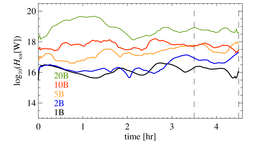
Figure 5: Total coronal heating $H_{\rm{tot}}$ as a function of time. The vertical dashed lines indicate the time span used for the temporal averages. The colors represent the different runs as indicated in the legend (cf. Table 1). See Sect. 4.4.

The temporal variation of the heating is shown in Fig. 5 for the five models with different magnetic activity. We see a clear ordering of the heating with the surface magnetic flux (increasing for run 1B through 20B), which we discuss in more detail in Fig. 7 and Sect. 6.1. In terms of the temporal evolution, we find that the heat input reaches a relaxed state rather quickly, probably within less than an hour. This is expected, because the stresses applied on the magnetic field in the photosphere will propagate with the Alfvén speed. The corresponding Alfvén crossing time for perturbations to cross the whole box is on the order of minutes.

The situation for the relaxation time is different when considering the coronal emission in X-rays and the 171 Å channel of AIA. Here it turns out that we have to wait for about three hours before the models reach a relaxed state. Mainly, this is because of the radiative cooling time under typical coronal conditions which is on the order of 1 hour (Aschwanden 2005). Therefore, we examine the temporal evolution of the coronal radiation in some more detail below.

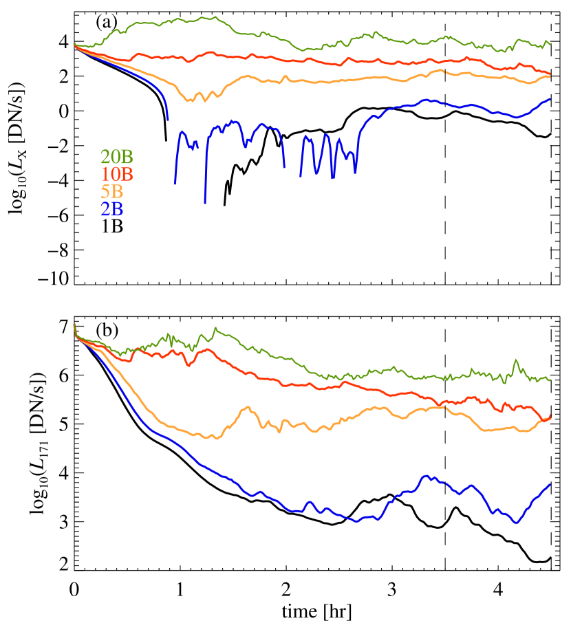
Figure 6: Temporal evolution of the coronal emission from integration over the whole computational domain. Panel (a) shows the X-ray emission as seen by XRT in the Al-poly filter, panel (b) the EUV emission as it would be seen by AIA in the 171 Å channel. The vertical dashed lines indicate the time-span used for time averaging. The colors represent the different runs as indicated in the legend (cf. Table 1). See Sect. 4.4.

We now turn to the variability of the X-ray and EUV emission represented by the 171 Å channel of AIA (see Fig. 6). Because the lower cool part of the atmosphere does not produce any significant amount of X-rays or EUV, we simply integrate the coronal emission over the whole computational domain. This is equivalent to the luminosity originating from the domain, $L_{\rm{X}}$ and $L_{\rm{171}}$. Because we use the temperature response functions for XRT and AIA (Sect. 4.2, Fig. 3), we get the counts per second as expected for the respective instrument from the whole loop in the box (cf. Fig. 2). For the comparison between the different model runs, it is important that we use the same scale for the different models. Based on this, we see a clear scaling of the coronal emission with magnetic activity, in a similar way to what we see for the heat input. We discuss this in more detail in Fig. 9 and Sect. 6.3.

Overall, the coronal emission shows an initial drop on the timescale of almost an hour, in particular for EUV channel of AIA 171 Å in the runs with low magnetic activity. This is because the atmosphere of the initial condition is rather hot, and the plasma is cooling down until it reaches a new equilibrium after a few coronal radiative cooling times (Fig. 6). Here we see that all model runs reach a relaxed state after about 2.5 to 3 hours.

The relative variability for the 1B and 2B runs is larger than for the runs with higher magnetic activity. Still, the absolute variability seen in the more active runs is much higher (the logarithmic plot in Fig. 6b shows the relative variation). Also, when following run 1B further in time, the emission in the 171 Å channel is not dropping further. The situation is different when considering other channels like the X-ray regime which considers hotter plasma. There, the variability is relatively low even for the low magnetic activity runs.

Thus, with some safety margin we can assume that from 3.5 to 4.5 hours the models have reached a relaxed state (see vertical dashed lines in Figs. 5 and 6). All the time averages discussed in our study are taken over this time frame.

5 Scaling relations in numerical experiments

To characterize the model runs with different magnetic activity, that is, unsigned magnetic surface flux, we investigate the scaling relations in the form of power laws between different parameters. In Sect. 4 we show that the enhancement of the photospheric magnetic flux leads to a substantial increase in temperature, density, Poynting flux, and coronal emission. In this section, we discuss the power-law relations of various quantities averaged in space and time quantities. We discuss these results in Sect. 6 including the study of Zhuleku et al. (2020).

We first concentrate on the relation between the vertical component of the average Poynting flux ${\langle}S_{z}{\rangle}$ and both the unsigned surface magnetic flux $\Phi$ and the averaged total coronal heating ${\langle}H_{\rm{tot}}{\rangle}$ (see Fig. 7). Each cross in the two figures represents the average value of the respective quantities in each individual numerical model (cf. Table 1). Here we take the horizontal average of the Poynting flux ${\langle}S_{z}{\rangle}$ at the height where the horizontally averaged temperature is $10^{5}$ K, that is, the base of the corona and average it in time from 3.5 to 4.5 hr (see Sect. 4.4). This represents the energy flux (per unit area) into the corona. The total averaged coronal volumetric heating ${\langle}H_{\rm{tot}}{\rangle}$ is calculated according to Eq. (17) and then averaged between times 3.5 and 4.5 hr as discussed in Sect. 4.4. The unsigned surface flux $\Phi$ is the integral over the bottom boundary, that is, the stellar surface which is constant in time. The bars in Fig. 7 indicate the standard deviation of the respective quantity in time. For relations displayed in Fig. 7 we perform power-law fits (indicated by the red line) that result in

$${\langle}S_{z}{\rangle}\propto\Phi^{\beta}\leavevmode\nobreak\ \leavevmode\nobreak\ \leavevmode\nobreak\ \leavevmode\nobreak\ \leavevmode\nobreak\ \leavevmode\nobreak\ \leavevmode\nobreak\ \beta\leavevmode\nobreak\ =1.71\pm 0.42,$$ with (18)

$${\langle}S_{z}{\rangle}\propto{\langle}H_{\rm{tot}}{\rangle}^{\Gamma} \Gamma=0.88\pm 0.22.$$ with (19)

Here $\Gamma$ corresponds to $1/\gamma$ from the analytical model in Eq. (6) and Zhuleku et al. (2020). The two scalings (18) and (19) imply that the heating increases roughly quadratically with magnetic flux, ${\langle}H_{\rm{tot}}{\rangle}\propto\Phi^{1.94}$.

As a next step, we relate the coronal temperature $T$ and density $\rho$ to the total coronal heating ${\langle}H_{\rm{tot}}{\rangle}$. Here we test to what extent the coronal temperature and density in our numerical model deviate from the analytic RTV scaling laws as given in Eqs. (1) and (2). To this end, we calculate the average temperature ${\langle}T{\rangle}$ and density ${\langle}\rho{\rangle}$ in the corona in a height range from $z{=}10$ Mm to 20 Mm for each of the models. We choose this particular height range because this is where the bright structures appear (see Fig. 2). If we were to also include higher regions of the box, the averages would no longer represent the visible parts of the corona. In addition, we average ${\langle}T{\rangle}$ and ${\langle}\rho{\rangle}$ in time from 3.5 to 4.5 hr as discussed in Sect. 4.4. We show the corresponding plots including the power-law fits of ${\langle}T{\rangle}$ and ${\langle}\rho{\rangle}$ as a function of the total coronal heating $H_{\rm tot}$ in Fig. 8. The power-law fits yield

$${\langle}T{\rangle}\leavevmode\nobreak\ \propto\leavevmode\nobreak\ {\langle}H_{\rm{tot}}{\rangle}^{a} a=0.24\pm 0.03,$$ with (20)

$${\langle}\rho{\rangle}\leavevmode\nobreak\ \propto\leavevmode\nobreak\ {\langle}H_{\rm{tot}}{\rangle}^{b} b=0.76\pm 0.05.$$ with (21)

Finally, we address the relation of the X-ray emission to the heating rate and the unsigned surface magnetic flux. As the photospheric magnetic flux is larger for models with higher magnetic activity, the total dissipated energy is also larger. Because the X-ray emission is expected to increase with the heating rate, it should also be larger for higher unsigned magnetic flux. For the analysis, we consider the averaged emission, ${\langle}L_{\rm{X}}{\rangle}$, that is integrated over the whole computational domain and averaged in the same way as the other quantities from 3.5 to 4.5 hr. The corresponding relations are plotted in Fig. 9 and Fig. 10a, and the power-law fits give

$${\langle}L_{\rm{X}}{\rangle}\leavevmode\nobreak\ \propto\leavevmode\nobreak\ \Phi^{m}\,\leavevmode\nobreak\ \leavevmode\nobreak\ \leavevmode\nobreak\ \leavevmode\nobreak\ \leavevmode\nobreak\ m=3.44\pm 0.28,$$ with (22)

$${\langle}L_{\rm{X}}{\rangle}\leavevmode\nobreak\ \propto\leavevmode\nobreak\ {\langle}H_{\rm{tot}}{\rangle}^{q} \>q=1.78\pm 0.15.$$ with (23)

We apply the same integration and time averaging to the EUV emission as seen by AIA in its 171 Å channel. Its relation to the heat input is displayed in Fig. 10b and the power-law fit reveals an almost linear relation,

$${\langle}L_{\rm{171}}{\rangle}\leavevmode\nobreak\ \propto\leavevmode\nobreak\ {\langle}H_{\rm{tot}}{\rangle}^{p}\qquad\mbox{with}\qquad p=1.05\pm 0.09.$$ (24)

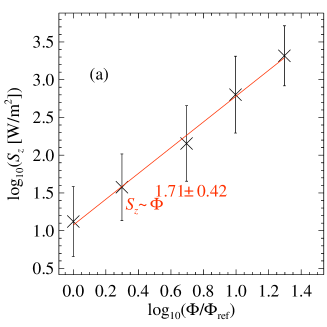
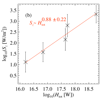
Figure 7: Scaling of average Poynting flux ${\langle}S_{z}{\rangle}$ with unsigned surface flux $\Phi$ and average coronal heating ${\langle}H_{\rm tot}{\rangle}$. Each data point represents an average for one of the model runs with different unsigned surface magnetic flux as listed in Table 1. As a reference for the magnetic flux, $\Phi_{\rm{ref}}$, we choose the magnetic flux of the least active setup, run 1B (cf. Table 1). The bars represent the standard deviation of $S_{z}$ in time. The red lines are power-law fits to the data. See Sects. 5 and 6.1.

6 Discussion

6.1 Energy input into the corona

The solar coronal heating problem and the underlying physical mechanism has been extensively discussed over the last 70 years. Two of the main mechanisms that are being considered are the Alfvén-wave model (e.g., van Ballegooijen et al. 2011) and the field-line braiding or nanoflare model (Parker 1972, 1983). In these two processes, the Poynting flux, and hence the heat input, have a different dependence on the magnetic field. A simple estimate for these dependencies was given by Fisher et al. (1998), and here we follow their arguments. For an Alfvén wave with constant amplitude, the Poynting flux will be proportional to the propagation speed, that is, the Alfvén velocity, and hence to the magnetic field $B$, $S_{z}\propto B$. For the field-line braiding, the Poynting flux will be set by the driving motions with speed $u$ and the magnetic field, $S\propto u{\times}B{\times}B$, and hence the scaling will be $S_{z}\propto B^{2}$ (assuming that the driving motions do not change with $B$).

In our numerical experiments we find a power-law scaling between Poynting flux and (unsigned) magnetic flux with a power-law index of about $1.7{\pm}0.4$; see Eq. (18) and Fig. 7a. Within the uncertainties this is consistent with the above (analytical) estimate of 2. This is not surprising, because our in our model we drive the coronal magnetic field through footpoint motions consistent with the field-line braiding scenario. Still, it is reassuring to recover this scaling by our numerical model.

Observationally, it is clear that Alfvén waves are present in the corona (e.g., Tomczyk et al. 2007). Still, it remains unclear as to whether or not the energy they carry is sufficient to energize the corona. Waves might play a role in the quiet Sun corona, but they appear to be unable to heat active regions McIntosh et al. (2011). Our particular model can contribute little to this discussion, because we do not fully resolve Alfvén waves, which is because of the comparably large dissipation.

Finally, we expect that the total energy dissipated in the coronal volume matches the Poynting flux at the base of the corona. In this case, the Poynting flux should scale linearly with the total amount of energy dissipated in the corona. In our numerical experiments, we find a power-law relation with a power-law index of about $0.9{\pm}0.2$, which is consistent with linear; see Eq. (19) and Fig. 7b.

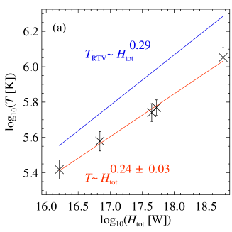
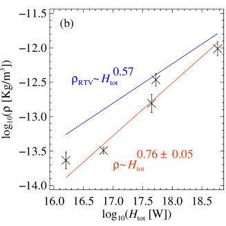
Figure 8: Scaling of average temperature ${\langle}T{\rangle}$ and density ${\langle}\rho{\rangle}$ with average coronal heat input ${\langle}H_{\rm{tot}}{\rangle}$. Each data point represents an average for one of the model runs with different unsigned surface magnetic flux listed in Table 1. The bars represent the standard deviation of the spatial averages of $T$ and $\rho$ in time. The red lines are power-law fits to the data. The blue lines indicate what is expected from the RTV scaling laws. See Sects. 5 and 6.2.

6.2 RTV scaling laws compared to numerical experiments

One obvious check for the numerical experiments is to what extent the average quantities will follow the RTV scaling laws of Eqs. (1) and (2). Because of the spatial and temporal variability we cannot expect a perfect match, but the average quantities should roughly follow these scalings, as was found in an earlier model for one single (small) solar active region (Bourdin et al. 2016).

The original RTV scalings in Eqs. (1) and (2) include a dependence on the loop length $L$. However, in our numerical models the physical size of the computational box is kept constant. Therefore, the coronal loops can be considered to have similar lengths. Consequently, in this study we only have to consider the dependence of temperature and density on (total) heating in the coronal volume, $H_{\rm{tot}}$.

For a comparison to the RTV scalings one should not only compare the power-law indices of the scaling, but also the absolute values of the temperature $T$ and density $\rho$ as given in the original paper by Rosner et al. (1978). To calculate the predictions from the RTV scalings, that is, $T_{\rm{RTV}}$ and $\rho_{\rm{RTV}}$, we use a loop length of $L{=}30$ Mm, which is similar to the average loop length we find in the emission patterns synthesized from the model (see Fig. 2). For the volumetric heating rate we use the (total) heating in the coronal volume, ${\langle}H_{\rm{tot}}{\rangle}$, divided by the coronal volume, which gives the (average) volumetric heating. The resulting variation of $T_{\rm{RTV}}$ and $\rho_{\rm{RTV}}$ with ${\langle}H_{\rm{tot}}{\rangle}$ is shown in Fig. 8 (blue lines). The power law indices of 0.29 and 0.57 for these correspond to 2/7 and 4/7 in Eqs. (1) and (2).

The power-law relation of the average temperatures ${\langle}T{\rangle}$ and density ${\langle}\rho{\rangle}$ in the numerical models with ${\langle}H_{\rm{tot}}{\rangle}$ are close to what is expected from RTV. However, both the temperature and the density are significantly lower, by about a factor two and three; see Fig. 8 and Eqs. (20) and (21).

The reason for this underestimation is mainly due to the averaging process of the temperature and density. The bright loops are hotter and denser than the ambient corona, meaning that the averages underestimate the values corresponding to the RTV scaling relations. Still, we conclude that the numerical models and the analytical scaling relations are consistent (as an order-of-magnitude estimation).

6.3 Relation of X-ray emission to surface magnetic flux

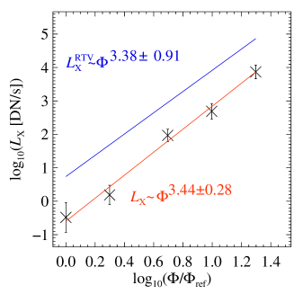
Figure 9: Scaling of average X-ray emission ${\langle}L_{\rm{X}}{\rangle}$ with unsigned surface flux $\Phi$. Each data point represents an average for one of the model runs with different unsigned surface magnetic flux listed in Table 1. As a reference for the magnetic flux, $\Phi_{\rm{ref}}$, we choose the magnetic flux of the least active setup, run 1B (cf. Table 1). The bars represent the standard deviation of $L_{\rm{X}}$ in time. The red lines are power-law fits to the data. The blue lines show the analytic power-law relations based on the RTV scaling laws; see Sects. 5, 6.3 and 6.4.

The central result of our study is the power-law relation between the synthetic X-ray emission $L_{\rm{X}}$ and the unsigned surface magnetic flux $\Phi$. We show this relation $L_{\rm{X}}\propto\Phi^{m}$ with a power-law index $m$ of about $3.4{\pm}0.3$ in Fig. 9; see also Eq. (22).

This $L_{\rm{X}}$ versus  $\Phi^{m}$ relationship has been extensively discussed in numerous observational studies of the Sun and of stars of different spectral types (see e.g., Fisher et al. 1998; Pevtsov et al. 2003; Vidotto et al. 2014). However, the physical reasons behind the observed power-law relation remain unclear. Observations of various solar features and solar-like stars suggest a relation close to but slightly steeper than linear, i.e., $m{\gtrsim}1$ (e.g., Fisher et al. 1998; Pevtsov et al. 2003).

We can estimate this power-law index $m$ from observations by comparing the (average) X-ray emission and magnetic field of the Sun to those of other stars. The Sun has an average magnetic field of roughly 10 G (Cranmer 2017), active stars show average fields of about 1 kG (Saar 1996; Saar & Brandenburg 2001). This reveals a difference of a factor of 100 in magnetic field strength. At the same time the X-ray emission increases from the Sun to active stars by a factor of 1000 (X-ray-rotation activity relation) (see e.g., Pizzolato et al. 2003). From this one can conclude that the $L_{\rm{X}}$ versus $\Phi$ increases as a power law with an of index $m=1.5$. However, more recent studies find the power law to be close to quadratic ($m{=}1.8$; Vidotto et al. 2014) or even steeper ($m{=}2.68$; Kochukhov et al. 2020). While Kochukhov et al. (2020) considered stars similar to the Sun in terms of spectral type, all these were considerably more active than the Sun in terms of X-ray luminosity. The large sample of Vidotto et al. (2014) also mostly contained stars significantly more active than the Sun.

An almost linear relation of $L_{\rm{X}}$ versus  $\Phi$ could be simply understood by increasing the number of active regions on a (solar-like) star. If the filling factor of active regions is low and one simply doubles the number of active regions, both the total unsigned magnetic flux on the stellar surface and the X-ray emission would double; hence, the linear relation between $L_{\rm{X}}$ and $\Phi$. This, in principle, could explain the findings of Fisher et al. (1998) and Pevtsov et al. (2003).

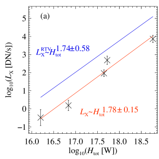
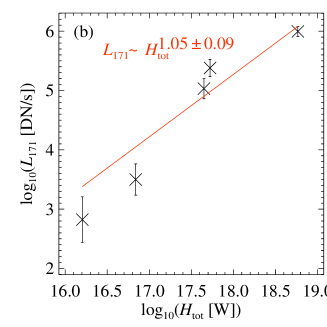
Figure 10: Scaling of average X-ray and 171 Å emission as observed by AIA, ${\langle}L_{\rm{X}}{\rangle}$, and ${\langle}L_{\rm{171}}{\rangle}$ with average coronal heating ${\langle}H_{\rm tot}{\rangle}$ for model runs listed in Table 1. The bars represent the standard deviation of $L_{\rm{X}}$ and $L_{\rm{171}}$ in time. The red lines are power-law fits to the data. The blue line in panel (a) indicates what is expected from the RTV scaling laws. See Sects. 5 and 6.5.

Active stars show X-ray luminosities (compared to their bolometric luminosity) that can be three or more orders of magnitude larger than that of the Sun(e.g., Vidotto et al. 2014). In this case there would simply not be enough space on the star to cover it with enough (solar-like) active regions. This means that the X-ray emission per active region has to increase. This is exactly what we find in our model when increasing the magnetic flux of an active region while keeping its size (i.e. area) the same. This leads to a steep increase in X-ray luminosity with surface magnetic flux, an increase that is even steeper than observed: the power-law index $m$ for $L_{\rm{X}}\propto\Phi^{m}$ is about 3.4 in our model, while the largest value found in observations is below 2.7 Kochukhov et al. (2020). This overestimation of the power-law index by our model indicates that on real stars we might find a mixture of an increase in the numbers of active regions together with an increase in the peak magnetic field strength (or magnetic flux per active region) for more active stars.

Furthermore, the power-law index $m$ might be overestimated by our model. Strong surface magnetic fields could quench the horizontal motions and consequently reduce the resulting Poynting flux (e.g., Gudiksen & Nordlund 2005b). This is not included in our model. In Appendix A, we discuss the impact that this quenching could have on our estimations of the power-law relations. We find that a realistic quenching of the horizontal velocities by about a factor of three would reduce the index $m$ of the power-law relation between X-ray emission and magnetic field, $L_{\rm{X}}\propto\Phi^{m}$ by about 25% to around 2.6. This would bring the value for $m$ derived from our model closer to the index derived by recent observations.

6.4 Analytical model for scaling of X-ray emission

We now compare the scaling of $L_{\rm{X}}\propto\Phi^{m}$ to some basic analytical considerations. In an earlier study we derived an analytical scaling of the X-ray emission with surface magnetic flux that is based on the RTV scaling relations Zhuleku et al. (2020). As discussed in the summary of that model in Sect. 2, there we used a scaling of active region size with (unsigned) magnetic flux based on solar observations, see Eq. (7). In contrast, in our numerical model we keep the size or area covered by the active region constant; hence, here the power-law index in Eq. (7) is $\delta{=}0$. This simplifies our analytical scaling from Eq. (3) to

$$m=\frac{\beta\gamma}{7}(2\alpha+8).$$ (25)

According to Eq. (4), $\alpha$ is the power-law index relating the temperature response (or contribution) function to temperature. Here we approximate this for X-rays as seen by the XRT on Hinode (see Fig. 3), where a power-law fit yields

$$R_{\rm{X}}\propto T^{\alpha}\quad\mbox{with}\quad\alpha=2.1\pm 0.2.$$ (26)

We provide a more extensive discussion on the temperature responses for different instruments in Zhuleku et al. (2020).

We take the other two parameters $\beta$ and $\gamma$ in Eq. (25) from the relations of the Poynting flux to the unsigned surface magnetic flux and the total heating in Eqs. (18) and (19), with $\gamma{=}1/\Gamma$ in Eq. (19). This results in the analytic scaling (based on RTV) of

$$L_{\rm{X}}^{\rm{RTV}}\propto\Phi^{m^{\prime}}\quad\mbox{with}\quad m^{\prime}=3.38\pm 0.91.$$ (27)

This is overplotted on the results from the numerical experiments in Fig. 9 as a blue line. We conclude that this power-law index is in good agreement with the value we obtained from the numerical models, see Eq. (22) and Fig. 9.

Just as for the comparison to the RTV scalings in Sect. 6.2, also here it is not sufficient to find a match of the power-law index; the absolute values of the derived X-ray emission also have to be of the same order for a good match. To get the constant of proportionality in Eq. (27), we have to assign a volume of the emitting structure described in the analytical scaling. For the comparison to our numerical model we therefore assign the volume of the loop(s) dominating the coronal emission. Using the loops in Fig. 2 as a guideline, these have a length and a radius of about $L{\approx}30$ Mm and $r{\approx}2.5$ Mm. With the volume of $V=\pi R^{2}L$ we then find the total X-ray radiation from the loops based on the (RTV) scaling relations of $L_{\rm{X}}^{\rm{RTV}}$. Within an order of magnitude these match what we find in the numerical study. The deviation is mainly because of the factor of about three difference in density (cf Sect. 6.2) which enters the emission quadratically.

6.5 X-ray and EUV emission versus coronal energy input

Our current understanding of solar physics would lead us to believe that a higher energy input into the corona should result in a higher X-ray emission. Indeed, this is what we find in Fig. 10a. However, we find an almost quadratic relationship, ${\langle}L_{\rm{X}}{\rangle}\propto{\langle}H_{\rm tot}{\rangle}^{1.8}$, cf. Eq. (24). This nonlinearity is counter-intuitive: Assuming that the plasma in our numerical model has reached a relaxed state, then whatever energy reaches the corona should be radiated away as X-ray emission (i.e., naively, we would expect a linear dependence).

This (roughly) quadratic relation can be understood when going back to the RTV scalings. The X-ray emission is given by $L_{\rm{X}}\propto n^{2}\,R_{\rm{X}}$. Combining this with the fit to the X-ray response function in Eq. (26) and the RTV scaling relations in Eqs. (1) and (2) provides the analytical scaling for the X-ray emission with (average) coronal heat input,

$$L_{\rm{X}}^{\rm{RTV}}\propto{\langle}H_{\rm{tot}}{\rangle}^{q^{\prime}}\quad\mbox{with}\quad q^{\prime}=1.74\pm 0.58.$$ (28)

This is shown in comparison to the results from the numerical model in Fig. 10a as a blue line. As before, we assume a constant loop length, because the active region size is the same for all numerical experiments.

This consideration provides an understanding of the nonlinear relation between X-ray output and heat input. In the corona the energy input will be only partly balanced by the X-ray output (heat conduction, wind outflow, and radiation at other wavelengths also play their respective roles). Because the X-ray output shows a nonlinear temperature dependence, naturally it will also be connected in a nonlinear fashion to the heat input. The simple RTV scaling relations, together with the temperature response of X-ray emission give rise to the roughly quadratic dependence of X-rays on heat input.

The situation changes when investigating another wavelength region, which essentially implies probing a different temperature range. For this we use the channel as seen by AIA at 171 Å. The emission from the 171 Å channel of AIA in this band mostly originates from temperatures around 1 MK (cf. Fig. 3). If we apply the same analysis as for the X-ray emission, the numerical experiments show an almost linear scaling with heat input, ${\langle}L_{\rm{171}}{\rangle}\propto{\langle}H_{\rm tot}{\rangle}^{1.1}$; see Fig. 10b. The reason this relation is less steep than for the X-rays is because of the different temperature response in the EUV.

The response of the 171 Å channel of AIA cannot be simply approximated by a power law (see Fig. 3). However, over the temperature range of most our models, as a very rough zeroth-order approximation we could assume the response in the 171 Å channel to be constant. This would be consistent with the power-law index for the response function, that is,  $\alpha$ in Eq. (4), being equal to zero. Following the above procedure for the X-rays, in analogy to Eq. (28) we would find $L_{\rm{171}}^{\rm{RTV}}\propto{\langle}H_{\rm{tot}}{\rangle}^{1.14}$ for the 171 Å channel emission. This result compares well with the numerical experiments (cf. Fig. 10b), but certainly it has to be taken cum grano salis, because of our very rough assumption of $\alpha{=}0$. This is why we do not overplot an analytical approximation in Fig. 10b as we did for the other scaling relations. Still, this consideration underlines the importance of the temperature response in establishing a relationship between coronal emission and heat input.

6.6 Relating X-rays to EUV emission

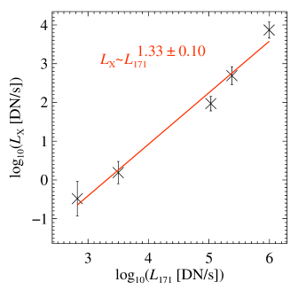
Figure 11: Scaling of averages of X-ray emission ${\langle}L_{\rm{X}}{\rangle}$ with 171 Å emission as observed by AIA ${\langle}L_{\rm 171}{\rangle}$ for model runs listed in Table 1. The bars represent the standard deviation of $L_{\rm{X}}$ in time. The red line is a power-law fit to the data; see Sect. 6.6

Finally, we briefly investigate the scaling relation between the X-ray and the emission of the 171 Å channel of AIA. Solar and stellar studies have addressed the relation between the radiative fluxes in different wavelength bands, also called flux-flux relations. One prominent example is the relation between the coronal X-ray radiative flux and the radiance in the chromospheric Ca II line with $F_{\rm{X}}\propto(F_{\rm{Ca\,II}})^{1.67}$ (e.g., Schrijver 1983). Power-law relations have also been derived with other chromospheric and transition region lines, such as Mg II, Si II, C II, and C IV (Schrijver 1987). The higher the temperature in the source region of the emission, the steeper the power-law relation of the respective line to the surface magnetic field (e.g., Testa et al. 2015). This implies that the relation of ${\langle}L_{\rm{X}}{\rangle}$ versus ${\langle}L_{\rm 171}{\rangle}$ is less steep than the relation of X-rays to Ca II.

In the numerical models we find that the relation between X-rays and the 1 MK EUV emission of the 171 Å channel of AIA follows a power law with about ${\langle}L_{\rm{X}}{\rangle}\propto{\langle}L_{\rm 171}{\rangle}^{1.3}$; see Fig. 11. This is also consistent with other numerical studies (see e.g., Warnecke & Peter 2019b, their Fig. 10b). Therefore, as expected, it is less steep than X-rays to Ca II with a power-law index of about 1.7.

Our numerical models are not realistic enough when it comes to the cooler parts of the atmosphere, in the transition region around $10^{5}$ K and in particular in the cooler chromosphere. Still we see a consistent trend for the flux-flux relations, and their investigation is left for future more realistic models.

7 Conclusions

We performed a series of 3D MHD numerical simulations of active regions. With these, we address the question of how the (X-ray) emission from stellar coronae scales with the surface magnetic flux. Observationally this power-law scaling $L_{\rm{X}}\propto\Phi^{m}$ is well established with the most recent studies giving power-law indices $m$ in the range of below 2 to almost 3. (Vidotto et al. 2014; Kochukhov et al. 2020). So far, the physical basis for this relation is poorly understood in terms of (numerical) models.

For our model series, we assumed that the area covered by the active region remains the same, and we changed the peak (or average) vertical field strength $B$ to change the (unsigned) magnetic flux at the surface by a factor of 20. This resulted in a change of the X-ray emission by more than four orders of magnitude. The scaling we found in our numerical experiments is a power law with an index $m\approx 3.4$, which is slightly steeper than found in observations. As we discussed in Sect. 6.3, this difference can be understood if on the real star there are not only active regions with higher magnetic flux (but the same area) but also a larger filling factor of active regions, or in other words a larger number of active regions.

The results of our numerical experiments are consistent with an analytical scaling model Zhuleku et al. (2020). This is based on the RTV scaling laws connecting the temperature and density to the heating rate and size of the coronal structure and the temperature response of the wavelength band in which the observations are performed. With this, we have a clear understanding of how and why the radiative X-ray output changes in a nonlinear fashion in response to the heat input, and hence the surface magnetic flux.

In our numerical model we choose the specific approach of increasing the surface magnetic flux by increasing the field strength. This is motivated by the very high field strengths seen on active M dwarfs of up to 8 kG on average (e.g., Reiners 2012). Such a large average suggests that the highest field strengths on these stars could be even higher, perhaps consistent with our model. Still, to investigate further possibilities we will study the response of the coronal emission to an increase in the magnetic flux by increasing the area of the active region(s) in a future project.

Our models for individual active regions cannot be expected to fully account for all aspects of the scaling of coronal emission with (unsigned) surface magnetic flux. Still, our approach indicates a way in which to understand the excessive increase in the observed X-ray emission by four orders of magnitude from solar-type activity to fast rotating active stars (by e.g., Pizzolato et al. 2003; Vidotto et al. 2014).

Appendix A Quenching of convective motions

The current numerical experiments presented in Sect. 4 might overestimate the amount of Poynting flux injected from the bottom boundary. This is because, at the surface, (strong) magnetic fields would quench the convective motions. To properly account for this effect, the near-surface magneto-convection would have to be included self-consistently into the model. Still, we can estimate what effect this quenching would have on the power-law indices we derive.

The horizontal velocities at the surface, $u_{\rm h}$, that drive the magnetic field will be reduced in the strong-field regions according to

$$u_{\rm h}\mapsto u_{\rm h}^{\prime}=q\,u_{\rm h}.$$ (29)

The quenching function $q$ can be expressed as a function of the vertical magnetic field at the surface, $B_{z,0}$,

$$q=f(|B_{z,0}|)\qquad\mbox{with}\qquad\left\{\begin{array}[]{ll}q=1:&|B_{z,0}|\ll B_{\rm{eq}},\\ q=q_{\rm{sat}}:&|B_{z,0}|\gg B_{\rm{eq}}.\end{array}\right.$$ (30)

Essentially, if the magnetic field is well below the equipartition field strength, $B_{\rm{eq}}$, there is no quenching, while for large $|B_{z,0}|$ the surface velocities are reduced by the factor $q_{\rm{sat}}$. For our experiments, we assume values of $q_{\rm{sat}}$ of 1, 2/3, and 1/3.

For a smooth transition of the quenching $q$ from $1$ to $q_{\rm{sat}}$ we apply a cubic step function that depends on the logarithm of the magnetic field. We assume that the inflection point of the function $q$ is at the equipartition field strength, $B_{\rm{eq}}$. In our models this is (on average) 2.3 kG. The transition from $q{=}1$ to $q_{\rm{sat}}$ happens over a range of 0.8 in $\log_{10}|B_{z,0}|$. This quenching as a function of magnetic field (for the case $q_{\rm{sat}}{=}1/3$) is very close to the quenching used by Gudiksen & Nordlund (2005a) as defined in their Eq. 12.

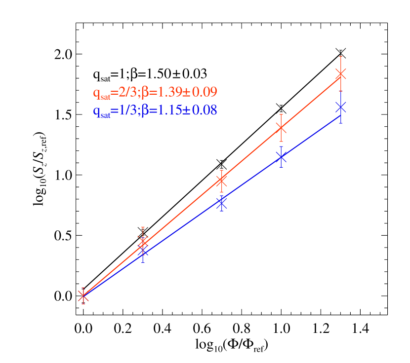
Figure 12: Effect of quenching of horizontal motions by strong magnetic field. We show the relation of the quenched Poynting flux $\widetilde{S}_{z}$ as defined in Eq. (33) to the unsigned surface magnetic flux $\Phi$. Each data point represents an average in time and space for each run. The values are normalized to model run 1B represented here by the subscript ’ref’. The black line shows the power-law fit to the case where no quenching is included (i.e. $q_{\rm{sat}}=1$). The red and blue lines show power-law fits for $q_{\rm{sat}}=2/3$ and 1/3. The corresponding power-law indices $\beta$ for $\widetilde{S}_{z}\propto\Phi^{\,\beta}$ are given with the legend.

In general, the Poynting flux is defined as

$$S_{z}=\eta(\bm{j}\times\bm{B})\big{|}_{z}-\frac{1}{\mu_{0}}(\bm{u}\times\bm{B}\times\bm{B})\big{|}_{z}.$$ (31)

The first term $\bm{j}\times\bm{B}$ is not affected by the quenching of horizontal motions. The second term can be further decomposed into two terms,

$$\bm{u}\times\bm{B}\times\bm{B}\big{|}_{z}\leavevmode\nobreak\ =\leavevmode\nobreak\ u_{z}\,B^{2}_{\rm h}\leavevmode\nobreak\ -\leavevmode\nobreak\ B_{z}\,B_{\rm h}\,u^{\prime}_{\rm h},$$ (32)

where we now use the horizontal velocities quenched by the magnetic field, $u^{\prime}_{\rm h}$. The subscript h refers to horizontal component combining the $x$ and $y$ direction. From the two terms in Eq. (32) the first term is less relevant in our context, because the vertical velocities are smaller than the horizontal ones at the surface, and because the horizontal magnetic field is smaller than the vertical one. Only the second term,

$$\widetilde{S}_{z}=\frac{1}{\mu_{0}}\leavevmode\nobreak\ B_{z}\,B_{\rm h}\,u^{\prime}_{\rm h},$$ (33)

will be affected by quenching of the horizontal velocities and is of foremost interest in the discussion in this Appendix.

To test the effect of the quenching of the horizontal motions on the Poynting flux we therefore evaluate $\widetilde{S}_{z}$ from Eq. (33). To this end, we calculate the quenching term $q$ as defined in Eq. (30) at each location at the bottom boundary, i.e., the surface, calculate the quenched velocity according to Eq. (29), and then derive the vertical component of the Poynting flux due to the quenched horizontal motions, $\widetilde{S}_{z}$, at the bottom boundary of our model runs. As done for the other (average) quantities in our study, the quenched Poynting flux at the bottom is (horizontally) averaged in space and in time during the relaxed state of the simulations. For better comparison between the different models, we normalize the (average) magnetic flux and Poynting flux at the bottom by the respective values from model run 1B.

To quantify the effect of the quenching on the scaling between magnetic flux $\Phi$ and Poynting flux at the surface $\widetilde{S}_{z}$, we conduct experiments for three cases with $q_{\rm{sat}}=1$, 2/3, and 1/3. These experiments are illustrated in Fig. 12. For the case with no quenching ($q_{\rm{sat}}{=}1$), we find a power-law scaling $\widetilde{S}_{z}\propto\Phi^{\,\beta}$ with a power-law index $\beta=1.5$. This is slightly smaller than $\beta$ in the full model in Fig. 7 and Eq. (18), but still within the range of uncertainties given there. The small difference is because of neglecting the other terms of the Poynting flux in Eq. (31) and because in the main text we consider the Poynting flux at the base of the corona (see Sect. 6.1) and not at the bottom boundary as done here. More importantly, the power-law relation $\widetilde{S}_{z}\propto\Phi^{\,\beta}$ gets more shallow for stronger quenching, with the power-law index $\beta$ going down to about 1.4 and 1.15 for values of $q_{\rm{sat}}$ of 2/3 and 1/3. Consequently, for a more realistic setup with a quenching similar to Gudiksen & Nordlund (2005a), i.e., $q_{\rm{sat}}=1/3$, we would find a reduction of the power-law index $\beta$ by about 25% compared to the case of no quenching.

The reduction of the power-law index $\beta$ by the quenching of horizontal motions will also affect how the X-ray luminosity $L_{\rm{X}}$ scales with the surface magnetic flux $\Phi$. In the framework of the analytical model in Sect. 6.4, the power-law index $m$ of $L_{\rm{X}}\propto\Phi^{m}$ is expressed in Eq. (25) as a function of three parameters, $\alpha,\beta,\gamma$, of which only the parameter $\beta$ will be affected by the quenching. $\alpha$ and $\gamma$ will retain the values discussed in Sect. 6.4. Following Eq. (25), $m$ is linear in $\beta$. Hence its reduction through the quenching for a more realistic setup would be the same as for $\beta$, that is, about 25%. Therefore we would expect the quenching to reduce $m$ as found in our numerical experiments as displayed in Fig. 9 and discussed in Sect. 6.3 to about $m=2.6$. This would be very close to the value of 2.68 found by Kochukhov et al. (2020) in their recent observational study, but still considerably higher than the traditional value that is assumed to be not considerably higher than unity (Fisher et al. 1998; Pevtsov et al. 2003).