Stability study of a model for the Klein-Gordon equation in Kerr space-time II

Abstract

The present paper is a follow-up of our previous paper that derives a slightly simplified model equation for the Klein-Gordon equation, describing the propagation of a scalar field of mass $\mu$ in the background of a rotating black hole and, among others, supports the instability of the field down to $a/M\approx 0.97$. The latter result was derived numerically. This paper gives corresponding rigorous results, supporting instability of the field down to $a/M\approx 0.979796$.

1 Introduction

The question of the stability of the solutions of the Klein-Gordon equation, describing a massive scalar field inside the gravitational field of rotating (Kerr-) black hole, (in Boyer-Lindquist coordinates,) is an important model problem, in view of the stability of the Kerr metric. Results of Damour, Deruelle and Ruffini ([13], 1976), of Zouros and Eardley ([42], 1979) and Detweiler ([14], 1980) indicate the existence of unstable modes for ‘small’ masses of the black hole. This is a surprising result because the Klein-Gordon equation, describing a massive field, is a perturbation of the wave equation on Kerr background, by a positive potential. Intuitively, it might be expected that such perturbations stabilize solutions, and the solutions of the latter equation are indeed stable [40, 18, 12, 37]. The rigorous proof of the results above was of considerable interest, since, if true, this could indicate that infalling matter destabilizes Kerr black holes. Beyer ([8], 2011) proves that the restrictions of the solutions of the separated, in the azimuthal coordinate, Klein-Gordon field are stable for sufficiently large masses $\mu>0$ of the field.

$$\mu\geqslant\frac{|m|a}{2Mr_{+}}\sqrt{1+\frac{2M}{r_{+}}}\,\,.$$ (1.0.1)

Here $M>0$ is the mass of the black hole, $0\leqslant a<M$ is the rotational parameter, $m\in{\mathbb{Z}}$ is the ‘azimuthal separation parameter’ and

$$r_{+}:=M+\sqrt{M^{2}-a^{2}}\,\,.$$

The result is consistent with [13], but contradicts results of [42]. A numerical investigation by Furuhashi and Nambu ([19], 2004) finds unstable modes for $\mu M\sim 1$ and $(a/M)=0.98$. A numerical investigation by Cardoso et al. ([11], 2004), finds unstable modes for $\mu M\leqslant 1$ and $0.98\leqslant(a/M)<1$. A numerical investigation by Strafuss and Khanna ([24], 2005) finds unstable modes for $\mu M\sim 1$ and $(a/M)=0.9999$. A numerical investigation by Konoplya and Zhidenko ([27], 2006) confirms the results of Beyer ([4], 2001, [8], 2011). In addition, no unstable modes are found also for $\mu M\ll 1$ and $\mu M\sim 1$. ($0\leqslant a\leqslant 0.995)$. The latter result contradicts, in particular, analytical results from Detweiler [14]. An analytical study by Hod and Hod ([22], 2010) finds unstable modes for $\mu M\sim 1$ with a growth rate,

$$1.7\cdot 10^{-3}M^{-1}\,\,,$$

which is four orders of magnitude larger than previously estimated.
There was a mounting evidence that the solutions of the Klein-Gordon equation on a Kerr background are unstable, if the estimate (1.0.1) is violated. By negelecting “small” terms, in the sense of the used operator-theoretic methods, Beyer, Alcubierre & Megevand, ([9], 2013) create a spherically symmetric model equation that is closely related to the Klein-Gordon equation on a Kerr background and whose modes can be expressed in terms of Coulomb wave functions. Analogous to the Klein-Gordon equation on a Kerr background, the model equation is of the form

$$(u^{\prime})^{\prime}(t)+iBu^{\prime}(t)+Au(t)=0\,\,,$$ (1.0.2)

for every $t\in{\mathbb{R}}$, where $u$ is the unknown function, assuming values in a weighted $L^{2}$-space $X$, $A$ is a densely-defined, linear and self-adjoint operators in $X$ and $B$ is a bounded linear and self-adjoint operator in $X$. The operators $A$ and $B$ do not commute, as is the case also for the Klein-Gordon equation on a Kerr background. The stability of the solutions of (1.0.2) is governed by the spectrum of the corresponding operator polynomial

$$A-\lambda B-\lambda^{2}$$ (1.0.3)

where $\lambda\in{\mathbb{C}}$, i.e., by those $\lambda\in{\mathbb{C}}$, for which the operator in (1.0.3) is not bijective. The solutions of the model equation are unstable down to rotational parameters $a/M\approx 0.9718$. Subsequently, Shlapentokh-Rothman, ([36], 2014) proved the instability of the solutions of the Klein-Gordon equation, describing a massive scalar field on a Kerr background, in the following sense. For each choice of $m\in{\mathbb{Z}}^{*}$, there is a countable family of intervals of masses $\mu$ associated to exponentially growing solutions (indexed by $l\in\{|m|,|m|+1,\dots\}$). These intervals have an accumulation point at

$$\frac{|m|a}{2Mr_{+}}\,\,.$$ (1.0.4)

In addition, these unstable modes exhibit superradiance, i.e., the corresponding frequency $\omega$ satisfies the inequality

$$ma\,{\textrm{Re}}(\omega)-2Mr_{+}|\omega|^{2}>0\,\,.$$

Still, there is very much an implicit dependence on $a/M$, as in the numerical results. The precise dependence of the instability on the parameters, including the value of $a/M$ triggering the onset of the instability is not yet clear.
The present paper is a follow-up of our paper [9]. It continues the study of our model problem, with the purpose of shedding some light on the dependence of the instability on the parameters, including the value of $a/M$ triggering the onset of the instability. Here, it needs to be taken into account that [9] reduces the finding of unstable modes of (1.0.2) to the finding of the solutions of a quartic inside the subset

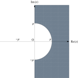
Fig. 1: Sketch of the subset $\Omega_{1}$ of the complex plane.

$$\Omega_{1}:=({\mathbb{C}}\setminus B_{\mu}(0))\cap((0,\infty)\times{\mathbb{R}})$$ (1.0.5)

of the complex plane, but finds these solutions only numerically. Here, ${\mathbb{C}}$ denotes the field of complex numbers, $B_{\mu}(0)$ denotes the closed ball of radius $\mu$ around $0$ and $(0,\infty)\times{\mathbb{R}}$ denotes the open right half-plane. The present paper focuses on obtaining analytical information on these solutions. For the study of the model problem, we assume throughout that

$$M>0\,\,,\,\,0<a<M\,\,,\,\,\mu>0\,\,,\,\,m\in{\mathbb{Z}}\,\,,\,\,l\in\{|m|,|m|+1,\dots\}\,\,.$$

The following is Lemma 3.19 in [9], reducing the finding of unstable modes of (1.0.2) to the solution of a quartic equation and providing the starting point of the investigation.

Lemma 1.1.

If $R=r_{+}$, i.e., $R_{-}=2(M^{2}-a^{2})^{1/2}$, and $\lambda$ satisfies the condition

$$\lambda\neq-\,\frac{1}{2Mr_{+}}\,[ma+ik(M^{2}-a^{2})^{1/2}]\,\,,$$ (1.0.6)

where $k\in{\mathbb{Z}}$, then $\lambda\in{\mathbb{R}}\times(-\infty,0)$ is such that $\ker(A-\lambda B-\lambda^{2})$ is non-trivial if and only if

$$\lambda=-\,\frac{i}{2z}\,(z^{2}-\mu^{2})\,\,,$$

where $z\in\Omega_{1}$ satisfies

$$z^{4} +\frac{(2n+1)(M^{2}-a^{2})^{1/2}+ima}{M(2r_{+}+M)}\,z^{3}+\frac{c_{l}-2M^{2}\mu^{2}}{M(2r_{+}+M)}\,z^{2}$$

$$+\frac{(2n+1)(M^{2}-a^{2})^{1/2}+ima}{M(2r_{+}+M)}\,\mu^{2}z+\frac{M}{2r_{+}+M}\,\mu^{4}=0\,\,,$$ (1.0.7)

for some $n\in{\mathbb{N}}$ and where $c_{l}:=l(l+1)$.

We note that if $z\in\Omega_{1}$ satisfies (1.0.7), then $z^{*}$ is a solution of (1.0.7), where $m$ is replaced by $-m$, that is contained in $\Omega_{1}$. Further, we note that the coefficients of the first and third power of $z$ of the quartic (1.0.7) are neither real nor purely imaginary, if $m\neq 0$. The remaining coefficients are real. For the model problem, there is a stability condition given by (1.0.8) from Corollary 3.16 of [9]:

Corollary 1.2.

If $R=r_{+}$, i.e., $R_{-}=2(M^{2}-a^{2})^{1/2}$,

$$\mu^{2}\leq\frac{l(l+1)}{2M(r_{+}+2M)}\,\,,$$ (1.0.8)

and $\lambda\in{\mathbb{C}}\setminus{\mathbb{R}}$ satisfies the condition (1.0.6), then $\ker(A-\lambda B-\lambda^{2})$ is trivial.

As a consequence, for the case $m=0$, $\ker(A-\lambda B-\lambda^{2})$ is trivial. Hence, in the following, we assume throughout that

$$m\in{\mathbb{Z}}^{*}\,\,.$$

In following sections, we proceed to show the existence of solutions of (1.0.7) inside $\Omega_{1}$, and hence the existence of unstable modes in a subregion of the parameter space. Although the roots of any forth degree polynomial, such as that in (1.0.7), are known explicitly, the expressions, seen as functions of all the parameters involved (i.e. $a$, $\mu$, $n$, $l$ and $m$), are too complicated to get any intuitive understanding of the problem just from their analytical form. Thus, we are using other analytical methods for determining the location of the roots, in particular, Routh-Hurwitz criteria, for the localization of roots in half-planes, the Schur-Cohn algorithm, for the localization of roots inside the closed unit disk, Rouche’s theorem, for the localization of roots in general domains, calculation of discriminants of polynomials and direct estimates. We give $2$ approaches. Approach 1 shows the existence of roots in (1.0.5), for sufficiently large $a/M$, without giving a lower bound for $a/M$. Approach 2 shows the existence of roots in (1.0.5), for $a/M$ satisfying the inequality (3.0.4).

2 Approach 1

In the following, we use conformal transformations to transform $\Omega_{1}$ into a subset ($\Omega_{2}$, see (2.0.4)) of the complex plane that is suitable, for the application, in particular, of the Schur-Cohn algorithm. We note by $P$ the polynomial in (1.0.7), i.e.,

$$P(z):=z^{4} +\frac{(2n+1)(M^{2}-a^{2})^{1/2}+ima}{M(2r_{+}+M)}\,z^{3}+\frac{c_{l}-2M^{2}\mu^{2}}{M(2r_{+}+M)}\,z^{2}$$

$$+\frac{(2n+1)(M^{2}-a^{2})^{1/2}+ima}{M(2r_{+}+M)}\,\mu^{2}z+\frac{M}{2r_{+}+M}\,\mu^{4}\,\,,$$

for every $z\in{\mathbb{C}}$. Then,

$$\frac{P(z)}{\mu^{4}}=\left(i\,\frac{z}{\mu}\right)^{4}-\frac{ma-i(2n+1)(M^{2}-a^{2})^{1/2}}{\mu M(2r_{+}+M)}\,\left(i\,\frac{z}{\mu}\right)^{3}$$

$$+\frac{2M^{2}\mu^{2}-l(l+1)}{\mu^{2}M(2r_{+}+M)}\,\left(i\,\frac{z}{\mu}\right)^{2}$$

$$+\frac{ma-i(2n+1)(M^{2}-a^{2})^{1/2}}{\mu M(2r_{+}+M)}\,\left(i\,\frac{z}{\mu}\right)+\frac{M}{2r_{+}+M}\,\,,$$

and hence

$$P(z)=\mu^{4}f\left(i\,\frac{z}{\mu}\right)\,\,,$$

for every $z\in{\mathbb{C}}$, where

Definition 2.1.

(Definition of $f$) We define $f:{\mathbb{C}}\rightarrow{\mathbb{C}}$ by

$$f(u) :=u^{4}-\frac{ma-i(2n+1)(M^{2}-a^{2})^{1/2}}{\mu M(2r_{+}+M)}\,u^{3}+\frac{2M^{2}\mu^{2}-l(l+1)}{\mu^{2}M(2r_{+}+M)}\,u^{2}$$

$$\quad\,\,\,+\frac{ma-i(2n+1)(M^{2}-a^{2})^{1/2}}{\mu M(2r_{+}+M)}\,u+\frac{M}{2r_{+}+M}\,\,,$$ (2.0.1)

for every $u\in{\mathbb{C}}$.

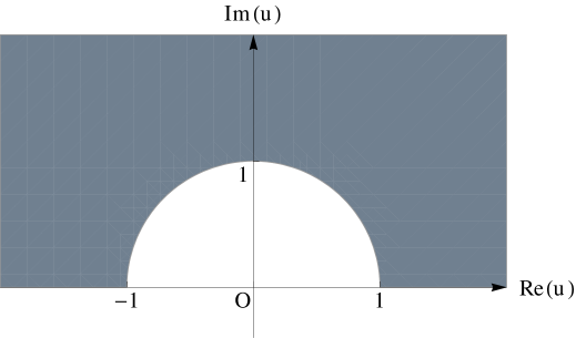
Fig. 2: The domain of values of $u$ inside the domain of $f$, leading on unstable $\lambda$ is given by the complement of the upper closed half-disk, shaded in gray.

.

As a consequence, we arrive at the following:

Lemma 2.2.

(Instability in terms of roots of $f$) If $R=r_{+}$, i.e., $R_{-}=2(M^{2}-a^{2})^{1/2}$, and $\lambda$ satisfies (1.0.6), then $\lambda\in{\mathbb{R}}\times(-\infty,0)$ is such that $\ker(A-\lambda B-\lambda^{2})$ is non-trivial if and only if

$$\lambda=-\frac{\mu}{2u}\,(1+u^{2})=-\frac{\mu}{2}\left(u+\frac{1}{u}\right)\,\,,$$

for a root $u$ of $f$ contained in $({\mathbb{C}}\setminus B_{1}(0))\cap({\mathbb{R}}\times(0,\infty))$.

We note that

$$\left(U_{1}(0)\cap({\mathbb{R}}\times(-\infty,0))\rightarrow({\mathbb{C}}\setminus B_{1}(0))\cap({\mathbb{R}}\times(0,\infty)),u\mapsto\frac{1}{u}\,\right)$$

is biholomorphic. Further, for $w\in U_{1}(0)\cap({\mathbb{R}}\times(-\infty,0))$, it follows that

$$f(w^{-1}) =w^{-4}-\frac{ma-i(2n+1)(M^{2}-a^{2})^{1/2}}{\mu M(2r_{+}+M)}\,w^{-3}+\frac{2M^{2}\mu^{2}-l(l+1)}{\mu^{2}M(2r_{+}+M)}\,w^{-2}$$

$$\quad\,\,\,+\frac{ma-i(2n+1)(M^{2}-a^{2})^{1/2}}{\mu M(2r_{+}+M)}\,w^{-1}+\frac{M}{2r_{+}+M}$$

$$=w^{-4}\left[1-\frac{ma-i(2n+1)(M^{2}-a^{2})^{1/2}}{\mu M(2r_{+}+M)}\,w+\frac{2M^{2}\mu^{2}-l(l+1)}{\mu^{2}M(2r_{+}+M)}\,w^{2}\right.$$

$$\left.\qquad\quad\,\,\,+\frac{ma-i(2n+1)(M^{2}-a^{2})^{1/2}}{\mu M(2r_{+}+M)}\,w^{3}+\frac{M}{2r_{+}+M}\,w^{4}\right]\,\,.$$

As a consequence, we define the following.

Definition 2.3.

(Definition of $p,p_{e}$ and $\delta$) We define,

$$p(w) :=w^{4}+\frac{ma-i(2n+1)(M^{2}-a^{2})^{1/2}}{\mu M^{2}}\,w^{3}$$ (2.0.2)

$$\quad\,\,\,+\frac{2M^{2}\mu^{2}-l(l+1)}{\mu^{2}M^{2}}\,w^{2}-\frac{ma-i(2n+1)(M^{2}-a^{2})^{1/2}}{\mu M^{2}}\,w+\frac{2r_{+}+M}{M}\,\,,$$

$$\,\,=w^{4}+\frac{\frac{ma}{M}-i(2n+1)\sqrt{1-\frac{a^{2}}{M^{2}}}}{\mu M}\,w(w^{2}-1)$$

$$\quad\,\,\,+\left[2-\frac{l(l+1)}{\mu^{2}M^{2}}\right]w^{2}+3+2\sqrt{1-\frac{a^{2}}{M^{2}}}\,\,,$$

$$\,\,=w^{4}+\frac{m-m\left(1-\frac{a}{M}\right)-i(2n+1)\sqrt{1-\frac{a^{2}}{M^{2}}}}{\mu M}\,w(w^{2}-1)$$

$$\quad\,\,\,+\left[2-\frac{l(l+1)}{\mu^{2}M^{2}}\right]w^{2}+3+2\sqrt{1-\frac{a^{2}}{M^{2}}}\,\,,$$

$$\,\,=w^{4}+\frac{m}{\mu M}\,w(w^{2}-1)+\left[2-\frac{l(l+1)}{\mu^{2}M^{2}}\right]w^{2}+3$$

$$\quad\,\,\,\,-\frac{m\left(1-\frac{a}{M}\right)+i(2n+1)\sqrt{1-\frac{a^{2}}{M^{2}}}}{\mu M}\,w(w^{2}-1)+2\sqrt{1-\frac{a^{2}}{M^{2}}}\,\,,$$

$$=p_{e}(w)+\delta(w)\,\,,$$

for every $w\in{\mathbb{C}}$, where

$$p_{e}(w) :=w^{4}+\frac{m}{\mu M}\,w(w^{2}-1)+\left[2-\frac{l(l+1)}{\mu^{2}M^{2}}\right]w^{2}+3\,\,,$$ (2.0.3)

$$\delta(w) :=-\frac{m\left(1-\frac{a}{M}\right)}{\mu M}\,w(w^{2}-1)+2\,\sqrt{1-\frac{a^{2}}{M^{2}}}\left[1-i\,\frac{2n+1}{2\mu M}\,\,w(w^{2}-1)\right]\,\,,$$

for every $w\in{\mathbb{C}}$.

Hence, we arrive at the following

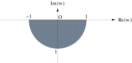
Fig. 3: The domain of values of $w$ inside the domain of $p$, leading on unstable $\lambda$ is given by the lower open half disk, shaded in gray.

.

Lemma 2.4.

(Instability in terms of roots of $p$) If $R=r_{+}$, i.e., $R_{-}=2(M^{2}-a^{2})^{1/2}$, and $\lambda$ satisfies (1.0.6), then $\lambda\in{\mathbb{R}}\times(-\infty,0)$ is such that $\ker(A-\lambda B-\lambda^{2})$ is non-trivial, if and only if

$$\lambda=-\frac{\mu}{2w}\,(1+w^{2})=-\frac{\mu}{2}\left(w+\frac{1}{w}\right)\,\,,$$

for a root $w$ of $p$ contained in

$$\Omega_{2}:=U_{1}(0)\cap({\mathbb{R}}\times(-\infty,0))\,\,.$$ (2.0.4)

We note that

$$p_{e}(w)=w^{4}+{\alpha}w^{3}+({\beta}-4)w^{2}-{\alpha}w+3\,\,,$$

where

$$\alpha=\frac{m}{\mu M}\,\,,\,\,\beta=6-\frac{l(l+1)}{\mu^{2}M^{2}}\,\,,$$

are dimensionless. Also, we note that, since

$$\frac{l(l+1)}{6M^{2}}\geqslant\frac{l(l+1)}{2M(3M+\sqrt{M^{2}-a^{2}}\,)}=\frac{l(l+1)}{2M(r_{+}+2M)}\,\,,$$

the condition that

$$\mu^{2}>\frac{l(l+1)}{6M^{2}}\,\,,$$

implies that

$$\mu^{2}>\frac{l(l+1)}{2M(r_{+}+2M)}\,\,.$$

More generally, in the following, we define for $\alpha,\beta\in{\mathbb{R}}$ the polynomial $q$ by

$$q_{\alpha,\beta}(w):=w^{4}+{\alpha}w^{3}+({\beta}-4)w^{2}-{\alpha}w+3\,\,,$$ (2.0.5)

for every $w\in{\mathbb{C}}$. As a consequence, if

$$\alpha=\frac{m}{\mu M}\,\,,\,\,\beta=6-\frac{l(l+1)}{\mu^{2}M^{2}}\,\,,$$

then

$$p_{e}=q_{\alpha,\beta}\,\,.$$

In the following, we are going to apply the Cohn-Schur algorithm to find the number of roots of $q_{(\alpha,\beta)}$ in the open ball of radius $1$ around the origin, $U_{1}(0)$, of the complex plane.

Theorem 2.5.

(Number of roots of $q_{\alpha,\beta}$ inside $U_{1}(0)$) Let $\alpha,\beta\in{\mathbb{R}}$ be such that

$$4<\alpha^{2}\,\,,\,\,0<\beta\,\,.$$

Then $q_{\alpha,\beta}$ has $2$ roots inside $U_{1}(0)$, where multiple roots are counted with their multiplicity.

Proof.

In the following, we are going to apply Theorem 6.8c of [20]. Here $T^{k}q_{\alpha,\beta}$, $k=1,\dots,4$, denote the iterated Schur transforms of $q_{\alpha,\beta}$, a $*$ indicates a reciprocal polynomial and $\gamma_{k}:=(T^{k}q_{\alpha,\beta})(0)$, for $k=1,\dots,4$. It follows for every $w\in{\mathbb{C}}$ that

$$q_{\alpha,\beta}(w) =w^{4}+{\alpha}w^{3}+({\beta}-4)w^{2}-{\alpha}w+3\,\,,$$

$$q_{\alpha,\beta}^{*}(w) =3w^{4}-{\alpha}w^{3}+({\beta}-4)w^{2}+{\alpha}w+1\,\,,$$

$$(Tq_{\alpha,\beta})(w) =3q_{\alpha,\beta}(w)-q_{\alpha,\beta}^{*}(w)$$

$$=3w^{4}+3{\alpha}w^{3}+3({\beta}-4)w^{2}-3aw+9$$

$$\quad\,-[3w^{4}-{\alpha}w^{3}+({\beta}-4)w^{2}+{\alpha}w+1]$$

$$=4{\alpha}w^{3}+2({\beta}-4)w^{2}-4{\alpha}w+8$$

$$(Tq_{\alpha,\beta})^{*}(w) =8w^{3}-4{\alpha}w^{2}+2({\beta}-4)w+4\alpha\,\,$$

$$(T^{2}q_{\alpha,\beta})(w) =8(Tq_{\alpha,\beta})(w)-4\alpha(Tq_{\alpha,\beta})^{*}(w)$$

$$=8[4{\alpha}w^{3}+2({\beta}-4)w^{2}-4{\alpha}w+8]$$

$$\quad-4{\alpha}[8w^{3}-4{\alpha}w^{2}+2({\beta}-4)w+4\alpha]$$

$$=16({\alpha}^{2}+{\beta}-4)w^{2}-8{\alpha}[4+({\beta}-4)]w+16(4-{\alpha}^{2})$$

$$=16({\alpha}^{2}+{\beta}-4)w^{2}-8{\alpha}{\beta}w+16(4-{\alpha}^{2})\,\,,$$

$$(T^{2}q_{\alpha,\beta})^{*}(w) =16(4-{\alpha}^{2})w^{2}-8{\alpha}{\beta}w+16({\alpha}^{2}+{\beta}-4)\,\,,$$

$$(T^{3}q_{\alpha,\beta})(w) =16(4-{\alpha}^{2})[16({\alpha}^{2}+{\beta}-4)w^{2}-8{\alpha}{\beta}w+16(4-{\alpha}^{2})]$$

$$\quad\,-16({\alpha}^{2}+{\beta}-4)[16(4-{\alpha}^{2})w^{2}-8{\alpha}{\beta}w+16({\alpha}^{2}+{\beta}-4)]$$

$$=128{\alpha}{\beta}[2({\alpha}^{2}-4)+{\beta}]w+256[(4-{\alpha}^{2})^{2}-({\alpha}^{2}-4+{\beta})^{2}]$$

$$=128{\alpha}{\beta}[2({\alpha}^{2}-4)+{\beta}]w+256{\beta}[2(4-{\alpha}^{2})-{\beta}]$$

$$=128{\beta}[2({\alpha}^{2}-4)+{\beta}](\alpha w-2)\,\,,$$

$$(T^{3}q_{\alpha,\beta})^{*}(w) =128{\beta}[2({\alpha}^{2}-4)+{\beta}](-2w+\alpha)\,\,,$$

$$(T^{4}q_{\alpha,\beta})(w) =-256{\beta}[2({\alpha}^{2}-4)+{\beta}]\cdot 128{\beta}[2({\alpha}^{2}-4)+{\beta}](\alpha w-2)$$

$$\quad\,-128{\beta}{\alpha}[2({\alpha}^{2}-4)+{\beta}]\cdot 128{\beta}[2({\alpha}^{2}-4)+{\beta}](-2w+\alpha)$$

$$=-128\cdot 256{\beta}^{2}[2({\alpha}^{2}-4)+{\beta}]^{2}(\alpha w-2)$$

$$\quad\,-128^{2}{\beta}^{2}\alpha[2({\alpha}^{2}-4)+{\beta}]^{2}(-2w+\alpha)$$

$$=256^{2}{\beta}^{2}[2({\alpha}^{2}-4)+{\beta}]^{2}-128^{2}{\beta}^{2}\alpha^{2}[2({\alpha}^{2}-4)+{\beta}]^{2}$$

$$=128^{2}(4-\alpha^{2}){\beta}^{2}[2({\alpha}^{2}-4)+{\beta}]^{2}\,\,,$$

$$\gamma_{1} =8\,\,,$$

$$\gamma_{2} =-16({\alpha}^{2}-4)\,\,,$$

$$\gamma_{3} =-2\cdot 128{\beta}[2({\alpha}^{2}-4)+{\beta}]\,\,,$$

$$\gamma_{4} =-128^{2}({\alpha}^{2}-4){\beta}^{2}[2({\alpha}^{2}-4)+{\beta}]^{2}\,\,.$$

As a consequence, we conclude that the conditions

$${\alpha}^{2}>4\,\,\wedge\,\,{\beta}>0$$

imply that

$$\gamma_{1}>0\,\,,\,\,\gamma_{2}<0\,\,,\,\,\gamma_{3}<0\,\,,\,\,\gamma_{4}<0$$

and hence that the corresponding indices $k_{1},k_{2},k_{3}$ are given by

$$k_{1}=2\,\,,\,\,k_{2}=3\,\,,\,\,k_{3}=4\,\,.$$

Therefore, according to Theorem 6.8c of [20], the number of roots of $q_{\alpha,\beta}$ in $U_{1}(0)$, multiple roots counted with their multiplicity, is given by

$$\sum_{j=1}^{3}(-1)^{j-1}(4+1-k_{j}) =5-k_{1}-(5-k_{2})+5-k_{3}=5-2-(5-3)+5-4$$

$$=3-2+1=2\,\,.$$

∎

In the next step, we calculate the discriminant of the polynomial $q_{\alpha,\beta}$, to obtain information on the multiplicities of the roots of $q_{\alpha,\beta}$.

Theorem 2.6.

(Calculation of the discriminant of $q_{\alpha,\beta}$) Let $\alpha,\beta\in{\mathbb{R}}$ be such that

$$4<\alpha^{2}<6\,\,,\,\,\frac{4}{100}<\beta<\frac{165}{100}\,\,.$$

Then $q_{\alpha,\beta}$

• has $4$ pairwise different roots,

• $2$ of these roots are real,

• and $2$ of these roots are non-real and conjugate complex.

Proof.

From direct calculation, it follows that the discriminant $\triangle$ of $q_{\alpha,\beta}$ is given by

$$\triangle =4{\alpha}^{6}+{\alpha}^{4}{\beta}^{2}-80{\alpha}^{4}{\beta}+16{\alpha}^{4}-16{\alpha}^{2}{\beta}^{3}+432{\alpha}^{2}{\beta}^{2}-960{\alpha}^{2}{\beta}-320{\alpha}^{2}$$

$$\quad\,+48{\beta}^{4}-768{\beta}^{3}+3456{\beta}^{2}-3072{\beta}+768\,\,$$

$$=768-320{\alpha}^{2}+16{\alpha}^{4}+4{\alpha}^{6}+(-3072-960{\alpha}^{2}-80{\alpha}^{4}){\beta}$$

$$\quad\,+(3456+432{\alpha}^{2}+{\alpha}^{4}){\beta}^{2}+(-768-16{\alpha}^{2}){\beta}^{3}+48{\beta}^{4}$$

$$=4({\alpha}^{2}-4)^{2}(12+{\alpha}^{2})-16(192+60{\alpha}^{2}+5{\alpha}^{4}){\beta}+(3456+432{\alpha}^{2}+{\alpha}^{4}){\beta}^{2}$$

$$\quad\,-16(48+{\alpha}^{2}){\beta}^{3}+48{\beta}^{4}\,\,.$$

Further, with help of the assumed estimates on $\alpha,\beta$, it follows that.

$$\triangle <288-8192{\beta}+6084{\beta}^{2}-832{\beta}^{3}+48{\beta}^{4}$$

$$=4(72-2048{\beta}+1521{\beta}^{2}-208{\beta}^{3}+12{\beta}^{4})=h({\beta})\,\,,$$

where $h:{\mathbb{R}}\rightarrow{\mathbb{R}}$ is defined by

$$h(x):=4(72-2048x+1521x^{2}-208x^{3}+12x^{4})\,\,,$$

for every $x\in{\mathbb{R}}$. We note that,

$$h^{\prime\prime}(x) =12168-4992x+576x^{2}=24(507-208x+24x)$$

$$=24\left[\left(\sqrt{24}\,x-\frac{104}{\sqrt{24}}\right)^{2}+\frac{169}{3}\right]=(24x-104)^{2}+1352>0\,\,.$$

Hence, $h$ is convex. In addition,

$$h\left(\frac{4}{100}\right)<0\,\,,\,\,h\left(\frac{165}{100}\right)<0$$

and hence

$$h(x)<0\,\,,$$

for every

$$x\in\left(\frac{4}{100},\frac{165}{100}\right)\,\,.$$

As a consequence, $g$ has $4$ pairwise different roots, $2$ of these roots are real, and $2$ of these roots are non-real and conjugate complex. ∎

In the next step, we find real roots of $q_{\alpha,\beta}$, with the help of the intermediate value theorem.

Lemma 2.7.

(Real roots of $q_{\alpha,\beta}$) Let $\alpha,\beta\in{\mathbb{R}}$ such that

$$4<\alpha^{2}<6\,\,,\,\,0<\beta<2$$

and $q_{\alpha,\beta}$ be defined by

$$q_{\alpha,\beta}(w):= \,w^{4}+{\alpha}w^{3}+({\beta}-4)w^{2}-{\alpha}w+3\,\,,$$

$$= \,w^{4}+{\alpha}w(w^{2}-1)+({\beta}-4)w^{2}+3\,\,,$$

for every $w\in{\mathbb{C}}$. Then,

• if $\alpha>0$, then $q_{\alpha,\beta}$ has a root in $(-2,-1)$,

• if $\alpha<0$, then $q_{\alpha,\beta}$ has a root in $(1,2)$.

Proof.

First, we note that

$$q_{\alpha,\beta}(-1)=q_{\alpha,\beta}(1)=\beta>0$$

and that

$$q_{\alpha,\beta}(t) =w^{4}+{\alpha}w(w^{2}-1)+({\beta}-4)w^{2}+3$$

$$=w^{4}-4w^{2}+3+{\alpha}w(w^{2}-1)+{\beta}w^{2}$$

$$\leqslant w^{4}-4w^{2}+3+{\alpha}w(w^{2}-1)+2w^{2}$$

$$=w^{4}-2w^{2}+3+{\alpha}w(w^{2}-1)\,\,,$$

for $w\in{\mathbb{R}}$. Hence, if $\alpha>0$, then $\alpha>2$ and

$$q_{\alpha,\beta}(-2)=16-8+3+\alpha\,(-2)(4-1)=11+6(-\alpha)<11-12=-1<0\,\,.$$

As a consequence, $q_{\alpha,\beta}$ has a root in $(-2,-1)$. Further, if $\alpha<0$, then $\alpha<-2$ and

$$q_{\alpha,\beta}(2)=16-8+3+\alpha\cdot 2(4-1)=11+6\alpha<11-12=-1<0\,\,.$$

As consequence, $q_{\alpha,\beta}$ has a root in $(1,2)$. ∎

Summarizing the obtained information on the roots of $q_{\alpha,\beta}$, we obtain:

Theorem 2.8.

(Roots of $q_{\alpha,\beta}$) Let $\alpha,\beta\in{\mathbb{R}}$ such that

$$4<\alpha^{2}<6\,\,,\,\,\frac{4}{100}<\beta<\frac{165}{100}\,\,.$$

Then $q_{\alpha,\beta}$

• has precisely $1$ simple root in $U_{1}(0)\cap({\mathbb{R}}\times(-\infty,0))$,

• $1$ simple root in $U_{1}(0)\cap({\mathbb{R}}\times(0,\infty))$,

• and $2$ different simple roots on ${\mathbb{R}}\setminus[-1,1]$.

We note that this implies that $q_{\alpha,\beta}$ has no roots on $S^{1}\cup[-1,1]$.

Proof.

According to Theorem 2.5, the number of roots of $q_{\alpha,\beta}$ in $U_{1}(0)$, multiple roots counted with their multiplicity, is given by $2$. Further, according Theorem 2.6, $q_{\alpha,\beta}$

• has $4$ pairwise different roots,

• $2$ of these roots are real,

• and $2$ of these roots are non-real and conjugate complex.

As a consequence, $q_{\alpha,\beta}$ has precisely $2$ different roots in $U_{1}(0)$. Also, according to Lemma 2.7, $q_{\alpha,\beta}$ has $1$ real root in ${\mathbb{R}}\setminus[-1,1]$. From the assumption that $q_{\alpha,\beta}$ has $2$ real roots in $U_{1}(0)$, it follows that these roots are different and hence that $q_{\alpha,\beta}$ has $3$ pairwise different real roots.$\lightning$ Hence there is a non-real root in $U_{1}(0)$. The assumption that there is no root in $U_{1}(0)\cap\left({\mathbb{R}}\times(-\infty,0)\right)$ leads to the existence of $1$ root in $U_{1}(0)\cap\left({\mathbb{R}}\times(0,\infty)\right)$ and hence, since $q_{\alpha,\beta}$ has real coefficients, to the existence of a root in $U_{1}(0)\cap\left({\mathbb{R}}\times(-\infty,0)\right)$.$\lightning$ Hence, there is a root in $U_{1}(0)\cap\left({\mathbb{R}}\times(-\infty,0)\right)$, and there is also a root in $U_{1}(0)\cap\left({\mathbb{R}}\times(0,\infty)\right)$. As a consequence, the $2$ real roots are contained in ${\mathbb{R}}\setminus(-1,1)$. Since, $q_{\alpha,\beta}(-1)=q_{\alpha,\beta}(1)=\beta>0$, the $2$ real roots are contained in ${\mathbb{R}}\setminus[-1,1]$. We note that this implies that there are no roots on $S^{1}\cup[-1,1]$. ∎

In the final step, we apply Rouché’s theorem, to prove the existence of roots of $p$ in $\Omega_{2}$, of for $a$ sufficiently close to $M$.

Theorem 2.9.

(Roots of $p$) Let

$$\alpha=\frac{m}{\mu M}\,\,,\,\,\beta=6-\frac{l(l+1)}{\mu^{2}M^{2}}\,\,,$$

be such that

$$4<\alpha^{2}<6\,\,,\,\,\frac{4}{100}<\beta<\frac{165}{100}\,\,.$$ (2.0.6)

Then, for $a$ sufficiently close to $M$, there is a root of $p=p_{e}+\delta$ in

$$U_{1}(0)\cap({\mathbb{R}}\times(-\infty,0))\,\,.$$

Proof.

First, according to Theorem 2.8, $p_{e}$ has precisely $1$ simple root in $U_{1}(0)\cap({\mathbb{R}}\times(-\infty,0))$ and no roots in

$$C:=\partial[U_{1}(0)\cap({\mathbb{R}}\times(-\infty,0))]\,\,.$$

Further, we note that for every $w\in B_{1}(0)$:

$$|\,\delta(w)|=\bigg{|}-\frac{m\left(1-\frac{a}{M}\right)}{\mu M}\,w(w^{2}-1)+2\,\sqrt{1-\frac{a^{2}}{M^{2}}}\left[1-i\,\frac{2n+1}{2\mu M}\,\,w(w^{2}-1)\right]\bigg{|}$$

$$\leqslant|\alpha|\cdot|w|\,(\,|w|^{2}+1)\left(1-\frac{a}{M}\right)+2\,\sqrt{1-\frac{a^{2}}{M^{2}}}\left[1+\frac{2n+1}{2\mu M}\,|w|\,(|w|^{2}+1)\right]$$

$$\leqslant 2\sqrt{6}\left(1-\frac{a}{M}\right)+2\,\sqrt{1-\frac{a^{2}}{M^{2}}}\left(1+\frac{2n+1}{\mu M}\right)\,\,.$$

and hence that

$$\|\,\delta|_{B_{1}(0)}\|_{\infty}\leqslant 2\sqrt{6}\left(1-\frac{a}{M}\right)+2\,\sqrt{1-\frac{a^{2}}{M^{2}}}\left(1+\frac{2n+1}{\mu M}\right)\,\,.$$

Even further, since there are no roots of $p_{e}$ in $C$, it follows that

$$\frac{1}{|g_{e}|}\bigg{|}_{C}$$

is continuous function and, since $C$ is compact, that there is $\varepsilon>0$ such that

$$\frac{1}{|g_{e}(w)|}\leqslant\varepsilon\,\,,$$

for every $w\in C$. The latter implies that

$$|g_{e}(w)|\geqslant\frac{1}{\varepsilon}\,\,,$$

for every $w\in C$. Hence for $a/M$ sufficiently close to $1$, it follows that

$$2\sqrt{6}\left(1-\frac{a}{M}\right)+2\,\sqrt{1-\frac{a^{2}}{M^{2}}}\left(1+\frac{2n+1}{\mu M}\right)<\frac{1}{\varepsilon}$$

and hence that

$$|\delta(w)|<|g_{e}(w)|\,\,,$$

for every $w\in C$. Hence for such a case, it follows from Rouché’s theorem that there is a root of $p=p_{e}+\delta$ in $C$. ∎

The following proposition rewrites the inequalities (2.0.8) in terms of the parameters $\mu,M,m$ and $l$.

Proposition 2.10.

If

$$\frac{25}{149}\,l(l+1)<\mu^{2}M^{2}<\frac{20}{87}\,m^{2}\,\,,$$

then

$$4<\alpha^{2}<6\,\,,\,\,\frac{4}{100}<\beta<\frac{165}{100}\,\,,$$

where

$$\alpha=\frac{m}{\mu M}\,\,,\,\,\beta=6-\frac{l(l+1)}{\mu^{2}M^{2}}\,\,.$$

If $l=|m|+k$, where $k\in{\mathbb{N}}$, the interval

$$\left(\,\frac{25}{149}\,l(l+1)\,,\,\frac{20}{87}\,m^{2}\right)$$

is non-empty, iff

$$|m|>\frac{435}{161}\,(k+1)+\sqrt{\left(\frac{435}{161}\right)^{2}(k+1)^{2}+\frac{435}{161}\,k(k+1)}\,\,.$$ (2.0.7)

We note that if $k=0$, (2.0.7) leads to

$$|m|>2\,\frac{435}{161}=\frac{870}{161}\approx 5.40373\,\,.$$

Proof.

Since

$$\alpha=\frac{m}{\mu M}\,\,,\,\,\beta=6-\frac{l(l+1)}{\mu^{2}M^{2}}\,\,,$$

the inequalities

$$4<\alpha^{2}<6\,\,\wedge\,\,\frac{4}{100}<\beta<\frac{165}{100}$$

are equivalent to

$$4<\frac{m^{2}}{\mu^{2}M^{2}}<6\,\,\wedge\,\,\frac{4}{100}<6-\frac{l(l+1)}{\mu^{2}M^{2}}<\frac{165}{100}\,\,.$$ (2.0.8)

We note the equivalence of the following inequalities

$$\frac{4}{100}<6-\frac{l(l+1)}{\mu^{2}M^{2}}<\frac{165}{100}\,\,\Leftrightarrow\,\,-\frac{4}{100}>-6+\frac{l(l+1)}{\mu^{2}M^{2}}>-\frac{165}{100}\,\,,$$

$$6-\frac{4}{100}>\frac{l(l+1)}{\mu^{2}M^{2}}>6-\frac{165}{100}\,\,\Leftrightarrow\,\,\frac{149}{25}>\frac{l(l+1)}{\mu^{2}M^{2}}>\frac{87}{20}\,\,,$$

$$\frac{25}{149}<\frac{\mu^{2}M^{2}}{l(l+1)}<\frac{20}{87}\,\,\Leftrightarrow\,\,\frac{25}{149}\,l(l+1)<\mu^{2}M^{2}<\frac{20}{87}\,l(l+1)$$

as well as

$$4<\frac{m^{2}}{\mu^{2}M^{2}}<6\,\,\Leftrightarrow\,\,\frac{1}{6}<\frac{\mu^{2}M^{2}}{m^{2}}<\frac{1}{4}\,\,\Leftrightarrow\frac{m^{2}}{6}<\mu^{2}M^{2}<\frac{m^{2}}{4}\,\,.$$

Hence, (2.0.8) is equivalent to

$$\frac{25}{149}\,l(l+1)<\mu^{2}M^{2}<\min\left\{\frac{m^{2}}{4},\frac{20}{87}\,l(l+1)\right\}=\min\left\{\frac{m^{2}}{4},\frac{l(l+1)}{4.35}\right\}\,\,,$$

where we used that, since $l\geqslant|m|$,

$$\frac{25}{149}\,l(l+1)\geqslant\frac{25}{149}\,|m|^{2}\geqslant\frac{25}{150}\,|m|^{2}=\frac{m^{2}}{6}\,\,.$$

Since

$$\frac{m^{2}}{4.35}=\min\left\{\frac{m^{2}}{4},\frac{m^{2}}{4.35}\right\}\leqslant\min\left\{\frac{m^{2}}{4},\frac{l(l+1)}{4.35}\right\}\,\,,$$

it follows that the inequality

$$\frac{25}{149}\,l(l+1)<\mu^{2}M^{2}<\frac{20}{87}\,m^{2}$$

implies (2.0.8). If $l=|m|+k$, where $k\in{\mathbb{N}}$, the interval

$$\left(\,\frac{25}{149}\,l(l+1)\,,\,\frac{20}{87}\,m^{2}\right)$$

is non-empty, iff

$$\frac{20}{87}\,m^{2}>\frac{25}{149}\,(|m|+k)(|m|+k+1)\,\,,$$

$$\frac{20}{87}\,m^{2}>\frac{25}{149}\,(|m|+k)(|m|+k+1)=\frac{25}{149}\,[m^{2}+2|m|(k+1)+k(k+1)]\,\,,$$

$$\frac{805}{12963}\,m^{2}>\frac{25}{149}\,[2|m|(k+1)+k(k+1)]\,\,,$$

$$m^{2}>\frac{435}{161}\,[2|m|(k+1)+k(k+1)]\,\,,$$

$$m^{2}-\frac{435}{161}\,[2|m|(k+1)+k(k+1)]>0\,\,,$$

$$\left[|m|-\frac{435}{161}\,(k+1)\right]^{2}-\left(\frac{435}{161}\right)^{2}(k+1)^{2}-\frac{435}{161}k(k+1)>0\,\,,$$

$$\left[|m|-\frac{435}{161}\,(k+1)\right]^{2}>\left(\frac{435}{161}\right)^{2}(k+1)^{2}+\frac{435}{161}\,k(k+1)\,\,.$$

and hence iff

$$|m|>\frac{435}{161}\,(k+1)+\sqrt{\left(\frac{435}{161}\right)^{2}(k+1)^{2}+\frac{435}{161}\,k(k+1)}\,\,.$$

∎

3 Approach 2

Approach 2 uses the subsequent conformal transformation $h$ to transform the open lower half-disk $\Omega_{2}$ onto to the first quadrant $(0,\infty)^{2}$. The roots of $p\circ h^{-1}$ coincide with the roots of the fourth order polynomial $q$, given in Definition 3.0.1. Subsequently, the argument principle is used to derive Theorem 3.6. Lemmatas 3.4 and 3.5 prepare the proof of Theorem 3.6. Theorem 3.7 shows the existence of roots of $p$ in $\Omega_{2}$ for $a/M$ satisfying the inequality (3.0.4), i.e., for values down to about $0.979796$.

Lemma 3.1 (A biholomorphic map from the open lower half-disk onto the open first quadrant).

By

$$h(z):=\frac{1-z}{1+z}\,\,,$$

for every $z\in U_{1}(0)\cap({\mathbb{R}}\times(-\infty,0))$, there is defined a biholomorphic map

$$h:U_{1}(0)\cap({\mathbb{R}}\times(-\infty,0))\rightarrow(0,\infty)^{2}\,\,,$$

with inverse

$$h^{-1}:(0,\infty)^{2}\rightarrow U_{1}(0)\cap({\mathbb{R}}\times(-\infty,0))\,\,,$$

defined by

$$h^{-1}(u)=\frac{1-u}{1+u}\,\,,$$

for every $u\in(0,\infty)^{2}$.

Proof.

If $z\in U_{1}(0)\cap({\mathbb{R}}\times(-\infty,0))$, $x:=\textrm{Re}(z)$ and $y:=\textrm{Im}(z)\,(<0)$, then

$$\frac{1-z}{1+z}=\frac{1-x-iy}{1+x+iy}=\frac{(1-x-iy)(1+x-iy)}{(1+x+iy)(1+x-iy)}$$

$$=\frac{1-x^{2}-y^{2}-2iy}{(1+x)^{2}+y^{2}}\in(0,\infty)^{2}\,\,.$$

Hence by

$$h(z):=\frac{1-z}{1+z}\,\,,$$

for every $z\in U_{1}(0)\cap({\mathbb{R}}\times(-\infty,0))$, there is defined a holomorphic map

$$h:U_{1}(0)\cap({\mathbb{R}}\times(-\infty,0))\rightarrow(0,\infty)^{2}\,\,.$$

Further, if $u\in(0,\infty)^{2}$, $u_{1}:=\textrm{Re}(u)\,(>0)$ and $u_{2}:=\textrm{Im}(u)\,(>0)$, then

$$\frac{1-u}{1+u}=\frac{1-u_{1}^{2}-u_{2}^{2}-2iu_{2}}{(1+u_{1})^{2}+u_{2}^{2}}\in{\mathbb{R}}\times(-\infty,0)\,\,.$$

In addition,

$$\left[\frac{1-u_{1}^{2}-u_{2}^{2}}{(1+u_{1})^{2}+u_{2}^{2}}\right]^{2}+\left[\frac{-2u_{2}}{(1+u_{1})^{2}+u_{2}^{2}}\right]^{2}$$

$$=\frac{(1-u_{1}^{2}-u_{2}^{2})^{2}+4u_{2}^{2}}{[(1+u_{1})^{2}+u_{2}^{2}]^{2}}=\frac{(1-u_{1}^{2}-u_{2}^{2})^{2}+4u_{2}^{2}}{(1+u_{1}^{2}+u_{2}^{2}+2u_{1})^{2}}$$

$$=\frac{(1+u_{1}^{2}+u_{2}^{2})^{2}-4(u_{1}^{2}+u_{2}^{2})+4u_{2}^{2}}{(1+u_{1}^{2}+u_{2}^{2})^{2}+4u_{1}(1+u_{1}^{2}+u_{2}^{2})+4u_{1}^{2}}$$

$$=\frac{(1+u_{1}^{2}+u_{2}^{2})^{2}-4u_{1}^{2}}{(1+u_{1}^{2}+u_{2}^{2})^{2}+4u_{1}(1+u_{1}^{2}+u_{2}^{2})+4u_{1}^{2}}$$

$$<\frac{(1+u_{1}^{2}+u_{2}^{2})^{2}-4u_{1}^{2}}{(1+u_{1}^{2}+u_{2}^{2})^{2}}<\frac{(1+u_{1}^{2}+u_{2}^{2})^{2}}{(1+u_{1}^{2}+u_{2}^{2})^{2}}=1\,\,,$$

and hence

$$\frac{1-u}{1+u}\in U_{1}(0)\,\,.$$

As a consequence, by

$$g(u):=\frac{1-u}{1+u}\,\,,$$

for every $u\in(0,\infty)^{2}$, there is defined a holomorphic map

$$g:(0,\infty)^{2}\rightarrow U_{1}(0)\cap({\mathbb{R}}\times(-\infty,0))\,\,.$$

Further, for every $z\in U_{1}(0)\cap({\mathbb{R}}\times(-\infty,0))$,

$$g(h(z))=g\left(\frac{1-z}{1+z}\right)=\frac{1-\frac{1-z}{1+z}}{1+\frac{1-z}{1+z}}=\frac{1+z-1+z}{1+z+1-z}=\frac{2z}{2}=z$$

as well as

$$h(g(u))=h\left(\frac{1-u}{1+u}\right)=\frac{1-\frac{1-u}{1+u}}{1+\frac{1-u}{1+u}}=\frac{1+u-1+u}{1+u+1-u}=\frac{2u}{2}=u\,\,,$$

for every $u\in(0,\infty)^{2}$. ∎

We note that

$$p(w) =w^{4}+\frac{\frac{ma}{M}-i(2n+1)\sqrt{1-\frac{a^{2}}{M^{2}}}}{\mu M}\,w(w^{2}-1)$$

$$\quad\,\,\,+\left[2-\frac{l(l+1)}{\mu^{2}M^{2}}\right]w^{2}+3+2\sqrt{1-\frac{a^{2}}{M^{2}}}$$

$$=w^{4}+\alpha w\left(w^{2}-1\right)+(\beta-4)w^{2}+3+\epsilon\,\,,$$

for every $w\in\Omega_{2}=U_{1}(0)\cap({\mathbb{R}}\times(-\infty,0))$, where

$$\alpha:=\frac{\frac{ma}{M}-i(2n+1)\sqrt{1-\frac{a^{2}}{M^{2}}}}{\mu M}\,\,,\,\,\beta:=6-\frac{l(l+1)}{\mu^{2}M^{2}}\,\,,\,\,\epsilon:=2\sqrt{1-\frac{a^{2}}{M^{2}}}\,\,(>0)\,\,.$$

In particular,

$$\alpha=\alpha_{1}-i\alpha_{2}\,\,,$$

where

$$\alpha_{1}=\frac{ma}{\mu M^{2}}\,\,,\,\,\alpha_{2}=\frac{2n+1}{\mu M}\,\sqrt{1-\frac{a^{2}}{M^{2}}}\,\,(>0)\,\,.$$

Further, with the help of the biholomorphic map $h$ from Proposition 3.1, it follows that

$$(p\circ h^{-1})(z)$$

$$=\frac{1}{(1+z)^{4}}\left[(\beta+\epsilon)z^{4}+4(2+\alpha+\epsilon)z^{3}+2(16-\beta+3\epsilon)z^{2}+4(2-\alpha+\epsilon)z+1\right]$$

for every $z\in(0,\infty)^{2}$. Hence, we make the following

Definition 3.2.

(Definition of $q$) We define for $\beta\geqslant 0$

$$q(z):=z^{4}+\frac{4z}{\beta+\epsilon}\left[(2+\epsilon)(z^{2}+1)+\alpha(z^{2}-1)\right]+2\,\frac{16-\beta+3\epsilon}{\beta+\epsilon}\,z^{2}+1\,\,,$$ (3.0.1)

for every $z\in{\mathbb{C}}$.

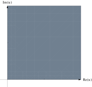
Fig. 4: The domain of values of $u$ inside the domain of $q$, leading on unstable $\lambda$ is given by the open first quadrant, shaded in gray.

.

Lemma 3.3.

(Instability in terms of roots of $q$) If $R=r_{+}$, i.e., $R_{-}=2(M^{2}-a^{2})^{1/2}$, and $\lambda$ satisfies (1.0.6), then $\lambda\in{\mathbb{R}}\times(-\infty,0)$ is such that $\ker(A-\lambda B-\lambda^{2})$ is non-trivial, if and only if

$$\lambda=-\mu\,\frac{1+z^{2}}{1-z^{2}}\,\,,$$

for a root $z$ of $q$ contained in the open first quadrant, $(0,\infty)^{2}$.

Lemma 3.4.

The polynomial $q$ has no real roots. In addition, if

$$\alpha_{1}\geqslant 0\,\,\wedge\,\,0\leqslant\beta\leqslant 16+3\epsilon\,\,,$$

then

$$\lim_{x\rightarrow\infty}\arctan\left(\frac{\textrm{Im}(q(x))}{\textrm{Re}(q(x))}\right)=0\,\,.$$

Proof.

It follows that

$$q(x) =x^{4}+\frac{4x}{\beta+\epsilon}\left[(\epsilon+2)(x^{2}+1)+\alpha(x^{2}-1)\right]+2\,\frac{16-\beta+3\epsilon}{\beta+\epsilon}\,x^{2}+1$$

$$=x^{4}+\frac{4x}{\beta+\epsilon}\left[(\epsilon+2)(x^{2}+1)+\alpha_{1}(x^{2}-1)\right]+2\,\frac{16-\beta+3\epsilon}{\beta+\epsilon}\,x^{2}+1$$

$$\quad\,+i\frac{4\alpha_{2}}{\beta+\epsilon}\,x(1-x^{2})$$

$$=x^{4}+\frac{4x}{\beta+\epsilon}\left\{(\alpha_{1}+\epsilon+2)x^{2}-[\alpha_{1}-(\epsilon+2)]\right\}+2\,\frac{16-\beta+3\epsilon}{\beta+\epsilon}\,x^{2}+1$$

$$\quad\,+i\frac{4\alpha_{2}}{\beta+\epsilon}\,x(1-x^{2})\,\,,$$

for very $x\in{\mathbb{R}}$. We note that $q$ has no real roots. This can be seen as follows. If $x$ is a real root of $q$, then $\textrm{Im}(q(x))=0$ and hence $x\in\{-1,0,1\}$. Further,

$$\textrm{Re}(q(0))=1\neq 0\,\,,$$

$$\textrm{Re}(q(-1))=\textrm{Re}(q(1))$$

$$=1+\frac{4}{\beta+\epsilon}\left\{(\alpha_{1}+\epsilon+2)-[\alpha_{1}-(\epsilon+2)]\right\}+2\,\frac{16-\beta+3\epsilon}{\beta+\epsilon}+1$$

$$=2+\frac{8(\epsilon+2)}{\beta+\epsilon}+2\,\frac{16-\beta+3\epsilon}{\beta+\epsilon}=\frac{2(\beta+\epsilon)}{\beta+\epsilon}+\frac{8(\epsilon+2)}{\beta+\epsilon}+2\,\frac{16-\beta+3\epsilon}{\beta+\epsilon}$$

$$=\frac{2(\beta+\epsilon)+8(\epsilon+2)+2(16-\beta+3\epsilon)}{\beta+\epsilon}=16\,\frac{3+\epsilon}{\beta+\epsilon}\neq 0\,\,.$$

If

$$\alpha_{1}\geqslant 0\,\,\wedge\,\,0\leqslant\beta\leqslant 16+3\epsilon\,\,,$$

then

$$\textrm{Re}(q(x))\geqslant x^{4}+1\,\,,\,\,\text{if $x>1$}$$

as well as

$$\textrm{Im}(q(x))=\frac{4\alpha_{2}}{\beta+\epsilon}\,x(1-x^{2})<0\,\,,\,\,\text{if $x>1$}\,\,,$$

implying that

$$0>\frac{\textrm{Im}(q(x))}{\textrm{Re}(q(x))}\geqslant\frac{4\alpha_{2}}{\beta+\epsilon}\,\frac{x(1-x^{2})}{x^{4}+1}\,\,\text{if $x>1$}$$

and hence that

$$\lim_{x\rightarrow\infty}\frac{\textrm{Im}(q(x))}{\textrm{Re}(q(x))}=0\,\,,\,\,\lim_{x\rightarrow\infty}\arctan\left(\frac{\textrm{Im}(q(x))}{\textrm{Re}(q(x))}\right)=0\,\,.$$

∎

Lemma 3.5.

For

$$\alpha_{1}>2+\epsilon\lor\alpha_{1}<-(2+\epsilon)\,\,,$$

the polynomial $q$ has no purely imaginary roots.

• If

  $$\alpha_{1}>2+\epsilon\,\,,$$

  the function

  $$h_{2}:=({\mathbb{R}}\rightarrow{\mathbb{R}},y\mapsto{\textrm{Im}}(q(iy)))$$

  is strictly decreasing and

  $$h_{2}((0,\infty))\subset(-\infty,0)\,\,.$$

• If

  $$\alpha_{1}<-(2+\epsilon)\,\,,$$

  the function $h_{2}$ is strictly increasing and

  $$h_{2}((0,\infty))\subset(0,\infty)\,\,.$$

• If

  $$0<\beta<8+\epsilon\,\,,$$

  then

  $$h_{1}:=({\mathbb{R}}\rightarrow{\mathbb{R}},y\mapsto{\textrm{Re}}(q(iy)))$$

  has precisely $2$ positive roots $y_{0},y_{1}$, satisfying $0<y_{0}<y_{1}$. In addition,

  $$\begin{cases}h_{1}(y)>0&\text{for $0\leqslant y<{\bar{y}}_{0}$}\\ h_{1}({\bar{y}}_{0})=0\text{}\\ h_{1}(y)<0&\text{for ${\bar{y}}_{0}<y<{\bar{y}}_{1}$}\\ h_{1}({\bar{y}}_{1})=0\text{}\\ h_{1}(y)>0&\text{for $y>{\bar{y}}_{1}$}\end{cases}\,\,.$$

Proof.

It follows that

$$q(iy) =y^{4}-2\,\frac{16-\beta+3\epsilon}{\beta+\epsilon}\,y^{2}+1-\frac{4\alpha_{2}}{\beta+\epsilon}\,y(y^{2}+1)$$

$$\quad\,-i\frac{4y}{\beta+\epsilon}\left[(\epsilon+2)\left(y^{2}-1\right)+\alpha_{1}\left(y^{2}+1\right)\right]$$

$$=\left(y^{2}-\frac{16-\beta+3\epsilon}{\beta+\epsilon}\right)^{2}-\frac{8(8+\epsilon-\beta)(4+\epsilon)}{(\beta+\epsilon)^{2}}-\frac{4\alpha_{2}}{\beta+\epsilon}\,y(y^{2}+1)$$

$$\quad\,\,-i\frac{4y}{\beta+\epsilon}\left[(\alpha_{1}+\epsilon+2)y^{2}+(\alpha_{1}-(\epsilon+2))\right]\,\,,$$

for every $y\in{\mathbb{R}}$. We note that for

$$\alpha_{1}>2+\epsilon\lor\alpha_{1}<-(2+\epsilon)\,\,,$$

$q$ has no purely imaginary roots. This can be seen as follows. If $iy$, where $y\in{\mathbb{R}}$ is a purely imaginary root of $q$, then $\textrm{Im}(q(iy))=0$ and hence $y=0$. On the other hand,

$$\textrm{Re}(q(0))=1\neq 0\,\,.$$

We note, for

$$\alpha_{1}>2+\epsilon\,\,,$$

that the function

$$h_{2}:=({\mathbb{R}}\rightarrow{\mathbb{R}},y\mapsto{\textrm{Im}}(q(iy)))$$

is strictly decreasing, since

$$h_{2}^{\prime}(y)=-\frac{4}{\beta+\epsilon}\left\{\left[\alpha_{1}-(2+\epsilon)\right]+3\left[\alpha_{1}+(2+\epsilon)\right]y^{2}\right\}<0\,\,,$$

for every $y\in{\mathbb{R}}$. Also, it follows for $y>0$, that

$$h_{2}(y)=\textrm{Im}(q(iy))=-\frac{4y}{\beta+\epsilon}\left[(\alpha_{1}+\epsilon+2)y^{2}+(\alpha_{1}-(\epsilon+2))\right]<0\,\,.$$

Analogously, for

$$\alpha_{1}<-(2+\epsilon)\,\,,$$

the function $h_{2}$ is strictly increasing, since

$$h_{2}^{\prime}(y)=-\frac{4}{\beta+\epsilon}\left\{\left[\alpha_{1}-(2+\epsilon)\right]+3\left[\alpha_{1}+(2+\epsilon)\right]y^{2}\right\}>0\,\,,$$

for every $y\in{\mathbb{R}}$. Also, it follows for $y>0$, that

$$h_{2}(y)=\textrm{Im}(q(iy))=-\frac{4y}{\beta+\epsilon}\left[(\alpha_{1}+\epsilon+2)y^{2}+(\alpha_{1}-(\epsilon+2))\right]>0\,\,.$$

We note, for

$$0<\beta<8+\epsilon\,\,,$$

that the function

$$h_{1}:=({\mathbb{R}}\rightarrow{\mathbb{R}},y\mapsto{\textrm{Re}}(q(iy)))$$

is strictly decreasing on

$$I_{1}:=\left(0\,,\sqrt{\frac{16-\beta+3\epsilon}{\beta+\epsilon}}\,\right)\,\,,$$

since

$$h_{1}^{\prime}(y)=4y\left(y^{2}-\frac{16-\beta+3\epsilon}{\beta+\epsilon}\right)-\frac{4\alpha_{2}\left(3y^{2}+1\right)}{\beta+\epsilon}<0\,\,,$$

for every $y\in I_{1}$, where

$$\sqrt{\frac{16-\beta+3\epsilon}{\beta+\epsilon}}=\sqrt{\frac{16+4\epsilon-(\beta+\epsilon)}{\beta+\epsilon}}=\sqrt{\frac{16+4\epsilon}{\beta+\epsilon}-1}>\sqrt{\frac{16+4\epsilon}{8+2\epsilon}-1}=1\,\,.$$

Further, we note that the following inequalities are equivalent:

$$16-\beta+3\epsilon>2\sqrt{2}\sqrt{(4+\epsilon)(8-\beta+\epsilon)}\,\,,$$

$$(16-\beta+3\epsilon)^{2}>8(4+\epsilon)(8-\beta+\epsilon)\,\,,$$

$$[8-\beta+\epsilon+2(4+\epsilon)]^{2}>8(4+\epsilon)(8-\beta+\epsilon)\,\,,$$

$$(8-\beta+\epsilon)^{2}+4(4+\epsilon)(8-\beta+\epsilon)+4(4+\epsilon)^{2}>8(4+\epsilon)(8-\beta+\epsilon)$$

$$(8-\beta+\epsilon)^{2}-4(4+\epsilon)(8-\beta+\epsilon)+4(4+\epsilon)^{2}>0\,\,,$$

$$[8-\beta+\epsilon-2(4+\epsilon)]^{2}>0\,\,.$$

Since

$$y_{j}^{4}-2\,\frac{16-\beta+3\epsilon}{\beta+\epsilon}\,y_{j}^{2}+1=0\,\,,$$

for $j\in\{0,1\}$, where

$$(\,0<\,)\,\,y_{0} :=\sqrt{\frac{16-\beta+3\epsilon-2\sqrt{2}\sqrt{(4+\epsilon)(8-\beta+\epsilon)}}{\beta+\epsilon}}<\sqrt{\frac{16-\beta+3\epsilon}{\beta+\epsilon}}\,\,,$$

$$y_{1} :=\sqrt{\frac{16-\beta+3\epsilon+2\sqrt{2}\sqrt{(4+\epsilon)(8-\beta+\epsilon)}}{\beta+\epsilon}}>\sqrt{\frac{16-\beta+3\epsilon}{\beta+\epsilon}}\,\,,$$

it follows that

$$h_{1}(y_{0})=-\frac{4\alpha_{2}}{\beta+\epsilon}\,y_{0}(y_{0}^{2}+1)<0\,\,,\,\,h_{1}(y_{1})=-\frac{4\alpha_{2}}{\beta+\epsilon}\,y_{1}(y_{1}^{2}+1)<0\,\,.$$

Since $h_{1}(0)=1>0$, there is ${\bar{y}}_{0}\in(0,y_{0})\subset I_{1}$ such that

$$h_{1}({\bar{y}}_{0})=0\,\,.$$

As a consequence of the fact that $h_{1}$ is strictly decreasing on $I_{1}$, it follows that

$$\begin{cases}h_{1}(y)>0&\text{for $0\leqslant y<{\bar{y}}_{0}$}\\ h_{1}({\bar{y}}_{0})=0\text{}\\ h_{1}(y)<0&\text{for $y\in I_{1}$ such that $y>{\bar{y}}_{0}$}\end{cases}\,\,.$$

Since, for $y\in{\mathbb{R}}$,

$$h_{1}(y)=y^{4}-2\,\frac{16-\beta+3\epsilon}{\beta+\epsilon}\,y^{2}+1-\frac{4\alpha_{2}}{\beta+\epsilon}\,y(y^{2}+1)\,\,,$$

for sufficiently large $y>0$, is dominated by the highest power, i.e., $4$, there is $\xi_{1}>y_{1}$, such that $h_{1}(\xi_{1})>0$. Hence there is ${\bar{y}}_{1}\in(y_{1},\xi_{1})$, such that

$$h_{1}({\bar{y}}_{1})=0\,\,.$$

We note that the discriminant $\triangle$ of $h_{1}$ is given by

$$\triangle=\frac{4096}{(\beta+\epsilon)^{6}}\left(8+\epsilon-\beta+2\alpha_{2}\right)\left(8+\epsilon-\beta-2\alpha_{2}\right)\left(8\beta+8\epsilon+2\beta\epsilon+2\epsilon^{2}+\alpha_{2}^{2}\right)^{2}\,\,.$$

Hence, if

$$\alpha_{2}<\frac{1}{2}\,(8+\epsilon-\beta)\,\,,$$

then

$$\triangle>0$$

and $h_{1}$ has only real roots. In these cases Descartes’ rule of signs is exact, see, e.g., Corollary 10.1.12 in [32]. Since,

$$h_{1}(-y)=y^{4}-2\,\frac{16-\beta+3\epsilon}{\beta+\epsilon}\,y^{2}+1+\frac{4\alpha_{2}}{\beta+\epsilon}\,y(y^{2}+1)\,\,,$$

for every $y\in{\mathbb{R}}$, and there are $2$ sign changes in the previous polynomial, this polynomial has precisely $2$ positive roots. As a consequence, $h_{1}$ has precisely $2$ negative roots and $2$ positive roots, the latter given by ${\bar{y}}_{0}$ and ${\bar{y}}_{1}$. If

$$\alpha_{2}=\frac{1}{2}\,(8+\epsilon-\beta)\,\,,$$

then

$$\triangle=0\,\,,$$

and $h_{1}$ has in addition the double root $-1$. If

$$\alpha_{2}<\frac{1}{2}\,(8+\epsilon-\beta)\,\,,$$

then

$$\triangle<0\,\,,$$

and $h_{1}$ has in addition $2$ conjugate complex roots. Hence, in all these cases, $h_{1}$ has precisely $2$ positive roots, the latter given by ${\bar{y}}_{0}$ and ${\bar{y}}_{1}$. As a consequence,

$$\begin{cases}h_{1}(y)>0&\text{for $0\leqslant y<{\bar{y}}_{0}$}\\ h_{1}({\bar{y}}_{0})=0\text{}\\ h_{1}(y)<0&\text{for ${\bar{y}}_{0}<y<{\bar{y}}_{1}$}\\ h_{1}({\bar{y}}_{1})=0\text{}\\ h_{1}(y)>0&\text{for $y>{\bar{y}}_{1}$}\end{cases}\,\,.$$

∎

Theorem 3.6.

If

$$\alpha_{1}>2+\epsilon\,\,\wedge\,\,0<\beta<8+\epsilon\,\,,$$ (3.0.2)

then the open first quadrant contains precisely $1$ root of $q$.

Proof.

For the proof, we use the argument principle. We consider $q$ on the intersection $D$ of $U_{R}(0)$ with the open first quadrant, where $R>0$ is sufficiently large. As a consequence of the conditions (3.0.2) and according to Lemmas 3.4, 3.5, there are no roots of $q$ on the boundary of $D$. For $R>0$ and $\theta\in[0,\pi/2]$, it follows that

$$q\left(Re^{i\theta}\right) =\left(Re^{i\theta}\right)^{4}+\frac{4Re^{i\theta}}{\beta+\epsilon}\left\{(\alpha_{1}+\epsilon+2)\left(Re^{i\theta}\right)^{2}-[\alpha_{1}-(\epsilon+2)]\right\}$$

$$\,\,\,\,\,\,\,\,+2\,\frac{16-\beta+3\epsilon}{\beta+\epsilon}\,\left(Re^{i\theta}\right)^{2}+1$$

$$=R^{4}e^{4i\theta}+\frac{4Re^{i\theta}}{\beta+\epsilon}\left[(\alpha_{1}+\epsilon+2)R^{2}e^{2i\theta}-[\alpha_{1}-(\epsilon+2)]\right]$$

$$\,\,\quad+2\,\frac{16-\beta+3\epsilon}{\beta+\epsilon}\,R^{2}e^{2i\theta}+1$$

$$=R^{4}\left\{e^{4i\theta}+\frac{4e^{i\theta}}{R(\beta+\epsilon)}\left[(\alpha_{1}+\epsilon+2)e^{2i\theta}-\frac{1}{R^{2}}\,[\alpha_{1}-(\epsilon+2)]\right]\right.$$

$$\quad\,\,\qquad\left.+\frac{2}{R^{2}}\,\frac{16-\beta+3\epsilon}{\beta+\epsilon}\,e^{2i\theta}+\frac{1}{R^{4}}\right\}\,\,.$$

We have the following parametrisations of the image of the boundary of $D$ under $q$:

$$\left(\,[0,R]\rightarrow{\mathbb{C}},x\mapsto q(x)\,\right)\,\,,$$

$$\left(\,[0,\pi/2]\rightarrow{\mathbb{C}},\theta\mapsto q\left(Re^{i\theta}\right)\,\right)\,\,,$$

$$\left(\,[0,R]\rightarrow{\mathbb{C}},y\mapsto q(i(R-y))\,\right)\,\,.$$

Hence it follows, according to Lemmas 3.4, 3.5 and for sufficiently large $R>0$, that these parametrisations, starting from the point $(0,1)$, through the open $4$-th quadrant, into the open $1$-st quadrant, through the open $2$-nd and $3$-rd quadrants, back into the open $4$-th quadrant, crossing the imaginary axis into the open $3$-rd quadrant, crossing the imaginary axis again into the open $4$-th quadrant, before reaching the point $(0,1)$ again. Thus the increase in argument of $q$ around the boundary of $D$ is $2\pi$, and the open $1$-st quadrant contains precisely $1$ root of $q$. ∎

Theorem 3.7.

If $m,k\in{\mathbb{N}}$ are such that

$$m\geqslant 2k+1+\sqrt{6k^{2}+6k+1}\,\,,$$ (3.0.3)

and $a\in[0,M)$ is such

$$1>\frac{a}{M}>\frac{2\sqrt{6}}{5}\,\frac{\sqrt{1+\frac{1}{m}\left[2k+1+\frac{k(k+1)}{m}\right]}}{1+\frac{2/5}{m}\left[2k+1+\frac{k(k+1)}{m}\right]}\,\,,$$ (3.0.4)

then the open interval

$$I:=\left(\sqrt{\frac{1}{6}\,l(l+1)}\,\,,\,\frac{\frac{ma}{M}}{2\left(1+\sqrt{1-\frac{a^{2}}{M^{2}}}\right)}\right)$$

is non-empty, and for every $\mu M\in I$, the open first quadrant contains precisely $1$ root of $q$. We note that

$$\frac{2\sqrt{6}}{5}\approx 0.979796\,\,.$$

Proof.

According to Theorem 3.6, if

$$\alpha_{1}=\frac{ma}{\mu M^{2}}>2+\epsilon\,\,\wedge\,\,0<\beta=6-\frac{l(l+1)}{\mu^{2}M^{2}}<8+\epsilon\,\,,$$

then the open first quadrant contains precisely $1$ root of $q$. We note the equivalence of the following inequalities

$$0<6-\frac{l(l+1)}{\mu^{2}M^{2}}<8+\epsilon\,\,\Leftrightarrow\,\,0>-6+\frac{l(l+1)}{\mu^{2}M^{2}}>-(8+\epsilon)\,\,,$$

$$6>\frac{l(l+1)}{\mu^{2}M^{2}}>-(2+\epsilon)\,\,\Leftrightarrow\,\,6>\frac{l(l+1)}{\mu^{2}M^{2}}\,\,,\,\,\mu^{2}M^{2}>\frac{1}{6}\,l(l+1)\,\,,$$

where we used that $l\geqslant 0$, as well as

$$2+\epsilon<\frac{ma}{\mu M^{2}}\,\,\Leftrightarrow\,\,\mu M<\frac{ma}{(2+\epsilon)M}\,\,\Leftrightarrow\,\,\mu^{2}M^{2}<\frac{m^{2}a^{2}}{(2+\epsilon)^{2}M^{2}}\wedge m\geqslant 0.$$

Hence these $2$ inequalities can be joined to

$$\frac{1}{6}\,l(l+1)<\mu^{2}M^{2}<\frac{(a/M)^{2}}{(2+\epsilon)^{2}}\,m^{2}\wedge m\geqslant 0\,\,.$$

Since $l=m+k$, where $k\in{\mathbb{N}}$, and if

$$m\geqslant 2k+1+\sqrt{6k^{2}+6k+1}\,\,,$$

we note the equivalence of the following inequalities

$$\frac{1}{6}\,l(l+1)<\frac{(a/M)^{2}}{(2+\epsilon)^{2}}\,m^{2}$$

$$\Leftrightarrow\frac{l(l+1)}{6m^{2}}<\frac{(a/M)^{2}}{(2+\epsilon)^{2}}=\frac{\frac{a^{2}}{M^{2}}}{4\left(1+\sqrt{1-\frac{a^{2}}{M^{2}}}\,\right)^{2}}$$

$$\Leftrightarrow\frac{2l(l+1)}{3m^{2}}\left(1+\sqrt{1-\frac{a^{2}}{M^{2}}}\,\right)^{2}<\frac{a^{2}}{M^{2}}$$

$$\Leftrightarrow\frac{2l(l+1)}{3m^{2}}\left(2+2\sqrt{1-\frac{a^{2}}{M^{2}}}-\frac{a^{2}}{M^{2}}\,\right)<\frac{a^{2}}{M^{2}}$$

$$\Leftrightarrow 2+2\sqrt{1-\frac{a^{2}}{M^{2}}}-\frac{a^{2}}{M^{2}}<\frac{3m^{2}}{2l(l+1)}\,\frac{a^{2}}{M^{2}}$$

$$\Leftrightarrow 2\sqrt{1-\frac{a^{2}}{M^{2}}}<\left[1+\frac{3m^{2}}{2l(l+1)}\right]\frac{a^{2}}{M^{2}}-2$$

$$\Leftrightarrow 4\left(1-\frac{a^{2}}{M^{2}}\right)<\left\{\left[1+\frac{3m^{2}}{2l(l+1)}\right]\frac{a^{2}}{M^{2}}-2\right\}^{2}$$

$$\Leftrightarrow-4\,\frac{a^{2}}{M^{2}}<\left[1+\frac{3m^{2}}{2l(l+1)}\right]^{2}\frac{a^{4}}{M^{4}}-4\left[1+\frac{3m^{2}}{2l(l+1)}\right]\frac{a^{2}}{M^{2}}$$

$$\Leftrightarrow 0<\left[1+\frac{3m^{2}}{2l(l+1)}\right]^{2}\frac{a^{4}}{M^{4}}-\frac{6m^{2}}{l(l+1)}\,\frac{a^{2}}{M^{2}}$$

$$\Leftrightarrow 0<\left\{\left[1+\frac{3m^{2}}{2l(l+1)}\right]^{2}\frac{a^{2}}{M^{2}}-\frac{6m^{2}}{l(l+1)}\right\}\frac{a^{2}}{M^{2}}$$

$$\Leftrightarrow 0<\left[1+\frac{3m^{2}}{2l(l+1)}\right]^{2}\frac{a^{2}}{M^{2}}-\frac{6m^{2}}{l(l+1)}$$

$$\Leftrightarrow\frac{6m^{2}}{l(l+1)}<\left[1+\frac{3m^{2}}{2l(l+1)}\right]^{2}\frac{a^{2}}{M^{2}}$$

$$\Leftrightarrow\frac{6m^{2}}{l(l+1)}<\left[\frac{3m^{2}+2l(l+1)}{2l(l+1)}\right]^{2}\frac{a^{2}}{M^{2}}$$

$$\Leftrightarrow\frac{6m^{2}}{l(l+1)}\left[\frac{2l(l+1)}{3m^{2}+2l(l+1)}\right]^{2}<\frac{a^{2}}{M^{2}}$$

$$\Leftrightarrow\frac{24m^{2}l(l+1)}{[3m^{2}+2l(l+1)]^{2}}<\frac{a^{2}}{M^{2}}$$

$$\Leftrightarrow\frac{24m^{2}(m+k)(m+k+1)}{[3m^{2}+2(m+k)(m+k+1)]^{2}}<\frac{a^{2}}{M^{2}}$$

$$\Leftrightarrow\frac{24(1+\frac{k}{m})(1+\frac{k+1}{m})}{[3+2(1+\frac{k}{m})(1+\frac{k+1}{m})]^{2}}<\frac{a^{2}}{M^{2}}$$

$$\Leftrightarrow\frac{24}{25}\,\frac{1+\frac{1}{m}\left[2k+1+\frac{k(k+1)}{m}\right]}{\left\{1+\frac{2/5}{m}\left[2k+1+\frac{k(k+1)}{m}\right]\right\}^{2}}<\frac{a^{2}}{M^{2}}\,\,,$$

where we note for the validity of these equivalences that

$$\frac{6m^{2}}{3m^{2}+2l(l+1)}\geqslant 1\Leftrightarrow 6m^{2}\geqslant 3m^{2}+2l(l+1)$$

$$\Leftrightarrow 3m^{2}\geqslant 2l(l+1)=2(m+k)(m+k+1)\Leftrightarrow m^{2}\geqslant 2(2k+1)m+2k(k+1)$$

$$\Leftrightarrow m^{2}-2(2k+1)m-2k(k+1)\geqslant 0\Leftrightarrow[m-(2k+1)]^{2}-(2k+1)^{2}-2k(k+1)\geqslant 0$$

$$\Leftrightarrow[m-(2k+1)]^{2}\geqslant 6k^{2}+6k+1\Leftrightarrow m\geqslant 2k+1+\sqrt{6k^{2}+6k+1}\,\,,$$

and, if

$$m\geqslant 2k+1+\sqrt{6k^{2}+6k+1}\,\,,$$

then

$$\frac{a^{2}}{M^{2}}>\frac{24m^{2}l(l+1)}{[3m^{2}+2l(l+1)]^{2}}\Leftrightarrow\frac{a^{2}}{M^{2}}>\frac{6m^{2}}{3m^{2}+2l(l+1)}\,\frac{4l(l+1)}{3m^{2}+2l(l+1)}$$

$$\Rightarrow\frac{a^{2}}{M^{2}}>\frac{4l(l+1)}{3m^{2}+2l(l+1)}\Leftrightarrow\left[1+\frac{3m^{2}}{2l(l+1)}\right]\frac{a^{2}}{M^{2}}-2>0\,\,.$$

∎

4 Discussion of the Results

The present paper is a follow-up of our previous paper that derives a slightly simplified model equation for the Klein-Gordon equation, describing the propagation of a scalar field of mass $\mu$ in the background of a rotating black hole and, among others things, supports the instability of the field down to $a/M\approx 0.97$. The latter result was derived numerically. This paper gives corresponding rigorous results, supporting instability of the field down to $a/M\approx 0.979796$. This result supports claims of previous rigorous as well as analytical and numerical investigations that show instability of the massive Klein-Gordon field for $a/M$ extremely close to $1$.
From here, mathematical investigation could proceed in $2$ directions. First, it might be possible to use the model for the proof of the instability of the massive Klein-Gordon equation in a Kerr background, using a perturbative approach, in this way complementing the result of Shlapentokh-Rothman, ([36], 2014). Another direction consists in further simplification of the model in order to find the mathematical root of the instability as well as an abstraction to a larger class of equations that includes the massive Klein-Gordon equation on a Kerr background. It is tempting to assume that the instability is due to particular commutation properties of the operators $A$ and $B$ governing the evolution equation, (1.0.2).

References

- [1] Abramowitz M and Stegun I A (ed) 1984, Pocketbook of Mathematical Functions, Thun: Harri Deutsch.
- [2] Andersson L, Blue P 2009, Hidden symmetries and decay for the wave equation on the Kerr spacetime, arXiv:0908.2265v2.
- [3] R. Bellman 1949 A survey of the theory of the boundedness, stability, and asymptotic behaviour of solutions of linear and nonlinear differential and difference equations NAVEXOS P-596 (Washington, DC: Office of Naval Research)
- [4] Beyer H R 2001, On the stability of the Kerr metric, Commun. Math. Phys., 221, 659-676.
- [5] Beyer H R 2002, A framework for perturbations and stability of differentially rotating stars, Proc. R. Soc. Lond. A., 458, 359-380.
- [6] Beyer H R 2007, Beyond partial differential equations: A course on linear and quasi-linear abstract hyperbolic evolution equations, Springer Lecture Notes in Mathematics 1898, Berlin: Springer.
- [7] Beyer H R, Craciun I 2008, On a new symmetry of the solutions of the wave equation in the background of a Kerr black hole, Class. Quantum Grav., 25, 135014.
- [8] Beyer H R 2011, On the stability of the massive scalar field in Kerr space-time, J. Math. Phys., 52, 102502,1-21.
- [9] Beyer H. R., Alcubierre M., Megevand M., Carlos Degollado J. C. 2013, Stability study of a model for the Klein-Gordon equation in Kerr space-time, Gen Relativ Gravit, 45, 203-227, doi:10.1007/s10714-012-1470-0.
- [10] Boyer R H, Lindquist R W 1967, Maximal analytic extension of the Kerr metric, J. Math. Phys., 8, 265-281.
- [11] Cardoso V, Dias O J C, Lemos J P S, Yoshida S 2004, Black-hole bomb and superradiant instabilities, Phys. Rev. D, 70, 44039.
- [12] Dafermos M, Rodnianski I 2011, A proof of the uniform boundedness of solutions to the wave equation on slowly rotating Kerr backgrounds, Invent. math., 185, 467-559.
- [13] Damour T, Deruelle N, Ruffini R 1976, On quantum resonances in stationary geometries, Lett. Nuovo Cimento, 15, 257.
- [14] Detweiler S L 1980, Klein-Gordon equation and rotating black holes, Phys. Rev. D, 22, 2323-2326.
- [15] Dunkel O 1912-1913 Regular singular points of a system of homogeneous linear differential equations of the first order Am. Acad. Arts Sci. Proc. 38, 341-370.
- [16] Eastham M S P 1989, The Asymptotic Solution of Linear Differential Systems, Oxford University Press, New York.
- [17] Cohen J M, Kegeles L S 1979, Constructive procedure for perturbations of spacetimes, Phys. Rev. D, 19, 1641.
- [18] Finster F, Kamran N, Smoller J, Yau S-T 2006, Decay of Solutions of the Wave Equation in the Kerr Geometry, Commun. Math. Phys., 264, 465-503.
- [19] Furuhashi H, Nambu Y 2004, Instability of Massive Scalar Fields in Kerr-Newman Spacetime, Prog. Theor. Phys.,112, 983-995.
- [20] Henrici P 1974, Applied and Computational Complex Analysis, Vol. 1, Wiley & Sons, New York.
- [21] Hille E 1969 Lectures on ordinary differential equations (Reading:Addison-Wesley)
- [22] Hod S, Hod O 2010, Analytic treatment of the black-hole bomb, Phys. Rev. D, 81, 061502.
- [23] Hod S 2012, On the instability regime of the rotating Kerr spacetime to massive scalar perturbations, Phys. Lett. B, 708, 320-323.
- [24] Strafuss M J, Khanna G 2005, Massive scalar field instability in Kerr spacetime, Phys. Rev. D, 71, 24034.
- [25] Krivan W, Laguna P, Papadopoulos P 1996, Dynamics of scalar fields in the background of rotating black holes, Phys. Rev. D, 54, 4728-4734.
- [26] Krivan W, Laguna P, Papadopoulos P, Andersson, N. 1997, Dynamics of perturbations of rotating black holes, Phys. Rev. D, 56, 3395-3404, (1997).
- [27] Konoplya R A, Zhidenko A 2006, Stability and quasinormal modes of the massive scalar field around Kerr black holes, Phys. Rev. D, 73, 124040.
- [28] Levinson N 1948 The asymptotic nature of the solutions of linear systems of differential equations Duke Math. J., 15, 111-126.
- [29] Markus A S 1988, Introduction to the Spectral Theory of Operator Pencils, Providence: AMS.
- [30] Moncrief V 1974, Gravitational perturbations of spherically symmetric systems. I. The exterior problem, Annals of Physics, 88, 323-342.
- [31] Press W H, Teukolsky S 1973, Perturbations of a rotating black hole. II Dynamical stability of the Kerr metric, ApJ, 185, 649-673.
- [32] Rahman Q I and Schmeisser G 2002, Analytic Theory of Polynomials, Clarendon Press, Oxford.
- [33] Reed M and Simon B 1980, 1975, Methods of Mathematical Physics Volume I, II, New York: Academic.
- [34] Regge T, Wheeler J A 1957, Stability of a Schwarzschild Singularity, Phys. Rev., 108, 1063-1069.
- [35] Rodman L 1989, An Introduction to Operator Polynomials, Basel: Birkäuser.
- [36] Shlapentokh-Rothman Y 2014, Exponentially Growing Finite Energy Solutions for the Klein-Gordon Equation on Sub-Extremal Kerr Spacetimes, Commun. Math. Phys.,329, 859-891, https://doi.org/10.1007/s00220-014-2033-x.
- [37] Shlapentokh-Rothman Y 2015, Quantitative Mode Stability for the Wave Equation on the Kerr Spacetime, Annales Henri Poincaré, 16, is. 1, 289-345.
- [38] Teukolsky S A 1973, Perturbations of a rotating black hole. I. Fundamental equations for gravitational, electromagnetic, and neutrino-field perturbations, ApJ, 185, 635-647.
- [39] Weidmann J 1980, Linear Operators in Hilbert Spaces, Springer: New York.
- [40] Whiting B F 1989, Mode stability of the Kerr black hole, J. Math. Phys., 30, 1301-1305.
- [41] Zerilli F J 1970, Tensor harmonics in canonical form for gravitational radiation and other applications, J. Math. Phys.,11, 2203.
- [42] Zouros T J M, Eardley D M 1979, Instabilities of massive scalar perturbations of a rotating black hole, Ann. Phys. (N. Y.), 118, 139-155.