Analytic approaches to periodically driven closed quantum systems: Methods and Applications

Abstract

We present a brief overview of some of the analytic perturbative techniques for the computation of the Floquet Hamiltonian for a periodically driven, or Floquet, quantum many-body system. The key technical points about each of the methods discussed are presented in a pedagogical manner. They are followed by a brief account of some chosen phenomena where these methods have provided useful insights. We provide an extensive discussion of the Floquet-Magnus expansion, the adiabatic-impulse approximation, and the Floquet perturbation theory. This is followed by a relatively short discourse on the rotating wave approximation, a Floquet-Magnus resummation technique and the Hamiltonian flow method. We also provide a discussion of some open problems which may possibly be addressed using these methods.

I Introduction

The physics of periodically driven, or Floquet, quantum many-body systems has received tremendous attention in recent times rev1 ; rev2 ; rev3 ; rev4 ; rev5 ; rev6 . This is due to the fact that such driven systems exhibit a gamut of interesting phenomena which have no analogs either in equilibrium closed quantum systems or in systems taken out of equilibrium using quench or ramp protocols rev7 ; rev8 . Moreover, in recent times ultracold atoms in optical lattices, trapped ions and superconducting qubits have provided the much needed experimental platforms where theoretical results involving such driven systems can be tested rev9 ; exp1 ; exp2 ; exp3 ; exp4 ; exp5 ; revion ; revqu .

In periodically driven quantum many-body systems, where the time-dependent Hamiltonian follows $H(t+nT)=H(t)$ for a fixed time period $T=2\pi/\omega_{D}$ with $\omega_{D}$ being the associated drive frequency and $n$ being an arbitrary integer, the stroboscopic dynamics at times $t=nT$ is controlled by the Floquet Hamiltonian $H_{F}$ flref1 . The Floquet Hamiltonian is a Hermitian operator defined as the generator of the single-period time-evolution operator, or the Floquet unitary $U(T)$, which equals

$$U(T) = \mathcal{T}\left[e^{-i\int_{0}^{T}dtH(t)/\hbar}\right]=e^{-iH_{F}T/\hbar},$$ (1)

where $\mathcal{T}$ denotes time-ordering. We note here that the time-ordering makes it notoriously difficult to calculate $H_{F}$ for interacting systems and one generally has to resort to various approximations.

Most of the phenomena in periodically driven closed quantum systems which have attracted recent attention follow from the properties of their corresponding Floquet Hamiltonians. For example, these Hamiltonians in periodically driven systems may have topologically non-trivial eigenstates even when the ground state of the equilibrium system is topologically trivial topo1 ; topo2 ; topo3 ; topo4 ; graphene1 ; topo5 . Thus the drive may generate non-trivial topology which can be characterized by specific topological invariants topo5 . Such systems are also known to exhibit dynamical transitions that arise from a change of the properties of their Floquet Hamiltonian as a function of the drive frequency; these transitions have no analog in quantum system in equilibrium dtran1 ; dtran2 . Moreover, periodically driven systems may lead to the realization of a time-crystalline state of matter (a phase of matter which is disallowed in equilibrium tcnogo ); such a state (for a discrete time crystal characterized by a $Z_{n}$ symmetry group) exhibits discrete broken time translational symmetry so that its local correlation functions develop $nT$-periodicity even when the Hamiltonian is $T$-periodic qtc1 ; qtc2 ; qtc3 . Furthermore, such driven systems exhibit dynamical freezing wherein the driven state of the system, after $n$ periods of the drive at specific frequencies remains arbitrarily closed to the initial state fr1 ; fr2 ; fr3 ; haldar19 . Also, it is well-known that quantum systems in the presence of a periodic drive may lead to dynamical localization where the drive leads to suppression of the transport of particles in the system dloc1 ; dloc1b ; dloc2 . Finally, more recently, it was found that there is a class of periodic drives which respects the conformal symmetry of the underlying field theory; such driven conformal field theories lead to drive-induced emergent spatial structures in the energy density and correlation functions that have no analogs in standard non-relativistic systems with external drive fcft1 ; fcft2 ; fcft3 .

Another interesting feature of periodically driven quantum systems can be understood from the perspective of the eigenstate thermalization hypothesis (ETH) eth1 ; rev3 . It is generally expected that all non-integrable ergodic quantum many-body systems obey ETH in the thermodynamic limit. When driven periodically, such systems absorb energy from the drive and heat up to an infinite temperature steady state implying a featureless Floquet-ETH for local correlation functions LazaridesAM2014 ; PonteCPA2014 . This has the interesting consequence of the Floquet unitary $U(T)$ (Eq. (1)) resembling a random matrix AlessioR2014 with all its eigenstates mimicking random states as far as local quantities are concerned, thus leading to a featureless infinite temperature ensemble starting from all initial states. However, the approach of the system to such a steady state, namely, its prethermal behavior, in the presence of a periodic drive is not well-understood and is the subject of many recent works pretherm1 ; pretherm2 ; pretherm3 ; pretherm4 . It is generally agreed upon that the time window $t_{\ast}$ for such a prethermal regime depends on the drive frequency $t_{\ast}\sim e^{\hbar\omega_{D}/J_{\rm{loc}}}$, where $J_{\rm{loc}}$ denotes a local energy scale, in the high drive frequency limit pretherm1 . However, the extent of this regime and the Floquet prethermalization mechanisms beyond high frequencies in the intermediate or low drive frequency regime are yet to be fully understood. This is a particularly relevant issue since many ETH-violating phenomena in driven finite-sized systems can be expected to occur for drive frequencies in the prethermal regime in thermodynamically large systems, and such finite-sized systems may be experimentally realized using various platforms like ultracold atoms in optical lattices.

The violation of ETH in a thermodynamic many-body system may occur due to loss of ergodicity due to the presence of a large number of constants of motion as seen in integrable systems rev7 or due to strong disorder as seen in the case of systems exhibiting many-body localization rev10 . When such systems are periodically driven, they reach steady states which can be qualitatively different from the standard infinite temperature steady states of their ETH obeying counterparts ss1 ; ss2 ; ss3 . Moreover, a wide range of quantum many-body systems with constrained Hilbert spaces are known to host a special class of many-body eigenstates called quantum scars in their Hilbert space scar1 ; scar2 ; scar3 ; scar4 . It has been shown that the presence of such quantum scars may change the quantum dynamics of such driven systems scar1 ; scar4 ; moreover, a periodic drive applied to such systems with finite size may lead to reentrant transitions between ergodic and non-ergodic behaviors as a function of the drive frequency flscar1 ; flscar2 . This phenomenon, theoretically investigated for a chain of Rydberg atoms, can be shown to follow from the property of the Floquet Hamiltonian of the driven Rydberg chains which can be experimentally realized using an ultracold atom setup exp4 . Such finite chains have also been shown to exhibit both dynamical freezing and novel ETH violating steady states fr3 .

Though these phenomena in periodically driven quantum systems follow from the structure and properties of their Floquet Hamiltonian, the Floquet Hamiltonian of a driven quantum system can, unfortunately, be computed analytically for only a handful of cases. Therefore it is natural that several approximate methods exist in the literature which try to obtain an analytic, albeit perturbative, expression for $H_{F}$ (Eq. (1)). These analytical results can then be compared with exact numerical studies on finite-sized systems to ascertain their accuracy and range of validity. In this review, we will explore some of these methods with a pedagogical introduction to the technical details for each followed by a short description of a few chosen areas where these method have yielded useful results. Three of these methods have been widely applied to a wide range of driven systems and therefore deserve a somewhat long discourse. These are the Floquet-Magnus expansion method (Sec. II), the adiabatic-impulse approximation (Sec. III), and the Floquet perturbation theory (Sec. IV). In addition, we provide somewhat shorter discussions on the rotating wave approximation, a recent Floquet-Magnus resummation technique, and the Hamiltonian flow method in Sec. V. Finally, we summarize this review and discuss a few open problems in the field in Sec. VI.

II Floquet-Magnus expansion

In this section, we will outline the calculation of $H_{F}$ in the high driving frequency regime using a technique called Floquet-Magnus (FM) expansion Magnus ; rev6 that formally results in a series of the form

$$H_{F}=\sum_{n=0}^{\infty}~{}T^{n}\Omega_{n}.$$ (2)

The FM expansion is the method of choice to systematically calculate new terms in the Floquet Hamiltonian, that may be otherwise difficult to generate in an equilibrium setting, and thus manipulate out-of-equilibrium phases by controlling the drive protocol.

The explicit expressions for the first three terms in Eq. (2) are as follows:

$$\Omega_{0} = \frac{1}{T}\int_{0}^{T}dt_{1}H(t_{1}),$$ (3)

$$\Omega_{1} = \frac{1}{2i\hbar T^{2}}\int_{0}^{T}dt_{1}\int_{0}^{t_{1}}dt_{2}[H(t_{1}),H(t_{2})],$$

$$\Omega_{2} = -\frac{1}{6\hbar^{2}T^{3}}\int_{0}^{T}dt_{1}\int_{0}^{t_{1}}dt_{2}\int_{0}^{t_{2}}dt_{3}$$

$$\left([H(t_{1}),[H(t_{2}),H(t_{3})]]+[H(t_{3}),[H(t_{2}),H(t_{1})]]\right).$$

The general expression for $\Omega_{n}$ (Eq. (2)) can be written in terms of right-nested commutators of $H(t)$ as follows:

$$\Omega_{n}=\frac{1}{(n+1)^{2}}\sum_{\sigma\in\mathcal{C}_{n+1}}(-1)^{d_{b}}\frac{d_{a}!d_{b}!}{n!}$$ (4)

$$\times\frac{1}{i^{n}\hbar^{n}T^{n+1}}\int_{0}^{T}dt_{1}\int_{0}^{t_{1}}dt_{2}\cdots\int_{0}^{t_{n}}dt_{n+1}$$

$$\times[H(t_{\sigma(1)}),[H(t_{\sigma(2)}),\cdots,[H(t_{\sigma(n)}),H(t_{\sigma(n+1)})]\cdots]],$$

where $\sigma\in\mathcal{C}_{n+1}$ denotes a permutation of $\{1,2,\cdots,n+1\}$ (sum is over the $(n+1)!$ permutations of $\mathcal{C}_{n+1}$), $d_{a}$ ($d_{b}$) is the number of ascents (descents) in the permutation $\sigma$ where $\sigma$ has an ascent (a descent) in $i$ if $\sigma(i)<\sigma(i+1)$ ($\sigma(i)>\sigma(i+1)$), $i=1,\cdots,n$ for $(i_{1}i_{2}\cdots i_{n+1})=(\sigma(1)\sigma(2)\cdots\sigma(n+1))$, thus giving $d_{a}+d_{b}=n$ for any permutation $\sigma$.

We will now indicate the essential steps required for the derivation of the FM expansion (for more details, we refer the reader to Refs. rev6, and ArnalCC2018, ). From standard quantum mechanics, the propagator $U(t,t_{0})$ defined by

$$|\psi(t)\rangle=U(t,t_{0})|\psi(t_{0})\rangle,\mbox{~{}~{}~{}}\mathrm{where}\mbox{~{}~{}~{}}U(t_{0},t_{0})=I$$ (5)

(here $I$ is the identity matrix and $|\psi(t)\rangle$ is the many-body wave function of the system at time $t$), can be expressed in terms of the Dyson series as follows:

$$U(t,t_{0})=I+\sum_{n=1}^{\infty}P_{n}(t,t_{0}),\mbox{~{}~{}~{}}\mathrm{where}$$ (6)

$$P_{n}(t,t_{0})=\left(\frac{-i}{\hbar}\right)^{n}\int_{t_{0}}^{t}dt_{1}\cdots\int_{t_{0}}^{t_{n-1}}dt_{n}H(t_{1})\cdots H(t_{n}).$$

Since $U(T)=U(T,0)$ from Eq. (1), we can simply put $t_{0}=0$ and $t=T$ in Eq. (6) to obtain the Dyson series for $U(T)$. Note that truncating the Dyson series does not result in a unitary approximation for $U(T)$. From Eqs. (1) and (6), it follows that

$$H_{F}=\frac{i\hbar}{T}\ln\left(I+\sum_{n=1}^{\infty}P_{n}\right),$$ (7)

where we denote $P_{n}(T,0)$ by $P_{n}$ for brevity. Using the series expansion for the logarithm in the above expression (Eq. (7)), expressing the LHS using Eq. (2) and finally, matching terms with the same powers of $H(t)$ allows one to express $\Omega_{n}$ (Eq. (4)) in terms of $P_{n}$ (Eq. (6)). In particular, for the first few terms, we get

$$\Omega_{0} = \frac{i\hbar}{T}P_{1},$$

$$\Omega_{1} = \frac{i\hbar}{T^{2}}\left(P_{2}-\frac{1}{2}P_{1}^{2}\right),$$

$$\Omega_{2} = \frac{i\hbar}{T^{3}}\left(P_{3}-\frac{1}{2}(P_{1}P_{2}+P_{2}P_{1})+\frac{1}{3}P_{1}^{3}\right),$$ (8)

To express the RHS of $\Omega_{1}$ and $\Omega_{2}$ (Eq. (8)) in terms of right-nested commutators, we introduce the following notation:

$$p(i_{1}i_{2}\cdots i_{n}) = \int_{0}^{T}dt_{1}\int_{0}^{t_{1}}dt_{2}\cdots\int_{0}^{t_{n-1}}dt_{n}\times$$ (9)

$$H(t_{i_{1}})H(t_{i_{2}})\cdots H(t_{i_{n}}).$$

Using Fubini’s theorem,

$$\int_{0}^{a}dy\int_{y}^{a}F(x,y)dx=\int_{0}^{a}dx\int_{0}^{x}F(x,y)dy,$$ (10)

it can then be shown that

$$p(1)\cdot p(1) = p(12)+p(21),$$

$$p(1)\cdot p(12) = p(123)+p(213)+p(312),$$

$$p(12)\cdot p(1) = p(123)+p(132)+p(231),$$

$$p(1)\cdot p(1)\cdot p(1) = p(123)+p(132)+p(213),$$ (11)

$$+p(231)+p(312)+p(321).$$

Using Eq. (11) in Eq. (8) gives Eq. (3). For example, $p(12)-(1/2)(p(1)\cdot p(1))=(1/2)(p(12)-p(21))$ from which the expression for $\Omega_{1}$ follows straightforwardly. It should be noted that the RHS of Eq. (11) contains all possible permutations of time ordering that are consistent with the time ordering within the factors of the original products on the LHS. For example, in the second line of Eq. (11), terms such as $p(132),p(231),p(321)$ do not appear because they are inconsistent with the time ordering implied by the LHS $p(1)\cdot p(12)$ that the second index is less than the third index while the first index is arbitrary in $p(i_{1}i_{2}i_{3})$. This structure generalizes to higher orders as well allowing for the derivation of $\Omega_{n}$ in terms of right-nested commutators (Eq. (4)).

An important case where the integrals in Eq. (4) may be analytically computed is for a step-like drive between Hamiltonians $H_{1}$ for duration $T_{1}$ and $H_{2}$ for duration $T_{2}$ where $T=T_{1}+T_{2}$. Eq. (2) then reduces to the Baker-Campbell-Hausdorff (BCH) formula where

$$Z = \ln\left(\exp(X)\exp(Y)\right)$$

$$= X+Y+\frac{1}{2}[X,Y]+\frac{1}{12}[X-Y,[X,Y]]+\cdots,$$

with the identification that $X=-iH_{1}T_{1}/\hbar$, $Y=-iH_{2}T_{2}/\hbar$ and $Z=-iH_{F}T/\hbar$. In this section, we henceforth set $\hbar=1$ for notational convenience.

We now summarize a few general points regarding the FM expansion focussing on many-body lattice models with short-ranged Hamiltonians and bounded local Hilbert spaces rev5 ; rev1 ; pretherm1 . From Eqs. (3) and (4), it is clear that while only $\Omega_{0}\neq 0$ if $[H(t),H(t^{\prime})]=0$ for $t\neq t^{\prime}$; in the case where $[H(t),H(t^{\prime})]\neq 0$, the FM expansion (Eq. (2)) is an infinite series in general. A sufficient (but not necessary) condition for this infinite series to converge is that

$$\frac{1}{\hbar}\int_{0}^{T}dt\|H(t)\|_{2}<\pi,$$ (13)

where $\|A\|_{2}$ denotes the spectral norm of a matrix $A$ that equals the square root of the largest eigenvalue of the matrix $A^{\dagger}A$. For short-ranged Hamiltonians, given that the energy is extensive, we expect that $(1/\hbar)\int_{0}^{T}dt\|H(t)\|_{2}\propto N$ where $N$ denotes the number of degrees of freedom, which implies that in general, Eq. (13) cannot be satisfied for any finite $T$ in a thermodynamically large system. In fact, the weight of evidence suggests that the FM expansion is indeed divergent for periodically driven interacting systems pretherm1 which eventually heat up to a featureless infinite temperature ensemble at late times due to the absence of energy conservation under driving LazaridesAM2014 ; PonteCPA2014 . Assuming that the Hamiltonian has at most $k$-local terms (e.g., $k$-spin interactions in a quantum spin model on a lattice), the higher-order terms in the expansion generate progressively longer-ranged terms where $\Omega_{n}$ contains at most $nk$-local terms. Thus, taking the infinite series for the Floquet-Magnus expansion should amount to generating a $H_{F}$ that resembles a random matrix AlessioR2014 and hence mimics an infinite temperature ensemble locally.

However, an important simplification happens at large drive frequencies pretherm1 which makes truncating this divergent FM expansion up to a finite order physically meaningful. When the drive frequency $\omega_{D}\gg J_{\mathrm{l}oc}$ where $J_{\mathrm{l}oc}$ denotes the energy scale associated with local rearrangements of the degrees of freedom in an interacting problem (which can be deciphered from $H(t)$), there appears a large transient time $t_{*}\sim\exp(\omega_{D}/J_{\mathrm{l}oc})$ below which the system is in a prethermal Floquet state that can be well described by a truncated Floquet Hamiltonian $H_{F}^{(n)}=\sum_{m=0}^{n}T^{m}\Omega_{m}$ choosing an optimum $n=n_{0}$. The heating is prevented in the prethermal regime ($t\lesssim t_{*}$) because $H_{F}^{(n)}$ appears as a conserved quantity at stroboscopic times, i.e., at times $t=nT$. Moreover, and very importantly, the dynamics of local observables can also be accurately described pretherm1 by the unitary dynamics generated from the truncated Floquet Hamiltonian $H_{F}^{(n)}$ when $t\lesssim t_{*}$. For times $t\gg t_{*}$, the system eventually flows to an infinite temperature ensemble. Physically, a many-body system requires $\mathrm{O}(\omega_{D}/J_{\mathrm{loc}})\gg 1$ correlated local rearrangements to absorb a single quantum of energy from the drive when the drive frequency is large, hence implying a heating time that scales as $\exp(\omega_{D}/J_{\mathrm{loc}})$.

We now give an example to show that non-trivial terms can be generated in the FM expansion even at low orders ($\Omega_{1}$, etc in Eq. (3)) which may be otherwise difficult to generate in static settings. To this end, we consider a model of spinless fermions on a one-dimensional lattice where the Floquet driving is chosen in such a manner that the problem is dynamically localized without interactions. We then consider the interacting problem and use the FM expansion to calculate the first few terms of the Floquet Hamiltonian. Since the problem has no kinetic energy in the Floquet Hamiltonian by construction (due to the dynamical localization), these terms are entirely determined by the interaction energy scale and the driving period $T$, and generate density-dependent hoppings of the fermions as we show below  dloc1b .

To this end, let us consider the Hamiltonian

$$H = H_{NI}+H_{I}$$ (14)

$$= -\gamma\sum_{j=1}^{N}(c_{j}^{\dagger}c_{j+1}+\mathrm{H.c.})+V\sum_{j=1}^{N}n_{j}n_{j+1},$$

where $n_{j}=c_{j}^{\dagger}c_{j}$, $c_{N+1}=c_{1}$, and the number of sites, $N$, is even. The Floquet structure is induced by a periodic kicking Hamiltonian of the form

$$H_{K}=\sum_{n=-\infty}^{\infty}\delta(t-nT)(\alpha N_{e}-\beta N_{o}),$$ (15)

where $N_{e}=\sum_{i\in e}n_{i}$ and $N_{o}=\sum_{i\in o}n_{i}$ are the total number of fermions on the even and odd sites, respectively. Considering the non-interacting limit of $V=0$, and using the following special case of the BCH formula (Eq. (II)) when $[X,Y]=\zeta Y$,

$$\exp(X)\exp(Y)=\exp(\exp(\zeta)Y)\exp(X).$$ (16)

Since $[n_{j},c_{j}]=-c_{j}$ and $[n_{j},c_{j}^{\dagger}]=c_{j}^{\dagger}$, we obtain

$$U(T) = U_{K}U_{NI}$$ (17)

$$= \exp(-i(\alpha N_{e}-\beta N_{o}))\exp(-iH_{NI}T)$$

$$= \exp(+iH_{NI}T)\exp(-i(\alpha N_{e}-\beta N_{o})),$$

when $\alpha+\beta=\pi$. Restricting to $\alpha=\pi$, $\beta=0$ so that the periodic kicks (Eq. (15)) are applied only to the even sites implies that

$$U(2T)=U^{2}(T)=\exp(-i2\pi N_{t})=I,$$ (18)

where $N_{t}$ is the total number of fermions in the system. Thus, the non-interacting system is strictly localized at intervals of $2T$. We now turn on $H_{I}$ (Eq. (14)) and compute $H_{F}$ as an expansion in powers of the drive period $T$ (Eq. (2)). Since $H_{I}$ commutes with $H_{K}$, it can be seen that

$$U^{2}(T) = \exp(-iH_{F}2T)$$

$$= \exp(-i(-H_{NI}+H_{I})T)\exp(-i(H_{NI}+H_{I})T).$$

We can now use the BCH formula (Eq. (II)) to arrive at

$$H_{F}=H_{I}+\frac{iT}{2}[H_{NI},H_{I}]-\frac{T^{2}}{6}[H_{NI},[H_{NI},H_{I}]]+\cdots,$$ (20)

which finally gives

$$H_{F} = V\sum_{j}n_{j}n_{j+1}-\frac{i\gamma TV}{2}\sum_{j}(c^{\dagger}_{j+1}c_{j}-c^{\dagger}_{j}c_{j+1})(n_{j-1}-n_{j+2})-\frac{\gamma^{2}T^{2}V}{3}\sum_{j}\left(\frac{}{}(n_{j}-n_{j+1})(n_{j-1}-n_{j+2})\right.$$ (21)

$$+ \left.\frac{1}{2}(c_{j-1}^{\dagger}c_{j+1}+c_{j+1}^{\dagger}c_{j-1})(n_{j+2}+n_{j-2}-2n_{j})-(c^{\dagger}_{j-2}c_{j-1}-c^{\dagger}_{j-1}c_{j-2})(c^{\dagger}_{j}c_{j+1}-c^{\dagger}_{j+1}c_{j})\right).$$

Thus, the Floquet Hamiltonian (Eq. (21)) contains density-dependent fermion hoppings and pairwise hoppings apart from the usual density-density interactions induced by $H_{I}$ (Eq. (14)).

Before concluding this section, we briefly discuss another incarnation of Floquet prethermalization that allows the realization of prethermal versions of nonequilibrium phases like Floquet time crystals qtc1 ; qtc2 ; qtc3 , but without the necessity of strong disorder ElseBN2017 . Such a prethermalization occurs when the drive frequency $\omega_{D}$ is greater than all but one of the local scales of the Hamiltonian. Let the time-dependent Hamiltonian $H(t)$ be of the form

$$H(t)=H_{0}(t)+V(t),$$ (22)

where both $H_{0}(t)$ and $V(t)$ are periodic functions with period $T$. Furthermore, $\lambda T\ll 1$ where $\lambda$ is the local energy scale of $V(t)$. Importantly, the term in the Hamiltonian with the large coupling (comparable to the drive frequency $\omega_{D}$) needs to take a special form to avoid rapid heating. $H_{0}(t)$ has the property that it generates a trivial time evolution over $M$ time cycles, i.e.,

$$X^{M} = I,\mbox{~{}~{}~{}~{}~{}}\mathrm{where}$$

$$X = \mathcal{T}\exp\left(-i\int_{0}^{T}dtH_{0}(t)\right).$$ (23)

Going to the interaction picture (where $V(t)$ is the “interaction” term), we see that

$$U(MT)=\mathcal{T}\exp\left(-i\int_{0}^{MT}dtV_{int}(t)\right),$$ (24)

where $V_{int}(t)=U_{0}(t,0)^{\dagger}V(t)U_{0}(t,0)$ with $U_{0}$ being the propagator for $H_{0}(t)$. Since $U_{0}(MT)=X^{M}=I$, the time evolution operator $U(MT)$ is identical in the interaction and Schrödinger pictures. Rescaling time as $t\rightarrow t/\lambda$, Eq. (24) then describes a system being periodically driven at a large frequency $\tilde{\omega}_{D}=2\pi/(\lambda MT)$ by a drive of local strength $1$ where standard Floquet prethermalization results apply pretherm1 for $\tilde{\omega}_{D}\gg 1$ resulting in a large prethermal time $t_{*}\sim\exp(\tilde{\omega}_{D})$.

Generalizing the ideas in Ref. AbaninRHH2017, , Ref. ElseBN2017, showed that within the prethermal window, the Floquet unitary $U(T)$ can be well approximated by

$$U(T)\approx\mathcal{V}^{\dagger}\left(X\exp(-iDT)\right)\mathcal{V},$$ (25)

where $\mathcal{V}$ is a time-independent local unitary rotation, and $D$ is a local Hamiltonian that has the property $[D,X]=0$. Hence the stroboscopic time evolution has an emergent symmetry $\mathcal{V}X\mathcal{V}^{\dagger}$ that commutes with $U(T)$ even though $H(t)$ has no such symmetry. Interesting prethermal phases can be stabilized when $X$ can be interpreted as a symmetry that can be spontaneously broken due to the choice of the initial state and the dimensionality of the system.

For example, to stabilize a prethermal Floquet time crystal, an Ising ferromagnet can be considered on the square lattice with a longitudinal field applied to break the Ising symmetry explicitly, and a time-dependent transverse field providing the periodic driving ElseBN2017 . Thus,

$$H_{0}(t) = -\sum_{i}h_{x}(t)\sigma_{i}^{x},$$

$$V = -J\sum_{\langle ij\rangle}\sigma_{i}^{z}\sigma_{j}^{z}-h_{z}\sum_{i}\sigma_{i}^{z}.$$ (26)

The driving is then chosen to have the property

$$\int_{0}^{T}dt~{}h_{x}(t)=\frac{\pi}{2},$$ (27)

which gives $X=\prod_{i}\sigma_{i}^{x}$ and $M=2$. This implies that $h_{x}\sim 1/T$ and it is also assumed that $h_{z},J\ll 1/T$. Then $D=-J\sum_{\langle ij\rangle}\sigma_{i}^{z}\sigma_{j}^{z}+\cdots$ where $\cdots$ denote higher-order corrections that preserve the Ising symmetry since $[D,X]=0$. Starting with a short-ranged correlated state $|\psi(0)\rangle$ which breaks the Ising symmetry and which also has an initial energy density (with respect to the Hamiltonian $D$) that corresponds to a temperature $T<T_{c}$ in two dimensions (where $T_{c}$ denotes the critical temperature for spontaneous breaking of the Ising symmetry) ensures that $\langle\sigma_{i}^{z}(2nT)\rangle=-\langle\sigma_{i}^{z}((2n+1)T)\rangle\neq 0$. Here, we have implicitly assumed that the system locally “thermalizes” with respect to the Hamiltonian $D$ starting from the initial state $|\psi(0)\rangle$ on a timescale $t_{th}\ll t_{*}$. Thus, the discrete time translation symmetry of the system is spontaneously broken which results in a prethermal Floquet time crystal that eventually melts away for times $t\gg t_{*}$. As long as the discrete time translation symmetry of the drive is unbroken, this prethermal phase is stable to any small perturbations in Eq. (26).

III Adiabatic-Impulse Approximation

In this section, we discuss the adiabatic-impulse method. It is one of the few methods which can compute the Floquet Hamiltonian accurately in the low-frequency drive regime. In this sense, it is complementary to the FM expansion described in the previous section. A somewhat detailed account of this method has been presented in Ref. rev4, . Here we will briefly discuss its salient features, chart out the basic computations involved, and discuss its recent application to integrable periodically driven systems.

To this end, we first consider a two-level Hamiltonian given by

$$H_{2} = \epsilon(t)\sigma_{z}+\Delta_{0}\sigma_{1},$$ (28)

where $\sigma_{x,z}$ are Pauli matrices and $\Delta_{0}$ is a constant. We will consider $\epsilon(t)=\epsilon_{0}f(\omega_{D}t)$ to be an arbitrary periodic function of time, characterized by a drive amplitude $\epsilon_{0}$ and a periodic time-dependent function $f(\omega_{D}t)$, where $\omega_{D}=2\pi/T$ is the drive frequency, and $T$ is the time period. The method yields an accurate description of the system for $\epsilon_{0}^{2}+\Delta_{0}^{2}\gg(\hbar\omega_{D})^{2}$ and is thus suitable for capturing the low-frequency drive regime.

The central quantity that one aims to obtain using this technique is the unitary evolution operator $U(t,0)$ which maps the initial state to the final state at time $t$: $|\psi(t)\rangle=U(t,0)|\psi_{\rm in}\rangle$. The adiabatic-impulse approximation allows a semi-analytic computation of $U(t,0)$ for all $t$ and thus is suitable for describing the micromotion of the system. This also means that it provides us information about the phase bands, or instantaneous eigenvalues of $U$, of the system topo5 . This feature and the applicability to low-frequency dynamics distinguishes this method from most other approximate analytical techniques for computing $H_{F}$.

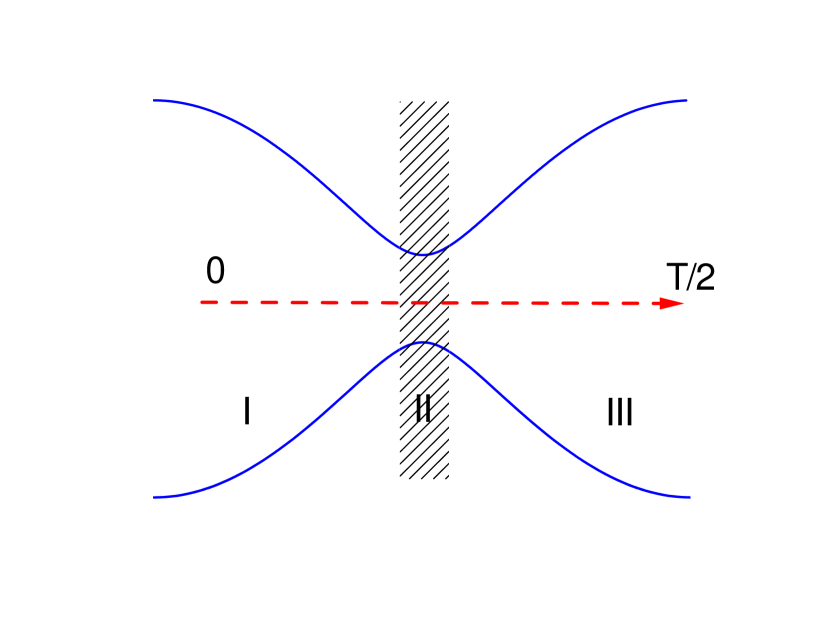
Figure 1: Schematic representation of the instantaneous energy levels of a two-level system during its evolution from $t=0$ to $t=T/2$ with $\epsilon(t)=5\cos t$ and $\Delta=0.5$. Regions I and III correspond to adiabatic evolution while region II (shaded area) denotes the impulse region. The width of the impulse region is taken to be close to zero in the adiabatic-impulse approximation. The red line indicates the evolution of the system for the first half-cycle from $t=0$ to $t=T/2$. The remaining half-cycle is traversed in the opposite direction so that each region is traversed twice during evolution from $t=0$ to $t=T$.

To chart out the computation of $U$ using this method, we first note that the instantaneous eigenvalue of $U(t,0)$ can be trivially found from Eq. (28) and are given by

$$E_{\pm}(t) = \pm E(t),\quad E(t)=\sqrt{\epsilon(t)^{2}+\Delta_{0}^{2}}.$$ (29)

The corresponding instantaneous eigenvectors are given by

$$|\psi_{-}(t)\rangle = (u(t),v(t))^{T},\,\,|\psi_{+}(t)\rangle=(-v(t),u(t))^{T},$$

$$u(t) = \frac{\Delta_{0}}{D(t)},\quad v(t)=(E(t)+\epsilon(t))/D(t),$$

$$D(t) = \sqrt{[E(t)+\epsilon(t)]^{2}+\Delta_{0}^{2}}.$$ (30)

A plot of this instantaneous energy gap $\delta E(t)=2E(t)$ is shown in Fig. 1. The plot clearly indicates that the evolution time may be divided into two distinct regimes. In the first regime, shown in Fig. 1 as regions I and III, one has $\delta E^{2}(t)/|\hbar\,d\delta E(t)/dt|\gg 1$; thus as per standard Landau criterion, the system in these regions undergo near-adiabatic evolution. In the other regime, denoted in Fig. 1 as region II, $\delta E^{2}(t)/|\hbar\,d\delta E(t)/dt|\leq 1$ and the evolution leads to the production of excitations. This is the impulse region. The key approximation of the adiabatic-impulse technique which enables one to analytically compute $U$ is to treat the impulse region as one with an infinitesimal width around a minimum of the instantaneous energy gap. Since this approximation clearly becomes better at lower drive frequencies, the adiabatic-impulse method naturally describes the low drive-frequency regime accurately.

To compute $U(t,0)$ we note that the wave function of the system at any time can be expressed in the adiabatic or the moving basis as

$$|\psi(t)\rangle = c_{1}(t)\left(\begin{array}[]{c}u(t)\\ v(t)\end{array}\right)+c_{2}(t)\left(\begin{array}[]{c}-v(t)\\ u(t)\end{array}\right),$$ (35)

where $c_{1}(0)=1$ and $c_{2}(0)=0$. The choice of this basis makes the computation simpler, specially in the adiabatic regions I and III. We note that the basis vectors

$$|\psi_{\rm ad}^{(0)}\rangle = (u(t),v(t))^{T},$$

$$|\psi_{\rm ad}^{(1)}\rangle = (-v(t),u(t))^{T},$$ (36)

are related to those in the diabatic basis (given by $|\psi_{\rm dia}^{(0)}\rangle=(u(t=0),v(t=0))^{T}$ and $|\psi_{\rm dia}^{(1)}\rangle=(-v(t=0),u(t=0))^{T}$) by the standard transformation

$$\left(\begin{array}[]{c}|\psi_{\rm ad}^{(0)}\rangle\\ |\psi_{\rm ad}^{(1)}\rangle\end{array}\right) = \Lambda(t)\left(\begin{array}[]{c}|\psi_{\rm dia}^{(0)}\rangle\\ |\psi_{\rm dia}^{(1)}\rangle\end{array}\right),$$ (41)

$$\Lambda(t) = \left(\begin{array}[]{cc}\eta&\sqrt{1-\eta^{2}}\\ -\sqrt{1-\eta^{2}}&\eta\end{array}\right),$$ (44)

$$\eta\equiv\eta(t) = u(t)u(0)+v(t)v(0).$$ (45)

We note that the adiabatic and the diabatic basis coincide at $t=0$ where $\eta=1$.

In region I, as discussed above, the system does not produce any excitations. Thus the dynamics leads to a kinetic phase. This can be seen most simply in the adiabatic basis where a straightforward calculation, charted out in Refs. rev4, , topo4, , and graphene1, shows

$$c_{1}(t) = \exp[-i\zeta(t,0)]c_{1}(0),$$

$$c_{2}(t) = \exp[i\zeta(t,0)]c_{2}(0),$$

$$\zeta(t_{1},t_{2}) = \frac{1}{\hbar}\int_{t_{2}}^{t_{1}}dt^{\prime}E(t^{\prime}).$$ (46)

Thus in this basis one can define $U^{\prime}_{I}(t,0)=\exp[-i\sigma_{z}\zeta(t,0)]$ which relates $(c_{1}(t),c_{2}(t))^{T}$ to their values at $t=0$,

$$\left(\begin{array}[]{c}c_{1}(t)\\ c_{2}(t)\end{array}\right) = U^{\prime}_{I}(t,0)\left(\begin{array}[]{c}c_{1}(0)\\ c_{2}(0)\end{array}\right).$$ (51)

Note that although $U^{\prime}_{I}(t,0)$ is not the true evolution operator, it acts as an useful operator which provide a handy calculational tool in the adiabatic basis. To find the true evolution operator $U_{I}(t,0)$ for all $t$ where the system is in region I, we use Eq. (45) to obtain

$$|\psi_{I}(t)\rangle = \Lambda(t)U^{\prime}_{I}(t,0)|\psi_{\rm in}\rangle=U_{I}(t,0)|\psi_{\rm in}\rangle,$$ (52)

where in the last line we have used the definition $|\psi_{I}(t)\rangle=U_{I}(t,0)|\psi_{\rm in}\rangle$. This finally yields

$$U_{I}(t) = \left(\begin{array}[]{cc}e^{-i\zeta(t,0)}\eta(t)&-e^{i\zeta(t,0)}\sqrt{1-\eta^{2}}\\ e^{-i\zeta(t,0)}\sqrt{1-\eta^{2}}&e^{i\zeta(t,0)}\eta(t)\end{array}\right),$$ (55)

which allows us to track the time evolution of the system in region I. A similar calculation holds for any adiabatic region.

Next, we consider region II which is reached at $t=t_{0}$ as shown in Fig. 1. Here the drive leads to the production of defects. The width of this region, $\Delta t$, is approximated to be infinitesimal within the adiabatic-impulse approximation. The width of region II can be computed from the Landau criteria $\delta E^{2}\leq\hbar|d\delta E/dt|$; since $|d\delta E/dt|\sim\omega_{D}$, it is clear that $\Delta t$ decreases with decreasing $\omega_{D}$. Thus this approximation becomes better with decreasing $\omega_{D}$. Typically one assumes that the width of this region is small enough so that the wave functions immediately before entering region II and immediately after leaving it are related by a transfer matrix ${\mathcal{N}}$

$$\left(\begin{array}[]{c}c_{1}(t_{0}+\Delta t)\\ c_{2}(t_{0}+\Delta t)\end{array}\right) = {\mathcal{N}}\left(\begin{array}[]{c}c_{1}(t_{0}-\Delta t)\\ c_{2}(t_{0}-\Delta t)\end{array}\right).$$ (60)

To compute ${\mathcal{N}}$, one typically uses a linearized description of $H$. Within this approximation one writes $H(t)\simeq[\epsilon(t_{0})+(t-t_{0})\dot{\epsilon}(t_{0})]\sigma_{z}+\sigma_{x}\Delta_{0}$, where $t_{0}$ is the time at which the system reaches region II. The linearization of $H(t)$ around $t=t_{0}$ reduces the problem to that of computing the probability of the generation of defects due to Kibble-Zureck mechanism rev7 . It is well-known that the probability $p$ of defect formation in this case is given by

$$p = \exp[-2\pi\delta],\quad\delta=\Delta_{0}^{2}/[2\hbar\dot{\epsilon}_{0}(t_{0})].$$ (61)

So for the two-level system, the probability for the system to remain in its starting state after crossing the impulse region is $1-p$. Thus the diagonal elements of ${\mathcal{N}}$ yields $N_{11},N_{22}\sim\sqrt{1-p}$ while its off-diagonal element satisfies $N_{12},N_{21}\sim\sqrt{p}$. The detailed computation of ${\mathcal{N}}$ from these considerations has been charted out in Refs. rev4, , graphene1, , child1, and kaya1, and yields

$${\mathcal{N}} = \left(\begin{array}[]{cc}\sqrt{1-p}e^{-i\phi_{0}}&-\sqrt{p}\\ \sqrt{p}&\sqrt{1-p}e^{i\phi_{0}}\end{array}\right),$$ (64)

$$\phi_{0} = \phi_{\rm st}-\pi,$$ (65)

$$\phi_{\rm st} = \frac{\pi}{4}+\delta\ln\delta+{\rm Arg}\Gamma[1-i\delta],$$

where $\phi_{\rm st}$ is the Stoke’s phase and $\Gamma$ denotes the gamma function.

At the end of region II, one can write

$$\left(\begin{array}[]{c}c_{1}(t_{0}+\Delta t)\\ c_{2}(t_{0}+\Delta t)\end{array}\right) = {\mathcal{N}}U^{\prime}_{I}(t_{0}-\Delta t,0)\left(\begin{array}[]{c}1\\ 0\end{array}\right).$$ (70)

Thus the evolution operator after the system has traversed region II is given by

$$U_{II}(t_{0}+\Delta t,0) = \Lambda(t_{0}+\Delta t){\mathcal{N}}U^{\prime}_{I}(t_{0}-\Delta t,0).$$ (71)

This procedure can be continued to obtain $U(t,0)$ for all $t\leq T$. To this end, we note that the system crosses the impulse region twice, at $t=t_{0}$ and $t=T-t_{0}$; the rest of the dynamics consists of passing through adiabatic regions. The evolution operator during any time $t$ can be written as

$$U(t,0) = \Lambda(t)\,U^{\prime}_{I}(t,0),\quad t\leq t_{0}$$

$$= \Lambda(t)\,U^{\prime}_{I}(t,t_{0})\,{\mathcal{N}}\,U^{\prime}_{I}(t_{0},0),\quad T-t_{0}\leq t\leq t_{0}$$

$$= \Lambda(t)\,U^{\prime}_{I}(t,T-t_{0})\,{\mathcal{N}}^{T}\,U^{\prime}_{I}(T-t_{0},t_{0})$$

$$\times~{}{\mathcal{N}}\,U^{\prime}_{I}(t_{0},0),\quad T\leq t\leq T_{0}-t.$$

where ${\mathcal{N}}^{T}$ denotes the transpose of ${\mathcal{N}}$. Thus this method may be used to compute $U(t,0)$ for all $t\leq T$ and thus obtain information about the micromotion.

The instantaneous eigenvalues $\lambda_{\pm}(t)=\exp[\pm i\theta(t)]$ of the evolution operator $U(t,0)$ are called phase bands. They play an important role in charting out possible topological transitions in driven many-body systems topo1 ; topo5 . Moreover, at $t=T$, one can read off the eigenvalues of the Floquet Hamiltonian from them: $\lambda_{\pm}(T)=\exp[\pm i\epsilon_{F}T/\hbar]$. A straightforward computation, charted out in Refs. rev4, and graphene1, yields

$$\cos\theta(t) = \eta\cos\alpha_{1}(t),\quad t\leq t_{0}$$

$$= \eta\sqrt{1-p}\cos\alpha_{2}(t)+\sqrt{p(1-\eta^{2})}\cos\beta_{2}(t),\quad t_{0}\leq t\leq T-t_{0}$$

$$= \eta[p\cos\alpha_{3}(t)+(1-p)\cos\beta_{3}(t)]+\sqrt{p(1-p)(1-\eta^{2})}[\cos(\alpha_{3}-\phi_{\rm st})-\cos(\beta_{3}-\phi_{\rm st})],\quad t\geq T_{0}-t$$

where we have diagonalized $U(t,0)$ in Eq. (III) to obtain these expressions, and $\alpha_{1,2,3}$ and $\beta_{2,3}$ are given by

$$\alpha_{1}(t) = \zeta(t,0),\quad\alpha_{2}(t)=\zeta(t,0)+\phi_{\rm st},$$

$$\beta_{2}(t) = \zeta(t,t_{0})-\zeta(t_{0},0),\quad\alpha_{3}(t)=2\phi_{\rm st}+\zeta(t,0),$$

$$\beta_{3}(t) = \zeta(t_{0},0)-\zeta(T-t_{0},t_{0})+\zeta(t,T-t_{0}).$$ (74)

The computational scheme charted above brings out two aspects of the method. First, it can be directly applied to a class of integrable spin models which can be written in terms of free fermions via a Jordan-Wigner transformation. These models include the one-dimensional Ising and XY models and the two-dimensional Kitaev models isingref ; kitaevref . In addition, it can also be used to describe the dynamics of Dirac quasiparticles in graphene or atop a topological insulator surface grapheneref ; tiref , and Weyl fermions in 3D band systems weylref . All these systems can be represented by fermionic Hamiltonians of the form

$$H = \sum_{\vec{k}}\psi_{\vec{k}}^{\dagger}H_{\vec{k}}\psi_{\vec{k}},$$ (75)

where $H_{\vec{k}}$ is given by Eq. (28) with $\epsilon_{0}(t)\to\epsilon_{\vec{k}}(t)$ and $\Delta_{0}\to\Delta_{\vec{k}}$. The precise forms of $\epsilon_{\vec{k}}(t)$ and $\Delta_{\vec{k}}$ depend on the model and are well-known isingref ; kitaevref ; grapheneref ; tiref ; weylref . Second, the method provides an easy access to the micromotion in these systems; thus it allows one to address the phase bands of these models. It has been recently pointed out that the understanding of topological transitions in such driven systems requires an analysis of their phase bands $\theta(\vec{k},t)$, and a knowledge of only their Floquet spectrum $\epsilon_{F}(\vec{k})=\theta(\vec{k},T)/T$ may not be sufficient topo5 . We note in passing that this scheme can be generalized to cases where both $\epsilon$ and $\Delta$ are time dependent; the details of such generalizations have been charted out in Refs. graphene1, and sau1, .

In what follows, we will provide an example of graphene in the presence of external radiation where one can use this method to detect a topological transition at $t=T/3$ graphene1 . The Hamiltonian of graphene in the presence of an external radiation is given by Eq. (75) with $\epsilon_{\vec{k}}(t)=-{\rm Re}Z_{\vec{k}}(t)$ and $\Delta_{\vec{k}}(t)={\rm Im}Z_{\vec{k}}(t)$, where

$$Z_{\vec{k}}(t) = -\sum_{p=\pm 1}e^{i(\cos(\omega t-p\pi/3)+(k_{x}+\sqrt{3}pk_{y})/2)}$$ (76)

$$-~{}e^{i(\cos(\omega t)-k_{x})},$$

where $\alpha=eA_{0}/c$, and $A_{0}$ and $\omega$ are the amplitude and frequency of the circularly polarized external radiation represented by the vector potential $\vec{A}=A_{0}(\cos(\omega t),\sin(\omega t))$. It can be directly checked that at the $\Gamma$ point of the Brillouin zone ($(k_{x},k_{y})=(0,0)$), $H_{\vec{k}}$ satisfies

$$H_{\vec{k}}(t) = H_{\vec{k}}(T-t),$$ (77)

$$H_{\vec{k}}(T/3\pm t) = H_{\vec{k}}(t)=H_{\vec{k}}(2T/3\pm t),$$

$$U(2T/3,0) = [U(T/3,0)]^{2},\quad U(T,0)=[U(T/3,0)]^{3},$$

where $U$ represents the evolution operator at the $\Gamma$ point. This shows that a phase band crossing leading to a change of topology of the driven system at $t=T/3$ (which amounts to $U(T/3,0)=\pm I$) necessarily shows analogous crossing at $t=T$; however, the reverse is not true.

The verification of such crossings at $t=T/3$ and $2T/3$ has been carried out in detail in Ref. graphene1, . A somewhat lengthy calculation yields an analytical expression for the phase bands within the adiabatic-impulse approximation. In terms of the probability $p_{\Gamma}$ for the formation of excitations formation probability and the associated Stuckelberg phase $\Phi_{\Gamma}$, one finds that the expression for the phase band $\phi_{\Gamma}$ at the $\Gamma$ point is graphene1

$$\cos(\phi(T/3)) = p_{\Gamma}+(1-p_{\Gamma})\cos(2\Lambda_{\Gamma}),$$ (78)

$$\Lambda_{\Gamma} = \Phi_{\Gamma}+2\int_{0}^{T/6}dt\sqrt{\epsilon_{\vec{k}=0}^{2}(t)+\Delta_{\vec{k}=0}^{2}(t)}.$$

It was shown that the band crossings that lead to a change in topology of the state of the driven system at $t=T/3$ requires $\cos[\phi_{\Gamma}(T/3)]=+(-)1$ for crossings through the zone center (edge). The crossings through the zone center thus requires $\Lambda_{\Gamma}=m\pi$ for $m\in Z$. The crossing through the zone edge, in contrast, necessitates $\cos[2\Lambda_{\Gamma}]=-(1+p_{\Gamma})/(1-p_{\Gamma})$; this is clearly untenable for real $\Lambda$ and hence the adiabatic-impulse approximation predicts that all such band crossings at $t=T/3$ should occur through the zone center. This fact has been numerically verified in Ref. graphene1, . A similar analysis has been carried out for other values of $T$ and at other points in the graphene Brillouin zone. In all cases, the prediction of the adiabatic-impulse method provides a near-exact match with exact numerics as long as the drive frequency is small compared to the nearest-neighbor hopping amplitude of the electrons in graphene; in addition it provides analytical conditions for phase band crossings which help in obtaining a semi-analytic understanding of the phase diagram of periodically driven graphene graphene1 . Moreover, such an analysis can be easily extended to a wide class of driven spin and fermionic systems which host Dirac-like quasiparticles. It thus provides a complete picture of the low-frequency behavior of a wide range of integrable models.

IV Floquet perturbation theory

In this section, we discuss a perturbative method to find the Floquet Hamiltonian $H_{F}$ or periodically driven many-body Hamiltonians of the form $H(t)=H_{0}(t)+gV(t)$, where $H_{0}(t)(V(t))=H_{0}(t+T)(V(t+T))$ (note that $H_{0}(t)$ or $V(t)$ may be time-independent), $g\ll 1$, and crucially, $H_{0}(t)$ consists of mutually commuting terms. We call this Floquet perturbation theory (FPT) whereby $H_{F}$ is obtained as a power series in $g$ soori10 ; flscar1 ; haldar19 . This method is particularly suited to address the nature of the Floquet Hamiltonian at intermediate and low drive frequencies, unlike the high-frequency FM expansion.

As the first example, suppose that the Hamiltonian $H$ can be written as a sum of two parts, $H(t)$ which varies periodically in time with a period $T=2\pi/\omega_{D}$, and a perturbation $V$ which is time-independent. Thus $H(t)=H_{0}(t)+V$. Since $H_{0}(t)$ commutes with itself at different times, we can work in the basis of eigenstates of $H_{0}(t)$ which are time-independent and orthonormal. We denote these as $|n\rangle$, so that $H_{0}(t)|n\rangle=E_{n}(t)|n\rangle$, and $\langle m|n\rangle=\delta_{mn}$.

We now find solutions of the time-dependent Schrödinger equation

$$i\hbar\frac{\partial\psi_{n}}{\partial t}~{}=~{}H(t)\psi_{n}(t)$$ (79)

which satisfy the Floquet eigenstate condition

$$\psi_{n}(T)~{}=~{}e^{i\theta_{n}}~{}\psi_{n}(0),$$ (80)

where $e^{i\theta_{n}}$ is the Floquet eigenvalue.

For $V=0$, we have

$$\psi_{n}(t)~{}=~{}e^{-(i/\hbar)\int_{0}^{t}dt^{\prime}E_{n}(t^{\prime})}~{}|n\rangle,$$ (81)

so that the eigenvalue of the Floquet unitary

$$U~{}=~{}{\cal T}~{}e^{-(i/\hbar)\int_{0}^{T}dtH(t)}$$ (82)

is given by

$$e^{i\theta_{n}}~{}=~{}e^{-(i/\hbar)\int_{0}^{T}dtE_{n}(t)}.$$ (83)

For $V$ non-zero but small, we will develop a FPT to first order in $V$. We first consider non-degenerate perturbation theory; the meaning of non-degenerate will become clear below. We assume that the $n$-th eigenstate can be written as

$$\psi_{n}(t)~{}=~{}\sum_{m}~{}c_{m}(t)~{}e^{-(i/\hbar)\int_{0}^{t}dt^{\prime}E_{m}(t^{\prime})}~{}|m\rangle,$$ (84)

where $c_{n}(t)=1~{}+$ terms of order $V$ for all $t$, while $c_{m}(t)$ is of order $V$ for all $m\neq n$ and all $t$. Eq. (79) then implies

$$i\hbar~{}\sum_{m}\dot{c}_{m}(t)e^{-(i/\hbar)\int_{0}^{t}dt^{\prime}E_{m}(t^{\prime})}~{}|m\rangle$$ (85)

$$= V~{}\sum_{m}~{}c_{m}(t)~{}e^{-(i/\hbar)\int_{0}^{t}dt^{\prime}E_{m}(t^{\prime})}~{}|m\rangle,$$

where $\dot{c}_{m}$ denotes $dc_{m}/dt$. Taking the inner product of Eq. (85) with $\langle n|$, we find, to first order in $V$, that $i\hbar\dot{c}_{n}=\langle n|V|n\rangle$. Choosing $c_{n}(0)=1$, we then have

$$c_{n}(t)~{}=~{}e^{-(i/\hbar)\langle n|V|n\rangle t}.$$ (86)

This gives

$$\psi_{n}(t) = e^{-(i/\hbar)(\langle n|V|n\rangle t~{}+~{}\int_{0}^{t}dt^{\prime}E_{n}(t^{\prime}))}~{}|n\rangle$$ (87)

$$+~{}\sum_{m\neq n}~{}c_{m}(t)~{}e^{-(i/\hbar)\int_{0}^{t}dt^{\prime}E_{m}(t^{\prime})}~{}|m\rangle.$$

Next, taking the inner product of Eq. (85) with $\langle m|$, where $m\neq n$, we find, to first order in $V$, that

$$\dot{c}_{m}~{}=~{}-~{}\frac{i}{\hbar}~{}\langle m|V|n\rangle~{}e^{(i/\hbar)\int_{0}^{t}dt^{\prime}[E_{m}(t^{\prime})-E_{n}(t^{\prime})]}.$$ (88)

(We have ignored a factor of $e^{(i/\hbar)\langle n|V|n\rangle t}$ on the right hand side of Eq. (88) since we are only interested in terms of first order in $V$). Integrating Eq. (88) gives

$$c_{m}(T)~{}=~{}c_{m}(0)~{}-~{}\frac{i}{\hbar}~{}\langle m|V|n\rangle~{}\int_{0}^{T}dt~{}e^{i\int_{0}^{t}dt^{\prime}[E_{m}(t^{\prime})-E_{n}(t^{\prime})]}.$$ (89)

Since we know that Eq. (87) satisfies

$$\psi_{n}(T)~{}=~{}e^{-(i/\hbar)(\langle m|V|n\rangle T~{}+~{}\int_{0}^{T}dtE_{n}(t))}~{}\psi_{n}(0),$$ (90)

we must have, to first order in $V$,

$$c_{m}(T)~{}=~{}e^{(i/\hbar)\int_{0}^{T}dt[E_{m}(t)-E_{n}(t)]}~{}c_{m}(0)$$ (91)

for all $m\neq n$. This, along with Eq. (89), means that we must choose

$$c_{m}(0)~{}=~{}-\frac{i}{\hbar}~{}\langle m|V|n\rangle~{}\frac{\int_{0}^{T}dt~{}e^{(i/\hbar)\int_{0}^{t}dt^{\prime}[E_{m}(t^{\prime})-E_{n}(t^{\prime})]}}{e^{(i/\hbar)\int_{0}^{T}dt[E_{m}(t)-E_{n}(t)]}~{}-~{}1}.$$ (92)

We see that $c_{m}(t)$ is indeed of order $V$ provided that the denominator on the right hand side of Eq. (92) does not vanish; we call this case non-degenerate. If

$$e^{(i/\hbar)\int_{0}^{T}dt[E_{m}(t)-E_{n}(t)]}~{}=~{}1,$$ (93)

we have a resonance between states $|m\rangle$ and $|n\rangle$, and the above analysis breaks down. We then have to develop a degenerate FPT as discussed below.

If there are several states which are connected to $|n\rangle$ by the perturbation $V$, Eq. (92) describes the amplitude to go to each of them from $|n\rangle$. Up to order $V^{2}$, the total probability of excitation away from $|n\rangle$ is given by $\sum_{m\neq n}|c_{m}(0)|^{2}$. If $c_{m}(0)$ turns out to be zero for all $m\neq n$ (this can happen if either the matrix element $\langle m|V|n\rangle=0$ or the numerator of the expression in Eq. (92) vanishes), the Floquet eigenstate remains equal to $\psi_{n}$ up to first order in $V$. This is an example of dynamical freezing.

Next we consider degenerate perturbation theory. Suppose that there are $p$ states $|m\rangle$ ($m=1,2,\cdots,p$) which have energies $E_{m}$ and satisfy Eq. (93) for every pair of states $(m,n)$ lying in the range 1 to $p$. Ignoring all the other states for the moment, we assume that a solution of the Schrödinger equation is given by

$$\psi_{n}(t)~{}=~{}\sum_{m=1}^{p}~{}c_{m}(t)~{}e^{-(i/\hbar)\int_{0}^{t}dt^{\prime}E_{m}(t^{\prime})}~{}|m\rangle,$$ (94)

where we now allow all the $c_{m}(t)$’s to be of order 1. To first order in $V$, we can then replace $c_{m}(t)$ by the time-independent constants $c_{m}(0)$ on the right hand side of Eq. (85). Upon integrating from $t=0$ to $T$, we obtain

$$c_{m}(T) = c_{m}(0)~{}-~{}\frac{i}{\hbar}~{}\sum_{n=1}^{p}~{}\langle m|V|n\rangle$$ (95)

$$\times\int_{0}^{T}dt~{}e^{(i/\hbar)\int_{0}^{t}dt^{\prime}[E_{m}(t^{\prime})-E_{n}(t^{\prime})]}~{}c_{n}(0).$$

This can be written as a matrix equation

$$c(T)~{}=~{}[I~{}-~{}\frac{iH^{\prime}T}{\hbar}]~{}c(0),$$ (96)

where $c(t)$ denotes the column $(c_{1}(t),c_{2}(t),\cdots,c_{p}(t))^{T}$ (where the superscript $T$ denotes transpose), $I$ is the $p$-dimensional identity matrix, and $H^{\prime}$ is a $p$-dimensional Hermitian matrix with matrix elements

$$(H^{\prime})_{mn}~{}=~{}\frac{\langle m|V|n\rangle}{T}~{}\int_{0}^{T}dte^{(i/\hbar)\int_{0}^{t}dt^{\prime}[E_{m}(t^{\prime})-E_{n}(t^{\prime})]}.$$ (97)

Let the eigenvalues of $H^{\prime}$ be $\epsilon_{n}$ ($n=1,2,\cdots,p$). To first order in $V$, $I-iH^{\prime}T/\hbar$ is a unitary matrix and therefore has eigenvalues of the form $e^{-i\epsilon_{n}T/\hbar}$; the corresponding eigenstates satisfy

$$c(T)~{}=~{}e^{-i\epsilon_{n}T/\hbar}~{}c(0).$$ (98)

Next, we want the wave function in Eq. (94) to satisfy Eq. (80). This implies that the Floquet eigenvalues are related to the eigenvalues of $H^{\prime}$ as

$$e^{i\theta_{n}}~{}=~{}e^{-(i/\hbar)(\epsilon_{n}T~{}+~{}\int_{0}^{T}dtE_{n}(t))},$$ (99)

where we have used the resonance condition that $e^{-(i/\hbar)\int_{0}^{T}dtE_{n}(t)}$ has the same value for all $n=1,2,\cdots,p$.

Given a Floquet unitary $U(T)$, we can define a Floquet Hamiltonian $H_{F}$ using Eq. (1). Comparing this with Eqs. (96) and (97), we see that the matrix elements of $H_{F}$ are

$$(H_{F})_{mn} = \frac{\langle m|V|n\rangle}{T}\int_{0}^{T}dte^{(i/\hbar)\int_{0}^{t}dt^{\prime}[E_{m}(t^{\prime})-E_{n}(t^{\prime})]}$$ (100)

$$+~{}\Bigl{(}\frac{1}{T}\int_{0}^{T}dt~{}E_{n}(t)\Bigr{)}~{}\delta_{mn},$$

where we have assumed that $\int_{0}^{T}dt~{}E_{n}(t)$ has the same value for all $n$. [This is a special case of Eq. (93). More generally, Eq. (93) allows the values of $\int_{0}^{T}dt~{}E_{n}(t)$ to differ from each other by non-zero integer multiples of $2\pi\hbar$, but we will not consider that possibility here].

Unlike the FM expansion rev1 ; mikami16 , FPT does not assume the drive frequency $\omega_{D}$ to be large compared to the other parameters of the system. It only assumes the amplitude of the driving to be large. This will become clear in the examples discussed below where we will see that the Floquet Hamiltonian is effectively an expansion in the inverse of the driving amplitude.

As the first application of the above formalism, we consider a simple model with a single spin-1/2 which is governed by a Hamiltonian $H(t)=H_{0}(t)+V$, where udupa20

$$H_{0} = \lambda\cos(\omega t)~{}\sigma^{x},$$

$$V = g_{1}~{}\sigma^{x}~{}+~{}g_{2}~{}\sigma^{y},$$ (101)

and we will assume that $\lambda\gg g_{1},~{}g_{2}$. The unperturbed problem given by $i\hbar\partial\psi/\partial t=H_{0}\psi$ has solutions

$$\psi_{1}(t) = e^{-i(\lambda/\hbar\omega)\sin(\omega t)}~{}|1\rangle,$$

$$\psi_{2}(t) = e^{i(\lambda/\hbar\omega)\sin(\omega t)}~{}|2\rangle,$$

$${\rm where}~{}~{}|1\rangle = \frac{1}{\sqrt{2}}\begin{pmatrix}1\\ 1\end{pmatrix}~{}~{}{\rm and}~{}~{}|2\rangle~{}=~{}\frac{1}{\sqrt{2}}\begin{pmatrix}1\\ -1\end{pmatrix},$$ (102)

and the corresponding eigenvalues of $H_{0}(t)$ are $E_{1}(t)=\lambda\cos(\omega t)$ and $E_{2}(t)=-\lambda\cos(\omega t)$ respectively. Since these satisfy Eq. (93) we have to use degenerate perturbation theory. Following Eqs. (94-100), and using the identity abramowitz

$$\int_{0}^{T}dt~{}e^{(i/\hbar)\int_{0}^{t}dt^{\prime}2\lambda\cos(\omega t^{\prime})}~{}=~{}TJ_{0}\Big{(}{\frac{2\lambda}{\hbar\omega}}\Big{)},$$ (103)

we find that the Floquet Hamiltonian is

$$H_{F}~{}=~{}g_{1}~{}\sigma^{x}~{}+~{}g_{2}~{}J_{0}\Big{(}{\frac{2\lambda}{\hbar\omega}}\Big{)}~{}\sigma^{y}.$$ (104)

The Bessel function $J_{0}(z)\to 1$ when $z\to 0$ and goes as $\sqrt{2/(\pi z)}\cos(z-\pi/4)$ when $z\to\infty$. It is clear that Eqs. (101) and (104) are consistent with each other in the limit $\lambda/(\hbar\omega)\to 0$; in particular, $H_{F}$ approaches the time-averaged value $(1/T)\int_{0}^{T}dtH(t)$ in the high-frequency limit. The limit $\lambda/(\hbar\omega)\to\infty$ is less trivial; we then see that the driving-dependent term in $H_{F}$ goes to zero as $\sqrt{\hbar\omega/\lambda}$ apart from an oscillatory factor. Incidentally, we note that if we shift the time, i.e., change $\cos(\omega t)\to\cos(\omega(t+t_{0}))$ in Eq. (101), the expression for the Floquet Hamiltonian in Eq. (104) would change.

Note that if we had considered a different limit where $\hbar\omega\gg\lambda,g$, and used the FM expansion, we would have obtained an expansion in powers of $\lambda/(\hbar\omega)$ and $g/(\hbar\omega)$. A resummation of all the terms which are of first order in $g$ would then give back the expression in Eq. (104). Thus first-order FPT gives an expression for $H_{F}$ which is a resummation of all the terms in the FM expansion which are of first order in the perturbation $V$.

Next, we apply FPT to a periodically driven spin chain called the PXP model flscar1 . We consider $H(t)=H_{0}(t)+V$, where

$$H_{0}(t) = \frac{\lambda(t)}{2}~{}\sum_{l}~{}\sigma^{z}_{l},$$

$$V = g~{}\sum_{l}~{}P_{l-1}\sigma_{l}^{x}P_{l+1},$$ (105)

where $P_{l}=(1-\sigma_{l}^{z})/2$ is the projection operator to the spin-down state at site $l$. The presence of the projection operator in the second line of Eq. (105) makes the Hamiltonian $V$ non-integrable. We will consider a driving with the form of a square pulse,

$$\lambda(t) = -~{}\lambda~{}~{}~{}{\rm for}~{}~{}~{}0~{}<~{}t~{}<~{}T/2$$ (106)

$$= +~{}\lambda~{}~{}~{}{\rm for}~{}~{}~{}T/2~{}<~{}t~{}<~{}T,$$

and $\lambda(t+T)=\lambda(t)$ for all times.

We now apply FPT assuming that $\lambda\gg g$. We choose the $\sigma_{l}^{z}$ basis for the states. According to the unperturbed Hamiltonian $H_{0}$ in Eq. (105), we see that such states $|n\rangle$ have an instantaneous energy eigenvalue $E_{n}(t)=(\lambda(t)/2)~{}\sum_{l}~{}\sigma^{z}_{l}$. We now consider the effect to first order of the perturbation $V$ in Eq. (105). If $|m\rangle$ and $|n\rangle$ are two states which are connected by $V$, they differ by the value of $\sigma_{l}^{z}$ at only one site and therefore $E_{m}(t)-E_{n}(t)=\lambda(t)$. Hence Eq. (93) is satisfied and we have to use degenerate perturbation theory. The integral in Eq. (95) is found to be

$$\int_{0}^{T}dt~{}e^{(i/\hbar)\int_{0}^{t}dt^{\prime}[E_{m}(t^{\prime})-E_{n}(t^{\prime})]}~{}=~{}\frac{i2\hbar}{\lambda}~{}(e^{-i\lambda T/(2\hbar)}~{}-~{}1).$$ (107)

We see that if $e^{-i\lambda T/(2\hbar)}=1$, i.e., if

$$\frac{\lambda}{\hbar\omega}~{}=~{}2p,$$ (108)

where $p$ is an integer, then the expression in Eq. (107) vanishes. This means that even in degenerate perturbation theory, there is no change in the Floquet eigenvalues and they remain equal to 1.

We can now use Eqs. (100) and (107) to derive the Floquet Hamiltonian. If $|m\rangle$ and $|n\rangle$ are two states which are connected by the perturbation $V$, we have $\langle m|V|n\rangle=g$ (note that $|m\rangle$ and $|n\rangle$ must necessarily be different from each other). We then obtain

$$(H_{F})_{mn} = \frac{i2g\hbar}{\lambda T}~{}(e^{-i\lambda T/(2\hbar)}~{}-~{}1)$$ (109)

$$= \frac{2g\hbar\omega}{\pi\lambda}~{}e^{-i\pi\lambda/(2\hbar\omega)}~{}\sin\Bigl{(}\frac{\pi\lambda}{2\hbar\omega}\Bigl{)}.$$

We thus see that

$$H_{F}~{}=~{}g~{}\frac{\sin\gamma}{\gamma}~{}\sum_{l}~{}P_{l-1}[\cos\gamma~{}\sigma_{l}^{x}~{}+~{}\sin\gamma~{}\sigma_{l}^{y}]P_{l+1},$$ (110)

where $\gamma=\pi\lambda/(2\hbar\omega)$. We now see that if Eq. (108) holds, the Floquet Hamiltonian vanishes to first order in $g/\lambda$. We then have to go to higher orders or study the model numerically to understand its behavior flscar1 .

Eq. (110) shows that in the limit $\lambda\to\infty$, $H_{F}$ goes to zero as $1/\lambda$ apart from some oscillatory factors. The different power laws, $1/\sqrt{\lambda}$ versus $1/\lambda$, in Eqs. (104) and (110) are related to the fact that the driving term has different forms in the two cases, $\lambda\cos(\omega t)$ in the first case and the square pulse in Eq. (106) in the second case.

Finally, we consider a case where the Floquet Hamiltonian $H_{F}$ has no contributions to first order in the perturbation and we have to go up to second order. Further, we will take the periodically driven part of the Hamiltonian to be much smaller than the time-independent part, and we will calculate $H_{F}$ only within a particular sector of eigenstates of the time-independent part. We consider a system with $M$ states $|\alpha\rangle$ in sector 1, all of which have energy $E_{1}$, and $N$ states $|\beta\rangle$ in sector 2, all of which have energy $E_{2}$. We introduce a small time-dependent coupling between states in the two sectors given by $V(t)$ and its Hermitian conjugate $V^{\dagger}(t)$ as follows, where $V(t+T)=V(t)$. Denoting states in sectors 1 and 2 by $\Psi_{1}$ and $\Psi_{2}$, which are columns with $M$ and $N$ entries respectively, the Schrödinger equation takes the form

$$i\hbar\frac{\partial\Psi_{1}}{\partial t} = E_{1}~{}\Psi_{1}~{}+~{}V~{}\Psi_{2},$$

$$i\hbar\frac{\partial\Psi_{2}}{\partial t} = E_{2}~{}\Psi_{2}~{}+~{}V^{\dagger}~{}\Psi_{1},$$ (111)

where $V$ is a $M\times N$ dimensional matrix. We now look for a Floquet eigenstate $\psi(t)$ which lies mainly in sector 1, namely,

$$\psi(t) = \left(\sum_{\alpha}c_{\alpha}(t)|\alpha\rangle\right)e^{-iE_{1}t/\hbar}$$ (112)

$$+~{}\left(\sum_{\beta}c_{\beta}(t)|\beta\rangle\right)e^{-iE_{2}t/\hbar},$$

where $c_{\alpha}(t)$ are of order 1 while $c_{\beta}(t)$ are of order $V$. Within sector 1, $H_{F}$ will be equal to $E_{1}$ plus terms of order $V^{2}$ (there are no contributions to first order in $V$ since the driving term has no matrix elements within sector 1). To calculate $H_{F}$, we proceed as follows. Denoting the column of coefficients $c_{\alpha}$ and $c_{\beta}$ collectively as $c_{1}$ and $c_{2}$ respectively, we have

$$i\hbar{\dot{c}}_{1} = e^{i(E_{1}-E_{2})t/\hbar}~{}V~{}c_{2},$$

$$i\hbar{\dot{c}}_{2} = e^{i(E_{2}-E_{1})t/\hbar}V^{\dagger}~{}c_{1}.$$ (113)

In the second equation in Eq. (113), we set $c_{1}(t)=c_{1}(0)$ on the right hand side since we want to find $c_{2}(t)$ only to order $V$. Integrating in time, we obtain

$$c_{2}(t)~{}-~{}c_{2}(0)~{}=~{}-\frac{i}{\hbar}~{}\int_{0}^{t}dt^{\prime}e^{i(E_{2}-E_{1})t^{\prime}/\hbar}V^{\dagger}(t^{\prime})c_{1}(0).$$ (114)

Since the Floquet eigenvalue in sector 1 is $e^{-iE_{1}t/\hbar}$ to first order in $V$, we require

$$c_{1}(T)~{}=~{}c_{1}(0)~{}~{}~{}{\rm and}~{}~{}~{}c_{2}(T)~{}=~{}e^{i(E_{2}-E_{1})t/\hbar}c_{2}(0)$$ (115)

to first order. Using this, we find from Eq. (114) that

$$c_{2}(t) = -\frac{i}{\hbar}~{}[\frac{\int_{0}^{T}dt^{\prime}e^{i(E_{2}-E_{1})t^{\prime}/\hbar}V^{\dagger}(t^{\prime})}{e^{i(E_{2}-E_{1})T/\hbar}-1}$$ (116)

$$~{}~{}~{}~{}~{}~{}+\int_{0}^{t}dt^{\prime}e^{i(E_{2}-E_{1})t^{\prime}/\hbar}V^{\dagger}(t^{\prime})]c_{1}(0).$$

The first equation in Eq. (113), then gives

$$c_{1}(T)~{}=~{}c_{1}(0)~{}-~{}\frac{i}{\hbar}\int_{0}^{T}dt~{}e^{i(E_{1}-E_{2})t/\hbar}V(t)c_{2}(t).$$ (117)

Since the Floquet Hamiltonian in sector 1 satisfies $\psi_{1}(T)=e^{-iH_{F}T/\hbar}\psi_{1}(0)$, we see from Eq. (117) that

$$H_{F} = E_{1}I~{}-~{}\frac{i}{\hbar T}\int_{0}^{T}dt~{}e^{i(E_{1}-E_{2})t/\hbar}~{}V(t)$$ (118)

$$\times~{}[\frac{\int_{0}^{T}dt^{\prime}e^{i(E_{2}-E_{1})t^{\prime}/\hbar}~{}V^{\dagger}(t^{\prime})}{e^{i(E_{2}-E_{1})T/\hbar}-1}$$

$$~{}~{}~{}~{}+~{}\int_{0}^{t}dt^{\prime}~{}^{i(E_{2}-E_{1})t^{\prime}/\hbar}~{}V^{\dagger}(t^{\prime})].$$

Next, the time periodicity of $V$ allows us to write it as

$$V~{}=~{}\sum_{n=-\infty}^{\infty}~{}V_{n}e^{-in\omega t}.$$ (119)

Eq. (118) then gives

$$H_{F}~{}=~{}E_{1}I~{}-~{}\sum_{n=-\infty}^{\infty}\frac{V_{n}V_{n}^{\dagger}}{E_{2}-E_{1}+n\hbar\omega}.$$ (120)

Eq. (120) shows that resonances occur whenever $(E_{2}-E_{1})/(\hbar\omega)$ is equal to an integer. However, near these points the above derivation of $H_{F}$ breaks down since the Floquet eigenstates will no longer have $c_{2}(t)$ much smaller than $c_{1}(t)$, which was an assumption made in order to calculate $H_{F}$. We note in passing that under a time shift $t\to t+t_{0}$, we would have $V_{n}\to V_{n}e^{-in\omega t_{0}}$ in Eq. (119), but the Floquet Hamiltonian in Eq. (120) would not change.

As an example of the above formalism, we consider the Hubbard model with two sites, labeled 1 and 2, where the hopping amplitude between the two sites, $g$, is much smaller than the on-site interaction strength $U$. itin15 We will take the phase of the hopping to be a sinusoidal function of time; this describes the effect of a periodically varying electric field through the Peierls prescription (see Sec. V.1). The Hamiltonian is

$$H = U~{}\sum_{n=1,2}~{}c_{n\uparrow}^{\dagger}c_{n\uparrow}c_{n\downarrow}^{\dagger}c_{n\downarrow}$$ (121)

$$-~{}g~{}\sum_{\sigma=\uparrow,\downarrow}~{}(e^{\frac{ia}{\omega}\sin(\omega t)}c_{1\sigma}^{\dagger}c_{2\sigma}$$

$$~{}~{}~{}~{}~{}~{}~{}~{}~{}~{}~{}~{}~{}~{}~{}+~{}e^{-\frac{ia}{\omega}\sin(\omega t)}c_{2\sigma}^{\dagger}c_{1\sigma}).$$

We will consider a half-filled system with two electrons. In the undriven system ($a=0$), we know that the low-energy states are described by an effective spin Hamiltonian given by $(4g^{2}/U)({\vec{S}}_{1}\cdot{\vec{S}}_{2}/\hbar^{2}-1/4)$. We will study what effect the driving has on the effective Hamiltonian which will now be denoted by $H_{F}$.

In the space of two-electron states, the states

$$|1\uparrow,2\uparrow\rangle~{}=~{}c_{1\uparrow}^{\dagger}c_{2\uparrow}^{\dagger}|0\rangle~{}~{}~{}{\rm and}~{}~{}~{}|1\downarrow,2\downarrow\rangle=c_{1\downarrow}^{\dagger}c_{2\downarrow}^{\dagger}|0\rangle$$ (122)

have a trivial dynamics since $H$ annihilates these states. Hence they are both Floquet eigenstates with Floquet eigenvalue equal to 1. Next, we study the states in which there is one spin-up electron and one spin-down electron. There are four such states,

$$|1\rangle = |1\uparrow,2\downarrow\rangle=c_{1\uparrow}^{\dagger}c_{2\downarrow}^{\dagger}|0\rangle,$$

$$|2\rangle = |1\downarrow,2\uparrow\rangle=c_{1\downarrow}^{\dagger}c_{2\uparrow}^{\dagger}|0\rangle,$$

$$|3\rangle = |1\uparrow,1\downarrow\rangle=c_{1\uparrow}^{\dagger}c_{1\downarrow}^{\dagger}|0\rangle,$$

$$|4\rangle = |2\uparrow,2\downarrow\rangle=c_{2\uparrow}^{\dagger}c_{2\downarrow}^{\dagger}|0\rangle.$$ (123)

In terms of Eqs. (111), the first two states in Eq. (123) form sector 1 and have eigenvalues $E_{1}=0$ (low energy), the last two states form sector 2 and have eigenvalues $E_{2}=U$ (high energy), and the matrix $V$ relating the states of sector 2 to sector 1 is given by

$$V~{}=~{}g~{}\left(\begin{array}[]{cc}-e^{-\frac{ia}{\omega}\sin(\omega t)}&-e^{\frac{ia}{\omega}\sin(\omega t)}\\ e^{-\frac{ia}{\omega}\sin(\omega t)}&e^{\frac{ia}{\omega}\sin(\omega t)}\end{array}\right).$$ (126)

Using Eq. (120) and the identity $e^{iz\sin\phi}=\sum_{n=-\infty}^{\infty}J_{n}(z)e^{in\phi}$, where the Bessel functions satisfy $J_{n}(-z)=J_{-n}(z)=(-1)^{n}J_{n}(z)$,  abramowitz we find that the Floquet Hamiltonian within sector 1 is

$$H_{F}~{}=~{}\left(\begin{array}[]{cc}-1&1\\ 1&-1\end{array}\right)~{}2g^{2}~{}\sum_{n=-\infty}^{\infty}\frac{[J_{n}(a/\omega)]^{2}}{U~{}+~{}n\hbar\omega}.$$ (127)

We see that one of the eigenstates of $H_{F}$ is the state $(|1\rangle+|2\rangle)/\sqrt{2}$ with eigenvalue zero (hence Floquet eigenvalue equal to 1); this is one of the three spin-triplet states, the other two being the ones given in Eq. (122). The other eigenstate of $H_{F}$ is $(|1\rangle-|2\rangle)/\sqrt{2}$ which is a spin-singlet state, and the eigenvalue is $-4g^{2}\sum_{n=-\infty}^{\infty}[J_{n}(a/\omega)]^{2}/(U+n\hbar\omega)$. Hence, in the spin language, the Floquet Hamiltonian has the form

$$H_{F}~{}=~{}4g^{2}~{}\sum_{n=-\infty}^{\infty}\frac{[J_{n}(a/\omega)]^{2}}{U~{}+~{}n\hbar\omega}~{}\left(\frac{{\vec{S}}_{1}\cdot{\vec{S}}_{2}}{\hbar^{2}}~{}-~{}\frac{1}{4}\right).$$ (128)

We have so far discussed some ways of calculating the Floquet Hamiltonian perturbatively. We will now show that the Floquet unitary can also be calculated perturbatively bilitewski15 . Given a time-dependent Hamiltonian $H(t)$ (which may not commute with itself at different times), we define a time-evolution operator as

$$U(t,0)~{}=~{}{\cal T}e^{-(i/\hbar)\int_{0}^{t}dtH(t)}.$$ (129)

Now suppose that $H(t)=H_{0}(t)+V$, where $H_{0}$ is time-dependent but exactly solvable, and $V$ is a time-independent term which we want to treat perturbatively. We denote the time-evolution operator corresponding to $H_{0}$ as $U_{0}(t_{2},t_{1})$, so that

$$i\hbar\frac{\partial U_{0}(t,0)}{\partial t}~{}=~{}H_{0}(t)U_{0}(t,0).$$ (130)

Next, we define states in the interaction picture as

$$\psi^{I}(t)~{}=~{}U_{0}(0,t)\psi(t).$$ (131)

This satisfies the Schrödinger equation

$$i\hbar\frac{\partial\psi^{I}}{\partial t}~{}=~{}V^{I}(t)\psi^{I}(t),$$ (132)

where

$$V^{I}(t)~{}=~{}U_{0}(0,t)VU_{0}(t,0).$$ (133)

The corresponding time-evolution operator

$$U^{I}(t,0)~{}=~{}{\cal T}e^{-(i/\hbar)\int_{0}^{t}dt^{\prime}V^{I}(t^{\prime})},$$ (134)

satisfies the equation

$$i\hbar\frac{\partial U^{I}(t,0)}{\partial t}~{}=~{}V^{I}(t)U^{I}(t,0).$$ (135)

Assuming the initial condition $U^{I}(0,0)=I$, the solution of Eq. (135) is

$$U^{I}(t,0)~{}=~{}I~{}-~{}\frac{i}{\hbar}~{}\int_{0}^{t}dt^{\prime}V^{I}(t^{\prime})U^{I}(t^{\prime},0).$$ (136)

This provides an iterative way of calculating $U^{I}(t,0)$ in powers of $V^{I}$. Thus one can write

$$U^{I}(t,0) = I~{}+~{}\left(\frac{-i}{\hbar}\right)~{}\int_{0}^{t}dt^{\prime}V^{I}(t^{\prime})$$ (137)

$$+~{}\left(\frac{-i}{\hbar}\right)^{2}\int_{0}^{t}dt_{1}V^{I}(t_{1})\int_{0}^{t_{1}}dt_{2}V^{I}(t_{2})+....$$

$$= I+U_{1}^{I}(T,0)+U_{2}^{I}(t,0)+...,$$

where the ellipsis denotes higher order terms. Finally, the full time-evolution operator is given by

$$U(t,0)~{}=~{}U_{0}(t,0)U^{I}(t,0).$$ (138)

In the case where $U_{0}(T,0)=I$, the Floquet operator is obtained by setting $t=T$ in Eq. (138) and is given by

$$H_{F} = \frac{i\hbar}{T}\left[U_{1}^{I}(T,0)+(U_{2}^{I}(T,0)-(U_{1}^{I}(T,0))^{2}/2)+\cdots\right].$$

We end this section with a few comments regarding the FPT technique which deals directly with $U$. First, we note that the perturbation involving $U$ is useful if one attempts to compute higher order terms since it provides a straightforward and systematic way of obtaining such terms especially when $U_{0}(T,0)=I$. This method has indeed been used to compute second and third order perturbative terms in several interacting many-body systems which is otherwise difficult roopayan20 ; fr3 . Second, in contrast to the wave function method, the truncation of the perturbation series necessarily leads to loss of unitarity of $U$. In the case when $U_{0}(T,0)=I$, this can be remedied by exponentiating the terms in $U^{I}(T,0)$. In contrast, such unitarization procedure is neither unique nor straightforward if $U_{0}(T,0)\neq 0$. However, sometimes special dynamical symmetries of $U(T,0)$ may help one to carry out the task fcft3 .

V Other Methods

In this section, we present a brief discussion of three other methods which have been used in the literature to compute the Floquet Hamiltonian of a driven system.

V.1 Rotating wave approximation

The rotating wave approximation (RWA) provides a way to calculate an effective Hamiltonian by transforming to a ‘rotating frame’ in such a way that the Hamiltonian in this frame does not have any time-dependent terms to lowest order rev1 ; eckardt17 . To see how this works, consider a time-dependent Hamiltonian $H(t)$ and a general wave function $\psi(t)$ satisfying the Schrödinger equation $i\hbar\partial\psi/\partial t=H\psi$. Given a unitary operator $W(t)$ which transforms to a rotating frame, we define a wave function in that frame as

$$\psi_{R}(t)~{}=~{}W(t)\psi(t).$$ (140)

We find that $\psi_{R}$ satisfies the Schrödinger equation $i\hbar\partial\psi_{R}/\partial t=H_{R}\psi_{R}$, where

$$H_{R}~{}=~{}WHW^{-1}~{}+~{}i\hbar\frac{\partial W}{\partial t}W^{-1}$$ (141)

is the Hamiltonian in the rotating frame.

Now suppose that $H(t)=H_{0}(t)+V$, where $H_{0}(t+T)=H_{0}(t)$. We can then try to choose $W(t)$ in such a way that the time-dependent part of $H_{R}$ in Eq. (141) is as small as possible. For instance, if $H_{0}$ is much larger than $V$, and $H_{0}(t)$ commutes with itself at different times, we choose

$$W(t)~{}=~{}e^{(i/\hbar)\int_{0}^{t}dt^{\prime}H_{0}(t^{\prime})}.$$ (142)

Since $W$ and $H_{0}$ commute with each other at different times, we see from Eqs. (141-142) that

$$H_{R}~{}=~{}WVW^{-1},$$ (143)

which implies that the large term $H_{0}$ has disappeared in going from $H$ to $H_{R}$.

We would like $W$ to satisfy $W(t+T)=W(t)$. Eq. (142) implies that this will be true if $H_{0}(t)$ has a complete set of orthonormal eigenstates $|n\rangle$ with eigenvalue $E_{n}(t)$, such that

$$\int_{0}^{T}dtE_{n}(t)~{}=~{}0$$ (144)

for all $n$; this turns out to be true in many problems. Then $H_{R}$ in Eq. (143) will satisfy $H_{R}(t+T)=H_{R}(t)$. Eq. (144) also implies Eq. (93) which means that we have to do degenerate FPT.

Next, inserting the identity operator, $I=\sum_{n}|n\rangle\langle n|$, on the left and right sides of $H_{R}$ in Eq. (143), we obtain

$$H_{R}(t)~{}=~{}\sum_{m,n}|m\rangle\langle m|V|n\rangle\langle n|e^{(i/\hbar)\int_{0}^{t}dt^{\prime}[E_{m}(t^{\prime})-E_{n}(t^{\prime})]}.$$ (145)

If we now do a FM expansion with $H_{R}$, the first term is

$$H_{M}^{(0)} = \frac{1}{T}\int_{0}^{T}~{}dtH_{R}(t)$$ (146)

$$= \sum_{m,n}|m\rangle\langle n|~{}\frac{\langle m|V|n\rangle}{T}$$

$$\times~{}\int_{0}^{T}dte^{(i/\hbar)\int_{0}^{t}dt^{\prime}[E_{m}(t^{\prime})-E_{n}(t^{\prime})]}.$$

The matrix elements of $H_{M}^{(0)}$ in Eq. (146) agree with those of the Floquet Hamiltonian $H_{F}$ given in Eq. (100). (Note that the second line of Eq. (100) vanishes due to the condition in Eq. (144)). We thus see that there is a connection between FPT and RWA if the periodically driven term is the one with the largest coefficient. However, the higher order terms that we get in the FM expansion of $H_{R}(t)$ have no counterparts in $H_{F}$ obtained from FPT.

A simple use of the RWA is to solve the problem of a spin-1/2 particle in a magnetic field which is rotating about one axis rev1 . We consider the Hamiltonian

$$H~{}=~{}B_{1}\sigma^{z}~{}+~{}B_{2}~{}[\cos(\omega t)\sigma^{x}~{}+~{}\sin(\omega t)\sigma^{y}].$$ (147)

Using Eq. (141), we find that the operator

$$W~{}=~{}e^{i\omega t/2}~{}e^{i(\omega t/2)\sigma^{z}}$$ (148)

which rotates by an angle $\omega t$ around the $\hat{z}$-axis gives the Hamiltonian

$$H_{R}~{}=~{}(B_{1}~{}-~{}\frac{\hbar\omega}{2})\sigma^{z}~{}+~{}B_{2}\sigma^{x}~{}-~{}\frac{\hbar\omega}{2}I.$$ (149)

(The factor of $e^{i\omega t/2}$ has been included in Eq. (148) to ensure that $W(t+T)=W(t)$). We see that $H_{R}$ is completely time-independent and has the eigenvalues

$$E_{\pm}~{}=~{}-~{}\frac{\hbar\omega}{2}~{}\pm~{}\sqrt{\left(B_{1}~{}-~{}\frac{\hbar\omega}{2}\right)^{2}~{}+~{}B_{2}^{2}}.$$ (150)

We can use the eigenvalues $E_{\pm}$ and the corresponding orthonormal eigenstates $\psi_{\pm}$ of $H_{R}$ to find the general solution for $\psi(t)$ through Eq. (140).

No assumptions were made about the relative magnitudes of $\hbar\omega$, $B_{1}$ and $B_{2}$ while deriving Eq. (149). We now note that when $\omega\to\infty$, $H_{R}$ diverges instead of approaching the time-averaged value $(1/T)\int_{0}^{T}dtH=B_{1}\sigma^{z}$ which is finite. This can be fixed as follows. An examination of Eq. (150) shows that if $\omega\to\infty$, $E_{+}\to-B_{1}$ and $E_{-}\to B_{1}-\hbar\omega$, where we have ignored terms of order $1/\omega$; in the same limit, $\psi_{+}\to(0,1)$ and $\psi_{-}\to(1,0)$. Since the Floquet eigenvalues $e^{-iE_{\pm}T/\hbar}$ remain invariant if the quasienergies $E_{\pm}$ are shifted by arbitrary integer multiples of $\hbar\omega$, we use this freedom to add $\hbar\omega$ to $E_{-}$ while keeping $E_{+}$ as it is. This gives us new quasienergies

$$E^{\prime}_{\pm}~{}=~{}\pm\left[~{}-~{}\frac{\hbar\omega}{2}~{}+~{}\sqrt{\left(B_{1}~{}-~{}\frac{\hbar\omega}{2}\right)^{2}~{}+~{}B_{2}^{2}}\right]$$ (151)

which tend to $\mp B_{1}$ as $\omega\to\infty$. Combining these with the eigenstates $\psi_{\pm}$ of $H_{R}$ in Eq. (149), we construct a new Hamiltonian $H^{\prime}_{R}=E^{\prime}_{+}~{}\psi_{+}\psi_{+}^{\dagger}+E^{\prime}_{-}~{}\psi_{-}\psi_{-}^{\dagger}$ which gives

$$H^{\prime}_{R} = \frac{-~{}\frac{\hbar\omega}{2}~{}+~{}\sqrt{\left(B_{1}~{}-~{}\frac{\hbar\omega}{2}\right)^{2}~{}+~{}B_{2}^{2}}}{\sqrt{\left(B_{1}~{}-~{}\frac{\hbar\omega}{2}\right)^{2}~{}+~{}B_{2}^{2}}}$$ (152)

$$\times~{}\left[(B_{1}~{}-~{}\frac{\hbar\omega}{2})\sigma^{z}~{}+~{}B_{2}\sigma^{x}\right].$$

In the limit $\omega\to\infty$, $H^{\prime}_{R}\to B_{1}\sigma^{z}$ as desired.

We now present another application of the RWA. We consider a tight-binding model of spinless particles (which may be either fermions or bosons) in one dimension placed in an electric field ${\cal E}(t)$ which varies in time with a period $T$ eckardt17 . If the spacing between neighboring sites is $d$, the electric field can be put in as an on-site potential $-qnd{\cal E}(t)$ at site $n$, where $q$ is the charge of the particle. The complete Hamiltonian is

$$H~{}=~{}\sum_{n=-\infty}^{\infty}[-g(c_{n}^{\dagger}c_{n+1}+c_{n+1}^{\dagger}c_{n})-qd{\cal E}(t)nc_{n}^{\dagger}c_{n}].$$ (153)

We can now eliminate the on-site potential in Eq. (153) and move the time-dependence to the phases of the nearest-neighbor hoppings by transforming with

$$W(t)~{}=~{}e^{-(iqd/\hbar)\int_{0}^{t}dt^{\prime}{\cal E}(t^{\prime})\sum_{n=-\infty}^{\infty}nc_{n}^{\dagger}c_{n}}.$$ (154)

Using Eq. (141), we find that the Hamiltonian in the rotating frame is

$$H_{R} = -~{}g~{}\sum_{n=-\infty}^{\infty}[e^{(iqd/\hbar)\int_{0}^{t}dt^{\prime}{\cal E}(t^{\prime})}c_{n}^{\dagger}c_{n+1}$$ (155)

$$~{}~{}~{}~{}~{}~{}~{}~{}~{}~{}~{}~{}~{}+~{}e^{-(iqd/\hbar)\int_{0}^{t}dt^{\prime}{\cal E}(t^{\prime})}c_{n+1}^{\dagger}c_{n}].$$

(We note that the transformation from Eq. (153) to (155) is a gauge transformation which takes us from an electrostatic potential defined at a site $n$ to a vector potential which appears in the phase of the hopping between sites $n$ and $n+1$ according to the Peierls prescription). Next, we define

$$f(t)~{}=~{}\frac{qd}{\hbar}~{}\int_{0}^{t}dt^{\prime}{\cal E}(t^{\prime}).$$ (156)

Let us assume that $\int_{0}^{T}dt{\cal E}(t)=0$; then the periodicity of ${\cal E}(t)$ also implies the periodicity of $f(t)$ and therefore of $e^{if(t)}$. We then find, by going to momentum space, that Eq. (155) takes the form

$$H_{R}~{}=~{}\int_{-\pi/d}^{\pi/d}\frac{dk}{2\pi/d}~{}[-2g\cos(k+f(t))]~{}c_{k}^{\dagger}c_{k}.$$ (157)

Now suppose that $e^{if}$ has the Fourier expansion

$$e^{if(t)}~{}=~{}\sum_{m=-\infty}^{\infty}~{}F_{m}~{}e^{-im\omega t},$$ (158)

so that $(1/T)\int_{0}^{T}dte^{if(t)}=F_{0}$. If we now do a FM expansion of the Hamiltonian in Eq. (157), we find that only the first term given by $H_{M}=(1/T)\int_{0}^{T}dtH_{R}$ survives, and we obtain

$$H_{M} = \int_{-\pi/d}^{\pi/d}\frac{dk}{2\pi/d}~{}E_{k}~{}c_{k}^{\dagger}c_{k},$$

$$E_{k} = -~{}g~{}(F_{0}e^{ik}~{}+~{}F_{0}^{*}e^{-ik}).$$ (159)

As an example, if $(qd/\hbar){\cal E}(t)=a\cos(\omega t)$, we have $F_{0}=J_{0}(a/\omega)$. The energy-momentum dispersion is then given by $E_{k}=-2gJ_{0}(a/\omega)\cos k$, to be compared with the dispersion $-2g\cos k$ for the undriven system. Note that a flat band is generated if $a$ and $\omega$ satisfy $J_{0}(a/\omega)=0$, and this leads to the dynamical localization of any wave packet since the group velocity $dE_{k}/dk=0$ for all values of $k$.

V.2 Floquet-Magnus resummation

For periodically kicked models where the Floquet unitary is of the form (assuming $\hbar=1$)

$$U(T)=\exp(-iTH)\exp(-i\epsilon V)=U_{0}\exp(-i\epsilon V),$$ (160)

where $[H,V]\neq 0$ and $V$ represents a periodic kicking term (e.g., see Eq. (15)) with $\epsilon\ll 1$ being a small parameter, a replica trick can be used BCHreplicaPRL to write the Floquet Hamiltonian as a power series in $\epsilon$ instead of using the standard BCH formula (Eq. (II)) which yields a power series in $T$. Closed-form expressions for $H_{F}$ can then be computed in some cases BCHreplicaPRL ; bukov1 ; bukov2 . Using the replica trick,

$$TH_{F} = i\ln U(T)$$ (161)

$$= i\lim_{\rho\to 0}\frac{1}{\rho}\left(U^{\rho}(T)-1\right).$$

Using a Taylor expansion in $\epsilon$ then yields the expression

$$i\ln U(T)=i\lim_{\rho\to 0}\frac{1}{\rho}\left(\sum_{r=0}^{\infty}\left[\frac{1}{r!}\left(\partial_{\epsilon}^{r}U^{\rho}(T)\right)|_{\epsilon=0}\right]\epsilon^{r}\right).$$ (162)

Interchanging the sum and limit in Eq. (162) then gives the power series

$$H_{F} = \frac{1}{T}\sum_{r=0}^{\infty}\Gamma_{r}\epsilon^{r},\mbox{~{}~{}~{}}\mathrm{where}$$

$$\Gamma_{r} = \frac{i}{r!}\lim_{\rho\to 0}\frac{1}{\rho}\left[\left(\partial_{\epsilon}^{r}U^{\rho}(T)\right)|_{\epsilon=0}\right].$$ (163)

So far the discussion was general, and further progress in computing $\Gamma_{r}$ is made by restricting to $U(T)$ of the form shown in Eq. (160). The general expression for $\Gamma_{r}$ is worked out in Ref. BCHreplicaPRL, . We restrict ourselves to the $\mathrm{O}(\epsilon)$ term which only requires $\Gamma_{1}$ that can be obtained straightforwardly (assuming an integer replica index $\rho$):

$$\Gamma_{1}=i\lim_{\rho\to 0}\frac{U_{0}^{\rho}}{\rho}\left[\sum_{m=0}^{\rho-1}U_{0}^{-m}VU_{0}^{m}\right].$$ (164)

The limit $\rho\to 0$ is then taken following an analytic continuation to arbitrary real values. We illustrate this using an example from Ref. bukov2, where in Eq. (160), we take a one-dimensional driven Ising model with

$$H = \sum_{j}(J\sigma^{z}_{j}\sigma^{z}_{j+1}+h_{z}\sigma_{j}^{z}),$$ (165)

$$V(t) = \sum_{n=-\infty}^{\infty}V\delta(t-nT),\quad V=h_{x}\sum_{j}\sigma_{j}^{x}.$$

Since $H$ contains a sum of commuting terms, $U_{0}^{m}$ can be evaluated to finally give

$$U_{0}^{-m}VU_{0}^{m} = -~{}\frac{h_{x}}{2}\sum_{j}\sin(4mJT)\left[\frac{}{}\sigma_{j-1}^{z}(\cos(2mh_{z}T)\sigma_{j}^{y}+\sin(2mh_{z}T)\sigma_{j}^{x})\right.$$ (166)

$$~{}~{}~{}~{}~{}~{}~{}~{}~{}~{}~{}~{}~{}~{}~{}~{}~{}~{}~{}~{}~{}~{}~{}~{}~{}~{}~{}~{}~{}+\left.(\cos(2mh_{z}T)\sigma^{y}_{j}+\sin(2mh_{z}T)\sigma_{j}^{x})\sigma_{j+1}^{z}\frac{}{}\right]$$

$$-~{}h_{x}\sum_{j}\sin^{2}(2mJT)~{}\sigma_{j-1}^{z}\left[\frac{}{}\cos(2mh_{z}T)\sigma_{j}^{x}-\sin(2mh_{z}T)\sigma_{j}^{y}\right]\sigma^{z}_{j+1}$$

$$+~{}h_{x}\sum_{j}\cos^{2}(2mJT)\left[\frac{}{}\cos(2mh_{z}T)\sigma^{x}_{j}-\sin(2mh_{z}T)\sigma_{j}^{y}\right].$$

To evaluate the sum over $m$ in Eq. (164), we use a mode expansion for $\sin(\theta)=(\exp(i\theta)-\exp(-i\theta))/(2i)$ and $\cos(\theta)=(\exp(i\theta)+\exp(-i\theta))/2$ in Eq. (166), collect terms with different exponents, and use summations of geometric sequences to finally get

$$\sum_{m=0}^{\rho-1}U_{0}^{-m}VU_{0}^{m} = -~{}h_{x}\left[\frac{1}{8i}\left(F^{-}_{4JT-2h_{z}T}(\rho)+F^{-}_{4JT+2h_{z}T}(\rho)\right)\sum_{j}(\sigma_{j}^{z}\sigma_{j+1}^{y}+\sigma_{j}^{y}\sigma_{j+1}^{z})\right.$$ (167)

$$~{}~{}~{}~{}~{}~{}~{}~{}+\left.\frac{1}{8}\left(F^{+}_{4JT-2h_{z}T}(\rho)-F^{+}_{4JT+2h_{z}T}(\rho)\right)\sum_{j}(\sigma_{j}^{x}\sigma_{j+1}^{z}+\sigma_{j}^{z}\sigma_{j+1}^{x})\right.$$

$$~{}~{}~{}~{}~{}~{}~{}~{}-\left.\frac{1}{8}\left(F^{+}_{4JT-2h_{z}T}(\rho)+F^{+}_{4JT+2h_{z}T}(\rho)-2F^{+}_{-2h_{Z}T}(\rho)\right)\sum_{j}(\sigma_{j-1}^{z}\sigma_{j}^{x}\sigma_{j+1}^{z})\right.$$

$$~{}~{}~{}~{}~{}~{}~{}~{}+\left.\frac{i}{8}\left(F^{-}_{4JT-2h_{z}T}(\rho)-F^{-}_{4JT+2h_{z}T}(\rho)-2F^{-}_{-2h_{Z}T}(\rho)\right)\sum_{j}(\sigma_{j-1}^{z}\sigma_{j}^{y}\sigma_{j+1}^{z})\right.$$

$$~{}~{}~{}~{}~{}~{}~{}~{}-\left.\frac{1}{8}\left(F^{+}_{4JT-2h_{z}T}(\rho)-F^{+}_{4JT+2h_{z}T}(\rho)+2F^{+}_{-2h_{Z}T}(\rho)\right)\sum_{j}(\sigma_{j}^{x})\right.$$

$$~{}~{}~{}~{}~{}~{}~{}~{}+\left.\frac{i}{8}\left(F^{-}_{4JT-2h_{z}T}(\rho)-F^{-}_{4JT+2h_{z}T}(\rho)+2F^{-}_{-2h_{Z}T}(\rho)\right)\sum_{j}(\sigma_{j}^{y})\right],$$

where

$$F^{-}_{\chi}(\rho) = -i\frac{\cos(\chi\rho-\chi/2)-\cos(\chi/2)}{\sin(\chi/2)},$$

$$F^{+}_{\chi}(\rho) = \frac{\sin(\chi\rho-\chi/2)+\sin(\chi/2)}{\sin(\chi/2)}.$$ (168)

Finally using Eq. (164) and taking the limit $\rho\to 0$, we get the expression for $H_{F}$ to $\mathrm{O}(\epsilon)$,

$$H_{F} = \sum_{j}(J\sigma_{j}^{z}\sigma_{j+1}^{z}+h_{z}\sigma^{z}_{j})+\epsilon h_{x}\left[\frac{}{}J\sum_{j}(\sigma^{z}_{j}\sigma^{y}_{j+1}+\sigma^{y}_{j}\sigma^{z}_{j+1})\right.$$ (169)

$$~{}~{}~{}~{}~{}~{}~{}+\frac{1}{4}\left.[(2J+h_{z})\cot(2JT+h_{z}T)-(2J-h_{z})\cot(2JT-h_{z}T)]\sum_{j}(\sigma^{x}_{j}\sigma^{z}_{j+1}+\sigma^{z}_{j}\sigma^{x}_{j+1})\right.$$

$$~{}~{}~{}~{}~{}~{}~{}+\frac{1}{4}\left.[(2J-h_{z})\cot(2JT-h_{z}T)-(2J+h_{z})\cot(2JT+h_{z}T)-2h_{z}\cot(h_{z}T)]\sum_{j}(\sigma^{z}_{j-1}\sigma^{x}_{j}\sigma^{z}_{j+1})\right.$$

$$~{}~{}~{}~{}~{}~{}~{}+\frac{1}{4}\left.[(2J-h_{z})\cot(2JT-h_{z}T)+(2J+h_{z})\cot(2JT+h_{z}T)+2h_{z}\cot(h_{z}T)]\sum_{j}\sigma^{x}_{j}\right.$$

$$~{}~{}~{}~{}~{}~{}~{}+\left.h_{z}\sum_{j}\sigma_{j}^{y}\frac{}{}\right].$$

In Ref. BCHreplicaPRL, , it was demonstrated for one-dimensional kicked Ising models that long prethermal Floquet regimes can exist in the thermodynamic limit even at intermediate and low drive frequencies that are governed by $H_{F}$ obtained from the replica expansion.

V.3 Hamiltonian Flow Method

The Hamiltonian flow method was initially applied to time-independent Hamiltonians by Wegner wegner94 ; kehrein06 . The idea behind this method is to obtain an effective Hamiltonian, via generation of a flow, which is diagonal in a chosen basis (usually chosen to be the non-interacting single particle eigenstates). The flow is designed such that the off-diagonal terms reduce gradually as the flow continues. Such a flow is characterized by a parameter $\ell$ and is implemented via an anti-unitary transformation $\eta(\ell)$. The flow equation, in terms of this anti-unitary operator $\eta$ is given by wegner94

$$\frac{dH(\ell)}{d\ell} = \left[\eta(\ell),H(\ell)\right].$$ (170)

Of course, the key issue here is the choice of $\eta(\ell)$ and this depends on the system at hand. For example, for a two-level system with $H(\ell)\equiv H_{t}$ given by

$$H_{t} = \sum_{i=1,2}\epsilon_{i}|i\rangle+\left(\Delta_{12}|1\rangle\langle 2|+{\rm H.c.}\right),$$ (171)

it was shown that one can choose $\eta=-[H_{t},H_{D}]$, where $H_{D}$ is the diagonal part of $H_{t}$. This choice leads to (taking $\Delta_{12}$ to be real for simplicity)

$$\frac{\partial\Delta_{12}}{\partial\ell} = [\eta,H]_{12}$$ (172)

$$= \sum_{j=1,2}(\epsilon_{1}+\epsilon_{2}-2\epsilon_{j})\Delta_{1j}\Delta_{j2}.$$

where $\Delta_{11}=\epsilon_{1}$ and $\Delta_{22}=\epsilon_{2}$. It was shown in Ref. wegner94, that these equations lead to

$$\Delta_{12}(\ell)=\Delta_{12}(\ell=0)\exp[-(\epsilon_{1}-\epsilon_{2})^{2}\ell].$$ (173)

Thus the Hamiltonian reduces to a diagonal form with increasing $\ell$. The method gets more complicated with increasing number of energy levels, and in most cases the flow equations require a numerical solution.

As shown by several authors flflow1 ; fiete18 , this method can be modified to be applied to periodically driven systems. Here one tries to generate such a flow to compute the Floquet Hamiltonian. To this end, the Hamiltonian is divided into two parts, $H_{0}$ and $V$. Typically, $H_{0}$ is chosen to be the first term in the FM expansion of $H_{F}$ so that

$$H_{0} = \frac{1}{T}\int_{0}^{T}dtH(t),\quad V=H(t)-H_{0}.$$ (174)

Note that $V\to 0$ for $T\to 0$, so that the method, for such a choice of the division of $H(t)$, is naturally accurate at high drive frequency. Next, the flow parameter $\ell$ and $\eta$ are introduced through the transformation $U=\exp(\eta[\ell,t])$, where

$$\eta[\ell,t] = -i\frac{\ell}{T}\int_{0}^{t}dt_{1}V[\ell,t_{1}],$$ (175)

where we have extended the definition of $H(t)$ to $H[\ell,t]$ with

$$V[\ell,t] = \frac{1}{T}\int_{0}^{T}dt_{1}~{}(H[\ell,t]-H[\ell,t_{1}]).$$ (176)

Note that $V[0,t]=V(t)$ and our aim is show that $V[\infty,t]=0$.

To obtain the flow equation, one generates an infinitesimal change by $\delta\ell$ and relates $H[\ell+\delta\ell,t]$ to $H[\ell,t]$. A straightforward calculation charted out in Ref. fiete18, shows that this leads to the flow equation

$$\frac{dH[\ell,t]}{d\ell} = -V[\ell,t]+i\int_{0}^{t}dt_{1}[V[\ell,t],H[\ell,t]].$$ (177)

The general nature of the flow from this equation is quite complicated. However, consideration simplification occurs at high frequencies where the second term can be neglected. In this case the equation reduces to $dV[\ell,t]/d\ell=-V[\ell,t]$ and leads to $V=V(t)e^{-\ell}$. Thus $V[\infty,t]=0$ and $H=H_{0}$ (Eq. (174)) which is the standard FM result.

The existence of such fixed points of the flow equation at lower drive frequencies is not simple to prove. This issue and the application of the method to a simple spin model where the flow equations can be written down in a straightforward manner have been studied in Ref. fiete18, . However, the applicability of this method to more complicated interacting many-body systems and the fate of the flow equation at lower frequency remain interesting open problems.

VI Discussion

In this review, we have aimed to provide a pedagogical discussion of several analytic methods for computing the Floquet Hamiltonian for interacting many-body systems. Out of these, the Floquet-Magnus expansion method, the adiabatic-impulse approximation and the Floquet perturbation theory are treated in detail. Three other methods, namely, the rotating wave approximation, the Floquet-Magnus resummation method, and the Hamiltonian flow technique have been discussed briefly.

The Floquet-Magnus expansion is probably the most widely used perturbative method in the literature. This technique treats inverse of the drive frequency (in units of $J_{\mathrm{loc}}/\hbar$, where $J_{\mathrm{loc}}$ is a typical energy scale of the system) as the perturbation parameter and is therefore expected to be accurate in the high drive frequency regime. Moreover, it provides a perturbative expansion which maintains unitarity of $U$ at each order in perturbation theory. Also, the method has been quite successful in providing a qualitatively accurate picture of drive-induced generation of topologically non-trivial Floquet states and the presence of a long prethermal timescale in interacting many-body systems at high drive frequencies. The main weakness of this method is two-fold. First, the radius of convergence of the perturbation expansion and its regime of validity is difficult to determine. Second, the method may lead to qualitatively wrong pictures at intermediate and low drive frequencies roopayan20 . The resolution of these issues which might provide one with a more complete picture of the Floquet-Magnus expansion method is a long standing challenge; some progress in this direction has been made recently pretherm1 ; BCHreplicaPRL .

In contrast, the adiabatic-impulse approximation leads to a method which is more accurate at low drive frequencies. This makes the method ideal for studying properties of driven systems in regimes where most other approximation methods fail. Moreover, the method provides access to the micromotion of the system; thus it allows one to obtain information about the phase bands which carries significantly more information about the properties of the driven system than the Floquet Hamiltonian. The key disadvantage of the method is that its application is limited to a class of integrable models; for more complicated non-integrable modes, it gets extremely complicated. The possibility of generalizing this method so that it may be applied to non-integrable and/or multi-band models is an open problem.

The Floquet perturbation theory, in contrast to both the methods discussed above, does not treat the drive frequency or it’s inverse as a perturbation parameter. The perturbation parameter for this method is the ratio of amplitudes of the terms in the Hamiltonian; the largest term in the Hamiltonian (which consists of commuting terms) is treated exactly and the contribution of the rest, smaller, terms are assessed using perturbation theory. The method provides qualitatively accurate results even when the drive frequency is small compared to the amplitude of the largest term and can therefore access regimes where the Floquet-Magnus expansion fails. When this largest amplitude term is also the term which implements the periodic drive, this method is analogous to the rotating wave approximation to leading order. However, for other cases, the Floquet perturbation theory leads to different, more accurate, results compared to the rotating wave approximation roopayan20 . Moreover, the first order contribution to the Floquet Hamiltonian in this method already constitutes a resummation of an infinite class of terms in the Floquet-Magnus expansion; this has been explicitly demonstrated in the context of ultracold Rydberg atoms subjected to a square pulse protocol in Ref. flscar1, . The key disadvantages of this method are two-fold. First, it does not automatically lead to an unitary evolution operator at a given order in perturbation theory and a separate unitarization procedure is necessary. This procedure need not be unique specially when the zeroth order Floquet Hamiltonian, $H_{F}^{(0)}$, does not vanish. Second, the method is difficult to apply if the largest amplitude term in the Hamiltonian is complicated so that its contribution to $U$ cannot be determined exactly. These issues constitute some open problems relevant for FPT.

Next, we note that we have not provided a discussion of numerical methods for computing $U$ or $H_{F}$. This, in our opinion, warrants a separate review. Here we briefly comment that the standard method for this involves exact diagonalization (ED), specially when one wants an access to all states in the Hilbert space of the driven model necessary for tracking the dynamics at long times edref1 . For this one proceeds as follows. First, one decomposes $U(T,0)$ into a product of $N$ Trotter steps ($U_{j}=U(t_{j-1}+\delta t,t_{j-1})$ being the unitary at the $j$-th step and $\delta t=T/N$), where the value of $N$ depends on both the nature of the Hamiltonian and the drive protocol used. Here we note that $N$ is of order 1 if we use discrete protocols such as a square pulse or periodic kicks since for these protocols $H(T)$ remains constant for a large part of the drive cycle. In contrast, for continuous drives $N\gg 1$ and therefore such drive protocols are difficult to treat numerically. Next, one expresses $U_{j}$ using the eigenenergies and eigenvectors of $H_{j}\equiv H(t_{j-1}+\delta t/2)$ which can be obtained using ED. Finally one computes the product over $U_{j}$ to construct $U$ and diagonalizes to obtain the Floquet eigenvectors and quasienergies. Clearly, the numerical cost of this method depends both on the Hilbert space dimension of the many-body system and $N$; thus this method is most useful for one-dimensional systems driven by discrete protocols. There are several other numerical methods for computing the Floquet spectrum of a driven many-body system numref1 , but we will not address them here.

We also note that quasiperiodically-driven many-body quantum systems, with two or more incommensurate drive frequencies, have received attention only recently quasi1 ; quasi2 ; quasi3 ; quasi4 ; quasi5 ; quasi6 ; quasi7 ; quasi8 ; quasi9 . While the steady state is again expected to be described by a featureless infinite temperature ensemble, much less is known about possible prethermal phases in such settings. In case such prethermal phases exist (see Refs. quasi7, and quasi9, ), they would likely constitute a much richer class than their Floquet analogs. Finding reliable perturbative approaches, particularly beyond the high-frequency regime where a generalization of the Floquet-Magnus expansion to quasiperiodic drives exists quasiFM , remains an uncharted territory.

Finally, we would like to point out that in this review we have not discussed path integrals methods for periodically driven quantum systems. It is well known that study of non-equilibrium dynamics using path integrals usually requires use of the Schwinger-Keldysh formalism kelref1 . This method is used for study of open systems openref , driven superconductors kelsup , and systems with dissipation treated within Lindblad approach linref . It is also to be noted for closed integrable systems, path integral technique may be used for computation of the Floquet Hamiltonian of a periodically driven system for certain protocols without resorting to Keldysh techniques nicolas1 . Overall, the path integral method is usually more widely used for treatment of open quantum systems and we do not study its details in this review.

In conclusion we have compared and contrasted several analytic, albeit perturbative, techniques for computation of a periodically driven many-body system. Our review, while not entirely exhaustive, provides a pedagogical introduction to the technical details of several such methods and addresses some of the applications of these methods to a number of recent problems in periodically driven quantum many-body systems.

VII Acknowledgments

The work of A.S. is partly supported through the Max Planck Partner Group program between the Indian Association for the Cultivation of Science (Kolkata) and the Max Planck Institute for the Physics of Complex Systems (Dresden). D.S. thanks DST, India for Project No. SR/S2/JCB-44/2010 for financial support.

References

- (1) M. Bukov, L. D’Alessio and A. Polkovnikov, Advances in Physics 64, 139 (2015).
- (2) L. D’Alessio and A. Polkovnikov, Ann. Phys. 333, 19 (2013).
- (3) L. D’Alessio, Y. Kafri, A. Polokovnikov, and M. Rigol, Adv. Phys. 65, 239 (2016).
- (4) S. N. Shevchenko, S. Ashhab, and F. Nori, Physics Reports 492, 1 (2010).
- (5) T. Oka and S. Kitamura, Annu. Rev. Condens. Matter Phys. 10, 387 (2019).
- (6) S. Blanes, F. Casas, J. A. Oteo, and J. Ros, Physics Reports 470, 151 (2009).
- (7) J. Dziarmaga, Adv. Phys. 59, 1063 (2010); A. Polkovnikov, K. Sengupta, A. Silva, and M. Vengalattore, Rev. Mod. Phys. 83, 863 (2011).
- (8) A. Dutta, G. Aeppli, B. K. Chakrabarti, U. Divakaran, T. F. Rosenbaum, and D. Sen, Quantum phase transitions in transverse field spin models: from statistical physics to quantum information (Cambridge University Press, Cambridge, 2015); S. Mondal, D. Sen, and K. Sengupta, Quantum Quenching, Annealing and Computation, edited by Das, A., Chandra, A. & Chakrabarti, B. K. Lecture Notes in Physics, Vol. 802 (Springer, Berlin, Heidelberg, 2010), Chap. 2, p. 21; C. De Grandi and A. Polkovnikov, ibid, Chap 6, p. 75.
- (9) I. Bloch, J. Dalibard, and W. Zwerger, Rev. Mod. Phys. 80, 885 (2008); L. Taurell and L. Sanchez-Palencia, C. R. Physique 19, 365 (2018).
- (10) M. Greiner, et al., Nature 415, 39 (2002); C. Orzel et al., Science 291, 2386 (2001); Kinoshita, T., T. Wenger, and D. S. Weiss, Nature 440, 900 (2006); L. E. Saddler et al., Nature 443, 312 (2006).
- (11) J. Simon, W. S. Bakr, R. Ma, M. E. Tai, P. M. Preiss, and M. Greiner, Nature (London) 472, 307 (2011); W. Bakr, A. Peng, E. Tai, R. Ma, J. Simon, J. Gillen, S. Foelling, L. Pollet, and M. Greiner, Science 329, 547 (2010).
- (12) H. Bernien, S. Schwartz, A. Keesling, H. Levine, A. Omran, H. Pichler, S. Choi, A. S. Zibrov, M. Endres, M. Greiner, V. Vuletic, and M. D. Lukin, Nature 551, 579 (2017).
- (13) D. Bluvstein, A. Omran, H. Levine, A. Keesling, G. Semeghini, S. Ebadi, T. T. Wang, A. A. Michailidis, N. Maskara, W. W. Ho, S. Choi, M. Serbyn, M. Greiner, V. Vuletic, and M. D. Lukin, arXiv:2012.12276 (unpublished).
- (14) S. Ebadi, T. T. Wang, H. Levine, A. Keesling, G. Semeghini, A. Omran, D. Bluvstein, R. Samajdar, H. Pichler, W. W. Ho, S. Choi, S. Sachdev, M. Greiner, V. Vuletic, and M. D. Lukin, arXiv:2012.12281 (unpublished).
- (15) P. Kiefer, F. Hakelberg, M. Wittemer, A. Bermudez, D. Porras, U. Warring, and T. Schaetz, Phys. Rev. Lett. 123, 213605 (2019).
- (16) S. Loyd, Science 273, 1073 (1996); A. Wallraff, D. I. Schuster, A. Blais, L. Frunzio, R.-S. Huang, J. Majer, S. Kumar, S. M. Girvin and R. J. Schoelkopf, Nature (London) 431, 162 (2004).
- (17) G. Floquet, Gaston Annales de l’Ecole Normale Superieure, 12, 47 (1883).
- (18) T. Kitagawa, E. Berg, M. Rudner, and E. Demler, Phys. Rev. B 82, 235114 (2010); N. H. Lindner, G. Refael, and V. Galitski, Nat. Phys. 7, 490 (2011).
- (19) T. Kitagawa, T. Oka, A. Brataas, L. Fu, and E. Demler, Phys. Rev. B 84, 235108 (2011); A. Kundu, H. A. Fertig, and B. Seradjeh, Phys. Rev. Lett. 113, 236803 (2014).
- (20) M. Thakurathi, A. A. Patel, D. Sen, and A. Dutta, Phys. Rev. B88, 155133 (2013); M. Thakurathi, K. Sengupta, and D. Sen, Phys. Rev. B89, 235434 (2015).
- (21) B. Mukherjee, A. Sen, D. Sen, and K. Sengupta Phys. Rev. B94, 155122 (2016); B. Mukherjee, Phys. Rev. B98, 235112 (2018).
- (22) B. Mukherjee, P. Mohan. D. Sen, and K. Sengupta, Phys. Rev. B97, 205415 (2018).
- (23) F. Nathan and M. S. Rudner, New J. Phys. 17 125014 (2015).
- (24) M. Heyl, A. Polkovnikov, and S. Kehrein, Phys. Rev. Lett. 110, 135704 (2013); For a review, see M. Heyl, Rep. Prog. Phys 81, 054001 (2018).
- (25) A. Sen, S. Nandy, and K. Sengupta, Phys. Rev. B94, 214301 (2016); S. Nandy, K. Sengupta, and A. Sen, J. Phys. A: Math. Theor. 51, 334002 (2018).
- (26) H. Watanabe and M. Oshikawa, Phys. Rev. Lett. 114, 251603 (2015).
- (27) V. Khemani, A. Lazarides, R. Moessner, and S. L. Sondhi, Phys. Rev. Lett. 116, 250401 (2016).
- (28) J. Zhang, P. W. Hess, A. Kyprianidis, P. Becker, A. Lee, J. Smith, G. Pagano, I-D. Potirniche, A. C. Potter, A. Vishwanath, N. Y. Yao, and C. Monroe, Nature 543, 217 (2017).
- (29) D. V. Else, B. Bauer, and C. Nayak, Phys. Rev. Lett. 117, 090402 (2016).
- (30) A. Das, Phys. Rev. B82, 172402 (2010); S. Bhattacharyya, A. Das, and S. Dasgupta, Phys. Rev. B86, 054410 (2012); S. S. Hedge, H. Katiyar, T. S. Mahesh, and A. Das, Phys. Rev. B90, 174407 (2014).
- (31) S. Mondal, D. Pekker, and K. Sengupta, Europhys. Lett. 100, 60007 (2012); U. Divakaran and K. Sengupta, Phys. Rev. B90, 184303 (2014); S. Kar, B. Mukherjee, and K. Sengupta, Phys. Rev. B94, 075130 (2016); S. Lubini, L. Chirondojan, G. Oppo, A. Politi, and P. Politi, Phys. Rev. Lett. 122, 084102 (2019).
- (32) B. Mukherjee, A. Sen, D. Sen, and K. Sengupta, Phys. Rev. B 102, 075123 (2020).
- (33) A. Haldar, D. Sen, R. Moessner, and A. Das, arXiv:1909.04064 (unpublished).
- (34) T. Nag, S. Roy, A. Dutta, and D. Sen, Phys. Rev. B 89, 165425 (2014); T. Nag, D. Sen, and A. Dutta, Phys. Rev. A 91, 063607 (2015); A. Agarwala, U. Bhattacharya, A. Dutta, and D. Sen, Phys. Rev. B 93, 174301 (2016).
- (35) A. Agarwala and D. Sen, Phys. Rev. B95, 014305 (2017).
- (36) D. J. Luitz, Y. Bar Lev, and A. Lazarides, SciPost Phys. 3, 029 (2017); D. J. Luitz, A. Lazarides, and Y. Bar Lev, Phys. Rev. B 97, 020303 (2018).
- (37) X. Wen and J.-Q. Wu, arXiv:1805.00031 (unpublished); ibid., Phys. Rev. B, 97, 184309 (2018); R. Fan, Y. Gu, A. Vishwanath and X. Wen, Phys. Rev. X 10, 031036 (2020); X. Wen, R. Fan, A. Vishwanath and Y. Gu, arXiv:2006.10072 (unpublished); B. Han and X. Wen, Phys. Rev. B 102, 205125 (2020); R. Fan, Y. Gui, A. Vishwanath, and X. Wen, arXiv:2011.09491 (unpublished).
- (38) B. Lapierre, K. Choo, C. Tauber, A. Tiwari, T. Neupert and R. Chitra, Phys. Rev. Research 2, 023085 (2020); B. Lapierre, K. Choo, A. Tiwari, C. Tauber, T. Neupert and R. Chitra, Phys. Rev. Research 2, 033461 (2020).
- (39) D. Das, R. Ghosh, and K. Sengupta, arXiv:2101.04140 (unpublished).
- (40) J. M. Deutsch, Phys. Rev. A 43, 2046 (1991); M. Srednicki, Phys. Rev. E 50, 888 (1994); ibid, J. Phys. A 32, 1163 (1999).
- (41) A. Lazarides, A. Das, and R. Moessner, Phys. Rev. E 90, 012110 (2014).
- (42) P. Ponte, A. Chandran, Z. Papić, and D. A. Abanin, Annals of Physics 353, 196 (2015).
- (43) L. D’Alessio and M. Rigol, Phys. Rev. X 4, 041048 (2014).
- (44) T. Kuwahara, T. Mori, and K. Saito, Annals of Physics 367, 96 (2016).
- (45) T. Mori, T. Kuwahara, and K. Saito, Phys. Rev. Lett. 116, 120401 (2016); M. Bukov, S. Gopalakrishnan, M. Knap, and E. Demler, Phys. Rev. Lett. 115, 205301 (2015); T-S. Zeng and D. N. Sheng, Phys. Rev. B 96, 094202 (2017); T. Mori, Phys. Rev. B 98, 104303 (2018); D. J. Luitz, R. Moessner, S. L. Sondhi, and V. Khemani, Phys. Rev. X 10, 021046 (2020); J. Okamoto and F. Perunaci, arXiv:2010.00326 (unpublished).
- (46) S. A. Weidinger and M. Knap, Scientific Reports 7, 45382 (2017); O. Howell, P. Weinberg, D. Sels, A. Polkovnikov, and M. Bukov, Phys. Rev. Lett. 122, 010602 (2019); K. Mizuta, K. Takasan, N. Kawakami, Phys. Rev. B 100, 020301 (2019); E. G. Dalla Torre, arXiv:2005.07207 (unpublished).
- (47) K. Singh, C. J. Fujiwara, Z. A. Geiger, E. Q. Simmons, M. Lipatov, A. Cao, P. Dotti, S. V. Rajagopal, R. Senaratne, T. Shimasaki, M. Heyl, A. Eckardt, and D. M. Weld, Phys. Rev. X 9, 041021 (2019); P. Peng, C. Yin, X. Huang, C. Ramanathan, and P. Cappellaro, arXiv:1912.05799 (unpublished); A. Rubio-Abadal, M. Ippoliti, S. Hollerith, D. Wei, J. Rui, S. L. Sondhi, V. Khemani, C. Gross, and I. Bloch, Phys. Rev. X 10, 021044 (2020).
- (48) R. Nandkishore and D. Huse, Ann. Rev. Cond. Mat. 6, 15 (2015).
- (49) P. Ponte, Z. Papić, F. Huveneers, and D. A. Abanin, Phys. Rev. Lett. 114, 140401 (2015); D. Abanin, W. De Roeck, and F. Huveneers, Annals of Physics 372, 1 (2016).
- (50) J. Rehn, A. Lazarides, F. Pollmann, and R. Moessner, Phys. Rev. B 94, 020201 (2016); H. C. Po, L. Fidkowski, T. Morimoto, A. C. Potter, and A. Vishwanath, Phys. Rev. X 6, 041070 (2016);
- (51) L. Zhang, V. Khemani, and D. Huse, Phys. Rev. B 94, 224202 (2016); M. Sonner, M. Serbyn, Z. Papić, and D. A. Abanin, arXiv:2012.15676 (unpublished); A. Chan, A. De Luca, and J. T. Chalker, arXiv:2012.05295 (unpublished).
- (52) S. Choi, C. J. Turner, H. Pichler, W. W. Ho, A. A. Michailidis, Z. Papić, M. Serbyn, M. D. Lukin, and D. A. Abanin, Phys. Rev. Lett. 122, 220603 (2019); W. W. Ho, S. Choi, H. Pitchler, and M. D. Lukin, Phys. Rev. Lett. 122, 040603 (2019).
- (53) C. J. Turner, A. A. Michailidis, D. A. Abanin, M. Serbyn, and Z. Papić, Nat. Phys. 14, 745 (2018); C. J. Turner, A. A. Michailidis, D. A. Abanin, M. Serbyn, and Z. Papić, Phys. Rev. B 98, 155134 (2018); K. Bull, I. Martin, and Z. Papić, Phys. Rev. Lett. 123, 030601 (2019).
- (54) V. Khemani, C. R. Lauman, and A. Chandran, Phys. Rev. B99, 161101 (2019); S. Maudgalya, N. Regnault, and B. A. Bernevig, Phys. Rev. B98, 235156 (2018); T. Iadecola, M. Schecter, and S. Xu, Phys. Rev. B 100, 184312 (2019); N. Shiraishi, J. Stat. Mech. 08313 (2019); M. Schecter, and T. Iadecola, Phys. Rev. Lett. 123, 147201 (2019).
- (55) D. Banerjee and A. Sen, arXiv:2012.08540 (unpublished).
- (56) B. Mukherjee, S. Nandy, D. Sen, A. Sen, and K. Sengupta, Phys. Rev. B 101, 245107 (2020).
- (57) K. Mizuta, K. Takasan, N. Kawakami, Phys. Rev. Research 2, 033284 (2020); S. Pai and M. Pretko, Phys. Rev. Lett. 123, 136401 (2019); S. Sugiura, T. Kuwahara, and K. Saito, arXiv:1911.06092 (unpublished).
- (58) W. Magnus, Comm. Pure Appl.Math. 7, 649 (1954).
- (59) A. Arnal, F. Casas, and C. Chiralt, J. Phys. Commun. 2, 035024 (2018).
- (60) D. V. Else, B. Bauer, and C. Nayak, Phys. Rev. X 7, 011026 (2017).
- (61) D. A. Abanin, W. De Roeck, W. W. Ho, and F. Huveneers, Phys. Rev. B 95, 014112 (2017).
- (62) M. S. Child, Molecular Collision Theory, Academic Press, London (1974).
- (63) Y. Kayanuma, Phys. Rev. A 50, 843 (1994); ibid Phys. Rev. A 55, 2495 (1997).
- (64) S. Sachdev, Quantum Phase Transitions, (Cambridge University Press, Cambridge, England, (1999).
- (65) A. Kitaev, Ann. Phys. 321, 2 (2006); H.-D. Chen and Z. Nussinov, J. Phys. A 41, 075001 (2008).
- (66) A. H. Castro Neto, F. Guinea, N. M. R. Peres, K. S. Novoselov, and A. K. Geim, Rev. Mod. Phys. 81, 109 (2009).
- (67) X-L. Qi and S-C. Zhang. Rev. Mod. Phys. 83, 1057 (2011).
- (68) N. P. Armitage, E.J. Mele, and A. Vishwanath Rev. Mod. Phys. 90, 015001 (2018).
- (69) J. Sau and K. Sengupta, Phys. Rev. B90, 104306 (2014).
- (70) A. Soori and D. Sen, Phys. Rev. B 82, 115432 (2010).
- (71) T. Mikami, S. Kitamura, K. Yasuda, N. Tsuji, T. Oka, and H. Aoki, Phys. Rev. B 93, 144307 (2016).
- (72) A. Udupa, K. Sengupta, and D. Sen, Phys. Rev. B 102, 045419 (2020).
- (73) M. Abramowitz and I. A. Stegun, Handbook of Mathematical Functions (Dover, New York, 1972).
- (74) A. P. Itin and M. I. Katsnelson, Phys. Rev. Lett. 115, 075301 (2015).
- (75) T. Bilitewski and N. R. Cooper, Phys. Rev. A 91, 033601 (2015).
- (76) R. Ghosh, B. Mukherjee, and K. Sengupta, Phys. Rev. B 102, 235114 (2020); M. Bukov, M. Kolodrubetz, and A. Polkovnikov, Phys. Rev. Lett. 116, 125301 (2016).
- (77) A. Eckardt, Rev. Mod. Phys. 89, 011004 (2017).
- (78) S. Vajna, K. Klobas, T. Prosen, and A. Polkovnikov, Phys. Rev. Lett. 120, 200607 (2018).
- (79) C. Fleckenstein and M. Bukov, arXiv:2012.10405 (unpublished).
- (80) C. Fleckenstein and M. Bukov, arXiv:2101.04372 (unpublished).
- (81) F. Wegner, Ann. Phys. 3, 77 (1994); ibid, J. Phys. A 39, 8221 (2006).
- (82) S. Kehrein, The Flow Equation Approach to Many Particle Systems, (Springer, New York, 2006)
- (83) A. Verdeny, A. Mielke, and F. Mintert, Phys. Rev. Lett. 111, 375101 (2013); A. Roy and A. Das, Phys. Rev. B 91, 121106 (R) (2015); S. J. Thomson, D. Magano, M. Schiro, arXiv:2009.03186 (unpublished).
- (84) M. Vogl, P. Laurell, A. D. Barr, and G. A. Fiete, Phys. Rev. X 9, 021037 (2019)
- (85) T.V. Laptyeva, E.A. Kozinov, I.B. Meyerov, M.V. Ivanchenkoc, S.V. Denisov, and P. Hanggi, Comp. Phys. Comm. 201, 85 (2016).
- (86) Steven R. White and Adrian E. Feiguin, Phys. Rev. Lett. 93 076401 (2004); G. Vidal, Phys. Rev. Lett. 91, 147902 (2003).
- (87) S. Nandy, A. Sen, and D. Sen, Phys. Rev. X 7, 031034 (2017).
- (88) S. Nandy, A. Sen, and D. Sen, Phys. Rev. B 98, 245144 (2018).
- (89) S. Maity, U. Bhattacharya, A. Dutta, and D. Sen, Phys. Rev. B 99, 020306(R) (2019).
- (90) S. Ray, S. Sinha, and D. Sen, Phys. Rev. E 100, 052129 (2019).
- (91) P. T. Dumitrescu, R. Vasseur, and A. C. Potter, Phys. Rev. Lett. 120, 070602 (2018).
- (92) K. Giergiel, A. Kuroś, and K. Sacha, Phys. Rev. B 99, 220303(R) (2019).
- (93) D. V. Else, W. W. Ho, and P. T. Dumitrescu, Phys. Rev. X 10, 021032 (2020).
- (94) B. Mukherjee, A. Sen, D. Sen, and K. Sengupta, Phys. Rev. B 102, 014301 (2020).
- (95) T. Mori, H. Zhao, F. Mintert, J. Knolle, and R. Moessner, arXiv:2101.07065 (unpublished).
- (96) A. Verdeny, J. Puig, and F. Mintert, Z. Naturforsch 71, 897 (2016).
- (97) A. Kamenev, Adv. Phys. 58, 193 (2009); ibid, cond-mat/0109316 (unpublished).
- (98) See, for example, Chap 3.3 of H. P. Breuer and F. Petruccione, The theory of open quantum systems (Oxford, 2006).
- (99) A. Robertson and V. M. Galitski, Phys. Rev. A 80, 063609 (2009); R. Mankowsky, A. Subedi, M. Forst, M. Mariager, S. O. Chollet, H. T. Lemke, J. S. Robinson, J. M. Glownia, M. P. Minitti, A. Frano, M. Fechner, N. A. Spaldin, T. Loew, B. Keimer, A. Georges, and A. Cavalleri, Nature 516, 71 (2014).
- (100) E. G. D. Torre, S. Diehl, M. D. Lukin, S. Sachdev, and P. Strack, Phys. Rev. A 87, 023831 (2013); L. M. Sieberer, S. D. Huber, E. Altman, and S. Diehl, Phys. Rev. Lett. 110, 195301 (2013); E. Altman, L. M. Sieberer, L. Chen, S. Diehl, and J. Toner, Phys. Rev. X 5, 011017 (2015); M. F. Maghrebi and A. V. Gorshkov, Phys. Rev. B 93, 014307 (2016).
- (101) R. Ghosh, N. Dupuis, A. Sen, and K. Sengupta, Phys. Rev. B. 101, 245130 (2020).