The geometry of information coding in correlated neural populations

Abstract

Neurons in the brain represent information in their collective activity. The fidelity of this neural population code depends on whether and how variability in the response of one neuron is shared with other neurons. Two decades of studies have investigated the influence of these noise correlations on the properties of neural coding. We provide an overview of the theoretical developments on the topic. Using simple, qualitative and general arguments, we discuss, categorize, and relate the various published results. We emphasize the relevance of the fine structure of noise correlation, and we present a new approach to the issue. Throughout we emphasize a geometrical picture of how noise correlations impact the neural code.

When citing this paper, please use the following: Azeredo da Silveira R, Rieke F. 2020. The geometry of information coding in correlated neural populations. Annu. Rev. Neurosci. Submitted. DOI: 10.1146/annurev-neuro-120320-082744

1 Introduction

The quantitative study of information processing by neurons was born from investigations that correlated neural responses with parameters that characterize an ‘external event’ such as a physical stimulus or a motor action (Hubel, 1995). Responses of single neurons to simple stimuli have revealed many key properties of coding. These are often summarized in the form of receptive fields or, equivalently, tuning curves. Except in rare cases, however, physical stimuli and motor actions are coded, or represented, in the activity of an entire population of neurons. How, then, are rich signals represented in the collective activity of many neurons?

The issue of noise is central. Responses of a single, ideal, noiseless neuron can encode an infinite amount of information. By contrast, a real, noisy neuron disposes of a finite bandwidth. In a population of neurons, the noise in each individual neuron can be reduced by averaging. This is the simplest view on population coding: the population enhances the representative signal by averaging out the noise. But there are two features of population coding that make it a richer problem. First, physiological properties differ among cells, so that different neurons represent different aspects of the stimulus. Second, noise in the responses of individual neurons is correlated and, hence, its impact on information coding has to be considered collectively, not one cell at the time. These two aspects of the problem are intimately related: neurons acquire diverse properties because of the specificity of the connections they make to other neurons, and this also shapes the correlation in the noise. For example, divergence of common inputs may permit parallel channels to each encode a different aspect of the inputs but may also result in strong noise correlations between the channels. More generally, the architecture of neural circuits shapes the structures of both signal and noise.

A great deal of research in quantitative neuroscience attempts to relate the geometry or statistics of neural responses to sensory stimuli or task parameters. This problem is difficult because it is high-dimensional, as both signal and noise are specified by a number of possible patterns that grows exponentially with the number of neurons. Statistical physics exemplifies a possible way to tame this complexity: phenomena such as phase transitions and superconductivity were explained by identifying the collective variables most relevant to the dynamics of measured quantities. Once these relevant variables—specific combinations of the microscopic variables—were identified, phenomena of interest could be explained simply in terms of energy stored in the collective variables or of fluctuations thereof. The understanding of neural coding would similarly benefit from the identification of analogous collective variables. Indeed, a great deal of effort is expended today to develop methods that can extract ‘low-dimensional’ or ‘latent’ variables from recordings of neural populations. An important consideration, here, is the need to consider the structure of the average population activity (e.g., in response to a set of stimuli) as well as the statistics of the variability about this average, and how the two relate.

In the past two decades, progress on understanding how coding depends on the geometry of signal and noise has been promoted by a simplifying choice, namely, a focus on pairwise correlations. These, unlike higher-order statistical moments, can be measured within the duration of typical neural recordings. Many neural systems exhibit non-negligible pairwise correlations (Hatsopoulos et al., 1998, Mastronarde, 1989, Ozden et al., 2008, Perkel et al., 1967, Sasaki et al., 1989, Zohary et al., 1994, Shlens et al., 2008, Usrey & Reid, 1999, Vaadia et al., 1995, Bair et al., 2001, Fiser et al., 2004, Kohn & Smith, 2005, Smith & Kohn, 2008, Lee et al., 1998, Ecker et al., 2010, Graf et al., 2011, Goris et al., 2014, Lin et al., 2015). Early on, also, pairwise noise correlations were hailed as relevant to coding and behavior: the limits they imposed on noise reduction by averaging across neurons was hypothesized to account for the surprisingly similar detection thresholds of small populations of neurons and entire animals (Zohary et al., 1994, Bair et al., 2001).

These experimental findings and some other early investigations (Johnson, 1980, Vogels, 1990, Oram et al., 1998) motivated a series of studies that set heuristic arguments on firm bases and expanded on them, using detailed models of population coding (Abbott & Dayan, 1999, Sompolinsky et al., 2001, Wilke & Eurich, 2002, Romo et al., 2003, Golledge et al., 2003, Averbeck & Lee, 2003, Shamir & Sompolinsky, 2004, 2006, Averbeck & Lee, 2006, Averbeck et al., 2006, Josic et al., 2009) and general information theoretic arguments (Panzeri et al., 1999, Pola et al., 2003). In addition to elucidating how noise correlation can limit coding, some of the early work (Abbott & Dayan, 1999, Wilke & Eurich, 2002) raised the possibility that noise correlation need not always harm coding. More recent investigations (Ecker et al., 2011, Hu et al., 2014, Azeredo da Silveira & Berry II, 2014, Moreno-Bote et al., 2014, Franke et al., 2016, Zylberberg et al., 2016) expanded the panorama of possible scenarios by showing that noise correlation can be harmless or appreciably beneficial to the neural code. The key here was the consideration of the fine structure of correlation, beyond its magnitude. Indeed, analyses of retinal (Franke et al., 2016, Zylberberg et al., 2016) and cortical recordings (Averbeck & Lee, 2004, 2006, Montani et al., 2007, Graf et al., 2011, Lin et al., 2015, Montijn et al., 2016) have illustrated the beneficial impact of specific structures of noise correlations on coding.

Here, we review theoretical developments on neural population coding in the presence of correlated noise. We provide an overview of the topic that combines heuristic arguments, the study of simple models, and general mathematical statements. To ensure a formal unity, we focus primarily upon the mutual (Shannon) information as a means to quantify the neural code, and we comment on its relations with other, related quantities. Section 2 introduces the problem of neural population coding. Section 3 reviews early, heuristic arguments that pointed to a potentially detrimental role of noise correlation in coding. Section 4 presents a general, qualitative argument that encompasses more recent models, and delineates the conditions under which noise correlations are detrimental, inconsequential, or beneficial. Section 5 presents a model-independent point of view of the problem by expressing the mutual information in a form that delineates the role of different types of correlation. Section 6 examines the coding problem from a geometrical point of view that complements and further clarifies the results described in earlier sections and in the recent literature.

2 The problem of neural population coding

Sensory stimuli are coded in the activity of populations of neurons. One of the fundamental problems in neuroscience is that of elucidating the nature of this code; this problem can be divided into two parts. On the encoding side, we would like to know what properties of the population activity are relevant to the representation of information, and how these properties are manipulated by the brain. On the decoding side, we would like to identify the mathematical operation that retrieves a physical stimulus (or some feature of it) from the output of a population of neurons. We can then ask also how such a mathematical operation is implemented by neurons. Here, we are concerned exclusively with the encoding side of the problem. Earlier reviews (see, e.g., (Averbeck et al., 2006)) discuss the impact of correlations on decoding.

Population coding is a much richer problem than single-cell coding because it is high dimensional. The number of population states grows exponentially with the number of neurons, allowing for combinatorial codes. This is true even for noiseless neurons, as cells come in different functional (and genetic) types and even cells of a given type present physiological variability. The situation is further complicated by the fact that neurons are noisy: a given physical stimulus can elicit one of a number of population activity patterns. (We are not making any philosophical statement about noise as a sort of fundamental randomness. Instead, we refer to noise in a procedural way: for example, we say that the neural response is noisy if it varies from one trial to the next of an identical stimulus. This variability may result from biochemical stochasticity, but it may also reflect the purely deterministic dynamics of a complex system, such as interference between coding of the visual stimulus with other, unrelated neural activity elicited by other stimuli or internal processing.) The mean population response to a sensory stimulus and its variability are given by the joint statistics of the firing of neurons. Thus, the fundamental problem of neural population encoding amounts to asking how information about a physical stimulus is represented by this complicated mathematical object. We say ‘information about the physical stimulus’ rather than specifically the stimulus itself because a neural population may represent properties associated with the stimulus, such as one of its attributes, a hidden event that may have caused the stimulus, or even a ‘meta-property’ of the stimulus such as the probability with which it occurs in a specific environment.

Following the bulk of the theoretical literature to date, we make two simplifications to make this general problem more approachable. First, we consider only pairwise correlations; we do not take into account or discuss the potential effects of higher-order correlations, which are more difficult to estimate precisely from limited experimental data (see Refs. (Cayco-Gajic et al., 2015, Zylberberg & Shea-Brown, 2015, Montijn et al., 2016) for examples of recent studies of neural coding in the presence of higher-order correlations). Second, we assume that the output of each individual neuron can be represented by a scalar variable. This means, in particular, that we do not consider temporal representations of information, such as those associated with specific spike patterns. We think of the output of the neural population as divided in successive time bins, and the activity of each neuron in each time bin as defined by a single number (such as the spike count). We examine the problem through the lens of mathematical quantities that provide a characterization of the coding performance independently of the choice of a putative decoder. Whenever possible, we choose to explain theoretical results in terms of the mutual (Shannon) information (Cover, 1999). It quantifies information on a well-founded axiomatic basis, but has the disadvantage that it is often difficult to calculate analytically. Besides its theoretical foundation, our motivation in aligning various results in the framework of a single mathematical ‘figure of merit’ of the neural code is to provide as much unity as possible to the discussion.

3 Early views: homogeneous neural population with uniform noise correlations

Initial investigations suggested that noise correlation was detrimental to neural coding. This conclusion was based on several (simplifying) hypotheses: noise correlations were assumed to be positive, as suggested by neural recordings, and uniform in a population of neurons with similar tuning properties. Noise correlation was thus viewed as a ‘bug’ in neural processing, and possibly an unavoidable one due to the tight interconnections of neurons.

When we say “noise correlation harms or benefits coding,” we tacitly assume a comparison between a correlated neural population and another neural population in all matters identical but in which noise correlations have been removed. This independent population may not be realizable in a real circuit due to interconnectedness of neurons, but it provides a natural benchmark. Since we disregard higher-order correlations, the comparison is between a correlated neural population and a neural population in which neurons have identical mean responses and single-cell variability around their mean responses, but in which pairwise correlations are vanishing, i.e., a population of independent neurons with matched single-cell response statistics. In practice, when analyzing data, there are several ways to implement this comparison. A model-independent approach is to create an artificial data set by shuffling recordings of individual neurons among different experimental trials, in the population recording, so as to retain single-cell statistics while eliminating the same-trial correlations. If it is possible to fit a model to the population activity statistics, it is also possible to compare this model to a parallel model in which the average single-cell activity and noise variance are left unchanged while correlations of second and higher order are set to zero.

It is easy to see why positive noise correlation can be detrimental to coding from the following simple model (Zohary et al., 1994, Bair et al., 2001). Imagine that you want to discriminate two stimuli, A and B, from the output of a population of $N$ neurons. For the sake of simplicity, we assume binary neurons, i.e., the response of neuron $i$, $r_{i}$, can take the value $0$ or $1$. If all the neurons in the population are identical in their response properties, the state of the population is entirely characterized by the number of active neurons,

$$k={\displaystyle\sum\limits_{i=1}^{N}}r_{i}.$$ (1)

On average over trials, $\left\langle k\right\rangle_{s}=Np\left(s\right)$, where the brackets, $\left\langle\cdot\right\rangle_{s}$, denote an average over the distribution of population activity in the presence of stimulus, $s$, and $p\left(s\right)$ is the probability that a neuron is activated by the stimulus $s=$ A or B. From trial to trial, $k$ fluctuates about this average quantity. The population output will discriminate the two stimuli as long as the difference in the mean outputs, $N\left|p\left(\text{A}\right)-p\left(\text{B}\right)\right|$, is much larger than the typical magnitude of these fluctuations,

$$\sqrt{\left\langle\left(k-\left\langle k\right\rangle\right)^{2}\right\rangle_{s}} =\sqrt{{\displaystyle\sum\limits_{i,j=1}^{N}}\left\langle\left[r_{i}-p\left(s\right)\right]\left[r_{j}-p\left(s\right)\right]\right\rangle_{s}}$$

$$=\sqrt{N\left[1+\left(N-1\right)c\left(s\right)\right]p\left(s\right)\left[1-p\left(s\right)\right]},$$ (2)

where $c\left(s\right)$ is the pairwise correlation of two neurons in the presence of stimulus $s$, defined as

$$c\left(s\right)=\frac{\left\langle\left[r_{i}-p\left(s\right)\right]\left[r_{j}-p\left(s\right)\right]\right\rangle_{s}}{\sqrt{\left\langle\left[r_{i}-p\left(s\right)\right]^{2}\right\rangle_{s}\left\langle\left[r_{j}-p\left(s\right)\right]^{2}\right\rangle_{s}}}=\frac{\left\langle\left[r_{i}-p\left(s\right)\right]\left[r_{j}-p\left(s\right)\right]\right\rangle_{s}}{p\left(s\right)\left[1-p\left(s\right)\right]}.$$ (3)

Assuming that the correlation does not depend much on the stimulus, $c\left(\text{A}\right)\approx c\left(\text{B}\right)\approx c$, we can define a ‘signal-to-noise ratio’ (SNR) that characterizes the faithfulness of the code in discriminating the stimuli A and B, as

$$\text{SNR}=\frac{N\left[p\left(\text{A}\right)-p\left(\text{B}\right)\right]^{2}}{\left[1+\left(N-1\right)c\right]p\left(1-p\right)},$$ (4)

where $p$ lies somewhere between $p\left(\text{A}\right)$ and $p\left(\text{B}\right)$. This quantity is also the square of the ‘sensitivity index’ used in statistics and generally denoted by $d^{\prime}$.

The important point is that the SNR differs qualitatively for $c=0$ and $c>0$ (Fig. 1A). In the case of independent neurons ($c=0$), SNR grows linearly and indefinitely with $N$. Each neuron added to the population carries an incremental piece of information so that, roughly speaking, the coding performance grows in proportion to the size of the population. This is to be contrasted with the case of positively correlated neurons ($c>0$): above a crossover size, $N^{\ast}\approx 1/c$, positive correlation limits the coding performance and the SNR saturates to a finite value at larger population sizes (Fig. 1B). Each successive neuron added to a growing population carries a decreasing amount of information, since its variability is shared in part with that of all the other neurons in the population. In large populations, the activity of an added neuron is ‘dictated’ by that of the other neurons and, hence, it does not provide any incremental information.

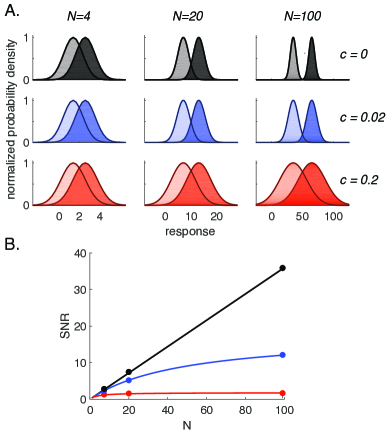
Figure 1: Dependence of the signal-to-noise ratio on the number of neurons ($N$) and the correlation strength ($c$). A. Probability densities of the activity for several combinations of $N$ and $c$, in a homogenous population of neurons that respond somewhat more strongly to stimulus $A$ (darker shaded regions) than to stimulus $B$. For the purpose of illustration, neural responses are taken to be Gaussian. The overlap between the two distributions decreases steadily with $N$ in the case of independent neurons ($c=0$, black), but minimally in the case with $c=0.2$. B. Dependence of the signal-to-noise ratio on $N$. Closed circles indicate parameter values as in panel A.

Because of the form of the scaling with population size in Eq. (4), the effect of noise correlation can be strong even in relatively small populations with modest values of correlation. For example, in the presence of $10\%$ correlation ($c=0.1$, a typical value for cortical and retinal neurons), noise correlation has an appreciable effect already in a population of a few dozen neurons. For $N=100$, and assuming $p\left(\text{A}\right)-p\left(\text{B}\right)\approx p\approx 0.5$, the signal-to-noise ratio amounts to $9$, as opposed to $100$ for an independent population of neurons. For $N=1000$, the signal-to-noise ratio grows to $10$, as opposed to $1000$ for an independent population of neurons. More generally, while the signal-to-noise ratio increases by one unit for every independent neuron added, in a correlated population it increases by an amount $\left(1-c\right)/\left(1+Nc\right)^{2}$ when one neuron is added to a population with $N$ neurons. With typical values of $c\approx 0.1$, this quantity drops rapidly to zero in populations with more than $100$ neurons.

There are at least two other ways of intuiting this result. The signal-to-noise ratio acquires a factor of $N$ in its denominator because each neuron shares a fraction of its variability with all the other neurons in the population. As a result, any ‘error’ committed by a neuron will be enhanced by a factor of $N$, since neurons share their variability. Consequently, the variability in the population response will be greatly enhanced. In other words, positive correlation broadens the distribution of population responses. Yet another way to think about this result is that positive correlation induces neurons to respond similarly: it is as if positive correlation yields a reduced ‘effective size’ of the population, and, hence, suppresses the coding capacity. In the extreme case of $100\%$ correlation ($c=1$), all neurons in the population behave identically, and the population as a whole cannot code for any more information than a single neuron does.

It is instructive to see how the conclusions obtained from the simple model are reflected by a fundamental information theoretic quantity, the mutual (Shannon) information. There are several equivalent ways to express the mutual information; for our purposes we adopt the form

$$I=\left\langle\sum_{r}P\left(r\mid s\right)\log\left(\frac{P\left(r\mid s\right)}{\left\langle P\left(r\mid s\right)\right\rangle_{S}}\right)\right\rangle_{S},$$ (5)

where $r\equiv\left(r_{1},\ldots,r_{N}\right)$ is the vector of population response (or population activity), $s\in S$ denotes a stimulus (and $S$ is the set of possible stimuli), and $\left\langle\cdot\right\rangle_{S}$ indicates an average over all stimuli. In our simple model, there are two stimuli, $s=$ A or B, and $r$ labels the $2^{N}$ possible states of the population:

$$r=\left(n_{1},\ldots,n_{N}\right),$$ (6)

where $n_{i}=0$ if neuron $i$ is silent and $n_{i}=1$ if neuron $i$ is firing. In this case, assuming that the two stimuli are equiprobable,

$$\left\langle P\left(r\mid s\right)\right\rangle_{S}=\frac{1}{2}\left[P\left(r\mid\text{A}\right)+P\left(r\mid\text{B}\right)\right],$$ (7)

we can rewrite Eq. (5) as

$$I=H-\frac{1}{2}\sum_{r}\left[P\left(r\mid\text{A}\right)\log\left(1+\frac{P\left(r\mid\text{B}\right)}{P\left(r\mid\text{A}\right)}\right)+P\left(r\mid\text{B}\right)\log\left(1+\frac{P\left(r\mid\text{A}\right)}{P\left(r\mid\text{B}\right)}\right)\right],$$ (8)

where $H=\log\left(2\right)=1$ bit of information associated with the stimulus.

The second term on the right-hand-side of Eq. (8) is referred to as the noise entropy and is a measure of the variability in the neural response that is not due to the variability in the stimulus. In other words, this term quantifies the amount of uninformative variability in the response. The noise entropy is a sum of terms, each of which corresponds to a particular realization of the population activity. From Eq. (8), it appears immediately that a given term vanishes if either of the conditional response probabilities, $P\left(r\mid\text{A}\right)$ or $P\left(r\mid\text{B}\right)$, vanishes; indeed, if a given stimulus prevents a particular activity pattern, the latter is informative—it ‘codes’ for the other stimulus. Thus, the noise entropy grows as the overlap between the two conditional response probabilities increases, and, correspondingly, the mutual information is suppressed. If the overlap of the conditional distributions does not decrease as $N$ increases, then the mutual information, $I$, saturates and never reaches the stimulus entropy, $H$. In this case, it is impossible to recover the full information about the stimulus from the neural population response even in an infinitely large population, in agreement with the picture from consideration of the signal-to-noise ratio.

4 Broader views: coding in heterogeneous neural populations with structured correlated noise

Because neurons all come with identical properties in our simple model, there is a single informative quantity: the total spike count, $k$ (Eq. (1)). More generally, information is represented in a higher-dimensional variable. Multiple studies (Abbott & Dayan, 1999, Sompolinsky et al., 2001, Wilke & Eurich, 2002, Romo et al., 2003, Golledge et al., 2003, Averbeck & Lee, 2003, Shamir & Sompolinsky, 2004, 2006, Averbeck & Lee, 2006, Averbeck et al., 2006, Josic et al., 2009, Ecker et al., 2011, Hu et al., 2014, Azeredo da Silveira & Berry II, 2014, Moreno-Bote et al., 2014, Franke et al., 2016, Zylberberg et al., 2016) have explored how noise correlation can affect the neural code in this case, by exploiting higher-dimensional versions of the structure illustrated in Fig. 1. The main—and important—departure from our simple model was the generalization to heterogeneous neural populations: the average single-neuron response to a given stimulus was assumed to vary from neuron to neuron, and likewise pairwise correlations were different from pair to pair. Most studies started with a set of ‘tuning curves’ (average response as a function of stimulus parameter) assigned to the neurons in the population. Noise, including pairwise correlations, was either estimated from neural recordings or posited on theoretical grounds. The fidelity of the population code was then evaluated in terms of a chosen figure of merit, such as the mutual information or a decoding error variance. The results obtained thus depended on the specifics of the assumptions involved in setting the forms of the tuning curves and of the noise model; to explore a range of behaviors, the latter had to be varied. For example, many early investigations used model neurons responding to a continuous stimulus with broad tuning curves, and assumed noise models in which the pairwise correlation depended only upon the tuning preferences of the two neurons in the pair. Later studies included more sophisticated forms of heterogeneity and dependences, such as the dependence of the pairwise correlation not only upon the tuning preferences but also upon the stimulus itself.

To illustrate how coding depends on the manner in which neurons are correlated, we take a more general but more qualitative approach. As stimulus parameters are varied, the responses of the $N$ neurons in the population trace out a hypersurface in the $N$-dimensional space of the population responses (Fig. 2A). If the tuning curves are sufficiently smooth, this hypersurface can be approximated locally by a hyperplane. (There exist important examples in which this approximation is not valid (Sreenivasan & Fiete, 2011, Blanco Malerba et al., 2020).) Single-trial population responses depart from this hyperplane due to noise; the orientation of the hyperplane and the geometry of the noise define $M$ ‘informative dimensions’ or ‘informative modes’,

$$m_{i}={\displaystyle\sum\limits_{j=1}^{N}}a_{ij}r_{j},$$ (9)

where $a_{ij}$ are numerical prefactors and $i=1,\ldots,M$. One can think of these variables as chosen to maximize the mutual information with the stimulus or to correspond to optimal decoding dimensions. If the noise is isotropic in the $N$-dimensional space of population responses, then the informative dimensions coincide with the hyperplane defined by the tuning curves; in general, however, the ‘informative hyperplane’ (defined by the coefficients $a_{ij}$) and the ‘signal hyperplane’ are distinct (Fig. 2C).

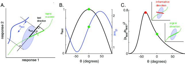
Figure 2: Signal and noise together define the informative direction for neural coding. A. Two-neuron illustration of quantities relevant for defining the signal-to-noise ratio in a specific direction. The thin green line illustrates how the signal changes as the stimulus is varied. The blue ellipse illustrates the distribution of noisy responses corresponding to a mean response located at one point along the green line. The signal-to-noise ratio along a test direction (black) at an angle $\theta$ relative to the signal direction can then be determined from the projection, $s_{test}$, of the signal vector, $s$, and the projection of the noise, $\sigma_{test}$ in the test direction. B. Signal and noise as a function of the angle between the test and signal directions, for the situation depicted in panel A. The green circles occur when the test and signal directions are the same. C. The signal-to-noise ratio as a function of $\theta$. Insets show the signal direction (green) and the informative direction, the direction that maximizes the signal-to-noise ratio (red).

In the simplest and most commonly studied case of a one-dimensional stimulus, the informative mode,

$$m={\displaystyle\sum\limits_{j=1}^{N}}a_{j}r_{j},$$ (10)

lies along the vector with elements $a_{j}$. The quantity in Eq. (10) plays a role analogous to the spike count (Eq. (1)) in our simple model. By analogy with the simple model, the ‘strength of the signal’ carried by the informative mode is obtained by averaging over the noise, and grows linearly with the size of the population: $\left\langle m\right\rangle\sim\mathcal{O}\left(N\right)$. How much information a mode represents depends also upon the uncertainty of its value. Early studies considered cases in which this uncertainty, as measured by its variance, grew either linearly or quadratically with $N$ (Abbott & Dayan, 1999, Sompolinsky et al., 2001, Wilke & Eurich, 2002, Romo et al., 2003). If neurons are independent, the variance of the informative modes grows linearly with the size of the population, so that each mode can represent reliably up to about $\sqrt{N}$ different states of the stimuli. In this case, the mutual information grows logarithmically in $N$. If, however, positive correlation corrupts an informative mode, its typical amplitude grows linearly with the size of the population and its variance grows quadratically; in this case, the informative mode can represent reliably only $O\left(1\right)$ different states of the stimulus—i.e., the mutual information saturates to a finite value smaller than the stimulus entropy. More recent studies (Ecker et al., 2011, Hu et al., 2014, Azeredo da Silveira & Berry II, 2014, Franke et al., 2016, Zylberberg et al., 2016) (but see also Refs. (Abbott & Dayan, 1999, Wilke & Eurich, 2002)) introduced examples in which noise correlation may in fact suppress the variance of informative modes relative to the independent case, thereby enhancing the resolution of the code.

We can discuss these different cases by exploiting Eq. (10), which we can rewrite as

$$m ={\displaystyle\sum\limits_{i=1}^{N}}a_{i}\left\langle r_{i}\right\rangle+{\displaystyle\sum\limits_{i=1}^{N}}a_{i}\eta_{i}$$

$$\equiv\left\langle m\right\rangle+\mu,$$ (11)

where $\left\langle\cdot\right\rangle$ denotes an average over the noise and the $\eta_{j}$s are $N$ correlated random variables with vanishing mean. The second term, $\mu$, represents the uncertainty on the magnitude of the informative mode and is the projection of the population noise along the informative direction defined by the vector with elements $a_{j}$ (Fig. 2). The informative mode can encode about as many different states of the stimulus as the ratio between the first term, $\left\langle m\right\rangle$, and the standard deviation of the second term, $\mu$, in Eq. (11). Its variance is calculated as

$$\left\langle\mu^{2}\right\rangle ={\displaystyle\sum\limits_{i=1}^{N}}a_{i}^{2}\left\langle\eta_{i}^{2}\right\rangle+{\displaystyle\sum\limits_{i=1}^{N}}a_{i}{\displaystyle\sum\limits_{i\neq j}}a_{j}\left\langle\eta_{i}\eta_{j}\right\rangle$$

$$={\displaystyle\sum\limits_{i=1}^{N}}a_{i}\left(a_{i}\left\langle\eta_{i}^{2}\right\rangle+Q_{i}\right),$$ (12)

where

$$Q_{i}={\displaystyle\sum\limits_{i\neq j}}a_{j}\left\langle\eta_{i}\eta_{j}\right\rangle.$$ (13)

The first term in Eq. (12) represents the contribution of independent neuron variance, and the second term represents the contribution of correlated variability among neurons. Generically, $Q_{i}$ can behave as a function of the population size in one of four ways, listed as follows.

(i) $Q_{i}=0.$

(ii) $Q_{i}\approx\pm a_{i}\left\langle\eta^{2}\right\rangle\tilde{n}c.$

(iii) $Q_{i}\approx a_{i}\left\langle\eta^{2}\right\rangle\tilde{N}c.$

(iv) $Q_{i}\approx-a_{i}\left\langle\eta^{2}\right\rangle\tilde{N}c.$

Here, $\left\langle\eta^{2}\right\rangle$ corresponds to the typical scale of the single-cell variance and $c\sim O\left(1\right)>0$ corresponds to the typical scale of the (positive) pairwise noise correlation. The quantity $Q_{i}$ also depends on an ‘effective population size’ ($\tilde{n}$ or $\tilde{N}$) that corresponds to the magnitude of the correlated noise mode relevant to coding. Generically, $\tilde{n}\sim O\left(1\right)>0$ and $\tilde{N}\sim O\left(N\right)>0$ are constants; in particular regimes, $\tilde{N}$ can scale more weakly with $N$ (see below). Without loss of generality, we exhibit a prefactor $a_{i}$ in these expressions, for the sake of convenience given the form of Eq. (12). This form is natural, also, in the case of most models considered in the literature, in which the total spike count in the population is uninformative. For example, for neurons with broad tuning curves that tile the stimulus space densely, so that the total spike count in the population is roughly independent of the stimulus, the elements of the informative vector sum to zero, i.e., $\sum_{i=1}^{N}a_{i}=0$. In a population with uniform correlations (Abbott & Dayan, 1999, Wilke & Eurich, 2002), i.e., $\left\langle\eta_{i}\eta_{j}\right\rangle=\left\langle\eta^{2}\right\rangle c$ for all $i,j$, the quantity $Q_{i}$ amounts to $-a_{i}\left\langle\eta^{2}\right\rangle c$.

We can now organize the various results which appear in the literature among these four categories:

1. Independence (case i). If neurons are independent, $\left\langle\mu^{2}\right\rangle$ grows like $N$, so that the informative mode can represent about $\left\langle m\right\rangle/\sqrt{\left\langle\mu^{2}\right\rangle}\sim\sqrt{N}$ different states of the stimulus.

2. Strongly detrimental noise correlation (case iii). Early models (Abbott & Dayan, 1999, Sompolinsky et al., 2001, Wilke & Eurich, 2002), assume smooth, broad tuning curves, so that a given stimulus activates most neurons in the population. As a result, the informative vector contains a macroscopic fraction of non-vanishing elements, $a_{i}$, which vary slowly with $i$. If the covariance of the noise, $\left\langle\eta_{i}\eta_{j}\right\rangle$, also varies slowly with $j$ over the population, it can ‘interfere constructively’ with $a_{j}$, meaning that the noise is large in directions in which the informative mode is also large. In this case, $Q_{i}$ grows like $N$ and $\left\langle\mu^{2}\right\rangle$ grows like $N^{2}$, and the informative mode can represent only $\mathcal{O}\left(1\right)$ different states of the stimulus. In other words, the performance of the code (as measured, e.g., by the mutual information) saturates for large neural populations.

3. Weakly detrimental or weakly beneficial noise correlation (case ii). Some early studies (Abbott & Dayan, 1999, Wilke & Eurich, 2002) noted that noise correlations that are uniform over the population can lead to an improvement in the coding performance. Indeed, if $\left\langle\eta_{i}\eta_{j}\right\rangle=\left\langle\eta^{2}\right\rangle c$ is independent of $i$ and $j$, then $Q_{i}=-a_{i}\left\langle\eta^{2}\right\rangle c$, and

$$\left\langle\mu^{2}\right\rangle=\sum_{i=1}^{N}a_{i}^{2}\left\langle\eta^{2}\right\rangle\left(1-c\right)\sim\left(1-c\right)\mathcal{O}\left(N\right).$$ (14)

As a result, the informative mode can represent a number of different states of the stimulus that depends upon the population size and the strength of the noise correlation as $\sqrt{N}/\left(1-c\right)$. This moderate improvement of the coding performance was obtained in studies that allowed allowed for neuron-to-neuron variability in tuning curve properties (Shamir & Sompolinsky, 2006, Ecker et al., 2011). This variability implied rapid fluctuations of the elements of the informative vector, $a_{i}$, as a function of the neuron index, $i$. If, by contrast, the noise covariance, $\left\langle\eta_{i}\eta_{j}\right\rangle$, varies smoothly over the population, then the ‘destructive interference’ between these two terms yields, again, a linear scaling of $Q_{i}$ with $N$, similar to the case of perfectly uniform correlation. More generally, whether the noise correlation is strongly detrimental or weakly detrimental/beneficial depends upon whether the interference between informative vector and noise covariance is constructive or destructive, respectively, over the population.

4. Strongly beneficial noise correlation (case iv). Recent studies noted that the ‘destructive interference’ between the elements of the informative vector and the noise covariance can lead to an appreciable suppression of the uncertainty (Azeredo da Silveira & Berry II, 2014, Franke et al., 2016, Zylberberg et al., 2016). This occurs if $a_{j}$ and $\left\langle\eta_{i}\eta_{j}\right\rangle$ both vary slowly as a function of $j$, over the population, but are, roughly speaking, ‘out of phase’: positive noise correlations are suppressed for neurons which contribute to a greater degree to the ‘strength of the signal’, and vice versa. As a consequence, the quantity $Q_{i}$ becomes negative and scales with $N$  and the variance of the noise is calculated as

$$\left\langle\mu^{2}\right\rangle\approx\alpha N\left\langle\eta^{2}\right\rangle\left(1-\tilde{N}c\right),$$ (15)

where $\alpha$ is a positive number of $O\left(1\right)$ and $c$ is the typical scale of the (positive) pairwise noise correlation as before. Generically, $\tilde{N}$ scales linearly with $N$, so that uncertainty is strongly suppressed by noise correlation, through the term $1-\tilde{N}c$. The informative mode can then represent a number of different states of the stimulus that depends upon the population size and the strength of the noise correlation as $\sqrt{N}/\left(1-\tilde{N}c\right)$. The important point, here, is that the denominator is strongly suppressed as a function of population size. This results, in particular, in an appreciable enhancement of the coding performance when $\tilde{N}\sim O\left(1/c\right)$.

The right-hand-side of Eq. (15) remains non-negative since the covariance of the noise is positive semi-definite. In this formulation, we assume that the scale of the correlation, characterized by $c$, is fixed; as $\tilde{N}$ increases, the covariance matrix becomes increasingly constrained by this condition, and, depending on its structure, one or several small eigenvalues may emerge. As these tend to zero, the informative vector rotates with respect to the eigenvectors of the noise covariance matrix and, as a consequence, the scaling of $\tilde{N}$ becomes weaker. This limiting regime in the vicinity of a singular noise covariance matrix interpolates between the scalings in cases (ii) and (iv), thereby allowing the term $1-\tilde{N}c$ in Eq. (15) to remain non-negative. We return to the discussion of the behavior of the informative direction as a function of the structure of the noise in Sec. 6, where we provide further illustration in a concrete model.

The dependence of this boost upon the population size is a signature of the collective effect at play here: in a correlated system, the behavior of a neuron is affected by all  $N-1$ other neurons. For $c\sim 0.1$, as observed experimentally, the effect of correlation upon coding is appreciable already in populations as small as tens or hundreds of neurons (Azeredo da Silveira & Berry II, 2014). A specific incarnation of this phenomenon occurs in a model of broadly tuned neurons in which the dependence of the correlation between a pair of neurons upon the difference in their tuning preference is allowed to be non-monotonic (Franke et al., 2016, Zylberberg et al., 2016).

The list just outlined catalogs the various ways in which noise correlation can affect the coding of stimuli along an informative dimension by shaping the variability in the population response. Our discussion of the ‘interference’ between elements of the informative vector and the noise covariances can be seen as a generalization of the ‘sign rule’ (Hu et al., 2014), according to which positive correlation is favorable in a pair of neurons with negative signal correlation, and vice versa.

There is one case, however, which was not covered: this is when there is no informative dimension in the sense we discussed above. To be specific, consider the case in which the average magnitude of the activity in the ‘informative’ dimension, $\left\langle m\right\rangle$, is independent of the stimulus. Information about the stimulus can be encoded in the noise itself: if correlation depends upon the stimulus, then different patterns of population activity can discriminate stimuli. We return to this case in the next section, in a more systematic treatment of the mutual information.

Finally, above we have considered only pairwise correlations. In the presence of higher-order correlations, additional kinds of scalings occur. If real neural systems are dominated by the strong co-activation of groups of neurons corresponding to higher-order correlation, the analyses developed so far may have a limited relevance to our understanding of population coding.

5 A general approach to account for the impact of noise correlations on mutual information

Many of the studies of neural population coding to date have relied upon specific models of neural populations, and have focused on one central question: how does the coding performance scale with the number of neurons, in particular in the limit of large populations? Moreover, most of these studies quantified coding through the Fisher information. Other information-theoretic quantities, such as the mutual (Shannon) information, are more fundamental (Cover, 1999, Brunel & Nadal, 1998, Kang & Sompolinsky, 2001, Wei & Stocker, 2016) and avoid difficulties associated with the Fisher information (Bethge et al., 2002). The Fisher information is local in stimulus space, whereas the mutual information quantifies the accuracy of stimulus representation over the entire stimulus space. The use of the Fisher information also relies upon some restrictive assumptions, and yields only a lower bound on the coding resolution, which may or may not be tight.

Coding in neural populations can be examined from a general perspective by expressing the mutual information in a form that isolates the impact of different types of correlation (Panzeri et al., 1999, Pola et al., 2003). We discuss the implications of this decomposition here; in App. B, we provide a derivation of the decomposition, which follows and somewhat simplifies that in Refs. (Panzeri et al., 1999, Pola et al., 2003). The central result is a reformulation of the mutual information as a sum of three terms:

$$I=I_{\text{independent}}+I_{\text{correlated}}^{\left(1\right)}+I_{\text{correlated}}^{\left(2\right)}.$$ (16)

Each of the terms can be expressed as a function of the joint probability, $P\left(r,s\right)$, between stimulus, $s$, and population response, $r$, and transformations of this joint probability, such as $P_{0}\left(r\mid s\right)$, defined in Eq. (31) which denotes the conditional probability of the response in a population of independent neurons with matched mean and variance. In App. B, we show that the three terms in Eq. (16) can be written as

$$I_{\text{independent}}\equiv\left\langle\sum_{r}P_{0}\left(r\mid s\right)\log\left(\frac{P_{0}\left(r\mid s\right)}{\left\langle P_{0}\left(r\mid s\right)\right\rangle_{S}}\right)\right\rangle_{S},$$ (17)

$$I_{\text{correlated}}^{\left(1\right)}=\left\langle\sum_{r}P\left(r\mid s\right)\log\left(\frac{P\left(r\mid s\right)/P_{0}\left(r\mid s\right)}{\left\langle P\left(r\mid s\right)\right\rangle_{S}/\left\langle P_{0}\left(r\mid s\right)\right\rangle_{S}}\right)\right\rangle_{S}$$ (18)

and

$$I_{\text{correlated}}^{\left(2\right)}=\left\langle\sum_{r}\left[P\left(r\mid s\right)-P_{0}\left(r\mid s\right)\right]\log\left(\frac{\prod_{i=1}^{N}P\left(r_{i}\right)}{\left\langle P_{0}\left(r\mid s\right)\right\rangle_{S}}\right)\right\rangle_{S}.$$ (19)

The benefit of this reformulation of the mutual information is that each of these three terms come with a transparent interpretation. The term $I_{\text{independent}}$ represents the information carried by conditionally independent neurons; indeed, if there is no noise correlation, $P\left(r\mid s\right)=P_{0}\left(r\mid s\right)$, and both $I_{\text{correlated}}^{\left(1\right)}$ and $I_{\text{correlated}}^{\left(2\right)}$ vanish. Thus, $I_{\text{independent}}$ accounts for the amount of information carried by the population which is not affected by noise correlations. In App. B, we show that $\ I_{\text{independent}}$ can be broken down further to isolate the impact of signal correlations.

The term $I_{\text{correlated}}^{\left(1\right)}$ is the formal analog to the term $I_{\text{independent}}$, but where the information is carried by noise correlations rather than by the structure of mean response. Thus, it accounts for stimulus coding by the noise correlations themselves: the same way differential firing rates characterize different stimuli, non-uniform noise correlation can also specify the stimulus. Figure 3B illustrates an example of the effects captured by this term in the simple case of a two-neuron population that encodes a binary stimulus, $s=$ A or B. Here, the mean responses to stimuli A and B are identical, yet the identity of the stimulus can be inferred from the two-neuron response due to the differences in noise correlation. Generalizations of this mechanism have been studied in various models of neural population coding (Shamir & Sompolinsky, 2004, Josic et al., 2009, Zylberberg, 2018), and stimulus-dependence of correlations has been proposed as supporting visual coding in direction-selective middle-temporal neurons in monkeys (Ponce-Alvarez et al., 2013). As we show in App. B, both terms $I_{\text{independent}}$ and $I_{\text{correlated}}^{\left(1\right)}$ are non-negative; they capture occurrences in which variations of mean response or noise correlations as a function of stimulus are informative.

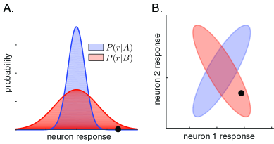
Figure 3: Representation of information by stimulus-dependent noise. A. Illustration of a situation in which the variance of the response of a single neuron encodes information about the stimulus identity. For example, the noisy response denoted by the black circle is more likely to be induced by stimulus $B$ than by stimulus $A$. B. Illustration of a similar situation, in which the information is encoded in correlations of the noise in the joint response of two neurons. In both panels A and B, the mean response is the same for stimulus A and stimulus B, and, hence, uninformative about their identity.

Finally, $I_{\text{correlated}}^{\left(2\right)}$ represents the increment or decrement of information due to the interplay between signal correlation and noise correlation. From Eq. (19), it is apparent that $I_{\text{correlated}}^{\left(2\right)}$ vanishes if either noise correlation is absent ($P\left(r\mid s\right)=P_{0}\left(r\mid s\right)$) or signal correlation is absent ($\left\langle P_{0}\left(r\mid s\right)\right\rangle_{S}=\prod_{i=1}^{N}P\left(r_{i}\right)$). Furthermore, and unlike the other two components of the mutual information, this component can be positive or negative. For a given stimulus, $s$, each population response, $r$, yields a positive contribution if $\left[P\left(r\mid s\right)-P_{0}\left(r\mid s\right)\right]\times\left[\prod_{i=1}^{N}P\left(r_{i}\right)-\left\langle P_{0}\left(r\mid s\right)\right\rangle_{S}\right]$ is positive, and a negative contribution otherwise. In other words, the contribution to the information of a population response is positive if noise correlation favors this population response while signal correlation disfavors it, and vice versa, and it is negative if both noise and signal correlations either favor or disfavor the population response. (When we say ‘favor’ and ‘disfavor’, as usual we are comparing the case of a population of correlated neurons to the case of a population of independent neurons.) The form of $I_{\text{correlated}}^{\left(2\right)}$ in Eq. (19) captures another generalized formulation of the sign rule we mentioned in the previous section (Hu et al., 2014). It also illustrates in the language of mutual information, and without reference to any specific model, the kind of ‘constructive versus destructive interference’ discussed in the previous section.

The reader might wonder about the merits of what may seem like a mere mathematical exercise. Many studies today start from data and end in data, and seek to make sense of data rather than to propose a theoretical framework. In this context, we find it refreshing to examine the question from a more abstract theoretical point of view, not tied to a specific model. It adds to our understanding to be able to consider a same neural mechanisms from multiple points of view. Having said this, we emphasize that the framework just outlined can indeed be put to the task of analyzing data. It was recently used, for example, to uncover the organization of assemblies of neurons with redundant and synergistic coding of visual information in monkey cortex (Nigam et al., 2019).

6 Information coding and the geometry of noise correlation

The breakdown of the mutual information discussed in the previous section teases apart the various contributions from signal and noise correlations, but it provides neither a quantitative nor a geometrical view of how the structures of signal and noise together impact coding. This section develops such a geometrical view by revisiting the task of discriminating two stimuli, A and B, discussed in Sec. 3.

To streamline the mathematical treatment, we consider a limiting case in which the mutual information takes a simple form, namely, the case in which stimulus A is presented with probability $\phi\ll 1$. In this limit, the mutual information can be written as

$$I=\phi\sum_{r}P\left(r\mid\text{A}\right)\ln\left(\frac{P\left(r\mid\text{A}\right)}{P\left(r\mid\text{B}\right)}\right)+\mathcal{O}\left(\phi^{2}\right),$$ (20)

where $r$ is the vector of neural responses, $r^{T}=\left(r_{1},\ldots,r_{N}\right)$. This approximation is valid when $\phi P\left(r\mid\text{A}\right)/P\left(r\mid\text{B}\right)\ll 1$  i.e., we exclude cases in which there exist responses overwhelmingly more likely to be elicited by stimulus A than by stimulus B. This condition is satisfied, in particular, in the case of a demanding discrimination task, since in this case the distributions $P\left(r\mid\text{A}\right)$ and $P\left(r\mid\text{B}\right)$ overlap considerably. If the noise is Gaussian, the mutual information can be expressed in terms of the response mean and covariance, as

$$I=\phi\ln\left(\frac{\operatorname*{Det}\left(C_{\text{A}}\right)}{\operatorname*{Det}\left(C_{\text{B}}\right)}\right)+\frac{1}{2}\phi\operatorname*{Tr}\left(C_{\text{A}}C_{\text{B}}^{-1}-\mathcal{I}\right)+\frac{1}{2}\phi m^{T}C_{\text{B}}^{-1}m,$$ (21)

where $C_{s}$ ($s=\text{A,B}$) is the covariance of the noise in response to stimulus $s$, $\mathcal{I}$ is the identity matrix, and $m$ is the ‘signal vector’ which, in this case, is simply the difference between the mean responses to the two stimuli, i.e.,

$$m_{i}\equiv\left\langle r_{i}\right\rangle_{\text{A}}-\left\langle r_{i}\right\rangle_{\text{B}}.$$ (22)

Here $i$ indicates the $i$th neuron, and $\left\langle\cdot\right\rangle_{s}$ denotes the average over the conditional probability, $P\left(r\mid s\right)$. To obtain Eq. (21), we have further assumed that the spike counts take large values, so that their discrete nature becomes unimportant and the sum over population patterns can be replaced by an integral.

Equation (21) can be interpreted particularly transparently in the case in which the variances of the single-neuron responses do not depend on the stimulus. In this case, the first two terms depend only upon the noise correlation; they correspond to the term $I_{\text{correlated}}^{\left(1\right)}$ in Eq. (16). The third term in Eq. (21) describes the interplay between signal and noise correlation, and corresponds to the term $I_{\text{correlated}}^{\left(2\right)}$ in Eq. (21). This term is the formal equivalent to the so-called ‘linear Fisher information’ used in many earlier studies. It can also be viewed as the signal-to-noise ratio discussed in Sec. 3, or the square of the sensitivity index, $d^{\prime}$.

We can examine the contribution of the interplay of signal and noise correlation by comparing the third term in Eq. (21) for correlated and independent neurons, again in the case in which the single-neuron variances do not depend on the stimulus. For independent neurons, the mutual information reduces to

$$I_{0}\equiv\frac{1}{2}\phi m^{T}C_{0}^{-1}m,$$ (23)

where $C_{0}$ is the diagonal matrix obtained from $C_{\text{B}}$ by setting all off-diagonal elements to zero. If neurons are recorded from individually, one has access only to the moments $m$ and $C_{0}$, and the mutual information is estimated according to Eq. (23). By contrast, when neurons in a population are recorded from simultaneously, and the statistics of the population responses are fitted to a multivariate Gaussian, then the mutual information is given by the richer Eq. (21).

Since the covariance matrix in Eq. (23) is diagonal, the mutual information for independent neurons can be rewritten as

$$I_{0}=\frac{1}{2}\phi\sum_{i=1}^{N}\frac{m_{i}^{2}}{\sigma_{i}^{2}},$$ (24)

where $\sigma_{i}^{2}$ is the variance of the activity of neuron $i$. $I_{0}$ grows linearly as $N$ increases—a property of the limit of a rare stimulus considered here. (Beyond a crossover size, the first-order expansion in $\phi$ breaks down, and, asymptotically, the mutual information increases logarithmically in $N$). By analogy with Eq. (24), a natural way to calculate $I_{\text{correlated}}^{\left(2\right)}$, indeed an approach followed by much of the literature (starting with Refs. (Abbott & Dayan, 1999, Sompolinsky et al., 2001, Wilke & Eurich, 2002)), is to diagonalize the covariance matrix, to obtain

$$I_{\text{correlated}}^{\left(2\right)}=\frac{1}{2}\phi\sum_{i=1}^{N}\frac{\tilde{m}_{i}^{2}}{\lambda_{i}},$$ (25)

where $\tilde{m}_{i}$ are the elements of the vector $m$ in the new basis in which $C_{\text{B}}$ is diagonal, and $\lambda_{i}$ is the $i$th eigenvalue of the covariance matrix $C_{\text{B}}$. The argument is then that, if the structure of pairwise correlations is such that the eigenvectors of the covariance matrix (the ‘correlated modes’) are not sparse and involve contributions from a sizable fraction of the neurons in the population, then the eigenvalues will scale with the population size. In this case, the sum in Eq. (25) will yield a weaker scaling with $N$ than the sum in Eq. (24). In particular, if a few eigenvalues remain small as $N$ increases, then these eigenvalues dominate the sum in Eq. (25) and the latter asymptotes to a constant. In other words, $I_{\text{correlated}}^{\left(2\right)}$ saturates to a finite value in arbitrary large populations of neurons.

This approach is not entirely satisfactory because it is difficult to compare Eq. (24) and Eq. (25) since both the numerator and the denominator differ. Indeed, the numerator in Eq. (25) depends upon the signal vector as well as the structure of the noise covariance. Furthermore, some of the eigenvalues in Eq. (25) may take small values, and one may wonder what dominates the sum: the larger terms associated with small eigenvalues or the more numerous, smaller terms associated with larger eigenvalues. To resolve these ambiguities, it is possible instead calculate an ‘information ratio’ that quantifies by how much noise correlations suppress or enhance coding as compared to the case of an independent population of neurons (Azeredo da Silveira & Rieke, 2020). This ratio can be expressed in a compact form, as

$$R_{I}\equiv\frac{I_{\text{correlated}}^{\left(2\right)}}{I_{0}}=\frac{\operatorname*{Det}\left(\tilde{\chi}\right)}{\operatorname*{Det}\left(\chi\right)},$$ (26)

where $\chi$ is the correlation matrix corresponding to the covariance matrix $C_{\text{B}}$, and $\tilde{\chi}$ is the projection of $\chi$ on the $\left(N-1\right)$-dimensional subspace orthogonal to the modified signal vector, $v$, with elements $v_{i}\equiv m_{i}/\sigma_{i}$. The information ratio depends upon the spectra of the two matrices, $\chi$ and $\tilde{\chi}$. While $\chi$ depends only upon noise correlation, $\tilde{\chi}$ incorporates an interaction between the noise correlation the modified signal vector.

To intuit the behavior of the information ratio defined in Eq. (26), it is instructive to examine information coding with two correlated neurons. The covariance of the noise reads

$$C_{\text{B}}=\left(\begin{array}[c]{cc}\sigma_{1}^{2}&\sigma_{1}\sigma_{2}c\\ \sigma_{1}\sigma_{2}c&\sigma_{2}^{2}\end{array}\right),$$ (27)

where $\sigma_{1}$ and $\sigma_{2}$ are the standard deviations in the activities of the two neurons, and $c$ is the correlation of the noise. In this simple case, the information ratio takes the form

$$R_{I}=\frac{1-2c/\left(\zeta+\zeta^{-1}\right)}{1-c^{2}},$$ (28)

where

$$\zeta\equiv\frac{m_{1}}{\sigma_{1}}\left(\frac{m_{2}}{\sigma_{2}}\right)^{-1}.$$ (29)

Since the parameter $\zeta$ can take any real value, inspection of the form of the information ratio reveals that large volumes in the space of model parameters yield $R_{I}>1$ and, conversely, $R_{I}<1$. Specifically, the information ratio is larger than unity, i.e., noise correlation is beneficial to information coding, when $c>2/\left(\zeta+\zeta^{-1}\right)$. This relation, again, can be viewed as a generalization of the ‘sign rule’: it dictates how strong correlation ought to be to benefit coding as a function of the signal vector and the single-neuron variances.

This simple example also helps shed light on the discussion in Sec. 4. There, we invoked an ‘informative dimension’. Similarly, here, we can ask whether there is an especially informative dimension in the two-dimensional space of the two-neuron population activity: in which direction should the unit vector, $e$  point in order to maximize the mutual information $I\left(s;x\right)$, where $s=$ A or B and $x\equiv e^{T}m=e_{1}m_{1}+e_{2}m_{2}$? This problem is solved easily, and the unit vector that maximizes $I\left(S;x\right)$, call it $e^{\ast}$, can be expressed in terms of the signal vector as well as the variances and correlation of the pair of neurons. What is more interesting, though, is that the mutual information $I\left(S;x=e^{\ast T}m\right)$ matches $I_{\text{correlated}}^{\left(2\right)}$ exactly: that is, the one-dimensional variable $x$ recovers the entirety of the useful information contained in the two-dimensional activity of the neuron pair. The dimension defined by the vector $e^{\ast}$ in the space of population activity is thus an ‘informative dimension’ in the sense of Sec. 4.

In general, the informative dimension does not align with the signal vector. For example, in the limit of weak correlation, $\left|c\right|\ll 1$, and comparable variances, $\left|\sigma_{2}/\sigma_{1}-1\right|\ll 1$, the informative dimension is obtained by rotating the signal vector by an angle $c\left(m_{2}^{2}-m_{1}^{2}\right)/m^{2}-2\left(\sigma_{2}/\sigma_{1}-1\right)m_{1}m_{2}/m^{2}$. The fidelity of coding depends upon the noise along this direction, i.e., the variance of the projection of the noise along $e^{\ast}$. A contrasting picture has been discussed in the literature in recent years: a number of authors have argued that the fidelity of coding depends, rather, on the presence of what they call ‘differential correlations’ (Moreno-Bote et al., 2014, Kohn et al., 2016). These are taken to be present if the covariance matrix of the noise in the population activity contains a component proportional to $mm^{T}$—i.e., a component along the signal direction (Fig. 2A). The central conclusion from this line of research is that differential correlations limit coding performance in that they cause the information represented in the neural population to saturate asymptotically, as $N\rightarrow\infty$.

A picture that emerges from the argument summarized in this section and illustrated in Fig. 2 is that, if the covariance matrix contains small eigenvalues, then the information represented in the neural population (equivalently, the signal-to-noise ratio) can be large. This holds even if there is appreciable noise along the signal vector, provided that the eigenvectors corresponding to the low-noise directions are not orthogonal to the signal vector. More generally, figures of merit of the coding performance of a population of neurons, such as the mutual information or the signal-to-noise ratio, depend upon the full structure of the noise covariance in relation to the signal vector, and not exclusively upon the projection of the noise along the dimension defined by the signal vector. Rather, in scenarios such as the ones discussed above, what matters is the projection of the noise along an informative dimension in general distinct from that along the signal vector. This is true in the case of finite values of $N$ and in the asymptotic limit with $N\rightarrow\infty$. While some of the mathematical statements can simplify in the asymptotic limit, this limit may be far from natural for neural systems; for example, individual neurons may receive input from a modest number of presynaptic neurons, and correlations in this collection of presynaptic neurons will shape signaling in the postsynaptic neuron.

7 Future directions

The discussion above aims at unifying various results in the literature using a common metric for neural coding—the mutual information. We build intuition about the impact of noise correlations on coding by developing a geometrical picture of the structure of signal and noise. Our goal is to highlight situations in which noise correlations are beneficial, detrimental, or inconsequential for the fidelity of the neural population code rather than to consider specific examples that fall into one category or another. Below, we summarize the assumptions that form the basis of our discussion and we touch upon some of the open questions that it raises.

Obstacles to understanding coding in populations of neurons arise largely from the high dimensionality of the problem. Experiments by necessity probe a small subregion of the space of interesting stimuli, and the presence of response nonlinearities (such as adaptation) imply that insights gleaned from such experiments often do not generalize to all stimuli. The space of neural responses is similarly high dimensional, and is impossible to probe completely in the finite duration of an experiment. But even an incomplete understanding of the role of noise correlations in neural responses is helpful to guide experimental design. For instance, understanding the neural code requires experiments that not only measure noise correlations but also take into account their relation to the encoded signal. Response variability may lie in a direction in which it impacts the encoded signal minimally. As an example, consider a population of orientation-tuned V1 neurons. A change in stimulus orientation will increase activity in some neurons and decrease activity in others. Noise that produces correlated fluctuations in firing rate that are uniform across the population will interact minimally with the signal created by changes in orientation.

Our discussion centers around correlations between pairs of neurons, and neglects higher-order correlations. This is a matter of practicality: pairwise correlations have been measured extensively while we know much less about the properties of higher-order correlations in real neural circuits. This is changing with the availability of experimental approaches that allow a large number of cells to be monitored simultaneously. Theoretical frameworks that account for geometrical relations between signal and higher-order noise correlations are likely to play an important role in the development of new experimental protocols and methods of data analyses, just as has been the case hitherto for pairwise correlations.

We chose to focus this review on how structures of signal and noise interact from a statistical point of view, rather than examining the neural mechanisms that produce such structures. Single-cell properties and the connectivity of real circuits constrain the structure of both signal and noise, and a finer understanding of the connection between biological constraints and network properties, on the one hand, and the statistics of population response, on the other, will help interpret empirical observations (Doiron et al., 2016, Rosenbaum et al., 2017, Huang et al., 2019, Trousdale et al., 2012, Ocker et al., 2017, Ostojic et al., 2009, Mastrogiuseppe & Ostojic, 2018, Schuessler et al., 2020, Tannenbaum & Burak, 2017, Goris et al., 2014, Lin et al., 2015, Pernice et al., 2011, Pernice & da Silveira, 2018, de la Rocha et al., 2007, Vidne et al., 2012). A ubiquitous example is the divergence of a common input into parallel circuits, which can create both signal and noise correlations in those circuits. This is just one of the many ways in which real circuit mechanisms shape signal and noise. Returning to the picture of collective variables from statistical physics, we can hope in the future to understand the relation between the mechanisms that shape interactions between neurons, the impact of those interactions on the structure of signal and noise, and how these combine to yield a representation of information in neural populations.

Much of the literature in computational neuroscience focuses upon population coding in the ‘thermodynamic limit’ in which $N\longrightarrow\infty$, that is, the limit of large populations of neurons. This is not, however, the only relevant limit. Individual neurons receive input from a finite set of other neurons; what matters for the postsynaptic neuron is the representation of information in its finite presynaptic pool. From a mathematical point of view, also, populations of moderate sizes may be the relevant ones: for particular structures of pairwise noise correlation, the condition $Nc\approx 1$ defines a ‘strongly correlated regime’ in which stimuli can be encoded faithfully in the population activity of tens or hundreds of neurons. And higher-order correlation can further enhance the coding performance of ‘small’ populations. Ultimately, we would like to relate the coding accuracy in given populations of neurons to recorded perceptual acuity and behavioral biases and variability.

Historically, studies of noise correlation in neural activity were motivated precisely by questions of this type. A set of early papers proposed that noise correlations relieved the necessity to consider populations of more than a few hundred neurons, since the accuracy of the encoded information saturated (Zohary et al., 1994, Bair et al., 2001). More recent studies have shown that noise correlations can be beneficial for information coding (Averbeck & Lee, 2004, 2006, Montani et al., 2007, Graf et al., 2011, Lin et al., 2015, Franke et al., 2016, Zylberberg et al., 2016, Montijn et al., 2016), and that when correlations are detrimental the encoded information saturates in much larger populations of hundreds or thousands of neurons (Bartolo et al., 2020, Rumyantsev et al., 2020). One possible mechanism for this relative insensitivity of coding to noise is the alignment of modes of strongly correlated noise away from the signal direction (Bartolo et al., 2020, Rumyantsev et al., 2020). At least one recent (and unpublished) study (Stringer et al., 2019), however, suggests that mysteries still lie ahead. The authors show that information encoded in mouse visual cortex does not saturate in populations as large as 20000 neurons. Visual acuity inferred from activity in these large populations outperforms mouse behavior by a factor of 10. This study challenges our view of sensory coding. Mice may be able to improve, through learning, their use of the encoded information; if this is not the case, however, there may be fundamental reasons for which the brain relinquishes the use of some of the information it has encoded. A satisfactory understanding of information coding by neurons may only be possible through the combined study of encoding and decoding in the brain, and behavior.

Appendices

Appendix A Noise correlation versus signal correlation

When we consider the noisy response of a neural population to an ensemble of stimuli, there are two possible averaging procedures: we can calculate averages (moments) over the noise or over the ensemble of stimuli. Loosely speaking, the former yields noise correlation while the latter yields signal correlation. To be more specific, we consider a population of $N$ neurons and we denote their outputs by $r_{1},\ldots,r_{N}$. The statistics of population response is given by the conditional probability

$$P\left(r_{1},\ldots,r_{N}\mid s\right),$$ (30)

where $s$ refers to a stimulus chosen from a set of discrete stimuli or drawn from a density over continuous stimuli. Noise correlations are non-vanishing if

$$P\left(r_{1},\ldots,r_{N}\mid s\right)\neq{\displaystyle\prod\limits_{i=1}^{N}}P\left(r_{i}\mid s\right)\equiv P_{0}\left(r_{1},\ldots,r_{N}\mid s\right),$$ (31)

where $P\left(r_{i}\mid s\right)$ is obtained from $P\left(r_{1},\ldots,r_{N}\mid s\right)$ by averaging out all $r_{j}$, with $j\neq i$. The probability function in Eq. (30) specifies the noise correlations; these characterize the population variability in response to a given stimulus, and, hence, are themselves functions of the stimulus. By contrast, signal correlation is a property if the statistics of the population response over the ensemble or density of stimuli. Signal correlations are obtained from the probability function

$$\left\langle{\displaystyle\prod\limits_{i=1}^{N}}P\left(r_{i}\mid s\right)\right\rangle_{s}\equiv P_{0}\left(r_{1},\ldots,r_{N}\right),$$ (32)

where $\left\langle\cdot\right\rangle_{s}$ denotes an average over the ensemble or density of stimuli. Signal correlations are non-vanishing if

$$\left\langle{\displaystyle\prod\limits_{i=1}^{N}}P\left(r_{i}\mid s\right)\right\rangle_{s}\neq{\displaystyle\prod\limits_{i=1}^{N}}\left\langle P\left(r_{i}\mid s\right)\right\rangle_{s}.$$ (33)

Here, our focus will be on noise correlation and its effect upon sensory coding. Whenever we mention ‘pairwise correlation’ between two neurons labeled by $i$ and $j$, we refer to the quantity calculated as

$$c_{ij}=\frac{\left\langle\left(r_{i}-\left\langle r_{i}\right\rangle\right)\left(r_{j}-\left\langle r_{j}\right\rangle\right)\right\rangle}{\sqrt{\left\langle\left(r_{i}-\left\langle r_{i}\right\rangle\right)^{2}\right\rangle\left\langle\left(r_{j}-\left\langle r_{j}\right\rangle\right)^{2}\right\rangle}},$$ (34)

where the average denoted by $\left\langle\cdot\right\rangle$ is weighed by the conditional probability in Eq. (30). This correlation coefficient follows the usual definition of a covariance normalized by the corresponding standard deviations. By analogy, we can define pairwise signal correlation as

$$c_{ij}^{\text{signal}}=\frac{\left\langle\left(\left\langle r_{i}\right\rangle-\left\langle\left\langle r_{i}\right\rangle\right\rangle_{s}\right)\left(\left\langle r_{j}\right\rangle-\left\langle\left\langle r_{j}\right\rangle\right\rangle_{s}\right)\right\rangle_{s}}{\sqrt{\left\langle\left(\left\langle r_{i}\right\rangle-\left\langle\left\langle r_{i}\right\rangle\right\rangle_{s}\right)^{2}\right\rangle_{s}\left\langle\left(\left\langle r_{j}\right\rangle-\left\langle\left\langle r_{j}\right\rangle\right\rangle_{s}\right)^{2}\right\rangle_{s}}},$$ (35)

where the average denoted by $\left\langle\cdot\right\rangle_{s}$ is weighed by the ‘prior probability’ over stimuli, $P\left(s\right)$.

Appendix B Breakdown of the mutual information in terms of signal and noise

We follow Refs. (Panzeri et al., 1999, Pola et al., 2003) which introduce a breakdown of the mutual information in several terms that exhibit the various ways in which noise correlations may influence the coding performance. We spell out a somewhat modified derivation, here, as the latter is possibly a more direct one. We reformulate the mutual information (Eq. (5)) in a form that emphasizes the contributions of signal and noise correlations.

To achieve this, we invoke the independent (marginalized) probabilities defined in Eqs. (31) and (32), and rewrite the mutual information in terms of the independent conditional probability, $P_{0}\left(r\mid s\right)$, and ratios that carry the contribution of correlations, $P\left(r\mid s\right)/P_{0}\left(r\mid s\right)$ and $\left\langle P\left(r\mid s\right)\right\rangle_{S}/\left\langle P_{0}\left(r\mid s\right)\right\rangle_{S}$, as

$$I=\left\langle\sum_{r}P\left(r\mid s\right)\left[\log\left(\frac{P\left(r\mid s\right)/P_{0}\left(r\mid s\right)}{\left\langle P\left(r\mid s\right)\right\rangle_{S}/\left\langle P_{0}\left(r\mid s\right)\right\rangle_{S}}\right)+\log\left(\frac{P_{0}\left(r\mid s\right)}{\left\langle P_{0}\left(r\mid s\right)\right\rangle_{S}}\right)\right]\right\rangle_{S}.$$ (36)

We further separate independent probabilities from correlated ones by adding a subtracting to this quantity the mutual information corresponding to an independent population of neurons, i.e., the term

$$I_{\text{independent}}\equiv\left\langle\sum_{r}P_{0}\left(r\mid s\right)\log\left(\frac{P_{0}\left(r\mid s\right)}{\left\langle P_{0}\left(r\mid s\right)\right\rangle_{S}}\right)\right\rangle_{S}.$$ (37)

This manipulation allows us to to obtain the form in Eq. (16), i.e.,

$$I=I_{\text{independent}}+I_{\text{correlated}}^{\left(1\right)}+I_{\text{correlated}}^{\left(2\right)},$$ (38)

where $I_{\text{correlated}}^{\left(1\right)}$ is defined in Eq. (18) and

$$I_{\text{correlated}}^{\left(2\right)}=\left\langle\sum_{r}\left[P\left(r\mid s\right)-P_{0}\left(r\mid s\right)\right]\log\left(\frac{P_{0}\left(r\mid s\right)}{\left\langle P_{0}\left(r\mid s\right)\right\rangle_{S}}\right)\right\rangle_{S}.$$ (39)

The quantity $I_{\text{independent}}$ represents the information carried by conditionally independent neurons; indeed, if there is no noise correlation, $P\left(r\mid s\right)=P_{0}\left(r\mid s\right)$, and both $I_{\text{correlated}}^{\left(1\right)}$ and $I_{\text{correlated}}^{\left(2\right)}$ vanish. It can be broken down further, to extract the contribution from signal correlation, by bringing in the single-cell marginalized probabilities,

$$P\left(r_{i}\right)\equiv\left\langle P_{0}\left(r_{i}\mid s\right)\right\rangle_{s}.$$ (40)

With these, we can rewrite $I_{\text{independent}}$ as

$$I_{\text{independent}} =\left\langle\sum_{r}P_{0}\left(r\mid s\right)\log\left(\frac{P_{0}\left(r\mid s\right)}{\prod\nolimits_{i=1}^{N}P\left(r_{i}\right)}\right)\right\rangle_{S}-\left\langle\sum_{r}P_{0}\left(r\mid s\right)\log\left(\frac{\left\langle P_{0}\left(r\mid s\right)\right\rangle_{S}}{\prod\nolimits_{i=1}^{N}P\left(r_{i}\right)}\right)\right\rangle_{S}$$

$$=I_{\text{independent}}^{\left(1\right)}-I_{\text{independent}}^{\left(2\right)},$$ (41)

with

$$I_{\text{independent}}^{\left(1\right)}=\sum_{i=1}^{N}\left\langle\sum_{r}P_{0}\left(r_{i}\mid s\right)\log\left(\frac{P_{0}\left(r_{i}\mid s\right)}{\left\langle P_{0}\left(r_{i}\mid s\right)\right\rangle_{s}}\right)\right\rangle_{s}$$ (42)

and

$$I_{\text{independent}}^{\left(2\right)}=\sum_{r}\left\langle P_{0}\left(r\mid s\right)\right\rangle_{S}\log\left(\frac{\left\langle P_{0}\left(r\mid s\right)\right\rangle_{S}}{\prod_{i=1}^{N}\left\langle P_{0}\left(r_{i}\mid s\right)\right\rangle_{S}}\right).$$ (43)

By comparing the form of Eq. (42) with that of Eq. (5), we see that it expresses the sum over the information carried by $N$ independent neurons. Since $I_{\text{independent}}^{\left(2\right)}$ vanishes in the absence of signal correlation, $I_{\text{independent}}^{\left(1\right)}$ amounts to the total mutual information if both signal and noise correlations vanish. The quantity $I_{\text{independent}}^{\left(2\right)}$ thus represents the loss of information due signal correlation; indeed, $I_{\text{independent}}^{\left(2\right)}$ is nothing but the difference between the entropy of the marginalized independent distribution, $\prod_{i=1}^{N}\left\langle P_{0}\left(r_{i}\mid s\right)\right\rangle_{S}$, and the entropy of the marginalized correlated distribution, $\left\langle P_{0}\left(r\mid s\right)\right\rangle_{S}$,

$$I_{\text{independent}}^{\left(2\right)}=-\sum_{r}\prod_{i=1}^{N}\left\langle P_{0}\left(r_{i}\mid s\right)\right\rangle_{S}\log\left({\displaystyle\prod\limits_{i=1}^{N}}\left\langle P_{0}\left(r_{i}\mid s\right)\right\rangle_{S}\right)+\sum_{r}\left\langle P_{0}\left(r\mid s\right)\right\rangle_{S}\log\left(\left\langle P_{0}\left(r\mid s\right)\right\rangle_{S}\right),$$ (44)

and, as such, is non-negative.

The quantity $I_{\text{correlated}}^{\left(1\right)}$ represents the information carried by noise correlation. By rewriting the logarithm in Eq. (18) as

$$\log\left(\frac{P\left(r\mid s\right)/P_{0}\left(r\mid s\right)}{\left\langle P\left(r\mid s\right)/P_{0}\left(r\mid s\right)\right\rangle_{S}}\right)+\log\left(\frac{\left\langle P\left(r\mid s\right)/P_{0}\left(r\mid s\right)\right\rangle_{S}}{\left\langle P\left(r\mid s\right)\right\rangle_{S}/\left\langle P_{0}\left(r\mid s\right)\right\rangle_{S}}\right),$$ (45)

then using convexity and Cauchy-Schwarz inequalities, one can show that $I_{\text{correlated}}^{\left(1\right)}$ is non-negative. It vanishes if the ratio $P\left(r\mid s\right)/P_{0}\left(r\mid s\right)$ is independent of the stimulus. Thus, $I_{\text{correlated}}^{\left(1\right)}$ accounts for stimulus coding by the values of the noise correlations themselves (Fig. 3): the same way differential firing rates characterize different stimuli, non-uniform noise correlation can also specify the stimulus.

Finally, the quantity $I_{\text{correlated}}^{\left(2\right)}$ represents the increment or decrement of information due to the interplay between signal correlation and noise correlation. This appears if we rewrite its expression to emphasize the contribution of signal correlation, by replacing the ratio

$$\frac{P_{0}\left(r\mid s\right)}{\left\langle P_{0}\left(r\mid s\right)\right\rangle_{S}}\text{ \ by the product \ }\frac{\prod_{i=1}^{N}P\left(r_{i}\right)}{\left\langle P_{0}\left(r\mid s\right)\right\rangle_{S}}\cdot\frac{P_{0}\left(r\mid s\right)}{\prod_{i=1}^{N}P\left(r_{i}\right)}.$$ (46)

We then rewrite $I_{\text{correlated}}^{\left(2\right)}$ as

$$I_{\text{correlated}}^{\left(2\right)} =\left\langle\sum_{r}\left[P\left(r\mid s\right)-P_{0}\left(r\mid s\right)\right]\log\left(\frac{\prod_{i=1}^{N}P\left(r_{i}\right)}{\left\langle P_{0}\left(r\mid s\right)\right\rangle_{S}}\right)\right\rangle_{S}$$

$$+\left\langle\sum_{r}\left[P\left(r\mid s\right)-P_{0}\left(r\mid s\right)\right]\log\left(\frac{P_{0}\left(r\mid s\right)}{\prod_{i=1}^{N}P\left(r_{i}\right)}\right)\right\rangle_{S},$$ (47)

but the second term in fact yields a vanishing contribution:

$$\left\langle\sum_{r}\left[P\left(r\mid s\right)-P_{0}\left(r\mid s\right)\right]\log\left(\frac{P_{0}\left(r\mid s\right)}{\prod_{i=1}^{N}P\left(r_{i}\right)}\right)\right\rangle_{S}$$

$$=\sum_{i=1}^{N}\left\langle\sum_{r}\left[P\left(r\mid s\right)-P_{0}\left(r\mid s\right)\right]\log\left(\frac{P_{0}\left(r_{i}\mid s\right)}{\prod_{i=1}^{N}P\left(r_{i}\right)}\right)\right\rangle_{S}$$

$$=\sum_{i=1}^{N}\left\langle\sum_{r_{i}}\left[P\left(r_{i}\mid s\right)-P_{0}\left(r_{i}\mid s\right)\right]\log\left(\frac{P_{0}\left(r_{i}\mid s\right)}{P\left(r_{i}\right)}\right)\right\rangle_{S}$$

$$=0,$$ (48)

since $P\left(r_{i}\mid s\right)=P_{0}\left(r_{i}\mid s\right)$. Hence, $I_{\text{correlated}}^{\left(2\right)}$ (Eq. (39)) can be written in the simpler form given in Eq. (19).

DISCLOSURE STATEMENT

The authors are not aware of any affiliations, memberships, funding, or financial holdings that might be perceived as affecting the objectivity of this review.

References

- Abbott & Dayan (1999) Abbott LF, Dayan P. 1999. The effect of correlated variability on the accuracy of a population code. Neural Comput 11:91–101
- Averbeck et al. (2006) Averbeck BB, Latham PE, Pouget A. 2006. Neural correlations, population coding and computation. Nat Rev Neurosci 7:358–66
- Averbeck & Lee (2003) Averbeck BB, Lee D. 2003. Neural noise and movement-related codes in the macaque supplementary motor area. J Neurosci 23:7630–41
- Averbeck & Lee (2004) Averbeck BB, Lee D. 2004. Coding and transmission of information by neural ensembles. Trends Neurosci 27:225–30
- Averbeck & Lee (2006) Averbeck BB, Lee D. 2006. Effects of noise correlations on information encoding and decoding. J Neurophysiol 95:3633–44
- Azeredo da Silveira & Berry II (2014) Azeredo da Silveira R, Berry II MJ. 2014. High-fidelity coding with correlated neurons. PLoS Computational Biology in press
- Azeredo da Silveira & Rieke (2020) Azeredo da Silveira R, Rieke F. 2020. Neural coding and the geometry of signal and noise. Preprint
- Bair et al. (2001) Bair W, Zohary E, Newsome WT. 2001. Correlated firing in macaque visual area mt: time scales and relationship to behavior. J Neurosci 21:1676–97
- Bartolo et al. (2020) Bartolo R, Saunders RC, Mitz AR, Averbeck BB. 2020. Information-limiting correlations in large neural populations. Journal of Neuroscience 40:1668–1678
- Bethge et al. (2002) Bethge M, Rotermund D, Pawelzik K. 2002. Optimal short-term population coding: when fisher information fails. Neural Computation 14:2317–2351
- Blanco Malerba et al. (2020) Blanco Malerba S, Pieropan M, Burak Y, Azeredo da Silveira R. 2020. Random compressed coding with neurons. In prepparation
- Brunel & Nadal (1998) Brunel N, Nadal JP. 1998. Mutual information, fisher information, and population coding. Neural Computation 10:1731–1757
- Cayco-Gajic et al. (2015) Cayco-Gajic NA, Zylberberg J, Shea-Brown E. 2015. Triplet correlations among similarly tuned cells impact population coding. Frontiers in computational neuroscience 9:57
- Cover (1999) Cover TM. 1999. Elements of information theory. John Wiley & Sons
- de la Rocha et al. (2007) de la Rocha J, Doiron B, Shea-Brown E, Josic K, Reyes A. 2007. Correlation between neural spike trains increases with firing rate. Nature 448:802?806
- Doiron et al. (2016) Doiron B, Litwin-Kumar A, Rosenbaum R, Ocker GK, Josić K. 2016. The mechanics of state-dependent neural correlations. Nature neuroscience 19:383–393
- Ecker et al. (2010) Ecker AS, Berens P, Keliris GA, Bethge M, Logothetis NK, Tolias A. 2010. Decorrelated neuronal firing in cortical microcircuits. Science 327:584–587
- Ecker et al. (2011) Ecker AS, Berens P, Tolias AS, Bethge M. 2011. The effect of noise correlations in populations of diversely tuned neurons. The Journal of Neuroscience 31:14272–14283
- Fiser et al. (2004) Fiser J, Chiu C, Weliky M. 2004. Small modulation of ongoing cortical dynamics by sensory input during natural vision. Nature 431:573–8
- Franke et al. (2016) Franke F, Fiscella M, Sevelev M, Roska B, Hierlemann A, da Silveira RA. 2016. Structures of neural correlation and how they favor coding. Neuron 89:409–422
- Golledge et al. (2003) Golledge HD, Panzeri S, Zheng F, Pola G, Scannell JW, et al. 2003. Correlations, feature-binding and population coding in primary visual cortex. Neuroreport 14:1045–50
- Goris et al. (2014) Goris RL, Movshon JA, Simoncelli EP. 2014. Partitioning neuronal variability. Nature neuroscience
- Graf et al. (2011) Graf AB, Kohn A, Jazayeri M, Movshon JA. 2011. Decoding the activity of neuronal populations in macaque primary visual cortex. Nature neuroscience 14:239–245
- Hatsopoulos et al. (1998) Hatsopoulos NG, Ojakangas CL, Paninski L, Donoghue JP. 1998. Information about movement direction obtained from synchronous activity of motor cortical neurons. Proc Natl Acad Sci U S A 95:15706–11
- Hu et al. (2014) Hu Y, Zylberberg J, Shea-Brown E. 2014. The sign rule and beyond: Boundary effects, flexibility, and noise correlations in neural population codes. PLoS computational biology 10:e1003469
- Huang et al. (2019) Huang C, Ruff DA, Pyle R, Rosenbaum R, Cohen MR, Doiron B. 2019. Circuit models of low-dimensional shared variability in cortical networks. Neuron 101:337–348
- Hubel (1995) Hubel DH. 1995. Eye, brain, and vision. Scientific American Library/Scientific American Books
- Johnson (1980) Johnson KO. 1980. Sensory discrimination: decision process. J Neurophysiol 43:1771–92
- Josic et al. (2009) Josic K, Shea-Brown E, Doiron B, de la Rocha J. 2009. Stimulus-dependent correlations and population codes. Neural Comput 21:2774–804
- Kang & Sompolinsky (2001) Kang K, Sompolinsky H. 2001. Mutual information of population codes and distance measures in probability space. Physical Review Letters 86:4958
- Kohn et al. (2016) Kohn A, Coen-Cagli R, Kanitscheider I, Pouget A. 2016. Correlations and neuronal population information. Annual review of neuroscience 39
- Kohn & Smith (2005) Kohn A, Smith MA. 2005. Stimulus dependence of neuronal correlation in primary visual cortex of the macaque. J Neurosci 25:3661–73
- Lee et al. (1998) Lee D, Port NL, Kruse W, Georgopoulos AP. 1998. Variability and correlated noise in the discharge of neurons in motor and parietal areas of the primate cortex. J Neurosci 18:1161–70
- Lin et al. (2015) Lin IC, Okun M, Carandini M, Harris KD. 2015. The nature of shared cortical variability. Neuron 87:644–656
- Mastrogiuseppe & Ostojic (2018) Mastrogiuseppe F, Ostojic S. 2018. Linking connectivity, dynamics, and computations in low-rank recurrent neural networks. Neuron 99:609–623
- Mastronarde (1989) Mastronarde DN. 1989. Correlated firing of retinal ganglion cells. Trends Neurosci 12:75–80
- Montani et al. (2007) Montani F, Kohn A, Smith MA, Schultz SR. 2007. The role of correlations in direction and contrast coding in the primary visual cortex. The Journal of neuroscience 27:2338–2348
- Montijn et al. (2016) Montijn JS, Meijer GT, Lansink CS, Pennartz CM. 2016. Population-level neural codes are robust to single-neuron variability from a multidimensional coding perspective. Cell reports 16:2486–2498
- Moreno-Bote et al. (2014) Moreno-Bote R, Beck J, Kanitscheider I, Pitkow X, Latham P, Pouget A. 2014. Information-limiting correlations. Nature neuroscience
- Nigam et al. (2019) Nigam S, Pojoga S, Dragoi V. 2019. Synergistic coding of visual information in columnar networks. Neuron 104:402–411
- Ocker et al. (2017) Ocker GK, Josić K, Shea-Brown E, Buice MA. 2017. Linking structure and activity in nonlinear spiking networks. PLoS computational biology 13:e1005583
- Oram et al. (1998) Oram MW, Foldiak P, Perrett DI, Sengpiel F. 1998. The ’ideal homunculus’: decoding neural population signals. Trends Neurosci 21:259–65
- Ostojic et al. (2009) Ostojic S, Brunel N, Hakim V. 2009. How connectivity, background activity, and synaptic properties shape the cross-correlation between spike trains. The Journal of neuroscience 29:10234–10253
- Ozden et al. (2008) Ozden I, Lee HM, Sullivan MR, Wang SS. 2008. Identification and clustering of event patterns from in vivo multiphoton optical recordings of neuronal ensembles. J Neurophysiol 100:495–503
- Panzeri et al. (1999) Panzeri S, Treves A, Schultz S, Rolls ET. 1999. On decoding the responses of a population of neurons from short time windows. Neural Comput 11:1553–77
- Perkel et al. (1967) Perkel DH, Gerstein GL, Moore GP. 1967. Neuronal spike trains and stochastic point processes. ii. simultaneous spike trains. Biophys J 7:419–40
- Pernice & da Silveira (2018) Pernice V, da Silveira RA. 2018. Interpretation of correlated neural variability from models of feed-forward and recurrent circuits. PLoS computational biology 14:e1005979
- Pernice et al. (2011) Pernice V, Staude B, Cardanobile S, Rotter S. 2011. How structure determines correlations in neuronal networks. PLoS Comput Biol 7:e1002059
- Pola et al. (2003) Pola G, Thiele A, Hoffmann KP, Panzeri S. 2003. An exact method to quantify the information transmitted by different mechanisms of correlational coding. Network 14:35–60
- Ponce-Alvarez et al. (2013) Ponce-Alvarez A, Thiele A, Albright TD, Stoner GR, Deco G. 2013. Stimulus-dependent variability and noise correlations in cortical mt neurons. Proceedings of the National Academy of Sciences 110:13162–13167
- Romo et al. (2003) Romo R, Hernandez A, Zainos A, Salinas E. 2003. Correlated neuronal discharges that increase coding efficiency during perceptual discrimination. Neuron 38:649–57
- Rosenbaum et al. (2017) Rosenbaum R, Smith MA, Kohn A, Rubin JE, Doiron B. 2017. The spatial structure of correlated neuronal variability. Nature neuroscience 20:107–114
- Rumyantsev et al. (2020) Rumyantsev OI, Lecoq JA, Hernandez O, Zhang Y, Savall J, et al. 2020. Fundamental bounds on the fidelity of sensory cortical coding. Nature 580:100–105
- Sasaki et al. (1989) Sasaki K, Bower JM, Llinas R. 1989. Multiple purkinje cell recording in rodent cerebellar cortex. Eur J Neurosci 1:572–586
- Schuessler et al. (2020) Schuessler F, Dubreuil A, Mastrogiuseppe F, Ostojic S, Barak O. 2020. Dynamics of random recurrent networks with correlated low-rank structure. Physical Review Research 2:013111
- Shamir & Sompolinsky (2004) Shamir M, Sompolinsky H. 2004. Nonlinear population codes. Neural Comput 16:1105–36
- Shamir & Sompolinsky (2006) Shamir M, Sompolinsky H. 2006. Implications of neuronal diversity on population coding. Neural Comput 18:1951–86
- Shlens et al. (2008) Shlens J, Rieke F, Chichilnisky E. 2008. Synchronized firing in the retina. Curr Opin Neurobiol 18:396–402
- Smith & Kohn (2008) Smith MA, Kohn A. 2008. Spatial and temporal scales of neuronal correlation in primary visual cortex. J Neurosci 28:12591–12603
- Sompolinsky et al. (2001) Sompolinsky H, Yoon H, Kang K, Shamir M. 2001. Population coding in neuronal systems with correlated noise. Phys Rev E Stat Nonlin Soft Matter Phys 64:051904
- Sreenivasan & Fiete (2011) Sreenivasan S, Fiete I. 2011. Grid cells generate an analog error-correcting code for singularly precise neural computation. Nature neuroscience 14:1330
- Stringer et al. (2019) Stringer C, Michaelos M, Pachitariu M. 2019. High precision coding in visual cortex. BioRxiv :679324
- Tannenbaum & Burak (2017) Tannenbaum NR, Burak Y. 2017. Theory of nonstationary hawkes processes. Physical Review E 96:062314
- Trousdale et al. (2012) Trousdale J, Hu Y, Shea-Brown E, Josić K. 2012. Impact of network structure and cellular response on spike time correlations. PLoS Comput Biol 8:e1002408
- Usrey & Reid (1999) Usrey WM, Reid RC. 1999. Synchronous activity in the visual system. Annu Rev Physiol 61:435–56
- Vaadia et al. (1995) Vaadia E, Haalman I, Abeles M, Bergman H, Prut Y, et al. 1995. Dynamics of neuronal interactions in monkey cortex in relation to behavioural events. Nature 373:515–8
- Vidne et al. (2012) Vidne M, Ahmadian Y, Shlens J, Pillow J, Kulkarni J, et al. 2012. Modeling the impact of common noise inputs on the network activity of retinal ganglion cells. J Comput Neurosci 33:97?121
- Vogels (1990) Vogels R. 1990. Population coding of stimulus orientation by striate cortical cells. Biological Cybernetics 64:25–31
- Wei & Stocker (2016) Wei XX, Stocker AA. 2016. Mutual information, fisher information, and efficient coding. Neural computation
- Wilke & Eurich (2002) Wilke SD, Eurich CW. 2002. Representational accuracy of stochastic neural populations. Neural Comput 14:155–89
- Zohary et al. (1994) Zohary E, Shadlen MN, Newsome WT. 1994. Correlated neuronal discharge rate and its implications for psychophysical performance. Nature 370:140–3
- Zylberberg (2018) Zylberberg J. 2018. The role of untuned neurons in sensory information coding. biorxiv: 134379
- Zylberberg et al. (2016) Zylberberg J, Cafaro J, Turner MH, Shea-Brown E, Rieke F. 2016. Direction-selective circuits shape noise to ensure a precise population code. Neuron 89:369–383
- Zylberberg & Shea-Brown (2015) Zylberberg J, Shea-Brown E. 2015. Input nonlinearities can shape beyond-pairwise correlations and improve information transmission by neural populations. Physical Review E 92:062707