IFUP-TH-2021
Holographic Nuclear Physics with Massive Quarks

Abstract

We discuss nuclear physics in the Witten-Sakai-Sugimoto model, in the limit of large number $N_{c}$ of colors and large ’t Hooft coupling, with the addition of a finite mass for the quarks. Individual baryons are described by classical solitons whose size is much smaller than the typical distance in nuclear bound states, thus we can use the linear approximation to compute the interaction potential and provide a natural description for lightly bound states. We find the classical geometry of nuclear bound states for baryon numbers up to $B=8$. The effect of the finite pion mass – induced by the quark mass via the GMOR relation – is to decrease the binding energy of the nuclei with respect to the massless case. We discuss the finite density case with a particular choice of a cubic lattice, for which we find the critical chemical potential, at which the hadronic phase transition occurs.

1 Introduction

The holographic model of Witten-Sakai-Sugimoto (WSS) [1, 2, 3] is the top-down holographic theory closest to QCD to date. The model is based on a D4–D8 brane setup in type IIA string theory and the flavor dynamics is encoded in the low-energy action for the gauge fields on the D8 flavor branes in the geometry left by the gauge D4-branes. The model at low-energy reproduces a large-${N_{\rm c}}$ SU(${N_{\rm c}}$) gauge theory with ${N_{\rm f}}$ massless quarks plus a tower of massive adjoint matter fields. Being a top-down model, it has very few parameters: ${N_{\rm c}}$, ${N_{\rm f}}$, the ’t Hooft coupling $\lambda$ and the mass scale $M_{\mathop{KK}\nolimits}$. In this paper, we will also include a quark mass term. The model shares all the important features with QCD, in particular confinement and chiral symmetry breaking as well as the existence of a low-energy chiral Lagrangian, which is of a Skyrme-type theory coupled to an infinite tower of vector mesons. Baryons in the WSS model are identified with instantons of the gauge theory describing the flavor branes [4, 5, 6, 7], just like baryons can be seen as solitons of the Skyrme model [8, 9]. Quantization of low-energy instantonic degrees of freedom provides quantum numbers for the corresponding nucleons. Many techniques developed in the context of quantization of zeromodes of Skyrmions as nuclei have been used in our approach, see e.g. Refs. [10, 11, 12, 13, 14, 15, 16, 17].

Composite nuclei are described by multi-instantons configurations. We used this approach to describe composite nuclei from a “solitonic perspective” in a previous work [18], where we restricted to the case of massless quarks. This approach can be viewed as complementary to other approaches to holographic nuclear physics, see e.g. Refs. [19, 20, 21, 22, 23, 24, 25, 26]. In the limit which we are considering, the instanton radius scales as $\lambda^{-\frac{1}{2}}$ and the distances between individual nuclei in the bound state configuration scale as $\lambda^{0}$ and so a linear approach can be used for the computation of the dominant two-body potential between the nuclei as an infinite sum of monopole and dipole interactions. In this limit the instantons become point-like but with an SU(2) orientation, which is very similar to the models considered in 3+1 dimensions in Refs. [27, 28]. In this work we include the quark masses, which via the Gell-Man–Oakes–Renner (GMOR) relation induces a pion mass, which in turn is felt by the solitonic (pionic) degrees of freedom. In Ref. [18], we found bound states in the large $N_{c}$ and large $\lambda$ limit and computed their respective nuclear binding energies. In distinction to the previous work (i.e. the massless case), the inclusion of a pion mass makes the nuclear bound states larger and the corresponding binding energies smaller.

The paper is organized as follows. In section 2 we give an overview of the model and discuss the introduction of the quarks mass term in the framework. In section 3 we compute the nucleon-nucleon potential. In section 4 we present the numerical results for the nuclear bound states. In section 5 we discuss the quantization for the deuteron state. In section 6 we discuss the case of finite density and the hadronic phase transition. We conclude in section 7 with a discussion and outlook.

2 The WSS holographic model with massive quarks

The model encodes color degrees of freedom in a background metric from type IIA string theory [1]:

$$ds^{2} =\left(\frac{u}{R}\right)^{\frac{3}{2}}\left(\eta_{\mu\nu}dx^{\mu}dx^{\nu}+f(u)dx_{4}^{2}\right)+\left(\frac{R}{u}\right)^{\frac{3}{2}}\left(\frac{du^{2}}{f(u)}+u^{2}d\Omega_{4}^{2}\right)\;,$$

$$e^{\phi} =g_{\rm s}\left(\frac{u}{R}\right)^{\frac{3}{4}}\;,\quad\quad F_{4}=dC_{3}=\frac{2\pi{N_{\rm c}}}{\mathop{Vol}\nolimits_{4}}\epsilon_{4}\;,\quad\quad f(u)=1-\frac{u_{\mathop{KK}\nolimits}^{3}}{u^{3}}\;,$$ (2.1)

where $\phi$ is the dilaton, $C_{n}$, $F_{n+1}$ indicate the Ramond-Ramond $n$-form and its corresponding field strength, ${\rm Vol}_{4}$ and $\epsilon_{4}$ stand for the volume of a unit radius 4-sphere ($S^{4}$) and its volume form, respectively. The function $f(u)$ makes the geometry terminate at a fixed coordinate $u_{\mathop{KK}\nolimits}$, so in order to avoid singularities, the coordinate $x_{4}$ has to be periodic with period

$$\delta x_{4}=\frac{4\pi}{3}\frac{R^{\frac{3}{2}}}{u_{\mathop{KK}\nolimits}^{\frac{1}{2}}}\equiv\frac{2\pi}{M_{\mathop{KK}\nolimits}}\;.$$ (2.2)

Throughout this article we will work in units of the intrinsic mass scale of the theory, that is, we set:

$$M_{\mathop{KK}\nolimits}=u_{\mathop{KK}\nolimits}=1\;.$$ (2.3)

The inclusion of flavor degrees of freedom is performed via insertion of a couple of $N_{f}$ stacked D8/$\overline{\rm D8}$-branes (with $N_{f}$ being the number of light quark flavors), transverse to the color branes in the $x_{4}$ direction (that is, localized on the circle) [2, 3]. We will work in the setup with antipodal flavor branes, in which case the two stacks merge at the cigar tip labeled by $u=u_{\mathop{KK}\nolimits}$: this is in every sense a geometrical realization of the spontaneous breaking of chiral symmetry. A rigorous treatment should include also the backreaction on the geometry due to the presence of these stacks of branes, but since we will only be considering the presence of two light flavors, $N_{f}=2$, the effect of the modified geometry can be neglected as a first approximation (see Ref. [29] for a treatment of the backreaction of the flavor branes and the implications).

We will be interested in the theory on the D8/$\overline{\rm D8}$-branes, so we employ for the cigar subspace bulk coordinates, defined by

$$\left\{\begin{aligned} \quad&u^{3}=u_{\mathop{KK}\nolimits}^{3}+u_{\mathop{KK}\nolimits}r^{2}\;,\\ \quad&x_{4}=\frac{2R^{\frac{3}{2}}}{3u_{\mathop{KK}\nolimits}^{\frac{1}{2}}}\theta\;,\end{aligned}\right.\quad\Rightarrow\quad\left\{\begin{aligned} \quad&y=r\cos\theta,\\ \quad&z=r\sin\theta,\end{aligned}\right.$$ (2.4)

with $z$ running on the curve that defines the embedding of the flavor branes, and $y$ being its transverse coordinate. The action on the D8-brane world volume is composed by two terms: a Yang-Mills action in warped spacetime arising from the truncation of the DBI action to quadratic terms, and a Chern-Simons term, originating from the coupling of the D8-branes to the Ramond-Ramond 3-form $C_{3}$:

$$S =S_{\mathop{YM}\nolimits}+S_{\mathop{CS}\nolimits}\;,$$

$$S_{\mathop{YM}\nolimits} =-\kappa\mathop{Tr}\nolimits\int d^{4}x\,dz\left[\frac{1}{2}h(z)\mathcal{F}_{\mu\nu}^{2}+k(z)\mathcal{F}_{\mu z}^{2}\right]\;,$$

$$S_{\mathop{CS}\nolimits} =\frac{{N_{\rm c}}}{384\pi^{2}}\epsilon^{\alpha_{1}\alpha_{2}\alpha_{3}\alpha_{4}\alpha_{5}}\int d^{4}x\,dz\;\widehat{A}_{\alpha_{1}}\left[6\mathop{tr}\nolimits\left(F_{\alpha_{2}\alpha_{3}}^{a}F_{\alpha_{4}\alpha_{5}}^{a}\right)+2\mathop{tr}\nolimits\big{(}\widehat{F}_{\alpha_{2}\alpha_{3}}\widehat{F}_{\alpha_{4}\alpha_{5}}\big{)}\right]\;,$$ (2.5)

with the warp factors $k(z),h(z)$ and $\kappa$ given by

$$k(z)=1+z^{2},\qquad h(z)=(1+z^{2})^{-\frac{1}{3}},\qquad\kappa\equiv\frac{N_{c}\lambda}{216\pi^{3}}\;.$$ (2.6)

The notation for the indices we use is as follows:

$$\alpha_{1},\alpha_{2},... =\left\{0,1,2,3,z\right\}, \qquad M,N,... =\left\{1,2,3,z\right\}\;,$$

$$i,j,k,... =\left\{1,2,3\right\}, \qquad\mu,\nu,... =\left\{0,1,2,3\right\}\;.$$ (2.7)

In continuity with Ref. [18], it is useful to define a new coupling $\Lambda$, and a unique warp factor $H(z)$ as:

$$\Lambda=\frac{8\lambda}{27\pi}\;,\qquad H(z)=\left(1+z^{2}\right)^{\frac{2}{3}}\;.$$ (2.8)

Moreover, we rescale the action by:

$$\mathbb{S}=\kappa^{-1}S\;,$$ (2.9)

so that the full rescaled action in the new notation reads:

$$\mathbb{S} =-\frac{1}{2}\int d^{4}x\,dz\;H^{\frac{3}{2}}\left(\frac{1}{2}\widehat{F}_{\alpha_{1}\alpha_{2}}\widehat{F}^{\alpha_{1}\alpha_{2}}+\mathop{tr}\nolimits\left(F_{\alpha_{1}\alpha_{2}}F^{\alpha_{1}\alpha_{2}}\right)\right)$$

$$\phantom{=\ }\mathop{+}\frac{1}{\Lambda}\epsilon^{\alpha_{1}\alpha_{2}\alpha_{3}\alpha_{4}\alpha_{5}}\int d^{4}x\,dz\;\widehat{A}_{\alpha_{1}}\left(F_{\alpha_{2}\alpha_{3}}F_{\alpha_{4}\alpha_{5}}+\frac{1}{6}\widehat{F}_{\alpha_{2}\alpha_{3}}\widehat{F}_{\alpha_{4}\alpha_{5}}\right)\;.$$ (2.10)

2.1 Quark mass

The addition of a quark mass to the model is performed by the insertion of a Wilson line operator in the dual QCD-like theory: this is the best we can do given the geometry, since flavor and anti-flavor degrees of freedom are not localizable at the same position (they will always remain separated along the $x_{4}$ direction). Hence, a quark mass term will be nonlocal and take the form:

$$\delta S\propto\int d^{4}x\;\sum_{i=1}^{N_{f}}OW_{i}^{i}(x)+{\rm h.c.}\;,$$ (2.11)

where $OW_{i}^{j}$ is the open Wilson line operator:

$$OW^{j}_{i}\equiv\psi_{\rm L}^{{\dagger}j}\Big{(}x^{\mu},x^{4}=-\frac{\pi}{2}R\Big{)}\,\mathcal{P}\exp\left[\int dx^{4}\;(\mathrm{i}\mathcal{A}_{4}+\Phi)\right]\psi_{i\rm R}\Big{(}x^{\mu},x^{4}=+\frac{\pi}{2}R\Big{)}\;.$$ (2.12)

To obtain this object, we insert an open string stretching between the flavor branes, and provide the action with the Aharony-Kutasov term [30]:

$$S_{\rm AK}=\frac{\kappa^{\prime}}{{\rm Vol}_{4}}\int d^{4}x\,d^{4}\Omega\;\sum_{i}e^{-S_{\rm str}^{i}}+{\rm h.c.}\;,$$ (2.13)

with $S_{\rm str}$ being the action of the stretched string. The action $S_{\rm str}$ is composed of two terms: the Nambu-Goto action for the free string ($S_{\rm NG}$) and an interaction term of the string endpoints with the flavor branes to which they are attached:

$$\frac{N^{\prime}}{(2\pi)^{3}g_{s}l_{s}^{4}}\left(\frac{u_{\rm KK}}{R}\right)^{\frac{9}{4}}\int d^{4}x\;e^{-S_{\rm NG}}\mathop{tr}\nolimits\left[\left(\mathcal{P}e^{-\mathrm{i}\int_{\partial\rm WS}\mathcal{A}}-\mathds{1}\right)+{\rm h.c.}\right]\;,$$ (2.14)

where the subtraction of the identity matrix accounts for the subtraction of the vacuum. After factorizing away the contribution from the Nambu-Goto term in $S_{\rm str}$, we are left with an action that includes the interaction of the endpoint of the string with the $D8$ world volume: the Nambu-Goto part will produce the quark mass and chiral condensate, as well as prefactors. We pack all this information into the constant $c$ and in the quark mass matrix $M$. Finally, since the endpoints are forced to move on the $y=0$ curve in the cigar subspace, the action in terms of the gauge fields is:

$$S_{\rm AK} =c\int d^{4}x\;\mathop{tr}\nolimits\mathcal{P}\left[\left(Me^{-\mathrm{i}\int_{-\infty}^{+\infty}dz\mathcal{A}_{z}}-\mathds{1}\right)+{\rm h.c.}\right],\qquad c=\frac{\lambda^{\frac{3}{2}}}{3^{\frac{9}{2}}\pi^{3}}\;.$$ (2.15)

At this point it is useful to evaluate $c$ in terms of $\Lambda$:

$$c=\frac{\Lambda^{\frac{3}{2}}}{16\sqrt{2}\pi^{\frac{3}{2}}}\;,$$ (2.16)

and to perform the rescaling (2.9):

$$\mathbb{S}_{\rm AK}=\frac{2\left(2\Lambda\pi\right)^{\frac{1}{2}}}{N_{c}}\int d^{4}x\;\mathop{tr}\nolimits\mathcal{P}\left[M\left(e^{-\mathrm{i}\int_{-\infty}^{+\infty}dz\mathcal{A}_{z}}+e^{\mathrm{i}\int_{-\infty}^{+\infty}dz\mathcal{A}_{z}}-2\mathds{1}\right)\right]\;.$$ (2.17)

2.2 Deformation of the instanton

The additional term in the Lagrangian induces two effects: it obviously changes the mass of the 1-instanton configuration, but could also potentially modify the size of the instanton. The classical YM instanton possesses a modulus $\rho$, that is interpreted as the size of the instanton and does not affect the energy. As explored in Ref. [5], the combined effect of the Chern-Simons term (that tends to dilate the instanton) and of the gravitational field (that tends to shrink it) is reflected by the fact that $\rho$ ceases to be a modulus, and the energy gains a $\rho$ dependence. The size of the instanton is then determined by minimizing the energy with respect to $\rho$. Here we will determine the contribution of the mass term to the total mass, and size of the instanton. We will follow the computations made in Ref. [31], adapting them to the gauge that was used in Ref. [7].

The energy of the static model is obtained by computing the opposite of the static action. This action is obtained by considering $A_{I}$ and $\hat{A}_{0}$ as the only nonvanishing fields. The energy then reads

$$\mathbb{E}= \int d^{3}x\,dz\;\left(\mathop{tr}\nolimits\left(H(z)^{-\frac{1}{2}}\frac{1}{2}F_{ij}^{2}+H(z)^{\frac{3}{2}}F_{zi}^{2}\right)-\frac{1}{2}H(z)^{-\frac{1}{2}}(\partial_{i}\hat{A}_{0})^{2}-\frac{1}{2}H(z)^{\frac{3}{2}}(\partial_{z}\hat{A}_{0})^{2}\right)$$

$$-\frac{1}{\Lambda}\int d^{3}x\,dz\;\hat{A}_{0}\mathop{tr}\nolimits(F_{IJ}F_{KL})\epsilon_{IJKL}$$

$$-\frac{2\left(2\Lambda\pi\right)^{\frac{1}{2}}}{N_{c}}\int d^{4}x\,\mathop{tr}\nolimits\mathcal{P}\left[M\left(e^{-\mathrm{i}\int_{-\infty}^{+\infty}dzA_{z}}+e^{\mathrm{i}\int_{-\infty}^{+\infty}dz{A}_{z}}-2\mathds{1}\right)\right]\;.$$ (2.18)

We will use the same field configuration as was used in Ref. [7]. In fact, as argued in Ref. [31], modifications to the field profile are subleading in $\Lambda$, and the first-order effects only affect the energy. The field configuration we use is

$$A_{I}=-\sigma_{IJ}x_{J}b(\rho)\;,\qquad\hat{A}_{0}=a(\rho)\;,$$ (2.19)

where $\rho=\sqrt{x_{I}x_{I}}$ and the profiles $a$ and $b$ are given by

$$a(r)=\frac{8}{\Lambda}\frac{r^{2}+2\rho^{2}}{(r^{2}+\rho^{2})^{2}}\;,\qquad b(r)=\frac{1}{r^{2}+\rho^{2}}\;,$$ (2.20)

where $r=\sqrt{x_{i}x_{i}}$. With this configuration, we can perform the integrals. The integral of the first two lines of Eq. (2.18) is done in great detail in Ref. [7]: resulting in:

$$8\pi^{2}\left(1+\frac{\rho^{2}}{6}+\frac{64}{5\Lambda^{2}\rho^{2}}\right).$$ (2.21)

For the third line of Eq. (2.18), using the arguments of Ref. [31] to get the leading order contribution in $\Lambda$, we can write the integral as

$$\int d^{3}x\;\mathop{tr}\nolimits\big{(}M(U+U^{\dagger}-2\mathds{1})\big{)}\;.$$ (2.22)

To evaluate this integral in a divergenceless fashion, we must perform a gauge transformation to avoid singularities: we will thus work in the gauge

$$A_{z}=\left(\frac{1}{r^{2}+\rho^{2}}-\frac{1}{\rho^{2}}\right)x_{i}\sigma_{i}\;.$$ (2.23)

Performing the integration, the matrix exponentiation and the trace, we get

$$\mathop{tr}\nolimits\big{(}M(U+U^{\dagger}-2\mathds{1})\big{)}=-4m\left(1+\cos\pi\sqrt{\frac{r^{2}}{r^{2}+\rho^{2}}}\right)\;,$$ (2.24)

where we assumed the quark masses to be degenerate, and thus $M=m\mathds{1}$, with $m_{u}=m_{d}=m$. This term cannot be integrated in closed form. The integral can be written as

$$\int d^{3}x\;\mathop{tr}\nolimits\big{(}M(U+U^{\dagger}-2\mathds{1})\big{)}=-16m\pi\rho^{3}I\;,$$ (2.25)

with

$$I\equiv\int_{0}^{+\infty}x^{2}\left(\cos\frac{\pi}{\sqrt{1+x^{-2}}}+1\right)\approx 1.104\;.$$ (2.26)

The total energy of the system is then

$$\mathbb{E}(\rho)=8\pi^{2}\left(1+\frac{\rho^{2}}{6}+\frac{64}{5\Lambda^{2}\rho^{2}}\right)+32\frac{m\pi(2\Lambda\pi)^{\frac{1}{2}}}{N_{c}}I\rho^{3}\;.$$ (2.27)

As expected, the mass term works as an inertia factor, favoring configurations of smaller radius.

Minimization of Eq. (2.27) cannot be done analytically. In order to obtain some insight of the deformed quantities, we proceed by writing $\rho=\rho_{0}+x$, where

$$\rho_{0}=\frac{4}{\sqrt{\Lambda}}\left(\frac{3}{10}\right)^{\frac{1}{4}}\;,$$ (2.28)

and making a power series expansion of the derivative of Eq. (2.27) around $x=0$, truncating at first order and then finding the zero of the derivative (ramification point). Then, the result can also be expanded in a power series using $m$ or $\frac{1}{N_{c}}$. The deformation is

$$\rho=\frac{4}{\sqrt{\Lambda}}\left(\frac{3}{10}\right)^{\frac{1}{4}}\left(1-\left(\frac{6}{5}\right)^{\frac{1}{4}}\frac{36I}{\sqrt{\pi}}\frac{m}{N_{c}}+{\cal O}\Big{(}\big{(}\tfrac{m}{N_{c}}\big{)}^{2}\Big{)}\right)\;.$$ (2.29)

The mass of the system is equal to the energy at this value of $\rho$: we get (after rescaling the energy)

$$M_{B}=N_{c}\left(\frac{\Lambda}{8}+\sqrt{\frac{2}{15}}\right)+\frac{16I}{\sqrt{\pi}}\left(\frac{6}{5}\right)^{\frac{1}{4}}m\;.$$ (2.30)

We see that the corrections brought by the mass term can be written as a power series in $\frac{m}{N_{c}}$ (rescaled by an initial power of $N_{c}$), so the first correction given by the mass is subleading in $N_{c}$.

2.3 Equations of motion

We will eventually be interested in the configuration with $\widehat{A}_{M}=0$, since those components arise as ${N_{\rm c}}^{-1}$ corrections (induced via the Chern-Simons term by the presence of a slow motion, be it rotational or translational), so we neglect the factor $\exp\big{(}-\mathrm{i}\int dz\widehat{A}_{z}\big{)}$. We also still impose the condition that the masses of the two light flavors are degenerate. The Aharony-Kutasov action contributes to the equations of motion with:

$$\frac{\delta\mathbb{S}_{\rm AK}}{\delta A_{z}}= -\mathrm{i}\frac{\left(2\Lambda\pi\right)^{\frac{1}{2}}}{N_{c}}m\left(e^{\mathrm{i}\int_{-\infty}^{+\infty}dzA_{z}}-e^{-\mathrm{i}\int_{-\infty}^{+\infty}dzA_{z}}\right)$$

$$= -\frac{2\left(2\Lambda\pi\right)^{\frac{1}{2}}}{N_{c}}m\sin\left(\int_{-\infty}^{+\infty}dzA_{z}\right)\;.$$ (2.31)

Keeping only the first order of the sine power series, we obtain the new equation of motion for the component $A_{z}$ (i.e. it is a set of three equations, since $A_{z}=A_{z}^{a}T^{a}$):

$$H(z)^{\frac{3}{2}}\left(\partial_{i}\partial_{i}A_{z}-\partial_{i}\partial_{z}A_{i}\right)-\frac{2\left(2\Lambda\pi\right)^{\frac{1}{2}}}{N_{c}}m\int_{-\infty}^{+\infty}dz^{\prime}A_{z}(x,z^{\prime})=\text{Source terms}\;,$$ (2.32)

while the other equations are unaltered (to be precise, the equation of motion for $\widehat{A}_{z}$ would receive a correction if we go beyond the static approximation, but that is beyond our goal to include time derivatives only). Since the holonomy of the $A_{z}$ field is dual to the pion field, and since the first-order term in the equations of motion arise from a Lagrangian term quadratic in it, the modification we performed to the equations of motion corresponds completely with the relaxation of the massless pion regime, in favor of a finite pion mass. This is fully consistent with the quark description: by giving finite mass to single quarks, pions are now pseudo-Goldstone bosons, hence massive. However, since the quark masses are degenerate, we still have a residual symmetry, reflected in the degenerate masses of the pion triplet.

For completeness and later convenience, we provide once again the full set of equations of motion restoring the parity indices and the sources:

$$H^{-\frac{1}{2}}\partial_{i}\partial_{i}\widehat{A}_{0}+\partial_{z}\left(H^{\frac{3}{2}}\partial_{z}\widehat{A}_{0}\right) =-\frac{32\pi^{2}}{\Lambda}\delta^{3}(x)\delta(z)\;,$$ (2.33)

$$H^{-\frac{1}{2}}\partial_{j}\partial_{j}A_{i}^{+}+\partial_{z}\left(H^{\frac{3}{2}}\partial_{z}A_{i}^{+}\right) =-2\pi^{2}\rho^{2}\epsilon_{ijk}\sigma_{k}\partial_{j}\delta^{3}(x)\delta(z)\;,$$ (2.34)

$$H^{\frac{3}{2}}\left(\partial_{i}\partial_{i}A_{z}^{+}-\partial_{i}\partial_{z}A_{i}^{-}\right)-a\int_{-\infty}^{+\infty}dz^{\prime}A_{z}(x,z^{\prime}) =-2\pi^{2}\rho^{2}\sigma_{i}\partial_{i}\delta^{3}(x)\delta(z)\;,$$ (2.35)

$$\frac{\partial_{j}\partial_{j}A_{i}^{-}-\partial_{j}\partial_{i}A_{j}^{-}}{H^{\frac{1}{2}}}-\partial_{z}\left(H^{\frac{3}{2}}\left(\partial_{i}A_{z}^{+}-\partial_{z}A_{i}^{-}\right)\right) =2\pi^{2}\rho^{2}\sigma_{i}\delta^{3}(x)\partial_{z}\delta(z)\;,$$ (2.36)

where we have defined the new parameter

$$a\equiv\frac{2\left(2\Lambda\pi\right)^{\frac{1}{2}}}{N_{c}}m\;.$$ (2.37)

We define the fields in terms of Green’s functions $G(x,z,x^{\prime},z^{\prime})$ and $L(x,z,x^{\prime},z^{\prime})$ as:

$$\widehat{A}_{0} =-\frac{32\pi^{2}}{\Lambda}G(x,z,0,0)\;,$$

$$A_{i}^{+} =-2\pi^{2}\rho^{2}\epsilon_{ijk}\sigma_{k}\partial_{j}G(x,z,0,0)\;,$$

$$A_{i}^{-} =-2\pi^{2}\rho^{2}\sigma_{i}\partial_{z^{\prime}}G(x,z,0,z^{\prime})\big{|}_{z^{\prime}=0}\;,$$

$$A_{z}^{+} =-2\pi^{2}\rho^{2}\sigma_{i}\partial_{i}L(x,z,0,0)\;,$$ (2.38)

and we take the functions $G(x,z,x^{\prime},z^{\prime})$ and $L(x,z,x^{\prime},z^{\prime})$ to obey

$$H^{-\frac{1}{2}}\partial_{i}\partial_{i}G(x,z,0,0)+\partial_{z}\left(H^{\frac{3}{2}}\partial_{z}G(x,z,0,0)\right) =\delta^{3}(x-x^{\prime})\delta(z-z^{\prime})\;,$$ (2.39)

$$H^{\frac{3}{2}}\left(\partial_{i}\partial_{i}L(x,z,x^{\prime},z^{\prime})-\partial_{i}\partial_{z}G(x,z,x^{\prime},z^{\prime})\right)$$

$$-a\int_{-\infty}^{+\infty}dz^{\prime}L(x,z,x^{\prime},z^{\prime}) =\delta^{3}(x-x^{\prime})\delta(z-z^{\prime})\;,$$ (2.40)

$$H^{-\frac{1}{2}}\partial_{z^{\prime}}G(x,z,x^{\prime},z^{\prime})+\partial_{z}(H^{\frac{3}{2}}L(x,z,x^{\prime},z^{\prime})) =0\;,$$ (2.41)

with $G(x,z,x^{\prime},z^{\prime})$ and $L(x,z,x^{\prime},z^{\prime})$ given as in Refs. [18, 6] by

$$G(x,z,x^{\prime},z^{\prime}) =-\frac{1}{4\pi}\sum_{n=1}^{\infty}\frac{\psi_{n}(z)\psi_{n}(z^{\prime})}{c_{n}}\frac{e^{-k_{n}|x-x^{\prime}|}}{|x-x^{\prime}|}\;,$$ (2.42)

$$L(x,z,x^{\prime},z^{\prime}) =-\frac{1}{4\pi}\sum_{n=0}^{\infty}\frac{\phi_{n}(z)\phi_{n}(z^{\prime})}{d_{n}}\frac{e^{-k_{n}|x-x^{\prime}|}}{|x-x^{\prime}|}\;.$$ (2.43)

Our goal is to derive the values of $k_{n}$ dual to the meson masses again, to check how the presence of finite quark masses influences the masses of the bound states. To start off, we define a scalar product as in Ref. [18]:

$$(f,g)\equiv\int_{-\infty}^{+\infty}dz\;H^{-\frac{1}{2}}(z)f(z)g(z)\;.$$ (2.44)

The Ansätze (2.42)-(2.43) and Eq. (2.39) give us the usual condition for the profile functions $\psi_{n}(z)$:

$$H^{\frac{1}{2}}(z)\partial_{z}\left(H(z)^{\frac{3}{2}}\partial_{z}\psi_{n}(z)\right)=-k_{n}^{2}\psi_{n}(z)\;,$$ (2.45)

so that $\psi_{n}(z)$ are found as solutions to an eigenvalue problem of an Hermitian (with respect to Eq. (2.44)) operator. They must then obey a completeness relation given by

$$\sum_{n=1}^{\infty}\frac{\psi_{n}(z)\psi_{n}(z^{\prime})}{H(z)^{\frac{1}{2}}c_{n}}=\delta(z-z^{\prime})\;,\qquad c_{n}=(\psi_{n},\psi_{n})\;,$$ (2.46)

so that at this stage there are no differences compared to the massless quarks problem. The pion profile function corresponds to $\phi_{0}$ so let us turn our attention to that: Eq. (2.41) is solved by imposing, for every $n$, the conditions

$$\frac{\partial_{z}(H(z)^{\frac{3}{2}}\phi_{n}(z))\phi_{n}(z^{\prime})}{d_{n}}+\frac{\psi_{n}(z)\left(\partial_{z^{\prime}}\psi_{n}(z^{\prime})\right)}{H(z)^{\frac{1}{2}}c_{n}} =0\;,$$ (2.47)

$$\frac{\partial_{z}(H(z)^{\frac{3}{2}}\phi_{0}(z))\phi_{0}(z^{\prime})}{d_{0}} =0\;.$$ (2.48)

Eq. (2.47) is solved by choosing $\phi_{n}(z)=\partial_{z}\psi_{n}(z)$ and $d_{n}=k_{n}^{2}c_{n}$: note however that $d_{0}$ is not determined by this condition, since there is no normalizable mode $\psi_{0}$. Finally, Eq. (2.48) imposes the shape of the pion wave function $\phi_{0}(z)=H^{-\frac{3}{2}}(z)$.

Now we substitute into Eq. (2.35) obtaining

$$H(z)^{\frac{3}{2}}\sum_{n=0}^{\infty}\frac{\phi_{n}(z)\phi_{n}(z^{\prime})}{d_{n}}\delta^{3}(x-x^{\prime})+\frac{a}{4\pi}\sum_{n=0}^{\infty}\frac{\int_{-\infty}^{+\infty}dz\phi_{n}(z)\phi_{n}(z^{\prime})}{d_{n}}\frac{e^{-k_{n}|x-x^{\prime}|}}{|x-x^{\prime}|}$$

$$\mathop{-}H(z)^{\frac{3}{2}}\frac{1}{4\pi}\frac{\phi_{0}(z)\phi_{0}(z^{\prime})}{d_{0}}k_{0}^{2}\frac{e^{-k_{0}|x-x^{\prime}|}}{|x-x^{\prime}|}=\delta^{3}(x-x^{\prime})\delta(z-z^{\prime})\;.$$ (2.49)

Here all contributions to the sum in the second term vanish due to the relation $\phi_{n}(z)=\partial_{z}\psi_{n}(z)$ and the normalizability of the eigenfunctions $\psi_{n}(z)$:

$$\int_{-\infty}^{+\infty}dz\phi_{n}(z)=\psi_{n}(+\infty)-\psi_{n}(-\infty)\;,\qquad n\geq 1\;,$$ (2.50)

so that only the $n=0$ contribution survives. In the first term we can make use of a completeness relation for the functions $\phi_{n}(z)$: We define a new inner product

$$\langle f,g\rangle\equiv\int_{-\infty}^{+\infty}dz\;H(z)^{\frac{3}{2}}f(z)g(z)\;,$$ (2.51)

which satisfies $\langle\phi_{n},\phi_{n}\rangle=d_{n}=k_{n}^{2}c_{n}$ for all $n$ but $n=0$. Extending the notation to $\phi_{0}$ and performing the integration we identify $d_{0}=\pi$ and obtain the completeness relation

$$\sum_{n=0}^{\infty}\frac{H(z)^{\frac{3}{2}}\phi_{n}(z)\phi_{n}(z^{\prime})}{d_{n}}=\delta(z-z^{\prime})\;,\qquad d_{n}=\langle\phi_{n},\phi_{n}\rangle\;.$$ (2.52)

Exploiting this new relation, we can check that the first term of Eq. (2.49) cancels out with the deltas on the right hand side. Hence all we are left with is the following equation:

$$\frac{a}{4\pi}\phi_{0}(z^{\prime})\frac{e^{-k_{0}|x-x^{\prime}|}}{|x-x^{\prime}|}-\frac{H(z)^{\frac{3}{2}}}{4\pi}\frac{\phi_{0}(z)\phi_{0}(z^{\prime})}{d_{0}}k_{0}^{2}\frac{e^{-|x-x^{\prime}|}}{|x-x^{\prime}|}=0\;,$$ (2.53)

that we can further simplify by recalling that $\phi_{0}(z)=H^{-\frac{3}{2}}(z)$. After doing so, it is possible to identify the pion mass by recalling that the $k_{n}^{2}$ are dual to the masses of the mesons, so we obtain

$$k_{0}^{2}=\pi a=\frac{\sqrt{(2\pi)^{3}\Lambda}}{N_{c}}m\;.$$ (2.54)

An alternative, perhaps more intuitive way to obtain the same result is to obtain the effective Lagrangian for the mesons by expanding the gauge fields: doing so for the Aharony-Kutasov action, and remembering that the holonomy of the $\mathcal{A}_{z}$ field is related to the pseudoscalars as

$$\mathcal{U}\equiv\mathcal{P}\exp\left(-\mathrm{i}\int dz\mathcal{A}_{z}\right)=\exp\left(\frac{\mathrm{i}}{f_{\pi}}(\pi^{a}\tau^{a}+S\mathds{1})\right)\;,$$ (2.55)

we can easily derive the Gell-Man–Oakes–Renner relation for this model:

$$4mc=f_{\pi}^{2}m_{\pi}^{2}\;,$$ (2.56)

from which the pion mass squared can be read off. Making use of Eq. (2.8) and the holographic formula for the pion decay constant

$$f_{\pi}^{2}=4\frac{\kappa}{\pi}\;,$$ (2.57)

it is easy to verify that $m_{\pi}^{2}$ indeed coincides with $k_{0}^{2}$ of Eq. (2.54).

Indeed, moving to higher orders in derivatives, further terms are induced in the action by the presence of the quark mass: in chiral perturbation theory a term can be written that has the form

$$\frac{1}{f_{\pi}^{2}}\mathop{tr}\nolimits\left(MUD_{\mu}UD^{\mu}U\right)\;,$$ (2.58)

which is the leading correction to the $\mathop{tr}\nolimits\left(MU\right)$ term, and generates mass terms for (axial) vector mesons. However, as argued in Ref. [31], this term is holographically realized as a correction of relative order $\Lambda^{-2}$, hence we neglect this contribution in the usual $1/\Lambda$ expansion.

3 Nucleon-Nucleon potential

We now turn to computing the interaction potential between two nucleons: this is done along the lines of the previous work (i.e. Ref. [18]). As a first step we build a two-instanton configuration by positioning two instantons at a distance far larger than their size and giving them arbitrary orientations:

$$\widehat{A}=\widehat{A}^{p}+\widehat{A}^{q}\;,\qquad A=BA^{p}B^{{\dagger}}+CA^{q}C^{\dagger}\;,$$ (3.1)

with $\big{(}X_{(p)},Z_{(p)}\big{)}=(0,0,0,0)$ and $\big{(}X_{(q)},Z_{(q)}\big{)}=(r^{1},r^{2},r^{3},0)$. In general, this field configuration is not a solution to the equations of motion, but it is an approximation at leading order in $\Lambda$ in the limit $R\gg 2\rho$ with $R$ being the distance between the instanton centers. This is a viable approximation scheme since the holographic model extrapolates from the large $\lambda$ regime, and the size of the single instantons is of order $\rho^{-\frac{1}{2}}$ while $R\simeq\lambda^{0}$. Space is then divided into three regions: two balls of radius $\rho$ centered at $\vec{X}=\vec{X}_{(p)}$ and $\vec{X}=\vec{X}_{(q)}$, where the corresponding field is strong and the other is in its linear approximation, and the rest of space where both fields can be approximated by their linear form.

To compute the (static) energy, we employ the definition $\mathbb{S}=-\int dt\mathcal{E}$ so that

$$\mathcal{E}=\kappa^{-1}E=-\kappa^{-1}\int d^{3}x\,dz\;\mathcal{L}\;,$$ (3.2)

is the rescaled energy, while $E$ is the energy in physical units ($\mathcal{L}$ is the Lagrangian density in physical units). Part of the integral in Eq. (3.2) will account for the self energies of the solitons (the masses of the single baryons), so to compute the interaction potential, we have to subtract off these self energy terms: the Ansatz (3.1) allows us to easily do so by keeping just the cross-terms that involve both fields $A^{p,q}$. The full rescaled energy is obtained by the on-shell action as:

$$\mathcal{E} =\int d^{3}x\,dz\bigg{(}\frac{1}{2H^{\frac{1}{2}}}\mathop{tr}\nolimits\left(F_{ij}^{2}\right)+H^{\frac{3}{2}}\mathop{tr}\nolimits\left(F_{iz}^{2}\right)+\frac{1}{2H^{\frac{1}{2}}}\big{(}\partial_{i}\widehat{A}_{0}\big{)}^{2}+\frac{H^{\frac{3}{2}}}{2}\big{(}\partial_{z}\widehat{A}_{0}\big{)}^{2}\bigg{)}$$

$$\phantom{=\ }\mathop{+}a\int d^{3}x\,dz\;\mathop{tr}\nolimits\left(\int_{-\infty}^{z}dz^{\prime}\,A_{z}(x,z)A_{z}(x,z^{\prime})\right)\;,$$ (3.3)

where we have made use of the equations of motion to trade the Chern Simons term for a change in sign in the $\widehat{A}_{0}$ terms of the Yang-Mills action.

Now it is sufficient to insert Eq. (2.38) into the above expression and exploit Eqs. (2.39)-(2.41) together with the Ansätze (2.42) and (2.43) to be able to perform integrations with Dirac deltas. The only difference that emerges with respect to Ref. [18], is the presence of the last term in Eq. (3.3), and that now $k_{0}\neq 0$. We introduce the symmetric tensor:

$$P_{ij}(r,k)=\delta_{ij}\left((rk)^{2}+rk+1\right)-\frac{r_{i}r_{j}}{r^{2}}\left((rk)^{2}+3rk+3\right),$$ (3.4)

as well as the rotation matrix

$$M_{ij}(G)=\frac{1}{2}\mathop{tr}\nolimits\left(\sigma_{i}G\sigma_{j}G^{\dagger}\right),$$ (3.5)

which gives the spatial rotation corresponding to an SU(2) rotation implemented via the matrix $G\in$ SU(2). The full potential at the end of a somewhat lengthy computation (but analogous to that of section 3.1 of Ref. [18]) is given in physical units by:

$$V(r,B^{\dagger}C)=\frac{4\pi N_{c}}{\Lambda}\left(\sum_{n=1}^{\infty}\left(\frac{1}{c_{2n-1}}\frac{e^{-k_{2n-1}r}}{r}+\frac{6}{5}\frac{1}{c_{2n-1}}M_{ij}(B^{\dagger}C)P_{ij}(r_{i},k_{2n-1})\frac{e^{-k_{2n-1}r}}{r^{3}}\right.\right.$$

$$\left.\mathop{-}\frac{6}{5}\frac{1}{d_{2n}}\frac{e^{-k_{2n}r}}{r^{3}}M_{ij}(B^{\dagger}C)P_{ij}(r_{i},k_{2n})\right)-\frac{6}{5\pi}\frac{e^{-k_{0}r}}{r^{3}}M_{ij}(B^{\dagger}C)P_{ij}(r_{i},k_{0})\Bigg{)}\;.$$ (3.6)

In this formula, $r_{i}$ is the relative position of the single soliton cores, while $r^{2}=r_{i}r_{i}$. We see immediately that the difference with respect to the potential obtained in Ref. [18] is entirely contained in the last term, corresponding to the contribution of the $n=0$ mode, that is, the pion: here we have simply another short-range interaction (actually absorbable in the previous term by extending the sum to $n=0$ and remembering that $d_{0}=\pi$), mediated by a particle of mass $k_{0}$, as can be argued by the exponential decay. In Ref. [18] we had a long-range interaction, as appropriate for a massless mediating boson.

Here we assumed fixed a position in the $z$ coordinate and fixed the instanton sizes: It is possible to consider these quantities as massive moduli as long as we consider small oscillations around their equilibrium value, so that they will actively enter in the expression of the potential to give the more general formula

$$V(r,B^{\dagger}C,\rho_{i},Z_{i})$$

$$=\frac{4\pi N_{c}}{\Lambda}\sum_{n=1}^{\infty}\frac{\psi_{n}(Z_{1})\psi_{n}(Z_{2})}{c_{n}}\frac{e^{-k_{2n-1}r}}{r}+\frac{\pi}{16}N_{c}\Lambda\rho_{1}\rho_{2}\frac{\phi_{0}(Z_{1})\phi_{0}(Z_{2})}{\pi}\frac{e^{-k_{0}r}}{r^{3}}M_{ij}(B^{\dagger}C)P_{ij}(r_{i},k_{0})$$

$$\quad\ +\frac{\pi}{16}N_{c}\Lambda\rho_{1}\rho_{2}\left(\sum_{n=1}^{\infty}\left(\frac{\psi_{n}(Z_{1})\psi_{n}(Z_{2})}{c_{n}}+\frac{\phi_{n}(Z_{1})\phi_{n}(Z_{2})}{d_{n}}\right)\frac{e^{-k_{n}r}}{r^{3}}P_{ij}(r_{i},k_{n})\right)M_{ij}(B^{\dagger}C)\;.$$ (3.7)

As we can see now, every sum runs over all values of $n$, not alternating between even and odd values: It is easy to verify that this generalization is due to the presence of $Z_{i}\neq 0$, and that in the case $Z_{i}=0$ the appropriate terms vanish because of the parity properties of the functions $\psi_{n}(z)$, and $\phi_{n}(z)$.

4 Numerical evaluations

4.1 Fit of the free parameters

We now proceed to the numerical evaluation of the various physical quantities that we have found. In our model, we have three free parameters, $M_{KK},\Lambda$ and $m$, of which $M_{KK}$ is the only dimensional quantity. We calibrate the parameters to the following values:

• For the mass parameter $M_{KK}$, we choose the value $949$ MeV. This is chosen to fit the mass of the $\rho$ meson, that is the second-lightest massive meson in our model. Even if the usual practice is to fit the mass scale using the lightest massive particle in the model, we choose to use the $\rho$ meson for the fit, following Ref. [18]. This way the introduction of the pion mass will appear numerically in the model as a perturbation of the massless model.

• For the coupling $\Lambda$, we choose the value $1.569$. This is done to fix the pion decay constant in the massless model.

• The new parameter $m$ is interpreted as the quark mass. We have chosen the value $3.066\times 10^{-3}$ for this parameter. This yields a quark mass of $2.910$ MeV, which is between the masses of the $u$ and $d$ quarks.

With the above parameter values, we get the following values for the observables:

• Pion mass: Evaluating Eq. (2.54), we get a pion mass of $134.8$ MeV. This is a very good result, as the experimental pion masses are $135.0$ MeV for the neutral pion ($\pi_{0}$) and $139.6$ MeV for the charged pions ($\pi_{\pm}$). This result confirms that the model works well at low energies.

• Baryon mass: Evaluating Eq. (2.30), we get a baryon mass of $1.628$ GeV for the light baryons (neutrons and protons). The baryons in our model are significantly heavier than the physical baryons, whose masses sit around $938$ MeV for the proton and neutron. This is to be expected, as the model is expected to break down at energy scales larger around $949$ MeV.

4.2 Composite nuclei

We will now turn to the minimization of the 2-body potential acting on $B$ nuclei as

$$V_{\rm tot}^{B}=\sum_{\begin{subarray}{c}i,j=1\\ i\neq j\end{subarray}}^{B}V(r_{ij},B_{i}^{\dagger}B_{j})\;,$$ (4.1)

where $r_{ij}\equiv|x_{i}-x_{j}|$ and $B_{i}$ is the SU(2) rotation matrix of the $i$-th nucleon (instanton). The numerical methods we will use are a simple random walk algorithm (only moving forward when the potential energy is lowered) and a Metropolis algorithm allowing for statistical random movement (with some probability of moving “uphill”) as well as a simple gradient flow method.

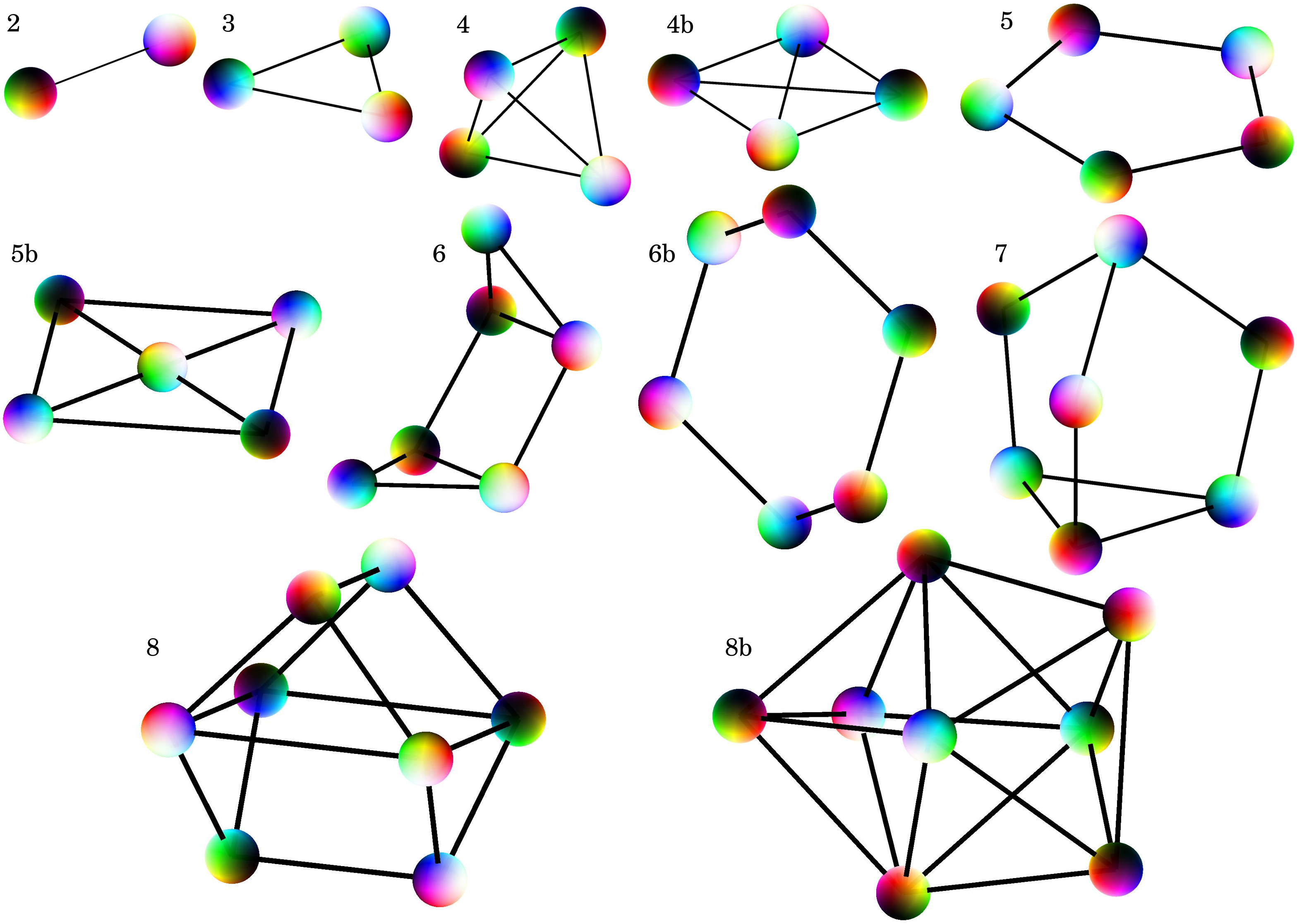
Figure 1: Geometric configurations for stable and metastable nuclei up to $B=8$. The stable (energetically favorable) configurations are labeled with the baryon number $B$ and the metastable states have an added suffix in form of a Latin letter; the further in the alphabet the higher the energy. Bonds are shown for short enough distances between the nuclei as black solid lines. The color scheme is described in the text.

In Fig. 1 we present the numerical results for classical composite nuclei, stable and meta-stable, up to baryon number $B=8$. The stable configurations (ground states) are labeled with their corresponding baryon number $B$, while metastable states have a Latin letter added to the label. With increasing letter in the alphabet, the higher is the energy. This bond between two nuclei symbolizes the 2-body potential, which is used to find these configurations and the bond is displayed only for distances shorter than $1.5R_{0}$ with $R_{0}$ being the optimal distance of two nucleons in deuterium ($B=2$) for $m_{\pi}=0.142$. The color scheme utilized is a map from the unit 2-sphere to the Runge’s color sphere, which is defined by white at the north pole, black at the south pole and the hue of the colors around the equator, going through red, yellow, green, cyan, blue, and magenta as one goes around the equator. The color scheme illustrates the orientation of the point-like instantons in SU(2) space, with the Runge’s color sphere being the standard orientation corresponding to the unit matrix $B=\mathds{1}_{2}$. All points on the color sphere for a nonstandard orientation of the instanton are then rotated by the rotation matrix $M_{ij}(B)$ of Eq. (3.5).

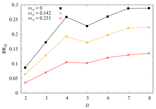
Figure 2: Binding ratios for the stable nuclei (ground states) up to $B=8$, for various values of $m$. In our calibration, the physical pion mass is $m_{\pi}=0.142$ (dimensionless units).

We will now calculate the binding ratios of the $B$ nuclear bound states, defined by

$${\rm BR}_{B}\equiv\frac{BE_{1}-E_{B}}{BE_{1}}\;.$$ (4.2)

The result is shown in Fig. 2. Qualitatively, the bound states show the same spatial/geometrical distributions in the case of a finite pion mass as compared to the massless case, see Fig. 1 and Fig. 5 of Ref. [18]. The optimal distance between two nucleons in the 2-body potential grows with an increasing pion mass and this effectively enlarges all the sizes of the nuclear bound states, but does not affect the orientations of the instantons in SU(2) space. In particular, the optimal distance of the 2-body potential for $m_{\pi}=0$ in dimensionless units is $R_{0}=2.06$ and for $m_{\pi}=0.142$ it is $R_{0}=2.23$. The binding energies and thus the binding ratios, similarly decrease with an increasing pion mass.

On the other hand, the presence of the pion mass removes the long-range force of the potential, so even though the minimum is pushed a bit away in the 2-body potential, the attraction is also shortened somewhat. This has the consequence that some states are different in the massive case, with respect to the massless case. In particular, a metastable state in the $B=5$ sector made of a tetrahedron with a satellite exists in the massless case [18], but has disappeared in the massive case. Similarly, the ground state of the $B=6$ state has changed by moving the leftmost and the topmost nucleon in Fig. 1 closer to the hexagon in the massive case, than in the massless case where it was more compact.

$B$	shape	details	$V_{\rm min}$	BR
2	line	bond length = 2.23	$-0.2197$	$0.0640$
3	equilateral triangle	bond length = 2.23	$-0.6590$	$0.1280$
4	tetrahedron	bond length = 2.23	$-1.3179$	$0.1920$
	square	side bond length = 2.07	$-1.2499$	$0.1821$
5	pentagon	bond length = 2.25	$-1.4721$	$0.1716$
	cross	side bond length = 3.20	$-1.4432$	$0.1682$
6	two triangles forming a bent hexagon, triangles bent the same way	triangle bond lengths = 2.13, 2.28; square bond length = 3.34	$-2.0304$	$0.1972$
	two triangles forming a bent hexagon, triangles bent the opposite way	bond length = 2.17	$-2.0023$	$0.1945$
7	tetrahedron + triangle	bond lengths = 2.12, 2.46, 2.80	$-2.6486$	$0.2205$
8	two triangular prisms sharing the same base, but rotated by 90 degrees	bond lengths = 2.47, 2.70	$-3.0660$	$0.2234$
	pyramid + triangle	bond lengths = 2.96, 3.06, 3.15, 3.21, 3.24	$-2.5576$	$0.1863$

Table 1: Details of stable and metastable multi-instanton solutions for $B=2,\ldots 8$. $V_{\rm min}$ is the potential in dimensionless units and BR is the binding ratio.

The details of the solutions in the massive case with $m_{\pi}=0.142$ are shown in Tab. 1.

5 The deuteron state

The quantum description of the deuteron is obtained by quantization of the collective modes starting from the $B=2$ classical system that we examined in section 3. The procedure has already been described in detail in Ref. [18]: Here we will review the analysis and obtain the binding energy of the deuteron in the system at hand.

A generic field configuration in the two-instanton sector is written by considering only the degrees of freedom that do not change the potential computed in section 3, and fixing all other degrees of freedom to have the potential as attractive as possible. The unfixed degrees of freedom form the zeromode manifold, and can be interpreted in the following way:

• Overall position of the center of mass of the system, that we denote as $x=(x^{1},x^{2},x^{3})$. Due to the gravitational field in the $z$-direction, we do not allow motion along the $z$-axis. Quantizing those degrees of freedom gives the system an overall momentum.

• Isospin of the system: This is represented by an SU(2) matrix called $U$.

• Spin of the system: This is represented by an SU(2) matrix called $E$ and the corresponding SO(3) matrix, $M_{ij}(E)$ is given in Eq. (3.5).

• Parity: We can always switch the two components of the system. As this is a discrete symmetry, it will not induce a momentum. We will indicate parity with a binary variable $P=0,1$.

The relative position and phase are minimized by assuming maximal attraction: This is attained at the separation $R=(R_{0},0,0)$ (with both nuclei centered at the origin of the holographic coordinate) with phase opposition, $B^{\dagger}C=\mathrm{i}\sigma_{3}$. The numerical value of $R_{0}$ is the value at which the potential (3.7) is minimized.

A configuration $\mathcal{A}_{I}$ in the two-instanton sector belongs to the zeromode manifold, if it can be written as

$$\mathcal{A}_{I}(x,z) =UE^{\dagger}A_{I}\left(x-(-)^{P}M(E)\frac{r}{2},z\right)(UE^{\dagger})^{\dagger}$$

$$\mathop{+}U\mathrm{i}\sigma_{3}E^{\dagger}A_{I}\left(x+(-)^{P}M(E)\frac{r}{2},z\right)(U\mathrm{i}\sigma_{3}E^{\dagger})^{\dagger}\;.$$ (5.1)

The kinetic energy is computed by starting from the kinetic energy of two baryons, computed in Ref. [2], and then comparing configuration (5.1) with configuration (3.1) to understand how the collective coordinates are related to the coordinates describing the single baryons. After performing the transformation and freezing the coordinates that are not zeromodes, we obtain the kinetic energy for the zeromode manifold. Since the derivation is the same as in Ref. [18], we will just cite the result here. In terms of the angular left-invariant velocities $\Omega_{i}=-\mathrm{i}\mathop{tr}\nolimits(U^{\dagger}\dot{U}\sigma_{i})$ and $\omega_{i}=-\mathrm{i}\mathop{tr}\nolimits(E^{\dagger}\dot{E}\sigma_{i})$, we have the kinetic energy

$$T=\frac{1}{2}M_{B}\bigg{(}\rho^{2}\omega_{1}^{2}+\left(\rho^{2}+\frac{R_{0}^{2}}{2}\right)\omega_{2}^{2}+\frac{R_{0}^{2}}{2}\omega_{3}^{2}+\rho^{2}\left(\Omega_{1}^{2}+\Omega_{2}^{2}+(\Omega_{3}-\omega_{3})^{2}\right)\bigg{)}\;.$$ (5.2)

The mass $M$ and radius $\rho$ have been computed in subsection 2.2, and the parameter $R_{0}$ is obtained from the potential (3.7) in the attractive channel, by finding the minimum. The Hamiltonian for the deuteron is computed straightforwardly. First, the momenta are defined as

$$L_{1} =M_{B}\rho^{2}\omega_{1}\;, \quad L_{2} =M_{B}\left(\rho^{2}+\frac{R_{0}^{2}}{2}\right)\omega_{2}\;, \quad L_{3} =M_{B}\left(\frac{R_{0}^{2}}{2}+\rho^{2}\right)\omega_{3}-M\rho^{2}\Omega_{3}\;,$$

$$K_{1} =M_{B}\rho^{2}\Omega_{1}\;, \quad K_{2} =M_{B}\rho^{2}\Omega_{2}\;, \quad K_{3} =M_{B}\rho^{2}(\Omega_{3}-\omega_{3})\;.$$ (5.3)

In terms of those momenta, the Hamiltonian reads

$$H=\frac{1}{2M_{B}}\left(X_{ij}L_{i}L_{j}+Y_{ij}K_{i}K_{j}+2Z_{ij}L_{i}K_{j}\right)+V_{\rm min}+2M_{B}\;,$$ (5.4)

where we have included rest mass and defined the inertia tensors $X,Y,Z$ as

$$X \equiv\left(\begin{array}[]{ccc}\frac{1}{\rho^{2}}&0&0\\ 0&\frac{2}{2\rho^{2}+R_{0}^{2}}&0\\ 0&0&\frac{2}{R^{2}_{0}}\\ \end{array}\right),$$ (5.8)

$$\qquad Y \equiv\left(\begin{array}[]{ccc}\frac{1}{\rho^{2}}&0&0\\ 0&\frac{1}{\rho^{2}}&0\\ 0&0&\frac{2}{R_{0}^{2}}+\frac{1}{\rho^{2}}\\ \end{array}\right),$$ (5.12)

$$Z \equiv\left(\begin{array}[]{ccc}0&0&0\\ 0&0&0\\ 0&0&\frac{2}{R_{0}^{2}}\\ \end{array}\right).$$ (5.16)

Quantum states are expressed as

$$\ket{\psi}=\ket{k,k_{3},i_{3},l,l_{3},j_{3}},$$ (5.17)

where $k$ and $l$ are eigenvalues for $K^{2}$ and $L^{2}$, of values $\frac{k}{2}(\frac{k}{2}+1)$ and $\frac{l}{2}(\frac{l}{2}+1)$, respectively, $k_{3}$ and $l_{3}$ are eigenvalues for $K_{3}$ and $L_{3}$, and $i_{3}$ and $j_{3}$ are eigenvalues for the right-invariant momenta $I_{3}$ and $J_{3}$, that commute with the (left-invariant) momenta $K_{3}$ and $L_{3}$ and have the properties $I^{2}=K^{2}$ and $L^{2}=J^{2}$. The right-invariant momenta can be obtained from the left-invariant momenta as $J_{i}=-M(E)_{ij}L_{j}$ and $I_{i}=-M(U)_{ij}K_{j}$ (where $E$ and $U$ are promoted to position operators).

Due to the fact that the configuration space has discrete symmetries (as an example, multiplying $U$ and $E$ by $\mathrm{i}\sigma_{1}$ on the right leaves the configuration invariant) we have to impose Finkelstein-Rubenstein constraints. The analysis in Ref. [18] is still valid: The only states that are compatible with the quantization of the single baryons as fermions and that include the constraints are

$$\ket{D} =\ket{0,0,0,1,0,j_{3}},\qquad\ket{I_{0}}=\ket{1,0,i_{3},0,0,0},$$

$$\ket{I_{1}} =\frac{1}{\sqrt{2}}\left(\ket{1,1,i_{3},0,0,0}+\ket{1,-1,i_{3},0,0,0}\right).$$ (5.18)

Of those states, $\ket{D}$ is the only one having the quantum numbers of the deuteron (isospin $0$ and spin $1$). The energies of the states are computed by acting on them with the Hamiltonian: the final result is

$$H\ket{D} =\left(\frac{1}{2\rho^{2}M_{B}}\left(1+\frac{1}{1+\frac{R_{0}^{2}}{2\rho^{2}}}\right)+2M_{B}+V_{\rm min}\right)\ket{D}=E_{D}\ket{D}\;,$$

$$H\ket{I_{0}} =\left(\frac{1}{\rho^{2}M_{B}}+2M_{B}+V_{\rm min}\right)\ket{I_{0}}=E_{I_{0}}\ket{I_{0}}\;,$$

$$H\ket{I_{1}} =\left(\frac{1}{\rho^{2}M_{B}}\left(1+\frac{\rho^{2}}{R_{0}^{2}}\right)+2M_{B}+V_{\rm min}\right)\ket{I_{1}}=E_{I_{1}}\ket{I_{1}}\;.$$ (5.19)

It is evident that $E_{D}$ is always the smallest energy of the three ones above, so the deuteron state is effectively the ground state of the system. Although the result is identical to the result in Ref. [18] in form, we emphasize that in this setting the values of $M_{B},\rho,V_{\rm min}$ and $R_{0}$ are different, so the final numerical result will be different.

With $E_{D}$ obtained from the first line of (5.19), the most relevant quantity we can compute is the binding energy $E_{D}-2M_{B}$. Various parameters are needed to obtain this value. The new parameters $R_{0}$ and $V_{\rm min}$ are not free, but they are fixed by looking for the minimum of the classical potential (3.7) in the attractive channel ($B^{\dagger}C=\sigma_{3},r=(R_{0},0,0),\rho_{i}=\rho,Z_{i}=0$). In the massive model, we have found $R_{0}=2.23$ and $V_{\rm min}=-0.220$ by including $40$ massive mesons in the potential computation. Furthermore, the instanton size can be computed from Eq. (2.29), obtaining a value of $\rho=2.307$. We can combine these parameters to obtain the binding energy. The classical binding energy in MeV is given by $-V_{\rm min}=208.5$ MeV, and the rotational corrections have a small influence on this value: the quantum binding energy is given by $E_{D}-2M_{B}=208.4$ MeV. This is to be compared against a binding energy of $2.224$ MeV found in experiments. As in our previous work, the binding energy is two orders of magnitude larger than the expected binding energy. The pion mass improves the prediction, as the binding energy of the massless model is $275.5$ MeV. A study of the $\frac{1}{N_{c}}$ and $\frac{1}{\Lambda}$ corrections is required to understand if the prediction for the binding energy can be improved, as the parameters $N_{c}$ and $\Lambda$ are not that large.

6 An infinite lattice of baryons

The attractive channel of the potential between two nucleons is obtained by employing a relative rotation between their SU(2) orientations: The iso-rotation must act by an angle $\pi$ with an axis orthogonal to the relative position vector. Using the axis-angle notation, the matrix $M_{ij}(B^{\dagger}C)$ that describes the relative orientation is given by

$$M_{ij}(\hat{\mathbf{u}},\alpha)=\delta_{ij}\cos\alpha+\left(1-\cos\alpha\right)\hat{u}_{i}\hat{u}_{j}+\epsilon_{ijk}\hat{u}_{k}\sin\alpha\;.$$ (6.1)

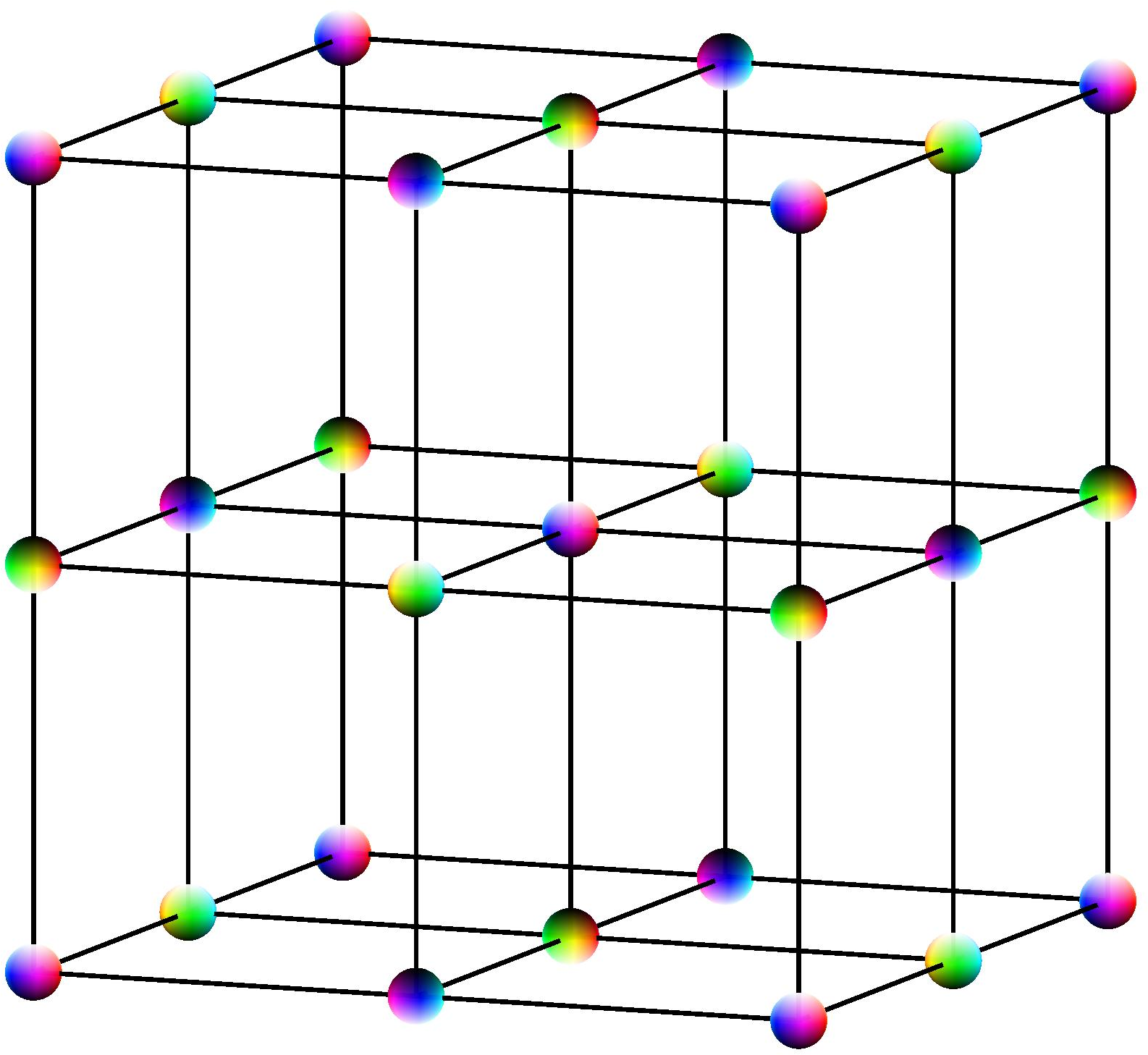
Figure 3: The fundamental cell of the infinite lattice. Careful inspection of the figure reveals that every pair of nucleons, connected with a solid black line, face each other with a matching color, representing the attractive channel described in the text.

It is possible to arrange nucleons in a cubic lattice in such a way that the interaction between all nearest neighbors is in the attractive channel, see fig. 3. The Ansatz for the lattice we are using is equal to that of Ref. [34]. The relation between the instanton lattice studied here and the Skyrmion lattice of Ref. [34] is given by the holonomy of the instanton gauge field [35]. We make the following choices: The relative iso-orientation $B^{\dagger}C$ between every soliton and its nearest neighbors is given by

• $\pm\mathrm{i}\sigma^{2}$ for $\mathbf{r}=(\pm R,0,0)$, corresponding to $\alpha=\pi,\hat{\mathbf{u}}=\hat{x}_{2}$,

• $\pm\mathrm{i}\sigma^{3}$ for $\mathbf{r}=(0,\pm R,0)$, corresponding to $\alpha=\pi,\hat{\mathbf{u}}=\hat{x}_{3}$,

• $\pm\mathrm{i}\sigma^{1}$ for $\mathbf{r}=(0,0,\pm R)$, corresponding to $\alpha=\pi,\hat{\mathbf{u}}=\hat{x}_{1}$.

This choice for the nearest neighbors fixes completely the lattice in a self-consistent way (since $\sigma^{1}\sigma^{2}=\mathrm{i}\sigma^{3}$), so it is now possible to compute the energy density associated to it.

Before moving to the computation, let us make some useful considerations: The relative orientation enters the potential formula via the combination $M_{ij}P_{ij}(\mathbf{r},k)$, which reads

$$M_{ij}(\hat{\mathbf{u}},\alpha)P_{ij}(\mathbf{r},k) =\bigg{(}1+\cos\alpha-\left(1-\cos\alpha\right)\frac{(\hat{\mathbf{u}}\cdot\mathbf{r})^{2}}{r^{2}}\bigg{)}(kr)^{2}$$

$$\phantom{=\ }-(1-\cos\alpha)\left(3\frac{(\hat{\mathbf{u}}\cdot\mathbf{r})^{2}}{r^{2}}-1\right)\left(rk+1\right)\;,\qquad r\equiv\sqrt{\mathbf{r}\cdot\mathbf{r}}\;,$$ (6.2)

so that we have two classes of iso-orientations: $\alpha=0$ and $\alpha=\pi$:

$$M_{ij}(\hat{\mathbf{u}},0)P_{ij}(\mathbf{r},k) =2(rk)^{2}$$

$$M_{ij}(\hat{\mathbf{u}},\pi)P_{ij}(\mathbf{r},k) =2\frac{(\hat{\mathbf{u}}\cdot\mathbf{r})^{2}}{r^{2}}\left[-3(rk+1)-(rk)^{2}\right]+2(rk+1)\;.$$ (6.3)

To compute the full energy density it is sufficient to evaluate the potential between a single chosen nucleon and all the others: Then translational symmetry ensures that the full energy is given by multiplying this contribution by the number of nucleons (which is infinite) with a factor of one half to avoid double counting. The nucleon number can then be traded for the number of cells, as a function of the lattice volume $V_{L}$, so the full energy will be computed as

$$E=\frac{1}{2}\sum_{p}\sum_{p^{\prime}\neq p}V(\mathbf{r}_{pp^{\prime}},B_{p}^{\dagger}C_{p^{\prime}})=\frac{1}{2}\frac{V_{L}}{R^{3}}\sum_{p^{\prime}\neq p}V(\mathbf{r}_{pp^{\prime}},B_{p}^{\dagger}C_{p^{\prime}})\;,\qquad\mathbf{r}_{pp^{\prime}}\equiv\mathbf{r}_{p^{\prime}}-\mathbf{r}_{p}\;,$$ (6.4)

with $p$ indicating a lattice site.

To make the calculation more straightforward, we choose our reference frame in such a way that $\mathbf{r}_{p}=(0,0,0)$ and $B_{p}=\mathds{1}$, so we are left with the following formula for the energy density:

$$\frac{E}{V_{L}}=\frac{1}{2R^{3}}\sum_{p^{\prime}}V(\mathbf{r}_{p^{\prime}},C_{p^{\prime}})=\frac{1}{2R^{3}}\sum_{p^{\prime}}V(\mathbf{r}_{p^{\prime}},\alpha_{p^{\prime}},\hat{\mathbf{u}}_{p^{\prime}})\;,$$ (6.5)

where $p^{\prime}$ runs over all lattice sites with the exception of $(0,0,0)$. The lattice sites are uniquely parametrized as

$$\mathbf{r}=R(n_{1},n_{2},n_{3})\;,\qquad n_{i}\in\mathbb{Z}\;.$$ (6.6)

The position $\mathbf{r}$ not only enters the expression of $M_{ij}P_{ij}$, but it also determines whether $\alpha=0$ or $\alpha=\pi$: We must therefore be careful and classify iso-orientations with respect to $(n_{1},n_{2},n_{3})$. There are four possible scenarios, depending on how many even or odd instances of $n_{i}$ are present in the position vector:

• all $n_{i}$ are EVEN $\Rightarrow C_{p^{\prime}}=\mathds{1}$,

• all $n_{i}$ are ODD $\Rightarrow C_{p^{\prime}}=\mathds{1}$,

• one $n_{i}$ is EVEN $\Rightarrow C_{p^{\prime}}=\pm\mathrm{i}\sigma^{j}$,

• one $n_{i}$ is ODD $\Rightarrow C_{p^{\prime}}=\pm\mathrm{i}\sigma^{j}$,

where in the last two lines $\sigma^{j}$ indicates a rotation around the axis determined by our rule for the rotation of nearest neighbors (that is, $j=2$ for $i=1$, $j=3$ for $i=2$ and $j=1$ for $i=3$). For example, a nucleon sitting at $R(2b_{1}-1,2b_{2},2b_{3})$ with $b_{i}\in\mathbb{Z}$ will have an orientation of $\pm\mathrm{i}\sigma^{2}$, i.e. the same as a nucleon sitting at $R(2b_{1},2b_{2}-1,2b_{3}-1)$. The last two scenarios fall into the class of $\alpha=\pi$, and the axis of rotation enters Eq. (6.2) only via $(\hat{\mathbf{u}}\cdot\mathbf{r})$, which selects the component of $\mathbf{r}$ along the axis $\hat{\mathbf{u}}$. But since $\hat{\mathbf{u}}$ is a unit vector corresponding to one of the coordinate axes, this simply selects the $j$-th component $Rn_{j}$.

Now we will compute the contributions to the energy density: Let us start with the first two possibilities in the classification, corresponding to all even or all odd $n_{i}$, for which we obtain

$$\frac{E_{1,2}}{V_{L}}=\frac{4\pi N_{c}}{2R^{3}\Lambda}\!\sum_{b_{1},b_{2},b_{3}}\!\!\left[\sum_{n=1}^{\infty}\left(\frac{1}{c_{2n-1}}\frac{e^{-k_{2n-1}r}}{r}+\frac{12k_{2n-1}^{2}}{5c_{2n-1}}\frac{e^{-k_{2n-1}r}}{r}-\frac{12k_{2n}^{2}}{5d_{2n}}\frac{e^{-k_{2n}r}}{r}\right)-\frac{12k_{0}^{2}}{5\pi}\frac{e^{-k_{0}r}}{r}\right]\!,$$ (6.7)

with $r^{2}=4R^{2}(b_{1}^{2}+b_{2}^{2}+b_{3}^{2})$ for the even case ($E_{1}$) and $r^{2}=R^{2}[(2b_{1}-1)^{2}+(2b_{2}-1)^{2}+(2b_{3}-1)^{2}]$ for the odd case ($E_{2}$). We now turn to the more difficult scenarios: We start by considering $\mathbf{r}=(2b_{1}-1,2b_{2},2b_{3})R$ with $b_{i}\in\mathbb{Z}$. In this case the energy density becomes

$$\frac{E_{3}^{(1)}}{V_{L}}=\frac{E_{3,4}^{p}(4b_{2}^{2})}{V_{L}}\;,$$ (6.8)

where we have defined

$$\frac{E_{3,4}^{p}(b)}{V_{L}}\equiv \frac{4\pi N_{c}}{2R^{3}\Lambda}\sum_{b_{1},b_{2},b_{3}}\left[\sum_{n=1}^{\infty}\left[\frac{1}{c_{2n-1}}\frac{e^{-k_{2n-1}r}}{r}\right.\right.$$

$$\left.\left.+\frac{6}{5}\frac{2}{c_{2n-1}}\left(\frac{b}{r^{2}}\left(-3(rk_{2n-1}+1)-(rk_{2n-1})^{2}\right)+\left(rk_{2n-1}+1\right)\right)\frac{e^{-k_{2n-1}r}}{r^{3}}\right.\right.$$

$$\left.\left.-\frac{6}{5}\frac{2}{d_{2n}}\left(\frac{b}{r^{2}}\left(-3(rk_{2n}+1)-(rk_{2n})^{2}\right)+\left(rk_{2n}+1\right)\right)\frac{e^{-k_{2n}r}}{r^{3}}\right]\right.$$

$$-\frac{12}{5\pi}\frac{e^{-k_{0}r}}{r^{3}}\left(1+rk_{0}-\frac{bR^{2}}{r^{2}}\left(3+3k_{0}r+k_{0}^{2}r^{2}\right)\right)\Bigg{]}\;,$$ (6.9)

with $r^{2}=R^{2}[(2b_{1}-1)^{2}+4b_{2}^{2}+4b_{3}^{2}]$. We can see that the other terms labeled by $E^{(2,3)}_{3}$ will have the same form except for the substitution of every instance of $b_{2}$ with respectively $b_{3},b_{1}$: Since the sum runs over all three parameters, then each of these terms will give contribution equal to the result

$$\frac{E_{3}}{V_{L}}=3\frac{E_{3}^{(1)}}{V_{L}}\;.$$ (6.10)

We are thus only left with the terms of the case in which one coordinate is an even multiple of the lattice spacing, while the others are odd. As before we begin by analyzing the situation in which this coordinate is $r_{1}$, so that $\mathbf{r}=R(2b_{1},2b_{2}-1,2b_{3}-1)$: The result is just as the previous one, with the exception that the projection on the $j$-th component of $\mathbf{r}$ due to the rotation axis will now pick up an odd value instead of an even one, so that

$$\frac{E_{4}^{(1)}}{V_{L}}=\frac{E_{3,4}^{p}((2b_{2}-1)^{2})}{V_{L}}\;.$$ (6.11)

and $r$ is now given by $r^{2}=R^{2}[4b_{1}^{2}+(2b_{2}-1)^{2}+(2b_{3}-1)^{2}]$. Again, as in the previous case, the sum of all three possible combinations with only one even coordinate will just result in a factor of three, so we get

$$\frac{E_{4}}{V_{L}}=3\frac{E_{4}^{(1)}}{V_{L}}\;.$$ (6.12)

The total energy density is then given by the sum of the contributions from all four possibilities in the classification, giving

$$\frac{E_{\rm tot}}{V_{L}}=\frac{1}{V_{L}}\left(E_{1}+E_{2}+E_{3}+E_{4}\right)\;.$$ (6.13)

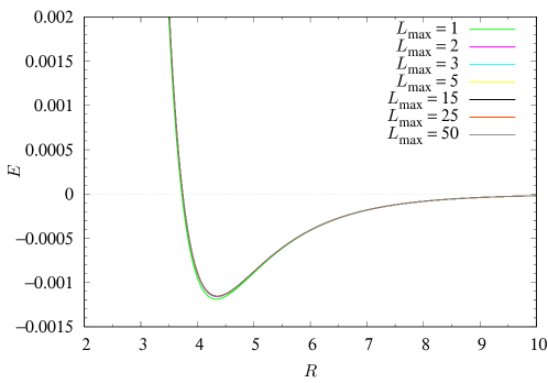
Figure 4: The shape of the potential energy density around its minimum. $L_{\rm max}$ is the cutoff of lattice sites: $|b_{j}|\leq L_{\rm max}$.

The total lattice potential can then be computed numerically and plotted as a function of the lattice spacing $R$: the sum over lattice sites converges with good precision ($\sim 10^{-5}$) for $b_{j}\in[-L_{\rm max},L_{\rm max}]$ with $L_{\rm max}=15$, $\forall$ $j=1,2,3$. Notice that the cutoff in terms of lattice sides is $2L_{\rm max}$ in each direction (i.e. both in the $x+$ direction and in the $x-$ direction) and the factor of two is due to $b_{j}$ being an integer parametrizing even or odd $n_{j}$’s. The resulting potential density has a shallow minimum at $R=4.86$ (see Fig. 4).

It is not straightforwardly clear that the quadruple sum in Eqs. (6.7) and (6.9) are convergent in the limit of $L_{\rm max}\to\infty$, i.e. in the limit of summing over all lattice sites $b_{j}$ and all massive vectors $n$ (being the index of $k_{n}$). The convergence of the quadruple sum would prove that the density in the given form is finite. We give a mathematical proof of the convergence of each term in the sums separately in appendix A.

6.1 Hadronic phase transition

We will now use the baryon lattice to study the presence of a hadronic phase transition: To do so we need to compute the free energy of the configuration and look for a critical density at which it becomes negative.

We can do this without relying on holography, simply by calculating the Legendre transform of the energy density. First of all, we recover the total energy density from the interaction potential density by adding the mass density terms: the cubic lattice cell has unit net baryon number, so the mass density as a function of the lattice spacing $R$ is simply

$$\mathcal{M}(R)=M_{B}R^{-3}\;,$$ (6.14)

with $M_{B}$ given by Eq. (2.30).

The chemical potential is defined as the derivative of the energy density with respect to the baryon number density (which we can trade for a derivative with respect to $R$, since the baryon number density is $d_{B}=R^{-3}$):

$$\mu=-\frac{R^{4}}{3}\frac{\partial}{\partial R}\left(EV_{L}^{-1}+M_{B}R^{-3}\right),$$ (6.15)

with $EV_{L}^{-1}$ given by Eq. (6.13).

We want to compare the free energy density of the infinite lattice of baryons constructed above, with that of the vacuum: the embedding of the flavor branes is the same for both phases, so we neglect its contribution to both phases, effectively setting to zero the free energy of the vacuum. All we need to compute is then the change in free energy due to the presence of baryons: the lattice configuration will become favored over the vacuum (that is, a purely mesonic phase) for negative values of this free energy. The free energy density $F$ is then obtained from the energy density as:

$$F =EV_{L}^{-1}+\mathcal{M}(R)-\mu R^{-3}$$

$$=EV_{L}^{-1}+\frac{R}{3}\frac{\partial}{\partial R}EV_{L}^{-1}\;.$$ (6.16)

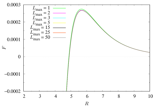
Figure 5: The free energy density as a function of the lattice spacing $R$. As the density increases (i.e. $R$ decreases), the free energy becomes negative, signaling a phase transition. $L_{\rm max}$ is the cutoff of lattice sites: $|b_{j}|\leq L_{\rm max}$.

In Fig. 5, we plot the free energy density as a function of $R$, showing that it becomes negative at a finite density, signaling the presence of a first-order hadronic phase transition. Note that with this analysis we cannot conclude that the favored of all phases is indeed given by this lattice of baryons, but only that it is favored over the vacuum. Different configurations of baryonic matter can potentially give rise to even lower free energies, and become favored over this particular lattice.

7 Conclusion

In this paper, we have included the quark mass term using the Aharony-Kutasov action in our solitonic approach to holographic nuclear physics. We work in the limit $\Lambda\to\infty$, where the size of the instantons is much smaller than the typical separation distance between nuclei in a nuclear bound state. This allows us to calculate multi-instanton solutions by gluing together two overlapping instantons in the linear regime; in particular, we compute the 2-body potential which now has acquired a mass term for the pions. This induction of the pion mass from the quark mass term is in line with the GMOR relation. Using numerical methods we find nuclear bound states – stable and metastable – with baryon numbers $B=2$ through $B=8$.

We find that the main difference by having massive pions in the 2-body potential is that the nuclear bound states grow slightly in size and correspondingly reduce their binding energy. A similar effect applies also to the deuteron bound state and to the other light nuclei.

Using the 2-body potential, we consider the case of an infinite crystal of nucleons in a cubic lattice with each nucleon oriented in SU(2) space so as to put it in the attractive channel with respect to nearest neighbors. We calculate the potential energy density, prove in appendix A that it is finite, and finally use it to calculate the free energy. The free energy becomes negative at a critical lattice spacing $R_{\rm crit}\sim 4.9$, which signals a hadronic phase transition of first order. The presence of the hadronic phase transition was also studied in the same model in Refs. [36, 37, 38, 39]: The difference with our approach lies both in the description of the solitons and in the setup of the flavor branes. In the cited works the branes’ position at infinity are taken to be close enough to allow the use of the deconfined geometry up to arbitrarily low temperatures, thus being far from the antipodal branes’ regime: the baryonic matter is described with various levels of accuracy, starting from exactly pointlike instantons up to an infinite lattice of finite size instantons interacting with the nearest neighbors via the ADHM construction. We work instead with antipodal branes at zero temperature, using the confined geometry, and we employ the flat space instanton approximation, then take into account every single interaction (up to a cutoff in lattice size) with every soliton seeing each other’s core as pointlike. The presence of the first order phase transition remains a feature of the model in both regimes, and is becoming of second order if interactions between instantons are ignored [36].

The work carried out in this paper has been done in the large $\Lambda$ and large ${N_{\rm c}}$ limit, which is of course none other than approximations to real world physics, as neither parameters take (that) large phenomenological values (i.e. $\Lambda_{\rm SS}=1.569$ and ${N_{\rm c}}=3$). It would be interesting to calculate, for instance, the leading $\Lambda^{-1}$ correction to the 2-body potential and see if this could improve some phenomenological properties of our results, for example the large binding energies. Of course, this would turn the problem into a nonlinear one and make it severely more difficult than the one we have solved here.

The large-$N_{c}$ approximation may be a poor approximation for the physics at finite density, such as the baryon crystal studied in the last part of this paper, and subleading $1/N_{c}$ corrections may alter our results and even the presence or absence of phase transitions, see e.g. Refs. [40, 41]. This can be attributed to the fact that the number of nearest neighbors in a cubic lattice is 6 and $N_{c}=3$ in Nature, but in the large-$N_{c}$ limit, the number of colors is much larger than the number of nearest neighbors – this has consequences for, e.g. the van Der Waals forces, etc.

Appendix A Proof of convergence

We now give a proof that the energy density for the infinite lattice of baryons (6.13) is a convergent sum, by giving an upper bound for each term. In this appendix, $m$ denotes a parameter comparable to the pion mass and should not be confused with the quark mass in the main text.

Lemma 1

The following quadruple sum obeys the inequality

$$\sum_{\begin{subarray}{c}n=0\\ b_{1},b_{2},b_{3}=-\infty\\ (b_{1},b_{2},b_{3})\neq 0\end{subarray}}^{\infty}\frac{e^{-k_{n}R\sqrt{b_{1}^{2}+b_{2}^{2}+b_{3}^{2}}}}{c_{n}R^{p}(b_{1}^{2}+b_{2}^{2}+b_{3}^{2})^{\frac{p}{2}}}\leq\frac{\mathcal{A}_{p}(m,R)\mathcal{G}{\left(\frac{\eta R}{2}\right)}+\mathcal{B}_{p}(m,R)\mathcal{G}{\left(\frac{3\eta R}{2}\right)}}{\min(\{c_{n}\})}\;,$$ (A.1)

provided $k_{n}$ obeys $k_{n}\geq m+\eta n$ with $m>0$, $\eta>0$ positive constants, and $p\in\mathbb{Z}_{>0}$.

Proof: Using $\sqrt{A^{2}+B^{2}+C^{2}}\geq\frac{|A|+|B|+|C|}{2}$, we have for the triple sum

$$\sum_{\begin{subarray}{c}b_{1},b_{2},b_{3}=-\infty\\ (b_{1},b_{2},b_{3})\neq(0,0,0)\end{subarray}}^{\infty}e^{-k\sqrt{b_{1}^{2}+b_{2}^{2}+b_{3}^{2}}}\leq\sum_{\begin{subarray}{c}b_{1},b_{2},b_{3}=-\infty\\ (b_{1},b_{2},b_{3})\neq(0,0,0)\end{subarray}}^{\infty}e^{-\frac{k}{2}|b_{1}|}e^{-\frac{k}{2}|b_{2}|}e^{-\frac{k}{2}|b_{3}|}=\frac{3e^{\frac{k}{4}}+e^{-\frac{3k}{4}}}{4\sinh^{3}{\left(\frac{k}{4}\right)}}\;.$$ (A.2)

At this point we include the fourth sum over $n$:

$$\sum_{\begin{subarray}{c}n=0\\ b_{1},b_{2},b_{3}=-\infty\\ (b_{1},b_{2},b_{3})\neq(0,0,0)\end{subarray}}^{\infty}e^{-k_{n}R\sqrt{b_{1}^{2}+b_{2}^{2}+b_{3}^{2}}}\leq\sum_{\begin{subarray}{c}n=0\\ b_{1},b_{2},b_{3}=-\infty\\ (b_{1},b_{2},b_{3})\neq(0,0,0)\end{subarray}}^{\infty}e^{-(m+\eta n)R\sqrt{b_{1}^{2}+b_{2}^{2}+b_{3}^{2}}}$$

$$\ \ \leq\sum_{\begin{subarray}{c}n=0\\ b_{1},b_{2},b_{3}=-\infty\\ (b_{1},b_{2},b_{3})\neq(0,0,0)\end{subarray}}^{\infty}e^{-\frac{1}{2}(m+\eta n)R(|b_{1}|+|b_{2}|+|b_{3}|)}=\sum_{n=0}^{\infty}\frac{3e^{\frac{1}{4}(m+\eta n)R}+e^{-\frac{3}{4}(m+\eta n)R}}{4\sinh^{3}{\left(\frac{1}{4}(m+\eta n)R\right)}}$$

$$\ \ \leq\frac{3e^{\frac{mR}{4}}\mathcal{G}{\left(\frac{\eta R}{2}\right)}+e^{-\frac{3mR}{4}}\mathcal{G}{\left(\frac{3\eta R}{2}\right)}}{4\sinh^{3}{\left(\frac{mR}{4}\right)}}\;,$$ (A.3)

where we have used that

$$\sinh{\left(\frac{mR}{4}+\frac{\eta nR}{4}\right)}\geq\sinh{\left(\frac{mR}{4}\right)}e^{\frac{\eta nR}{4}}\;,\quad m>0\;,\quad R>0\;,\quad n\in\mathbb{Z}_{\geq 0}\;,$$ (A.4)

and we have defined

$$\mathcal{G}(x)\equiv\frac{1}{1-e^{-x}}\;,\qquad x>0\;.$$ (A.5)

Next we need the Yukawa-like sum

$$\sum_{\begin{subarray}{c}b_{1},b_{2},b_{3}=-\infty\\ (b_{1},b_{2},b_{3})\neq(0,0,0)\end{subarray}}^{\infty}\frac{e^{-kR\sqrt{b_{1}^{2}+b_{2}^{2}+b_{3}^{2}}}}{R^{p}(b_{1}^{2}+b_{2}^{2}+b_{3}^{2})^{\frac{p}{2}}} =\int_{k}^{\infty}\mathrm{d}{m_{1}}\cdots\int_{m_{p-1}}^{\infty}\mathrm{d}{m_{p}}\sum_{\begin{subarray}{c}b_{1},b_{2},b_{3}=-\infty\\ (b_{1},b_{2},b_{3})\neq(0,0,0)\end{subarray}}^{\infty}e^{-m_{p}R\sqrt{b_{1}^{2}+b_{2}^{2}+b_{3}^{2}}}$$

$$\leq\int_{k}^{\infty}\mathrm{d}{m_{1}}\cdots\int_{m_{p-1}}^{\infty}\mathrm{d}{m_{p}}\left[\coth^{3}{\left(\frac{m_{p}R}{4}\right)}-1\right],$$ (A.6)

for $p\in\mathbb{Z}_{>0}$ and $k>0$. Combining this result with the fourth sum of Eq. (A.3), we obtain the following result

$$\sum_{\begin{subarray}{c}n=0\\ b_{1},b_{2},b_{3}=-\infty\\ (b_{1},b_{2},b_{3})\neq(0,0,0)\end{subarray}}^{\infty}\frac{e^{-k_{n}R\sqrt{b_{1}^{2}+b_{2}^{2}+b_{3}^{2}}}}{R^{p}(b_{1}^{2}+b_{2}^{2}+b_{3}^{2})^{\frac{p}{2}}}\leq\sum_{\begin{subarray}{c}n=0\\ b_{1},b_{2},b_{3}=-\infty\\ (b_{1},b_{2},b_{3})\neq(0,0,0)\end{subarray}}^{\infty}\frac{e^{-(m+\eta n)R\sqrt{b_{1}^{2}+b_{2}^{2}+b_{3}^{2}}}}{R^{p}(b_{1}^{2}+b_{2}^{2}+b_{3}^{2})^{\frac{p}{2}}}$$

$$\ \ =\int_{m}^{\infty}\mathrm{d}{m_{1}}\cdots\int_{m_{p-1}}^{\infty}\mathrm{d}{m_{p}}\sum_{\begin{subarray}{c}n=0\\ b_{1},b_{2},b_{3}=-\infty\\ (b_{1},b_{2},b_{3})\neq(0,0,0)\end{subarray}}^{\infty}e^{-(m_{p}+\eta n)R\sqrt{b_{1}^{2}+b_{2}^{2}+b_{3}^{2}}}$$

$$\ \ \leq\int_{m}^{\infty}\mathrm{d}{m_{1}}\cdots\int_{m_{p-1}}^{\infty}\mathrm{d}{m_{p}}\frac{3e^{\frac{mR}{4}}\mathcal{G}{\left(\frac{\eta R}{2}\right)}+e^{-\frac{3mR}{4}}\mathcal{G}{\left(\frac{3\eta R}{2}\right)}}{4\sinh^{3}{\left(\frac{mR}{4}\right)}}$$

$$\ \ =\mathcal{A}_{p}(m,R)\mathcal{G}{\left(\frac{\eta R}{2}\right)}+\mathcal{B}_{p}(m,R)\mathcal{G}{\left(\frac{3\eta R}{2}\right)}\;,$$ (A.7)

with the functions

$$\mathcal{A}_{1}(m,R)=\frac{6\big{(}1-2e^{\frac{mR}{2}}\big{)}}{R\big{(}e^{\frac{mR}{2}}-1\big{)}^{2}},\quad\mathcal{B}_{1}(m,R)=\frac{2}{R}\left[mR+\frac{3-2e^{\frac{mR}{2}}}{\big{(}e^{\frac{mR}{2}}-1\big{)}^{2}}-2\log\big{(}e^{\frac{mR}{2}}-1\big{)}\right],$$

$$\mathcal{A}_{2}(m,R)=\frac{6}{R^{2}}\left[mR+\frac{2}{e^{\frac{mR}{2}}-1}-2\log\big{(}e^{\frac{mR}{2}}-1\big{)}\right],$$

$$\mathcal{B}_{2}(m,R)=\frac{2}{R^{2}}\left[-3mR+\frac{2}{e^{\frac{mR}{2}}-1}+6\log\big{(}e^{\frac{mR}{2}}-1\big{)}+4\mathrm{Li}_{2}\big{(}e^{-\frac{mR}{2}}\big{)}\right],$$

$$\mathcal{A}_{3}(m,R)=\frac{24}{R^{3}}\left[\frac{mR}{2}-\log\big{(}e^{\frac{mR}{2}}-1\big{)}+\mathrm{Li}_{2}\big{(}e^{-\frac{mR}{2}}\big{)}\right],$$

$$\mathcal{B}_{3}(m,R)=\frac{8}{R^{3}}\bigg{[}\frac{mR}{2}-\log\big{(}e^{\frac{mR}{2}}-1\big{)}-3\mathrm{Li}_{2}\big{(}e^{-\frac{mR}{2}}\big{)}+2\mathrm{Li}_{3}\big{(}e^{-\frac{mR}{2}}\big{)}\bigg{]}\;,$$ (A.8)

where $\mathrm{Li}_{2}$ is the dilogarithm or Spence function and $\mathrm{Li}_{3}$ is the trilogarithm. Finally, we can write

$$\sum_{\begin{subarray}{c}n=0\\ b_{1},b_{2},b_{3}=-\infty\\ (b_{1},b_{2},b_{3})\neq(0,0,0)\end{subarray}}^{\infty}\frac{e^{-k_{n}R\sqrt{b_{1}^{2}+b_{2}^{2}+b_{3}^{2}}}}{c_{n}R^{p}(b_{1}^{2}+b_{2}^{2}+b_{3}^{2})^{\frac{p}{2}}} \leq\sum_{\begin{subarray}{c}n=0\\ b_{1},b_{2},b_{3}=-\infty\\ (b_{1},b_{2},b_{3})\neq(0,0,0)\end{subarray}}^{\infty}\frac{e^{-k_{n}R\sqrt{b_{1}^{2}+b_{2}^{2}+b_{3}^{2}}}}{\min(\{c_{n}\})R^{p}(b_{1}^{2}+b_{2}^{2}+b_{3}^{2})^{\frac{p}{2}}}$$

$$=\frac{\mathcal{A}_{p}(m,R)\mathcal{G}{\left(\frac{\eta R}{2}\right)}+\mathcal{B}_{p}(m,R)\mathcal{G}{\left(\frac{3\eta R}{2}\right)}}{\min(\{c_{n}\})}\;.$$ (A.9)

$\square$

Lemma 2

The following quadruple sum obeys the inequality

$$\sum_{\begin{subarray}{c}n=0\\ b_{1},b_{2},b_{3}=-\infty\\ (b_{1},b_{2},b_{3})\neq 0\end{subarray}}^{\infty}\frac{k_{n}e^{-k_{n}R\sqrt{b_{1}^{2}+b_{2}^{2}+b_{3}^{2}}}}{c_{n}R^{p-1}(b_{1}^{2}+b_{2}^{2}+b_{3}^{2})^{\frac{p-1}{2}}} \leq m_{+}\frac{\mathcal{A}_{p-1}(m_{-},R)\mathcal{G}{\left(\frac{\eta_{-}R}{2}\right)}+\mathcal{B}_{p-1}(m_{-},R)\mathcal{G}{\left(\frac{3\eta_{-}R}{2}\right)}}{\min(\{c_{n}\})}$$

$$\phantom{\leq\ }-\frac{\eta_{+}R}{2}\frac{\mathcal{A}_{p}(m_{-},R)\mathcal{G}^{\prime}{\left(\frac{\eta_{-}R}{2}\right)}+\mathcal{B}_{p}(m_{-},R)\mathcal{G}^{\prime}{\left(\frac{3\eta_{-}R}{2}\right)}}{\min(\{c_{n}\})}\;,$$ (A.10)

provided $k_{n}$ obeys $k_{n}\geq m_{-}+\eta_{-}n$ and $k_{n}\leq m_{+}+\eta_{+}n$ with $m_{\pm}>0$, $\eta_{\pm}>0$ positive constants, and $p\in\mathbb{Z}_{>1}$.

Proof: Following the lines of the proof of Lemma 1, we have

$$\sum_{\begin{subarray}{c}n=0\\ b_{1},b_{2},b_{3}=-\infty\\ (b_{1},b_{2},b_{3})\neq 0\end{subarray}}^{\infty}\frac{k_{n}e^{-k_{n}R\sqrt{b_{1}^{2}+b_{2}^{2}+b_{3}^{2}}}}{c_{n}R^{p-1}(b_{1}^{2}+b_{2}^{2}+b_{3}^{2})^{\frac{p-1}{2}}}\leq\sum_{\begin{subarray}{c}n=0\\ b_{1},b_{2},b_{3}=-\infty\\ (b_{1},b_{2},b_{3})\neq 0\end{subarray}}^{\infty}\frac{(m_{+}+\eta_{+}n)e^{-(m_{-}+\eta_{-}n)R\sqrt{b_{1}^{2}+b_{2}^{2}+b_{3}^{2}}}}{c_{n}R^{p-1}(b_{1}^{2}+b_{2}^{2}+b_{3}^{2})^{\frac{p-1}{2}}}$$

$$\ \ \leq\sum_{\begin{subarray}{c}n=0\\ b_{1},b_{2},b_{3}=-\infty\\ (b_{1},b_{2},b_{3})\neq 0\end{subarray}}^{\infty}m_{+}\frac{e^{-(m_{-}+\eta_{-}n)R\sqrt{b_{1}^{2}+b_{2}^{2}+b_{3}^{2}}}}{c_{n}R^{p-1}(b_{1}^{2}+b_{2}^{2}+b_{3}^{2})^{\frac{p-1}{2}}}-\sum_{\begin{subarray}{c}n=0\\ b_{1},b_{2},b_{3}=-\infty\\ (b_{1},b_{2},b_{3})\neq 0\end{subarray}}^{\infty}\eta_{+}\frac{\mathrm{d}}{\mathrm{d}\eta_{-}}{\left(\frac{e^{\left(-(m_{-}+\eta_{-}n)R\sqrt{b_{1}^{2}+b_{2}^{2}+b_{3}^{2}}\right)}}{c_{n}R^{p}(b_{1}^{2}+b_{2}^{2}+b_{3}^{2})^{\frac{p}{2}}}\right)}$$

$$\ \ \leq m_{+}\frac{\mathcal{A}_{p-1}(m_{-},R)\mathcal{G}{\left(\frac{\eta_{-}R}{2}\right)}+\mathcal{B}_{p-1}(m_{-},R)\mathcal{G}{\left(\frac{3\eta_{-}R}{2}\right)}}{\min(\{c_{n}\})}$$

$$\ \ \ \ \ \ -\frac{\eta_{+}R}{2}\frac{\mathcal{A}_{p}(m_{-},R)\mathcal{G}^{\prime}{\left(\frac{\eta_{-}R}{2}\right)}+\mathcal{B}_{p}(m_{-},R)\mathcal{G}^{\prime}{\left(\frac{3\eta_{-}R}{2}\right)}}{\min(\{c_{n}\})}\;,$$ (A.11)

where $k_{n}\geq m_{-}+\eta_{-}n$ and $k_{n}\leq m_{+}+\eta_{+}n$ and the derivative with respect to the argument of $\mathcal{G}$ is

$$\mathcal{G}^{\prime}(x)=-\frac{e^{-x}}{(1-e^{-x})^{2}}\;.$$ (A.12)

$\square$

Lemma 3

The following quadruple sum obeys the inequality

$$\sum_{\begin{subarray}{c}n=0\\ b_{1},b_{2},b_{3}=-\infty\\ (b_{1},b_{2},b_{3})\neq 0\end{subarray}}^{\infty} \frac{k_{n}^{2}e^{-k_{n}R\sqrt{b_{1}^{2}+b_{2}^{2}+b_{3}^{2}}}}{c_{n}R^{p-2}(b_{1}^{2}+b_{2}^{2}+b_{3}^{2})^{\frac{p-2}{2}}}\leq m_{+}^{2}\frac{\mathcal{A}_{p-2}(m_{-},R)\mathcal{G}{\left(\frac{\eta_{-}R}{2}\right)}+\mathcal{B}_{p-2}(m_{-},R)\mathcal{G}{\left(\frac{3\eta_{-}R}{2}\right)}}{\min(\{c_{n}\})}$$

$$-m_{+}\eta_{+}R\frac{\mathcal{A}_{p-1}(m_{-},R)\mathcal{G}^{\prime}{\left(\frac{\eta_{-}R}{2}\right)}+\mathcal{B}_{p-1}(m_{-},R)\mathcal{G}^{\prime}{\left(\frac{3\eta_{-}R}{2}\right)}}{\min(\{c_{n}\})}$$

$$+\frac{\eta_{+}^{2}R^{2}}{4}\frac{\mathcal{A}_{p}(m_{-},R)\mathcal{G}^{\prime\prime}{\left(\frac{\eta_{-}R}{2}\right)}+\mathcal{B}_{p}(m_{-},R)\mathcal{G}^{\prime\prime}{\left(\frac{3\eta_{-}R}{2}\right)}}{\min(\{c_{n}\})}\;,$$ (A.13)

provided $k_{n}$ obeys $k_{n}\geq m_{-}+\eta_{-}n$ and $k_{n}\leq m_{+}+\eta_{+}n$ with $m_{\pm}>0$, $\eta_{\pm}>0$ positive constants, and $p\in\mathbb{Z}_{>2}$.

Proof: Following the lines of the proof of Lemmata 1 and 2, we have

$$\sum_{\begin{subarray}{c}n=0\\ b_{1},b_{2},b_{3}=-\infty\\ (b_{1},b_{2},b_{3})\neq 0\end{subarray}}^{\infty}\frac{k_{n}^{2}e^{-k_{n}R\sqrt{b_{1}^{2}+b_{2}^{2}+b_{3}^{2}}}}{c_{n}R^{p-2}(b_{1}^{2}+b_{2}^{2}+b_{3}^{2})^{\frac{p-2}{2}}}\leq\sum_{\begin{subarray}{c}n=0\\ b_{1},b_{2},b_{3}=-\infty\\ (b_{1},b_{2},b_{3})\neq 0\end{subarray}}^{\infty}\frac{(m_{+}+\eta_{+}n)^{2}e^{-(m_{-}+\eta_{-}n)R\sqrt{b_{1}^{2}+b_{2}^{2}+b_{3}^{2}}}}{c_{n}R^{p-2}(b_{1}^{2}+b_{2}^{2}+b_{3}^{2})^{\frac{p-2}{2}}}$$

$$\ \ \leq\sum_{\begin{subarray}{c}n=0\\ b_{1},b_{2},b_{3}=-\infty\\ (b_{1},b_{2},b_{3})\neq 0\end{subarray}}^{\infty}m_{+}^{2}\frac{e^{-(m_{-}+\eta_{-}n)R\sqrt{b_{1}^{2}+b_{2}^{2}+b_{3}^{2}}}}{c_{n}R^{p-2}(b_{1}^{2}+b_{2}^{2}+b_{3}^{2})^{\frac{p-2}{2}}}$$

$$\phantom{=\ }-\sum_{\begin{subarray}{c}n=0\\ b_{1},b_{2},b_{3}=-\infty\\ (b_{1},b_{2},b_{3})\neq 0\end{subarray}}^{\infty}2m_{+}\eta_{+}\frac{\mathrm{d}}{\mathrm{d}\eta_{-}}{\left(\frac{e^{-(m_{-}+\eta_{-}n)R\sqrt{b_{1}^{2}+b_{2}^{2}+b_{3}^{2}}}}{c_{n}R^{p-1}(b_{1}^{2}+b_{2}^{2}+b_{3}^{2})^{\frac{p-1}{2}}}\right)}$$

$$\phantom{=\ }\ \ \ \ +\sum_{\begin{subarray}{c}n=0\\ b_{1},b_{2},b_{3}=-\infty\\ (b_{1},b_{2},b_{3})\neq 0\end{subarray}}^{\infty}\eta_{+}^{2}\frac{\mathrm{d}^{2}}{\mathrm{d}\eta_{-}^{2}}{\left(\frac{e^{-(m_{-}+\eta_{-}n)R\sqrt{b_{1}^{2}+b_{2}^{2}+b_{3}^{2}}}}{c_{n}R^{p}(b_{1}^{2}+b_{2}^{2}+b_{3}^{2})^{\frac{p}{2}}}\right)}$$

$$\ \ \leq m_{+}^{2}\frac{\mathcal{A}_{p-2}(m_{-},R)\mathcal{G}{\left(\frac{\eta_{-}R}{2}\right)}+\mathcal{B}_{p-2}(m_{-},R)\mathcal{G}{\left(\frac{3\eta_{-}R}{2}\right)}}{\min(\{c_{n}\})}$$

$$\phantom{=\ }\ \ -m_{+}\eta_{+}R\frac{\mathcal{A}_{p-1}(m_{-},R)\mathcal{G}^{\prime}{\left(\frac{\eta_{-}R}{2}\right)}+\mathcal{B}_{p-1}(m_{-},R)\mathcal{G}^{\prime}{\left(\frac{3\eta_{-}R}{2}\right)}}{\min(\{c_{n}\})}$$

$$\phantom{=\ }\ \ +\frac{\eta_{+}^{2}R^{2}}{4}\frac{\mathcal{A}_{p}(m_{-},R)\mathcal{G}^{\prime\prime}{\left(\frac{\eta_{-}R}{2}\right)}+\mathcal{B}_{p}(m_{-},R)\mathcal{G}^{\prime\prime}{\left(\frac{3\eta_{-}R}{2}\right)}}{\min(\{c_{n}\})}\;,$$ (A.14)

where $k_{n}\geq m_{-}+\eta_{-}n$ and $k_{n}\leq m_{+}+\eta_{+}n$ and the derivative with respect to the argument of $\mathcal{G}$ is given by Eq. (A.12) and the double derivative yields

$$\mathcal{G}^{\prime\prime}(x)=\frac{e^{-x}+e^{-2x}}{(1-e^{-x})^{3}}\;.$$ (A.15)

$\square$

Observation 1

The infinite sum $\sum_{n=0}^{\infty}a_{n}$ with $a_{n}\geq 0$ remains finite by restricting to odd or even $n$.

Corollary 1

By means of the lemmata 1, 2 and 3 and the observation 1, all terms in the energies $E_{1,2}$ and $E_{3,4}$ of the cubic lattice in Eqs. (6.7) and (6.9), are separately finite.