Graphs of Joint Types, Noninteractive Simulation, and Stronger Hypercontractivity

Abstract

In this paper, we study the type graph, namely, a bipartite graph induced by a joint type. We investigate the maximum edge density of induced bipartite subgraphs of this graph having a number of vertices on each side on an exponential scale in the length $n$ of the type. This can be seen as an isoperimetric problem. We provide asymptotically sharp bounds for the exponent of the maximum edge density as the length of the type goes to infinity. We also study the biclique rate region of the type graph, which is defined as the set of $(R_{1},R_{2})$ such that there exists a biclique of the type graph which has respectively $2^{nR_{1}}$ and $2^{nR_{2}}$ vertices on the two sides. We provide asymptotically sharp bounds for the biclique rate region as well. We then discuss the connections of these results to noninteractive simulation and hypercontractivity inequalities. Furthermore, as an application of our results, a new outer bound for the zero-error capacity region of the binary adder channel is provided, which improves the previously best known bound, due to Austrin, Kaski, Koivisto, and Nederlof. Our proofs in this paper are based on the method of types and linear algebra.

I Introduction

Let $\mathcal{X}$ and $\mathcal{Y}$ be two finite sets. Let $T_{X}$ be an $n$-type on $\mathcal{X}$, i.e., an empirical distribution of sequences from $\mathcal{X}^{n}$. Let $\mathcal{T}_{T_{X}}^{(n)}$, or $\mathcal{T}_{T_{X}}$ for short, be the $n$-type class with respect to $T_{X}$, i.e., the set of sequences of length $n$ having the type $T_{X}$. Similarly, let $T_{XY}$ be a joint $n$-type on $\mathcal{X}\times\mathcal{Y}$ and $\mathcal{T}_{T_{XY}}^{(n)}$, or $\mathcal{T}_{T_{XY}}$ for short, the joint $n$-type class with respect to $T_{XY}$. Note that $\mathcal{T}_{T_{XY}}\subseteq\mathcal{T}_{T_{X}}\times\mathcal{T}_{T_{Y}}$, where $T_{X},T_{Y}$ are the marginal types corresponding to the joint type $T_{XY}$. In this paper, we consider the undirected bipartite graph $G_{T_{XY}}$ whose vertex set is $\mathcal{T}_{T_{X}}\cup\mathcal{T}_{T_{Y}}$ and whose edge set can be identified with $\mathcal{T}_{T_{XY}}$, defined as follows. Consider $\mathbf{x}\in\mathcal{T}_{T_{X}}$ and $\mathbf{y}\in\mathcal{T}_{T_{Y}}$ as vertices of $G_{T_{XY}}$. Two vertices $\mathbf{x},\mathbf{y}$ are joined by an edge if and only if $(\mathbf{x},\mathbf{y})\in\mathcal{T}_{T_{XY}}$. The graph $G_{T_{XY}}$ is termed the graph of $T_{XY}$ or, more succinctly, a type graph [2]. For brevity, when there is no ambiguity, we use the abbreviated notation $G$ for $G_{T_{XY}}$.

For subsets $\mathcal{A}\subseteq\mathcal{T}_{T_{X}},\mathcal{B}\subseteq\mathcal{T}_{T_{Y}}$, we obtain an induced subgraph $G[\mathcal{A},\mathcal{B}]$ of $G$, whose vertex set is the union of $\mathcal{A}$ and $\mathcal{B}$, and where $\mathbf{x},\mathbf{y}$ are joined by an edge if and only if they are joined by an edge in $G$. For the induced subgraph $G[\mathcal{A},\mathcal{B}]$, the (edge) density $\rho(G[\mathcal{A},\mathcal{B}])$ is defined as

$$\rho(G[\mathcal{A},\mathcal{B}]):=\frac{\#\textrm{ of edges in }G[\mathcal{A},\mathcal{B}]}{|\mathcal{A}||\mathcal{B}|}.$$

Thus we have $\rho(G[\mathcal{A},\mathcal{B}])=\frac{|(\mathcal{A}\times\mathcal{B})\cap\mathcal{T}_{T_{XY}}|}{|\mathcal{A}||\mathcal{B}|}$. Since $|\mathcal{T}_{T_{X}^{(n)}}|\doteq 2^{nH_{T^{(n)}}(X)}$ [3], it follows that $\rho(G)=\frac{|\mathcal{T}_{T_{XY}^{(n)}}|}{|\mathcal{T}_{T_{X}^{(n)}}||\mathcal{T}_{T_{Y}^{(n)}}|}\doteq 2^{-nI_{T^{(n)}}(X;Y)}$ for any sequence of joint types $\{T_{XY}^{(n)}\}$, where $I_{T^{(n)}}(X;Y)$ denotes the mutual information of the pair $(X,Y)$ having the joint distribution $T_{XY}^{(n)}$, taken to the base $2$. Moreover, if we only fix $T_{X},T_{Y}$, $\mathcal{A}$, and $\mathcal{B}$, then $T_{XY}\in\mathcal{C}_{n}(T_{X},T_{Y})\mapsto\rho(G_{T_{XY}}[\mathcal{A},\mathcal{B}])$ forms a probability mass function, i.e.,

$$\rho(G_{T_{XY}}[\mathcal{A},\mathcal{B}]) \geq 0,$$

$$\sum_{T_{XY}\in\mathcal{C}_{n}(T_{X},T_{Y})}\rho(G_{T_{XY}}[\mathcal{A},\mathcal{B}]) =1,$$

where $\mathcal{C}_{n}(T_{X},T_{Y})$ denotes the set of joint types $T_{XY}$ with marginals $T_{X},T_{Y}$. We term this distribution a type distribution, which roughly speaking can be considered as a generalization from binary alphabets to arbitrary finite alphabets of the classic distance distribution in coding theory; please refer to [4] for the distance distribution of a single code, and [5] for the distance distribution between two codes.

Given $1\leq M_{1}\leq|\mathcal{T}_{T_{X}}|,1\leq M_{2}\leq|\mathcal{T}_{T_{Y}}|$, define the maximal density of subgraphs with size $(M_{1},M_{2})$ as

$$\Gamma_{n}(M_{1},M_{2}) :=\max_{\begin{subarray}{c}\mathcal{A}\subseteq\mathcal{T}_{T_{X}},\mathcal{B}\subseteq\mathcal{T}_{T_{Y}}:\\ |\mathcal{A}|=M_{1},|\mathcal{B}|=M_{2}\end{subarray}}\rho(G[\mathcal{A},\mathcal{B}]).$$ (1)

Recall that $T_{X|Y}$ and $T_{Y|X}$ denote the conditional types corresponding to the joint type $T_{XY}$. For a sequence $\mathbf{x}\in\mathcal{T}_{T_{X}}$, let

$$\mathcal{T}_{T_{Y|X}}(\mathbf{x}):=\{\mathbf{y}\in\mathcal{Y}^{n}:(\mathbf{x},\mathbf{y})\in\mathcal{T}_{T_{XY}}\}$$

denote the corresponding conditional type class. Since $N_{1}:=|\mathcal{T}_{T_{Y|X}}(\mathbf{x})|$ is independent of $\mathbf{x}\in\mathcal{T}_{T_{X}}$, the degrees of the vertices $\mathbf{x}\in\mathcal{T}_{T_{X}}$ are all equal to the constant $N_{1}$. Similarly, the degrees of the vertices $\mathbf{y}\in\mathcal{T}_{T_{Y}}$ are all equal to the constant $N_{2}:=|\mathcal{T}_{T_{X|Y}}(\mathbf{y})|$. Hence we have

$$|\mathcal{B}|\rho(G[\mathcal{A},\mathcal{B}])+|\mathcal{B}^{c}|\rho(G[\mathcal{A},\mathcal{B}^{c}])$$

$$=\frac{|(\mathcal{A}\times\mathcal{T}_{T_{Y}})\cap\mathcal{T}_{T_{XY}}|}{|\mathcal{A}|}$$

$$=\frac{\sum_{\mathbf{x}\in\mathcal{A}}|\mathcal{T}_{T_{Y|X}}(\mathbf{x})|}{|\mathcal{A}|}=N_{1},$$

where $\mathcal{B}^{c}:=\mathcal{T}_{T_{Y}}\backslash\mathcal{B}$. Thus, over $\mathcal{A},\mathcal{B}$ with fixed sizes, maximizing $\rho(G[\mathcal{A},\mathcal{B}])$ is equivalent to minimizing $\rho(G[\mathcal{A},\mathcal{B}^{c}])$ (or $\rho(G[\mathcal{A}^{c},\mathcal{B}])$). In other words, determining the maximal density is in fact an edge-isoperimetric problem which concerns minimizing the number of or weighted sum of edges between a set of vertices and its complement. Furthermore, given $\mathcal{A}\subseteq\mathcal{T}_{T_{X}}$ and $M_{2}$, we see that

$$\max_{\mathcal{B}\subseteq\mathcal{T}_{T_{Y}}:|\mathcal{B}|=M_{2}}\rho(G[\mathcal{A},\mathcal{B}])$$

$$=\frac{1}{|\mathcal{A}|M_{2}}\max_{\mathcal{B}\subseteq\mathcal{T}_{T_{Y}}:|\mathcal{B}|=M_{2}}\sum_{\mathbf{y}\in\mathcal{B}}|\mathcal{A}\cap\mathcal{T}_{T_{X|Y}}(\mathbf{y})|,$$

and the maximum is attained by $\mathcal{B}^{*}$ such that $|\mathcal{A}\cap\mathcal{T}_{T_{X|Y}}(\mathbf{y})|\geq|\mathcal{A}\cap\mathcal{T}_{T_{X|Y}}(\mathbf{y}^{\prime})|$ for any $\mathbf{y}\in\mathcal{B}^{*},\mathbf{y}^{\prime}\notin\mathcal{B}^{*}$. Hence, $M_{2}\mapsto\max_{\mathcal{B}\subseteq\mathcal{T}_{T_{Y}}:|\mathcal{B}|=M_{2}}\rho(G[\mathcal{A},\mathcal{B}])$ is nonincreasing, which implies that $\Gamma_{n}(M_{1},M_{2})$ is nonincreasing in one parameter given the other parameter.

Let

$$\mathcal{R}_{X}^{(n)} :=\{\frac{1}{n}\log M_{1}:M_{1}\in[|\mathcal{T}_{T_{X}}|]\},\>$$ (2)

$$\mathcal{R}_{Y}^{(n)} :=\{\frac{1}{n}\log M_{2}:M_{2}\in[|\mathcal{T}_{T_{Y}}|]\},$$ (3)

where the logarithm is taken to the base $2$. Given a joint $n$-type $T_{XY}$, define the exponent of maximal density for a pair $(R_{1},R_{2})\in\mathcal{R}_{X}^{(n)}\times\mathcal{R}_{Y}^{(n)}$ as

$$E_{n}(R_{1},R_{2}):=-\frac{1}{n}\log\Gamma_{n}(2^{nR_{1}},2^{nR_{2}}).$$ (4)

If the edge density of a subgraph in a bipartite graph $G$ is equal to $1$, then this subgraph is called a biclique of $G$. Along these lines, we define the biclique rate region of $T_{XY}$ as

$$\mathcal{R}_{n}(T_{XY}) :=\{(R_{1},R_{2})\in\mathcal{R}_{X}^{(n)}\times\mathcal{R}_{Y}^{(n)}:$$

$$\qquad\qquad\Gamma_{n}(2^{nR_{1}},2^{nR_{2}})=1\}.$$ (5)

Observe that any $n$-type $T_{XY}$ can also be viewed as a $kn$-type for $k\geq 1$. With an abuse of notation, we continue to use $T_{XY}$ to denote the corresponding $kn$-type. With this in mind, for an $n$-type $T_{XY}$ define the asymptotic exponent of maximal density for a pair $(R_{1},R_{2})\in\mathcal{R}_{X}^{(n)}\times\mathcal{R}_{Y}^{(n)}$ as

$$E(R_{1},R_{2}):=\lim_{k\to\infty}-\frac{1}{kn}\log\Gamma_{kn}(2^{knR_{1}},2^{knR_{2}}),$$ (6)

and the asymptotic biclique rate region as

$$\mathcal{R}(T_{XY}):=\mathrm{closure}\bigcup_{k\geq 1}\mathcal{R}_{kn}(T_{XY}).$$ (7)

The blocklengths considered here are taken as multiples of $n$, since the limit and union above are taken for fixed $T_{XY}$, but $T_{XY}$ is not always an $m$-type for an arbitrary integer $m$.

In this paper we are interested in characterizing the limits $E(R_{1},R_{2})$ and $\mathcal{R}(T_{XY})$, and in bounding the corresponding convergence rates.

I-A Motivations

Our motivations for studying the type graph have the following three aspects.

1. The method of types is a classic and powerful tool in information theory. In this method, the basic unit is the (joint) type or (joint) type class. To the authors’ knowledge, it is not well understood how the sequence pairs are distributed in a joint type class. The maximal density (as well as the biclique rate region) measures how concentrated are the joint-type sequence pairs by counting the number of joint-type sequence pairs in each “local” rectangular subset. Hence, our study of the type graph deepens the understanding of the distribution (or structure) of sequence pairs in a joint type class. The first study on this topic can be traced back to Han and Kobayashi’s work [8], and it was also investigated in [9, 2, 10] recently. In all these works, either a typicality graph (an approximate version of the type graph) or an approximate version of a biclique of the type graph was considered. In contrast, we consider the exact version of a biclique of the type graph, which results in a rate region different from theirs.

2. Observe that if one starts with a pair sequence $(\mathbf{x},\mathbf{y})$ in the joint type class $\mathcal{T}_{T_{XY}}$, then the type graph can be constructed from the set of all pair sequences resulting from permutations of this pair sequence. Thus, unlike other well-studied large graphs, the type graph is deterministic rather than stochastic. There are relatively few works focusing on deterministic large graphs. Hence, as a purely combinatorial problem, studying the type graph is of independent interest.

3. The maximal and minimal density problems for type graphs are closely related to noninteractive simulation problems (or noise stability problems) and hypercontractivity inequalities. Hence, studying the type graph could provide more insights to these related topics.

I-B Related Works

Han and Kobayashi [8] introduced a concept similar to the asymptotic biclique rate region defined in this paper. However, roughly speaking, their definition is an approximate version of our definition, in the sense that in their definition, for a distribution $P_{XY}$ (not necessarily a type), type classes are replaced with typical sets with respect to $P_{XY}$, and the constraint $\Gamma_{n}(2^{nR_{1}},2^{nR_{2}})=1$ is replaced with $\Gamma_{n}(2^{nR_{1}^{(n)}},2^{nR_{2}^{(n)}})\rightarrow 1$ as $n\to\infty$ for a sequence of types $T_{XY}^{(n)}$ converging to $P_{XY}$ and a sequence of pairs $(R_{1}^{(n)},R_{2}^{(n)})$ converging to $(R_{1},R_{2})$. This approximate version was also investigated in [9, 2, 10].

In fact, the maximal and minimal density problems on a type graph are equivalent to the noninteractive simulation problem in some sense. Given a joint distribution $P_{XY}^{n}$, the noninteractive simulation problem concerns estimating the maximal and minimal joint probability $P_{XY}^{n}(\mathcal{A}\times\mathcal{B})$ when the marginal probabilities $P_{X}^{n}(\mathcal{A})$ and $P_{Y}^{n}(\mathcal{B})$ are given. The study of the noninteractive simulation problem dates back to Gács and Körner’s and Witsenhausen’s seminal papers [11, 12]. Most of the existing works on this topic focus on doubly symmetric binary sources (DSBSes). For the DSBS, by utilizing the tensorization property of maximal correlation, Witsenhausen proved sharp bounds on $P_{XY}^{n}(\mathcal{A}\times\mathcal{B})$ for the case $P_{X}^{n}(\mathcal{A})=P_{Y}^{n}(\mathcal{B})=\frac{1}{2}$, where the upper and lower bounds are respectively attained by symmetric $(n-1)$-subcubes (e.g., $\mathcal{A}=\mathcal{B}=\{\mathbf{x}:x_{1}=1\}$) and anti-symmetric $(n-1)$-subcubes (e.g., $\mathcal{A}=-\mathcal{B}=\{\mathbf{x}:x_{1}=1\}$). Recently, by combining Fourier analysis with a coding-theoretic result, the first author and Tan [5] derived the sharp upper bound for the case $P_{X}^{n}(\mathcal{A})=P_{Y}^{n}(\mathcal{B})=\frac{1}{4}$, where the upper bound is attained by symmetric $(n-2)$-subcubes (e.g., $\mathcal{A}=\mathcal{B}=\{\mathbf{x}:x_{1}=x_{2}=1\}$). Kahn, Kalai, and Linial [13] first applied the single-function version of (forward) hypercontractivity inequalities to obtain bounds for the noninteractive simulation problem, by replacing nonnegative functions in the hypercontractivity inequalities with Boolean functions. Mossel and O’Donnell [14, 15] applied the two-function version of hypercontractivity inequalities to obtain bounds in a similar way. Kamath and the second author [16] improved the use of hypercontractivity inequalities in a slightly different way, specifically by replacing nonnegative functions with two-valued functions (not restricted to be $\{0,1\}$-valued). Furthermore, as mentioned previously, Ordentlich, Polyanskiy, and Shayevitz [17] studied the regime in which $P_{X}^{n}(\mathcal{A}_{n}),P_{Y}^{n}(\mathcal{B}_{n})$ vanish exponentially fast, and they solved the limiting cases $\rho\to 0,1$. The symmetric case $P_{X}^{n}(\mathcal{A}_{n})=P_{Y}^{n}(\mathcal{B}_{n})$ in this exponential regime was solved by Kirshner and Samorodnitsky [18]. Furthermore, the noninteractive simulation problem for Gaussian sources was investigated in [19, 20], and the ones with Markov chain noise models and multi-terminal versions of noninteractive simulation problems have also been studied in the literature; e.g., [14, 21]. We refer readers to the monograph [22] for a comprehensive introduction to this topic.

Brascamp–Lieb (BL) inequalities constitute a class of inequalities that generalize the families of Hölder inequalities. Hypercontractivity inequalities are special cases of BL inequalities. Hypercontractivity inequalities were investigated in [23, 24, 25, 26, 27, 28, 29, 30, 31, 32] among others. Information-theoretic characterizations of the BL (and hypercontractivity) inequalities can be traced back to Ahlswede and Gács’s seminal work [29], where a related quantity, known as the hypercontractivity constant, was expressed in terms of relative entropies. The information-theoretic characterization for the forward BL inequalities on Euclidean spaces was given in [33]; this was independently discovered later [34] in the case of finite alphabets. An information-theoretic characterization of the reverse BL inequalities for finite alphabets was provided in [35, 36, 37]. By using Fenchel duality, the extension of the characterization for forward inequalities to arbitrary measurable spaces and the extension of the characterization for reverse inequalities to Polish spaces under certain compactness conditions were done in [38]. These compactness conditions were removed in [39] by using large deviations theory.

I-C Main Contributions

Out main contribution in this paper is the complete characterization of the asymptotic biclique rate region for any joint type defined on finite alphabets. We observe that, in general, the asymptotic biclique rate region defined by us is a subset (in general, a strict subset) of the approximate one defined by Han and Kobayashi [8]. In fact, their definition for a distribution $P_{XY}$ is equal to the asymptotic rate region of a sequence of $n$-types $\{T_{XY}^{(n)}\}$ approaching $P_{XY}$, which satisfy the condition $E_{n}(R_{1}^{(n)},R_{2}^{(n)})\to 0$ as $n\to\infty$. Our proof for the characterization of biclique rate region combines information-theoretic techniques and linear algebra; similar techniques were also used in [40, 41].

We also characterize the asymptotic exponent of maximal density, and interpret it in terms of noninteractive simulation, for which the marginal probabilities are exponentially small. Note that this regime was first explicitly studied by Ordentlich, Polyanskiy, and Shayevitz [17], who solved limiting cases for DSBSes. In fact, a complete characterization (involving time-sharing random variables) of this problem exists in the literature, which is a direct consequence of the existing information-theoretic characterization of Brascamp–Lieb inequalities. Applying this result to zero-error coding for the binary adder channel yields a new bound on the zero-error capacity.

Finally, we relax Boolean functions in noninteractive simulation problems to any nonnegative functions, but still restrict their suppports to be exponentially small. We obtain stronger (forward and reverse) Brascamp–Lieb and hypercontractivity inequalities, which, in asymptotic cases, reduce to the common ones when the exponents of the sizes of the supports are zero. (Note that these stronger inequalities can be also derived from the existing information-theoretic characterization of the classic Brascamp–Lieb inequalities.) Similar inequalities were previously derived by Polyanskiy–Samorodnitsky [42] and by Kirshner–Samorodnitsky [18] by different methods.

I-D Notation

We write $:=$ and occasionally $=:$ for equality by definition. Throughout this paper, for two sequences of reals, we use $a_{n}\doteq b_{n}$ to denote $a_{n}=b_{n}2^{o(n)}$. We use $\mathcal{C}(Q_{X},Q_{Y})$ to denote the set of couplings $Q_{XY}$ with marginals $Q_{X},Q_{Y}$. Given $Q_{X|UW}$ and $Q_{Y|VW}$, we use $\mathcal{C}(Q_{X|UW},Q_{Y|VW})$ to denote the set of conditional couplings $Q_{XY|UVW}$ with conditional marginals $Q_{X|UW},Q_{Y|VW}$. Note that, given $Q_{X|UW}$ and $Q_{Y|VW}$, for any $Q_{XY|UVW}\in\mathcal{C}(Q_{X|UW},Q_{Y|VW})$ and any $Q_{UVW}$, the joint law $Q_{XYUVW}=Q_{XY|UVW}Q_{UVW}$ is such that $X\leftrightarrow(U,W)\leftrightarrow V$ and $Y\leftrightarrow(V,W)\leftrightarrow U$, where the notation $X\leftrightarrow Y\leftrightarrow Z$ for a triple of random variables $(X,Y,Z)$ denotes that $X$ and $Z$ are conditionally independent given $Y$. For a length-$n$ sequence $\mathbf{x}$, we use $T_{\mathbf{x}}$ to denote the type of $\mathbf{x}$. For an $m\times n$ matrix $\mathbf{B}=(b_{i,j})$ and two subsets $\mathcal{H}\subseteq[m],\mathcal{L}\subseteq[n]$, we use $\mathbf{B}_{\mathcal{H},\mathcal{L}}$ to denote $(b_{i,j})_{i\in\mathcal{H},j\in\mathcal{L}}$, i.e., the submatrix of $\mathbf{B}$ consisting of the elements with indices in $\mathcal{H}\times\mathcal{L}$. For a length-$n$ vector or sequence $\mathbf{x}$ and a subset $\mathcal{J}\subseteq[n]$, $\mathbf{x}_{\mathcal{J}}:=(x_{j})_{j\in\mathcal{J}}$ is defined similarly. For a distribution $P_{X}$, we use $P_{X}^{n}$ to denote the $n$-fold product of $P_{X}$. We will also use notations $H_{Q}(X)$ or $H(Q_{X})$ to denote the entropy of $X\sim Q_{X}$. If the distribution is denoted by $P_{X}$, we sometimes write the entropy as $H(X)$ for brevity. We use $\mathrm{supp}(P_{X})$ to denote the support of $P_{X}$. The logarithm $\log$ is taken to the base $2$, and $\ln$ is taken to the natural base. Note that, as is the case for many other information-theoretic results, the results in this paper can be viewed as independent of the choice of the base of the logarithm as long as exponentiation is interpreted as being with respect to the same base.

For a joint distribution $P_{XY}$ and for functions $f:\mathcal{X}\to[0,\infty)$ and $g:\mathcal{Y}\to[0,\infty)$, define their inner product

$$\langle f,g\rangle :=\mathbb{E}[f(X)g(Y)]=\sum_{(x,y)\in\mathcal{X}\times\mathcal{Y}}P_{XY}(x,y)f(x)g(y).$$ (8)

The $L^{p}$-norm of $f$ for $p\in[1,\infty)$ and the pseudo $L^{p}$-norm of $f$ for $p\in(0,1)$ are defined as

$$\|f\|_{p} :=\big{(}\mathbb{E}[f(X)^{p}]\big{)}^{1/p}=\bigg{(}\sum_{x\in\mathcal{X}}P_{X}(x)f(x)^{p}\bigg{)}^{1/p}.$$ (9)

II Type Graphs

In this section, we completely characterize the asymptotic exponent of maximal density and the asymptotic biclique rate region.

II-A Exponents

The asymptotic behavior of the exponent of maximal density is characterized in the following theorem, whose proof is provided in Appendix B. For all nonnegative pairs $(R_{1},R_{2})$, define

$$F^{*}(R_{1},R_{2}):=\max_{\begin{subarray}{c}P_{XYW}:P_{XY}=T_{XY},\\ H(X|W)\leq R_{1},H(Y|W)\leq R_{2}\end{subarray}}H(X,Y|W),$$ (10)

and

$$E^{*}(R_{1},R_{2}):=R_{1}+R_{2}-F^{*}(R_{1},R_{2}).$$ (11)

Theorem 1.

Given a joint $n$-type $T_{XY}$ with $n\geq 2(|\mathcal{X}||\mathcal{Y}|+2)|\mathcal{X}||\mathcal{Y}|$, for $(R_{1},R_{2})\in\mathcal{R}_{X}^{(n)}\times\mathcal{R}_{Y}^{(n)}$, we have

$$E^{*}(R_{1},R_{2})\leq E_{n}(R_{1},R_{2})\leq E^{*}(R_{1},R_{2})+\varepsilon_{n},$$ (12)

where $\varepsilon_{n}:=\frac{(|\mathcal{X}||\mathcal{Y}|+2)|\mathcal{X}||\mathcal{Y}|}{n}\log\frac{(n+1)n^{6}}{|\mathcal{X}|^{4}|\mathcal{Y}|^{4}}$. As a consequence, for any $n\geq 1$ and any joint $n$-type $T_{XY}$, we have

$$E(R_{1},R_{2})=E^{*}(R_{1},R_{2}).$$ (13)

Without loss of optimality, the alphabet size of $W$ in the definition of $F^{*}(R_{1},R_{2})$ can be assumed to be no larger than $|\mathcal{X}||\mathcal{Y}|+2$.

Remark 1.

$E^{*}(R_{1},R_{2})$ can be also expressed as

$$E^{*}(R_{1},R_{2}) =R_{1}+R_{2}-H_{T}(XY)+G^{*}(R_{1},R_{2}),$$

with

$$G^{*}(R_{1},R_{2}):=\min_{\begin{subarray}{c}P_{XYW}:P_{XY}=T_{XY},\\ H(X|W)\leq R_{1},H(Y|W)\leq R_{2}\end{subarray}}I(X,Y;W)$$ (14)

corresponding to the minimum common rate given marginal rates $(R_{1},R_{2})$ in the Gray–Wyner source coding network [43, Theorem 14.3].

Remark 2.

The explicit expression of $E^{*}$ for the doubly symmetric binary source was given in Section III-C.

Remark 3.

A slightly weaker statement, $E_{n}(R_{1},R_{2})=E^{*}(R_{1},R_{2})+O(\frac{\log n}{n})$, can be recovered from a more general result given in [44, (6) and (7)] via the noninteractive simulation interpretation of the maximal density problem; see Section III-A.

Before proving Theorem 1, we first list several properties of $F^{*}(R_{1},R_{2})$ in the following lemma. The proof is provided in Appendix A.

Lemma 1.

For any joint $n$-type $T_{XY}$ and $R_{1},R_{2}\geq 0$, the following properties of $F^{*}(R_{1},R_{2})$ hold.
1) Given $R_{1}$, $F^{*}(R_{1},R_{2})$ is nondecreasing in $R_{2}$ and, given $R_{2}$, $F^{*}(R_{1},R_{2})$ is nondecreasing in $R_{1}$.
2) $F^{*}(R_{1},R_{2})\leq\min\{H_{T}(X,Y),R_{1}+R_{2},R_{1}+H_{T}(Y|X),R_{2}+H_{T}(X|Y)\}$. Moreover, $F^{*}(H_{T}(X),H_{T}(Y))=H_{T}(X,Y)$.
3) $F^{*}(0,R_{2})=\min\{R_{2},H_{T}(Y|X)\}$ and, similarly, $F^{*}(R_{1},0)=\min\{R_{1},H_{T}(X|Y)\}$.
4) $F^{*}(R_{1},R_{2})$ is concave in $(R_{1},R_{2})$ on $\{(R_{1},R_{2}):R_{1}\geq 0,R_{2}\geq 0\}$.
5) For $\delta_{1},\delta_{2}\geq 0$, we have $0\leq F^{*}(R_{1}+\delta_{1},R_{2}+\delta_{2})-F^{*}(R_{1},R_{2})\leq\delta_{1}+\delta_{2}$ for all $R_{1}\geq 0$, $R_{2}\geq 0$.

Theorem 1 is an edge-isoperimetric result for the bipartite graph induced by a joint $n$-type $T_{XY}$. For the case in which $\mathcal{X}=\mathcal{Y}$ and $T_{X}=T_{Y}$, the bipartite graph of $T_{XY}$ can be replaced by a non-bipartite one. Consider a directed graph (allowing self-loops if $X=Y$ under $T_{XY}$) in which the vertices consist of $\mathbf{x}\in\mathcal{T}_{T_{X}}$ and there is a directed edge from $\mathbf{x}$ to $\mathbf{y}$ if and only if $(\mathbf{x},\mathbf{y})\in\mathcal{T}_{T_{XY}}$. Hence, for this case, Theorem 1 can be also considered as an edge-isoperimetric result for a directed graph induced by $T_{XY}$. Specifically, for a subset $\mathcal{A}\subseteq\mathcal{T}_{T_{X}}$, let $G[\mathcal{A}]$ be the induced subgraph of the directed graph of $T_{XY}$. The (edge) density $\rho(G[\mathcal{A}])$ is defined as

$$\rho(G[\mathcal{A}]) :=\frac{\#\textrm{ of directed edges in }G[\mathcal{A}]}{|\mathcal{A}|^{2}}$$

$$=\frac{|(\mathcal{A}\times\mathcal{A})\cap\mathcal{T}_{T_{XY}}|}{|\mathcal{A}|^{2}}.$$

Given $1\leq M\leq|\mathcal{T}_{T_{X}}|$, define the maximal density of subgraphs with size $M$ as

$$\Gamma_{n}(M) :=\max_{\mathcal{A}\subseteq\mathcal{T}_{T_{X}}:|\mathcal{A}|=M}\rho(G[\mathcal{A}]).$$

Given a joint $n$-type $T_{XY}$, for $R\in\mathcal{R}_{X}^{(n)}$ as defined in (2), define the exponent of maximal density as

$$E_{n}(R):=-\frac{1}{n}\log\Gamma_{n}(2^{nR}).$$ (15)

For any subsets $\mathcal{A},\mathcal{B}$ of $\mathcal{X}^{n}$, we have

$$|\mathcal{A}||\mathcal{B}|\rho(G[\mathcal{A},\mathcal{B}])\leq|\mathcal{A}\cup\mathcal{B}|^{2}\rho(G[\mathcal{A}\cup\mathcal{B}]).$$

On the other hand,

$$\Gamma_{n}(M)\leq\Gamma_{n}(M,M).$$

Hence

$$\frac{1}{4}\Gamma_{n}(\frac{M}{2},\frac{M}{2})\leq\Gamma_{n}(M)\leq\Gamma_{n}(M,M).$$

Combining the inequalities above with Theorem 1 yields the following result.

Corollary 1.

For any joint $n$-type $T_{XY}$, and $R\in\mathcal{R}_{X}^{(n)}$, we have

$$E_{n}(R)=E^{*}(R,R)+O(\frac{\log n}{n}),$$ (16)

where the asymptotic constant in the $O(\frac{\log n}{n})$ term on the right hand side depends only on $|\mathcal{X}|$, and $E^{*}(R_{1},R_{2})$ is defined in Theorem 1.

For the case of $\mathcal{X}=\mathcal{Y}$ and $T_{X}=T_{Y}$, the bipartite graph of $T_{XY}$ can be also considered as an undirected graph (allowing self-loops if $X=Y$ under $T_{XY}$) in which the vertices consist of $\mathbf{x}\in\mathcal{T}_{T_{X}}$ and $(\mathbf{x},\mathbf{y})$ is an edge if and only if $(\mathbf{x},\mathbf{y})$ or $(\mathbf{y},\mathbf{x})\in\mathcal{T}_{T_{XY}}$. By a similar argument to the above, Corollary 1 still holds for this case, which hence can be considered as a generalization of [18, Theorem 1.6] from binary alphabets to arbitrary finite alphabets.

II-B Biclique Rate Region

The asymptotic behavior of the biclique rate region is characterized in the following theorem, whose proof is provided in Appendix C. Define

$$\mathcal{R}^{*}(T_{XY}) :=\bigcup_{\begin{subarray}{c}0\leq\alpha\leq 1,P_{XY},Q_{XY}:\\ \alpha P_{XY}+(1-\alpha)Q_{XY}=T_{XY}\end{subarray}}\{(R_{1},R_{2}):$$

$$\qquad\qquad R_{1}\leq\alpha H_{P}(X|Y),$$

$$\qquad\qquad R_{2}\leq(1-\alpha)H_{Q}(Y|X)\}.$$ (17)

Theorem 2.

For any $n\geq 8(|\mathcal{X}||\mathcal{Y}|)^{7/5}$ and any $T_{XY}$,

$$(\mathcal{R}^{*}(T_{XY})-[0,\varepsilon_{1,n}]\times[0,\varepsilon_{2,n}])\cap(\mathcal{R}_{X}^{(n)}\times\mathcal{R}_{Y}^{(n)})$$

$$\subseteq\mathcal{R}_{n}(T_{XY})$$

$$\subseteq\mathcal{R}^{*}(T_{XY})\cap(\mathcal{R}_{X}^{(n)}\times\mathcal{R}_{Y}^{(n)})$$ (18)

where $\mathcal{R}_{n}(T_{XY})$ is defined in (5), “$-$” is the Minkowski difference (i.e., for $\mathcal{A},\mathcal{B}\subseteq\mathbb{R}^{m}$, $\mathcal{A}-\mathcal{B}:=\bigcap_{b\in\mathcal{B}}(\mathcal{A}-b)$), $\varepsilon_{1,n}:=\frac{|\mathcal{X}||\mathcal{Y}|}{n}\log\frac{n^{4}(n+1)}{16|\mathcal{X}|}$, and $\varepsilon_{2,n}:=\frac{|\mathcal{X}||\mathcal{Y}|}{n}\log\frac{n^{4}(n+1)}{16|\mathcal{Y}|^{2}}$. In particular,

$$\mathcal{R}(T_{XY})=\mathcal{R}^{*}(T_{XY}),$$ (19)

where $\mathcal{R}(T_{XY})$ is the asymptotic biclique rate region, defined in (7).

Remark 4.

Theorem 2 can be easily generalized to the $k$-variables case with $k\geq 3$. For this case, let $T_{X_{1},...,X_{k}}$ be a joint $n$-type. Then the graph $G$ induced by $T_{X_{1},...,X_{k}}$ is in fact a $k$-partite hypergraph. The (edge) density of the subgraph of $G$ with vertex sets $(\mathcal{A}_{1},...,\mathcal{A}_{k})$ is defined as

$$\rho(G[\mathcal{A}_{1},...,\mathcal{A}_{k}]):=\frac{|(\prod_{i=1}^{k}\mathcal{A}_{i})\cap\mathcal{T}_{T_{X_{1},...,X_{k}}}|}{\prod_{i=1}^{k}|\mathcal{A}_{i}|}.$$

It is interesting to observe that $\rho(G)\doteq 2^{-nI_{T^{(n)}}(X_{1};...;X_{k})}$ for a sequence of joint types $\{T_{X_{1},...,X_{k}}^{(n)}\}$, where $I_{T^{(n)}}(X_{1};...;X_{k}):=\sum_{i=1}^{k}H_{T^{(n)}}(X_{i})-H_{T^{(n)}}(X_{1},...,X_{k})$. Given a joint $n$-type $T_{X_{1},...,X_{k}}$, we define the $k$-clique rate region as

$$\mathcal{R}_{n}(T_{X_{1},...,X_{k}}) :=\{(\frac{1}{n}\log|\mathcal{A}_{1}|,...,\frac{1}{n}\log|\mathcal{A}_{k}|):$$

$$\qquad\qquad\rho(G[\mathcal{A}_{1},...,\mathcal{A}_{k}])=1\}.$$

Following similar steps to our proof of Theorem 2, for this case we have

$$(\mathcal{R}^{*}(T_{X_{1},...,X_{k}})-[0,O(\frac{\log n}{n})]^{k})\cap(\prod_{i=1}^{k}\mathcal{R}_{X_{i}}^{(n)})$$

$$\subseteq\mathcal{R}_{n}(T_{X_{1},...,X_{k}})$$

$$\subseteq\mathcal{R}^{*}(T_{X_{1},...,X_{k}})\cap(\prod_{i=1}^{k}\mathcal{R}_{X_{i}}^{(n)}),$$

where

$$\mathcal{R}^{*}(T_{X_{1},...,X_{k}}) :=\bigcup_{\begin{subarray}{c}\alpha_{i}\geq 0,P_{X_{1},...,X_{k}}^{(i)},i\in[k]:\sum_{i=1}^{k}\alpha_{i}=1\\ \sum_{i=1}^{k}\alpha_{i}P_{X_{1},...,X_{k}}^{(i)}=T_{X_{1},...,X_{k}}\end{subarray}}$$

$$\qquad\{(R_{1},...,R_{k}):R_{i}\leq\alpha_{i}H_{P^{(i)}}(X_{i}|X^{\backslash i})\},$$

with $X^{\backslash i}:=(X_{1},...,X_{i-1},X_{i+1},...,X_{k})$.

Proposition 1.

Given $T_{XY}$, $\mathcal{R}^{*}(T_{XY})$ is a closed convex set.

Proof:

Using the continuity of $H_{P}(X|Y)$ in $P_{XY}$ it can be established that $\mathcal{R}^{*}(T_{XY})$ is closed. Convexity follows by the following argument. For any $(R_{1},R_{2}),(\hat{R}_{1},\hat{R}_{2})\in\mathcal{R}^{*}(T_{XY})$, there exist $(\alpha,P_{XY},Q_{XY})$ and $(\hat{\alpha},\hat{P}_{XY},\hat{Q}_{XY})$ such that

$$\alpha P_{XY}+(1-\alpha)Q_{XY}=T_{XY},$$

$$\hat{\alpha}\hat{P}_{XY}+(1-\hat{\alpha})\hat{Q}_{XY}=T_{XY},$$

$$R_{1} \leq\alpha H_{P}(X|Y),R_{2}\leq(1-\alpha)H_{Q}(Y|X),$$

$$\hat{R}_{1} \leq\hat{\alpha}H_{\hat{P}}(X|Y),\hat{R}_{2}\leq(1-\hat{\alpha})H_{\hat{Q}}(Y|X).$$

Then for any $\lambda\in[0,1]$,

$$\lambda R_{1}+(1-\lambda)\hat{R}_{1}$$

$$\leq\lambda\alpha H_{P}(X|Y)+(1-\lambda)\hat{\alpha}H_{\hat{P}}(X|Y)$$ (20)

$$\leq\beta H_{P^{(\theta)}}(X|Y),$$ (21)

where $\beta=\lambda\alpha+(1-\lambda)\hat{\alpha}$, and $P_{XY}^{(\theta)}:=\theta P_{XY}+(1-\theta)\hat{P}_{XY}$ with $\theta=\frac{\lambda\alpha}{\lambda\alpha+(1-\lambda)\hat{\alpha}}$ if $\beta>0$; $P_{XY}^{(\theta)}$ is chosen as an arbitrary distribution if $\beta=0$. Here (21) follows since $H_{P}(X|Y)$ is concave in $P_{XY}$. By symmetry, $\lambda R_{2}+(1-\lambda)\hat{R}_{2}\leq(1-\beta)H_{Q^{(\hat{\theta})}}(Y|X)$, where $Q_{XY}^{(\hat{\theta})}:=\hat{\theta}P_{XY}+(1-\hat{\theta})\hat{P}_{XY}$ with $\hat{\theta}=\frac{\lambda(1-\alpha)}{\lambda(1-\alpha)+(1-\lambda)(1-\hat{\alpha})}$ if $\beta<1$; $Q_{XY}^{(\hat{\theta})}$ is chosen as an arbitrary distribution if $\beta=1$. Since $\beta P_{XY}^{(\theta)}+(1-\beta)Q_{XY}^{(\hat{\theta})}=T_{XY}$, it follows that $\lambda(R_{1},R_{2})+(1-\lambda)(\hat{R}_{1},\hat{R}_{2})\in\mathcal{R}^{*}(T_{XY})$, i.e., $\mathcal{R}^{*}(T_{XY})$ is convex. ∎

Since $\mathcal{R}^{*}(T_{XY})$ is convex, an extreme case of $\mathcal{R}^{*}(T_{XY})$ is a triangle region. We next study when the asymptotic biclique rate region is a triangle region. We obtain the following necessary and sufficient condition. The proof is provided in Appendix E.

Proposition 2.

Let $T_{XY}$ be a joint $n$-type such that $H_{T}(X|Y),H_{T}(Y|X)>0$. Then the asymptotic biclique rate region $\mathcal{R}(T_{XY})$ is a triangle region, i.e.,

$$\mathcal{R}(T_{XY}) =\mathcal{R}_{\bigtriangleup}(T_{XY})$$

$$:=\bigcup_{0\leq\alpha\leq 1}\{(R_{1},R_{2}):R_{1}\leq\alpha H_{T}(X|Y),$$

$$\qquad\qquad R_{2}\leq(1-\alpha)H_{T}(Y|X)\},$$

if and only if $T_{XY}$ satisfies that $T_{X|Y}(x|y)^{1/H_{T}(X|Y)}=T_{Y|X}(y|x)^{1/H_{T}(Y|X)}$ for all $x,y$.

The condition in Proposition 2 is satisfied by the joint $n$-types $T_{XY}$ which have marginals $T_{X}=\mathrm{Unif}(\mathcal{X}),T_{Y}=\mathrm{Unif}(\mathcal{Y})$ and satisfy at least one of the following two conditions:
1) $|\mathcal{X}|=|\mathcal{Y}|$;
2) $X,Y$ are independent under the distribution $T_{XY}$.

Example (DSBS): A typical example that satisfies these conditions is the DSBS, whose distribution is given in Table I. Hence, the asymptotic biclique rate region is the triangle region $\{(R_{1},R_{2}):R_{1}+R_{2}\leq h(\frac{1-\rho}{2})\}$ if the joint $n$-type $T_{XY}$ is a DSBS with correlation coefficient $\rho\in[0,1]$. Here, $h:t\mapsto-t\log t-(1-t)\log(1-t)$ denotes the binary entropy function.

$$X\backslash Y$$	$$0$$	$$1$$
$$0$$	$$\frac{1+\rho}{4}$$	$$\frac{1-\rho}{4}$$
$$1$$	$$\frac{1-\rho}{4}$$	$$\frac{1+\rho}{4}$$

Table I: The distribution of a DSBS with correlation coefficient $\rho$.

For a joint type $T_{XY}$ the Han and Kobayashi region (which is of course defined for any joint distribution, not necessarily a type) is given by [8]

$$\mathcal{R}^{**}(T_{XY}) :=\bigcup_{\begin{subarray}{c}P_{XYW}:P_{XY}=T_{XY},\\ X\leftrightarrow W\leftrightarrow Y\end{subarray}}\{(R_{1},R_{2}):$$

$$\qquad\qquad R_{1}\leq H(X|W),R_{2}\leq H(Y|W)\}.$$ (22)

By Theorem 1, $\mathcal{R}^{**}(T_{XY})$ also coincides with the region $\{(R_{1},R_{2}):E^{*}(R_{1},R_{2})=0\}$. This implies that $\mathcal{R}^{*}(T_{XY})\subseteq\mathcal{R}^{**}(T_{XY})$, i.e., that for any joint type $T_{XY}$ the asymptotic biclique rate region defined in this paper is a subset of Han and Kobayashi’s approximate version. This can also be seen by directly comparing the definition of $\mathcal{R}^{*}(T_{XY})$ in (17) to the definition of $\mathcal{R}^{**}(T_{XY})$ in (22). This can be seen as follows. For a joint type $T_{XY}$, let $Q_{XY}^{(0)}$, $Q_{XY}^{(1)}$, and $0\leq\alpha\leq 1$ be such that $\alpha Q_{XY}^{(0)}+(1-\alpha)Q_{XY}^{(1)}=T_{XY}$, and let $(R_{1},R_{2})$ be a rate pair such that $R_{1}\leq\alpha H_{Q^{(0)}}(X|Y)$ and $R_{2}\leq(1-\alpha)H_{Q^{(1)}}(Y|X)$. Without loss of generality, we assume that $\mathcal{X}$ and $\mathcal{Y}$ are disjoint, i.e., $\mathcal{X}\cap\mathcal{Y}=\emptyset$, since otherwise, we can respectively map them to another two sets satisfying this requirement by bijections. Let $(X,Y,W)$ be a tuple of random variables such that $W$ takes values in $\mathcal{X}\cup\mathcal{Y}$, and $W\in\mathcal{Y}$ with probability $\alpha$ and $W\in\mathcal{X}$ with probability $1-\alpha$. Moreover, under the condition $W\in\mathcal{Y}$, it holds that $W=Y$ and $(X,Y)\sim Q_{XY}^{(0)}$; under the condition $W\in\mathcal{X}$, it holds that $W=X$ and $(X,Y)\sim Q_{XY}^{(1)}$. It can be checked that $(X,Y)\sim T_{XY}$ and we have $X\leftrightarrow W\leftrightarrow Y$, $R_{1}\leq H(X|W)$, and $R_{2}\leq H(Y|W)$. This inclusion can be strict. For example, when the joint $n$-type $T_{XY}$ is a DSBS with a positive crossover probability, the region $\mathcal{R}^{**}(T_{XY})$, which is computed in [8, Section 4], strictly contains the asymptotic biclique region $\mathcal{R}^{*}(T_{XY})$, which, by Proposition 2, is a triangle region. Another family of examples where the asymptotic biclique region is strictly contained in the region of Han and Kobayashi is when the joint $n$-type $T_{XY}$ is $\mathrm{Unif}(\mathcal{X}\times\mathcal{Y})$. Here $\mathcal{R}^{**}(T_{XY})$ equals the rectangle region $[0,H(X)]\times[0,H(Y)]$, while Proposition 2 implies that $\mathcal{R}^{*}(T_{XY})$ is a triangle region.

The difference between the exact and approximate versions of asymptotic biclique rate regions is caused by the “type overflow” effect, which was crystallized by the first author and Tan in [45]. Let $(R_{1},R_{2})$ be a pair such that $E^{*}(R_{1},R_{2})=0$. Let $(\mathcal{A},\mathcal{B})$ be an optimal pair of subsets attaining $E^{*}(R_{1},R_{2})$. All the sequences in $\mathcal{A}$ have type $T_{X}$, and all the sequences in $\mathcal{B}$ have type $T_{Y}$. However, in general, the joint types of $(\mathbf{x},\mathbf{y})\in\mathcal{A}\times\mathcal{B}$ might “overflow” from the target joint type $T_{XY}$. The number of non-overflowed sequence pairs (i.e., $|(\mathcal{A}\times\mathcal{B})\cap\mathcal{T}_{T_{XY}}|$) has exponent $R_{1}+R_{2}$, since $E^{*}(R_{1},R_{2})=0$. This means that not too many sequence pairs have overflowed. However, if type overflow is forbidden, then we must reduce the rates of $\mathcal{A}$ and $\mathcal{B}$ to satisfy this requirement. This leads to the exact version of the asymptotic biclique rate region being strictly smaller than the approximate version. In other words, the exact asymptotic biclique rate region is more sensitive to the type overflow effect than the approximate version. A similar conclusion was previously drawn by the first author and Tan in [45] for the common information problem. Technically speaking, the type overflow effect corresponds to the fact that optimization over couplings is involved in our expressions. Intuitively, it is caused by the Markov chain constraints in the problem. We believe that the type overflow effect usually accompanies problems involving Markov chains.

III Noninteractive Simulation

In this section, we connect the maximal density problem on type graphs to the noninteractive simulation (or noise stability) problem. We focus on two noninteractive simulation problems, one with sources uniformly distributed over a joint $n$-type and the other with memoryless sources.

III-A Sources $\mathrm{Unif}(\mathcal{T}_{T_{XY}})$

In this subsection, we assume $(\mathbf{X},\mathbf{Y})\sim P_{\mathbf{X},\mathbf{Y}}:=\mathrm{Unif}(\mathcal{T}_{T_{XY}})$. Given two marginal probabilities $P_{\mathbf{X}}(\mathcal{A})$ and $P_{\mathbf{Y}}(\mathcal{B})$, what are the possible maximal and minimal values of the joint probability $P_{\mathbf{X},\mathbf{Y}}(\mathcal{A}\times\mathcal{B})$? This problem is termed the noninteractive binary simulation problem or the (two-set version of) noise stability problem.

Define $\mathcal{E}_{X}^{(n)}:=\{\frac{1}{n}\log|\mathcal{T}_{T_{X}}|-R_{1}\>:\>R_{1}\in\mathcal{R}_{X}^{(n)}\}$ and $\mathcal{E}_{Y}^{(n)}:=\{\frac{1}{n}\log|\mathcal{T}_{T_{Y}}|-R_{2}\>:\>R_{2}\in\mathcal{R}_{Y}^{(n)}\}$, where $\mathcal{R}_{X}^{(n)}$ and $\mathcal{R}_{Y}^{(n)}$ are defined in (2). Given a joint $n$-type $T_{XY}$, for $(E_{1},E_{2})\in\mathcal{E}_{X}^{(n)}\times\mathcal{E}_{Y}^{(n)}$, define the exponents of the maximal and minimal noise stability as

$$\underline{\Upsilon}_{n}(E_{1},E_{2}) :=-\frac{1}{n}\log\max_{\begin{subarray}{c}\mathcal{A}\subseteq\mathcal{T}_{T_{X}},\mathcal{B}\subseteq\mathcal{T}_{T_{Y}}:\\ P_{\mathbf{X}}(\mathcal{A})=2^{-nE_{1}},\\ P_{\mathbf{Y}}(\mathcal{B})=2^{-nE_{2}}\end{subarray}}P_{\mathbf{X},\mathbf{Y}}(\mathcal{A}\times\mathcal{B}),$$ (23)

$$\overline{\Upsilon}_{n}(E_{1},E_{2}) :=-\frac{1}{n}\log\min_{\begin{subarray}{c}\mathcal{A}\subseteq\mathcal{T}_{T_{X}},\mathcal{B}\subseteq\mathcal{T}_{T_{Y}}:\\ P_{\mathbf{X}}(\mathcal{A})=2^{-nE_{1}},\\ P_{\mathbf{Y}}(\mathcal{B})=2^{-nE_{2}}\end{subarray}}P_{\mathbf{X},\mathbf{Y}}(\mathcal{A}\times\mathcal{B}).$$ (24)

The noninteractive binary simulation problem is to determine these two quantities. This problem originates from Gács and Körner’s and Witsenhausen’s seminal works [11, 12] in the study of the Gács–Körner–Witsenhausen common information. This topic has also attracted independent interest from the computer science community, due to the connection with the analysis of Boolean functions [46]. We refer readers to the related works mentioned in Section I-B or the monograph [22] for more information on this problem.

We determine the asymptotic behavior of $\underline{\Upsilon}_{n}$ in the following theorem. However, the asymptotic behavior of $\overline{\Upsilon}_{n}$ is currently unclear; see the discussion in Section V. For $0\leq s\leq H(X),0\leq t\leq H(Y)$, define

$$\underline{\Upsilon}^{*}(s,t) :=\min_{\begin{subarray}{c}P_{XYW}:P_{XY}=T_{XY},\\ I(X;W)\geq s,I(Y;W)\geq t\end{subarray}}I(XY;W).$$

Theorem 3.

For any $T_{XY}$ and $(E_{1},E_{2})\in\mathcal{E}_{X}^{(n)}\times\mathcal{E}_{Y}^{(n)}$, we have

$$\underline{\Upsilon}_{n}(E_{1},E_{2})=\underline{\Upsilon}^{*}(E_{1},E_{2})+O(\frac{\log n}{n}),$$ (25)

where the asymptotic constant in the $O(\frac{\log n}{n})$ bound depends only on $|\mathcal{X}|,|\mathcal{Y}|$.

In fact, this result can be recovered from a more general result given in [44, (6) and (7)]. The latter generalizes the $\underline{\Upsilon}_{n}$ for the uniform distribution over a type class to the infimum of $\underline{\Upsilon}_{n}$ over all distributions not too far from a product distribution.

Proof:

Observe that

$$P_{\mathbf{X}}(\mathcal{A}) =|\mathcal{A}|\big{/}|\mathcal{T}_{T_{X}}|,$$ (26)

$$P_{\mathbf{Y}}(\mathcal{B}) =|\mathcal{B}|\big{/}|\mathcal{T}_{T_{Y}}|,$$ (27)

$$P_{\mathbf{X},\mathbf{Y}}(\mathcal{A}\times\mathcal{B}) =\rho(G[\mathcal{A},\mathcal{B}])|\mathcal{A}||\mathcal{B}|\big{/}|\mathcal{T}_{T_{XY}}|.$$ (28)

So, Theorem 3 is implied by Theorem 1. ∎

III-B Sources $P_{XY}^{n}$

In this subsection, we consider the noninteractive simulation problem with $(\mathbf{X},\mathbf{Y})\sim P_{XY}^{n}$, where $P_{XY}$ is a joint distribution defined on $\mathcal{X}\times\mathcal{Y}$. We still assume that $\mathcal{X},\mathcal{Y}$ are finite sets of cardinality at least $2$ and that $P_{X}(x)>0$, $P_{Y}(y)>0$ for all $(x,y)\in\mathcal{X}\times\mathcal{Y}$, where $P_{X},P_{Y}$ denote the marginal distributions of $P_{XY}$. Ordentlich, Polyanskiy, and Shayevitz [17] focused on binary symmetric distributions $P_{XY}$, and studied the exponent of $P_{XY}^{n}(\mathcal{A}\times\mathcal{B})$ given that $P_{X}^{n}(\mathcal{A}),P_{Y}^{n}(\mathcal{B})$ vanish exponentially fast with exponents $E_{1},E_{2}$, respectively. Let

$$E_{1,\max}:=-\log P_{X,\min},\quad E_{2,\max}:=-\log P_{Y,\min},$$

where $P_{X,\min}:=\min_{x}P_{X}(x)$, $P_{Y,\min}:=\min_{y}P_{Y}(y)$. In this subsection, we consider an arbitrary distribution $P_{X,Y}$ satisfying $P_{X}(x)>0$, $P_{Y}(y)>0$ for all $(x,y)\in\mathcal{X}\times\mathcal{Y}$ and, for $E_{1}\in[0,E_{1,\max}],E_{2}\in[0,E_{2,\max}]$, we aim at characterizing

$$\underline{\Theta}(E_{1},E_{2}) :=\lim_{n\to\infty}\underline{\Theta}_{n}(E_{1},E_{2}),$$ (29)

$$\overline{\Theta}(E_{1},E_{2}) :=\lim_{n\to\infty}\overline{\Theta}_{n}(E_{1},E_{2}),$$ (30)

where the exponents of the maximal and minimal noise stability are defined by

$$\underline{\Theta}_{n}(E_{1},E_{2}) :=-\frac{1}{n}\log\max_{\begin{subarray}{c}\mathcal{A}\subseteq\mathcal{X}^{n},\mathcal{B}\subseteq\mathcal{Y}^{n}:\\ P_{X}^{n}(\mathcal{A})\leq 2^{-nE_{1}},\\ P_{Y}^{n}(\mathcal{B})\leq 2^{-nE_{2}}\end{subarray}}P_{XY}^{n}(\mathcal{A}\times\mathcal{B}),$$ (31)

$$\overline{\Theta}_{n}(E_{1},E_{2}) :=-\frac{1}{n}\log\min_{\begin{subarray}{c}\mathcal{A}\subseteq\mathcal{X}^{n},\mathcal{B}\subseteq\mathcal{Y}^{n}:\\ P_{X}^{n}(\mathcal{A})\geq 2^{-nE_{1}},\\ P_{Y}^{n}(\mathcal{B})\geq 2^{-nE_{2}}\end{subarray}}P_{XY}^{n}(\mathcal{A}\times\mathcal{B}).$$ (32)

For $E_{1}\in[0,E_{1,\max}],E_{2}\in[0,E_{2,\max}]$, define

$$\underline{\Theta}^{*}(E_{1},E_{2})$$ (33)

$$:=\min_{\begin{subarray}{c}Q_{XYW}:D(Q_{X|W}\|P_{X}|Q_{W})\geq E_{1},\\ D(Q_{Y|W}\|P_{Y}|Q_{W})\geq E_{2}\end{subarray}}D(Q_{XY|W}\|P_{XY}|Q_{W})$$ (34)

$$=\min_{\begin{subarray}{c}Q_{W},Q_{X|W},Q_{Y|W}:\\ D(Q_{X|W}\|P_{X}|Q_{W})\geq E_{1},\\ D(Q_{Y|W}\|P_{Y}|Q_{W})\geq E_{2}\end{subarray}}\mathsf{D}(Q_{X|W},Q_{Y|W}\|P_{XY}|Q_{W}),$$ (35)

$$\overline{\Theta}^{*}(E_{1},E_{2})$$ (36)

$$:=\max_{\begin{subarray}{c}Q_{W},Q_{X|W},Q_{Y|W}:\\ D(Q_{X|W}\|P_{X}|Q_{W})\leq E_{1},\\ D(Q_{Y|W}\|P_{Y}|Q_{W})\leq E_{2}\end{subarray}}\mathsf{D}(Q_{X|W},Q_{Y|W}\|P_{XY}|Q_{W}),$$ (37)

where

$$\mathsf{D}(Q_{X|W},Q_{Y|W}\|P_{XY}|Q_{W})$$

$$:=\min_{Q_{XY|W}\in\mathcal{C}(Q_{X|W},Q_{Y|W})}D(Q_{XY|W}\|P_{XY}|Q_{W})$$

and the notation $\mathcal{C}(Q_{X|W},Q_{Y|W})$ is defined in Subsection I-D. Without loss of optimality, the alphabet size of $W$ in either (33) or (36) can be assumed to be no larger than $3$. This is a consequence of the support lemma in [43].

The asymptotic exponents $\underline{\Theta}$ and $\overline{\Theta}$ are characterized in the following theorem. Note that the following theorem is not new, since it is a direct consequence of the information-theoretic characterization of Brascamp–Lieb inequalities given in [29, 33, 34, 47] for the forward part and [35, 36, 37, 47, 39] for the reverse part. For more details see [22, Section 10.3].

Theorem 4 (Strong Small-Set Expansion Theorem).

For $E_{1}\in[0,E_{1,\max}],E_{2}\in[0,E_{2,\max}]$, the following hold.

1. $\underline{\Theta}(E_{1},E_{2})=\underline{\Theta}^{*}(E_{1},E_{2}).$ Moreover, $\underline{\Theta}_{n}(E_{1},E_{2})\geq\underline{\Theta}^{*}(E_{1},E_{2})$ for any $n\geq 1$.

2. $$\overline{\Theta}(E_{1},E_{2}) =\overline{\Theta}^{**}(E_{1},E_{2})$$

   $$:=\begin{cases}\overline{\Theta}^{*}(E_{1},E_{2}),&E_{1},E_{2}>0,\\ E_{1},&E_{2}=0,\\ E_{2},&E_{1}=0.\end{cases}$$

   Moreover, $\overline{\Theta}_{n}(E_{1},E_{2})\leq\overline{\Theta}^{**}(E_{1},E_{2})$ for any $n\geq 1$.

Remark 5.

We interpret $\overline{\Theta}^{*}(E_{1},E_{2})$ as $\infty$ if $P_{XY}(x,y)=0$ for some $(x,y)$. It can be checked that this interpretation is consistent with the definition in (33) because $Q_{W}$, $Q_{X|W}$, and $Q_{Y|W}$ in the outer maximum can be chosen so that $Q_{W}(w)>0$, $Q_{X|W}(x|w)>0$, and $Q_{Y|W}(y|w)>0$ for some $w$.

Remark 6.

By the convexity of $\underline{\Theta}^{*}$ and concavity of $\overline{\Theta}^{*}$, Theorem 4 implies $\underline{\Theta}_{n}(E_{1},E_{2})\geq\lim_{t\downarrow 0}\frac{1}{t}\underline{\Theta}^{*}(tE_{1},tE_{2})$ and $\overline{\Theta}_{n}(E_{1},E_{2})\leq\lim_{t\downarrow 0}\frac{1}{t}\overline{\Theta}^{**}(tE_{1},tE_{2})$. In particular, for the DSBS with correlation coefficient $\rho>0$, these inequalities reduce to that

$$\underline{\Theta}_{n}(E_{1},E_{2}) \geq\begin{cases}\frac{E_{1}+E_{2}-2\rho\sqrt{E_{1}E_{2}}}{1-\rho^{2}},&\rho^{2}E_{1}\leq E_{2}\leq E_{1}/\rho^{2},\\ E_{1},&E_{2}<\rho^{2}E_{1},\\ E_{2},&E_{2}>E_{1}/\rho^{2},\end{cases}$$ (38)

$$\overline{\Theta}_{n}(E_{1},E_{2}) \leq\frac{E_{1}+E_{2}+2\rho\sqrt{E_{1}E_{2}}}{1-\rho^{2}}.$$ (39)

These inequalities correspond to the small-set expansion theorem given in [29, Lemma 1][13, Lemma 3.4][14, Theorem 3.4][15, Generalized Small-Set Expansion Theorem on p. 285].

Remark 7.

We must have $\liminf_{n\to\infty}-\frac{1}{n}\log P_{X}^{n}({\mathcal{A}}_{n})\geq E_{1}$ for any sequence $(\mathcal{A}_{n},\mathcal{B}_{n})$ attaining the asymptotic exponent $\underline{\Theta}(E_{1},E_{2})$. If $\limsup_{n\to\infty}-\frac{1}{n}\log P_{X}^{n}({\mathcal{A}}_{n})>E_{1}$ then it must be the case that $E_{1}<E_{1,\max}$. So in this case, we can add sequences in $\mathcal{X}^{n}$ to $\mathcal{A}_{n}$ to get a new sequence $(\mathcal{A}_{n},\mathcal{B}_{n})$ such that $\lim_{n\to\infty}-\frac{1}{n}\log P_{X}^{n}({\mathcal{A}}_{n})=E_{1}$. This is possible since for each $E_{1}\in[0,E_{1,\max})$ there is a sequence $\tilde{\mathcal{A}}_{n}\subseteq\mathcal{X}^{n}$ such that (1) each $\tilde{\mathcal{A}}_{n}$ is a type class (the type can change with $n$), (2) $P_{X}^{n}({\tilde{\mathcal{A}}}_{n})\leq 2^{-nE_{1}}$, (3) $\lim_{n\to\infty}|\tilde{\mathcal{A}}_{n}|=\infty$, and (4) $\lim_{n\to\infty}-\frac{1}{n}\log P_{X}^{n}({\tilde{\mathcal{A}}}_{n})=E_{1}$. We can then simply replace $\mathcal{A}_{n}$ by $\mathcal{A}_{n}\cup\hat{\mathcal{A}}_{n}$ where $\hat{\mathcal{A}}_{n}$ is a maximal subset of $\tilde{\mathcal{A}}_{n}$ among those that continue to satisfy $P_{X}^{n}(\mathcal{A}_{n}\cup\hat{\mathcal{A}}_{n})\leq 2^{-nE_{1}}$. Now, the resulting new sequence $(\mathcal{A}_{n},\mathcal{B}_{n})$ continues to attain the asymptotic exponent $\underline{\Theta}(E_{1},E_{2})$ (by the converse part in the theorem above). Similarly, if needed, we can also add sequences to $\mathcal{B}_{n}$ such that $\lim_{n\to\infty}-\frac{1}{n}\log P_{Y}^{n}({\mathcal{B}}_{n})=E_{2}$. This implies that there exists a sequence $(\mathcal{A}_{n},\mathcal{B}_{n})$ such that $\lim_{n\to\infty}-\frac{1}{n}\log P_{X}^{n}({\mathcal{A}}_{n})=E_{1},\lim_{n\to\infty}-\frac{1}{n}\log P_{Y}^{n}({\mathcal{B}}_{n})=E_{2}$, and $\lim_{n\to\infty}-\frac{1}{n}\log P_{XY}^{n}({\mathcal{A}}_{n}\times{\mathcal{B}}_{n})=\underline{\Theta}(E_{1},E_{2}).$

Remark 8.

We define the effective region of $\overline{\Theta}^{*}$ as the set of $(E_{1},E_{2})$ for which $\overline{\Theta}^{*}(E_{1},E_{2})=\invbreve{\psi}(E_{1},E_{2})$, i.e., there exists an optimal tuple $(Q_{W},Q_{X|W},Q_{Y|W})$ attaining the maximum in the definition of $\overline{\Theta}^{*}(E_{1},E_{2})$ such that $D(Q_{X|W}\|P_{X}|Q_{W})=E_{1},D(Q_{Y|W}\|P_{Y}|Q_{W})=E_{2}$. Note that $D(Q_{X|W}\|P_{X}|Q_{W})$ is the asymptotic exponent of the probability of a conditional type class with type $Q_{X|W}$ given $Q_{W}$, and $\mathsf{D}(Q_{X|W},Q_{Y|W}\|P_{XY}|Q_{W})$ is the asymptotic exponent of the probability of $\mathcal{T}_{Q_{X|W}}(\mathbf{w})\times\mathcal{T}_{Q_{Y|W}}(\mathbf{w})$ with $\mathbf{w}$ having type $Q_{W}$. Hence, for $(E_{1},E_{2})$ in the effective region of $\overline{\Theta}^{*}$, there exists a sequence of $(\mathcal{A}_{n},\mathcal{B}_{n})$ such that $\lim_{n\to\infty}-\frac{1}{n}\log P_{X}^{n}({\mathcal{A}}_{n})=E_{1},\lim_{n\to\infty}-\frac{1}{n}\log P_{Y}^{n}({\mathcal{B}}_{n})=E_{2}$, and $\lim_{n\to\infty}-\frac{1}{n}\log P_{XY}^{n}({\mathcal{A}}_{n}\times{\mathcal{B}}_{n})=\overline{\Theta}^{*}(E_{1},E_{2}).$ The strong small-set expansion theorem is improved in [39] by proving asymptotically sharp bounds for equality constraints in (31) and (32).

Remark 9.

The discrepancy between the noninteractive simulation problem with a uniform source defined on a joint type and the one with a product source was noted in [44], and similar discrepancies were also noted and exploited in some classic works on strong converses in network information theory, e.g., [6, 7]. Specifically, for any joint distribution $P_{XY}$ and $0\leq E_{1}\leq H(X),0\leq E_{2}\leq H(Y)$, we have $\underline{\Upsilon}^{*}(E_{1},E_{2})\geq\underline{\Theta}^{*}(E_{1},E_{2})$ (the inequality is strict in general), where $\underline{\Upsilon}^{*}$ and $\underline{\Theta}^{*}$ are both defined for $P_{XY}$. This observation follows since for any distribution $Q_{XYW}$ with marginal $Q_{XY}=P_{XY}$, it holds that $I_{Q}(XY;W)=D(Q_{XY|W}\|P_{XY}|Q_{W})=\mathbb{E}_{Q_{W}}D(Q_{XY|W}\|P_{XY})$. Similar equalities hold for $I_{Q}(X;W)$ and $I_{Q}(Y;W)$. If we drop the condition $Q_{XY}=P_{XY}$ in the definition of $\underline{\Upsilon}^{*}$, then we obtain $\underline{\Theta}^{*}$. So, we have the observation. Another observation is $\lim_{t\downarrow 0}\frac{1}{t}\underline{\Upsilon}^{*}(tE_{1},tE_{2})=\lim_{t\downarrow 0}\frac{1}{t}\underline{\Theta}^{*}(tE_{1},tE_{2})$. This follows by the two equivalent information-theoretic characterizations of hypercontractivity inequalities: one expressed in terms of relative entropies and the other expressed in terms of mutual information [34].

Since the alphabet size of $W$ in the definition of $\underline{\Theta}^{*}(E_{1},E_{2})$ or $\overline{\Theta}^{*}(E_{1},E_{2})$ can be taken to be at most $3$, both $\underline{\Theta}(E_{1},E_{2})$ and $\overline{\Theta}(E_{1},E_{2})$ are achieved by a sequence of the time-sharing of at most three type codes (or equivalently, a conditional type class with conditional random variable $W$ taking at most three values). Here a type code refers to a code of the form $(\mathcal{A},\mathcal{B}):=(\mathcal{T}_{T_{X}},\mathcal{T}_{T_{Y}})$ for a pair of types $(T_{X},T_{Y})$.

Define the optimal transport divergence (or the minimum relative entropy) of $(Q_{X},Q_{Y})$ with respect to $P_{XY}$, as

$$\mathsf{D}(Q_{X},Q_{Y}\|P_{XY}):=\min_{Q_{XY}\in\mathcal{C}(Q_{X},Q_{Y})}D(Q_{XY}\|P_{XY}).$$

For $s\in[0,E_{1,\max}],t\in[0,E_{2,\max}]$, define

$$\varphi(s,t) :=\min_{\begin{subarray}{c}Q_{XY}:D(Q_{X}\|P_{X})=s,\\ D(Q_{Y}\|P_{Y})=t\end{subarray}}D(Q_{XY}\|P_{XY})$$ (40)

$$=\min_{\begin{subarray}{c}Q_{X},Q_{Y}:D(Q_{X}\|P_{X})=s,\\ D(Q_{Y}\|P_{Y})=t\end{subarray}}\mathsf{D}(Q_{X},Q_{Y}\|P_{XY}),$$ (41)

and

$$\psi(s,t) :=\max_{\begin{subarray}{c}Q_{X},Q_{Y}:D(Q_{X}\|P_{X})=s,\\ D(Q_{Y}\|P_{Y})=t\end{subarray}}\mathsf{D}(Q_{X},Q_{Y}\|P_{XY}).$$ (42)

Define $\breve{f}$ as the lower convex envelope of a function $f$, and $\invbreve{f}$ as its upper concave envelope. Then, by definition, we have

$$\underline{\Theta}^{*}(E_{1},E_{2})$$

$$=\min_{\begin{subarray}{c}(q_{i},s_{i},t_{i})_{i\in[3]}:\\ \sum_{i}q_{i}=1,\;q_{i}\geq 0,\forall i\in[3]\\ \sum_{i}q_{i}s_{i}\geq E_{1},\sum_{i}q_{i}t_{i}\geq E_{2}\end{subarray}}\sum_{i}q_{i}\varphi(s_{i},t_{i})$$ (43)

$$=\min_{s\geq E_{1},t\geq E_{2}}\min_{\begin{subarray}{c}(q_{i},s_{i},t_{i})_{i\in[3]}:\\ \sum_{i}q_{i}=1,\;q_{i}\geq 0,\forall i\in[3]\\ \sum_{i}q_{i}s_{i}=s,\sum_{i}q_{i}t_{i}=t\end{subarray}}\sum_{i}q_{i}\varphi(s_{i},t_{i})$$

$$=\min_{s\geq E_{1},t\geq E_{2}}\breve{\varphi}(s,t),$$ (44)

and similarly,

$$\overline{\Theta}^{*}(E_{1},E_{2}) =\max_{s\leq E_{1},t\leq E_{2}}\invbreve{\psi}(s,t).$$ (45)

Hence $\underline{\Theta}^{*}(E_{1},E_{2})$ is convex in $(E_{1},E_{2})$, and $\overline{\Theta}^{*}(E_{1},E_{2})$ is concave in $(E_{1},E_{2})$. By definition, it holds that for $s\in[0,E_{1,\max}],t\in[0,E_{2,\max}]$,

$$\underline{\Theta}^{*}(s,t)\leq\breve{\varphi}(s,t)\leq\varphi(s,t)$$

$$\qquad\leq\psi(s,t)\leq\invbreve{\psi}(s,t)\leq\overline{\Theta}^{*}(s,t).$$ (46)

Proposition 3.

Both $\underline{\Theta}^{*}(E_{1},E_{2})$ and $\overline{\Theta}^{*}(E_{1},E_{2})$ are continuous over $E_{1}\in[0,E_{1,\max}],E_{2}\in[0,E_{2,\max}]$.

Proof:

By the convexity and concavity, $\underline{\Theta}^{*}(E_{1},E_{2})$ and $\overline{\Theta}^{*}(E_{1},E_{2})$ are continuous over $E_{1}\in(0,E_{1,\max}),E_{2}\in(0,E_{2,\max})$. On the boundary, the continuity of these two functions follows by the continuity of the constraint functions and the continuity of the objective function, i.e., the continuity of $D(Q_{X|W}\|P_{X}|Q_{W}),D(Q_{Y|W}\|P_{Y}|Q_{W})$ and $\mathsf{D}(Q_{X|W},Q_{Y|W}\|P_{XY}|Q_{W})$ in $(Q_{W},Q_{X|W},Q_{Y|W})$.

The continuity of $D(Q_{X|W}\|P_{X}|Q_{W}),D(Q_{Y|W}\|P_{Y}|Q_{W})$ in $(Q_{W},Q_{X|W},Q_{Y|W})$ is obvious, since as assumed, $P_{X}$ and $P_{Y}$ have full support. We claim that

$$f(Q_{W},Q_{X|W},Q_{Y|W}) :=\mathsf{D}(Q_{X|W},Q_{Y|W}\|P_{XY}|Q_{W})$$ (47)

is continuous in $(Q_{W},Q_{X|W},Q_{Y|W})$, which follows by the following lemma.

Lemma 2.

[49, Lemma 13] Let $P_{X},Q_{X}$ be distributions on $\mathcal{X}$, and $P_{Y},Q_{Y}$ distributions on $\mathcal{Y}$. Then for any $Q_{XY}\in\mathcal{C}(Q_{X},Q_{Y})$, there exists $P_{XY}\in\mathcal{C}(P_{X},P_{Y})$ such that

$$\|P_{XY}-Q_{XY}\|\leq\|P_{X}-Q_{X}\|+\|P_{Y}-Q_{Y}\|,$$ (48)

where $\|P-Q\|:=\sup_{\mathcal{A}}P(\mathcal{A})-Q(\mathcal{A})$ denotes the total variation distance between $P$ and $Q$.

By Lemma 2, given $(Q_{W},Q_{X|W},Q_{Y|W},P_{W},P_{X|W},P_{Y|W})$, for any $Q_{XY|W}\in\mathcal{C}(Q_{X|W},Q_{Y|W})$, there exists $P_{XY|W}\in\mathcal{C}(P_{X|W},P_{Y|W})$ such that

$$\|P_{WXY}-Q_{WXY}\|$$

$$\leq\|P_{W}-Q_{W}\|+\max_{w}\|P_{X|W=w}-Q_{X|W=w}\|$$

$$\qquad+\max_{w}\|P_{Y|W=w}-Q_{Y|W=w}\|.$$

Hence, for any sequence $(P_{W}^{(k)},P_{X|W}^{(k)},P_{Y|W}^{(k)})$ convergent to $(Q_{W},Q_{X|W},Q_{Y|W})$, $\limsup_{k\to\infty}f(P_{W}^{(k)},P_{X|W}^{(k)},P_{Y|W}^{(k)})\leq f(Q_{W},Q_{X|W},Q_{Y|W})$, and $f(Q_{W},Q_{X|W},Q_{Y|W})\leq\liminf_{k\to\infty}f(P_{W}^{(k)},P_{X|W}^{(k)},P_{Y|W}^{(k)})$. Hence $f(Q_{W},Q_{X|W},Q_{Y|W})$ is continuous in $(Q_{W},Q_{X|W},Q_{Y|W})$. ∎

III-C Example: DSBS

Consider a DSBS with correlation coefficient $\rho$, whose distribution $P_{XY}$ is given in Table I. We assume that $0<\rho<1$. Denote by $h:t\mapsto-t\log t-(1-t)\log(1-t)$ the binary entropy function, and $h^{-1}$ as the inverse of the restriction of $h$ to the set $[0,\frac{1}{2}]$.

The following explicit expression for $\underline{\Upsilon}^{*}$ (or $E^{*}$ given in (11), or equivalently, the Gray–Wyner coding region or the mutual information region [50]) for the DSBS was conjectured by Gray and Wyner [50, 51], and recently confirmed positively by the first author [52]. For $(s,t)\in[0,1]^{2}$, it holds that

$$\underline{\Upsilon}^{*}(s,t)=\begin{cases}1-(1-q)h(\frac{a+b-q}{2(1-q)})\\ \qquad-qh(\frac{a-b+q}{2q}),&(s,t)\in\mathcal{D}_{1},\\ 1+h(q)-h(a)-h(b),&(s,t)\in\mathcal{D}_{2},\\ 1-h(a),&(s,t)\in\mathcal{D}_{3},\\ 1-h(b),&(s,t)\in\mathcal{D}_{4},\end{cases}$$ (49)

where $q=\frac{1-\rho}{2},a=h^{-1}(1-s),b=h^{-1}(1-t)$, and

$$\mathcal{D}_{1} :=\{(s,t)\in[0,1]^{2}:a*q\geq b,$$

$$\qquad\qquad\;b*q\geq a,\;a*b\geq q\},$$

$$\mathcal{D}_{2} :=\{(s,t)\in[0,1]^{2}:a*b<q\},$$

$$\mathcal{D}_{3} :=\{(s,t)\in[0,1]^{2}:a*q<b\},$$

$$\mathcal{D}_{4} :=\{(s,t)\in[0,1]^{2}:b*q<a\}.$$

The function $\underline{\Upsilon}^{*}$ is plotted in Fig. 1.

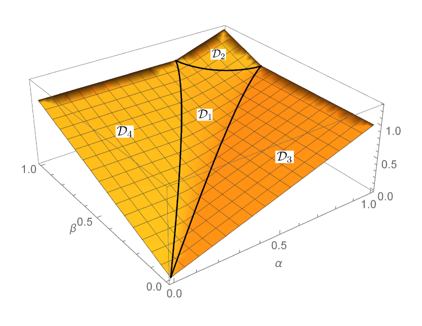
Figure 1: Illustration of $\underline{\Upsilon}^{*}$ for $\rho=0.9$.

$\varphi(s,t)$

$\underline{\Theta}^{*}(s,t)$

$\overline{\Theta}^{*}(s,t)=\psi(s,t)$

Figure 2: Illustration of $\varphi(s,t)$, $\psi(s,t)$, $\underline{\Theta}^{*}(E_{1},E_{2})$, and $\overline{\Theta}^{*}(E_{1},E_{2})$ for the DSBS for $\rho=0.9$. Note that $\underline{\Theta}^{*}(E_{1},E_{2})$ and $\overline{\Theta}^{*}(E_{1},E_{2})$ are expressed in terms of $\varphi(s,t)$ and $\psi(s,t)$ in (44) and (45). All the bases of logarithms are 2 for these figures.

We next provide explicit expressions for $\underline{\Theta}^{*}$ and $\overline{\Theta}^{*}$. Suppose $Q_{X}=(a,1-a)$ and $Q_{Y}=(b,1-b)$. For the DSBS, we have $D(Q_{X}\|P_{X})=1-h(a)$. Hence, if $D(Q_{X}\|P_{X})=s$, then we have $a=h^{-1}(1-s)$ or $1-h^{-1}(1-s)$. Similarly, for $Q_{Y}$ such that $D(Q_{Y}\|P_{Y})=t$, we have $b=h^{-1}(1-t)$ or $1-h^{-1}(1-t)$.

Define $\kappa:=(\frac{1+\rho}{1-\rho})^{2}$. For $\max\{0,a+b-1\}\leq p\leq\min\{a,b\}$, define

$$D_{a,b}(p) :=D((p,a-p,b-p,1+p-a-b)\|$$

$$\qquad(\frac{1+\rho}{4},\frac{1-\rho}{4},\frac{1-\rho}{4},\frac{1+\rho}{4})),$$ (50)

$$\mathsf{D}(a,b) :=\min_{0,a+b-1\leq p\leq a,b}D_{a,b}(p)$$ (51)

$$=D_{a,b}(p^{*}),$$ (52)

where

$$p^{*} =\frac{1}{2(\kappa-1)}\Big{(}(\kappa-1)(a+b)+1$$

$$\quad-\sqrt{((\kappa-1)(a+b)+1)^{2}-4\kappa(\kappa-1)ab}\Big{)}.$$

Equation (52) follows from the facts that $p\mapsto D_{a,b}(p)$ is convex (due to the convexity of the relative entropy), ${\max\{0,a+b-1\}\leq p^{*}\leq\min\{a,b\}}$, and the extreme value is taken at $p^{*}$. Furthermore, we have the following lemma, whose proof is provided in Appendix F.

Lemma 3.

For $0\leq a,b\leq\frac{1}{2}$, it holds that

$$\mathsf{D}(a,b) =\mathsf{D}(1-a,1-b)$$

$$\leq\mathsf{D}(a,1-b)=\mathsf{D}(1-a,b).$$ (53)

By Lemma 3, we have

$$\varphi(s,t) =\mathsf{D}(h^{-1}(1-s),h^{-1}(1-t)),$$

$$\psi(s,t) =\mathsf{D}(h^{-1}(1-s),1-h^{-1}(1-t)),$$

Then $\underline{\Theta}^{*}(E_{1},E_{2})$ and $\overline{\Theta}^{*}(E_{1},E_{2})$ are determined by $\varphi(s,t)$ and $\psi(s,t)$ via (44) and (45). Moreover, by Theorem 4, $\underline{\Theta}(E_{1},E_{2})$ is attained by a sequence involving the time-sharing of at most three pairs of concentric Hamming spheres, and $\overline{\Theta}(E_{1},E_{2})$ is attained by a sequence involving the time-sharing of at most three pairs of anti-concentric Hamming spheres.

Proposition 4 (DSBS).

For the DSBS, the following hold.
1) $\underline{\Theta}(E_{1},E_{2})$ is achieved by a sequence of pairs of concentric Hamming spheres if $\tilde{\varphi}(E_{1},E_{2}):=\min_{s\geq E_{1},t\geq E_{2}}\varphi(s,t)$ is convex in $(E_{1},E_{2})$.
2) $\overline{\Theta}(E_{1},E_{2})$ is achieved by a sequence of pairs of anti-concentric Hamming spheres if $\psi(s,t)$ is concave in $(s,t)$.

Proof:

We prove Proposition 4. For a function $f:\mathbb{R}_{\geq 0}\times\mathbb{R}_{\geq 0}\to\mathbb{R}_{\geq 0}$, we use $\tilde{f}$ to denote $(x,y)\mapsto\inf_{s\geq x,t\geq y}f(s,t)$. Then, by assumption, $\tilde{\varphi}$ is convex. We now prove that $\tilde{\varphi}=\underline{\Theta}^{*}$, where by definition, $\underline{\Theta}^{*}=\tilde{\breve{\varphi}}$. On one hand, $\tilde{\breve{\varphi}}\leq\tilde{\varphi}$. On the other hand, $\tilde{\breve{\varphi}}\geq\tilde{\breve{\tilde{\varphi}}}=\tilde{{\tilde{\varphi}}}={\tilde{\varphi}}$. Hence, $\tilde{\varphi}=\underline{\Theta}^{*}$. This implies that the time-sharing random variable $W$ can be removed. By Theorem 4, time-sharing is not needed to attain $\underline{\Theta}$, completing the proof of Statement 1).

Statement 2) follows similarly, but we need to prove that $\psi(s,t)=\max_{s\leq E_{1},t\leq E_{2}}\psi(s,t)$. This equality is equivalent to that $\max_{Q_{X},Q_{Y}:D(Q_{X}\|P_{X})\leq s,D(Q_{Y}\|P_{Y})\leq t}\mathsf{D}(Q_{X},Q_{Y}\|P_{XY})$ is always attained by some $Q_{X},Q_{Y}$ satisfying that both the equalities in the constraints hold. Observe that in this maximization both the objective function and the constraint functions are convex and, moreover, the set of feasible solutions is compact. By the Krein–Milman theorem, the set of feasible solutions is the closed convex hull of its extreme points. Hence, the maximization is attained by an extreme point. An extreme point here is a pair $(Q_{X},Q_{Y})$ such that $Q_{X}$ is either a Dirac distribution or a distribution satisfying $D(Q_{X}\|P_{X})=s$, and so is $Q_{Y}$. For the DSBS considered here, when $s<1$, there is no Dirac distribution in the set of feasible solutions, which means any extreme points must satisfy $D(Q_{X}\|P_{X})=s$. Similarly, they must also satisfy $D(Q_{Y}\|P_{Y})=t$. These are the desired, which imply Statement 2). ∎

Ordentlich, Polyanskiy, and Shayevitz [17] conjectured that $\underline{\Theta}(E_{1},E_{2})$ is achieved by a sequence of pairs of concentric Hamming spheres, and $\overline{\Theta}(E_{1},E_{2})$ is achieved by a sequence of pairs of anti-concentric Hamming spheres. Hence their conjecture is true under the assumptions in Proposition 4. Given Theorem 4, Ordentlich–Polyanskiy–Shayevitz’s conjecture boils down to proving the convexity of $\tilde{\varphi}$ and concavity of $\psi$. In other words, the essence is to remove the time-sharing random variable $W$ in both $\underline{\Theta}^{*}$ and $\overline{\Theta}^{*}$. Subsequent to the completion of this paper, the first author proved this point, and hence confirmed positively the Ordentlich–Polyanskiy–Shayevitz conjecture [53, 39]. Furthermore, noninteractive simulation in the exponential regime was also studied by Kirshner and Samorodnitsky [18] who solved the symmetric case $E_{1}=E_{2}$.

The functions $\varphi,\psi,\underline{\Theta}^{*}$ and $\overline{\Theta}^{*}$ for $\rho=0.9$ are plotted in Fig. 2. This figure numerically verifies the assumptions in Proposition 4.

III-D Applications to Zero-Error Coding

As mentioned in [17], the minimization part of the conjecture of Ordentlich, Polyanskiy, and Shayevitz implies a sharper outer bound for the zero-error capacity region of the binary adder channel.

Consider the two-user binary adder channel (BAC) $(\mathbf{a},\mathbf{b})\in\{0,1\}^{2n}\mapsto\mathbf{a}+\mathbf{b}\in\{0,1,2\}^{n}$ and a code $(\mathcal{A}_{n},\mathcal{B}_{n})$ with $\mathcal{A}_{n},\mathcal{B}_{n}\subseteq\{0,1\}^{n}$ for this channel. Here $\mathbf{a}+\mathbf{b}$ denotes addition over $\mathbb{Z}^{n}$. When the code $(\mathcal{A}_{n},\mathcal{B}_{n})$ is used to transmit messages over the BAC, the receiver is able to decode the messages without any error if and only if any pair $(\mathbf{a},\mathbf{b})\in\mathcal{A}_{n}\times\mathcal{B}_{n}$ is mapped to a unique sequence in $\{0,1,2\}^{n}$, i.e., $|\mathcal{A}_{n}+\mathcal{B}_{n}|=|\mathcal{A}_{n}|\cdot|\mathcal{B}_{n}|$, where $\mathcal{A}_{n}+\mathcal{B}_{n}$ denotes the sumset $\{\mathbf{a}+\mathbf{b}:\mathbf{a}\in\mathcal{A}_{n},\mathbf{b}\in\mathcal{B}_{n}\}$. The zero-error capacity region $\mathcal{C}$ of the BAC (or the rate region of uniquely decodable code pairs) is defined as the set of $(R_{1},R_{2})$ for which there is a sequence of pairs $\mathcal{A}_{n},\mathcal{B}_{n}\subseteq\{0,1\}^{n}$ with $|\mathcal{A}_{n}|=2^{n(R_{1}+o(1))},|\mathcal{B}_{n}|=2^{n(R_{2}+o(1))}$ such that $|\mathcal{A}_{n}+\mathcal{B}_{n}|=|\mathcal{A}_{n}|\cdot|\mathcal{B}_{n}|$ for every $n$.

Finding the capacity region of the BAC is a long standing open problem; refer to [54, 55, 56, 57, 58, 59, 60, 61, 62, 17] for details. The current progress on this topic is rather unsatisfactory. The upper bound on the sum rate $R_{1}+R_{2}$ is still the simple bound $3/2$, which corresponds to the maximum sum rate in the Shannon capacity. However, Urbanke and Li [59] broke through the $3/2$ bound in the unbalanced case, in which it is assumed that $R_{1}=1$ (note that it does not mean $\mathcal{A}_{n}=\{0,1\}^{n}$) and they showed that $R_{2}\leq 0.4921$. Later, this result was improved to $R_{2}\leq 0.4798$ in [61] and $R_{2}\leq 0.4228$ respectively in [62]. The latter is the best known upper bound until now. The best known lower bound for this case is $R_{2}\geq 1/4$ given in [58].

In particular, the reverse small-set expansion inequality given in (39) for the DSBS was used by Austrin, Kaski, Koivisto, and Nederlof [62] to prove the best known upper bound. As mentioned by Ordentlich, Polyanskiy, and Shayevitz [17], repeating the arguments in [62] with improved bounds on $\overline{\Theta}(E_{1},E_{2})$ will yield tighter bounds on $R_{2}$ when $R_{1}=1$. Replacing the reverse small-set expansion inequality in the proof given in [62] with the characterization of $\overline{\Theta}(E_{1},E_{2})$ in Theorem 4, we obtain the following result.

Theorem 5.

If $(1-\epsilon,R_{2})\in\mathcal{C}$, then for any $\rho\in(0,1)$ there exists some $\lambda\in\frac{1}{2}\pm\sqrt{\frac{\ln(2)\epsilon}{2}}$ such that

$$\lambda\overline{\Theta}^{*}(\frac{\epsilon}{\lambda},\frac{\lambda+\epsilon-R_{2}}{\lambda})$$

$$\geq\lambda(\frac{5}{2}-\log(3-\rho))-\frac{1}{2}-\epsilon-\sqrt{\frac{\ln(2)\epsilon}{2}},$$

where $\overline{\Theta}^{*}$ is defined for the DSBS with correlation coefficient $\rho$. In particular, if $\epsilon=0$, we obtain for any $\rho\in(0,1)$,

$$\frac{1}{2}\overline{\Theta}^{*}(0,1-2R_{2})\geq\frac{1}{2}(\frac{3}{2}-\log(3-\rho)).$$ (54)

Numerical results show that if $R_{1}=1$ (i.e., $\epsilon=0$), by choosing the almost best $\rho=0.6933$, (54) implies $R_{2}\leq 0.4177$, which improves the previously best known bound $R_{2}\leq 0.4228$ established in [62]. Note that the upper bound $R_{2}\leq 0.4177$ was first calculated in [17]. Subsequent to the completion of this paper, $\overline{\Theta}^{*}=\psi$ was proven by the first author [53, 39], which further simplifies the inequalities in Theorem 5.

IV Brascamp–Lieb and Hypercontractivity Inequalities

In this section, we relax Boolean functions in noninteractive simulation problems to any nonnegative functions, but still restrict their supports to be exponentially small. Let $(\mathbf{X},\mathbf{Y})\sim P_{XY}^{n}$, where $P_{XY}$ is a joint distribution defined on $\mathcal{X}\times\mathcal{Y}$. Recall the notation $\langle f,g\rangle=\mathbb{E}[f(\mathbf{X})g(\mathbf{Y})]$ and $\|f\|_{p}=\big{(}\mathbb{E}[f(\mathbf{X})^{p}]\big{)}^{1/p}$. We continue to assume that $\mathcal{X},\mathcal{Y}$ are finite sets, each with cardinality at least $2$, and with $P_{X}(x)>0$, $P_{Y}(y)>0$ for all $(x,y)\in\mathcal{X}\times\mathcal{Y}$. We next derive strengthened versions of (forward and reverse) Brascamp–Lieb and hypercontractivity inequalities by using Theorem 4. Our inequalities reduce to the usual ones when $\alpha=\beta=0$. For $\alpha\in[0,E_{1,\max}],\beta\in[0,E_{2,\max}]$ and $p,q\in(0,\infty)$, define

$$\underline{\Lambda}_{p,q}^{*}(\alpha,\beta) :=\min_{\begin{subarray}{c}\alpha\leq s\leq E_{1,\max}\\ \beta\leq t\leq E_{2,\max}\end{subarray}}(\underline{\Theta}^{*}(s,t)-\frac{s}{p}-\frac{t}{q}),$$

and

$$\overline{\Lambda}_{p,q}^{*}(\alpha,\beta) :=\min_{\begin{subarray}{c}\alpha\leq s\leq E_{1,\max}\\ \beta\leq t\leq E_{2,\max}\end{subarray}}(\frac{s}{p}+\frac{t}{q}-\overline{\Theta}^{*}(s,t)).$$

Remark 10.

Subsequent to the completion of this paper, the first author proved that $\underline{\Theta}^{*}=\tilde{\varphi}$ and $\overline{\Theta}^{*}=\psi$ for the DSBS in [53].

The strengthened (forward and reverse) Brascamp–Lieb inequalities are given in the following theorem, whose proof is provided in Appendix G.

Theorem 6.

Let $p,q>0$ and $\alpha\in[0,E_{1,\max}],\beta\in[0,E_{2,\max}]$. Let $f,g$ be nonnegative functions on $\mathcal{X}^{n}$ and $\mathcal{Y}^{n}$ respectively such that $P_{X}^{n}(\mathrm{supp}(f))\leq 2^{-n\alpha},P_{Y}^{n}(\mathrm{supp}(g))\leq 2^{-n\beta}$. Then

$$\langle f,g\rangle \leq 2^{-n\underline{\Lambda}_{p,q}^{*}(\alpha,\beta)}\|f\|_{p}\|g\|_{q},$$ (55)

$$\langle f,g\rangle \geq 2^{n\overline{\Lambda}_{p,q}^{*}(\alpha,\beta)}\|f\|_{p}\|g\|_{q}.$$ (56)

Remark 11.

Given $\alpha\in[0,E_{1,\max}],\beta\in[0,E_{2,\max}]$ and $p,q>0$, the inequality (55) is exponentially sharp, in the sense that the exponents on the two sides of (55) are asymptotically equal as $n\to\infty$, for a sequence of Boolean functions $f_{n}=1_{\mathcal{A}_{n}},g_{n}=1_{\mathcal{B}_{n}}$ with $(\mathcal{A}_{n},\mathcal{B}_{n})$ denoting the sets given in Remark 7 but with $(E_{1},E_{2})$ there replaced by the optimal $(s^{*},t^{*})$ attaining the minimum in the definition of $\underline{\Lambda}_{p,q}^{*}(\alpha,\beta)$. Note that if $(\alpha,\beta)$ is in the effective region of $\overline{\Theta}^{*}$, then the optimal $(s^{*},t^{*})$ attaining the minimum in the definition of $\overline{\Lambda}_{p,q}^{*}(\alpha,\beta)$ is still in the effective region of $\overline{\Theta}^{*}$. Given $(\alpha,\beta)$ in the effective region of $\overline{\Theta}^{*}$ and $p,q>0$, the inequality (56) is exponentially sharp, in the sense that the exponents on the two sides of (56) are asymptotically equal as $n\to\infty$, for a sequence of Boolean functions $f_{n}=1_{\mathcal{A}_{n}},g_{n}=1_{\mathcal{B}_{n}}$ with some sequence $(\mathcal{A}_{n},\mathcal{B}_{n})$; see Remark 8.

Remark 12.

A special case of Theorem 6 with $p\geq p_{0},q\geq q_{0}$ for (55) and $p\leq p_{1},q\leq q_{1}$ for (55) can be recovered by the information-theoretic characterization of classic Brascamp–Lieb inequalities, where $(\frac{1}{p_{0}},\frac{1}{q_{0}})$ is a subgradient of $\underline{\Theta}^{*}$ and $(\frac{1}{p_{1}},\frac{1}{q_{1}})$ is a subgradient of $\overline{\Theta}^{*}$. See Corollary 3 in [39] which is a consequence of Theorem 2 therein, and also the simple proof of Theorem 2 therein given in Appendix C in [39].

For $\alpha\in[0,E_{1,\max}],\beta\in[0,E_{2,\max}]$, define the forward and reverse $(\alpha,\beta)$-hypercontractivity regions as

$$\mathcal{R}_{\alpha,\beta}^{+}(P_{XY}) :=\{(p,q)\in(0,\infty)^{2}:$$

$$\qquad\underline{\Theta}^{*}(E_{1},E_{2})\geq\frac{1}{p}E_{1}+\frac{1}{q}E_{2},$$

$$\qquad\forall E_{1}\in[\alpha,E_{1,\max}],E_{2}\in[\beta,E_{2,\max}]\},$$

$$\mathcal{R}_{\alpha,\beta}^{-}(P_{XY}) :=\{(p,q)\in(0,\infty)^{2}:$$

$$\qquad\overline{\Theta}^{*}(E_{1},E_{2})\leq\frac{1}{p}E_{1}+\frac{1}{q}E_{2},$$

$$\qquad\forall E_{1}\in[\alpha,E_{1,\max}],E_{2}\in[\beta,E_{2,\max}]\}.$$

For $\alpha=\beta=0$, $\mathcal{R}_{0,0}^{+}(P_{XY})$ and $\mathcal{R}_{0,0}^{-}(P_{XY})$ correspond to the classic hypercontractivity regions in [29, 33, 34, 47] for the forward one and [35, 36, 37, 47, 39] for the reverse one.

As a consequence of Theorem 6, we obtain the following new version of hypercontractivity.

Theorem 7.

Under the assumption in Theorem 6, it holds that

$$\langle f,g\rangle \leq\|f\|_{p}\|g\|_{q},\forall(p,q)\in\mathcal{R}_{\alpha,\beta}^{+}(P_{XY}),$$ (57)

$$\langle f,g\rangle \geq\|f\|_{p}\|g\|_{q},\forall(p,q)\in\mathcal{R}_{\alpha,\beta}^{-}(P_{XY}).$$ (58)

Remark 13.

These two inequalities are exponentially sharp in the same sense as (55) and (56); see Remark 11. That is, given $\alpha\in[0,E_{1,\max}],\beta\in[0,E_{2,\max}]$ and $(p,q)$ in the boundary of $\mathcal{R}_{\alpha,\beta}^{+}(P_{XY})$, the inequality (55) is exponentially sharp, in the sense that the exponents on the two sides of (55) are asymptotically equal as $n\to\infty$, for a sequence of Boolean functions $f_{n}=1_{\mathcal{A}_{n}},g_{n}=1_{\mathcal{B}_{n}}$ with some sequence $(\mathcal{A}_{n},\mathcal{B}_{n})$. Given $(\alpha,\beta)$ in the effective region of $\overline{\Theta}^{*}$ and $(p,q)$ in the boundary of $\mathcal{R}_{\alpha,\beta}^{-}(P_{XY})$, the inequality (56) is exponentially sharp, in the sense that the exponents on the two sides of (56) are asymptotically equal as $n\to\infty$, for a sequence of Boolean functions $f_{n}=1_{\mathcal{A}_{n}},g_{n}=1_{\mathcal{B}_{n}}$ with some sequence $(\mathcal{A}_{n},\mathcal{B}_{n})$.

Note that the hypercontractivity inequalities in Theorem 6 differ from the common ones in the factors $2^{-n\underline{\Lambda}_{p,q}^{*}(\alpha,\beta)}$ and $2^{n\overline{\Lambda}_{p,q}^{*}(\alpha,\beta)}$; while the ones in Theorem 7 differ from the common ones in the region of parameters $p,q$. Strengthening the forward hypercontractivity was previously studied in [42, 18]. Polyanskiy and Samorodnitsky [42] strengthened the hypercontractivity inequalities in a similar sense to Theorem 6; while Kirshner and Samorodnitsky [18] strengthened the hypercontractivity inequalities in a similar sense to Theorem 7. However, both works in [42, 18] focused on strengthening the single-function version of forward hypercontractivity. Moreover, the hypercontractivity inequalities in [42] are only sharp at extreme cases, and only DSBSes were considered in [18]. A systematic investigation of the exponentially sharp version of Brascamp–Lieb and hypercontractivity inequalities in Polish spaces and under a general measure of the “sizes” of functions (termed the two-parameter entropy) was done by the first author in [39].

V Concluding Remarks

The maximal density of subgraphs of a type graph and the biclique rate region have been studied in this paper. One may be also interested in their counterparts—the minimal density of subgraphs of a type graph and the independent-set rate region. Here, given a joint $n$-type $T_{XY}$, $1\leq M_{1}\leq|\mathcal{T}_{T_{X}}|$, and $1\leq M_{2}\leq|\mathcal{T}_{T_{Y}}|$, we define the minimal density of subgraphs of the type graph of $T_{XY}$ with size $(M_{1},M_{2})$ as

$$\underline{\Gamma}_{n}(M_{1},M_{2}) :=\min_{\begin{subarray}{c}\mathcal{A}\subseteq\mathcal{T}_{T_{X}},\mathcal{B}\subseteq\mathcal{T}_{T_{Y}}:\\ |\mathcal{A}|=M_{1},|\mathcal{B}|=M_{2}\end{subarray}}\rho(G[\mathcal{A},\mathcal{B}]).$$

Similar to the biclique rate region, we define the independent-set rate region as

$$\underline{\mathcal{R}}_{n}(T_{XY}) :=\{(R_{1},R_{2})\in\mathcal{R}_{X}^{(n)}\times\mathcal{R}_{Y}^{(n)}:$$

$$\qquad\qquad\underline{\Gamma}_{n}(2^{nR_{1}},2^{nR_{2}})=0\}.$$

Then one can easily obtain the following inner bound and outer bound on $\underline{\mathcal{R}}_{n}(T_{XY})$.

Proposition 5.

For any $n$ and $T_{XY}$,

$$(\underline{\mathcal{R}}^{(i)}(T_{XY})-[0,\varepsilon_{1,n}]\times[0,\varepsilon_{2,n}])\cap(\mathcal{R}_{X}^{(n)}\times\mathcal{R}_{Y}^{(n)})$$

$$\subseteq\underline{\mathcal{R}}_{n}(T_{XY})$$

$$\subseteq\underline{\mathcal{R}}^{(o)}(T_{XY})\cap(\mathcal{R}_{X}^{(n)}\times\mathcal{R}_{Y}^{(n)})$$

for some positive sequences $\{\varepsilon_{1,n}\}$ and $\{\varepsilon_{2,n}\}$ which both vanish as $n\to\infty$, where

$$\underline{\mathcal{R}}^{(o)}(T_{XY}):=\{(R_{1},R_{2}):R_{1}\leq H(X),R_{2}\leq H(Y)\},$$

$$\underline{\mathcal{R}}^{(i)}(T_{XY}):=\bigcup_{\begin{subarray}{c}P_{W},P_{X|W},P_{Y|W}:\\ P_{W}P_{X|W},P_{W}P_{Y|W}\textrm{ are }n\textrm{-types},\\ P_{X}=T_{X},P_{Y}=T_{Y},\\ Q_{XY}\neq T_{XY},\forall Q_{XY|W}\in\mathcal{C}(P_{X|W},P_{Y|W})\end{subarray}}$$

$$\qquad\{(R_{1},R_{2}):R_{1}\leq H(X|W),R_{2}\leq H(Y|W)\}.$$

The inner bound above can be proven by using the codes used in proving the achievability part of Theorem 1. The outer bound above is trivial. Determining the asymptotics of $\underline{\mathcal{R}}_{n}(T_{XY})$ could be of interest. However, currently, we have no idea how to tackle it. In addition, if $\underline{\mathcal{R}}_{n}(T_{XY})$ is not asymptotically equal to $\underline{\mathcal{R}}^{(o)}(T_{XY})$, then determining the exponent of the minimal density is also interesting.

Furthermore, many other fundamental properties of type graphs remain to be investigated, including graph coloring, graph circuits, graph embedding, graph connectivity, covering and packing, etc. [63]. Thanks to good structures enjoyed by type graphs, it seems not hopeless to characterize them.

Appendix A Proof of Lemma 1

Statements 1) and 2) follow directly from the definition of $F^{*}(R_{1},R_{2})$. Note that in Statement 2), the maximum $H_{T}(X,Y)$ is attained by $P_{XYW}=T_{XY}P_{W}$ (or set $W$ to constant) when $R_{1}=H_{T}(X),R_{2}=H_{T}(Y)$.

Statement 3): By symmetry, it suffices to only consider the case $R_{1}=0$. By Statement 2), $F^{*}(0,R_{2})\leq\min\{R_{2},H_{T}(Y|X)\}$. On the other hand, if $R_{2}\geq H_{T}(Y|X)$, then we choose $W=X$, which leads to $H(X|W)=0$ and $H(Y|W)=H(X,Y|W)=H_{T}(Y|X)$. Hence we have $F^{*}(0,R_{2})=H_{T}(Y|X)$ for $R_{2}\geq H_{T}(Y|X)$. If $R_{2}\leq H_{T}(Y|X)$, then one can find a random variable $U$ such that $H(Y|X,U)=R_{2}$. For example, we choose $U=(V,J)$ with $V$ defined on $\mathcal{X}\cup\mathcal{Y}$ and $J$ defined on $\{0,1\}$ such that $V=X$ if $J=0$ and $V=Y$ if $J=1$, where $J\sim\mathrm{Bern}(\alpha)$ for $\alpha:=R_{2}/H_{T}(Y|X)$ is independent of $(X,Y)$. Set $W=(X,U)$. We have $H(X|W)=0$ and $H(Y|W)=H(X,Y|W)=H(X,Y|W,J)=R_{2}$. Hence we have $F^{*}(0,R_{2})=R_{2}$ for $R_{2}\leq H_{T}(Y|X)$.

Statement 4): Let $P_{XYW_{0}}$ attain $F^{*}(R_{1},R_{2})$, and $P_{XYW_{1}}$ attain $F^{*}(\hat{R}_{1},\hat{R}_{2})$. For $0<\alpha<1$, define $J\sim\mathrm{Bern}(\alpha)$ independent of $(X,Y,W_{0},W_{1})$ and let $W:=W_{J}$, taking values in $\mathcal{W}_{0}\cup\mathcal{W}_{1}$, where $\mathcal{W}_{j}$ denotes the alphabet of $W_{j}$ for $j=0,1$. Note that $J$ is a deterministic function of $W$. Then $P_{XYW}$ induces

$$H(X,Y|W) =\alpha H(X,Y|W_{0})+(1-\alpha)H(X,Y|W_{1}),$$

$$H(X|W) =\alpha H(X|W_{0})+(1-\alpha)H(X|W_{1}),$$

$$H(Y|W) =\alpha H(Y|W_{0})+(1-\alpha)H(Y|W_{1}).$$

Therefore,

$$F^{*}(\alpha R_{1}+(1-\alpha)\hat{R}_{1},\alpha R_{2}+(1-\alpha)\hat{R}_{2})$$

$$\geq\alpha F^{*}(R_{1},R_{2})+(1-\alpha)F^{*}(\hat{R}_{1},\hat{R}_{2}).$$

Statement 5): If $\delta_{1}=\delta_{2}=0$, there is nothing to prove. If $\delta_{2}>\delta_{1}=0$, then, for $t\geq 0$,

$$f(t):=F^{*}(R_{1},t)$$

is nondecreasing and concave, by Statements 1) and 4). Hence, for fixed $\delta_{2}$,

$$\frac{f(t+\delta_{2})-f(t)}{\delta_{2}}$$

is nonincreasing in $t$. Combining this with Statements 2) and 3) yields

$$\frac{f(t+\delta_{2})-f(t)}{\delta_{2}}\leq\frac{f(\delta_{2})-f(0)}{\delta_{2}}$$

$$\leq\frac{\delta_{2}+\min\{R_{1},H_{T}(X|Y)\}-\min\{R_{1},H_{T}(X|Y)\}}{\delta_{2}}$$

$$=1.$$

Setting $t=R_{2}$, we obtain $F^{*}(R_{1},R_{2}+\delta_{2})-F^{*}(R_{1},R_{2})\leq\delta_{2}$, as desired.

By symmetry, the claim also holds in the case $\delta_{1}>\delta_{2}=0$. Now we consider the case $\delta_{1},\delta_{2}>0$. Without loss of generality, we assume $\frac{R_{1}}{\delta_{1}}\geq\frac{R_{2}}{\delta_{2}}$. For $t\geq-\frac{R_{2}}{\delta_{2}}$, define

$$g(t):=F^{*}(R_{1}+\delta_{1}t,R_{2}+\delta_{2}t).$$

By Statements 1) and 4), $g(t)$ is nondecreasing and concave. Hence, for fixed $\delta_{2}$,

$$g(t+1)-g(t)$$

is nonincreasing in $t$. Combining this with Statements 2) and 3) yields that for $t\geq-\frac{R_{2}}{\delta_{2}}$ we have

$$g(t+1)-g(t)\leq g(-\frac{R_{2}}{\delta_{2}}+1)-g(-\frac{R_{2}}{\delta_{2}})$$

$$=F^{*}(R_{1}-\frac{\delta_{1}R_{2}}{\delta_{2}}+\delta_{1},\delta_{2})-F^{*}(R_{1}-\frac{\delta_{1}R_{2}}{\delta_{2}},0)$$

$$\leq\min\{R_{1}-\frac{\delta_{1}R_{2}}{\delta_{2}}+\delta_{1},H_{T}(X|Y)\}+\delta_{2}$$

$$\qquad-\min\{R_{1}-\frac{\delta_{1}R_{2}}{\delta_{2}},H_{T}(X|Y)\}$$

$$\leq\delta_{1}+\delta_{2}.$$

Setting $t=0$, we obtain $F^{*}(R_{1}+\delta_{1},R_{2}+\delta_{2})-F^{*}(R_{1},R_{2})\leq\delta_{1}+\delta_{2}$, as desired.

Appendix B Proof of Theorem 1

The claim that we can restrict attention to the case $|\mathcal{W}|\leq|\mathcal{X}||\mathcal{Y}|+2$ in the definition of $F^{*}(R_{1},R_{2})$ comes from the support lemma in [43]. We next prove (12).

Lower bound: Let $\mathcal{C}:=(\mathcal{A}\times\mathcal{B})\cap\mathcal{T}_{T_{XY}}$ for some optimal $(\mathcal{A},\mathcal{B})$ attaining $\Gamma_{n}(2^{nR_{1}},2^{nR_{2}})$. Let $(\mathbf{X},\mathbf{Y})\sim\mathrm{Unif}(\mathcal{C})$. Then,

$$\Gamma_{n}(2^{nR_{1}},2^{nR_{2}}) =\frac{|\mathcal{C}|}{|\mathcal{A}||\mathcal{B}|}=\frac{2^{H(\mathbf{X},\mathbf{Y})}}{2^{nR_{1}}2^{nR_{2}}},$$

$$\frac{1}{n}H(\mathbf{X}) \leq R_{1},$$

$$\frac{1}{n}H(\mathbf{Y}) \leq R_{2},$$

which follow by the fact that the entropy of a random variable is no larger than the logarithm of its support size, and they are equal if the random variable is uniformly distributed over its support. Therefore,

$$E_{n}(R_{1},R_{2}) =R_{1}+R_{2}-\frac{1}{n}H(\mathbf{X},\mathbf{Y})$$

$$=R_{1}+R_{2}-\frac{1}{n}\sum_{i=1}^{n}H(X_{i},Y_{i}|X^{i-1},Y^{i-1})$$

$$=R_{1}+R_{2}-H(X_{J},Y_{J}|X^{J-1},Y^{J-1},J),$$

where $J\sim\mathrm{Unif}[n]$ is a random time index independent of $(X^{n},Y^{n})$ and $X^{J-1}$ denotes a “random vector” induced by $(J,X^{n})$. On the other hand,

$$H(X_{J}|X^{J-1},Y^{J-1},J) \leq H(X_{J}|X^{J-1}J)=\frac{1}{n}H(\mathbf{X})\leq R_{1},$$

$$H(Y_{J}|X^{J-1},Y^{J-1},J) \leq R_{2}.$$

Using the notation

$$X:=X_{J},Y:=Y_{J},W:=(X^{J-1},Y^{J-1},J),$$

we obtain $(X,Y)\sim T_{XY},$ and

$$E_{n}(R_{1},R_{2}) \geq\inf_{\begin{subarray}{c}P_{XYW}:P_{XY}=T_{XY},\\ H(X|W)\leq R_{1},\\ H(Y|W)\leq R_{2}\end{subarray}}R_{1}+R_{2}-H(X,Y|W)$$

$$=E^{*}(R_{1},R_{2}).$$

Upper bound: In this part, we assume that $W$ is a random variable defined on an alphabet $\mathcal{W}$ such that $|\mathcal{W}|\leq|\mathcal{X}||\mathcal{Y}|+2$. For a joint $n$-type $P_{XYW}$ such that $P_{XY}=T_{XY},H(X|W)\leq R_{1},H(Y|W)\leq R_{2}$ and for a fixed sequence $\mathbf{w}$ with type $P_{W}$, we choose $\mathcal{A}$ as the union of $\mathcal{T}_{P_{X|W}}(\mathbf{w})$ and $2^{nR_{1}}-|\mathcal{T}_{P_{X|W}}(\mathbf{w})|$ of arbitrary sequences outside $\mathcal{T}_{P_{X|W}}(\mathbf{w})$, which is possible because $\mathcal{T}_{P_{X|W}}(\mathbf{w})\leq 2^{nH(X|W)}$, see [3, Lemma 2.5], and choose $\mathcal{B}$ in a similar way, but with $\mathcal{T}_{P_{X|W}}(\mathbf{w})$ replaced by $\mathcal{T}_{P_{Y|W}}(\mathbf{w})$. Then $|\mathcal{A}|=2^{nR_{1}}$ and $|\mathcal{B}|=2^{nR_{2}}$. Observe that

$$|(\mathcal{A}\times\mathcal{B})\cap\mathcal{T}_{T_{XY}}| \geq|\mathcal{T}_{P_{XY|W}}(\mathbf{w})|$$

$$\geq 2^{n(H(X,Y|W)-\frac{|\mathcal{W}||\mathcal{X}||\mathcal{Y}|\log(n+1)}{n})},$$

where

• the first inequality follows since for any pair $(\mathbf{x},\mathbf{y})\in\mathcal{T}_{P_{XY|W}}(\mathbf{w})$, the tuple $(\mathbf{w},\mathbf{x},\mathbf{y})$ must have joint type $P_{WXY}$, and hence, $(\mathbf{w},\mathbf{x})$ has joint type $P_{WX}$, $(\mathbf{w},\mathbf{y})$ has joint type $P_{WY}$, and $(\mathbf{x},\mathbf{y})$ has joint type $T_{XY}$;

• the second inequality follows from [3, Lemma 2.5].

Thus we have

$$\rho(G[\mathcal{A},\mathcal{B}]) =\frac{|(\mathcal{A}\times\mathcal{B})\cap\mathcal{T}_{T_{XY}}|}{2^{nR_{1}}2^{nR_{2}}}$$

$$\geq 2^{-n(R_{1}+R_{2}-H(X,Y|W)+\frac{|\mathcal{W}||\mathcal{X}||\mathcal{Y}|\log(n+1)}{n})}.$$ (59)

Optimizing the exponent in (59) over all joint $n$-types $P_{XYW}$ such that $P_{XY}=T_{XY},H(X|W)\leq R_{1},H(Y|W)\leq R_{2}$ yields the upper bound

$$E_{n}(R_{1},R_{2}) \leq R_{1}+R_{2}-F_{n}(R_{1},R_{2})$$

$$\qquad+\frac{|\mathcal{W}||\mathcal{X}||\mathcal{Y}|\log(n+1)}{n},$$ (60)

where $F_{n}(R_{1},R_{2})$ is defined similarly as $F^{*}(R_{1},R_{2})$ in (10) but with the $P_{XYW}$ in (10) restricted to be a joint $n$-type and $\mathcal{W}$ assumed to satisfy $|\mathcal{W}|\leq|\mathcal{X}||\mathcal{Y}|+2$.

We next show that the values of $F_{n}(R_{1},R_{2})$ and $F^{*}(R_{1},R_{2})$ do not differ too much. For a joint $n$-type $T_{XY}$ and a distribution $P_{XYW}$ with $P_{XY}=T_{XY}$, one can find a $n$-type $Q_{XYW}$ with $Q_{XY}=T_{XY}$ such that $\|P_{XYW}-Q_{XYW}\|\leq\frac{|\mathcal{W}||\mathcal{X}||\mathcal{Y}|}{2n}$, where $\|\cdot\|$ denotes the TV distance, see [64, Lemma 3]. Combining this with [3, Lemma 2.7] (i.e., if $\|P_{X}-Q_{X}\|\leq\Theta\leq\frac{1}{4}$, then $|H_{P}(X)-H_{Q}(X)|\leq-2\Theta\log\frac{2\Theta}{|\mathcal{X}|}$), we have for $\frac{|\mathcal{W}||\mathcal{X}||\mathcal{Y}|}{2n}\leq\frac{1}{4}$ that

$$|H_{P}(X|W)-H_{Q}(X|W)|$$

$$\leq|H_{P}(X,W)-H_{Q}(X,W)|+|H_{P}(W)-H_{Q}(W)|$$

$$\leq-2\frac{|\mathcal{W}||\mathcal{X}||\mathcal{Y}|}{2n}\log\frac{2\frac{|\mathcal{W}||\mathcal{X}||\mathcal{Y}|}{2n}}{|\mathcal{X}||\mathcal{W}|}$$

$$\qquad-2\frac{|\mathcal{W}||\mathcal{X}||\mathcal{Y}|}{2n}\log\frac{2\frac{|\mathcal{W}||\mathcal{X}||\mathcal{Y}|}{2n}}{|\mathcal{W}|}$$ (61)

$$=-\frac{|\mathcal{W}||\mathcal{X}||\mathcal{Y}|}{n}\log\frac{|\mathcal{X}||\mathcal{Y}|^{2}}{n^{2}},$$ (62)

and similarly,

$$|H_{P}(Y|W)-H_{Q}(Y|W)| \leq-\frac{|\mathcal{W}||\mathcal{X}||\mathcal{Y}|}{n}\log\frac{|\mathcal{X}|^{2}|\mathcal{Y}|}{n^{2}},$$ (63)

$$|H_{P}(XY|W)-H_{Q}(XY|W)| \leq-\frac{|\mathcal{W}||\mathcal{X}||\mathcal{Y}|}{n}\log\frac{|\mathcal{X}||\mathcal{Y}|}{n^{2}}.$$ (64)

Combining (62)-(64) yields that

$$F_{n}(R_{1},R_{2}) \geq F^{*}(R_{1}+\frac{|\mathcal{W}||\mathcal{X}||\mathcal{Y}|}{n}\log\frac{|\mathcal{X}||\mathcal{Y}|^{2}}{n^{2}},$$

$$\qquad R_{2}+\frac{|\mathcal{W}||\mathcal{X}||\mathcal{Y}|}{n}\log\frac{|\mathcal{X}|^{2}|\mathcal{Y}|}{n^{2}})$$

$$\qquad+\frac{|\mathcal{W}||\mathcal{X}||\mathcal{Y}|}{n}\log\frac{|\mathcal{X}||\mathcal{Y}|}{n^{2}}.$$

Applying Statement 5) of Lemma 1, we obtain

$$F_{n}(R_{1},R_{2}) \geq F^{*}(R_{1},R_{2})+\frac{|\mathcal{W}||\mathcal{X}||\mathcal{Y}|}{n}\log\frac{|\mathcal{X}|^{4}|\mathcal{Y}|^{4}}{n^{6}}.$$

Substituting this into the upper bound in (60) and combining with the assumption $|\mathcal{W}|\leq|\mathcal{X}||\mathcal{Y}|+2$ yields the desired upper bound.

Appendix C Proof of Theorem 2

We now prove Theorem 2. Since (19) follows from (18), it suffices to prove (18).

Inner Bound: The inner bound proof here uses a standard time-sharing argument. Let $d$ be an integer such that $1\leq d\leq n-1$. Let $(P_{XY},Q_{XY})$ be a pair comprised of a $d$-joint type and an $(n-d)$-joint type on $\mathcal{X}\times\mathcal{Y}$ such that $\frac{d}{n}P_{XY}+(1-\frac{d}{n})Q_{XY}=T_{XY}$. For a fixed length-$d$ sequence $\mathbf{y}$ with type $P_{Y}$ an a fixed length-$(n-d)$ sequence $\mathbf{x}$ with type $Q_{X}$, we choose $\mathcal{A}=\mathcal{T}_{P_{X|Y}}(\mathbf{y})\times\{\mathbf{x}\}$ and $\mathcal{B}=\{\mathbf{y}\}\times\mathcal{T}_{Q_{Y|X}}(\mathbf{x})$. Then, from [3, Lemma 2.5], we have $|\mathcal{A}|\geq 2^{d(H_{P}(X|Y)-\frac{|\mathcal{X}||\mathcal{Y}|\log(d+1)}{d})}$ and similarly $|\mathcal{B}|\geq 2^{(n-d)(H_{Q}(Y|X)-\frac{|\mathcal{X}||\mathcal{Y}|\log(n-d+1)}{n-d})}$. On the other hand, for this code we have $\mathcal{A}\times\mathcal{B}\subseteq\mathcal{T}_{T_{XY}}$. Hence any rate pair $(R_{1},R_{2})\in(\mathcal{R}_{X}^{(n)}\times\mathcal{R}_{Y}^{(n)})$ with

$$R_{1} \leq\frac{d}{n}(H_{P}(X|Y)-\frac{|\mathcal{X}||\mathcal{Y}|\log(d+1)}{d}),$$

$$R_{2} \leq(1-\frac{d}{n})(H_{Q}(Y|X)-\frac{|\mathcal{X}||\mathcal{Y}|\log(n-d+1)}{n-d}),$$

is achievable (i.e., it is in $\mathcal{R}_{n}(T_{XY})$), which in turn implies that a pair of smaller rates $(R_{1},R_{2})\in(\mathcal{R}_{X}^{(n)}\times\mathcal{R}_{Y}^{(n)})$ with

$$R_{1} \leq\frac{d}{n}H_{P}(X|Y)-\frac{|\mathcal{X}||\mathcal{Y}|\log(n+1)}{n},$$ (65)

$$R_{2} \leq(1-\frac{d}{n})H_{Q}(Y|X)-\frac{|\mathcal{X}||\mathcal{Y}|\log(n+1)}{n},$$ (66)

is achievable.

We next remove the constraint that $(P_{XY},Q_{XY})$ are joint types. For $0\leq\alpha\leq 1$, let $(\hat{P}_{XY},\hat{Q}_{XY})$ be a pair of distributions such that $\alpha\hat{P}_{XY}+(1-\alpha)\hat{Q}_{XY}=T_{XY}$. Define $d:=\|\lfloor n\alpha\hat{P}_{XY}\rfloor\|_{1}$. Note that we have

$$n\alpha-|\mathcal{X}||\mathcal{Y}|\leq d\leq n\alpha.$$ (67)

We first consider the case

$$4|\mathcal{X}||\mathcal{Y}|\leq d\leq n-4|\mathcal{X}||\mathcal{Y}|.$$ (68)

Define $P_{XY}:=\frac{\lfloor n\alpha\hat{P}_{XY}\rfloor}{d}$. Then $P_{XY}$ is a joint $d$-type and $\|P_{XY}-\hat{P}_{XY}\|\leq\frac{|\mathcal{X}||\mathcal{Y}|}{d}\leq\frac{1}{4}$. Define $Q_{XY}:=\frac{nT_{XY}-dP_{XY}}{n-d}$, which is a joint $(n-d)$-type and satisfies $\|Q_{XY}-\hat{Q}_{XY}\|\leq\frac{|\mathcal{X}||\mathcal{Y}|}{n-d}\leq\frac{1}{4}$. Combining [3, Lemma 2.7] with the equality $H(X|Y)=H(X,Y)-H(Y)$, we have

$$H_{P}(X|Y) \geq H_{\hat{P}}(X|Y)+\frac{2|\mathcal{X}||\mathcal{Y}|}{d}\log\frac{4|\mathcal{X}|}{d^{2}},$$

$$H_{Q}(Y|X) \geq H_{\hat{Q}}(Y|X)+\frac{2|\mathcal{X}||\mathcal{Y}|}{n-d}\log\frac{4|\mathcal{Y}|}{(n-d)^{2}}.$$

These inequalities, together with (65) and (66), imply that

$$\textrm{RHS of }\eqref{eq:-53} \geq\frac{d}{n}H_{\hat{P}}(X|Y)-\frac{2|\mathcal{X}||\mathcal{Y}|}{n}\log\frac{n^{2}}{4|\mathcal{X}|}$$

$$\qquad-\frac{|\mathcal{X}||\mathcal{Y}|\log(n+1)}{n}$$ (69)

$$\geq\alpha H_{\hat{P}}(X|Y)-\frac{|\mathcal{X}||\mathcal{Y}|}{n}\log|\mathcal{X}|$$

$$\qquad-\frac{2|\mathcal{X}||\mathcal{Y}|}{n}\log\frac{n^{2}}{4|\mathcal{X}|}$$

$$\qquad-\frac{|\mathcal{X}||\mathcal{Y}|\log(n+1)}{n}$$ (70)

$$=\alpha H_{\hat{P}}(X|Y)-\epsilon_{1,n};$$ (71)

$$\textrm{RHS of }\eqref{eq:-52} \geq(1-\frac{d}{n})H_{\hat{Q}}(Y|X)-\frac{2|\mathcal{X}||\mathcal{Y}|}{n}\log\frac{n^{2}}{4|\mathcal{Y}|}$$

$$\qquad-\frac{|\mathcal{X}||\mathcal{Y}|\log(n+1)}{n}$$ (72)

$$\geq(1-\alpha)H_{\hat{Q}}(Y|X)-\frac{2|\mathcal{X}||\mathcal{Y}|}{n}\log\frac{n^{2}}{4|\mathcal{Y}|}$$

$$\qquad-\frac{|\mathcal{X}||\mathcal{Y}|\log(n+1)}{n}$$ (73)

$$=(1-\alpha)H_{\hat{Q}}(Y|X)-\epsilon_{2,n}.$$ (74)

Recall the definitions of $\epsilon_{1,n}$ and $\epsilon_{2,n}$ in Theorem 2.

Combining (65), (66), (71), and (74) yields that any rate pair $(R_{1},R_{2})\in(\mathcal{R}_{X}^{(n)}\times\mathcal{R}_{Y}^{(n)})$ with $R_{1}\leq\alpha H_{\hat{P}}(X|Y)-\epsilon_{1,n}$ and $R_{2}\leq(1-\alpha)H_{\hat{Q}}(Y|X)-\epsilon_{2,n}$, for any $0\leq\alpha\leq 1$ and $(\hat{P}_{XY},\hat{Q}_{XY})$ a pair of distributions such that $\alpha\hat{P}_{XY}+(1-\alpha)\hat{Q}_{XY}=T_{XY}$, is achievable as long as the condition in (68) holds.

We next consider the case $0\leq d<4|\mathcal{X}||\mathcal{Y}|$. For this case, we have

$$\alpha H_{\hat{P}}(X|Y) \leq\frac{d+|\mathcal{X}||\mathcal{Y}|}{n}\log|\mathcal{X}|$$

$$\leq\frac{5|\mathcal{X}||\mathcal{Y}|}{n}\log|\mathcal{X}|\leq\varepsilon_{1,n},$$

where the first inequality follows by (67) and the fact that $H_{\hat{P}}(X|Y)\leq\log|\mathcal{X}|$. Hence

$$\{(R_{1},R_{2}):R_{1}\leq\alpha H_{\hat{P}}(X|Y),R_{2}\leq(1-\alpha)H_{\hat{Q}}(Y|X)\}$$

$$\qquad-[0,\varepsilon_{1,n}]\times[0,\varepsilon_{2,n}]$$

is empty, and so its intersection with $(\mathcal{R}_{X}^{(n)}\times\mathcal{R}_{Y}^{(n)})$ is also empty. Therefore, there is nothing to prove in this case. The case when $n-4|\mathcal{X}||\mathcal{Y}|<d\leq n$ can be handled similarly. This completes the proof for the inner bound.

Outer Bound: We next prove the outer bound by combining information-theoretic methods and linear algebra. Observe that the biclique rate region only depends on the probability values of $T_{XY}$, rather than the alphabets $\mathcal{X},\mathcal{Y}$. With this in mind, we observe that we can identify $\mathcal{X}$ and $\mathcal{Y}$ with subsets of $\mathbb{R}$ by one-to-one mappings such that, for any probability distribution $P_{XY}$, if $(X,Y)\in\mathcal{X}\times\mathcal{Y}$ satisfies $(X,Y)\sim P_{XY}$ we can talk about the expectations $\mathbb{E}_{P}[X]$, $\mathbb{E}_{P}[Y]$, the covariance $\mbox{Cov}_{P}(X,Y)$, and the correlation $\mathbb{E}_{P}[XY]$. Translating the choices of $\mathcal{X}$ and/or $\mathcal{Y}$ (as subsets of $\mathbb{R}$) does not change $\mbox{Cov}_{P}(X,Y)$, so we can ensure that we make these choices in such a way that $\mathbb{E}_{P}[XY]=\mbox{Cov}_{P}(X,Y)+\mathbb{E}_{P}[X]\mathbb{E}_{P}[Y]=0$.

Let us now choose $\mathcal{X},\mathcal{Y}\subseteq\mathbb{R}$ in this way, such that for the given joint $n$-type $T_{XY}$ we have $E_{T}[XY]=0$. Then, for $\mathcal{A}\times\mathcal{B}\subseteq\mathcal{T}_{T_{XY}}$, we will have $\langle\mathbf{x},\mathbf{y}\rangle=0$ for any $(\mathbf{x},\mathbf{y})\in\mathcal{A}\times\mathcal{B}$, where $\mathbf{x},\mathbf{y}$ are now viewed as row vectors in $\mathbb{R}^{n}$. Let $\overline{\mathcal{A}}$ denote the linear space spanned by all the vectors in $\mathcal{A}$, and let $\overline{\mathcal{B}}$ denote the linear space spanned by all the vectors in $\mathcal{B}$. Hence $\overline{\mathcal{B}}\subseteq\overline{\mathcal{A}}^{\perp}$, where $\overline{\mathcal{A}}^{\perp}$ denotes the orthogonal complement of a subspace $\overline{\mathcal{A}}$. As an important property of the orthogonal complement, $\dim(\overline{\mathcal{A}})+\dim(\overline{\mathcal{A}}^{\bot})=n.$ Hence $\dim(\overline{\mathcal{A}})+\dim(\overline{\mathcal{B}})\leq n.$

We next establish the following exchange lemma. The proof is provided in Appendix D, and is based on the well-known exchange lemma in linear algebra.

Lemma 4.

Let $\mathcal{V}_{1},\mathcal{V}_{2}$ be mutually orthogonal linear subspaces of $\mathbb{R}^{n}$ with dimensions, denoted as $n_{1},n_{2}$, satisfying $n_{1}+n_{2}=n$. Then there always exists a partition $\{\mathcal{J}_{1},\mathcal{J}_{2}\}$ of $[n]$ such that $|\mathcal{J}_{i}|=n_{i}$ and $\mathbf{x}=f_{i}(\mathbf{x}_{\mathcal{J}_{i}}),\forall\mathbf{x}\in\mathcal{V}_{i},i=1,2$ for some deterministic linear functions $f_{i}:\mathbb{R}^{n_{i}}\to\mathbb{R}^{n}$, where $\mathbf{x}_{\mathcal{J}_{i}}:=(x_{j})_{j\in\mathcal{J}_{i}}$.

Remark 14.

The natural generalization of this lemma also holds for $k$ mutually orthogonal linear subspaces of $\mathbb{R}^{n}$ with total dimensions equal to $n$, and can be proved using Lemma 5 in Appendix D. Furthermore, the condition “mutually orthogonal linear subspaces of $\mathbb{R}^{n}$” can be replaced by “mutually (linearly) independent linear subspaces of $\mathbb{R}^{n}$” (i.e., such that the dimension of the span of the subspaces equals the sum of the dimensions of the subspaces), or, more generally, affine subspaces each of which is a translate of one of a mutually independent family of linear subspaces of $\mathbb{R}^{n}$.

Remark 15.

In other words, under the assumption in this lemma there always exists a permutation $\sigma$ of $[n]$ such that $\mathbf{x}^{(\sigma)}=f_{1}(\mathbf{x}_{[1:n_{1}]}^{(\sigma)}),\forall\mathbf{x}\in V_{1}$ and $\mathbf{x}^{(\sigma)}=f_{2}(\mathbf{x}_{[n_{1}+1:n]}^{(\sigma)}),\forall\mathbf{x}\in V_{2}$ for some deterministic functions $f_{i}:\mathbb{R}^{n_{i}}\to\mathbb{R}^{n}$, where $\mathbf{x}^{(\sigma)}$ is obtained by permuting the components of $\mathbf{x}$ using $\sigma$.

Let $d$ denote $\dim(\overline{\mathcal{A}})$, so we have $\dim(\overline{\mathcal{A}}^{\bot})=n-d$. Let $\mathbf{X}\sim\mathrm{Unif}(\mathcal{A}),\mathbf{Y}\sim\mathrm{Unif}(\mathcal{B})$ be two independent random vectors, i.e., $(\mathbf{X},\mathbf{Y})\sim P_{\mathbf{X},\mathbf{Y}}:=\mathrm{Unif}(\mathcal{A})\mathrm{Unif}(\mathcal{B})$. Now we choose $V_{1}=\overline{\mathcal{A}},V_{2}=\overline{\mathcal{A}}^{\bot},\mathbf{X}_{1}=\mathbf{X},\mathbf{X}_{2}=\mathbf{Y}$ in Lemma 4. Then there exists a partition $\{\mathcal{J},\mathcal{J}^{c}\}$ of $[n]$ such that $|\mathcal{J}|=d$ and $\mathbf{X}=f_{1}(\mathbf{X}_{\mathcal{J}}),\mathbf{Y}=f_{2}(\mathbf{Y}_{\mathcal{J}^{c}})$ for some deterministic functions $f_{1}:\mathbb{R}^{d}\to\mathbb{R}^{n},f_{2}:\mathbb{R}^{n-d}\to\mathbb{R}^{n}$. By this property, on the one hand we have

$$R_{1} =\frac{1}{n}H(\mathbf{X})=\frac{1}{n}H(\mathbf{X}|\mathbf{Y})=\frac{1}{n}H(\mathbf{X}_{\mathcal{J}}|\mathbf{Y})$$

$$\leq\frac{1}{n}H(\mathbf{X}_{\mathcal{J}}|\mathbf{Y}_{\mathcal{J}})\leq\frac{1}{n}\sum_{j\in\mathcal{J}}H(X_{j}|Y_{j})$$

$$=\frac{d}{n}H(X_{J}|Y_{J},J)\leq\frac{d}{n}H(X_{J}|Y_{J})=\frac{d}{n}H(\tilde{X}|\tilde{Y}),$$

where $J\sim\mathrm{Unif}(\mathcal{J})$, $\tilde{X}:=X_{J},\tilde{Y}:=Y_{J}$, with $J$ being independent of $(\mathbf{X},\mathbf{Y})$. Similarly, we have

$$R_{2} =\frac{1}{n}H(\mathbf{Y})=\frac{1}{n}H(\mathbf{Y}|\mathbf{X})=\frac{1}{n}H(\mathbf{Y}_{\mathcal{J}^{c}}|\mathbf{X})$$

$$\leq\frac{1}{n}H(\mathbf{Y}_{\mathcal{J}^{c}}|\mathbf{X}_{\mathcal{J}^{c}})\leq\frac{1}{n}\sum_{j\in\mathcal{J}^{c}}H(Y_{j}|X_{j})$$

$$=(1-\frac{d}{n})H(Y_{\hat{J}}|X_{\hat{J}},\hat{J})$$

$$\leq(1-\frac{d}{n})H(Y_{\hat{J}}|X_{\hat{J}})=(1-\frac{d}{n})H(\hat{Y}|\hat{X}),$$

where $\hat{J}\sim\mathrm{Unif}(\mathcal{J}^{c})$, $\hat{X}:=X_{\hat{J}},\hat{Y}:=Y_{\hat{J}}$, with $\hat{J}$ being independent of $(\mathbf{X},\mathbf{Y},J)$. On the other hand,

$$\frac{d}{n}P_{\tilde{X}\tilde{Y}}+(1-\frac{d}{n})P_{\hat{X}\hat{Y}}$$

$$=\frac{1}{n}\sum_{j\in\mathcal{J}}P_{X_{j}Y_{j}}+\frac{1}{n}\sum_{j\in\mathcal{J}^{c}}P_{X_{j}Y_{j}}$$

$$=\frac{1}{n}\sum_{j=1}^{n}P_{X_{j}Y_{j}}=\mathbb{E}_{(\mathbf{X},\mathbf{Y})}[T_{\mathbf{XY}}]=T_{XY},$$

where $T_{\mathbf{XY}}$ denotes the joint type of a random pair $(\mathbf{X},\mathbf{Y})$ which is hence also random (but equals $T_{XY}$ pointwise). This completes the proof of the outer bound.

Appendix D Proof of Lemma 4

For a pair of orthogonal subspaces $(\mathcal{V},\mathcal{V}^{\perp})$ with dimensions respectively $n_{1},n-n_{1}$, let $\{\mathbf{u}_{j}:1\leq j\leq n_{1}\}$ be an orthogonal basis of $\mathcal{V}$, and $\{\mathbf{u}_{j}:n_{1}+1\leq j\leq n\}$ be an orthogonal basis of $\mathcal{V}^{\perp}$. Then $\{\mathbf{u}_{j}:1\leq j\leq n\}$ forms an orthogonal basis of $\mathbb{R}^{n}$. Denote by $\boldsymbol{\mathbf{U}}$ the $n\times n$ matrix with $j$-th row being $\mathbf{u}_{j}$. Then $\boldsymbol{\mathbf{U}}$ is orthogonal. We now express $\mathbf{x}\in\mathcal{V}$ and $\mathbf{y}\in\mathcal{V}^{\perp}$, thought of as row vectors, in terms of this orthogonal basis, i.e.,

$$\mathbf{x}=\hat{\mathbf{x}}\boldsymbol{\mathbf{U}},\qquad\mathbf{y}=\hat{\mathbf{y}}\boldsymbol{\mathbf{U}},$$ (75)

where $\hat{\mathbf{x}}:=\mathbf{x}\boldsymbol{\mathbf{U}}^{\top},\hat{\mathbf{y}}:=\mathbf{y}\boldsymbol{\mathbf{U}}^{\top}$, and $\boldsymbol{\mathbf{U}}^{\top}$ is the transpose of $\boldsymbol{\mathbf{U}}$. Since for any $\mathbf{x}\in\mathcal{V}$ we have $\langle\mathbf{x},\mathbf{u}_{j}\rangle=0$ for all $n_{1}+1\leq j\leq n$, we obtain that $\hat{x}_{j}=0$ for all $n_{1}+1\leq j\leq n$. Similarly, $\hat{y}_{j}=0$ for all $1\leq j\leq n_{1}$. Hence we can rewrite $\hat{\mathbf{x}}=(\hat{\mathbf{x}}_{1},\mathbf{0}),\hat{\mathbf{y}}=(\mathbf{0},\hat{\mathbf{y}}_{2})$. We write $\boldsymbol{\mathbf{U}}$ in a block form: $\boldsymbol{\mathbf{U}}=\begin{bmatrix}\boldsymbol{\mathbf{U}}_{1}\\ \boldsymbol{\mathbf{U}}_{2}\end{bmatrix}$ where $\boldsymbol{\mathbf{U}}_{1},\boldsymbol{\mathbf{U}}_{2}$ are respectively of size $n_{1}\times n,(n-n_{1})\times n$. Then

$$\mathbf{x}=\hat{\mathbf{x}}_{1}\boldsymbol{\mathbf{U}}_{1},\qquad\mathbf{y}=\hat{\mathbf{y}}_{2}\boldsymbol{\mathbf{U}}_{2}.$$ (76)

We now need the following well-known exchange lemma.

Lemma 5 (Exchange Lemma).

[65, Theorem 3.2] Let $k\geq 2$ be an integer. Let $\mathbf{B}$ be an $n\times n$ nonsingular matrix, and $\{\mathcal{H}_{l},1\leq l\leq k\}$ be a partition of $[n]$. Then there always exists another partition $\{\mathcal{L}_{l},1\leq l\leq k\}$ of $[n]$ with $|\mathcal{L}_{l}|=|\mathcal{H}_{l}|$ such that all the sub-matrices $\mathbf{B}_{\mathcal{H}_{l},\mathcal{L}_{l}},1\leq l\leq k$ are nonsingular.

The proof of this lemma follows easily from repeated use of the Laplace expansion for determinants. A short proof in the case $k=2$, which is the only case we use, goes as follows. Let $\mathbf{B}=(b_{i,j})$ be an $n\times n$ matrix and $\mathcal{H}$ a subset of $[n]$. Then the determinant of $\mathbf{B}$ can be expanded as follows:

$$\det(\mathbf{B})=\sum_{\mathcal{L}\subseteq[n]:|\mathcal{L}|=|\mathcal{H}|}\varepsilon^{\mathcal{H},\mathcal{L}}\det(\mathbf{B}_{\mathcal{H},\mathcal{L}})\det(\mathbf{B}_{\mathcal{H}^{c},\mathcal{L}^{c}})$$

where $\varepsilon^{\mathcal{H},\mathcal{L}}$ is the sign of the permutation determined by $\mathcal{H}$ and $\mathcal{L}$, equal to $(-1)^{(\sum_{h\in\mathcal{H}}h)+(\sum_{\ell\in\mathcal{L}}\ell)}$. Since $\mathbf{B}$ is nonsingular, there must be at least one choice of $|\mathcal{L}|$, with $|\mathcal{L}|=|\mathcal{H}|$, such that both $\mathbf{B}_{\mathcal{H},\mathcal{L}}$ and $\mathbf{B}_{\mathcal{H}^{c},\mathcal{L}^{c}}$ are nonsingular, which is what is being claimed.

Substituting $\mathbf{B}\leftarrow\boldsymbol{\mathbf{U}},\mathcal{H}_{1}\leftarrow[n_{1}],\mathcal{H}_{2}\leftarrow[n_{1}+1:n]$ in this lemma, we obtain that there exists a partition $\{\mathcal{J},\mathcal{J}^{c}\}$ of $[n]$ with $|\mathcal{J}|=n_{1}$ such that both the sub-matrices $\mathbf{U}_{[n_{1}],\mathcal{J}},\mathbf{U}_{[n_{1}+1:n],\mathcal{J}^{c}}$ are nonsingular. Denote $\boldsymbol{\mathbf{U}}_{1,\mathcal{J}}$ as the submatrix of $\boldsymbol{\mathbf{U}}_{1}$ consisting of $\mathcal{J}$- indexed columns of $\boldsymbol{\mathbf{U}}_{1}$, and define $\boldsymbol{\mathbf{U}}_{1,\mathcal{J}^{c}},\boldsymbol{\mathbf{U}}_{2,\mathcal{J}},\boldsymbol{\mathbf{U}}_{2,\mathcal{J}^{c}}$ similarly. Then, by definition, $\boldsymbol{\mathbf{U}}_{1,\mathcal{J}}=\mathbf{U}_{[n_{1}],\mathcal{J}},\boldsymbol{\mathbf{U}}_{2,\mathcal{J}^{c}}=\mathbf{U}_{[n_{1}+1:n],\mathcal{J}^{c}}$. Therefore, from (76), we have

$$\hat{\mathbf{x}}_{1}=\mathbf{x}_{\mathcal{J}}\boldsymbol{\mathbf{U}}_{1,\mathcal{J}}^{-1},\qquad\hat{\mathbf{y}}_{2}=\mathbf{y}_{\mathcal{J}^{c}}\boldsymbol{\mathbf{U}}_{2,\mathcal{J}^{c}}^{-1}.$$

Substituting these back into (76), we obtain that

$$(\mathbf{x}_{\mathcal{J}},\mathbf{x}_{\mathcal{J}^{c}}) =\mathbf{x}_{\mathcal{J}}\boldsymbol{\mathbf{U}}_{1,\mathcal{J}}^{-1}(\boldsymbol{\mathbf{U}}_{1,\mathcal{J}},\boldsymbol{\mathbf{U}}_{1,\mathcal{J}^{c}})$$

$$=(\mathbf{x}_{\mathcal{J}},\mathbf{x}_{\mathcal{J}}\boldsymbol{\mathbf{U}}_{1,\mathcal{J}}^{-1}\boldsymbol{\mathbf{U}}_{1,\mathcal{J}^{c}})$$

and

$$(\mathbf{y}_{\mathcal{J}},\mathbf{y}_{\mathcal{J}^{c}})=(\mathbf{y}_{\mathcal{J}^{c}}\boldsymbol{\mathbf{U}}_{2,\mathcal{J}^{c}}^{-1}\boldsymbol{\mathbf{U}}_{2,\mathcal{J}},\mathbf{y}_{\mathcal{J}^{c}}).$$

Hence the proof is completed.

Appendix E Proof of Proposition 2

From Theorem 2, we know that $\mathcal{R}(T_{XY})=\mathcal{R}^{*}(T_{XY})$, where $\mathcal{R}(T_{XY})$ is the asymptotic biclique rate region, defined in (7) and $\mathcal{R}^{*}(T_{XY})$ is defined in Theorem 2. Furthermore, $\mathcal{R}^{*}(T_{XY})$ is a closed convex set (see Proposition 1). Hence

$$\mathcal{R}(T_{XY})=\mathcal{R}_{\bigtriangleup}(T_{XY})$$

if and only if

$$\max_{\begin{subarray}{c}0\leq\alpha\leq 1,P_{XY},Q_{XY}:\\ \alpha P_{XY}+(1-\alpha)Q_{XY}=T_{XY}\end{subarray}}\varphi_{\alpha}(P_{XY},Q_{XY})\leq 1,$$ (77)

where $\varphi_{\alpha}(P_{XY},Q_{XY}):=\frac{\alpha}{\beta_{1}}H_{P}(X|Y)+\frac{1-\alpha}{\beta_{2}}H_{Q}(Y|X)$ with $\beta_{1}:=H_{T}(X|Y),\beta_{2}:=H_{T}(Y|X)$. Here the domain of $\varphi_{\alpha}$ can be taken to be the set of pairs of probability distributions $(P_{XY},Q_{XY})$ such that $\mathrm{supp}(P_{XY})=\mathrm{supp}(Q_{XY})\subseteq\mathrm{supp}(T_{XY})$. Moreover, (77) can be rewritten as that for any $0\leq\alpha\leq 1,$

$$\max_{P_{XY},Q_{XY}:\alpha P_{XY}+(1-\alpha)Q_{XY}=T_{XY}}\varphi_{\alpha}(P_{XY},Q_{XY})\leq 1.$$ (78)

Observe that $\varphi_{\alpha}(T_{XY},T_{XY})=1$. Hence (78) can be rewritten as that for any $0<\alpha<1,$ $P_{XY}=Q_{XY}=T_{XY}$ is an optimal solution to the LHS of (78). Next we study for what kind of $T_{XY}$ it holds for all $0<\alpha<1$ that $P_{XY}=Q_{XY}=T_{XY}$ is an optimal solution to the LHS of (78).

Given $0<\alpha<1$, observe that $\alpha P_{XY}+(1-\alpha)Q_{XY}$ is linear in $(P_{XY},Q_{XY})$, and $\varphi_{\alpha}(P_{XY},Q_{XY})$ is concave in $(P_{XY},Q_{XY})$ (which can be shown by the log sum inequality [66, Theorem 2.7.1]). Hence the LHS of (78) is a linearly-constrained convex optimization problem. This means that showing that the pair $(T_{XY},T_{XY})$ is an extremum for this convex optimization problem iff $T_{XY}$ satisfies the conditions given in Corollary 2, is equivalent to establishing that $(T_{XY},T_{XY})$ is an optimum for the convex optimization problem (thus establishing (78) for $0<\alpha<1$) iff $T_{XY}$ satisfies the conditions given in Corollary 2. Since the notion of extremality is local, to show this it suffices to consider the modified version of this convex optimization problem where the domain of $\varphi_{\alpha}$ is taken to be the set of pairs of probability distributions $(P_{XY},Q_{XY})$ such that $\mathrm{supp}(P_{XY})=\mathrm{supp}(Q_{XY})=\mathrm{supp}(T_{XY})$.

We are thus led to consider the Lagrangian

$$L =\varphi_{\alpha}(P_{XY},Q_{XY})$$

$$\qquad+\sum_{(x,y)\in\mathrm{supp}(T_{XY})}\eta(x,y)\big{(}\alpha P(x,y)$$

$$\qquad\qquad+(1-\alpha)Q(x,y)-T(x,y)\big{)}$$

$$\qquad+\mu_{1}(\sum_{(x,y)\in\mathrm{supp}(T_{XY})}P(x,y)-1)$$

$$\qquad+\mu_{2}(\sum_{(x,y)\in\mathrm{supp}(T_{XY})}Q(x,y)-1).$$

By checking the feasible solution $(P_{XY},Q_{XY})$ with $P_{XY}=Q_{XY}=T_{XY}$, one can find that Slater’s condition for the modified version of the convex optimization problem in (78) (described above) is satisfied, which implies that extrema of the modified version of the optimization problem in (78) are given by the Karush–Kuhn–Tucker (KKT) conditions:

$$\frac{\partial L}{\partial P(x,y)} =-\frac{\alpha}{\beta_{1}}\log P(x|y)+\alpha\eta(x,y)+\mu_{1}$$

$$=0,\forall(x,y)\in\mathrm{supp}(T_{XY}),$$ (79)

$$\frac{\partial L}{\partial Q(x,y)} =-\frac{1-\alpha}{\beta_{2}}\log Q(y|x)+(1-\alpha)\eta(x,y)+\mu_{2}$$

$$=0,\forall(x,y)\in\mathrm{supp}(T_{XY}),$$ (80)

$$\alpha P(x,y)+(1-\alpha)Q(x,y) =T(x,y),$$

$$\forall(x,y)\in\mathrm{supp}(T_{XY}),$$ (81)

$$\sum_{(x,y)\in\mathrm{supp}(T_{XY})}P(x,y) =1,$$ (82)

$$\sum_{(x,y)\in\mathrm{supp}(T_{XY})}Q(x,y) =1,$$ (83)

$$P(x,y),Q(x,y) >0,\forall(x,y)\in\mathrm{supp}(T_{XY}),$$ (84)

for some reals $\eta(x,y),\mu_{1},\mu_{2}$ with $(x,y)\in\mathrm{supp}(T_{XY})$. Here the conditions in (84) come from the restriction we have imposed on the domain of $\varphi_{\alpha}$.

We first prove “if” part. That is, for $T_{XY}$ satisfying the conditions given in Corollary 2, given any $0<\alpha<1$, $P_{XY}=Q_{XY}=T_{XY}$ together with some reals $\eta(x,y),\mu_{1},\mu_{2}$ must satisfy (79)-(84). To this end, we choose $\eta(x,y)=\frac{1}{\beta_{1}}\log T(x|y)=\frac{1}{\beta_{2}}\log T(y|x)$, $\mu_{1}=\mu_{2}=0$, which satisfy (79) and (80).

We next consider the “only if” part. Substituting $P=Q=T$ and taking expectations with respect to the type $T_{XY}$ for the both sides of (79) and (80), we obtain that

$$\frac{\mu_{1}}{\alpha}=\frac{\mu_{2}}{1-\alpha}.$$ (85)

Substituting this back to (79) and (80) yields that $T_{X|Y}(x|y)^{1/H_{T}(X|Y)}=T_{Y|X}(y|x)^{1/H_{T}(Y|X)}$ for all $x,y$.

Appendix F Proof of Lemma 3

The two equalities above can be verified easily. Here we only prove the inequality above. Without loss of generality, we assume $0\leq\beta\leq\alpha\leq\frac{1}{2}$. Then, in the definition of $\mathsf{D}(\alpha,\beta)$, we minimize $D_{\alpha,\beta}(p)$ over $0\leq p\leq\beta$. Furthermore,

$$D_{\alpha,\beta}(p) =-H(p,\alpha-p,\beta-p,1+p-\alpha-\beta)$$

$$\qquad-(1+2p-\alpha-\beta)\log(1+\rho)$$

$$\qquad-(\alpha+\beta-2p)\log(1-\rho)+\log 4.$$

Let $s:=\alpha+\beta-2p$. Then we have

$$D_{\alpha,\beta}(p) =-H(p,\alpha-p,\beta-p,1+p-\alpha-\beta)|_{p=\frac{\alpha+\beta-s}{2}}$$

$$\qquad-(1-s)\log(1+\rho)-s\log(1-\rho)+\log 4.$$

By definition, $\mathsf{D}(\alpha,\beta)$ can be rewritten as the minimum of $D_{\alpha,\beta}(p)$ over $\alpha-\beta\leq s\leq\alpha+\beta$. Given $(\alpha,\beta)$, $D_{\alpha,\beta}(p)$ is convex in $s$ which follows by the convexity of the relative entropy. Moreover, $H(p,\alpha-p,\beta-p,1+p-\alpha-\beta)$ is maximized at $p=\alpha\beta$ , i.e., at $s=\alpha+\beta-2\alpha\beta$. Hence, the derivative of $D_{\alpha,\beta}(p)$ w.r.t. $s$ at $s=\alpha+\beta-2\alpha\beta$ is $\log\frac{1+\rho}{1-\rho}$, which is nonnegative. This implies that the minimum of $D_{\alpha,\beta}(p)$ is attained at some point $s$ such that $\alpha-\beta\leq s\leq\alpha+\beta-2\alpha\beta$ (or equivalently, at some $p\in(\alpha\beta,\beta]$). In other words, without changing the value of $\mathsf{D}(\alpha,\beta)$, one can replace $H(p,\alpha-p,\beta-p,1+p-\alpha-\beta)$ above with

$$\tilde{H}(p,\alpha-p,\beta-p,1+p-\alpha-\beta)$$

$$:=\begin{cases}H(p,\alpha-p,\beta-p,\\ \qquad 1+p-\alpha-\beta),&p\in(\alpha\beta,\beta],\\ h(\alpha)+h(\beta),&p\in(-\infty,\alpha\beta].\end{cases}$$

That is, $\mathsf{D}(\alpha,\beta)$ is equal to the minimum of

$$-\tilde{H}(p,\alpha-p,\beta-p,1+p-\alpha-\beta)|_{p=\frac{\alpha+\beta-s}{2}}$$

$$\qquad-(1-s)\log(1+\rho)-s\log(1-\rho)+\log 4$$

over $s\geq\alpha-\beta$.

We next deal with $\mathsf{D}(1-\alpha,\beta)$. In the definition of $\mathsf{D}(1-\alpha,\beta)$, we minimize $D_{1-\alpha,\beta}(p)$ over the same range $0\leq p\leq\beta$. Furthermore,

$$D_{1-\alpha,\beta}(p) =-H(p,1-\alpha-p,\beta-p,\alpha+p-\beta)$$

$$\qquad-(\alpha+2p-\beta)\log(1+\rho)$$

$$\qquad-(1-\alpha+\beta-2p)\log(1-\rho)+\log 4.$$

Let $t:=1-\alpha+\beta-2p$. Then, similarly to the above, we have

$$D_{1-\alpha,\beta}(p) =-H(p,\alpha-p,\beta-p,$$

$$\qquad 1+p-\alpha-\beta)|_{p=\frac{\alpha+\beta-(1-t)}{2}}$$

$$\qquad-(1-t)\log(1+\rho)-t\log(1-\rho)+\log 4,$$

which can be seen by verifying that

$$-H(p,\alpha-p,\beta-p,1+p-\alpha-\beta)|_{p=\frac{\alpha+\beta-(1-t)}{2}}$$

$$=-H(p,1-\alpha-p,\beta-p,\alpha+p-\beta)|_{p=\frac{1-\alpha+\beta-t}{2}}.$$

Hence, $\mathsf{D}(1-\alpha,\beta)$ is equal to the minimum of $D_{1-\alpha,\beta}(p)$ over $1-\alpha-\beta\leq t\leq 1-\alpha+\beta$. Given $(\alpha,\beta)$, $D_{1-\alpha,\beta}(p)$ is convex in $t$. Moreover, $H(p,\alpha-p,\beta-p,1+p-\alpha-\beta)$ is maximized at $p=\alpha\beta$, i.e., at $t=1-\alpha-\beta+2\alpha\beta$. Hence the derivative of $D_{1-\alpha,\beta}(p)$ w.r.t. $t$ at $t=1-\alpha-\beta+2\alpha\beta$ is still $\log\frac{1+\rho}{1-\rho}$ which is nonnegative. Hence $\mathsf{D}(1-\alpha,\beta)$ is equal to the minimum of $D_{1-\alpha,\beta}(p)$ over $1-\alpha-\beta\leq t\leq 1-\alpha-\beta+2\alpha\beta$.

To prove $\mathsf{D}(1-\alpha,\beta)\geq\mathsf{D}(\alpha,\beta)$, it suffices to show that

$$-H(p,\alpha-p,\beta-p,1+p-\alpha-\beta)|_{p=\frac{\alpha+\beta-(1-s)}{2}}$$

$$\geq-\tilde{H}(p,\alpha-p,\beta-p,1+p-\alpha-\beta)|_{p=\frac{\alpha+\beta-s}{2}}$$ (86)

for all $1-\alpha-\beta\leq s\leq 1-\alpha-\beta+2\alpha\beta$. By the definition of $\tilde{H}$, we only need to check

$$g(s) :=H(p,\alpha-p,\beta-p,1+p-\alpha-\beta)|_{p=\frac{\alpha+\beta-s}{2}}$$

$$\qquad-H(p,\alpha-p,\beta-p,$$

$$\qquad\qquad 1+p-\alpha-\beta)|_{p=\frac{\alpha+\beta-(1-s)}{2}}$$ (87)

$$\geq 0$$

for $1-\alpha-\beta\leq s\leq\alpha+\beta-2\alpha\beta$. If $\alpha+\beta-2\alpha\beta<1-\alpha-\beta$ there is nothing to show. We may therefore assume that $1-\alpha-\beta\leq\alpha+\beta-2\alpha\beta$.

Computing the derivative of $g$, we see that $g$ is nonincreasing on $[1-\alpha-\beta,\alpha+\beta-2\alpha\beta]$. On the other hand, observe that $g(\alpha+\beta-2\alpha\beta)\geq 0$ since the maximum of the first entropy in (87) is attained at $s=\alpha+\beta-2\alpha\beta$. Hence, we have $g\geq 0$ on $[1-\alpha-\beta,\alpha+\beta-2\alpha\beta]$. This completes the proof.

Remark 16.

Although the proof above seems complicated, the intuition behind it is simple. Observe that $\mathsf{D}(\alpha,\beta)$ is equal to the asymptotic exponent of $P_{XY}^{n}(\mathcal{A}_{n}\times\mathcal{B}_{n})$ where $\mathcal{A}_{n},\mathcal{B}_{n}$ are type classes with types asymptotically converging to $(\alpha,1-\alpha)$ and $(\beta,1-\beta)$ respectively. In other words, $\mathcal{A}_{n},\mathcal{B}_{n}$ are the concentric Hamming spheres with common center $(0,0,...,0)$ with radii $r_{n},s_{n}$ satisfying $r_{n}/n\to\alpha,s_{n}/n\to\beta$ as $n\to\infty$. Similarly, $\mathsf{D}(1-\alpha,\beta)$ is equal to the asymptotic exponent of $P_{XY}^{n}(\hat{\mathcal{A}}_{n}\times\mathcal{B}_{n})$ where $\hat{\mathcal{A}}_{n}$ is the anti-concentric Hamming sphere of $\mathcal{A}_{n}$. Hence, the type of $\hat{\mathcal{A}}_{n}$ converges to $(1-\alpha,\alpha)$ asymptotically. On the other hand, we can write for $\mathbf{y}\in\mathcal{B}_{n},$

$$P_{X|Y}^{n}(\mathcal{A}_{n}|\mathbf{y})=(\frac{1+\rho}{2})^{n}\sum_{\mathbf{x}\in\mathcal{A}_{n}}(\frac{1-\rho}{1+\rho})^{d(\mathbf{x,}\mathbf{y})}.$$

By permutation, one can observe that the expression above remains the same for all $\mathbf{y}\in\mathcal{B}_{n}$. Hence,

$$P_{XY}^{n}(\mathcal{A}_{n}\times\mathcal{B}_{n})=P_{Y}^{n}(\mathcal{B}_{n})(\frac{1+\rho}{2})^{n}\sum_{\mathbf{x}\in\mathcal{A}_{n}}(\frac{1-\rho}{1+\rho})^{d(\mathbf{x,}\mathbf{y})}.$$

Denote $\eta:=\frac{1-\rho}{1+\rho}$ and denote $F$ as the CDF of the distance $d(\mathbf{X},\mathbf{y})$ with $\mathbf{X}\sim\mathrm{Unif}(\mathcal{A}_{n})$. Then, we have

$$\frac{1}{|\mathcal{A}_{n}|}\sum_{\mathbf{x}\in\mathcal{A}_{n}}\eta^{d(\mathbf{x,}\mathbf{y})} =\mathbb{E}_{\mathbf{X}\sim\mathrm{Unif}(\mathcal{A}_{n})}\eta^{d(\mathbf{X,}\mathbf{y})}$$

$$=\sum_{d=0}^{\infty}(F(d)-F(d-1))\eta^{d}$$

$$=\sum_{d=0}^{\infty}F(d)(\eta^{d}-\eta^{d+1}).$$ (88)

Similarly,

$$\frac{1}{|\hat{\mathcal{A}}_{n}|}\sum_{\mathbf{x}\in\hat{\mathcal{A}}_{n}}\eta^{d(\mathbf{x,}\mathbf{y})} =\sum_{d=0}^{\infty}G(d)(\eta^{d}-\eta^{d+1}),$$ (89)

where $G$ is the CDF of the distance $d(\mathbf{X},\mathbf{y})$ with $\mathbf{X}\sim\mathrm{Unif}(\hat{\mathcal{A}}_{n})$. Since the sphere $\mathcal{A}_{n}$ is “closer” to $\mathbf{y}\in\mathcal{B}_{n}$ than the sphere $\hat{\mathcal{A}}_{n}$, intuitively, $F(d)\geq G(d)$ for all $d\geq 0$ which implies $P_{XY}^{n}(\mathcal{A}_{n}\times\mathcal{B}_{n})\geq P_{XY}^{n}(\hat{\mathcal{A}}_{n}\times\mathcal{B}_{n})$. This further implies $\mathsf{D}(1-\alpha,\beta)\geq\mathsf{D}(\alpha,\beta)$. In the proof above, we showed that the asymptotic exponent of (88) is not larger than that of (89), with $ns,nt$ denoting the distances. This is a weaker version of $P_{XY}^{n}(\mathcal{A}_{n}\times\mathcal{B}_{n})\geq P_{XY}^{n}(\hat{\mathcal{A}}_{n}\times\mathcal{B}_{n})$, but it still implies $\mathsf{D}(1-\alpha,\beta)\geq\mathsf{D}(\alpha,\beta)$.

Appendix G Proof of Theorem 6

Our proof combines Theorem 4 with ideas from [18, Proof of Theorem 1.8]. Observe that by the product construction, the optimal exponents

$$\underline{\Lambda}_{p,q}^{(n)}(\alpha,\beta) :=-\frac{1}{n}\log\sup_{\begin{subarray}{c}f,g:P_{X}^{n}(\mathrm{supp}(f))\leq 2^{-n\alpha},\\ P_{Y}^{n}(\mathrm{supp}(g))\leq 2^{-n\beta}\end{subarray}}\frac{\langle f,g\rangle}{\|f\|_{p}\|g\|_{q}},$$ (90)

$$\overline{\Lambda}_{p,q}^{(n)}(\alpha,\beta) :=-\frac{1}{n}\log\inf_{\begin{subarray}{c}f,g:P_{X}^{n}(\mathrm{supp}(f))\leq 2^{-n\alpha},\\ P_{Y}^{n}(\mathrm{supp}(g))\leq 2^{-n\beta}\end{subarray}}\frac{\langle f,g\rangle}{\|f\|_{p}\|g\|_{q}},$$ (91)

satisfy that $n\underline{\Lambda}_{p,q}^{(n)}(\alpha,\beta)$ is subadditive and $n\overline{\Lambda}_{p,q}^{(n)}(\alpha,\beta)$ is superadditive in $n$. So, by Fekete’s lemma, $\inf_{n\geq 1}\underline{\Lambda}_{p,q}^{(n)}(\alpha,\beta)=\lim_{n\to\infty}\underline{\Lambda}_{p,q}^{(n)}(\alpha,\beta)$ and $\sup_{n\geq 1}\overline{\Lambda}_{p,q}^{(n)}(\alpha,\beta)=\lim_{n\to\infty}\overline{\Lambda}_{p,q}^{(n)}(\alpha,\beta)$, which means that we only need to focus on the asymptotic case.

We may assume, by homogeneity, that $\|f\|_{1}=\|g\|_{1}=1$. This means that $f\leq 1/P_{X,\min}^{n},g\leq 1/P_{Y,\min}^{n}$, and moreover, $\frac{1}{n}\log\|f\|_{p}$ and $\frac{1}{n}\log\|g\|_{q}$ are uniformly bounded for all $n\geq 1$. This is because given $\|f\|_{1}=1$, for $p\geq 1$, we have

$$1=\|f\|_{1}\leq\|f\|_{p}\leq\|f\|_{\infty}\leq 1/P_{X,\min}^{n},$$ (92)

and for $0<p\leq 1$, we have

$$P_{X,\min}^{n(1-p)/p}\leq\|f\|_{p}\leq\|f\|_{1}=1.$$ (93)

For sufficiently large $a>0$, the points at which $f$ or $g<2^{-na}$ contribute little to $\|f\|_{p}$, $\|g\|_{q}$, and $\langle f,g\rangle$, in the sense that if we set $f,g$ to be zero at these points (the resulting functions denoted as $f_{a},g_{a}$), then $\frac{1}{n}\log\|f\|_{p}$, $\frac{1}{n}\log\|g\|_{q}$, and $\frac{1}{n}\log\langle f,g\rangle$ only change by amounts of the order of $o_{n}(1)$, where $o_{n}(1)$ denotes a term vanishing as $n\to\infty$ uniformly over all $f$ and $g$ with $\|f\|_{1}=\|g\|_{1}=1$. This is because,

$$\|f_{a}\|_{p}^{p}\leq\|f\|_{p}^{p}\leq\|f_{a}\|_{p}^{p}+2^{-npa},$$

and

$$\mathbb{E}[f_{a}g_{a}]\leq\mathbb{E}[fg]\leq\mathbb{E}[f_{a}g_{a}]+3\cdot 2^{-an}.$$

All the remaining points of $\mathcal{X}^{n}$ can be partitioned into $r=r(a,b)$ level sets $\mathcal{A}_{1},...,\mathcal{A}_{r}$ such that $f$ varies by a factor of at most $2^{nb}$ in each level set, where $b>0$. Similarly, all the remaining points of $\mathcal{Y}^{n}$ can be partitioned into $s=s(a,b)$ level sets $\mathcal{B}_{1},...,\mathcal{B}_{s}$ such that $g$ varies by a factor of at most $2^{nb}$ in each level set. Let $\alpha_{i}:=-\frac{1}{n}\log P_{X}^{n}(\mathcal{A}_{i}),\beta_{i}:=-\frac{1}{n}\log P_{Y}^{n}(\mathcal{B}_{i})$, and let $\mu_{i}=\frac{1}{n}\log(u_{i}),\nu_{i}=\frac{1}{n}\log(v_{i})$, where $u_{i},v_{i}$ are respectively the median value of $f$ on $\mathcal{A}_{i}$ and the median value of $g$ on $\mathcal{B}_{i}$. (If $\mathcal{A}_{i}$ is empty then $u_{i}$ can be chosen to be any value within the level set defining $\mathcal{A}_{i}$, and similarly for $\mathcal{B}_{i}$ and $v_{i}$.) Note that $f({\bf x})\in[u_{i}2^{-nb},u_{i}2^{nb}]$ on the set $\mathcal{A}_{i}$ and $g({\bf y})\in[v_{i}2^{-nb},v_{i}2^{nb}]$ on the set $\mathcal{B}_{i}$. Moreover, $\alpha_{i}\geq\alpha,\beta_{j}\geq\beta,\forall i,j$. Then,

$$\frac{1}{n}\log\|f\|_{p} \geq\frac{1}{n}\log\|f_{a}\|_{p}$$

$$\geq\frac{1}{np}\log[\sum_{i=1}^{r}P_{X}^{n}(\mathcal{A}_{i})u_{i}^{p}]-b$$

$$\geq N_{X}(p)-b,$$

where $N_{X}(p):=\max_{1\leq i\leq r}\{-\frac{\alpha_{i}}{p}+\mu_{i}\}$. Similarly,

$$\frac{1}{n}\log\|g\|_{q}\geq N_{Y}(q)-b,$$

where $N_{Y}(q):=\max_{1\leq i\leq s}\{-\frac{\beta_{i}}{q}+\nu_{i}\}$.

Utilizing these equations, we obtain

$$\frac{1}{n}\log\langle f,g\rangle$$

$$\leq\frac{1}{n}\log[\langle f_{a},g_{a}\rangle+3\cdot 2^{-an}]$$

$$\leq\frac{1}{n}\log[\sum_{i=1}^{r}\sum_{j=1}^{s}P_{XY}^{n}(\mathcal{A}_{i}\times\mathcal{B}_{j})u_{i}v_{j}\cdot 2^{2nb}+3\cdot 2^{-an}]$$

$$\leq\frac{1}{n}\log[rs\cdot 2^{n(\max_{1\leq i\leq r,1\leq j\leq s}\{-\underline{\Theta}^{*}(\alpha_{i},\beta_{j})+\mu_{i}+\nu_{j}\}+2b)}$$

$$\qquad+3\cdot 2^{-an}]$$

$$\leq\frac{1}{n}\log[rs\cdot 2^{n\max_{1\leq i\leq r,1\leq j\leq s}\{-\underline{\Theta}^{*}(\alpha_{i},\beta_{j})+\frac{\alpha_{i}}{p}+\frac{\beta_{j}}{q}\}}$$

$$\qquad\cdot 2^{n(N_{X}(p)+N_{Y}(q)+2b)}+3\cdot 2^{-an}].$$

Combining the inequalities above, we have

$$\frac{1}{n}\log\frac{\langle f,g\rangle}{\|f\|_{p}\|g\|_{q}}$$

$$\leq\frac{1}{n}\log[rs\cdot 2^{n(-\underline{\Lambda}_{p,q}^{*}(\alpha,\beta)+N_{X}(p)+N_{Y}(q)+2b)}$$

$$\qquad\cdot 2^{-\log(\|f\|_{p}\|g\|_{q})}+\frac{3\cdot 2^{-an}}{\|f\|_{p}\|g\|_{q}}]$$

$$\leq\frac{1}{n}\log[rs\cdot 2^{n(-\underline{\Lambda}_{p,q}^{*}(\alpha,\beta)+4b)}+\frac{3\cdot 2^{-an}}{\|f\|_{p}\|g\|_{q}}].$$ (94)

From (92), we know that if we choose $a$ sufficiently large, the (negative) exponent of the second term in the last line above can be arbitrarily large. On the other hand, if $a,b$ are fixed, then $r,s$ are also fixed. Hence, (94) is upper bounded by

$$-\underline{\Lambda}_{p,q}^{*}(\alpha,\beta)+4b+o_{n}(1).$$

Letting $n\to\infty$ and then $b\to 0$, we obtain (55).

We next prove (56). First, observe that

$$\frac{1}{n}\log\|f\|_{p} \leq\frac{1}{n}\log\|f_{a}\|_{p}+\frac{1}{np}\log[1+\frac{2^{-npa}}{\|f_{a}\|_{p}^{p}}]$$

$$\leq\frac{1}{np}\log[\sum_{i=1}^{r}P_{X}^{n}(\mathcal{A}_{i})u_{i}^{p}]+b$$

$$\qquad+\frac{1}{np}\log[1+\frac{2^{-npa}}{\|f_{a}\|_{p}^{p}}]$$

$$\leq N_{X}(p)+b+\epsilon_{n},$$

where $\epsilon_{n}:=\frac{1}{np}\log r+\frac{1}{np}\log[1+\frac{2^{-npa}}{\|f_{a}\|_{p}^{p}}]$, which tends to zero as $n\to\infty$ for large enough $a$ and any fixed $b$

Similarly, we have

$$\frac{1}{n}\log\|g\|_{q}\leq N_{Y}(q)+b+\hat{\epsilon}_{n},$$

where $\hat{\epsilon}_{n}:=\frac{1}{nq}\log s+\frac{1}{nq}\log[1+\frac{2^{-nqa}}{\|g_{a}\|_{q}^{q}}]$, which tends to zero as $n\to\infty$ for large enough $a$ and any fixed $b$.

On the other hand,

$$\frac{1}{n}\log\langle f,g\rangle$$

$$\geq\frac{1}{n}\log\langle f_{a},g_{a}\rangle$$

$$\geq\frac{1}{n}\log\mathbb{E}[\sum_{i=1}^{r}\sum_{j=1}^{s}P_{XY}^{n}(\mathcal{A}_{i}\times\mathcal{B}_{j})u_{i}v_{j}\cdot 2^{-2nb}]$$

$$\geq\max_{1\leq i\leq r,1\leq j\leq s}\{-\overline{\Theta}^{*}(\alpha_{i},\beta_{j})+\mu_{i}+\nu_{j}\}-2b$$ (95)

$$\geq-\overline{\Theta}^{*}(\alpha_{i^{*}},\beta_{j^{*}})+\mu_{i^{*}}+\nu_{j^{*}}-2b$$ (96)

$$=-\overline{\Theta}^{*}(\alpha_{i^{*}},\beta_{j^{*}})+\frac{\alpha_{i^{*}}}{p}+\frac{\beta_{j^{*}}}{q}$$

$$\qquad+N_{X}(p)+N_{Y}(q)-2b$$

$$\geq\overline{\Lambda}_{p,q}^{*}(\alpha,\beta)+N_{X}(p)+N_{Y}(q)-2b,$$

where (95) follows from Theorem 4, with the maximum being taken only over those pairs $(i,j)$ for which $P_{X}^{n}(\mathcal{A}_{i})>0$ and $P_{Y}^{n}(\mathcal{B}_{j})>0$, since $\overline{\Theta}^{*}(\alpha_{i},\beta_{j})$ is defined only for $\alpha_{i}\in[0,E_{1,\max}]$, $\beta_{j}\in[0,E_{2,\max}]$; also, in (96), $i^{*}$ is defined as the optimal $i$ attaining $N_{X}(p)$ and $j^{*}$ as the optimal $j$ attaining $N_{Y}(q)$. Combining the inequalities above, we have

$$\frac{1}{n}\log\frac{\langle f,g\rangle}{\|f\|_{p}\|g\|_{q}} \geq\overline{\Lambda}_{p,q}^{*}(\alpha,\beta)-4b-\epsilon_{n}-\hat{\epsilon}_{n}.$$ (97)

We first choose $a$ sufficiently large, fix $a,b$, and let $n\to\infty$. We have both $\epsilon_{n},\hat{\epsilon}_{n}\to 0$. We then let $b\to 0$, and hence we obtain (56).

Lei Yu (Member, IEEE) received the B.E. and Ph.D. degrees in electronic engineering from the University of Science and Technology of China (USTC) in 2010 and 2015, respectively. From 2015 to 2020, he worked as a Post-Doctoral Researcher at the USTC, National University of Singapore, and University of California at Berkeley. He is currently an Associate Professor at the School of Statistics and Data Science, LPMC, KLMDASR, and LEBPS, Nankai University, China. His research interests lie in the intersection of probability theory, information theory, and combinatorics.

Venkat Anantharam (Fellow, IEEE) received the B.Tech. degree in electronics from IIT Madras in 1980, and the M.S. degree in electrical engineering, the M.A. and C.Phil. degrees in mathematics, and the Ph.D. degree in electrical engineering from UC Berkeley in 1982, 1983, 1984, and 1986, respectively. From 1986 to 1994, he was on the Faculty of the School of EE, Cornell University, before moving to the Department of Electrical Engineering and Computer Sciences, UC Berkeley. He is currently on the Faculty with UC Berkeley. His research interests include communication networking, game theory, information theory, probability theory, and stochastic control.

Jun Chen (Senior Member, IEEE) received the B.E. degree in communication engineering from Shanghai Jiao Tong University, Shanghai, China, in 2001, and the M.S. and Ph.D. degrees in electrical and computer engineering from Cornell University, Ithaca, NY, USA, in 2004 and 2006, respectively. From September 2005 to July 2006, he was a Post-Doctoral Research Associate with the Coordinated Science Laboratory, University of Illinois at Urbana-Champaign, Urbana, IL, USA, and a Post-Doctoral Fellow with the IBM Thomas J. Watson Research Center, Yorktown Heights, NY, USA, from July 2006 to August 2007. Since September 2007, he has been with the Department of Electrical and Computer Engineering, McMaster University, Hamilton, ON, Canada, where he is currently a Professor. His research interests include information theory, machine learning, wireless communications, and signal processing. Dr. Chen was a recipient of the Josef Raviv Memorial Postdoctoral Fellowship in 2006, the Early Researcher Award from the Province of Ontario in 2010, the IBM Faculty Award in 2010, the ICC Best Paper Award in 2020, and the JSPS Invitational Fellowship in 2021. He held the title of the Barber-Gennum Chair of information technology from 2008 to 2013 and the title of the Joseph Ip Distinguished Engineering Fellow from 2016 to 2018. He was an Associate Editor of the IEEE Transactions on Information Theory (2014 - 2016, 2021 - 2024), an Editor of the IEEE Transactions on Green Communications and Networking (2020 - 2021), and a Guest Editor of the Special Issue on Modern Compression for the IEEE Journal on Selected Areas in Information Theory (2022). He is currently serving as an Associate Editor of the IEEE Transactions on Communications, a Lead Editor of the Special Issue Dedicated to the Memory of Toby Berger for the IEEE Journal on Selected Areas in Information Theory, and a Guest Editor of the Special Issue on Rethinking the Information Identification, Representation, and Transmission Pipeline for the IEEE Journal on Selected Areas in Communications.

References

- [1] L. Yu, V. Anantharam, and J. Chen. Type graphs and small-set expansion. In 2021 IEEE International Symposium on Information Theory (ISIT), pages 993–998. IEEE, 2021.
- [2] A. Nazari, S. S. Pradhan, and A. Anastasopoulos. New bounds on the maximal error exponent for multiple-access channels. In 2009 IEEE International Symposium on Information Theory, pages 1704–1708. IEEE, 2009.
- [3] I. Csiszar and J. Körner. Information Theory: Coding Theorems for Discrete Memoryless Systems. Cambridge University Press, 2011.
- [4] F. J. MacWilliams and N. J. A. Sloane. The Theory of Error-Correcting Codes, volume 16. Elsevier, 1977.
- [5] L. Yu and V. Y. F. Tan. On non-interactive simulation of binary random variables. IEEE Trans. Inf. Theory, 67(4):2528–2538, 2021.
- [6] R. Ahlswede, P. Gács, and J. Körner. Bounds on conditional probabilities with applications in multi-user communication. Z. Wahrscheinlichkeitstheorie verw. Gebiete, 34(3):157–177, 1976.
- [7] I. Csiszár and J. Körner. Information Theory: Coding Theorems for Discrete Memoryless Systems. Cambridge University Press, 2011.
- [8] T. S. Han and K. Kobayashi. Maximal rectangular subsets contained in the set of partially jointly typical sequences for dependent random variables. Zeitschrift für Wahrscheinlichkeitstheorie und Verwandte Gebiete, 70(1):15–32, 1985.
- [9] D. Krithivasan and S. S. Pradhan. On large deviation analysis of sampling from typical sets. In Proc. Workshop on Information Theory and Applications (ITA). Citeseer, 2007.
- [10] A. Nazari, D. Krithivasan, S. S. Pradhan, A. Anastasopoulos, and R. Venkataramanan. Typicality graphs and their properties. In 2010 IEEE International Symposium on Information Theory, pages 520–524. IEEE, 2010.
- [11] P. Gács and J. Körner. Common information is far less than mutual information. Problems of Control and Information Theory, 2(2):149–162, 1973.
- [12] H. S. Witsenhausen. On sequences of pairs of dependent random variables. SIAM Journal on Applied Mathematics, 28(1):100–113, 1975.
- [13] J. Kahn, G. Kalai, and N. Linial. The influence of variables on Boolean functions. In 29th Annual Symposium on Foundations of Computer Science, pages 68–80. IEEE, 1988.
- [14] E. Mossel, R. O’Donnell, O. Regev, J. E. Steif, and B. Sudakov. Non-interactive correlation distillation, inhomogeneous Markov chains, and the reverse Bonami-Beckner inequality. Israel Journal of Mathematics, 154(1):299–336, 2006.
- [15] R. O’Donnell. Analysis of Boolean Functions. Cambridge University Press, 2014.
- [16] S. Kamath and V. Anantharam. On non-interactive simulation of joint distributions. IEEE Trans. Inf. Theory, 62(6):3419–3435, 2016.
- [17] O. Ordentlich, Y. Polyanskiy, and O. Shayevitz. A note on the probability of rectangles for correlated binary strings. IEEE Trans. Inf. Theory, 2020.
- [18] N. Kirshner and A. Samorodnitsky. A moment ratio bound for polynomials and some extremal properties of Krawchouk polynomials and Hamming spheres. IEEE Trans. Inf. Theory, 67(6):3509–3541, 2021.
- [19] C. Borell. Geometric bounds on the Ornstein–Uhlenbeck velocity process. Probability Theory and Related Fields, 70(1):1–13, 1985.
- [20] E. Mossel and J. Neeman. Robust optimality of Gaussian noise stability. Journal of the European Mathematical Society, 17(2):433–482, 2015.
- [21] E. Mossel and R. O’Donnell. Coin flipping from a cosmic source: On error correction of truly random bits. Random Structures & Algorithms, 26(4):418–436, 2005.
- [22] L. Yu and V. Y. F. Tan. Common information, noise stability, and their extensions. Foundations and Trends® in Communications and Information Theory, 19(2):107–389, 2022.
- [23] A. Bonami. Ensembles dans le dual de . In Annales de l’institut Fourier, volume 18, pages 193–204, 1968.
- [24] K. Kiener. Uber Produkte von quadratisch integrierbaren Funktionen endlicher Vielfalt. PhD thesis, PhD thesis, Dissertation, Universität Innsbruck, 1969.
- [25] M. Schreiber. Fermeture en probabilité de certains sous-espaces d’un espace . Zeitschrift für Wahrscheinlichkeitstheorie und Verwandte Gebiete, 14(1):36–48, 1969.
- [26] A. Bonami. Étude des coefficients de Fourier des fonctions de . In Annales de l’institut Fourier, volume 20, pages 335–402, 1970.
- [27] W. Beckner. Inequalities in Fourier analysis. Annals of Mathematics, pages 159–182, 1975.
- [28] L. Gross. Logarithmic Sobolev inequalities. American Journal of Mathematics, 97(4):1061–1083, 1975.
- [29] R. Ahlswede and P. Gács. Spreading of sets in product spaces and hypercontraction of the markov operator. The Annals of Probability, pages 925–939, 1976.
- [30] C. Borell. Positivity improving operators and hypercontractivity. Mathematische Zeitschrift, 180(3):225–234, 1982.
- [31] D. Bakry. L’hypercontractivité et son utilisation en théorie des semigroupes. In Lectures on Probability Theory, pages 1–114. Springer, 1994.
- [32] E. Mossel, K. Oleszkiewicz, and A. Sen. On reverse hypercontractivity. Geometric and Functional Analysis, 23(3):1062–1097, 2013.
- [33] E. A. Carlen and D. Cordero-Erausquin. Subadditivity of the entropy and its relation to Brascamp–Lieb type inequalities. Geometric and Functional Analysis, 19(2):373–405, 2009.
- [34] Chandra Nair. Equivalent formulations of hypercontractivity using information measures. In International Zurich Seminar, 2014.
- [35] S. Kamath. Reverse hypercontractivity using information measures. In 2015 53rd Annual Allerton Conference on Communication, Control, and Computing (Allerton), pages 627–633. IEEE, 2015.
- [36] S. Beigi and C. Nair. Equivalent characterization of reverse Brascamp–Lieb-type inequalities using information measures. In IEEE International Symposium on Information Theory (ISIT), pages 1038–1042, 2016.
- [37] J. Liu, T. A. Courtade, P. Cuff, and S. Verdú. Brascamp-Lieb inequality and its reverse: An information theoretic view. In 2016 IEEE International Symposium on Information Theory (ISIT), pages 1048–1052. IEEE, 2016.
- [38] J. Liu, T. A. Courtade, P. W. Cuff, and S. Verdú. A forward-reverse brascamp-lieb inequality: Entropic duality and gaussian optimality. Entropy, 20(6):418, 2018.
- [39] L. Yu. Strong Brascamp-Lieb inequalities. arXiv preprint arXiv:2102.06935, Nov. 2021.
- [40] L. Lovász. On the shannon capacity of a graph. IEEE Trans. Inf. Theory, 25(1):1–7, 1979.
- [41] J. Liu. Minoration via mixed volumes and Cover’s problem for general channels. Probability Theory and Related Fields, 183(1):315–357, 2022.
- [42] Y. Polyanskiy and A. Samorodnitsky. Improved log-sobolev inequalities, hypercontractivity and uncertainty principle on the hypercube. Journal of Functional Analysis, 277(11):108280, 2019.
- [43] A. El Gamal and Y.-H. Kim. Network Information Theory. Cambridge University Press, 2011.
- [44] J. Liu, T. A. Courtade, P. Cuff, and S. Verdú. Smoothing brascamp-lieb inequalities and strong converses of coding theorems. IEEE Trans. Inf. Theory, 66(2):704–721, 2019.
- [45] L. Yu and V. Y. F. Tan. On exact and -Rényi common informations. IEEE Trans. Inf. Theory, 66(6):3366–3406, 2020.
- [46] R. O’Donnell. Analysis of Boolean Functions. Cambridge University Press, 2014.
- [47] J. Liu. Information theory from a functional viewpoint. PhD thesis, Ph.D. dissertation, Dept. Electr. Eng., Princeton, NJ: Princeton University, 2018.
- [48] C. Villani. Optimal transport: old and new, volume 338. Springer Science & Business Media, 2008.
- [49] L. Yu. Asymptotics of Strassen’s optimal transport problem. Annales de l’Institut Henri Poincaré, Probabilités et Statistiques, 59(4):1745 – 1777, 2023.
- [50] R. M. Gray and A. D. Wyner. Source coding for a simple network. Bell System Technical Journal, 53(9):1681–1721, 1974.
- [51] A. Wyner. Recent results in the Shannon theory. IEEE Trans. Inf. Theory, 20(1):2–10, 1974.
- [52] L. Yu. Gray–Wyner and mutual information regions for doubly symmetric binary sources and Gaussian sources. IEEE Trans. Inf. Theory, 69(10):6251–6268, 2023.
- [53] L. Yu. The convexity and concavity of envelopes of the minimum-relative-entropy region for the DSBS. arXiv preprint arXiv:2106.03654, Jun. 2021.
- [54] B. Lindström. Determination of two vectors from the sum. Journal of Combinatorial Theory, 6(4):402–407, 1969.
- [55] H. Van Tilborg. An upper bound for codes in a two-access binary erasure channel (corresp.). IEEE Trans. Inf. Theory, 24(1):112–116, 1978.
- [56] T. Kasami and S. Lin. Bounds on the achievable rates of block coding for a memoryless multiple-access channel. IEEE Trans. Inf. Theory, 24(2):187–197, 1978.
- [57] E. J. Weldon Jr. Coding for a multiple-access channel. Information and Control, 36(3):256–274, 1978.
- [58] T. Kasami, S. Lin, V. Wei, and S. Yamamura. Graph theoretic approaches to the code construction for the two-user multiple-access binary adder channel. IEEE Trans. Inf. Theory, 29(1):114–130, 1983.
- [59] R. Urbanke and Q. Li. The zero-error capacity region of the 2-user synchronous bac is strictly smaller than its shannon capacity region. In 1998 Information Theory Workshop (Cat. No. 98EX131), page 61. IEEE, 1998.
- [60] G. Ajjanagadde and Y. Polyanskiy. Adder mac and estimates for rényi entropy. In 2015 53rd Annual Allerton Conference on Communication, Control, and Computing (Allerton), pages 434–441. IEEE, 2015.
- [61] O. Ordentlich and O. Shayevitz. An upper bound on the sizes of multiset-union-free families. SIAM Journal on Discrete Mathematics, 30(2):1032–1045, 2016.
- [62] P. Austrin, P. Kaski, M. Koivisto, and J. Nederlof. Sharper upper bounds for unbalanced uniquely decodable code pairs. IEEE Trans. Inf. Theory, 64(2):1368–1373, 2017.
- [63] D. B. West. Introduction to graph theory, volume 2. Prentice hall Upper Saddle River, 2001.
- [64] L. Yu and V. Y. F. Tan. Rényi resolvability and its applications to the wiretap channel. IEEE Trans. Inf. Theory, 65(3):1862–1897, 2018.
- [65] C. Greene and T. L. Magnanti. Some abstract pivot algorithms. SIAM Journal on Applied Mathematics, 29(3):530–539, 1975.
- [66] T. M. Cover and J. A. Thomas. Elements of Information Theory. Wiley-Interscience, 2nd edition, 2006.