Attributed Graph Alignment

Abstract

Motivated by various data science applications including de-anonymizing user identities in social networks, we consider the graph alignment problem, where the goal is to identify the vertex/user correspondence between two correlated graphs. Existing work mostly recovers the correspondence by exploiting the user-user connections. However, in many real-world applications, additional information about the users, such as user profiles, might be publicly available. In this paper, we introduce the attributed graph alignment problem, where additional user information, referred to as attributes, is incorporated to assist graph alignment. We establish both the achievability and converse results on recovering vertex correspondence exactly, where the conditions match for a wide range of practical regimes. Our results span the full spectrum between models that only consider user-user connections and models where only attribute information is available.

I Introduction

The graph alignment problem, also known as graph matching problem or noisy graph isomorphism problem, has received increasing attention in recent years, brought into prominence by applications in a wide range of areas [1, 2, 3]. For instance, in social network deanonymization [4, 5], two graphs are given, each of which represents the user relationship in a social network (e.g., Twitter, Facebook, Flickr, etc.). One graph is anonymized and the other graph has user identities as public information. Then the graph alignment problem, whose goal is to find the best correspondence of the two graphs with respect to a certain criterion, can be used to de-anonymize users in the anonymous graph by finding the correspondence between them and the users with public identities in the other graph.

The graph alignment problem has been studied under various random graph models, among which the most popular one is the Erdős–Rényi graph pair model (see, e.g., [6, 7, 8]). In particular, two Erdős–Rényi graphs on the same vertex set, $G_{1}$ and $G_{2}$, are generated in a way such that their edges are correlated. Then $G_{1}$ and an anonymous version of $G_{2}$, denoted as $G_{2}^{\prime}$, are made public, where $G_{2}^{\prime}$ is modeled as a vertex-permuted $G_{2}$ with an unknown permutation. Under this model, typically the goal is to achieve the so-called exact alignment, i.e., recovering the unknown permutation and thus revealing the correspondence for all vertices exactly.

A fundamental question in the graph alignment problem is: when is exact alignment possible? More specifically, what conditions on the statistical properties of the graphs are required for achieving exact alignment when given unbounded computational resources? Such conditions, usually referred to as information-theoretic limits, have been established for the Erdős–Rényi graph pair in a line of work [6, 7, 8, 9]. The best known information-theoretic limits are proved in [8, 9], where the authors establish nearly matching achievability and converse bounds.

In many real-world applications, additional information about the anonymized vertices might be available. For example, Facebook has user profiles on their website about each user’s age, birthplace, hobbies, etc. Such associated information is referred to as attributes (or features), which, unlike user identities, are often publicly available. Then a natural question to ask is: Can the attribute information help recover the vertex correspondence? If so, can we quantify the amount of benefit brought by the attribute information? The value of attribute information has been demonstrated in the work of aligning Netflix and IMDb users by Narayanan and Shmatikov [10]. They successfully recovered some of the user identities in the anonymized Netflix dataset based only on users’ ratings of movies, without any information on the relationship among users. In this paper, we incorporate attribute information to generalize the graph alignment problem. We call this problem the attributed graph alignment problem.

To investigate the attributed graph alignment problem, we extend the current Erdős–Rényi graph pair model and we refer to this new random graph model as the attributed Erdős–Rényi pair model $\mathcal{G}(n,\bm{p};m,\bm{q})$. For a pair of graphs, $G_{1}$ and $G_{2}$, generated from the attributed Erdős–Rényi pair model, each graph contains $n$ user vertices and $m$ attribute vertices (see Figure 1). Here, the user vertices represent the entities that need to be aligned; while the attribute vertices are all pre-aligned, reflecting the public availability of the attribute information. There are two types of edges in each graph, i.e., edges between user vertices and edges between user vertices and attribute vertices. Here, edges between user vertices represent the relationship between users (e.g., friendship relations in a social network); edges between user vertices and attribute vertices encode the side information attached to each user (e.g., user profiles in a social network). These two types of edges are correlatedly generated in the following way: for a user-user vertex pair $(i,j)$, the edges connecting them follow a distribution $\bm{p}=(p_{11},p_{10},p_{01},p_{00})$, where $p_{11}$ is the probability that $i$ and $j$ are connected in both $G_{1}$ and $G_{2}$, and $p_{10},p_{01},p_{00}$ represent the three remaining cases respectively: $i,j$ are only connected in $G_{1}$, only connected in $G_{2}$, and not connected in neither $G_{1}$ nor $G_{2}$; for a user-attribute vertex pair, the edges connecting them are generated in a similar way following a distribution $\bm{q}=(q_{11},q_{10},q_{01},q_{00})$. This random process creates an identically labeled graph pair $(G_{1},G_{2})$ with similarity in both the graph topology part (user-user edges) and the attribute part (user-attribute edges). The graph $G_{2}$ is then anonymized by applying a random permutation on its user vertices and the anonymized graph is denoted as $G_{2}^{\prime}$. Under this formulation, our goal of attributed graph alignment is to recover this unknown permutation from $G_{1}$ and $G_{2}^{\prime}$ by exploring both the topology similarity and attribute similarity.

Figure 1: Example of attributed Erdős–Rényi graph pair: Graph $G_{1}$ and $G_{2}$ are generated on the same set of vertices. Anonymized graph $G_{2}^{\prime}$ is obtained through applying $\Pi^{*}=(1)(2,3)$ only on $\mathcal{V}_{\mathrm{a}}$ of $G_{2}$ (permutation $\Pi^{*}$ is written in cycle notation).

Under our attributed Erdős–Rényi pair model, we use the maximum a posterior (MAP) estimator for aligning $(G_{1},G_{2}^{\prime})$, and establish the achievability and converse results for exact alignment. To get an intuitive understanding of how the existence of attribute information contributes to exact graph alignment, we present a simplified result by considering a special case that is typical and interesting in practice. We defer the general result to Section III. In most social networks, the degree of a vertex is much smaller than the total number of users. Based on this observation, we assume that the marginal edge probabilities are bounded away from $1$, that is, $1-(p_{11}+p_{10})=\Theta(1)$ and $1-(p_{11}+p_{01})=\Theta(1)$. In addition, two social networks on the same set of users are normally highly correlated. Based on this, we assume that the correlation coefficient of the user-user edges, denoted as $\rho_{\mathrm{u}}$, is not vanishing, i.e., $\rho_{\mathrm{u}}=\Theta(1)$. Moreover, we assume that the number of attributes satisfies $m=\Omega((\log n)^{3})$. Under these three assumptions, we establish the following asymptotically matching achievability and converse results as $n\rightarrow\infty$.

• If $np_{11}+mq_{11}-\log{n}\rightarrow\infty$, then there exists an algorithm that achieves exact alignment with high probability (w.h.p.).

• If $np_{11}+mq_{11}-\log{n}\rightarrow-\infty$, then no algorithm guarantees exact alignment w.h.p.

The achievability and converse results are illustrated in Figure 2. Here, $np_{11}$ is the average number of common users between $G_{1}$ and $G_{2}$ that are connected to an identical user vertex, and $mq_{11}$ is the average number of common attributes. Intuitively, the key quantity $np_{11}+mq_{11}$ (average common vertex degree) quantifies the topology and attribute similarity between $G_{1}$ and $G_{2}$. The above results simply show that if this similarity measure is large enough, then exact alignment is achievable, or otherwise no algorithm can exactly recover the true alignment. It is also worth noting that the average common vertex degree in attribute $mq_{11}$ highlights the extra benefit from attribute information, compared to the achievability result $np_{11}-\log n\to\infty$ when the attribute is not available.

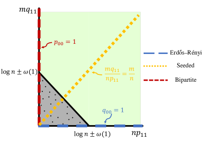
Figure 2: The green region in the figure is information theoretically achievable and the shaded grey region is not achievable. The three lines in the figure represent three specialized settings: the blue line (correlated Erdős–Rényi model) is obtained by setting $q_{00}=1$; the yellow line (seeded Erdős–Rényi model) is obtained by setting $\bm{p}=\bm{q}$; the red line (correlated bipartite model) is obtained by setting $p_{00}=1$. Their intersections with the achievable and not achievable region give the information-theoretic limits of the correlated Erdős–Rényi model, seeded Erdős–Rényi model and the correlated bipartite model separately.

From the information-theoretic limits we derive for the attributed graph pair, we could obtain information-theoretic limits on other existing random graph models as special cases (see Figure 2). Below we highlight how our results, by comparing with the three specialized settings, help answer some of the existing problems in the graph alignment literature. The detailed comparison is given in Section IV.

• Specializing our model by setting $q_{00}=1$, we remove the effect of the attribute vertices and get the correlated Erdős–Rényi graph pair model. Our specialized results recover the information-theoretic limits on Erdős–Rényi graph alignment in [8, 9].

• Specializing our model by setting $\bm{p}=\bm{q}$, we can then treat the $m$ attribute vertices as pre-aligned user vertices and obtain the seeded Erdős–Rényi model. Compared to the best-known information-theoretic limits in [9, 11, 12], our specialized results strictly improves the best-known achievability and converse, establishing the tight threshold for the seeded graph alignment problem in the sparse regime.

• Specializing our model by setting $p_{00}=1$, we remove all of the user-user edges and obtain the correlated bipartite graph pair model. Compared to the best-known information-theoretic limits in [13, 14], our specialized results recover the achievable region for bipartite graph alignment, while strictly improving the converse region.

The main contributions of this paper are summarized as follows.

1. Model Formulation. We propose the attributed Erdős–Rényi pair model, which incorporates both the graph topology similarly and the attribute similarity. Such model formulation allows us to align graphs with the assistance of publicly available side information. Moreover, our model serves as a unifying setting in the graph alignment literature and includes several popular models as its special cases.

2. Information theoretic limits. We establish achievability and converse results on exactly aligning random attributed graphs, where the conditions are tight under assumptions that are typical and interesting in practice. Our results span the full spectrum from the traditional Erdős–Rényi pair model where only the user relationship networks are available to models where only attribute information is available, unifying the existing results in each of these settings. When specialized to the seeded graph alignment and bipartite graph alignment models, our bounds strictly improve the best-known information-theoretic limits for these models.

3. Proof techniques. The proof techniques for the achievability results are mainly inspired by the previous study on Erdős–Rényi graph alignment [9]. For the converse results, we study the phase-transition phenomenon on the existence of indistinguishable vertex pairs, which may be of independent interest.

I-A Related work

The exact graph alignment problem has been studied under various random graph models. One of the most popular random graph models is the correlated Erdős–Rényi pair model $\mathcal{G}(n,\bm{p})$, which generates simple graph pairs without any side information. Under this model, the optimal alignment strategy, derived from the MAP estimator, is enumerating all possible permutations in order to make the two graphs achieve the maximum edge overlap. While the optimal strategy requires exponential time complexity, numerous studies have proposed polynomial-time approaches that exactly solve the graph alignment problem with high probability [15, 16, 17, 18, 19].

Here, we do not attempt to provide further detailed discussions on efficient algorithms, but focus on surveying the information-theoretic limits of exact alignment. Currently, the best-known information-theoretic limits on Erdős–Rényi graph alignment are shown in [9] and [8] by analyzing error event of the MAP estimator. In [9], the authors prove achievability in the regime $n(\sqrt{p_{11}p_{00}}-\sqrt{p_{10}p_{01}})^{2}\geq(2+\epsilon)\log n$. Under certain sparsity conditions, they also show that the achievable region can be improved to $np_{11}\geq\log n+\omega(1)$. In [8], the authors consider a special case of the Erdős–Rényi graph pair model called symmetric subsampling model. In this model, it is assumed that

$$p_{11}=ps^{2},\;p_{01}=p_{10}=ps(1-s),\;p_{00}=1-2ps+ps^{2}$$ (1)

for some $p,s\in[0,1]$. Under this model, the authors prove the achievability in the regime $n(\sqrt{p_{11}p_{00}}-\sqrt{p_{10}p_{01}})^{2}\geq(1+\epsilon)\log n$. For the converse, [9] proves that the permutation cannot be exactly recovered with high probability if $np_{11}\leq\log n-\omega(1)$ by showing the existence of isolated vertices in the intersection graph $G_{1}\wedge G_{2}$. Under the general Erdős–Rényi graph pair model, [8] shows the impossibility of exactly recovering the permutation in the regime $n(\sqrt{p_{11}p_{00}}-\sqrt{p_{10}p_{01}})^{2}\leq(1-\epsilon)\log n$ by showing the existence of permutations that fails the MAP estimator by swapping two vertices. From the aforementioned results, we can see that there is a gap between achievability and converse. Closing this gap is still an open problem.

Recently, there has been a growing interest in studying graph alignment with side information. For example, in the seeded alignment setting, the side information appears in the form of a partial observation of the latent alignment. For the seeded graph alignment problem, there have been a number of studies concentrating on designing polynomial-time algorithms with performance guarantees[20, 21, 11]. Some other more general settings treat any form of side information as vertex attributes and formulate this as the attribute graph alignment problem [22].

There is a line of empirical studies on the attributed graph alignment [23, 22, 24], yet, to the best of our knowledge, there is no known result on information-theoretic limits on graph alignment with attribute information.

II Model

In this section, we describe the attributed Erdős–Rényi graph pair model. Under this model formulation, we formally define the exact attributed graph alignment problem. An illustration of the model is given in Figure 1.

User vertices and attribute vertices. We first generate two graphs, $G_{1}$ and $G_{2}$, on the same vertex set $\mathcal{V}$. The vertex set $\mathcal{V}$ consists of two disjoint sets of vertices, the user vertex set $\mathcal{V}_{\mathrm{u}}$ and the attribute vertex set $\mathcal{V}_{\mathrm{a}}$, i.e., $\mathcal{V}=\mathcal{V}_{\mathrm{u}}\cup\mathcal{V}_{\mathrm{a}}$. Assume that the user vertex set $\mathcal{V}_{\mathrm{u}}$ consists of $n$ vertices, labeled as $[n]\triangleq\{1,2,3,...,n\}$. Assume that the attribute vertex set $\mathcal{V}_{\mathrm{a}}$ consists of $m$ vertices, and $m$ scales as a function of $n$.

Correlated edges. To describe the probabilistic model for edges in $G_{1}$ and $G_{2}$, we first consider the set of user-user vertex pairs $\mathcal{E}_{\mathrm{u}}\triangleq\mathcal{V}_{\mathrm{u}}\times\mathcal{V}_{\mathrm{u}}$ and the set of user-attribute vertex pairs $\mathcal{E}_{\mathrm{a}}\triangleq\mathcal{V}_{\mathrm{u}}\times\mathcal{V}_{\mathrm{a}}$. Then for each vertex pair $e\in\mathcal{E}\triangleq\mathcal{E}_{\mathrm{u}}\cup\mathcal{E}_{\mathrm{a}}$, we write $G_{1}(e)=1$ (resp. $G_{2}(e)=1$) if there is an edge connecting the two vertices in the pair in $G_{1}$ (resp. $G_{2}$), and write $G_{1}(e)=0$ (resp. $G_{2}(e)=0$) otherwise. Since we often consider the same vertex pair in both $G_{1}$ and $G_{2}$, we write $(G_{1},G_{2})(e)$ as a shortened form of $(G_{1}(e),G_{2}(e))$.

The edges of $G_{1}$ and $G_{2}$ are then correlatedly generated in the following way. For each user-user vertex pair $e\in\mathcal{E}_{\mathrm{u}}$, $(G_{1},G_{2})(e)$ follows the joint distribution specified by

$$(G_{1},G_{2})(e)=\begin{cases}(1,1)\;\ \text{w.p.}\;\ p_{11},\\ (1,0)\;\ \text{w.p.}\;\ p_{10},\\ (0,1)\;\ \text{w.p.}\;\ p_{01},\\ (0,0)\;\ \text{w.p.}\;\ p_{00},\end{cases}$$ (2)

where $p_{11},p_{10},p_{01},p_{00}$ are probabilities that sum up to $1$. For each user-attribute vertex pair $e\in\mathcal{E}_{\mathrm{a}}$, $(G_{1},G_{2})(e)$ follows the joint probability distribution specified by

$$(G_{1},G_{2})(e)=\begin{cases}(1,1)\;\ \text{w.p.}\;\ q_{11},\\ (1,0)\;\ \text{w.p.}\;\ q_{10},\\ (0,1)\;\ \text{w.p.}\;\ q_{01},\\ (0,0)\;\ \text{w.p.}\;\ q_{00},\end{cases}$$ (3)

where $q_{11},q_{10},q_{01},q_{00}$ are probabilities that sum up to $1$. The correlation between $G_{1}(e)$ and $G_{2}(e)$ is measured by the correlation coefficient defined as

$$\rho(e) \triangleq\frac{\mathsf{Cov}(G_{1}(e),G_{2}(e))}{\sqrt{\mathsf{Var}[{G_{1}(e)}]}\sqrt{\mathsf{Var}[G_{2}(e)]}},$$

where $\mathsf{Cov}(G_{1}(e),G_{2}(e))$ is the covariance between $G_{1}(e)$ and $G_{2}(e)$ and $\mathsf{Var}[G_{1}(e)]$ and $\mathsf{Var}[G_{2}(e)]$ are the variances. We assume that $G_{1}(e)$ and $G_{2}(e)$ are positively correlated, i,e., $\rho(e)>0$ for every vertex pair $e$. Across different vertex pair $e$’s, the $(G_{1},G_{2})(e)$’s are independent. Finally, recall that there are no edges between attribute vertices in our model.

For compactness of notation, we represent the joint distributions in (2) and (3) in the following matrix form:

$$\bm{p}=\begin{pmatrix}p_{11}&p_{10}\\ p_{01}&p_{00}\end{pmatrix}\quad\text{ and }\quad\bm{q}=\begin{pmatrix}q_{11}&q_{10}\\ q_{01}&q_{00}\end{pmatrix}.$$

We refer to the graph pair $(G_{1},G_{2})$ as an attributed Erdős–Rényi pair $\mathcal{G}(n,\bm{p},m,\bm{q})$. Note that this model is equivalent to the subsampling model in the literature [6].

Anonymization and exact alignment. In the attributed graph alignment problem, we are given $G_{1}$ and an anonymized version of $G_{2}$, denoted as $G_{2}^{\prime}$. The anonymized graph $G_{2}^{\prime}$ is generated by applying a random permutation $\Pi^{*}$ on the user vertex set of $G_{2}$, where the permutation $\Pi^{*}$ is unknown. More explicitly, each user vertex $i$ in $G_{2}$ is re-labeled as $\Pi^{*}(i)$ in $G_{2}^{\prime}$. The permutation $\Pi^{*}$ is chosen uniformly at random from $\mathcal{S}_{n}$, where $\mathcal{S}_{n}$ is the set of all permutations on $[n]$. Since $G_{1}$ and $G_{2}^{\prime}$ are observable, we refer to $(G_{1},G_{2}^{\prime})$ as the observable pair generated from the attributed Erdős–Rényi pair $\mathcal{G}(n,\bm{p},m,\bm{q})$.

Then the graph alignment problem, i.e., the problem of recovering the identities/original labels of user vertices in the anonymized graph $G_{2}^{\prime}$, can be formulated as a problem of estimating the underlying permutation $\Pi^{*}$. The goal of graph alignment is to design an estimator $\hat{\pi}(G_{1},G_{2}^{\prime})$ as a function of $G_{1}$ and $G_{2}^{\prime}$ to best estimate $\Pi^{*}$. We say $\hat{\pi}(G_{1},G_{2}^{\prime})$ achieves exact alignment if $\hat{\pi}(G_{1},G_{2}^{\prime})=\Pi^{*}$. The probability of error for exact alignment is defined as $\mathsf{P}(\hat{\pi}(G_{1},G_{2}^{\prime})\neq\Pi^{*})$. We say exact alignment is achievable with high probability (w.h.p.) if there exists $\hat{\pi}$ such that $\lim_{n\to\infty}\mathsf{P}(\hat{\pi}(G_{1},G_{2}^{\prime})\neq\Pi^{*})=0.$

Reminder of the Landau notation.

Notation	Definition
$f(n)=\omega(g(n))$	$\lim\limits_{n\rightarrow\infty}\frac{|f(n)|}{g(n)}=\infty$
$f(n)=o(g(n))$	$\lim\limits_{n\to\infty}\frac{|f(n)|}{g(n)}=0$
$f(n)=O(g(n))$	$\limsup\limits_{n\rightarrow\infty}\frac{|f(n)|}{g(n)}<\infty$
$f(n)=\Omega(g(n))$	$\liminf\limits_{n\rightarrow\infty}\frac{|f(n)|}{g(n)}>0$
$f(n)=\Theta(g(n))$	$f(n)=O(g(n))$ and $f(n)=\Omega(g(n))$

III Main results

In this section, we state the achievability results (Theorem 1 and Theorem 2) and the converse result (Theorem 3). To better demonstrate the benefit from attribute information, we also present a simplified version of the results under some mild and practical assumptions as Corollary 1.

Throughout the remainder of the paper, we define

$$\psi_{\mathrm{u}} \triangleq(\sqrt{p_{11}p_{00}}-\sqrt{p_{10}p_{01}})^{2}$$ (4)

$$\psi_{\mathrm{a}} \triangleq(\sqrt{q_{11}q_{00}}-\sqrt{q_{10}q_{01}})^{2}.$$ (5)

Theorem 1 (General achievability).

Consider the attributed Erdős–Rényi pair $\mathcal{G}(n,\bm{p};m,\bm{q})$. If

$$\tfrac{1}{2}n\psi_{\mathrm{u}}+m\psi_{\mathrm{a}}-\log{n}=\omega(1),$$ (6)

then the MAP estimator achieves exact alignment w.h.p.

Theorem 2 (Achievability in sparse region).

Consider the attributed Erdős–Rényi pair $\mathcal{G}(n,\bm{p};m,\bm{q})$. If

$$p_{11} =O\left(\tfrac{\log{n}}{n}\right),$$ (7)

$$p_{10}+p_{01} =O\left(\tfrac{1}{\log{n}}\right),$$ (8)

$$\frac{p_{10}p_{01}}{p_{11}p_{00}} =O\left(\tfrac{1}{(\log{n})^{3}}\right),$$ (9)

$$np_{11}+m\psi_{\mathrm{a}}-\log{n} =\omega(1),$$ (10)

then the MAP estimator achieves exact alignment w.h.p.

Theorem 3 (Converse).

Consider the attributed Erdős–Rényi pair $\mathcal{G}(n,\bm{p};m,\bm{q})$. If

$$np_{11}+mq_{11}-\log{n}\rightarrow-\infty,$$ (11)

then no algorithm guarantees exact alignment w.h.p.

To better illustrate the benefit of attribute information in the graph alignment problem, we present in Corollary 1 a simplified version of our achievability result by adding mild assumptions on user-user edges motivated by practical applications. In addition, this simplified result makes it easier to compare the achievability result to the converse result in Theorem 3, which will be illustrated in Figure 2. Note that these additional assumptions are not needed for technical proofs.

In a typical social network, the degree of a vertex is much smaller than the total number of users. Based on this observation, we assume that the marginal probabilities of an edge in both $G_{1}$ and $G_{2}$ are not going to 1, i.e.,

$$1-(p_{11}+p_{10})=\Theta(1),\;\ 1-(p_{11}+p_{01})=\Theta(1),$$ (12)

$$1-(q_{11}+q_{10})=\Theta(1),\;\ 1-(q_{11}+q_{01})=\Theta(1).$$ (13)

Moreover, two social networks on the same set of users are typically highly correlated. Based on this, we assume that the correlation coefficient of user-user and user-attribute edges, denoted as $\rho_{\mathrm{u}}$ and $\rho_{\mathrm{a}}$, are not vanishing, i.e.,

$$\rho_{\mathrm{u}}=\Theta(1),\;\ \rho_{\mathrm{a}}=\Theta(1).$$ (14)

Corollary 1 (Simplified achievability).

Consider the attributed Erdős–Rényi pair $\mathcal{G}(n,\bm{p};m,\bm{q})$ under conditions (12) and (14). If

$$np_{11}+m\psi_{\mathrm{a}}-\log{n}\rightarrow\infty,$$ (15)

then the MAP estimator achieves exact alignment w.h.p.

If, in addition, condition (13) is satisfied, then condition (15) simplifies to

$$np_{11}+mq_{11}-\log{n}\rightarrow\infty, m=\Omega((\log{n})^{3}),$$ if (16)

$$np_{11}+mq_{11}-ma_{n}-\log{n}\rightarrow\infty, m=o((\log{n})^{3}),$$ if (17)

where $a_{n}=q_{11}-\psi_{\mathrm{a}}=O(q_{11}^{3/2})$.

The proof of Corollary 1 can be found in Appendix E. Here, we visualize this simplified achievability result together with the our converse result in Figure 3. The gap between the achievability and the converse comes from the difference between $mq_{11}$ and $m\psi_{\mathrm{a}}$. In particular, we show the matching achievability and converse results (Figure 2) when $m=\Omega((\log n)^{3})$. How to the gap in case $m=o((\log n)^{3})$ is an open problem.

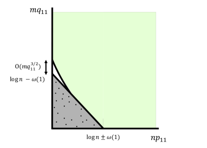
Figure 3: The green region is information theoretically achievable and is specified by condition (17); the shaded grey region in not achievable according the Theorem 3. The gap between the achievability and converse represent $q_{11}-\psi_{\mathrm{a}}=O(q_{11}^{3/2})$. In particular, this gap is negligible up to $\pm\omega(1)$ when $m=\Omega((\log n)^{3})$, which is the special case presented in Figure 2.

IV Comparison

In this section, we specialize our main results (Theorems 1,  2, and 3) on exact alignment of the attributed Erdős–Rényi pair model to three closely related graph alignment problems: the Erdős–Rényi graph alignment, the seeded Erdős–Rényi graph alignment, and the bipartite graph alignment. We compare them with the best-known results in the literature.

IV-A Erdős–Rényi graph pair

The correlated Erdős–Rényi pair model $\mathcal{G}(n,\bm{p})$ is the setting most commonly studied for graph alignment tasks that consider only graph topology similarity [6, 7, 8, 9, 15]. This model generates graph pairs that contain only user vertices. For a pair of graphs $G_{1}$, $G_{2}$ obtained from this model $\mathcal{G}(n,\bm{p})$, we use $\mathcal{V}_{\mathrm{u}}$ to denote their vertex set and $|\mathcal{V}_{\mathrm{u}}|=n$. The edges in $G_{1}$ and $G_{2}$ are generated jointly in the following way: for a pair of users $e\in{\mathcal{V}_{\mathrm{u}}\choose 2}$, we have

$$(G_{1},G_{2})(e)=\begin{cases}(1,1)\;\ \text{w.p.}\;\ p_{11},\\ (1,0)\;\ \text{w.p.}\;\ p_{10},\\ (0,1)\;\ \text{w.p.}\;\ p_{01},\\ (0,0)\;\ \text{w.p.}\;\ p_{00}.\end{cases}$$ (18)

The anonymized graph $G_{2}^{\prime}$ is obtained by applying a random permutation $\Pi^{*}$ on the vertices of $G_{2}$. This model can be specialized from the attributed graph pair model by setting the number of attributes $m=0$ or $q_{00}=1$. For aligning the correlated Erdős–Rényi pair, the best-known information-theoretic limits are established in [8, 9] and we state the combined results here for ease of comparison.

Theorem 4 (Best-known information theoretic limits [8, 9]).

Consider the correlated Erdős–Rényi pair $\mathcal{G}(n,\bm{p})$.
Achievability:
If

$$n\psi_{\mathrm{u}}\geq 2\log n+\omega(1),$$ (19)

or

$$p_{11} =O\left(\tfrac{1}{\log{n}}\right),$$ (20)

$$p_{10}+p_{01} =O\left(\tfrac{1}{\log{n}}\right),$$ (21)

$$\frac{p_{10}p_{01}}{p_{11}p_{00}} =O\left(\tfrac{1}{(\log{n})^{3}}\right),$$ (22)

$$np_{11} =\log{n}+\omega(1),$$ (23)

then the MAP estimator achieves exact alignment w.h.p.
Converse:
If there exist a constant $\epsilon\in(0,1)$ such that

$$n\psi_{\mathrm{u}}\leq(1-\epsilon)\log n,$$ (24)

or

$$np_{11}\leq\log n-\omega(1),$$ (25)

then no algorithm guarantees exact alignment w.h.p.

Remark 1.

We point out that in the dense regime, i.e., at least one of conditions (20), (21) and (22) is not satisfied, Theorem 4 in [8] provides a tighter achievability result. However, as we mentioned in the introduction, the result is limited to the symmetric subsampling model (1). In this section, we focus on the comparison under the general Erdős–Rényi pair model, so the result from Theorem 4 in [8] is not listed as one of the best known information theoretic limit. On the other hand, the converse result in [8] is not limited to the symmetric subsampling model. Thus, we include the result as equation (24) in Theorem 4.

We now specialize the attributed Erdős–Rényi pair model to the correlated Erdős–Rényi pair by setting $q_{00}=1$. Theorems 1,  2, and 3 simplify to the following.

Theorem 5 (Specialization from attributed Erdős–Rényi pair).

Consider the attributed Erdős–Rényi pair $\mathcal{G}(n,\bm{p};m,\bm{q})$ with $q_{00}=1$.
Achievability:
If

$$n\psi_{\mathrm{u}}\geq 2\log n+\omega(1),$$ (26)

or

$$p_{11} =O\left(\tfrac{\log{n}}{n}\right),$$ (27)

$$p_{10}+p_{01} =O\left(\tfrac{1}{\log{n}}\right),$$ (28)

$$\frac{p_{10}p_{01}}{p_{11}p_{00}} =O\left(\tfrac{1}{(\log{n})^{3}}\right),$$ (29)

$$np_{11} =\log{n}+\omega(1),$$ (30)

then the MAP estimator achieves exact alignment w.h.p.
Converse: If

$$np_{11}\leq\log n-\omega(1),$$

then no algorithm guarantees exact alignment w.h.p.

Remark 2.

When specialized to the Erdős–Rényi pair model, our achievability result recovers the best-known achievability result from [8, 9], while our converse result is a strict subset of that given by conditions (24) and (25). To see the achievability results in Theorems 4 and 5 are equivalent, we observe that the difference between the region characterized by (20)–(23) and the region characterized by (27)–(30) is given by $p_{11}=\omega(\frac{\log n}{n})$ and $p_{11}=O(\frac{1}{\log n}).$ However, under the assumptions (28) and (29), we know that $p_{00}=1-o(1)$ and $\frac{p_{10}p_{01}}{p_{00}p_{11}}=o(1)$. If $p_{11}=\omega(\frac{\log n}{n})$, then these further imply that $\psi_{\mathrm{u}}=(1+o(1))p_{11}p_{00}=\omega(\frac{\log n}{n})$, i.e., the difference between the two regions falls in the achievable region characterized by (26). Thus, the achievability region in Theorem 5 is exactly the same as that in Theorem 4. For the converse, it is an open question whether a converse result for the attributed Erdős–Rényi pair model can be established, which recovers condition (24) when specialized to the Erdős–Rényi pair model.

IV-B Seeded Erdős–Rényi graph pair

In the seeded graph model $\mathcal{G}(n,m,\bm{p})$, a pair of graphs $G_{1},G_{2}$ are generated from the correlated Erdős–Rényi pair model $\mathcal{G}(n+m,\bm{p})$. Then the anonymized graph $G_{2}^{\prime}$ is obtained by applying a random permutation on the vertices of $G_{2}$. In addition to knowing $G_{1}$ and $G_{2}^{\prime}$, in the seeded graph setting, we are also given the true alignment on a set of the user vertices, which is known as the seed set $\mathcal{V}_{s}$. The number of aligned pairs in $\mathcal{V}_{s}$ is a fixed number $m$. The seeded alignment problem has been studied by [5, 11, 25, 20, 26]. Moreover, achievability results on unseeded graph alignment problem also trivially imply achievability results on seeded graph alignment problem. To the best of our knowledge, the best information-theoretic limits of the seeded alignment problem are given by [9, 11, 12]. For the simplicity of our discussion, we focus only on the symmetric subsampling model (1) with sparsity conditions

$$p=O\left(\frac{1}{(\log n)^{3}}\right)\text{ and }s=\Theta(1).$$ (31)

Theorem 6 (Best-known information-theoretic limits in the sparse and symmetric regime [9, 11, 12]).

Consider the seeded Erdős–Rényi graph pair $\mathcal{G}(n,m,\bm{p})$ satisfying conditions (1) and (31).
Achievability from [9]: Assume

$$(n+m)p_{11}=\log(n+m)+\omega(1).$$ (32)

Then the unseeded MAP estimator achieves exact alignment w.h.p.
Achievability from [12]:

1. In the regime where $mp_{11}=\Omega(\log n)$, if for a constant $\epsilon>0$, we have

   $$(n+m)p_{11}\geq(1+\epsilon)\log n,$$ (33)

   then the AttrRich algorithm in [12] achieves exact alignment w.h.p.

2. In the regime where $mp_{11}=o(\log n)$, if for a constant $\tau>0$, we have

   $$np_{11} =\log n+\omega(1),$$ (34)

   $$mp_{11} \geq\frac{2\log n}{\tau\log(p_{11}/(p_{11}+p_{10})^{2})},$$ (35)

   then the AttrSparse algorithm in [12] achieves exact alignment w.h.p.

Converse from [11] Consider the seeded Erdős–Rényi graph pair $\mathcal{G}(n,m,\bm{p})$. If

$$(n+m)p_{11}\leq\log{(n+m)}+O(1)\;\ \text{and}\;\ m=O(n),$$

then no algorithm achieves exact recovery w.h.p.

To compare the best-known information-theoretic limits of the seeded Erdős–Rényi alignment with our results, we specialize the attributed Erdős–Rényi pair model by setting $\bm{p}=\bm{q}$, where $m$ attribute vertices are pre-aligned seeds. Notice that a small difference between the $\mathcal{G}(n,\bm{p};m,\bm{p})$ model and the seeded model $\mathcal{G}(n,m,\bm{p})$ is that there are no edges between the seeds in the specialized model but those edges exist in the seeded model. Such distinction may lead to a difference in the design of seeded graph alignment algorithms (e.g. algorithms from [11] exploit seed-seed edges). It turns out that such seed-seed edges have no influence on the optimal MAP estimators for the two models, which leads to the next lemma.

Lemma 1.

The information-theoretic limits on exact alignment in the seeded Erdős–Rényi pair model $\mathcal{G}(n,m,\bm{p})$ and the information-theoretic limits on exact alignment in the specialized attributed Erdős–Rényi pair model $\mathcal{G}(n,\bm{p};m,\bm{p})$ are identical.

Proof.

See Appendix B. ∎

Based on Lemma 1, we directly obtain the achievability and converse results on seeded graph alignment from Theorems 1, 2, and 3 by setting $\bm{p}=\bm{q}$. The specialized achievability and converse results strictly improve the best known achievability and converse in the literature for seeded graph alignment.

Theorem 7 (Specialization from attributed Erdős–Rényi pair).

Consider the attributed Erdős–Rényi pair $\mathcal{G}(n,\bm{p};m,\bm{p})$.
Achievability:
If

$$(n+m)\psi_{\mathrm{u}}\geq 2\log n+\omega(1),$$ (36)

or

$$p_{11} =O\left(\tfrac{\log{n}}{n}\right),$$ (37)

$$p_{10}+p_{01} =O\left(\tfrac{1}{\log{n}}\right),$$ (38)

$$\frac{p_{10}p_{01}}{p_{11}p_{00}} =O\left(\tfrac{1}{(\log{n})^{3}}\right),$$ (39)

$$np_{11}+m\psi_{\mathrm{u}} =\log{n}+\omega(1),$$ (40)

then the MAP estimator achieves exact alignment w.h.p.
Converse:
If

$$(n+m)p_{11}\leq\log n-\omega(1),$$

then no algorithm guarantees exact alignment w.h.p.

Moreover, if the two seeded graphs $G_{1}$ and $G_{2}^{\prime}$ satisfy the two assumptions on typical social networks (see Section III), then we have the following matching achievability and converse results.

Corollary 2 (Threshold for sparse seeded Erdős–Rényi pair).

Consider the seeded Erdős–Rényi pair model $\mathcal{G}(n,m,\bm{p})$ under conditions (12) and (14).
Achievability: If

$$(n+m)p_{11}\geq\log{n}+\omega(1),$$ (41)

then the MAP estimator achieves exact alignment w.h.p.
Converse: If

$$(n+m)p_{11}\leq\log{n}-\omega(1),$$ (42)

then no algorithm guarantees exact alignment w.h.p.

Proof.

See Appendix F. ∎

Remark 3.

The sparse symmetric subsampling model conditions (1) and (31) together imply conditions (12) and (14). In Corollary 2, we obtain asymptotically tight achievability and converse under the sparse symmetric subsampling model.

Remark 4 (Comparison between achievability results).

The achievability result in Corollary 2 strictly improves the best-known achievability results for seeded alignment [9, 12]. In the following, we present an example which is in the achievable region of Corollary 2, but not in the achievable region of Theorem 6. Consider the sparse symmetric subsampling model satisfying (1) and (31). Assume that

$$m=n^{2},\;p_{11}=\frac{\log n+\log\log n}{m+n},\text{ and }p_{01}=p_{10}=0.$$

We see that condition (41) holds because $(n+m)p_{11}=\log n+\log\log n=\log n+\omega(1)$. Moreover, we have $1-(p_{11}+p_{01})=1-(p_{11}+p_{10})=1-\frac{\log n+\log\log n}{n^{2}+n}=\Theta(1)$ and $\rho_{\rm{u}}=\rho_{\rm{a}}=1$, satisfying conditions (12) and (14). However, condition (32) $(n+m)p_{11}=\log(n+m)+\omega(1)$ in Theorem 6 does not hold because $(n+m)p_{11}<2\log n<\log(n+m)+\omega(1)$, and condition (33) $(n+m)p_{11}\geq(1+\epsilon)\log n$ in Theorem 6 does not hold because $(n+m)p_{11}=\log n+\log\log n<(1+\epsilon)\log n$ for any positive constant $\epsilon$. So this example lies in the achievable region of Corollary 2, but not in that of Theorem 6.

Remark 5 (Comparison between converse results).

Our converse result in Corollary 2 strictly improves the best-known converse result in [11]. To see this, here we first simplify the converse result from Theorem 6. Note that under the condition $m=O(n)$, we have $\log{(n+m)}=\log{n}+O(1)$. Therefore, the converse condition in Theorem 6 is equivalent to

$$(n+m)p_{11}\leq\log{n}+O(1),\;\ \text{and}\;\ m=O(n).$$

Then we can directly see that in the regime $m=O(n)$, our specialized converse condition $(n+m)p_{11}\leq\log{n}-\omega(1)$ implies the converse in Theorem 6. However, in the $m=\omega(n)$ regime, Theorem 6 does not provide a condition for converse, while our converse condition is still valid when $m=\omega(n)$.

IV-C Bipartite graph pair

In the bipartite graph pair model $\mathcal{G}(n,m,\bm{q})$, each graph is a bipartite graph on two disjoint set of vertices, i.e., the user vertex set $\mathcal{V}_{\mathrm{u}}$ and attribute vertex set $\mathcal{V}_{\mathrm{a}}$. The edges between the two set of vertices are generated in a correlated way: for $e\in\mathcal{V}_{\mathrm{u}}\times\mathcal{V}_{\mathrm{a}}$

$$(G_{1},G_{2})(e)=\begin{cases}(1,1)\;\ \text{w.p.}\;\ q_{11},\\ (1,0)\;\ \text{w.p.}\;\ q_{10},\\ (0,1)\;\ \text{w.p.}\;\ q_{01},\\ (0,0)\;\ \text{w.p.}\;\ q_{00}.\end{cases}$$ (43)

The anonymized graph $G_{2}^{\prime}$ is obtained by applying a random permutation $\Pi^{*}$ only on the user vertex set of $G_{2}$. Aligning such correlated bipartite graph is also known as a special case of the database alignment problem [27]. The best-known information-theoretic limits of database alignment are studied in [27]. We restate the achievability and converse results from [27] when specialized to the case of bipartite graph pair alignment in Theorem 8.

Theorem 8 (Best-known information-theoretic limits [27]).

Consider the bipartite graph pair model $\mathcal{G}(n,m,\bm{q})$.
Achievability:
If

$$-\frac{m}{2}\log(1-2\psi_{\mathrm{a}})\geq\log n+\omega(1),$$ (44)

then there exists an estimator that achieves exact alignment w.h.p.
Converse:
If

$$-\frac{m}{2}\log(1-2\psi_{\mathrm{a}})\leq(1-\Omega(1))\log n,$$ (45)

then no estimator achieves exact alignment w.h.p.

Remark 6.

In [27], the left-hand side of both inequalities in Theorem 8 are stated in a different, yet equivalent, form. To state it, we need to introduce two definitions. Let $A=\begin{pmatrix}A_{00}&A_{01}\\ A_{10}&A_{11}\end{pmatrix}$ be a $2\times 2$ probability matrix with all non-negative entries and $A_{00}+A_{01}+A_{10}+A_{11}=1$. We define $A^{\otimes k}$ to be a $2^{k}\times 2^{k}$ probability matrix with rows and columns both indexed by $\{0,1\}^{k}$, and for $a,b\in\{0,1\}^{k}$, we have $A^{\otimes k}_{a,b}=\Pi_{i=1}^{k}A_{a_{i},b_{i}}$. Matrix $A^{\otimes k}$ is called the $k$th tensor product of $A$. For a probability matrix $A$ and an integer $l\geq 2$, we define the order-$l$ cycle mutual information of $A$ to be $I_{l}^{\circ}(A)=\frac{1}{1-l}\log\mathrm{tr}((ZZ^{T})^{l})$, where $Z$ is a matrix with same dimension as $A$ and $Z_{ij}=\sqrt{A_{ij}}$ for any index pair $(i,j)$. In [27], the left-hand side of both inequalities are given as $\frac{1}{2}I^{\circ}_{2}(Q^{\otimes m})$, where $Q=\begin{pmatrix}q_{00}&q_{01}\\ q_{10}&q_{11}\end{pmatrix}$. According to [27], the cycle mutual information satisfies a nice property that $I^{\circ}_{2}(Q^{\otimes m})=mI^{\circ}_{2}(Q)$. Furthermore, we can calculate the $2$-cycle mutual information of $Q$ as $I^{\circ}_{2}(Q)=-\log(1-2\psi_{\mathrm{a}})$, which implies that $\frac{1}{2}I^{\circ}_{2}(Q^{\otimes m})=-\frac{m}{2}\log(1-2\psi_{\mathrm{a}})$.

To compare our results with the best-known database alignment information-theoretic limits, we specialize the attributed Erdős–Rényi pair model to the bipartite graph pair by removing all of the edges between user vertices, i.e., $p_{00}=1$. Correspondingly, we obtain the following achievable and converse result on bipartite graph alignment from Theorems 1 and 3.

Theorem 9 (Specialization from attributed Erdős–Rényi pair).

Consider the attributed Erdős–Rényi pair $\mathcal{G}(n,\bm{p};m,\bm{q})$ with $p_{00}=1$.
Achievability:
If

$$m\psi_{\mathrm{a}}\geq\log n+\omega(1),$$ (46)

then the MAP estimator achieves exact alignment w.h.p.
Converse:
If

$$mq_{11}\leq\log n-\omega(1),$$ (47)

then no algorithm guarantees exact alignment w.h.p.

Remark 7.

The achievable region in Theorem 9 is a strict subset of the achievable region in Theorem 8. This because $-\frac{m}{2}\log(1-2\psi_{\mathrm{a}})>m\psi_{\mathrm{a}}$. However, in the derivation steps (67)–(69) of Theorem 1, we were replacing the logarithm term by applying $\log(1+x)\leq x$. Without this step of loosening the bound, equation (46) can be replaced by $-\frac{m}{2}\log(1-2\psi_{\mathrm{a}})\geq\log n+\omega(1)$, which is the same as equation (44). Therefore, although the achievability region (46) in Theorem 9 does not directly recover the achievable region (44) in Theorem 8, it can be improved to the achievable region (44) by a slight modification of derivations steps (67)–(69).

Remark 8 (Comparison between converse regions).

The converse region (47) in Theorem 9 strictly improves the best known converse region for bipartite alignment (45) in Theorem 8. To show the strict improvement, consider an instance of the parameters satisfying $q_{11}=\frac{\log n-\log\log n}{m}$, $q_{00}=1-q_{11}$, $q_{01}=q_{10}=0$ and $m=\omega(\log n)$. Because $mq_{11}=\log n-\log\log n\leq\log n-\omega(1)$, this instance of parameters is in the converse region given by (47). However, this instance is out of the converse region (45), because

$$-\frac{m}{2}\log(1-2\psi_{\mathrm{a}}) =-\frac{m}{2}\log(1-2(\sqrt{q_{11}q_{00}}-\sqrt{q_{01}q_{10}})^{2})$$

$$=-\frac{m}{2}\log(1-2q_{00}q_{11})$$

$$\geq\frac{m}{2}2q_{00}q_{11}$$

$$=(\log n-\log\log n)(1-o(1))$$

$$>(1-\Omega(1))\log n.$$

V Proof of converse statement

In this section, we give a detailed proof for Theorem 3. Let $(G_{1},G_{2})$ be an attributed Erdős–Rényi pair $\mathcal{G}(n,\bm{p};m,\bm{q})$. In this proof, we will focus on the intersection graph of $G_{1}$ and $G_{2}$, denoted as $G_{1}\wedge G_{2}$, which is the graph on the vertex set $\mathcal{V}=\mathcal{V}_{\mathrm{u}}\cup\mathcal{V}_{\mathrm{a}}$ whose edge set is the intersection of the edge sets of $G_{1}$ and $G_{2}$. We say a permutation $\pi$ on the vertex set $\mathcal{V}$ is an automorphism of $G_{1}\wedge G_{2}$ if a vertex pair $(i,j)$ is in the edge set of $G_{1}\wedge G_{2}$ if and only if $(\pi(i),\pi(j))$ is in the edge set of $G_{1}\wedge G_{2}$, i.e., if $\pi$ is edge-preserving. Note that an identity permutation is always an automorphism. Let $\mathrm{Aut}(G_{1}\wedge G_{2})$ denote the set of automorphisms of $G_{1}\wedge G_{2}$. By Lemma 2 below, exact alignment cannot be achieved w.h.p. if $\mathrm{Aut}(G_{1}\wedge G_{2})$ contains permutations other than the identity permutation. This allows us to establish conditions for not achieving exact alignment w.h.p. by analyzing automorphisms of $G_{1}\wedge G_{2}$.

Lemma 2 ([7]).

Let $(G_{1},G_{2})$ be an attributed Erdős–Rényi pair $\mathcal{G}(n,\bm{p};m,\bm{q})$. Given $|\mathrm{Aut}(G_{1}\wedge G_{2})|$, the probability that MAP estimator succeeds is at most $\frac{1}{|\mathrm{Aut}(G_{1}\wedge G_{2})|}$.

In the proof of Theorem 3, we will further focus on the automorphisms given by swapping two user vertices. To this end, we first define the following equivalence relation between a pair of user vertices. We say two user vertices $i$ and $j$ ($i\neq j$) are indistinguishable in $G_{1}\wedge G_{2}$, denoted as $i\equiv j$, if $(G_{1}\wedge G_{2})((i,v))=(G_{1}\wedge G_{2})((j,v))$ for all $v\in\mathcal{V}$. It is not hard to see that swapping two indistinguishable vertices is an automorphism of $G_{1}\wedge G_{2}$, and thus $|\mathrm{Aut}(G_{1}\wedge G_{2})\setminus\{\textrm{identity permutation}\}|\geq|\{\textrm{indistinguishable vertex pairs}\}|$. Therefore, in the proof below, we show that the number of such indistinguishable vertex pairs is positive with a large probability, which suffices for proving Theorem 3.

See 3

Proof of Theorem 3.

Let $G_{1}$ and $G_{2}$ be an attributed Erdős–Rényi pair $\mathcal{G}(n,\bm{p};m,\bm{q})$ and let $G=G_{1}\wedge G_{2}$. Let $X$ denote the number of indistinguishable user vertex pairs in $G$, i.e.,

$$X=\sum_{i<j\colon i,j\in\mathcal{V}_{\mathrm{u}}}\mathbb{1}\{i\equiv j\}.$$

We will show that $\mathsf{P}(X=0)\to 0$ as $n\to\infty$ if the condition (11) in Theorem 3 is satisfied.

We start by upper-bounding $\mathsf{P}(X=0)$ using Chebyshev’s inequality

$$\mathsf{P}(X=0)\leq\frac{\mathsf{Var}(X)}{\mathsf{E}[X]^{2}}=\frac{\mathsf{E}[X^{2}]-\mathsf{E}[X]^{2}}{\mathsf{E}[X]^{2}}.$$ (48)

For the first moment term $\mathsf{E}[X]$, we have

$$\mathsf{E}[X]=\sum_{i<j}\mathsf{P}(i\equiv j)={n\choose 2}\mathsf{P}(i\equiv j).$$ (49)

For the second moment term $\mathsf{E}[X^{2}]$, we expand the sum as

$$\mathsf{E}[X^{2}] =\mathsf{E}\Biggl{[}\sum_{i<j}\mathbb{1}\{i\equiv j\}\cdot\sum_{k<l}\mathbb{1}\{k\equiv l\}\Biggr{]}$$

$$=\mathsf{E}\Biggl{[}\sum_{i<j}\mathbb{1}\{i\equiv j\}+\mspace{-12.0mu}\sum_{\begin{subarray}{c}i,j,k,l\colon i<j,k<l\\ i,j,k,l\textrm{ are distinct}\end{subarray}}\mathbb{1}\{i\equiv j\}\cdot\mathbb{1}\{k\equiv l\}$$

$$\mspace{48.0mu}+\mspace{-12.0mu}\sum_{\begin{subarray}{c}i,j,k,l\colon i<j,k<l\\ \textrm{$\{i,j\}$ and $\{k,l\}$ share one element}\end{subarray}}\mspace{-24.0mu}\mathbb{1}\{i\equiv j\equiv k\equiv l\}\Biggr{]}$$

$$={n\choose 2}\mathsf{P}(i\equiv j)+{n\choose 4}{4\choose 2}\mathsf{P}(i\equiv j\text{ and }k\equiv l)$$

$$\mspace{23.0mu}+6{n\choose 3}\mathsf{P}(i\equiv j\equiv k),$$ (50)

where $i,j,k,l$ are distinct in (50). With (49) and (50), the upper bound given by Chebyshev’s inequality in (48) can be written as

$$\frac{\mathsf{Var}(X)}{\mathsf{E}[X]^{2}} =\frac{2}{n(n-1)\mathsf{P}(i\equiv j)}+\frac{4(n-2)}{n(n-1)}\frac{\mathsf{P}(i\equiv j\equiv k)}{\mathsf{P}(i\equiv j)^{2}}$$

$$\mspace{23.0mu}+\frac{(n-2)(n-3)}{n(n-1)}\frac{\mathsf{P}(i\equiv j\text{ and }k\equiv l)}{\mathsf{P}(i\equiv j)^{2}}-1.$$ (51)

To compute $\mathsf{P}(i\equiv j)$, we look into the event $\{i\equiv j\}$ which is the intersection of $A_{1}$ and $A_{2}$, where $A_{1}=\{\forall v\in\mathcal{V}_{\mathrm{u}}\setminus\{i,j\},\,G((i,v))=G((j,v))\}$, and $A_{2}=\{\forall u\in\mathcal{V}_{\mathrm{a}},\,G((i,u))=G((j,u))\}$. Recall that in the intersection graph $G=G_{1}\wedge G_{2}$, the edge probability is $p_{11}$ for user-user pairs and $q_{11}$ for user-attribute pairs. Therefore,

$$\mathsf{P}(A_{1}) =\sum_{i=0}^{n-2}{n-2\choose i}p_{11}^{2i}(1-p_{11})^{2(n-2-i)}$$

$$=\left(p_{11}^{2}+(1-p_{11})^{2}\right)^{n-2},$$

$$\mathsf{P}(A_{2}) =\sum_{i=0}^{m}{m\choose i}p_{11}^{2i}(1-p_{11})^{2(m-i)}$$

$$=\left(q_{11}^{2}+(1-q_{11})^{2}\right)^{m}.$$

Since $A_{1}$ and $A_{2}$ are independent, we have

$$\mspace{23.0mu}\mathsf{P}(i\equiv j)$$ (52)

$$=\mathsf{P}(A_{1})\mathsf{P}(A_{2})$$

$$=\left(p_{11}^{2}+(1-p_{11})^{2}\right)^{n-2}\left(q_{11}^{2}+(1-q_{11})^{2}\right)^{m}$$

$$=\left(1-2p_{11}+2p_{11}^{2}\right)^{n-2}\left(1-2q_{11}+2q_{11}^{2}\right)^{m}.$$ (53)

Similarly, to compute $\mathsf{P}(i\equiv j\equiv k)$, we look into the event $\{i\equiv j\equiv k\}$ which is the intersection of events $B_{0}$, $B_{1}$ and $B_{2}$, where $B_{0}=\{G((i,j))=G((j,k))=G((i,k))\}$, $B_{1}=\{\forall v\in\mathcal{V}_{\mathrm{u}}\setminus\{i,j,k\},\,G((i,v))=G((j,v))=G((k,v))\}$, and $B_{2}=\{\forall u\in\mathcal{V}_{\mathrm{a}},\,G((i,u))=G((j,u))=G((k,u))\}$. Then, the probabilities of those three events are

$$\mathsf{P}(B_{0})=p_{11}^{3}+(1-p_{11})^{3},$$

$$\mathsf{P}(B_{1})=\left(p_{11}^{3}+(1-p_{11})^{3}\right)^{n-3},$$

$$\mathsf{P}(B_{2})=\left(q_{11}^{3}+(1-q_{11})^{3}\right)^{m}.$$

Since the events $B_{0}$, $B_{1}$ and $B_{2}$ are independent, we have

$$\mspace{23.0mu}\mathsf{P}(i\equiv j\equiv k)$$

$$=\mathsf{P}(B_{0})\mathsf{P}(B_{1})\mathsf{P}(B_{2})$$

$$=\left(p_{11}^{3}+(1-p_{11})^{3}\right)^{n-2}\left(q_{11}^{3}+(1-q_{11})^{3}\right)^{m}$$

$$=(1-3p_{11}+3p_{11}^{2})^{n-2}(1-3q_{11}+3q_{11}^{2})^{m}.$$

To compute $\mathsf{P}(i\equiv j\text{ and }k\equiv l)$, we look into the event $\{i\equiv j\text{ and }k\equiv l\}$ which is the intersection of $C_{0}$, $C_{1}$, $C_{1}^{\prime}$, $C_{2}$ and $C_{2}^{\prime}$, where $C_{0}=\{G(i,k)=G(j,k)=G(i,l)=G(j,l)\}$, $C_{1}=\{\forall v\in\mathcal{V}_{\mathrm{u}}\setminus\{i,j,k,l\},G(i,v)=G(j,v)\}$, $C_{1}^{\prime}=\{\forall v\in\mathcal{V}_{\mathrm{u}}\setminus\{i,j,k,l\},G(k,v)=G(l,v)\}$, $C_{2}=\{\forall u\in\mathcal{V}_{\mathrm{a}},G(i,u)=G(j,u)\}$ and $C_{2}^{\prime}=\{\forall u\in\mathcal{V}_{\mathrm{a}},G(k,u)=G(l,u)\}$. The probabilities of those events are

$$\mathsf{P}(C_{0}) =p_{11}^{6}+p_{11}^{4}(1-p_{11})^{2}+p_{11}^{2}(1-p_{11})^{4}+(1-p_{11})^{6},$$

$$\mathsf{P}(C_{1}) =\mathsf{P}(C_{1}^{\prime})=(p_{11}^{2}+(1-p_{11})^{2})^{n-4},$$

$$\mathsf{P}(C_{2}) =\mathsf{P}(C_{2}^{\prime})=(q_{11}^{2}+(1-q_{11})^{2})^{m}.$$

Since $C_{0}$, $C_{1}$, $C_{1}^{\prime}$, $C_{2}$ and $C_{2}^{\prime}$ are independent, we have

$$\mspace{23.0mu}\mathsf{P}(i\equiv j\text{ and }k\equiv l)$$

$$=\mathsf{P}(C_{0})\mathsf{P}(C_{1})\mathsf{P}(C_{1}^{\prime})\mathsf{P}(C_{2})\mathsf{P}(C_{2}^{\prime})$$

$$=\mathsf{P}(C_{0})(p_{11}^{2}+(1-p_{11})^{2})^{2n-8}(q_{11}^{2}+(1-q_{11})^{2})^{2m}.$$

Now we are ready to analyze the terms in (V). For the last two terms, note that $\frac{(n-2)(n-3)}{n(n-1)}\to 1$ and $\frac{\mathsf{P}(i\equiv j\text{ and }k\equiv l)}{\mathsf{P}(i\equiv j)^{2}}\to 1$ because $p_{11}<\frac{\log{n}}{n}$ from the condition (11). Therefore, we have $\frac{(n-2)(n-3)}{n(n-1)}\frac{\mathsf{P}(i\equiv j\text{ and }k\equiv l)}{\mathsf{P}(i\equiv j)^{2}}-1\to 0$ as $n\to\infty$. Then we just need to bound the first two terms in (V). For the first term $\frac{2}{n(n-1)\mathsf{P}(i\equiv j)}$, plugging in the expression in (53) gives

$$\mspace{21.0mu}-\log{\frac{2}{n(n-1)\mathsf{P}(i\equiv j)}}$$

$$=2\log{n}+(n-2)\log{(1-2p_{11}+2p_{11}^{2})}$$

$$\quad+m\log{(1-2q_{11}+2q_{11}^{2})}+O(1)$$

$$\geq 2\log{n}-2np_{11}-2mq_{11}+O(1)$$ (54)

$$=\omega(1).$$ (55)

Here (54) follows from the inequality $\log{(1-2x+2x^{2})}\geq-2x$ for any $x\in[0,1]$, which can be verified by showing that function $f_{1}(x)=\log{(1-2x+2x^{2})}+2x$ is monotone increasing in [0,1] and thus $f_{1}(x)\geq f_{1}(0)=0$. Equation (55) follows from the condition (11) in Theorem 3. Therefore, the first term in (V) $\frac{2}{n(n-1)\mathsf{P}(i\equiv j)}\to 0$ as $n\to\infty$.

Next, for the second term $\frac{4(n-2)}{n(n-1)}\frac{\mathsf{P}(i\equiv j\equiv k)}{\mathsf{P}(i\equiv j)^{2}}$ in (V), we have

$$-\log{\left(\frac{4(n-2)}{n(n-1)}\frac{\mathsf{P}(i\equiv j\equiv k)}{\mathsf{P}(i\equiv j)^{2}}\right)}$$

$$= \log{n}-(n-2)\log{\left(\frac{1-3p_{11}+3p_{11}^{2}}{(1-2p_{11}+2p_{11}^{2})^{2}}\right)}$$

$$\quad-m\log{\left(\frac{1-3q_{11}+3q_{11}^{2}}{(1-2q_{11}+2q_{11}^{2})^{2}}\right)}+O(1)$$

$${\geq} \log{n}-np_{11}-mq_{11}+O(1)$$ (56)

$${=} \omega(1).$$ (57)

Here (56) follows from the inequality $\log{\left(\frac{1-3x+3x^{2}}{(1-2x+2x^{2})^{2}}\right)}\leq x$ for any $x\in[0,1]$, which can be verified by showing that the function $f_{2}(x)=\log{\left(\frac{1-3x+3x^{2}}{(1-2x+2x^{2})^{2}}\right)}-x$ is monotone decreasing in $[0,1]$ and thus $f_{2}(x)\leq f_{2}(0)=0$. Equation (57) follows from the condition (11) in Theorem 3. Hence, the second term in (V) also converges to $0$ as $n\to\infty$, which completes the proof for $\mathsf{P}(X=0)\to 0$ as $n\to\infty$.

Now we derive an upper bound on the probability of exact alignment under the MAP estimator, which is also an upper bound for any estimator since MAP minimizes the probability of error. Note that by Lemma 2, $\mathsf{P}(\pi_{\mathrm{MAP}}=\Pi^{*}|X=x)\leq\frac{1}{x+1}$, which is at most $1/2$ when $x\geq 1$. Therefore,

$$\mathsf{P}(\pi_{\mathrm{MAP}}=\Pi^{*}) =\mathsf{P}(\pi_{\mathrm{MAP}}=\Pi^{*}|X=0)\mathsf{P}(X=0)$$

$$\quad+\mathsf{P}(\pi_{\mathrm{MAP}}=\Pi^{*}|X\geq 1)\mathsf{P}(X\geq 1)$$

$$\leq\mathsf{P}(X=0)+\frac{1}{2}\mathsf{P}(X\geq 1)$$

$$=\frac{1}{2}+\frac{1}{2}\mathsf{P}(X=0),$$

which goes to $1/2$ as $n\to\infty$ and thus is bounded away from $1$. This completes the proof that no algorithm can guarantee exact alignment w.h.p. ∎

VI Proof of the general achievability

In this section, we establish the general achievability result in Theorem 1. We begin by showing the optimal estimator for exact alignment, the MAP estimator, simplifies to a minimum weighted distance estimator (see Lemma 3 in Section VI-A). We then bound the probability of error by analyzing the generating function of the attributed Erdős–Rényi pair. The proof techniques are inspired by [7, 9].

VI-A MAP estimation

Here, we first introduce some basic notation for graph statistics needed in stating the MAP estimator. For any attributed $g$ on the vertex set $\mathcal{V}_{\mathrm{u}}\cup\mathcal{V}_{\mathrm{a}}$ and any permutation $\pi$ over the user vertex set $\mathcal{V}_{\mathrm{u}}$, we use $\pi(g)$ to denoted the graph given by applying $\pi$ to $g$. For any two attributed graphs $g_{1}$ and $g_{2}$ on $\mathcal{V}_{\mathrm{u}}\cup\mathcal{V}_{\mathrm{a}}$, we consider the Hamming distance between their edges restricted to the user-user vertex pairs in $\mathcal{E}_{\mathrm{u}}$, denoted as

$$\Delta^{\mathrm{u}}(g_{1},g_{2}) =\mspace{-12.0mu}\sum_{(i,j)\in\mathcal{E}_{\mathrm{u}}}\mspace{-12.0mu}\mathbb{1}\{g_{1}((i,j))\neq g_{2}((i,j))\};$$ (58)

and the Hamming distance between their edges restricted to the user-attribute vertex pairs in $\mathcal{E}_{\mathrm{a}}$, denoted as

$$\Delta^{\mathrm{a}}(g_{1},g_{2}) =\mspace{-12.0mu}\sum_{(i,v)\in\mathcal{E}_{\mathrm{a}}}\mspace{-12.0mu}\mathbb{1}\{g_{1}((i,v))\neq g_{2}((i,v))\}.$$ (59)

Lemma 3.

Let $(G_{1},G_{2}^{\prime})$ be an observable pair generated from the attributed Erdős–Rényi pair $\mathcal{G}(n,\bm{p};m,\bm{q})$. The MAP estimator of the permutation $\Pi^{*}$ based on $(G_{1},G_{2}^{\prime})$ simplifies to

$$\hat{\pi}_{\mathrm{MAP}}(G_{1},G_{2}^{\prime})$$

$$=\operatorname*{\mathrm{argmin}}_{\pi\in\mathcal{S}_{n}}\{w_{1}\Delta^{\mathrm{u}}(G_{1},\pi^{-1}(G_{2}^{\prime}))+w_{2}\Delta^{\mathrm{a}}(G_{1},\pi^{-1}(G_{2}^{\prime}))\},$$

where $w_{1}=\log\left(\frac{p_{11}p_{00}}{p_{10}p_{01}}\right)$, $w_{2}=\log\left(\frac{q_{11}q_{00}}{q_{10}q_{01}}\right)$, and

$$\Delta^{\mathrm{u}}(G_{1},\pi^{-1}(G_{2}^{\prime})) =\mspace{-12.0mu}\sum_{(i,j)\in\mathcal{E}_{\mathrm{u}}}\mspace{-12.0mu}\mathbb{1}\{G_{1}((i,j))\neq G_{2}^{\prime}((\pi(i),\pi(j)))\},$$

$$\Delta^{\mathrm{a}}(G_{1},\pi^{-1}(G_{2}^{\prime})) =\mspace{-12.0mu}\sum_{(i,v)\in\mathcal{E}_{\mathrm{a}}}\mspace{-12.0mu}\mathbb{1}\{G_{1}((i,v))\neq G_{2}^{\prime}((\pi(i),v))\}.$$

VI-B Proof of Theorem 1

Given the observable pair $(G_{1},G_{2}^{\prime})$, the error probability of MAP estimator can be upper-bounded as

$$\mathsf{P}(\hat{\pi}_{\mathrm{MAP}}(G_{1},G_{2}^{\prime})\neq\Pi^{*})$$

$$=\sum_{\pi^{*}\in\mathcal{S}_{n}}\mathsf{P}(\hat{\pi}_{\mathrm{MAP}}(G_{1},G_{2}^{\prime})\neq\pi^{*}|\Pi^{*}=\pi^{*})\mathsf{P}(\Pi^{*}=\pi^{*})$$

$$=\frac{1}{|\mathcal{S}_{n}|}\sum_{\pi^{*}\in\mathcal{S}_{n}}\mathsf{P}(\hat{\pi}_{\mathrm{MAP}}(G_{1},G_{2}^{\prime})\neq\pi^{*}|\Pi^{*}=\pi^{*})$$ (60)

$$=\mathsf{P}\left(\hat{\pi}_{\mathrm{MAP}}(G_{1},G_{2})\neq\pi_{\mathrm{id}}|\Pi^{*}=\pi_{\mathrm{id}}\right)$$ (61)

$$=\mathsf{P}(\hat{\pi}_{\mathrm{MAP}}(G_{1},G_{2})\neq\pi_{\mathrm{id}})$$ (62)

$$\leq\mathsf{P}(\exists\pi\in\mathcal{S}_{n}\setminus\{\pi_{\mathrm{id}}\},\delta_{\pi}(G_{1},G_{2})\leq 0),$$ (63)

where $\pi_{\mathrm{id}}$ denotes the identity permutation, and

$$\delta_{\pi}(G_{1},G_{2})\triangleq w_{1}(\Delta^{\mathrm{u}}(G_{1},\pi(G_{2}))-\Delta^{\mathrm{u}}(G_{1},G_{2}))\\ +w_{2}(\Delta^{\mathrm{a}}(G_{1},\pi(G_{2}))-\Delta^{\mathrm{a}}(G_{1},G_{2})).$$ (64)

Here (60) follows from the fact that $\Pi^{*}$ is uniformly drawn from $\mathcal{S}_{n}$, which implies $\mathsf{P}(\Pi^{*}=\pi^{*})=1/|\mathcal{S}_{n}|$ for all $\pi^{*}$; (61) is due to the symmetry among user vertices in $G_{1}$ and $G_{2}$; (62) is due to the independence between $\Pi^{*}$ and $(G_{1},G_{2})$; (63) is true because by Lemma 3, $\pi_{\mathrm{MAP}}(G_{1},G_{2})$ minimizes the weighted distance, and $\pi_{\mathrm{MAP}}\neq\pi_{\mathrm{id}}$ only if there exists a permutation $\pi$ such that $\pi\neq\pi_{\mathrm{id}}$ and $\delta_{\pi}(G_{1},G_{2})\leq 0$.

Now to prove that (6) implies that the error probability in (63) converges to $0$ as $n\to\infty$, we further upper-bound the error probability as follows

$$\mathsf{P}\left(\exists\pi\in\mathcal{S}_{n}\setminus\{\pi_{\mathrm{id}}\},\delta_{\pi}(G_{1},G_{2})\leq 0\right)$$

$$\leq\sum_{\pi\in\mathcal{S}_{n}\setminus\{\pi_{\mathrm{id}}\}}\mathsf{P}(\delta_{\pi}(G_{1},G_{2})\leq 0)$$ (65)

$$=\sum_{\tilde{n}=2}^{n}\sum_{\pi\in\mathcal{S}_{n,\tilde{n}}}\mathsf{P}(\delta_{\pi}(G_{1},G_{2})\leq 0)$$ (66)

$$\leq\sum_{\tilde{n}=2}^{n}|\mathcal{S}_{n,\tilde{n}}|\max_{\pi\in\mathcal{S}_{n,\tilde{n}}}{\{\mathsf{P}(\delta_{\pi}(G_{1},G_{2})\leq 0)\}}$$

$$\leq\sum_{\tilde{n}=2}^{n}n^{\tilde{n}}\max_{\pi\in\mathcal{S}_{n,\tilde{n}}}{\{\mathsf{P}(\delta_{\pi}(G_{1},G_{2})\leq 0)\}}.$$

Here (65) follows from directly applying the union bound. In (66), we use $\mathcal{S}_{n,\tilde{n}}$ to denote the set of permutations on $[n]$ that contains exactly $(n-\tilde{n})$ fixed points. In the example of Figure 1, the given permutation $\Pi^{*}=(1)(23)$ has 1 fixed point and $(1)(23)\in\mathcal{S}_{3,2}$. Furthermore, we have $|\mathcal{S}_{n,\tilde{n}}|=\binom{n}{\tilde{n}}\left(!\tilde{n}\right)\leq n^{\tilde{n}}$, where $!\tilde{n}$, known as the number of derangements, represents the number of permutations on a set of size $\tilde{n}$ such that no element appears in its original position.

Now, we state a lemma to obtain a closed-form upper bound for $\max_{\pi\in\mathcal{S}_{n,\tilde{n}}}{\{\mathsf{P}(\delta_{\pi}(G_{1},G_{2})\leq 0)\}}$ and defer its proof to Section VI-D.

Lemma 4.

Let $(G_{1},G_{2})$ be an attributed Erdős–Rényi pair $\mathcal{G}(n,\bm{p};m,\bm{q})$. For any permutation $\pi$, let

$$\delta_{\pi}(G_{1},G_{2})\triangleq w_{1}(\Delta^{\mathrm{u}}(G_{1},\pi(G_{2}))-\Delta^{\mathrm{u}}(G_{1},G_{2}))\\ +w_{2}(\Delta^{\mathrm{a}}(G_{1},\pi(G_{2}))-\Delta^{\mathrm{a}}(G_{1},G_{2})).$$

Then when $\pi$ has $n-\tilde{n}$ fixed points, we have

$$\mathsf{P}\left(\delta_{\pi}(G_{1},G_{2})\leq 0\right)\leq(1-2\psi_{\mathrm{u}})^{\frac{\tilde{n}(n-2)}{4}}(1-2\psi_{\mathrm{a}})^{\frac{\tilde{n}m}{2}}.$$

With the upper bound in Lemma 4, we have

$$\mathsf{P}\left(\exists\pi\in\mathcal{S}_{n}\setminus\{\pi_{\mathrm{id}}\},\delta_{\pi}(G_{1},G_{2})\leq 0\right)$$

$$\leq\sum_{\tilde{n}=2}^{n}n^{\tilde{n}}(1-2\psi_{\mathrm{u}})^{\frac{\tilde{n}(n-2)}{4}}(1-2\psi_{\mathrm{a}})^{\frac{\tilde{n}m}{2}}$$

$$=\sum_{\tilde{n}=2}^{n}\left(n(1-2\psi_{\mathrm{u}})^{\frac{n-2}{4}}(1-2\psi_{\mathrm{a}})^{\frac{m}{2}}\right)^{\tilde{n}}.$$ (67)

For this geometry series, the negative logarithm of its common ratio is

$$-\log{n}-\frac{n-2}{4}\log{(1-2\psi_{\mathrm{u}})}-\frac{m}{2}\log{(1-2\psi_{\mathrm{a}})}$$

$$\geq-\log{n}+\frac{n-2}{2}\psi_{u}+m\psi_{a}$$ (68)

$$=\omega(1).$$ (69)

Here we have $\psi_{\mathrm{u}}=(\sqrt{p_{11}p_{00}}-\sqrt{p_{10}p_{01}})^{2}\leq 1/4$ and $\psi_{\mathrm{a}}=(\sqrt{q_{11}q_{00}}-\sqrt{q_{10}q_{01}})^{2}\leq 1/4$. Therefore, (68) follows from the inequality $\log{(1+x)}\leq x$ for $x>-1$. Equation (69) follows from condition (6) by noting that $\psi_{u}$ is no larger than $1$. Therefore, the geometry series in (67) converge to $0$ as $n\to\infty$. This completes the proof that MAP estimator achieves exact alignment w.h.p. under condition (6).

VI-C An Interlude of Generating Functions

To prove the upper bound on $\mathsf{P}(\delta_{\pi}(G_{1},G_{2})\leq 0)$ in Lemma 4, we will use the method of generating functions. In this section, we first introduce our construction of a generating function and how it can be used to bound $\mathsf{P}(\delta_{\pi}(G_{1},G_{2})\leq 0)$. We then present several properties of generating functions (Facts 1, 2, and 3), which will be needed in the proof of Lemma 4.

A generating function for the attributed Erdős–Rényi pair. For any graph pair $(g,h)$ that is a realization of an attributed Erdős–Rényi pair, we define a $2\times 2$ matrix $\bm{\mu}(g,h)$ as follows for user-user edges:

$$\bm{\mu}(g,h)=\begin{pmatrix}\mu_{11}&\mu_{10}\\ \mu_{01}&\mu_{00}\\ \end{pmatrix},$$

where $\mu_{ij}=\sum_{e\in\mathcal{E}_{\mathrm{u}}}\mathbb{1}\{g(e)=i,h(e)=j\}$. Similarly, we define $\bm{\nu}(g,h)$ as follows for user-attribute edges:

$$\bm{\nu}(g,h)=\begin{pmatrix}\nu_{11}&\nu_{10}\\ \nu_{01}&\nu_{00}\\ \end{pmatrix},$$

where $\nu_{ij}=\sum_{e\in\mathcal{E}_{\mathrm{a}}}\mathbb{1}\{g(e)=i,h(e)=j\}$.

Now we define a generating function for attributed graph pairs, which encodes information in a formal power series. Let $z$ be a single formal variable and $\bm{x}$ and $\bm{y}$ be $2\times 2$ matrices of formal variables where

$$\bm{x}=\begin{pmatrix}x_{00}&x_{01}\\ x_{10}&x_{11}\end{pmatrix}\text{ and }\bm{y}=\begin{pmatrix}y_{00}&y_{01}\\ y_{10}&y_{11}\end{pmatrix}.$$

Then for each permutation $\pi$, we construct the following generating function:

$$\mathcal{A}(\bm{x},\bm{y},z)=\sum_{g\in\{0,1\}^{\mathcal{E}}}\sum_{h\in\{0,1\}^{\mathcal{E}}}z^{\delta_{\pi}(g,h)}\bm{x}^{\bm{\mu}(g,h)}\bm{y}^{\bm{\nu}(g,h)},$$ (70)

where

$$\bm{x}^{\bm{\mu}(g,h)}\triangleq x_{00}^{\mu_{00}}\cdot x_{01}^{\mu_{01}}\cdot x_{10}^{\mu_{10}}\cdot x_{11}^{\mu_{11}},$$

$$\bm{y}^{\bm{\nu}(g,h)}\triangleq y_{00}^{\nu_{00}}\cdot y_{01}^{\nu_{01}}\cdot y_{10}^{\nu_{10}}\cdot y_{11}^{\nu_{11}}.$$

Note that in the above expression of $\mathcal{A}(\bm{x},\bm{y},z)$, we enumerate all possible attributed graph pairs $(g,h)$ as realizations of the random graph pair $(G_{1},G_{2})$. For each realization, we encode the corresponding $\bm{\mu}(g,h),\bm{\nu}(g,h)$ and $\delta_{\pi}(g,h)$ in the powers of formal variables $\bm{x},\bm{y}$ and $z$. By summing over all possible realizations $(g,h)$, the terms having the same powers are merged as one term. Therefore, the coefficient of a term $z^{\delta_{\pi}}\bm{x}^{\bm{\mu}}\bm{y}^{\bm{\nu}}$ represents the number of graph pairs that have the same graph statics represented in the powers of formal variables.

Bounding ${\mathsf{P}(\delta_{\pi}(G_{1},G_{2})\leq 0})$ in terms of the generating function. We first argue that when we set $\bm{x}=\bm{p}$ and $\bm{y}=\bm{q}$, the generating function $\mathcal{A}(\bm{p},\bm{q},z)$ becomes the probability generating function of $\delta_{\pi}(G_{1},G_{2})$ for the attributed Erdős–Rényi pair $(G_{1},G_{2})\sim\mathcal{G}(n,\bm{p};m,\bm{q})$. To see this, note that the joint distribution of $G_{1}$ and $G_{2}$ can be written as $\mathsf{P}((G_{1},G_{2})=(g,h))=\bm{p}^{\bm{\mu}(g,h)}\bm{q}^{\bm{\nu}(g,h)}$. Then by combining terms in $\mathcal{A}(\bm{p},\bm{q},z)$, we have $\mathsf{P}(\delta_{\pi}(G_{1},G_{2})=d)=[z^{d}]\mathcal{A}(\bm{p},\bm{q},z)$, where $[z^{d}]\mathcal{A}(\bm{p},\bm{q},z)$ denotes the coefficient of $z^{d}$ with $[z^{d}]$ being the coefficient extraction operator. We comment that the probability generating function here is defined in the sense that $\mathcal{A}(\bm{p},\bm{q},z)=\mathsf{E}\bigl{[}z^{\delta_{\pi}(G_{1},G_{2})}\bigr{]}$. Since $\delta_{\pi}(G_{1},G_{2})$ takes real values, this is slightly different from the standard probability generating function for random variables with nonnegative integer values. But this distinction does not affect our analysis in a significant way since $\delta_{\pi}(G_{1},G_{2})$ takes values from a finite set.

Now it is easy to see that

$$\mathsf{P}(\delta_{\pi}(G_{1},G_{2})\leq 0)=\sum_{d\leq 0}[z^{d}]\mathcal{A}(\bm{p},\bm{q},z).$$ (71)

Cycle decomposition. We will use the cycle decomposition of permutations to simply the form of the generating function $\mathcal{A}(\bm{x},\bm{y},z)$.

Each permutation $\pi$ induces a permutation on the vertex-pair set. We denote this induced permutation as $\pi^{\mathcal{E}}$, where $\pi^{\mathcal{E}}:\mathcal{E}\to\mathcal{E}$ and $\pi^{\mathcal{E}}((u,v))=(\pi(u),\pi(v))$ for $u,v\in\mathcal{V}$. A cycle of the induced permutation $\pi^{\mathcal{E}}$ is a list of vertex pairs such that each vertex pair is mapped to the vertex pair next to it in the list (with the last mapped to the first one). The cycles naturally partition the set of vertex pairs, $\mathcal{E}$, into disjoint subsets where each subset consists of the vertex pairs from a cycle. We refer to each of these subsets as an orbit. For the example given in Figure 1, the induced permutation on $\mathcal{E}$ can divide it into $4$ orbits of size $1$ ($1$-orbit): $\{(2,3)\}$, $\{(1,a)\}$, $\{(1,b)\}$, $\{(1,c)\}$, and $4$ orbits of length $2$ ($2$-orbit): $\{(1,2),(1,3)\}$, $\{(2,a),(3,a)\}$, $\{(2,b),(3,b)\}$, $\{(2,c),(3,c)\}$.

We write this partition of $\mathcal{E}$ based on the cycle decomposition as $\mathcal{E}=\cup_{k\geq 1}\mathcal{O}_{k}$, where $\mathcal{O}_{k}$ denotes the $k$th orbit. Note that each cycle consists of either only user-user vertex pairs or only user-attribute vertex pairs. If a single orbit $\mathcal{O}_{k}$ contains only user-user vertex pairs, we define its generating function on formal variables $z$ and $\bm{x}$ as

$$\mathcal{A}_{\mathcal{O}_{k}}(\bm{x},z)=\sum_{g\in\{0,1\}^{\mathcal{O}_{k}}}\sum_{h\in\{0,1\}^{\mathcal{O}_{k}}}z^{\delta_{\pi}(g,h)}\bm{x}^{\bm{\mu}(g,h)}.$$

If $\mathcal{O}_{k}$ contains only user-attribute vertex pairs, we define its generating function on formal variables $z$ and $\bm{y}$ as

$$\mathcal{A}_{\mathcal{O}_{k}}(\bm{y},z)=\sum_{g\in\{0,1\}^{\mathcal{O}_{k}}}\sum_{h\in\{0,1\}^{\mathcal{O}_{k}}}z^{\delta_{\pi}(g,h)}\bm{y}^{\bm{\nu}(g,h)}.$$

Here, we extend the previous definitions of $\delta_{\pi}$, $\bm{\mu}$ and $\bm{\nu}$ on attributed graphs to any set of vertex pairs. Let $\mathcal{E^{\prime}}$ be an arbitrary set of vertex pairs. Then we define $\delta_{\pi}$ for any $g,h\in\{0,1\}^{\mathcal{E^{\prime}}}$ as

$$\delta_{\pi}(g,h)= w_{1}\mspace{-20.0mu}\sum_{e\in\mathcal{E^{\prime}}\cap\mathcal{E}_{\mathrm{u}}}\left(\mathbb{1}\{g(e)\neq h(\pi^{\mathcal{E}}(e))\}-\mathbb{1}\{g(e)\neq h(e)\}\right)$$

$$\mspace{-50.0mu}+w_{2}\sum_{{e\in\mathcal{E^{\prime}}\cap\mathcal{E}_{\mathrm{a}}}}\left(\mathbb{1}\{g(e)\neq h(\pi^{\mathcal{E}}(e))\}-\mathbb{1}\{g(e)\neq h(e)\}\right).$$ (72)

For $g,h\in\{0,1\}^{\mathcal{E^{\prime}}}$, we keep $\bm{\mu}(g,h)$ and $\bm{\nu}(g,h)$ as $2\times 2$ matrices as follows:

$$\bm{\mu}(g,h)=\begin{pmatrix}\mu_{11},\mu_{10}\\ \mu_{01},\mu_{00}\end{pmatrix}\text{ \;\ and \;\ }\bm{\nu}(g,h)=\begin{pmatrix}\nu_{11},\nu_{10}\\ \nu_{01},\nu_{00}\end{pmatrix},$$

where

$$\mu_{ij}=\mu_{ij}(g,h)\triangleq\sum_{{e\in\mathcal{E^{\prime}}\cap\mathcal{E}_{\mathrm{u}}}}\mathbb{1}\{g(e)=i,h(e)=j\},$$ (73)

$$\nu_{ij}=\nu_{ij}(g,h)\triangleq\sum_{{e\in\mathcal{E^{\prime}}\cap\mathcal{E}_{\mathrm{a}}}}\mathbb{1}\{g(e)=i,h(e)=j\}.$$ (74)

We remind the reader that by setting the set of vertex pairs $\mathcal{E^{\prime}}$ to be $\mathcal{E}$ these extended definitions on $\delta_{\pi}$, $\bm{\mu}$ and $\bm{\nu}$ agree with the previous definition where $g,h$ are attributed graphs.

Now, we consider the generating functions for two orbits $\mathcal{O}_{k}$ and $\mathcal{O}_{k^{\prime}}$. If the size of $\mathcal{O}_{k}$ equals to the size of $\mathcal{O}_{k^{\prime}}$ and both orbits consist of user-user vertex pairs, then we claim that $\mathcal{A}_{\mathcal{O}_{k}}(\bm{x},z)=\mathcal{A}_{\mathcal{O}_{k^{\prime}}}(\bm{x},z)$. This is because to obtain $\mathcal{A}_{\mathcal{O}_{k}}(\bm{x},z)$, we sum over all realizations $g,h\in\{0,1\}^{\mathcal{O}_{k}}$, which is equivalent to summing over $g,h\in\{0,1\}^{\mathcal{O}_{k^{\prime}}}$. Similarly, if the size of $\mathcal{O}_{k}$ equals to the size of $\mathcal{O}_{k^{\prime}}$ and both orbits consist of user-attribute vertex pairs, we have $\mathcal{A}_{\mathcal{O}_{k}}(\bm{y},z)=\mathcal{A}_{\mathcal{O}_{k^{\prime}}}(\bm{y},z)$. To make the notation compact, we define a generating function $\mathcal{A}_{l}(\bm{x},z)$ for size $l$ user-user orbits and a generating function $\mathcal{A}_{l}(\bm{y},z)$ for size $l$ user-attribute orbits. Let $\mathcal{E}_{l}^{\mathrm{u}}$ denote a general user-user orbit of size $l$ and $\mathcal{E}_{l}^{\mathrm{a}}$ denote a general user-attribute orbit of size $l$. Then

$$\mathcal{A}_{l}(\bm{x},z)\triangleq\sum_{g\in\{0,1\}^{\mathcal{E}_{l}^{\mathrm{u}}}}\sum_{h\in\{0,1\}^{\mathcal{E}_{l}^{\mathrm{u}}}}z^{\delta_{\pi}(g,h)}\bm{x}^{\bm{\mu}(g,h)},$$ (75)

$$\mathcal{A}_{l}(\bm{y},z)\triangleq\sum_{g\in\{0,1\}^{\mathcal{E}_{l}^{\mathrm{a}}}}\sum_{h\in\{0,1\}^{\mathcal{E}_{l}^{\mathrm{a}}}}z^{\delta_{\pi}(g,h)}\bm{y}^{\bm{\nu}(g,h)}.$$ (76)

Properties of generating functions.

Fact 1.

The generating function $\mathcal{A}(\bm{x},\bm{y},z)$ of permutation $\pi$ can be decomposed into

$$\mathcal{A}(\bm{x},\bm{y},z)= \prod_{l\geq 1}\mathcal{A}_{l}(\bm{x},z)^{t_{l}^{\mathrm{u}}}\mathcal{A}_{l}(\bm{y},z)^{t_{l}^{\mathrm{a}}},$$

where $t_{l}^{\mathrm{u}}$ is the number of user-user orbits of size $l$, $t_{l}^{\mathrm{a}}$ is the number of user-attribute orbits of size $l$.

Fact 2.

Let $\bm{x}\in\mathbb{R}^{2\times 2}$ and $z\neq 0$. Then for all $l\geq 2$, we have $\mathcal{A}_{l}(\bm{x},z)\leq\mathcal{A}_{2}(\bm{x},z)^{\frac{l}{2}}$ and $\mathcal{A}_{l}(\bm{x},z)\leq\mathcal{A}_{2}(\bm{x},z)^{\frac{l}{2}}$.

We refer the readers to Appendix C for the proof of Fact 1, and Theorem 4 in [9] for the proof of Fact 2. Combining these two facts, we get

$$\mathcal{A}(\bm{x},\bm{y},z)\leq \mathcal{A}_{1}(\bm{x},z)^{t_{1}^{\mathrm{u}}}\mathcal{A}_{1}(\bm{y},z)^{t_{1}^{\mathrm{a}}}$$

$$\mathcal{A}_{2}(\bm{x},z)^{\frac{t^{\mathrm{u}}-t_{1}^{\mathrm{u}}}{2}}\mathcal{A}_{2}(\bm{x},z)^{\frac{nm-t_{1}^{\mathrm{a}}}{2}}.$$ (77)

Here, in (77), we use $t^{\mathrm{u}}$ to denote the total number of user-user pairs and $t^{\mathrm{u}}=\sum_{l\geq 1}t_{l}^{\mathrm{u}}l=\binom{n}{2}$. We have the closed-form expressions for $\mathcal{A}_{1}$ and $\mathcal{A}_{2}$ following from their definition in (75) and (76)

$$\mathcal{A}_{1}(\bm{x},z) =x_{00}+x_{10}+x_{01}+x_{11},$$ (78)

$$\mathcal{A}_{1}(\bm{y},z) =y_{00}+y_{10}+y_{01}+y_{11},$$ (79)

$$\mathcal{A}_{2}(\bm{x},z) =(x_{00}+x_{10}+x_{01}+x_{11})^{2}$$

$$+2x_{00}x_{11}(z^{2w_{1}}-1)+2x_{10}x_{01}(z^{-2w_{1}}-1),$$ (80)

$$\mathcal{A}_{2}(\bm{y},z) =(y_{00}+y_{10}+y_{01}+y_{11})^{2}$$

$$+2y_{00}y_{11}(z^{2w_{2}}-1)+2y_{10}y_{01}(z^{-2w_{2}}-1).$$ (81)

Moreover, we have Fact 3 which gives explicit upper bounds on the coefficients of a generating function

Fact 3.

For a discrete random variable $X$ defined over a finite set $\mathcal{X}$, let

$$\Phi(z)\triangleq\mathsf{E}[z^{X}]=\sum_{i\in\mathcal{X}}\mathsf{P}(X=i)z^{i}$$ (82)

be the probability generating function of $X$. Then, for any $j\in\mathcal{X}$ and $z>0$,

$$[z^{j}]\Phi(z)\leq z^{-j}\Phi(z).$$ (83)

For any $j\in\mathcal{X}$ and $z\in(0,1]$,

$$\sum_{\begin{subarray}{c}i\leq j\\ i\in\mathcal{X}\end{subarray}}[z^{i}]\Phi(z)\leq z^{-j}\Phi(z).$$ (84)

For any $j\in\mathcal{X}$ and $z\geq 1$,

$$\sum_{\begin{subarray}{c}i\geq j\\ i\in\mathcal{X}\end{subarray}}[z^{i}]\Phi(z)\leq z^{-j}\Phi(z).$$ (85)

Proof.

We write $p_{i}\triangleq\mathsf{P}(X=i)$ in this proof. For any $j\in\mathcal{X}$ and $z>0$, we have

$$z^{-j}\Phi(z)-[z^{j}]\Phi(z) =\sum_{i\in\mathcal{X}}p_{i}z^{i-j}-p_{j}=\sum_{\begin{subarray}{c}i\neq j\\ i\in\mathcal{X}\end{subarray}}p_{i}z^{i-j}\geq 0,$$

which establishes (83).

For any $j\in\mathcal{X}$ and $z\in(0,1)$, we have $\sum_{i\leq j}p_{i}\leq\sum_{i\leq j}p_{i}z^{i-j}$. Therefore, we have

$$\sum_{\begin{subarray}{c}i\leq j\\ i\in\mathcal{X}\end{subarray}}[z^{i}]\Phi(z)=\sum_{\begin{subarray}{c}i\leq j\\ i\in\mathcal{X}\end{subarray}}p_{i}\leq\sum_{\begin{subarray}{c}i\leq j\\ i\in\mathcal{X}\end{subarray}}p_{i}z^{i-j}\leq\sum_{i\in\mathcal{X}}p_{i}z^{i-j}=z^{-j}\Phi(z),$$

which establishes (84).

For any $z>1$ and $j\in\mathcal{X}$, we have $\sum_{i\geq j}p_{i}\leq\sum_{i\geq j}p_{i}z^{i-j}$. Therefore, we have

$$\sum_{\begin{subarray}{c}i\geq j\\ i\in\mathcal{X}\end{subarray}}[z^{i}]\Phi(z)=\sum_{\begin{subarray}{c}i\geq j\\ i\in\mathcal{X}\end{subarray}}p_{i}\leq\sum_{\begin{subarray}{c}i\geq j\\ i\in\mathcal{X}\end{subarray}}p_{i}z^{i-j}\leq\sum_{i\in\mathcal{X}}p_{i}z^{i-j}=z^{-j}\Phi(z),$$

which establishes (85). ∎

VI-D Proof of Lemma 4

For any $\pi\in\mathcal{S}_{n,\tilde{n}}$ and any $z_{1}\in(0,1)$, we have

$$\mathsf{P}\left(\delta_{\pi}(G_{1},G_{2})\leq 0\right)$$

$$=\sum_{d\leq 0}[z^{d}]\mathcal{A}(\bm{p},\bm{q},z)$$

$$\leq\mathcal{A}(\bm{p},\bm{q},z_{1})$$ (86)

$$\leq\mathcal{A}_{1}(\bm{p},z)^{t_{1}^{\mathrm{u}}}\mathcal{A}_{1}(\bm{q},z)^{t_{1}^{\mathrm{a}}}$$

$$\;\ \mathcal{A}_{2}(\bm{p},z)^{\frac{t^{\mathrm{u}}-t_{1}^{\mathrm{u}}}{2}}\mathcal{A}_{2}(\bm{q},z)^{\frac{nm-t_{1}^{\mathrm{a}}}{2}}$$ (87)

$$\leq\mathcal{A}_{2}(\bm{p},z)^{\frac{t^{\mathrm{u}}-t_{1}^{\mathrm{u}}}{2}}\mathcal{A}_{2}(\bm{q},z)^{\frac{nm-t_{1}^{\mathrm{a}}}{2}}.$$ (88)

In (86), we set $z\in(0,1)$, and this upper bound follows from Fact 3. (VI-D) follows from the decomposition on $\mathcal{A}(\bm{p},\bm{q},z)$ stated in Fact 1. Equation (88) follows since $\mathcal{A}_{1}(\bm{p},z)=\mathcal{A}_{1}(\bm{q},z)=1$ according to their expression in (78) and (79). To obtain a tight bound, we then search for $z\in(0,1)$ that achieves the minimum of (88). Following the definition of $\mathcal{A}_{2}(\bm{p},z)$ in (VI-C) and using the inequality $a/x+bx\geq 2\sqrt{ab}$, we have

$$\mathcal{A}_{2}(\bm{p},z) =1+2p_{00}p_{11}(z^{2w_{1}}-1)+2p_{10}p_{01}(z^{-2w_{1}}-1)$$

$$\geq 1-2p_{00}p_{11}-2p_{10}p_{01}+4\sqrt{p_{00}p_{11}p_{10}p_{01}}$$

$$=1-2(\sqrt{p_{00}p_{11}}-\sqrt{p_{10}p_{01}})^{2}\triangleq 1-2\psi_{\mathrm{u}}.$$ (89)

Here the equality holds if and only if $z^{2w_{1}}=\sqrt{\frac{p_{10}p_{01}}{p_{00}p_{11}}}$. Recall that $w_{1}=\log\left(\frac{p_{11}p_{00}}{p_{10}p_{01}}\right)$. Therefore, $\mathcal{A}_{1}(\bm{p},z)$ achieves the minimum when $z=e^{-1/4}$. Similarly, we have

$$\mathcal{A}_{2}(\bm{q},z) =1+2q_{00}q_{11}({z^{2w_{2}}}-1)+2q_{10}q_{01}({z^{-2w_{2}}}-1)$$

$$\geq 1-2q_{00}q_{11}-2q_{10}q_{01}+4\sqrt{q_{00}q_{11}q_{10}q_{01}}$$

$$=1-2(\sqrt{q_{00}q_{11}}-\sqrt{q_{10}q_{01}})^{2}\triangleq 1-2\psi_{\mathrm{a}}.$$ (90)

Here the equality holds if and only if ${z^{2w_{2}}}=\sqrt{\frac{q_{10}q_{01}}{q_{00}q_{11}}}$. With $w_{2}=\log\left(\frac{q_{11}q_{00}}{q_{10}q_{01}}\right)$, we have that $\mathcal{A}_{2}(\bm{q},z)$ achieves the minimum when $z=e^{-1/4}$. Therefore, $z=e^{-1/4}$ minimizes (88) and we have

$$\mathsf{P}\left(\delta_{\pi}(G_{1},G_{2})\leq 0\right)$$

$$\leq(1-2\psi_{\mathrm{u}})^{\frac{t^{\mathrm{u}}-t_{1}^{\mathrm{u}}}{2}}(1-2\psi_{\mathrm{a}})^{\frac{mn-t_{1}^{\mathrm{a}}}{2}}$$

$$\leq(1-2\psi_{\mathrm{u}})^{\frac{\tilde{n}(2n-\tilde{n}-2)}{4}}(1-2\psi_{\mathrm{a}})^{\frac{\tilde{n}m}{2}}$$ (91)

$$\leq(1-2\psi_{\mathrm{u}})^{\frac{\tilde{n}(n-2)}{4}}(1-2\psi_{\mathrm{a}})^{\frac{\tilde{n}m}{2}}.$$ (92)

In (91), we use the following relations between the number of fixed vertex pairs $t_{1}^{\mathrm{u}}$, $t_{1}^{\mathrm{a}}$ and number of fixed vertices $\tilde{n}$

$$\binom{n-\tilde{n}}{2}\leq t_{1}^{\mathrm{u}}\leq\binom{n-\tilde{n}}{2}+\frac{\tilde{n}}{2},$$ (93)

$$t_{1}^{\mathrm{a}}=(n-\tilde{n})m.$$

In the given upper bound of $t_{1}^{\mathrm{u}}$, $\binom{n-\tilde{n}}{2}$ corresponds to the number of user-user vertex pairs whose two vertices are both fixed under $\pi$, and $\frac{\tilde{n}}{2}$ is the upper bound of user-user vertex pairs whose two vertices are swapped under $\pi$. In $\eqref{eqLem4_3}$, we use the fact that $\tilde{n}\leq n$.

VII Proof of achievability in the sparse regime

In this section, we prove Theorem 2, which characterizes the achievable region when the user-user connection is sparse in the sense that $p_{11}=O(\frac{\log n}{n})$. We use $R$ to denote the number of user-user edges in the intersection graph and it follows a binomial distribution $\operatorname*{\mathrm{Bin}}(t^{\mathrm{u}},p_{11})$. In the sparse regime where $p_{11}=O(\frac{\log n}{n})$, the achievability proof here is different from what we did in Section VI. The reason for applying a different proof technique is that, in this sparse regime, the union bound we applied in Section VI on $\mathsf{P}\left(\exists\pi\in\mathcal{S}_{n}\setminus\{\pi_{\mathrm{id}}\},\delta_{\pi}(G_{1},G_{2})\leq 0\right)$ becomes very loose. To elaborate on this point, notice that the error of union bound comes from counting the intersection events multiple times. Therefore, if the probability of such intersection events becomes larger, then the union bound will be looser. In our problem, our event space contains sets of possible realizations on $(G_{1},G_{2})$ and an example of the aforementioned intersection events is $\{R=0\}$ which lays in the intersection of $\{\delta_{\pi}(G_{1},G_{2})\leq 0\}$ for all $\pi\in\mathcal{S}_{n}$. Moreover, other events where $R$ is small are also in the intersection of $\{\delta_{\pi}(G_{1},G_{2})\leq 0\}$ for some $\pi\in\mathcal{S}_{n}$ and the number of such permutations (equivalently the times of repenting when apply union bound) increases as $R$ gets smaller. As a result, if $p_{11}$ becomes relatively small, then the probability that $R$ is small will be large and thus union bound will be loose.

To overcome the problem of the loose union bound in the sparse regime, we apply a truncated union bound. We first expand the probability we want to bound as follows

$$\mathsf{P}\left(\exists\pi\in\mathcal{S}_{n}\setminus\{\pi_{\mathrm{id}}\},\delta_{\pi}(G_{1},G_{2})\leq 0\right)$$

$$\mspace{-5.0mu}=\mspace{-5.0mu}\sum_{r\geq 0}\mathsf{P}\left(\exists\pi\in\mathcal{S}_{n}\setminus\{\pi_{\mathrm{id}}\},\delta_{\pi}(G_{1},G_{2})\leq 0|R=r\right)\mathsf{P}(R=r).$$

We then apply the union bound on the conditional probability $\mathsf{P}\left(\exists\pi\in\mathcal{S}_{n}\setminus\{\pi_{\mathrm{id}}\},\delta_{\pi}(G_{1},G_{2})\leq 0|R=r\right).$ As we discussed before, the error of applying union bound directly should be a function on $r$. Therefore, for some small $r$, the union bound on $\mathsf{P}\left(\exists\pi\in\mathcal{S}_{n}\setminus\{\pi_{\mathrm{id}}\},\delta_{\pi}(G_{1},G_{2})\leq 0|R=r\right)$ is very loose while for the other $r$, the union bound is relatively tight. Therefore, we truncate the union bound on the conditional probability by taking the minimum with 1, which is an upper bound for any probability

$$\mathsf{P}\left(\exists\pi\in\mathcal{S}_{n}\setminus\{\pi_{\mathrm{id}}\},\delta_{\pi}(G_{1},G_{2})\leq 0|R=r\right)$$

$$=\min\{1,\sum_{\pi\in\mathcal{S}_{n}\setminus\{\pi_{\mathrm{id}}\}}\mathsf{P}\left(\delta_{\pi}(G_{1},G_{2})\leq 0|R=r\right)\}.$$

Through such truncating, we avoid adopting the union bound when it is too loose and obtain a tighter bound. For example, given that $R=0$, we have $\mathsf{P}\left(\delta_{\pi}(G_{1},G_{2})\leq 0|R=0\right)=1$ for all $\pi\in\mathcal{S}_{n}$. Thus, by using the truncated union bound, we obtain $1$ as a the upper bound instead of $(n!-1)$. Overall, the key idea of our proof is first derive $\mathsf{P}\left(\delta_{\pi}(G_{1},G_{2})\leq 0|R=r\right)$ as a function of $r$ and then apply the truncated union bound according to how large this conditional probability is. This idea is inspired by [9] and is extended to the attributed Erdős–Rényi pair model. We restate the theorem to prove as follows.

See 2

Proof of Theorem 2.

We discuss two regimes $p_{11}=O(\frac{1}{n})$ and $\omega(\frac{1}{n})\leq p_{11}\leq\Theta(\frac{\log{n}}{n})$ .

When $p_{11}=O(\frac{1}{n})$, we have $n\psi_{\mathrm{u}}\leq np_{11}=O(1)$. Thus, the sufficient condition (6) for exact alignment in Theorem 1

$$\tfrac{n\psi_{\mathrm{u}}}{2}+m\psi_{\mathrm{a}}-\log{n}=\omega(1)$$

is satisfied when condition (10)

$$np_{11}+m\psi_{\mathrm{a}}-\log{n}=\omega(1)$$

is satisfied. By Theorem 1 , exact alignment is achievable w.h.p.

Now suppose $\omega(\frac{1}{n})\leq p_{11}\leq\Theta(\frac{\log n}{n})$. Note that the number of edges in the intersection graph of $G_{1}$ and $G_{2}$ has the following equivalent representation

$$R=\mu_{11}(G_{1},G_{2})=\sum_{e\in\mathcal{E}_{\mathrm{u}}}\mathbb{1}\{G_{1}(e)=1,G_{2}(e)=1\}.$$

Then, $R\sim\operatorname*{\mathrm{Bin}}(t^{\mathrm{u}},p_{11})$ and $\mathsf{E}[R]=t^{\mathrm{u}}p_{11}=\binom{n}{2}p_{11}=\omega(n)$. By the Chebyshev’s inequality, for any constant $\epsilon>0$,

$$\mathsf{P}(|R-\mathsf{E}[R]|\geq\epsilon\mathsf{E}[R])\leq\mspace{-5.0mu}\frac{\mathsf{Var}(R)}{\epsilon^{2}\mathsf{E}[R]^{2}}\mspace{-5.0mu}=\mspace{-5.0mu}\frac{1-p_{11}}{\epsilon^{2}}\frac{1}{\mathsf{E}[R]}=o\left(\frac{1}{n}\right).$$

In the following, we upper bound the probability of error by discussing two cases: when $R\leq(1+\epsilon)\mathsf{E}[R]$ and when $R>(1+\epsilon)\mathsf{E}[R]$. We have

$$\mathsf{P}\left(\exists\pi\in\mathcal{S}_{n}\setminus\{\pi_{\mathrm{id}}\},\delta_{\pi}(G_{1},G_{2})\leq 0\right)$$

$$=\sum_{r=0}^{t^{\mathrm{u}}}\mathsf{P}\left(\exists\pi\in\mathcal{S}_{n}\mspace{-5.0mu}\setminus\mspace{-5.0mu}\{\pi_{\mathrm{id}}\},\delta_{\pi}(G_{1},G_{2})\leq 0|R=r\right)\mathsf{P}(R=r)$$

$$\leq\mspace{-25.0mu}\sum_{\begin{subarray}{c}{r}\leq(1+\epsilon)\mathsf{E}[R]\end{subarray}}\mspace{-30.0mu}\mathsf{P}\left(\exists\pi\in\mathcal{S}_{n}\mspace{-5.0mu}\setminus\mspace{-5.0mu}\{\pi_{\mathrm{id}}\},\delta_{\pi}(G_{1},G_{2})\leq 0|R=r\right)\mathsf{P}(R=r)$$

$$\qquad\quad+\mathsf{P}\left(|R-\mathsf{E}[R]|>\epsilon\mathsf{E}[R]\right)$$

$$=\mspace{-25.0mu}\sum_{{r}\leq(1+\epsilon)\mathsf{E}[R]}\mspace{-30.0mu}\mathsf{P}\left(\exists\pi\in\mathcal{S}_{n}\mspace{-5.0mu}\setminus\mspace{-5.0mu}\{\pi_{\mathrm{id}}\},\delta_{\pi}(G_{1},G_{2})\leq 0|R=r\right)\mathsf{P}(R=r)$$

$$\qquad\quad+o(1)$$ (94)

$$\stackrel{{\scriptstyle\text{Lemma}\leavevmode\nobreak\ \ref{Lemma:approximated union bound}}}{{\leq}}\sum_{{r}\leq(1+\epsilon)\mathsf{E}[R]}3n^{2}z_{6}^{2}\mathsf{P}(R=r)+o(1)$$ (95)

$$=\sum_{r\leq(1+\epsilon)\mathsf{E}[R]}3n^{2}z_{6}^{2}{t^{\mathrm{u}}\choose r}p_{11}^{r}(1-p_{11})^{t^{\mathrm{u}}-r}+o(1)$$

$$=3n^{2}(1-2\psi_{\mathrm{a}})^{m}\sum_{r=0}^{t^{\mathrm{u}}}{t^{\mathrm{u}}\choose r}p_{11}^{r}e^{-\frac{4r}{n}}(1-p_{11})^{t^{\mathrm{u}}-r}+o(1)$$

$$=3n^{2}(1-2\psi_{\mathrm{a}})^{m}\left(p_{11}e^{-\frac{4}{n}}+1-p_{11}\right)^{t^{\mathrm{u}}}+o(1)$$ (96)

$$\leq 3n^{2}(1-2\psi_{\mathrm{a}})^{m}\left(1-\tfrac{4}{n}p_{11}\right)^{t^{\mathrm{u}}}+o(1).$$ (97)

Here (94) follows from the Chebyshev’s inequality above. In (95), $z_{6}=\exp\{-\tfrac{2r}{n}+\tfrac{m}{2}\log{(1-2\psi_{\mathrm{a}})}+O(1)\}$. This step will be justified by Lemma 5, which is the major technical step in establishing the error bound. To apply Lemma 5, we need the conditions (7) (8) (9) and $r=O(\mathsf{E}[R])=O(n\log n)$ to hold and we will explain the reason in the proof of Lemma 5. Equation (96) follows from the binomial formula and (97) follows from the inequality $e^{x}-1\leq x$. Taking the negative logarithm of the first term in (97), we have

$$-\log{\left(3n^{2}(1-2\psi_{\mathrm{a}})^{m}\left(1-\tfrac{4}{n}p_{11}\right)^{t^{\mathrm{u}}}\right)}$$

$$=-2\log{n}-m\log{(1-2\psi_{\mathrm{a}})}-t^{\mathrm{u}}\log{\left(1-\tfrac{4p_{11}}{n}\right)}+O(1)$$

$$\geq-2\log{n}+2m\psi_{\mathrm{a}}+t^{\mathrm{u}}\frac{4p_{11}}{n}+O(1)$$ (98)

$$=-2\log{n}+2m\psi_{\mathrm{a}}+2np_{11}+O(1)$$ (99)

$$=\omega(1).$$ (100)

Here, we have (98) follows from the inequality $\log{(1+x)}\leq x$ for $x>-1$. We get equation (99) by plugging in $t^{\mathrm{u}}={n\choose 2}$. Equation (100) follows from the assumption (10) in Theorem 2. Therefore, we have (97) converges to 0 and so does the error probability. ∎

Lemma 5.

Let $(G_{1},G_{2})\sim\mathcal{G}(n,\bm{p};m,\bm{q})$ and $R=\sum_{e\in\mathcal{E}_{\mathrm{u}}}\mathbb{1}\{G_{1}(e)=1,G_{2}(e)=1\}$. If $\bm{p}$ satisfies constraints (7) (8) (9), and $r=O(n\log n)$, then

$$\mathsf{P}(\exists\pi\in\mathcal{S}_{n}\setminus\{\pi_{\mathrm{id}}\},\delta_{\pi}(G_{1},G_{2})\leq 0\mid R=r)\leq 3n^{2}z_{6}^{2},$$

where $z_{6}=\exp\{-\frac{2r}{n}+\tfrac{m}{2}\log{(1-2\psi_{\mathrm{a}})}+O(1)\}$.

Proof.

We will establish the above upper bound in three steps. We denote the set of vertex pairs that are moving under permutation $\pi^{\mathcal{E}}$ as $\mathcal{E}_{\mathrm{m}}=\{e\in\mathcal{E}:\pi^{\mathcal{E}}(e)\neq e$}. Let

$$\tilde{R}=\sum_{e\in\mathcal{E}_{\mathrm{m}}\cap\mathcal{E}_{\mathrm{u}}}\mathbb{1}\{G_{1}(e)=1,G_{2}(e)=1\}$$

represent the number of co-occurred user-user edges in $\mathcal{E}_{\mathrm{m}}$ of $G_{1}\wedge G_{2}$. In Step 1, we apply the method of generating functions to get an upper bound on $\mathsf{P}(\delta_{\pi}(G_{1},G_{2})\leq 0\mid\tilde{R}=\tilde{r})$. The reason for conditioning on $\tilde{R}$ first is that the corresponding generating function only involves cycles of length $l\geq 2$ and its upper bound is easier to derive compared with the probability conditioned on $R$. In Step 2, we upper bound $\mathsf{P}(\delta_{\pi}(G_{1},G_{2})\leq 0\mid R=r)$ using result from Step 1 and properties of the Hypergeometric distribution. In Step 3, we upper bound $\mathsf{P}(\exists\pi\in\mathcal{S}_{n}\setminus\{\pi_{\mathrm{id}}\},\delta_{\pi}(G_{1},G_{2})\leq 0\mid R=r)$ using the truncated union bound.

Step 1. We prove that for any $\pi\in\mathcal{S}_{n,\tilde{n}}$, $\tilde{r}=O(\frac{\tilde{t^{\mathrm{u}}}\log{n}}{n})$, and $z_{3}=(1-2\psi_{\mathrm{a}})^{\frac{m}{2}}$,

$$\mathsf{P}\left(\delta_{\pi}(G_{1},G_{2})\leq 0\mid\tilde{R}=\tilde{r}\right)\leq z_{3}^{\tilde{n}}z_{4}^{\tilde{r}}z_{5}^{\tilde{n}}$$ (101)

for some $z_{4}=O(\frac{1}{\log{n}})$ and some $z_{5}=O(1)$.

For the induced subgraph pair on $\mathcal{E}_{\mathrm{m}}\times\mathcal{E}_{\mathrm{m}}$, define the generating function as

$$\tilde{\mathcal{A}}(\bm{x},\bm{y},z) =\sum_{g\in\{0,1\}^{\mathcal{E}_{\mathrm{m}}}}\sum_{h\in\{0,1\}^{\mathcal{E}_{\mathrm{m}}}}z^{\delta_{\pi}(g,h)}\bm{x}^{\bm{{\mu}}(g,h)}\bm{y}^{\bm{{\nu}}(g,h)}.$$ (102)

Recall for $g,h\in\{0,1\}^{\mathcal{E}_{\mathrm{m}}}$, the expression for the extended $\delta_{\pi}(g,h)$, $\bm{{\mu}}(g,h)$ and $\bm{{\nu}}(g,h)$ in (72), (73) and (74). We have

$$\delta_{\pi}(g,h) =w_{1}\mspace{-20.0mu}\sum_{e\in\mathcal{E}_{\mathrm{m}}\cap\mathcal{E}_{\mathrm{u}}}\mspace{-20.0mu}\left(\mathbb{1}\{g(e)\neq h(\pi^{\mathcal{E}}(e))\}-\mathbb{1}\{g(e)\neq h(e)\}\right)$$

$$\mspace{-50.0mu}+w_{2}\sum_{e\in\mathcal{E}_{\mathrm{m}}\cap\mathcal{E}_{\mathrm{a}}}\left(\mathbb{1}\{g(e)\neq h(\pi^{\mathcal{E}}(e))\}-\mathbb{1}\{g(e)\neq h(e)\}\right).$$

For the $2\times 2$ matrices $\bm{{\mu}}(g,h)$ and $\bm{{\nu}}(g,h)$, their entries $\mu_{i,j}$ and $\nu_{i,j}$ are

$$\mu_{ij} =\mu_{ij}(g,h)=\sum_{e\in\mathcal{E}_{\mathrm{m}}\cap\mathcal{E}_{\mathrm{u}}}\mathbb{1}\{g(e)=i,h(e)=j\},$$

$$\nu_{ij} =\nu_{ij}(g,h)=\sum_{e\in\mathcal{E}_{\mathrm{m}}\cap\mathcal{E}_{\mathrm{a}}}\mathbb{1}\{g(e)=i,h(e)=j\}.$$

Moreover, according to the decomposition of generating function in Fact 1 and using the fact that $\mathcal{E}_{\mathrm{m}}$ only contains orbits of size larger than 1, we obtain

$$\tilde{\mathcal{A}}(\bm{x},\bm{y},z) =\prod_{l\geq 2}\mathcal{A}_{l}(\bm{x},z)^{t_{l}^{\mathrm{u}}}\prod_{l\geq 2}\mathcal{A}_{l}(\bm{y},z)^{t_{l}^{\mathrm{a}}}.$$

where $t_{l}^{\mathrm{u}}$ is the number of user-user orbits of size $l$ and $t_{l}^{\mathrm{a}}$ is the number of user-attribute orbits of size $l$.

Now, by setting

$$\bm{x}=\bm{x_{11}}\triangleq\begin{pmatrix}p_{00}&p_{01}\\ p_{10}&x_{11}p_{11}\end{pmatrix}$$

and $\bm{y}=\bm{q}$, the generating function $\tilde{\mathcal{A}}(\bm{x_{11}},\bm{q},z)$ contains only two formal variables $x_{11}$ and $z$. Recall the expression of $\tilde{\mathcal{A}}$ in (102). For each $g,h\in\{0,1\}^{\mathcal{E}_{\mathrm{m}}}$, the term in the summation of $\tilde{\mathcal{A}}(\bm{x_{11}},\bm{q},z)$ can be written as

$$z^{\delta_{\pi}(g,h)}\bm{x_{11}}^{\bm{\mu}(g,h)}\bm{q}^{\bm{\nu}(g,h)}$$

$$=z^{\delta_{\pi}(g,h)}x_{11}^{\mu_{11}(g,h)}\bm{p}^{\bm{\mu}(g,h)}\bm{q}^{\bm{\nu}(g,h)}$$

$$=\mathsf{P}((G_{1}^{\mathcal{E_{\mathrm{m}}}},G_{2}^{\mathcal{E_{\mathrm{m}}}})=(g,h))\,\ z^{\delta_{\pi}(g,h)}x_{11}^{\mu_{11}(g,h)},$$

where we use $G_{1}^{\mathcal{E_{\mathrm{m}}}}$ to denote the component of $G_{1}$ that only concerns the vertex pair set $\mathcal{E}_{\mathrm{m}}$ and thus the support of $G_{1}^{\mathcal{E_{\mathrm{m}}}}$ is $\{0,1\}^{\mathcal{E_{\mathrm{m}}}}$. The event $\{(G_{1}^{\mathcal{E_{\mathrm{m}}}},G_{2}^{\mathcal{E_{\mathrm{m}}}})=(g,h)\}$ is a collection of attributed graph pairs $(g_{1},g_{2})$ each of which have exactly the same edges in the vertex pair set $\mathcal{E}_{\mathrm{m}}$ as $(g,h)$.

Notice that the fixed vertex pairs $\mathcal{E}\setminus\mathcal{E}^{\mathrm{m}}$ do not have a influence on $\delta(G_{1},G_{2})$. The event $\{\tilde{R}=\tilde{r},\delta_{\pi}(G_{1},G_{2})=d\}$ is a collection of attributed graph pairs $(g_{1},g_{2})$ such that $\mu_{11}(g_{1}^{\mathcal{E_{\mathrm{m}}}},g_{2}^{\mathcal{E_{\mathrm{m}}}})=\tilde{r}$ and $\delta_{\pi}(g_{1}^{\mathcal{E_{\mathrm{m}}}},g_{2}^{\mathcal{E_{\mathrm{m}}}})=d$. Then by summing over all possible $g,h\in\{0,1\}^{\mathcal{E}_{\mathrm{m}}}$ , we have

$$\mathsf{P}(\delta_{\pi}(G_{1},G_{2})=d,\tilde{R}=\tilde{r})=[z^{d}x_{11}^{\tilde{r}}]\tilde{\mathcal{A}}(\bm{x_{11}},\bm{y},z).$$

Thus, we can write

$$\mathsf{P}\left(\delta_{\pi}(G_{1},G_{2})\leq 0,\tilde{R}=\tilde{r}\right)$$

$$=\sum_{d\leq 0}[z^{d}x_{11}^{\tilde{r}}]\tilde{\mathcal{A}}(\bm{x_{11}},\bm{q},z)$$

$$=\sum_{d\leq 0}[z^{d}x_{11}^{\tilde{r}}]\prod_{l\geq 2}\mathcal{A}_{l}(\bm{x_{11}},z)^{t_{l}^{\mathrm{u}}}\mathcal{A}_{l}(\bm{q},z)^{t_{l}^{\mathrm{a}}}$$

$$\leq(x_{11})^{-\tilde{r}}\sum_{d\leq 0}[z^{d}]\prod_{l\geq 2}\mathcal{A}_{l}(\bm{x_{11}},z)^{t_{l}^{\mathrm{u}}}\mathcal{A}_{l}(\bm{q},z)^{t_{l}^{\mathrm{a}}}$$ (103)

$$\leq(x_{11})^{-\tilde{r}}\prod_{l\geq 2}\mathcal{A}_{l}(\bm{x_{11}},z)^{t_{l}^{\mathrm{u}}}\mathcal{A}_{l}(\bm{q},z)^{t_{l}^{\mathrm{a}}}$$ (104)

$$\leq(x_{11})^{-\tilde{r}}\mathcal{A}_{2}(\bm{x_{11}},z)^{\frac{\tilde{t}^{\mathrm{u}}}{2}}\mathcal{A}_{2}(\bm{q},z)^{\frac{m\tilde{n}}{2}}.$$ (105)

In (103), we set $x_{11}>0$ and the inequality follows from (83) in Fact 3. In (104), we set $z\in(0,1)$ and this inequality follows from (84) Fact 3. Inequality in (105) follows from Fact 2, where

$$\tilde{t}^{\mathrm{u}}=\sum_{l\geq 2}t^{\mathrm{u}}_{l}l=|\mathcal{E}_{\mathrm{m}}\cap\mathcal{E}_{\mathrm{u}}|$$

is the number of moving user-user pairs and

$$\tilde{t}^{\mathrm{a}}=\sum_{l\geq 2}t^{\mathrm{a}}_{l}l=|\mathcal{E}_{\mathrm{m}}\cap\mathcal{E}_{\mathrm{a}}|=\tilde{n}m$$

is the number of moving user-attribute pairs.

Next, let us lower bound $\mathsf{P}(\tilde{R}=\tilde{r})$. Note that $\tilde{R}\sim\mathrm{Bin}(\tilde{t}^{\mathrm{u}},p_{11})$. We have

$$\mathsf{P}(\tilde{R}=\tilde{r})={\tilde{t}^{\mathrm{u}}\choose\tilde{r}}p_{11}^{\tilde{r}}(1-p_{11})^{\tilde{t}^{\mathrm{u}}-\tilde{r}}$$

$$\geq\left(\frac{\tilde{t}^{\mathrm{u}}p_{11}}{\tilde{r}(1-p_{11})}\right)^{\tilde{r}}(1-p_{11})^{\tilde{t}^{\mathrm{u}}},$$ (106)

where equation (106) follows since $\binom{n}{k}\geq(n/k)^{k}$ for any nonnegative integers $k\leq n$.

Now we combine the bounds in (105) and (106) to upper bound $\mathsf{P}\left(\delta_{\pi}(G_{1},G_{2})\leq 0\mid\tilde{R}=\tilde{r}\right)$. Define $p_{ij}^{\prime}\triangleq\frac{p_{ij}}{1-p_{11}}$ for $i,j\in\{0,1\}$. We have

$$\mathsf{P}\left(\delta_{\pi}(G_{1},G_{2})\leq 0\mid\tilde{R}=\tilde{r}\right)=\frac{\mathsf{P}(\delta_{\pi}(G_{1},G_{2})\leq 0,\tilde{R}=\tilde{r})}{\mathsf{P}(\tilde{R}=\tilde{r})}$$

$$\leq\mathcal{A}_{2}(\bm{q},z)^{\frac{m\tilde{n}}{2}}\left(\frac{\tilde{r}}{x_{11}p^{\prime}_{11}\tilde{t}^{\mathrm{u}}}\right)^{\tilde{r}}\left(\frac{\mathcal{A}_{2}(\bm{x_{11}},z)}{(1-p_{11})^{2}}\right)^{\tilde{t}^{\mathrm{u}}/2}.$$ (107)

For the first term, similar to what we did in (90), we set $z=e^{-1/4}$, which satisfies the condition $z\in(0,1)$ in Fact 3. Recall the expression of $\mathcal{A}_{2}(\bm{y},z)$ in (VI-C), we have

$$\mathcal{A}_{2}(\bm{q},z)^{\frac{m\tilde{n}}{2}}$$

$$=\left(1+2q_{00}q_{11}(z^{2w_{2}}-1)+2q_{10}q_{01}(z^{-2w_{2}}+1)\right)^{\frac{m\tilde{n}}{2}}$$ (108)

$$=(1-2q_{00}q_{11}-2q_{10}q_{01}+4\sqrt{q_{00}q_{11}q_{10}q_{01}})^{\frac{m\tilde{n}}{2}}$$ (109)

$$=\left(1-2(\sqrt{q_{11}q_{00}}-\sqrt{q_{10}q_{01}})^{2}\right)^{\frac{m\tilde{n}}{2}}$$

$$=(1-2\psi_{\mathrm{a}})^{\frac{m\tilde{n}}{2}}$$

$$\triangleq z_{3}^{\tilde{n}}.$$ (110)

where (108) follows since $q_{00}+q_{01}+q_{10}+q_{11}=1$ and (109) follows by plugging in $z=e^{-1/4}$ and $w_{2}=\log{\left(\frac{q_{11}q_{00}}{q_{10}q_{01}}\right)}$. For the second term in (107), we set

$$x_{11}=\frac{\tilde{r}\log{n}+p_{11}\tilde{t}^{\mathrm{u}}}{p_{11}^{\prime}\tilde{t}^{\mathrm{u}}},$$ (111)

which is positive. Then, we have

$$\left(\frac{\tilde{r}}{x_{11}p^{\prime}_{11}\tilde{t}^{\mathrm{u}}}\right)^{\tilde{r}}=\left(\frac{\tilde{r}}{\tilde{r}\log{n}+p_{11}\tilde{t}^{\mathrm{u}}}\right)^{\tilde{r}}\leq\left(\frac{1}{\log{n}}\right)^{\tilde{r}}.$$ (112)

For the third term in (107), using equation (VI-C) with $z=e^{-1/4}$, we have

$$\frac{\mathcal{A}_{2}(\bm{x_{11}},z)}{(1-p_{11})^{2}}$$

$$=\frac{(1-p_{11}+x_{11}p_{11})^{2}}{(1-p_{11})^{2}}+\frac{2x_{11}p_{11}p_{00}(\sqrt{\frac{p_{10}p_{01}}{p_{11}p_{00}}}-1)}{(1-p_{11})^{2}}$$

$$\quad+\frac{2p_{10}p_{01}(\sqrt{\frac{p_{00}p_{11}}{p_{10}p_{01}}}-1)}{(1-p_{11})^{2}}$$

$$=(1+p_{11}^{\prime}x_{11})^{2}-2x_{11}p_{11}^{\prime}p_{00}^{\prime}-2p_{10}^{\prime}p_{01}^{\prime}$$

$$\quad+2(x_{11}+1)\sqrt{p_{11}^{\prime}p_{00}^{\prime}p_{10}^{\prime}p_{01}^{\prime}}$$

$$\leq 1+(p_{11}^{\prime}x_{11})^{2}+2p_{11}^{\prime}x_{11}(p_{10}^{\prime}+p_{01}^{\prime})$$

$$\quad+2(x_{11}+1)\sqrt{p_{11}^{\prime}p_{00}^{\prime}p_{10}^{\prime}p_{01}^{\prime}},$$

where the last inequality follows since $1-p_{00}^{\prime}=p_{10}^{\prime}+p_{01}^{\prime}$ and $-2p_{10}^{\prime}p_{01}^{\prime}\leq 0$. Taking logarithm of $\left(\frac{\mathcal{A}_{2}(\bm{x_{11}},z)}{(1-p_{11})^{2}}\right)^{\tilde{t}^{\mathrm{u}}/2}$, we get

$$\frac{\tilde{t}^{\mathrm{u}}}{2}\log{\left(\frac{\mathcal{A}_{2}(\bm{x_{11}},z)}{(1-p_{11})^{2}}\right)}$$ (113)

$$\leq\frac{1}{2}\tilde{t}^{\mathrm{u}}(p_{11}^{\prime}x_{11})^{2}+\tilde{t}^{\mathrm{u}}p_{11}^{\prime}x_{11}(p_{10}^{\prime}+p_{01}^{\prime})$$

$$\quad+\tilde{t}^{\mathrm{u}}(x_{11}+1)\sqrt{p_{11}^{\prime}p_{00}^{\prime}p_{10}^{\prime}p_{01}^{\prime}},$$ (114)

where (114) follows from the inequality $\log(1+x)\leq x$. Let us now bound the three terms in (114).

• For the first term, we have

  $$\tilde{t}^{\mathrm{u}}(p_{11}^{\prime}x_{11})^{2}$$

  $$=\tilde{t}^{\mathrm{u}}\left(\frac{\tilde{r}\log{n}}{\tilde{t}^{\mathrm{u}}}+p_{11}\right)^{2}$$

  $$=\frac{\tilde{r}^{2}(\log{n})^{2}}{\tilde{t}^{\mathrm{u}}}+2\tilde{r}(\log{n})p_{11}+\tilde{t}^{\mathrm{u}}p_{11}^{2}$$

  $$=O\left(\frac{\tilde{r}(\log{n})^{3}}{n}\right)+2\tilde{r}(\log{n})p_{11}+\tilde{t}^{\mathrm{u}}p_{11}^{2}$$ (115)

  $$=O\left(\frac{\tilde{r}(\log{n})^{3}}{n}+\frac{\tilde{r}(\log{n})^{2}}{n}+\frac{\tilde{n}(\log{n})^{2}}{n}\right)$$ (116)

  $$=o(\tilde{r}+\tilde{n}),$$

  where (115) follows from the assumption $\tilde{r}=O(\frac{\tilde{t}^{\mathrm{u}}\log{n}}{n})$ in (101) and (116) follows since $p_{11}=O(\frac{\log{n}}{n})$ and $\tilde{t}^{\mathrm{u}}\leq\tilde{n}n$.

• For the second term in (114), we have

  $$\tilde{t}^{\mathrm{u}}p_{11}^{\prime}x_{11}(p_{10}^{\prime}+p_{01}^{\prime})$$

  $$=(\tilde{r}\log{n}+\tilde{t}^{\mathrm{u}}p_{11})(p_{10}^{\prime}+p_{01}^{\prime})$$

  $$\leq\frac{\tilde{r}(p_{10}+p_{01})\log{n}+\tilde{n}np_{11}(p_{10}+p_{01})}{1-p_{11}}$$ (117)

  $$=O(\tilde{r}+\tilde{n}),$$ (118)

  where (117) follows from $\tilde{t}^{\mathrm{u}}\leq\tilde{n}n$ and (118) follows since $p_{01}+p_{10}=O(\frac{1}{\log{n}})$, $p_{11}=O(\frac{\log{n}}{n})$, and $1-p_{11}=\Theta(1)$.

• For the third term in (114), we have

  $$\tilde{t}^{\mathrm{u}}(x_{11}+1)\sqrt{p_{11}^{\prime}p_{00}^{\prime}p_{10}^{\prime}p_{01}^{\prime}}$$

  $$=\tilde{t}^{\mathrm{u}}\left(\frac{\tilde{r}\log{n}+p_{11}\tilde{t}^{\mathrm{u}}}{p_{11}^{\prime}\tilde{t}^{\mathrm{u}}}+1\right)\sqrt{p_{11}^{\prime}p_{00}^{\prime}p_{10}^{\prime}p_{01}^{\prime}}$$

  $$=(\tilde{r}\log{n}+p_{11}\tilde{t}^{\mathrm{u}}+p_{11}^{\prime}\tilde{t}^{\mathrm{u}})p_{00}^{\prime}\sqrt{\frac{p_{10}p_{01}}{p_{11}p_{00}}}$$

  $$\leq(\tilde{r}\log{n}+p_{11}n\tilde{n}+p_{11}^{\prime}n\tilde{n})p_{00}^{\prime}\sqrt{\frac{p_{10}p_{01}}{p_{11}p_{00}}}$$ (119)

  $$=o(\tilde{r}+\tilde{n}).$$ (120)

  Here (119) follows since $\tilde{t}^{\mathrm{u}}\leq\tilde{n}n$. (120) follows since $p_{11}^{\prime}=O(p_{11})=O\left(\frac{\log n}{n}\right)$, $p_{00}^{\prime}=O(1)$, and $\frac{p_{10}p_{01}}{p_{11}p_{00}}=O\left(\frac{1}{(\log{n})^{3}}\right)$.

In summary, the third term of (107) is upper bounded as

$$\left(\frac{\mathcal{A}_{2}(\bm{x_{11}},z)}{(1-p_{11})^{2}}\right)^{\tilde{t}^{\mathrm{u}}/2}\leq\exp\{O(\tilde{r}+\tilde{n})\}.$$ (121)

Finally, combining (110) (112) (121), we have

$$\mathsf{P}\left(\delta_{\pi}(G_{1},G_{2})\leq 0\mid\tilde{R}=\tilde{r}\right)$$

$$\leq(1-2\psi_{\mathrm{a}})^{\frac{m\tilde{n}}{2}}\left(\frac{1}{\log{n}}\right)^{\tilde{r}}\exp\{O(\tilde{r}+\tilde{n})\}$$

$$\leq(1-2\psi_{\mathrm{a}})^{\frac{m\tilde{n}}{2}}\left(\frac{e^{O(1)}}{\log{n}}\right)^{\tilde{r}}\left(e^{O(1)}\right)^{\tilde{n}}$$

$$=z_{3}^{\tilde{n}}z_{4}^{\tilde{r}}z_{5}^{\tilde{n}}$$

for some $z_{4}=O(\frac{1}{\log{n}})$ and $z_{5}=O(1)$.

Step 2. We will prove that for any $\pi\in\mathcal{S}_{n,\tilde{n}}$ and $r=O(n\log{n})$,

$$\mathsf{P}(\delta_{\pi}(G_{1},G_{2})\leq 0\mid R=r)\leq z_{6}^{\tilde{n}}$$ (122)

for some $z_{6}=\exp\{-\frac{2r}{n}+\frac{m}{2}\log(1-2\psi_{\mathrm{a}})+O(1)\}$.

In this step, we will compute $\mathsf{P}(\delta_{\pi}(G_{1},G_{2})\leq 0|R=r)$ through $\mathsf{P}(\delta_{\pi}(G_{1},G_{2})\leq 0|\tilde{R}=\tilde{r})$, which involves using properties of a Hypergeometric distribution.

Recall a Hypergeometric distribution, denoted as $\operatorname*{\mathrm{Hyp}}(n,N,K)$, is the probability distribution of the number of marked elements out of the $n$ elements we draw without replacement from a set of size $N$ with $K$ marked elements. Let $\Phi_{\mathrm{Hyp}}(z)$ be the probability generating function for $\operatorname*{\mathrm{Hyp}}(n,N,K)$ and $\Phi_{\mathrm{Bin}}(z)$ be the probability generating function for a binomial distribution $\operatorname*{\mathrm{Bin}}(n,\frac{K}{N})$. A few useful properties of the two distributions are as follows.

• The mean of $\mathrm{Hyp}(n,N,K)$ is $nK/N$.

• For all $n,N,K\in\mathbb{N}$ and $z>0$, we have $\Phi_{\mathrm{Hyp}}(z)\leq\Phi_{\mathrm{Bin}}(z)$ [28].

• $\Phi_{\mathrm{Bin}}(z)=\left(1+\tfrac{K}{N}(z-1)\right)^{n}$.

In our problem, we are interested in the random variable $\tilde{R}|R=r$. We treat the set of moving user-user vertex pairs $\mathcal{E}_{\mathrm{u}}\cap\mathcal{E}_{\mathrm{m}}$ as a group of marked elements in $\mathcal{E}_{\mathrm{u}}$. From $\mathcal{E}_{\mathrm{u}}$, we consider drawing $r$ vertex pairs and creating co-occurred edges for each chosen vertex pair. Along this line, the random variable $\tilde{R}|R=r$, which is the number of co-occurred edges in $\mathcal{E}_{\mathrm{m}}\cap\mathcal{E}_{\mathrm{u}}$, represents the number of marked elements out of the $r$ chosen elements and it follows a Hypergeometric distribution $\operatorname*{\mathrm{Hyp}}(r,t^{\mathrm{u}},\tilde{t}^{\mathrm{u}})$. From this point and on, we always consider generating functions $\Phi_{\mathrm{Hyp}}(z)$ and $\Phi_{\mathrm{Bin}}(z)$ with parameters $n=r$, $N=t^{\mathrm{u}}$, $K=\tilde{t}^{\mathrm{u}}$. Moreover, from [9, Lemma IV.5], we have the following upper bound on $\Phi_{\mathrm{Hyp}}(z)$ for any $z\in(0,1)$

$$\Phi_{\mathrm{Hyp}}(z)\leq\exp\left\{\tfrac{r\tilde{n}}{n}(-2+\tfrac{e}{n-1}+2ez)\right\}.$$ (123)

Now, we are ready for proving (122). We first write

$$\mathsf{P}(\delta_{\pi}(G_{1},G_{2})\leq 0\mid R=r)$$

$$=\mathsf{P}(\delta_{\pi}(G_{1},G_{2})\leq 0,\tilde{R}\leq\tilde{r}^{*}\mid R=r)$$

$$+\mathsf{P}(\delta_{\pi}(G_{1},G_{2})\leq 0,\tilde{R}>\tilde{r}^{*}\mid R=r).$$ (124)

Here we set $\tilde{r}^{*}=C\mathsf{E}[\tilde{R}\mid R=r]=C\frac{r\tilde{t}^{\mathrm{u}}}{t^{\mathrm{u}}}$, where $C>0$ is some positive constant to be specified later. Note that $t^{\mathrm{u}}=\binom{n}{2}$ and $r=O(n\log n)$ from the assumption, then we have $\tilde{r}^{*}=O(\frac{\tilde{t}^{\mathrm{u}}\log n}{n})$.

• For the first term in (124), we have

  $$\mathsf{P}(\delta_{\pi}(G_{1},G_{2})\leq 0,\tilde{R}\leq\tilde{r}^{*}\mid R=r)$$

  $$=\sum_{\tilde{r}\leq\tilde{r}^{*}}\mathsf{P}(\tilde{R}=\tilde{r}\mid R=r)\,\ \mathsf{P}(\delta_{\pi}(G_{1},G_{2})\leq 0\mid\tilde{R}=\tilde{r})$$ (125)

  $$\leq\sum_{\tilde{r}\leq\tilde{r}^{*}}\mathsf{P}(\tilde{R}=\tilde{r}\mid R=r)z_{3}^{\tilde{n}}z_{4}^{\tilde{r}}z_{5}^{\tilde{n}}$$ (126)

  $$\leq z_{3}^{\tilde{n}}z_{5}^{\tilde{n}}\sum_{\tilde{r}=0}^{n}\mathsf{P}(\tilde{R}=\tilde{r}\mid R=r)z_{4}^{\tilde{r}}$$

  $$={z_{3}^{\tilde{n}}z_{5}^{\tilde{n}}\Phi_{\mathrm{Hyp}}(z_{4})}$$ (127)

  $${\leq z_{3}^{\tilde{n}}z_{5}^{\tilde{n}}\exp\left\{\tfrac{\tilde{n}r}{n}(-2+\tfrac{e}{n-1}+2ez_{4})\right\}}$$ (128)

  $${=z_{3}^{\tilde{n}}(e^{O(1)})^{\tilde{n}}\exp\left\{-\tfrac{2\tilde{n}r}{n}+\tfrac{e\tilde{n}r}{n(n-1)}+O(\tfrac{1}{\log n})\tfrac{\tilde{n}r}{n}\right\}}$$ (129)

  $${\leq z_{3}^{\tilde{n}}\exp\left\{\tilde{n}\left(-\tfrac{2r}{n}+O(1)\right)\right\}}$$ (130)

  In (125), we use the conditional independence of $R$ and $\delta_{\pi}(G_{1},G_{2})$ given $\tilde{R}$, which can be proved as follows

  $$\mathsf{P}(\delta_{\pi}(G_{1},G_{2})\leq 0|\tilde{R}=\tilde{r},R=r)$$

  $$=\frac{\mathsf{P}(\delta_{\pi}(G_{1},G_{2})\leq 0,\tilde{R}=\tilde{r},R=r)}{\mathsf{P}(\tilde{R}=\tilde{r},R=r)}$$

  $$=\frac{\mathsf{P}(\delta_{\pi}(G_{1},G_{2})\leq 0,\tilde{R}=\tilde{r},R-\tilde{R}=r-\tilde{r})}{\mathsf{P}(\tilde{R}=\tilde{r},R-\tilde{R}=r-\tilde{r})}$$

  $$=\frac{\mathsf{P}(\delta_{\pi}(G_{1},G_{2})\leq 0,\tilde{R}=\tilde{r})\mathsf{P}(R-\tilde{R}=r-\tilde{r})}{\mathsf{P}(\tilde{R}=\tilde{r})\mathsf{P}(R-\tilde{R}=r-\tilde{r})}$$ (131)

  $$=\mathsf{P}((\delta_{\pi}(G_{1},G_{2})\leq 0|\tilde{R}=\tilde{r}),$$

  where (131) follows from the fact that $\delta_{\pi}(G_{1},G_{2})$ and $\tilde{R}$ are determined by $\mathcal{E}_{\mathrm{m}}$ while $R-\tilde{R}$ is determined by those fixed vertex pairs. In (126), we have $\tilde{r}=O(\frac{\tilde{t}^{\mathrm{u}}\log n}{n})$ and this inequality follows from (101) from Step 1. Equation (127) follows from the definition of the probability generating function for $\operatorname*{\mathrm{Hyp}}(r,t^{\mathrm{u}},\tilde{t^{\mathrm{u}}})$. (128) follows form the conclusion about probability generating function of the hypergeometric distribution in (123) with $z_{4}\in(0,1)$. (129) is true since $z_{4}=O\left(\frac{1}{\log n}\right)$ and $z_{5}=O(1)$. (130) is true since $r=O\left({n}{\log n}\right)$.

• For the second term of (124), we have

  $$\mathsf{P}(\delta_{\pi}(G_{1},G_{2})\leq 0,\tilde{R}>\tilde{r}^{*}\mid R=r)$$

  $$=\sum_{\tilde{r}>\tilde{r}^{*}}\mathsf{P}(\delta_{\pi}(G_{1},G_{2})\leq 0,\tilde{R}=\tilde{r}\mid R=r)$$

  $$=\sum_{\tilde{r}>\tilde{r}^{*}}\mathsf{P}(\delta_{\pi}(G_{1},G_{2})\leq 0\mid\tilde{R}=\tilde{r})\mathsf{P}(\tilde{R}=\tilde{r}\mid R=r)$$ (132)

  $$\leq\mspace{-5.0mu}\max_{0\leq\tilde{r}\leq n}\{\mathsf{P}(\delta_{\pi}(G_{1},G_{2})\leq 0|\tilde{R}=\tilde{r})\}\mathsf{P}(\tilde{R}>\tilde{r}^{*}|R=r).$$

  Here (132) follows from the conditional independence of $\delta_{\pi}(G_{1},G_{2})$ and $R$ given $\tilde{R}$. To find this maximum probability, we consider the extreme case. Recall that $\delta_{\pi}=w_{1}(\Delta^{\mathrm{u}}(G_{1},\pi(G_{2}))-\Delta^{\mathrm{u}}(G_{1},G_{2}))+w_{2}(\Delta^{\mathrm{a}}(G_{1},\pi(G_{2}))-\Delta^{\mathrm{a}}(G_{1},G_{2}))$. We have that $w_{2}(\Delta^{\mathrm{a}}(G_{1},\pi(G_{2}))-\Delta^{\mathrm{a}}(G_{1},G_{2}))$ is independent of $\tilde{R}$. From the upper bound on generating function in (105), we consider $\pi^{\mathcal{E}}$ consisting of only 2-cycles. Since $\Delta^{\mathrm{u}}(G_{1},\pi(G_{2}))-\Delta^{\mathrm{u}}(G_{1},G_{2})>0$ only if there exist user-user vertex pairs such that $(G_{1}(e),G_{2}(e))=(1,1)$ and $(G_{1}(\pi^{\mathcal{E}}(e))G_{2}(\pi^{\mathcal{E}}(e)))=(0,0)$, we have $\Delta^{\mathrm{u}}(G_{1},\pi(G_{2}))-\Delta^{\mathrm{u}}(G_{1},G_{2})\leq 0$ with probability $1$ given $\tilde{R}=0$. Therefore, given $\tilde{R}=0$ the probability that $\delta_{\pi}\leq 0$ is maximized. We have

  $$\max_{0\leq\tilde{r}\leq n}\{\mathsf{P}(\delta_{\pi}(G_{1},G_{2})\leq 0\mid\tilde{R}=\tilde{r})\}$$

  $$\leq\mathsf{P}(\delta_{\pi}(G_{1},G_{2})\leq 0\mid\tilde{R}=0)$$

  $$\leq z_{3}^{\tilde{n}}z_{5}^{\tilde{n}},$$ (133)

  where (133) follows from (101) in Step 1 with $\tilde{r}=0$. Now we get

  $$\mathsf{P}(\delta_{\pi}(G_{1},G_{2})\leq 0,\tilde{R}>\tilde{r}^{*}\mid R=r)$$

  $$\leq z_{3}^{\tilde{n}}z_{5}^{\tilde{n}}\mathsf{P}(\tilde{R}>\tilde{r}^{*}\mid R=r)$$

  $$=z_{3}^{\tilde{n}}z_{5}^{\tilde{n}}\sum_{i>\tilde{r}^{*}}[z^{i}]\Phi_{\mathrm{Hyp}}(z)$$ (134)

  $$\leq z_{3}^{\tilde{n}}z_{5}^{\tilde{n}}z^{-\tilde{r}^{*}}\Phi_{\operatorname*{\mathrm{Hyp}}}(z)$$ (135)

  $${\leq z_{3}^{\tilde{n}}z_{5}^{\tilde{n}}z^{-\tilde{r}^{*}}\Phi_{\mathrm{Bin}}(z)}$$ (136)

  $${=z_{3}^{\tilde{n}}z_{5}^{\tilde{n}}z^{-\tilde{r}^{*}}\left(1+\tfrac{\tilde{t}^{\mathrm{u}}}{t^{\mathrm{u}}}(z-1)\right)^{r}}$$ (137)

  $${\leq z_{3}^{\tilde{n}}z_{5}^{\tilde{n}}z^{-\tilde{r}^{*}}\exp\left\{\tfrac{r\tilde{t}^{\mathrm{u}}}{t^{\mathrm{u}}}(z-1)\right\}}$$ (138)

  $${=z_{3}^{\tilde{n}}z_{5}^{\tilde{n}}\exp\left\{-\tilde{r}^{*}+\tfrac{r\tilde{t}^{\mathrm{u}}}{t^{\mathrm{u}}}(e-1)\right\}}$$ (139)

  $$={z_{3}^{\tilde{n}}z_{5}^{\tilde{n}}\exp\left\{\tfrac{r\tilde{t}^{\mathrm{u}}}{t^{\mathrm{u}}}(-C-1+e)\right\}}$$ (140)

  $${\leq z_{3}^{\tilde{n}}z_{5}^{\tilde{n}}\exp\left\{\tfrac{r\tilde{n}(n-2)}{n(n-1)}(-C-1+e)\right\}}$$ (141)

  $${\leq z_{3}^{\tilde{n}}\exp\left\{\tilde{n}\left(\tfrac{r}{n}(-C-1+e)+O(1)\right)\right\}}$$ (142)

  $$=o\left(z_{3}^{\tilde{n}}\exp\left\{\tilde{n}\left(-\tfrac{2r}{n}+O(1)\right)\right\}\right)$$ (143)

  In (134), $\Phi_{\mathrm{Hyp}}(z)$ is a probability generating function for $\operatorname*{\mathrm{Hyp}}(r,t^{\mathrm{u}},\tilde{t}^{\mathrm{u}})$. In (135), we set $z>1$ and the inequality follows from (85) in Fact 3. In (136), $\Phi_{\mathrm{Bin}}(z)$ is a probability generating function for $\operatorname*{\mathrm{Bin}}(r,\frac{\tilde{t}^{\mathrm{u}}}{t^{\mathrm{u}}})$ and this inequality follows from the property of a Hypergeometric distribution. (137) follows from the definition of $\Phi_{\mathrm{Bin}}(z)$. (138) follows form the inequality $1+x\leq e^{x}$. In (139), we set $z=e$. In (140), we plug in $\tilde{r}^{*}=C\frac{r\tilde{t}^{\mathrm{u}}}{t^{\mathrm{u}}}$ where $C$ is larger than $(e-1)$. In (141), we use the relation $\tilde{t}^{\mathrm{u}}\geq\frac{\tilde{n}(n-2)}{2}$ from (92) and $t^{\mathrm{u}}={n\choose 2}$. In (142), we plug in $z_{5}=O(1)$. (143) is true because we can always find $C>e+1$ such that (142) is exponentially smaller than (130).

We conclude that the second term of (124) is negligible compared with the upper bound of the first term given in (130). Combining the two terms, (124) can be bounded as

$$\mathsf{P}(\delta_{\pi}(G_{1},G_{2})\leq 0\mid R=r)$$

$$\leq\exp\left\{\tilde{n}\left(-\tfrac{2r}{n}+\tfrac{m}{2}\log(1-2\psi_{\mathrm{a}})+O(1)\right)\right\}$$

$$=z_{6}^{\tilde{n}}.$$

Step 3. We now establish the desired error bound

$$\mathsf{P}(\exists\pi\in\mathcal{S}_{n}\setminus\{\pi_{\mathrm{id}}\},\delta_{\pi}(G_{1},G_{2})\leq 0\mid R=r)\leq 3n^{2}z_{6}^{2},$$

where $z_{6}=\exp\{-\frac{2r}{n}+\frac{m}{2}\log(1-2\psi_{\mathrm{a}})+O(1)\}$.

When $nz_{6}>2/3$, we have

$$\mathsf{P}(\exists\pi\in\mathcal{S}_{n}\setminus\{\pi_{\mathrm{id}}\},\delta_{\pi}(G_{1},G_{2})\leq 0\mid R=r)\leq 1\leq 3n^{2}z_{6}^{2}.$$

Now assume that $nz_{6}\leq 2/3$. We can bound

$$\mathsf{P}(\exists\pi\in\mathcal{S}_{n}\setminus\{\pi_{\mathrm{id}}\},\delta_{\pi}(G_{1},G_{2})\leq 0\mid R=r)$$

$$\leq\sum_{\tilde{n}=2}^{n}\sum_{\pi\in\mathcal{S}_{n,\tilde{n}}}\mathsf{P}(\delta_{\pi}(G_{1},G_{2})\leq 0\mid R=r)$$ (144)

$$\leq\sum_{\tilde{n}=2}^{n}|\mathcal{S}_{n,\tilde{n}}|\max_{\pi\in\mathcal{S}_{n,\tilde{n}}}\{\mathsf{P}(\delta_{\pi}(G_{1},G_{2})\leq 0\mid R=r)\}$$

$$\leq\sum_{\tilde{n}=2}^{n}|\mathcal{S}_{n,\tilde{n}}|z_{6}^{\tilde{n}}$$ (145)

$$\leq\sum_{\tilde{n}=2}^{n}n^{\tilde{n}}z_{6}^{\tilde{n}}$$ (146)

$$\leq\frac{(nz_{6})^{2}}{1-nz_{6}}$$

$$\leq 3n^{2}z_{6}^{2},$$ (147)

where (144) follows from the union bound, (145) follows from inequality (122) proved in Step 2, (146) follows since $|\mathcal{S}_{n,\tilde{n}}|\leq n^{\tilde{n}}$, and (147) holds since $nz_{6}\leq 2/3$.

In summary, $3n^{2}z_{6}^{2}$ is always an upper bound on the conditional probability. This completes the proof of Lemma 5. ∎

VIII Conclusion and Future Work

In this paper, we proposed the attributed Erdős–Rényi pair model to study the effect of publicly available side information for graph alignment. We established information-theoretic limits for exact alignment, including achievability and converse conditions that match for a wide range of practical regimes. These conditions can be used to quantify the effect of side information. We also specialized our results to three well-studied graph alignment models for comparison.

There are many more interesting questions to ask about the attributed graph alignment problem. Here we give some example directions. As discussed in Section III, our achievability conditions and converse conditions do not match in the most general scenario. We conjecture that the converse conditions can be potentially improved, especially given the recent developments on tighter converse conditions for the Erdős–Rényi pair model in [8]. Another direction that is worth further investigation is graph alignment under more general attributed graph models. Our model has assumed that the user-attribute edges are independent of the user-user edges. However, in the social network example, users attending the same institute are more likely to be friends than users attending different institutes. Therefore, it would be interesting to consider graph models in which user-attribute edges are correlated with user-user edges, and to investigate how the correlation affects graph alignment. We comment that a starting point can be the multiplicative attribute graph model proposed in [29], where the probability of a user-user edge depends on the product of individual attribute-attribute similarity.

Appendix A MAP estimator

In this section, we derive the expression of the MAP for the attributed Erdős–Rényi graph pair model $\mathcal{G}(n,\bm{p};m,\bm{q})$. See 3

Proof.

Let $(g_{1},g_{2}^{\prime})$ be a realization of an observable pair $(G_{1},G_{2}^{\prime})$ from $\mathcal{G}(n,\bm{p};m,\bm{q})$. Then the posterior of the permutation $\Pi^{*}$ can be written as:

$$\mathsf{P}(\Pi^{*}=\pi|G_{1}=g_{1},G_{2}^{\prime}=g_{2}^{\prime})$$

$$= \frac{\mathsf{P}(G_{1}=g_{1},G_{2}^{\prime}=g_{2}^{\prime}|\Pi^{*}=\pi)\mathsf{P}(\Pi^{*}=\pi)}{P(G_{1}=g_{1},G_{2}^{\prime}=g_{2}^{\prime})}$$

$$\propto \mathsf{P}(G_{1}=g_{1},G_{2}^{\prime}=g_{2}^{\prime}|\Pi^{*}=\pi)$$ (148)

$$= \mathsf{P}(G_{1}=g_{1},G_{2}=\pi^{-1}(g_{2}^{\prime}))$$ (149)

$$= \prod_{(i,j)\in\{0,1\}^{2}}p_{ij}^{\mu_{ij}(g_{1},\pi^{-1}(g_{2}^{\prime}))}q_{ij}^{\nu_{ij}(g_{1},\pi^{-1}(g_{2}^{\prime}))}.$$ (150)

Here equation (148) follows from the fact that $\Pi^{*}$ is uniformly drawn from $\mathcal{S}_{n}$ and $\mathsf{P}(G_{1}=g_{1},G_{2}^{\prime}=g_{2}^{\prime})$ does not depend on $\pi$. Equation (149) is due to the independence between $\Pi^{*}$ and $(G_{1},G_{2})$.

To further simplify equation (150), note that the total number of edges in a graph is invariant under any permutation. We define $\beta^{\mathrm{u}}(G_{1})$ as the total number of user-user edges in graph $G_{1}$ and $\beta^{\mathrm{u}}(\pi^{-1}(G_{2}^{\prime}))$ for graph $\pi^{-1}(G_{2}^{\prime})$. Similarly, we define $\beta^{\mathrm{a}}(G_{1})$ and $\beta^{\mathrm{a}}(\pi^{-1}(G_{2}^{\prime}))$ as the total number of user-attribute edges for graph $G_{1}$ and $\pi^{-1}(G_{2}^{\prime})$, respectively. Recall our definitions on Hamming distance $\Delta^{\mathrm{u}}(G_{1},\pi^{-1}(G_{2}^{\prime}))$ and $\bm{\mu}(G_{1},\pi^{-1}(G_{2}^{\prime}))$, and notice that $\Delta^{\mathrm{u}}(G_{1},\pi^{-1}(G_{2}^{\prime}))=\mu_{10}+\mu_{01}$. Moreover, we have $\beta^{\mathrm{u}}(G_{1})=\mu_{11}+\mu_{10}$ and $\beta^{\mathrm{u}}(G_{2})=\beta^{\mathrm{u}}(\pi^{-1}(G_{2}^{\prime}))=\mu_{11}+\mu_{01}$. Then, for the user-user set $\mathcal{E}_{\mathrm{u}}$, we have

$$\mu_{11} =\frac{\beta^{\mathrm{u}}(G_{1})+\beta^{\mathrm{u}}(\pi^{-1}(G_{2}^{\prime}))}{2}-\frac{\Delta^{\mathrm{u}}(G_{1},\pi^{-1}(G_{2}^{\prime}))}{2}$$

$$\mu_{10} =\frac{\beta^{\mathrm{u}}(G_{1})-\beta^{\mathrm{u}}(\pi^{-1}(G_{2}^{\prime}))}{2}+\frac{\Delta^{\mathrm{u}}(G_{1},\pi^{-1}(G_{2}^{\prime}))}{2}$$

$$\mu_{01} =\frac{\beta^{\mathrm{u}}(\pi^{-1}(G_{2}^{\prime}))-\beta^{\mathrm{u}}(G_{1})}{2}+\frac{\Delta^{\mathrm{u}}(G_{1},\pi^{-1}(G_{2}^{\prime}))}{2}$$

$$\mu_{00} ={n\choose 2}\mspace{-5.0mu}-\mspace{-5.0mu}\frac{\beta^{\mathrm{u}}(G_{1})+\beta^{\mathrm{u}}(\pi^{-1}(G_{2}^{\prime}))}{2}\mspace{-5.0mu}-\mspace{-5.0mu}\frac{\Delta^{\mathrm{u}}(G_{1},\pi^{-1}(G_{2}^{\prime}))}{2}.$$

Similarly, for the user-attribute set $\mathcal{E}_{\mathrm{a}}$, we have $\Delta^{\mathrm{a}}(G_{1},\pi^{-1}(G_{2}^{\prime}))=\nu_{10}+\nu_{01}$, $\beta^{\mathrm{a}}(G_{1})=\nu_{11}+\nu_{10}$ and $\beta^{\mathrm{a}}(G_{2})=\beta^{\mathrm{a}}(\pi^{-1}(G_{2}^{\prime}))=\nu_{11}+\nu_{01}$. Therefore, we get the following.

$$\nu_{11} =\frac{\beta^{\mathrm{a}}(G_{1})+\beta^{\mathrm{a}}(\pi^{-1}(G_{2}^{\prime}))}{2}-\frac{\Delta^{\mathrm{a}}(G_{1},\pi^{-1}(G_{2}^{\prime}))}{2}$$

$$\nu_{10} =\frac{\beta^{\mathrm{a}}(G_{1})-\beta^{\mathrm{a}}(\pi^{-1}(G_{2}^{\prime}))}{2}+\frac{\Delta^{\mathrm{a}}(G_{1},\pi^{-1}(G_{2}^{\prime}))}{2}$$

$$\nu_{01} =\frac{\beta^{\mathrm{a}}(\pi^{-1}(G_{2}^{\prime}))-\beta^{\mathrm{a}}(G_{1})}{2}+\frac{\Delta^{\mathrm{a}}(G_{1},\pi^{-1}(G_{2}^{\prime}))}{2}$$

$$\nu_{00} =nm-\frac{\beta^{\mathrm{a}}(G_{1})+\beta^{\mathrm{a}}(\pi^{-1}(G_{2}^{\prime}))}{2}-\frac{\Delta^{\mathrm{a}}(G_{1},\pi^{-1}(G_{2}^{\prime}))}{2}.$$

Since $\beta^{\mathrm{u}}(G_{1}),\beta^{\mathrm{u}}(\pi^{-1}(G_{2}^{\prime})),\beta^{\mathrm{a}}(G_{1})$, and $\beta^{\mathrm{a}}(\pi^{-1}(G_{2}^{\prime}))$ do not depend on $\pi$, we can further simplify the posterior as follows

$$\mathsf{P}(\Pi^{*}=\pi|G_{1}=G_{1},G_{2}^{\prime}=G_{2}^{\prime})$$

$$\propto \prod_{(i,j)\in\{0,1\}^{2}}p_{ij}^{\mu_{ij}(G_{1},\pi^{-1}(G_{2}^{\prime}))}q_{ij}^{\nu_{ij}(G_{1},\pi^{-1}(G_{2}^{\prime}))}$$

$$\propto \left(\frac{p_{11}p_{00}}{p_{10}p_{01}}\right)^{-\frac{\Delta^{\mathrm{u}}(G_{1},\pi^{-1}(G_{2}^{\prime}))}{2}}\left(\frac{q_{11}q_{00}}{q_{10}q_{01}}\right)^{-\frac{\Delta^{\mathrm{a}}(G_{1},\pi^{-1}(G_{2}^{\prime}))}{2}}$$ (151)

$$= \exp{\left\{-w_{1}\frac{\Delta^{\mathrm{u}}(G_{1},\pi^{-1}(G_{2}^{\prime}))}{2}-w_{2}\frac{\Delta^{\mathrm{a}}(G_{1},\pi^{-1}(G_{2}^{\prime}))}{2}\right\}},$$ (152)

where $w_{1}\triangleq\log\left(\frac{p_{11}p_{00}}{p_{10}p_{01}}\right)$ and $w_{2}\triangleq\log\left(\frac{q_{11}q_{00}}{q_{10}q_{01}}\right)$. Note that $w_{1}>0$ and $w_{2}>0$ since we assume that the edges of $G_{1}$ and $G_{2}$ are positively correlated. Therefore, of all the permutations in $S_{n}$, the one that minimizes the weighted Hamming distance $w_{1}\Delta^{\mathrm{u}}(G_{1},\pi^{-1}(G_{2}^{\prime}))+w_{2}\Delta^{\mathrm{a}}(G_{1},\pi^{-1}(G_{2}^{\prime}))$ achieves the maximum posterior probability. ∎

Appendix B Proof of Lemma 1

Recall that when we specialize the attributed Erdős–Rényi pair model by setting $\bm{p}=\bm{q}$, we can treat the $m$ attributes as $m$ seeds. The only difference between the $\mathcal{G}(n,\bm{p};m,\bm{p})$ model and the seeded model $\mathcal{G}(n,m,\bm{p})$ is that there are no edges between seeds in the specialized model, but those edges exist in the seeded model. Here, we show that this distinction has no influence on the information-theoretic limit of exact alignment. To see this, we prove that the optimal estimator for the seeded Erdős–Rényi pair—the MAP estimator—also simplifies to minimizing the Hamming distance of the user-user edges and user-seed edges.

Lemma 6.

Let $(G_{1},G_{2}^{\prime})$ be a pair of graphs generated from the seeded Erdős–Rényi pair $\mathcal{G}(n,m,\bm{p})$. The MAP estimator of the permutation $\Pi^{*}$ based on $(G_{1},G_{2}^{\prime})$ simplifies to

$$\hat{\pi}_{\mathrm{MAP}}(G_{1},G_{2}^{\prime})$$

$$=\operatorname*{\mathrm{argmin}}_{\pi\in\mathcal{S}_{n}}\{\Delta^{\mathrm{u}}(G_{1},\pi^{-1}(G_{2}^{\prime}))+\Delta^{\mathrm{a}}(G_{1},\pi^{-1}(G_{2}^{\prime}))\},$$

where

$$\Delta^{\mathrm{u}}(G_{1},\pi^{-1}(G_{2}^{\prime})) =\mspace{-12.0mu}\sum_{(i,j)\in\mathcal{E}_{\mathrm{u}}}\mspace{-12.0mu}\mathbb{1}\{G_{1}((i,j))\neq G_{2}^{\prime}((\pi(i),\pi(j)))\},$$

$$\Delta^{\mathrm{a}}(G_{1},\pi^{-1}(G_{2}^{\prime})) =\mspace{-12.0mu}\sum_{(i,v)\in\mathcal{E}_{\mathrm{a}}}\mspace{-12.0mu}\mathbb{1}\{G_{1}((i,v))\neq G_{2}^{\prime}((\pi(i),v))\}.$$

Proof.

To start, we have the posterior of the underlying permutation.

$$\mathsf{P}(\Pi^{*}=\pi|G_{1}=g_{1},G_{2}^{\prime}=g_{2}^{\prime})$$

$$=\frac{\mathsf{P}(G_{1}=g_{1},G_{2}^{\prime}=g_{2}^{\prime}|\Pi^{*}=\pi)\mathsf{P}(\Pi^{*}=\pi)}{P(G_{1}=g_{1},G_{2}^{\prime}=g_{2}^{\prime})}$$

$$\propto\mathsf{P}(G_{1}=g_{1},G_{2}^{\prime}=g_{2}^{\prime}|\Pi^{*}=\pi)$$ (153)

$$=\mathsf{P}(G_{1}=g_{1},G_{2}=\pi^{-1}(g_{2}^{\prime})).$$ (154)

Here (153) follows since $\Pi^{*}$ is uniformly drawn. (154) follows since $\Pi^{*}$ is independent of $G_{1}$ and $G_{2}$. For ease of notation, we use $g_{2}^{\pi}$ to denote $\pi^{-1}(g_{2}^{\prime})$. Then according to the seeded graph model in Section II, we have

$$\mathsf{P}(G_{1}=g_{1},G_{2}=g_{2}^{\pi})$$

$$= p_{11}^{\mu_{11}(g_{1},g_{2}^{\pi})}p_{00}^{\mu_{00}(g_{1},g_{2}^{\pi})}p_{10}^{\mu_{10}(g_{1},g_{2}^{\pi})}p_{01}^{\mu_{01}(g_{1},g_{2}^{\pi})}.$$ (155)

In (155), we define

$$\mu_{11}(g_{1},g_{2}^{\pi})\triangleq\sum_{i,j\in\mathcal{V}^{u^{\prime}}}\mathbb{1}_{\left\{i\stackrel{{\scriptstyle g_{1}}}{{\sim}}j,i\stackrel{{\scriptstyle g_{2}^{\pi}}}{{\sim}}j\right\}}+\sum_{i,j\in\mathcal{V}^{s}}\mathbb{1}_{\left\{i\stackrel{{\scriptstyle g_{1}}}{{\sim}}j,i\stackrel{{\scriptstyle g_{2}^{\pi}}}{{\sim}}j\right\}}$$

$$\hskip 20.00003pt+\sum_{i\in\mathcal{V}^{u^{\prime}},j\in\mathcal{V}^{s}}\mathbb{1}_{\left\{i\stackrel{{\scriptstyle g_{1}}}{{\sim}}j,i\stackrel{{\scriptstyle g_{2}^{\pi}}}{{\sim}}j\right\}}+\sum_{i\in\mathcal{V}^{s},j\in\mathcal{V}^{u^{\prime}}}\mathbb{1}_{\left\{i\stackrel{{\scriptstyle g_{1}}}{{\sim}}j,i\stackrel{{\scriptstyle g_{2}^{\pi}}}{{\sim}}j\right\}}$$

$$\mu_{10}(g_{1},g_{2}^{\pi})\triangleq\sum_{i,j\in\mathcal{V}^{u^{\prime}}}\mathbb{1}_{\left\{i\stackrel{{\scriptstyle g_{1}}}{{\sim}}j,i\stackrel{{\scriptstyle g_{2}^{\pi}}}{{\not\sim}}j\right\}}+\sum_{i,j\in\mathcal{V}^{s}}\mathbb{1}_{\left\{i\stackrel{{\scriptstyle g_{1}}}{{\sim}}j,i\stackrel{{\scriptstyle g_{2}^{\pi}}}{{\not\sim}}j\right\}}$$

$$\hskip 20.00003pt+\sum_{i\in\mathcal{V}^{u^{\prime}},j\in\mathcal{V}^{s}}\mathbb{1}_{\left\{i\stackrel{{\scriptstyle g_{1}}}{{\sim}}j,i\stackrel{{\scriptstyle g_{2}^{\pi}}}{{\not\sim}}j\right\}}+\sum_{i\in\mathcal{V}^{s},j\in\mathcal{V}^{u^{\prime}}}\mathbb{1}_{\left\{i\stackrel{{\scriptstyle g_{1}}}{{\sim}}j,i\stackrel{{\scriptstyle g_{2}^{\pi}}}{{\not\sim}}j\right\}}$$

$$\mu_{01}(g_{1},g_{2}^{\pi})\triangleq\sum_{i,j\in\mathcal{V}^{u^{\prime}}}\mathbb{1}_{\left\{i\stackrel{{\scriptstyle g_{1}}}{{\not\sim}}j,i\stackrel{{\scriptstyle g_{2}^{\pi}}}{{\sim}}j\right\}}+\sum_{i,j\in\mathcal{V}^{s}}\mathbb{1}_{\left\{i\stackrel{{\scriptstyle g_{1}}}{{\not\sim}}j,i\stackrel{{\scriptstyle g_{2}^{\pi}}}{{\sim}}j\right\}}$$

$$\hskip 20.00003pt+\sum_{i\in\mathcal{V}^{u^{\prime}},j\in\mathcal{V}^{s}}\mathbb{1}_{\left\{i\stackrel{{\scriptstyle g_{1}}}{{\not\sim}}j,i\stackrel{{\scriptstyle g_{2}^{\pi}}}{{\sim}}j\right\}}+\sum_{i\in\mathcal{V}^{s},j\in\mathcal{V}^{u^{\prime}}}\mathbb{1}_{\left\{i\stackrel{{\scriptstyle g_{1}}}{{\not\sim}}j,i\stackrel{{\scriptstyle g_{2}^{\pi}}}{{\sim}}j\right\}}$$

$$\mu_{00}(g_{1},g_{2}^{\pi})\triangleq\sum_{i,j\in\mathcal{V}^{u^{\prime}}}\mathbb{1}_{\left\{i\stackrel{{\scriptstyle g_{1}}}{{\not\sim}}j,i\stackrel{{\scriptstyle g_{2}^{\pi}}}{{\not\sim}}j\right\}}+\sum_{i,j\in\mathcal{V}^{s}}\mathbb{1}_{\left\{i\stackrel{{\scriptstyle g_{1}}}{{\not\sim}}j,i\stackrel{{\scriptstyle g_{2}^{\pi}}}{{\not\sim}}j\right\}}$$

$$\hskip 20.00003pt+\sum_{i\in\mathcal{V}^{u^{\prime}},j\in\mathcal{V}^{s}}\mathbb{1}_{\left\{i\stackrel{{\scriptstyle g_{1}}}{{\not\sim}}j,i\stackrel{{\scriptstyle g_{2}^{\pi}}}{{\not\sim}}j\right\}}+\sum_{i\in\mathcal{V}^{s},j\in\mathcal{V}^{u^{\prime}}}\mathbb{1}_{\left\{i\stackrel{{\scriptstyle g_{1}}}{{\not\sim}}j,i\stackrel{{\scriptstyle g_{2}^{\pi}}}{{\not\sim}}j\right\}}.$$

where $\mathcal{V}^{u^{\prime}}\triangleq\mathcal{V}_{\mathrm{u}}\setminus\mathcal{V}^{s}$ is the set of unmatched user vertices and $\mathcal{V}^{s}$ is the set of seed vertices. Notice that the term summing seed-seed edges is always the same for every $\pi\in\mathcal{S}_{\mathrm{u}}$ since we only permute user vertices. Here, we define

$$\mu_{11}^{\prime}(g_{1},g_{2}^{\pi})\triangleq\sum_{i,j\in\mathcal{V}^{u^{\prime}}}\mathbb{1}_{\left\{i\stackrel{{\scriptstyle g_{1}}}{{\sim}}j,i\stackrel{{\scriptstyle g_{2}^{\pi}}}{{\sim}}j\right\}}$$

$$\hskip 20.00003pt+\sum_{i\in\mathcal{V}^{u^{\prime}},j\in\mathcal{V}^{s}}\mathbb{1}_{\left\{i\stackrel{{\scriptstyle g_{1}}}{{\sim}}j,i\stackrel{{\scriptstyle g_{2}^{\pi}}}{{\sim}}j\right\}}+\sum_{i\in\mathcal{V}^{s},j\in\mathcal{V}^{u^{\prime}}}\mathbb{1}_{\left\{i\stackrel{{\scriptstyle g_{1}}}{{\sim}}j,i\stackrel{{\scriptstyle g_{2}^{\pi}}}{{\sim}}j\right\}}$$

$$\mu_{10}^{\prime}(g_{1},g_{2}^{\pi})\triangleq\sum_{i,j\in\mathcal{V}^{u^{\prime}}}\mathbb{1}_{\left\{i\stackrel{{\scriptstyle g_{1}}}{{\sim}}j,i\stackrel{{\scriptstyle g_{2}^{\pi}}}{{\not\sim}}j\right\}}$$

$$\hskip 20.00003pt+\sum_{i\in\mathcal{V}^{u^{\prime}},j\in\mathcal{V}^{s}}\mathbb{1}_{\left\{i\stackrel{{\scriptstyle g_{1}}}{{\sim}}j,i\stackrel{{\scriptstyle g_{2}^{\pi}}}{{\not\sim}}j\right\}}+\sum_{i\in\mathcal{V}^{s},j\in\mathcal{V}^{u^{\prime}}}\mathbb{1}_{\left\{i\stackrel{{\scriptstyle g_{1}}}{{\sim}}j,i\stackrel{{\scriptstyle g_{2}^{\pi}}}{{\not\sim}}j\right\}}$$

$$\mu_{01}^{\prime}(g_{1},g_{2}^{\pi})\triangleq\sum_{i,j\in\mathcal{V}^{u^{\prime}}}\mathbb{1}_{\left\{i\stackrel{{\scriptstyle g_{1}}}{{\not\sim}}j,i\stackrel{{\scriptstyle g_{2}^{\pi}}}{{\sim}}j\right\}}$$

$$\hskip 20.00003pt+\sum_{i\in\mathcal{V}^{u^{\prime}},j\in\mathcal{V}^{s}}\mathbb{1}_{\left\{i\stackrel{{\scriptstyle g_{1}}}{{\not\sim}}j,i\stackrel{{\scriptstyle g_{2}^{\pi}}}{{\sim}}j\right\}}+\sum_{i\in\mathcal{V}^{s},j\in\mathcal{V}^{u^{\prime}}}\mathbb{1}_{\left\{i\stackrel{{\scriptstyle g_{1}}}{{\not\sim}}j,i\stackrel{{\scriptstyle g_{2}^{\pi}}}{{\sim}}j\right\}}$$

$$\mu_{00}^{\prime}(g_{1},g_{2}^{\pi})\triangleq\sum_{i,j\in\mathcal{V}^{u^{\prime}}}\mathbb{1}_{\left\{i\stackrel{{\scriptstyle g_{1}}}{{\not\sim}}j,i\stackrel{{\scriptstyle g_{2}^{\pi}}}{{\not\sim}}j\right\}}$$

$$\hskip 20.00003pt+\sum_{i\in\mathcal{V}^{u^{\prime}},j\in\mathcal{V}^{s}}\mathbb{1}_{\left\{i\stackrel{{\scriptstyle g_{1}}}{{\not\sim}}j,i\stackrel{{\scriptstyle g_{2}^{\pi}}}{{\not\sim}}j\right\}}+\sum_{i\in\mathcal{V}^{s},j\in\mathcal{V}^{u^{\prime}}}\mathbb{1}_{\left\{i\stackrel{{\scriptstyle g_{1}}}{{\not\sim}}j,i\stackrel{{\scriptstyle g_{2}^{\pi}}}{{\not\sim}}j\right\}}.$$

We therefore have

$$\mathsf{P}(G_{1}=g_{1},G_{2}=g_{2}^{\pi})$$

$$\propto p_{11}^{\mu_{11}^{\prime}(g_{1},g_{2}^{\pi})}p_{00}^{\mu_{00}^{\prime}(g_{1},g_{2}^{\pi})}p_{10}^{\mu_{10}^{\prime}(g_{1},g_{2}^{\pi})}p_{01}^{\mu_{01}^{\prime}(g_{1},g_{2}^{\pi})}$$ (156)

So far the MAP estimator we derived here is exactly the same as the estimator for attributed graph alignment. Applying Lemma 3, we then get

$$\hat{\pi}_{\mathrm{MAP}}(g_{1},g_{2}^{\prime})=\operatorname*{\mathrm{argmin}}_{\pi\in\mathcal{S}_{\mathrm{u}}}\{\mu_{10}^{\prime}(g_{1},g_{2}^{\pi})+\mu_{01}^{\prime}(g_{1},g_{2}^{\pi})\}.$$

∎

Appendix C Proof of Fact 1

See 1

Proof.

Recall the definition of $\mathcal{A}(\bm{x},\bm{y},z)$ for a given $\pi$

$$\mathcal{A}(\bm{x},\bm{y},z)=\sum_{g\in\{0,1\}^{\mathcal{E}}}\sum_{h\in\{0,1\}^{\mathcal{E}}}z^{\delta_{\pi}(g,h)}\bm{x}^{\bm{\mu}(g,h)}\bm{y}^{\bm{\nu}(g,h)}.$$

According to the cycle decomposition on $\pi^{\mathcal{E}}$, we write $\mathcal{E}=\cup_{i\geq 1}\mathcal{O}_{i}$, where use $\mathcal{O}_{i}$ is the $i$th orbit and there are $N$ orbits in total. Then we have the following.

$$\mathcal{A}(\bm{x},\bm{y},z)$$

$$=\sum_{g\in\{0,1\}^{\mathcal{E}}}\sum_{h\in\{0,1\}^{\mathcal{E}}}z^{\delta_{\pi}(g,h)}\bm{x}^{\bm{\mu}(g,h)}\bm{y}^{\bm{\nu}(g,h)}$$

$$=\sum_{g\in\{0,1\}^{\mathcal{E}}}\sum_{h\in\{0,1\}^{\mathcal{E}}}\prod_{e\in\mathcal{E}}z^{\delta_{\pi}(g_{e},h_{e})}\bm{x}^{\bm{\mu}(g_{e},h_{e})}\bm{y}^{\bm{\nu}(g_{e},h_{e})}$$ (157)

$$=\sum_{g\in\{0,1\}^{\mathcal{E}}}\sum_{h\in\{0,1\}^{\mathcal{E}}}\prod_{i=1}^{N}f(g_{\mathcal{O}_{i}},h_{\mathcal{O}_{i}})$$ (158)

$$=\mspace{-15.0mu}\sum_{\begin{subarray}{c}g_{\mathcal{O}_{1}}\in\{0,1\}^{\mathcal{O}_{1}}\end{subarray}}\sum_{h_{\mathcal{O}_{1}}\in\{0,1\}^{\mathcal{O}_{1}}}\mspace{-10.0mu}\ldots\mspace{-10.0mu}\sum_{h_{\mathcal{O}_{N}}\in\{0,1\}^{\mathcal{O}_{N}}}\prod_{i=1}^{N}f(g_{\mathcal{O}_{i}},h_{\mathcal{O}_{i}})$$ (159)

$$=\prod_{i=1}^{N}\left(\sum_{g_{\mathcal{O}_{i}}\in\{0,1\}^{\mathcal{O}_{i}}}\sum_{h_{\mathcal{O}_{i}}\in\{0,1\}^{\mathcal{O}_{i}}}f(g_{\mathcal{O}_{i}},h_{\mathcal{O}_{i}})\right)$$ (160)

$$=\prod_{i=1}^{N}\mathcal{A}_{\mathcal{O}_{i}}(\bm{x},\bm{y},z)$$ (161)

$$=\prod_{l\geq 1}\mathcal{A}_{l}(\bm{x},z^{w_{1}})^{t_{l}^{\mathrm{u}}}\mathcal{A}_{l}(\bm{y},z^{w_{2}})^{t_{l}^{\mathrm{a}}}.$$ (162)

Here we use $g_{\mathcal{E^{\prime}}}$ to denote a subset of $g$ that contains only vertex pairs in $\mathcal{E}^{\prime}$ and $h_{\mathcal{E^{\prime}}}$ to denote a subset of $h$ that contains only vertex pairs in $\mathcal{E}^{\prime}$, where $\mathcal{E^{\prime}}$ can be any set of vertex pairs. In (157), $g_{e}$ (resp. $h_{e}$) represent a subset of $g$ (resp. $h$) that contains a single vertex pair $e$. In (158), $g_{\mathcal{O}_{i}}$ (resp. $h_{\mathcal{O}_{i}}$) represents the subset of $g$ (resp. $h$) that contains only vertex pairs in the orbit $\mathcal{O}_{i}$. We define $f(g_{\mathcal{O}_{i}},h_{\mathcal{O}_{i}})$ as a function of $g_{\mathcal{O}_{i}}$ and $h_{\mathcal{O}_{i}}$ where $f(g_{\mathcal{O}_{i}},h_{\mathcal{O}_{i}})=\prod_{e\in\mathcal{O}_{i}}z^{\delta_{\pi}(g_{e},h_{e})}\bm{x}^{\bm{\mu}(g_{e},h_{e})}$ if $\mathcal{O}_{i}$ only contains user-user pairs, and $f(g_{\mathcal{O}_{i}},h_{\mathcal{O}_{i}})=\prod_{e\in\mathcal{O}_{i}}z^{\delta_{\pi}(g_{e},h_{e})}\bm{y}^{\bm{\nu}(g_{e},h_{e})}$ if $\mathcal{O}_{i}$ only contains user-attribute pairs. Equation (159) follows because $\mathcal{O}_{i}$’s are disjoint and their union is $\mathcal{E}$. Note that $f(g_{\mathcal{O}_{i}},h_{\mathcal{O}_{i}})$ only concerns vertex pairs in the cycle $\mathcal{O}_{i}$ since for $e\in\mathcal{O}_{i}$ we have $\pi^{\mathcal{E}}(e)\in\mathcal{O}_{i}$. Then, (160) follows because $f(g_{\mathcal{O}_{i}},h_{G_{i}})$’s are independent functions. In (161), we use $\mathcal{A}_{\mathcal{O}_{i}}(\bm{x},\bm{y},z)$ to denote the generating function for the orbit $\mathcal{O}_{i}$ where $\mathcal{A}_{\mathcal{O}_{i}}(\bm{x},\bm{y},z)=\mathcal{A}_{\mathcal{O}_{i}}(\bm{x},z)$ if $\mathcal{O}_{i}$ contains user-user vertex pairs; $\mathcal{A}_{\mathcal{O}_{i}}(\bm{x},\bm{y},z)=\mathcal{A}_{\mathcal{O}_{i}}(\bm{y},z)$ if $\mathcal{O}_{i}$ contains user-attribute vertex pairs. To see why this equation follows, note that if $\mathcal{O}_{i}$ contains only user-user vertex pairs, then

$$\sum_{g_{\mathcal{O}_{i}}\in\{0,1\}^{\mathcal{O}_{i}}}\sum_{h_{\mathcal{O}_{i}}\in\{0,1\}^{\mathcal{O}_{i}}}f(g_{\mathcal{O}_{i}},h_{\mathcal{O}_{i}})$$

$$=\sum_{g_{\mathcal{O}_{i}}\in\{0,1\}^{\mathcal{O}_{i}}}\sum_{h_{\mathcal{O}_{i}}\in\{0,1\}^{\mathcal{O}_{i}}}\prod_{e\in\mathcal{O}_{i}}z^{\delta_{\pi}(g_{e},h_{e})}\bm{x}^{\bm{\mu}(g_{e},h_{e})}$$

$$=\sum_{g_{\mathcal{O}_{i}}\in\{0,1\}^{\mathcal{O}_{i}}}\sum_{h_{\mathcal{O}_{i}}\in\{0,1\}^{\mathcal{O}_{i}}}z^{\delta_{\pi}(g_{\mathcal{O}_{i}},h_{\mathcal{O}_{i}})}\bm{x}^{\bm{\mu}(g_{\mathcal{O}_{i}},h_{\mathcal{O}_{i}})}$$

$$=\mathcal{A}_{\mathcal{O}_{i}}(\bm{x},z).$$

If $\mathcal{O}_{i}$ contains only user-attribute vertex pairs, then

$$\sum_{g_{\mathcal{O}_{i}}\in\{0,1\}^{\mathcal{O}_{i}}}\sum_{h_{\mathcal{O}_{i}}\in\{0,1\}^{\mathcal{O}_{i}}}f(g_{\mathcal{O}_{i}},h_{\mathcal{O}_{i}})$$

$$=\sum_{g_{\mathcal{O}_{i}}\in\{0,1\}^{\mathcal{O}_{i}}}\sum_{h_{\mathcal{O}_{i}}\in\{0,1\}^{\mathcal{O}_{i}}}\prod_{e\in\mathcal{O}_{i}}z^{\delta_{\pi}(g_{e},h_{e})}\bm{y}^{\bm{\nu}(g_{e},h_{e})}$$

$$=\sum_{g_{\mathcal{O}_{i}}\in\{0,1\}^{\mathcal{O}_{i}}}\sum_{h_{\mathcal{O}_{i}}\in\{0,1\}^{\mathcal{O}_{i}}}z^{\delta_{\pi}(g_{\mathcal{O}_{i}},h_{\mathcal{O}_{i}})}\bm{y}^{\bm{\nu}(g_{\mathcal{O}_{i}},h_{\mathcal{O}_{i}})}$$

$$=\mathcal{A}_{\mathcal{O}_{i}}(\bm{y},z).$$

In (162), we apply the fact that orbits of the same size have the same generating function. ∎

Appendix D A useful fact for Corollaries 1 and 2

Fact 4.

If

$$\begin{gathered}1-(p_{11}+p_{10})=\Theta(1),\\ 1-(p_{11}+p_{01})=\Theta(1),\\ \rho_{\mathrm{u}}=\Theta(1),\end{gathered}$$

then we have $\psi_{\mathrm{u}}=\Theta(p_{11})$,$\psi_{\mathrm{u}}=p_{11}-\Theta(p_{11}^{3/2})$, $p_{10}=O(p_{11})$, and $p_{01}=O(p_{11})$. The statement holds if we exchange $\bm{p}$ to $\bm{q}$.

Proof.

To make the notation compact, we consider the equivalent expression from the subsampling model. We have

$$\begin{pmatrix}p_{11}&p_{10}\\ p_{01}&p_{00}\end{pmatrix} =\begin{pmatrix}ps_{1}s_{2}&ps_{1}(1-s_{2})\\ p(1-s_{1})s_{2}&p(1-s_{1})(1-s_{2})+1-p\end{pmatrix}.$$

The above three conditions on $\bm{p}$ can be written as

$$1-ps_{1} =\Theta(1),$$ (163)

$$1-ps_{2} =\Theta(1),$$ (164)

$$\rho_{\mathrm{u}}=\frac{(1-p)\sqrt{s_{1}s_{2}}}{\sqrt{1-ps_{1}}\sqrt{1-ps_{2}}} =\Theta(1).$$ (165)

Combining the above three conditions, we have $s_{1}=\Theta(1)$, $s_{2}=\Theta(1)$ and $1-p=\Theta(1)$. Therefore, we can directly get $p_{10}=O(p_{11})$ and $p_{01}=O(p_{11})$.

To see $\psi_{\mathrm{u}}=\Theta(p_{11})$, we write $\psi_{\mathrm{u}}$ using parameters from the subsampling model and we have

$$\psi_{\mathrm{u}} =(\sqrt{p_{11}p_{00}}-\sqrt{p_{10}p_{01}})^{2}$$

$$=(\sqrt{p_{11}((1-p)+p(1-s_{1})(1-s_{2}))}$$

$$\;\ \;\ -\sqrt{p^{2}s_{1}s_{2}(1-s_{1})(1-s_{2})})^{2}$$

$$=(1-p)p_{11}\left(\sqrt{1+\tfrac{p(1-s_{1})(1-s_{2})}{1-p}}-\sqrt{\tfrac{p(1-s_{1})(1-s_{2})}{1-p}}\right)^{2}$$

$$=(1-p)p_{11}\frac{1}{\left(\sqrt{1+\frac{p(1-s_{1})(1-s_{2})}{1-p}}+\sqrt{\frac{p(1-s_{1})(1-s_{2})}{1-p}}\right)^{2}}.$$ (166)

In (166), we have that $(1-p)=\Theta(1)$ and $\frac{1}{\sqrt{1+\frac{p(1-s_{1})(1-s_{2})}{1-p}}+\sqrt{\frac{p(1-s_{1})(1-s_{2})}{1-p}}}=\Theta(1)$. Therefore, $\psi_{\mathrm{u}}=\Theta(p_{11})$.

To see $\psi_{\mathrm{u}}=p_{11}-\Theta(p_{11}^{3/2})$, we take

$$\psi_{\mathrm{u}} =(\sqrt{p_{11}p_{00}}-\sqrt{p_{10}p_{01}})^{2}$$

$$=p_{11}p_{00}+p_{10}p_{01}-2\sqrt{p_{11}p_{00}p_{10}p_{01}}$$

$$=p_{11}((1-p)+p(1-s_{1})(1-s_{2}))$$

$$\;\ +p^{2}s_{1}s_{2}(1-s_{1})(1-s_{2})$$

$$\mspace{-20.0mu}-\sqrt{p_{11}^{2}((1-p)+p(1-s_{1})(1-s_{2}))p(1-s_{1})(1-s_{2})}$$

$$=p_{11}-O(p_{11}^{3/2}),$$

where the last step follows from $s_{1}=\Theta(1)$ and $s_{2}=\Theta(1)$.

∎

Appendix E Proof of Corollary 1

In this proof, we first show that, under the assumptions on the user-user edges in condition (12) and (14), the achievability result becomes

$$np_{11}+m\psi_{\mathrm{a}}-\log{n}=\omega(1).$$

Next, we apply the assumptions on the user-attribute edges from (12) and (14), and derive the two cases in this Corollary by approximating $\psi_{\mathrm{a}}$.

For the user-user edge part, we check the two regimes $p_{11}=\omega(\frac{\log{n}}{n})$ and $p_{11}=O(\frac{\log{n}}{n})$ separately. If $p_{11}=\omega(\frac{\log{n}}{n})$, then with the assumption on the user-user edge density (12), we also have $\psi_{\mathrm{u}}=\omega(\frac{\log{n}}{n})$ because $\psi_{\mathrm{u}}=\Theta(p_{11})$ (see Fact 4 in Appendix D). Therefore exact alignment is achievable according to Theorem 1: $\tfrac{n\psi_{\mathrm{u}}}{2}+m\psi_{\mathrm{a}}-\log{n}=\omega(\log n)+m\psi_{\mathrm{a}}-\log n=\omega(1)$. Now we check the case when $p_{11}=O(\frac{\log{n}}{n})$. Notice that under the assumption on the edge correlation (14), we have $p_{10}=O(p_{11})$ and $p_{01}=O(p_{11})$ (see Fact 4 in Appendix D). Then it follows that the sparsity constrains in Theorem 2  (7) (8) (9) are all satisfied. Therefore, we just need $np_{11}+m\psi_{\mathrm{a}}-\log{n}=\omega(1)$ to guarantee that exact alignment is achievable. Combining the two case, we come to the conclusion that, under the assumptions (12) (14), the achievability results in Theorem 1 and Theorem 2 simplifies to $np_{11}+m\psi_{\mathrm{a}}-\log{n}=\omega(1)$.

From the above discussion, we further simplify the achievability results so that it depends only on $np_{11}$ and $mq_{11}$, which are the two only parameters in the converse bound. Then we can show in what regime the achievability and converse are tight (up to $\pm\omega(1)$). From the achievability in last step: $np_{11}+m\psi_{\mathrm{a}}-\log n=\omega(1)$, we then need to determine the difference between $m\psi_{\mathrm{a}}$ and $mq_{11}$. Firstly, consider the case when $mq_{11}=\omega(\log n)$. In this case, we immediately have that $np_{11}+m\psi_{\mathrm{a}}-\log n=\omega(1)$ because $\psi_{\mathrm{a}}=\Theta(q_{11})$. Now, consider the case when $mq_{11}=O(\log n)$. Suppose $np_{11}+mq_{11}-\log n=\omega(1)$ implies $mq_{11}^{3/2}=O(1)$, then it implies $np_{11}+m\psi_{\mathrm{a}}-\log n=\omega(1)$ as well. This is because $mq_{11}-m\psi_{\mathrm{a}}=O(mq_{11}^{3/2})$. Therefore, we need to find the condition for $np_{11}+mq_{11}-\log n=\omega(1)$ to imply $mq_{11}^{3/2}=O(1)$. We know that $mq_{11}^{3/2}$ is larger when $mq_{11}$ is larger. So we can focus on the case when $mq_{11}=\Theta(\log n)$. In this case, we have $q_{11}=\Theta(\frac{\log n}{m})$, which further implies that $mq_{11}^{3/2}=O(\frac{(\log n)^{3/2}}{m^{1/2}})$. Thus, in the case that $m=\Omega((\log n)^{3})$, we have that $mq_{11}^{3/2}=O(1)$. Then $np_{11}+mq_{11}-\log n=\omega(1)$ implies that $np_{11}+m\psi_{\mathrm{a}}-\log n=\omega(1)$. In the case when $m=o((\log n)^{3})$, we leave the achievability as (17) where $a_{n}$ stands for the gap between the achievability and converse which grows to infinity faster than constant.

Appendix F Proof of Corollary 2

Proof for the achievability condition (41): Recall that from Corollary 1, we have, under assumptions (12) and (14), our achievability results (Theorem 1 and Theorem 2) simplify to the following condition

$$np_{11}+m\psi_{\mathrm{a}}\geq\log{n}+\infty,$$

where $\psi_{\mathrm{a}}-q_{11}=O(q_{11}^{3/2})$.

Now, in the seeded Erdős–Rényi setting, we have $\bm{p}=\bm{q}$. Correspondingly, we obtain the following achievability for seeded alignment

$$np_{11}+m\psi_{\mathrm{u}}\geq\log{n}+\omega(1),$$ (167)

where $\psi_{\mathrm{u}}-p_{11}=O(p_{11}^{3/2})$.

For the above achievability condition (167), we show that it is equivalent to

$$(n+m)p_{11}\geq\log n+\omega(1)$$ (168)

by comparing them in the following three regimes.

1. For the regime $(n+m)p_{11}=\omega(\log n)$, we show that it is strictly contained in both (167) and (168). We can easily see that $(n+m)p_{11}=\omega(\log n)$ satisfy condition (168). For condition (167), recall that we have $\psi_{\mathrm{u}}=\Theta(p_{11})$ from Fact 4 (cf. Appendix D). Thus, we also have $(n+m)p_{11}=\omega(\log n)$ satisfy condition (168).

2. In the regime $(n+m)p_{11}=\Theta(\log n)$, we have

   $$mp_{11}^{3/2} =\Theta\left(m\left(\frac{\log n}{n+m}\right)^{3/2}\right)$$

   $$\leq\Theta\left(m\frac{\log n}{m}\left(\frac{\log n}{n}\right)^{1/2}\right)$$

   $$=\Theta\left(\frac{\log n^{3/2}}{n^{1/2}}\right)=O(1).$$

   For the condition (167), we have $m\psi_{\mathrm{a}}=mp_{11}+O(mp_{11}^{3/2})=mp_{11}+O(1)$. Therefore, condition (167) can be simplified to $np_{11}+mp_{11}\geq\log n+\omega(1)$, which is exactly condition (168).

3. For the regime $(n+m)p_{11}=o(\log n)$, it is not contained by neither (167) nor (168).

Proof for the converse condition (42): From Theorem 3, we have the converse condition for attributed Erdős–Rényi alignment

$$np_{11}+mq_{11}\leq\log n-\omega(1).$$

Now, in the seeded Erdős–Rényi setting, we have $\bm{p}=\bm{q}$ and we directly obtain the following converse for seeded alignment

$$(n+m)p_{11}\leq\log n-\omega(1).$$ (169)

References

• Singh et al. [2008] R. Singh, J. Xu, and B. Berger, “Global alignment of multiple protein interaction networks with application to functional orthology detection,” Proceedings of the National Academy of Sciences, vol. 105, no. 35, pp. 12 763–12 768, 2008.
• Cho and Lee [2012] M. Cho and K. M. Lee, “Progressive graph matching: Making a move of graphs via probabilistic voting,” in Proc. IEEE Comput. Vision and Pattern Recognit., 2012, pp. 398–405.
• Haghighi et al. [2005] A. D. Haghighi, A. Y. Ng, and C. D. Manning, “Robust textual inference via graph matching,” in Human Lang. Technol. and Empirical Methods in Natural Lang. Process., 2005.
• Narayanan and Shmatikov [2009] A. Narayanan and V. Shmatikov, “De-anonymizing social networks,” in Proc. IEEE Symp. Security and Privacy, 2009, pp. 173–187.
• Korula and Lattanzi [2014] N. Korula and S. Lattanzi, “An efficient reconciliation algorithm for social networks,” Proc. VLDB Endow., vol. 7, no. 5, p. 377–388, Jan. 2014.
• Pedarsani and Grossglauser [2011] P. Pedarsani and M. Grossglauser, “On the privacy of anonymized networks,” in Proc. Ann. ACM SIGKDD Conf. Knowledge Discovery and Data Mining (KDD), 2011, pp. 1235–1243.
• Cullina and Kiyavash [2016] D. Cullina and N. Kiyavash, “Improved achievability and converse bounds for Erdős-Rényi graph matching,” ACM SIGMETRICS Perform. Evaluation Rev., vol. 44, no. 1, pp. 63–72, 2016.
• Wu et al. [2022] Y. Wu, J. Xu, and S. H. Yu, “Settling the sharp reconstruction thresholds of random graph matching,” IEEE Transactions on Information Theory, vol. 68, no. 8, pp. 5391–5417, 2022.
• Cullina and Kiyavash [2017] D. Cullina and N. Kiyavash, “Exact alignment recovery for correlated Erdős-Rényi graphs,” arXiv:1711.06783 [cs.IT], 2017.
• Narayanan and Shmatikov [2008] A. Narayanan and V. Shmatikov, “Robust de-anonymization of large sparse datasets,” in Proc. IEEE Symp. Security and Privacy, 2008, pp. 111–125.
• Mossel and Xu [2020] E. Mossel and J. Xu, “Seeded graph matching via large neighborhood statistics,” Random Struct. & Algorithms, vol. 57, no. 3, pp. 570–611, 2020.
• Wang et al. [2022] Z. Wang, N. Zhang, W. Wang, and L. Wang, “On the feasible region of efficient algorithms for attributed graph alignment,” arXiv preprint arXiv:2201.10106, 2022.
• Shirani et al. [2019] F. Shirani, S. Garg, and E. Erkip, “A concentration of measure approach to database de-anonymization,” in Proc. IEEE Int. Symp. Information Theory, 2019, pp. 2748–2752.
• Cullina et al. [2018] D. Cullina, P. Mittal, and N. Kiyavash, “Fundamental limits of database alignment,” in Proc. IEEE Int. Symp. Information Theory, 2018, pp. 651–655.
• Dai et al. [2019] O. E. Dai, D. Cullina, N. Kiyavash, and M. Grossglauser, “Analysis of a canonical labeling algorithm for the alignment of correlated erdos-rényi graphs,” Proceedings of the ACM on Measurement and Analysis of Computing Systems, vol. 3, no. 2, pp. 1–25, 2019.
• Ding et al. [2020] J. Ding, Z. Ma, Y. Wu, and J. Xu, “Efficient random graph matching via degree profiles,” 2020. [Online]. Available: https://arxiv.org/abs/1811.07821
• Fan et al. [2020] Z. Fan, C. Mao, Y. Wu, and J. Xu, “Spectral graph matching and regularized quadratic relaxations: Algorithm and theory,” in Proceedings of the 37th International Conference on Machine Learning, ser. Proceedings of Machine Learning Research, H. D. III and A. Singh, Eds., vol. 119.   PMLR, 13–18 July 2020, pp. 2985–2995.
• Mao et al. [2021] C. Mao, M. Rudelson, and K. Tikhomirov, “Exact matching of random graphs with constant correlation,” 2021. [Online]. Available: https://arxiv.org/abs/2110.05000
• Mao et al. [2022] C. Mao, Y. Wu, J. Xu, and S. H. Yu, “Random graph matching at otter’s threshold via counting chandeliers,” 2022. [Online]. Available: https://arxiv.org/abs/2209.12313
• Lyzinski et al. [2014] V. Lyzinski, D. E. Fishkind, and C. E. Priebe, “Seeded graph matching for correlated erdös-rényi graphs.” J. Mach. Learn. Res., vol. 15, no. 1, pp. 3513–3540, 2014.
• Fishkind et al. [2019] D. E. Fishkind, S. Adali, H. G. Patsolic, L. Meng, D. Singh, V. Lyzinski, and C. E. Priebe, “Seeded graph matching,” Pattern recognition, vol. 87, pp. 203–215, 2019.
• Zhang and Tong [2018] S. Zhang and H. Tong, “Attributed network alignment: Problem definitions and fast solutions,” IEEE Transactions on Knowledge and Data Engineering, vol. 31, no. 9, pp. 1680–1692, 2018.
• Zhang and Tong [2016] ——, “Final: Fast attributed network alignment,” in Proceedings of the 22nd ACM SIGKDD international conference on knowledge discovery and data mining, 2016, pp. 1345–1354.
• Zhou et al. [2021] Q. Zhou, L. Li, X. Wu, N. Cao, L. Ying, and H. Tong, “Attent: Active attributed network alignment,” in Proceedings of the Web Conference 2021, 2021, pp. 3896–3906.
• Yartseva and Grossglauser [2013] L. Yartseva and M. Grossglauser, “On the performance of percolation graph matching,” in Proceedings of the first ACM conference on Online social networks, 2013, pp. 119–130.
• Lubars and Srikant [2018] J. Lubars and R. Srikant, “Correcting the output of approximate graph matching algorithms,” in IEEE INFOCOM 2018-IEEE Conference on Computer Communications.   IEEE, 2018, pp. 1745–1753.
• Cullina et al. [2018] D. Cullina, P. Mittal, and N. Kiyavash, “Fundamental limits of database alignment,” in 2018 IEEE International Symposium on Information Theory (ISIT), 2018, pp. 651–655.
• Chvátal [1979] V. Chvátal, “The tail of the hypergeometric distribution,” Discrete Mathematics, vol. 25, pp. 285–287, 1979.
• Kim and Leskovec [2012] M. Kim and J. Leskovec, “Multiplicative attribute graph model of real-world networks,” Internet mathematics, vol. 8, no. 1-2, pp. 113–160, 2012.