Alternative method of generating gamma rays with orbital angular momentum

Abstract

We study an alternative method of generating gamma rays with orbital angular momentum (OAM). Accelerated partially-stripped ions are used as an energy up-converter. Irradiating an optical laser beam with OAM on ultrarelativistic ions, they are excited to a state of large angular momentum. Gamma rays with OAM are emitted in their deexcitation process. We examine the excitation cross section and deexcitation rate.

1 Introduction

It is now well known that light (electro-magnetic wave) has angular momentum in addition to linear one. The fact was pointed out by Poynting [1] as early as in 1909, and was confirmed experimentally by Beth [2] in 1936, who observed the torque exerted on a birefringent plate as the polarization state of the transmitted light was changed. The experiment in fact proved the angular momentum associated with spin (the spin angular momentum). Spin degree-of-freedom is now widely used in various research fields.

Light also can have orbital angular momentum (OAM), but this property had not well exploited until Allen et al. [3] discovered in 1992 that a Laguerre-Gaussian beam can carry OAM in a well-defined manner. One remarkable feature of such beams is a characteristic helical phase front with phase singularity at the center. Its intensity distribution exhibits an annular profile, in particular, a completely dark spot at the center. Based on this property, lights with OAM are often called “twisted photons” or “optical vortices” in literatures. Having such a new degree-of-freedom, twisted photon beams are recognized as an excellent platform for new science and a myriad of applications [4, 5, 6, 7]. They include fundamental physics concerning interactions between particles and photons [8, 9], quantum optics [10, 11], micro manipulation of particles/materials [12, 13], microscopy and imaging [14, 15, 16], optical data transmission [17, 18, 19], detection of astronomical rotating object [20, 21], among others. Now this research field is expanding rapidly.

Many methods are proposed and being actually used to generate light beams with OAM. In the visible region, the common method is use of fork holograms, spiral phase plates [22], lens-based mode converters [23], and q-plates [24]. In the X-ray region, high-harmonic radiation from a helical undulator [25, 26, 27] and/or coherent emission from spirally-bunched electrons produced by combination of a laser and undulator [28, 29, 30] seem very promising methods. Less well established is generation of twisted gamma rays. Almost all methods proposed so far utilize up-conversion of wavelength by Compton backward scattering [31, 32, 33, 34, 35, 36, 37]. In this energy region, such beams may play an indispensable role in investigating nuclear structure, spin puzzle of nucleons [38] and phenomena in astrophysics associated with rotation.

In this article, we study an alternative method of generating high-energy gamma rays with OAM. The method utilizes partially-stripped ions (PSIs) as an energy converter; accelerated PSIs absorb and re-emit photons with OAM. This interesting possibility is suggested in Ref. [39] in connection with a proposal of Gamma Factory [40, 41]. When initial PSIs have Lorentz boost factor of $\gamma$, then the energy of photons re-emitted in the backward direction is amplified by a factor of $4\gamma^{2}$. Compared with more traditional backward Compton scattering, the process has an advantage of having much bigger fundamental cross section; the Rayleigh scattering cross section proportional to square of the resonant wavelength versus the Thomson scattering cross section proportional to square of the classical electron radius.

This paper is organized as follows. In the next section, we present a basic theory of absorption of photons with OAM by ions. The goal in this section is to calculate the absorption rate for hydrogen-like PSIs. Calculation is done based on the Dirac theory since high $Z$ ions are used as a target. Then emission rate of photons from excited PSIs is evaluated; here we are interested in the emission of multipole photons, in particular E2 photons. We present the results of our numerical calculations in section 3 and a summary in section 4. Throughout this paper, the natural unit system $c=\hbar=1$ is used.

2 Theory and formulas

In this section, we present the formulas that describe the absorption and emission of twisted photon by a hydrogen-like ion. Before discussing the relevant rates, we summarize the kinematics of the energy up-conversion.

We consider the resonant Rayleigh scattering $\gamma_{i}+I\to I^{*}\to I+\gamma_{f}$, where $I$ is a boosted ion in its ground state and $I^{*}$ represents an excited ion. The energy splitting of $I$ and $I^{*}$ is denoted by $E_{eg}$.

Assuming the head-on collision, the resonant condition of the excitation process, $\gamma_{i}+I\to I^{*}$, is expressed as

$$\omega_{i}=\frac{E_{eg}}{\gamma(1+\beta)}\left(1+\frac{E_{eg}}{2m_{I}}\right)\simeq\frac{E_{eg}}{2\gamma}\,,$$ (1)

where $\omega_{i}$ is the angular frequency of the initial photon $\gamma_{i}$ (in the laboratory frame), $\beta$ and $\gamma=1/\sqrt{1-\beta^{2}}$ are the boost factors of the initial ion. An approximate formula for the case of $\gamma\gg 1$($\beta\simeq 1$) and $E_{eg}/m_{I}\ll 1$ is also shown.

The energy of the photon in the emission process, $I^{*}\to I+\gamma_{f}$, is given by

$$\omega_{f}=\frac{E_{eg}(1+E_{eg}/2m_{I})}{\gamma+\omega_{i}/m_{I}-(\gamma\beta-\omega_{i}/m_{I})\cos\theta_{f}}\simeq\frac{E_{eg}}{\gamma(1-\beta\cos\theta_{f})}\,,$$ (2)

where $\theta_{f}$ is the polar angle of the emitted photon momentum with respect to the direction of the ion boost, and an approximate formula for $\omega_{i},E_{eg}\ll m_{I}$ is also shown. In the events of backward scattering, namely $\theta_{f}=0$, $\omega_{f}$ becomes maximal and

$$\omega_{f}^{\text{max}}\simeq 2\gamma E_{eg}\,,$$ (3)

for $\gamma\gg 1$. Thus the energy up-conversion factor is $\omega_{f}^{\text{max}}/\omega_{i}\simeq 4\gamma^{2}$.

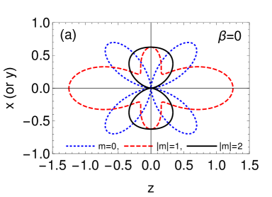
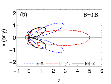
Figure 1: Angular distributions of the quadrupole radiation of $|m|=0,1$ and 2 in dotted blue, dashed red and solid black respectively. (a) $\beta=0$ and (b) $\beta=0.6$.

The emission process is classified by its multipole nature. Denoting the projection of angular momentum onto the quantization axis by $m$, a quadrupole or higher multipole radiation of $|m|\neq 1$ possesses an OAM and a beam of twisted photons is obtained if the parent ions are boosted. In particular, beams of $|m|\geq 2$ are nontrivial in the sense that one can access target states of larger magnetic quantum numbers with such beams. It is impossible to make a transition of $|\Delta m|\geq 2$ with a plane wave in single-photon absorption. In the numerical illustration in Sec. 3, we consider the deexcitation from the $3d_{5/2}$ state of hydrogen-like ions to the ground state, which is dominated by the electric quadrupole (E2) radiation. In Fig. 1, we illustrate the angular distributions of the quadrupole radiation in (a) the rest frame of the ion and (b) the laboratory frame in which the ion is accelerated as $\beta=0.6$. The distribution of $|m|=2$ vanishes on the $z$ axis, which indicates the phase singularity along the beam axis and exhibits the nature of twisted photons.

2.1 Bessel beam

The Bessel beam is an instance of light beams with OAM. In this work, we suppose that a Bessel beam is irradiated to excite an ion to a state that is able to emit a twisted photon in its deexcitation process.

A Bessel beam propagating along the $z$ axis is represented by the following superposition of plane waves [31, 32]:

$$A^{\mu}_{m_{\gamma}\kappa_{\gamma}\lambda}(t_{,}\bm{r}):=\int a_{m_{\gamma}\kappa_{\gamma}}(\bm{k}_{T})A^{\mu}_{\bm{k}\lambda}(t_{,}\bm{r})\frac{d^{2}k_{T}}{(2\pi)^{2}}\,,$$ (4)

where

$$a_{m_{\gamma}\kappa_{\gamma}}(\bm{k}_{T}):=(-i)^{m_{\gamma}}e^{im_{\gamma}\varphi_{k}}\sqrt{\frac{2\pi}{\kappa_{\gamma}}}\delta(|\bm{k}_{T}|-\kappa_{\gamma})$$ (5)

is the weight of the superposition for a given photon transverse wave vector $\bm{k}_{T}$. The plane-wave field of wave vector $\bm{k}$ and helicity $\lambda$ is given by

$$A^{\mu}_{\bm{k}\lambda}(t_{,}\bm{r}):=\frac{1}{\sqrt{2\omega}}\epsilon^{\mu}_{\lambda}(\bm{k})e^{-i(\omega t-\bm{k}\cdot\bm{r})}\,,\ \omega=|\bm{k}|\,,$$ (6)

where $\epsilon^{\mu}_{\lambda}(\bm{k})$ is the polarization vector. The wave vector of plane wave is parameterized as $\bm{k}=k(\sin\theta_{k}\cos\varphi_{k},\sin\theta_{k}\sin\varphi_{k},\cos\theta_{k})$, so that $\bm{k}\cdot\bm{x}=k_{z}z+\bm{k}_{T}\cdot\bm{x}_{T}$, $k_{z}=k\cos\theta_{k}$ and $\bm{k}_{T}=k\sin\theta_{k}(\cos\varphi_{k},\sin\varphi_{k},0)$. The polar angle $\theta_{k}$ is called the pitch angle. We note that $m_{\gamma}$ represents the eigenvalue of $J_{z}$, the $z$ component of the total angular momentum, and $\kappa_{\gamma}=|\bm{k}_{T}|=|\bm{k}|\sin\theta_{k}$.

When a Bessel beam is irradiated on an ion, the target ion is not always on the axis of the Bessel beam. We denote the impact parameter of the Bessel beam by $\bm{b}$ taking the position of the ionic nucleus as the origin of the coordinate system. Then, the electromagnetic field at the electronic position $\bm{r}$ is given by Eq. (4) with [42]

$$A^{\mu}_{\bm{k}\lambda}(t_{,}\bm{r}):=\frac{1}{\sqrt{2\omega}}\epsilon^{\mu}_{\lambda}(\bm{k})e^{-i(\omega t-\bm{k}\cdot\bm{r}-\bm{k}_{T}\cdot\bm{b})}\,.$$ (7)

2.2 Absorption of twisted photons by hydrogen-like heavy ions

In the following, we evaluate the absorption cross section in the rest frame of the ion. In this frame the resonant energy of the incident photon is $E_{eg}$, which is of order keV for heavy ions.

The interaction of the electron with the radiation field in the Dirac theory is given by

$$H_{I}=e\bm{\alpha}\cdot\bm{A}\,,$$ (8)

where $e=|e|$ is the unit charge and $\bm{\alpha}$ represents the Dirac matrices. The absorption amplitude is given by a matrix element of $V=H_{I}e^{i\omega t}$.

2.2.1 Amplitude superposition

It is convenient to express the twisted photon amplitude as a superposition of plane wave amplitudes like the twisted photon field itself. Then, the absorption amplitude is written as [43]

$$M_{fi}^{\text{(tw)}}=\langle f|V^{\text{(tw)}}|i\rangle=\int\frac{d^{2}k_{T}}{(2\pi)^{2}}a_{m_{\gamma}\kappa_{\gamma}}(\bm{k}_{T})e^{-i\bm{k}_{T}\cdot\bm{b}}M_{fi}^{\text{(pl)}}(\theta_{k},\varphi_{k})$$ (9)

where $M_{fi}^{\text{(pl)}}(\theta_{k},\varphi_{k}):=\langle f|V^{\text{(pl)}}|i\rangle$ is the plane wave amplitude in which the direction of the photon wave vector is specified by $\theta_{k}$ and $\varphi_{k}$ with respect to the ionic spin quantization axis (taken to be the $z$ axis). Such an inclined plane wave amplitude is expressed as

$$M_{fi}^{\text{(pl)}}(\theta_{k},\varphi_{k})=e^{-i(m_{f}-m_{i})\varphi_{k}}\sum_{m^{\prime}_{f}m^{\prime}_{i}}d_{m_{f}m^{\prime}_{f}}^{j_{f}}(\theta_{k})d_{m_{i}m^{\prime}_{i}}^{j_{i}}(\theta_{k})M_{m^{\prime}_{f}m^{\prime}_{i}}\,,$$ (10)

where $d_{mm^{\prime}}^{j}(\theta)$ is Wigner’s d-function and $M_{m^{\prime}_{f}m^{\prime}_{i}}$ represents the ordinary plane wave amplitude of $\theta_{k}=\varphi_{k}=0$. Substituting Eq. (10) into Eq. (9), one obtains

$$M_{fi}^{\text{(tw)}} =(-i)^{2m_{\gamma}+m_{i}-m_{f}}e^{i(m_{\gamma}+m_{i}-m_{f})\varphi_{b}}\sqrt{\frac{\kappa_{\gamma}}{2\pi}}J_{m_{\gamma}+m_{i}-m_{f}}(\kappa_{\gamma}b)M_{fi}^{\text{(pl)}}(\theta_{k},0)$$

$$=:\mathcal{M}_{m_{f}m_{i}}(\bm{b})\,,$$ (11)

where $\varphi_{b}$ denotes the azimuthal angle of $\bm{b}$.

2.2.2 Plane wave amplitude in the Dirac theory

Here, we consider hydrogen-like ions in the Dirac theory. (See e.g. Ref. [44].) The wave function is given by

$$\psi_{n\kappa m}(\bm{r})=\begin{pmatrix}\displaystyle{\frac{G_{n\kappa}(r)}{r}}\Omega_{jm}^{\ell_{A}}(\theta,\varphi)\\[8.61108pt] i\displaystyle{\frac{F_{n\kappa}(r)}{r}}\Omega_{jm}^{\ell_{B}}(\theta,\varphi)\end{pmatrix}\,,$$ (12)

where $\kappa=\mp(j+1/2)$, $\ell_{A}=j\mp 1/2$, $\ell_{B}=j\pm 1/2$ and $\Omega_{jm}^{\ell}(\theta,\varphi)$ denotes the spinor spherical harmonics. The wave function is normalized as $\int d^{3}r\,|\psi_{n\kappa m}(\bm{r})|^{2}=\int dr\,\{G_{n\kappa}^{2}(r)+F_{n\kappa}^{2}(r)\}=1$. The electronic state of an ion may be denoted as $|n,\kappa,m\rangle$.

The plane wave matrix element in the right-hand side of Eq. (10) is expressed as

$$M_{m_{f}m_{i}}=\langle n_{f},\kappa_{f},m_{f}|V^{\text{(pl)}}|n_{i},\kappa_{i},m_{i}\rangle\,.$$ (13)

Using the Dirac wave function in Eq. (12) and the plane wave field in Eq. (6), we find that

$$M_{m_{f}m_{i}}= -ie\sqrt{\frac{3}{\omega}}(-1)^{j_{i}+m_{f}}\sqrt{(2j_{f}+1)(2j_{i}+1)}\,\delta_{m_{f},m_{i}+\lambda}$$

$$\times\sum_{j,\ell}(-1)^{j}i^{\ell}\sqrt{2\ell+1}\,C_{j_{f}-m_{f},j_{i}m_{i}}^{j-m_{f}+m_{i}}C_{\ell-m_{f}+m_{i}+\lambda,1-\lambda}^{j-m_{f}+m_{i}}$$

$$\phantom{\times\sum}\left[(-1)^{\ell_{Af}}\sqrt{(2\ell_{Af}+1)(2\ell_{Bi}+1)}\,C_{\ell_{Af}0,\ell_{Bi}0}^{\ell 0}\begin{Bmatrix}\ell_{Af}&j_{f}&1/2\\ \ell_{Bi}&j_{i}&1/2\\ \ell&j&1\end{Bmatrix}\mathcal{I}_{GF}^{\ell}\right.$$

$$\phantom{\times\sum}\left.-(-1)^{\ell_{Bf}}\sqrt{(2\ell_{Bf}+1)(2\ell_{Ai}+1)}\,C_{\ell_{Bf}0,\ell_{Ai}0}^{\ell 0}\begin{Bmatrix}\ell_{Bf}&j_{f}&1/2\\ \ell_{Ai}&j_{i}&1/2\\ \ell&j&1\end{Bmatrix}\mathcal{I}_{FG}^{\ell}\right]\,,$$ (14)

where $C_{j_{1}m_{1},j_{2}m_{2}}^{j_{3}m_{3}}$ is the Clebsch-Gordan coefficient and

$$\begin{Bmatrix}a&b&c\\ d&e&f\\ g&h&i\end{Bmatrix}$$ (15)

represents the $9j$ symbol, e.g. [45]. The radial integrals are defined by

$$\mathcal{I}_{GF}^{\ell}:=\int dr\,j_{\ell}(kr)G_{f}(r)F_{i}(r)\,,\ \mathcal{I}_{FG}^{\ell}:=\int dr\,j_{\ell}(kr)F_{f}(r)G_{i}(r)\,,$$ (16)

where $j_{\ell}(kr)$ denotes the spherical Bessel function and $k=|\bm{k}|$ is the wave number of the plane wave photon.

2.2.3 Absorption cross section

The absorption rate of a twisted photon is proportional to the squared amplitude in Eq. (11)

$$|\mathcal{M}_{m_{f}m_{i}}(\bm{b})|^{2}=(\kappa_{\gamma}/2\pi)|M^{\text{(pl)}}_{m_{f}m_{i}}(\theta_{k},0)|^{2}J^{2}_{m_{\gamma}+m_{i}-m_{f}}(\kappa_{\gamma}b)\,.$$ (17)

In experiments where the ion beam is not sufficiently collimated (as virtually all experiments we envisage), it is legitimate to average over the impact parameter $\bm{b}$. Provided that the (effective) beam radius $R$ is large enough as $\kappa_{\gamma}R\gg 1$, (fat beam approximation), one obtains

$$\frac{1}{\pi R^{2}}\int|\mathcal{M}_{m_{f}m_{i}}(\bm{b})|^{2}d^{2}b\simeq\frac{1}{\pi^{2}R}|M^{\text{(pl)}}_{m_{f}m_{i}}(\theta_{k},0)|^{2}\,,$$ (18)

where we have used the asymptotic form of the Bessel function, $J_{m}(z)\simeq\sqrt{2/\pi z}\,\cos(z-\pi/4-m\pi/2)$. We note that the $m_{\gamma}$ dependence disappears in this approximation.

The photon number flux of the Bessel beam is given by $f(R)=\cos\theta_{k}/\pi^{2}R$ in the fat beam approximation [32]. With this flux, we obtain the absorption cross section for a given set of initial and final magnetic quantum numbers as

$$\sigma(\omega)=\frac{2}{\cos\theta_{k}}\frac{\Gamma_{f}/2}{(\omega+E_{i}-E_{f})^{2}+\Gamma_{f}^{2}/4}|M^{\text{(pl)}}_{m_{f}m_{i}}(\theta_{k},0)|^{2}\,,$$ (19)

where $E_{i(f)}$ is the energy of the initial (final) state and $\Gamma_{f}$ denotes the natural width of the final state.

2.3 Emission of twisted photons by hydrogen-like heavy ions

The photons emitted in multipole radiations of $j\geq 2$ are twisted in the sense that they have nonzero orbital angular momentum. Accordingly, we consider the multipole radiations of hydrogen-like heavy ions.

The interaction hamiltonian $H_{I}=-e\gamma_{\mu}A^{\mu}$ in which the electromagnetic field is one of the multipole fields introduced below describes the multipole emission. The emission rate of $|i\rangle\to|f\rangle+\gamma$ is given by

$$dw=2\pi|V_{fi}|^{2}\delta(E_{i}-E_{f}-\omega)d\omega\,,\ w=2\pi|V_{fi}|^{2}\,,$$ (20)

where $V_{fi}=\langle f|H_{I}e^{-i\omega t}|i\rangle$ is the emission matrix element. We work in the rest frame of the ion as in the evaluation of the absorption cross section.

We do not employ the long wavelength approximation. The scale of transition wavelengths is $1/(Z\alpha)^{2}m_{e}$, and the size of an ion is $\sim 1/Z\alpha m_{e}$. In the case $Z\alpha\ll 1$, the long wavelength approximation is legitimate. For heavy ions of $Z\alpha=O(1)$, the long wavelength approximation is questionable.

2.3.1 Multipole fields

In the Coulomb gauge, the multipole vector potentials are written in terms of the vector spherical harmonics, $\bm{Y}_{jm}^{\ell}(\bm{n})$. We note that

$$\hat{\bm{J}}^{2}\bm{Y}_{jm}^{\ell}=j(j+1)\bm{Y}_{jm}^{\ell}\,,\ \hat{J}_{z}\bm{Y}_{jm}^{\ell}=m\bm{Y}_{jm}^{\ell}\,,$$ (21)

$$\hat{\bm{L}}^{2}\bm{Y}_{jm}^{\ell}=\ell(\ell+1)\bm{Y}_{jm}^{\ell}\,,\ \hat{\bm{S}}^{2}\bm{Y}_{jm}^{\ell}=2\bm{Y}_{jm}^{\ell}\,.$$ (22)

The vector spherical harmonics may be expressed as $\bm{Y}_{jm}^{\ell}(\bm{n})=\sum_{m,\sigma}C^{jm}_{\ell m,1\sigma}Y_{\ell m}(\bm{n})\bm{e}_{\sigma}$, where $\bm{e}_{\sigma}$ denotes the covariant spherical basis vectors, $\bm{e}_{\pm 1}=\mp(\bm{e}_{x}\pm i\bm{e}_{y})/\sqrt{2}$ and $\bm{e}_{0}=\bm{e}_{z}$ [45].

The electric multipole field of angular frequency $\omega$ and wave vector $\bm{k}$ is given by

$$\bm{A}_{\omega jm}(\bm{k})=2(\pi/\omega)^{3/2}\delta(|\bm{k}|-\omega)\bm{Y}^{(e)}_{jm}(\hat{\bm{k}})\,,$$ (23)

where

$$\bm{Y}^{(e)}_{jm}(\hat{\bm{k}}):=\frac{1}{\sqrt{j(j+1)}}\bm{\nabla}_{\hat{\bm{k}}}Y_{jm}(\hat{\bm{k}})=\sqrt{\frac{j+1}{2j+1}}\bm{Y}_{jm}^{j-1}+\sqrt{\frac{j}{2j+1}}\bm{Y}_{jm}^{j+1}\,.$$ (24)

The magnetic multipole field is written as

$$\bm{A}_{\omega jm}(\bm{k})=2(\pi/\omega)^{3/2}\delta(|\bm{k}|-\omega)\bm{Y}^{(m)}_{jm}(\hat{\bm{k}})\,,$$ (25)

where

$$\bm{Y}^{(m)}_{jm}(\hat{\bm{k}}):=\hat{\bm{k}}\times\bm{Y}^{(e)}_{jm}(\hat{\bm{k}})=i\bm{Y}_{jm}^{j}\,.$$ (26)

We note that

$$\int d\Omega_{\hat{\bm{k}}}\bm{Y}^{(e)*}_{jm}(\hat{\bm{k}})\cdot\bm{Y}^{(e)}_{j^{\prime}m^{\prime}}(\hat{\bm{k}})=\int d\Omega_{\hat{\bm{k}}}\bm{Y}^{(m)*}_{jm}(\hat{\bm{k}})\cdot\bm{Y}^{(m)}_{j^{\prime}m^{\prime}}(\hat{\bm{k}})=\delta_{jj^{\prime}}\delta_{mm^{\prime}}\,.$$ (27)

The parities of the electric and magnetic multipole fields are opposite. We assign $(-1)^{j}$ to the electric multipole field in Eq. (23) and $(-1)^{j+1}$ to the magnetic multipole field in Eq. (25). For instance, the electric (magnetic) dipole field is parity odd (even).

In the coordinate space, the field is given by

$$\bm{A}_{\omega jm}(\bm{r})=\int\frac{dk^{3}}{(2\pi)^{3}}\bm{A}_{\omega jm}(\bm{k})e^{i\bm{k}\cdot\bm{r}}\,.$$ (28)

2.3.2 Electric multipole radiations in the Dirac theory

Since the electric multipole field contains two components of orbital angular momentum, $\ell=j\pm 1$, as seen in Eq. (24), we rearrange them by a gauge transformation [46]. A gauge transformation results in the following vector and scalar potentials:

$$\bm{A}_{\omega jm}(\bm{k})=2(\pi/\omega)^{3/2}\delta(|\bm{k}|-\omega)\left\{\bm{Y}^{(e)}_{jm}(\hat{\bm{k}})+C\hat{\bm{k}}Y_{jm}(\hat{\bm{k}})\right\}\,,$$ (29)

$$\phi_{\omega jm}(\bm{k})=2(\pi/\omega)^{3/2}\delta(|\bm{k}|-\omega)CY_{jm}(\hat{\bm{k}})\,,$$ (30)

where $C$ is a gauge parameter. Choosing $C=-\sqrt{(j+1)/j}$, we obtain

$$\bm{A}_{\omega jm}^{(e)}(\bm{k})=\sqrt{(2j+1)/j}\,2(\pi/\omega)^{3/2}\delta(|\bm{k}|-\omega)\bm{Y}_{jm}^{j+1}(\hat{\bm{k}})\,,$$ (31)

$$\phi_{\omega jm}^{(e)}(\bm{k})=-\sqrt{(j+1)/j}\,2(\pi/\omega)^{3/2}\delta(|\bm{k}|-\omega)Y_{jm}(\hat{\bm{k}})\,.$$ (32)

In the long wavelength approximation, $\phi_{\omega jm}^{(e)}$ dominantly contributes and $\bm{A}_{\omega jm}^{(e)}(\bm{k})$ does subdominantly. As we mentioned above, we consider both contributions for heavy ions.

The contribution of the scalar potential in Eq. (32) to the emission matrix element is given by

$$V_{fi}^{(\phi)} =-e\int d^{3}r\psi_{f}^{\dagger}(\bm{r})\psi_{i}(\bm{r})\int\frac{d^{3}k}{(2\pi)^{3}}\phi_{\omega jm}^{(e)*}(\bm{k})e^{-i\bm{k}\cdot\bm{r}}$$ (33)

$$=e\sqrt{\frac{j+1}{j}}\frac{\sqrt{\omega}}{4\pi^{3/2}}\int d^{3}r\psi_{f}^{\dagger}(\bm{r})\psi_{i}(\bm{r})\int d\Omega_{k}e^{-i\bm{k}\cdot\bm{r}}Y_{jm}^{*}(\hat{\bm{k}})\,,$$ (34)

where $\psi_{i(f)}(\bm{r})$ represents the initial (final) wave function given in Eq. (12). The angular integral over $\Omega_{k}$ is performed using

$$e^{i\bm{k}\cdot\bm{r}}=4\pi\sum_{\ell=0}^{\infty}\sum_{m=-\ell}^{m=\ell}i^{\ell}j_{\ell}(kr)Y^{*}_{\ell m}(\hat{\bm{k}})Y_{\ell m}(\hat{\bm{r}})\,,$$ (35)

and one obtains

$$V_{fi}^{(\phi)}=e(-i)^{j}\sqrt{\frac{j+1}{j}}\sqrt{\frac{\omega}{\pi}}\int d^{3}r\psi_{f}^{\dagger}(\bm{r})\psi_{i}(\bm{r})j_{j}(kr)Y_{jm}^{*}(\hat{\bm{r}})\,.$$ (36)

Substituting the Dirac wave function in Eq. (12) and integrating over the remaining angular variables, we obtain

$$V_{fi}^{(\phi)}= \frac{e}{2\pi}\sqrt{\omega}\,i^{j}(-1)^{j_{f}+m_{f}+j_{i}+1/2}\,\sqrt{\frac{(j+1)(2j_{f}+1)(2j_{i}+1)}{j(2j+1)}}\,C^{j-m_{f}+m_{i}}_{j_{f}-m_{f},j_{i}m_{i}}$$

$$\times\left[\begin{Bmatrix}\ell_{Af}&\ell_{Ai}&j\\ j_{i}&j_{f}&1/2\end{Bmatrix}\sqrt{(2\ell_{Af}+1)(2\ell_{Ai}+1)}\,C^{j0}_{\ell_{Af}0,\ell_{Ai}0}\,\mathcal{I}^{j}_{GG}\right.$$

$$\quad\left.+\begin{Bmatrix}\ell_{Bf}&\ell_{Bi}&j\\ j_{i}&j_{f}&1/2\end{Bmatrix}\sqrt{(2\ell_{Bf}+1)(2\ell_{Bi}+1)}\,C^{j0}_{\ell_{Bf}0,\ell_{Bi}0}\,\mathcal{I}^{j}_{FF}\right]\,,$$ (37)

where

$$\begin{Bmatrix}a&b&c\\ d&e&f\end{Bmatrix}$$ (38)

represents the $6j$ symbol and the radial integrals are given by

$$\mathcal{I}_{GG}^{j}:=\int dr\,j_{\ell}(kr)G_{f}(r)G_{i}(r)\,,\ \mathcal{I}_{FF}^{j}:=\int dr\,j_{\ell}(kr)F_{f}(r)F_{i}(r)\,.$$ (39)

As for the contribution of the vector potential in Eq. (31), the $\bm{k}$ integration results in

$$V_{fi}^{(A)}=e(-i)^{j+1}\sqrt{\frac{2j+1}{j}}\sqrt{\frac{\omega}{\pi}}\int d^{3}rj_{j+1}(kr)\psi_{f}^{\dagger}(\bm{r})\bm{\alpha}\psi_{i}(\bm{r})\cdot\bm{Y}_{jm}^{j+1*}(\hat{\bm{r}})\,.$$ (40)

Integrating over $\bm{r}$, we find

$$V_{fi}^{(A)}= \frac{e}{2\pi}\sqrt{\omega}\,i^{j}(-1)^{j_{i}+m_{f}}\,\sqrt{\frac{6(2j+1)(2j_{f}+1)(2j_{i}+1)}{j}}\,C^{j-m_{f}+m_{i}}_{j_{f}-m_{f},j_{i}m_{i}}$$

$$\times\left[\begin{Bmatrix}\ell_{Af}&j_{f}&1/2\\ \ell_{Bi}&j_{i}&1/2\\ j+1&j&1\end{Bmatrix}(-1)^{\ell_{Af}}\sqrt{(2\ell_{Af}+1)(2\ell_{Bi}+1)}\,C^{j+10}_{\ell_{Af}0,\ell_{Bi}0}\,\mathcal{I}^{j+1}_{GF}\right.$$

$$\quad\left.-\begin{Bmatrix}\ell_{Bf}&j_{f}&1/2\\ \ell_{Ai}&j_{i}&1/2\\ j+1&j&1\end{Bmatrix}(-1)^{\ell_{Bf}}\sqrt{(2\ell_{Bf}+1)(2\ell_{Ai}+1)}\,C^{j+10}_{\ell_{Bf}0,\ell_{Ai}0}\,\mathcal{I}^{j+1}_{FG}\right]\,.$$ (41)

The total amplitude is $V_{fi}=V_{fi}^{(\phi)}+V_{fi}^{(A)}$.

2.3.3 Magnetic multipole radiations in the Dirac theory

The magnetic multipole radiation is described by the vector potential in Eq. (25). The emission matrix element is evaluated in the similar manner as $V_{fi}^{(A)}$ above and we obtain

$$V_{fi}= \frac{e}{2\pi}\sqrt{\omega}\,i^{j}(-1)^{j_{i}+m_{f}}\,\sqrt{6(2j_{f}+1)(2j_{i}+1)}\,C^{j-m_{f}+m_{i}}_{j_{f}-m_{f},j_{i}m_{i}}$$

$$\times\left[\begin{Bmatrix}\ell_{Af}&j_{f}&1/2\\ \ell_{Bi}&j_{i}&1/2\\ j&j&1\end{Bmatrix}(-1)^{\ell_{Af}}\sqrt{(2\ell_{Af}+1)(2\ell_{Bi}+1)}\,C^{j0}_{\ell_{Af}0,\ell_{Bi}0}\,\mathcal{I}^{j}_{GF}\right.$$

$$\quad\left.-\begin{Bmatrix}\ell_{Bf}&j_{f}&1/2\\ \ell_{Ai}&j_{i}&1/2\\ j&j&1\end{Bmatrix}(-1)^{\ell_{Bf}}\sqrt{(2\ell_{Bf}+1)(2\ell_{Ai}+1)}\,C^{j0}_{\ell_{Bf}0,\ell_{Ai}0}\,\mathcal{I}^{j}_{FG}\right]\,.$$ (42)

3 Numerical results

As an illustration, we consider the excitation of H-like ions from the ground state $1\text{s}_{1/2}$ to the excited state of $3\text{d}_{5/2}$ by the Bessel beam and the successive deexcitation back to the ground state by the E2 emission. If the magnetic quantum number of the ground state differs from that of the exited state by two (or larger), this process is not possible with the plane-wave beam nor the dipole emission.

For instance, one may consider $2\text{p}_{3/2}$ instead of $3\text{d}_{5/2}$. The excitation to the state of $|m|=3/2$ is possible with the plane-wave beam. This is an E1 transition and its rate is significant. However, the subsequent deexcitation from $2\text{p}_{3/2}(m=\pm 3/2)$ to $1\text{s}_{1/2}(m=\mp 1/2)$, which generates a twisted gamma ray of $|m|=2$, is the magnetic quadrupole (M2) transition. It turns out that, even for Pb, this M2 rate is suppressed by a factor of $\sim 10^{3}$ compared to the dominant E1 emission of an untwisted photon. This E1 photon becomes a serious background because its energy is the same as the M2 photon.

3.1 Excitation rate with twisted photons

The resonant excitation rate is described by the absorption cross section in Eq. (19) with $\omega=E_{eg}=E(3\text{d}_{5/2})-E(1\text{s}_{1/2})$ and presented in Fig. 2 as a function of the pitch angle $\theta_{k}$. We choose $m_{i}=1/2$, $m_{f}=5/2$ and $\lambda=1$.

The target ion is H-like Pb ($Z=82$) in Fig. 2(a). The level splitting is $E_{eg}=91.3$ keV. The energy of the excitation laser is taken as $\omega_{i}=10$ eV, and this implies $\gamma=4.57\times 10^{3}$ and $\omega_{f}^{\text{max}}=0.834$ GeV. The width of the excited state is dominated by the major E1 rate, $\Gamma_{f}\simeq\Gamma(3\text{d}_{5/2}\to 2\text{p}_{3/2})=1.89$ eV.

In Fig. 2(b), the ion is H-like Ne ($Z=10$) and we take $\omega_{i}=1$ eV. The relevant parameters in this case are $\gamma=606$, $\omega_{f}^{\text{max}}=1.47$ MeV and $\Gamma_{f}\simeq 4.26\times 10^{-4}$ eV. The much larger cross section of Ne than Pb is due to the narrow width of the $3\text{d}_{5/2}$ state.

 

Figure 2: Absorption cross section of $1\text{s}_{1/2,\,m=1/2}\to 3\text{d}_{5/2,\,m=5/2}$. The photon helicity is $\lambda=1$. (a) The target ion is Pb with $\omega_{i}=10$ eV. (b) Ne with $\omega_{i}=1$ eV. We note the difference in the units of the vertical axes.

The pitch angle $\theta_{k}$ can be $O(1)$ in the laboratory frame. While, in the rest frame of the ion, it is $O(1/\gamma)$ because the transverse momentum $\bm{k}_{T}$ of twisted photons is invariant under the Lorentz boost. We have chosen the ranges of the horizontal axis in Fig. 2 following this observation and the difference of $\omega_{i}$’s for the two species of ion. The absorption cross section is proportional to $\theta_{k}^{2}$ for $|\theta_{k}|\ll 1$ as seen in Fig. 2. The case of $\theta_{k}=0$ corresponds to a plane wave, and the cross section vanishes since the process of $|m_{f}-m_{i}|>1$ is impossible with the plane wave as mentioned above.

3.2 Emission rate of twisted photons

The E2 transition rate from $3\text{d}_{5/2}$ to $1\text{s}_{1/2}$ is given by Eqs. (20), (37) and (41) with $j=2$. In Fig. 3(a), we present the E2 transition rate of H-like ion as a function of $Z$. The dominant E1 rate from $3\text{d}_{5/2}$ to $2\text{p}_{3/2}$ is also shown for comparison. The ratio of the E2 rate to the E1 rate, which gives an approximate branching fraction to emit an E2 photon, is given in Fig. 3(b). We observe that the E2 rate depends on $Z$ as $Z^{6}$ in good precision, while the E1 is approximately proportional to $Z^{4}$, so that heavier ions exhibit larger branching fractions of emitting a twisted photon.

 

Figure 3: (a) E2 rate compared to E1. (b) Ratio of E2 to E1.

For H-like Pb, we find $\Gamma(3\text{d}_{5/2}\to 1\text{s}_{1/2})=8.49\times 10^{-2}$ eV, so that the branching fraction of the E2 transition is $\text{Br}(3\text{d}_{5/2}\to 1\text{s}_{1/2})\simeq 4.5\times 10^{-2}$. As for H-like Ne, $\Gamma(3\text{d}_{5/2}\to 1\text{s}_{1/2})=3.89\times 10^{-7}$ eV, and $\text{Br}(3\text{d}_{5/2}\to 1\text{s}_{1/2})\simeq 9.1\times 10^{-4}$.

3.3 Characteristics of photons generated by the method

In the excitation process in Sec. 3.1, the final state of $m_{f}=3/2$, in addition to $m_{f}=5/2$, is also possible with the same Bessel beam. Then, the $3\text{d}_{5/2}(m=3/2)$ state deexcites to the ground state ($1\text{s}_{1/2}$) by the E2 emission of $m=1$. Its emission pattern is shown in Fig. 1(b) (the red dashed line) and exhibits no phase singularity on the $z$ axis. So that, the photon in this process is not twisted and could be a source of backgrounds.

It turns out that the $m_{f}=3/2$ process dominates the absorption cross section as $\sigma_{m_{f}=5/2}/\sigma_{m_{f}=3/2}\simeq 6\times 10^{-8}(3\times 10^{-6})$ for H-like Pb (Ne) in the case of $\theta=1/\gamma$. This is because the process of $|m_{f}-m_{i}|=1$ is possible with the plane wave and the cross section does not vanish even if $\theta_{k}=0$. We note that the above ratios are $O(\theta_{k}^{2})=O(1/\gamma^{2})$.

4 Summary

We first point out two important aspects of the method we proposed in this article: one is its final flux of gamma rays with OAM and the other is associated backgrounds. As shown in Fig. 2, the absorption cross sections are in a range of a few tens of mb (for $Z=82$) to b (for $Z=10$). The achievable flux depends heavily upon actual experimental configurations, in particular accelerators and incident lasers. Considering current technologies, we expect reasonable flux useful to a variety of physics.

As to the backgrounds, we expect two major backgrounds in this method as discussed in the previous section: one is due to the process from d-states to p-states and the other from $m_{f}=3/2$ of the d-states to s-states. The former type of the backgrounds has a different energy from that of the signal, i.e. the gamma rays with OAM. Whether they are tolerable or not depends upon details of particular experiments, for example detectors employed or reactions in interests may or may not be sensitive to such backgrounds. In general, however, it is desirable to reduce them; from this view point, we believe it important to consider other ion types than the hydrogen-like ions. On the other hand, the second type of the backgrounds has the same energy with the signal. In this case, it is highly recommended to eliminate or reduce these backgrounds. One way to eliminate such backgrounds is to introduce a transverse magnetic field $\bm{B}_{T}$ in the production region. The Zeeman effect splits each magnetic quantum number $m_{f}$, one of which (i.e. $m_{f}=5/2$) can be selected by choosing the frequency of the excitation photons. Note that $\bm{B}_{T}$ is amplified by the Lorentz boost factor $\gamma$ when seen by the ions. Also note that it is necessary to rotate the spin from transverse to longitudinal. Designing actual spin rotation systems requires more detailed studies, which is underway currently.

In summary, we have studied an alternative method of generating gamma rays with OAM. It exploits accelerated partially-stripped ions as an energy upconverter. Relativistic calculations are performed to calculate the excitation cross section and deexcitation rate for hydrogen-like ions, and their properties including flux and possible backgrounds are discussed.

References

- [1] J.H. Poynting, “The wave motion of a revolving shaft, and a suggestion as to the angular momentum in a beam of circularly polarised light”, Proc. RṠoc. London, Ser. A 82, 560567 (1909).
- [2] R.A. Beth, “Mechanical detection and measurement of the angular momentum of light”, Phys. Rev. 50, 115 (1936).
- [3] L. Allen, et al. “Orbital angular momentum of light and the transformation of Laguerre-Gaussian laser modes.” Phys. Rev. A 45, 8185 (1992).
- [4] Y. Shen et al. “Optical vortices 30 years on: OAM manipulation from topological charge to multiple singularities”, Light: Science & Applications 8:90 (2019). https://doi.org/10.1038/s41377-019-0194-2
- [5] M.J. Padgett, “Orbital angular momentum 25 years on”, Opt. Express 25, 11265 (2017).
- [6] G. Molina-Terriza, J.P. Torres and L. Torner, “Twisted photons”, Nat. Phys. 3, 305 (2007).
- [7] J.P. Torres and L. Torner (eds.), “Twisted photons”, Wiley-VCH Weinheim, Germany, 2011.
- [8] M. Babiker, D.L. Andrews and V.E. Lembessis, “Atoms in complex twisted light”, J. Opt. 21, 013001 (2019).
- [9] M. Solyanik-Gorgone, A. Afanasev, C.E. Carlson, C.T. Schmiegelow and F. Schmidt-Kaler, “Excitation of E1-forbidden atomic transitions with electric, magnetic, or mixed multipolarity in light fields carrying orbital and spin angular momentum”, J. Opt. Soc. Am. B 36, 565 (2019).
- [10] A. Mair, A. Vaziri, G. Weihs and A. Zeilinger, “Entanglement of the orbital angular momentum states of photons”, Nature 412, 313 (2001).
- [11] J. Leach, B. Jack, J. Romero, M. Ritsch-Marte, R.W. Boyd, A.K. Jha, S.M. Barnett, S. Franke-Arnold and M.J. Padgett, “Violation of a Bell inequality in two-dimensional orbital angular momentum state-spaces”, Opt. Express 17, 8287 (2009).
- [12] H. He, M.E.J. Friese, N.R. Heckenberg and H. Rubinsztein-Dunlop, “Direct observation of transfer of angular momentum to absorptive particles from a laser beam with a phase singularity”, Phys. Rev. Lett. 75, 826 (1995).
- [13] V. Garcés-Chávez, D. McGloin, M.J. Padgett, W. Dultz, H. Schmitzer and K. Dholakia, “Observation of the transfer of the local angular momentum density of a multiringed light beam to an optically trapped particle”, Phys. Rev. Lett. 91, 093602 (2003).
- [14] G.A. Swartzlander, “Peering into darkness with a vortex spatial filter”, Opt. Lett. 26, 497 (2001).
- [15] G.A. Swartzlander Jr., E.L. Ford, R.S. Abdul-Malik, L.M. Close, M.A. Peters, D.M. Palacios and D.W. Wilson, “Astronomical demonstration of an optical vortex coronagraph”, Opt. Express 16, 10200 (2008).
- [16] S. Fürhapter, A. Jesacher, S. Bernet and M. Ritsch-Marte, “Spiral interferometry”, Opt. Lett. 30, 1953 (2005).
- [17] M. Erhard, R. Fickler, M. Krenn and A. Zeilinger, “Twisted photons: new quantum perspectives in high dimensions”, Light: Science & Applications 7, 17146 (2018).
- [18] G. Gibson, J. Courtial, M.J. Padgett, M. Vasnetsov, V. Pas’ko, S.M. Barnett and S, Franke-Arnold, “Free-space information transfer using light beams carrying orbital angular momentum”, Opt. Express 12, 5448 (2004).
- [19] M. Krenn, J. Handsteiner, M. Fink, R. Fickler, R. Ursin, M. Malik and A. Zeilinger, “Twisted light transmission over 143 km”, Proc. Natl. Acad. Sci. U.S.A. 113, 13648 (2016).
- [20] M. Harwit, “Photon orbital angular momentum in astrophysics”, Astrophys. J. 597, 1266 (2003).
- [21] F. Tamburini, B. Thide and M.D. Valle, “Measurement of the spin of the M87 black hole from its observed twisted light”, MNRAS 492, L22 (2020).
- [22] Xuewen Wang, Zhongquan Nie, Yao Liang, Jian Wang, Tao Li and Baohua Jia, “Recent advances on optical vortex generation”, Nanophotonics 7, 1533 (2018).
- [23] M.W. Beijersbergen, L. Allen, H.E.L.O. van der Veen and J.P. Woerdman, “Astigmatic laser mode converters and transfer of orbital angular momentum”, Optics Communications 96, 123 (1993).
- [24] L. Marrucci, C. Manzo and D. Paparo, “Optical spin-to-orbital angular momentum conversion in inhomogeneous anisotropic media”, Phys. Rev. Lett. 96, 163905 (2006).
- [25] S. Sasaki and I. McNulty, “Proposal for generating brilliant x-ray beams carrying orbital angular momentum”, Phys. Rev. Lett. 100, 124801 (2008).
- [26] J. Bahrdt, K. Holldack, P. Kuske, R. Müller, M. Scheer and P. Schmid, “First Observation of Photons Carrying Orbital Angular Momentum in Undulator Radiation”, Phys. Rev. Lett. 111, 034801 (2013).
- [27] T. Kaneyasu, Y. Hikosaka, M. Fujimoto, H. Iwayama, M. Hosaka, E. Shigemasa, M. Katoh, “Observation of an optical vortex beam from a helical undulator in the XUV region”, J. Synchrotron Rad. 24, 934, (2017).
- [28] E. Hemsing, A. Knyazik, F. O’Shea, A. Marinelli, P. Musumeci, O. Williams, S. Tochitsky and J.B. Rosenzweig, “Experimental observation of helical microbunching of a relativistic electron beam”, Appl. Phys. Lett. 100, 091110 (2012).
- [29] E. Hemsing, A. Knyazik, M. Dunning, D. Xiang, A. Marinelli, C. Hast and J.B. Rosenzweig, “Coherent optical vortices from relativistic electron beams”, Nat. Phys. 9, 549 (2013).
- [30] P.R. Ribic, B. Rösner, D. Gauthier, E. Allaria, F. Döring, L. Foglia, L. Giannessi, N. Mahne, M. Manfredda, C. Masciovecchio et al., “Extreme-ultraviolet vortices from a free-electron laser”, Phys. Rev. X 7, 031036 (2017).
- [31] U.D. Jentschura and V.G. Serbo, “Generation of high-energy photons with large orbital angular momentum by compton backscattering”, Phys. Rev. Lett. 106, 013001 (2011).
- [32] U.D. Jentschura and V.G. Serbo, Compton upconversion of twisted photons: Backscattering of particles with non-planar wave functions”, Eur. Phys. J. C 71, 1571 (2011).
- [33] I. Ivanov and V. Serbo, “Scattering of twisted particles: Extension to wave packets and orbital helicity”, Phys. Rev. A 84, 033804 (2011).
- [34] S. Stock, A. Surzhykov, S. Fritzsche and D. Seipt, “Compton scattering of twisted light: Angular distribution and polarization of scattered photons”, Phys. Rev. A 92, 013401 (2015).
- [35] V. Petrillo, G. Dattoli, I. Drebot and F. Nguyen, “Compton scattered X-gamma rays with orbital momentum”, Phys. Rev. Lett. 117, 123903 (2016).
- [36] Y. Taira, T. Hayakawa and M. Katoh, “Gamma-ray vortices from nonlinear inverse Thomson scattering of circularly polarized light”, Sci. Rep. 7, 5018 (2017).
- [37] Yue-Yue Chen, Karen Z. Hatsagortsyan, and Christoph H. Keitel, “Generation of twisted -ray radiation by nonlinear Thomson scattering of twisted light”, Matter Radiat. Extremes 4, 024401 (2019).
- [38] I.P. Ivanov, “Colliding particles carrying nonzero orbital angular momentum”, Phys. Rev. D 83, 093001 (2011).
- [39] D. Budker et al., “Atomic Physics Studies at the Gamma Factory at CERN”, Ann. Phys. (Berlin) 532, 2000204 (2020).
- [40] E.G. Bessonov, “Light sources based on relativistic ion beam”, Nucl. Instr. Meth. B 309, 92 (2013).
- [41] M.W. Krasny, “Gamma Factory, Proof-of-Principle Experiment”, CERN-SPSC-2019-031; SPSC-I-253.
- [42] O. Matula, A.G. Hayrapetyan, V.G Serbo, A. Surzhykov and S. Fritzsche, “Atomic ionization of hydrogen-like ions by twisted photons: angular distribution of emitted electrons”, J. Phys. B: At. Mol. Opt. Phys. 46, 205002, 2013.
- [43] H.M. Scholz-Marggraf, S. Fritzsche, V.G. Serbo, A. Afanasev and A. Surzhykov, “Absorption of twisted light by hydrogenlike atoms”, Phys. Rev. A 90, 013425, 2014.
- [44] J. Sakurai, Advanced Quantum Mechanics. Addison-Wesley, Reading, Massachusetts, 1967.
- [45] D.A. Varshalovich, A.N. Moskalev and V.K. Khersonskii, “Quantum Theory of Angular Momentum”, World Scientific, Singapore, 1988.
- [46] V.B. Berestetskii, E.M. Lifshitz and L.P. Pitaevskii, “Quantum Electrodynamics”, 2nd Edition, 1980, Pergamon Press, Oxford.