Hypoelliptic Entropy dissipation for stochastic differential equations

Abstract.

We study the convergence analysis for general degenerate and non-reversible stochastic differential equations (SDEs). We apply the Lyapunov method to analyze the Fokker-Planck equation, in which the Lyapunov functional is chosen as a weighted relative Fisher information functional. We derive a structure condition and formulate the Lyapunov constant explicitly. We prove the exponential convergence result for the probability density function towards its invariant distribution in the $L_{1}$ distance. Two examples are presented: underdamped Langevin dynamics with variable diffusion matrices and three oscillator chain models with nearest-neighbor couplings.

1. Introduction

Consider an Itô stochastic differential equation (SDE)

$$dX_{t}=b(X_{t})dt+\sqrt{2}a(X_{t})dB_{t},$$ (1)

where $X_{t}\in\mathbb{R}^{n+m}$ is a stochastic process with dimensions $m$, $n\in\mathbb{Z}_{+}$, $b\in{C^{\infty}(\mathbb{R}^{n+m};\mathbb{R}^{n+m})}$ is a smooth drift vector field, $a\in{C^{\infty}(\mathbb{R}^{n+m};\mathbb{R}^{(n+m)\times n})}$ is a smooth diffusion matrix, and $B_{t}$ is a standard Brownian motion in $\mathbb{R}^{n}$.

We study the long-time dynamical behaviors of SDE (1). How fast does the probability density function of SDE (1) converge to its invariant distribution? The convergence behavior of SDE (1) plays an essential role in both theory and applications. Theoretically, it is a core problem in probability [7, 25], non-equilibrium dynamics [16, 26, 29, 40, 48], differential geometry [10, 11] and ergodic theory [8, 32, 36, 43]. In applications, the convergence rate is useful for studying long-time molecular dynamics behaviors [17, 33, 45]. Nowadays, the convergence rate is important in estimating the speed of Markov-Chain-Monte-Carlo methods (MCMC). This is an emerging issue in artificial intelligence (AI), and Bayesian sampling algorithms [15, 17, 19, 45].

In the current framework, when the diffusion matrix $a$ is non-degenerate, and the drift vector field $b$ is a gradient vector field, SDE (1) is known as a reversible diffusion process. Its convergence rate has been studied by using various methods. A typical way is the entropy method; see [3]. In deriving the entropy method, a method is known as the Bakry-Émery Gamma calculus. By applying this method, one can derive the convergence rate of SDE (1) by using the Bochner’s formula. However, Bochner’s type formula often fails when the diffusion matrix $a$ is a degenerate matrix. In other words, if SDE (1) is a degenerate diffusion process with a possible irreversible drift vector field, the existing entropy method (e.g., [48]) may not be applied directly.

In this paper, we derive the convergence analysis for SDE (1) by using a modified entropy dissipation method. We design a weighted relative Fisher information functional as a Lyapunov functional. By studying the dissipation of the weighted Fisher information functional, we introduce a structure condition to derive an “information Bochner type formula”; see Assumption 1. We formulate algebraic tensors, a.k.a. the modified Hessian matrices or the “Ricci curvature type tensors”; see details in Theorem 3. Here, the modified Hessian matrix represents the generalized Hessian operator of negative logarithms of invariant density. The smallest eigenvalue of the modified Hessian matrix characterizes the convergence behavior of SDE (1) in terms of $L_{1}$ distances. In examples, we present explicit convergence rates for variable diffusion coefficient underdamped Langevin dynamics and three oscillator chain models.

Many studies exist for convergence behaviors of degenerate SDEs in [2, 13, 17, 20, 27, 29, 30, 44, 15, 39, 46, 48]. Previous works have established the convergence rates under various metrics, e.g., $H^{1}$ or $L^{2}$ distances. In particular, [6] has applied a modified entropy dissipation method to constant $a$ degenerate diffusion processes. Besides, the modified Gamma calculus has been invented in [11]. It has been applied to study underdamped Langevin dynamics [10, 12]. This method establishes the convergence in the $H^{1}$ distance, which requires an iterative symmetry condition between $a$ and $z$, which will be discussed in the next section. Compared to the previous results, we derive a structure condition in Assumption 1, which does not require the iterative symmetry condition. We next derive a new modified Hessian matrix which can handle non-gradient drift vector fields and degenerate diffusion matrices at the same time. Technically speaking, we apply the second-order calculus in probability density space embedded with an optimal transport type metric [31, 34, 49]. This computation extends the second-order derivative of Kullback?Leibler divergence in sub-Riemannian density manifold [22, 23].

We organize the paper as follows. In Section 2, we present the main result of this paper. We derive a modified Hessian matrix, whose smallest eigenvalue characterizes the convergence behavior of SDE (1). We present two examples for the main theorem: underdamped Langevin dynamics with variable diffusion matrices in Section 3, and three oscillator chain models in Section 4. The proofs of the main theorem are presented in Section 5 with an “information Bochner type formula”. The detailed computations of all examples are given in the Appendix.

2. Main result

In this section, we present the main result of this paper.

2.1. Settings

For a diffusion matrix $a(x)\in C^{\infty}(\mathbb{R}^{n+m};\mathbb{R}^{(n+m)\times n})$, we denote $n$ as the rank of $a(x)$. We denote $a(x)^{\mathsf{T}}$ as the transpose of matrix $a(x)$, and $a(x)a(x)^{\mathsf{T}}$ as the standard matrix multiplication. For $i=1,\cdots,n$, we denote $a^{\mathsf{T}}_{i}=(a(x)^{\mathsf{T}})_{i}$ as the row vectors of $a(x)^{\mathsf{T}}$, and $a_{\cdot i}=a(x)_{\cdot i}$ as the column vectors of $a(x)$, i.e. $a^{\mathsf{T}}_{i\hat{i}}=a_{\hat{i}i}$, for $\hat{i}=1,\cdots,n+m$. Furthermore, for each row vector $a^{\mathsf{T}}_{i}\in\mathbb{R}^{n+m}$ with $i=1,\cdots,n$, we denote $\mathbf{A}_{i}(x):=\sum_{\hat{i}=1}^{n+m}a^{\mathsf{T}}_{i\hat{i}}\frac{\partial}{\partial x_{\hat{i}}}$ as the corresponding vector fields for each row vector $a^{\mathsf{T}}_{i}$. Similarly, we denote $\mathbf{A}_{0}(x):=\sum_{\hat{i}=1}^{n+m}b_{\hat{i}}(x)\frac{\partial}{\partial x_{\hat{i}}}$ as the vector field associated to the drift term $b$. For SDE (1), we assume that $b\colon\mathbb{R}^{n+m}\rightarrow\mathbb{R}^{n+m}$ and $a\colon\mathbb{R}^{n+m}\rightarrow\mathbb{R}^{(n+m)\times n}$ are smooth Lipschitz functions. We also assume that the collections of vector fields $\{\mathbf{A}_{0}(x),\mathbf{A}_{1}(x),\cdots,\mathbf{A}_{n}(x)\}$ satisfy the following weak Hörmander condition [14]:

$${\mathrm{Span}\Big{\{}\mathbf{A}_{1}(x),\cdots,\mathbf{A}_{n}(x),~{}[\mathbf{A}_{i_{1}},\cdots,[\mathbf{A}_{i_{k-1}},\mathbf{A}_{i_{k}}]\cdots](x),~{}0\leq i_{1},\cdots,i_{k}\leq n,k\geq 2\Big{\}}=\mathbb{R}^{n+m},}$$

where $[\cdot,\cdot]$ represents the Lie bracket between two vector fields. For $i,j=0,1,\cdots,n$, we have $[\mathbf{A}_{i}(x),\mathbf{A}_{j}(x)]=\sum_{\hat{i},\hat{j}=1}^{n+m}\Big{[}a^{\mathsf{T}}_{i\hat{i}}\frac{\partial}{\partial x_{\hat{i}}}\Big{(}a^{\mathsf{T}}_{j\hat{j}}\frac{\partial}{\partial x_{\hat{j}}}\Big{)}-a^{\mathsf{T}}_{j\hat{j}}\frac{\partial}{\partial x_{\hat{j}}}\Big{(}a^{\mathsf{T}}_{i\hat{i}}\frac{\partial}{\partial x_{\hat{i}}}\Big{)}\Big{]}$. The weak Hörmander condition means that the Lie algebra generated by the vector fields $\{b^{\mathsf{T}},a^{\mathsf{T}}_{1},\cdots,a^{\mathsf{T}}_{n}\}$ is of full rank at every point $x\in\mathbb{R}^{n+m}$. This condition [14, 28] ensures the existence of a smooth probability density function of SDE (1). Under the above assumptions, the Fokker-Planck equation of SDE (1) satisfies

$$\partial_{t}p(t,x)=-\nabla\cdot(p(t,x)b(t,x))+\sum_{i=1}^{n+m}\sum_{j=1}^{n+m}\frac{\partial^{2}}{\partial x_{i}\partial x_{j}}\Big{(}\Big{(}a(x)a(x)^{\mathsf{T}}\Big{)}_{ij}p(t,x)\Big{)},$$ (2)

where $p(t,x)$ is the probability density function of SDE (1) with a smooth initial condition

$$p_{0}(x)=p(0,x),\quad\int p_{0}(x)dx=1,\quad p_{0}(x)\geq 0.$$

Here $\int$ denotes the integration over the entire spatial domain $\mathbb{R}^{n+m}$. Under our assumptions, $p(t,x)$ is smooth w.r.t both time and spatial variables $t$, $x$, respectively, and stays positive for all positive time $t\in(0,\infty)$. We assume that the SDE (1) has a unique invariant density $\pi$, which is strictly positive everywhere. In fact, $\pi$ is the equilibrium of equation (2):

$$-\nabla_{x}\cdot(\pi(x)b(x))+\sum_{i=1}^{n+m}\sum_{j=1}^{n+m}\frac{\partial^{2}}{\partial x_{i}\partial x_{j}}\Big{(}\Big{(}a(x)a(x)^{\mathsf{T}}\Big{)}_{ij}\pi(t,x)\Big{)}=0.$$

We also assume that $\pi\in C^{2}(\mathbb{R}^{n+m};\mathbb{R})$, which has an explicit formula. This paper studies the convergence behavior of $p(t,x)$ towards the invariant density function $\pi(x)$.

The convergence result is based on the following decomposition/reformulation of the Fokker-Planck equation (2).

Proposition 1 (Decomposition).

Denote a vector field $\gamma\colon\mathbb{R}^{n+m}\rightarrow\mathbb{R}^{n+m}$ satisfying

$${\gamma(x):=\Big{(}a(x)a(x)^{\mathsf{T}}\Big{)}\nabla\log\pi(x)-b(x)+\Big{(}\sum_{j=1}^{n+m}\frac{\partial}{\partial x_{j}}\Big{(}a(x)a(x)^{\mathsf{T}}\Big{)}_{ij}\Big{)}_{i=1}^{n+m}.}$$

Then equation (2) is equivalent to the following equation:

$${\partial_{t}p(t,x)=\nabla\cdot\Big{(}p(t,x)\Big{(}a(x)a(x)^{\mathsf{T}}\Big{)}\nabla\log\frac{p(t,x)}{\pi(x)}\Big{)}+\nabla\cdot(p(t,x)\gamma(x)).}$$ (3)

In addition,

$$\nabla\cdot(\pi(x)\gamma(x))=0.$$

Proof  The proof follows by a direct calculation.

(i) We note that

$$\sum_{i=1}^{n+m}\sum_{j=1}^{n+m}\frac{\partial^{2}}{\partial x_{i}\partial x_{j}}\Big{(}\Big{(}a(x)a(x)^{\mathsf{T}}\Big{)}_{ij}p(t,x)\Big{)}=\sum_{i=1}^{n+m}\frac{\partial}{\partial x_{i}}\sum_{j=1}^{n+m}\frac{\partial}{\partial x_{j}}\Big{(}\Big{(}a(x)a(x)^{\mathsf{T}}\Big{)}_{ij}p(t,x)\Big{)}$$

$$= \sum_{i=1}^{n+m}\frac{\partial}{\partial x_{i}}\sum_{j=1}^{n+m}\Big{(}\frac{\partial}{\partial x_{j}}\Big{(}a(x)a(x)^{\mathsf{T}}\Big{)}_{ij}p(t,x)+\Big{(}a(x)a(x)^{\mathsf{T}}\Big{)}_{ij}\frac{\partial}{\partial x_{j}}p(t,x)\Big{)}$$

$$= \sum_{i=1}^{n+m}\frac{\partial}{\partial x_{i}}\Big{(}p(t,x)\frac{\partial}{\partial x_{j}}\sum_{j=1}^{n+m}\Big{(}a(x)a(x)^{\mathsf{T}}\Big{)}_{ij}\Big{)}+\sum_{i,j=1}^{n+m}\frac{\partial}{\partial x_{i}}\Big{(}\Big{(}a(x)a(x)^{\mathsf{T}}\Big{)}_{ij}\frac{\partial}{\partial x_{j}}p(t,x)\Big{)}$$

$$= \sum_{i=1}^{n+m}\frac{\partial}{\partial x_{i}}\Big{(}p(t,x)\frac{\partial}{\partial x_{j}}\sum_{j=1}^{n+m}\Big{(}a(x)a(x)^{\mathsf{T}}\Big{)}_{ij}\Big{)}+\sum_{i,j=1}^{n+m}\frac{\partial}{\partial x_{i}}\Big{(}\Big{(}a(x)a(x)^{\mathsf{T}}\Big{)}_{ij}p(t,x)\frac{\partial}{\partial x_{j}}\log p(t,x)\Big{)},$$

where we use the fact $\frac{\partial}{\partial x_{j}}p(t,x)=p(t,x)\frac{\partial}{\partial x_{j}}\log p(t,x)$ in the last equality. For simplicity of notations, we skip the variables $(t,x)$ below. Using the definition of $\gamma$ and the above observation, we show that the R.H.S. of Fokker-Planck equation (2) is equivalent to the following representation,

$$-\nabla\cdot(pb)+\sum_{i=1}^{n+m}\sum_{j=1}^{n+m}\frac{\partial^{2}}{\partial x_{i}\partial x_{j}}\Big{(}(aa^{\mathsf{T}})_{ij}p\Big{)}$$

$$= -\nabla\cdot(pb)+\sum_{i,j=1}^{n+m}\frac{\partial}{\partial x_{i}}\Big{(}p\frac{\partial}{\partial x_{j}}(aa^{\mathsf{T}})_{ij}\Big{)}+\nabla\cdot(p(aa^{\mathsf{T}})\nabla\log p)$$

$$= -\nabla\cdot(pb)+\sum_{i,j=1}^{n+m}\frac{\partial}{\partial x_{i}}\cdot\Big{(}p\frac{\partial}{\partial x_{j}}(aa^{\mathsf{T}})_{ij}\Big{)}+\nabla\cdot(p(aa^{\mathsf{T}})\nabla\log\pi)$$

$$-\nabla\cdot(p(aa^{\mathsf{T}})\nabla\log\pi)+\nabla\cdot(p(aa^{\mathsf{T}})\nabla\log p)$$

$$= \nabla\cdot\Big{(}p(-b+{\Big{[}\sum_{j=1}^{n+m}}\frac{\partial}{\partial x_{j}}\Big{(}aa^{\mathsf{T}}\Big{)}_{ij}\Big{]}_{i=1}^{n+m}+aa^{\mathsf{T}}\nabla\log\pi)\Big{)}+\nabla\cdot(paa^{\mathsf{T}}\nabla\log\frac{p}{\pi})$$

$$= \nabla\cdot(p\gamma)+\nabla\cdot\Big{(}p(aa^{\mathsf{T}})\nabla\log\frac{p}{\pi}\Big{)},$$

where we use the definition of $\gamma$ and the fact that $\nabla\log\frac{p}{\pi}=\nabla\log p-\nabla\log\pi$. This finishes the first part of the proof.

(ii) Since $\pi$ is the equilibrium of equation (2), then

$$\Big{(}\nabla\cdot(p\gamma)+\nabla\cdot\Big{(}paa^{\mathsf{T}}\nabla\log\frac{p}{\pi}\Big{)}\Big{)}\Big{|}_{p=\pi}=\nabla\cdot(\pi\gamma)=0,$$

where we use the fact that $\log\frac{\pi}{\pi}=\log 1=0$. This finishes the proof.  

We observe that the term $\nabla\cdot(paa^{\mathsf{T}}\nabla\log\frac{p}{\pi})$ corresponds to the “reversible” (gradient) and “hypoelliptic” (degeneracy) component of SDE (1)’s Kolmogorov forward operator. In contrast, the term $\nabla\cdot(p\gamma)$ represents the “irreversible” (non-gradient) component in the Fokker-Planck equation (2). In later proofs, we develop a Lyapunov analysis to study the dynamical behaviors of the SDE (1). Using the decomposition (3), we derive exponential convergence results for equation (2), where the convergence rate addresses both degenerate and irreversible components of equation (2).

2.2. Structure condition and Hessian matrix

For a diffusion matrix

$${a\in C^{\infty}(\mathbb{R}^{n+m};\mathbb{R}^{(n+m)\times n}),}$$ (4)

associated with SDE (1) with rank $n$, we introduce a complementary matrix, defined as,

$$z\in C^{\infty}(\mathbb{R}^{n+m};\mathbb{R}^{(n+m)\times m}),$$ (5)

such that

$$\text{Rank}\Big{(}a(x)a(x)^{\mathsf{T}}+z(x)z(x)^{\mathsf{T}}\Big{)}=n+m,\quad\text{for all}~{}~{}x\in\mathbb{R}^{n+m}.$$ (6)

Recall all notations introduced in Section 2.1, we denote $a^{\mathsf{T}}$ and $z^{\mathsf{T}}$ as the transpose of matrices $a$ and $z$, and write $\{a^{\mathsf{T}}_{i}\}_{i=1}^{n}$ and $\{z^{\mathsf{T}}_{j}\}_{j=1}^{m}$ as the row vectors of $a^{\mathsf{T}}$ and $z^{\mathsf{T}}$. The condition (6) means that the span of the vector fields associated with the row vectors $\{a^{\mathsf{T}}_{i}\}_{i=1}^{n}$ and $\{z^{\mathsf{T}}_{j}\}_{j=1}^{m}$ generates the whole space $\mathbb{R}^{n+m}$. Throughout this paper, we denote

$$\mathsf{U}(x)\in\mathcal{C}^{\infty}(\mathbb{R}^{n+m};\mathbb{R}^{n+m})$$

as a smooth vector field. The vector field $\mathsf{U}$ can be interpreted as

$$\mathsf{U}=(\mathsf{U}_{1},\cdots,\mathsf{U}_{n+m})^{\mathsf{T}}=\nabla f(x)=\Big{(}\frac{\partial f}{\partial x_{1},}\cdots,\frac{\partial f}{\partial x_{n+m}}\Big{)}^{\mathsf{T}}=\sum_{i=1}^{n+m}\frac{\partial f}{\partial x_{i}}\frac{\partial}{\partial x_{i}},$$

for a smooth function $f\in C^{\infty}(\mathbb{R}^{n+m})$. We will keep the convention of viewing vector field $\mathsf{U}$ as a column vector in matrix multiplication below. We keep the following notation throughout the paper. In particular, a standard multiplication of a row vector and a column vector should be viewed as

$$a^{\mathsf{T}}_{k}\mathsf{U} = \sum_{k^{\prime}=1}^{n+m}a^{\mathsf{T}}_{kk^{\prime}}\mathsf{U}_{k^{\prime}}=a^{\mathsf{T}}_{k}\nabla f=\sum_{k^{\prime}=1}^{n+m}a^{\mathsf{T}}_{kk^{\prime}}\frac{\partial f}{\partial x_{k^{\prime}}}.$$ (7)

Similarly, we denote

$$a^{\mathsf{T}}_{k}\nabla a^{\mathsf{T}}_{i}\mathsf{U}=a^{\mathsf{T}}_{k}(\nabla a^{\mathsf{T}}_{i})\mathsf{U}=\sum_{k^{\prime},i^{\prime}=1}^{n+m}a^{\mathsf{T}}_{kk^{\prime}}\frac{\partial a^{\mathsf{T}}_{ii^{\prime}}}{\partial x_{k^{\prime}}}\mathsf{U}_{i^{\prime}},$$ (8)

where the gradient is always applied to the function next to it. Next, we denote $\circ$ as a trace operation, which gives the following relation,

$$(a^{\mathsf{T}}\nabla)\circ(a^{\mathsf{T}}\mathsf{U})=\sum_{k=1}^{n}a^{\mathsf{T}}_{k}\nabla(a^{\mathsf{T}}_{k}\mathsf{U})=\sum_{k=1}^{n}\sum_{k^{\prime}=1}^{n+m}a^{\mathsf{T}}_{kk^{\prime}}\frac{\partial}{\partial x_{k^{\prime}}}(a^{\mathsf{T}}_{k}\mathsf{U}),$$ (9)

where we denote $a^{\mathsf{T}}\mathsf{U}=(a^{\mathsf{T}}_{1}\mathsf{U},\cdots,a^{\mathsf{T}}_{n}\mathsf{U})^{\mathsf{T}}.$ Furthermore, we denote

$$\nabla a=\Big{(}\sum_{\hat{i}=1}^{n+m}\frac{\partial}{\partial x_{\hat{i}}}a_{\hat{i}i}\Big{)}_{i=1}^{n},\quad\text{and}\quad a^{\mathsf{T}}\nabla^{2}a=\Big{(}\sum_{\hat{i},\hat{j}=1}^{n+m}a^{\mathsf{T}}_{i\hat{i}}\frac{\partial}{\partial x_{\hat{i}}}\frac{\partial}{\partial x_{\hat{j}}}a_{\hat{j}j}\Big{)}_{i,j=1}^{n},$$ (10)

which combining with the $\circ$ operation gives,

$$(\nabla a)\circ(a^{\mathsf{T}}\mathsf{U})=\sum_{i=1}^{n}\Big{(}\sum_{\hat{i}=1}^{n+m}\frac{\partial}{\partial x_{\hat{i}}}a_{\hat{i}i}\Big{)}(a^{\mathsf{T}}_{i}\mathsf{U}),~{}\text{and}\quad a^{\mathsf{T}}\nabla^{2}a\circ(a^{\mathsf{T}}\mathsf{U})=\Big{(}a^{\mathsf{T}}_{i\hat{i}}\frac{\partial^{2}a_{\hat{j}j}}{\partial x_{\hat{i}}\partial x_{\hat{j}}}a^{\mathsf{T}}_{j}\mathsf{U}\Big{)}_{i=1}^{n}.$$ (11)

The same convention applies to matrix $z^{\mathsf{T}}$ as above. We present two assumptions for our main results. The first assumption is about the relationship for the vector fields

$$\Big{\{}\sum_{\hat{i}=1}^{n+m}a^{\mathsf{T}}_{i\hat{i}}\frac{\partial}{\partial x_{\hat{i}}}\Big{\}}_{i=1}^{n}:=\{\mathbf{A}_{i}\}_{i=1}^{n},\quad\text{and}\quad\Big{\{}\sum_{k^{\prime}=1}^{n+m}z^{\mathsf{T}}_{kk^{\prime}}\frac{\partial}{\partial x_{k^{\prime}}}\Big{\}}_{k=1}^{m}:=\{\mathbf{Z}_{k}\}_{k=1}^{m},$$ (12)

associated to the row vectors of $a^{\mathsf{T}}$ and $z^{\mathsf{T}}$.

Assumption 1.

For a given matrix $a$ in (4), there exists a matrix $z$ in (5), such that condition (6) holds true. Furthermore, for any $i\in\{1,\cdots,n\}$ and $k\in\{1,\cdots,m\}$, we assume

$$\sum_{\hat{i}=1}^{n+m}\mathbf{Z}_{k}a^{\mathsf{T}}_{i\hat{i}}\frac{\partial}{\partial x_{\hat{i}}}\in\mathrm{Span}\{\mathbf{A}_{1},\cdots,\mathbf{A}_{n}\}.$$ (13)

In other words, we assume that the following relation holds true

$$\sum_{\hat{i}=1}^{n+m}\mathbf{Z}_{k}a^{\mathsf{T}}_{i\hat{i}}\frac{\partial}{\partial x_{\hat{i}}}=\sum_{\hat{i}=1}^{n+m}\Big{(}\sum_{k^{\prime}=1}^{n+m}z^{\mathsf{T}}_{kk^{\prime}}\frac{\partial}{\partial x_{k^{\prime}}}a^{\mathsf{T}}_{i\hat{i}}\Big{)}\frac{\partial}{\partial x_{\hat{i}}}=\sum_{k^{\prime}=1}^{n+m}\sum_{l=1}^{n}z^{\mathsf{T}}_{kk^{\prime}}\lambda^{k^{\prime}i}_{l}\mathbf{A}_{l},$$ (14)

for a sequence of functions $\lambda^{k^{\prime}i}_{l}$ with $i,l\in\{1,\cdots,n\}$ and $k^{\prime}\in\{1,\cdots,n+m\}$.

Remark 1 (Structure conditions).

Assumption 1 can be easily verified for a class of degenerate SDEs. Two examples are given below.

• If $a$ is a constant matrix, then according to (10), $\nabla a$ is a $n$-dimensional zero vector, it is obvious that Assumption 1 is satisfied with all $\lambda_{\cdot}^{\cdot\cdot}\equiv 0$;

• If the matrix $a(x)\in C^{\infty}(\mathbb{R}^{n+m};\mathbb{R}^{(n+m)\times n})$ only depends on the first $n$-th variables, i.e.,

  $$a(x)=a(x_{1},\cdots,x_{n}),$$

  and the vector fields $\{\mathbf{Z}_{k}\}_{k=1}^{m}$ associated with matrix $z\in C^{\infty}(\mathbb{R}^{n+m};\mathbb{R}^{(n+m)\times m})$ as defined in (12) satisfies the following condition,

  $$\{\mathbf{Z}_{k}\}_{k=1}^{m}\in\text{span}\Big{\{}\frac{\partial}{\partial x_{n+1}},\cdots,\frac{\partial}{\partial x_{n+m}}\Big{\}},$$

  where $\frac{\partial}{\partial x_{i}}$, $i=n+1,\cdots,n+m$ denotes the $i$-th Euclidean basis in $\mathbb{R}^{n+m}$, then Assumption 1 holds true. This follows from the direct computation of (14), since $\sum_{k^{\prime}=1}^{n+m}z^{\mathsf{T}}_{kk^{\prime}}\frac{\partial}{\partial x_{k^{\prime}}}a^{\mathsf{T}}_{i\hat{i}}=\sum_{k^{\prime}=n+1}^{n+m}z^{\mathsf{T}}_{kk^{\prime}}\frac{\partial}{\partial x_{k^{\prime}}}a^{\mathsf{T}}_{i\hat{i}}(x_{1},\cdots,x_{n})=0$ for all $k,i$.

We next define the following modified Hessian matrices, which is a generalization for the Hessian of the negative logarithm of the invariant distribution (i.e., $-\log\pi$). For simplicity of presentation, we always call the modified Hessian matrix as the Hessian matrix. Some examples of Hessian matrices are presented in Proposition 2.

Definition 1 (Hessian matrix).

Let matrices $a$ and $z$ satisfy Assumption 1. We define a bilinear form associated with SDE (1), matrices $a,z$ and a constant $\beta\in\mathbb{R}$ as below, for a smooth vector field $\mathsf{U}\in C^{\infty}(\mathbb{R}^{n+m};\mathbb{R}^{n+m})$,

$$\mathfrak{R}(\mathsf{U},\mathsf{U}) = (\mathfrak{R}_{a}+\mathfrak{R}_{z}+\mathfrak{R}_{\pi})(\mathsf{U},\mathsf{U})-\Lambda_{1}^{\mathsf{T}}\Lambda_{1}-\Lambda_{2}^{\mathsf{T}}\Lambda_{2}+\mathsf{D}^{\mathsf{T}}\mathsf{D}+\mathsf{E}^{\mathsf{T}}\mathsf{E}$$ (15)

$$+(\beta\mathfrak{R}_{\mathcal{I}_{a}}+(1-\beta)\mathfrak{R}_{\gamma_{a}}+\mathfrak{R}_{\gamma_{z}})(\mathsf{U},\mathsf{U}).$$

We define $\mathfrak{R}(x):\mathbb{R}^{n+m}\rightarrow\mathbb{R}^{(n+m)\times(n+m)}$ as the corresponding matrix function such that

$$\mathsf{U}^{\mathsf{T}}\mathfrak{R}(x)\mathsf{U}=\mathfrak{R}(\mathsf{U},\mathsf{U}),$$ (16)

for all vector fields $\mathsf{U}$. The bilinear forms in (15) are defined below.

$$\mathfrak{R}_{a}(\mathsf{U},\mathsf{U}) = \sum_{i,k=1}^{n}a^{\mathsf{T}}_{i}\nabla a^{\mathsf{T}}_{i}\nabla a^{\mathsf{T}}_{k}\mathsf{U}(a^{\mathsf{T}}_{k}\mathsf{U})+\sum_{i,k=1}^{n}a^{\mathsf{T}}_{i}a^{\mathsf{T}}_{i}\nabla^{2}a^{\mathsf{T}}_{k}\mathsf{U}(a^{\mathsf{T}}_{k}\mathsf{U})$$

$$-\sum_{i,k=1}^{n}a^{\mathsf{T}}_{k}\nabla a^{\mathsf{T}}_{i}\nabla a^{\mathsf{T}}_{i}\mathsf{U}(a_{k}^{\mathsf{T}}\mathsf{U})-\sum_{i,k=1}^{n}a^{\mathsf{T}}_{k}a^{\mathsf{T}}_{i}\nabla^{2}a^{\mathsf{T}}_{i}\mathsf{U}(a_{k}^{\mathsf{T}}\mathsf{U})$$

$$+\sum_{i=1}^{n}\sum_{\hat{k}=1}^{n+m}\Big{[}(aa^{\mathsf{T}}\nabla\log\pi)_{\hat{k}}\nabla_{\hat{k}}a^{\mathsf{T}}_{i}\mathsf{U}-a_{i}^{\mathsf{T}}\nabla(aa^{\mathsf{T}}\nabla\log\pi)_{\hat{k}}\mathsf{U}_{\hat{k}}\Big{]}a^{\mathsf{T}}_{i}\mathsf{U}$$

$$+\nabla a\circ\Big{(}\sum_{k=1}^{n}\Big{[}a^{\mathsf{T}}\nabla a^{\mathsf{T}}_{k}\mathsf{U}-a^{\mathsf{T}}_{k}\nabla a^{\mathsf{T}}\mathsf{U})\Big{]}a^{\mathsf{T}}_{k}\mathsf{U}\Big{)}-\langle\left(a^{\mathsf{T}}\nabla^{2}a\circ(a^{\mathsf{T}}\mathsf{U})\right),a^{\mathsf{T}}\mathsf{U}\rangle_{\mathbb{R}^{n}},$$

$$\mathfrak{R}_{z}(\mathsf{U},\mathsf{U}) = \sum_{i=1}^{n}\sum_{k=1}^{m}a^{\mathsf{T}}_{i}\nabla a^{\mathsf{T}}_{i}\nabla z^{\mathsf{T}}_{k}\mathsf{U}(z^{\mathsf{T}}_{k}\mathsf{U})+\sum_{i,k=1}^{n}a^{\mathsf{T}}_{i}a^{\mathsf{T}}_{i}\nabla^{2}z^{\mathsf{T}}_{k}\mathsf{U}(z^{\mathsf{T}}_{k}\mathsf{U})$$

$$-\sum_{i=1}^{n}\sum_{k=1}^{m}z^{\mathsf{T}}_{k}\nabla a^{\mathsf{T}}_{i}\nabla a^{\mathsf{T}}_{i}\mathsf{U}(z_{k}^{\mathsf{T}}\mathsf{U})-\sum_{i,k=1}^{n}z^{\mathsf{T}}_{k}a^{\mathsf{T}}_{i}\nabla^{2}a^{\mathsf{T}}_{i}\mathsf{U}(z_{k}^{\mathsf{T}}\mathsf{U})$$

$$+\sum_{k=1}^{m}\sum_{\hat{k}=1}^{n+m}\Big{[}(aa^{\mathsf{T}}\nabla\log\pi)_{\hat{k}}\nabla_{\hat{k}}z^{\mathsf{T}}_{k}\mathsf{U}-z_{k}^{\mathsf{T}}\nabla(aa^{\mathsf{T}}\nabla\log\pi)_{\hat{k}}\mathsf{U}_{\hat{k}}\Big{]}z^{\mathsf{T}}_{k}\mathsf{U}$$

$$+\nabla a\circ\Big{(}\sum_{k=1}^{m}\Big{[}a^{\mathsf{T}}\nabla z^{\mathsf{T}}_{k}\mathsf{U}-z^{\mathsf{T}}_{k}\nabla a^{\mathsf{T}}\mathsf{U})\Big{]}z^{\mathsf{T}}_{k}\mathsf{U}\Big{)}-\langle\left(z^{\mathsf{T}}\nabla^{2}a\circ(a^{\mathsf{T}}\mathsf{U})\right),z^{\mathsf{T}}\mathsf{U}\rangle_{\mathbb{R}^{m}},$$

$$\mathfrak{R}_{\pi}(\mathsf{U},\mathsf{U}) = 2\sum_{k=1}^{m}\sum_{i=1}^{n}\left[\nabla z^{\mathsf{T}}_{k}z^{\mathsf{T}}_{k}\nabla a^{\mathsf{T}}_{i}\mathsf{U}a^{\mathsf{T}}_{i}\mathsf{U}+z^{\mathsf{T}}_{k}\nabla z^{\mathsf{T}}_{k}\nabla a^{\mathsf{T}}_{i}\mathsf{U}a^{\mathsf{T}}_{i}\mathsf{U}+z^{\mathsf{T}}_{k}z^{\mathsf{T}}_{k}\nabla^{2}a^{\mathsf{T}}_{i}\mathsf{U}a^{\mathsf{T}}_{i}\mathsf{U}\right]$$

$$+2\sum_{k=1}^{m}\sum_{i=1}^{n}\Big{[}(z^{\mathsf{T}}_{k}\nabla a^{\mathsf{T}}_{i}\mathsf{U})^{2}+(z^{\mathsf{T}}\nabla\log\pi)_{k}\left[z^{\mathsf{T}}_{k}\nabla a^{\mathsf{T}}_{i}\mathsf{U}a^{\mathsf{T}}_{i}\mathsf{U}\right]\Big{]}$$

$$-2\sum_{j=1}^{m}\sum_{l=1}^{n}\left[\nabla a^{\mathsf{T}}_{l}a^{\mathsf{T}}_{l}\nabla z^{\mathsf{T}}_{j}\mathsf{U}z^{\mathsf{T}}_{j}\mathsf{U}+a^{\mathsf{T}}_{l}\nabla a^{\mathsf{T}}_{l}\nabla z^{\mathsf{T}}_{j}\mathsf{U}z^{\mathsf{T}}_{j}\mathsf{U}+a^{\mathsf{T}}_{l}a^{\mathsf{T}}_{l}\nabla^{2}z^{\mathsf{T}}_{j}\mathsf{U}z^{\mathsf{T}}_{j}\mathsf{U}\right]$$

$$-2\sum_{j=1}^{m}\sum_{l=1}^{n}\left[(a^{\mathsf{T}}_{l}\nabla z^{\mathsf{T}}_{j}\mathsf{U})^{2}+(a^{\mathsf{T}}\nabla\log\pi)_{l}\Big{[}a^{\mathsf{T}}_{l}\nabla z^{\mathsf{T}}_{j}\mathsf{U}z^{\mathsf{T}}_{j}\mathsf{U}\Big{]}\right],$$

$$\mathfrak{R}_{\mathcal{I}_{a}}(\mathsf{U},\mathsf{U}) = \langle\mathsf{U},\gamma\rangle\Big{[}(\nabla a)\circ(a^{\mathsf{T}}\mathsf{U})+\sum_{i=1}^{n}a^{\mathsf{T}}_{i}\nabla a^{\mathsf{T}}_{i}\mathsf{U}+\langle aa^{\mathsf{T}}\nabla\log\pi,\mathsf{U}\rangle\Big{]}-\sum_{\hat{i}=1}^{n}\sum_{k=1}^{n+m}\gamma_{k}\nabla_{x_{k}}a^{\mathsf{T}}_{\hat{i}}\mathsf{U}(a^{\mathsf{T}}_{\hat{i}}\mathsf{U}),$$

$$\mathfrak{R}_{\gamma_{a}}(\mathsf{U},\mathsf{U}) = \frac{1}{2}\sum_{\hat{k}=1}^{n+m}\gamma_{\hat{k}}\langle\mathsf{U},\nabla_{\hat{k}}(aa^{\mathsf{T}})\mathsf{U}\rangle-\langle\nabla\gamma\mathsf{U},aa^{\mathsf{T}}\mathsf{U}\rangle_{\mathbb{R}^{n+m}},$$

$$\mathfrak{R}_{\gamma_{z}}(\mathsf{U},\mathsf{U}) = \frac{1}{2}\sum_{\hat{k}=1}^{n+m}\gamma_{\hat{k}}\langle\mathsf{U},\nabla_{\hat{k}}(zz^{\mathsf{T}})\mathsf{U}\rangle-\langle\nabla\gamma\mathsf{U},zz^{\mathsf{T}}\mathsf{U}\rangle_{\mathbb{R}^{n+m}}.$$

We define vector functions $\mathsf{D}:\mathbb{R}^{n+m}\rightarrow\mathbb{R}^{n^{2}\times 1}$, and $\mathsf{E}:\mathbb{R}^{n+m}\rightarrow\mathbb{R}^{(n\times m)\times 1}$ as below,

$$\mathsf{D}_{ik}=\sum_{\hat{i},\hat{k}=1}^{n+m}a^{\mathsf{T}}_{i\hat{i}}\partial_{x_{\hat{i}}}a^{\mathsf{T}}_{k\hat{k}}\mathsf{U}_{\hat{k}},\quad\mathsf{E}_{ik}=\sum_{\hat{i},\hat{k}=1}^{n+m}a^{\mathsf{T}}_{i\hat{i}}\partial_{x_{\hat{i}}}z^{\mathsf{T}}_{k\hat{k}}\mathsf{U}_{\hat{k}}.$$ (17)

For $\beta\in\mathbb{R}$, the vector functions $\Lambda_{1}:\mathbb{R}^{n+m}\rightarrow\mathbb{R}^{n^{2}\times 1}$ and $\Lambda_{2}:\mathbb{R}^{n+m}\rightarrow\mathbb{R}^{(n\times m)\times 1}$ are defined as, for $i,l\in\{1,\cdots,n\}$,

$$(\Lambda_{1})_{il} = \sum_{k=1}^{n}[\sum_{i^{\prime}=1}^{n+m}a^{\mathsf{T}}_{ii^{\prime}}\lambda^{i^{\prime}k}_{l}-\sum_{k^{\prime}=1}^{n+m}a^{\mathsf{T}}_{kk^{\prime}}\lambda^{k^{\prime}i}_{l}]a^{\mathsf{T}}_{k}\mathsf{U}+\sum_{k=1}^{m}\Big{(}\sum_{i^{\prime}=1}^{n+m}a^{\mathsf{T}}_{ii^{\prime}}\omega^{i^{\prime}k}_{l}-\sum_{k^{\prime}=1}^{n+m}z^{\mathsf{T}}_{kk^{\prime}}\lambda^{k^{\prime}i}_{l}\Big{)}z^{\mathsf{T}}_{k}\mathsf{U}$$

$$-\sum_{k=1}^{m}\sum_{i^{\prime}=1}^{n+m}a^{\mathsf{T}}_{ii^{\prime}}\omega^{i^{\prime}k}_{l}z^{\mathsf{T}}_{k}\mathsf{U}-\frac{\beta}{2}\alpha_{l}(a^{\mathsf{T}}_{i}\mathsf{U})+\frac{\beta}{2}\langle\mathsf{U},\gamma\rangle\mathbf{1}_{\{i=l\}}+\mathsf{D}_{il},$$

and for $i\in\{1,\cdots,n\}$, $l\in\{1,\cdots,m\}$,

$$(\Lambda_{2})_{il} = \sum_{k=1}^{n}[\sum_{i^{\prime}=1}^{n+m}a^{\mathsf{T}}_{ii^{\prime}}\lambda^{i^{\prime}k}_{l+n}-\sum_{k^{\prime}=1}^{n+m}a^{\mathsf{T}}_{kk^{\prime}}\lambda^{k^{\prime}i}_{l+n}]a^{\mathsf{T}}_{k}\mathsf{U}+\sum_{k=1}^{m}\Big{(}\sum_{i^{\prime}=1}^{n+m}a^{\mathsf{T}}_{ii^{\prime}}\omega^{i^{\prime}k}_{l+n}-\sum_{k^{\prime}=1}^{n+m}z^{\mathsf{T}}_{kk^{\prime}}\lambda_{l+n}^{k^{\prime}i}\Big{)}z^{\mathsf{T}}_{k}\mathsf{U}$$

$$+\sum_{k=1}^{n}\sum_{k^{\prime}=1}^{n+m}z^{\mathsf{T}}_{lk^{\prime}}\lambda^{k^{\prime}k}_{i}a^{\mathsf{T}}_{k}\mathsf{U}+z^{\mathsf{T}}_{l}\nabla a^{\mathsf{T}}_{i}\mathsf{U}-\sum_{k=1}^{m}\sum_{i^{\prime}=1}^{n+m}a^{\mathsf{T}}_{ii^{\prime}}\omega^{i^{\prime}k}_{l+n}z^{\mathsf{T}}_{k}\mathsf{U}-a^{\mathsf{T}}_{i}\nabla z^{\mathsf{T}}_{l}\mathsf{U}-\frac{\beta}{2}\alpha_{l+n}(a^{\mathsf{T}}_{i}\mathsf{U})+\mathsf{E}_{il}.$$

For each indices $i,k,\hat{k}$, assume that there exist smooth functions $\lambda^{i^{\prime}k}_{l}$, $\omega^{i^{\prime}k}_{l}$ and $\alpha_{l}$ for $l=1,\cdots,n+m$,

$$\nabla_{i^{\prime}}a^{\mathsf{T}}_{k\hat{k}} = \sum_{l=1}^{n}\lambda^{i^{\prime}k}_{l}a^{\mathsf{T}}_{l\hat{k}}+\sum_{l=1}^{m}\lambda^{i^{\prime}k}_{l+n}z^{\mathsf{T}}_{l\hat{k}},\quad\nabla_{i^{\prime}}z^{\mathsf{T}}_{k\hat{k}}=\sum_{l=1}^{n}\omega^{i^{\prime}k}_{l}a^{\mathsf{T}}_{l\hat{k}}+\sum_{l=1}^{m}\omega^{i^{\prime}k}_{l+n}z^{\mathsf{T}}_{l\hat{k}},$$

and $\gamma_{\hat{k}}=\sum_{l=1}^{n}\alpha_{l}a^{\mathsf{T}}_{l\hat{k}}+\sum_{l=1}^{m}\alpha_{l+n}z^{\mathsf{T}}_{l\hat{k}}$. For a vector function $\gamma\in\mathbb{R}^{n+m}$, we define $\nabla\gamma\in\mathbb{R}^{(n+m)\times(n+m)}$ with $(\nabla\gamma)_{ij}=\nabla_{i}\gamma_{j}$.

We last introduce the following Hessian matrix lower bound condition.

Assumption 2 (Hessian matrix condition).

For the Hessian matrix $\mathfrak{R}$ defined in Definition 1, assume that there exists a constant $\lambda>0$, such that

$$\mathfrak{R}(x)\succeq\lambda(a(x)a(x)^{\mathsf{T}}+z(x)z(x)^{\mathsf{T}}),\quad\textrm{for all $x\in\mathbb{R}^{n+m}$.}$$ (18)

Remark 2.

We can verify Assumption 2 in several examples, including Langevin dynamics with variable diffusion matrix (Section 3). It can also be applied to study three oscillator chains models [20, 26] (Section 4), where the invariant Gibbs measure has an explicit formula. These two assumptions have been checked for drift-diffusion processes on Lie group-induced sub-Riemannian manifolds. Examples include the Heisenberg group, the displacement group, and the Martinet flat sub-Riemannian structure. See examples in [24, Examples 4.1, 4.2, 4.3].

Remark 3 (Connections with Bakry–Émery conditions).

The Hessian matrix condition in Assumption 2 extends the classical Bakry-Émery condition [7].

• If $\gamma=0$ and $m=0$, then the Hessian matrix condition recovers the Bakry-Émery condition.

• If $\gamma=0$ and $m\neq 0$, then the Hessian matrix condition has been derived in [22].

• If $\beta=0$ and $m=0$, then the Hessian matrix leads to the Arnold-Carlen-Ju tensor [4, 5];

• If $a$, $z$ are constants and $\beta=0$, then the Hessian matrix leads to the one in Arnold-Erb tensor [6];

• If $\beta=1$, $m=0$ and $a=\mathbb{I}$, then the Hessian matrix formulates the one proposed in [23].

2.3. Entropy dissipation

We are now ready to present the convergence result. Denote

$$\mathcal{I}_{a,z}(p\|\pi)=\int\Big{(}\nabla\log\frac{p(x)}{\pi(x)},(a(x)a(x)^{\mathsf{T}}+z(x)z(x)^{\mathsf{T}})\nabla\log\frac{p(x)}{\pi(x)}\Big{)}p(x)dx,$$

which measures the difference between functions $p$ and $\pi$. We call functional $\mathcal{I}_{a,z}$ the weighted relative Fisher information functional.

In the next theorem, we establish the convergence of SDEs from the dissipation estimation of functional $\mathcal{I}_{a,z}$.

Theorem 1 (Weighted Fisher information dissipation).

Assume that Assumption 1 and Assumption 2 hold true. Then

$$\mathcal{I}_{a,z}(p\|\pi)\leq e^{-2\lambda t}\mathcal{I}_{a,z}(p_{0}\|\pi),$$

where $p=p(t,x)$ is the solution of Fokker-Planck equation (3) and $p_{0}$ is a given smooth initial distribution.

Using Theorem 1, we demonstrate several convergence results for other functionals, such as Kullback?Leibler (KL) divergence and $L_{1}$ distance.

Corollary 2 (Functionals decay).

Assume that Assumption 2 holds true with a constant $\lambda>0$. Then we have the following decay results.

• KL divergence decay:

  $$\mathrm{D}_{\mathrm{KL}}(p\|\pi)\leq\frac{1}{2\lambda}e^{-2\lambda t}\mathcal{I}_{a,z}(p_{0}\|\pi),$$

  where

  $$\mathrm{D}_{\mathrm{KL}}(p\|\pi):=\int p(t,x)\log\frac{p(t,x)}{\pi(x)}dx,$$

  is the KL divergence between functions $p$ and $\pi$.

• $L_{1}$ distance decay:

  $$\int|p(t,x)-\pi(x)|dx\leq\sqrt{\frac{1}{\lambda}\mathcal{I}_{a,z}(p_{0}\|\pi)}e^{-\lambda t}.$$

Remark 4.

Although the proposed convergence study is presented in the spatial domain $\mathbb{R}^{n+m}$, one can also prove the same main result on a torus. In other words, suppose the Fokker-Planck equation (2) is defined on a torus (periodic boundary conditions). All convergence proofs still hold. In the proof, we apply the integration by parts formulas. There are no boundary terms for $x\in\mathbb{R}^{n+m}$ or $x\in\mathbb{T}^{n+m}$, where $\mathbb{T}^{n+m}$ denotes a $n+m$ dimensional torus. Thus, all derivations in the proofs of Theorem 1 and Corollary 2 are the same for $x\in\mathbb{R}^{n+m}$ or $x\in\mathbb{T}^{n+m}$.

Remark 5 (Perturbed gradient flows in sub-Riemannian density manifold).

We remark that equation (3) can be viewed as a perturbed gradient flow in probability density space embedded with the sub-Riemannian Wasserstein metric [22, 23]. See related studies for gradient flows in probability density space in [1]. The energy functional is chosen as the KL divergence, while a perturbation is given by the vector field $\gamma$. Using this viewpoint, our decomposition allows studying the dynamical behavior of SDE (1) in three components. Shortly, we show that the Gamma two operator studies the reversible component in SDE (1); the generalized Gamma $z$ operator overcomes the degenerate diffusion matrix function $a$; and the irreversible Gamma operator handles the non-gradient drift vector field $b$. See precise definitions of these Gamma operators at Definition 2 in Section 5.

Remark 6 (Optimal convergence rate).

We note that the convergence rate $\lambda$ depends on the choice of parameter $\beta$ and the selection of matrix $z(x)$. In section 3, we demonstrate some examples of $\beta$ and $z$, which guarantee the convergence rate for the underdamped Langevin dynamics. We leave the optimal choice of these parameters for computing the sharp convergence rate in future work.

2.4. Example of Hessian matrices

This subsection provides an example of the Hessian matrix. Consider a stochastic process:

$$dX_{t}=\Big{(}-a(X_{t})a(X_{t})^{\mathsf{T}}\nabla V(X_{t})+\Big{(}\sum_{j=1}^{n}\frac{\partial}{\partial X_{j}}(a(X_{t})a(X_{t})^{\mathsf{T}})_{ij}\Big{)}_{1\leq i\leq n}-\gamma(X_{t})\Big{)}dt+\sqrt{2}a(X_{t})dB_{t},$$ (19)

where $X_{t}\in\mathbb{R}^{n}$, $B_{t}$ is a standard $n$ dimensional Brownian motion, $V\in C^{2}(\mathbb{R}^{n};\mathbb{R})$ is a potential function satisfying $\int e^{-V(y)}dy<\infty$, $\gamma\in C^{1}(\mathbb{R}^{n};\mathbb{R}^{n})$ is a vector field satisfying

$$\nabla\cdot(e^{-V(x)}\gamma(x))=0,$$

and the diffusion matrix $a$ is a smooth diagonal matrix, which satisfies $a_{ii}(x)=a_{ii}(x_{i})>0$, for all $x_{i}\in\mathbb{R}$, $i=1,\cdots,n$, with

$$a(x)=\begin{pmatrix}a_{11}(x_{1})&0&\cdots&0\\ 0&a_{22}(x_{2})&\cdots&0\\ 0&0&\cdots&0\\ 0&\cdots&0&a_{nn}(x_{n})\end{pmatrix}.$$ (20)

The solution of equation (19) is with a non-reversible/non-gradient drift direction ($\gamma$ can be nonzero) and a non-degenerate ($a>0$) process. Its invariant density satisfies

$$\pi(x)=\frac{1}{Z}e^{-V(x)},\quad Z=\int e^{-V(y)}dy.$$

In this case, we derive the Hessian matrix of SDE (19). The proof is provided in the Appendix.

Proposition 2.

The Hessian matrix $\mathfrak{R}$ for SDE (19) has the following form, for a constant $\beta\in\mathbb{R}$,

$$\mathfrak{R}(x)=(\mathfrak{R}_{a}+\beta\mathfrak{R}_{\mathcal{I}_{a}}+(1-\beta)\mathfrak{R}_{\gamma_{a}})(x),$$

where

$$\begin{cases}\mathfrak{R}_{a,ii}&=a_{ii}^{3}\partial_{x_{i}}a_{ii}\partial_{x_{i}}V+a_{ii}^{4}\partial^{2}_{x_{i}x_{i}}V-a_{ii}^{3}\partial_{x_{i}x_{i}}^{2}a_{ii},\hfill i=1,\cdots,n;\\ \mathfrak{R}_{a,ij}&=a_{ii}^{2}a_{jj}^{2}\partial^{2}_{x_{i}x_{j}}V,\hfill i,j=1,\cdots,n,i\neq j.\\ \mathfrak{R}_{\mathcal{I}_{a},ii}&=\gamma_{i}[a_{ii}\partial_{x_{i}}a_{ii}-(a_{ii})^{2}\partial_{x_{i}}V],\hfill i=1,\cdots,n;\\ \mathfrak{R}_{\mathcal{I}_{a},ij}&=\frac{1}{2}[\gamma_{j}(2a_{ii}\partial_{x_{i}}a_{ii}-(a_{ii})^{2}\partial_{x_{i}}V)+\gamma_{i}(2a_{jj}\partial_{x_{j}}a_{jj}-(a_{jj})^{2}\partial_{x_{j}}V)],\hfill i,j=1,\cdots,n,i\neq j;\\ \mathfrak{R}_{\gamma_{a},ii}&=\gamma_{i}a_{ii}\partial_{x_{i}}a_{ii}-\partial_{x_{i}}\gamma_{i}(a_{ii})^{2},\hfill i=1,\cdots,n;\\ \mathfrak{R}_{\gamma_{a},ij}&=-\frac{1}{2}[\partial_{x_{i}}\gamma_{j}(a_{jj})^{2}+\partial_{x_{j}}\gamma_{i}(a_{ii})^{2}],\hfill i,j=1,\cdots,n,i\neq j.\end{cases}$$ (21)

Proposition 2 can be used to compare different tensors in the literature; see Remark 3. For example, we let $n=1$ and $m=0$. In this case, the Hessian matrix is a scalar, which satisfies

$$\mathfrak{R}=a^{3}a^{\prime}V^{\prime\prime}+a^{4}V^{\prime\prime}-a^{3}a^{\prime\prime}+\beta\gamma(aa^{\prime}-a^{2}V^{\prime})+(1-\beta)(\gamma aa^{\prime}-a^{2}\gamma^{\prime}),$$

Here ^′, ^′′ represent the first and second-order derivatives w.r.t. $x$.

Based on the above representation of $\mathfrak{R}$, we note that $\mathfrak{R}$ is a modified Hessian matrix of $V$ through the parameter $\beta$ and the vector field $\gamma$. Several examples are given below:

• If $a=1$ and $\gamma=0$, then $\mathfrak{R}=V^{\prime\prime}(x)$;

• If $a=1$ and $\gamma\neq 0$, $\beta=0$, then $\mathfrak{R}=V^{\prime\prime}(x)-\gamma^{\prime}(x)$;

• If $a=1$ and $\gamma\neq 0$, $\beta=1$, then $\mathfrak{R}=V^{\prime\prime}(x)-\gamma(x)V^{\prime}(x)$;

• If $a=1$ and $\gamma\neq 0$, $\beta\in\mathbb{R}$, then $\mathfrak{R}=V^{\prime\prime}(x)-\beta\gamma(x)V^{\prime}(x)-(1-\beta)\gamma^{\prime}(x)$.

The positive lower bound of the above modified Hessian matrix determines the convergence behavior of one dimensional SDE (19).

3. Example I: underdamped Langevin dynamics

In this section, we apply Theorem 1 to prove exponential convergence results for variable coefficient irreversible(non-gradient drift) degenerate SDEs.

Consider an underdamped Langevin dynamics with variable diffusion coefficients:

$$\left\{\begin{aligned} dx_{t}=&v_{t}dt\\ dv_{t}=&(-r(x_{t})v_{t}-\nabla_{x}U(x_{t}))dt+\sqrt{2r(x_{t})}dB_{t},\end{aligned}\right.$$ (22)

where $(x_{t},v_{t})\in\mathbb{R}^{2}$ is a two dimensional stochastic process, $U\in C^{2}(\mathbb{R}^{1})$ is a Lipschitz potential function with $\int e^{-U(x)}dx<+\infty$, $B_{t}$ is a standard Brownian motion in $\mathbb{R}$, and $r\in\mathbb{R}_{+}$ is a positive smooth Lipschitz function. Equation (22) often arises in molecular dynamics and Bayesian sampling algorithms; see motivations in [45]. We first check the following facts about SDE (22).

Proposition 3.

An invariant distribution of SDE (22) satisfies

$$\pi(x,v)=\frac{1}{Z}e^{-H(x,v)},$$ (23)

where $H(x,v)=\frac{\|v\|^{2}}{2}+U(x)$ and $Z=\int_{\mathbb{R}^{2}}e^{-H(x,v)}dxdv<+\infty$ is a normalization constant.

Proof  Denote the drift vector field and the diffusion matrix as

$$b(x,v)=\begin{pmatrix}v\\ -r(x)v-\nabla_{x}U(x)\end{pmatrix},\quad a=\begin{pmatrix}0\\ \sqrt{r(x)}\end{pmatrix}.$$ (24)

We need to show that $-\nabla\cdot(\pi(x,v)b(x,v))+\nabla^{2}_{vv}(r(x)\pi(x,v))=0$. The above equality can be formulated into

$$-\pi\nabla\cdot\begin{pmatrix}v\\ -\nabla_{x}U\end{pmatrix}-\begin{pmatrix}\nabla_{x}\pi\\ \nabla_{v}\pi\end{pmatrix}\cdot\begin{pmatrix}v\\ -\nabla_{x}U\end{pmatrix}+r\nabla_{v}\cdot(\pi v)+r\nabla^{2}_{vv}\pi=0.$$

We observe that $r\nabla_{v}\cdot(\pi v)+r\nabla^{2}_{vv}\pi=r\nabla_{v}\cdot(\pi\nabla_{v}\log\frac{\pi}{e^{-\frac{v^{2}}{2}}})=0$. And we know that

$$\nabla\cdot\begin{pmatrix}v\\ -\nabla_{x}U\end{pmatrix}=0,\quad\nabla_{x}\pi\cdot v+\nabla_{v}\pi\cdot(-\nabla_{x}U)=0.$$

This finishes the proof.  

We next prove the convergence result for SDE (22).

Notations: Denote $X(t)=(x(t),v(t))^{\mathsf{T}}$. Write a vector field $\gamma\in\mathbb{R}^{2}$ as

$$\gamma(x,v)= \begin{pmatrix}0\\ -rv\end{pmatrix}-\begin{pmatrix}v\\ -rv-\nabla_{x}U\end{pmatrix}=\begin{pmatrix}-v\\ \nabla_{x}U\end{pmatrix}.$$

Consider a constant vector $z=\begin{pmatrix}z_{1}\\ z_{2}\end{pmatrix}$.

Proposition 4.

For any constant $\beta\in\mathbb{R}$, define a matrix function $\mathfrak{R}(x)\in\mathbb{R}^{2\times 2}$ as

$$\mathfrak{R}(x) = \mathfrak{R}_{a}+\mathfrak{R}_{z}+\mathfrak{R}_{\pi}-\mathfrak{M}_{\Lambda}+\beta\mathfrak{R}_{\mathcal{I}_{a}}+(1-\beta)\mathfrak{R}_{\gamma_{a}}+\mathfrak{R}_{\gamma_{z}},$$

where

$$\mathfrak{R}_{a} = \begin{pmatrix}0&0\\ 0&-\frac{\partial^{2}\log\pi}{\partial v^{2}}|a^{\mathsf{T}}_{12}|^{4}\end{pmatrix},\quad\mathfrak{R}_{\pi}=\begin{pmatrix}0&0\\ 0&C_{\pi}\end{pmatrix},$$

$$\mathfrak{R}_{z} = \frac{1}{2}\Big{[}\begin{pmatrix}0\\ -z^{\mathsf{T}}_{1}\nabla((a^{\mathsf{T}}_{12})^{2}\frac{\partial\log\pi}{\partial v})\end{pmatrix}z^{\mathsf{T}}_{1}+z_{1}\begin{pmatrix}0&-z^{\mathsf{T}}_{1}\nabla((a^{\mathsf{T}}_{12})^{2}\frac{\partial\log\pi}{\partial v})\end{pmatrix}\Big{]},$$

$$\mathfrak{R}_{\mathcal{I}_{a}} = \frac{1}{2}\Big{[}\gamma(aa^{\mathsf{T}}\nabla\log\pi)^{\mathsf{T}}+(aa^{\mathsf{T}}\nabla\log\pi)\gamma^{\mathsf{T}}\Big{]}-\begin{pmatrix}0&0\\ 0&\gamma_{1}\frac{\partial}{\partial x}a^{\mathsf{T}}_{12}a^{\mathsf{T}}_{12}\end{pmatrix},$$

$$\mathfrak{R}_{\gamma_{a}} = {\frac{1}{2}}\gamma_{1}\nabla_{1}(aa^{\mathsf{T}})-\frac{1}{2}\Big{[}(\nabla\gamma)^{\mathsf{T}}aa^{\mathsf{T}}+aa^{\mathsf{T}}\nabla\gamma\Big{]},$$

$$\mathfrak{R}_{\gamma_{z}} = -\frac{1}{2}\Big{[}(\nabla\gamma)^{\mathsf{T}}zz^{\mathsf{T}}+zz^{\mathsf{T}}\nabla\gamma\Big{]},\quad\mathfrak{M}_{\Lambda}=\frac{1}{(a^{\mathsf{T}}_{12})^{2}}\mathsf{K}^{\mathsf{T}}(aa^{\mathsf{T}}+zz^{\mathsf{T}})^{-1}\mathsf{K},$$

with

$$C_{\pi} = 2\Big{[}z^{\mathsf{T}}_{1}z^{\mathsf{T}}_{1}\nabla^{2}a^{\mathsf{T}}_{12}a^{\mathsf{T}}_{12}+(z^{\mathsf{T}}_{1}\nabla a^{\mathsf{T}}_{12})^{2}+(z^{\mathsf{T}}_{1}\nabla\log\pi)[z^{\mathsf{T}}_{1}\nabla a^{\mathsf{T}}_{12}a^{\mathsf{T}}_{12}]\Big{]},$$

$$\mathsf{K} = \begin{pmatrix}\mathsf{0}&2z_{1}^{2}\partial_{x}[a^{\mathsf{T}}_{12}]a^{\mathsf{T}}_{12}-\frac{1}{2}\beta\gamma_{1}(a^{\mathsf{T}}_{12})^{2}\\ -z_{1}^{2}\partial_{x}[a^{\mathsf{T}}_{12}]a^{\mathsf{T}}_{12}+\frac{1}{2}\beta\gamma_{1}(a^{\mathsf{T}}_{12})^{2}&z_{1}z_{2}\partial_{x}[a^{\mathsf{T}}_{12}]a^{\mathsf{T}}_{12}\end{pmatrix}.$$

If there exists a constant $\lambda>0$, such that

$$\mathfrak{R}(x)\succeq\lambda(aa^{\mathsf{T}}+zz^{\mathsf{T}}),$$

then the entropy dissipation results in Theorem 1 and Corollary 2 hold. In other words,

$${\int|p(t,x,v)-\pi(x,v)|dxdv=O(e^{-\lambda t}).}$$

We present several examples to illustrate the convergence rates of underdamped Langevin dynamics (22).

Example 1 (Constant diffusion).

Consider $r(x)=1$. From Theorem 4,

$$\mathfrak{R} = \begin{pmatrix}0&0\\ 0&-\frac{\partial^{2}\log\pi}{\partial v^{2}}\end{pmatrix}+\frac{1}{2}\Big{[}\begin{pmatrix}0\\ -z^{\mathsf{T}}_{1}\nabla(\frac{\partial\log\pi}{\partial v})\end{pmatrix}z^{\mathsf{T}}_{1}+z\begin{pmatrix}0&-z^{\mathsf{T}}_{1}\nabla(\frac{\partial\log\pi}{\partial v})\end{pmatrix}\Big{]}-\frac{1}{2}[(\nabla\gamma)^{\mathsf{T}}zz^{\mathsf{T}}+zz^{\mathsf{T}}\nabla\gamma]$$

$$-\frac{1-\beta}{2}[(\nabla\gamma)^{\mathsf{T}}aa^{\mathsf{T}}+aa^{\mathsf{T}}\nabla\gamma]+\frac{\beta}{2}[\gamma(aa^{\mathsf{T}}\nabla\log\pi)^{\mathsf{T}}+(aa^{\mathsf{T}}\nabla\log\pi)\gamma^{\mathsf{T}}]$$

$$+\frac{\beta^{2}}{(a^{\mathsf{T}}_{12})^{2}}\begin{pmatrix}0&-\frac{\gamma_{1}}{2}\\ \frac{\gamma_{1}}{2}&0\end{pmatrix}^{\mathsf{T}}(aa^{\mathsf{T}}+zz^{\mathsf{T}})^{-1}\begin{pmatrix}0&-\frac{\gamma_{1}}{2}\\ \frac{\gamma_{1}}{2}&0\end{pmatrix}.$$

We remark that if $\beta=0$, then $\mathfrak{R}$ leads to the tensor in [6, Formula (7.7)]. Our formulation adds an additional constant $\beta\in\mathbb{R}$. For example, we consider $U(x)=\frac{x^{2}}{2}$. Let $\lambda$ be the smallest eigenvalue of $(aa^{\mathsf{T}}+zz^{\mathsf{T}})^{-1}\mathfrak{R}$ for $z=\begin{pmatrix}1\\ 0.1\end{pmatrix}\in\mathbb{R}^{2}$. We next plot the smallest eigenvalue $\lambda$ on a spatial domain $[-1,1]^{2}$. As in Figure 2, we observe that a suitable constant $\beta\in\mathbb{R}$ can improve the convergence rate in a local region. In details, if $\beta=0$, we observe that $\lambda(x)=0.0975$ for all $x$. If $\beta=0.1$, we know that $\lambda(x)=0.1$ when $x=[0,0]$.

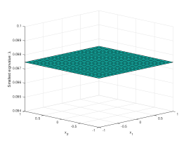
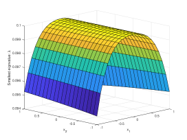
Figure 1. Illustration of convergence rates $\lambda$ with different choices of $\beta$. Left: $\beta=0$; Right $\beta=0.1$.

Example 2 (Variable diffusions).

Consider $U(x)=\frac{x^{2.5}-x}{2.5*1.5}$ with a variable temperature function $r(x)=(\nabla_{xx}U(x))^{-1}$. For simplicity of discussions, we study SDE (22) on a spatial domain $[0.5,1]^{2}$ with periodic boundary conditions. In this case, we can establish convergence rates of SDE (22). Similarly, we plot the smallest eigenvalue $\lambda=\lambda_{\min}((aa^{\mathsf{T}}+zz^{\mathsf{T}})^{-1}\mathfrak{R})$ on a spatial domain $[0.5,1]^{2}$. Here we choose $z=\begin{pmatrix}1\\ 0.1\end{pmatrix}$.

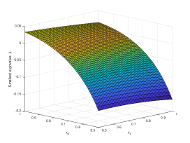
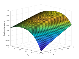
Figure 2. Illustration of convergence rates $\lambda$ with different choices of $\beta$. Left: $\beta=0$; Right: $\beta=0.6$.

Proposition 5 (Sufficient conditions).

In Example $1$, let $\beta=0$, $d=1$, $r(x)=r\in\mathbb{R}_{+}$, then

$$\mathfrak{R} = \begin{pmatrix}z_{1}z_{2}&\frac{1}{2}[{r}z_{1}z_{2}+z_{2}^{2}-\partial^{2}_{xx}Uz_{1}^{2}+r]\\ \frac{1}{2}[{r}z_{1}z_{2}+z_{2}^{2}-\partial^{2}_{xx}Uz_{1}^{2}+r]&r^{2}+{r}z_{2}^{2}-\partial^{2}_{xx}Uz_{1}z_{2}\end{pmatrix}_{2\times 2}.$$

Assume that $\underline{\lambda}\leq\partial_{xx}^{2}U\leq\overline{\lambda}$, and there exist constants $z_{2}\in(0,\frac{r+\sqrt{r^{2}+4r}}{2})$, such that $\underline{\lambda}$, $\overline{\lambda}$ satisfy the following conditions:

$$-\overline{\lambda}^{2}+[2(r(1+z_{2})-z_{2}^{2})]\underline{\lambda}-[(1-z_{2})r+z_{2}^{2}]^{2}>0,\quad r^{2}+rz_{2}^{2}-\overline{\lambda}z_{2}>0.$$ (25)

Then there exists $\lambda>0$, such that

$$\mathfrak{R}\succeq\lambda(aa^{\mathsf{T}}+zz^{\mathsf{T}}).$$

Proof  It is sufficient to prove $\mathsf{det}(\mathfrak{R})>0$ for $z_{1}z_{2}>0$ and $r^{2}+rz_{2}^{2}-\partial^{2}_{xx}Uz_{1}z_{2}>0$, which is equivalent to

$$z_{1}z_{2}(r^{2}+rz_{2}^{2}-\partial^{2}_{xx}Uz_{1}z_{2})-\frac{1}{4}(rz_{1}z_{2}+z_{2}^{2}-\partial^{2}_{xx}Uz_{1}^{2}+r)^{2}>0.$$

It is equivalent to the following inequality:

$$-z_{1}^{4}(\partial_{xx}^{2}U)^{2}+[2(r(1+z_{1}z_{2})-z_{2}^{2})z_{1}^{2}]\partial_{xx}^{2}U-[(1-z_{1}z_{2})r+z_{2}^{2}]^{2}>0.$$ (26)

According to the assumption of $\partial_{xx}^{2}U$, it is sufficient to prove the following conditions:

$$\begin{cases}&z_{1}z_{2}>0,\quad r^{2}+rz_{2}^{2}-\overline{\lambda}z_{1}z_{2}>0,\quad(r(1+z_{1}z_{2})-z_{2}^{2})>0;\\ &-z_{1}^{4}\overline{\lambda}^{2}+[2(r(1+z_{1}z_{2})-z_{2}^{2})z_{1}^{2}]\underline{\lambda}-[(1-z_{1}z_{2})r+z_{2}^{2}]^{2}>0.\end{cases}$$ (27)

Let $z_{1}=1$, then (25) is equivalent to (27). We complete the proof.

Remark 7.

In general, (26) is more general than (27). For example, if we take $z_{1}=1$ and $z_{2}=\frac{r}{2}$, we get

$$-(\partial^{2}_{xx}U)^{2}+2(r+\frac{r^{2}}{4})\partial^{2}_{xx}U-(r-\frac{r^{2}}{4})^{2}>0,\quad r^{2}+\frac{r^{3}}{4}-\partial^{2}_{xx}U\frac{r}{2}>0.$$

The above inequality implies that $r+\frac{r^{2}}{4}-\sqrt{r^{3}}<\partial^{2}_{xx}U<r+\frac{r^{2}}{4}+\sqrt{r^{3}}$, since we also have $r+\frac{r^{2}}{4}+\sqrt{r^{3}}<2r+\frac{r^{2}}{2}$.

4. Example II: $3$-oscillators with nearest-neighbor couplings

In this section, we apply Theorem 1 to prove the exponential convergence in $L_{1}$ distance for three oscillator chains with nearest-neighbor couplings [26]. Consider

$$\left\{\begin{aligned} dq_{j}=&p_{j}dt,\quad j=0,1,2,\\ dp_{0}=&-\xi_{0}p_{0}dt-V^{\prime}_{1}(q_{0})dt-V_{2}^{\prime}(q_{0}-q_{1})dt+\sqrt{2\xi_{0}T}dB_{0},\\ dp_{1}=&-V^{\prime}_{1}(q_{1})dt-V_{2}^{\prime}(q_{1}-q_{0})dt-V_{2}^{\prime}(q_{1}-q_{2})dt,\\ dp_{2}=&-\xi_{2}p_{2}dt-V_{1}^{\prime}(q_{2})dt-V_{2}^{\prime}(q_{2}-q_{1})dt+\sqrt{2\xi_{2}T}dB_{2}.\end{aligned}\right.$$ (28)

We abuse the notation slightly. Denote $q\in\mathbb{R}^{3}$ as the state variable and $p\in\mathbb{T}^{3}$ as the moment variable, where $\mathbb{T}^{3}$ is a $3$ dimensional torus. The dynamics (28) is associated with the Hamiltonian function

$$H(p,q)=\sum_{i=0}^{2}(\frac{{|p_{i}|^{2}}}{2}+V_{1}(q_{i}))+\sum_{i=1}^{2}V_{2}(q_{i}-q_{i-1}),$$

where function $V_{2}$ is a smooth interaction potential between neighboring oscillators, and function $V_{1}$ is a smooth pinning potential. In this paper, we consider $\xi_{0}=\xi_{2}$. We assume that there exists a unique invariant measure $\pi$, where

$$\pi(p,q)=\frac{1}{Z}e^{-\frac{H(p,q)}{T}},$$

with a normalization constant $Z=\int_{\mathbb{R}^{3}\times\mathbb{T}^{3}}e^{-\frac{H(p,q)}{T}}dqdp<\infty$.

Remark 8.

If $\xi_{0}\neq\xi_{2}$, there is no explicit formulation for the invariant density $\pi$. See related studies [20, 21, 26]. This example focuses on the case when $\pi$ is explicitly known.

Notations: Denote $X(t)=(q_{0}(t),q_{1}(t),q_{2}(t),p_{0}(t),p_{1}(t),p_{2}(t))^{\mathsf{T}}$ and $x=(q_{0},q_{1},q_{2},p_{0},p_{1},p_{2})^{\mathsf{T}}$. Equation (28) can be written as

$$dX_{t} = b(X_{t})dt+\sqrt{2}adB_{t},$$

where we write $B_{t}=(B_{0}(t),B_{2}(t))^{\mathsf{T}}$,

$$b(X) = \begin{pmatrix}p_{0}&p_{1}&p_{2}&-\xi p_{0}-\partial_{q_{0}}H&-\partial_{q_{1}}H&-\xi p_{2}-\partial_{q_{2}}H\end{pmatrix}^{\mathsf{T}},$$

and

$$a=\begin{pmatrix}0&0&0&\sqrt{\xi T}&0&0\\ 0&0&0&0&0&\sqrt{\xi T}\end{pmatrix}^{\mathsf{T}}.$$

Denote $\mathsf{I}_{3}=\mathsf{Diag}(1,1,1)_{3\times 3}$ as an identity matrix. We select the matrix $z$ as

$$z=\begin{pmatrix}z_{1}\mathsf{I}_{3}&0_{3\times 1}\\ z_{2}\mathsf{I}_{3}&(\overrightarrow{z_{3}})_{3\times 1}\end{pmatrix}_{6\times 4},$$

where we denote $\overrightarrow{z_{3}}=\begin{pmatrix}z_{31}&z_{32}(p_{0},p_{2})&z_{33}\end{pmatrix}^{\mathsf{T}}$ for constants $z_{31},z_{33}\in\mathbb{R}$, and function $z_{32}(p_{0},p_{2})$, $z_{32}:\mathbb{R}^{2}\rightarrow\mathbb{R}$. We observe that

$$aa^{\mathsf{T}}=\begin{pmatrix}0&0\\ 0&(\xi T)\mathsf{I}_{3}^{O}\end{pmatrix}_{6\times 6},\quad zz^{\mathsf{T}}=\begin{pmatrix}z_{1}^{2}\mathsf{I}_{3}&z_{1}z_{2}\mathsf{I}_{3}\\ z_{1}z_{2}\mathsf{I}_{3}&z_{2}^{2}\mathsf{I}_{3}+\overrightarrow{z_{3}}\overrightarrow{z_{3}}^{\mathsf{T}}\end{pmatrix}_{6\times 6},$$

where we write $\mathsf{I}_{3}^{O}=\mathsf{Diag}(1,0,1)_{3\times 3}$, and

$$\gamma(x) = a(x)a(x)^{\mathsf{T}}\nabla\log\pi(x)-b(x)+\big{(}\sum_{j=1}^{6}\frac{\partial}{\partial x_{j}}(a(x)a(x)^{\mathsf{T}})_{ij}\big{)}_{1\leq i\leq 6}$$

$$= \begin{pmatrix}-p_{0}&-p_{1}&-p_{2}&\partial_{q_{0}}H&\partial_{q_{1}}H&\partial_{q_{2}}H\end{pmatrix}^{\mathsf{T}}.$$

It is easy to verify that $\nabla\cdot(\pi\gamma)=0$. We have the following matrix function $\mathfrak{R}$ for SDE (28).

Proposition 6.

Define a matrix function $\mathfrak{R}\in\mathbb{R}^{6\times 6}$ as

$$\mathfrak{R}=\begin{pmatrix}\mathsf{R}_{1}&\mathsf{R}_{2}\\ \mathsf{R}_{2}&\mathsf{R}_{3}\end{pmatrix}_{6\times 6},$$

with

$$\mathsf{R}_{1} = z_{1}z_{2}\mathsf{I}_{3},\quad\mathsf{R}_{2}=\frac{1}{2}(z_{1}z_{2}\xi+\xi T)\mathsf{I}_{3}^{O}+\frac{1}{2}(z_{2}^{2}\mathsf{I}_{3}+\overrightarrow{z_{3}}\overrightarrow{z_{3}}^{\mathsf{T}}-z_{1}^{2}L),$$

$$\mathsf{R}_{3} = ((\xi T)^{2}+z_{2}^{2}\xi)\mathsf{I}_{3}^{O}-z_{1}z_{2}L+\frac{1}{2}(\overrightarrow{z_{3}^{\mathsf{S}}}\overrightarrow{z_{3}}^{\mathsf{T}}+\overrightarrow{z_{3}}(\overrightarrow{z_{3}^{\mathsf{S}}})^{\mathsf{T}})+\mathsf{I}_{\pi},$$

where we write

$$\mathsf{I}_{3}^{O} = \mathsf{Diag}(1,0,1)_{3\times 3},\quad\overrightarrow{z_{3}^{\mathsf{S}}}=(z_{31}\xi\quad\mathsf{S}_{1}\quad z_{33}\xi)^{\mathsf{T}},$$

$$\mathsf{I}_{\pi} = \begin{pmatrix}0&0&0\\ 0&-2z_{32}\mathsf{S}_{1}-2\xi T[|\partial_{p_{0}}z^{\mathsf{T}}_{45}|^{2}+|\partial_{p_{2}}z^{\mathsf{T}}_{45}|^{2}]&0\\ 0&0&0\end{pmatrix}_{3\times 3},\quad{L=(\nabla^{2}_{q_{i}q_{j}}H)_{0\leq i,j\leq 2}},$$

$$\mathsf{S}_{1} = \xi T\partial_{p_{0}p_{0}}z_{32}+\xi T\partial_{p_{2}p_{2}}z_{32}+(\xi T\partial_{p_{0}}\log\pi)\partial_{p_{0}}z_{32}+(\xi T\partial_{p_{2}}\log\pi)\partial_{p_{2}}z_{32}.$$

If there exists a constant $\lambda>0$, such that

$$\mathfrak{R}\succeq\lambda(aa^{\mathsf{T}}+zz^{\mathsf{T}}),$$

then entropy dissipation results in Theorem 1 and Corollary 2 hold.

To simplify the computation, we choose the following parameters:

$$\xi=T=1,\quad z_{31}=z_{33}=0,\quad z_{32}(p_{0},p_{2})=N-\varepsilon p_{0}^{2}/2,\quad z_{1}=1,$$ (29)

with a fixed constant $N>0$ and a fixed scaling constant $\varepsilon>0$.

Proposition 7 (Sufficient conditions).

Assume that $(\nabla^{2}_{q_{i}q_{j}}H)_{0\leq i,j\leq 2}$ satisfies the following conditions, for $\delta_{1},\delta_{2}>0$, $z_{2}\in(0,\min\{\frac{1+\sqrt{5}}{2},N\})$, and a small constant $\varepsilon>0$,

$$\begin{cases}&\underline{\lambda}\mathsf{I}_{3}\preceq{(\nabla^{2}_{q_{i}q_{j}}H)_{0\leq i,j\leq 2}}\preceq\overline{\lambda}\mathsf{I}_{3};\\ &2\underline{\lambda}-\overline{\lambda}^{2}\geq 1-\delta_{1},\quad-(z_{2}^{2}+N^{2})^{2}+2(N^{2}-z_{2}^{2})\underline{\lambda}-\overline{\lambda}^{2}>0;\\ &2z_{2}+2z_{2}^{3}-z_{2}^{4}-3z_{2}^{2}+2(z_{2}-z_{2}^{2})\underline{\lambda}>\delta_{1}.\end{cases}$$ (30)

We denote $0\leq\underline{\lambda}\leq\overline{\lambda}$ as the lower and upper bounds for the eigenvalues of the matrix $\nabla^{2}_{qq}H$. Then there exists a constant $\lambda>0$, such that

$$\mathfrak{R}\succeq\lambda(aa^{\mathsf{T}}+zz^{\mathsf{T}}).$$

Remark 9.

The condition of $\nabla^{2}_{qq}H$ in the above proposition implies the condition for $\nabla^{2}_{qq}V_{1}$ and $\nabla^{2}_{qq}V_{2}$.

Proof  It is sufficient to prove that $\mathfrak{R}$ defined in Proposition 6 is positive definite. Applying the Schur complement for symmetric matrix function [47][Appendix A.5], the following conditions are equivalent:

• $\mathfrak{R}\succeq 0$ ($\mathfrak{R}$ is positive semidefinite).

• $\mathsf{R}_{1}\succeq 0$, $(\mathsf{I}_{3}-\mathsf{R}_{1}\mathsf{R}_{1}^{-1})\mathsf{R}_{2}=0$, $\mathsf{R}_{3}-\mathsf{R}_{2}\mathsf{R}_{1}^{-1}\mathsf{R}_{2}\succeq 0$.

Plugging in the parameters from (29), and letting $z_{2}>0$, we need to show $\mathsf{R}_{3}-\mathsf{R}_{2}\mathsf{R}_{1}^{-1}\mathsf{R}_{2}\succeq 0$. In other words,

$$\mathsf{R}_{3}-\mathsf{R}_{2}\mathsf{R}_{1}^{-1}\mathsf{R}_{2}$$

$$= \begin{pmatrix}1+z_{2}^{2}&0&0\\ 0&\varepsilon(1-p_{0}^{2})(N-\varepsilon p_{0}^{2}/2)-2\varepsilon^{2}p_{0}^{2}&0\\ 0&0&1+z_{2}^{2}\end{pmatrix}-z_{2}L$$

$$-\frac{1}{z_{2}}\Big{(}\begin{pmatrix}\frac{1}{2}z_{2}^{2}+\frac{1}{2}z_{2}+\frac{1}{2}&0&0\\ 0&\frac{1}{2}z_{2}^{2}+\frac{1}{2}(N-\varepsilon p_{0}^{2}/2)^{2}&0\\ 0&0&\frac{1}{2}z_{2}^{2}+\frac{1}{2}z_{2}+\frac{1}{2}\end{pmatrix}-\frac{1}{2}L\Big{)}^{2}$$

$$:= \mathsf{Diag}(C_{1},C_{2},C_{3})-z_{2}\mathsf{O}\cdot\mathsf{Diag}(\lambda_{1},\lambda_{2},\lambda_{3})_{3\times 3}\cdot\mathsf{O}^{\mathsf{T}}$$

$$-\frac{1}{4z_{2}}\Big{(}\mathsf{Diag}(C_{4},C_{5},C_{6})-\mathsf{O}\cdot\mathsf{Diag}(\lambda_{1},\lambda_{2},\lambda_{3})_{3\times 3}\cdot\mathsf{O}^{\mathsf{T}}\Big{)}^{2},$$

where

$$C_{1} = C_{3}=1+z_{2}^{2},\quad C_{2}=\varepsilon(1-p_{0}^{2})(N-\varepsilon p_{0}^{2}/2)-2\varepsilon^{2}p_{0}^{2},\quad$$

$$C_{4} = C_{6}=1+z_{2}^{2}+z_{2},\quad C_{5}=z_{2}^{2}+(N-\varepsilon p_{0}^{2}/2)^{2},$$

and we denote the eigenvalue decomposition of matrix $L$ as

$$L=\mathsf{O}\cdot\mathsf{Diag}(\lambda_{1},\lambda_{2},\lambda_{3})_{3\times 3}\cdot\mathsf{O}^{\mathsf{T}}.$$

We write $\mathsf{O}\in\mathbb{R}^{3\times 3}$ as the orthogonal matrix with $\mathsf{O}^{-1}=\mathsf{O}^{\mathsf{T}}$ and $\lambda_{1}\leq\lambda_{2}\leq\lambda_{3}$ as the eigenvalues of matrix $L$. Thus

$$\mathsf{R}_{3}-\mathsf{R}_{2}\mathsf{R}_{1}^{-1}\mathsf{R}_{2}$$

$$= \mathsf{O}\cdot\mathsf{Diag}\Big{(}\Big{(}C_{i}-z_{2}\lambda_{i}-\frac{1}{4z_{2}}(C_{i+3}^{2}-2C_{i+3}\lambda_{i}+\lambda^{2}_{i})\Big{)}_{1\leq i\leq 3}\Big{)}_{3\times 3}\cdot\mathsf{O}^{\mathsf{T}}$$

$$= \mathsf{O}\cdot\mathsf{Diag}\Big{(}\Big{(}C_{i}-\frac{C_{i+3}^{2}}{4z_{2}}+(\frac{C_{i+3}}{2z_{2}}-z_{2})\lambda_{i}-\frac{\lambda^{2}_{i}}{4z_{2}}\Big{)}_{1\leq i\leq 3}\Big{)}_{3\times 3}\cdot\mathsf{O}^{\mathsf{T}}$$

It is sufficient to find parameters $z_{2}$, $N$, and $\varepsilon$, such that the following inequalities hold:

$$\Big{(}C_{i}-\frac{C_{i+3}^{2}}{4z_{2}}+(\frac{C_{i+3}}{2z_{2}}-z_{2})\lambda_{i}-\frac{\lambda^{2}_{i}}{4z_{2}}\Big{)}>0,\quad 1\leq i\leq 3.$$

Since $z_{2}>0$, it is equivalent to prove

$$\begin{cases}z_{2}(1+z_{2}^{2})-\frac{(1+z_{2}+z_{2}^{2})^{2}}{4}+(\frac{1+z_{2}+z_{2}^{2}}{2}-z_{2}^{2})\lambda_{i}-\frac{\lambda^{2}_{i}}{4}>0,\\ z_{2}\varepsilon(1-p_{0}^{2})(N-\varepsilon p_{0}^{2}/2)-2\varepsilon^{2}p_{0}^{2}-\frac{(z_{2}^{2}+(N-\varepsilon p_{0}^{2}/2)^{2})^{2}}{4}+(\frac{z_{2}^{2}+(N-\varepsilon p_{0}^{2}/2)^{2}}{2}-z_{2}^{2})\lambda_{i}-\frac{\lambda^{2}_{i}}{4}>0.\end{cases}$$ (31)

The first inequality in (31) holds under the following conditions. Suppose $1+z_{2}-z_{2}^{2}>0$,

$$2\underline{\lambda}-\overline{\lambda}^{2}\geq 1-\delta_{1},\qquad 2z_{2}+2z_{2}^{3}-z_{2}^{4}-3z_{2}^{2}+2(z_{2}-z_{2}^{2})\underline{\lambda}>\delta_{1}.$$

For $p_{0}\in\mathbb{T}^{1}$, we select $\varepsilon$ to be very small, such that

$$-\frac{(z_{2}^{2}+N^{2})^{2}}{4}+(N^{2}-z_{2}^{2})\frac{\underline{\lambda}}{2}-\frac{\overline{\lambda}^{2}}{4}>0.$$

The proof is finished.  

Remark 10.

Consider $\underline{\lambda}=0.6$, $\overline{\lambda}=0.65$, $N=1$, $z_{2}=0.2$, $\delta_{1}=0.225$, $\varepsilon=10^{-7}$. All conditions in (30) are satisfied.

Remark 11.

In the current paper, we restrict $p\in\mathbb{T}^{3}$, which differs from the setting in [26]. We mainly use the torus property to construct the matrix $z$, i.e. $z_{32}(p_{0},p_{2})$ in (29), such that we can establish the desired bounds in Proposition 7. We leave the general setting with $p\in\mathbb{R}^{3}$ for future studies.

5. Proof

In this section, we present the main proofs of this paper.

5.1. Outline of main results

Before showing all the detailed proofs in Theorem 1, we outline the main ideas in the following three steps. We postpone all derivations to subsection 5.3.

• We first compute the dissipation of the weighted Fisher information functional.

  $$\frac{d}{dt}\mathcal{I}_{a,z}(p\|\pi)=-2\int\Gamma_{2,a,z,\gamma}(f,f)pdx,$$

  where $f=\log\frac{p}{\pi}$ and

  $$\Gamma_{2,a,z,\gamma}(f,f)=\widetilde{\Gamma}_{2}(f,f)+\widetilde{\Gamma}_{2}^{z,\pi}(f,f)+\Gamma_{\mathcal{I}_{a,z}}(f,f).$$

  The definition of the above operators will be introduced shortly in Definition 2.

• We next decompose the weak form of information Gamma calculus. This is to derive the information Bochner’s formula (Theorem 3):

  $$\int\Gamma_{2,a,z,\gamma}(f,f)pdx=\int\Big{[}\|\mathfrak{Hess}_{\beta}f\|_{\mathrm{F}}^{2}+\mathfrak{R}(\nabla f,\nabla f)\Big{]}pdx.$$

• From the information Bochner’s formula, we establish the convergence result. In other words, if $\mathfrak{R}\succeq\lambda(aa^{\mathsf{T}}+zz^{\mathsf{T}})$, then

  $$\frac{d}{dt}\mathcal{I}_{a,z}(p\|\pi)\leq-2\lambda\mathcal{I}_{a,z}(p\|\pi).$$

  From Gronwall’s inequality, we can prove that the weighted Fisher information decays in Theorem 1. This decay result also establishes other functionals decay in Corollary 2.

We remark that Step $1$ is based on a global in-space computation, which comes from the second-order calculus of entropy functional in the sub-Riemannian density manifold. We carefully handle the non-communicative operators based on $\Gamma_{1}$, $\Gamma_{1}^{z}$, and vector field $\gamma$. Step $2$ is a local in-space calculation, which can be viewed as a generalization of Bochner’s formula. Step $3$ follows directly from the modified Lyapunov method.

5.2. Information Gamma calculus

We next introduce all tensors for the main proof. These tensors are derived from the information Gamma calculus. Denote the following operators of SDE (1). For any $f\in C^{\infty}(\mathbb{R}^{n+m})$, the generator of SDE (1) satisfies

$$Lf=\widetilde{L}f-\langle\gamma,\nabla f\rangle,$$

where

$$\widetilde{L}f = \nabla\cdot(aa^{\mathsf{T}}\nabla f)+\langle aa^{\mathsf{T}}\nabla\log\pi,\nabla f\rangle,$$ (32)

is the reversible component of the Kolmogorov backward operator. For a given matrix function $a\in\mathbb{R}^{(n+m)\times n}$, we construct a matrix function $z\in\mathbb{R}^{(n+m)\times m}$ to handle the degenerate component of SDE (1). We also denote a $z$-direction generator as

$$\widetilde{L}_{z}f=\nabla\cdot(zz^{\mathsf{T}}\nabla f)+\langle zz^{\mathsf{T}}\nabla\log\pi,\nabla f\rangle.$$

Define Gamma one bilinear forms $\Gamma_{1},\Gamma_{1}^{z}\colon C^{\infty}(\mathbb{R}^{n+m})\times C^{\infty}(\mathbb{R}^{n+m})\rightarrow C^{\infty}(\mathbb{R}^{n+m})$ as

$$\Gamma_{1}(f,f)=\langle a^{\mathsf{T}}\nabla f,a^{\mathsf{T}}\nabla f\rangle_{\mathbb{R}^{n}},\quad\Gamma_{1}^{z}(f,f)=\langle z^{\mathsf{T}}\nabla f,z^{\mathsf{T}}\nabla f\rangle_{\mathbb{R}^{m}}.$$ (33)

We now define the information Gamma operators for SDE (1). In fact, it is a derivative calculation based on the reversible Kolmogorov backward operator $\widetilde{L}$, the non-reversible vector field $\gamma$, and the invariant distribution $\pi$.

Definition 2 (Information Gamma operators).

Define the following three bi-linear forms:

$$\widetilde{\Gamma}_{2},\widetilde{\Gamma}_{2}^{z,\pi},\Gamma_{\mathcal{I}_{a,z}}\colon C^{\infty}(\mathbb{R}^{n+m})\times C^{\infty}(\mathbb{R}^{n+m})\rightarrow C^{\infty}(\mathbb{R}^{n+m}).$$

• Gamma two operator:

  $$\widetilde{\Gamma}_{2}(f,f)=\frac{1}{2}\widetilde{L}\Gamma_{1}(f,f)-\Gamma_{1}(\widetilde{L}f,f).$$

• Generalized Gamma $z$ operator:

  $$\widetilde{\Gamma}_{2}^{z,\pi}(f,f) = \quad\frac{1}{2}\widetilde{L}\Gamma_{1}^{z}(f,f)-\Gamma_{1}^{z}(\widetilde{L}f,f)$$

  $$+\mathbf{div}^{{\pi}}_{z}\Big{(}\Gamma_{1,\nabla(aa^{\mathsf{T}})}(f,f)\Big{)}-\mathbf{div}^{{\pi}}_{a}\Big{(}\Gamma_{1,\nabla(zz^{\mathsf{T}})}(f,f)\Big{)}.$$

  Here $\mathbf{div}^{{\pi}}_{a}$, $\mathbf{div}^{{\pi}}_{z}$ are divergence operators defined by

  $$\mathbf{div}^{{\pi}}_{a}(F)=\frac{1}{{\pi}}\nabla\cdot({\pi}aa^{\mathsf{T}}F),\quad\mathbf{div}^{{\pi}}_{z}(F)=\frac{1}{{\pi}}\nabla\cdot({\pi}zz^{\mathsf{T}}F),$$

  for any smooth vector field $F\in\mathbb{R}^{n+m}$, and $\Gamma_{1,\nabla(aa^{\mathsf{T}})}$, $\Gamma_{1,\nabla(zz^{\mathsf{T}})}$ are vector Gamma one bilinear forms defined by

  $$\Gamma_{1,\nabla(aa^{\mathsf{T})}}(f,f) = \langle\nabla f,\nabla(aa^{\mathsf{T}})\nabla f\rangle=(\langle\nabla f,\frac{\partial}{\partial x_{\hat{k}}}(aa^{\mathsf{T}})\nabla f\rangle)_{\hat{k}=1}^{n+m},$$

  $$\Gamma_{1,\nabla(zz^{\mathsf{T})}}(f,f) = \langle\nabla f,\nabla(aa^{\mathsf{T}})\nabla f\rangle=(\langle\nabla f,\frac{\partial}{\partial x_{\hat{k}}}(zz^{\mathsf{T}})\nabla f\rangle)_{\hat{k}=1}^{n+m}.$$

• Irreversible Gamma operator:

  $$\Gamma_{\mathcal{I}_{a,z}}(f,f) = (\widetilde{L}f+\widetilde{L}_{z}f)\langle\nabla f,\gamma\rangle-\frac{1}{2}\langle\nabla\big{(}\Gamma_{1}(f,f)+\Gamma_{1}^{z}(f,f)\big{)},\gamma\rangle.$$

Under Assumption 1, we establish the following information Bochner’s formula.

Theorem 3 (Information Bochner’s formula).

If Assumption 1 is satisfied, then the following decomposition holds. For any $f=\log\frac{p}{\pi}\in C^{\infty}(\mathbb{R}^{n+m},\mathbb{R})$ and any $\beta\in\mathbb{R}$,

$$\int\Big{[}\widetilde{\Gamma}_{2}(f,f)+\widetilde{\Gamma}_{2}^{z,\pi}(f,f)+\Gamma_{\mathcal{I}_{a,z}}(f,f)\Big{]}pdx=\int\Big{[}\|\mathfrak{Hess}_{\beta}f\|_{\mathrm{F}}^{2}+\mathfrak{R}(\nabla f,\nabla f)\Big{]}pdx.$$

We denote

$$\|\mathfrak{Hess}_{\beta}f\|_{\mathrm{F}}^{2}=[\mathsf{Q}\mathsf{X}+\Lambda_{1}]^{\mathsf{T}}[\mathsf{Q}\mathsf{X}+\Lambda_{1}]+[\mathsf{P}\mathsf{X}+\Lambda_{2}]^{\mathsf{T}}[\mathsf{P}\mathsf{X}+\Lambda_{2}],$$

where $\mathfrak{R}$, $\Lambda_{1}$, $\Lambda_{2}$ are defined in Definition 1. And we define matrices $\mathsf{Q}$ and $\mathsf{P}$ by

$$\mathsf{Q}=a^{\mathsf{T}}\otimes a^{\mathsf{T}}\in\mathbb{R}^{n^{2}\times(n+m)^{2}},\quad\mathsf{P}=a^{\mathsf{T}}\otimes z^{\mathsf{T}}\in\mathbb{R}^{(nm)\times(n+m)^{2}},$$ (34)

with $\mathsf{Q}_{ik\hat{i}\hat{k}}=a^{\mathsf{T}}_{i\hat{i}}a^{\mathsf{T}}_{k\hat{k}}$ and $\mathsf{P}_{ik\hat{i}\hat{k}}=a^{\mathsf{T}}_{i\hat{i}}z^{\mathsf{T}}_{k\hat{k}}$. More precisely, for each row (resp. column) of $\mathsf{Q}$, the row (resp. column) indices of $\mathsf{Q}_{ik\hat{i}\hat{k}}$ follow the double summation $\sum_{i=1}^{n}\sum_{k=1}^{n}$ (resp. $\sum_{\hat{i}=1}^{n+1}\sum_{\hat{k}=1}^{n+m}$). For any smooth function $f:\mathbb{R}^{n+m}\rightarrow\mathbb{R}$, we define $\mathsf{X}\in\mathbb{R}^{(n+m)^{2}\times 1}$ by the vectorization of the Hessian matrix for function $f$ with

$$\mathsf{X}_{\hat{i}\hat{k}}=\frac{\partial^{2}f}{\partial x_{\hat{i}}\partial x_{\hat{k}}},\quad\textrm{for $\hat{i},\hat{k}=1,\cdots,n+m$.}$$

Remark 12 (Optimal Bochner’s formula).

We remark that the proposed information Bochner’s formula can be asymmetric, which could be formulated into a more symmetric way. In other words, denote a quadratic matrix function by

$$\mathcal{F}(Y)=[\mathsf{Q}\mathsf{Y}+\Lambda_{1}]^{\mathsf{T}}[\mathsf{Q}\mathsf{Y}+\Lambda_{1}]+[\mathsf{P}\mathsf{Y}+\Lambda_{2}]^{\mathsf{T}}[\mathsf{P}\mathsf{Y}+\Lambda_{2}],$$

where $Y\in\mathbb{R}^{(n+m)^{2}\times 1}$ is a vectorization of a symmetric matrix. We next consider a symmetric matrix optimization problem by

$$Y^{*}=\arg\min_{Y}\mathcal{F}(Y).$$

Then a Bochner’s formula forms

$$\begin{split}&\|\mathfrak{Hess}_{\beta}f\|^{2}_{\mathrm{F}}+\mathfrak{R}(\nabla f,\nabla f)\\ =&\mathcal{F}(X)-\mathcal{F}(Y^{*})+\mathcal{F}(Y^{*})+\mathfrak{R}(\nabla f,\nabla f).\end{split}$$

We may call the term $\mathcal{F}(X)-\mathcal{F}(Y^{*})$ the “squared Hessian formula” while name the term $\mathcal{F}(Y^{*})+\mathfrak{R}(\nabla f,\nabla f)+\mathfrak{R}_{\mathcal{I}}(\nabla f,\nabla f)$ the “Ricci curvature type tensor”. This optimal choice of Bochner’s formula is left for future works. See Remark 14 in the Appendix for an example of the optimal Bochner’s formula.

5.3. Proof of Step 1.

Proposition 8.

The following equality holds.

$$\frac{d}{dt}\mathcal{I}_{a,z}(p\|\pi)=-2\int\Gamma_{2,a,z,\gamma}(\log\frac{p}{\pi},\log\frac{p}{\pi})pdx,$$

where $p$ is the solution of Fokker-Planck equation (2).

Proof  The proof combines calculations in [22, 23]. We first present the outline of the proof here. Denote

$$\mathcal{I}_{a,z}(p\|\pi)=\mathcal{I}_{a}(p\|\pi)+\mathcal{I}_{z}(p\|\pi),$$

where

$$\mathcal{I}_{a}(p\|\pi)=\int(\nabla\log\frac{p}{\pi},aa^{\mathsf{T}}\nabla\log\frac{p}{\pi})pdx,\quad\mathcal{I}_{z}(p\|\pi)=\int(\nabla\log\frac{p}{\pi},zz^{\mathsf{T}}\nabla\log\frac{p}{\pi})pdx.$$

We observe the following facts.

Claim $0$:

$$\frac{d}{dt}\mathcal{I}_{a}(p\|\pi)=-2\int\Big{(}\widetilde{\Gamma}_{2}+\Gamma_{\mathcal{I}_{a}}\Big{)}(\log\frac{p}{\pi},\log\frac{p}{\pi})pdx,$$

and

$$\frac{d}{dt}\mathcal{I}_{z}(p\|\pi)=-2\int\Big{(}\widetilde{\Gamma}_{2}^{z,\pi}+\Gamma_{\mathcal{I}_{z}}\Big{)}(\log\frac{p}{\pi},\log\frac{p}{\pi})pdx.$$

From the Claim $0$, we obtain

$$\frac{d}{dt}\mathcal{I}_{a,z}(p\|\pi)=\frac{d}{dt}\mathcal{I}_{a}(p\|\pi)+\frac{d}{dt}\mathcal{I}_{z}(p\|\pi)=-2\int\Gamma_{2,a,z,\gamma}(\log\frac{p}{\pi},\log\frac{p}{\pi})pdx,$$

which finishes the proof. Next, we prove Claim $0$ in details. Denote that $p$ solves the Fokker-Planck equation (2) and let $\tilde{L}^{*}$ be the forward Kolmogorov operator.

Firstly, the dissipation of $\mathcal{I}_{a}(p\|\pi)$ follows

$$\begin{split}&\frac{d}{dt}\mathcal{I}_{a}(p\|\pi)\\ =&\frac{d}{dt}\int\Gamma_{1}(\log\frac{p}{\pi},\log\frac{p}{\pi})pdx\\ =&\int\Gamma_{1}(\log\frac{p}{\pi},\log\frac{p}{\pi})\partial_{t}p+2\Gamma_{1}(\partial_{t}\log\frac{p}{\pi},\log\frac{p}{\pi})pdx\\ =&\int\Gamma_{1}(\log\frac{p}{\pi},\log\frac{p}{\pi})\partial_{t}p+2\Gamma_{1}(\frac{\partial_{t}p}{p},\log\frac{p}{\pi})pdx\\ =&\int\Gamma_{1}(\log\frac{p}{\pi},\log\frac{p}{\pi})\partial_{t}p-2\frac{\nabla\cdot(paa^{\mathsf{T}}\nabla\log\frac{p}{\pi})}{p}\partial_{t}pdx\\ =&\int\Gamma_{1}(\log\frac{p}{\pi},\log\frac{p}{\pi})\partial_{t}p-2\Big{(}\langle\nabla\log p,aa^{\mathsf{T}}\nabla\log\frac{p}{\pi}\rangle+\nabla\cdot(aa^{\mathsf{T}}\nabla\log\frac{p}{\pi})\Big{)}\partial_{t}pdx\end{split}$$

$$\begin{split}=&\int\Gamma_{1}(\log\frac{p}{\pi},\log\frac{p}{\pi})\partial_{t}p-2\Big{(}\langle\nabla\log\frac{p}{\pi},aa^{\mathsf{T}}\nabla\log\frac{p}{\pi}\rangle+\widetilde{L}\log\frac{p}{\pi}\Big{)}\partial_{t}pdx\\ =&-2\int\Big{\{}\frac{1}{2}\Gamma_{1}(\log\frac{p}{\pi},\log\frac{p}{\pi})\partial_{t}p+\widetilde{L}\log\frac{p}{\pi}\partial_{t}p\Big{\}}dx\\ =&-2\int\Big{\{}\quad\frac{1}{2}\Gamma_{1}(\log\frac{p}{\pi},\log\frac{p}{\pi})\nabla\cdot(p\gamma)+\widetilde{L}\log\frac{p}{\pi}\nabla\cdot(p\gamma)\\ &\hskip 42.67912pt+\frac{1}{2}\Gamma_{1}(\log\frac{p}{\pi},\log\frac{p}{\pi})\widetilde{L}^{*}p+\widetilde{L}\log\frac{p}{\pi}\widetilde{L}^{*}p\Big{\}}dx\\ =&-2\int\Big{\{}-\frac{1}{2}\langle\nabla\Gamma_{1}(\log\frac{p}{\pi},\log\frac{p}{\pi}),\gamma\rangle+\widetilde{L}\log\frac{p}{\pi}\langle\nabla\log\frac{p}{\pi},\gamma\rangle\\ &\hskip 42.67912pt+\frac{1}{2}\widetilde{L}\Gamma_{1}(\log\frac{p}{\pi},\log\frac{p}{\pi})-\Gamma_{1}(\widetilde{L}\log\frac{p}{\pi},\log\frac{p}{\pi})\Big{\}}pdx\\ =&-2\int\Big{\{}\Gamma_{\mathcal{I}_{a}}(\log\frac{p}{\pi},\log\frac{p}{\pi})+\widetilde{\Gamma}_{2}(\log\frac{p}{\pi},\log\frac{p}{\pi})\Big{\}}pdx.\end{split}$$

In above derivations, we apply the following fact:

$$\nabla\cdot(p\gamma)=p\Big{(}\langle\nabla\log p,\gamma\rangle+\nabla\cdot\gamma\Big{)}=p\langle\nabla\log\frac{p}{\pi},\gamma\rangle,$$

where we use the identity $\nabla\cdot(\pi\gamma)=\pi\Big{(}\langle\nabla\log\pi,\gamma\rangle+\nabla\cdot\gamma\Big{)}=0$.

Secondly, we compute the dissipation of $\mathcal{I}_{z}(p\|\pi)$. Denote

$$\widetilde{L}_{z}=(\nabla\log\pi,zz^{\mathsf{T}}\nabla)+\nabla\cdot(zz^{\mathsf{T}}\nabla).$$

Hence

$$\begin{split}&\frac{d}{dt}\mathcal{I}_{z}(p\|\pi)\\ =&\frac{d}{dt}\int\Gamma_{1}^{z}(\log\frac{p}{\pi},\log\frac{p}{\pi})pdx\\ =&\int\Gamma_{1}^{z}(\log\frac{p}{\pi},\log\frac{p}{\pi})\partial_{t}p+2\Gamma_{1}^{z}(\partial_{t}\log\frac{p}{\pi},\log\frac{p}{\pi})pdx\\ =&\int\Gamma_{1}^{z}(\log\frac{p}{\pi},\log\frac{p}{\pi})\partial_{t}p+2\Gamma_{1}^{z}(\frac{\partial_{t}p}{p},\log\frac{p}{\pi})pdx\\ =&\int\Gamma_{1}^{z}(\log\frac{p}{\pi},\log\frac{p}{\pi})\partial_{t}p-2\frac{\nabla\cdot(pzz^{\mathsf{T}}\nabla\log\frac{p}{\pi})}{p}\partial_{t}pdx\\ =&\int\Gamma_{1}^{z}(\log\frac{p}{\pi},\log\frac{p}{\pi})\partial_{t}p-2\Big{(}\langle\nabla\log p,zz^{\mathsf{T}}\nabla\log\frac{p}{\pi}\rangle+\nabla\cdot(zz^{\mathsf{T}}\nabla\log\frac{p}{\pi})\Big{)}\partial_{t}pdx\\ =&\int\Gamma_{1}^{z}(\log\frac{p}{\pi},\log\frac{p}{\pi})\partial_{t}p-2\Big{(}\langle\nabla\log\frac{p}{\pi},zz^{\mathsf{T}}\nabla\log\frac{p}{\pi}\rangle+\widetilde{L}_{z}\log\frac{p}{\pi}\Big{)}\partial_{t}pdx\end{split}$$

$$\begin{split}=&-2\int\Big{\{}\frac{1}{2}\Gamma_{1}^{z}(\log\frac{p}{\pi},\log\frac{p}{\pi})\partial_{t}p+\widetilde{L}_{z}\log\frac{p}{\pi}\partial_{t}p\Big{\}}dx\\ =&-2\int\Big{\{}\quad\frac{1}{2}\Gamma_{1}^{z}(\log\frac{p}{\pi},\log\frac{p}{\pi})\nabla\cdot(p\gamma)+\widetilde{L}_{z}\log\frac{p}{\pi}\nabla\cdot(p\gamma)\\ &\hskip 42.67912pt+\frac{1}{2}\Gamma_{1}^{z}(\log\frac{p}{\pi},\log\frac{p}{\pi})\widetilde{L}^{*}p+\widetilde{L}_{z}\log\frac{p}{\pi}\widetilde{L}^{*}p\Big{\}}dx\\ =&-2\int\Big{\{}\Gamma_{\mathcal{I}_{z}}(\log\frac{p}{\pi},\log\frac{p}{\pi})+\frac{1}{2}\widetilde{L}_{z}\Gamma_{1}(\log\frac{p}{\pi},\log\frac{p}{\pi})-\Gamma_{1}(\widetilde{L}_{z}\log\frac{p}{\pi},\log\frac{p}{\pi})\Big{\}}pdx.\end{split}$$

We note that the above formula can not be used to derive Bochner’s formula. Since the related third derivative tensors can not be eliminated. To handle this issue, we present the following equality

$$\int\Big{\{}\frac{1}{2}\widetilde{L}_{z}\Gamma_{1}(\log\frac{p}{\pi},\log\frac{p}{\pi})-\Gamma_{1}(\widetilde{L}_{z}\log\frac{p}{\pi},\log\frac{p}{\pi})\Big{\}}pdx=\int\widetilde{\Gamma}_{2}^{z,\pi}(\log\frac{p}{\pi},\log\frac{p}{\pi})pdx.$$ (35)

The identity (35) has been derived in [22, Proposition $5.11$]. For completeness of this paper, we also present its derivation here. Notice that

$$\begin{split}&\frac{1}{2}\widetilde{L}_{z}\Gamma_{1}(\log\frac{p}{\pi},\log\frac{p}{\pi})-\Gamma_{1}(\widetilde{L}_{z}\log\frac{p}{\pi},\log\frac{p}{\pi})\\ =&\frac{1}{2}\widetilde{L}_{z}\Gamma_{1}(\log\frac{p}{\pi},\log\frac{p}{\pi})-\Gamma_{1}^{z}(\widetilde{L}\log\frac{p}{\pi},\log\frac{p}{\pi})+\Gamma_{1}^{z}(\widetilde{L}\log\frac{p}{\pi},\log\frac{p}{\pi})-\Gamma_{1}(\widetilde{L}_{z}\log\frac{p}{\pi},\log\frac{p}{\pi}).\end{split}$$

We next claim that

$$\begin{split}&\int\Big{\{}\Gamma_{1}^{z}(\widetilde{L}\log\frac{p}{\pi},\log\frac{p}{\pi})-\Gamma_{1}(\widetilde{L}_{z}\log\frac{p}{\pi},\log\frac{p}{\pi})\Big{\}}pdx\\ =&\int\Big{\{}\mathbf{div}^{{\pi}}_{z}\Big{(}\Gamma_{1,\nabla(aa^{\mathsf{T}})}(\log\frac{p}{\pi},\log\frac{p}{\pi})\Big{)}-\mathbf{div}^{{\pi}}_{a}\Big{(}\Gamma_{1,\nabla(zz^{\mathsf{T}})}(\log\frac{p}{\pi},\log\frac{p}{\pi})\Big{)}\Big{\}}pdx.\end{split}$$

We derive it as follows. Firstly,

$$\begin{split}&\int\Gamma_{1}^{z}(\widetilde{L}\log\frac{p}{\pi},\log\frac{p}{\pi})pdx\\ =&\int\Gamma_{1}^{z}\Big{(}\langle\nabla\log\pi,aa^{\mathsf{T}}\nabla\log\frac{p}{\pi}\rangle+\nabla\cdot(aa^{\mathsf{T}}\nabla\log\frac{p}{\pi}),\log\frac{p}{\pi}\Big{)}pdx\\ =&\int\Gamma_{1}^{z}\Big{(}\Gamma_{1}(\log\pi,\log\frac{p}{\pi}),\log\frac{p}{\pi}\Big{)}p+\Gamma_{1}^{z}\Big{(}\nabla\cdot(aa^{\mathsf{T}}\nabla\log\frac{p}{\pi}),\log\frac{p}{\pi}\Big{)}pdx\\ =&\int\Gamma_{1}^{z}\Big{(}\Gamma_{1}(\log\pi,\log\frac{p}{\pi}),\log\frac{p}{\pi}\Big{)}pdx-\int\nabla\cdot(aa^{\mathsf{T}}\nabla\log\frac{p}{\pi})\nabla\cdot(pzz^{\mathsf{T}}\nabla\log\frac{p}{\pi})dx.\end{split}$$

We note that the second term in the above formula can be written below.

$$\begin{split}&-\int\nabla\cdot(aa^{\mathsf{T}}\nabla\log\frac{p}{\pi})\nabla\cdot(pzz^{\mathsf{T}}\nabla\log\frac{p}{\pi})dx\\ =&-\int\nabla\cdot(\frac{\pi}{p}aa^{\mathsf{T}}\nabla\frac{p}{\pi})\nabla\cdot(pzz^{\mathsf{T}}\nabla\log\frac{p}{\pi})dx\\ =&-\int\Big{(}\pi\langle\nabla\frac{1}{p},aa^{\mathsf{T}}\nabla\frac{p}{\pi}\rangle+\frac{1}{p}\nabla\cdot(\pi aa^{\mathsf{T}}\nabla\frac{p}{\pi})\Big{)}\nabla\cdot(pzz^{\mathsf{T}}\nabla\log\frac{p}{\pi})dx\\ =&-\int\pi\langle\nabla\frac{1}{p},aa^{\mathsf{T}}\nabla\frac{p}{\pi}\rangle\nabla\cdot(pzz^{\mathsf{T}}\nabla\log\frac{p}{\pi})dx-\int\frac{1}{p}\nabla\cdot(\pi aa^{\mathsf{T}}\nabla\frac{p}{\pi})\nabla\cdot(\pi zz^{\mathsf{T}}\nabla\frac{p}{\pi})dx\\ =&\int\frac{\pi}{p^{2}}\langle\nabla p,aa^{\mathsf{T}}\nabla\frac{p}{\pi}\rangle\nabla\cdot(pzz^{\mathsf{T}}\nabla\log\frac{p}{\pi})-\frac{1}{p}\nabla\cdot(\pi aa^{\mathsf{T}}\nabla\frac{p}{\pi})\nabla\cdot(\pi zz^{\mathsf{T}}\nabla\frac{p}{\pi})dx\\ =&\int\langle\nabla\log p,aa^{\mathsf{T}}\nabla\log\frac{p}{\pi}\rangle\nabla\cdot(pzz^{\mathsf{T}}\nabla\log\frac{p}{\pi})-\frac{1}{p}\nabla\cdot(\pi aa^{\mathsf{T}}\nabla\frac{p}{\pi})\nabla\cdot(\pi zz^{\mathsf{T}}\nabla\frac{p}{\pi})dx\\ =&\int\Big{\{}\langle\nabla\log\frac{p}{\pi},aa^{\mathsf{T}}\nabla\log\frac{p}{\pi}\rangle\nabla\cdot(pzz^{\mathsf{T}}\nabla\log\frac{p}{\pi})+\langle\nabla\log\pi,aa^{\mathsf{T}}\nabla\log\frac{p}{\pi}\rangle\nabla\cdot(pzz^{\mathsf{T}}\nabla\log\frac{p}{\pi})\\ &\qquad-\frac{1}{p}\nabla\cdot(\pi aa^{\mathsf{T}}\nabla\frac{p}{\pi})\nabla\cdot(\pi zz^{\mathsf{T}}\nabla\frac{p}{\pi})\Big{\}}dx\\ =&\int\Big{\{}-\Gamma_{1}^{z}(\Gamma_{1}(\log\frac{p}{\pi},\log\frac{p}{\pi}),\log\frac{p}{\pi})-\Gamma_{1}^{z}(\Gamma_{1}(\log\pi,\log\frac{p}{\pi}),\log\frac{p}{\pi})p\\ &\qquad-\frac{1}{p}\nabla\cdot(\pi aa^{\mathsf{T}}\nabla\frac{p}{\pi})\nabla\cdot(\pi zz^{\mathsf{T}}\nabla\frac{p}{\pi})\Big{\}}dx\\ =&\int\Big{\{}-\Gamma_{1}^{z}(\Gamma_{1}(\log\frac{p}{\pi},\log\frac{p}{\pi}),\log\frac{p}{\pi})p-\Gamma_{1}^{z}(\Gamma_{1}(\log\pi,\log\frac{p}{\pi}),\log\frac{p}{\pi})p\\ &\qquad-\frac{1}{p}\nabla\cdot(\pi aa^{\mathsf{T}}\nabla\frac{p}{\pi})\nabla\cdot(\pi zz^{\mathsf{T}}\nabla\frac{p}{\pi})\Big{\}}dx.\end{split}$$

We observe that

$$\begin{split}&-\int\Gamma_{1}^{z}(\Gamma_{1}(\log\frac{p}{\pi},\log\frac{p}{\pi}),\log\frac{p}{\pi})pdx\\ =&-\int\nabla^{2}\log\frac{p}{\pi}(aa^{\mathsf{T}}\nabla\log\frac{p}{\pi},zz^{\mathsf{T}}\nabla\log\frac{p}{\pi})pdx\\ &-\int\Big{(}\Gamma_{1,\nabla(aa^{\mathsf{T}})}(\nabla\log\frac{p}{\pi},\nabla\log\frac{p}{\pi})zz^{\mathsf{T}}\nabla\log\frac{p}{\pi}\Big{)}pdx\\ =&-\int\nabla^{2}\log\frac{p}{\pi}(aa^{\mathsf{T}}\nabla\log\frac{p}{\pi},zz^{\mathsf{T}}\nabla\log\frac{p}{\pi})pdx\\ &-\int\Big{(}\Gamma_{1,\nabla(aa^{\mathsf{T}})}(\nabla\log\frac{p}{\pi},\nabla\log\frac{p}{\pi})zz^{\mathsf{T}}\nabla\frac{p}{\pi}\Big{)}\pi dx\\ =&-\int\nabla^{2}\log\frac{p}{\pi}(aa^{\mathsf{T}}\nabla\log\frac{p}{\pi},zz^{\mathsf{T}}\nabla\log\frac{p}{\pi})pdx\\ &+\int\frac{1}{\pi}\nabla\cdot\Big{(}zz^{\mathsf{T}}\Gamma_{1,\nabla(aa^{\mathsf{T}})}(\nabla\log\frac{p}{\pi},\nabla\log\frac{p}{\pi})\Big{)}dx.\end{split}$$

Combining the above three formulas, we have

$$\begin{split}&\int\Gamma_{1}^{z}(\widetilde{L}\log\frac{p}{\pi},\log\frac{p}{\pi})pdx\\ =&\int\frac{1}{\pi}\nabla\cdot\Big{(}zz^{\mathsf{T}}\Gamma_{1,\nabla(aa^{\mathsf{T}})}(\nabla\log\frac{p}{\pi},\nabla\log\frac{p}{\pi})\Big{)}dx\\ &-\int\nabla^{2}\log\frac{p}{\pi}(aa^{\mathsf{T}}\nabla\log\frac{p}{\pi},zz^{\mathsf{T}}\nabla\log\frac{p}{\pi})pdx-\int\frac{1}{p}\nabla\cdot(\pi aa^{\mathsf{T}}\nabla\frac{p}{\pi})\nabla\cdot(\pi zz^{\mathsf{T}}\nabla\frac{p}{\pi})dx.\end{split}$$

Secondly, by switching the order of $a$ and $z$, we have

$$\begin{split}&\int\Gamma_{1}(\widetilde{L}_{z}\log\frac{p}{\pi},\log\frac{p}{\pi})pdx\\ =&\int\frac{1}{\pi}\nabla\cdot\Big{(}aa^{\mathsf{T}}\Gamma_{1,\nabla(zz^{\mathsf{T}})}(\nabla\log\frac{p}{\pi},\nabla\log\frac{p}{\pi})\Big{)}dx\\ &-\int\nabla^{2}\log\frac{p}{\pi}(aa^{\mathsf{T}}\nabla\log\frac{p}{\pi},zz^{\mathsf{T}}\nabla\log\frac{p}{\pi})pdx-\int\frac{1}{p}\nabla\cdot(\pi aa^{\mathsf{T}}\nabla\frac{p}{\pi})\nabla\cdot(\pi zz^{\mathsf{T}}\nabla\frac{p}{\pi})dx.\end{split}$$

By subtracting the above two items, we derive the information Gamma $z$ operator.  

5.4. Proof of Step 2.

We first introduce the following definition.

Definition 3.

For any vector field $\mathsf{U}\in\mathcal{C}^{\infty}(\mathbb{R}^{n+m})$, we define vectors $\mathsf{C},\mathsf{F},\mathsf{G},\mathsf{V}^{a}\in\mathbb{R}^{(n+m)^{2}\times 1}$, $\mathsf{D}\in\mathbb{R}^{n^{2}\times 1}$ and $\mathsf{E}\in\mathbb{R}^{(n\times m)\times 1}$ as below. For $\hat{i},\hat{k}=1,\cdots,n+m$,

$$\mathsf{C}_{\hat{i}\hat{k}} = \sum_{i,k=1}^{n}\Big{(}a^{\mathsf{T}}_{i\hat{i}}a^{\mathsf{T}}_{i}\nabla a^{\mathsf{T}}_{k\hat{k}}-a^{\mathsf{T}}_{i\hat{k}}a^{\mathsf{T}}_{k}\nabla a^{\mathsf{T}}_{i\hat{i}}\Big{)}a^{\mathsf{T}}_{k}\mathsf{U},\quad\mathsf{D}_{ik}=a^{\mathsf{T}}_{i}\nabla a^{\mathsf{T}}_{k}\mathsf{U},$$

$$\mathsf{F}_{\hat{i}\hat{k}} = \sum_{i=1}^{n}\sum_{k=1}^{m}\Big{(}a^{\mathsf{T}}_{i\hat{i}}a^{\mathsf{T}}_{i}\nabla z^{\mathsf{T}}_{k\hat{k}}-z^{\mathsf{T}}_{k}\nabla a^{\mathsf{T}}_{i\hat{i}}a^{\mathsf{T}}_{i\hat{k}}\Big{)}z^{\mathsf{T}}_{k}\mathsf{U},\quad E_{ik}=a^{\mathsf{T}}_{i}\nabla z^{\mathsf{T}}_{k}\mathsf{U},$$

$$\mathsf{G}_{\hat{i}\hat{k}} = \sum_{i=1}^{n}\sum_{k=1}^{m}\left[\left(z^{\mathsf{T}}_{k\hat{k}}z^{\mathsf{T}}_{k}\nabla a^{\mathsf{T}}_{i\hat{i}}a^{\mathsf{T}}_{i}\mathsf{U}+a^{\mathsf{T}}_{i\hat{i}}z^{\mathsf{T}}_{k\hat{k}}z^{\mathsf{T}}_{k}\nabla a^{\mathsf{T}}_{i}\mathsf{U}\right)-\left(a^{\mathsf{T}}_{i\hat{i}}a^{\mathsf{T}}_{i}\nabla z^{\mathsf{T}}_{k\hat{k}}z^{\mathsf{T}}_{k}\mathsf{U}+z^{\mathsf{T}}_{k\hat{k}}a^{\mathsf{T}}_{i\hat{i}}a^{\mathsf{T}}_{i}\nabla z^{\mathsf{T}}_{k}\mathsf{U}\right)\right],$$

$$\mathsf{V}_{\hat{i}\hat{k}}^{a} = -\frac{1}{2}\sum_{i=1}^{n}\gamma_{\hat{k}}a^{\mathsf{T}}_{i\hat{i}}(a^{\mathsf{T}}_{i}\mathsf{U})+\frac{1}{2}\sum_{k=1}^{n}a^{\mathsf{T}}_{k\hat{k}}a^{\mathsf{T}}_{k\hat{i}}\langle\mathsf{U},\gamma\rangle.$$

We further divide all needed calculations into the following steps. Let $\mathsf{U}=\nabla f$ in Definition 3. We have the following facts.

Proposition 9.

Denote $f=\log\frac{p}{\pi}$. Then

$$\int\Gamma_{\mathcal{I}_{a}}(f,f)pdx=\int\mathfrak{R}_{\gamma_{a}}(\nabla f,\nabla f)pdx,\quad\int\Gamma_{\mathcal{I}_{z}}(f,f)pdx=\int\mathfrak{R}_{\gamma_{z}}(\nabla f,\nabla f)pdx.$$

Proof  We show the proof of the case $\int[\Gamma_{\mathcal{I}_{a}}(f,f)+\Gamma_{\mathcal{I}_{z}}(f,f)]pdx$ below. For $f=\log\frac{p}{\pi}$, we have

$$\int\Gamma_{\mathcal{I}_{a,z}}(f,f)pdx$$

$$= \int\Big{[}(\widetilde{L}f+\widetilde{L}_{z}f)\langle\nabla f,\gamma\rangle-\frac{1}{2}\langle\nabla(\Gamma_{1}(f,f)+\Gamma_{1}^{z}(f,f)),\gamma\rangle\Big{]}pdx$$

$$= \int\Big{[}\nabla\cdot((aa^{\mathsf{T}}+zz^{\mathsf{T}})\nabla f)\langle\nabla f,\gamma\rangle+\langle\nabla f,\gamma\rangle\langle\nabla f,(aa^{\mathsf{T}}+zz^{\mathsf{T}})\nabla\log\pi\rangle\Big{]}pdx$$

$$+\int\frac{1}{2}\nabla\cdot(\gamma p)\langle\nabla f,(aa^{\mathsf{T}}+zz^{\mathsf{T}})\nabla f\rangle dx$$

$$= \int\Big{[}\nabla\cdot((aa^{\mathsf{T}}+zz^{\mathsf{T}})\nabla f)\langle\nabla f,\gamma\rangle+\langle\nabla f,\gamma\rangle\langle\nabla f,(aa^{\mathsf{T}}+zz^{\mathsf{T}})\nabla\log\pi\rangle\Big{]}pdx$$

$$+\int\frac{1}{2}\langle\nabla f,\gamma\rangle\langle\nabla f,(aa^{\mathsf{T}}+zz^{\mathsf{T}})\nabla f\rangle pdx,$$

where we use the fact $\nabla\cdot(p\gamma)=\frac{\nabla\cdot(p\gamma)}{p}p=(\langle\nabla\log p,\gamma\rangle+\nabla\cdot\gamma)p=\langle\nabla f,\gamma\rangle p$. Notice that

$$\int\nabla\cdot((aa^{\mathsf{T}}+zz^{\mathsf{T}})\nabla f)\langle\nabla f,\gamma\rangle pdx$$

$$= -\int\Big{[}\langle(aa^{\mathsf{T}}+zz^{\mathsf{T}})\nabla f,\nabla\log p\rangle\langle\nabla f,\gamma\rangle+\langle(aa^{\mathsf{T}}+zz^{\mathsf{T}})\nabla f,\nabla^{2}f\gamma\rangle\Big{]}pdx$$

$$-\int\langle(aa^{\mathsf{T}}+zz^{\mathsf{T}})\nabla f,\nabla\gamma\nabla f\rangle pdx.$$

Combining the above two terms, we have

$$\int\Gamma_{\mathcal{I}_{a,z}}(f,f)pdx$$

$$= \int-\frac{1}{2}(\nabla f,\gamma)(\nabla f,(aa^{\mathsf{T}}+zz^{\mathsf{T}})\nabla f)p$$

$$-\int\Big{[}\langle(aa^{\mathsf{T}}+zz^{\mathsf{T}})\nabla f,\nabla\gamma\nabla f\rangle+\langle(aa^{\mathsf{T}}+zz^{\mathsf{T}})\nabla f,\nabla^{2}f\gamma\rangle\Big{]}pdx$$

$$= \int-\frac{1}{2}\langle\nabla p,\gamma\rangle\langle\nabla f,(aa^{\mathsf{T}}+zz^{\mathsf{T}})\nabla f\rangle+\int\frac{1}{2}\langle\nabla\log\pi,\gamma\rangle\langle\nabla f,(aa^{\mathsf{T}}+zz^{\mathsf{T}})\nabla f\rangle pdx$$

$$-\int\Big{[}\langle(aa^{\mathsf{T}}+zz^{\mathsf{T}})\nabla f,\nabla\gamma\nabla f\rangle+\langle(aa^{\mathsf{T}}+zz^{\mathsf{T}})\nabla f,\nabla^{2}f\gamma\rangle\Big{]}pdx.$$

In other words,

$$\int\Gamma_{\mathcal{I}_{a,z}}(f,f)pdx$$

$$= \int\frac{1}{2}\nabla\cdot(\gamma\langle\nabla f,(aa^{\mathsf{T}}+zz^{\mathsf{T}})\nabla f)\rangle p+\int\frac{1}{2}\langle\nabla\log\pi,\gamma\rangle\langle\nabla f,(aa^{\mathsf{T}}+zz^{\mathsf{T}})\nabla f\rangle pdx$$

$$-\int\Big{[}\langle(aa^{\mathsf{T}}+zz^{\mathsf{T}})\nabla f,\nabla\gamma\nabla f\rangle+\langle(aa^{\mathsf{T}}+zz^{\mathsf{T}})\nabla f,\nabla^{2}f\gamma\rangle\Big{]}pdx$$

$$= \frac{1}{2}\int\langle\gamma,\langle\nabla f,\nabla(aa^{\mathsf{T}}+zz^{\mathsf{T}})\nabla f\rangle\rangle pdx-\int\langle\nabla\gamma\nabla f,(aa^{\mathsf{T}}+zz^{\mathsf{T}})\nabla f\rangle pdx,$$

where we use the fact $\frac{\nabla\cdot(\pi\gamma)}{\pi}=\langle\nabla\log\pi,\gamma\rangle+\nabla\cdot\gamma=0$. The proof is completed.  

Proposition 10.

For any $f\in C^{\infty}(\mathbb{R}^{n+m})$, we have

$$\Gamma_{\mathcal{I}_{a}}(f,f) = \mathfrak{R}_{\mathcal{I}_{a}}(\nabla f,\nabla f)+2\mathsf{V}_{a}^{\mathsf{T}}\mathsf{X}.$$

Proof  From our definition,

$$\Gamma_{\mathcal{I}_{a}}(f,f)=\langle\nabla f,\gamma(x)\rangle\widetilde{L}f-\frac{1}{2}\langle\nabla\Gamma_{1}(f,f),\gamma(x)\rangle.$$

We look at the first term by

$$\langle\nabla f,\gamma\rangle\widetilde{L}f = \langle\nabla f,\gamma\rangle\Delta_{a}f+\langle\nabla f,\gamma\rangle\langle aa^{\mathsf{T}}\nabla\log\pi,\nabla f\rangle$$

$$= \langle\nabla f,\gamma\rangle\Big{[}(\nabla a)\circ(a^{\mathsf{T}}\nabla f)+\sum_{i=1}^{n}a^{\mathsf{T}}_{i}\nabla a^{\mathsf{T}}_{i}\nabla f+\sum_{i=1}^{n}a^{\mathsf{T}}_{i}a^{\mathsf{T}}_{i}\nabla^{2}f\Big{]}$$

$$+\langle\nabla f,\gamma\rangle\langle aa^{\mathsf{T}}\nabla\log\pi,\nabla f\rangle,$$

where we use the fact that

$$\Delta_{a}f = \nabla\cdot(aa^{\mathsf{T}}\nabla f)$$

$$= (\nabla a)\circ(a^{\mathsf{T}}\nabla f)+a^{\mathsf{T}}\nabla\circ(a^{\mathsf{T}}\nabla f)$$

$$= (\nabla a)\circ(a^{\mathsf{T}}\nabla f)+\sum_{i=1}^{n}a^{\mathsf{T}}_{i}\nabla a^{\mathsf{T}}_{i}\nabla f+\sum_{i=1}^{n}a^{\mathsf{T}}_{i}a^{\mathsf{T}}_{i}\nabla^{2}f.$$

We further reformulate the cross terms as below:

$$\langle\nabla f,\gamma\rangle\sum_{i=1}^{n}a^{\mathsf{T}}_{i}a^{\mathsf{T}}_{i}\nabla^{2}f = \langle\nabla f,\gamma\rangle\sum_{i=1}^{n}a^{\mathsf{T}}_{i\hat{i}}a^{\mathsf{T}}_{i\hat{k}}\frac{\partial^{2}f}{\partial x_{\hat{i}}\partial x_{\hat{k}}}.$$

As for the second term, we have

$$\frac{1}{2}\gamma\nabla\Gamma_{1}(f,f) = \frac{1}{2}\sum_{k=1}^{n+m}\gamma_{k}\frac{\partial}{\partial x_{k}}(\langle a^{T}\nabla f,a^{T}\nabla f\rangle_{\mathbb{R}^{n}})$$

$$= \sum_{k,\hat{i}=1}^{n+m}\sum_{i=1}^{n}(\gamma_{k}\frac{\partial a^{T}_{i\hat{i}}}{\partial x_{k}}\frac{\partial f}{\partial x_{\hat{i}}}+\gamma_{k}a^{T}_{i\hat{i}}\frac{\partial^{2}f}{\partial x_{k}\partial x_{\hat{i}}})(a^{T}_{i}\nabla f),$$

$$= \sum_{i=1}^{n}\sum_{k=1}^{n+m}\gamma_{k}\nabla_{x_{k}}a^{\mathsf{T}}_{i}\nabla f(a^{\mathsf{T}}_{i}\nabla f)+\sum_{i=1}^{n}\sum_{k=1}^{n+m}\gamma_{k}a^{\mathsf{T}}_{i}\nabla^{2}f(a^{\mathsf{T}}_{i}\nabla f).$$

Combining the above terms and applying Definition (3), we derive $\Gamma_{\mathcal{I}_{a}}(f,f)$.  

Proposition 11.

For any $f\in C^{\infty}(\mathbb{R}^{n+m})$, we have

$$\widetilde{\Gamma}_{2}(f,f) = (\mathsf{Q}\mathsf{X}+\mathsf{D})^{\mathsf{T}}\mathsf{(}\mathsf{Q}\mathsf{X}+\mathsf{D})+2\mathsf{C}^{\mathsf{T}}\mathsf{X}+\mathfrak{R}_{a}(\nabla f,\nabla f),$$

$$\widetilde{\Gamma}_{2}^{z}(f,f) = (\mathsf{P}\mathsf{X}+\mathsf{E})^{\mathsf{T}}(\mathsf{P}\mathsf{X}+\mathsf{E})+2\mathsf{F}^{\mathsf{T}}\mathsf{X}+\mathfrak{R}_{z}(\nabla f,\nabla f),$$

$$\mathbf{div}^{\pi}_{z}(\Gamma_{\nabla(aa^{\mathsf{T}})}f,f)-\mathbf{div}^{\pi}_{a}(\Gamma_{\nabla(zz^{\mathsf{T}})}f,f) = \mathfrak{R}_{\pi}(\nabla f,\nabla f)+2\mathsf{G}^{\mathsf{T}}\mathsf{X}.$$

The detailed derivations of the above propositions are given in the following lemmas.

For the convenience of notation, we recall the operator $\widetilde{L}$ as below:

$$\widetilde{L}f = \Delta_{a}f+\langle aa^{\mathsf{T}}\nabla\log\pi,\nabla f\rangle,$$ (36)

with

$$\Delta_{a}f=\nabla\cdot(aa^{\mathsf{T}}\nabla f),$$ (37)

and

$$\Gamma_{2,a}=\frac{1}{2}\Delta_{a}\Gamma_{1}(f,f)-\Gamma_{1}(\Delta_{a}f,f).$$ (38)

5.4.1. Derivation of $\widetilde{\Gamma}_{2}(f,f)$

Lemma 4.

$$\widetilde{\Gamma}_{2}(f,f) = \Gamma_{2,a}(f,f)+\sum_{i=1}^{n}\sum_{\hat{k}=1}^{n+m}\Big{[}(aa^{\mathsf{T}}\nabla\log\pi)_{\hat{k}}\nabla_{\hat{k}}a^{\mathsf{T}}_{i}\nabla f-a_{i}^{\mathsf{T}}\nabla(aa^{\mathsf{T}}\nabla\log\pi)_{\hat{k}}\nabla_{\hat{k}}f\Big{]}a^{\mathsf{T}}_{i}\nabla f.$$

Proof [Proof of Lemma 4] From our definition, one can get

$$\widetilde{\Gamma}_{2}(f,f) = \Gamma_{2,a}(f,f)+\frac{1}{2}\langle aa^{\mathsf{T}}\nabla\log\pi,\nabla\Gamma_{1}(f,f)\rangle-\Gamma_{1}(\langle aa^{\mathsf{T}}\nabla\log\pi,\nabla f\rangle,f),$$

where we take $b=aa^{\mathsf{T}}\nabla\log\pi$. We obtain

$$\frac{1}{2}b\nabla\Gamma_{1}(f,f) = \frac{1}{2}\sum_{\hat{k}=1}^{n+m}b_{\hat{k}}\frac{\partial}{\partial x_{\hat{k}}}(\langle a^{T}\nabla f,a^{T}\nabla f\rangle_{\mathbb{R}^{n}})$$

$$= \sum_{\hat{k},\hat{i}=1}^{n+m}\sum_{i=1}^{n}(b_{\hat{k}}\frac{\partial a^{T}_{i\hat{i}}}{\partial x_{\hat{k}}}\frac{\partial f}{\partial x_{\hat{i}}}+b_{\hat{k}}a^{T}_{i\hat{i}}\frac{\partial^{2}f}{\partial x_{\hat{k}}\partial x_{\hat{i}}})(a^{T}\nabla f)_{i},$$

and

$$-\Gamma_{1}(b\nabla f,f) = -\langle a^{T}\nabla(b\nabla f),a^{T}\nabla f\rangle_{\mathbb{R}^{n}}$$

$$= -\sum_{i=1}^{n}\sum_{\hat{k},\hat{i}=1}^{n+m}(a^{\mathsf{T}}_{i\hat{i}}\frac{\partial b_{\hat{k}}}{\partial x_{\hat{i}}}\frac{\partial f}{\partial x_{\hat{k}}}+a^{\mathsf{T}}_{i\hat{i}}b_{\hat{k}}\frac{\partial^{2}f}{\partial x_{\hat{i}}\partial x_{\hat{k}}})(a^{T}\nabla f)_{i}.$$

Summing over all the terms , we have

$$\widetilde{\Gamma}_{2}(f,f) = \Gamma_{2,a}(f,f)+\sum_{\hat{k},\hat{i}=1}^{n+m}\sum_{i=1}^{n}(b_{\hat{k}}\frac{\partial a^{T}_{i\hat{i}}}{\partial x_{\hat{k}}}\frac{\partial f}{\partial x_{\hat{i}}}-a^{\mathsf{T}}_{i\hat{i}}\frac{\partial b_{\hat{k}}}{\partial x_{\hat{i}}}\frac{\partial f}{\partial x_{\hat{k}}})(a^{T}\nabla f)_{i}$$

$$= \Gamma_{2,a}(f,f)+\sum_{i=1}^{n}\sum_{\hat{k}=1}^{n+m}\Big{[}(aa^{\mathsf{T}}\nabla\log\pi)_{\hat{k}}\nabla_{\hat{k}}a^{\mathsf{T}}_{i}\nabla f-a_{i}^{\mathsf{T}}\nabla(aa^{\mathsf{T}}\nabla\log\pi)_{\hat{k}}\nabla_{\hat{k}}f\Big{]}a^{\mathsf{T}}_{i}\nabla f.$$

 

Lemma 5.

$$\frac{1}{2}\Delta_{a}\Gamma_{1}(f,f)-\Gamma_{1}(\Delta_{a}f,f)$$

$$= \frac{1}{2}(a^{\mathsf{T}}\nabla\circ(a^{\mathsf{T}}\nabla|a^{\mathsf{T}}\nabla f|^{2}))-\langle a^{\mathsf{T}}\nabla([(a^{\mathsf{T}}\nabla)\circ(a^{\mathsf{T}}\nabla f)]),a^{\mathsf{T}}\nabla f\rangle_{\mathbb{R}^{n}}$$

$$+\nabla a\circ\Big{(}\sum_{k=1}^{n}\Big{[}a^{\mathsf{T}}\nabla a^{\mathsf{T}}_{k}\nabla f-a^{\mathsf{T}}_{k}\nabla a^{\mathsf{T}}\nabla f)\Big{]}a^{\mathsf{T}}_{k}\nabla f\Big{)}-\langle\left(a^{\mathsf{T}}\nabla^{2}a\circ(a^{\mathsf{T}}\nabla f)\right),a^{\mathsf{T}}\nabla f\rangle_{\mathbb{R}^{n}}.$$

Proof [Proof of Lemma 5 ] According to our definition, we have

$$\Delta_{a}\Gamma_{1}(f,f) = \nabla\cdot(aa^{\mathsf{T}}|a^{\mathsf{T}}\nabla f|^{2})$$

$$= \nabla a\circ(a^{\mathsf{T}}\nabla|a^{\mathsf{T}}\nabla f|^{2})+(a^{\mathsf{T}}\nabla)\circ(a^{\mathsf{T}}\nabla|a^{\mathsf{T}}\nabla f|^{2}).$$

Similarly, we have

$$\nabla\cdot(aa^{\mathsf{T}}\nabla f) = \nabla a\circ(a^{\mathsf{T}}\nabla f)+(a^{\mathsf{T}}\nabla)\circ(a^{\mathsf{T}}\nabla f),$$

which gives us

$$\Gamma_{1}(\Delta_{a}f,f) = \langle a^{\mathsf{T}}\nabla(\nabla\cdot(aa^{\mathsf{T}}\nabla f)),a^{\mathsf{T}}\nabla f\rangle_{\mathbb{R}^{n}},$$

$$= \langle a^{\mathsf{T}}\nabla\left(\nabla a\circ(a^{\mathsf{T}}\nabla f)\right),a^{\mathsf{T}}\nabla f\rangle_{\mathbb{R}^{n}}+\langle a^{\mathsf{T}}\nabla((a^{\mathsf{T}}\nabla)\circ(a^{\mathsf{T}}\nabla f)),a^{\mathsf{T}}\nabla f\rangle_{\mathbb{R}^{n}}$$

$$= \langle\left(a^{\mathsf{T}}\nabla^{2}a\circ(a^{\mathsf{T}}\nabla f)\right),a^{\mathsf{T}}\nabla f\rangle_{\mathbb{R}^{n}}+\langle\left(\nabla a\circ(a^{\mathsf{T}}\nabla(a^{\mathsf{T}}\nabla f))\right),a^{\mathsf{T}}\nabla f\rangle_{\mathbb{R}^{n}}$$

$$+\langle a^{\mathsf{T}}\nabla((a^{\mathsf{T}}\nabla)\circ(a^{\mathsf{T}}\nabla f)),a^{\mathsf{T}}\nabla f\rangle_{\mathbb{R}^{n}}.$$

Combining the above terms, we get

$$\frac{1}{2}\Delta_{a}\Gamma_{1}(f,f)-\Gamma_{1}(\Delta_{a}f,f)$$

$$= \frac{1}{2}(a^{\mathsf{T}}\nabla\circ(a^{\mathsf{T}}\nabla|a^{\mathsf{T}}\nabla f|^{2}))-\langle a^{\mathsf{T}}\nabla((a^{\mathsf{T}}\nabla)\circ(a^{\mathsf{T}}\nabla f)),a^{\mathsf{T}}\nabla f\rangle_{\mathbb{R}^{n}}+\underbrace{\frac{1}{2}\nabla a\circ(a^{\mathsf{T}}\nabla|a^{\mathsf{T}}\nabla f|^{2})}_{\textbf{I}}$$

$$-\langle\left(a^{\mathsf{T}}\nabla^{2}a\circ(a^{\mathsf{T}}\nabla f)\right),a^{\mathsf{T}}\nabla f\rangle_{\mathbb{R}^{n}}-\langle\left(\nabla a\circ(a^{\mathsf{T}}\nabla(a^{\mathsf{T}}\nabla f))\right),a^{\mathsf{T}}\nabla f\rangle_{\mathbb{R}^{n}}\cdots\textbf{II}$$

Recalling the fact $a^{\mathsf{T}}_{i\hat{i}}=a_{\hat{i}i}$, we have

I $$= \frac{1}{2}\nabla a\circ(a^{\mathsf{T}}\nabla|a^{\mathsf{T}}\nabla f|^{2})$$

$$= \nabla a\circ(\sum_{k=1}^{n}a^{\mathsf{T}}\nabla(a^{\mathsf{T}}_{k}\nabla f)a^{\mathsf{T}}_{k}\nabla f)$$

$$= \nabla a\circ(\sum_{k=1}^{n}a^{\mathsf{T}}\nabla a^{\mathsf{T}}_{k}\nabla fa^{\mathsf{T}}_{k}\nabla f)+\nabla a\circ(\sum_{k=1}^{n}a^{\mathsf{T}}a^{\mathsf{T}}_{k}\nabla^{2}fa^{\mathsf{T}}_{k}\nabla f),$$

and

II $$= -\langle\left(a^{\mathsf{T}}\nabla^{2}a\circ(a^{\mathsf{T}}\nabla f)\right),a^{\mathsf{T}}\nabla f\rangle_{\mathbb{R}^{n}}-\sum_{k=1}^{n}\left(\nabla a\circ(a^{\mathsf{T}}_{k}\nabla(a^{\mathsf{T}}\nabla f))\right)a^{\mathsf{T}}_{k}\nabla f$$

$$= -\langle\left(a^{\mathsf{T}}\nabla^{2}a\circ(a^{\mathsf{T}}\nabla f)\right),a^{\mathsf{T}}\nabla f\rangle_{\mathbb{R}^{n}}-\sum_{k=1}^{n}\left(\nabla a\circ(a^{\mathsf{T}}_{k}a^{\mathsf{T}}\nabla^{2}f)\right)a^{\mathsf{T}}_{k}\nabla f$$

$$-\sum_{k=1}^{n}\left(\nabla a\circ(a^{\mathsf{T}}_{k}\nabla a^{\mathsf{T}}\nabla f)\right)a^{\mathsf{T}}_{k}\nabla f.$$

Subtracting the above two terms, we obtain

$$\textbf{I}-\textbf{ II} = \nabla a\circ\Big{(}\sum_{k=1}^{n}\Big{[}a^{\mathsf{T}}\nabla a^{\mathsf{T}}_{k}\nabla f-a^{\mathsf{T}}_{k}\nabla a^{\mathsf{T}}\nabla f)\Big{]}a^{\mathsf{T}}_{k}\nabla f\Big{)}-\langle\left(a^{\mathsf{T}}\nabla^{2}a\circ(a^{\mathsf{T}}\nabla f)\right),a^{\mathsf{T}}\nabla f\rangle_{\mathbb{R}^{n}}.$$

We now derive the following step

$$\frac{1}{2}\Delta_{a}\Gamma_{1}(f,f)-\Gamma_{1}(\Delta_{a}f,f)$$

$$= \frac{1}{2}(a^{\mathsf{T}}\nabla\circ(a^{\mathsf{T}}\nabla|a^{\mathsf{T}}\nabla f|^{2}))-\langle a^{\mathsf{T}}\nabla((a^{\mathsf{T}}\nabla)\circ(a^{\mathsf{T}}\nabla f)),a^{\mathsf{T}}\nabla f\rangle_{\mathbb{R}^{n}}$$

$$+\nabla a\circ\Big{(}\sum_{k=1}^{n}\Big{[}a^{\mathsf{T}}\nabla a^{\mathsf{T}}_{k}\nabla f-a^{\mathsf{T}}_{k}\nabla a^{\mathsf{T}}\nabla f)\Big{]}a^{\mathsf{T}}_{k}\nabla f\Big{)}-\langle\left(a^{\mathsf{T}}\nabla^{2}a\circ(a^{\mathsf{T}}\nabla f)\right),a^{\mathsf{T}}\nabla f\rangle_{\mathbb{R}^{n}}.$$

The proof is completed.  

Lemma 6.

$$\frac{1}{2}(a^{\mathsf{T}}\nabla\circ(a^{\mathsf{T}}\nabla|a^{\mathsf{T}}\nabla f|^{2}))-\langle a^{\mathsf{T}}\nabla((a^{\mathsf{T}}\nabla)\circ(a^{\mathsf{T}}\nabla f)),a^{\mathsf{T}}\nabla f\rangle_{\mathbb{R}^{n}}$$

$$= [\mathsf{Q}\mathsf{X}+\mathsf{D}]^{\mathsf{T}}[\mathsf{Q}\mathsf{X}+\mathsf{D}]+2\mathsf{C}^{\mathsf{T}}\mathsf{X}$$

$$+\sum_{i,k=1}^{n}a^{\mathsf{T}}_{i}\nabla a^{\mathsf{T}}_{i}\nabla a^{\mathsf{T}}_{k}\nabla f(a^{\mathsf{T}}_{k}\nabla f)+\sum_{i,k=1}^{n}a^{\mathsf{T}}_{i}a^{\mathsf{T}}_{i}\nabla^{2}a^{\mathsf{T}}_{k}\nabla f(a^{\mathsf{T}}_{k}\nabla f)$$

$$-\sum_{i,k=1}^{n}a^{\mathsf{T}}_{k}\nabla a^{\mathsf{T}}_{i}\nabla a^{\mathsf{T}}_{i}\nabla f(a_{k}^{\mathsf{T}}\nabla f)-\sum_{i,k=1}^{n}a^{\mathsf{T}}_{k}a^{\mathsf{T}}_{i}\nabla^{2}a^{\mathsf{T}}_{i}\nabla f(a_{k}^{\mathsf{T}}\nabla f),$$

where the vectors $\mathsf{C}$, $\mathsf{D}$ and the matrix $\mathsf{Q}$ are defined in Definition 3 and formula (34).

Proof [Proof of Lemma 6]

$$\frac{1}{2}(a^{\mathsf{T}}\nabla\circ(a^{\mathsf{T}}\nabla|a^{\mathsf{T}}\nabla f|^{2}))-\langle a^{\mathsf{T}}\nabla([(a^{\mathsf{T}}\nabla)\circ(a^{\mathsf{T}}\nabla f)]),a^{\mathsf{T}}\nabla f\rangle_{\mathbb{R}^{n}}$$

$$= \frac{1}{2}\sum_{i,k=1}^{n}(a^{\mathsf{T}}_{i}\nabla)(a_{i}^{\mathsf{T}}\nabla)|a^{\mathsf{T}}_{k}\nabla f|^{2}-\sum_{i,k=1}^{n}(a^{\mathsf{T}}_{k}\nabla)[(a^{\mathsf{T}}_{i}\nabla)(a^{\mathsf{T}}_{i}\nabla f)](a_{k}^{\mathsf{T}}\nabla f)$$

$$= \sum_{i,k=1}^{n}a^{\mathsf{T}}_{i}\nabla\big{[}(a^{\mathsf{T}}_{i}\nabla)(a^{\mathsf{T}}_{k}\nabla f)(a^{\mathsf{T}}_{k}\nabla f)]-\sum_{i,k=1}^{n}(a^{\mathsf{T}}_{k}\nabla)[(a^{\mathsf{T}}_{i}\nabla)(a^{\mathsf{T}}_{i}\nabla f)](a_{k}^{\mathsf{T}}\nabla f)$$

$$= \sum_{i,k=1}^{n}|(a^{\mathsf{T}}_{i}\nabla)(a^{\mathsf{T}}_{k}\nabla f)|^{2}+\sum_{i,k=1}^{n}\langle(a^{\mathsf{T}}_{i}\nabla)(a^{\mathsf{T}}_{i}\nabla)(a^{\mathsf{T}}_{k}\nabla f)(a^{\mathsf{T}}_{k}\nabla f)-\sum_{i,k=1}^{n}(a^{\mathsf{T}}_{k}\nabla)[(a^{\mathsf{T}}_{i}\nabla)(a^{\mathsf{T}}_{i}\nabla f)](a_{k}^{\mathsf{T}}\nabla f)$$

$$= \textbf{T}_{1}+\textbf{T}_{2}-\textbf{T}_{3}.$$

We then expand $\textbf{T}_{1}$, $\textbf{T}_{2}$ and $\textbf{T}_{3}$.

$$\textbf{T}_{1} = \sum_{i,k=1}^{n}|(a^{\mathsf{T}}_{i}\nabla)(a^{\mathsf{T}}_{k}\nabla f)|^{2}=\sum_{i,k=1}^{n}|a^{\mathsf{T}}_{i}a^{\mathsf{T}}_{k}\nabla^{2}f+a^{\mathsf{T}}_{i}\nabla a^{\mathsf{T}}_{k}\nabla f|^{2}$$

$$= \quad\sum_{i,k=1}^{n}\Big{[}|a^{\mathsf{T}}_{i}a^{\mathsf{T}}_{k}\nabla^{2}f|^{2}+2(a^{\mathsf{T}}_{i}a^{\mathsf{T}}_{k}\nabla^{2}f)(a^{\mathsf{T}}_{i}\nabla a^{\mathsf{T}}_{k}\nabla f)+|a^{\mathsf{T}}_{i}\nabla a^{\mathsf{T}}_{k}\nabla f|^{2}\Big{]}$$

$$= [\mathsf{Q}\mathsf{X}+\mathsf{D}]^{\mathsf{T}}[\mathsf{Q}\mathsf{X}+\mathsf{D}],$$

$$\textbf{T}_{2} = \sum_{i,k=1}^{n}\langle(a^{\mathsf{T}}_{i}\nabla)(a^{\mathsf{T}}_{i}\nabla)(a^{\mathsf{T}}_{k}\nabla f)(a^{\mathsf{T}}_{k}\nabla f)$$

$$= \quad\sum_{i,k=1}^{n}a^{\mathsf{T}}_{i}a^{\mathsf{T}}_{i}a^{\mathsf{T}}_{k}\nabla^{3}f(a^{\mathsf{T}}_{k}\nabla f)+\sum_{i,k=1}^{n}a^{\mathsf{T}}_{i}\nabla a^{\mathsf{T}}_{i}\nabla a^{\mathsf{T}}_{k}\nabla f(a^{\mathsf{T}}_{k}\nabla f)+\sum_{i,k=1}^{n}a^{\mathsf{T}}_{i}a^{\mathsf{T}}_{i}\nabla^{2}a^{\mathsf{T}}_{k}\nabla f(a^{\mathsf{T}}_{k}\nabla f)$$

$$+2\sum_{i,k=1}^{n}a^{\mathsf{T}}_{i}a^{\mathsf{T}}_{i}\nabla a^{\mathsf{T}}_{k}\nabla^{2}f(a^{\mathsf{T}}_{k}\nabla f)+\sum_{i,k=1}^{n}a^{\mathsf{T}}_{i}\nabla a^{\mathsf{T}}_{i}a^{\mathsf{T}}_{k}\nabla^{2}f(a^{\mathsf{T}}_{k}\nabla f),$$

and

$$\textbf{T}_{3} = \sum_{i,k=1}^{n}(a^{\mathsf{T}}_{k}\nabla)[(a^{\mathsf{T}}_{i}\nabla)(a^{\mathsf{T}}_{i}\nabla f)](a_{k}^{\mathsf{T}}\nabla f)$$

$$= \quad\sum_{i,k=1}^{n}a^{\mathsf{T}}_{k}a^{\mathsf{T}}_{i}a^{\mathsf{T}}_{i}\nabla^{3}f(a^{\mathsf{T}}_{k}\nabla f)+\sum_{i,k=1}^{n}a^{\mathsf{T}}_{k}\nabla a^{\mathsf{T}}_{i}\nabla a^{\mathsf{T}}_{i}\nabla f(a_{k}^{\mathsf{T}}\nabla f)+\sum_{i,k=1}^{n}a^{\mathsf{T}}_{k}a^{\mathsf{T}}_{i}\nabla^{2}a^{\mathsf{T}}_{i}\nabla f(a_{k}^{\mathsf{T}}\nabla f)$$

$$+\sum_{i,k=1}^{n}a^{\mathsf{T}}_{k}a^{\mathsf{T}}_{i}\nabla a^{\mathsf{T}}_{i}\nabla^{2}f(a_{k}^{\mathsf{T}}\nabla f)+2\sum_{i,k=1}^{n}a^{\mathsf{T}}_{k}\nabla a^{\mathsf{T}}_{i}a^{\mathsf{T}}_{i}\nabla^{2}f(a_{k}^{\mathsf{T}}\nabla f).$$

Combing the above three terms, we have the following equality:

$$\textbf{T}_{1}+\textbf{T}_{2}-\textbf{T}_{3}$$

$$= \quad\sum_{i,k=1}^{n}a^{\mathsf{T}}_{i}\nabla a^{\mathsf{T}}_{i}\nabla a^{\mathsf{T}}_{k}\nabla f(a^{\mathsf{T}}_{k}\nabla f)+\sum_{i,k=1}^{n}a^{\mathsf{T}}_{i}a^{\mathsf{T}}_{i}\nabla^{2}a^{\mathsf{T}}_{k}\nabla f(a^{\mathsf{T}}_{k}\nabla f)$$

$$-\sum_{i,k=1}^{n}a^{\mathsf{T}}_{k}\nabla a^{\mathsf{T}}_{i}\nabla a^{\mathsf{T}}_{i}\nabla f(a_{k}^{\mathsf{T}}\nabla f)-\sum_{i,k=1}^{n}a^{\mathsf{T}}_{k}a^{\mathsf{T}}_{i}\nabla^{2}a^{\mathsf{T}}_{i}\nabla f(a_{k}^{\mathsf{T}}\nabla f)$$

$$+[\mathsf{Q}\mathsf{X}+\mathsf{D}]^{\mathsf{T}}[\mathsf{Q}\mathsf{X}+\mathsf{D}]+2\sum_{i,k=1}^{n}a^{\mathsf{T}}_{i}a^{\mathsf{T}}_{i}\nabla a^{\mathsf{T}}_{k}\nabla^{2}f(a^{\mathsf{T}}_{k}\nabla f)-2\sum_{i,k=1}^{n}a^{\mathsf{T}}_{k}\nabla a^{\mathsf{T}}_{i}a^{\mathsf{T}}_{i}\nabla^{2}f(a_{k}^{\mathsf{T}}\nabla f).$$

Furthermore, we investigate the last two terms in the above formula:

$$2\sum_{i,k=1}^{n}a^{\mathsf{T}}_{i}a^{\mathsf{T}}_{i}\nabla a^{\mathsf{T}}_{k}\nabla^{2}f(a^{\mathsf{T}}_{k}\nabla f)-2\sum_{i,k=1}^{n}a^{\mathsf{T}}_{k}\nabla a^{\mathsf{T}}_{i}a^{\mathsf{T}}_{i}\nabla^{2}f(a_{k}^{\mathsf{T}}\nabla f)$$

$$= 2\sum_{\hat{i},\hat{k}=1}^{n+m}\left[\sum_{i,k=1}^{n}\sum_{i^{\prime}=1}^{n+m}\left(\langle a^{\mathsf{T}}_{i\hat{i}}a^{\mathsf{T}}_{ii^{\prime}}(\frac{\partial a^{\mathsf{T}}_{k\hat{k}}}{\partial x_{i^{\prime}}}),(a^{\mathsf{T}}\nabla)_{k}f\rangle-\langle a^{\mathsf{T}}_{ki^{\prime}}a^{\mathsf{T}}_{i\hat{k}}\frac{\partial a^{\mathsf{T}}_{i\hat{i}}}{\partial x_{i^{\prime}}},(a^{\mathsf{T}}\nabla)_{k}f\rangle\right)\right](\frac{\partial}{\partial x_{\hat{i}}}\frac{\partial f}{\partial x_{\hat{k}}})$$

$$= \sum_{\hat{i},\hat{k}=1}^{n}2\mathsf{C}_{\hat{i}\hat{k}}\frac{\partial^{2}f}{\partial x_{\hat{i}}\partial x_{\hat{k}}}=2\mathsf{C}^{\mathsf{T}}\mathsf{X},$$

which completes the proof.  

5.4.2. Derivation of $\widetilde{\Gamma}_{2,z}(f,f)$ calculus

As in the proof of $\widetilde{\Gamma}_{2}(f,f)$, we give the proofs for the key lemmas below.

Lemma 7.

$$\widetilde{\Gamma}_{2}^{z}(f,f) = \frac{1}{2}\Delta_{a}\Gamma_{1}^{z}(f,f)-\Gamma_{1}^{z}(\Delta_{a}f,f)$$

$$+\sum_{i=1}^{n}\sum_{\hat{k}=1}^{n+m}\Big{[}(aa^{\mathsf{T}}\nabla\log\pi)_{\hat{k}}\nabla_{\hat{k}}z^{\mathsf{T}}_{i}\nabla f-z_{i}^{\mathsf{T}}\nabla(aa^{\mathsf{T}}\nabla\log\pi)_{\hat{k}}\nabla_{\hat{k}}f\Big{]}z^{\mathsf{T}}_{i}\nabla f.$$

Proof [Proof of Lemma 7] From our definition, one can get

$$\widetilde{\Gamma}_{2,z}(f,f) = \frac{1}{2}\Delta_{a}\Gamma_{1}^{z}-\Gamma_{1}^{z}(\Delta_{a}f,f)+\frac{1}{2}\langle aa^{\mathsf{T}}\nabla\log\pi,\nabla\Gamma_{1}^{z}(f,f)\rangle-\Gamma_{1}^{z}(\langle aa^{\mathsf{T}}\nabla\log\pi,\nabla f\rangle,f),$$

where we take $b=aa^{\mathsf{T}}\nabla\log\pi$. We obtain

$$\frac{1}{2}b\nabla\Gamma_{1}^{z}(f,f) = \frac{1}{2}\sum_{\hat{k}=1}^{n+m}b_{\hat{k}}\frac{\partial}{\partial x_{\hat{k}}}(\langle z^{T}\nabla f,z^{T}\nabla f\rangle_{\mathbb{R}^{m}})$$

$$= \sum_{\hat{k},\hat{i}=1}^{n+m}\sum_{i=1}^{m}(b_{\hat{k}}\frac{\partial z^{T}_{i\hat{i}}}{\partial x_{\hat{k}}}\frac{\partial f}{\partial x_{\hat{i}}}+b_{\hat{k}}z^{T}_{i\hat{i}}\frac{\partial^{2}f}{\partial x_{\hat{k}}\partial x_{\hat{i}}})(z^{T}\nabla f)_{i},$$

and

$$-\Gamma_{1}^{z}(b\nabla f,f) = -\langle z^{T}\nabla(b\nabla f),z^{T}\nabla f\rangle_{\mathbb{R}^{m}}$$

$$= -\sum_{i=1}^{m}\sum_{\hat{k},\hat{i}=1}^{n+m}(z^{\mathsf{T}}_{i\hat{i}}\frac{\partial b_{\hat{k}}}{\partial x_{\hat{i}}}\frac{\partial f}{\partial x_{\hat{k}}}+z^{\mathsf{T}}_{i\hat{i}}b_{\hat{k}}\frac{\partial^{2}f}{\partial x_{\hat{i}}\partial x_{\hat{k}}})(a^{T}\nabla f)_{i}.$$

Summing over all the terms, we have

$$\widetilde{\Gamma}_{2}(f,f) = \frac{1}{2}\Delta_{a}\Gamma_{1}^{z}-\Gamma_{1}^{z}(\Delta_{a}f,f)$$

$$+\sum_{i=1}^{m}\sum_{\hat{k}=1}^{n+m}\Big{[}(aa^{\mathsf{T}}\nabla\log\pi)_{\hat{k}}\nabla_{\hat{k}}z^{\mathsf{T}}_{i}\nabla f-z_{i}^{\mathsf{T}}\nabla(aa^{\mathsf{T}}\nabla\log\pi)_{\hat{k}}\nabla_{\hat{k}}f\Big{]}z^{\mathsf{T}}_{i}\nabla f.$$

 

Lemma 8.

$$\frac{1}{2}\Delta_{a}\Gamma_{1}^{z}(f,f)-\Gamma_{1}^{z}(\Delta_{a}f,f)$$

$$= \frac{1}{2}(a^{\mathsf{T}}\nabla\circ(a^{\mathsf{T}}\nabla|z^{\mathsf{T}}\nabla f|^{2}))-\langle z^{\mathsf{T}}\nabla([(a^{\mathsf{T}}\nabla)\circ(a^{\mathsf{T}}\nabla f)]),z^{\mathsf{T}}\nabla f\rangle_{\mathbb{R}^{m}}$$

$$+\nabla a\circ\Big{(}\sum_{k=1}^{m}\Big{[}a^{\mathsf{T}}\nabla z^{\mathsf{T}}_{k}\nabla f-z^{\mathsf{T}}_{k}\nabla a^{\mathsf{T}}\nabla f)\Big{]}z^{\mathsf{T}}_{k}\nabla f\Big{)}-\langle\left(z^{\mathsf{T}}\nabla^{2}a\circ(a^{\mathsf{T}}\nabla f)\right),z^{\mathsf{T}}\nabla f\rangle_{\mathbb{R}^{m}}.$$

Proof [Proof of Lemma 8 ] According to our definition, we have

$$\Delta_{a}\Gamma_{1}^{z}(f,f) = \nabla\cdot(aa^{\mathsf{T}}|z^{\mathsf{T}}\nabla f|^{2})$$

$$= \nabla a\circ(a^{\mathsf{T}}\nabla|z^{\mathsf{T}}\nabla f|^{2})+(a^{\mathsf{T}}\nabla)\circ(a^{\mathsf{T}}\nabla|z^{\mathsf{T}}\nabla f|^{2}).$$

Recall that, we have

$$\nabla\cdot(aa^{\mathsf{T}}\nabla f) = \nabla a\circ(a^{\mathsf{T}}\nabla f)+(a^{\mathsf{T}}\nabla)\circ(a^{\mathsf{T}}\nabla f).$$

According to the definition of $\Gamma_{1}^{z}$, we have

$$\Gamma_{1}^{z}(\Delta_{a}f,f) = \langle z^{\mathsf{T}}\nabla(\nabla\cdot(aa^{\mathsf{T}}\nabla f)),z^{\mathsf{T}}\nabla f\rangle_{\mathbb{R}^{m}},$$

$$= \langle z^{\mathsf{T}}\nabla\left(\nabla a\circ(a^{\mathsf{T}}\nabla f)\right),z^{\mathsf{T}}\nabla f\rangle_{\mathbb{R}^{m}}+\langle z^{\mathsf{T}}\nabla((a^{\mathsf{T}}\nabla)\circ(a^{\mathsf{T}}\nabla f)),z^{\mathsf{T}}\nabla f\rangle_{\mathbb{R}^{m}}$$

$$= \langle\left(z^{\mathsf{T}}\nabla^{2}a\circ(a^{\mathsf{T}}\nabla f)\right),z^{\mathsf{T}}\nabla f\rangle_{\mathbb{R}^{m}}+\langle\left(\nabla a\circ(z^{\mathsf{T}}\nabla(a^{\mathsf{T}}\nabla f))\right),a^{\mathsf{T}}\nabla f\rangle_{\mathbb{R}^{m}}$$

$$+\langle z^{\mathsf{T}}\nabla((a^{\mathsf{T}}\nabla)\circ(a^{\mathsf{T}}\nabla f)),z^{\mathsf{T}}\nabla f\rangle_{\mathbb{R}^{m}}.$$

Combining the above terms, we get

$$\frac{1}{2}\Delta_{a}\Gamma_{1}^{z}(f,f)-\Gamma_{1}^{z}(\Delta_{a}f,f)$$ (41)

$$= \frac{1}{2}(a^{\mathsf{T}}\nabla\circ(a^{\mathsf{T}}\nabla|z^{\mathsf{T}}\nabla f|^{2}))-\langle z^{\mathsf{T}}\nabla((a^{\mathsf{T}}\nabla)\circ(a^{\mathsf{T}}\nabla f)),z^{\mathsf{T}}\nabla f\rangle_{\mathbb{R}^{m}}+\underbrace{\frac{1}{2}\nabla a\circ(a^{\mathsf{T}}\nabla|z^{\mathsf{T}}\nabla f|^{2})}_{\textbf{I}_{z}}$$

$$-\langle\left(z^{\mathsf{T}}\nabla^{2}a\circ(a^{\mathsf{T}}\nabla f)\right),z^{\mathsf{T}}\nabla f\rangle_{\mathbb{R}^{m}}-\langle\left(\nabla a\circ(z^{\mathsf{T}}\nabla(a^{\mathsf{T}}\nabla f))\right),z^{\mathsf{T}}\nabla f\rangle_{\mathbb{R}^{m}}\cdots\textbf{II}_{z}.$$

Recalling the fact $a^{\mathsf{T}}_{i\hat{i}}=a_{\hat{i}i}$, we have

$$\textbf{I}_{z} = \frac{1}{2}\nabla a\circ(a^{\mathsf{T}}\nabla|z^{\mathsf{T}}\nabla f|^{2})$$

$$= \nabla a\circ(\sum_{k=1}^{m}a^{\mathsf{T}}\nabla(z^{\mathsf{T}}_{k}\nabla f)z^{\mathsf{T}}_{k}\nabla f)$$

$$= \nabla a\circ(\sum_{k=1}^{m}a^{\mathsf{T}}\nabla z^{\mathsf{T}}_{k}\nabla fz^{\mathsf{T}}_{k}\nabla f)+\nabla a\circ(\sum_{k=1}^{m}a^{\mathsf{T}}z^{\mathsf{T}}_{k}\nabla^{2}fz^{\mathsf{T}}_{k}\nabla f),$$

and

$$\textbf{II}_{z} = -\langle\left(z^{\mathsf{T}}\nabla^{2}a\circ(a^{\mathsf{T}}\nabla f)\right),z^{\mathsf{T}}\nabla f\rangle_{\mathbb{R}^{m}}-\sum_{k=1}^{m}\left(\nabla a\circ(z^{\mathsf{T}}_{k}\nabla(a^{\mathsf{T}}\nabla f))\right)z^{\mathsf{T}}_{k}\nabla f$$

$$= -\langle\left(z^{\mathsf{T}}\nabla^{2}a\circ(a^{\mathsf{T}}\nabla f)\right),z^{\mathsf{T}}\nabla f\rangle_{\mathbb{R}^{m}}-\sum_{k=1}^{m}\left(\nabla a\circ(z^{\mathsf{T}}_{k}a^{\mathsf{T}}\nabla^{2}f)\right)z^{\mathsf{T}}_{k}\nabla f$$

$$-\sum_{k=1}^{m}\left(\nabla a\circ(z^{\mathsf{T}}_{k}\nabla a^{\mathsf{T}}\nabla f)\right)z^{\mathsf{T}}_{k}\nabla f.$$

Subtracting the above two terms, we obtain

$$\textbf{I}_{z}-\textbf{ II}_{z} = \nabla a\circ\Big{(}\sum_{k=1}^{m}\Big{[}a^{\mathsf{T}}\nabla z^{\mathsf{T}}_{k}\nabla f-z^{\mathsf{T}}_{k}\nabla a^{\mathsf{T}}\nabla f)\Big{]}z^{\mathsf{T}}_{k}\nabla f\Big{)}-\langle\left(z^{\mathsf{T}}\nabla^{2}a\circ(a^{\mathsf{T}}\nabla f)\right),z^{\mathsf{T}}\nabla f\rangle_{\mathbb{R}^{m}}.$$

Pluggin (5.4.2) into (41), we get

$$\frac{1}{2}\Delta_{a}\Gamma_{1}^{z}(f,f)-\Gamma_{1}^{z}(\Delta_{a}f,f)$$

$$= \frac{1}{2}(a^{\mathsf{T}}\nabla\circ(a^{\mathsf{T}}\nabla|z^{\mathsf{T}}\nabla f|^{2}))-\langle z^{\mathsf{T}}\nabla((a^{\mathsf{T}}\nabla)\circ(a^{\mathsf{T}}\nabla f)),z^{\mathsf{T}}\nabla f\rangle_{\mathbb{R}^{m}}$$

$$+\nabla a\circ\Big{(}\sum_{k=1}^{m}\Big{[}a^{\mathsf{T}}\nabla z^{\mathsf{T}}_{k}\nabla f-z^{\mathsf{T}}_{k}\nabla a^{\mathsf{T}}\nabla f)\Big{]}a^{\mathsf{T}}_{k}\nabla f\Big{)}-\langle\left(z^{\mathsf{T}}\nabla^{2}a\circ(a^{\mathsf{T}}\nabla f)\right),z^{\mathsf{T}}\nabla f\rangle_{\mathbb{R}^{m}}.$$

The proof is completed.  

We further investigate the extra term explicitly in Lemma 8.

Lemma 9.

$$\frac{1}{2}(a^{\mathsf{T}}\nabla\circ(a^{\mathsf{T}}\nabla|z^{\mathsf{T}}\nabla f|^{2}))-\langle z^{\mathsf{T}}\nabla((a^{\mathsf{T}}\nabla)\circ(a^{\mathsf{T}}\nabla f)),z^{\mathsf{T}}\nabla f\rangle_{\mathbb{R}^{m}}$$

$$= [\mathsf{P}\mathsf{X}+\mathsf{E}]^{\mathsf{T}}[\mathsf{P}\mathsf{X}+\mathsf{E}]+2\mathsf{F}^{\mathsf{T}}\mathsf{X}$$

$$+\sum_{i=1}^{n}\sum_{k=1}^{m}a^{\mathsf{T}}_{i}\nabla a^{\mathsf{T}}_{i}\nabla z^{\mathsf{T}}_{k}\nabla f(z^{\mathsf{T}}_{k}\nabla f)+\sum_{i=1}^{n}\sum_{k=1}^{m}a^{\mathsf{T}}_{i}a^{\mathsf{T}}_{i}\nabla^{2}z^{\mathsf{T}}_{k}\nabla f(z^{\mathsf{T}}_{k}\nabla f)$$

$$-\sum_{i=1}^{n}\sum_{k=1}^{m}z^{\mathsf{T}}_{k}\nabla a^{\mathsf{T}}_{i}\nabla a^{\mathsf{T}}_{i}\nabla f(z_{k}^{\mathsf{T}}\nabla f)-\sum_{i=1}^{n}\sum_{k=1}^{m}z^{\mathsf{T}}_{k}a^{\mathsf{T}}_{i}\nabla^{2}a^{\mathsf{T}}_{i}\nabla f(z_{k}^{\mathsf{T}}\nabla f),$$

where vectors $\mathsf{F}$, $\mathsf{E}$, and the matrix $\mathsf{P}$ are defined in Definition 3 and formula (34).

Proof [Proof of Lemma 9]

$$\frac{1}{2}(a^{\mathsf{T}}\nabla\circ(a^{\mathsf{T}}\nabla|z^{\mathsf{T}}\nabla f|^{2}))-\langle z^{\mathsf{T}}\nabla([(a^{\mathsf{T}}\nabla)\circ(a^{\mathsf{T}}\nabla f)]),z^{\mathsf{T}}\nabla f\rangle_{\mathbb{R}^{m}}$$

$$= \frac{1}{2}\sum_{i=1}^{n}\sum_{k=1}^{m}(a^{\mathsf{T}}_{i}\nabla)(a_{i}^{\mathsf{T}}\nabla)|z^{\mathsf{T}}_{k}\nabla f|^{2}-\sum_{i=1}^{n}\sum_{k=1}^{m}(z^{\mathsf{T}}_{k}\nabla)[(a^{\mathsf{T}}_{i}\nabla)(a^{\mathsf{T}}_{i}\nabla f)](z_{k}^{\mathsf{T}}\nabla f)$$

$$= \sum_{i=1}^{n}\sum_{k=1}^{m}a^{\mathsf{T}}_{i}\nabla\big{[}\Big{(}(a^{\mathsf{T}}_{i}\nabla)(z^{\mathsf{T}}_{k}\nabla f)\Big{)}(z^{\mathsf{T}}_{k}\nabla f)]-\sum_{i=1}^{n}\sum_{k=1}^{m}(z^{\mathsf{T}}_{k}\nabla)[(a^{\mathsf{T}}_{i}\nabla)(a^{\mathsf{T}}_{i}\nabla f)](z_{k}^{\mathsf{T}}\nabla f)$$

$$= \sum_{i=1}^{n}\sum_{k=1}^{m}|(a^{\mathsf{T}}_{i}\nabla)(z^{\mathsf{T}}_{k}\nabla f)|^{2}+\sum_{i=1}^{n}\sum_{k=1}^{m}\langle(a^{\mathsf{T}}_{i}\nabla)(a^{\mathsf{T}}_{i}\nabla)(z^{\mathsf{T}}_{k}\nabla f)(z^{\mathsf{T}}_{k}\nabla f)$$

$$-\sum_{i=1}^{n}\sum_{k=1}^{m}(z^{\mathsf{T}}_{k}\nabla)[(a^{\mathsf{T}}_{i}\nabla)(a^{\mathsf{T}}_{i}\nabla f)](z_{k}^{\mathsf{T}}\nabla f)$$

$$= \textbf{T}_{1}^{z}+\textbf{T}_{2}^{z}-\textbf{T}_{3}^{z}.$$

We then expand $\textbf{T}_{1}^{z}$, $\textbf{T}_{2}^{z}$ and $\textbf{T}_{3}^{z}$.

$$\textbf{T}_{1}^{z} = \sum_{i=1}^{n}\sum_{k=1}^{m}|(a^{\mathsf{T}}_{i}\nabla)(z^{\mathsf{T}}_{k}\nabla f)|^{2}=\sum_{i=1}^{n}\sum_{k=1}^{m}|a^{\mathsf{T}}_{i}z^{\mathsf{T}}_{k}\nabla^{2}f+a^{\mathsf{T}}_{i}\nabla z^{\mathsf{T}}_{k}\nabla f|^{2}$$

$$= \quad\sum_{i=1}^{n}\sum_{k=1}^{m}\Big{[}|a^{\mathsf{T}}_{i}z^{\mathsf{T}}_{k}\nabla^{2}f|^{2}+2(a^{\mathsf{T}}_{i}z^{\mathsf{T}}_{k}\nabla^{2}f)(a^{\mathsf{T}}_{i}\nabla z^{\mathsf{T}}_{k}\nabla f)+|a^{\mathsf{T}}_{i}\nabla z^{\mathsf{T}}_{k}\nabla f|^{2}\Big{]}$$

$$= [\mathsf{P}\mathsf{X}+\mathsf{E}]^{\mathsf{T}}[\mathsf{P}\mathsf{X}+\mathsf{E}],$$

$$\textbf{T}_{2}^{z} = \sum_{i=1}^{n}\sum_{k=1}^{m}\langle(a^{\mathsf{T}}_{i}\nabla)(a^{\mathsf{T}}_{i}\nabla)(z^{\mathsf{T}}_{k}\nabla f)(z^{\mathsf{T}}_{k}\nabla f)$$

$$= \quad\sum_{i=1}^{n}\sum_{k=1}^{m}a^{\mathsf{T}}_{i}a^{\mathsf{T}}_{i}z^{\mathsf{T}}_{k}\nabla^{3}f(z^{\mathsf{T}}_{k}\nabla f)+\sum_{i=1}^{n}\sum_{k=1}^{m}a^{\mathsf{T}}_{i}\nabla a^{\mathsf{T}}_{i}\nabla z^{\mathsf{T}}_{k}\nabla f(z^{\mathsf{T}}_{k}\nabla f)$$

$$+\sum_{i=1}^{n}\sum_{k=1}^{m}a^{\mathsf{T}}_{i}a^{\mathsf{T}}_{i}\nabla^{2}z^{\mathsf{T}}_{k}\nabla f(z^{\mathsf{T}}_{k}\nabla f)+2\sum_{i=1}^{n}\sum_{k=1}^{m}a^{\mathsf{T}}_{i}a^{\mathsf{T}}_{i}\nabla z^{\mathsf{T}}_{k}\nabla^{2}f(z^{\mathsf{T}}_{k}\nabla f)+\sum_{i=1}^{n}\sum_{k=1}^{m}a^{\mathsf{T}}_{i}\nabla a^{\mathsf{T}}_{i}z^{\mathsf{T}}_{k}\nabla^{2}f(z^{\mathsf{T}}_{k}\nabla f),$$

and

$$\textbf{T}_{3}^{z} = \sum_{i=1}^{n}\sum_{k=1}^{m}(z^{\mathsf{T}}_{k}\nabla)[(a^{\mathsf{T}}_{i}\nabla)(a^{\mathsf{T}}_{i}\nabla f)](z_{k}^{\mathsf{T}}\nabla f)$$

$$= \quad\sum_{i=1}^{n}\sum_{k=1}^{m}z^{\mathsf{T}}_{k}a^{\mathsf{T}}_{i}a^{\mathsf{T}}_{i}\nabla^{3}f(z^{\mathsf{T}}_{k}\nabla f)+\sum_{i=1}^{n}\sum_{k=1}^{m}z^{\mathsf{T}}_{k}\nabla a^{\mathsf{T}}_{i}\nabla a^{\mathsf{T}}_{i}\nabla f(z_{k}^{\mathsf{T}}\nabla f)$$

$$+\sum_{i=1}^{n}\sum_{k=1}^{m}z^{\mathsf{T}}_{k}a^{\mathsf{T}}_{i}\nabla^{2}a^{\mathsf{T}}_{i}\nabla f(z_{k}^{\mathsf{T}}\nabla f)+\sum_{i=1}^{n}\sum_{k=1}^{m}z^{\mathsf{T}}_{k}a^{\mathsf{T}}_{i}\nabla a^{\mathsf{T}}_{i}\nabla^{2}f(z_{k}^{\mathsf{T}}\nabla f)$$

$$+2\sum_{i=1}^{n}\sum_{k=1}^{m}z^{\mathsf{T}}_{k}\nabla a^{\mathsf{T}}_{i}a^{\mathsf{T}}_{i}\nabla^{2}f(z_{k}^{\mathsf{T}}\nabla f).$$

Combing the above three terms, we have the following equality:

$$\textbf{T}_{1}^{z}+\textbf{T}_{2}^{z}-\textbf{T}_{3}^{z}$$

$$= [\mathsf{P}\mathsf{X}+\mathsf{E}]^{\mathsf{T}}[\mathsf{P}\mathsf{X}+\mathsf{E}]$$

$$+\sum_{i=1}^{n}\sum_{k=1}^{m}a^{\mathsf{T}}_{i}\nabla a^{\mathsf{T}}_{i}\nabla z^{\mathsf{T}}_{k}\nabla f(z^{\mathsf{T}}_{k}\nabla f)+\sum_{i=1}^{n}\sum_{k=1}^{m}a^{\mathsf{T}}_{i}a^{\mathsf{T}}_{i}\nabla^{2}z^{\mathsf{T}}_{k}\nabla f(z^{\mathsf{T}}_{k}\nabla f)$$

$$-\sum_{i=1}^{n}\sum_{k=1}^{m}z^{\mathsf{T}}_{k}\nabla a^{\mathsf{T}}_{i}\nabla a^{\mathsf{T}}_{i}\nabla f(z_{k}^{\mathsf{T}}\nabla f)-\sum_{i=1}^{n}\sum_{k=1}^{m}z^{\mathsf{T}}_{k}a^{\mathsf{T}}_{i}\nabla^{2}a^{\mathsf{T}}_{i}\nabla f(z_{k}^{\mathsf{T}}\nabla f)$$

$$+2\sum_{i=1}^{n}\sum_{k=1}^{m}a^{\mathsf{T}}_{i}a^{\mathsf{T}}_{i}\nabla z^{\mathsf{T}}_{k}\nabla^{2}f(z^{\mathsf{T}}_{k}\nabla f)-2\sum_{i=1}^{n}\sum_{k=1}^{m}z^{\mathsf{T}}_{k}\nabla a^{\mathsf{T}}_{i}a^{\mathsf{T}}_{i}\nabla^{2}f(z_{k}^{\mathsf{T}}\nabla f).$$

Furthermore, we investigate the last two terms in the above formula:

$$2\sum_{i=1}^{n}\sum_{k=1}^{m}a^{\mathsf{T}}_{i}a^{\mathsf{T}}_{i}\nabla z^{\mathsf{T}}_{k}\nabla^{2}f(z^{\mathsf{T}}_{k}\nabla f)-2\sum_{i=1}^{n}\sum_{k=1}^{m}z^{\mathsf{T}}_{k}\nabla a^{\mathsf{T}}_{i}a^{\mathsf{T}}_{i}\nabla^{2}f(z_{k}^{\mathsf{T}}\nabla f)$$

$$= 2\sum_{\hat{i},\hat{k}=1}^{n+m}\left[\sum_{i=1}^{n}\sum_{k=1}^{m}\sum_{i^{\prime}=1}^{n+m}\left(a^{\mathsf{T}}_{i\hat{i}}a^{\mathsf{T}}_{ii^{\prime}}(\frac{\partial z^{\mathsf{T}}_{k\hat{k}}}{\partial x_{i^{\prime}}})(z^{\mathsf{T}}\nabla)_{k}f-z^{\mathsf{T}}_{ki^{\prime}}a^{\mathsf{T}}_{i\hat{k}}\frac{\partial a^{\mathsf{T}}_{i\hat{i}}}{\partial x_{i^{\prime}}}(z^{\mathsf{T}}\nabla)_{k}f\right)\right](\frac{\partial}{\partial x_{\hat{i}}}\frac{\partial f}{\partial x_{\hat{k}}})$$

$$= \sum_{\hat{i},\hat{k}=1}^{n}2\mathsf{F}_{\hat{i}\hat{k}}\frac{\partial^{2}f}{\partial x_{\hat{i}}\partial x_{\hat{k}}}=2\mathsf{F}^{\mathsf{T}}\mathsf{X},$$

which completes the proof.  

Remark 13.

The proof of the identity

$$\mathbf{div}^{\pi}_{z}(\Gamma_{\nabla(aa^{\mathsf{T}})}f,f)-\mathbf{div}^{\pi}_{a}(\Gamma_{\nabla(zz^{\mathsf{T}})}f,f) = \mathfrak{R}_{\pi}(\nabla f,\nabla f)+2\mathsf{G}^{\mathsf{T}}\mathsf{X},$$

is the same as the one in [22][Lemma 10]. We skip the proof here.

5.5. Proof of Theorem 3

Combining all the above propositions, we are now ready to prove an information Bochner’s formula.

Proof [Proof of Theorem 3] We show the proof in the following three steps.

Step A: According to the above three propositions, we have

$$\int\Big{[}\widetilde{\Gamma}_{2}(f,f)+\widetilde{\Gamma}_{2}^{z,\pi}(f,f)+\Gamma_{\mathcal{I}_{a,z}}(f,f)\Big{]}pdx$$

$$= \int\Big{[}\widetilde{\Gamma}_{2}(f,f)+\widetilde{\Gamma}_{2}^{z,\pi}(f,f)+(\beta+(1-\beta))\Gamma_{\mathcal{I}_{a}}(f,f)+\Gamma_{\mathcal{I}_{z}}(f,f)\Big{]}pdx$$

$$= \int\Big{[}(\mathsf{Q}\mathsf{X}+\mathsf{D})^{\mathsf{T}}(\mathsf{Q}\mathsf{X}+\mathsf{D})+2\mathsf{C}^{\mathsf{T}}\mathsf{X}+\mathfrak{R}_{a}(\nabla f,\nabla f)\Big{]}pdx$$

$$+\int\Big{[}(\mathsf{P}\mathsf{X}+\mathsf{E})^{\mathsf{T}}(\mathsf{P}\mathsf{X}+\mathsf{E})+2\mathsf{F}^{\mathsf{T}}\mathsf{X}+\mathfrak{R}_{z}(\nabla f,\nabla f)+\mathfrak{R}_{\pi}(\nabla f,\nabla f)+2\mathsf{G}^{\mathsf{T}}\mathsf{X}\Big{]}pdx$$

$$+\int\Big{[}\beta(\mathfrak{R}_{\mathcal{I}_{a}}(\nabla f,\nabla f)+2\mathsf{V}_{a}^{\mathsf{T}}\mathsf{X})+(1-\beta)\mathfrak{R}_{\gamma_{a}}(\nabla f,\nabla f)+\mathfrak{R}_{\gamma_{z}}(\nabla f,\nabla f)\Big{]}pdx.$$

Step B: Under Assumption 1, we show that there exists vectors $\Lambda_{1},\Lambda_{2}\in\mathbb{R}^{(n+m)^{2}\times 1}$ such that, for any $\beta\in\mathbb{R}^{1}$,

$$(\mathsf{Q}^{\mathsf{T}}\Lambda_{1}+\mathsf{P}^{\mathsf{T}}\Lambda_{2})^{\mathsf{T}}\mathsf{X} = (\mathsf{F}+\mathsf{C}+\mathsf{G}+\beta\mathsf{V}^{a}+\mathsf{Q}^{\mathsf{T}}\mathsf{D}+\mathsf{P}^{\mathsf{T}}\mathsf{E})^{\mathsf{T}}\mathsf{X}.$$ (43)

The main idea is to complete squares for all the second-order terms listed below:

$$(\mathsf{Q}\mathsf{X}+\mathsf{D})^{\mathsf{T}}(\mathsf{Q}\mathsf{X}+\mathsf{D})+(\mathsf{P}\mathsf{X}+\mathsf{E})^{\mathsf{T}}(\mathsf{P}\mathsf{X}+\mathsf{E})+2\mathsf{C}^{\mathsf{T}}\mathsf{X}+2\mathsf{F}^{\mathsf{T}}\mathsf{X}+2\mathsf{G}^{\mathsf{T}}\mathsf{X}+2\mathsf{V}_{a}^{\mathsf{T}}\mathsf{X},$$

where the leading terms are given by

$$\mathsf{X}^{\mathsf{T}}\mathsf{Q}^{\mathsf{T}}\mathsf{Q}\mathsf{X}=\sum_{i,k=1}^{n}|a^{\mathsf{T}}_{i}a^{\mathsf{T}}_{k}\nabla^{2}f|^{2},\quad\mathsf{X}^{\mathsf{T}}\mathsf{P}^{\mathsf{T}}\mathsf{P}\mathsf{X}=\sum_{i=1}^{n}\sum_{j=1}^{m}|a^{\mathsf{T}}_{i}z^{\mathsf{T}}_{j}\nabla^{2}f|^{2}.$$

It is enough to show that the following claim holds.

Claim 1:

$$\mathsf{C}^{\mathsf{T}}\mathsf{X}=\sum_{i,k=1}^{n}(a^{\mathsf{T}}_{i}a^{\mathsf{T}}_{k}\nabla^{2}f)\widetilde{\mathsf{C}}_{1}(\mathsf{U})_{ik}+\sum_{i=1}^{n}\sum_{k=1}^{m}(a^{\mathsf{T}}_{i}z^{\mathsf{T}}_{k}\nabla^{2}f)\widetilde{\mathsf{C}}_{2}(\mathsf{U})_{ik}.$$ (44)

We show the details for $\mathsf{C}^{\mathsf{T}}\mathsf{X}$ as below, and skip the details for the similar terms in $\mathsf{F}^{\mathsf{T}}\mathsf{X},\mathsf{G}^{\mathsf{T}}\mathsf{X},\mathsf{V}^{a}\mathsf{X}$. We have

$$\mathsf{C}^{\mathsf{T}}\mathsf{X}=\sum_{\hat{i},\hat{k}=1}^{n+m}\mathsf{C}_{\hat{i}\hat{k}}\frac{\partial^{2}f}{\partial x_{\hat{i}}\partial x_{\hat{k}}}=\sum_{\hat{i},\hat{k}=1}^{n+m}\sum_{i,k=1}^{n}\Big{(}a^{\mathsf{T}}_{i\hat{i}}a^{\mathsf{T}}_{i}\nabla a^{\mathsf{T}}_{k\hat{k}}-a^{\mathsf{T}}_{i\hat{k}}a^{\mathsf{T}}_{k}\nabla a^{\mathsf{T}}_{i\hat{i}}\Big{)}a^{\mathsf{T}}_{k}\mathsf{U}\frac{\partial^{2}f}{\partial x_{\hat{i}}\partial x_{\hat{k}}}.$$

We look at the first term, $a^{\mathsf{T}}_{i}\nabla a^{\mathsf{T}}_{k\hat{k}}=\sum_{i^{\prime}=1}^{n+m}a^{\mathsf{T}}_{ii^{\prime}}\nabla_{i^{\prime}}a^{\mathsf{T}}_{k\hat{k}}$, and apply Definition 1. Hence we derive the following expression by

$$\sum_{\hat{i},\hat{k}=1}^{n+m}\sum_{i,k=1}^{n}\Big{(}a^{\mathsf{T}}_{i\hat{i}}a^{\mathsf{T}}_{i}\nabla a^{\mathsf{T}}_{k\hat{k}}\Big{)}a^{\mathsf{T}}_{k}\mathsf{U}\frac{\partial^{2}f}{\partial x_{\hat{i}}\partial x_{\hat{k}}}$$

$$= \sum_{\hat{i},i^{\prime},\hat{k}=1}^{n+m}\sum_{i,k,l=1}^{n}\Big{(}a^{\mathsf{T}}_{i\hat{i}}a^{\mathsf{T}}_{ii^{\prime}}\lambda^{i^{\prime}k}_{l}a^{\mathsf{T}}_{l\hat{k}}\Big{)}a^{\mathsf{T}}_{k}\mathsf{U}\frac{\partial^{2}f}{\partial x_{\hat{i}}\partial x_{\hat{k}}}+\sum_{\hat{i},i^{\prime},\hat{k}=1}^{n+m}\sum_{i,k=1}^{n}\sum_{l=1}^{m}\Big{(}a^{\mathsf{T}}_{i\hat{i}}a^{\mathsf{T}}_{ii^{\prime}}\lambda^{i^{\prime}k}_{l+n}z^{\mathsf{T}}_{l\hat{k}}\Big{)}a^{\mathsf{T}}_{k}\mathsf{U}\frac{\partial^{2}f}{\partial x_{\hat{i}}\partial x_{\hat{k}}}$$

$$= \sum_{i,l=1}^{n}(a^{\mathsf{T}}_{i}a^{\mathsf{T}}_{l}\nabla^{2}f)\Big{(}\sum_{k=1}^{n}\sum_{i^{\prime}=1}^{n+m}a^{\mathsf{T}}_{ii^{\prime}}\lambda^{i^{\prime}k}_{l}a^{\mathsf{T}}_{k}\mathsf{U}\Big{)}+\sum_{i=1}^{n}\sum_{l=1}^{m}(a^{\mathsf{T}}_{i}z^{\mathsf{T}}_{l}\nabla^{2}f)\Big{(}\sum_{k=1}^{n}\sum_{i^{\prime}=1}^{n+m}a^{\mathsf{T}}_{ii^{\prime}}\lambda^{i^{\prime}k}_{l+n}a^{\mathsf{T}}_{k}\mathsf{U}\Big{)}.$$

We have a similar expansion for the second term of $\mathsf{C}^{\mathsf{T}}\mathsf{X}$. Thus

$$\widetilde{\mathsf{C}}_{1}(\mathsf{U})_{il} = \sum_{k=1}^{n}[\sum_{i^{\prime}=1}^{n+m}a^{\mathsf{T}}_{ii^{\prime}}\lambda^{i^{\prime}k}_{l}-\sum_{k^{\prime}=1}^{n+m}a^{\mathsf{T}}_{kk^{\prime}}\lambda^{k^{\prime}i}_{l}]a^{\mathsf{T}}_{k}\mathsf{U},$$

$$\widetilde{\mathsf{C}}_{2}(\mathsf{U})_{il} = \sum_{k=1}^{n}[\sum_{i^{\prime}=1}^{n+m}a^{\mathsf{T}}_{ii^{\prime}}\lambda^{i^{\prime}k}_{l+n}-\sum_{k^{\prime}=1}^{n+m}a^{\mathsf{T}}_{kk^{\prime}}\lambda^{k^{\prime}i}_{l+n}]a^{\mathsf{T}}_{k}\mathsf{U},$$

which proves Claim 1 in (44). From the observation, we can show the same property for vectors $\mathsf{F}$, $\mathsf{V}^{a}$, and the last three terms of vector $\mathsf{G}$. We now need to further look at the first term of vector $\mathsf{G}$ as defined in Definition 1:

$$\text{First Term of}~{}\mathsf{G}^{\mathsf{T}}\mathsf{X}$$

$$= \sum_{i=1}^{n}\sum_{k=1}^{m}\left(z^{\mathsf{T}}_{k\hat{k}}z^{\mathsf{T}}_{k}\nabla a^{\mathsf{T}}_{i\hat{i}}a^{\mathsf{T}}_{i}\mathsf{U}\right)\frac{\partial^{2}f}{\partial x_{\hat{i}}\partial x_{\hat{k}}}$$

$$= \sum_{i,l=1}^{n}\sum_{k=1}^{m}\sum_{k^{\prime}=1}^{n+m}\left(z^{\mathsf{T}}_{k\hat{k}}z^{\mathsf{T}}_{kk^{\prime}}\lambda^{k^{\prime}i}_{l}a^{\mathsf{T}}_{l\hat{i}}a^{\mathsf{T}}_{i}\mathsf{U}\right)\frac{\partial^{2}f}{\partial x_{\hat{i}}\partial x_{\hat{k}}}+\sum_{i=1}^{n}\sum_{k,l=1}^{m}\sum_{k^{\prime}=1}^{n+m}\left(z^{\mathsf{T}}_{k\hat{k}}z^{\mathsf{T}}_{kk^{\prime}}\lambda^{k^{\prime}i}_{l+n}z^{\mathsf{T}}_{l\hat{i}}a^{\mathsf{T}}_{i}\mathsf{U}\right)\frac{\partial^{2}f}{\partial x_{\hat{i}}\partial x_{\hat{k}}}$$

$$= \sum_{k=1}^{m}\sum_{l=1}^{n}(z^{\mathsf{T}}_{k}a^{\mathsf{T}}_{l}\nabla^{2}f)\Big{(}\sum_{i=1}^{n}\sum_{k^{\prime}=1}^{n+m}z^{\mathsf{T}}_{kk^{\prime}}\lambda^{k^{\prime}i}_{l}a^{\mathsf{T}}_{i}\mathsf{U}\Big{)}+\sum_{k,l=1}^{m}(z^{\mathsf{T}}_{k}z^{\mathsf{T}}_{l}\nabla^{2}f)\Big{(}\sum_{i=1}^{n}\sum_{k^{\prime}=1}^{n+m}z^{\mathsf{T}}_{kk^{\prime}}\lambda^{k^{\prime}i}_{l+n}a^{\mathsf{T}}_{i}\mathsf{U}\Big{)}.$$

If Assumption 1 holds, we get $z^{\mathsf{T}}_{k}\nabla a^{\mathsf{T}}_{i\hat{i}}=\sum_{k^{\prime}=1}^{n+m}\sum_{l=1}^{n}z^{\mathsf{T}}_{kk^{\prime}}\lambda^{k^{\prime}i}_{l}a^{\mathsf{T}}_{l\hat{i}}$, which means $\lambda^{k^{\prime}i}_{l+n}=0$, for $l=1,\cdots,m$. Thus we conclude the result by the following claim.

Claim 2:

$$[\mathsf{C}+\mathsf{F}+\mathsf{G}^{\mathsf{T}}+\beta\mathsf{V}^{a}]\mathsf{X} = \sum_{i,k=1}^{n}(a^{\mathsf{T}}_{i}a^{\mathsf{T}}_{k}\nabla^{2}f)\widetilde{\mathsf{\Lambda}}_{1}(\mathsf{U})_{ik}+\sum_{i=1}^{n}\sum_{k=1}^{m}(a^{\mathsf{T}}_{i}z^{\mathsf{T}}_{k}\nabla^{2}f)\widetilde{\mathsf{\Lambda}}_{2}(\mathsf{U})_{ik}$$

$$= \widetilde{\Lambda}_{1}(\mathsf{U})^{\mathsf{T}}\mathsf{Q}\mathsf{X}+\widetilde{\Lambda}_{2}(\mathsf{U})^{\mathsf{T}}\mathsf{P}\mathsf{X},$$

where

$$\widetilde{\mathsf{\Lambda}}_{1}(\mathsf{U}) = \widetilde{\mathsf{C}}_{1}(\mathsf{U})+\widetilde{\mathsf{F}}_{1}(\mathsf{U})+\widetilde{\mathsf{G}}_{1}(\mathsf{U})+\beta\widetilde{\mathsf{V}}^{a}_{1}(\mathsf{U})\in\mathbb{R}^{n^{2}\times 1},$$

$$\widetilde{\mathsf{\Lambda}}_{2}(\mathsf{U}) = \widetilde{\mathsf{C}}_{2}(\mathsf{U})+\widetilde{\mathsf{F}}_{2}(\mathsf{U})+\widetilde{\mathsf{G}}_{2}(\mathsf{U})+\beta\widetilde{\mathsf{V}}^{a}_{2}(\mathsf{U})\in\mathbb{R}^{(n\times m)\times 1},$$

and

$$\widetilde{\mathsf{F}}_{1}(\mathsf{U})_{il} = \sum_{k=1}^{m}\Big{(}\sum_{i^{\prime}=1}^{n+m}a^{\mathsf{T}}_{ii^{\prime}}\omega^{i^{\prime}k}_{l}-\sum_{k^{\prime}=1}^{n+m}z^{\mathsf{T}}_{kk^{\prime}}\lambda^{k^{\prime}i}_{l}\Big{)}z^{\mathsf{T}}_{k}\mathsf{U},$$

$$\widetilde{\mathsf{F}}_{2}(\mathsf{U})_{il} = \sum_{k=1}^{m}\Big{(}\sum_{i^{\prime}=1}^{n+m}a^{\mathsf{T}}_{ii^{\prime}}\omega^{i^{\prime}k}_{l+n}-\sum_{k^{\prime}=1}^{n+m}z^{\mathsf{T}}_{kk^{\prime}}\lambda_{l+n}^{k^{\prime}i}\Big{)}z^{\mathsf{T}}_{k}\mathsf{U},\quad\widetilde{\mathsf{G}}_{1}(U)_{il}=-\sum_{k=1}^{m}\sum_{i^{\prime}=1}^{n+m}a^{\mathsf{T}}_{ii^{\prime}}\omega^{i^{\prime}k}_{l}z^{\mathsf{T}}_{k}\mathsf{U},$$

$$\widetilde{\mathsf{G}}_{2}(U)_{lk} = \sum_{i=1}^{n}\sum_{k^{\prime}=1}^{n+m}z^{\mathsf{T}}_{kk^{\prime}}\lambda^{k^{\prime}i}_{l}a^{\mathsf{T}}_{i}\mathsf{U}+z^{\mathsf{T}}_{k}\nabla a^{\mathsf{T}}_{l}\mathsf{U}-\sum_{i=1}^{m}\sum_{i^{\prime}=1}^{n+m}a^{\mathsf{T}}_{li^{\prime}}\omega^{i^{\prime}i}_{k+n}z^{\mathsf{T}}_{i}\mathsf{U}-a^{\mathsf{T}}_{l}\nabla z^{\mathsf{T}}_{k}\mathsf{U},$$

$$\widetilde{\mathsf{V}}^{a}_{1}(\mathsf{U})_{il} = -\frac{1}{2}\alpha_{l}(a^{\mathsf{T}}_{i}\mathsf{U})+\frac{1}{2}\langle\mathsf{U},\gamma\rangle\mathbf{1}_{\{i=l\}},\quad\widetilde{\mathsf{V}}^{a}_{2}(\mathsf{U})_{il}=-\frac{1}{2}\alpha_{l+n}(a^{\mathsf{T}}_{i}\mathsf{U}).$$

We thus have

$$(\mathsf{Q}\mathsf{X}+\mathsf{D})^{\mathsf{T}}(\mathsf{Q}\mathsf{X}+\mathsf{D})+(\mathsf{P}\mathsf{X}+\mathsf{E})^{\mathsf{T}}(\mathsf{P}\mathsf{X}+\mathsf{E})+2\mathsf{C}^{\mathsf{T}}\mathsf{X}+2\mathsf{F}^{\mathsf{T}}\mathsf{X}+2\mathsf{G}^{\mathsf{T}}\mathsf{X}+2\mathsf{V}_{a}^{\mathsf{T}}\mathsf{X}$$

$$= [\mathsf{Q}\mathsf{X}+\widetilde{\Lambda}_{1}(\mathsf{U})+\mathsf{D}]^{\mathsf{T}}[\mathsf{Q}\mathsf{X}+\widetilde{\Lambda}_{1}(\mathsf{U})+\mathsf{D}]+[\mathsf{P}\mathsf{X}+\widetilde{\Lambda}_{2}(\mathsf{U})+\mathsf{E}]^{\mathsf{T}}[\mathsf{P}\mathsf{X}+\widetilde{\Lambda}_{2}(\mathsf{U})+\mathsf{E}]$$

$$-[\widetilde{\Lambda}_{1}(\mathsf{U})+\mathsf{D}]^{\mathsf{T}}[\widetilde{\Lambda}_{1}(\mathsf{U})+\mathsf{D}]-[\widetilde{\Lambda}_{2}(\mathsf{U})+\mathsf{E}]^{\mathsf{T}}[\widetilde{\Lambda}_{2}(\mathsf{U})+\mathsf{E}]+\mathsf{D}^{\mathsf{T}}\mathsf{D}+\mathsf{E}^{\mathsf{T}}\mathsf{E}$$

$$= [\mathsf{Q}\mathsf{X}+\Lambda_{1}]^{\mathsf{T}}[\mathsf{Q}\mathsf{X}+\Lambda_{1}]+[\mathsf{P}\mathsf{X}+\Lambda_{2}]^{\mathsf{T}}[\mathsf{P}\mathsf{X}+\Lambda_{2}]-\Lambda_{1}^{\mathsf{T}}\Lambda_{1}-\Lambda_{2}^{\mathsf{T}}\Lambda_{2}+\mathsf{D}^{\mathsf{T}}\mathsf{D}+\mathsf{E}^{\mathsf{T}}\mathsf{E},$$

where

$$\Lambda_{1}=\widetilde{\Lambda}_{1}+\mathsf{D}\in\mathbb{R}^{n^{2}\times 1},\quad\Lambda_{2}=\widetilde{\Lambda}_{2}+\mathsf{E}\in\mathbb{R}^{(n\times m)\times 1}.$$

Step C: Given the condition (43) in Step B, we complete the proof by

$$\int\Big{[}\widetilde{\Gamma}_{2}(f,f)+\widetilde{\Gamma}_{2}^{z,\pi}(f,f)+\Gamma_{\mathcal{I}_{a,z}}(f,f)\Big{]}pdx$$

$$= \int\Big{[}[\mathsf{Q}\mathsf{X}+\Lambda_{1}]^{\mathsf{T}}[\mathsf{Q}\mathsf{X}+\Lambda_{1}]+[\mathsf{P}\mathsf{X}+\Lambda_{2}]^{\mathsf{T}}[\mathsf{P}\mathsf{X}+\Lambda_{2}]+\mathfrak{R}(\nabla f,\nabla f)\Big{]}pdx.$$

 

5.6. Proof of Step 3: entropy dissipation

We last prove Step $3$. It is a modified Lyaponuv method in probability density space, which is a standard approach; see also [6, 23]. We first derive the following dissipation result.

Proposition 12.

Along with Fokker-Planck equation (2), the following equality holds

$$\frac{d}{dt}\mathrm{D}_{\mathrm{KL}}(p\|\pi)=-\mathcal{I}_{a}(p\|\pi).$$

Proof  The proof is based on a direct calculation. Notice that

$$\begin{split}\frac{d}{dt}\mathrm{D}_{\mathrm{KL}}(p\|\pi)=&\int\partial_{t}p\log\frac{p}{\pi}+p\partial_{t}\log\frac{p}{\pi}dx\\ =&\int\nabla\cdot(p\gamma)\log\frac{p}{\pi}+\nabla\cdot(paa^{\mathsf{T}}\nabla\log\frac{p}{\pi})dx+\int p\frac{\partial_{t}p}{p}dx\\ =&-\int\langle\nabla\log\frac{p}{\pi},\gamma\rangle pdx-\int\langle\nabla\log\frac{p}{\pi},aa^{\mathsf{T}}\nabla\log\frac{p}{\pi}\rangle pdx.\end{split}$$

And

$$\begin{split}-\int\langle\nabla\log\frac{p}{\pi},\gamma\rangle pdx=&\int-\langle\nabla p,\gamma\rangle+\langle\nabla\log\pi,\gamma\rangle dx\\ =&\int(\nabla\cdot\gamma+\langle\nabla\log\pi,\gamma\rangle)pdx\\ =&\int\frac{1}{\pi}\nabla\cdot(\pi\gamma)pdx\\ =&0.\end{split}$$

Combining the above facts, we finish the proof. We next show the following facts to conclude all results.

Proof [Proof of Theorem 1 and Corollary 2] From the information Gamma calculus and condition (18), we know that

$$\frac{d}{dt}\mathcal{I}_{a,z}(p\|\pi)\leq-2\lambda\mathcal{I}_{a,z}(p\|\pi).$$

From Grownall’s inequality, we have

$$\mathcal{I}_{a,z}(p\|\pi)\leq e^{-2\lambda t}\mathcal{I}_{a,z}(p_{0}\|\pi).$$

This finishes the proof of Corollary 1. We next prove Corollary 2. Notice that

$$\begin{split}-\mathrm{D}_{\mathrm{KL}}(p\|\pi)=&\int_{t}^{\infty}\frac{d}{ds}\mathrm{D}_{\mathrm{KL}}(p_{s}\|\pi)ds\\ =&-\int^{\infty}_{t}\mathcal{I}_{a}(p_{s}\|\pi)ds\\ \geq&-\int^{\infty}_{t}\mathcal{I}_{a,z}(p_{s}\|\pi)ds\\ \geq&\frac{1}{2\lambda}\int^{\infty}_{t}\frac{d}{ds}\mathcal{I}_{a,z}(p_{s}\|\pi)ds\\ =&-\frac{1}{2\lambda}\mathcal{I}_{a,z}(p\|\pi),\end{split}$$

where we use the fact that $p_{\infty}=\pi$. Hence we prove the log-Sobolev inequality for $aa^{\mathsf{T}}+zz^{\mathsf{T}}$ with a bound $\lambda$. Using this log-Sobolev inequality for $aa^{\mathsf{T}}+zz^{\mathsf{T}}$, one can prove (i), (ii) directly. Notice that

$$\mathrm{D}_{\mathrm{KL}}(p\|\pi)\leq\frac{1}{2\lambda}\mathcal{I}_{a,z}(p\|\pi)\leq\frac{1}{2\lambda}e^{-2\lambda t}\mathcal{I}_{a,z}(p_{0}\|\pi).$$

Following an inequality between KL divergence and $L_{1}$ distance, i.e.,

$$\int|p(t,x)-\pi(x)|dx\leq\sqrt{2\mathrm{D}_{\mathrm{KL}}(p\|\pi)},$$

we can show the exponential decay of the solution in terms of $L_{1}$ distances. This follows from the exponential decay of KL divergence. We finish the proof.

Appendix: Proof of examples.

In the appendix, we provide detailed proofs for all examples.

Proof [Proof of Proposition 2] Following Definition 1, with non-degenerate square matrix $a(x)\in\mathbb{R}^{n\times n}$ defined in (20), we have the following tensor:

$$\mathfrak{R}=\mathfrak{R}_{a}-\Lambda_{1}^{\mathsf{T}}\Lambda_{1}+\mathsf{D}^{\mathsf{T}}\mathsf{D}+\beta\mathfrak{R}_{\mathcal{I}_{a}}+(1-\beta)\mathfrak{R}_{\gamma_{a}},$$

where $z=0$. We only need to find the vector $\Lambda_{1}$ ($\Lambda_{2}=0$ since $z=0$), which satisfies the following condition,

$$(\mathsf{Q}^{\mathsf{T}}\Lambda_{1})^{\mathsf{T}}\mathsf{X}=(\mathsf{C}+\mathsf{Q}^{\mathsf{T}}\mathsf{D})^{\mathsf{T}}\mathsf{X},$$

where all vectors are defined in Definition 1 and Definition 3. Due to the special assumption of matrix $a$, it is easy to check that $a^{\mathsf{T}}_{i}\nabla a^{\mathsf{T}}_{k\hat{k}}=0$, if $i\neq k$, and $a^{\mathsf{T}}_{i\hat{i}}=0$, if $i\neq\hat{i}$. We thus have

$$\mathsf{C}_{\hat{i}\hat{k}}=0,\quad\text{for}\quad\hat{i},\hat{k}=1,\cdots,n,$$

which directly implies that $-\Lambda_{1}^{\mathsf{T}}\Lambda_{1}+\mathsf{D}^{\mathsf{T}}\mathsf{D}=0$. We next compute $\mathfrak{R}_{a}$ as in Definition 1. Following the special form of matrix $a$, we observe that,

$$\sum_{i,k=1}^{n}a^{\mathsf{T}}_{i}\nabla a^{\mathsf{T}}_{i}\nabla a^{\mathsf{T}}_{k}\mathsf{U}(a^{\mathsf{T}}_{k}\mathsf{U})+\sum_{i,k=1}^{n}a^{\mathsf{T}}_{i}a^{\mathsf{T}}_{i}\nabla^{2}a^{\mathsf{T}}_{k}\mathsf{U}(a^{\mathsf{T}}_{k}\mathsf{U})$$

$$-\sum_{i,k=1}^{n}a^{\mathsf{T}}_{k}\nabla a^{\mathsf{T}}_{i}\nabla a^{\mathsf{T}}_{i}\mathsf{U}(a_{k}^{\mathsf{T}}\mathsf{U})-\sum_{i,k=1}^{n}a^{\mathsf{T}}_{k}a^{\mathsf{T}}_{i}\nabla^{2}a^{\mathsf{T}}_{i}\mathsf{U}(a_{k}^{\mathsf{T}}\mathsf{U})$$

$$= \sum_{i=k=1}^{n}a^{\mathsf{T}}_{i}\nabla a^{\mathsf{T}}_{i}\nabla a^{\mathsf{T}}_{i}\mathsf{U}(a^{\mathsf{T}}_{i}\mathsf{U})+\sum_{i=k=1}^{n}a^{\mathsf{T}}_{i}a^{\mathsf{T}}_{i}\nabla^{2}a^{\mathsf{T}}_{i}\mathsf{U}(a^{\mathsf{T}}_{i}\mathsf{U})$$

$$-\sum_{i=k=1}^{n}a^{\mathsf{T}}_{i}\nabla a^{\mathsf{T}}_{i}\nabla a^{\mathsf{T}}_{i}\mathsf{U}(a_{i}^{\mathsf{T}}\mathsf{U})-\sum_{i=k=1}^{n}a^{\mathsf{T}}_{i}a^{\mathsf{T}}_{i}\nabla^{2}a^{\mathsf{T}}_{i}\mathsf{U}(a_{i}^{\mathsf{T}}\mathsf{U})=0,$$

and

$$\nabla a\circ\Big{(}\sum_{k=1}^{n}\Big{[}a^{\mathsf{T}}\nabla a^{\mathsf{T}}_{k}\mathsf{U}-a^{\mathsf{T}}_{k}\nabla a^{\mathsf{T}}\mathsf{U})\Big{]}a^{\mathsf{T}}_{k}\mathsf{U}\Big{)}$$

$$= \sum_{i=1}^{n}\partial_{x_{i}}a^{\mathsf{T}}_{ii}\Big{(}\sum_{k=1}^{n}\Big{[}a^{\mathsf{T}}_{ii}\nabla a^{\mathsf{T}}_{k}\mathsf{U}-a^{\mathsf{T}}_{k}\nabla a^{\mathsf{T}}_{ii}\mathsf{U})\Big{]}a^{\mathsf{T}}_{k}\mathsf{U}\Big{)}=\sum_{i=1}^{n}\partial_{x_{i}}a^{\mathsf{T}}_{ii}\Big{(}\Big{[}a^{\mathsf{T}}_{ii}\nabla a^{\mathsf{T}}_{i}\mathsf{U}-a^{\mathsf{T}}_{i}\nabla a^{\mathsf{T}}_{ii}\mathsf{U})\Big{]}a^{\mathsf{T}}_{k}\mathsf{U}\Big{)}=0.$$

We thus have

$$\mathfrak{R}_{a}(\mathsf{U},\mathsf{U})= \sum_{i=1}^{n}\sum_{\hat{k}=1}^{n}\Big{[}(aa^{\mathsf{T}}\nabla\log\pi)_{\hat{k}}\nabla_{\hat{k}}a^{\mathsf{T}}_{i}\mathsf{U}-a_{i}^{\mathsf{T}}\nabla(aa^{\mathsf{T}}\nabla\log\pi)_{\hat{k}}\mathsf{U}_{\hat{k}}\Big{]}a^{\mathsf{T}}_{i}\mathsf{U}-\langle\left(a^{\mathsf{T}}\nabla^{2}a\circ(a^{\mathsf{T}}\mathsf{U})\right),a^{\mathsf{T}}\mathsf{U}\rangle_{\mathbb{R}^{n}}.$$

Based on the definition of $\pi=\frac{1}{Z}e^{-V}$, we obtain $aa^{\mathsf{T}}\nabla\log\pi=-aa^{\mathsf{T}}\nabla V$. Observe that $a=a^{\mathsf{T}}$. We thus get the following representation:

$$\mathfrak{R}_{a}(\mathsf{U},\mathsf{U})= \sum_{i=1}^{n}\sum_{\hat{k}=1}^{n}\Big{[}(aa^{\mathsf{T}}\nabla\log\pi)_{\hat{k}}\nabla_{\hat{k}}a^{\mathsf{T}}_{i}\mathsf{U}-a_{i}^{\mathsf{T}}\nabla(aa^{\mathsf{T}}\nabla\log\pi)_{\hat{k}}\mathsf{U}_{\hat{k}}\Big{]}a^{\mathsf{T}}_{i}\mathsf{U}-\langle\left(a^{\mathsf{T}}\nabla^{2}a\circ(a^{\mathsf{T}}\mathsf{U})\right),a^{\mathsf{T}}\mathsf{U}\rangle_{\mathbb{R}^{n}}$$

$$= -\sum_{i=1}^{n}a_{ii}^{2}\partial_{x_{i}}V\partial_{x_{i}}a_{ii}\mathsf{U}_{i}a_{ii}\mathsf{U}_{i}+\sum_{i=1}^{n}\sum_{k=1}^{n}a_{ii}\partial_{x_{i}}(a_{kk}^{2}\partial_{x_{k}}V)\mathsf{U}_{k}a_{ii}\mathsf{U}_{i}-\sum_{i=1}^{n}a_{ii}\partial^{2}_{x_{i}x_{i}}a_{ii}a_{ii}\mathsf{U}_{i}a_{ii}\mathsf{U}_{i}$$

$$= \sum_{i=1}^{n}[a_{ii}^{3}\partial_{x_{i}}a_{ii}\partial_{x_{i}}V+a_{ii}^{4}\partial^{2}_{x_{i}x_{i}}V-a_{ii}^{3}\partial_{x_{i}x_{i}}^{2}a_{ii}](\mathsf{U}_{i})^{2}+\sum_{i,k=1,i\neq k}^{n}a_{ii}^{2}a_{kk}^{2}\partial^{2}_{x_{i}x_{k}}V\mathsf{U}_{i}\mathsf{U}_{k}$$

$$= \mathsf{U}^{\mathsf{T}}\mathfrak{R}_{a}\mathsf{U},$$

where $\mathfrak{R}_{a}$ is defined in 21. Similarly, we compute $\mathfrak{R}_{\mathcal{I}_{a}}$ and $\mathfrak{R}_{\gamma_{a}}$ as below.

$$\mathfrak{R}_{\mathcal{I}_{a}}(\mathsf{U},\mathsf{U}) = \langle\mathsf{U},\gamma\rangle\Big{[}(\nabla a)\circ(a^{\mathsf{T}}\mathsf{U})+\sum_{i=1}^{n}a^{\mathsf{T}}_{i}\nabla a^{\mathsf{T}}_{i}\mathsf{U}+\langle aa^{\mathsf{T}}\nabla\log\pi,\mathsf{U}\rangle\Big{]}-\sum_{\hat{i}=1}^{n}\sum_{k=1}^{n+m}\gamma_{k}\nabla_{x_{k}}a^{\mathsf{T}}_{\hat{i}}\mathsf{U}(a^{\mathsf{T}}_{\hat{i}}\mathsf{U}),$$

$$= \sum_{i=1}^{n}\mathsf{U}_{i}\gamma_{i}\sum_{k=1}^{n}[2a^{\mathsf{T}}_{kk}\partial_{x_{k}}a^{\mathsf{T}}_{kk}-(a^{\mathsf{T}}_{kk})^{2}\partial_{x_{k}}V]\mathsf{U}_{k}-\sum_{k=1}^{n}\gamma_{k}\partial_{x_{k}}a^{\mathsf{T}}_{kk}a^{\mathsf{T}}_{kk}(\mathsf{U}_{k})^{2}$$

$$= \mathsf{U}^{\mathsf{T}}\mathfrak{R}_{\mathcal{I}_{a}}\mathsf{U}$$

$$\mathfrak{R}_{\gamma_{a}}(\mathsf{U},\mathsf{U}) = \frac{1}{2}\sum_{\hat{k}=1}^{n}\gamma_{\hat{k}}\langle\mathsf{U},\nabla_{\hat{k}}(aa^{\mathsf{T}})\mathsf{U}\rangle-\langle\nabla\gamma\mathsf{U},aa^{\mathsf{T}}\mathsf{U}\rangle_{\mathbb{R}^{n}}$$

$$= (\mathsf{U})^{\mathsf{T}}\Big{(}\textbf{Diag}\Big{\{}\gamma_{i}a^{\mathsf{T}}_{ii}(x_{i})\partial_{x_{i}}a^{\mathsf{T}}_{ii}(x_{i})\Big{\}}_{i=1}^{n}-\frac{1}{2}[(\nabla\gamma)^{\mathsf{T}}aa^{\mathsf{T}}+aa^{\mathsf{T}}\nabla\gamma]\Big{)}\mathsf{U}$$

$$= \mathsf{U}^{\mathsf{T}}\mathfrak{R}_{\gamma_{a}}\mathsf{U}.$$

 

Proof of Example I: underdamped Langevin dynamics. For underdamped Langevin dynamics with variable coefficients defined in (24), we first observe that

$$aa^{\mathsf{T}} = \begin{pmatrix}0&0\\ 0&r(x)\end{pmatrix},\quad\Big{(}\sum_{j=1}^{2}\frac{\partial}{\partial x_{j}}(aa^{\mathsf{T}})_{ij}\Big{)}_{1\leq i\leq 2}=\begin{pmatrix}0\\ 0\end{pmatrix},\quad aa^{\mathsf{T}}\nabla\log\pi=\begin{pmatrix}0\\ (a^{\mathsf{T}}_{12})^{2}\frac{\partial\log\pi}{\partial v}\end{pmatrix}.$$

By routine computations, we have the following proposition.

Proposition 13.

For any constant $\beta\in\mathbb{R}$, and any smooth function $f\in\mathcal{C}^{\infty}(\mathbb{R}^{2})$, we have

$$\int\Big{[}\widetilde{\Gamma}_{2}(f,f)+\widetilde{\Gamma}_{2}^{z,\pi}(f,f)+\Gamma_{\mathcal{I}_{a,z}}(f,f)\Big{]}pdx$$

$$= \int\Big{[}\|\mathfrak{Hess}_{\beta}f\|^{2}_{\mathrm{F}}+\mathfrak{R}(\nabla f,\nabla f)+\mathfrak{R}_{\mathcal{I}}(\nabla f,\nabla f)\Big{]}pdx,$$

where

$$\|\mathfrak{Hess}_{\beta}f\|_{\mathrm{F}}^{2} = [\mathsf{X}+\Lambda]^{\mathsf{T}}(\mathsf{Q}^{\mathsf{T}}\mathsf{Q}+\mathsf{P}^{\mathsf{T}}\mathsf{P})[\mathsf{X}+\Lambda],$$

with

$$\Lambda = (0,0,\Lambda_{3},\Lambda_{4}),\quad\mathsf{Q}=\begin{pmatrix}0&0&0&(a^{\mathsf{T}}_{12})^{2}\end{pmatrix},\quad\mathsf{P}=\begin{pmatrix}0&0&a^{\mathsf{T}}_{12}z_{1}&a^{\mathsf{T}}_{12}z_{2}\end{pmatrix},$$

$$\begin{pmatrix}\Lambda_{3}\\ \Lambda_{4}\end{pmatrix} = \frac{1}{(a^{\mathsf{T}}_{12})^{2}}(aa^{\mathsf{T}}+zz^{\mathsf{T}})^{-1}\mathsf{K}\nabla f.$$

And the curvature tensor $\mathfrak{R}$ is presented in Theorem 4.

Remark 14.

We use a different notion of the Hessian of function $f$, which gives us the other equivalent formulation of the tensor $\mathfrak{R}$. The key observation is the following relation

$$[\mathsf{Q}\mathsf{X}+\widehat{\Lambda}_{1}]^{\mathsf{T}}[\mathsf{Q}\mathsf{X}+\widehat{\Lambda}_{1}]+[\mathsf{P}\mathsf{X}+\widehat{\Lambda}_{2}]^{\mathsf{T}}[\mathsf{P}\mathsf{X}+\widehat{\Lambda}_{2}]-\widehat{\Lambda}_{1}^{\mathsf{T}}\widehat{\Lambda}_{1}-\widehat{\Lambda}_{2}^{\mathsf{T}}\widehat{\Lambda}_{2}$$

$$= [\mathsf{X}+\Lambda_{1}]^{\mathsf{T}}\mathsf{Q}^{\mathsf{T}}\mathsf{Q}[\mathsf{X}+\Lambda_{1}]+[\mathsf{X}+\Lambda_{2}]^{\mathsf{T}}\mathsf{P}^{\mathsf{T}}\mathsf{P}[\mathsf{X}+\Lambda_{2}]-\Lambda_{1}^{\mathsf{T}}\mathsf{Q}^{\mathsf{T}}\mathsf{Q}\Lambda_{1}-\Lambda_{2}^{\mathsf{T}}\mathsf{P}^{\mathsf{T}}\mathsf{P}\Lambda_{2},$$

where $\widehat{\Lambda}_{1}^{\mathsf{T}}=\Lambda_{1}^{\mathsf{T}}\mathsf{Q}^{\mathsf{T}},\quad\widehat{\Lambda}_{2}^{\mathsf{T}}=\Lambda_{2}^{\mathsf{T}}\mathsf{P}^{\mathsf{T}}$. Shortly, we show that the vectors $\Lambda_{1}\in\mathbb{R}^{(n+m)^{2}\times 1}$ and $\Lambda_{2}\in\mathbb{R}^{(n+m)^{2}\times 1}$ exist. And we compute them explicitly for the variable coefficient underdamped Langevin dynamics.

Proof [Proof of Proposition 13] We demonstrate explicit examples with constant matrix $z$, i.e. $z^{\mathsf{T}}=(z_{1}\quad z_{2})$, with $z_{1}$ and $z_{2}$ being constants. In particular, we have used the notation below: $z^{\mathsf{T}}_{1}=(z^{\mathsf{T}}_{11}\quad z^{\mathsf{T}}_{12})=(z_{1}\quad z_{2})$, and $\partial_{1}f=\partial_{x}f$, $\partial_{2}f=\partial_{v}f$.

Step 1: We first have the following simplified quantities:

$$\mathfrak{R}_{a}(\nabla f,\nabla f) = -(a^{\mathsf{T}}_{12})^{2}\frac{\partial^{2}\log\pi}{\partial v^{2}}|a^{\mathsf{T}}_{12}\partial_{2}f|^{2},\quad\mathfrak{R}_{z}(\nabla f,\nabla f)=-z^{\mathsf{T}}_{1}\nabla((a^{\mathsf{T}}_{12})^{2}\frac{\partial\log\pi}{\partial v})\partial_{2}fz^{\mathsf{T}}_{1}\nabla f,$$

$$\mathfrak{R}_{\pi}(\nabla f,\nabla f) = 2\Big{[}z^{\mathsf{T}}_{1}z^{\mathsf{T}}_{1}\nabla^{2}a^{\mathsf{T}}_{1}\nabla fa^{\mathsf{T}}_{1}\nabla f+(z^{\mathsf{T}}_{1}\nabla a^{\mathsf{T}}_{1}\nabla f)^{2}+(z^{\mathsf{T}}\nabla\log\pi)_{1}\left[z^{\mathsf{T}}_{1}\nabla a^{\mathsf{T}}_{1}\nabla fa^{\mathsf{T}}_{1}\nabla f\right]\Big{]},$$

$$\mathfrak{R}_{\mathcal{I}_{a}}(\nabla f,\nabla f) = \langle\nabla f,\gamma\rangle\langle aa^{\mathsf{T}}\nabla\log\pi,\nabla f\rangle-\gamma_{1}\frac{\partial}{\partial x}a^{\mathsf{T}}_{12}\partial_{2}fa^{\mathsf{T}}_{12}\partial_{2}f,$$

$$\mathfrak{R}_{\gamma_{a}}(\nabla f,\nabla f) = \frac{1}{2}\sum_{k=1}^{2}\gamma_{k}\langle\nabla f,\nabla_{k}(aa^{\mathsf{T}})\nabla f\rangle-\langle\begin{pmatrix}\nabla_{1}\gamma_{1}&\nabla_{1}\gamma_{2}\\ \nabla_{2}\gamma_{1}&\nabla_{2}\gamma_{2}\end{pmatrix}\begin{pmatrix}\partial_{1}f\\ \partial_{2}f\end{pmatrix},aa^{\mathsf{T}}\nabla f\rangle,$$

$$\mathfrak{R}_{\gamma_{z}}(\nabla f,\nabla f) = -\langle\begin{pmatrix}\nabla_{1}\gamma_{1}&\nabla_{1}\gamma_{2}\\ \nabla_{2}\gamma_{1}&\nabla_{2}\gamma_{2}\end{pmatrix}\begin{pmatrix}\partial_{1}f\\ \partial_{2}f\end{pmatrix},zz^{\mathsf{T}}\nabla f\rangle.$$

And

$$\mathsf{E} = \mathsf{D}=0,\quad\mathsf{C}=(0,0,0,0)^{\mathsf{T}},\quad\mathsf{F}=\Big{(}0,0,0,\mathsf{F}_{22}\Big{)}^{\mathsf{T}},\quad\mathsf{F}_{22}=-z_{11}^{\mathsf{T}}\partial_{x}a^{\mathsf{T}}_{12}a^{\mathsf{T}}_{12}z^{\mathsf{T}}_{1}\nabla f,$$

$$\mathsf{G} = \Big{(}0,0,\mathsf{G}_{21},\mathsf{G}_{22}\Big{)}^{\mathsf{T}},\quad\mathsf{G}_{21}=2(z^{\mathsf{T}}_{11})^{2}\partial_{x}a^{\mathsf{T}}_{12}a^{\mathsf{T}}_{12}\partial_{2}f,\quad\mathsf{G}_{22}=2z^{\mathsf{T}}_{11}z^{\mathsf{T}}_{12}\partial_{x}a^{\mathsf{T}}_{12}a^{\mathsf{T}}_{12}\partial_{2}f,$$

$$\mathsf{V}^{a} = (0,0,\mathsf{V}^{a}_{21},\mathsf{V}^{a}_{22}),\quad\mathsf{V}^{a}_{21}=-\frac{1}{2}\gamma_{1}a^{\mathsf{T}}_{12}a^{\mathsf{T}}_{12}\partial_{2}f,\quad\mathsf{V}^{a}_{22}=-\frac{1}{2}\gamma_{2}a^{\mathsf{T}}_{12}a^{\mathsf{T}}_{12}\partial_{2}f+\frac{1}{2}a^{\mathsf{T}}_{12}a^{\mathsf{T}}_{12}\langle\nabla f,\gamma\rangle.$$

Step 2: We now find the vector $\Lambda$ in Remark 14. By Definition 1, we have

$$P^{T}P=(a^{\mathsf{T}}_{12})^{2}\begin{pmatrix}0&0&0&0\\ 0&0&0&0\\ 0&0&z_{1}^{2}&z_{1}z_{2}\\ 0&0&z_{1}z_{2}&z_{2}^{2}\\ \end{pmatrix},\quad\text{and}\quad Q^{T}Q=(a^{\mathsf{T}}_{12})^{2}\begin{pmatrix}0&0&0&0\\ 0&0&0&0\\ 0&0&0&0\\ 0&0&0&(a^{\mathsf{T}}_{12})^{2}\\ \end{pmatrix},$$

and $\mathsf{Q}^{\mathsf{T}}D=(0,0,0,0)^{\mathsf{T}}$, $\mathsf{P}^{\mathsf{T}}E=(0,0,z^{\mathsf{T}}_{11}a^{\mathsf{T}}_{12}\mathsf{E},z^{\mathsf{T}}_{12}a^{\mathsf{T}}_{12}\mathsf{E})^{\mathsf{T}}$. For simplicity, taking $\Lambda_{1}=\Lambda_{2}=\Lambda=(0,0,\Lambda_{3},\Lambda_{4})$, we have

$$(\mathsf{Q}^{\mathsf{T}}\mathsf{Q}\Lambda+\mathsf{P}^{\mathsf{T}}\mathsf{P}\Lambda)^{\mathsf{T}}\mathsf{X} = (\mathsf{F}+\mathsf{C}+\mathsf{G}+\beta\mathsf{V}^{a}+\mathsf{Q}^{\mathsf{T}}\mathsf{D}+\mathsf{P}^{\mathsf{T}}\mathsf{E})^{\mathsf{T}}\mathsf{X}.$$

By matching the coefficients of $\frac{\partial^{2}f}{\partial x\partial v}$ and $\frac{\partial^{2}f}{\partial v\partial v}$ for both sides of the above equation, we have

$$(a^{\mathsf{T}}_{12})^{2}\begin{pmatrix}z_{1}^{2}&z_{1}z_{2}\\ z_{1}z_{2}&z_{2}^{2}+(a^{\mathsf{T}}_{12})^{2}\end{pmatrix}\begin{pmatrix}\Lambda_{3}\\ \Lambda_{4}\end{pmatrix}=\begin{pmatrix}\mathsf{K}_{1}\\ \mathsf{K}_{2}\end{pmatrix},$$

with

$$\mathsf{K}_{1}=:\mathsf{F}_{21}+\mathsf{G}_{21}+\beta\mathsf{V}^{a}_{21},\quad\mathsf{K}_{2}=:\mathsf{F}_{22}+\mathsf{G}_{22}+\beta\mathsf{V}^{a}_{22}.$$

Notice that

$$\mathsf{K}_{1} = \Big{(}2(z^{\mathsf{T}}_{11})^{2}\partial_{x}a^{\mathsf{T}}_{12}a^{\mathsf{T}}_{12}-\frac{\beta}{2}\gamma_{1}a^{\mathsf{T}}_{12}a^{\mathsf{T}}_{12}\Big{)}\partial_{2}f:=\mathsf{K}_{12}\partial_{2}f,$$

$$\mathsf{K}_{2} = [-z_{1}^{2}\partial_{x}[a^{\mathsf{T}}_{12}]a^{\mathsf{T}}_{12}+\frac{\beta}{2}(a^{\mathsf{T}}_{12})^{2}\gamma_{1}]\partial_{1}f+z_{1}z_{2}\partial_{x}[a^{\mathsf{T}}_{12}]a^{\mathsf{T}}_{12}\partial_{2}f:=\mathsf{K}_{21}\partial_{1}f+\mathsf{K}_{22}\partial_{2}f.$$

Based on the above computation, we have

$$\begin{pmatrix}\Lambda_{3}\\ \Lambda_{4}\end{pmatrix}=\frac{1}{(a^{\mathsf{T}}_{12})^{2}}\begin{pmatrix}z_{1}^{2}&z_{1}z_{2}\\ z_{1}z_{2}&z_{2}^{2}+(a^{\mathsf{T}}_{12})^{2}\end{pmatrix}^{-1}\begin{pmatrix}\mathsf{K}_{11}&\mathsf{K}_{12}\\ \mathsf{K}_{21}&\mathsf{K}_{22}\end{pmatrix}\nabla f=\frac{1}{(a^{\mathsf{T}}_{12})^{2}}(aa^{\mathsf{T}}+zz^{\mathsf{T}})^{-1}\mathsf{K}\nabla f.$$

Since $aa^{\mathsf{T}}+zz^{\mathsf{T}}$ is symmetric, we have the following relation

$$\Lambda^{\mathsf{T}}(\mathsf{Q}^{\mathsf{T}}\mathsf{Q}+\mathsf{P}^{\mathsf{T}}\mathsf{P})\Lambda = (\nabla f)^{\mathsf{T}}\mathfrak{M}_{\Lambda}\nabla f,$$

with the matrix $\mathfrak{M}_{\Lambda}$ defined by

$$\mathfrak{M}_{\Lambda}=\frac{1}{(a^{\mathsf{T}}_{12})^{2}}(\mathsf{K})^{\mathsf{T}}(aa^{\mathsf{T}}+zz^{\mathsf{T}})^{-1}\mathsf{K}.$$

Step 3: We next transfer all the bilinear forms into its corresponding symmetric matrix forms. In particular, for each bi-linear form $\mathfrak{R}(\nabla f,\nabla f)$, we keep the convention

$$\mathfrak{R}(\nabla f,\nabla f)=(\nabla f)^{\mathsf{T}}\mathfrak{R}\nabla f.$$

We focus on the symmetric matrix form $\mathfrak{R}$:

$$\mathfrak{R}_{a}(\nabla f,\nabla f) = -(a^{\mathsf{T}}_{12})^{2}\frac{\partial^{2}\log\pi}{\partial v^{2}}|a^{\mathsf{T}}_{12}\partial_{2}f|^{2}=(\nabla f)^{\mathsf{T}}\begin{pmatrix}0&0\\ 0&-\frac{\partial^{2}\log\pi}{\partial v^{2}}|a^{\mathsf{T}}_{12}|^{4}\end{pmatrix}\nabla f,$$

$$\quad\mathfrak{R}_{z}(\nabla f,\nabla f) = -z^{\mathsf{T}}_{1}\nabla((a^{\mathsf{T}}_{12})^{2}\frac{\partial\log\pi}{\partial v})\partial_{2}fz^{\mathsf{T}}_{1}\nabla f$$

$$= \frac{1}{2}(\nabla f)^{\mathsf{T}}\Big{[}\begin{pmatrix}0\\ -z^{\mathsf{T}}_{1}\nabla((a^{\mathsf{T}}_{12})^{2}\frac{\partial\log\pi}{\partial v})\end{pmatrix}z^{\mathsf{T}}_{1}+z_{1}\begin{pmatrix}0&-z^{\mathsf{T}}_{1}\nabla((a^{\mathsf{T}}_{12})^{2}\frac{\partial\log\pi}{\partial v})\end{pmatrix}\Big{]}\nabla f,$$

$$\mathfrak{R}_{\pi}(\nabla f,\nabla f) = 2\Big{[}z^{\mathsf{T}}_{1}z^{\mathsf{T}}_{1}\nabla^{2}a^{\mathsf{T}}_{1}\nabla fa^{\mathsf{T}}_{1}\nabla f+(z^{\mathsf{T}}_{1}\nabla a^{\mathsf{T}}_{1}\nabla f)^{2}+(z^{\mathsf{T}}\nabla\log\pi)_{1}\left[z^{\mathsf{T}}_{1}\nabla a^{\mathsf{T}}_{1}\nabla fa^{\mathsf{T}}_{1}\nabla f\right]\Big{]}$$

$$= (\nabla f)^{\mathsf{T}}\begin{pmatrix}0&0\\ 0&C_{\pi}\end{pmatrix}\nabla f,$$

with

$$C_{\pi}=2\Big{[}z^{\mathsf{T}}_{1}z^{\mathsf{T}}_{1}\nabla^{2}a^{\mathsf{T}}_{12}a^{\mathsf{T}}_{12}+(z^{\mathsf{T}}_{1}\nabla a^{\mathsf{T}}_{12})^{2}+(z^{\mathsf{T}}\nabla\log\pi)_{1}[z^{\mathsf{T}}_{1}\nabla a^{\mathsf{T}}_{12}a^{\mathsf{T}}_{12}]\Big{]}.$$ (45)

We also have

$$\mathfrak{R}_{\mathcal{I}_{a}}(\nabla f,\nabla f) = \langle\nabla f,\gamma\rangle\langle aa^{\mathsf{T}}\nabla\log\pi,\nabla f\rangle-\gamma_{1}\frac{\partial}{\partial x}a^{\mathsf{T}}_{12}\partial_{2}fa^{\mathsf{T}}_{12}\partial_{2}f$$

$$= (\nabla f)^{\mathsf{T}}\Big{[}\frac{\gamma(aa^{\mathsf{T}}\nabla\log\pi)^{\mathsf{T}}+(aa^{\mathsf{T}}\nabla\log\pi)\gamma^{\mathsf{T}}}{2}-\begin{pmatrix}0&0\\ 0&\gamma_{1}\frac{\partial}{\partial x}a^{\mathsf{T}}_{12}a^{\mathsf{T}}_{12}\end{pmatrix}\Big{]}\nabla f,$$

and

$$\mathfrak{R}_{\gamma_{a}}(\nabla f,\nabla f) = \frac{1}{2}\langle\nabla f,\sum_{k=1}^{2}\gamma_{k}\nabla_{k}(aa^{\mathsf{T}})\nabla f\rangle-\langle\nabla\gamma\nabla f,aa^{\mathsf{T}}\nabla f\rangle$$

$$= (\nabla f)^{\mathsf{T}}\Big{[}\frac{1}{2}\sum_{k=1}^{2}\gamma_{k}\nabla_{k}(aa^{\mathsf{T}})-\frac{1}{2}[(\nabla\gamma)^{\mathsf{T}}aa^{\mathsf{T}}+aa^{\mathsf{T}}\nabla\gamma]\Big{]}\nabla f.$$

The last equality follows from the fact that $aa^{\mathsf{T}}$ is a diagonal matrix. Hence $\sum_{k=1}^{2}\gamma_{k}\nabla_{k}(aa^{\mathsf{T}})$ is also a diagonal matrix. Similarly, we derive

$$\mathfrak{R}_{\gamma_{z}}(\nabla f,\nabla f) = -\langle\begin{pmatrix}\nabla_{1}\gamma_{1}&\nabla_{1}\gamma_{2}\\ \nabla_{2}\gamma_{1}&\nabla_{2}\gamma_{2}\end{pmatrix}\begin{pmatrix}f_{1}\\ f_{2}\end{pmatrix},zz^{\mathsf{T}}\nabla f\rangle,$$

$$= (\nabla f)^{\mathsf{T}}\frac{1}{2}\Big{[}-(\nabla\gamma)^{\mathsf{T}}zz^{\mathsf{T}}-zz^{\mathsf{T}}\nabla\gamma\Big{]}\nabla f.$$

The proof is completed.  

Proof of example II: three oscillator chain model.

Proof [Proof of Proposition 6] Following Theorem 3, consider a constant matrix $a$ and a matrix function $z$,

$$z=\begin{pmatrix}z_{1}\mathsf{I}_{3}&0_{3\times 1}\\ z_{2}\mathsf{I}_{3}&(\overrightarrow{z_{3}})_{3\times 1}\end{pmatrix}_{6\times 4},$$

with $\overrightarrow{z_{3}}=(z_{31}\quad z_{32}(p_{0},p_{2})\quad z_{33})^{\mathsf{T}}$ and constants $z_{1}$, $z_{2}$. We compute the matrix tensor $\mathfrak{R}$ for $\beta=0$. By abusing the notations, we denote $z^{\mathsf{T}}_{i}$ as the $i$-th row vector of the transpose matrix $z^{\mathsf{T}}$. We first find vectors $\Lambda_{1}$ and $\Lambda_{2}$. For vectors $\mathsf{C},\mathsf{F},\mathsf{G},\mathsf{V}^{a}\in\mathbb{R}^{(6\times 6)\times 1}$, $\mathsf{D}\in\mathbb{R}^{(2\times 2)\times 1}$ and $\mathsf{E}\in\mathbb{R}^{(2\times 4)\times 1}$ with $\mathsf{U}\in\mathbb{R}^{6}$, we have

$$E_{ik} = a^{\mathsf{T}}_{i}\nabla z^{\mathsf{T}}_{k}\mathsf{U},\quad\mathsf{E}_{14,1}=a^{\mathsf{T}}_{14}\partial_{v_{0}}z^{\mathsf{T}}_{45}\mathsf{U}_{5},\quad\mathsf{E}_{24,1}=a^{\mathsf{T}}_{26}\partial_{p_{2}}z^{\mathsf{T}}_{45}\mathsf{U}_{5};$$

$$\mathsf{C}_{\hat{i}\hat{k}} = \sum_{i,k=1}^{2}\Big{(}a^{\mathsf{T}}_{i\hat{i}}a^{\mathsf{T}}_{i}\nabla a^{\mathsf{T}}_{k\hat{k}}-a^{\mathsf{T}}_{i\hat{k}}a^{\mathsf{T}}_{k}\nabla a^{\mathsf{T}}_{i\hat{i}}\Big{)}a^{\mathsf{T}}_{k}\mathsf{U}=0,\quad\mathsf{D}_{ik}=a^{\mathsf{T}}_{i}\nabla a^{\mathsf{T}}_{k}\mathsf{U}=0;$$

$$\mathsf{F}_{\hat{i}\hat{k}} = \sum_{i=1}^{2}\sum_{k=1}^{4}\Big{(}a^{\mathsf{T}}_{i\hat{i}}a^{\mathsf{T}}_{i}\nabla z^{\mathsf{T}}_{k\hat{k}}\Big{)}z^{\mathsf{T}}_{k}\mathsf{U},\quad\mathsf{F}_{45,1}=|a^{\mathsf{T}}_{14}|^{2}\partial_{p_{0}}z^{\mathsf{T}}_{45}z^{\mathsf{T}}_{4}\mathsf{U},\quad\mathsf{F}_{65,1}=|a^{\mathsf{T}}_{26}|^{2}\partial_{p_{2}}z^{\mathsf{T}}_{45}z^{\mathsf{T}}_{4}\mathsf{U};$$

$$\mathsf{G}_{\hat{i}\hat{k}} = \sum_{i=1}^{2}\sum_{k=1}^{4}\left[-\left(a^{\mathsf{T}}_{i\hat{i}}a^{\mathsf{T}}_{i}\nabla z^{\mathsf{T}}_{k\hat{k}}z^{\mathsf{T}}_{k}\mathsf{U}+z^{\mathsf{T}}_{k\hat{k}}a^{\mathsf{T}}_{i\hat{i}}a^{\mathsf{T}}_{i}\nabla z^{\mathsf{T}}_{k}\mathsf{U}\right)\right],$$

$$\mathsf{G}_{45,1} = -|a^{\mathsf{T}}_{14}|^{2}\partial_{p_{0}}z^{\mathsf{T}}_{45}z^{\mathsf{T}}_{4}\mathsf{U}-|a^{\mathsf{T}}_{14}|^{2}\partial_{p_{0}}z^{\mathsf{T}}_{45}z^{\mathsf{T}}_{45}\mathsf{U}_{5},$$

$$\mathsf{G}_{65,1} = -|a^{\mathsf{T}}_{26}|^{2}\partial_{p_{2}}z^{\mathsf{T}}_{45}z^{\mathsf{T}}_{4}\mathsf{U}-|a^{\mathsf{T}}_{26}|^{2}z^{\mathsf{T}}_{45}\partial_{p_{2}}z^{\mathsf{T}}_{45}\mathsf{U}_{5};$$

$$(\mathsf{P}^{\mathsf{T}}\mathsf{E})_{45,1} = a^{\mathsf{T}}_{14}z^{\mathsf{T}}_{45}\mathsf{E}_{14,1}=|a^{\mathsf{T}}_{14}|^{2}z^{\mathsf{T}}_{45}\partial_{p_{0}}z^{\mathsf{T}}_{45}\mathsf{U}_{5},\quad(\mathsf{P}^{\mathsf{T}}\mathsf{E})_{65,1}=a^{\mathsf{T}}_{26}z^{\mathsf{T}}_{45}\mathsf{E}_{24,1}=|a^{\mathsf{T}}_{26}|^{2}z^{\mathsf{T}}_{45}\partial_{p_{2}}z^{\mathsf{T}}_{45}\mathsf{U}_{5}.$$

By direct computations, we observe that $\mathsf{F}+\mathsf{G}+\mathsf{C}+\mathsf{Q}^{\mathsf{T}}\mathsf{D}+\mathsf{P}^{\mathsf{T}}\mathsf{E}=\overrightarrow{0}_{36\times 1}$. We thus get $\Lambda_{1}=\Lambda_{2}={\bf 0}\in\mathbb{R}^{6}$. We next compute the following matrix tensors. For simplicity, we directly omit the zero terms based on Definition 1 and matrix functions $a$, $z$. We have

$$\mathfrak{R}_{a}(\mathsf{U},\mathsf{U}) = -\sum_{i=1}^{2}\sum_{\hat{k}=1}^{6}\Big{[}a_{i}^{\mathsf{T}}\nabla(aa^{\mathsf{T}}\nabla\log\pi)_{\hat{k}}\mathsf{U}_{\hat{k}}\Big{]}a^{\mathsf{T}}_{i}\mathsf{U}$$

$$= -a^{\mathsf{T}}_{14}\partial_{p_{0}}(|a^{\mathsf{T}}_{14}|^{2}\partial_{p_{0}}\log\pi)\mathsf{U}_{4}a^{\mathsf{T}}_{14}\mathsf{U}_{4}-a^{\mathsf{T}}_{26}\partial_{p_{2}}(|a^{\mathsf{T}}_{26}|^{2}\partial_{p_{2}}\log\pi)\mathsf{U}_{6}a^{\mathsf{T}}_{26}\mathsf{U}_{6}$$

$$= \mathsf{U}^{\mathsf{T}}\begin{pmatrix}0&0\\ 0&(\xi T)^{2}\mathsf{I}_{3}^{O}\end{pmatrix}\mathsf{U},$$

and

$$\mathfrak{R}_{z}(\mathsf{U},\mathsf{U}) = \sum_{i,k=1}^{2}a^{\mathsf{T}}_{i}a^{\mathsf{T}}_{i}\nabla^{2}z^{\mathsf{T}}_{k}\mathsf{U}(z^{\mathsf{T}}_{k}\mathsf{U})$$

$$+\sum_{k=1}^{4}\sum_{\hat{k}=1}^{6}\Big{[}(aa^{\mathsf{T}}\nabla\log\pi)_{\hat{k}}\nabla_{\hat{k}}z^{\mathsf{T}}_{k}\mathsf{U}-z_{k}^{\mathsf{T}}\nabla(aa^{\mathsf{T}}\nabla\log\pi)_{\hat{k}}\mathsf{U}_{\hat{k}}\Big{]}z^{\mathsf{T}}_{k}\mathsf{U}$$

$$= |a^{\mathsf{T}}_{14}|^{2}\partial_{p_{0}p_{0}}z^{\mathsf{T}}_{4}\mathsf{U}z^{\mathsf{T}}_{4}\mathsf{U}+|a^{\mathsf{T}}_{26}|^{2}\partial_{p_{2}p_{2}}z^{\mathsf{T}}_{4}\mathsf{U}z^{\mathsf{T}}_{4}\mathsf{U}$$

$$+(|a^{\mathsf{T}}_{14}|^{2}\partial_{p_{0}}\log\pi)\partial_{p_{0}}z^{\mathsf{T}}_{4}\mathsf{U}z_{4}^{\mathsf{T}}\mathsf{U}+(|a^{\mathsf{T}}_{26})^{2}\partial_{p_{2}}\log\pi)\partial_{p_{2}}z^{\mathsf{T}}_{4}\mathsf{U}z_{4}^{\mathsf{T}}\mathsf{U}$$

$$-z_{1}^{\mathsf{T}}\nabla((a^{\mathsf{T}}_{14})^{2}\partial_{p_{0}}\log\pi\mathsf{U}_{4})z^{\mathsf{T}}_{1}\mathsf{U}-z_{3}^{\mathsf{T}}\nabla((a^{\mathsf{T}}_{26})^{2}\partial_{p_{2}}\log\pi\mathsf{U}_{6})z^{\mathsf{T}}_{3}\mathsf{U}$$

$$-z^{\mathsf{T}}_{4}\nabla[(a^{\mathsf{T}}_{14})^{2}\partial_{p_{0}}\log\pi\mathsf{U}_{4}+(a^{\mathsf{T}}_{26})^{2}\partial_{p_{2}}\log\pi\mathsf{U}_{6}]z^{\mathsf{T}}_{4}\mathsf{U}$$

$$= |a^{\mathsf{T}}_{14}|^{2}\partial_{p_{0}p_{0}}z^{\mathsf{T}}_{45}\mathsf{U}_{5}z^{\mathsf{T}}_{4}\mathsf{U}+|a^{\mathsf{T}}_{26}|^{2}\partial_{p_{2}p_{2}}z^{\mathsf{T}}_{45}\mathsf{U}_{5}z^{\mathsf{T}}_{4}\mathsf{U}$$

$$+(|a^{\mathsf{T}}_{14}|^{2}\partial_{p_{0}}\log\pi)\partial_{p_{0}}z^{\mathsf{T}}_{45}\mathsf{U}_{5}z_{4}^{\mathsf{T}}\mathsf{U}+(|a^{\mathsf{T}}_{26})^{2}\partial_{p_{2}}\log\pi)\partial_{p_{2}}z^{\mathsf{T}}_{45}\mathsf{U}_{5}z_{4}^{\mathsf{T}}\mathsf{U}$$

$$-z_{1}^{\mathsf{T}}\nabla((a^{\mathsf{T}}_{14})^{2}\partial_{p_{0}}\log\pi\mathsf{U}_{4})z^{\mathsf{T}}_{1}\mathsf{U}-z_{3}^{\mathsf{T}}\nabla((a^{\mathsf{T}}_{26})^{2}\partial_{p_{2}}\log\pi\mathsf{U}_{6})z^{\mathsf{T}}_{3}\mathsf{U}$$

$$-z^{\mathsf{T}}_{4}\nabla[(a^{\mathsf{T}}_{14})^{2}\partial_{p_{0}}\log\pi\mathsf{U}_{4}+(a^{\mathsf{T}}_{26})^{2}\partial_{p_{2}}\log\pi\mathsf{U}_{6}]z^{\mathsf{T}}_{4}\mathsf{U}$$

$$= \frac{1}{2}\mathsf{U}^{\mathsf{T}}\Big{\{}\begin{pmatrix}0&0&0&0\\ 0&0&0&0\\ 0&0&0&0\\ -z_{1}^{\mathsf{T}}\nabla((a^{\mathsf{T}}_{14})^{2}\partial_{p_{0}}\log\pi)&0&0&-z^{\mathsf{T}}_{4}\nabla((a^{\mathsf{T}}_{14})^{2}\partial_{p_{0}}\log\pi)\\ 0&0&0&\mathsf{S}_{1}\\ 0&0&-z_{3}^{\mathsf{T}}\nabla((a^{\mathsf{T}}_{26})^{2}\partial_{p_{2}}\log\pi)&-z^{\mathsf{T}}_{4}\nabla((a^{\mathsf{T}}_{26})^{2}\partial_{p_{2}}\log\pi)\end{pmatrix}z^{\mathsf{T}}$$

$$\qquad+z\begin{pmatrix}0&0&0&-z_{1}^{\mathsf{T}}\nabla((a^{\mathsf{T}}_{14})^{2}\partial_{p_{0}}\log\pi)&0&0\\ 0&0&0&0&0&0\\ 0&0&0&0&0&-z_{3}^{\mathsf{T}}\nabla((a^{\mathsf{T}}_{26})^{2}\partial_{p_{2}}\log\pi)\\ 0&0&0&-z^{\mathsf{T}}_{4}\nabla((a^{\mathsf{T}}_{14})^{2}\partial_{p_{0}}\log\pi)&\mathsf{S}_{1}&-z^{\mathsf{T}}_{4}\nabla((a^{\mathsf{T}}_{26})^{2}\partial_{p_{2}}\log\pi)\end{pmatrix}\Big{\}}\mathsf{U},$$

where we denote

$$\mathsf{S}_{1} = |a^{\mathsf{T}}_{14}|^{2}\partial_{p_{0}p_{0}}z^{\mathsf{T}}_{45}+|a^{\mathsf{T}}_{26}|^{2}\partial_{p_{2}p_{2}}z^{\mathsf{T}}_{45}+(|a^{\mathsf{T}}_{14}|^{2}\partial_{p_{0}}\log\pi)\partial_{p_{0}}z^{\mathsf{T}}_{45}+(a^{\mathsf{T}}_{26})^{2}\partial_{p_{2}}\log\pi\partial_{p_{2}}z^{\mathsf{T}}_{45}$$

$$= \xi T\partial_{p_{0}p_{0}}z^{\mathsf{T}}_{45}+\xi T\partial_{p_{2}p_{2}}z^{\mathsf{T}}_{45}+(\xi T\partial_{p_{0}}\log\pi)\partial_{p_{0}}z^{\mathsf{T}}_{45}+(\xi T\partial_{p_{2}}\log\pi)\partial_{p_{2}}z^{\mathsf{T}}_{45}.$$

According to our definition, for $z^{\mathsf{T}}_{44}=z_{31},z^{\mathsf{T}}_{45}=z_{32}(p_{0},p_{2}),z^{\mathsf{T}}_{46}=z_{33}$, we have

$$\mathfrak{R}_{z}(\mathsf{U},\mathsf{U}) = \frac{1}{2}\mathsf{U}^{\mathsf{T}}\Big{[}\begin{pmatrix}0&0&0&0\\ 0&0&0&0\\ 0&0&0&0\\ z_{2}\xi&0&0&z_{31}\xi\\ 0&0&0&\mathsf{S}_{1}\\ 0&0&z_{2}\xi&z_{33}\xi\end{pmatrix}z^{\mathsf{T}}+z\begin{pmatrix}0&0&0&z_{2}\xi&0&0\\ 0&0&0&0&0&0\\ 0&0&0&0&0&z_{2}\xi\\ 0&0&0&z_{31}\xi&\mathsf{S}_{1}&z_{33}\xi\end{pmatrix}\Big{]}\mathsf{U}$$

$$= \begin{pmatrix}0&\frac{1}{2}z_{1}z_{2}\xi\mathsf{I}_{3}^{O}\\ \frac{1}{2}z_{1}z_{2}\xi\mathsf{I}_{3}^{O}&\frac{1}{2}(\overrightarrow{z_{3}^{\mathsf{S}}}\overrightarrow{z_{3}}^{\mathsf{T}}+\overrightarrow{z_{3}}(\overrightarrow{z_{3}^{\mathsf{S}}})^{\mathsf{T}})\end{pmatrix}_{6\times 6},$$

where we denote $\overrightarrow{z_{3}^{\mathsf{S}}}=(z_{31}\xi\quad\mathsf{S}_{1}\quad z_{33}\xi)^{\mathsf{T}}$. Furthermore, we have $\mathfrak{R}_{\gamma_{a}}(\mathsf{U},\mathsf{U})=-\langle\nabla\gamma\mathsf{U},aa^{\mathsf{T}}\mathsf{U}\rangle_{\mathbb{R}^{6}}=-\mathsf{U}^{\mathsf{T}}\frac{1}{2}[(\nabla\gamma)^{\mathsf{T}}aa^{\mathsf{T}}+aa^{\mathsf{T}}\nabla\gamma]\mathsf{U}$. From our definition for $(\nabla\gamma)_{ij}=\nabla_{i}\gamma_{j}$, we have

$$\nabla\gamma=\begin{pmatrix}0&\nabla_{qq}H\\ -\nabla_{pp}H&0\end{pmatrix}=\begin{pmatrix}0&L\\ -\mathsf{I}_{3}&0\end{pmatrix}.$$

Here we denote $\nabla^{2}_{qq}H$ ($\nabla^{2}_{pp}H$ resp.) the Hessian in the q ($p$ resp.) direction, i.e. $L=(\nabla^{2}_{q_{i}q_{j}}H)_{0\leq i,j\leq 2}$. Plugging them in $\nabla\gamma$, we have

$$\mathfrak{R}_{\gamma_{a}} = \frac{1}{2}\begin{pmatrix}0&\xi T\mathsf{I}_{3}^{O}\\ \xi T\mathsf{I}_{3}^{O}&0\end{pmatrix}_{6\times 6}.$$

Similarly, $\mathfrak{R}_{\gamma_{z}}(\mathsf{U},\mathsf{U})=-\frac{1}{2}[(\nabla\gamma)^{\mathsf{T}}zz^{\mathsf{T}}+zz^{\mathsf{T}}\nabla\gamma]$. And we get

$$\mathfrak{R}_{\gamma_{z}}=\begin{pmatrix}z_{1}z_{2}\mathsf{I}_{3}&\frac{1}{2}(z_{2}^{2}\mathsf{I}_{3}+\overrightarrow{z_{3}}\overrightarrow{z_{3}}^{\mathsf{T}}-z_{1}^{2}L)\\ \frac{1}{2}(z_{2}^{2}\mathsf{I}_{3}+\overrightarrow{z_{3}}\overrightarrow{z_{3}}^{\mathsf{T}}-z_{1}^{2}L)&-z_{1}z_{2}L\end{pmatrix}_{6\times 6}.$$

Lastly, we compute the matrix tensor $\mathfrak{R}_{\pi}$.

$$\mathfrak{R}_{\pi}(\mathsf{U},\mathsf{U}) = -2\sum_{j=1}^{4}\sum_{l=1}^{2}\left[a^{\mathsf{T}}_{l}a^{\mathsf{T}}_{l}\nabla^{2}z^{\mathsf{T}}_{j}\mathsf{U}z^{\mathsf{T}}_{j}\mathsf{U}\right]$$

$$-2\sum_{j=1}^{4}\sum_{l=1}^{2}\left[(a^{\mathsf{T}}_{l}\nabla z^{\mathsf{T}}_{j}\mathsf{U})^{2}+(a^{\mathsf{T}}\nabla\log\pi)_{l}\Big{[}a^{\mathsf{T}}_{l}\nabla z^{\mathsf{T}}_{j}\mathsf{U}z^{\mathsf{T}}_{j}\mathsf{U}\Big{]}\right],$$

$$= -2|a^{\mathsf{T}}_{14}|^{2}\partial_{p_{0}p_{0}}z^{\mathsf{T}}_{45}\mathsf{U}_{5}z^{\mathsf{T}}_{4}\mathsf{U}-2|a^{\mathsf{T}}_{26}|^{2}\partial_{p_{2}p_{2}}z^{\mathsf{T}}_{45}\mathsf{U}_{5}z^{\mathsf{T}}_{4}\mathsf{U}$$

$$-2(a^{\mathsf{T}}_{14}\partial_{p_{0}}z^{\mathsf{T}}_{45}\mathsf{U}_{5})^{2}-2(a^{\mathsf{T}}_{26}\partial_{p_{2}}z^{\mathsf{T}}_{45}\mathsf{U}_{5})^{2}$$

$$-2a^{\mathsf{T}}_{14}\partial_{p_{0}}\log\pi a^{\mathsf{T}}_{14}\partial_{p_{0}}z^{\mathsf{T}}_{45}\mathsf{U}_{5}z^{\mathsf{T}}_{4}\mathsf{U}-2a^{\mathsf{T}}_{26}\partial_{p_{2}}\log\pi a^{\mathsf{T}}_{26}\partial_{p_{2}}z^{\mathsf{T}}_{45}\mathsf{U}_{5}z^{\mathsf{T}}_{4}\mathsf{U}$$

$$= -2\xi T[\partial_{p_{0}p_{0}}z^{\mathsf{T}}_{45}+\partial_{p_{2}p_{2}}z^{\mathsf{T}}_{45}+\partial_{p_{0}}\log\pi\partial_{p_{0}}z^{\mathsf{T}}_{45}+\partial_{p_{2}}\log\pi\partial_{p_{2}}z^{\mathsf{T}}_{45}]\mathsf{U}_{5}z^{\mathsf{T}}_{4}\mathsf{U}$$

$$-2(a^{\mathsf{T}}_{14}\partial_{p_{0}}z^{\mathsf{T}}_{45}\mathsf{U}_{5})^{2}-2(a^{\mathsf{T}}_{26}\partial_{p_{2}}z^{\mathsf{T}}_{45}\mathsf{U}_{5})^{2}$$

$$= -2\mathsf{S}_{1}\mathsf{U}_{5}z^{\mathsf{T}}_{4}\mathsf{U}-2\xi T(\partial_{p_{0}}z^{\mathsf{T}}_{45}\mathsf{U}_{5})^{2}-2\xi T(\partial_{p_{2}}z^{\mathsf{T}}_{45}\mathsf{U}_{5})^{2}$$

$$= -\mathsf{U}^{\mathsf{T}}\Big{[}\begin{pmatrix}0\\ 0\\ 0\\ 0\\ \mathsf{S}_{1}\\ 0\end{pmatrix}z^{\mathsf{T}}_{4}+z_{4}\begin{pmatrix}0&0&0&0&\mathsf{S}_{1}&0\end{pmatrix}\Big{]}\mathsf{U}$$

$$-\mathsf{U}^{\mathsf{T}}\begin{pmatrix}0&0&0&0&0&0\\ 0&0&0&0&0&0\\ 0&0&0&0&0&0\\ 0&0&0&0&0&0\\ 0&0&0&0&2\xi T[|\partial_{p_{0}}z^{\mathsf{T}}_{45}|^{2}+|\partial_{p_{2}}z^{\mathsf{T}}_{45}|^{2}]&0\\ 0&0&0&0&0&0\end{pmatrix}\mathsf{U},$$

which directly gives

$$\mathfrak{R}_{\pi}=\begin{pmatrix}0&0\\ 0&\mathsf{I}_{\pi}\end{pmatrix}_{6\times 6},\quad\text{with}\quad\mathsf{I}_{\pi}=\begin{pmatrix}0&0&0\\ 0&-2z_{32}\mathsf{S}_{1}-2\xi T[|\partial_{v_{0}}z^{\mathsf{T}}_{45}|^{2}+|\partial_{v_{2}}z^{\mathsf{T}}_{45}|^{2}]&0\\ 0&0&0\end{pmatrix}.$$

Summing over all above matrices, we finish the proof.

References

[1]
L. Ambrosio, N. Gigli and G. Savaré.
Gradient Flows in Metric Spaces and in the Space of Probability Measures,
Lectures in Mathematics ETH Zurich, Birkhauser Verlag, Basel, 2nd ed. 2008.
[2]
S. Armstrong and J. Mourrat.
Variational methods for the kinetic Fokker-Planck equation.
arXiv:1902.04037, 2019.
[3]
A. Arnold, P. Markowich, G. Toscani, A. Unterreiter.
On convex Sobolev inequalities and the rate of convergence to
equilibrium for Fokker?Planck type equations.
Communications in Partial Differential Equations, 26, 43?100, 2001.
[4]
A. Arnold, E. Carlen.
A generalized Bakry-Émery condition for non-symmetric diffusions.
EQUADIFF 99 Proceedings of the International Conference on Differential Equations,
Berlin 1999, World Scientific Publishing, 732-734, 2000.
[5]
A. Arnold, E. Carlen, Q. Ju.
Large-time behavior of non-symmetric Fokker-Planck type equations.
Communications on Stochastic Analysis , 4-1, 2008.
[6]
A. Arnold and J. Erb.
Sharp entropy decay for hypocoercive and non-symmetric Fokker-Planck equations with linear drift.
arXiv preprint arXiv:1409.5425, 2014.
[7]
D. Bakry and M. Émery.
Diffusions hypercontractives.
Séminaire de probabilités de Strasbourg, 19:177–206,
1985.
[8]
D. Bakry, P. Cattiaux and A. Guillin.
Rate of convergence for ergodic continuous Markov processes: Lyapunov versus Poincaré.
Journal of Functional Analysis, 254(3), 727-759, 2008.
[9]
D. Bakry, I. Gentil and M. Ledoux.
Analysis and geometry of Markov diffusion operators, Vol 348, 2013.
Springer Science & Business Media,
[10]
F. Baudoin.
Bakry-Émery meet Villani.
Journal of functional analysis, 273(7), 2275-2291, 2017.
[11]
F. Baudoin and N. Garofalo.
Curvature-dimension inequalities and Ricci lower bounds for
sub-Riemannian manifolds with transverse symmetries.
Journal of the EMS, Vol. 19, Issue 1, 2017.
[12]
F. Baudoin, M. Gordina, and D. P. Herzog.
Gamma calculus beyond Villani and explicit convergence estimates for Langevin dynamics with singular potentials.
arXiv:1907.03092, 2019.
[13]
E. Bernard, M. Fathi, A. Levitt, and G. Stoltz.
Hypocoercivity with Schur complements.
arXiv preprint arXiv:2003.00726, 2020.
[14]
J. M. Bismut.
Martingales, the Malliavin calculus and hypoellipticity under general Hörmander’s conditions.
Zeitschrift für Wahrscheinlichkeitstheorie und verwandte Gebiete, 56, 4, 469-505, 1981, Springer.
[15]
Y. Cao, J. Lu, and L. Wang.
On explicit L2-convergence rate estimate for underdamped Langevin dynamics.
arXiv:1908.04746, 2019.
[16]
E. Carlen.
Superadditivity of Fisher’s information and logarithmic Sobolev inequalities.
Journal of Functional Analysis, vol. 101, no. 1, pp. 194–211, 1991.
[17]
X. Cheng, N. Chatterji, P. Bartlett, and M. Jordan.
Underdamped Langevin MCMC: A non-asymptotic analysis.
Proceedings of the 31st Conference On Learning Theory, PMLR 75:300-323, 2018.
[18]
R. Duan.
Hypocoercivity of linear degenerately dissipative kinetic equations.
Nonlinearity, Volume 24, Number 8, 2011.
[19]
A.B. Duncan, G.A. Pavliotis, and K.C. Zygalakis.
Nonreversible Langevin Samplers: Splitting Schemes, Analysis and Implementation.
arXiv: 1701.04247, 2017.
[20]
J.P. Eckmann and M. Hairer.
Spectral properties of hypoelliptic operators.
Comm. Math. Phys., 235(2):233?253, 2003.
[21]
J.-P. Eckmann, C.-A. Pillet and L. Rey-Bellet.
Non-Equilibrium Statistical Mechanics of Anharmonic Chains Coupled to Two Heat Baths at Different Temperatures.
Comm. Math. Phys., 201, 657?697, 1999.
[22]
Q. Feng and W. Li.
Entropy Dissipation for Degenerate Stochastic Differential Equations via Sub-Riemannian Density Manifold.
Entropy, 25, 786. https://doi.org/10.3390/e25050786, 2023.
[23]
Q. Feng and W. Li.
Entropy dissipation via Information Gamma calculus: Non-reversible stochastic differential equations.
arXiv:1910.07480, 2020.
[24]
Q. Feng and W. Li.
Sub-Riemannian Ricci curvature via generalized Gamma z calculus.
arXiv:2004.01863, 2020.
[25]
L. Gross.
Logarithmic Sobolev inequalities.
American Journal of Mathematics, 97(4), 1061–1083, 1975.
[26]
M. Hairer and J. Mattingly.
Slow energy dissipation in anharmonic oscillator chains.
Communications on Pure and Applied Mathematics, Vol. LXII, 0999?1032, 2009.
[27]
F. Hérau and F. Nier.
Isotropic hypoellipticity and trend to equilibrium for the Fokker-Planck equation with a high-degree potential.
Arch. Ration. Mech. Anal., 171(2):151?218, 2004.
[28]
L. Hörmander.
Hypoelliptic second order differential equations.
Acta Math., 119, (1967), 147- 171.
[29]
A. Iacobucci,S. Olla, and G. Stoltz.
Convergence rates for nonequilibrium Langevin dynamics.
Annales mathématiques du Québec, 43, 1, 73–98, 2019.
[30]
S. Gadat and L. Miclo.
Spectral decompositions and -operator norms of toy hypocoercive semi-groups,
Kinetic and Related Models, 2, 317?372, 2013.
[31]
J. D. Lafferty.
The density manifold and configuration space quantization.
Transactions of the American Mathematical Society,
305(2):699–741, 1988.
[32]
F. Ledrappier and L.S. Young.
Entropy Formula for Random Transformations.
Probab. Th. Rel. Fields, 80, 217-240, 1988.
[33]
B. Leimkuhler and M. Sachs.
Efficient Numerical Algorithms for the Generalized Langevin Equation.
arXiv preprint: arXiv:2012.04245.
[34]
W. Li.
Transport information geometry: Riemannian calculus on probability simplex.
arXiv:1803.06360, 2018.
[35]
P. A. Markowich, C. Villani.
On The Trend To Equilibrium For The Fokker-Planck Equation: An Interplay Between Physics And Functional Analysis.
Physics and Functional Analysis, Matematica Contemporanea, 1999.
[36]
J. C. Mattingly, A.M. Stuart, D.J. Higham.
Ergodicity for SDEs and approximations: locally Lipschitz vector fields and degenerate noise.
Stochastic Processes and their Applications, Volume 101, Issue 2, Pages 185-232, 2002.
[37]
A. Menegaki.
Quantitative Rates of Convergence to Non-equilibrium Steady State for a Weakly Anharmonic Chain of Oscillators.
Journal of Statistical Physics, vol. 181, no. 1, Oct., pp. 53+, 2020.
[38]
P. Monmarché.
Almost sure contraction for diffusions on . Application to generalised Langevin diffusions.
arXiv:2009.10828v4, 2020.
[39]
C. Mouhot, and L. Neumann.
Quantitative perturbative study of convergence to equilibrium for collisional kinetic models
in the torus.
Nonlinearity, 969?998, 19, 2006.
[40]
E. Nelson.
Quantum Fluctuations.
Princeton series in physics. Princeton University Press, Princeton,
N.J, 1985.
[41]
F. Otto and C. Villani.
Generalization of an inequality by Talagrand and links with the logarithmic Sobolev inequality.
Journal of Functional Analysis, 173 (2): 361–400, 2000.
[42]
G. A. Pavliotis.
Stochastic processes and applications: diffusion processes, the Fokker-Planck and Langevin equations.
Springer, New York, Vol. 60, 2014.
[43]
L. Rey-Bellet.
Ergodic properties of Markov processes.
Open quantum systems. II, Lecture Notes in Math., Vol. 1881, Springer, Berlin, 2006, pp. 1?39.
[44]
L. Rey-Bellet, and L.E. Thomas.
Asymptotic behavior of thermal nonequilibrium steady states for a driven chain of anharmonic oscillators.
Comm. Math. Phys., 215(1):1?24, 2000.
[45]
M. Sachs, B. Leimkuhler, and V. Danos.
Langevin Dynamics with Variable Coefficients and Nonconservative Forces: From Stationary States to Numerical Methods.
Entropy, 19(12), 647, 2017.
[46]
D. Talay.
Stochastic Hamiltonian systems: exponential convergence to the invariant measure, and discretization by the implicit Euler scheme.
Markov Process and Related Fields, 8(2):163?198. 2002.
[47]
L. Vandenberghe and S. Boyd.
Convex optimization.
Volume 1. Cambridge University Press Cam-
bridge, 2004.
[48]
C. Villani.
Hypocoercivity,
Memoirs of the American Mathematical Society, 2009.
[49]
C. Villani.
Optimal Transport: Old and New, 2009.