Pair density wave solution for self-consistent model

Abstract

In the $t-U-V$ Hubbard model on the square lattice we found self-consistent analytic solution for the ground state with coexisting d-wave symmetric bond ordered pair density wave (PDW) and spin (SDW) or charge (CDW) density waves, as observed in some high-temperature superconductors. In particular, the solution gives the same periodicity for CDW and PDW, and a pseudogap in the fermi-excitation spectrum.

I Introduction

After pioneering work Aeppli2002 that demonstrated stripe phase inside the cores of the Abrikosov’s vortices in high-T_c cuprates in magnetic field, new measurements discovered even more complicated coexistence patterns tranq09 . Namely, new superconducting states were found with pair density wave (PDW) , where momenta of the Cooper pairs are nonzero, and the order-parameter is nonuniform and oscillatory in space. These states, similar to Fulde-Ferrell-Larkin-Ovchinnikov (FFLO) states FF64 ; LO65 , can coexist with spin- or/and charge density waves SDW/CDW Wang18 in the Abrikosov’s vortex halo. More over, in contrast with the FFLO case, PDW states have been proposed to exist also in the absence of an external magnetic field in a family of cuprate high-temperature superconductors (HTSC), where they co-exist with the stripe-phase Kato_02 ; lee18 . Previously, we have presented self-consistent solutions in analytic form for the two-dimensional Hubbard t-U-V model with $d_{x^{2}-y^{2}}$ symmetry of the superconducting PDW order parameter in a weak external magnetic field, much less than the first critical field $H_{c1}$, above which Abrikosov’s vortex would occur EPL15 . In this state superconducting order changes sign when entering the ’stripe-phase’ ordered domain, with SDW envelope forming a single stripe. Here we present new self-consistent analytic solution for the ground state with coexisting d-wave symmetric bond ordered density waves: PDW, SDW and/or CDW, forming periodic stripe-like structure in zero external magnetic field. Indications of this kind of PDW-SDW-CDW pattern were previously found in the Monte-Carlo calculations Kato_02 . Here we demonstrate that the origination of the periodic structures under doping could be described by analytic self-consistent solutions emerging due to the corresponding hot spots on the Fermi surface, with connecting hot spots wave vectors serving as the underlying wave vectors of the corresponding density waves. This picture is similar to the more simplistic description of the periodic 1D CDW/SDW structures (the Peierls instability), where the ’nesting’ wave vectors depend on doping Muk ; MatMuk ; 1d .

II The model

We start from the Hubbard-Stratonovich decoupled Hamiltonian on the square lattice:

$$H=-t\sum_{\langle i,j\rangle,\sigma}c^{\dagger}_{i,\sigma}c_{j,\sigma}+\left[\sum_{<i,j>,\sigma}\Delta_{s}(i,j)\sigma c^{\dagger}_{i,\sigma}c_{j,\sigma}+\sum_{<i,j>,\sigma}\Delta_{c}(i,j)c^{\dagger}_{i,\sigma}c_{j,\sigma}+\right.$$

$$\left.\sum_{<i,j>,\sigma}\Delta_{sc}(i,j;\sigma)c^{\dagger}_{i,\sigma}c^{\dagger}_{j,-\sigma}+h.c.\right]-\mu\sum_{i.\sigma}\hat{n}_{i,\sigma},$$ (1)

where the first term is the kinetic energy, the next three terms describe spin, charge and superconducting correlations, respectively. A sum $\sum_{<i,j>,\sigma}$ is taken over nearest neighbouring sites ${\bf r}_{i}$, ${\bf r}_{j}$ of the square lattice, and spin components $\sigma=\uparrow,\downarrow$. The spin and charge density wave terms ($\Delta_{s},\,\Delta_{c}$) in Eq. (1) are written in the bond centred form to take into account possible $d$-wave symmetric order parameters. For the $s$-wave symmetric orders we previously used the on-site centred terms MatMuk :

$$\sum_{i,\sigma}\Delta_{s}(i)\sigma c^{\dagger}_{i,\sigma}c_{i,\sigma}+\sum_{i,\sigma}\Delta_{c}(i)\sigma c^{\dagger}_{i,\sigma}c_{i\sigma}.$$

The spin, charge and superconducting orders satisfy the self-consistency equations:

$$\Delta^{*}_{s}(i,j)=-g_{s}\langle\sum_{\sigma}\sigma c^{\dagger}_{i,\sigma}c_{j,\sigma}\rangle,\quad$$

$$\Delta^{*}_{c}(i,j)=-g_{c}\langle\sum_{\sigma}c^{\dagger}_{i,\sigma}c_{j,\sigma}\rangle,$$

$$\Delta_{sc}(i,j;\sigma)=-g_{sc}\langle c_{j,-\sigma}c_{i,\sigma}\rangle.$$ (2)

The ground state of the system is defined by minimization of the thermodynamic potential. The analysis of the system is strongly simplified if we have only two nonzero parameters, for example, $\Delta_{s}$ and $\Delta_{sc}$, or $\Delta_{c}$ and $\Delta_{sc}$. In particular, in the case of $\Delta_{c}(i,j)=\Delta$, if ${i=j\pm\hat{y}}$, and $\Delta_{c}(i,j)=-\Delta$, if ${i=j\pm\hat{x}}$ we shall obtain d-wave symmetric CDW with the same coefficient as for superconducting order parameter: $\Delta_{p}\propto(\cos p_{x}-\cos p_{y})$, and the periods of CDW and PDW will coincide.

II.1 Spin Density Wave and Superconductivity

Consider the case of coexistence of SDW and PDW, as observed in cuprates that are constituted by Sr/Ba doped La₂CuO₄ Wen :

We put $\Delta_{c}=0$ in the Hamiltonian (1) and diagonalize it with the help of the Bogoliubov transformations:

$$\hat{c}_{\sigma}({\bf r})=\sum_{n}\gamma_{n,\sigma}u_{n,\sigma}({\bf r})-\sigma\gamma^{+}_{n,-\sigma}v^{*}_{n,-\sigma}({\bf r}),$$ (3)

with new fermionic operators $\gamma$, $\gamma^{+}$. The Hamiltonian becomes

$$H=w_{g}+\sum_{\epsilon_{n}>0}\epsilon_{n}\gamma_{n,\sigma}^{+}\gamma_{n,\sigma},$$ (4)

where $w_{g}$ is the ground state energy, and energies of excitations $\epsilon_{n}>0$ are solutions of eigenvalue equations

$$-t\sum_{{\bf\delta}}u_{\sigma}({\bf r}+{\bf\delta})-\mu u_{\sigma}({\bf r}) +\Delta_{s}({\bf r})\sigma u_{\sigma}({\bf r})$$

$$+\sum_{{\bf\delta}}\Delta({\bf r},{\bf r}+{\bf\delta};\sigma)\sigma v_{\sigma}({\bf r}+{\bf\delta}) =\epsilon_{\sigma}u_{\sigma}({\bf r}),$$ (5)

$$-\sum_{{\bf\delta}}\Delta^{*}({\bf r},{\bf r}+{\bf\delta};-\sigma)\sigma u_{\sigma}({\bf r}+{\bf\delta}) +t\sum_{{\bf\delta}}v_{\sigma}({\bf r}+{\bf\delta})$$

$$+\mu v_{\sigma}({\bf r})+\Delta_{s}({\bf r})\sigma v_{\sigma}({\bf r}) =\epsilon_{\sigma}v_{\sigma}({\bf r}),$$ (6)

where ${\bf\delta}=\pm\hat{\bf x},\pm\hat{\bf y}$ and $\Delta$ is short notation for superconducting order $\Delta_{sc}$ introduced in Eq. (2).

We suppose the $d_{x^{2}-y^{2}}$ symmetry of the superconducting order parameter $\Delta({\bf r},{\bf r}\pm\hat{\bf x};\sigma)=\sigma\Delta_{d}({\bf r})$, $\Delta({\bf r},{\bf r}\pm\hat{\bf y};\sigma)=-\sigma\Delta_{d}({\bf r})$ so that $\Delta_{{\bf p}}({\bf r})=2(\cos p_{x}-\cos p_{y})\Delta_{d}({\bf r}).$ The system (5) – (6) can be rewritten in the continuous approximation.

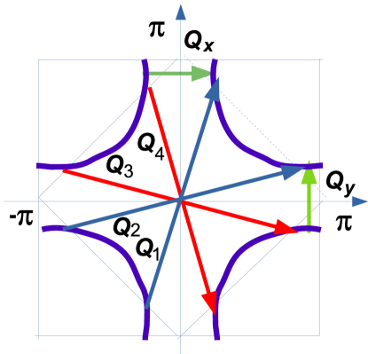
Figure 1: The Fermi surface in the Brillouin zone for a nearly half-filled square lattice model and vectors of SDW, CDW.

Consider states near the Fermi surface (FS) (see Fig.1) and use linear approximation for the quasiparticles spectrum. We write the functions $u({\bf r})$ and $v({\bf r})$ as:

$$u_{\sigma}({\bf r})=\sum_{n}\sum_{{\bf p}\in FS}[u_{{\bf p},\sigma}({\bf r})e^{i{\bf p}{\bf r}}+\sigma u_{{\bf p}-{\bf Q}_{n},\sigma}({\bf r})e^{i({\bf p}-{\bf Q}_{n}){\bf r}}],$$ (7)

$$v_{\sigma}({\bf r})=\sum_{n}\sum_{{\bf p}\in FS}[v_{{\bf p},\sigma}({\bf r})e^{i{\bf p}{\bf r}}+\sigma v_{{\bf p}-{\bf Q}_{n},\sigma}({\bf r})e^{i({\bf p}-{\bf Q}_{n}){\bf r}}],$$ (8)

where ${\bf Q}_{n}$, with $n=\{1,2\},\{3,4\}$, or ${\bf Q}_{x},{\bf Q}_{y}$ are vectors of a bidirectional SDW. Note, that both vectors ${\bf Q}_{n},\,n=\{1,2\},\{3,4\}$ from each couple in Fig. 1 $\{1,2\}$ or $\{3,4\}$ connect ${\bf p},{\bf p}-{\bf Q}$-states from the d-wave segments with the same sign (as is opposite to the case considered previously in EPL15 ). The vectors in Fig.1 are chosen to obey the following relations:

$${\bf Q}_{1,2}=(\pi,\pi)\pm(-b,b),\,{\bf Q}_{3,4}=(\pi,\pi)\pm(b,b),$$ (9)

$${\bf Q}_{1}+{\bf Q}_{2}\equiv{\bf Q}_{3}+{\bf Q}_{4}\equiv 0(\text{mod}\,2\pi),$$ (10)

$${\bf Q}_{2}\equiv-{\bf Q}_{1},\,{\bf Q}_{4}\equiv-{\bf Q}_{3},$$ (11)

$${\bf Q}_{1}+{\bf Q}_{3}\equiv 2{\bf Q}_{y},\,{\bf Q}_{1}-{\bf Q}_{3}\equiv-2{\bf Q}_{x},$$ (12)

In the general case of a doped system vectors ${\bf Q}_{n}$ are independent and we rewrite the SDW order parameter as

$$\Delta_{s}({\bf r})=\sum_{n}\Delta_{s,n}({\bf r})\exp(i{\bf Q}_{n}{\bf r})+h.c.$$

with slowly varying functions $\Delta_{s,n}({\bf r})$. Eigenvalue equations (5), (6) take the form

$\hat{H}\Psi=E\Psi$, with the Hamiltonian operator

$$\hat{H}=\left(\matrix{-i{\bf v}_{{\bf p}}\nabla_{{\bf r}}+\epsilon_{{\bf p}}-\mu&\Delta_{s,n}({\bf r})&\Delta_{-{\bf p}}&0\cr\Delta^{*}_{s,n}({\bf r})&-i{\bf v}_{{\bf p}-{\bf Q}}\nabla_{{\bf r}}+\epsilon_{{\bf p}-{\bf Q}}-\mu&0&\Delta_{-({\bf p}-{\bf Q})}\cr\Delta_{{\bf p}}^{*}&0&i{\bf v}_{{\bf p}}\nabla_{{\bf r}}-\epsilon_{{\bf p}}+\mu&\Delta_{s,n}({\bf r})\cr 0&\Delta_{{\bf p}-{\bf Q}}^{*}&\Delta^{*}_{s,n}({\bf r})&i{\bf v}_{{\bf p}-{\bf Q}}\nabla_{{\bf r}}-\epsilon_{{\bf p}-{\bf Q}}+\mu}\right),$$ (13)

where $\Psi^{T}=(u_{{\bf p}},u_{{\bf p}-{\bf Q}},v_{{\bf p}},v_{{\bf p}-{\bf Q}})=(u_{+},u_{-},v_{+},v_{-})$, $\epsilon_{{\bf p}}=-2t(\cos p_{x}+\cos p_{y})-\mu$, ${\bf v}_{{\bf p}}=2t(\sin p_{x},\sin p_{y})$.

We have linearized free particle spectrum near the Fermi surface (FS) in the Eq.(13). Note, that at zero temperature we have at the FS the identity $\epsilon({\bf p})=\epsilon({\bf p}-{\bf Q})=\mu$. For the case of $d_{x^{2}-y^{2}}$ symmetry we obtain $\Delta_{-{\bf p}}=\Delta_{{\bf p}}=\Delta_{{\bf p}-{\bf Q}}=2(\cos p_{x}-\cos p_{y})\Delta_{d}({\bf r})$, since vectors ${\bf p}$ and ${\bf p}-{\bf Q}$ are symmetric either with respect to the origin point ${\bf p}=0$, then ($-{\bf p}={\bf p}-{\bf Q}$), or with respect to the axis $p_{x}$ or $p_{y}$.(See Fig. 1).

The SDW order parameter may have $d_{x^{2}-y^{2}}$ symmetry also, then we add the index ${\bf p}$ to the SDW order parameter ($\Delta_{s}\to\Delta_{s,{\bf p}}$).

In the homogeneous case $\rho(r)=\rho,\,\Delta_{s,{\bf p}}(r)=\Delta_{s,{\bf p}},\,\Delta_{{\bf p}}(r)=\Delta_{{\bf p}}$, the eigenvalue spectrum has the form

$$E^{2}({\bf p})=\xi_{{\bf p}}^{2}+(\Delta_{{\bf p}}\pm\Delta_{s,{\bf p}})^{2},$$ (14)

where $\xi_{{\bf p}}={\bf v}_{{\bf p}_{F}}\centerdot({\bf p}-{\bf p}_{F})$, and ${\bf p}_{F}\in FS$. It follows that we have pseudogap structure of the spectrum. Moreover, we obtain the pseudogap every time when SC coexists with SDW or CDW.

In the general case a solution of system of equations (13) is unknown. But for quasi-1D structures we can use the ansatz which was applied for 1D model EPL15 ; 1d

$$v_{\pm}({\bf r})=\gamma_{\pm}u_{\mp}({\bf r}),$$

with constant $\gamma_{\pm}$. For the case

$$\Delta_{s}({\bf r})=|\Delta_{s}({\bf r})|e^{i\varphi},\,\Delta_{{\bf p}}({\bf r})=|\Delta_{{\bf p}}({\bf r})|e^{i\varphi_{s}},\,\varphi,\,\varphi_{s}=const,$$

the ansatz is satisfied at $\gamma_{+}=\pm e^{i(\varphi-\varphi_{s})},\,\gamma_{-}=\pm e^{-i(\varphi+\varphi_{s})}$, and 4x4 matrix equations (13) are reduced to 2x2 BdG type system

$$-i{\bf v}_{{\bf p}}\nabla u_{+}+\tilde{\Delta}({\bf r})u_{-}=Eu_{+}$$ (15)

$$\tilde{\Delta}^{*}({\bf r})u_{+}+i{\bf v}_{{\bf p}}\nabla u_{-}=Eu_{-}$$ (16)

with function $\tilde{\Delta}({\bf r})=(\Delta_{s}({\bf r})\pm\Delta_{{\bf p}}({\bf r}))e^{i\varphi}$. Equations (15), (16) are exact, provided that phases $\varphi$, $\varphi_{s}$ are constant or slowly varying in space functions.

The solution is the same as in 1D case 1d . The one-stripe structure is described by the solution

$$\tilde{\Delta}^{\pm}_{{\bf p}}(x)=\Delta_{{\bf p}}\tanh(\Delta_{{\bf p}}x/v_{F}\pm a/2),$$ (17)

where the dimensionless parameter $a$ is found by the minimization of the free energy. The nonzero value $a$ is reached in the region $|g_{s}-g_{sc}|\ll g_{sc}$.

In this region we have nonzero both sc and spin order parameters

$$\Delta_{s}=(\tilde{\Delta}^{+}_{p}+\tilde{\Delta}^{-}_{p})/2=\Delta_{{\bf p}}\tanh(\Delta_{{\bf p}}x)\frac{\cosh^{2}(\Delta_{p}x)}{\cosh^{2}(\Delta_{p}x)+\sinh^{2}(a/2)}$$ (18)

$$\Delta_{sc}=(\tilde{\Delta}^{+}_{p}-\tilde{\Delta}^{-}_{p})/2=\Delta_{p}\tanh(a/2)\frac{\cosh^{2}(a/2)}{\cosh^{2}(a/2)+\sinh^{2}(\Delta_{p}x)}$$ (19)

An increase of doping leads to the periodic structure (PDW + SDW) with the solution:

$$\tilde{\Delta}^{\pm}_{{\bf p}}=\Delta_{0}\tanh(\Delta_{0}x\pm a/2)\to\tilde{\Delta}\sqrt{k}\,\rm{sn}(\tilde{\Delta}x/\sqrt{k}\pm a/2,k),$$ (20)

where $\rm{sn}(\tilde{\Delta}x/\sqrt{k},k)$ is the Jakobi elliptic function with the parameter $0<k<1$ defined by the period of the structure $l=4\pi K(k)\sqrt{k}/\tilde{\Delta}$ ( $l=2/|\rho-1|$ for purely 1D model), where $K(k)$ is the complete elliptic integral of the first kind. Parameter $k$ varies from $k=1$ where ${\rm sn}(\Delta x/\sqrt{k},k)=\tanh(\Delta x)$, to $k\ll 1$ where ${\rm sn}(\Delta x/\sqrt{k},k)\sim\sin(2\pi x/l)$. The typical picture of coexisting order parameters is shown in Fig. 2, where we used values $k=0.99$ and $a=1$.

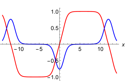
Figure 2: PDW (red) and SDW (blue) order parameters.

We see that superconductivity and antiferromagnetic ordering competes with each other: a decrease in one parameter leads to an increase in another.

II.2 Coexistence of Charge Density Wave and Superconductivity

Now, consider the case of coexistence of CDW and PDW, as observed in e.g. YBCO doped compounds Frad16 .

Eigenvalue equations differ from (5)- (6) by substitution $\sigma\Delta_{s}\to\Delta_{c}$. In the general case we rewrite the CDW order parameter as

$$\Delta_{c}({\bf r})=\sum_{n}\Delta_{c,n}({\bf r})\exp(i{\bf Q}_{n}{\bf r})+h.c.$$

with slowly varying functions $\Delta_{c,n}$. Consider the experimentally observed case of the CDW wave vector along the horizontal axis: ${\bf Q}={\bf Q}_{x}$, as shown in Fig.1 The general form of the superconducting order parameter has the form $\Delta_{{\bf p}}({\bf r})=\Delta_{{\bf p},1}({\bf r})+\Delta_{{\bf p},2}\exp i{\bf Q}_{x}{\bf r}+h.c.$ , where the second term is due to pairing of particles with nonzero momentum and describes PDW.

Instead of transformations (7) - (8) we use the same ones, but without the multiplier $\sigma$ in the second term:

$$u_{\sigma}({\bf r})=\sum_{{\bf p}\in FS,p_{x}>0}[u_{{\bf p},\sigma}e^{i{\bf p}{\bf r}}+u_{{\bf p}-{\bf Q},\sigma}({\bf r})e^{i({\bf p}-{\bf Q}){\bf r}}],$$ (21)

We obtain instead of (13) the eigenvalue equations: $\hat{H}\Psi=E\Psi$, with the Hamiltonian operator

$$\hat{H}=\left(\matrix{-iV_{{\bf p}}\nabla_{{\bf r}}+\epsilon_{{\bf p}}-\mu&\Delta_{c}({\bf r})&\Delta_{-{\bf p},1}&\Delta_{-{\bf p},2}\cr\Delta_{c}^{*}({\bf r})&-iV_{{\bf p}-{\bf Q}}\nabla_{{\bf r}}+\epsilon_{{\bf p}-{\bf Q}}-\mu&\Delta_{-({\bf p}-{\bf Q}),2}&\Delta_{-({\bf p}-{\bf Q}),1}\cr\Delta_{{\bf p},1}^{*}&\Delta_{{\bf p},2}^{*}&iV_{{\bf p}}\nabla_{{\bf r}}-\epsilon_{{\bf p}}+\mu&\Delta_{c}({\bf r})\cr\Delta_{{\bf p}-{\bf Q},1}^{*}&\Delta_{{\bf p}-{\bf Q},1}^{*}&\Delta_{c}^{*}({\bf r})&iV_{{\bf p}-{\bf Q}}\nabla_{{\bf r}}-\epsilon_{{\bf p}-{\bf Q}}+\mu}\right).$$ (22)

Note, that for the case $\Delta_{{\bf p},2}=0$ these equations coincide with those obtained for the case of a spin density wave (13).

Equations can be simplified also for the case of pure PDW ($\Delta_{p,1}=0$). Similar to the previous section, we obtain instead of (15), (16) the following effective 2x2 equations

$$-i{\bf v}_{{\bf p}}\nabla u_{+}+{\Delta_{c}}({\bf r})u_{-}=(E\mp|\Delta_{p}|)u_{+}$$ (23)

$${\Delta_{c}}^{*}({\bf r})u_{+}+i{\bf v}_{{\bf p}}\nabla u_{-}=(E\mp|\Delta_{p}|)u_{-},$$ (24)

where we used the symmetry of the order parameter: $\Delta_{{\bf p}-{\bf Q}_{x}}=\Delta_{{\bf p}}$, since ${\bf p}=\{p_{x},p_{y}\}$, ${\bf p}-{\bf Q}_{x}=\{-p_{x},p_{y}\}$. Note, that the homogeneous solution has the two branch excitation spectrum

$$E({\bf p})=|\sqrt{\xi_{p}^{2}+|\Delta_{c}|^{2}}\pm|\Delta_{{\bf p}}||$$ (25)

(For the case of $d$-symmetry of the CDW order parameter we should substitute $\Delta_{c}\to\Delta_{c,{\bf p}}=(\cos p_{x}-\cos p_{y})\Delta_{c}$.)

This solution describes coexisting CDW and PDW, both with the same wave vector along the horizontal axis $\hat{x}$ and having the same period $=2\pi/Q_{x}$:

$\rho(x)-\bar{\rho}\sim\Delta_{c}\cos(Q_{x}x)$, $\Delta(x)-\bar{\Delta}\sim\Delta_{p}\cos(Q_{x}x)$,

as is observed e.g. in the field induced PDW state in the halo surrounding the vortex core in Bi₂Sr₂CaCu2O₈ pdwH18 .

Based on a simple 2D t-U-V Hubbard model on a square lattice we presented different solutions, describing periodic charge-spin and superconducting pair density structures. Charge/spin and superconducting states competes with each other: a decrease in one parameter induces an increase in another. This is a possible reason for the appearance of pair density waves: oscillations of SDW/CDW generate oscillations of the superconducting order parameter. On the other hand, a decrease in the superconducting order parameter in a vortex region results in an appearance of SDW/CDW oscillations. The existence of CDW/SDW essentially influences the band structure of superconductors.

References

• (1) B. Lake, H.M. Rùnnow, N. B. Christensenk, G. Aeppli et.al.,Nature 415, 299 (2002).
• (2) Erez Berg et al 2009 New J. Phys. 11, 115004
• (3) P. Fulde and R. A. Ferrell, Physical Review 135, A550 (1964).
• (4) A. Larkin and I. Ovchinnikov, Soviet Physics-JETP 20, 762 (1965).
• (5) Yuxuan Wang, Stephen D. Edkins, Mohammad H. Hamidian, J. C. Seamus Davis, Eduardo Fradkin, and Steven A. Kivelson, Phys. Rev. B 97, 174510 (2018).
• (6) Zhehao Dai, Ya-Hui Zhang, T. Senthil, and Patrick A. Lee, Phys. Rev. B 97, 174511 (2018).
• (7) A. Himeda, T. Kato, and M. Ogata, Phys. Rev. Lett. 88, 117001 (2002).
• (8) S. I. Matveenko and S. I. Mukhin, EPL, 109, 57007 (2015).
• (9) S.I. Mukhin, Phys. Rev. B 62, 4332 (2000)
• (10) S.I. Matveenko, and S.I. Mukhin, Phys. Rev. Lett. 84, 6066 (2000).
• (11) S. I. Matveenko, JETP Lett. 78, 384 (2003).
• (12) Jinsheng Wen, Qing Jie, Qiang Li et al,PRB 85, 134513 (2012).
• (13) Eduardo Fradkin, Steven A. Kivelson, John M. Tranquada, Rev. Mod. Phys. 87, 457 (2015).
• (14) V. Khanna, R. Mankowsky, M. Petrich, H. Bromberger, S. A. Cavill, E. Möhr-Vorobeva, D. Nicoletti, Y. Laplace, G. D. Gu, J. P. Hill, M. Först, A. Cavalleri, and S. S. Dhesi, Phys. Rev. B 93, 224522 (2016).
• (15) S. D. Edkins, A. Kostin, K. Fujita, A. P. Mackenzie, H. Eisaki, S. Uchida, Subir Sachdev, M. J. Lawler, E. -A. Kim, J. C. Seamus Davis, and M. H. Hamidian, Science 364, 976 (2019).
• (16) E.M. Forgan, E. Blackburn, A.T. Holmes,w, A. K. R. Briffa, J. Chang, L. Bouchenoire, S.D. Brown3, Ruixing Liang, D. Bonn, W.N. Hardy, N.B. Christensen, M.v. Zimmermann, M. Huc̈ker and S.M. Hayden NATURE COMMUNICATIONS — 6:10064 — DOI: 10.1038/ncomms10064
• (17) Yuxuan Wang, Daniel F. Agterberg, and Andrey Chubukov, Phys. Rev. Lett. 114, 197001 (2015); Phys. Rev. B 91, 115103 (2015)
• (18) Andrea Allais, Johannes Bauer, and Subir Sachdev, Phys. Rev. B 90, 155114 (2014).
• (19) J. Tranquada, Nature (London) 375, 561 (1995).
• (20) F. Loder et al., New J. Phys. 13, 113037 (2011).
• (21) Mats Barkman, Albert Samoilenka, and Egor Babaev, Phys. Rev. Lett. 122, 165302 (2019).