A linearized framework and a new benchmark for model selection for fine-tuning

Abstract

Fine-tuning from a collection of models pre-trained on different domains (a “model zoo”) is emerging as a technique to improve test accuracy in the low-data regime. However, model selection, i.e. how to pre-select the right model to fine-tune from a model zoo without performing any training, remains an open topic. We use a linearized framework to approximate fine-tuning, and introduce two new baselines for model selection – Label-Gradient and Label-Feature Correlation. Since all model selection algorithms in the literature have been tested on different use-cases and never compared directly, we introduce a new comprehensive benchmark for model selection comprising of: $i)$ A model zoo of single and multi-domain models, and $ii)$ Many target tasks. Our benchmark highlights accuracy gain with model zoo compared to fine-tuning Imagenet models. We show our model selection baseline can select optimal models to fine-tune in few selections and has the highest ranking correlation to fine-tuning accuracy compared to existing algorithms.

1 Introduction

(a) Model zoo vs. different architectures. Fine-tuning using our model zoo is better (i.e. lower test error) than fine-tuning using different architectures with Random or Imagenet pre-trained initialization. We use fine-tuning hyper-parameters of sec:finetune with $\eta=.005$.

(b) Model zoo vs. HPO. of Imagenet expert Fine-tuning using our model zoo is better than fine-tuning with hyper-parameter optimization (HPO) on Imagenet pre-trained Resnet-101 model. We use fine-tuning hyper-parameters of sec:finetune and perform HPO with $\eta=.01,.005,0.001$.

Figure 1: Fine-tuning using our model zoo can obtain lower test error compared to: $(a)$ using different architectures and $(b)$ hyper-parameter optimization (HPO) of Imagenet expert. The standard fine-tuning approach entails picking a network architecture pre-trained on Imagenet to fine-tune and performing hyper-parameter optimization (HPO) during fine-tuning. We outperform this strategy by fine-tuning using our model zoo described in sec:model_zoo. We plot test error as a function of the number of per-class samples (i.e. shots) in the dataset. In $(a)$, we compare fine-tuning with our single-domain experts in the model zoo to using different architectures (AlexNet, ResNet-18, ResNet-101, Wide ResNet-101) for fine-tuning. In $(b)$, we show fine-tuning with our model zoo obtains lower error than performing HPO on Imagenet pre-trained Resnet-101 [19] during fine-tuning. Model zoo lowers the test error, especially in the low-data regime (5, 10, 20-shot per class samples of target task). Since we compare to Imagenet fine-tuning, we exclude Imagenet experts from our model zoo for the above plots.

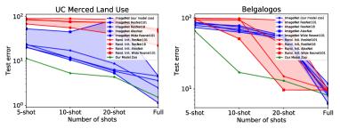
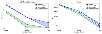
A “model zoo” is a collection of pre-trained models, obtained by training different architectures on many datasets covering a variety of tasks and domains. For instance, the zoo could comprise models (or experts) trained to classify, say, trees, birds, fashion items, aerial images, etc. The typical use of a model zoo is to provide a good initialization which can then be fine-tuned for a new target task, for which we have few training data. This strategy is an alternative to the more common practice of starting from a model trained on a large dataset, say Imagenet [13], and is aimed at providing better domain coverage and a stronger inductive bias. Despite the growing usage of model zoos [10, 26, 31, 48] there is little in the way of analysis, both theoretical and empirical, to illuminate which approach is preferable under what conditions. In fig:efficiency-curve, we show that fine-tuning with a model zoo is indeed better, especially when training data is limited. fig:efficiency-curve also shows that using a model zoo, we can outperform hyper-parameter optimization performed during fine-tuning of the Imagenet pre-trained model.

Fine-tuning with a model zoo can be done by brute-force fine-tuning of each model in the zoo, or more efficiently by using “model selection” to select the closest model (or best initialization) from which to fine-tune. The goal of model selection therefore is to find the best pre-trained model to fine-tune on the target task, without performing the actual fine-tuning. So, we seek an approximation to the fine-tuning process. In our work, we develop an analytical framework to characterize the fine-tuning process using a linearization of the model around the point of pre-training [35], drawing inspiration from the work on the Neural Tangent Kernel (NTK) [24, 29]. Our analysis of generalization bounds and training speed using linearized fine-tuning naturally suggests two criterion to select the best model to fine-tune from, which we call Label-Gradient Correlation (LGC) and Label-Feature Correlation (LFC). Given its simplicity, we consider our criteria as baselines, rather than full-fledged methods for model selection, and compare the state-of-the-art in model selection – e.g. RSA [15], LEEP [37], Domain Similarity [10], Feature Metrics [49] – against it.

Model selection being a relatively recent endeavor, there is currently no standard dataset or a common benchmark to perform such a comparison. For example, LEEP [37] performs its model selection experiments on transfer (or fine-tuning) from Imagenet pre-trained model to $200$ randomly sampled tasks of CIFAR-100 [28] image classification, RSA [15] uses the Taskonomy dataset [55] to evaluate its prediction of task transfer (or model selection) performance. Due to these different experimental setups, the state-of-the-art in model selection is unclear. Therefore, in sec:experiments we build a new benchmark comprising a large model zoo and many target tasks. For our model zoo, we use $8$ large image classification datasets (from different domains) to train single-domain and multi-domain experts. We use various image classification datasets as target tasks and study fine-tuning (sec:finetune) and model selection (sec:model_selection) using our model zoo. To the best of our knowledge ours is the first large-scale benchmark for model selection.

By performing fine-tuning and model selection on our benchmark, we discover the following:

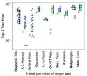
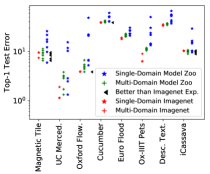
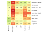
1. We show (fig:efficiency-curve) that fine-tuning models in the model zoo can outperform the standard method of fine-tuning with Imagenet pre-trained architectures and HPO. We obtain better fine-tuning than Imagenet expert with, both model zoo of single-domain experts (fig:finetune_full) and multi-domain experts (fig:finetune_universal). While in the high-data regime using a model zoo leads to modest gains, it sensibly improves accuracy in the low-data regime.

2. For any given target task, we show that only a small subset of the models in the zoo lead to accuracy gain (fig:finetune_full). In such a scenario, brute-force fine-tuning all models to find the few that improve accuracy is wasteful. Fine-tuning with all our single-domain experts in the model zoo is $40\times$ more compute intensive than fine-tuning an Imagenet Resnet-101 expert in tab:runtime.

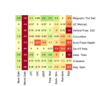
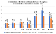
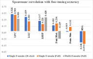
3. Our LGC model selection, and particularly its approximation LFC, can find the best models from which to fine-tune without requiring an expensive brute-force search (tab:runtime). With only $3$ selections, we can select models that show gain over Imagenet expert (fig:model_zoo_selection_top3). Compared to Domain Similarity [11], RSA [15] and Feature Metrics [49], our LFC score can select the best model to fine-tune in fewer selections, and it shows the highest ranking correlation to the fine-tuning test accuracy (fig:trials) among all model selection methods.

2 Related work

Fine-tuning. The exact role of pre-training and fine-tuning in deep learning is still debated. He et al. [20] show that, for object detection, the accuracy of a pre-trained model can be matched by simply training a network from scratch but for longer. However, they notice that the pre-trained model is more robust to different hyper-parameters and outperforms training from scratch in the low-data regime. On the other hand, in fine-grained visual classification, Li et al. [31] show that even after hyper-parameter optimization (HPO) and with longer training, models pre-trained on similar tasks can significantly outperform both Imagenet pre-training and training from scratch. Achille et al. [1], Cui et al. [11] study task similarity and also report improvement in performance by using the right pre-training. Zoph et al. [58] show that while pre-training is useful in low-data regime, self-training outperforms pre-training in high-data regime. Most of the above work,  [2, 11, 31] draws inferences of transfer learning by using Imagenet [13] or iNaturalist [21] experts. We build a model zoo with many more single domain and multi-domain experts (sec:model_zoo), and use various target tasks (sec:finetune) to empirically study transfer learning in different data regimes.

Model Selection. Empirical evidence [1, 31, 54] and theory [2] suggests that effectiveness of fine-tuning relates to a notion of distance between tasks. Taskonomy [54] defines a distance between learning tasks a-posteriori, that is, by looking at the fine-tuning accuracy during transfer learning. However, for predicting the best pre-training without performing fine-tuning, an a-priori approach is best. Achille et al. [1, 2] introduce a fixed-dimensional “task embedding” to encode distance between tasks. Cui et al. [11] propose a Domain Similarity measure, which entails using the Earth Mover Distance (EMD) between source and target features. LEEP [37, 46] looks at the conditional cross-entropy between the output of the pre-trained model and the target labels. RSA [15] compares representation dissimilarity matrices of features from pre-trained model and a small network trained on target task for model selection. As opposed to using the ad-hoc measure of task similarity, we rely on a linearization approximation to the fine-tuning to derive our model selection methods (sec:approach).

Linearization and NTK. To analyse fine-tuning from pre-trained weights, we use a simple but effective framework inspired by the Neural Tangent Kernel (NTK) formalism [24]: We approximate the fine-tuning dynamics by looking at a linearization of the source model around the pre-trained weights $w_{0}$ (sec:linearization). This approximation has been suggested by [35], who also notes that while there may be doubts on whether an NTK-like approximation holds for real randomly-initialized network [16], it is more likely to hold in the case of fine-tuning, since the fine-tuned weights tend to remain close to the pre-trained weights.

Few-shot. Interestingly, while pre-training has a higher impact in the few-shot regime, there is only a handful of papers that experiment with it [14, 18, 47]. This could be due to over-fitting of the current literature on standard benchmarks that have a restricted scope. We hope that our proposed benchmark (sec:experiments) may foster further research.

3 Approach

Notation. We have a model zoo, $\mathcal{F}$, of $n$ pre-trained models or experts: $\mathcal{F}=\{f^{1},f^{2},\cdots f^{n}\}$. Our aim is to classify a target dataset, $\mathcal{D}=\{(x_{i},y_{i})\}_{i=1}^{N}$, by fine-tuning models in the model zoo. Here, $x_{i}\in{\cal X}$, is the $i^{th}$ input image and $y_{i}\in{\cal Y}$, is the corresponding class label. For a network $f\in\mathcal{F}$ with weights $w$, we denote the output of the network with $f_{w}(x)$. $w_{0}$ denotes the initialization (or pre-trained weights) of models in the model zoo. The goal of model selection is to predict a score $S(f_{w_{0}},\mathcal{D})$ that measures the fine-tuning accuracy on the test set $\mathcal{D}^{\text{test}}$, when $\mathcal{D}$ is used to fine-tune the model $f_{w_{0}}$. Note, $S$ does not have to exactly measure the fine-tuning accuracy, it needs to only predict a score that correlates to the ranking by fine-tuning accuracy. The model selection score for every pre-trained model, $S(f^{k},\mathcal{D})$ for $k\in\{1,2,\cdots,n\}$, can then be used as proxy to rank and select top-$k$ models by their fine-tuning accuracy. Since the score $S$ needs to estimate (a proxy for) fine-tuning accuracy without performing any fine-tuning, in sec:linearization we construct a linearization approximation to fine-tuning and present several results that allow us to derive our Label-Gradient Correlation ($S_{LG}$) and Label-Feature Correlation ($S_{LF}$) (sec:label-correlation) scores for model selection from it. In fig:trials (b), we show our scores have higher ranking correlation to fine-tuning accuracy than existing work.

3.1 Linearized framework to analyse fine-tuning

Given an initialization $w_{0}$, the weights of the pre-trained model, we can define the linearized model:

$$f^{\text{lin}}_{w}(x):=f_{w_{0}}(x)+\nabla_{w}f_{w_{0}}(x)|_{w=w_{0}}(w-w_{0}),$$

which approximates the output of the real model for $w$ close to $w_{0}$. Mu et al. [35] observe that, while in general not accurate, a linear approximation can correctly describe the model throughout fine-tuning since the weights $w$ tend to remain close to the initial value $w_{0}$. Under this linear approximation [29] shows the following proposition,

Proposition 1

Let $\mathcal{D}=\{(x_{i},y_{i})\}_{i=1}^{N}$ be the target dataset. Assume the task is a binary classification problem with labels $y_{i}=\pm 1$, using the $L_{2}$ loss $L_{\mathcal{D}}(w)=\sum_{i=1}^{N}(y_{i}-f_{w}(x_{i}))^{2}$. Let $w_{t}$ denote the weights at time $t$ during training. Then, the loss function evolve as:

$$L_{t} =(\mathcal{Y}-f_{w_{0}}(\mathcal{X}))^{T}e^{-2\eta\Theta t}(\mathcal{Y}-f_{w_{0}}(\mathcal{X}))$$ (1)

where $f_{w_{0}}(\mathcal{X})$ denotes the vector containing the output of the network on all the images in the dataset, $\mathcal{Y}$ denotes the vectors of all training labels, and we defined the Neural Tangent Kernel (NTK) matrix:

$$\Theta:=\nabla_{w}f_{w}(\mathcal{X})\nabla_{w}f_{w}(\mathcal{X})^{T}$$ (2)

which is the $N\times N$ Gram matrix of all the per-sample gradients.

From Prop. 1, the behavior of the network during fine-tuning is fully characterized by the kernel matrix $\Theta$, which depends on the pre-trained model $f_{w_{0}}$, the data $\mathcal{X}$ and the task labels $\mathcal{Y}$. We then expect to be able to select the best model by looking at these quantities. To show how we can do this, we now derive several results connecting $\Theta$ and $\mathcal{Y}$ to the quantities of relevance for model selection below, i.e. Training time and Generalization on the target task.

Training time. In  [56], it is shown that the loss $L_{t}$ of the linearized model evolves with training over time $t$ as

$$L_{t}=\|\delta\mathcal{Y}\|^{2}-t\delta\mathcal{Y}^{T}\Theta\delta\mathcal{Y}+O(t^{2}).$$ (3)

where we have defined $\delta\mathcal{Y}=\mathcal{Y}-f_{w_{0}}(\mathcal{X})$ to be the initial projection residual. Eq. (3) suggests using the quadratic term $\delta\mathcal{Y}^{T}\Theta\delta\mathcal{Y}$ as a simple estimate of the training speed.

Generalization. The most important criterion for model selection is generalization performance. Unfortunately, we cannot have any close form characterization of generalization error, which depends on test data we do not have. However, in [3] the following bound on the test error is suggested:

$$L_{\text{test}}^{2}\leq\frac{1}{n}\mathcal{Y}^{T}\Theta^{-1}\mathcal{Y}=\frac{1}{n}\sum_{k}\frac{1}{\lambda_{k}}(\mathcal{Y}\cdot v_{k})^{2}.$$ (4)

We see that if $\mathcal{Y}$ correlates more with the first principal components of variability of the per-sample gradients (so that $\mathcal{Y}\cdot v_{k}$ is larger), then we expect better generalization.

Arora et al. [3] prove that this bound holds with high-probability for a wide-enough randomly initialized 3-layer network. In practice, however, this generalization bound may be vacuous as hypotheses are not satisfied (the network is deeper, and the initialization is not Gaussian). For this reason, rather than using the above quantity as a real bound, we refer to it as an empirical “generalization score”.

Note eq. 3 and eq. 4 contain the similar terms $\delta\mathcal{Y}^{T}\Theta\delta\mathcal{Y}$ and $\delta\mathcal{Y}^{T}\Theta^{-1}\delta\mathcal{Y}$. By diagonalizing $\Theta$ and applying Jensen’s inequality we have the following relation between the two:

$$\Big{(}\frac{\delta\mathcal{Y}^{T}\Theta\delta\mathcal{Y}}{\|\delta\mathcal{Y}\|^{2}}\Big{)}^{-1}\leq\frac{\delta\mathcal{Y}^{T}\Theta^{-1}\delta\mathcal{Y}}{\|\delta\mathcal{Y}\|^{2}}.$$ (5)

Hence, good “generalization score” $\delta\mathcal{Y}^{T}\Theta^{-1}\delta\mathcal{Y}$ implies faster initial fine-tuning, that is, larger $\delta\mathcal{Y}^{T}\Theta\delta\mathcal{Y}$. In general we expect the two quantities to be correlated. Hence, selecting the fastest model to train or the one that generalizes better are correlated objectives. $\mathcal{Y}^{T}\Theta\mathcal{Y}$ is an approximation to $\delta\mathcal{Y}^{T}\Theta\delta\mathcal{Y}$ that uses task labels $\mathcal{Y}$ and kernel $\Theta$, and we use it to derive our model selection scores in sec:label-correlation. Large value of $\mathcal{Y}^{T}\Theta\mathcal{Y}$ implies better generalization and faster training and it is desirable for a model when fine-tuning.

Should model selection use gradients or features? Our analysis is in terms of the matrix $\Theta$ which depends on the network’s gradients (2), not on its features. In sec:proof, we show that it suffices to use features (i.e. network activations) in (2) as an approximation to the NTK matrix. Let $[f(x_{i})]_{l}$ denote the feature vector (or activation) extracted from layer $l$ of pre-trained network $f$ after forward pass on image, i.e. after $f(x_{i})$. In analogy with the gradient similarity matrix $\Theta$ of (2), we define the feature similarity matrix $\Theta_{F}$ (which approximates $\Theta$) as follows

$$\Theta_{F}:=[f_{w}(\mathcal{X})]_{l}[f_{w}(\mathcal{X})]_{l}^{T}.$$ (6)

3.2 Label-Feature and Label-Gradient correlation

We now introduce our two scores for model selection, Label-Gradient correlation and Label-Feature correlation.

Label-Gradient Correlation. From sec:linearization we know that the following score,

$$S_{\text{LG}}(f_{w_{0}},\mathcal{D})=\mathcal{Y}^{T}\Theta\mathcal{Y}=\Theta\cdot\mathcal{Y}\mathcal{Y}^{T}$$ (7)

which we call Label-Gradient Correlation (LGC), can be used to estimate both the convergence time (eq. 3) and the generalization ability of a model. Here, “$\cdot$” denotes the dot-product of the matrices (i.e. the sum of Hadamard product of two matrices). $\mathcal{Y}\mathcal{Y}^{T}$ is an $N\times N$ matrix such that $(\mathcal{Y}\mathcal{Y}^{T})_{i,j}=1$ if $x_{i}$ and $x_{j}$ have the same label and $-1$ otherwise. For this reason, we call $\mathcal{Y}\mathcal{Y}^{T}$ the label similarity matrix. On the other hand, $\Theta_{ij}=\nabla_{w}f_{w_{0}}(x_{i})\cdot\nabla_{w}f{w_{0}}(x_{j})$ is the pair-wise similarity matrix of the gradients. Hence, eq. 7 can be interpreted as giving high LG score (i.e., the model is good for the task) if the gradients are similar whenever the labels are also similar, and are different otherwise.

Label-Feature Correlation. Instead of $\Theta$, we can use the approximation $\Theta_{F}$ from (6) and define our Label-Feature Correlation (LFC) score as:

$$S_{\text{LF}}=\mathcal{Y}^{T}\Theta_{F}\mathcal{Y}=\Theta_{F}\cdot\mathcal{Y}\mathcal{Y}^{T}.$$

Similarly to the LGC score, this score is higher if samples with the same labels have similar features extracted from the pre-trained network.

3.3 Implementation

Notice that the scores $S_{\text{LG}}$ and $S_{\text{LF}}$ are not normalized. Different pre-training could lead to very different scores if the gradients or the features have a different norm. Also, $\mathcal{Y}\mathcal{Y}^{T}$ used in our scores is specific to binary classification. In practice, we address this as follows: For a multi-class classification problem, let $K_{\mathcal{Y}}$ be the $N\times N$-matrix with $(K_{\mathcal{Y}})_{i,j}=1$ if $x_{i}$ and $x_{j}$ have the same label, and $-1$ otherwise. Let $\mu_{K}$ denote the mean of the entries of $K_{\mathcal{Y}}$, and $\mu_{\Theta}$ the mean of $\Theta$. We define the normalized LGC score as:

$$S_{\text{LG}}=\frac{(\Theta-\mu_{\Theta})\cdot(K_{\mathcal{Y}}-\mu_{K})}{\|\Theta-\mu_{\Theta}\|_{2}\|K_{\mathcal{Y}}-\mu_{K}\|_{2}},$$ (8)

We normalize LFC similar to LGC in (8). This can also be interpreted as the Pearson’s Correlation coefficient between the entries of $\Theta$ (or $\Theta_{F}$) and the entries of $K_{\mathcal{Y}}$, justifying the name label-gradient (or label-feature) correlation.

Which features and gradients to use? For LFC, we extract features from the layer before the fully-connected classification layer (for both Resnet-101 [19] and Densenet-169 [22] models in our model zoo of sec:model_zoo). We use these features to construct our $\Theta_{F}$ and compute the normalized LFC. For LGC, following [35], we use gradients corresponding to the last convolutional layer in the pre-trained network. For a large gradient vector, to perform fast computation of LGC, we take a random projection to $10K$ dimensions and compute the normalized LGC score. This results in a trade-off between accuracy and computation for LGC.

Sampling of target task. Model selection is supposed to be an inexpensive pre-processing step before actual fine-tuning. To reduce its computation, following previous work of RSA [15], we sample the training set of target dataset ${\cal D}$ and pick at most $25$ images per class to compute our model selection scores. Note, test set is hidden from model selection. Our results show, this still allows us to select models that obtain accuracy gain over Imagenet expert (fig:model_zoo_selection_top3), and we need few selections ($<7$ for model zoo size $30$) to select the optimal models (fig:trials) to fine-tune. We include additional implementation details of our model selection methods and other baselines: RSA [15], Domain Similarity [11], LEEP [37], Feature Metrics [49] in sec:model_selection_impl.

	Pre-train	RESISC-45 [7]	Food-101 [6]	Logo 2k [50]	G. Landmark [39]	iNaturalist 2019 [21]	iMaterialist [33]	ImageNet [13]	Places-365 [57]
Densenet-169	$\times$	93.61	82.38	64.58	82.28	71.34	66.59	76.40	55.47
	$\checkmark$	96.34	87.82	76.78	84.89	73.65	67.57	-	55.58
Resnet-101	$\times$	87.14	79.20	62.03	78.48	70.32	67.95	77.54	55.83
	$\checkmark$	96.53	87.95	78.52	85.64	74.37	68.58	-	56.08
Reported Acc.	-	86.02 [8]	86.99 [30]	67.65 [51]	-	75.40 [40]	-	77.37[43]	54.74 [57]

Table 1: Model zoo of single-domain experts. We train $30$ models, Resnet-101 and Densenet-169, on $8$ source datasets and measure the top-1 test accuracy. We train our models starting with ($\checkmark$) and without ($\times$) Imagenet pre-training. For all datasets we have higher test accuracy with Resnet-101 ($\checkmark$) than what is reported in the literature (last row), except for iNaturalist [21] by -1.03%. We order datasets from left to right by increasing dataset size, Nwpu-resisc45 [7] has $25K$ training images while Places-365 [57] has $1.8M$. We chose datasets that are publicly available and cover different domains.

Dataset	Single Domain	Shared	Multi-BN	Adapter
Nwpu-resisc45 [7]	96.53	73.73	96.46	95.24
Food-101 [6]	87.95	48.12	87.92	86.35
Logo 2k [50]	78.52	24.39	79.06	70.13
Goog. Land [39]	85.64	65.1	81.89	76.83
iNatural. [21]	74.37	37.6	65.2	63.04
iMaterial. [33]	68.58	42.15	63.27	57.5
Imagenet [13]	77.54	52.51	69.03	58.9
Places-365 [57]	56.08	41.58	51.21	47.51

Table 2: Multi-domain expert. The top-1 test accuracy of multi-domain model – Multi-BN, Adapter – is comparable to single domain expert for small datasets (Nwpu-Resisc45, Food-101, Logo 2k), while the accuracy is lower on other large datasets. Multi-BN performs better than Shared, Adapter on all datasets and we use this as our multi-domain expert for fine-tuning and model selection.

4 Experiments

Having established the problem of model selection for fine-tuning (sec:approach), we now put our techniques to test. sec:model_zoo describes our construction of model zoos with single-domain and multi-domain experts. In sec:finetune, we then verify the advantage of fine-tuning using our model zoo with various target tasks. In sec:model_selection, we compare our LFC, LGC model selection (sec:label-correlation) to previous work, and show that our method can select the optimal models to fine-tune from our model zoo (without performing the actual fine-tuning).

4.1 Model Zoo

We evaluate model selection and fine-tuning with both, a model zoo of single-domain experts (i.e. models trained on single dataset) and a model zoo of multi-domain experts described below.

Source Datasets. tab:source_dataset and tab:suppl_datasets lists the source datasets, i.e. the datasets used for training our model zoo. We include publicly available large source datasets (from $25K$ to $1.8M$ training images) from different domains, e.g. Nwpu-resisc45 [7] consists of aerial imagery, Food-101 [6] and iNaturalist 2019 [21] consist of food, plant images, Places-365 [57] and Google Landmark v2 [39] contain scene images. This allows us to maximize the coverage of our model zoo to different domains and enables more effective transfer when fine-tuning on different target tasks.

Model zoo of single-domain experts. We build a model zoo of a total of $30$ models (Resnet-101 [19] and Densenet-169 [22]) trained on $8$ large image classification datasets (i.e. source datasets). Since each model is trained on a single classification dataset (i.e. domain), we refer to these models as single-domain experts. This results in a model zoo, $\mathcal{F}=\{f^{k}\}_{k=1}^{30}$, to evaluate our model selection.

On each source dataset of tab:source_dataset, we train Resnet-101 and Densenet-169 models for 90 epochs, with the following hyper-parameters: initial learning rate of 0.1, with decay by $0.1\times$ every 30 epochs, SGD with momentum of $.9$, weight decay of $10^{-4}$ and a batch size 512. We use the training script from PyTorch [42] library and ensure that our models are well-trained.

In tab:source_dataset, we show slightly higher top-1 test accuracy for our models trained on Imagenet [13] when compared to the PyTorch [42] model zoo. Our Resnet-101 model trained on Imagenet has $+.17\%$ top-1 test accuracy and our Densenet-169 model has $+.4\%$ top-1 test accuracy vs. PyTorch. On source datasets other than Imagenet, we train our models with ($\checkmark$) and without ($\times$) Imagenet pre-training. This allows us to study the effect of pre-training on a larger dataset when we fine-tune and perform model selection. Note that our Resnet-101 models with ($\checkmark$) Imagenet pre-training have higher accuracy compared to that reported in the literature for all source datasets, except iNaturalist [21] by $-1.03\%$.

Figure 2: Fine-tuning with model zoo of single-domain experts. We plot top-1 test error (vertical axis) for fine-tuning with different single domain models in our model zoo. For every target task (on horizontal axis), we have $4$ columns of markers from left to right: $1)$ Imagenet experts in red, $2)$ Densenet-169 experts with pre-train ($\checkmark$) and without pre-train ($\times$), $3)$ Resnet-101 experts with pre-train ($\checkmark$) and without pre-train ($\times$), $4)$ We use “black $\leftarrow$” to highlight models that perform better than imagenet expert (i.e. lower error than first column of Imagenet expert per task). Our observations are the following: $i)$ For full target task, we observe better accuracy than Imagenet expert for Magnetic Tile Defects, UC Merced Land Use and iCassava (see black $\leftarrow$). For 20 and 5-shot per class sampling of target task, with the model zoo we outperform Imagenet expert on more datasets, see Oxford Flowers 102, European Flood Depth, Belga Logos and Cub200. Our empirical result, on the importance of different pre-trainings of our model zoo experts when training data is limited, adds to the growing body of similar results in existing literature [20, 31, 58], and $ii)$ The accuracy gain over Imagenet expert is only obtained for fine-tuning with select few models for a given target task, e.g. only one expert for UC Merced Land Use target task in Full, 20-shot setting above. Therefore, brute-force fine-tuning with model zoo leads to wasteful computation. Model selection (sec:approach) picks the best models to fine-tune and avoids brute-force fine-tuning. Figure is best viewed in high-resolution.

Figure 3: Fine-tuning with the multi-domain expert for the full target task. We use the same notation as fig:finetune_full. For every target task (horizontal axis), we have $4$ columns corresponding to fine-tuning different models from left to right: $1)$ Imagenet single and multi-domain expert in red, $2)$ Fine-tuning with different domains of multi-domain expert in green and $3)$ Single-domain Resnet-101 experts in blue, $4)$ We highlight multi-domain experts that obtain lower error than Imagenet single domain with black $\leftarrow$. Note, since our multi-domain expert is Resnet-101 based, we only use all our Resnet-101 experts for for fair comparison. Our observations are: $i)$ We see gains over Imagenet expert (both single and multi-domain) by fine-tuning some (not all) domains of the multi-domain expert, for Magentic Tile Defects, Oxford Flowers 102, Cucumber and iCassava target tasks. Therefore, it is important to pick the correct domain from the multi-domain expert for fine-tuning. $ii)$ We observe the variance in error is smaller for fine-tuning with different domains of multi-domain experts, possibly due to shared parameters across domains, $iii)$ Finally in some cases, e.g. Oxford Flowers 102 and iCassava, our multi-domain experts outperform both, all single domain and Imagenet experts. Figure is best viewed in high-resolution.

Model zoo of multi-domain expert. We also train a Resnet-101 based multi-dataset (or multi-domain) [45] model on the combination of all the $8$ source datasets. Our multi-domain Resnet-101 expert, $f_{w_{s},\{w_{d}\}_{d=1}^{D}}$, uses shared weights (or layers), i.e. $w_{s}$, across different domains (or datasets), and in addition it has some domain-specific parameters, i.e. $\{w_{d}\}_{d=1}^{D}$, for each domain. We have 8 source datasets or domains, so $D=8$ in our benchmark. Note, for fine-tuning we can choose any one of the $D$ domain-specific parameters to fine-tune. For a given multi-domain expert, this results in a model zoo of $D$ models (one per domain) that we can fine-tune, $\mathcal{F}=\{f_{w_{s},w_{1}},f_{w_{s},w_{2}},\cdots,f_{w_{s},w_{D}}\}$.

We experiment with a few different variants of domain-specific parameters – $i)$ Shared: The domain-specific parameters are also shared, therefore we simply train a Resnet-101 on all datasets, $ii)$ Multi-BN: We replace each batch norm in Resnet-101 architecture with a domain-specific batch norm. Note, for a batch norm layer we replace running means, scale and bias parameters, $iii)$ Adapter: We use the domain-specific parallel residual adapters [45] within the Resnet-101 architecture. Our training hyper-parameters for the multi-domain expert are the same as our single-domain expert. The only change is that for every epoch we sample at most $100K$ training images (with replacement if $100K$ exceeds dataset size) from each dataset to balance training between different datasets and to keep the training time tractable. As we show in tab:multi_domain, Multi-BN model outperforms other multi-domain models and we use it in our subsequent fine-tuning (sec:finetune) and model selection (sec:model_selection) experiments.

(a) Full Dataset

(b) 20-Shot per class

Figure 4: Model selection among single-domain experts. The heatmap shows the accuracy gain over Resnet-101 Imagenet expert obtained by fine-tuning the top-$3$ selected models for different model selection methods (column) on our target tasks (row). Higher values of gain are better. Note, for every method we fine-tune all the top-$3$ selected models (with same hyper-parameters as sec:finetune) and pick the one with the highest accuracy. Model selection performs better than “Worst Gain” and random selection. On average, LFC, LGC and LEEP [37] outperform Domain Similarity [11], RSA [15]. Feature Metrics [49] performs better than LFC, LEEP in high-data regime, but under-performs in the low-data regime.

(a) Top-1 Selection

(b) Top-3 Selection

Figure 5: Model Selection with multi-domain expert. The heatmap shows accuracy gain obtained by fine-tuning selected domain over fine-tuning Imagenet domain from the multi-domain expert. We show results for top-$1$ and top-$3$ selections. LFC, LEEP [37] are close to the best gain and they outperform Feature Metrics [49] and Random.

4.2 Fine-tuning on Target Tasks

Target Tasks. We use various target tasks (tab:suppl_datasets) to study transfer learning from our model zoo of sec:model_zoo: Cucumber [12], Describable Textures [9], Magnetic Tile Defects [23], iCassava [36], Oxford Flowers 102 [38], Oxford-IIIT Pets [41], European Flood Depth [5], UC Merced Land Use [53]. For few-shot, due to lesser compute needed, we use additional target tasks: CUB-200 [52], Stanford Cars [27] and Belga Logos [25]. Note, while some target tasks have domain overlap with our source datasets, e.g. aerial images of UC Merced Land Use [53], other tasks do not have this overlap, e.g. defect images in Magnetic Tile Defects [23], texture images in Describable Textures [9].

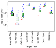
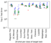
Fine-tuning with single-domain experts in model zoo. For fine-tuning, Imagenet pre-training is a standard technique. Note, most deep learning frameworks, e.g. PyTorch3, MxNet/Gluon etc., just have the Imagenet pre-trained models for different architectures in their model zoo. fig:finetune_full shows the top-1 test error obtained by fine-tuning single-domain experts in our model zoo vs. Imagenet expert.

Our fine-tuning hyper-parameters are: $30$ epochs, weight decay of $10^{-4}$, SGD with Nesterov momentum $0.9$, batch size of $32$ and learning rate decay by $0.1\times$ at $15$ and $25$ epochs. We observe that the most important hyper-parameter for test accuracy is the initial learning rate $\eta$, so for each fine-tuning we try $\eta=0.01$, $0.005$, $0.001$ and report the best top-1 test accuracy.

Does fine-tuning with model zoo perform better than fine-tuning a Imagenet expert? While fine-tuning an Imagenet pre-trained model is standard and works well on most target tasks, we show that by fine-tuning models of a large model-zoo we can indeed obtain a lower test error on some target tasks (see models highlighted by black $\leftarrow$ in fig:finetune_full). The reduction in error is more pronounced in the low-data regime. Therefore, we establish that maintaining a model zoo of models trained on different datasets is helpful to transfer to a diverse set of target tasks with different amounts of training data.

We demonstrate gains in the low-data regime by training on a smaller subset of the target task, with only 20, 5 samples per class in fig:finetune_full (i.e., we train in a 20-shot and 5-shot setting). In few-shot cases we still test on the full test set.

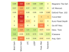
Fine-tuning with multi-domain expert. In sec:model_zoo, we show that fine-tuning can be done by choosing different domain-specific parameters within the multi-domain expert for fine-tuning. In fig:finetune_universal, we fine-tune the multi-domain expert, i.e. Multi-BN of tab:multi_domain, on our target tasks by choosing different domain-specific parameters to fine-tune. Similar to fig:finetune_full, we show the accuracy gain obtained by fine-tuning multi-domain expert with respect to fine-tuning the standard Resnet-101 pre-trained on Imagenet. We observe that selecting the correct domain to fine-tune, i.e. the correct $w_{d}$, where $d\in\{1,2,\cdots,D\}$ from multi-domain model zoo $\mathcal{F}=\{f_{w_{s},w_{d}}\}_{d=1}^{D}$, is important to obtain high fine-tuning test accuracy on the target task. In sec:model_selection, we show that model selection algorithms help in selecting the optimal domain-specific parameters for fine-tuning our multi-domain model zoo.

We also observe that fine-tuning with our multi-domain expert improves over the fine-tuning of single-domain model zoo for some tasks, e.g. iCassava: $+1.4\%$ accuracy gain with multi-domain expert compared to $+.72\%$ accuracy gain with single domain model expert over Imagenet expert. However, the comparison between single domain and multi-domain experts and their transfer properties is not the focus of our research and we refer the reader to [32, 44, 45].

Shots	Brute-force	Fine-tuning top-3 models					Model selection from single-domain model zoo
		LFC	LGC	LEEP	Feat. Met.	Dom. Sim.	LFC	LGC	LEEP	Feat. Met.	Dom. Sim.
Full	48.17$\times$	5.15$\times$	3.89$\times$	5.01$\times$	6.02$\times$	4.87$\times$	.41$\times$	8.65$\times$	.02$\times$	.00$\times$	.40$\times$
20-shot	41.67$\times$	4.35$\times$	3.40$\times$	3.85$\times$	4.86$\times$	4.11$\times$	1.09$\times$	15.26$\times$	0.03$\times$	0.00$\times$	1.31$\times$

Table 3: Computation cost of model selection and fine-tuning the selected models from single-domain model zoo. We measure the average run-time for all our target tasks (of fig:finetune_full) of: Brute-force fine-tuning and Fine-tuning with 3 models chosen by model selection (fig:model_zoo_selection_top3). We divide the run-time by the run-time of fine-tuning a Resnet-101 Imagenet expert. For the single domain model zoo, brute-force fine-tuning of all $30$ experts requires $40\times$ more computation than fine-tuning Imagenet Resnet-101 expert. Note, Densenet-169 models in our model zoo need more computation to fine-tune than Resnet-101, therefore the gain is $>30\times$ for our model zoo size of $30$. With model selection, we can fine-tune with selected models in only $3-6\times$ the computation. LFC and LEEP compute model selection scores for $30$ models in our zoo with $<1\times$ the computation of fine-tuning Imagenet Resnet-101 expert. LGC model selection is expensive due to backward passes and large dimension of the gradient vector. However, our LFC approximation to LGC is good at selecting models (fig:model_zoo_selection_top3) and fast.

4.3 Model Selection

(a) Selections for best model

(b) Spearman correlation of expert ranking using model selection scores to actual ranking using fine-tuning accuracy

Figure 6: In $(a)$, we measure the number of trials to select the best model, i.e. highest accuracy, from the model zoo. LFC, LGC and LEEP [37] require fewer trials than Domain Similarity [11], RSA [15] and Random selection baselines. In $(b)$, we show that model selection scores of LFC obtain the highest Spearman’s ranking correlation to the actual fine-tuning accuracy compared to other model selection methods. Model selection scores are proxy for fine-tuning accuracy, therefore high correlation is desirable.

In sec:finetune, using our benchmark we find that fine-tuning with a model zoo, both single-domain and multi-domain domain, improves the test accuracy on the target tasks. Now, we demonstrate that using a model selection algorithm we can select the best model or domain-specific parameters from our model zoos with only a few selections or trials.

Model Selection Algorithms. We use the following scores, $S$, for our model selection methods: LFC (see $S_{\text{LF}}$ defined in sec:implementation), LGC (see $S_{\text{LG}}$ defined in  (8)), which we introduce in sec:label-correlation. We compare against alternative measures of model selection and/or task similarity proposed in the literature: Domain similarity [11], Feature metrics [49], LEEP [37] and RSA [15]. Finally, we compare with a simple baseline: Random which selects models randomly for fine-tuning.

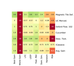
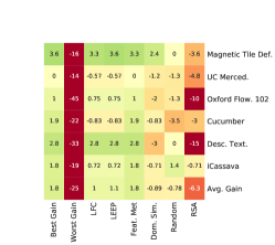
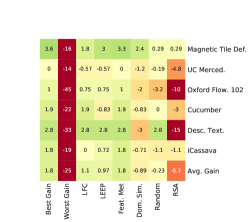
Model selection with single-domain model zoo. In fig:model_zoo_selection_top3, we select the top-$3$ experts (i.e. $3$ highest model selection scores) for each model selection method for fine-tuning. We do this for all the target tasks (row) using each model selection method (column). We use the maximum of fine-tuning test accuracy obtained by $3$ selected models to compute accuracy gain with respect to fine-tuning with Resnet-101 Imagenet expert. Ideally, we want the accuracy gain with the model selection method to be high and equal to the “Best Gain” possible for the target task. As seen in fig:model_zoo_selection_top3: LFC, LGC and LEEP obtain high accuracy gain with just 3 selections in both full dataset and 20-shot per class setting. They outperform random selection.

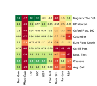
Model selection with multi-domain expert. For our multi-domain expert ( sec:model_zoo), we use model selection to select the domain-specific parameters to fine-tune for every model selection method. We compute the accuracy gain for fine-tuning using selected domains vs. fine-tuning Imagenet parameters in the multi-domain expert. It is desirable to have high or close to best gain with model selection. Our results in fig:universal_selection_top1, show that LFC and LEEP [37] obtain higher accuracy gain compared to Feature Metrics [49] and Random selection.

Is fine-tuning with model selection faster than brute-force fine-tuning? In tab:runtime, we show that brute-force fine-tuning is expensive. We can save computation by performing model selection using LFC and LEEP and fine-tuning only the selected top-$3$ models.

How many trials to select the model with best fine-tuning accuracy? In fig:trials, we measure the average of selections or trials, across all target tasks, required to select the best model for fine-tuning from the model zoo. The best model corresponds to the highest fine-tuning test accuracy on target task. Our label correlation and LEEP [37] methods can select the best model in $<7$ trials for our single domain model zoo of $30$ experts and in $<3$ trials for the multi-domain model zoo with $8$ domain experts.

Are model selection scores a good proxy for fine-tuning accuracy? In fig:trials, we show our LFC scores have the highest Spearman’s ranking correlation to the actual fine-tuning accuracy for different experts. Note, we average the correlation for all our target tasks. Our LFC score is a good proxy for ranking by fine-tuning accuracy and it can allow us to select (or reject) models for fine-tuning.

5 Conclusions

Fine-tuning using model zoo is a simple method to boost accuracy. We show that while a model zoo may have modest gains in the high-data regime, it outperforms Imagenet experts networks in the low-data regime. We show that simple baseline methods derived from a linear approximation of fine-tuning – Label-Gradient Correlation (LGC) and Label-Feature Correlation (LFC) – can select good models (single-domain) or parameters (multi-domain) to fine-tune, and match or outperform relevant model selection methods in the literature. Our model selection saves the cost of brute-force fine-tuning and makes model zoos viable.

Dataset	Training Images	Testing Images	# Classes	URL
NWPU-RESISC45 [7]	25,200	6300	45	https://www.tensorflow.org/datasets/catalog/resisc45
Food-101 [6]	75,750	25,250	101	https://www.tensorflow.org/datasets/catalog/food101
Logo 2k [50]	134,907	32,233	2341	https://github.com/msn199959/Logo-2k-plus-Dataset
Goog. Landmark [39]	200,000	15,601	256	https://github.com/cvdfoundation/google-landmark
iNaturalist [21]	265,213	3030	1010	https://github.com/visipedia/inat_comp
iMaterialist [33]	965,782	9639	2019	https://github.com/malongtech/imaterialist-product-2019
Imagenet [13]	1,281,167	50,000	1000	http://image-net.org/download
Places-365 [57]	1,803,460	36,500	365	http://places2.csail.mit.edu/download.html
Magnetic Tile Defects [23]	1008	336	6	https://github.com/abin24/Magnetic-tile-defect-datasets
UC Merced Land Use [53]	1575	525	21	http://weegee.vision.ucmerced.edu/datasets/landuse.html
Oxford Flowers 102 [38]	2040	6149	102	https://www.robots.ox.ac.uk/~vgg/data/flowers/102/
Cucumber [12]	2326	597	30	https://github.com/workpiles/CUCUMBER-9
European Flood Depth [5]	3153	557	2	https://github.com/cvjena/eu-flood-dataset
Oxford-IIIT Pets [41]	3680	3669	37	https://www.robots.ox.ac.uk/~vgg/data/pets/
Describable Textures [9]	4230	1410	47	https://www.robots.ox.ac.uk/~vgg/data/dtd/
iCassava [36]	5367	280	5	https://sites.google.com/view/fgvc6/competitions/icassava-2019
CUB-200 [52]	5994	5793	200	http://www.vision.caltech.edu/visipedia/CUB-200-2011.html
Belga Logos [25]	7500	2500	27	http://www-sop.inria.fr/members/Alexis.Joly/BelgaLogos/BelgaLogos.html
Stanford Cars [27]	8144	8041	196	https://ai.stanford.edu/~jkrause/cars/car_dataset.html

Table 4: The number of training images, testing images and classes as well as the URL to download the dataset are listed above. The top part contains our source datasets used to train the model zoo and the bottom part lists our target tasks used for fine-tuning and model selection with our model zoo.

Appendix A Proofs

Proof of Proposition 1. The proof follows easily from [29]. We summarize the steps to make the section self contained. Assuming, as we do, that the network is trained with a gradient flow (which is the continuous limit of gradient descent for small learning rate), then the weights and activations of the linearized model satisfies the differential equation:

$$\dot{w}_{t} =-\eta\nabla_{w}f_{w}(\mathcal{X})^{T}\nabla_{f_{y}(\mathcal{X})}\mathcal{L}$$

$$\dot{f}_{t}(\mathcal{X}) =-\eta\nabla_{w}f_{w}(\mathcal{X})^{T}\nabla_{f_{y}(\mathcal{X})}\mathcal{L}=-\eta\Theta\nabla_{f_{y}(\mathcal{X})}\mathcal{L}$$

For the MSE loss $\mathcal{L}:=\sum_{i=1}^{N}(y_{i}-f_{t}^{\text{lin}}(x_{i}))^{2}$, the second differential equations become a first order linear differential equation, which we can easily solve in close form. The solution is

$$f_{t}^{\text{lin}}(\mathcal{X})=(I-e^{-\eta\Theta t})\mathcal{Y}+e^{-\eta\Theta t}f_{0}(\mathcal{X}).$$

Putting this result in the expression for the loss at time $t$ gives

$$\mathcal{L}_{t} =\sum_{i=1}^{N}(y_{i}-f_{t}^{\text{lin}}(x_{i}))^{2}$$

$$=(\mathcal{Y}-f_{t}^{\text{lin}}(\mathcal{X}))^{T}(\mathcal{Y}-f_{t}^{\text{lin}}(\mathcal{X}))$$

$$=(\mathcal{Y}-f_{w_{0}}(\mathcal{X}))^{T}e^{-\eta\Theta t}(\mathcal{Y}-f_{w_{0}}(\mathcal{X})),$$

as we wanted.

Proof of using feature approximation in kernel. Using the notation $\mathbb{E}_{i,j}[a_{ij}]:=\frac{1}{N^{2}}\sum_{i,j=1}^{N}a_{ij}$ we have

$$\mathcal{Y}^{T}\,\Theta\,\mathcal{Y} =N^{2}\mathbb{E}_{i,j}[y_{i}y_{j}\Theta_{ij}]$$

$$=N^{2}\mathbb{E}_{i,j}[y_{i}y_{j}\nabla_{w}f_{w}(x_{i})\cdot\nabla_{w}f_{w}(x_{j})]$$

Now let’s consider an $f_{w}$ in the form of a DNN, that is $f_{w}(x)=W_{L}\phi(W_{L-1}\ldots\phi(W_{0}x))$. By the chain rule, the gradient of the weights at layer $l$ is given by:

$$\nabla_{W_{l}}f_{w}(x)=J_{l+1}(x)\otimes f^{l}_{w}(x)$$

where $J_{l+1}$ is the gradient of the output pre-activations coming from the upper layer and $f^{l}_{w}(x)$ are the input activations at layer $l$ and “$\otimes$” denotes the Kronecker’s product or, equivalently since both are vectors, the outer product of the two vectors. Recall that $\|A\otimes B\|_{2}=\|A\|_{2}\|B\|_{2}$, which will be useful later. Using this, we can rewrite $\mathcal{Y}^{T}\,\Theta\,\mathcal{Y}$ as follows:

$$\mathcal{Y}^{T}\,\Theta\,\mathcal{Y}$$

$$=N^{2}\mathbb{E}_{i,j}[y_{i}y_{j}\nabla_{w}f_{w}(x_{i})\cdot\nabla_{w}f_{w}(x_{j})]$$

$$=N^{2}\mathbb{E}_{i}[y_{i}\nabla_{w}f_{w}(x_{i})]\cdot\mathbb{E}_{j}[y_{j}\nabla_{w}f_{w}(x_{j})]$$

$$=N^{2}\sum_{l=1}^{L}\mathbb{E}_{i}[y_{i}J_{l+1}(x_{i})\otimes f^{l}_{w}(x_{i})]\cdot\mathbb{E}_{j}[y_{j}J_{l+1}(x_{j})\otimes f^{l}_{w}(x_{j})]$$

We now introduce a further approximation and assume that $J_{l+1}$ is uncorrelated from $f^{l}_{w}(x_{i})$. The same assumption is used by [34] (see Section 3.1) who also provide theoretical and empirical justifications. Using this assumption, we have:

$$\mathcal{Y}^{T}\,\Theta\,\mathcal{Y} =N^{2}\sum_{l=1}^{L}\Big{\|}\mathbb{E}_{i}[y_{i}J_{l+1}(x_{i})\otimes f^{l}_{w}(x_{i})]]\Big{\|}^{2}$$

$$=N^{2}\sum_{l=1}^{L}\Big{\|}\mathbb{E}_{i}[J_{l+1}(x_{i})]\otimes\mathbb{E}_{i}[y_{j}f^{l}_{w}(x_{j})]\Big{\|}^{2}$$

$$=N^{2}\sum_{l=1}^{L}\Big{\|}\mathbb{E}_{i}[J_{l+1}(x_{i})]\Big{\|}^{2}\Big{\|}\mathbb{E}_{i}[y_{j}f^{l}_{w}(x_{j})]\Big{\|}^{2}$$

The term $\mathbb{E}_{i}[y_{j}f^{l}_{w}(x_{j})]$ measures the correlation between each individual feature and the label. If features are correlated with labels, then $\mathcal{Y}^{T}\,\Theta\,\mathcal{Y}$ is larger, and hence initial convergence is faster. Note that we need not consider only the last layer, convergence speed is determined by the correlation at all layers. Note however that the contribution of earlier layers is discounted by a factor of $\|\mathbb{E}_{i}[J_{l+1}(x_{i})]\|^{2}$. As we progress further down the network, the average of the gradients may become increasingly smaller, decreasing the term $\|\mathbb{E}_{i}[J_{l+1}(x_{i})]\|^{2}$ and hence diminishing the contribution of earlier layer clustering to convergence speed.

Appendix B Datasets

We choose our source and target datasets such that they cover different domains, and are publicly available for download. Detailed data statistics are in the respective citations for the datasets, and we include a few statistics e.g. training images, testing images, number of classes in tab:suppl_datasets. For all the datasets, if available we use the standard train and test split of the dataset, else we split the dataset randomly into 80% train and 20% test images. If images are indexed by URLs in the dataset, we download all accessible URLs with a python script.

Appendix C Details of model selection methods

(a) 25 samples per class

(b) 50 samples per class

(c) Full target task

Figure 7: Ablation study of dataset size for model selection. Above we use 25,50-samples per class and full target task to perform model selection with different methods. We plot accuracy gain vs. Imagenet expert for top-3 selected models for every method (similar to Fig. 4 of the paper). The accuracy gain increases for LFC, LEEP and RSA with more samples of the target task. However, we see that even as small as $25$ samples suffice to obtain good accuracy gain with low computational cost.

(a) NWPU-RESISC45, Epoch=0

(b) NWPU-RESIC45, Epoch=15

(c) NWPU-RESISC45, Epoch=30

(d) Food-101, Epoch=0

(e) Food-101, Epoch=15

(f) Food-101, Epoch=30

(g) Logo 2k, Epoch=0

(h) Logo 2k, Epoch=15

(i) Logo 2k, Epoch=30

Figure 8: We plot the feature correlation matrix, $\Theta_{F}$, for different pre-trainings (row) and different epochs (columns) of fine-tuning. Above, we fine-tune on the UC Merced Land Use [53] dataset comprising of aerial images. Images with same class label, 25 images per class, are grouped along the vertical/horizontal axis. Since, features of the same class should be correlated and features of different classes should be uncorrelated, the matrix is expected to have higher values along block diagonal and zero elsewhere. We observe that the matrix exhibits this ideal behaviour for pre-training on semantically related domain (aerial images) of NWPU-RESISC45 [7] (top row) and has highest LFC score for this pre-training.

Domain Similarity [11]. As per  [11], we extract avg. features for every class for source and target datasets using pre-trained model. We compute an earth movers distance between these average class vectors and convert them to domain similarity score. We use the code provided by the authors at https://github.com/richardaecn/cvpr18-inaturalist-transfer. We exclude classes with less than $5$ training images for Earth-Movers Distance computation.

RSA [15]. Following the procedure outlined in [15], we extract features before the classification layer (e.g. 2048 dim features of Resnet-101 after average pool) for images in the target dataset. We denote this set of features as $f(x)$, $\forall(x,y)\in\mathcal{D}$. We build a representation dissimilarity matrix (RDM) as follows:

$$\text{rdm}_{f}(i,j)=1-correlation(f(x_{i}),f(x_{j}))$$ (9)

We train a small neural network $f_{\text{small}}$ on target dataset. Note, this is much cheaper to train than fine-tuning the model zoo. Features are extracted from $f_{\text{small}}$ and we build another rdm:

$$\text{rdm}_{f_{\text{small}}}(i,j)=1-correlation(f_{\text{small}}(x_{i}),f_{\text{small}}(x_{j}))$$ (10)

If rdm’s of trained small network $f_{\text{small}}$ and our pre-trained model $f$ are similar, then the pre-trained model is a good candidate for fine-tuning with target dataset. The final RSA model selection score is:

$$S_{\text{RSA}}(f,\mathcal{D})=\text{spearmanr}(\text{rdm}_{f},\text{rdm}_{f_{\text{small}}})$$ (11)

Since the method requires training a small neural network on target task, we train a Resnet-18 as the small neural network with the same fine-tuning configuration used in Section 4.1 of the paper with initial learning rate = $.005$.

Feature Metrics [49]. Features are extracted for all images of target dataset from pre-trained model, i.e. $f(x),\forall x\in\mathcal{D}$. We use same features as RSA, our LFC/LGC and compute variance, sparsity metrics of  [49]. We use the sparsity metrics as model selection score, $S_{\text{Feat. Metrics}}(f,\mathcal{D})=\text{sparsity}({f(x),\forall x\in\mathcal{D}})$. Note, we use the optimal linear combination of the two sparsity metrics proposed in the paper. For feature metrics, the hypothesis is that if the pre-trained model generates more sparse representations, they are can generalize with fine-tuning to the target task.

LEEP [37]. LEEP builds an empirical classifier from source dataset label space to target dataset label space using base model $f$. The likelihood of target dataset $\mathcal{D}$ under this empirical classifier is the model selection score for the pre-trained model and target dataset. See [37] for a detailed explanation.

Appendix D Different dataset size for model selection

In fig:model_selection_dataset_size, we perform an ablation study on different sampling size of the target task used for model selection. We find that, our choice of $25$ samples per class for model selection, suffices to select good models to fine-tune in top-3 selections at low-computational cost.

Appendix E Visualization of $\Theta_{F}$ with fine-tuning

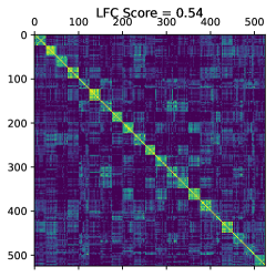
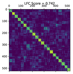
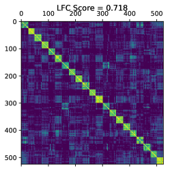
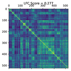
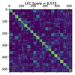
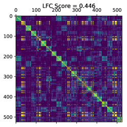
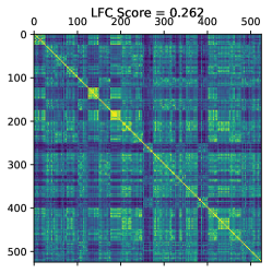
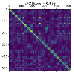
In fig:rdm_visualize, we plot the feature correlation matrix for different pre-trained models across different epochs of fine-tuning (i.e. $0^{th}$, $15^{th}$, $30^{th}$ epoch) for the UC Merced Land Use [53] target task. We see that the pre-trained model on NWPU-RESISC45 [7], exhibits the ideal correlation wherein features of the images with the same class are correlated and features of images with different classes are uncorrelated. This NWPU-RESISC45 [7] also has the highest LFC score.

References

- [1] Alessandro Achille, Michael Lam, Rahul Tewari, Avinash Ravichandran, Subhransu Maji, Charless C Fowlkes, Stefano Soatto, and Pietro Perona. Task2vec: Task embedding for meta-learning. In Proceedings of the IEEE International Conference on Computer Vision, pages 6430–6439, 2019.
- [2] Alessandro Achille, Giovanni Paolini, Glen Mbeng, and Stefano Soatto. The Information Complexity of Learning Tasks, their Structure and their Distance. arXiv e-prints, page arXiv:1904.03292, Apr 2019.
- [3] Sanjeev Arora, Simon Du, Wei Hu, Zhiyuan Li, and Ruosong Wang. Fine-grained analysis of optimization and generalization for overparameterized two-layer neural networks. In International Conference on Machine Learning, pages 322–332, 2019.
- [4] Bjorn Barz and Joachim Denzler. Deep learning on small datasets without pre-training using cosine loss. In The IEEE Winter Conference on Applications of Computer Vision, pages 1371–1380, 2020.
- [5] Björn Barz, Kai Schröter, Moritz Münch, Bin Yang, Andrea Unger, Doris Dransch, and Joachim Denzler. Enhancing flood impact analysis using interactive retrieval of social media images. ArXiv, abs/1908.03361, 2019.
- [6] Lukas Bossard, Matthieu Guillaumin, and Luc Van Gool. Food-101 – mining discriminative components with random forests. In European Conference on Computer Vision, 2014.
- [7] G. Cheng, J. Han, and X. Lu. Remote sensing image scene classification: Benchmark and state of the art. Proceedings of the IEEE, 105(10):1865–1883, 2017.
- [8] G. Cheng, J. Han, and X. Lu. Remote sensing image scene classification: Benchmark and state of the art, 2017.
- [9] M. Cimpoi, S. Maji, I. Kokkinos, S. Mohamed, , and A. Vedaldi. Describing textures in the wild. In Proceedings of the IEEE Conf. on Computer Vision and Pattern Recognition (CVPR), 2014.
- [10] Yin Cui, Yang Song, Chen Sun, Andrew Howard, and Serge Belongie. Large scale fine-grained categorization and domain-specific transfer learning. In Proceedings of the IEEE conference on computer vision and pattern recognition, pages 4109–4118, 2018.
- [11] Yin Cui, Yang Song, Chen Sun, Andrew Howard, and Serge Belongie. Large scale fine-grained categorization and domain-specific transfer learning. In CVPR, 2018.
- [12] Cucumber-9 dataset. https://github.com/workpiles/cucumber-9.
- [13] J. Deng, W. Dong, R. Socher, L.-J. Li, K. Li, and L. Fei-Fei. ImageNet: A Large-Scale Hierarchical Image Database. In CVPR09, 2009.
- [14] Nikita Dvornik, Cordelia Schmid, and Julien Mairal. Selecting relevant features from a universal representation for few-shot classification. arXiv preprint arXiv:2003.09338, 2020.
- [15] Kshitij Dwivedi and Gemma Roig. Representation similarity analysis for efficient task taxonomy & transfer learning. In IEEE Conference on Computer Vision and Pattern Recognition, CVPR 2019, Long Beach, CA, USA, June 16-20, 2019, pages 12387–12396. Computer Vision Foundation / IEEE, 2019.
- [16] Micah Goldblum, Jonas Geiping, Avi Schwarzschild, Michael Moeller, and Tom Goldstein. Truth or backpropaganda? an empirical investigation of deep learning theory. arXiv preprint arXiv:1910.00359, 2019.
- [17] Pavel Golik, Patrick Doetsch, and Hermann Ney. Cross-entropy vs. squared error training: a theoretical and experimental comparison. In Interspeech, volume 13, pages 1756–1760, 2013.
- [18] Priya Goyal, Dhruv Mahajan, Abhinav Gupta, and Ishan Misra. Scaling and benchmarking self-supervised visual representation learning. 2019.
- [19] K. He, X. Zhang, S. Ren, and J. Sun. Deep residual learning for image recognition. In 2016 IEEE Conference on Computer Vision and Pattern Recognition (CVPR), pages 770–778, 2016.
- [20] Kaiming He, Ross Girshick, and Piotr Dollár. Rethinking imagenet pre-training. In Proceedings of the IEEE International Conference on Computer Vision, pages 4918–4927, 2019.
- [21] Grant Van Horn, Oisin Mac Aodha, Yang Song, Alexander Shepard, Hartwig Adam, Pietro Perona, and Serge J. Belongie. The inaturalist challenge 2017 dataset. CoRR, abs/1707.06642, 2017.
- [22] Gao Huang, Zhuang Liu, and Kilian Q. Weinberger. Densely connected convolutional networks. CoRR, abs/1608.06993, 2016.
- [23] Y. Huang, C. Qiu, Y. Guo, X. Wang, and K. Yuan. Surface defect saliency of magnetic tile. In 2018 IEEE 14th International Conference on Automation Science and Engineering (CASE), pages 612–617, 2018.
- [24] Arthur Jacot, Franck Gabriel, and Clément Hongler. Neural tangent kernel: Convergence and generalization in neural networks. In Advances in neural information processing systems, pages 8571–8580, 2018.
- [25] Alexis Joly and Olivier Buisson. Logo retrieval with a contrario visual query expansion. In MM ’09: Proceedings of the seventeen ACM international conference on Multimedia, pages 581–584, 2009.
- [26] Alexander Kolesnikov, Lucas Beyer, Xiaohua Zhai, Joan Puigcerver, Jessica Yung, Sylvain Gelly, and Neil Houlsby. Big transfer (bit): General visual representation learning. In Andrea Vedaldi, Horst Bischof, Thomas Brox, and Jan-Michael Frahm, editors, Computer Vision – ECCV 2020, pages 491–507, Cham, 2020. Springer International Publishing.
- [27] Jonathan Krause, Michael Stark, Jia Deng, and Li Fei-Fei. 3d object representations for fine-grained categorization. In 4th International IEEE Workshop on 3D Representation and Recognition (3dRR-13), Sydney, Australia, 2013.
- [28] Alex Krizhevsky. Learning multiple layers of features from tiny images. Technical report, 2009.
- [29] Jaehoon Lee, Lechao Xiao, Samuel S. Schoenholz, Yasaman Bahri, Roman Novak, Jascha Sohl-Dickstein, and Jeffrey Pennington. Wide neural networks of any depth evolve as linear models under gradient descent, 2019.
- [30] Jungkyu Lee, Taeryun Won, Tae Kwan Lee, Hyemin Lee, Geonmo Gu, and Kiho Hong. Compounding the performance improvements of assembled techniques in a convolutional neural network, 2020.
- [31] Hao Li, Pratik Chaudhari, Hao Yang, Michael Lam, Avinash Ravichandran, Rahul Bhotika, and Stefano Soatto. Rethinking the hyperparameters for fine-tuning. In ICLR, 2020.
- [32] A. Mallya and S. Lazebnik. Packnet: Adding multiple tasks to a single network by iterative pruning. In 2018 IEEE/CVF Conference on Computer Vision and Pattern Recognition, pages 7765–7773, 2018.
- [33] MalongTech. Imaterialist dataset, https://github.com/malongtech/imaterialist-product-2019.
- [34] James Martens and Roger Grosse. Optimizing neural networks with kronecker-factored approximate curvature. In International conference on machine learning, pages 2408–2417, 2015.
- [35] Fangzhou Mu, Yingyu Liang, and Yin Li. Gradients as features for deep representation learning. arXiv preprint arXiv:2004.05529, 2020.
- [36] Ernest Mwebaze, Timnit Gebru, Andrea Frome, Solomon Nsumba, and Jeremy Tusubira. icassava 2019 fine-grained visual categorization challenge, 2019.
- [37] Cuong V Nguyen, Tal Hassner, Cedric Archambeau, and Matthias Seeger. Leep: A new measure to evaluate transferability of learned representations. arXiv preprint arXiv:2002.12462, 2020.
- [38] M. Nilsback and A. Zisserman. Automated flower classification over a large number of classes. In 2008 Sixth Indian Conference on Computer Vision, Graphics Image Processing, pages 722–729, 2008.
- [39] H. Noh, A. Araujo, J. Sim, T. Weyand, and B. Han. Large-scale image retrieval with attentive deep local features. In 2017 IEEE International Conference on Computer Vision (ICCV), pages 3476–3485, 2017.
- [40] PapersWithCode. See https://paperswithcode.com/sota/image-classification-on-inaturalist for more details.
- [41] Omkar M. Parkhi, Andrea Vedaldi, Andrew Zisserman, and C. V. Jawahar. Cats and dogs. In IEEE Conference on Computer Vision and Pattern Recognition, 2012.
- [42] Adam Paszke, Sam Gross, Francisco Massa, Adam Lerer, James Bradbury, Gregory Chanan, Trevor Killeen, Zeming Lin, Natalia Gimelshein, Luca Antiga, Alban Desmaison, Andreas Kopf, Edward Yang, Zachary DeVito, Martin Raison, Alykhan Tejani, Sasank Chilamkurthy, Benoit Steiner, Lu Fang, Junjie Bai, and Soumith Chintala. Pytorch: An imperative style, high-performance deep learning library. In H. Wallach, H. Larochelle, A. Beygelzimer, F. d'Alché-Buc, E. Fox, and R. Garnett, editors, Advances in Neural Information Processing Systems 32, pages 8024–8035. Curran Associates, Inc., 2019.
- [43] PyTorch. See https://pytorch.org/docs/stable/torchvision/models.html for more details.
- [44] S-A Rebuffi, H. Bilen, and A. Vedaldi. Learning multiple visual domains with residual adapters. In Advances in Neural Information Processing Systems, 2017.
- [45] Sylvestre-Alvise Rebuffi, Hakan Bilen, and Andrea Vedaldi. Efficient parametrization of multi-domain deep neural networks. 2018.
- [46] Anh T Tran, Cuong V Nguyen, and Tal Hassner. Transferability and hardness of supervised classification tasks. In Proceedings of the IEEE International Conference on Computer Vision, pages 1395–1405, 2019.
- [47] Eleni Triantafillou, Tyler Zhu, Vincent Dumoulin, Pascal Lamblin, Utku Evci, Kelvin Xu, Ross Goroshin, Carles Gelada, Kevin Swersky, Pierre-Antoine Manzagol, et al. Meta-dataset: A dataset of datasets for learning to learn from few examples. arXiv preprint arXiv:1903.03096, 2019.
- [48] Eleni Triantafillou, Tyler Zhu, Vincent Dumoulin, Pascal Lamblin, Utku Evci, Kelvin Xu, Ross Goroshin, Carles Gelada, Kevin Jordan Swersky, Pierre-Antoine Manzagol, and Hugo Larochelle. Meta-dataset: A dataset of datasets for learning to learn from few examples. In International Conference on Learning Representations (submission), 2020.
- [49] Yosuke Ueno and Masaaki Kondo. A base model selection methodology for efficient fine-tuning, 2020.
- [50] J. Wang, W. Min, S. Hou, S. Ma, Y. Zheng, H. Wang, and S. Jiang. Logo-2k+: A large-scale logo dataset for scalable logo classification. 2019. .
- [51] Jing Wang, Weiqing Min, Sujuan Hou, Shengnan Ma, Yuanjie Zheng, Haishuai Wang, and Shuqiang Jiang. Logo-2k+: A large-scale logo dataset for scalable logo classification, 2019.
- [52] P. Welinder, S. Branson, T. Mita, C. Wah, F. Schroff, S. Belongie, and P. Perona. Caltech-UCSD Birds 200. Technical Report CNS-TR-2010-001, California Institute of Technology, 2010.
- [53] Yi Yang and Shawn Newsam. Bag-of-visual-words and spatial extensions for land-use classification. In Proceedings of the 18th SIGSPATIAL International Conference on Advances in Geographic Information Systems, GIS ’10, page 270–279, New York, NY, USA, 2010. Association for Computing Machinery.
- [54] Amir R Zamir, Alexander Sax, William Shen, Leonidas J Guibas, Jitendra Malik, and Silvio Savarese. Taskonomy: Disentangling task transfer learning. In Proceedings of the IEEE Conference on Computer Vision and Pattern Recognition, pages 3712–3722, 2018.
- [55] Amir R Zamir, Alexander Sax, William B Shen, Leonidas Guibas, Jitendra Malik, and Silvio Savarese. Taskonomy: Disentangling task transfer learning. In 2018 IEEE Conference on Computer Vision and Pattern Recognition (CVPR). IEEE, 2018.
- [56] Luca Zancato, Alessandro Achille, Avinash Ravichandran, Rahul Bhotika, and Stefano Soatto. Predicting training time without training, 2020.
- [57] Bolei Zhou, Agata Lapedriza, Aditya Khosla, Aude Oliva, and Antonio Torralba. Places: A 10 million image database for scene recognition. IEEE Transactions on Pattern Analysis and Machine Intelligence, 2017.
- [58] Barret Zoph, Golnaz Ghiasi, Tsung-Yi Lin, Yin Cui, Hanxiao Liu, Ekin D. Cubuk, and Quoc V. Le. Rethinking pre-training and self-training, 2020.