Network-centric indicators for fragility in global financial indices

Abstract

Over the last two decades, financial systems have been studied and analysed from the perspective of complex networks, where the nodes and edges in the network represent the various financial components and the strengths of correlations between them. Here, we adopt a similar network-based approach to analyse the daily closing prices of 69 global financial market indices across 65 countries over a period of 2000-2014. We study the correlations among the indices by constructing threshold networks superimposed over minimum spanning trees at different time frames. We investigate the effect of critical events in financial markets (crashes and bubbles) on the interactions among the indices by performing both static and dynamic analyses of the correlations. We compare and contrast the structures of these networks during periods of crashes and bubbles, with respect to the normal periods in the market. In addition, we study the temporal evolution of traditional market indicators, various global network measures and the recently developed edge-based curvature measures. We show that network-centric measures can be extremely useful in monitoring the fragility in the global financial market indices.

1 Introduction

It is possible to describe a financial market using the framework of complex networks such that the nodes in a network represent the financial components and an edge between any two components indicates an interaction between them. A correlation matrix constructed using the cross-correlations of fluctuations in prices can be utilized to identify such interactions. However, a network resulting from the correlation matrix contains densely connected structures. A growing amount of research is focused on methods devised to extract relevant correlations from the correlation matrix and study the topological, hierarchical and clustering properties of the resulting networks. Mantegna et al. Mantegna (1999a, b) introduced the minimum spanning tree (MST) to extract networks from the correlation matrices computed from the asset returns. Dynamic asset trees, introduced by Onnela et al. Onnela et al. (2003a, 2004), were analysed to monitor the evolution of financial stock markets using the hierarchical clustering properties of such trees. Boginski et al. Boginski et al. (2005) constructed threshold networks by extracting the edges with correlation values exceeding a chosen threshold and analyzed degree distribution, cliques and independent sets on the threshold network. Tumminello et al. Tumminello et al. (2005) introduced planar maximally filtered graph (PMFG) as a tool to extract important edges from the correlation matrix, which contains more information than the MST, while also preserving the hierarchical structure induced by MST. Triangular loops and four-element cliques in PMFG could provide considerable insights into the structure of financial markets.

Network-based analysis has been widely used to study not only particular stock market structures but also the complex networks of correlations among different financial market indices across the globe. For example, MST has been used on stock markets to detect underlying hierarchical organization Bonanno et al. (2003); Onnela et al. (2003b); Bonanno et al. (2004). Bonanno et al. Bonanno et al. (2000) studied the correlations of 51 global financial indices and showed that the corresponding MST was clustered according to the geographical locations of the indices. In addition, the changes in the topological structure of MST could help understand the evolution of financial systems Nobi et al. (2014); Wang and He (2017); Coelho et al. (2007). MST and threshold networks have been used to analyse the indices during the global financial crisis of 2008 Kumar and Deo (2012); Junior et al. (2015); Lee and Nobi (2018). It has also been shown that geography is one of the major factors which govern the hierarchy of the global market León et al. (2017); Saeedian et al. (2019). Also, Eryǧit and Eryǧit Eryiğit and Eryiğit (2009) had investigated the temporal evolution of clustering networks (MST and PMFG) of 143 financial indices corresponding to 59 countries across the world from the period 1995-2008, and once again found that the clustering in the networks of financial indices was according to their geographical locations. From the time dependent network and centrality measures they showed that the integration of the global financial indices has increased with time. Further, Chen et al. Chen et al. (2020) analyzed dynamics of threshold networks of regional and global financial markets from the period 2012-2018, proposed a model for the measurement of systemic risk based on network topology and then concluded that network-based methods provide a more accurate measurement of systemic risk compared to the traditional absorption technique. Silva et al. Silva et al. (2016) studied the average criticality of countries during different periods in the crisis and found that the USA is the most critical country, followed by European countries, Oceanian and Asian countries, and finally Latin American countries and Canada . They also found a decrease in the network fragility after the global financial crisis. It has been also shown that financial crises can be captured using networks of volatility spillovers Baumohl et al. (2018); Mensi et al. (2018). Wang et al. Wang et al. (2018a) constructed and analysed dynamical structure of MSTs and hierarchical trees computed from the Pearson correlations as well as partial correlations, among 57 global financial markets from the period 2005-2014, and concluded that MST based on partial correlations provided more information when compared to MST based on Pearson correlations. The market indices from different stock markets across the globe comprise assets that are very different – apart from stocks of the big multinational companies that are traded across markets, the stock markets would have little in common, and hence would be expected to behave independently. However, all the aforementioned studies suggest in contrary.

In this brief research report, we study the evolution of correlation structures among 69 global financial indices through the years 2000 to 2014. To ensure that we consider only the most relevant correlations, we construct the network by creating an MST (which connects all the nodes) and then add extra edges from the correlation matrix exceeding a certain threshold, which gives modular structures. Our findings corroborate the earlier results of geographical clustering León et al. (2017); Sharma et al. (2019). We then study the changes occurring in the market by analysing the fluctuations in various global network measures and the recently developed edge-based geometric measures. Since there are complex interactions that occur among groups of three or more nodes, which cannot be described simply by pairwise interactions, the higher-order architecture of complex financial systems captured by the geometrical measures can help us in the betterment of systemic risk estimation and give us an indication of the global market efficiency. To the best of our knowledge, the present work is the first investigation of discrete Ricci curvatures in networks of global market indices. Thus, we find that this approach along with all these network measures can be used to monitor the fragility of the global financial network and as indicators of crashes and bubbles occurring in the markets. This could in turn relate the health of the financial markets with the development or downturn of the global economy, as well as gauge the impact of certain market crises in the multi-level financial-economic phenomena.

2 Methods

2.1 Data description

This study is based on a dataset collected from Bloomberg which comprises the daily closing prices of 69 global financial market indices from 65 countries, and this information was compiled for a period of $T=3513$ days over 14 years from 11 January 2000 to 24 June 2014. Note that the working days for different markets are not same due to differences in holidays across countries. To overcome any inconsistencies due to this difference in working days, we filtered the data by removing days on which $>30\%$ of the markets were not operative. Conversely, if $<30\%$ of the markets were not operative on a day, we used the closing price of such markets on the previous day to complete the dataset. Supplementary Table S1 lists the 69 global market indices considered here, along with their countries and geographical regions.

2.2 Cross-correlation matrix and market indicators

Given the daily closing price $g_{j}(t)$ for market index $j$ on day $t$, wherein $j=1,2,\ldots,N$ with $N=69$ indices, we construct a time series of logarithmic returns as $r_{j}(t)=\ln g_{j}(t)-\ln g_{j}(t-1)$. Then, we construct the equal time Pearson cross-correlation matrix as

$$C_{ij}^{\tau}(t)=\frac{\left\langle r_{i}r_{j}\right\rangle-\left\langle r_{i}\right\rangle\left\langle r_{j}\right\rangle}{\sigma_{i}\sigma_{j}},$$ (1)

where the mean and standard deviation are computed over a period of $\tau=80$ days with end date as $t$. We also construct the ultrametric distance matrix with elements $D_{ij}^{\tau}(t)=\sqrt{2(1-C_{ij}^{\tau}(t))}$ that take values between 0 and 2. To study the temporal dynamics of the global market indices, we computed the correlation matrices for overlapping windows of $\tau=80$ days with a rolling shift of $\Delta\tau=20$ days. Thence, we obtained $172$ correlation frames between 11 January 2000 to 24 June 2014.

We have computed three market indicators from these correlation matrices $\mathbf{C}^{\tau}(t)$. Firstly, the mean correlation gives the average of the correlations in the matrix $\mathbf{C}^{\tau}(t)$. Secondly, we have computed the eigen-entropy Chakraborti et al. (2020a) which involves calculation of the Shannon entropy using the eigenvector centralities of the correlation matrix $\mathbf{C}^{\tau}(t)$ of market indices. Both mean correlation and eigen-entropy has been shown to detect critical events in financial markets Chakraborti et al. (2020a, b); Kukreti et al. (2020). Thirdly, we have computed the risk corresponding to the Markowitz portfolio of the market indices, which is a proxy for the fragility or systemic risk of the global financial network Sandhu et al. (2016). A detailed description of the Markowitz portfolio optimization is given in the Supplementary Material.

2.3 Threshold network construction and characteristics

The distance matrix for the time frame ending on $t$ can be viewed as a complete, undirected and weighted graph $\mathbf{D}^{\tau}(t)$ where the element $D_{ij}^{\tau}(t)$ is the weight of the edge between market indices $i$ and $j$. To extract the important edges from $\mathbf{D}^{\tau}(t)$, we first construct its minimum spanning tree (MST) $\mathbf{M}^{\tau}(t)$ using Prim’s algorithm Prim (1957). As MST is an over-simplified network without cycles, it may lose crucial information on clusters or cliques. To overcome this, we add edges with correlation $C_{ij}^{\tau}\geq 0.65$ in $\mathbf{D}^{\tau}(t)$ to $\mathbf{M}^{\tau}(t)$ and obtain the threshold graph $\mathbf{S}^{\tau}(t)$. Thereafter, we study the temporal evolution of different network measures in $\mathbf{S}^{\tau}(t)$.

Firstly, we have computed standard global network measures such as the number of edges, edge density, average degree, average weighted degree Barrat et al. (2004), average shortest path length, diameter, average clustering coefficient Onnela et al. (2005), modularity Girvan and Newman (2002); Blondel et al. (2008), communication efficiency Latora and Marchiori (2001), global reaching centrality (GRC) Mones et al. (2012), network entropy Solé and Valverde (2004), global assortativity Newman (2003); Leung and Chau (2007) and clique number. Note that the chosen set of global network measures studied here are by no means exhaustive and also depend very much on the specific questions of interest, see for example, Wang et al. Wang et al. (2018b) for several gravitational centrality measures. Secondly, we have also computed four edge-centric curvature measures, namely, Ollivier-Ricci (OR) curvature Ollivier (2007); Sandhu et al. (2016); Samal et al. (2018), Forman-Ricci (FR) curvature Forman (2003); Sreejith et al. (2016); Samal et al. (2018); Saucan et al. (2019a), Menger-Ricci (MR) curvature Saucan et al. (2019b, 2020) and Haantjes-Ricci (HR) curvature Saucan et al. (2019b, 2020). A detailed description of these network measures along with the appropriate natural weight, strength or distance, to use in each case is included in the Supplementary Material.

2.4 Multidimensional scaling map

The multidimensional scaling (MDS) technique tries to embed $N$ objects in high-dimensional space into a low-dimensional space (typically, $2$- or $3$-dimensions), while preserving the relative distance between pairs of objects Borg and Groenen (2005). Here, we construct the (average) correlation matrix $\mathbf{C}^{T}$ between the 69 market indices for the complete period of $T=3513$ days between 11 January 2000 to 24 June 2014 using Eq. 1. Then, we compute the distance matrix $\mathbf{D}^{T}$ from $\mathbf{C}^{T}$ for the complete period. Thereafter, we use MDS to map the 69 market indices into a $2$-dimensional space such that the distances between pairs of indices in $\mathbf{D}^{T}$ are preserved. To create the MDS plot, we used the in-built function cmdscale.m in MATLAB. Moreover, we also construct the MST $\mathbf{M}^{T}$ starting from the distance matrix $\mathbf{D}^{T}$, and then, the threshold network $\mathbf{S}^{T}$ for the complete period from 2000 to 2014 by adding edges with $C_{ij}^{T}\geq 0.65$ to $\mathbf{M}^{T}$.

Figure 1: Evolution of generic indicators and network characteristics for the global market indices networks $\mathbf{S}^{\tau}(t)$, constructed from the correlation matrices $\mathbf{C}^{\tau}(t)$ of window size $\tau=80$ days and an overlapping shift of $\Delta\tau=20$ days over a period of 14 years (2000-2014). The threshold networks $\mathbf{S}^{\tau}(t)$ were constructed by adding edges with correlation $C_{ij}^{\tau}(t)\geq 0.65$ to the minimum spanning trees (MST). From top to bottom, we compare the plots of mean correlation among market indices, minimum risk corresponding to the Markowitz portfolio optimization, eigen-entropy, number of edges, average weighted degree, diameter, clustering coefficient, modularity, communication efficiency, global reaching centrality (GRC), network entropy and global assortativity. The four shaded regions correspond to the epochs around the four important market events, namely, US housing bubble, Lehman brothers crash, Dow Jones flash crash, and August 2011 stock markets fall.

Figure 2: Evolution of network characteristics and visualization of the threshold networks $\mathbf{S}^{\tau}(t)$ of market indices with window size $\tau=80$ days and an overlapping shift of $\Delta\tau=20$ days, constructed by adding edges with correlation $C_{ij}^{\tau}(t)\geq 0.65$ to the MST. (Lower panel) Comparison of the plots of mean correlation among market indices, clique number, average of Ollivier-Ricci (OR), Forman-Ricci (FR), Menger-Ricci (MR), and Haantjes-Ricci (HR) curvature of edges in threshold networks over the 14-year period. (Upper panel) Visualization of the threshold networks at three distinct epochs of $\tau=80$ days ending on trading days $t$ equal to 04-08-2005 (normal), 14-08-2006 (US housing bubble) and 04-06-2010 (Dow Jones flash crash). Threshold networks show higher number of edges and lower number of communities during crisis. Correspondingly, there is an increase in mean correlation, clique number, average OR, MR and HR curvature, and decrease in average FR curvature of threshold networks during financial crisis. Node colours and labels are based on geographical region and country, respectively, of the indices and edge colours are based on the community determined by Louvain method. The four USA market indices, NASDAQ, NYSE, RUSSELL1000 and SPX, are labelled as USA1, USA2, USA3 and USA4, respectively, while the two Indian indices, namely, NIFTY and SENSEX30, are labelled as IND1 and IND2, respectively.

Figure 3: Correlations between generic indicators and network characteristics of the global market indices networks $\mathbf{S}^{\tau}(t)$, constructed from the correlation matrices $\mathbf{C}^{\tau}(t)$ of window size $\tau=80$ days and an overlapping shift of $\Delta\tau=20$ days over a period of 14 years (2000-2014). The threshold networks $\mathbf{S}^{\tau}(t)$ were constructed by adding edges with correlation $C_{ij}^{\tau}(t)\geq 0.65$ to the minimum spanning tree (MST).

Figure 4: The average correlation structure between 69 market indices over the 14-year period is visualized based on the correlation matrix $\mathbf{C}^{T}$ for the complete period of $T=3513$ days between 2000 to 2014. (a) Visualization of the overall threshold network $\mathbf{S}^{T}$ corresponding to $\mathbf{C}^{T}$ obtained by combining MST plus edges with correlation $\geq 0.65$. The node colours are based on geographical regions of the market indices and edge colours are based on communities obtained from Louvain method. (b) Visualization of the communities in the overall threshold network $\mathbf{S}^{T}$ after removing the inter-module edges. It is evident that the market indices form communities in this network based on their geographical proximity. (c) Multidimensional scaling (MDS) map in $2$-dimensions of the 69 market indices. In this figure, the indices are labelled in different colours based on their geographical region and country, respectively. The four USA market indices, NASDAQ, NYSE, RUSSELL1000 and SPX, are labelled as USA1, USA2, USA3 and USA4, respectively, while the two Indian indices, NIFTY and SENSEX30, are labelled as IND1 and IND2, respectively.

3 Results and Discussion

The primary goal of this investigation is to evaluate different network measures for their potential to serve as indicators of fragility or systemic risk and monitor the health of the global financial system. For this purpose, we compiled a dataset of the daily closing prices of 69 global financial market indices from 65 different countries for a 14-year period from 2000 to 2014 (Methods). Thereafter, we use the time-series of the logarithmic returns of the daily closing prices for 69 global market indices to compute the Pearson cross-correlation matrices $\mathbf{C}^{\tau}(t)$ with window size of $\tau=80$ days with overlapping shift of $\Delta\tau=20$ days, and ending on trading days $t$ (Methods). Subsequently, we employ a minimum spanning tree (MST) based approach to construct 172 threshold networks $\mathbf{S}^{\tau}(t)$ corresponding to the cross-correlation matrices $\mathbf{C}^{\tau}(t)$ spanning the 14-year period (Methods). Here, we study the temporal evolution of the structure of these correlation-based threshold networks $\mathbf{S}^{\tau}(t)$ of global market indices using several network measures, and moreover, contrast the evolution of network properties with generic market indicators such as mean correlation and minimum risk obtained using Markowitz framework.

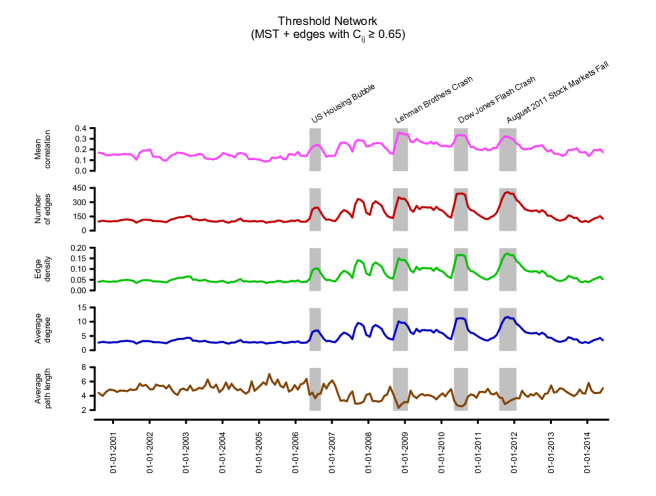
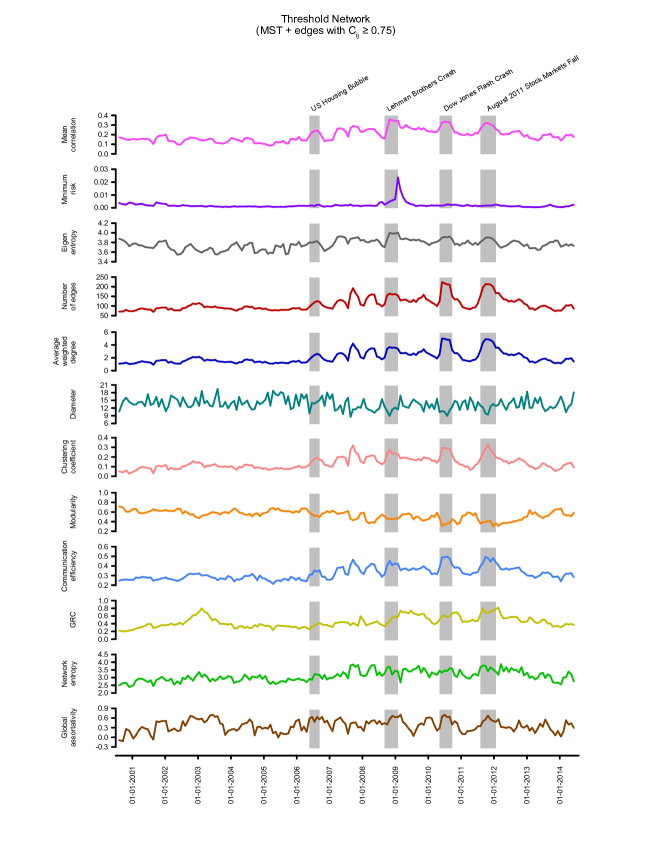
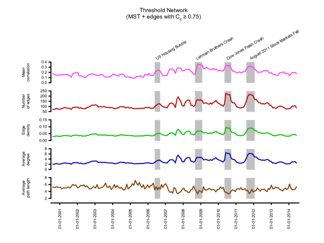
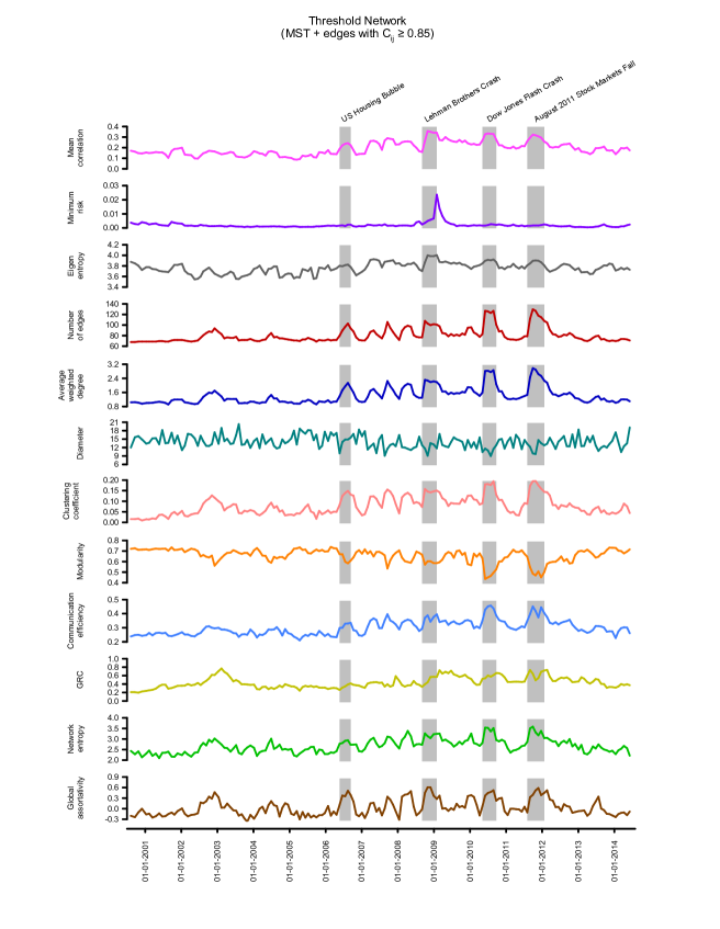
We reiterate that the threshold networks $\mathbf{S}^{\tau}(t)$ are constructed by computing the MST of the cross-correlation matrices $\mathbf{C}^{\tau}(t)$ followed by addition of edges with correlation $C_{ij}^{\tau}\geq 0.65$ (Methods). Intuitively, this network construction procedure ensures that each threshold network is a connected graph and captures the most relevant edges (correlations) between market indices. Since the obtained results may depend on the choice of the threshold ($0.65$) used for network construction, we present the temporal evolution of properties in networks constructed using $0.65$ as threshold in Main text, and in networks constructed using $0.75$ or $0.85$ as threshold in Supplementary Material. In the sequel, we will show that the qualitative nature of the obtained results are not very sensitive to the choice of $0.65$, $0.75$ or $0.85$ as thresholds to construct the networks of global market indices.

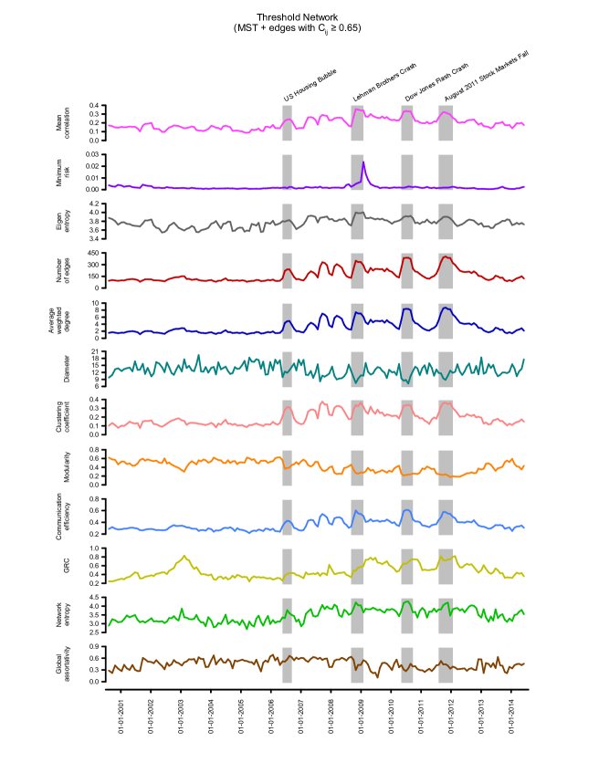
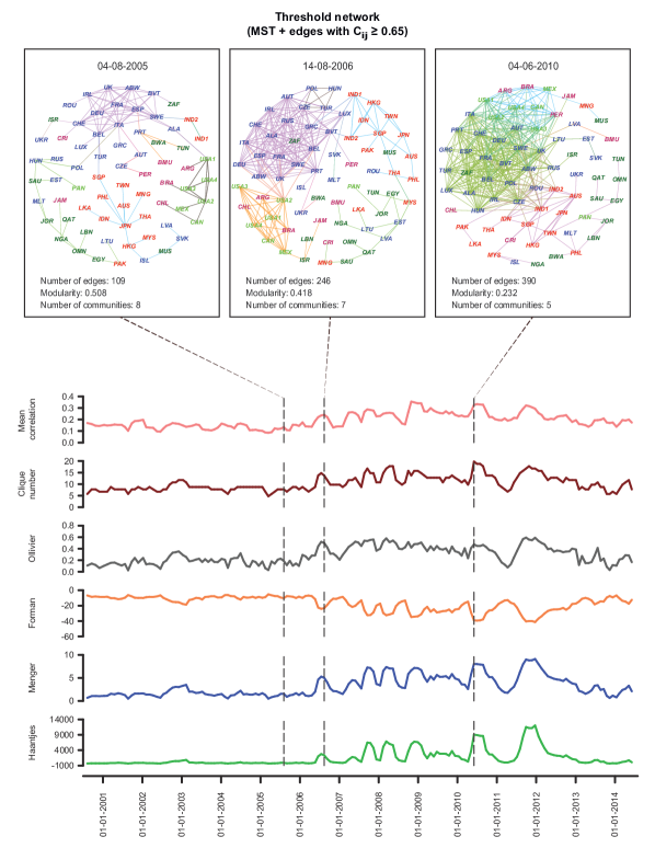
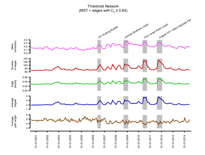
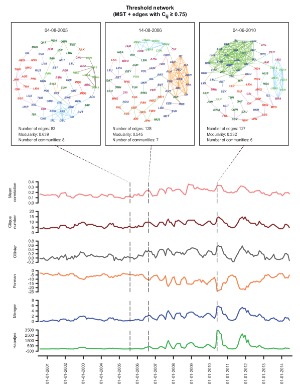
In Figures 1, 2 and Supplementary Figure S1, we show the temporal evolution of generic indicators and network measures in the threshold networks of global market indices over the 14-year period (2000-2014). Moreover, the four shaded regions in Figure 1 highlight four periods of financial crisis, namely, US housing bubble, Lehman brothers crash, Dow Jones flash crash, and August 2011 stock markets fall. From Figure 1, it is seen that the mean correlation between market indices increases during periods of financial crisis. Also, the eigen-entropy which is directly computed from the correlation matrix $\mathbf{C}^{\tau}(t)$ increases during crisis. Earlier works have shown that mean correlation and eigen-entropy are indicators of instabilities in stock market network Chakraborti et al. (2020a); Kukreti et al. (2020), and we show here that these measures can also serve as indicators of crisis in network of global financial indices. In Figure 1, we also show the temporal evolution of the minimum risk corresponding to the portfolio comprising the market indices using the Markowitz framework. Moving on to widely-used network properties, it is seen that the number of edges, edge density, average degree, average weighted degree, clustering coefficient, communication efficiency and network entropy increase while diameter, average shortest path length and modularity decrease during periods of financial crisis (Figure 1; Supplementary Figure S1). In Figure 1, we also show evolution of two other network measures, global reaching centrality (GRC) and global assortativity. In Figure 2, we also visualize the threshold network at three distinct time windows of $\tau=80$ days ending on trading days $t$ corresponding to 04-08-2005 (normal period), 14-08-2006 (US housing bubble crisis) and 04-06-2010 (Dow Jones flash crash) where the node colours are based on geographical regions of the market indices and edge colours are based on modules determined by Louvain method Blondel et al. (2008) for community detection. The identified communities in the three networks corresponding to normal period, US housing bubble and Dow Jones flash crash typically reflect the geographical proximity of financial market indices. For example, the indices of USA, Canada, Mexico, Argentina, Brazil and Chile form a single community in the threshold network for the normal period (Figure 2). It is evident that the number of edges in threshold networks correspoding to US housing bubble (246 edges) or Dow Jones flash crash (390 edges) are much higher in comparison to that for normal period (109 edges). In contrast, the modularity of threshold networks corresponding to the crisis periods, US housing bubble (0.418) or Dow Jones flash crash (0.232) are lower in comparison to that for normal period (0.508). In Figure 2, it is clearly seen that the clique number or size of the largest clique in threshold networks increases during financial crisis, and this is also evident from the network visualizations for normal period, US housing bubble and Dow Jones flash crash. Note that bubbles are not easy to detect. In fact, our proposition is that holistic approaches with network measures, both node- and edge-based measures, including geometric curvatures, may help us to better detect and distinguish the bubbles from market crashes, as also pointed out in recent contributions Chakraborti et al. (2020a); Samal et al. (2020). In sum, we find that during a normal period the network of global market indices is less connected, very modular and heterogeneous, whereas during a fragile period the network is highly connected, less modular and more homogeneous.

In addition to the node-centric global network measures described in the preceding paragraph, we have also studied edge-centric network measures, specifically, four discrete Ricci curvatures [Olivier-Ricci (OR), Forman-Ricci (OR), Menger-Ricci (MR) and Haantjes-Ricci (HR)] in threshold networks of global market indices. From Figure 2, it is seen that the average OR, MR or HR curvature of edges increase during crisis periods in comparison to normal periods. In contrast, the average FR curvature of edges decreases during crisis periods in comparison to normal periods. Notably, Sandhu et al. Sandhu et al. (2016) have shown that OR curvature can serve as indicator of fragility in stock market networks. However, to our knowledge, the present work is the first investigation of discrete Ricci curvatures in networks of global market indices. Note that different discretizations of Ricci curvature do not capture the entire features of the classical definition for continuous spaces, and thus, the four discrete Ricci curvatures studied here can capture different aspects of analyzed networks Samal et al. (2018). Overall, our results suggest that discrete Ricci curvatures can serve as indicators of fragility and monitor the health of the global financial system.

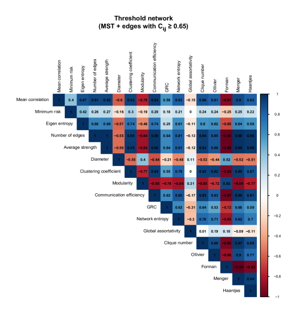
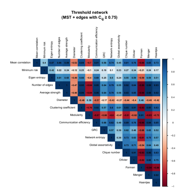
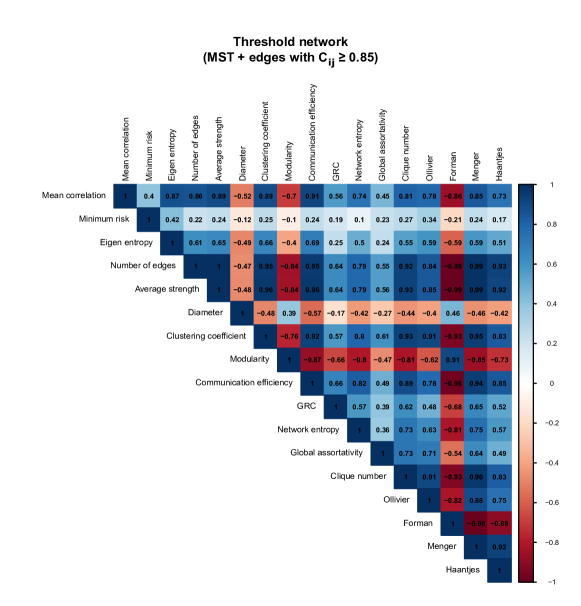
In Figure 3, we show the correlation between generic market indicators and different characteristics of the threshold networks $\mathbf{S}^{\tau}(t)$ of global market indices computed across the 14-year period from 2000 to 2014. From this figure, it is seen that eigen-entropy and several network measures have a very high (absolute) Pearson correlation ($\approx 0.9$) with generic indicator, mean correlation of market indices. Such network measures incude number of edges, average weighted degree (strength), clustering coefficient, communication efficiency, clique number, FR curvature and MR curvature. In contrast to mean correlation of market indices, there is moderate to no correlation between minimum risk corresponding to the portfolio comprising the market indices and eigen-entropy or network measures (Figure 3). In sum, these results indicate that network measures including edge-centric FR curvature can be used to forecast crisis and monitor the health of the global financial system. To the best of our knowledge, our work is the largest survey of network measures to identify potential network-centric indicators of fragility in global financial market indices.

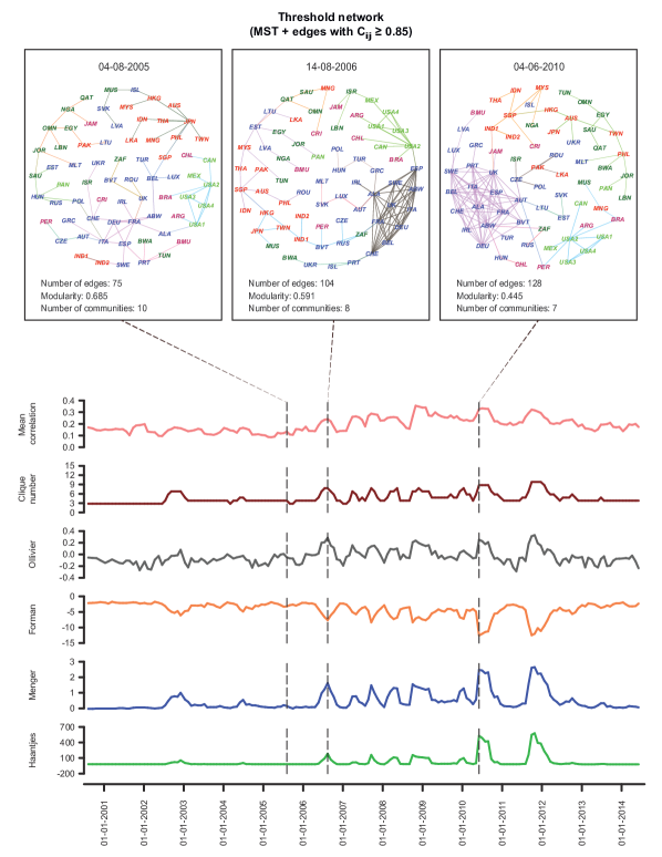
We must mention that though in the preceding paragraphs we have described only the results obtained from networks constructed using threshold of $0.65$, we have shown in Supplementary Figures S2-S9 that the qualitative conclusions remain unchanged even when networks with threshold of $0.75$ and $0.85$ are considered. In other words, our results are robust to the choice of threshold used to construct the networks of global market indices.

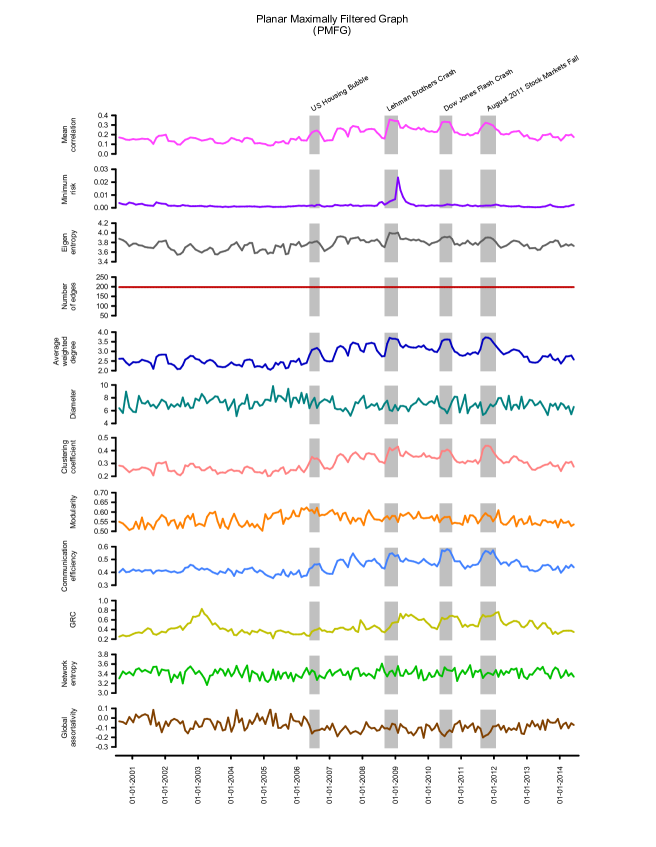
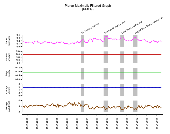
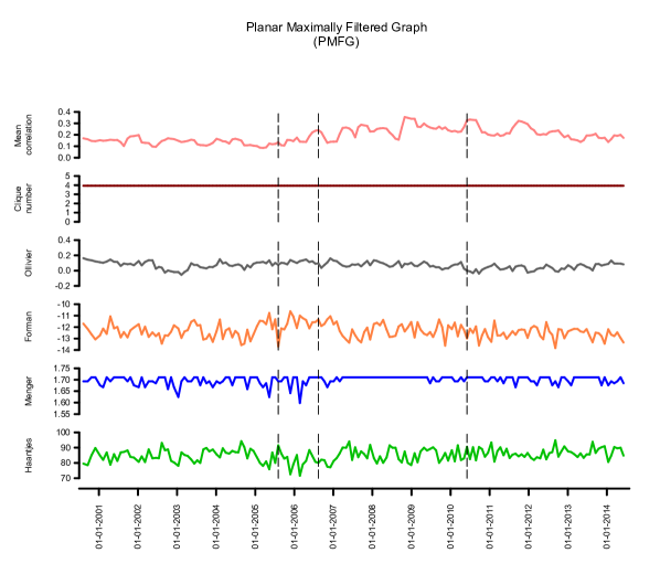
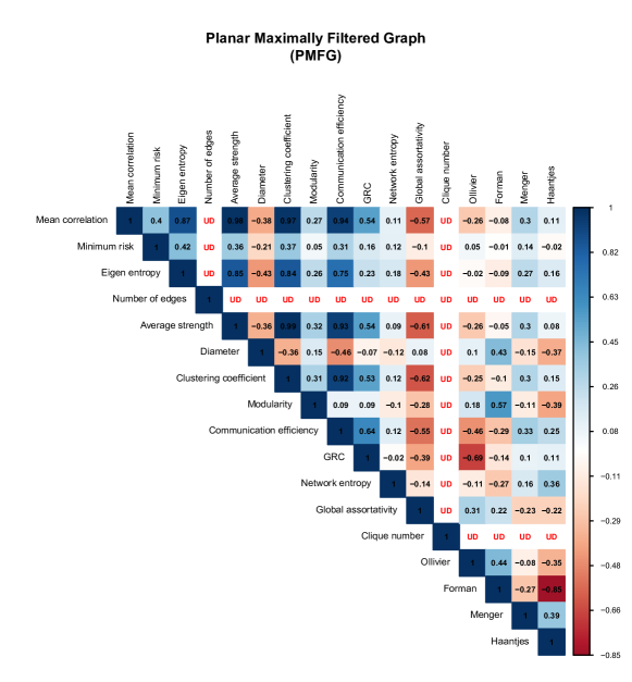
In previous works, the econophysics community has employed either minimum spanning tree (MST) Bonanno et al. (2000, 2003, 2004); Coelho et al. (2007); Eryiğit and Eryiğit (2009); Nobi et al. (2014); Junior et al. (2015); Wang and He (2017) or planar maximally fitered subgraph (PMFG) Eryiğit and Eryiğit (2009); Wang and He (2017) or threshold networks Kumar and Deo (2012); Nobi et al. (2014); Chen et al. (2020) to study the correlation structure between global financial market indices. As far as we know, this work is the first to use threshold networks of MST plus edges with correlation higher than a specified threshold, to study the temporal evolution of relationships between global financial market indices. In contrast, such threshold networks based on MST have been used earlier to study the structure of stock market networks Sandhu et al. (2016); Samal et al. (2020). While MST has a tree structure without loops or cycles, PMFG or threshold network permit loops or cycles. In Supplementary Text and Figures S10-S13, we also display the temporal evolution and correlation between generic market indicators and network measures in PMFG of global market indices constructed from cross-correlation matrices $\mathbf{C}^{\tau}(t)$. While the construction of PMFG unlike threshold networks is independent of any specific choice of the threshold, the number of edges (thus, edge density and average degree) is fixed in case of PMFG (Supplemetary Figures S10 and S11). Due to this reason, we find that most of the network measures studied here are not correlated with the generic market indicator, mean correlation of market indices, in PMFG case (Supplementary Figure S13). Still, we find that average weighted degree (strength), clustering coefficient and communication efficiency have very high correlation with mean correlation of market indices in PMFG based networks (Supplementary Figure S13). Based on these results, the threshold network construction based on MST plus edges with high correlation seems a better framework to monitor the state of the global financial system.

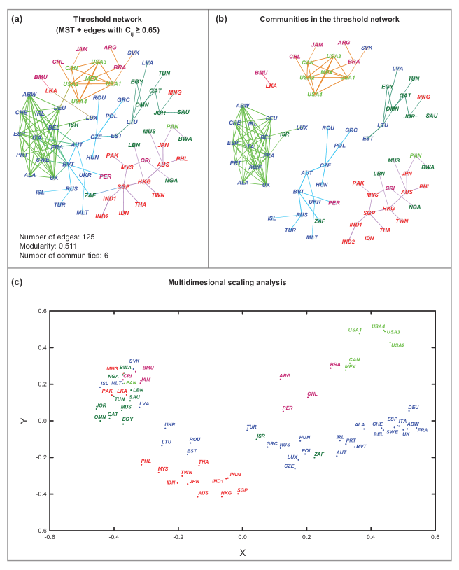
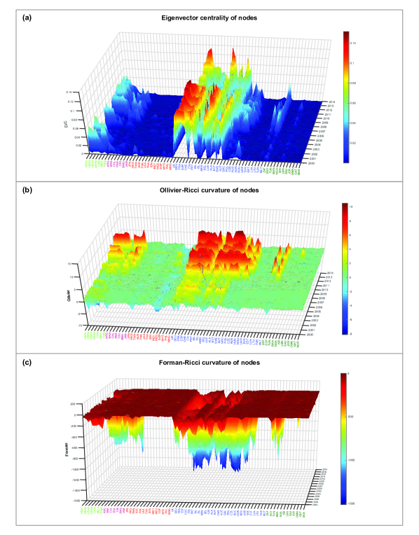
Finally, we have also studied the average correlation structure between global market indices over the 14-year period by computing the correlation matrix $\mathbf{C}^{T}$ between the 69 market indices by taking window size as the complete period of $T$ days between 2000 to 2014 (Methods). Subsequently, we have constructed a threshold network $\mathbf{S}^{T}$ corresponding to $\mathbf{C}^{T}$ by combining MST plus edges with correlation above the chosen threshold of $0.65$ (Methods). In Figure 4(a), we visualize this overall threshold network $\mathbf{S}^{T}$ of market indices for the complete 14-year period of $T$ days. In this figure, the node colours are based on geographical regions of the market indices and edge colours are based on communities obtained from Louvain method. In Figure 4(b), we have separated the communities in this overall threshold network $\mathbf{S}^{T}$ of market indices by removing the inter-module edges in the visualization. From Figure 4(a,b), it is clear that the market indices form communities in this overall threshold network based on their geographical proximity. Moreover, we have also employed multidimensional scaling (MDS) technique to map the 69 market indices into a $2$-dimensional space such that the distances between pairs of indices are preserved (Figure 4(c); Methods). It can be seen that the MDS map is able to partition the 69 market indices into groups based on their geographical proximity, and further, the structure in the MDS map has close resemblance to the community structure of the overall threshold network (Figure 4). For example, the grouping of indices from USA, Canada, Mexico, Argentina, Brazil and Chile can be seen in both the threshold network and MDS map (Figure 4). Interestingly, when we plotted in Supplementary Figure S14, the evolution of the eigenvector centralities of the nodes (market indices), as well as their OR and FR curvature, we found that there exist certain periods of time, when some of the countries in close geographical proximity display high (absolute) values and others display low values, indicative of the changes in the complex interactions and community structures.

4 Summary and concluding remarks

In summary, we have investigated the daily closing prices of 69 global financial indices over a 14-year period using various techniques of cross-correlations based network analysis. We have been able to continuously monitor the complex interactions among the global market indices by using a variety of network-centric measures, including, recently developed edge-centric discrete Ricci curvatures. In the present study of the global market indices, the novelty lies in: (i) Construction of the threshold network $\mathbf{S}^{\tau}(t)$, as superposition of the MST of the cross-correlation matrix and the network of edges with correlations $C_{ij}^{\tau}\geq 0.65$, which ensures that each threshold network is a connected graph and captures the most relevant edges (correlations) between market indices. In Supplementary Material, we have also reported the results for networks constructed using MST and two other threshold values, i.e., $C_{ij}^{\tau}\geq 0.75$ and $C_{ij}^{\tau}\geq 0.85$. Besides, we have also reported results for networks constructed using PMFG method. (ii) The usage of discrete Ricci curvatures in networks of global market indices, which capture the higher-order architecture of the complex financial system. To the best of our knowledge, this is the first study employing edge-based discrete Ricci curvatures to networks of global financial indices. Our recent work underscores the utility of edge-based curvature measures in analysis of networks of stocks Samal et al. (2020) or global financial indices. In future, curvature measures may also find application in other financial networks including Banking networks Namaki et al. (2020). (iii) The largest yet by no means exhaustive survey of network measures to identify potential network-centric indicators of fragility and systemic risk in the system of global financial market indices.

The global financial system has become increasingly complex and interdependent, and thus prone to sudden unpredictable changes like market crises. Our results, compared to the traditional market indicators, do provide a deeper understanding of the system of global financial markets. Specially, we find that the four discrete Ricci curvatures can be effectively used as indicators of fragility in global financial markets. We reiterate that the methods used in this work can detect instabilities in the market, and can be used as early warning signals so that policies can be made in order to prevent the occurrence of such events in the future.

Data Availability Statement

The codes used to construct the networks from correlation matrices and compute the different network measures are publicly available via the GitHub repository: https://github.com/asamallab/FinNetIndicators.

Author Contributions

A.S., S.K. and A.C. conceived the project. A.S., S.K., Y.Y. and A.C. performed the computations. S.K. compiled the dataset. Y.Y. and A.S. prepared the figures and tables. A.S. and A.C. analyzed the results. A.S., S.K., Y.Y. and A.C. wrote the manuscript. All authors have read and approved the manuscript.

Conflict of Interest

The authors declare that the research was conducted in the absence of any commercial or financial relationships that could be construed as a potential conflict of interest.

Supplementary Material

Supplementary Text

Markowitz portfolio optimization

We computed the risk corresponding to the portfolio comprising the market indices using the Markowitz framework as an indicator of the market risk for an investor who wishes to maximize the expected returns with the constraint of minimum variance. That is, the scheme minimizes $\mathrm{w}^{\prime}\Sigma\mathrm{w}-\phi R^{\prime}\mathrm{w}$ with respect to the normalized weight vector $\mathrm{w}$, where $\Sigma$ is the covariance matrix calculated from the logarithmic returns of the market indices, $\phi$ is the measure of risk appetite of investor and $R^{\prime}$ is the expected return of the market indices. We specify short-selling constraint, $\phi=0$ and $\mathrm{w}_{i}\geq 0$, such that we get a convex combination of returns of market indices for finding the minimum risk portfolio. These computations were performed using the in-built function in MATLAB Portfolio package (https://in.mathworks.com/help/finance/portfolio.html).

Standard network measures

Each network investigated in this work can be represented as a weighted and undirected graph $G(V,E)$ where $V$ is the set of vertices (or nodes) and $E$ is the set of edges (or links) in the graph. Also, an edge in a weighted graph has weight assigned to it, and this weight in real networks typically represents the distance or strength between vertices forming the edge. Depending on the network measure employed for characterizing the weighted graph, either the strength or the distance between two vertices could be the appropriate natural weight to use in the associated computation (Supplementary Table S2). Recall that while the strength represents similarity between two vertices, the distance reflects dissimilarity between them.

Here, we have studied weighted networks constructed from cross-correlation among global financial market indices (see Methods section in main text). For these networks of global market indices, we use the absolute value of the correlation $C_{ij}^{\tau}(t)$, that is $|C_{ij}^{\tau}(t)|$, between two market indices $i$ and $j$ as the strength of the edge between vertices $i$ and $j$ in the threshold network for epoch ending at $t$ for computations, and the ultrametric distance $D_{ij}^{\tau}(t)=\sqrt{2(1-C_{ij}^{\tau}(t))}$ as the distance of the edge between vertices $i$ and $j$ for computations (Supplementary Table S2). Note that the strength of an edge given by $|C_{ij}^{\tau}(t)|$ in the network of global financial market indices can take a value between 0 and 1, while the distance of an edge given by $D_{ij}^{\tau}(t)$ can take a value between 0 and 2.

In this work, we have characterized the structure of the global market indices network represented as a weighted and undirected graph using the following measures.

• The number of edges $m$ is given by $m=|E|$ and the number of vertices $n$ is given by $n=|V|$, where $|\ |$ denotes cardinality of the set.

• The number of edges incident on a given vertex gives its degree. The average degree of vertices can be expressed as $\langle k\rangle=\frac{2m}{n}$, where $n$ is the number of vertices and $m$ is the number of edges in graph $G$.

• The weighted degree (or strength) of a vertex is defined as the sum of weights of the edges incident on the vertex (Barrat et al., 2004). Consequently, the average weighted degree of vertices can be defined as $\langle k_{w}\rangle=\frac{2m_{w}}{n}$, where $m_{w}$ is the sum of weights assigned to all edges in graph $G$. We remark that the strength is the natural edge weight while computing the average weighted degree. In the main text, we also sometimes refer to average weighted degree as average strength.

• The edge density is defined as the ratio of the number of edges and the number of possible edges in graph $G$. Since a total of $\frac{n(n-1)}{2}$ edges are possible in an undirected graph $G$ ignoring self-edges, the edge density is given by $\frac{2m}{n(n-1)}$.

• The shortest path between any two vertices $i$ and $j$ in a graph is defined as a path wherein the sum of the distance along all the edges in the path is the minimum among all possible paths connecting the two vertices. The shortest path length, denoted by $d(i,j)$, is the sum of distances along edges in the shortest path between vertices $i$ and $j$ in the graph. The average (shortest) path length is an average of the shortest path lengths between every pair of vertices in the graph, that is,

  $$\langle L\rangle=\frac{1}{n(n-1)}\sum_{i\neq j\in V}d(i,j).$$ (2)

  We remark that distance is the natural edge weight while computing the average shortest path length in weighted graphs.

• The diameter of a graph is defined as the maximum of the shortest paths between all pairs of vertices, that is, $max\{d(i,j)\ \forall i,j\in V\}$.

• Communcation efficiency characterizes the global information flow or ability to exchange information in a network (Latora and Marchiori, 2001). The communication efficiency $\mu_{c}$ is defined as

  $$\mu_{c}=\frac{1}{n(n-1)}\sum_{i\neq j\in V}\frac{1}{d(i,j)}.$$ (3)

  We remark that distance is the natural edge weight while computing the communication efficiency in weighted graphs.

• The clustering coefficient of a vertex gives a measure of its tendency to form triads with its neighbouring vertices. Onnela Onnela et al. (2005) has proposed an approach to measure the clustering coefficient in weighted networks. For a vertex $i$ in weighted graph $G$, clustering coefficient is defined as

  $$C_{i}=\frac{2}{k_{i}(k_{i}-1)}\sum_{j,k}(a_{ij}a_{ik}a_{jk})^{1/3},$$ (4)

  where $j$ and $k$ are the neighbours of vertex $i$ and the summation runs over all such pairs of neighbours. The quantity in the summation is the intensity of the triangle attached to vertex $i$, and it takes the value $0$ if a triangle is not formed. The average clustering coefficent of a graph $G$ is the average of the clustering coefficients across all vertices in $G$. We remark that the strength is the natural edge weight while computing the clustering coefficient in weighted graphs.

• A network is said to exhibit community structure if it is possible to divide the vertices into distinct groups of densely connected vertices. Modularity measures edge density within a community in comparison to the edges between communities. Modularity of a weighted graph $G$ is defined as (Girvan and Newman, 2002; Blondel et al., 2008)

  $$Q=\frac{1}{2m_{w}}\sum_{i\neq j\in V}[\,a_{ij}-\frac{s_{i}s_{j}}{2m_{w}}]\delta(c_{i},c_{j})\,$$ (5)

  where $s_{i}$ and $s_{j}$ give the sum of weights of edges attached to vertices $i$ and $j$, respectively, $c_{i}$ and $c_{j}$ are the communities of $i$ and $j$, respectively, and $m_{w}$ is the sum of weights of all edges in $G$. We remark that the strength is the natural edge weight while computing the modularity in weighted graphs.

• Assortative mixing refers to the tendency of a vertex to attach to other vertices with similar properties in the network. A network is said to be assortative if high degree vertices tend to link with other high degree vertices. The assortativity coefficient was introduced by Newman (Newman, 2003) to measure degree correlations between vertices in an unweighted network. It is possible to extend this definition to weighted graphs by measuring how strongly any two vertices with similar degree tend to link with each other (Leung and Chau, 2007). The global assortativity of a weighted graph $G$ is defined as:

  $$r^{w}=\frac{\frac{1}{m_{w}}\sum_{e}a_{ij}k_{i}k_{j}-\left[\frac{1}{2m_{w}}\sum_{e}a_{ij}(k_{i}+k_{j})\right]^{2}}{\frac{1}{2m_{w}}\sum_{e}a_{ij}(k_{i}^{2}+k_{j}^{2})-\left[\frac{1}{2m_{w}}\sum_{e}a_{ij}(k_{i}+k_{j})\right]^{2}},$$ (6)

  where $m_{w}$ is the sum of weights of all edges, $k_{i}$ is the degree of the vertex $i$, $a_{ij}$ is the weight of edge between vertices $i$ and $j$, and the summation runs over all edges $e$ in weighted graph $G$. We remark that the strength is the natural edge weight while computing the global assortativity in weighted graphs.

• Measures for assortative mixing are limited since they quantify only the linear dependence. Network entropy was introduced to measure a network’s heterogeneity (Solé and Valverde, 2004), which follows a more general information-theoretic approach. The remaining (excess) degree of a vertex is defined as the number of edges leaving the vertex other than the one used to reach the vertex. The probability that a randomly chosen vertex has an excess degree $k$ is given by the remaining degree distribution $q_{k}=\frac{(k+1)p_{k+1}}{<k>}$. The network entropy $H(q)$ of a graph $G$ is then defined as

  $$H(q)=-\sum_{k}q_{k}log(q_{k}).$$ (7)

• The global reaching centrality (GRC) is a global network measure that aims to quantify hierarchy in complex networks (Mones et al., 2012). This measure can provide information on hierarchical organization in networks. GRC was introduced for unweighted and undirected graphs (Mones et al., 2012), and this measure can be extended to weighted graphs as follows. For an edge weighted graph $G$, we have

  $$GRC=\frac{\sum_{i\in V}\left[C^{max}-C(i))\right]}{n-1},$$ (8)

  where $C(i)$ is the local reaching centrality (LNC) (Mones et al., 2012) of vertex $i$, and $C^{max}$ is the maximum value of LNC across $n$ vertices in $G$. The LNC for a vertex $i$ in graph G is given by

  $$C(i)=\frac{1}{n-1}\sum_{j\in V\setminus\left\{i\right\}}\frac{1}{d(i,j)}.$$ (9)

  In the above equation, $d(i,j)$ is the previously defined shortest path length. The above equation is similar to the closeness centrality for weighted networks with disconnected components (Opsahl et al., 2010).

• The clique number is defined as the size of the maximal clique appearing in graph $G$. A clique $C$ in a graph $G(V,E)$ is a subset of the vertices, $C\subseteq V$, such that the induced subgraph is a complete graph.

• The centrality score of a vertex quantifies the relative importance of that vertex in the network. Degree centrality of a vertex, which is equal to its degree, is the simplest measure of centrality. Hence, a vertex can be considered important (or central) if it has a high degree. However, a vertex with low degree yet with edges to other important vertices is also an important vertex in the network, and this property can be accounted for by using the concept of eigenvector centrality. For a vertex $i$ in a weighted graph $G$, its eigenvector centrality $x_{i}$ is defined as the weighted sum of the centralities of its neighbours $i$ (Newman, 2004; Negre et al., 2018), that is

  $$x_{i}=\lambda^{-1}\sum_{j}a_{ij}x_{j}.$$ (10)

  The above equation can be rewritten as an eigenvector equation $\bf{Ax}=\lambda\bf{x}$, where $\bf{A}$ is the adjacency matrix of graph $G$, $\lambda$ is the largest eigenvalue of $\bf{A}$, and $\bf{x}$ is the eigenvector associated with $\lambda$. Thus, $x_{i}$ is the $i$^th component of the eigenvector $\bf{x}$.

Supplementary Table S2 gives an exhaustive list of network measures investigated here. In the table, we provide information on the type of edge weight, that is, strength or distance, used to compute each measure in the network of global market indices. The above-mentioned network measures were computed in networks of global market indices using programs written in python employing package NetworkX (Hagberg et al., 2008).

Edge-based curvature measures

The Ricci curvature in differential geometry is applicable to smooth manifolds (Jost, 2017). As the classical definition of Ricci curvature is not directly applicable to discrete objects including graphs or networks, multiple discrete notions of Ricci curvature have been proposed to date (Samal et al., 2018). While the classical definition of Ricci curvature is associated to vectors in smooth manifolds, in the case of discrete networks, the Ricci curvature is naturally associated to edges in the graph (Samal et al., 2018). Thus, the discrete Ricci curvatures are associated to edges rather than vertices or nodes in a graph. In other words, the discrete Ricci curvatures can be employed for edge-based analysis in contrast to commonly used measures such as degree and clustering coefficient which are suited for node-based analysis of networks (Sreejith et al., 2016; Samal et al., 2018).

Recall that the classical notion of Ricci curvature captures two essential geometric properties of the manifold, namely, volume growth and dispersion of geodesics. However, the discretizations of Ricci curvature which have been employed to characterize the structure of networks cannot capture the entire spectrum of geometric properties of the classical notion (Samal et al., 2018). Thus, different notions of discrete Ricci curvatures may capture different aspects of the structure of complex networks. In this section, we describe four notions of discrete Ricci curvature that we have used to study the networks of global market indices.

Ollivier-Ricci curvature

Ollivier (2007, 2009) has proposed a discrete notion of Ricci curvature which captures the volume growth property of the classical definition. Olivier’s proposal is based on the observation that in spaces of positive (negative) curvature, balls are closer (farther) to each other on the average than their centres. The Ollivier-Ricci curvature (OR) of an edge $e$ between vertices $i$ and $j$ in undirected graph $G$ is defined as

$$\mathbf{O}(e)=1-\frac{W_{1}(m_{i},m_{j})}{d(i,j)}\ ,$$ (11)

where $m_{i}$ and $m_{j}$ are discrete probability measures assigned to vertices $i$ and $j$, respectively, $d(i,j)$ is the distance between $i$ and $j$, as defined in the previous section, and $W_{1}$ denotes the Wasserstein distance (Vaserstein, 1969), which is the transportation distance between $m_{i}$ and $m_{j}$, given by

$$W_{1}(m_{i},m_{j})=\inf_{\mu_{i,j}\in\prod(m_{i},m_{j})}\sum_{(i^{\prime},j^{\prime})\in V\times V}d(i^{\prime},j^{\prime})\mu_{i,j}(i^{\prime},j^{\prime}),$$ (12)

where $\prod(m_{i},m_{j})$ is the set of probability measures $\mu_{i,j}$ that satisfy

$$\sum_{j^{\prime}\in V}\mu_{i,j}(i^{\prime},j^{\prime})=m_{i}(i^{\prime}),\,\,\sum_{i^{\prime}\in V}\mu_{i,j}(i^{\prime},j^{\prime})=m_{j}(j^{\prime}).$$ (13)

The probability distribution $m_{i}$ is taken to be uniform over the the neighbouring vertices of $i$ (Lin et al., 2011). We have computed the average OR curvature of edges in networks of global market indices in this work. While computing the OR curvature in networks of global market indices, the weight of each edge is taken to be the distance. Given the OR curvature of edges in the graph, it is straightforward to define the OR curvature of a vertex $v$ as

$$\mathbf{O}(v)=\sum_{e\ \sim\ v}\mathbf{O}(e)\,$$ (14)

where $e\sim v$ is the set of edges $e$ incident on vertex $v$. The above definition of OR curvature of a vertex is analogous to scalar curvature in Riemannian geometry (Samal et al., 2018).

Forman-Ricci curvature

Forman’s discretization (Forman, 2003) captures the geodesic dispersal property of the classical notion of Ricci curvature (Sreejith et al., 2016). It is based on the relation between the Riemann-Laplace operator and Ricci curvature. Recently, Forman-Ricci curvature (FR) was adapted for the analysis of unweighted and weighted networks (Sreejith et al., 2016, 2017). Intuitively, FR curvature quantifies the information spread at the ends of an edge in the network. High negative FR value for an edge indicates more spread of information at its ends. For an edge $e$ between vertices $i$ and $j$ in an undirected graph $G$, FR is defined as

$$\mathbf{F}(e)=w_{e}\left(\frac{w_{i}}{w_{e}}+\frac{w_{j}}{w_{e}}-\sum_{e_{i}\ \sim\ e,\ e_{j}\ \sim\ e}\left[\frac{w_{i}}{\sqrt{w_{e}w_{e_{j}}}}+\frac{w_{j}}{\sqrt{w_{e}w_{e_{j}}}}\right]\right)\,$$ (15)

where $w_{e}$ denotes the weight of the edge $e$, $w_{i}$ and $w_{j}$ denote the weights associated with the vertices $i$ and $j$, respectively, $e_{i}\sim e$ and $e_{j}\sim e$ denote the set of edges incident on vertices $i$ and $j$, respectively, after excluding the edge $e$. We have computed the average FR curvature of edges in networks of global market indices in this work. While computing the FR curvature in networks of global market indices, the weight of each edge is taken to be the distance while the weight of each vertex is taken to be $1$.

Given the FR curvature of edges in the graph, it is straightforward to define the FR curvature of a vertex $v$ as

$$\mathbf{F}(v)=\sum_{e\ \sim\ v}\mathbf{F}(e)\,$$ (16)

where $e\sim v$ is the set of edges $e$ incident on vertex $v$. The above definition of FR curvature of a vertex is analogous to scalar curvature in Riemannian geometry (Sreejith et al., 2017).

Menger-Ricci curvature

Menger defined the curvature of a metric triangle $T$ (Menger, 1930) formed by three points in space as the reciprocal $\frac{1}{R(T)}$ of the radius $R(T)$ of the circumcircle of that triangle. Given a triangle $T=T(a,b,c)$ with sides $a,\ b,\ c$ in a metric space $(M,d)$, the Menger curvature of $T$ is given by

$$K_{M}(T)=\frac{\sqrt{p(p-a)(p-b)(p-c)}}{a\cdot b\cdot c}\,$$ (17)

where $p=(a+b+c)/2$. It is possible to extend the above definition to unweighted and undirected networks (Saucan et al., 2019b, 2020), where one considers combinatorial triangles with length of each side equal to $1$, and this gives $K_{M}(T)=\sqrt{3}/2$. Then the Menger-Ricci curvature (MR) of an edge $e$ in the graph $G$ can be defined as

$$\kappa_{M}(e)=\sum_{T_{e}\sim e}\kappa_{M}(T_{e})\,,$$ (18)

where $T_{e}\sim e$ denote the triangles adjacent to the edge $e$. An edge will have high positive value of MR curvature if it is part of many triangles in the network. In this work, we have computed the average MR curvature of edges in networks of global market indices.

Haantjes-Ricci curvature

Haantjes (Haantjes, 1947) defined the curvature of a metric curve as the ratio of the length of the arc of the curve and that of the chord it subtends. More precisely, given three points $p$, $q$ and $r$ on a curve in a metric space such that $p$ lies between $q$ and $r$, the Haantjes curvature at the point $p$ is defined as

$$\kappa_{H}^{2}(p)=24\lim_{q,r\rightarrow p}\frac{l(\widehat{qr})-d(q,r)}{\big{(}d(q,r)\big{)}^{3}}\,,$$ (19)

where $l(\widehat{qr})$ denotes the length of the arc $\widehat{qr}$. The above definition can be extended to networks by replacing the arc $\widehat{qr}$ with a path between the two vertices and the subtending chord by the edge between the two vertices (Saucan et al., 2019b, 2020). Given a simple path $\pi=i,\ldots,j$ between the two vertices $i$ and $j$ connected by an edge $e$ in the unweighted graph $G$, the Haantjes curvature of the path takes the value

$$\kappa_{H}(\pi)=\sqrt{n-1}\ ,$$ (20)

where $n$ is the number of edges appearing in the path $\pi$. Then the Haantjes-Ricci curvature (HR) of the edge $e$ can be defined as (Saucan et al., 2019b, 2020)

$$\kappa_{H}(e)=\sum_{\pi\sim e}\kappa_{H}(\pi)\,,$$ (21)

where the summation runs over all the paths between vertices $i$ and $j$. In this work, we have computed the average HR curvature of edges in networks of global market indices by ignoring edge weights. Further, computational constraints permitted only consideration of paths $\pi$ of length $\leq 5$ between two vertices at the ends of any edge while computing the HR curvature in networks of global market indices.

Planar maximally filtered graph (PMFG) construction and characteristics

Here, we describe an alternate network construction framework, namely, the planar maximally filtered graph (PMFG) (Tumminello et al., 2005), which has been widely-used to study the relationship between global financial market indices. Briefly, the PMFG $\mathbf{P}^{\tau}(t)$ of market indices can be constructed for the time-series of cross-correlation matrices $\mathbf{C}^{\tau}(t)$ of window size $\tau=80$ days and an overlapping shift of $\Delta\tau=20$ days over the 14-year period as follows (see Methods section in main text for the computation of cross-correlation matrices $\mathbf{C}^{\tau}(t)$ starting from the logarithmic returns of daily closing prices of 69 global market indices). Firstly, a sorted list of edges is created based on the decreasing order of correlation in the matrix $\mathbf{C}^{\tau}(t)$. Next, each edge in the sorted list is considered for inclusion in the PMFG based on the decreasing order of correlation. An edge between vertices $i$ and $j$ is added to PMFG, if and only if the resulting graph can be embedded on a sphere, i.e., it is a planar graph. Following this scheme, the final network obtained is a PMFG with $3(N-1)$ edges where $N$ is the number of vertices in the graph. Note that the minimum spanning tree (MST) in contrast to PMFG contains $N-1$ edges, and it has no loops or cliques. Importantly, in addition to the hierarchical organization of the MST, the PMFG also includes information on the loops and cliques involving upto four vertices present in the correlation matrix. We remark that PMFG is a special case of a more general method of network construction (Tumminello et al., 2005), wherein the edges are added under the topological constraint that the resulting graph can be embedded on a surface of genus $g=k$ where $k$ is a postive integer. In case of PMFG, the graph is embedded on a surface of genus $g=0$ which is a sphere.

In Supplementary Figures S10-S13, we show the temporal evolution and correlation between generic market indicators and network measures in PMFG $\mathbf{P}^{\tau}(t)$ of market indices constructed from cross-correlation matrices $\mathbf{C}^{\tau}(t)$ as described above.

Figure S1: Evolution of generic indicators and network characteristics for the global market indices networks $\mathbf{S}^{\tau}(t)$, constructed from the correlation matrices $\mathbf{C}^{\tau}(t)$ of window size $\tau=80$ days and an overlapping shift of $\Delta\tau=20$ days over a period of 14 years (2000-2014). The threshold networks $\mathbf{S}^{\tau}(t)$ were constructed by adding edges with correlation $C_{ij}^{\tau}(t)\geq 0.65$ to the minimum spanning tree (MST). From top to bottom, we compare the plot of mean correlation among market indices, number of edges, edge density, average degree and average path length. The four shaded regions correspond to the epochs around the four important market events, namely, US housing bubble, Lehman brothers crash, Dow Jones flash crash, and August 2011 stock markets fall.

Figure S2: Evolution of generic indicators and network characteristics for the global market indices networks $\mathbf{S}^{\tau}(t)$, constructed from the correlation matrices $\mathbf{C}^{\tau}(t)$ of window size $\tau=80$ days and an overlapping shift of $\Delta\tau=20$ days over a period of 14 years (2000-2014). The threshold networks $\mathbf{S}^{\tau}(t)$ were constructed by adding edges with correlation $C_{ij}^{\tau}(t)\geq 0.75$ to the minimum spanning tree (MST). From top to bottom, we compare the plot of mean correlation among market indices, minimum risk corresponding to the Markowitz portfolio optimization, eigen-entropy, number of edges, average weighted degree, diameter, clustering coefficient, modularity, communication efficiency, global reaching centrality (GRC), network entropy and global assortativity. The four shaded regions correspond to the epochs around the four important market events, namely, US housing bubble, Lehman brothers crash, Dow Jones flash crash, and August 2011 stock markets fall.

Figure S3: Evolution of generic indicators and network characteristics for the global market indices networks $\mathbf{S}^{\tau}(t)$, constructed from the correlation matrices $\mathbf{C}^{\tau}(t)$ of window size $\tau=80$ days and an overlapping shift of $\Delta\tau=20$ days over a period of 14 years (2000-2014). The threshold networks $\mathbf{S}^{\tau}(t)$ were constructed by adding edges with correlation $C_{ij}^{\tau}(t)\geq 0.75$ to the minimum spanning tree (MST). From top to bottom, we compare the plot of mean correlation among market indices, number of edges, edge density, average degree and average path length. The four shaded regions correspond to the epochs around the four important market events, namely, US housing bubble, Lehman brothers crash, Dow Jones flash crash, and August 2011 stock markets fall.

Figure S4: Evolution of generic indicators and network characteristics for the global market indices networks $\mathbf{S}^{\tau}(t)$, constructed from the correlation matrices $\mathbf{C}^{\tau}(t)$ of window size $\tau=80$ days and an overlapping shift of $\Delta\tau=20$ days over a period of 14 years (2000-2014). The threshold networks $\mathbf{S}^{\tau}(t)$ were constructed by adding edges with correlation $C_{ij}^{\tau}(t)\geq 0.85$ to the minimum spanning tree (MST). From top to bottom, we compare the plot of mean correlation among market indices, minimum risk corresponding to the Markowitz portfolio optimization, eigen-entropy, number of edges, average weighted degree, diameter, clustering coefficient, modularity, communication efficiency, global reaching centrality (GRC), network entropy and global assortativity. The four shaded regions correspond to the epochs around the four important market events, namely, US housing bubble, Lehman brothers crash, Dow Jones flash crash, and August 2011 stock markets fall.

Figure S5: Evolution of generic indicators and network characteristics for the global market indices networks $\mathbf{S}^{\tau}(t)$, constructed from the correlation matrices $\mathbf{C}^{\tau}(t)$ of window size $\tau=80$ days and an overlapping shift of $\Delta\tau=20$ days over a period of 14 years (2000-2014). The threshold networks $\mathbf{S}^{\tau}(t)$ were constructed by adding edges with correlation $C_{ij}^{\tau}(t)\geq 0.85$ to the minimum spanning tree (MST). From top to bottom, we compare the plot of mean correlation among market indices, number of edges, edge density, average degree and average path length. The four shaded regions correspond to the epochs around the four important market events, namely, US housing bubble, Lehman brothers crash, Dow Jones flash crash, and August 2011 stock markets fall.

Figure S6: Evolution of network characteristics and visualization of the threshold networks $\mathbf{S}^{\tau}(t)$ of market indices with window size $\tau=80$ days and an overlapping shift of $\Delta\tau=20$ days, constructed by adding edges with correlation $C_{ij}^{\tau}(t)\geq 0.75$ to the MST. (Lower panel) Comparison of the plots of mean correlation among market indices, clique number, average of Ollivier-Ricci (OR), Forman-Ricci (FR), Menger-Ricci (MR), and Haantjes-Ricci (HR) curvature of edges in threshold networks over the 14-year period. (Upper panel) Visualization of the threshold networks at three distinct epochs of $\tau=80$ days ending on trading days $t$ equal to 04-08-2005 (normal), 14-08-2006 (US housing bubble) and 04-06-2010 (Dow Jones flash crash). Threshold networks show higher number of edges and lower number of communities during crisis. Correspondingly, there is an increase in mean correlation, clique number, average OR, MR and HR curvature, and decrease in average FR curvature of threshold networks during financial crisis. Node colours and labels are based on geographical region and country, respectively, of the indices and edge colours are based on the community determined by Louvain method. The four USA market indices, NASDAQ, NYSE, RUSSELL1000 and SPX, are labelled as USA1, USA2, USA3 and USA4, respectively, while the two Indian indices, NIFTY and SENSEX30, are labelled as IND1 and IND2, respectively.

Figure S7: Evolution of network characteristics and visualization of the threshold networks $\mathbf{S}^{\tau}(t)$ of market indices with window size $\tau=80$ days and an overlapping shift of $\Delta\tau=20$ days, constructed by adding edges with correlation $C_{ij}^{\tau}(t)\geq 0.85$ to the MST. (Lower panel) Comparison of the plots of mean correlation among market indices, clique number, average of Ollivier-Ricci (OR), Forman-Ricci (FR), Menger-Ricci (MR), and Haantjes-Ricci (HR) curvature of edges in threshold networks over the 14-year period. (Upper panel) Visualization of the threshold networks at three distinct epochs of $\tau=80$ days ending on trading days $t$ equal to 04-08-2005 (normal), 14-08-2006 (US housing bubble) and 04-06-2010 (Dow Jones flash crash). Threshold networks show higher number of edges and lower number of communities during crisis. Correspondingly, there is an increase in mean correlation, clique number, average OR, MR and HR curvature, and decrease in average FR curvature of threshold networks during financial crisis. Node colours and labels are based on geographical region and country, respectively, of the indices and edge colours are based on the community determined by Louvain method. The four USA market indices, NASDAQ, NYSE, RUSSELL1000 and SPX, are labelled as USA1, USA2, USA3 and USA4, respectively, while the two Indian indices, NIFTY and SENSEX30, are labelled as IND1 and IND2, respectively.

Figure S8: Correlation between generic indicators and network characteristics of the global market indices networks $\mathbf{S}^{\tau}(t)$, constructed from the correlation matrices $\mathbf{C}^{\tau}(t)$ of window size $\tau=80$ days and an overlapping shift of $\Delta\tau=20$ days over a period of 14 years (2000-2014). The threshold networks $\mathbf{S}^{\tau}(t)$ were constructed by adding edges with correlation $C_{ij}^{\tau}(t)\geq 0.75$ to the minimum spanning tree (MST).

Figure S9: Correlation between generic indicators and network characteristics of the global market indices networks $\mathbf{S}^{\tau}(t)$, constructed from the correlation matrices $\mathbf{C}^{\tau}(t)$ of window size $\tau=80$ days and an overlapping shift of $\Delta\tau=20$ days over a period of 14 years (2000-2014). The threshold networks $\mathbf{S}^{\tau}(t)$ were constructed by adding edges with correlation $C_{ij}^{\tau}(t)\geq 0.85$ to the minimum spanning tree (MST).

Figure S10: Evolution of generic indicators and network characteristics for PMFG $\mathbf{P}^{\tau}(t)$ of global market indices, constructed from the correlation matrices $\mathbf{C}^{\tau}(t)$ of window size $\tau=80$ days and an overlapping shift of $\Delta\tau=20$ days over a period of 14 years (2000-2014). From top to bottom, we compare the plot of mean correlation among market indices, minimum risk corresponding to the Markowitz portfolio optimization, eigen-entropy, number of edges, average weighted degree, diameter, clustering coefficient, modularity, communication efficiency, global reaching centrality (GRC), network entropy and global assortativity. The four shaded regions correspond to the epochs around the four important market events, namely, US housing bubble, Lehman brothers crash, Dow Jones flash crash, and August 2011 stock markets fall.

Figure S11: Evolution of generic indicators and network characteristics for PMFG $\mathbf{P}^{\tau}(t)$ of global market indices, constructed from the correlation matrices $\mathbf{C}^{\tau}(t)$ of window size $\tau=80$ days and an overlapping shift of $\Delta\tau=20$ days over a period of 14 years (2000-2014). From top to bottom, we compare the plot of mean correlation among market indices, number of edges, edge density, average degree and average path length. The four shaded regions correspond to the epochs around the four important market events, namely, US housing bubble, Lehman brothers crash, Dow Jones flash crash, and August 2011 stock markets fall.

Figure S12: Evolution of network characteristics for PMFG $\mathbf{P}^{\tau}(t)$ of global market indices with window size $\tau=80$ days and an overlapping shift of $\Delta\tau=20$ days. Comparison of the plots of mean correlation among market indices, clique number, average of Ollivier-Ricci (OR), Forman-Ricci (FR), Menger-Ricci (MR), and Haantjes-Ricci (HR) curvature of edges in PMFG over the 14-year period.

Figure S13: Correlation between generic indicators and network characteristics for PMFG $\mathbf{P}^{\tau}(t)$ of global market indices, constructed from the correlation matrices $\mathbf{C}^{\tau}(t)$ of window size $\tau=80$ days and an overlapping shift of $\Delta\tau=20$ days over a period of 14 years (2000-2014). For some pairs of measures investigated here, the correlation cannot be computed as at least one of the measures has zero variance, and thus, we specify undefined (‘UD’) for correlation between such pairs of measures in this plot.

Figure S14: Three dimensional plot showing the evolution of (a) normalized eigenvector centrality, (b) Ollivier-Ricci (OR) curvature, and (c) Forman-Ricci (FR) curvature for each of the 69 market indices (nodes) across the time-series of 172 threshold networks $\mathbf{S}^{\tau}(t)$ of market indices computed with window size $\tau=80$ days and an overlapping shift of $\Delta\tau=20$ days, constructed by adding edges with correlation $C_{ij}^{\tau}(t)\geq 0.65$ to the MST. We compute the OR and FR curvature of nodes in the threshold networks based on the OR and FR curvature of incident edges on each node. Here, the colours of the market indices are based on geographical region of their country. The four USA market indices, NASDAQ, NYSE, RUSSELL1000 and SPX, are labelled as USA1, USA2, USA3 and USA4, respectively, while the two Indian indices, NIFTY and SENSEX30, are labelled as IND1 and IND2, respectively. It can be seen that there exist certain periods of time, when some of the market indices in close geographical proximity display high (absolute) values while others display low values, indicative of the changes in the complex interactions and community structures in global financial network.

Table S1: List of 69 global financial market indices across 65 countries considered in this work. For each financial market index, the table lists the country of origin, country code, index code, region code and geographical region. This dataset was obtained from Bloomberg.

S. No.	Country	Country code	Index code	Region code	Region
1	United States of America	USA	NASDAQ COMPOSITE	NA	North America
2	United States of America	USA	NYSE COMPOSITE	NA	North America
3	United States of America	USA	RUSSELL 1000	NA	North America
4	United States of America	USA	SPX	NA	North America
5	Canada	CAN	SPTSX	NA	North America
6	Mexico	MEX	MEXBOL	NA	North America
7	Panama	PAN	BVPSBVPS	NA	North America
8	Argentina	ARG	MERVAL	SA	South America
9	Brazil	BRA	IBOV	SA	South America
10	Chile	CHL	IPSA	SA	South America
11	Peru	PER	IGBVL	SA	South America
12	Costa Rica	CRI	BCT	SA	South America
13	Bermuda	BMU	BSX	SA	South America
14	Jamaica	JAM	JMSMX	SA	South America
15	Japan	JPN	TPX	AP	Asia Pacific
16	Hang Kong	HKG	Hang Seng	AP	Asia Pacific
17	Taiwan	TWN	TWSE	AP	Asia Pacific
18	Australia	AUS	AS51	AP	Asia Pacific
19	Pakistan	PAK	KSE100	AP	Asia Pacific
20	Sri Lanka	LKA	CSEALL	AP	Asia Pacific
21	Thailand	THA	SET	AP	Asia Pacific
22	Indonesia	IDN	JCI	AP	Asia Pacific
23	India	IND	NIFTY	AP	Asia Pacific
24	India	IND	SENSEX30	AP	Asia Pacific
25	Singapore	SGP	FSSTI	AP	Asia Pacific
26	Malaysia	MYS	FBMKLCI	AP	Asia Pacific
27	Philippines	PHL	PCOMP	AP	Asia Pacific
28	Mongolia	MNG	MSETOP	AP	Asia Pacific
29	United Kingdom	UK	UKX	EME	Europe Middle East
30	Germany	DEU	DAX	EME	Europe Middle East
31	France	FRA	CAC40	EME	Europe Middle East
32	Spain	ESP	IBEX35	EME	Europe Middle East
33	Switzerland	CHE	SMI	EME	Europe Middle East
34	Italy	ITA	FTSEMIB	EME	Europe Middle East
35	Portugal	PRT	BVLX	EME	Europe Middle East
36	Ireland	IRL	ISEQ	EME	Europe Middle East
37	Iceland	ISL	ICEXI	EME	Europe Middle East
38	Netherlands	ABW	AEX	EME	Europe Middle East
39	Belgium	BEL	BEL20	EME	Europe Middle East
40	Luxembourg	LUX	LUXXX	EME	Europe Middle East
41	Finland	ALA	HEX	EME	Europe Middle East
42	Norway	BVT	OBX	EME	Europe Middle East
43	Sweden	SWE	OMX	EME	Europe Middle East
44	Austria	AUT	ATX	EME	Europe Middle East
45	Greece	GRC	ASE	EME	Europe Middle East
46	Poland	POL	WIG	EME	Europe Middle East
47	Czech Republic	CZE	PX	EME	Europe Middle East
48	Russia	RUS	MICEX	EME	Europe Middle East
49	Hungary	HUN	BUX	EME	Europe Middle East
50	Romania	ROU	BET	EME	Europe Middle East

51	Ukraine	UKR	PFTS	EME	Europe Middle East
52	Slovakia	SVK	SKSM	EME	Europe Middle East
53	Estonia	EST	TALSE	EME	Europe Middle East
54	Lativa	LVA	RIGSE	EME	Europe Middle East
55	Lithuania	LTU	VILSE	EME	Europe Middle East
56	Turkey	TUR	XU100	EME	Europe Middle East
57	Malta	MLT	MALTEX	EME	Europe Middle East
58	South Africa	ZAF	JALSH	AME	Africa/Middle East
59	Egypt	EGY	HERMES	AME	Africa/Middle East
60	Tunisia	TUN	TUSISE	AME	Africa/Middle East
61	Botswana	BWA	BGSMDC	AME	Africa/Middle East
62	Nigeria	NGA	NGSEINDX	AME	Africa/Middle East
63	Israel	ISR	TA-25	AME	Africa/Middle East
64	Lebanon	LBN	BLOM	AME	Africa/Middle East
65	Saudi Arabia	SAU	SASEIDX	AME	Africa/Middle East
66	Jordan	JOR	JOSMGNFF	AME	Africa/Middle East
67	Oman	OMN	MSM30	AME	Africa/Middle East
68	Qatar	QAT	DSM	AME	Africa/Middle East
69	Mauritius	MUS	SEMDEX	AME	Africa/Middle East

Table S2: Classification of network measures employed to characterize the networks of global market indices into those for unweighted or weighted graphs. For each measure evaluated in the weighted graph, we list the appropriate natural weight, strength or distance, which is used in the associated computation.

S. No.	Measure	Type of measure	Type of weight
1	Number of edges	Unweighted	-
2	Average degree	Unweighted	-
3	Edge density	Unweighted	-
4	Clique number	Unweighted	-
5	Network entropy	Unweighted	-
6	Average weighted degree	Weighted	Strength
7	Global assortativity	Weighted	Strength
8	Clustering coefficient	Weighted	Strength
9	Modularity	Weighted	Strength
10	Eigenvector centrality	Weighted	Strength
11	Average shortest path length	Weighted	Distance
12	Diameter	Weighted	Distance
13	Global reaching centrality	Weighted	Distance
14	Communication efficiency	Weighted	Distance
15	Ollivier-Ricci curvature	Weighted	Distance
16	Forman-Ricci curvature	Weighted	Distance
17	Menger-Ricci curvature	Unweighted	-
18	Haantjes-Ricci curvature	Unweighted	-

References

- Mantegna (1999a) R. N. Mantegna, Computer Physics Communications 121-122, 153 (1999a).
- Mantegna (1999b) R. N. Mantegna, The European Physical Journal B 11, 193 (1999b).
- Onnela et al. (2003a) J.-P. Onnela, A. Chakraborti, K. Kaski, J. Kertsz, and A. Kanto, Physica Scripta T106, 48 (2003a).
- Onnela et al. (2004) J.-P. Onnela, K. Kaski, and J. Kertész, European Physical Journal B 38, 353 (2004).
- Boginski et al. (2005) V. Boginski, S. Butenko, and P. M. Pardalos, Computational Statistics & Data Analysis 48, 431 (2005).
- Tumminello et al. (2005) M. Tumminello, T. Aste, T. Di Matteo, and R. N. Mantegna, Proceedings of the National Academy of Sciences USA 102, 10421 (2005).
- Bonanno et al. (2003) G. Bonanno, G. Caldarelli, F. Lillo, and R. N. Mantegna, Physical Review E 68, 046130 (2003).
- Onnela et al. (2003b) J.-P. Onnela, A. Chakraborti, K. Kaski, J. Kertesz, and A. Kanto, Physical Review E 68, 056110 (2003b).
- Bonanno et al. (2004) G. Bonanno, G. Caldarelli, F. Lillo, S. Micciché, N. Vandewalle, and R. N. Mantegna, European Physical Journal B 38, 363 (2004).
- Bonanno et al. (2000) G. Bonanno, N. Vandewalle, and R. N. Mantegna, Physical Review E 62, R7615 (2000).
- Nobi et al. (2014) A. Nobi, S. Lee, D. H. Kim, and J. W. Lee, Physics Letters A 378, 2482 (2014).
- Wang and He (2017) J. Wang and J. He, in 2017 17th International Conference on Control, Automation and Systems (ICCAS) (2017) pp. 498–504.
- Coelho et al. (2007) R. Coelho, C. G. Gilmore, B. Lucey, P. Richmond, and S. Hutzler, Physica A 376, 455 (2007).
- Kumar and Deo (2012) S. Kumar and N. Deo, Physical Review E 86, 026101 (2012).
- Junior et al. (2015) L. Junior, A. Mullokandov, and D. Kenett, Journal of Risk and Financial Management 8, 227 (2015).
- Lee and Nobi (2018) J. W. Lee and A. Nobi, Computational Economics 51, 195 (2018).
- León et al. (2017) C. León, G. Kim, C. Martínez, and D. Lee, Quantitative Finance 17, 1 (2017).
- Saeedian et al. (2019) M. Saeedian, T. Jamali, M. Z. Kamali, H. Bayani, T. Yasseri, and G. R. Jafari, Physica A 526, 120792 (2019).
- Eryiğit and Eryiğit (2009) M. Eryiğit and R. Eryiğit, Physica A 388, 3551 (2009).
- Chen et al. (2020) L. Chen, Q. Han, Z. Qiao, and H. E. Stanley, Physica A 542, 122653 (2020).
- Silva et al. (2016) T. C. Silva, S. R. S. de Souza, and B. M. Tabak, Chaos, Solitons & Fractals 88, 218 (2016).
- Baumohl et al. (2018) E. Baumohl, E. Evžen Kocenda, S. Lyocsa, and T. Vyrost, Physica A 490, 1555 (2018).
- Mensi et al. (2018) W. Mensi, F. Z. Boubaker, K. H. Al-Yahyaee, and S. H. Kang, Finance Research Letters 25, 230 (2018).
- Wang et al. (2018a) G.-J. Wang, C. Xie, and H. E. Stanley, Computational Economics 51, 607 (2018a).
- Sharma et al. (2019) K. Sharma, A. S. Chakrabarti, and A. Chakraborti, in New Perspectives and Challenges in Econophysics and Sociophysics (Springer, 2019) pp. 117–131.
- Chakraborti et al. (2020a) A. Chakraborti, H. N. Unni, K. Sharma, and H. K. Pharasi, Journal of Physics: Complexity 2, 015002 (2020a).
- Chakraborti et al. (2020b) A. Chakraborti, K. Sharma, H. K. Pharasi, K. Shuvo Bakar, S. Das, and T. H. Seligman, New Journal of Physics 22, 063043 (2020b).
- Kukreti et al. (2020) V. Kukreti, H. K. Pharasi, P. Gupta, and S. Kumar, Frontiers in Physics 8, 323 (2020).
- Sandhu et al. (2016) R. S. Sandhu, T. T. Georgiou, and A. R. Tannenbaum, Science Advances 2, e1501495 (2016).
- Prim (1957) R. C. Prim, The Bell System Technical Journal 36, 1389 (1957).
- Barrat et al. (2004) A. Barrat, M. Barthélemy, R. Pastor-Satorras, and A. Vespignani, Proceedings of the National Academy of Sciences USA 101, 3747 (2004).
- Onnela et al. (2005) J.-P. Onnela, J. Saramäki, J. Kertész, and K. Kaski, Phys. Rev. E 71, 065103 (2005).
- Girvan and Newman (2002) M. Girvan and M. E. J. Newman, Proceedings of the National Academy of Sciences USA 99, 7821 (2002).
- Blondel et al. (2008) V. D. Blondel, J.-L. Guillaume, R. Lambiotte, and E. Lefebvre, Journal of Statistical Mechanics: Theory and Experiment 2008, P10008 (2008).
- Latora and Marchiori (2001) V. Latora and M. Marchiori, Physical Review Letters 87, 198701 (2001).
- Mones et al. (2012) E. Mones, L. Vicsek, and T. Vicsek, PLoS One 7, 1 (2012).
- Solé and Valverde (2004) R. V. Solé and S. Valverde, in Complex Networks (Springer, 2004) pp. 189–207.
- Newman (2003) M. E. J. Newman, Phys. Rev. E 67, 026126 (2003).
- Leung and Chau (2007) C. C. Leung and H. Chau, Physica A: Statistical Mechanics and its Applications 378, 591 (2007).
- Wang et al. (2018b) J. Wang, C. Li, and C. Xia, Applied Mathematics and Computation 334, 388 (2018b).
- Ollivier (2007) Y. Ollivier, Comptes Rendus Mathematique 345, 643 (2007).
- Samal et al. (2018) A. Samal, R. P. Sreejith, J. Gu, S. Liu, E. Saucan, and J. Jost, Scientific Reports 8, 8650 (2018).
- Forman (2003) R. Forman, Discrete and Computational Geometry 29, 323 (2003).
- Sreejith et al. (2016) R. P. Sreejith, K. Mohanraj, J. Jost, E. Saucan, and A. Samal, Journal of Statistical Mechanics: Theory and Experiment 2016, P063206 (2016).
- Saucan et al. (2019a) E. Saucan, R. P. Sreejith, R. P. Vivek-Ananth, J. Jost, and A. Samal, Chaos, Solitons & Fractals 118, 347 (2019a).
- Saucan et al. (2019b) E. Saucan, A. Samal, and J. Jost, in International Conference on Complex Networks and their Applications (Springer, 2019) pp. 943–954.
- Saucan et al. (2020) E. Saucan, A. Samal, and J. Jost, Network Science (2020), 10.1017/nws.2020.42.
- Borg and Groenen (2005) I. Borg and P. J. F. Groenen, Modern multidimensional scaling: Theory and applications (Springer Science & Business Media, 2005).
- Samal et al. (2020) A. Samal, H. K. Pharasi, S. J. Ramaia, H. Kannan, E. Saucan, J. Jost, and A. Chakraborti, arXiv:2009.12335 (2020).
- Namaki et al. (2020) A. Namaki, J. Ardalankia, R. Raei, L. Hedayatifar, A. Hosseiny, E. Haven, and G. R. Jafari, arXiv:2007.14447 (2020).
- Opsahl et al. (2010) T. Opsahl, F. Agneessens, and J. Skvoretz, Social Networks 32, 245 (2010).
- Newman (2004) M. E. J. Newman, Phys. Rev. E 70, 056131 (2004).
- Negre et al. (2018) C. F. A. Negre, U. N. Morzan, H. P. Hendrickson, R. Pal, G. P. Lisi, J. P. Loria, I. Rivalta, J. Ho, and V. S. Batista, Proceedings of the National Academy of Sciences USA 115, E12201 (2018).
- Hagberg et al. (2008) A. Hagberg, P. Swart, and D. S. Chult, Exploring network structure, dynamics, and function using NetworkX, Tech. Rep. (Los Alamos National Lab (LANL), Los Alamos, NM (United States), 2008).
- Jost (2017) J. Jost, Riemannian Geometry and Geometric Analysis, 7th ed. (Springer International Publishing, 2017).
- Ollivier (2009) Y. Ollivier, Journal of Functional Analysis 256, 810 (2009).
- Vaserstein (1969) L. N. Vaserstein, Probl. Peredachi Inf. 5, 64 (1969).
- Lin et al. (2011) Y. Lin, L. Lu, S. Yau, et al., Tohoku Mathematical Journal 63, 605 (2011).
- Sreejith et al. (2017) R. P. Sreejith, J. Jost, E. Saucan, and A. Samal, Chaos, Solitons & Fractals 101, 50 (2017).
- Menger (1930) K. Menger, Mathematische Annalen 103, 466 (1930).
- Haantjes (1947) J. Haantjes, Proc. Kon. Ned. Akad. v. Wetenseh., Amsterdam 50, 302 (1947).