Dynamics of Laterally Propagating Flames in X-ray Bursts. II. Realistic Burning & Rotation

Abstract

We continue to investigate two-dimensional laterally propagating flames in type I X-ray bursts using fully compressible hydrodynamics simulations. In the current study we relax previous approximations where we artificially boosted the flames. We now use more physically realistic reaction rates, thermal conductivities, and rotation rates, exploring the effects of neutron star rotation rate and thermal structure on the flame. We find that at lower rotation rates the flame becomes harder to ignite, whereas at higher rotation rates the nuclear burning is enhanced by increased confinement from the Coriolis force and the flame propagates steadily. At higher crustal temperatures, the flame moves more quickly and accelerates as it propagates through the atmosphere. If the temperature is too high, instead of a flame propagating across the surface the entire atmosphere burns uniformly. All of the software used for these simulations is freely available.

1 Introduction

Considerable evidence suggests that ignition in an X-ray burst (XRB) starts in a localized region and then spreads across the surface of the neutron star (Bhattacharyya & Strohmayer, 2007; Chakraborty & Bhattacharyya, 2014). We continue our study of flame spreading through fully compressible hydrodynamics simulations of the flame. Building on our previous paper (Eiden et al., 2020), we relax the approximations we made previously (artificially boosting the speed of the flame in order to reduce the computational cost) and explore how the flame properties depend on rotation rate and the thermal structure of the neutron star. This new set of realistic simulations is possible because of the work done to offload our simulation code, Castro (Almgren et al., 2020), to GPUs, where it runs significantly faster.

We investigate the effect of rotation rate on the flame. With the exception of IGR J17480-2446 (Altamirano et al. 2010, spinning at $11~{}\mathrm{Hz}$), most observations of XRBs which come from sources with known rotation rates have rotation rates of $200-600~{}\mathrm{Hz}$ (Bilous & Watts, 2019; Galloway et al., 2020). There are a number of factors that could explain this lack of observations below $200~{}\mathrm{Hz}$. It could be that there is some physical process which inhibits the flame ignition and/or spread at lower rotation rates. It could be that bursts at lower rotation rates are smaller in amplitude and therefore more difficult to detect. It could be that it does not have anything to do with the flame at all, but that neutron stars in accreting low mass X-ray binaries rarely have rotation rates below $200~{}\mathrm{Hz}$.

Previous studies have found that rotation can have a significant effect on the flame’s propagation. As the rotation rate increases, the Coriolis force whips the spreading flame up into a hurricane-like structure (Spitkovsky et al., 2002; Cavecchi et al., 2013). The stronger Coriolis force leads to greater confinement of the hot accreted matter, leading to easier ignition of the flame (Cavecchi et al., 2015).

The temperature structure of the accreted fuel layer can also affect the flame propagation. Timmes (2000) showed that laminar helium flames have higher speeds when moving into hotter upstream fuel. It has been suggested that crustal heating may be stronger at lower accretion rates and weaker at higher accretion rates, due to the effect of neutrino losses (Cumming et al., 2006; Johnston et al., 2019). On the other hand, at very high accretion rates the atmosphere is so heated that it simmers in place rather than forming a propagating flame (Fujimoto et al., 1981; Bildsten, 1998; Keek et al., 2009). A shallow heating mechanism of as yet unknown origin has been found necessary to reproduce observed properties of XRBs in 1D simulations (Deibel et al., 2015; Turlione et al., 2015; Keek & Heger, 2017). In our models, we keep the crust at a constant temperature, so by increasing this temperature we can effectively increase the crustal heating, shallow heating and/or mimic the effects of accretion-induced heating.

In the following sections, we conduct a series of simulations at various rotation rates and crustal temperatures to investigate their effects on the flame. We find that at lower rotation rates, the flame itself becomes harder to ignite. At higher rotation rates, nuclear burning is enhanced and the flame propagates steadily. At higher crustal temperatures, burning is greatly enhanced and the flame accelerates as it propagates. We discuss the implications that this may have for burst physics and observations.

2 Numerical Approach

We use the Castro hydrodynamics code (Almgren et al., 2010, 2020) and the simulation framework introduced in Eiden et al. (2020). The current simulations are all performed in a two-dimensional axisymmetric geometry. For these axisymmetric simulations, we add an additional geometric source term from Bernard-Champmartin et al. (2012) that captures the effects of the divergence of the flux operating on the azimuthal unit vector. This term is a small correction, but was missing from our previous simulations. The simulation framework initializes a fuel layer in hydrostatic equilibrium, laterally blending a hot model on the left side of the domain (the coordinate origin) and a cool model on the right. The initial temperature gradient between the hot and cool fluids drives a laterally propagating flame through the cool fuel. In our original set of calculations (Eiden et al., 2020), in order to make the simulations computationally feasible we artificially boosted the flame speed by adjusting the conductivity and reaction rate to produce a flame moving 5–10$\times$ faster than the nominal laminar flame speed. We also used high rotation rates ($\geq 1000~{}\mathrm{Hz}$) to reduce the lateral lengthscale at which the Coriolis force balances the lateral flame spreading in order to reduce the size of the simulation domain. The port of Castro to GPUs (Katz et al., 2020) significantly improved its overall performance, enabling us to run these new simulations without the previous approximations while continuing to resolve the burning front. For these simulations, we no longer boost the flame speed—the true conductivities (taken from Timmes 2000) and reaction rates are used. We are also able to use slower, more physically realistic rotation rates. We continue to use a 13-isotope $\alpha$-chain to describe the helium burning.

The initial model is set up in the same fashion as described in Eiden et al. (2020). In particular, we create a “hot” and “cool” hydrostatic model representing the ash and fuel states and blend the two models laterally to create a hot region near the origin of the coordinates and a smooth transition to the cooler region at larger radii. The cool initial model is characterized by three temperatures: $T_{\mathrm{star}}$ is the isothermal temperature of the underlying neutron star, $T_{\mathrm{hi}}$ is the temperature at the base of the fuel layer, and $T_{\mathrm{lo}}$ is the minimum temperature of the atmosphere. The atmosphere structure is isentropic as it falls from $T_{\mathrm{hi}}$ down to $T_{\mathrm{lo}}$, . For the hot model, we replace $T_{\mathrm{hi}}$ with $T_{\mathrm{hi}}+\delta T$. In the calculations presented here, we explore the structure of the initial models by varying these parameters. All models have the same peak temperature in the hot model, $T_{\mathrm{hi}}+\delta T$.

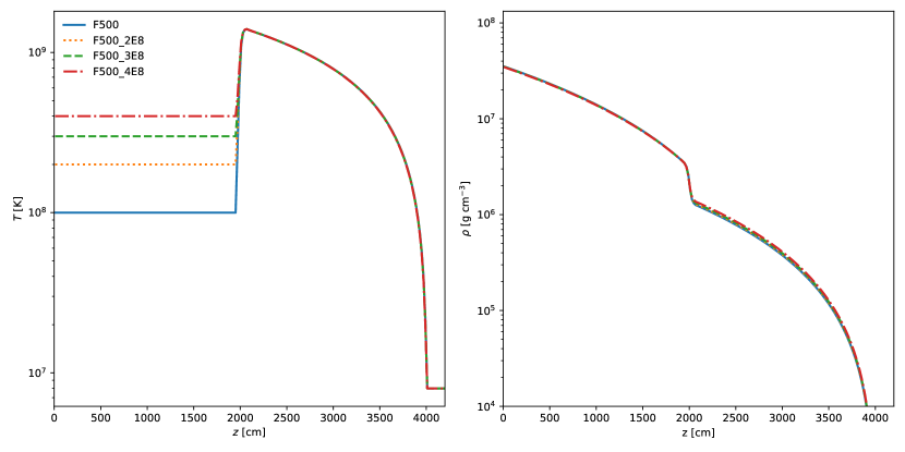
Figure 1: Initial temperature structure (left panel) and density structure (right panel) as a function of height in the “hot” state.

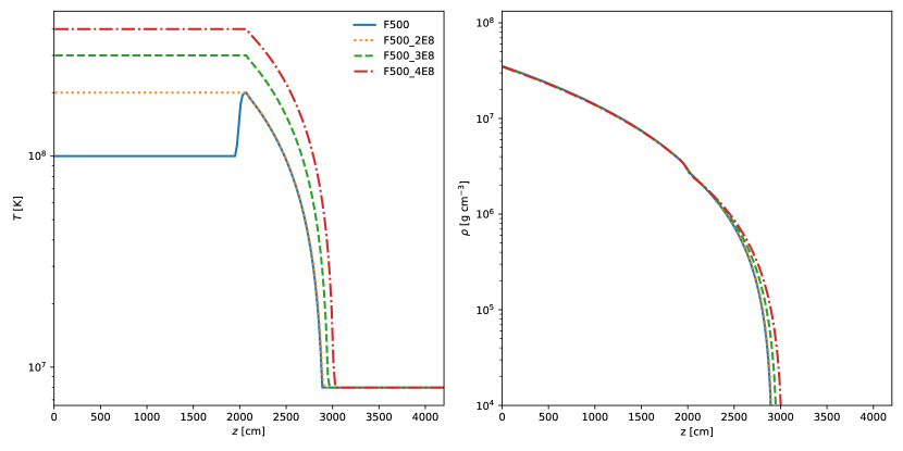
Figure 2: Initial temperature structure (left panel) and density structure (right panel) as a function of height in the “cool” state.

For the current simulations, we explore a variety of initial rotation rate and temperature conditions for the flame. The main parameters describing the models and the names by which we shall refer to them in this paper are provided in Table 1. Figure 1 shows the temperature and density structure for our hot models and Figure 2 shows the temperature and density structure for the cool models.

Table 1: Rotation rate and temperature properties of the simulations. In the left-hand column we list the names we shall use to refer to each simulation throughout this paper.

run	Rotation Rate (Hz)	$\delta T$ (K)	$T_{\mathrm{hi}}$ (K)	$T_{\mathrm{star}}$ (K)	$T_{\mathrm{lo}}$ (K)
F1000	$1000$	$1.2\times 10^{9}$	$2\times 10^{8}$	$10^{8}$	$8\times 10^{6}$
F500	$500$	$1.2\times 10^{9}$	$2\times 10^{8}$	$10^{8}$	$8\times 10^{6}$
F500_2E8	$500$	$1.2\times 10^{9}$	$2\times 10^{8}$	$2\times 10^{8}$	$8\times 10^{6}$
F500_3E8	$500$	$1.1\times 10^{9}$	$3\times 10^{8}$	$3\times 10^{8}$	$8\times 10^{6}$
F500_4E8	$500$	$10^{9}$	$4\times 10^{8}$	$4\times 10^{8}$	$8\times 10^{6}$
F250	$250$	$1.2\times 10^{9}$	$2\times 10^{8}$	$10^{8}$	$8\times 10^{6}$

3 Simulations and Results

We present six simulations in total, summarized in Table 1. These simulations encompass three different rotation rates: $250~{}\mathrm{Hz}$, $500~{}\mathrm{Hz}$, and $1000~{}\mathrm{Hz}$, and for the $500~{}\mathrm{Hz}$ run, four different temperature profiles. In the following subsections, we look at how the flame properties depend on the model parameters. All simulations are run in a domain of $1.8432\times 10^{5}~{}\mathrm{cm}\times 3.072\times 10^{4}~{}\mathrm{cm}$ with a coarse grid of $1152\times 192$ zones and two levels of refinement (the first level refining the resolution by factor of four, and the second by a factor of two again). This gives a fine-grid resolution of $20~{}\mathrm{cm}$. In these simulations, refinement is carried out in all zones within the atmosphere with density $\rho>2.5\times 10^{4}~{}\mathrm{g~{}cm^{-3}}$. We use an axisymmetric coordinate system, with the horizontal $r$-direction pointing along the surface of the star and the vertical $z$-direction pointing perpendicular to the surface.

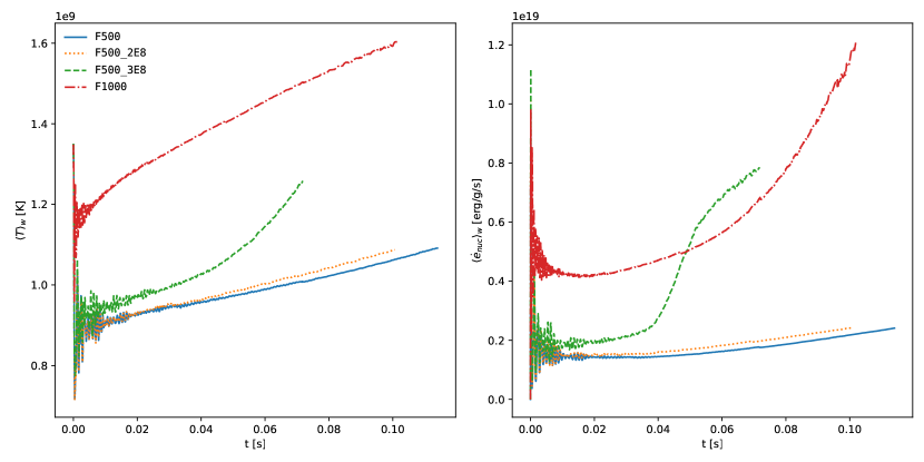
Figure 3: Estimates of temperature (left panel) and nuclear energy generation rate (right panel) in the burning region as functions of time. The quantities on the vertical axes are the mass-weighted averages defined in Equation 1.

For some of our analysis, we would like to have a means of estimating the temperature ($T$) and nuclear energy generation rate ($\dot{e}_{\rm nuc}$) in the burning region of each simulation. For this purpose, we define the mass-weighted average $\langle Q\rangle_{w}$ of some quantity $Q$ to be

$$\langle Q\rangle_{w}\equiv\frac{\sum_{c_{i}}m(c_{i})Q(c_{i})}{\sum_{c_{i}}m(c_{i})};~{}c_{i}\in C_{99}(Q).$$ (1)

Here, $C_{99}(Q)$ is the set of grid cells with $Q$ values in the top percentile, $Q(c_{i})$ is the value of $Q$ in cell $c_{i}$, and $m(c_{i})$ is the total mass in cell $c_{i}$. Using $\langle Q\rangle_{w}$ instead of simply taking the maximum of the quantity across the entire simulation domain allows us to track changes over the domain as a whole rather than at a single localized point. This will therefore be a better reflection of the overall behavior of the flame rather than of a single localized fluctuation. Figure 3 shows $\langle T\rangle_{w}$ and $\langle\dot{e}_{\rm nuc}\rangle_{w}$ as functions of time for the subset of our runs that achieve a propagating flame. This figure is referenced throughout the subsequent sections.

3.1 Effect of Rotation Rate on Flame Structure

We run three models (F250, F500, and F1000) with the same initial model in terms of temperature but differing rotation rates. We saw in Eiden et al. (2020) that increasing the neutron star rotation rate reduces the horizontal lengthscale of the flame. An estimate of this lengthscale is given by the Rossby radius of deformation, $L_{R}$. The Rossby radius may be thought of as the scale over which the balance between the Coriolis force and horizontal pressure gradient becomes important, and is approximately given by

$$L_{R}\approx\frac{\sqrt{gH_{0}}}{\Omega},$$ (2)

where $g$ is the gravitational acceleration, $H_{0}$ is the atmospheric scale height, and $\Omega$ is the neutron star rotation rate. In Figure 4 and Figure 5, we use $\dot{e}_{\mathrm{nuc}}$ measured at $50~{}\mathrm{ms}$ and $100~{}\mathrm{ms}$ to discern the horizontal extent of the flame at different rotation rates. Taking the edge at greatest radius of the bright teal/green region where the most significant energy generation is occurring as the leading edge of the flame in each plot, we see that the horizontal extent of the $1000~{}\mathrm{Hz}$ flame ($\tt{F1000}$) appears to be reduced compared to the lower rotation $500~{}\mathrm{Hz}$ run ($\tt{F500}$). From Equation 2, we can see that increasing the rotation rate from $500~{}\mathrm{Hz}$ to $1000~{}\mathrm{Hz}$ should decrease $L_{R}$ by a factor of two, and that the greater confinement from the Coriolis force should reduce the horizontal extent of the flame by a similar factor. However, the Rossby radius is only an approximate measure of this horizontal lengthscale, and in our simulations we see that this scaling does not work so well for all rotation rates. The simulations seem to follow the theoretical scaling described in Equation 2 more closely at higher rotation rates ($1000~{}\mathrm{Hz}$ and higher), based on the results of Eiden et al. (2020).

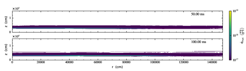
Figure 4: Time series of the $500~{}\mathrm{Hz}$ run F500 showing the nuclear energy generation rate, $\dot{e}_{\mathrm{nuc}}$.

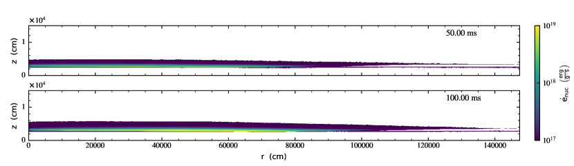
Figure 5: Time series of the $1000~{}\mathrm{Hz}$ run F1000 showing the nuclear energy generation rate, $\dot{e}_{\mathrm{nuc}}$.

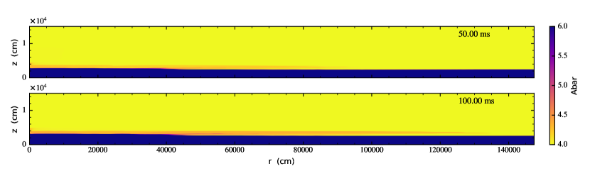
Figure 6: Time series of the $500~{}\mathrm{Hz}$ run F500 showing the mean molecular weight, $\bar{A}$.

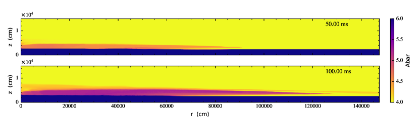
Figure 7: Time series of the $1000~{}\mathrm{Hz}$ run F1000 showing the mean molecular weight, $\bar{A}$.

The F500 and F1000 runs both qualitatively resemble the flame structure in Eiden et al. (2020) — a laterally propagating flame that is lifted off of the bottom of the fuel layer — but they differ in their burning structures. Figures 6 and 7 show time series of the mean molecular weight, $\bar{A}$, for the F500 and F1000 runs. Compared to those in Eiden et al. (2020), ashes behind the flame do not reach as high atomic weights. This is not surprising, since those previous runs artificially boosted the reaction rates. Comparing these two new runs, the burning is much more evolved for the higher rotation rate, and the ash is actually able to move ahead of the flame front (visible in the Figure 7 $100~{}\mathrm{ms}$ snapshot). We believe that this is because the increased rotation better confines the initial perturbation and subsequent expansion from the burning, increasing the temperature and density in the flame front such that the reaction rate increases, which allows the reactions to progress further. The $\dot{e}_{\mathrm{nuc}}$ plots in Figure 5 also support this interpretation, with the region of the flame front nearest to the crust in the F1000 run reaching higher $\dot{e}_{\mathrm{nuc}}$ values than for the F500 run in Figure 4. In contrast to F500 and F1000, the lowest rotation run — F250 — failed to ignite. The lack of ignition for F250 also aligns with the reasoning given above, with the lower rotation in this case potentially leading to insufficient confinement such that the temperature and density required for ignition is not achieved. In this scenario, another source of confinement (e.g. magnetic fields, see Cavecchi et al. (2016)) would need to take over at lower rotation rates to allow a burst to occur, at least for the initial model used here. Given that the size of our domain is $\sim 1~{}L_{R}$ for F250 (using Equation 2), it is also possible that we simply cannot confine the flame sufficiently with our current domain width. We see in Figure 11 (discussed further in Section 3.2) that the F500 flame took longer to achieve steady propagation than the F1000 flame. It may therefore also be that we did not run our simulation for long enough to see the F250 flame achieve the conditions required for ignition and steady propagation.

Burning in the F500 and F1000 runs is concentrated in a dense region with circular motion. In Figure 8, which compares the horizontal $r$-velocity $u$, density $\rho$ and the nuclear energy generation rate $\dot{e}_{\rm nuc}$ for the F250, F500, and F1000 runs, most of the burning for each of the simulations occurs in a high density region $\rho>3\times 10^{5}~{}{\rm g\,cm^{-3}}$. The fluid in this dense, high energy generation region undergoes vortical motion, shown in the Figure 9 phase plots comparing $u$, the vertical $z$-velocity $v$ and $\dot{e}_{\rm nuc}$. This most likely corresponds to the leading edge of the flame where fresh fuel is being entrained. This feature is not developed in the $250~{}\mathrm{Hz}$ flame in Figure 9 (left panel); it could potentially develop at later times (past the point at which we terminated our simulation), or the burning could just fizzle out and the flame fail to ignite entirely.

The mean molecular weight $\bar{A}$ within each of our simulations seems to grow along defined tracks confined to certain temperatures $T$, as shown in the Figure 10 phase plots. We believe that the tracks in the plot correspond to different burning trajectories in phase space resulting from different thermodynamic conditions. Comparing Figure 10 to Eiden et al. (2020), these tracks are much more neat and clearly defined. The “messiness” of the tracks may be dependent on how mixed the flame interior is. Since these new simulations are un-boosted, they may be inherently less mixed than those in Eiden et al. (2020). F1000 aligns with this interpretation: its $\bar{A}$ tracks are somewhat disrupted compared to the slower rotation runs, possibly due to the more vigorous mixing of the vortex at the flame front. Comparing the different runs, we also see that as the rotation rate increases, so does the peak temperature. This makes sense if higher rotation leads to a more concentrated, intense vortex near the flame front. It also agrees with our earlier interpretation of the enhanced burning seen in Figure 7 for F1000.

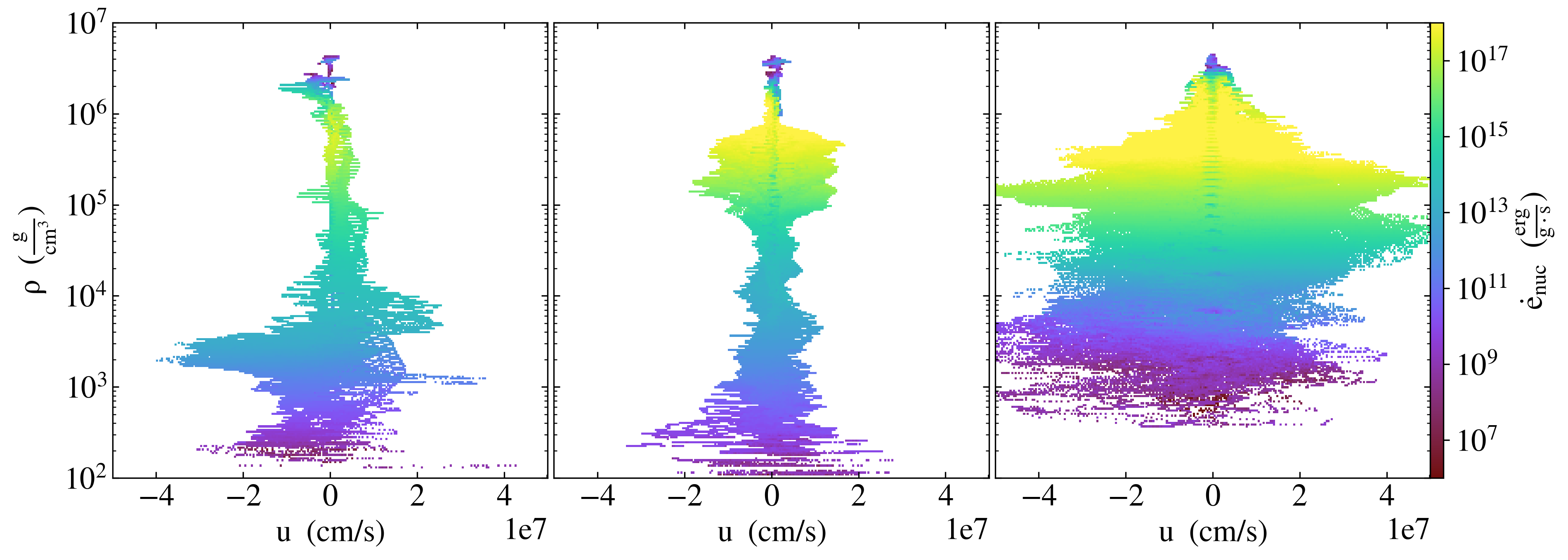
Figure 8: Phase plot of the horizontal $r$-velocity $u$, density $\rho$ and the nuclear energy generation rate $\dot{e}_{\rm nuc}$ for the 250, 500 and $1000~{}\mathrm{Hz}$ runs (F250, F500 and F1000) at $t=100~{}\mathrm{ms}$. The slightly lower $\dot{e}_{\rm nuc}$ values along the $u=0$ axis are most likely a numerical artifact related to the density gradient setup and finite resolution of these simulations.

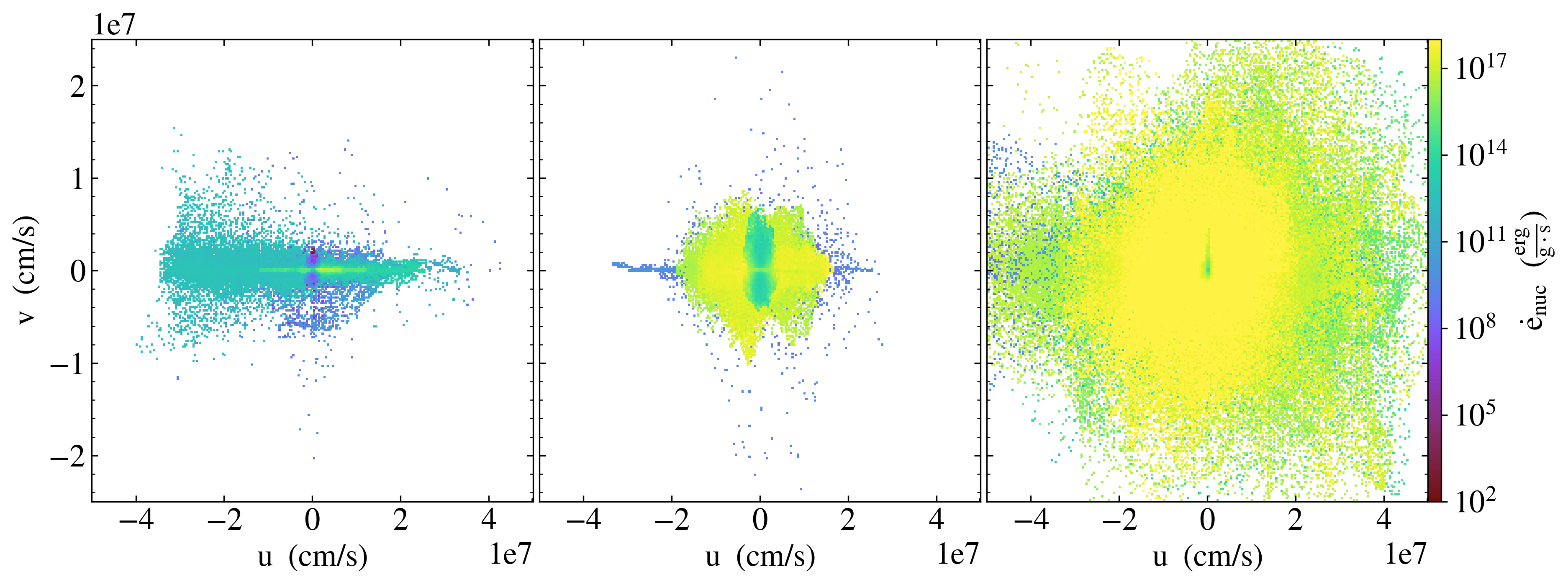
Figure 9: Phase plot of the horizontal $r$-velocity $u$, vertical $z$-velocity $v$ and the nuclear energy generation rate $\dot{e}_{\rm nuc}$ for the 250, 500 and $1000~{}\mathrm{Hz}$ runs (F250, F500 and F1000) at $t=100~{}\mathrm{ms}$.

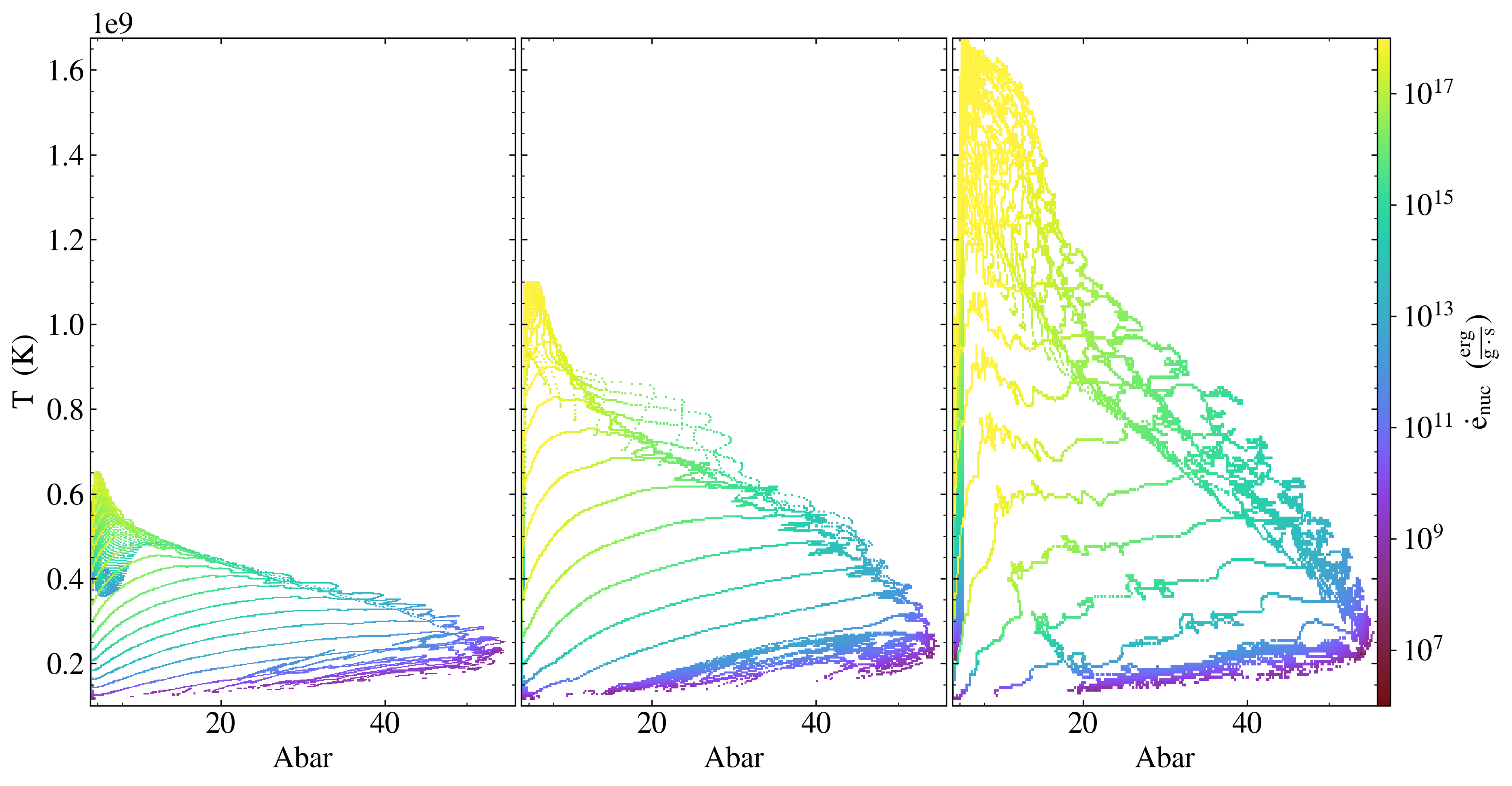
Figure 10: Phase plot of the mean molecular weight $\bar{A}$, temperature $T$ and the nuclear energy generation rate $\dot{e}_{\rm nuc}$ for the 250, 500 and $1000~{}\mathrm{Hz}$ runs (F250, F500 and F1000) at $t=100~{}\mathrm{ms}$.

3.2 Effect of Rotation Rate on Flame Propagation

For the purpose of measuring the flame propagation speed and acceleration, we track the position of each of our flames as a function of time. We define the position in terms of a specific value of the energy generation rate, $\dot{e}_{\rm nuc}$, as we did in Eiden et al. (2020). To recapitulate: we first reduce the 2D $\dot{e}_{\rm nuc}$ data for each simulation run to a set of 1D radial profiles by averaging over the vertical coordinate. After averaging, we take our reference $\dot{e}_{\rm nuc}$ value to be some fraction of the global $\dot{e}_{\rm nuc}$ maximum across all of these profiles. Since the flames in our simulations propagate in the positive horizontal direction, we then search the region of each profile at greater radius than the local $\dot{e}_{\rm nuc}$ maximum for the point where the $\dot{e}_{\rm nuc}$ first drops below this reference value. This point gives us the location of our flame front.

In Eiden et al. (2020), we used $0.1\%$ of the global $\dot{e}_{\rm nuc}$ maximum for our reference value. For the high temperature unboosted flames, however, we found that the $\dot{e}_{\rm nuc}$ profiles failed to reach that small a value across the domain at most times, which prevented us from obtaining reliable position measurements. We therefore use $1\%$ of the global $\dot{e}_{\rm nuc}$ maximum in this paper rather than $0.1\%$. This is still sufficiently small that our measurements are not overly sensitive to turbulence and other local fluid motions (the issue with simply tracking the local maximum), but allows us to avoid the pitfall encountered by the $0.1\%$ metric.

Table 2: Flame speed and acceleration values measured for each simulation. $v_{0}$ is the flame velocity in the $+r$ direction at $t=0~{}\mathrm{ms}$ and $a$ is the acceleration of the flame. The initial flame velocities and accelerations are derived from a quadratic least-squares fit to each of the datasets for times $t\gtrsim 20~{}\mathrm{ms}$. Using these fit parameters we calculate the velocity at $t=50~{}\mathrm{ms}$, $v_{50}$, at which point the flames have reached steady propagation.

run	$v_{0}$ (km s-1)	$a$ (km s-2)	$v_{50}$ (km s-1)
F1000	$3.414\pm 0.008$	$-1.03\pm 0.13$	$3.36\pm 0.01$
F500	$3.077\pm 0.013$	$5.41\pm 0.19$	$3.35\pm 0.02$
F500_2E8	$3.760\pm 0.015$	$1.74\pm 0.25$	$3.85\pm 0.02$
F500_3E8	$-5.293\pm 0.100$	$357.41\pm 2.15$	$12.58\pm 0.15$

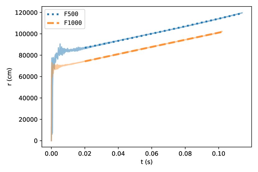
Figure 11: Flame front position vs. time for the standard ($10^{8}~{}\mathrm{K}$) $500~{}\mathrm{Hz}$ and $1000~{}\mathrm{Hz}$ runs (F500 and F1000). The dashed lines show quadratic least-squares fits to the data for $t\gtrsim 20~{}\mathrm{ms}$.

Figure 11 gives the radial position of the flame front as a function of time for the $\tt{F500}$ and $\tt{F1000}$ runs (blue and orange, respectively) to show the dependence on rotation rate. In Eiden et al. (2020), we applied a linear least-squares fit to the flame front position as a function of time to estimate the propagation velocity. As some of the flames in this set of simulation runs exhibit significant acceleration, for this study we instead fit the data with a quadratic curve of the form

$$r(t)=\frac{1}{2}at^{2}+v_{0}t+r_{0},$$ (3)

where the parameter $a$ is the acceleration of the flame, $v_{0}$ is the velocity at $t=0~{}\mathrm{ms}$, and $r_{0}$ is the flame front position at $t=0~{}\mathrm{ms}$. We do not include the data points with $t\lesssim 20~{}\mathrm{ms}$ when performing the fit, since these correspond to the initial transient period before the flame has begun to propagate steadily. The values of $a$ and $v_{0}$ for the full suite of simulation runs are provided in Table 2. Note that $v_{0}$ is only a parameter that may be used to calculate the flame speed at an arbitrary time. It is not an estimate of the true initial velocity of the flame, since the flame has not achieved ignition yet at $t=0~{}\mathrm{ms}$. We use the fit parameters to calculate the flame speeds at $t=50~{}\mathrm{ms}$ (when the flame has reached steady propagation), given in the fourth column of Table 2.

, and as seen in Figure 11, there is no clear inverse scaling of the flame speed with rotation rate in the new set of runs. We observed earlier, however, that nuclear reactions progress more quickly at higher rotation rate. This results in a higher $\dot{e}_{\rm nuc}$ — up to three to four times higher near the burning front after the flame ignites (see Figure 3) — which may counteract the reduction in flame speed from the increased Coriolis confinement. Comparing accelerations, we also observe that $\tt{F500}$ accelerates faster than $\tt{F1000}$, which appears to experience a small deceleration at early times. This disparity may be a direct result of the difference in Coriolis force.

3.3 Effect of Temperature on Flame Structure

To explore the effect of different initial temperature configurations, we run four simulations fixed at a rotation rate of $500~{}\mathrm{Hz}$ with temperatures as shown in Table 1. For all the $500~{}\mathrm{Hz}$ simulations (with the exception of the coolest run, $\tt{F500}$), we set $T_{\mathrm{star}}$ = $T_{\mathrm{hi}}$, scaling $\delta T$ accordingly to maintain a consistent value of $T_{\mathrm{hi}}+\delta T$. If we let $T_{\mathrm{star}}<T_{\mathrm{hi}}$, the cooler neutron star surface might act as a heat sink and siphon away energy that would otherwise go into heating the burning layer. By choosing $T_{\mathrm{star}}$ = $T_{\mathrm{hi}}$, we can effectively explore simulations with greater surface heating. There are several physically distinct mechanisms that could produce an increased temperature at the crust: crustal heating, some other form of shallow heating or accretion-induced heating. In these simulations, we do not model the mechanism producing the heating effect, just the effect itself, so we do not distinguish between which of these mechanisms cause the heating.

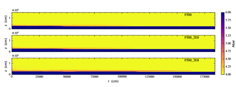
Figure 12: Comparison of $\bar{A}$ for 3 different $500~{}\mathrm{Hz}$ models with neutron star temperatures $T_{\rm star}$ of $10^{8}~{}\mathrm{K}$, $2\times 10^{8}~{}\mathrm{K}$ and $3\times 10^{8}~{}\mathrm{K}$ ($\tt{F500}$, $\tt{F500\_2e8}$, and $\tt{F500\_3e8}$, respectively), and resulting envelope structures. Each flame is shown at $70~{}\mathrm{ms}$.

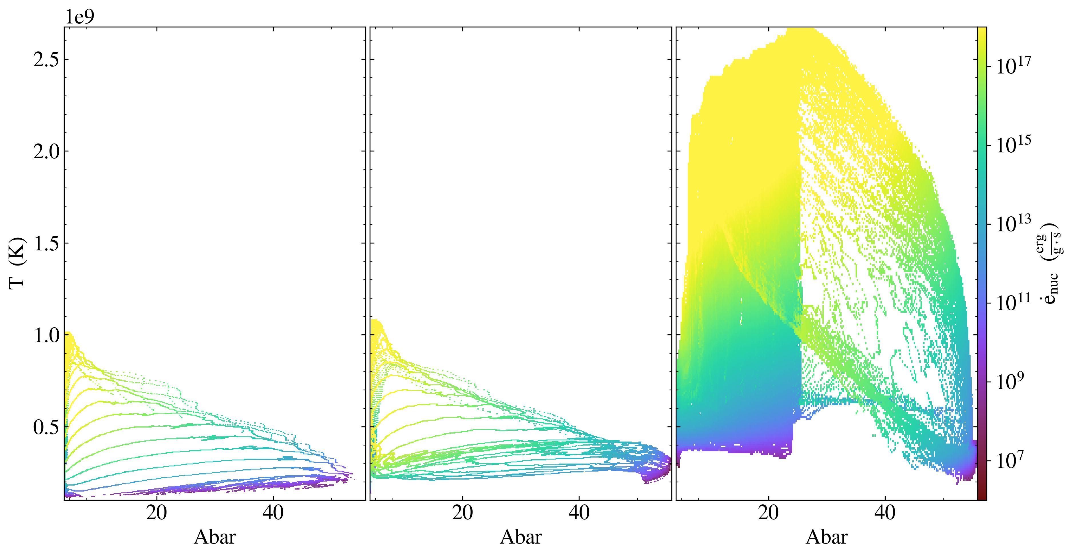
Figure 18: Phase plot of the mean molecular weight $\bar{A}$, temperature $T$ and the nuclear energy generation rate $\dot{e}_{\rm nuc}$ for the $500~{}\mathrm{Hz}$ runs with $T_{\rm star}$ of $10^{8}~{}\mathrm{K}$, $3\times 10^{8}~{}\mathrm{K}$ and $4\times 10^{8}~{}\mathrm{K}$ ($\tt{F500}$, $\tt{F500\_3e8}$, and $\tt{F500\_4e8}$) at $t=40~{}\mathrm{ms}$. The run with $T_{\rm star}=2\times 10^{8}~{}\mathrm{K}$ ($\tt{F500\_2E8}$) closely resembles the cooler $\tt{F500}$ run, and is not shown here.

Figure 12 shows $\bar{A}$ for three $500~{}\mathrm{Hz}$ simulations with different initial temperature structures ($T_{\mathrm{star}}\leq 3\times 10^{8}~{}\mathrm{K}$) at $t=70~{}\mathrm{ms}$. We do not plot $\tt{F500\_4E8}$ here because it fails to form a clear burning front. $\tt{F500\_3E8}$ (Figure 12, bottom panel) — the hottest run to form a clear burning front — has a faster propagating flame (this will be discussed further in Section 3.4). It also reaches slightly higher $\bar{A}$ values than the two cooler runs. The Figure 18 $\bar{A}$-$T$ phase plots of $\tt{F500}$ (left) and $\tt{F500\_3E8}$ (middle) also reflect these $\bar{A}$ features, with $\tt{F500\_3E8}$ reaching slightly higher $\bar{A}$ values. $\tt{F500\_3E8}$ also reaches higher $\dot{e}_{\rm nuc}$ values at the low end of the temperature range ($<0.5\times 10^{9}~{}\mathrm{K}$). There appear to be more causally connected regions across a range of $\bar{A}$ at low temperatures for $\tt{F500\_3E8}$ than for $\tt{F500}$, suggesting that the higher $\dot{e}_{\rm nuc}$ for $\tt{F500\_3E8}$ generates burning in certain burning trajectories that are not present in the cooler $\tt{F500}$ run. Note that, although $\tt{F500\_3E8}$ is the hottest run with a modified initial temperature configuration to form a distinct flame front, the highest rotation $\tt{F1000}$ flame actually reaches higher temperatures (see Figure 3, left panel) as well as higher $\bar{A}$ (see Figure 7).

In contrast to the models with $T_{\mathrm{star}}\leq 3\times 10^{8}~{}\mathrm{K}$, $\tt{F500\_4E8}$ is so hot that the organized flame structure is lost. This model burns so strongly that it is only run out to $40~{}\mathrm{ms}$. After an initial period when the burning moves across the domain, residual burning continues and eventually ignites the entire fuel layer at late times, as shown in Figures 13 and 14 for three snapshots taken in the last ten seconds of the simulation. In Figure 13, $\dot{e}_{\rm nuc}$ reaches values of $10^{18}-10^{20}~{}\mathrm{erg}\,\mathrm{g}^{-1}\mathrm{s}^{-1}$ across the domain and at heights up to $\sim 0.5\times 10^{4}~{}\mathrm{cm}$. There is still significant burning occurring even higher, with $\dot{e}_{\rm nuc}$ reaching $\sim 10^{15}~{}\mathrm{erg}\,\mathrm{g}^{-1}\mathrm{s}^{-1}$ at heights up to $\sim 0.8\times 10^{4}~{}\mathrm{cm}$. For comparison, the next hottest run ($\tt{F500\_3E8}$) only reaches maximum $\dot{e}_{\rm nuc}$ values on the order of $10^{18}~{}\mathrm{erg}\,\mathrm{g}^{-1}\mathrm{s}^{-1}$ (see Figure 3, right panel), even at the latest timesteps ($\sim 70~{}\mathrm{ms}$, when the flame is most developed). Significant $\dot{e}_{\rm nuc}$ values for all runs other than $\tt{F500\_4E8}$ are confined to the flame front, rather than spanning the entire domain.

Figure 14 shows $\bar{A}$ for $\tt{F500\_4E8}$. Again, burning extends across the domain and high into the atmosphere and fuel layer, lacking the characteristic flame structure shown in $\bar{A}$ plots for the lower temperature $500~{}\mathrm{Hz}$ runs (see Figure 12). A distinct mass of material appears to have broken out of the atmosphere near the axis of symmetry. The atmosphere edge is located at $\sim 1.2\times 10^{4}~{}\mathrm{cm}$. A similar effect is also visible (to a lesser extent) in the $\tt{F500\_3E8}$ plot in Figure 12, with a faint haze of material rising above the flame near the axis of symmetry. However, this is likely to be a numerical artefact rather than a true physical effect, and a result of the boundary conditions imposed at the axis of symmetry for these simulations. $\tt{F500\_4E8}$ clearly reaches much higher $\bar{A}$ values across the domain (especially at the latest snapshot, $t=40~{}\mathrm{ms}$) compared to all the other runs described in this paper (see Figures 6, 7 and 12).

Though $\tt{F500\_4E8}$ does not form a distinct burning front, it does achieve greatly enhanced burning, as shown in the Figure 18 $\bar{A}$-$T$ phase plot (right panel). Not only is $\tt{F500\_4E8}$ significantly hotter overall compared to all other runs, but there is a large causally connected region across a wide range of $\bar{A}$. This indicates that the hotter temperature has facilitated significant burning in burning trajectories that were not favored at the lower temperatures. The burning trajectories are also very disrupted for $\tt{F500\_4E8}$ compared to the cooler runs, suggesting that the hotter temperature leads to more vigorous mixing. Indeed, this appears to be the case looking at Figure 14 and the right panel of Figure 17 (discussed further in section 3.4). The disrupted burning trajectories resemble those found in Figure 10 for the highest rotation $\tt{F1000}$ run, though they are even more dramatically disrupted for $\tt{F500\_4E8}$. $\tt{F500\_4E8}$ is also noticeably hotter than $\tt{F1000}$, even though it is run for significantly less time ($t=40~{}\mathrm{ms}$ vs $t=100~{}\mathrm{ms}$). Although the $\tt{F500\_4E8}$ run is clearly a special case in that it develops steady burning across the domain rather than a propagating flame, enhanced burning in this hottest run aligns with results from the other simulations with differing initial temperature structures. As $T_{\mathrm{star}}$ is increased, the overall behavior and propagation of the flame is significantly altered, implying that burning is very temperature-sensitive. We explore flame propagation further in Section 3.4.

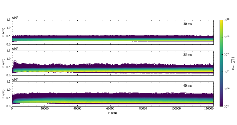
Figure 13: Time series of the $500~{}\mathrm{Hz}$ run $\tt{F500\_4E8}$, with $T_{\mathrm{star}}=4\times 10^{8}~{}\mathrm{K}$, showing $\dot{e}_{\rm nuc}$. This model burns so strongly that it is only run out to $40~{}\mathrm{ms}$; the snapshots shown here are at $T=30~{}\mathrm{ms}$, $35~{}\mathrm{ms}$, and $40~{}\mathrm{ms}$.

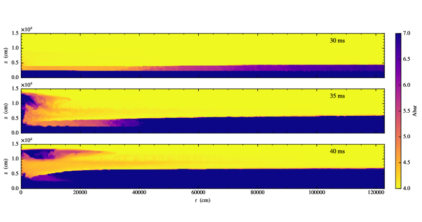
Figure 14: Time series of the $500~{}\mathrm{Hz}$ run $\tt{F500\_4E8}$, with $T_{\mathrm{star}}=4\times 10^{8}~{}\mathrm{K}$, showing $\bar{A}$.

3.4 Effect of Temperature on Flame Propagation

The method for measuring flame propagation described in Section 3.2 is applied in Figure 15 to the three $500~{}\mathrm{Hz}$ runs with $T_{\mathrm{star}}\leq 3\times 10^{8}~{}\mathrm{K}$. Due to the lack of a clear burning front in $\tt{F500\_4E8}$, we do not analyze its propagation velocity and acceleration. As the initial $T_{\mathrm{star}}$ is increased beyond $\sim 2\times 10^{8}~{}\mathrm{K}$, the flame becomes greatly accelerated. The initial flame velocities and accelerations derived from a quadratic least-squares fit to each of the datasets, as well as the flame velocities at $t=50~{}\mathrm{ms}$ calculated using the fit parameters, are provided in Table 2. Comparing the flame propagation at different initial temperatures, the most robust feature is the acceleration of the $\tt{F500\_3E8}$ run at $t\sim 40~{}\mathrm{ms}$. The reason for the acceleration of the flame is not entirely clear. Whereas for the cooler runs, a state of steady flame propagation is achieved, for the $\tt{F500\_3E8}$ run the flame speed continues to increase, suggesting that some instability driving the flame’s propagation persists to later times. It could be that energy released from burning begins to dominate the flame’s propagation as it evolves, increasing the flame speed over time. Another possibility is that the increased temperatures lead to enhanced turbulent mixing effects that pull in more fresh fuel for the flame to burn. Yet another possibility is that the higher initial $T_{\mathrm{star}}$ leads to a greater average temperature in the fuel layer over time, making it easier for the flame to burn the fuel and propagate.

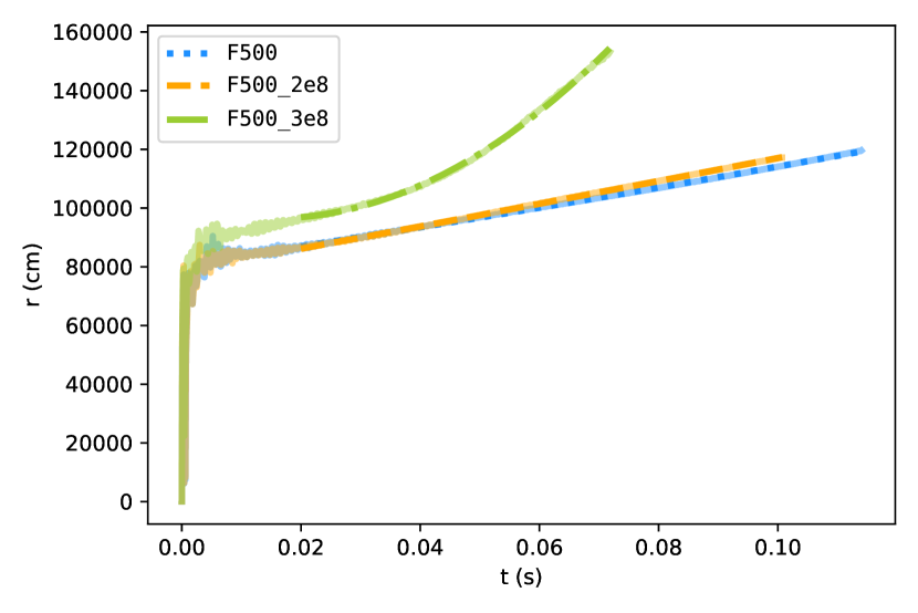
Figure 15: Flame front position vs. time for the three $500~{}\mathrm{Hz}$ runs with $T_{\rm star}$ of $10^{8}~{}\mathrm{K}$, $2\times 10^{8}~{}\mathrm{K}$ and $3\times 10^{8}~{}\mathrm{K}$ ($\tt{F500}$, $\tt{F500\_2e8}$, and $\tt{F500\_3e8}$, respectively). The dashed lines show quadratic least-squares fits to the data for $t\gtrsim 20~{}\mathrm{ms}$. Note that due to its rapid acceleration, $\tt{F500\_3E8}$ (green) is only run out to $\sim 70~{}\mathrm{ms}$ to avoid surpassing the domain boundary.

In both the $u$-$\rho$ phase plot in Figure 16 and the $u$-$v$ phase plot in Figure 17, the horizontal $u$-velocity for the $\tt{F500\_4e8}$ (right panel) burning region is slightly larger than that of the cooler runs. Additionally, the cooler runs’ $u$-velocities are two to three orders of magnitude greater than the flame speeds listed in Table 2. These phase plot velocities therefore most likely correspond to vortical motion in the turbulent burning vortices rather than the propagation of a flame itself. The vertical $z$-velocity $v$ in Figure 17 further suggests that $\tt{F500\_4e8}$ undergoes increased vortical motion, as we see that the velocity magnitude in the burning region is significantly larger than in the lower temperature runs. Also of interest in these plots is that the coolest run shows high velocity material comprising both high and low $\dot{e}_{\rm nuc}$ with horizontal velocity asymmetry, both of which suggest the burning vortex in the coolest case is less well defined than at higher temperatures. The coolest run thus does not seem to have developed the characteristic vortex structure at the burning front (i.e. where $\dot{e}_{\rm nuc}$ is greatest) that can be clearly seen for the hotter runs at this time ($40~{}\mathrm{ms}$). As can be seen in Figure 9 (which was plotted at $100~{}\mathrm{ms}$), this does develop more at later times. Similar to what we saw when comparing the runs with different rotation rates, it would therefore appear that it takes longer for the flame to develop when $T_{\rm star}$ is cooler.

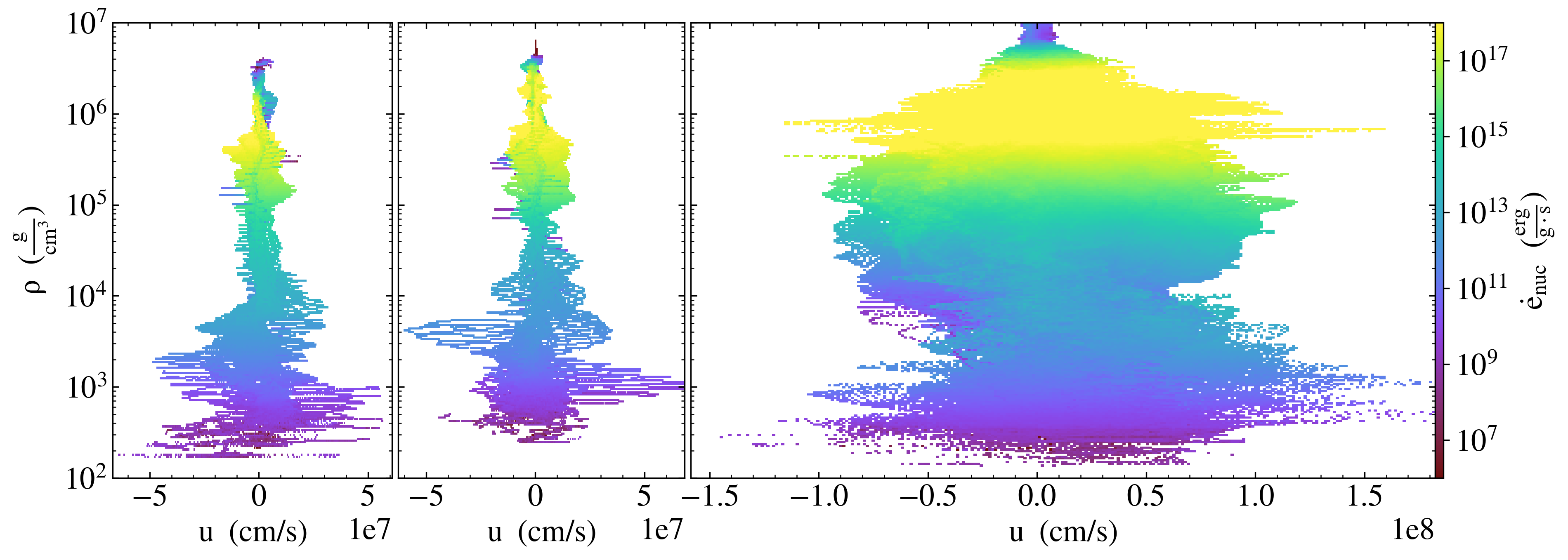
Figure 16: Phase plot of the horizontal $r$-velocity $u$, density $\rho$ and the nuclear energy generation rate $\dot{e}_{\rm nuc}$ for the $500~{}\mathrm{Hz}$ runs with $T_{\rm star}$ of $10^{8}~{}\mathrm{K}$, $3\times 10^{8}~{}\mathrm{K}$ and $4\times 10^{8}~{}\mathrm{K}$ ($\tt{F500}$, $\tt{F500\_3e8}$, and $\tt{F500\_4e8}$) at $t=40~{}\mathrm{ms}$ (the latest time that $\tt{F500\_4E8}$ is run out to). The run with $T_{\rm star}=2\times 10^{8}~{}\mathrm{K}$ ($\tt{F500\_2E8}$) closely resembles the cooler $\tt{F500}$ run, and is not shown here.

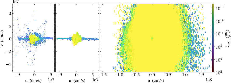
Figure 17: Phase plot of the horizontal $r$-velocity $u$, vertical $z$-velocity $v$ and the nuclear energy generation rate $\dot{e}_{\rm nuc}$ for the $500~{}\mathrm{Hz}$ runs with $T_{\rm star}$ of $10^{8}~{}\mathrm{K}$, $3\times 10^{8}~{}\mathrm{K}$ and $4\times 10^{8}~{}\mathrm{K}$ ($\tt{F500}$, $\tt{F500\_3e8}$, and $\tt{F500\_4e8}$) at $t=40~{}\mathrm{ms}$. The run with $T_{\rm star}=2\times 10^{8}~{}\mathrm{K}$ ($\tt{F500\_2E8}$) closely resembles the cooler $\tt{F500}$ run, and is not shown here.

4 Discussion and Conclusions

We ran a number of simulations of laterally propagating flames in XRBs in order to explore the effects of rotation and thermal structure. We found that increasing the rotation rate increased the energy generation rate within the flame and enhanced nuclear burning. Apart from the lowest rotation run (which failed to ignite), flame propagation was not noticeably impacted by rotation rate; by the time the different flame fronts reached steady propagation, they shared comparable velocities. These results are likely due to the rotation-dependent strength of the Coriolis force and its confinement of the flame balancing the enhanced nuclear burning.

We explored several models with different crustal temperatures to determine what effects mechanisms such as higher accretion rates, crustal heating and shallow heating may have on flame propagation. We found that increasing the temperature of the crust significantly enhanced the flame propagation. This we believe to be because a cooler crust allows heat to more efficiently be transferred away from the flame itself, therefore reducing the flame’s temperature, slowing burning and consequently reducing its propagation speed. At higher crustal temperatures, we saw that the inability for heat to be efficiently transported away from the flame front increased the flame temperature, driving unstable, accelerating flame propagation. We saw that if the crust temperature was too high, then instead of a flame the entire atmosphere would burn steadily. This is reminiscent of what is seen for neutron stars with accretion rates exceeding the Eddington limit.

In future work, we would like to improve and expand our simulations in order to better understand the processes at play and to include more physics. This includes adding tracer particles to the simulations so we can monitor the fluid motion and perform more detailed nucleosynthesis; extending our simulations to 3D, which would hopefully alleviate some of the boundary effects we have observed in these simulations but will require significant computational resources; and exploring the resolution of our simulations more so that we can ensure that we have resolved all of the necessary physical processes. We would also like to model H/He flames, as these are the sites of rp-process nucleosynthesis (Schatz et al., 2001). Initially we will use the same reaction sequence explored in our previous convection calculations (Malone et al., 2014). Finally, we recently added an MHD solver to Castro (Barrios Sazo, 2020); this will allow us in the future to explore the effects of magnetic fields on flame propagation in XRBs.

References

- Almgren et al. (2020) Almgren, A., Sazo, M. B., Bell, J., et al. 2020, Journal of Open Source Software, 5, 2513, doi: 10.21105/joss.02513
- Almgren et al. (2010) Almgren, A. S., Beckner, V. E., Bell, J. B., et al. 2010, ApJ, 715, 1221, doi: 10.1088/0004-637X/715/2/1221
- Altamirano et al. (2010) Altamirano, D., Watts, A., Kalamkar, M., et al. 2010, ATel, 2932, 1
- Barrios Sazo (2020) Barrios Sazo, M. G. 2020, PhD thesis, State University of New York at Stony Brook
- Bernard-Champmartin et al. (2012) Bernard-Champmartin, A., Braeunig, J.-P., & Ghidaglia, J.-M. 2012, Computers and Fluids, 7, doi: 10.1016/j.compfluid.2012.09.014
- Bhattacharyya & Strohmayer (2007) Bhattacharyya, S., & Strohmayer, T. E. 2007, 666, L85, doi: 10.1086/521790
- Bildsten (1998) Bildsten, L. 1998, in ASIC, Vol. 515, 419
- Bilous & Watts (2019) Bilous, A. V., & Watts, A. L. 2019, 245, 19, doi: 10.3847/1538-4365/ab2fe1
- Brown et al. (1989) Brown, P. N., Byrne, G. D., & Hindmarsh, A. C. 1989, SIAM J. Sci. Stat. Comput., 10, 1038
- Cavecchi et al. (2016) Cavecchi, Y., Levin, Y., Watts, A. L., & Braithwaite, J. 2016, MNRAS, 459, 1259, doi: 10.1093/mnras/stw728
- Cavecchi et al. (2013) Cavecchi, Y., Watts, A. L., Braithwaite, J., & Levin, Y. 2013, MNRAS, 434, 3526, doi: 10.1093/mnras/stt1273
- Cavecchi et al. (2015) Cavecchi, Y., Watts, A. L., Levin, Y., & Braithwaite, J. 2015, MNRAS, 448, 445, doi: 10.1093/mnras/stu2764
- Chakraborty & Bhattacharyya (2014) Chakraborty, M., & Bhattacharyya, S. 2014, ApJ, 792, 4, doi: 10.1088/0004-637X/792/1/4
- Cumming et al. (2006) Cumming, A., Macbeth, J., Zand, J. J. M. i. T., & Page, D. 2006, The Astrophysical Journal, 646, 429, doi: 10.1086/504698
- Deibel et al. (2015) Deibel, A., Cumming, A., Brown, E. F., & Page, D. 2015, ApJ, 809, L31, doi: 10.1088/2041-8205/809/2/L31
- Eiden et al. (2020) Eiden, K., Zingale, M., Harpole, A., et al. 2020, ApJ, 894, 6, doi: 10.3847/1538-4357/ab80bc
- Fujimoto et al. (1981) Fujimoto, M. Y., Hanawa, T., & Miyaji, S. 1981, Astrophysical Journal, 247, 267, doi: 10.1086/159034
- Galloway et al. (2020) Galloway, D. K., in ’t Zand, J. J. M., Chenevez, J., et al. 2020, arXiv e-prints, arXiv:2003.00685. https://arxiv.org/abs/2003.00685
- Hunter (2007) Hunter, J. D. 2007, Computing in Science and Engg., 9, 90, doi: 10.1109/MCSE.2007.55
- Johnston et al. (2019) Johnston, Z., Heger, A., & Galloway, D. K. 2019, arXiv e-prints, arXiv:1909.07977. https://arxiv.org/abs/1909.07977
- Katz et al. (2020) Katz, M. P., Almgren, A., Sazo, M. B., et al. 2020, in Proceedings of the International Conference for High Performance Computing, Networking, Storage and Analysis, SC ’20 (IEEE Press)
- Keek & Heger (2017) Keek, L., & Heger, A. 2017, The Astrophysical Journal, 842, 113, doi: 10.3847/1538-4357/aa7748
- Keek et al. (2009) Keek, L., Langer, N., et al. 2009, Astronomy & Astrophysics, 502, 871
- Kluyver et al. (2016) Kluyver, T., Ragan-Kelley, B., Pérez, F., et al. 2016, in Positioning and Power in Academic Publishing: Players, Agents and Agendas, 87–90, doi: 10.3233/978-1-61499-649-1-87
- Malone et al. (2014) Malone, C. M., Zingale, M., Nonaka, A., Almgren, A. S., & Bell, J. B. 2014, ApJ, 788, 115, doi: 10.1088/0004-637X/788/2/115
- Nethercote & Seward (2007) Nethercote, N., & Seward, J. 2007, in Proceedings of the 28th ACM SIGPLAN Conference on Programming Language Design and Implementation, PLDI ’07 (New York, NY, USA: ACM), 89–100, doi: 10.1145/1250734.1250746
- Oliphant (2007) Oliphant, T. E. 2007, Computing in Science and Engg., 9, 10, doi: 10.1109/MCSE.2007.58
- Schatz et al. (2001) Schatz, H., Aprahamian, A., Barnard, V., et al. 2001, Physical Review Letters, 86, 3471, doi: 10.1103/PhysRevLett.86.3471
- Spitkovsky et al. (2002) Spitkovsky, A., Levin, Y., & Ushomirsky, G. 2002, ApJ, 566, 1018, doi: 10.1086/338040
- Timmes (2000) Timmes, F. X. 2000, ApJ, 528, 913, doi: 10.1086/308203
- Timmes & Woosley (1992) Timmes, F. X., & Woosley, S. E. 1992, ApJ, 396, 649, doi: 10.1086/171746
- Turk et al. (2011) Turk, M. J., Smith, B. D., Oishi, J. S., et al. 2011, ApJS, 192, 9, doi: 10.1088/0067-0049/192/1/9
- Turlione et al. (2015) Turlione, A., Aguilera, D. N., & Pons, J. A. 2015, Astronomy and Astrophysics, 577, doi: 10.1051/0004-6361/201322690
- van der Walt et al. (2011) van der Walt, S., Colbert, S. C., & Varoquaux, G. 2011, Computing in Science & Engineering, 13, 22, doi: 10.1109/MCSE.2011.37
- Zhang et al. (2019) Zhang, W., Almgren, A., Beckner, V., et al. 2019, Journal of Open Source Software, 4, 1370, doi: 10.21105/joss.01370