Error estimates for the Smagorinsky turbulence model: enhanced stability through scale separation and numerical stabilization

Abstract.

In the present work we show some results on the effect of the Smagorinsky model on the stability of the associated perturbation equation. We show that in the presence of a spectral gap, such that the flow can be decomposed in a large scale with moderate gradient and a small amplitude fine scale with arbitratry gradient, the Smagorinsky model admits stability estimates for perturbations, with exponential growth depending only on the large scale gradient. We then show in the context of stabilized finite element methods that the same result carries over to the approximation and that in this context, for suitably chosen finite element spaces the Smagorinsky model acts as a stabilizer yielding close to optimal error estimates in the $L^{2}$-norm for smooth flows in the pre-asymptotic high Reynolds number regime.

1. Introduction

The modelling and accurate approximation of turbulent flows at high Reynolds numbers remain an outstanding challenge. One of the earliest attempts at the design of a turbulence model is the one attributed to Smagorinsky [36, 37], where a nonlinear viscosity replaces the Reynolds stresses, thereby providing closure to the filtered Navier-Stokes’ equations. The model is believed to be inspired by early work on shock capturing methods for conservation laws due to Von Neumann and Richtmyer [39].

An appealing feature is that it has been shown that the Navier-Stokes’ equations regularized system admits a unique solution [31], with enhanced regularity [5, 6]. It has also been shown using scaling arguments that away from boundary layers the dissipation rate matches the Kolmogorov decay rate [32] for uniformly turbulent flows. On the other hand the Smagorinsky model is considered to be too dissipative, in particular in the laminar zone. The parameter of the model has to be tuned differently to obtained the best results depending the flow problem [22] and on the numerical method used [34], pointing to a subtle interplay between the flow and the numerical method for the performance of the Smagorinsky model in LES. Nevertheless thanks to its simplicity and its physical consistency, the Smagorinsky model remains an important tool for the modelling of turbulent high Reynolds flows.

The objective of the present work is to show some results on the effect of the Smagorinsky model on the stability of the fluid dynamics and on numerical approximation. We show that in the presence of a spectral gap, such that the flow can be decomposed in a large scale with moderate gradient and a small amplitude fine scale with arbitrary gradient, the Smagorinsky model admits stability estimates with exponential growth depending only on the large scale gradient. We then show in the context of stabilized finite element methods that the same result carries over to the approximation and that in this context, for suitably chosen finite element spaces the Smagorinsky model acts as a stabilizer yielding optimal error estimates for smooth flows in the high Reynolds number regime. This gives some evidence that the Smagorinsky model is efficient in situations where the flow has a clearly defined spectral gap. This is not in general the case for turbulent flows, but is believed to occur at high Reynolds number, near rough surfaces or the atmospheric boundary layer [21], or more generally in atmospheric and geophysical flows [20, 40, 35]. Interestingly, this is the context for which the Smagoringsky model was originally proposed [36].

The notion of Large Eddy Simulation (LES) is not very well defined. Depending on the context it is considered either as a modelling issue, or a numerical technique. In the first case the partial differential equation is perturbed by adding terms that model the so-called Reynolds stress term expressing the effect of unresolved scales, where the smallest length scale is a model parameter. The regularized model should be well-posed and can then be discretized. The challenge here is on the modelling side: how can one design a model that allows for a more stable representation of quantities of interests? Observe that to distinguish this method from the situation where the turbulence model is used for numerical stability, the model parameters should be fixed before discretization and not coupled to the mesh-size. In case such a coupling is introduced it would need to be justified, in particular in the asymptotic limit. A typical requirement is that the physically relevant solution, or a so-called “suitable” solution is obtained in the limit [24]. For so called numerical LES, or Implicit LES, on the other hand [9], the Navier-Stokes’ equations are considered, but a numerically stable discretization method is used ensuring that sufficient dissipation is added for the numerical scheme to remain stable, but not so much that smooth structures of the flow are destroyed. The underpinning idea is that any quantity of interest that has sufficient stability properties will then be computable [27, 10], if the numerical method resolves a sufficient range of scales so that the effect of unresolved scales is negligible. To be able to claim that an analysis of a LES method is successful it is necessary to address the question of stability, but there appears to be no stability estimates with moderate exponential growth, for any quantity of interest for the Navier-Stokes equations in the high Reynolds number regime. The best rigorous result of quantitative bound of perturbation growth in the inviscid regime appears to be [1], where a two-dimensional flow is analyzed and the stability constant grows with a double exponential in time.

Finite element analysis typically relies on the velocities having bounded gradients [30, 26], with a slight improvement possible in the two-dimensional case using parabolic regularization of the viscous scales [10]. Typically the stability constant is on the form $\exp(KT)$, with $K$ proportional to the maximum gradient of the velocity in the flow.

For the discussion below we will for simplicity consider the $p$-Laplacian model that acts on the whole gradient instead of the symmetric gradient as in the Smagorinsky case. This regularization was introduced in [33, Chap. 2, sec. 5], where also existence and uniqueness of solutions were studied. The below arguments can however easily be extended to the more common versions of the Smagorinsky model using the deformation tensor. The only essential difference is the need to apply Korn’s inequality in $L^{p}$, see for instance [16, Chapter 7] to get control of the gradient of the solution in $L^{p}$ through the control of its symmetric part.

Main results and outline

There appears to be very little known about the stability properties of the Smagorinsky model, or for that matter its qualities as a stabilizing term for numerical methods for high Reynolds flow in the laminar regime. In this paper we will consider the Smagorinsky model first, as a turbulence model and then, in a finite element method, as a stabilizing term. In the former case we prove a stability result (Theorem 4.1) showing that the perturbation growth is independent of high frequency, low amplitude oscillations in the solution and that as the perturbation error becomes larger, its growth is moderated by the nonlinear feedback of the turbulence model.

On the other hand the use of the Smagorinsky model as a stabilizer in the framework of divergence free affine finite elements, allows us to prove the classical $L^{2}$ error estimates of order $O(h^{\frac{3}{2}})$ (where $h$ denotes the mesh-size), that are the best known estimates for stabilized finite element methods using affine approximation for the Navier-Stokes’ equations in the high Reynolds laminar regime [30, 26, 29, 12]. Indeed if $\bm{u}$ denotes the solution to the Navier-Stokes equations and $\hat{\bm{u}}_{h}$ denotes the finite element solution stabilized using the Smagorinsky model with characteristic lengthscale $O(h)$ and the flow is laminar in the pre asymptotic regime where the mesh-size is larger than the viscosity, then there (Theorem 6.7)

$$\|(\bm{u}-\hat{\bm{u}}_{h})(T)\|_{L^{2}(\Omega)}\leq C(u)h^{\frac{3}{2}},\quad T>0$$

where $C(u)$ is a constant that depends on Sobolev norms of the exact solution to the Navier-Stokes’ equations and time. In particular there are no inverse powers of the viscosity in $C(u)$. The exponential growth of the constant inherits the scale separation properties of the continuous equations.

Finally we show the performance of the Smagorinsky finite element method qualitatively of some academic test cases, illustrating that the method returns a solution also in underresloved computations where the standard Galerkin breaks down, but also that this solution is sensitive to the choice of the parameter in the Smagorinsky model. A large parameter gives an overly diffusive approximation on coarse meshes.

The main conclusion of this work is that the Smagorinsky model acts both on the level of stability of perturbations and as a numerical stabilizer. This shows that the nonlinear viscosity can be interpreted both as a turbulence model for LES and as an implicit LES model based on stable numerical simulation, provided the numerical method is chosen carefully to balance and complement the dissipation properties.

2. Smagorinsky model problem

Let $\Omega\subset\mathbb{R}^{d}$, $d=2,3$, denote an open domain with smooth (or convex polyhedral) boundary $\partial\Omega$. Consider the time interval $I=[0,T]$ and denote the space time domain $\Omega\times I$ by $Q$. We consider the Navier-Stokes-Smagorinsky equations on the form

(2.1) $$\begin{array}[]{rl}\partial_{t}\hat{\bm{u}}+(\hat{\bm{u}}\cdot\nabla)\hat{\bm{u}}+\nabla p-\mu\Delta\hat{\bm{u}}-\nabla\cdot\hat{\nu}(\hat{\bm{u}})\nabla\hat{\bm{u}}&={\bf f}\quad\mbox{ in }Q\\[8.53581pt] \nabla\cdot\hat{\bm{u}}&=0\quad\mbox{ in }Q.\end{array}$$

The artificial viscosity matrix is diagonal with $(\hat{\nu}(\bm{u}))_{ii}=\nu(\delta)|\nabla\bm{u}|_{F}$, $i=1,\ldots,d$, where $|\cdot|_{F}$ denotes the Frobenius norm, i.e. $|\nabla\bm{u}|_{F}=(\sum_{i=1}^{d}|\nabla u_{i}|^{2})^{1/2}$, and $\nu:\mathbb{R}^{+}\mapsto\mathbb{R}^{+}$ a monotonically increasing function with $\nu(0)=0$ and $\delta$ a characteristic lengthscale. Below we will consider the choice $\nu(\delta):=\delta^{2}$ which corresponds to the well-known Smagorinsky model [37], using the gradient instead of the deformation tensor. Taking $\delta=0$ on the other hand results in the standard Navier-Stokes’ equations. The Smagorinsky model is not dependent on a particular filter and the length scale $\delta$ can be allowed to vary in space and time. As a consequence Van Driest wall damping [38] or Germano dynamic models can be included in the arguments below. For simplicity we here consider constant $\delta$ and either homogeneous Dirichlet boundary conditions or periodic boundary conditions for (2.1). We introduce the vectorial Bochner space

$$\bm{V}:=[L^{3}(I;W^{1,3}(\Omega))\cap L^{\infty}(I;L^{2}(\Omega))]^{d}.$$

We will assume that the solution to the Navier-Stokes’ equations, $\bm{u}$, has the additional regularity $\bm{u}\in\bm{V}$. Since (2.1) results in an $O(\delta^{2})$ perturbation of the Navier-Stokes’ equations, it is reasonable to assume that the convergence from the Smagorinsky-Navier-Stokes’ system to the Navier-Stokes’ system is at best $O(\delta^{2})$ for a smooth enough solution (to the Navier-Stokes’ system). If the solution is not smooth enough the effect of the perturbation will be larger. For instance, as shown below, if $\bm{u}\in\bm{V}$ the perturbation due to the model is $O(\delta)$. However, the error due to the inconsistency is not the whole story, indeed the error can typically be written (see Theorem 4.1 below)

(2.2) $$\|(\bm{u}-\tilde{\bm{u}})(T)\|_{L^{2}(\Omega)}\leq C(\bm{u})\exp(\alpha(T))\delta^{\beta},$$

where $\bm{u}$ is the solution to the Navier-Stokes’ equations, $\tilde{\bm{u}}$ is the solution to the Navier-Stokes’-Smagorinsky equations, $C(\bm{u})$ is a constant only dependent on Sobolev norms of $\bm{u}$ and $\alpha(T)$ is a function, depending on the exact solution, quantifying the stability of the nonlinear problem and $\beta$ is the power of the nonconsistency, typically in the interval $(0,2)$.

The consequence of this for practical computation is that for the situation where $\delta$ coincides with the cell-width of the computational mesh, improving the approximation order beyond that of affine finite elements (formally giving an $O(h^{2})$ $L^{2}$-error bound) will not result in an improved approximation for laminar flows: the consistency error $O(\delta^{2})$ of the Smagorinsky model will dominate.

For laminar flows where the flow field has small spatial variation also the coefficient $\alpha(T)$, which typically scales as $|\bm{u}|/\nu^{\frac{1}{2}}$ or $\int_{I}\|\nabla\bm{u}(\cdot,t)\|_{L^{\infty}(\Omega)}$, is moderate and one can conclude that the perturbation error is essentially determined by the size of $\delta$ in the right hand side. Decreasing $\delta$ will lead to a decrease in the error and the natural (and trivial) choice is $\delta=0$ for which the error is zero, since the two solutions coincide: there is no need for a model in laminar flows.

In the less regular case, $\bm{u}\in\bm{V}$, which seems to be the minimum requirement for a bound of the type (2.2) to make sense, the situation is different. Now $\alpha$ can not be assumed small, so the right hand side depends both on the coefficient $\delta$ and the exponential growth. Except for very short times the exponential growth will make the bound meaningless.

We will show in the present paper that we can refine our definition of the coefficient $\alpha$ by letting it implicitly depend on $\delta$, so that an increase in $\delta$, although it increases the consistency error, can lead to a decrease in the exponential growth through the nonlinear feedback of the Smagorinsky operator. This leads to a potential moderation of the error growth through an increase in $\delta$, which can explain why this behavior has been observed in computations [22]. Observe that this result depends on the structure of the actual solution $\bm{u}$, so it is not a general statement and only of qualitative nature. The analysis is also done in the $L^{2}$-norm which is too strong to be a reasonable target for turbulent flows. Unfortunately the analysis of other target quantities appears to be very difficult due to the complexity of the linearized adjoint to the Smagorinsky perturbation equation.

Nevertheless one can argue that if this stabilizing effect is visible already for the $L^{2}$-norm it is likely to be more accentuated for the approximation of averaged quantities where the effect of fluctuations is expected to be less important due to cancellation.

2.1. Notation and technical results

To reduce the number of non-essential constants we will use the notation $a\lesssim b$ for $a\leq Cb$ where $C$ is an $O(1)$ constant independent of the viscosity or the mesh parameter $h$.

We will use standard notations for most Sobolev spaces and norms, but we will not distinguish in the notation between the scalar, vector and tensor valued cases. The space of divergence free functions in $\bm{V}$ and $[L^{2}(\Omega)]^{d}$ will be denoted

$$\bm{V}_{0}:=\{\bm{v}\in\bm{V}:\nabla\cdot\bm{v}=0\}.$$

and

$$\bm{L}_{0}:=\{\bm{v}\in[L^{2}(\Omega)]^{d}:\nabla\cdot\bm{v}=0\}.$$

To consider different boundary conditions we add a superscript $0$ on spaces of functions with zero trace on the domain boundary, for example $\bm{V}^{0}_{0}$. To simplify we define the $L^{2}$-inner product for some subset $X\subset\mathbb{R}^{s}$, $s=1,\ldots,d+1$, by

$$(u,v)_{X}:=\int_{X}uv~{}\mbox{d}x,\quad\forall u,v\in L^{2}(X),$$

with associated norm $\|\cdot\|_{X}:=(\cdot,\cdot)^{\frac{1}{2}}_{X}$. With some abuse of notation we will not distinguish between the inner product of scalar, vector or tensor valued functions. The vector valued case is defined by

$$(\bm{u},\bm{v})_{X}:=\int_{X}\bm{u}\cdot\bm{v}~{}\mbox{d}x,\quad\forall\bm{u},\bm{v}\in[L^{2}(X)]^{d},$$

with $\bm{u}\cdot\bm{v}:=\sum_{i=1}^{d}\bm{u}_{i}\bm{v}_{i}$ and the tensor valued case is defined by

$$(\bm{\xi},\bm{\zeta})_{X}:=\int_{X}\bm{\xi}:\bm{\zeta}~{}\mbox{d}x,\quad\forall\bm{\xi},\bm{\zeta}\in[L^{2}(X)]^{d\times d},$$

where $\bm{\xi}:\bm{\zeta}:=\sum_{i,j=1}^{d}\bm{\xi}_{ij}\bm{\zeta}_{ij}$. The tensor valued $L^{p}$ norm will be defined by

(2.3) $$\|\bm{\xi}\|^{p}_{[L^{p}(X)]^{d\times d}}:=\int_{X}|\bm{\xi}|_{F}^{p}~{}\mbox{d}x,\quad p\in[2,3],\,\bm{\xi}\in[L^{p}(X)]^{d}.$$

The norm on $C^{0}(\bar{\Omega})$ will be denoted,

$$\|v\|_{\infty}:=\sup_{\bm{x}\in\bar{\Omega}}|v(\bm{x})|.$$

We also recall Hölders inequality and Young’s inequality that will be used repeatedly below. For $p,q\in[1,\infty]$ with $p^{-1}+q^{-1}=1$ there holds

(2.4) $$(u,v)_{X}\leq\|u\|_{L^{p}(X)}\|v\|_{L^{q}(X)},\quad u\in L^{p}(X),\;v\in L^{q}(X),$$

(2.5) $$ab\leq p^{-1}(a/\epsilon)^{p}+q^{-1}(\epsilon b)^{q},\quad a,b\in\mathbb{R},\quad\epsilon>0.$$

The following Poincaré-Friedrichs inequality holds for all $1\leq p<\infty$.

Lemma 2.1.

Let $1\leq p<\infty$ then for all $\bm{v}\in W^{1,p}(\Omega)$ with $\bm{v}|_{\partial\Omega}=0$,

$$\|\bm{v}\|_{W^{1,p}(\Omega)}\leq c\|\nabla\bm{v}\|_{L^{p}(\Omega)}.$$

We will use the notation $\mathcal{T}$ for a quasi-uniform tesselation of $\Omega$, consisting of simplices $T$ with diameter $h_{T}$. We also introduce the global mesh parameter $h=\max_{T\in\mathcal{T}}h_{T}$. We will denote the broken $L^{2}$-scalar product and norm over the elements of $\mathcal{T}$ by

$$(u,v)_{\mathcal{T}}:=\sum_{T\in\mathcal{T}}(u,v)_{T},\quad\|v\|_{\mathcal{T}}:=(v,v)_{\mathcal{T}}^{\frac{1}{2}}.$$

The set of internal faces of the triangulation $\mathcal{T}$ will be denoted $\mathcal{F}$ and we define the norm of a function defined on the skeleton by

$$(u,v)_{\mathcal{F}}:=\sum_{T\in\mathcal{T}}(u,v)_{\partial T\setminus\partial\Omega},\quad\|v\|_{\mathcal{F}}:=(v,v)_{\mathcal{F}}^{\frac{1}{2}}.$$

The following monotonicity and contintuity results of the p-Laplacian will be useful for the analysis.

2.1.1. Properties of the p-Laplacian

For future reference we recall the following two properties:

Lemma 2.2.

(Monotonicity) Let $p\geq 2$ then for all $\bm{\xi},\,\bm{\zeta}\in\mathbb{R}^{d\times d}$,

(2.6) $$|\bm{\xi}-\bm{\zeta}|_{F}^{p}\leq 2^{p-1}(|\bm{\xi}|_{F}^{p-2}\bm{\xi}-|\bm{\zeta}|_{F}^{p-2}\bm{\zeta},\bm{\xi}-\bm{\zeta})_{\mathbb{R}^{d\times d}}.$$

Proof.

For the monotonicity in the vectorial case see Glowinski and Marocco [23, Lemma 5.1] and [18, Lemma 3.30]. In the context of the Smagorinsky type model considered here see [28, Lemma 8.88]. ∎

Lemma 2.3.

(Continuity) For all $\xi,\,\eta\in\mathbb{R}^{d\times d}$ there holds

(2.7) $$||\bm{\xi}|_{F}\bm{\xi}-|\bm{\zeta}|_{F}\bm{\zeta}|_{F}\leq(|\bm{\xi}|_{F}+|\bm{\zeta}|_{F})|\bm{\xi}-\bm{\zeta}|_{F}.$$

Proof.

The result is elementary. Adding and subtracting $\bm{\zeta}$ we have

$$||\bm{\xi}|_{F}\bm{\xi}-|\bm{\zeta}|_{F}\bm{\zeta}|_{F}=||\bm{\xi}|_{F}(\bm{\xi}-\bm{\zeta})-(|\bm{\zeta}|_{F}-|\bm{\xi}|_{F})\bm{\zeta}|_{F}\leq|\bm{\xi}|_{F}|\bm{\xi}-\bm{\zeta}|_{F}+||\bm{\zeta}|_{F}-|\bm{\xi}|_{F}||\bm{\zeta}|_{F}.$$

The claim then follows by applying the reverse triangle inequality $||\bm{\zeta}|_{F}-|\bm{\xi}|_{F}|\leq|\bm{\zeta}-\bm{\xi}|_{F}$ so that

$$||\bm{\xi}|_{F}\bm{\xi}-|\bm{\zeta}|_{F}\bm{\zeta}|_{F}\leq(|\bm{\xi}|_{F}+|\bm{\zeta}|_{F})|\bm{\zeta}-\bm{\xi}|_{F}.$$

∎

It follows from (2.3) that for $\bm{u},\bm{v}\in[L^{3}(\Omega)]^{d}$ there holds

(2.8) $$\|\nabla(\bm{u}-\bm{v})\|^{3}_{L^{3}(\Omega)}\leq 4(|\nabla\bm{u}|_{F}\nabla\bm{u}-|\nabla\bm{v}|_{F}\nabla\bm{v},\nabla(\bm{u}-\bm{v}))_{\Omega}.$$

Lemma 2.3 also implies the continuity

$$|(|\nabla\bm{u}|_{F}\nabla\bm{u}-|\nabla\bm{v}|_{F}\nabla\bm{v},\nabla\bm{w})_{\Omega}| \leq((|\nabla\bm{u}|_{F}+|\nabla\bm{v}|_{F})|\nabla\bm{u}-\nabla\bm{v}|_{F},|\nabla\bm{w}|_{F})_{\Omega}$$

(2.9) $$\leq 2(|\nabla\bm{u}|_{F}|\nabla\bm{u}-\nabla\bm{v}|_{F}+|\nabla\bm{u}-\nabla\bm{v}|^{2}_{F},|\nabla\bm{w}|_{F})_{\Omega}.$$

3. Perturbation equation and scale separation

We are interested in estimating the growth of perturbations in (2.1) quantified as the difference of the solution $\hat{\bm{u}}$, with $\delta>0$ and the Navier-Stokes’ equation $\bm{u}$, with $\delta=0$. To this end we will study the perturbation equation obtained by taking the difference of the equation with $\delta>0$ and with $\delta=0$ on weak form.

Let $\bm{\eta}=\bm{u}-\hat{\bm{u}}$, then $\bm{\eta}\in\bm{V}_{0}$ and using (2.1) we see that

(3.1) $$(\partial_{t}\bm{\eta},\bm{v})_{\Omega}+(\hat{\bm{u}}\cdot\nabla\bm{\eta},\bm{v})_{\Omega}+(\bm{\eta}\cdot\nabla\bm{u},\bm{v})_{\Omega}+(\nu\nabla\bm{\eta},\nabla\bm{v})_{\Omega}$$

$$\qquad\qquad\qquad+(\hat{\nu}(\bm{u})\nabla\bm{u}-\hat{\nu}(\hat{\bm{u}})\nabla\hat{\bm{u}},\nabla\bm{v})_{\Omega}=(\hat{\nu}(\bm{u})\nabla\bm{u},\nabla\bm{v})_{\Omega}$$

for all $\bm{v}$ such that $\nabla\cdot\bm{v}=0$.

A classical energy estimate can be obtained from this equation by testing with $\bm{\eta}$. Clearly

$$(\hat{\bm{u}}\cdot\nabla\bm{\eta},\bm{\eta})_{\Omega}+(\bm{\eta}\cdot\nabla\bm{u},\bm{\eta})_{\Omega}=(\bm{\eta}\cdot\nabla\bm{u},\bm{\eta})_{\Omega}$$

which (as we shall see below) leads to exponential growth with coefficient $\int_{I}\|\nabla\bm{u}(t)\|_{L^{\infty}(\Omega)}$ using Gronwall’s estimate. The objective of the present contribution is to show that the large scale velocity that drives the exponential growth can be taken over a much larger set than $\{\bm{u},\hat{\bm{u}}\}$. Indeed we will introduce a scale separation property defining a set of fine and coarse scales. The coarse scales are dependent on the Smagorsinsky solution implicitly through the difference between the Navier-Stokes’ solution and the Smagorinsky solution. Under the scale separation assumption, the exponential growth of perturbations will only depend on the coarse scales. Any exact solution may be decomposed in a large scale component $\bar{\bm{u}}$ and a fine scale fluctuation $\bm{u}^{\prime}$ so that

(3.2) $$\begin{cases}\bm{u}=\bar{\bm{u}}+\bm{u}^{\prime},\\ \bar{\bm{u}}\in[L^{1}(I;W^{1,\infty}(\Omega))]^{d},\\ \bm{u}^{\prime}\in\{[L^{3}(Q)]^{d}\,|\,\int_{Q}((\mu+\hat{\nu}(\bm{\eta}))^{\frac{1}{2}}-|\bm{u}^{\prime}|\tau_{L}^{\frac{1}{2}})\phi\geq 0,\;\forall\phi\in L^{\frac{3}{2}}(Q),\phi\geq 0\}.\end{cases}$$

where $\tau_{L}$ is a characteristic time scale of the large scales of the flow defined by

(3.3) $$\tau_{L}:=(\alpha(T)+T^{-1})^{-1},\mbox{ with }\alpha(T):=T^{-1}\int_{I}\|\nabla\bar{\bm{u}}(t)\|_{L^{\infty}(\Omega)}~{}\mbox{d}t.$$

For $\bm{u}\in[L^{1}(I;W^{1,\infty}(\Omega))]^{d}$ the relation always holds for the trivial case $\bm{u}^{\prime}=0$, leading to the classical exponential growth with coefficient proportional to the full gradient of the fluid velocity. We say that the flow is scale separated if the decomposition (3.2) exists with $\tau_{L}\sim T$.

Remark 3.1.

Observe that the decomposition depends on $\hat{\nu}(\bm{\eta})$ pointwise and that this quantity can be very large for rough flows, since $\nabla\bm{u}$, which is not regularized, may be large locally without violating the a priori regularity assumption. This is a favorable property: as the flow gets more rough the bound defining admissible small scales is relaxed and the characteristic time of the resolved scales can increase, leading to a reduction in the exponential growth of perturbations.

The rationale for the decomposition is that the constant in the estimates below will have exponential growth depending only on $T/\tau_{L}$. This shows that small amplitude, high frequency perturbations of scale separated flows will not grow exponentially, even if $\|\nabla\bm{u}\|_{L^{\infty}(\Omega)}$ is large. The following Lemma is a key tool to quantify this observation.

Lemma 3.2.

Let $\hat{\bm{u}}\in\bm{V}$ be the solution of (2.1) with $\delta>0$ and let $\bm{u}\in\bm{V}$ be the solution with $\delta=0$. Assume that $\bm{u}$ satisfies the scale separation property (3.2). Then, denoting $\bm{\eta}=\bm{u}-\hat{\bm{u}}$, there holds, for all $\epsilon>0$,

$$((\bm{\eta}\cdot\nabla)\bm{u},\bm{\eta})_{Q}\leq\frac{\epsilon}{2}\|\mu^{\frac{1}{2}}\nabla\bm{\eta}\|_{Q}^{2}+\frac{\epsilon}{2}\nu(\delta)\|\nabla\bm{\eta}\|_{L^{3}(Q)}^{3}+\||(\epsilon^{-1}\tau_{L}^{-1}+|\nabla\bar{\bm{u}}|_{F})^{\frac{1}{2}}\bm{\eta}\|^{2}_{Q}.$$

Proof.

Using the divergence theorem and the scale separation property we see that

$$((\bm{\eta}\cdot\nabla)\bm{u},\bm{\eta})_{Q}=(\bar{\bm{u}}+\bm{u}^{\prime},(\bm{\eta}\cdot\nabla)\bm{\eta})_{Q}=((\bm{\eta}\cdot\nabla)\bar{\bm{u}},\bm{\eta})_{Q}+(\bm{u}^{\prime},(\bm{\eta}\cdot\nabla)\bm{\eta})_{Q}.$$

Using the bound of (3.2) we see that, since by assumption $(\bm{\eta}\cdot\nabla)\bm{\eta}\in[L^{\frac{3}{2}}(Q)]^{d}$,

$$|(\bm{u}^{\prime},(\bm{\eta}\cdot\nabla)\bm{\eta})_{Q}|\leq|(\tau_{L}^{-\frac{1}{2}}|\bm{\eta}|,(\mu+\hat{\nu}(\bm{\eta}))^{\frac{1}{2}}|\nabla\bm{\eta}|)_{Q}|.$$

By the definition of $\hat{\nu}(\bm{\eta})$

$$\|\hat{\nu}(\bm{\eta})^{\frac{1}{2}}\nabla\bm{\eta}\|_{Q}=\left(\int_{Q}\nu(\delta)|\nabla\bm{\eta}|_{F}^{3}~{}\mbox{d}x\mbox{d}t\right)^{\frac{1}{2}}=\|\nu(\delta)^{\frac{1}{3}}\nabla\bm{\eta}\|_{L^{3}(Q)}^{\frac{3}{2}}.$$

An application of the Cauchy-Schwarz inequality followed by the inequality (2.5), with $p=q=2$ then shows that

$$|(\tau_{L}^{-\frac{1}{2}}|\bm{\eta}|,(\mu+\hat{\nu}(\bm{\eta}))^{\frac{1}{2}}\nabla\bm{\eta}|)_{Q}| \leq\|\tau_{L}^{-\frac{1}{2}}\bm{\eta}\|_{Q}\|\hat{\nu}(\bm{\eta})^{\frac{1}{2}}\nabla\bm{\eta}\|_{Q}$$

$$\leq\frac{1}{2\epsilon}\|\tau_{L}^{-\frac{1}{2}}\bm{\eta}\|_{Q}^{2}+\frac{\epsilon}{2}\|\mu^{\frac{1}{2}}\nabla\bm{\eta}\|^{2}_{L^{2}(Q)}+\frac{\epsilon}{2}\|\nu(\delta)^{\frac{1}{3}}\nabla\bm{\eta}\|^{3}_{L^{3}(Q)}.$$

Collecting the above inequalities we have

$$((\bm{\eta}\cdot\nabla)\bm{u},\bm{\eta})_{Q} \leq|((\bm{\eta}\cdot\nabla)\bar{\bm{u}},\bm{\eta})_{\Omega}|+(|\bm{\eta}|,|\bm{u}^{\prime}||\nabla\bm{\eta}|)_{Q}$$

$$\leq(\bm{\eta}|\nabla\bar{\bm{u}}|,\bm{\eta})_{Q}+\|\tau_{L}^{-\frac{1}{2}}\bm{\eta}\|_{Q}(\|\hat{\nu}(\bm{\eta})^{\frac{1}{2}}\nabla\bm{\eta}\|_{Q}+\|\mu^{\frac{1}{2}}\nabla\bm{\eta}\|_{Q})$$

$$\leq(\bm{\eta}|\nabla\bar{\bm{u}}|,\bm{\eta})_{Q}+\frac{1}{\epsilon}\|\tau_{L}^{-\frac{1}{2}}\bm{\eta}\|_{Q}^{2}+\frac{\epsilon}{2}\|\mu^{\frac{1}{2}}\nabla\bm{\eta}\|_{Q}^{2}+\frac{\epsilon}{2}\|\nu(\delta)^{\frac{1}{3}}\nabla\bm{\eta}\|^{3}_{L^{3}(Q)}.$$

The result follows by noting that

$$(\bm{\eta}|\nabla\bar{\bm{u}}|,\bm{\eta})_{Q}+\epsilon^{-1}\|\tau_{L}^{-\frac{1}{2}}\bm{\eta}\|_{Q}^{2}=\||(\epsilon\tau_{L}^{-1}+|\nabla\bar{\bm{u}}|_{F})^{\frac{1}{2}}\bm{\eta}\|^{2}_{Q}.$$

∎

4. Perturbation growth on the continuous level for scale separated flows

We will first prove, using a perturbation argument on the continuous equations, that the perturbation induced by the Smagorinsky term allows for an $O(\nu(\delta)^{\frac{1}{2}})$ error estimate in the $L^{2}$-norm between the Navier-Stokes’ solution and the Navier-Stokes-Smagorinsky solution. In case the solution is smooth this bound can be improved to $O(\nu(\delta))$.

Theorem 4.1.

Let $\bm{u}\in\bm{V}$ be the solution to (2.1) with $\delta=0$ and let $\hat{\bm{u}}$ be the solution of (2.1) with $\delta\geq 0$. Then there holds, with $\bm{\eta}:=\bm{u}-\hat{\bm{u}}$

$$\sup_{t\in I}\|\bm{\eta}(t)\|^{2}_{\Omega}+\|\mu^{\frac{1}{2}}\nabla\bm{\eta}\|_{Q}^{2}+\frac{1}{6}\|\nu(\delta)^{\frac{1}{3}}\nabla\bm{\eta}\|_{L^{3}(Q)}^{3}\leq e^{14\frac{T}{\tau_{L}}}\frac{8}{3}\nu(\delta)\|\nabla\bm{u}\|_{L^{3}(Q)}^{3},$$

where $\tau_{L}$ is defined by (3.3). If in addition $\nabla\cdot(\hat{\nu}(\bm{u})\nabla)\bm{u}\in[L^{2}(I;L^{2}(\Omega))]^{d}$ then there holds

$$\sup_{t\in I}\|\bm{\eta}(t)\|^{2}_{\Omega}+\|\mu^{\frac{1}{2}}\nabla\bm{\eta}\|_{Q}^{2}+\frac{1}{6}\|\nu(\delta)^{\frac{1}{3}}\nabla\bm{\eta}\|_{L^{3}(Q)}^{3}\leq e^{15\frac{T}{\tau_{L}}}\tau_{L}\nu(\delta)^{2}\|\nabla\cdot(|\nabla\bm{u}|\nabla\bm{u})\|_{Q}^{2}.$$

Proof.

Taking $\bm{v}=\bm{\eta}$ in (3.1) we see that, using the skew symmetry of the convective term and the monotonicity of the p-Laplacian, Lemma 2.6, we get

(4.1) $$\frac{1}{2}\frac{d}{dt}\|\bm{\eta}\|_{\Omega}^{2}+((\bm{\eta}\cdot\nabla)\bm{u},\bm{\eta})_{\Omega}+\|\mu^{\frac{1}{2}}\nabla\bm{\eta}\|^{2}_{\Omega}+\frac{1}{4}\|\nu(\delta)^{\frac{1}{3}}\nabla\bm{\eta}(t)\|_{L^{3}(\Omega)}^{3}\leq(\hat{\nu}(\bm{u})\nabla\bm{u},\nabla\bm{\eta})_{\Omega}.$$

We can bound the right hand side using Hölders inequality (2.4) and Young’s inequality (2.5), with $p=3/2$ and $q=3$,

$$(\hat{\nu}(\bm{u})\nabla\bm{u},\nabla\bm{\eta})_{\Omega} \leq\|\hat{\nu}(\bm{u})\nabla\bm{u}\|_{L^{\frac{3}{2}}(\Omega)}\|\nabla\bm{\eta}\|_{L^{3}(\Omega)}$$

$$\leq\nu(\delta)^{\frac{2}{3}}\left(\frac{1}{4}\right)^{-\frac{1}{3}}\||\nabla\bm{u}|_{F}\nabla\bm{u}\|_{L^{\frac{3}{2}}(\Omega)}\left(\frac{1}{4}\right)^{\frac{1}{3}}\nu(\delta)^{\frac{1}{3}}\|\nabla\bm{\eta}\|_{L^{3}(\Omega)}$$

$$\leq\frac{2}{3}\left(\frac{1}{4}\right)^{-\frac{1}{2}}\nu(\delta)\|\nabla\bm{u}\|_{L^{3}(\Omega)}^{3}+\frac{1}{3}\left(\frac{1}{4}\right)\nu(\delta)\|\nabla\bm{\eta}\|^{3}_{L^{3}(\Omega)}$$

(4.2) $$\leq\frac{4}{3}\nu(\delta)\|\nabla\bm{u}\|_{L^{3}(\Omega)}^{3}+\frac{1}{12}c_{p}\|\nu(\delta)^{\frac{1}{3}}\nabla\bm{\eta}\|^{3}_{L^{3}(\Omega)}.$$

The second term in the right hand side is now absorbed by the fourth term in the left hand side of (4.1). After integration in time we obtain

$$\frac{1}{2}\|\bm{\eta}(T)\|_{\Omega}^{2}+\|\mu^{\frac{1}{2}}\nabla\bm{\eta}\|^{2}_{Q}+\frac{1}{6}\|\nu(\delta)^{\frac{1}{3}}\nabla\bm{\eta}(t)\|_{L^{3}(Q)}^{3}\leq\frac{4}{3}\nu(\delta)\|\nabla\bm{u}\|_{L^{3}(Q)}^{3}-((\bm{\eta}\cdot\nabla)\bm{u},\bm{\eta})_{Q}.$$

Applying Lemma 3.2 we proceed to bound the second term in the right hand side which is the last term that does not have sign.

$$\frac{1}{2}\|\bm{\eta}(T)\|_{\Omega}^{2}+\|\mu^{\frac{1}{2}}\nabla\bm{\eta}\|^{2}_{Q}+\frac{1}{6}\|\nu(\delta)^{\frac{1}{3}}\nabla\bm{\eta}(t)\|_{L^{3}(Q)}^{3}$$

$$\qquad\qquad\leq\frac{4}{3}\delta^{2}\|\nabla\bm{u}\|_{L^{3}(Q)}^{3}+\|(\epsilon^{-1}\tau_{L}^{-1}+|\nabla\bar{\bm{u}}|_{F})^{\frac{1}{2}}\bm{\eta}\|_{Q}^{2}+\frac{\epsilon}{2}\|\nu(\delta)^{\frac{1}{3}}\nabla\bm{\eta}\|^{3}_{L^{3}(Q)}+\frac{\epsilon}{2}\|\mu^{\frac{1}{2}}\nabla\bm{\eta}\|^{2}_{Q}.$$

Taking $\epsilon=1/6$ and multiplying through with $2$ we obtain the bound

$$\|\bm{\eta}(T)\|_{\Omega}^{2}+\|\mu^{\frac{1}{2}}\nabla\bm{\eta}\|^{2}_{Q}+\frac{1}{6}\|\nu(\delta)^{\frac{1}{3}}\nabla\bm{\eta}(t)\|_{L^{3}(Q)}^{3}\leq\frac{8}{3}\nu(\delta)\|\nabla\bm{u}\|_{L^{3}(Q)}^{3}+2\|(6\tau_{L}^{-1}+|\nabla\bar{\bm{u}}|_{F})^{\frac{1}{2}}\bm{\eta}\|_{Q}^{2}.$$

Rewriting this as

$$\|\bm{\eta}(T)\|^{2}_{\Omega}+\|\mu^{\frac{1}{2}}\nabla\bm{\eta}\|^{2}_{Q}~{}\mbox{d}t+\frac{1}{6}\|\nu(\delta)^{\frac{1}{3}}\nabla\bm{\eta}\|^{3}_{L^{3}(Q)}$$

$$\qquad\qquad\leq 2\int_{I}(6\tau_{L}^{-1}+\|\nabla\bar{\bm{u}}(t)\|_{L^{\infty}(\Omega)})\|\bm{\eta}(t)\|_{\Omega}^{2}~{}\mbox{d}t+\frac{8}{3}\nu(\delta)\|\nabla\bm{u}\|_{L^{3}(Q)}^{3},$$

we conclude by applying Gronwall’s inequality, leading to

$$\|\bm{\eta}(T)\|^{2}_{\Omega}+\|\mu^{\frac{1}{2}}\nabla\bm{\eta}\|^{2}_{Q}~{}\mbox{d}t+\frac{1}{6}\|\nu(\delta)^{\frac{1}{3}}\nabla\bm{\eta}\|^{3}_{L^{3}(Q)}\leq e^{14\frac{T}{\tau_{L}}}\frac{8}{3}\nu(\delta)\|\nabla\bm{u}\|_{L^{3}(Q)}^{3},$$

where we used that $2\int_{I}(6\tau_{L}^{-1}+\|\nabla\bar{\bm{u}}\|_{\infty})~{}\mbox{d}t\leq 14T/\tau_{L}$. This proves the first inequality. To prove the second observe that proceeding by integration by parts we have instead of (4.2),

(4.3) $$(\hat{\nu}(\bm{u})\nabla\bm{u},\nabla\bm{\eta})_{\Omega}\leq(\nabla\cdot\nu(\bm{u})\nabla\bm{u},\bm{\eta})_{\Omega}\leq\tau_{L}\nu(\delta)^{2}\|\nabla\cdot|\nabla\bm{u}|\nabla\bm{u}\|_{\Omega}^{2}+\tau_{L}^{-1}\|\bm{\eta}\|^{2}_{\Omega}.$$

The conclusion once again follows using Gronwall’s Lemma. ∎

Remark 4.2.

Writing out the bound on $\bm{u}^{\prime}$ of (3.2) pointwise, with $\nu(\delta)=\delta^{2}$ and $\mu=0$, leads to

$$|\bm{u}^{\prime}|^{2}\tau_{L}\leq\delta^{2}|\nabla(\bm{u}-\hat{\bm{u}})|_{F}.$$

From this it follows that increasing $\delta$ must have one (or a combination) of the following consequences:

1. the error in $\nabla(\bm{u}-\hat{\bm{u}})$ decreases, the scale separation stays the same;

2. the characteristic time $\tau_{L}$ increases and as a consequence the exponential growth decreases;

3. the small scale $|\bm{u}^{\prime}|$ increases; which implicitly allows for a decrease in $\bar{\bm{u}}$ through the definition of the scale separation and a possible increase in $\tau_{L}$.

All these three possibilities point to the fact that either the error is reduced by the increase of the parameter, or the exponential coefficient in the estimate will decrease leading to a decrease in the exponential growth. This effect can offset the effect of the increased consistency introduced by increasing $\delta$. Another salient conclusion is that if $\delta$ is coupled to the mesh size, there may be flow configurations where the computational error grows under mesh refinement. Although the consistency error decreases and numerical resolution increases, the set of non-essential fine scale decreases leading to increased exponential growth of perturbations. This hints at a resolution barrier for Smagorinsky LES beyond which a full DNS is required to enhance accuracy further.

The result of Theorem 4.1 shows that the exponential growth of perturbations can be moderated by the Smagorinsky term and hence the turbulence model indeed has a stabilizing effect, which was the first objective of the present work.

5. The Smagorinsky model as a numerical stabilizer

In this section we will consider the situation where the Smagorinsky term is not a physical model, but a stabilizing term in a numerical method. We will consider a piecewise affine finite element method that fits in a discrete de Rham complex, see for instance [41, 25, 14]. That means that the space has a divergence free subspace with optimal approximation properties. It turns out that the discrete de Rham complex and piecewise affine approximation are exactly the properties that make the Smagorinsky model a stabilizing term, with well balanced stability versus accuracy. The affine approximation order makes the consistency error of the nonlinear viscosity similar to the accuracy of the approximation and the additional stability obtained through the exact satisfaction of the divergence free condition reduces the need of stabilization so that the second order Smagorinsky term is sufficiently large to control fluctuations inside elements. To counter instabilities due to the lack of $C^{1}$-continuity of the approximation space a penalty term is added on a certain component of the jump of the streamline derivative. Observe that this latter stabilizing term echos the early approach to stabilization of divergence free elements proposed in [13]. In this work however no improved convergence rate was obtained as a consequence of the stabilization. To the best of our knowledge, the analysis below gives the first Reynolds number robust $L^{2}$-error estimate with $O(h^{\frac{3}{2}})$ convergence for a piecewise affine $H^{1}$-conforming finite element method, satisfying the incompressibility constraint exactly. The analysis draws on recent results using Galerkin-Least Squares stabilization of the vorticity equation [2]. The analysis presented there however does not carry over to the piece affine case considered herein. For the corresponding result using $H_{div}$-conforming methods we refer to [4].

5.1. Approximation space and technical results

For the purposes of the present paper it is sufficient to know that the space allows for a divergence free subspace with optimal approximation properties in $H^{1}$ and $L^{2}$. The below analysis also uses that the space is affine to achieve the optimal error estimate. For higher order spaces the weak consistency of the Smagorisky model is insufficient, even if the flow is laminar. We let $\bm{V}_{h}$ denote the velocity subspace of piecewise affine vector functions in $[H^{1}(\Omega)]^{d}$ constructed such that it satisfies a discrete inf-sup condition for the divergence free constraint using some pressure space $Q_{h}$ such that $\nabla\cdot\bm{V}_{h}\in Q_{h}$. Observe that by working in the divergence free space the pressure can be eliminated in the analysis, which we will make use of to reduce the technical detail below and we will therefore not discuss $Q_{h}$ further but refer to [14, 25]. Below we will assume that $\Omega\subset\mathbb{R}^{3}$ is convex, simply connected, polyhedron. The two-dimensional case is also covered by the analysis, but to reduce notation we omit it from the discussion.

The following classical inverse and trace inequalities are used frequently in the analysis:

• Inverse inequalities,

  (5.1) $$|v|_{H^{1}(T)}\lesssim h^{-1}_{T}\|v\|_{L^{2}(T)}\quad\forall v\in\mathbb{P}_{1}(T).$$

  Here $\mathbb{P}_{1}(T)$ denotes the set of polynomials of degree less than or equal to $1$ on the simplex $T$. For $p\geq q\geq 1$, $l=0,1$, there holds

  (5.2) $$\|\bm{v}\|_{W^{l,p}(\Omega)}\leq Ch^{\frac{d}{p}-\frac{d}{q}}\|\bm{v}\|_{W^{l,q}(\Omega)}\quad\forall\bm{v}\in\bm{V}_{h}.$$

  For a proof of (5.1) see [17, Section 1.4.3] and for (5.2) see [19, Corollary 1.141].

• Trace inequalities (see [17, Section 1.4.3]),

  (5.3) $$\|v\|_{L^{2}(\partial T)}\leq C\left(h_{T}^{-\frac{1}{2}}\|v\|_{L^{2}(T)}+h_{T}^{\frac{1}{2}}\|v\|_{H^{1}(T)}\right)\quad\forall v\in H^{1}(T).$$

5.1.1. Approximation error estimates

To simplify the analysis we introduce the divergence free space with a homogeneous Dirichlet condition on the normal component,

$$\bm{V}_{0\bm{n}}:=\{\bm{v}\in\bm{V}:\,\nabla\cdot\bm{v}=0,\bm{v}\cdot\bm{n}=0\mbox{ on }\partial\Omega\}.$$

we also define the divergence free subspace of $\bm{V}_{h}$

$$\bm{V}_{0h}:=\bm{V}_{h}\cap\bm{V}_{0\bm{n}}.$$

We introduce the $L^{2}$-orthogonal projections $\pi_{h}:[L^{2}(\Omega)]^{d}\mapsto\bm{V}_{0h}$ and $\bm{\Pi}_{h}:\bm{L}_{0}\mapsto\bm{V}_{0h}$. By the quasi uniformity of the mesh the following bounds hold using standard finite element approximation arguments

(5.4) $$\|\bm{u}-\pi_{h}\bm{u}\|_{L^{p}(\Omega)}+h\|\nabla(\bm{u}-\pi_{h}\bm{u})\|_{L^{p}(\Omega)}\leq Ch|\bm{u}|_{W^{2,p}(\Omega)},\quad p\geq 1,\quad\forall\bm{u}\in\bm{V}_{0\bm{n}}\cap[W^{2,p}(\Omega)]^{d},$$

and

(5.5) $$\|\bm{u}-\bm{\Pi}_{h}\bm{u}\|_{\Omega}+h\|\nabla(\bm{u}-\bm{\Pi}_{h}\bm{u})\|_{\Omega}+h^{-\frac{1}{2}}\|\bm{u}-\bm{\Pi}_{h}\bm{u}\|_{\partial\Omega}\leq Ch|\bm{u}|_{H^{2}(\Omega)}\quad\forall\bm{u}\in\bm{V}_{0\bm{n}}\cap[H^{2}(\Omega)]^{d}.$$

We also recall the $L^{p}$-stability of $\pi_{h}$, for $p\geq 1$ there holds [15],

(5.6) $$\|\pi_{h}\bm{v}\|_{L^{p}(\Omega)}\leq\|\bm{v}\|_{L^{p}(\Omega)}\quad\mbox{and }\quad\|\nabla\pi_{h}\bm{v}\|_{L^{p}(\Omega)}\leq\|\nabla\bm{v}\|_{L^{p}(\Omega)}.$$

We will use the notation $\left[\left[\cdot\right]\right]$ for the jump of a quantity across an element boundary. In particular, we define

(5.7) $$\left[\left[\nabla v\right]\right]:=\nabla v|_{T_{1}}\cdot\bm{n}_{1}+\nabla v|_{T_{2}}\cdot\bm{n}_{2},\qquad\left[\left[\bm{v}\times\bm{n}\right]\right]:=\bm{v}|_{T_{1}}\times\bm{n}_{1}+\bm{v}|_{T_{2}}\times\bm{n}_{2},$$

to be the jump over the face $F:=\bar{T}_{1}\cap\bar{T}_{2}$, where $\bm{n}_{i}$ is the outward pointing normal of the element $T$. The jump of the gradient tensor $\left[\left[\nabla\bm{v}\right]\right]$ is defined by applying the left inequality of (5.7) to each column vector. Observe that it is an immediate consequence of (5.3) and (5.5) that for all $\bm{v}\in[H^{2}(\Omega)]^{d}$,

(5.8) $$\|h\left[\left[\nabla\bm{\Pi}\bm{v}\right]\right]\|_{\mathcal{F}}\lesssim h^{\frac{3}{2}}|\bm{v}|_{H^{2}(\Omega)}.$$

To see this, note that using the regularity of $\bm{v}$ and a trace inequality (5.3) on each face $F$ shared by simplices $T_{1}$ and $T_{2}$, we have

$$\|\left[\left[\nabla\bm{\Pi}\bm{v}\right]\right]\|_{F}=\|\left[\left[\nabla(\bm{\Pi}\bm{v}-\bm{v})\right]\right]\|_{F}\leq C(h^{-\frac{1}{2}}\|\nabla(\bm{\Pi}\bm{v}-\bm{v})\|_{T_{1}\cup T_{2}}+h^{\frac{1}{2}}(|\bm{v}|_{H^{2}(T_{1})}+|\bm{v}|_{H^{2}(T_{2})})).$$

The following Lemma is an immediate consequence of (5.6).

Lemma 5.1.

Let $\bm{w}=\bm{u}+\bm{v}_{h}$ with $\bm{u}\in[W^{1,p}(\Omega)]^{d}$ and $\bm{v}_{h}\in\bm{V}_{h}$. Then there holds for $p\geq 2$,

$$\|\bm{w}\|_{W^{s,p}(\Omega)}\leq\|\bm{u}-\pi_{h}\bm{u}\|_{W^{s,p}(\Omega)}+Ch^{\frac{d(2-p)}{2p}}\|\bm{w}\|_{H^{s}(\Omega)},\quad s=0,1.$$

Proof.

By the triangle inequality followed by an inverse inequality, (5.2) and the stability of the $L^{2}$-projection (5.6), we have

$$\|\bm{w}\|_{W^{s,p}(\Omega)} =\|\bm{w}-\pi_{h}\bm{w}\|_{W^{s,p}(\Omega)}+\|\pi_{h}\bm{w}\|_{W^{s,p}(\Omega)}$$

$$\leq\|\bm{u}-\pi_{h}\bm{u}\|_{W^{s,p}(\Omega)}+Ch^{\frac{d(2-p)}{2p}}\|\bm{w}\|_{H^{s}(\Omega)},$$

which completes the proof. ∎

We will now prove some estimates in weaker norms that will be helpful in the analysis. We recall the following surjectivity property of the curl operator on simply connected polyhedral domains $\omega$. For all $\bm{v}\in\bm{V}_{0\bm{n}}$ there exists $\bm{\varphi}\in\bm{V}_{0}(\omega)\cap[H^{1}(\omega)]^{d}$ such that $\nabla\times\bm{\varphi}=\bm{v}$ in $\omega$, $\bm{\varphi}\times\bm{n}_{\omega}=0$ on $\partial\omega$ and satisfying the stability $\|\nabla\bm{\varphi}\|_{\omega}\lesssim\|\nabla\times\bm{\varphi}\|_{\omega}$. [3, Theorem 3.17] Using the above properties we now introduce the regularized approximation error $\bm{E}\in\bm{L}_{0}(\Omega)\cap[H^{1}(\Omega)]^{d}$ defined by

(5.9) $$\nabla\times\bm{E} =\bm{v}-\bm{\Pi}_{h}\bm{v} \mbox{in }\Omega,$$

(5.10) $$\nabla\cdot\bm{E} =0 \mbox{in }\Omega,$$

(5.11) $$\bm{n}\times\bm{E} =0 \mbox{on }\partial\Omega.$$

Lemma 5.2.

Let $\bm{E}$ be defined by (5.9)-(5.11) then

(5.12) $$\|\bm{E}\|_{\Omega}+\|h^{\frac{1}{2}}\bm{E}\|_{\mathcal{F}}+h\|\nabla\bm{E}\|_{\Omega}\lesssim h\|\bm{v}-\bm{\Pi}_{h}\bm{v}\|_{\Omega}\lesssim h^{3}|\bm{v}|_{H^{2}(\Omega)}.$$

Proof.

By our assumptions on $\Omega$ there holds $\|\nabla\bm{E}\|_{\Omega}\lesssim\|\nabla\times\bm{E}\|_{\Omega}$ and there exists ${\bm{\Psi}}\in\bm{L}_{0}(\Omega)\cap[H^{1}(\Omega)]^{d}$ and ${\bm{\Psi}}\cdot\bm{n}=0$ on $\partial\Omega$ such that $\nabla\times{\bm{\Psi}}=\bm{E}$, with $\|\nabla{\bm{\Psi}}\|_{\Omega}\lesssim\|\nabla\times{\bm{\Psi}}\|_{\Omega}$ [3, Theorem 3.12].

Using the $\bm{E}$ and ${\bm{\Psi}}$ we may bound the error in the following way

$$\|\bm{E}\|_{\Omega}^{2} =(\bm{E},\nabla\times{\bm{\Psi}})_{\Omega}$$

$$=(\bm{v}-\bm{\Pi}_{h}\bm{v},{\bm{\Psi}}-\bm{\Pi}_{h}{\bm{\Psi}})_{\Omega}+\underbrace{(\bm{E},{\bm{\Psi}}\times\bm{n})_{\partial\Omega}}_{=(\bm{E}\times\bm{n},{\bm{\Psi}})_{\partial\Omega}=0}$$

$$\lesssim h\|\nabla{\bm{\Psi}}\|_{\Omega}\|\bm{v}-\bm{\Pi}_{h}\bm{v}\|_{\Omega}$$

$$\lesssim h\|\bm{E}\|_{\Omega}\|\bm{v}-\bm{\Pi}_{h}\bm{v}\|_{\Omega}.$$

We conclude that

(5.13) $$\|\bm{E}\|_{\Omega}\lesssim h\|\bm{v}-\bm{\Pi}_{h}\bm{v}\|_{\Omega}.$$

On each face we use the trace inequality (5.3)

$$\|\bm{E}\|_{F}\lesssim h^{-\frac{1}{2}}\|\bm{E}\|_{T}+h^{\frac{1}{2}}\|\nabla\bm{E}\|_{T}.$$

It follows that

(5.14) $$\|\bm{E}\|_{\mathcal{F}}^{2}\leq h^{-1}\|\bm{E}\|^{2}_{\Omega}+h|\bm{E}|_{H^{1}(\Omega)}^{2}\lesssim h\|\bm{v}-\bm{\Pi}_{h}\bm{v}\|_{\Omega}^{2}.$$

Multiplying (5.14) by $h$ and using approximation in the right hand sides of (5.13) and (5.14) leads to the desired inequality. ∎

5.1.2. Vector identity

For the analysis below the following elementary vector identity [4] will be useful. For two $3\times 3$ matrices $A$ and $B$ with rows $A_{i}$ and $B_{i}$ ($i=1,2,3$) we define the vector quantity $\bm{c}:=A\times B$ with the components $c_{1}=A_{2}\cdot B_{3}-A_{3}\cdot B_{2}$, $c_{2}=-(A_{1}\cdot B_{3}-A_{3}\cdot B_{1})$ $c_{3}=A_{1}\cdot B_{2}-A_{2}\cdot B_{1}$. A simple calculation then gives the following identity.

Lemma 5.3.

For sufficiently smooth vectors ${\bm{\beta}}$ and $\bm{v}$ there holds

$${\mathop{\mathrm{curl}\,}}({\bm{\beta}}\cdot\nabla\bm{v})={\bm{\beta}}\cdot\nabla({\mathop{\mathrm{curl}\,}}\bm{v})+((\nabla{\bm{\beta}})^{t}\times\nabla\bm{v}).$$

5.2. A linear model problem

Since the approach to stabilization in the present work is non-standard we first consider the linear model problem for inviscid flow introduced in [4]. The Smagorinsky bulk term is not strictly necessary for the analysis in the linear case. Nevertheless we keep this term, since in this simplified context the stabilizing mechanisms become clear. The model problem takes the form, find a velocity $\bm{u}$ and a pressure $p$ satisfying

(5.15a) $$\nabla\cdot(\bm{u}\otimes{\bm{\beta}})+\sigma\bm{u}+\nabla p= \bm{f}\quad \text{ in }\Omega,$$

(5.15b) $$\nabla\cdot\bm{u}= 0\quad \text{ in }\Omega,$$

(5.15c) $$\bm{u}\cdot\bm{n}= 0\quad \text{ on }\partial\Omega.$$

We think of $\bm{u}$ and ${\bm{\beta}}$ as column vectors and we set $\bm{u}\otimes{\bm{\beta}}=\bm{u}{\bm{\beta}}^{t}$. We assume that ${\bm{\beta}}\in[C^{1}(\bar{\Omega})]^{d}\cap\bm{V}_{0\bm{n}}$ and $\sigma\in\mathbb{R}_{+}$. To ensure uniqueness we assume $\sigma$ sufficiently big compared to $\|\nabla{\bm{\beta}}\|_{\infty}$, for details see [4].

The numerical method we will analyze here reads: Find $\bm{u}_{h}\in\bm{V}_{0h}$ such that

(5.16a) $$-(\bm{u}_{h},{\bm{\beta}}\cdot\nabla\bm{v}_{h})_{\Omega}+(\sigma\bm{u}_{h},\bm{v}_{h})_{\Omega}+\gamma s(\bm{u}_{h},\bm{v}_{h})= \,(\bm{f},\bm{v}_{h})_{\Omega}\quad \forall\bm{v}_{h}\in\bm{V}_{0h}$$

where $\gamma>0$ is a dimensionless parameter. We define the stabilizing operator as a combination of a face penalty operator and an artificial viscosity term in the bulk. In the fully nonlinear case the bulk viscosity will be replaced by the Smagorinsky model,

$$s(\bm{u}_{h},\bm{v}_{h}):=(\delta^{2}|\nabla{\bm{\beta}}|_{F}\nabla\bm{u}_{h},\nabla\bm{v}_{h})_{\Omega}+(h^{2}|{\bm{\beta}}|^{-1}\left[\left[({\bm{\beta}}\cdot\nabla)\bm{u}_{h}\times\bm{n}\right]\right],\left[\left[({\bm{\beta}}\cdot\nabla)\bm{v}_{h}\times\bm{n}\right]\right])_{\mathcal{F}}.$$

We define the stabilization semi-norm by $|\bm{v}|_{s}:=s(\bm{v},\bm{v})^{\frac{1}{2}}$ and note that the following approximation estimate holds

Lemma 5.4.

Let $\bm{v}\in[H^{2}(\Omega)]^{d}$ and ${\bm{\beta}}\in[C^{1}(\bar{\Omega})]^{d}$ then

$$|\bm{v}-\bm{\Pi}\bm{v}|_{s}\lesssim(\delta\|\nabla{\bm{\beta}}\|_{\infty}^{\frac{1}{2}}+h^{\frac{1}{2}}\|{\bm{\beta}}\|^{\frac{1}{2}}_{\infty})h|\bm{v}|_{H^{2}(\Omega)}.$$

If $\|\nabla{\bm{\beta}}\|_{\infty}\lesssim h^{-1}\|{\bm{\beta}}\|_{\infty}$, $\gamma=O(1)$ and $\delta=O(h)$ then

$$|\bm{v}-\bm{\Pi}\bm{v}|_{s}\lesssim C\|{\bm{\beta}}\|^{\frac{1}{2}}_{\infty}h^{\frac{3}{2}}|\bm{v}|_{H^{2}(\Omega)}.$$

Proof.

First note that for the linearized Smagorinsky term there holds by (5.5)

$$\|\delta|\nabla{\bm{\beta}}|_{F}^{\frac{1}{2}}\nabla(\bm{v}-\bm{\Pi}\bm{v})\|_{\Omega}\leq\delta\|\nabla{\bm{\beta}}\|_{\infty}^{\frac{1}{2}}\|\nabla(\bm{v}-\bm{\Pi}\bm{v})\|_{\Omega}\leq\delta\|\nabla{\bm{\beta}}\|_{\infty}^{\frac{1}{2}}h|\bm{v}|_{H^{2}(\Omega)}.$$

For the term on the faces on the other hand we have

$$\gamma^{\frac{1}{2}}\||{\bm{\beta}}|^{-\frac{1}{2}}h\left[\left[({\bm{\beta}}\cdot\nabla)\bm{\Pi}\bm{v}\times\bm{n}\right]\right]\|_{\mathcal{F}}\leq\gamma^{\frac{1}{2}}h\|{\bm{\beta}}\|^{\frac{1}{2}}_{\infty}\|\left[\left[\nabla\bm{\Pi}\bm{v}\right]\right]\|_{\mathcal{F}}.$$

The first claim now follows by summing over all faces, using (5.8). The second claim is immediate from the first claim and the assumptions. ∎

Clearly by taking $\bm{v}_{h}=\bm{u}_{h}$ in (5.16), integrating by parts and using the properties of ${\bm{\beta}}$ and a Cauchy-Schwarz inequality we have the a priori estimate

(5.17) $$\|\sigma^{\frac{1}{2}}\bm{u}_{h}\|_{\Omega}\leq\sigma^{-\frac{1}{2}}\|\bm{f}\|_{\Omega}.$$

Thanks to equation  (5.17) the problem (5.16) has a unique solution. Moreover, the method (5.16) is weakly consistent; in fact, for $(\bm{u},p)\in[L^{2}(\Omega)]^{d}\times L^{2}_{0}(\Omega)$ solving (5.15) we have, using that $(p,\nabla\cdot\bm{v}_{h})_{\Omega}=0$ for all $\bm{v}_{h}\in\bm{V}_{0h}$,

(5.18a) $$-(\bm{u},{\bm{\beta}}\cdot\nabla\bm{v}_{h})_{\Omega}+(\sigma\bm{u},\bm{v}_{h})_{\Omega}= \,(\bm{f},\bm{v}_{h})_{\Omega}\quad \forall\bm{v}_{h}\in\bm{V}_{0h}.$$

Following the ideas of [4] we now prove an a priori error estimate in the $L^{2}$-norm for the finite element solution to (5.16).

Proposition 5.5.

Let $\bm{u}\in\bm{L}_{0}\cap[H^{2}(\Omega)]^{d}$ be the solution to (5.15), and $\bm{u}_{h}\in\bm{V}_{0h}$ the solution to (5.16). Also assume that $\|\nabla{\bm{\beta}}\|_{\infty}\lesssim\delta^{-1}\|{\bm{\beta}}\|_{\infty}$, $\gamma=O(1)$ and $\delta=O(h)$. Then there holds

$$\sigma^{\frac{1}{2}}\|\bm{u}-\bm{u}_{h}\|_{\Omega}+|\bm{u}-\bm{u}_{h}|_{s}\lesssim h^{\frac{3}{2}}(\|{\bm{\beta}}\|^{\frac{1}{2}}_{\infty}+\sigma^{\frac{1}{2}}h^{\frac{1}{2}})|\bm{u}|_{H^{2}(\Omega)}+\sigma^{-1}h^{\frac{3}{2}}\||\nabla{\bm{\beta}}|\nabla\bm{u}\|_{H^{1}(\Omega)}.$$

Proof.

Let $\bm{\eta}=\bm{u}-\bm{u}_{h}$ and observe that since by definition $\nabla\cdot{\bm{\beta}}=0$ and ${\bm{\beta}}\cdot\bm{n}=0$ on $\partial\Omega$

$$\|\sigma^{\frac{1}{2}}\bm{\eta}\|^{2}_{\Omega}+|\bm{\eta}|_{s}^{2}=-(\bm{\eta},{\bm{\beta}}\cdot\nabla\bm{\eta})_{\Omega}+(\sigma\bm{\eta},\bm{\eta})_{\Omega}+s(\bm{\eta},\bm{\eta}).$$

We can then use (5.16) and (5.18) and the divergence theorem to obtain

(5.19) $$\|\sigma^{\frac{1}{2}}\bm{\eta}\|^{2}_{\Omega}+\gamma|\bm{\eta}|_{s}^{2} =({\bm{\beta}}\cdot\nabla\bm{\eta},\bm{u}-\bm{\Pi}\bm{u})_{\Omega}+(\sigma\bm{\eta},\bm{u}-\bm{\Pi}\bm{u})_{\Omega}$$

$$\qquad+\gamma s(\bm{u},\bm{\eta})-\gamma s(\bm{u},\bm{u}-\bm{\Pi}\bm{u})+\gamma s(\bm{\eta},\bm{u}-\bm{\Pi}\bm{u}).$$

For the second term on the right hand side we have

(5.20) $$(\sigma\bm{\eta},\bm{u}-\bm{\Pi}\bm{u})_{\Omega}\leq\|\sigma^{\frac{1}{2}}(\bm{u}-\bm{\Pi}\bm{u})\|^{2}_{\Omega},$$

and for the last three terms

$$s(\bm{u},\bm{\eta})-s(\bm{u},\bm{u}-\bm{\Pi}\bm{u})+s(\bm{\eta},\bm{u}-\bm{\Pi}\bm{u})$$

$$\qquad=-(\delta^{2}\nabla\cdot|\nabla{\bm{\beta}}|\nabla\bm{u},\bm{\eta}-\bm{u}-\bm{\Pi}\bm{u})+(\delta^{2}|\nabla{\bm{\beta}}|\nabla\bm{u}\cdot\bm{n},\bm{\eta}-\bm{u}-\bm{\Pi}\bm{u})_{\partial\Omega}+s(\bm{\eta},\bm{u}-\bm{\Pi}\bm{u}).$$

It follows using the Cauchy-Schwarz inequality and the arithmetic-geometric inequality that

(5.21) $$-(\delta^{2}\nabla\cdot|\nabla{\bm{\beta}}|\nabla\bm{u},\bm{\eta}-\bm{u}-\bm{\Pi}\bm{u})\leq 2\sigma^{-1}\|\delta^{2}\nabla\cdot|\nabla{\bm{\beta}}|\nabla\bm{u}\|_{\Omega}^{2}+\frac{1}{4}\sigma\|\bm{\eta}\|^{2}_{\Omega}+\frac{1}{4}\sigma\|\bm{u}-\bm{\Pi}\bm{u}\|^{2}_{\Omega},$$

and

(5.22) $$s(\bm{\eta},\bm{u}-\bm{\Pi}\bm{u})\leq\frac{1}{4}|\bm{\eta}|_{s}^{2}+|\bm{u}-\bm{\Pi}\bm{u}|_{s}^{2}.$$

For the boundary term we use the Cauchy-Schwarz inequality followed by a global and local trace inequality and approximation to obtain

$$(\delta^{2}|\nabla{\bm{\beta}}|\nabla\bm{u}\cdot\bm{n},\bm{\eta}-\bm{u}-\bm{\Pi}\bm{u})_{\partial\Omega}\leq Ch^{\frac{3}{2}}\||\nabla{\bm{\beta}}|\nabla\bm{u}\|_{H^{1}(\Omega)}h^{\frac{1}{2}}(\|\bm{\eta}\|_{\partial\Omega}+\|\bm{u}-\bm{\Pi}\bm{u}\|_{\partial\Omega})\\ \leq C\sigma^{-1}h^{3}\||\nabla{\bm{\beta}}|\nabla\bm{u}\|_{H^{1}(\Omega)}^{2}+\sigma\|\bm{u}-\bm{\Pi}\bm{u}\|^{2}_{\Omega}+\sigma h^{2}\|\nabla(\bm{u}-\bm{\Pi}\bm{u})\|^{2}_{\Omega}+\frac{\sigma}{4}\|\bm{\eta}\|_{\Omega}^{2}.$$

For the second inequality we used that by (5.3), $\|\bm{u}-\bm{\Pi}\bm{u}\|_{\partial\Omega}\lesssim h^{-\frac{1}{2}}\|\bm{u}-\bm{\Pi}\bm{u}\|_{\Omega}+h^{\frac{1}{2}}\|\nabla\bm{u}-\bm{\Pi}\bm{u}\|_{\Omega}$ and using also (5.1) it is straightforward to prove that

$$h^{\frac{1}{2}}(\|\bm{\eta}\|_{\partial\Omega}+\|\bm{u}-\bm{\Pi}\bm{u}\|_{\partial\Omega}) \leq Ch^{\frac{1}{2}}\underbrace{\|\bm{\eta}-\bm{\Pi}\bm{\eta}\|_{\partial\Omega}}_{=\|\bm{u}-\bm{\Pi}\bm{u}\|_{\partial\Omega}}+C\|\bm{\Pi}\bm{\eta}\|_{\Omega}+\|\bm{u}-\bm{\Pi}\bm{u}\|_{\Omega}+h\|\nabla(\bm{u}-\bm{\Pi}\bm{u})\|_{\Omega}$$

$$\leq C\|\bm{u}-\bm{\Pi}\bm{u}\|_{\Omega}+Ch\|\nabla(\bm{u}-\bm{\Pi}\bm{u})\|_{\Omega}+C\|\bm{\eta}\|_{\Omega}.$$

It only remains to bound the convective term. To this end we use the regularized error defined by (5.9)-(5.11) and write

(5.23) $$({\bm{\beta}}\cdot\nabla\bm{\eta},\bm{u}-\bm{\Pi}\bm{u})_{\Omega} =({\bm{\beta}}\cdot\nabla\bm{\eta},\nabla\times\bm{E})_{\Omega}$$

$$=(\nabla\times({\bm{\beta}}\cdot\nabla\bm{\eta}),\bm{E})_{\mathcal{T}}+\frac{1}{2}\sum_{T}\int_{\partial T}(\left[\left[{\bm{\beta}}\cdot\nabla\bm{u}_{h}\right]\right]\times\bm{n})\cdot\bm{E}\times\bm{n}~{}\mbox{d}s.$$

Using now that the finite element functions are affine per element and Lemma 5.3 we have

(5.24) $$(\nabla\times({\bm{\beta}}\cdot\nabla\bm{\eta}),\bm{E})_{\mathcal{T}}=({\bm{\beta}}\cdot\nabla(\nabla\times\bm{u}),\bm{E})_{\Omega}+(\nabla{\bm{\beta}})^{t}\times\nabla\bm{\eta},\bm{E})_{\Omega}.$$

For the first term of the right hand side we see that

(5.25) $$({\bm{\beta}}\cdot\nabla(\nabla\times\bm{u}),\bm{E})_{\Omega}\leq\|({\bm{\beta}}\cdot\nabla(\nabla\times\bm{u})\|_{\Omega}\|\bm{E}\|_{\Omega}.$$

The second term of the right hand side of (5.24) is bounded in the following way, using the Cauchy-Schwarz inequality, Young’s inequality and Lemma 5.2

(5.26) $$((\nabla{\bm{\beta}})^{t}\times\nabla\bm{\eta},\bm{E})_{\Omega}\leq\|\nabla{\bm{\beta}}\|^{\frac{1}{2}}_{\infty}\|\delta|\nabla{\bm{\beta}}|_{F}^{\frac{1}{2}}\nabla\bm{\eta}\|_{\Omega}\|\delta^{-1}\bm{E}\|_{\Omega}\leq\frac{1}{4}|\bm{\eta}|_{s}^{2}+\|\nabla{\bm{\beta}}\|_{\infty}\|\delta^{-1}\bm{E}\|_{\Omega}^{2}$$

Finally for the last term of the right hand side of (5.23) we see that

(5.27) $$\sum_{T}\int_{\partial T}(\left[\left[{\bm{\beta}}\cdot\nabla\bm{u}_{h}\times\bm{n}\right]\right])\cdot\bm{E}\times\bm{n}~{}\mbox{d}s \leq|\bm{\eta}|_{s}\gamma^{-\frac{1}{2}}\|{\bm{\beta}}\|_{\infty}^{\frac{1}{2}}h^{-1}\|\bm{E}\|_{\mathcal{F}}$$

$$\leq\frac{1}{4}|\bm{\eta}|_{s}^{2}+\gamma^{-1}\|{\bm{\beta}}\|_{\infty}h^{-3}\|h^{\frac{1}{2}}\bm{E}\|_{\mathcal{F}}^{2}.$$

Applying the bounds of the equations (5.20)-(5.27) to the right hand side of (5.19) leads to

(5.28) $$\frac{1}{2}\|\sigma^{\frac{1}{2}}\bm{\eta}\|^{2}_{\Omega}+\frac{1}{2}|\bm{\eta}|_{s}^{2} \lesssim\|\sigma^{\frac{1}{2}}(\bm{u}-\bm{\Pi}\bm{u})\|^{2}_{\Omega}+|\bm{u}-\bm{\Pi}\bm{u}|_{s}^{2}$$

$$+C\sigma^{-1}h^{3}\||\nabla{\bm{\beta}}|\nabla\bm{u}\|_{H^{1}(\Omega)}^{2}+\sigma h^{2}\|\nabla(\bm{u}-\bm{\Pi}\bm{u})\|^{2}_{\Omega}$$

$$+\|({\bm{\beta}}\cdot\nabla(\nabla\times\bm{u})\|_{\Omega}\|\bm{E}\|_{\Omega}+\|\nabla{\bm{\beta}}\|_{\infty}\|\delta^{-1}\bm{E}\|_{\Omega}^{2}+\gamma^{-1}\|{\bm{\beta}}\|_{\infty}h^{-3}\|h^{\frac{1}{2}}\bm{E}\|_{\mathcal{F}}^{2}.$$

We finish the proof by applying (5.5), Lemma 5.4 and Lemma 5.2 in the right hand side of (5.28) and the assumption on ${\bm{\beta}}$. ∎

Remark 5.6.

In the case of the linear model problem the addition of the linearized Smagorinsky term is not strictly necessary to obtain the order $h^{\frac{3}{2}}$ in the estimate of Proposition 5.5. Indeed the bound of equation (5.26) can be modified as follows to obtain the convergence with $\delta=0$.

(5.29) $$((\nabla{\bm{\beta}})^{t}\times\nabla\bm{\eta},\bm{E})_{\Omega}\leq\|\nabla{\bm{\beta}}\|_{\infty}\|h\nabla\bm{\eta}\|_{\Omega}\|h^{-1}\bm{E}\|_{\Omega}.$$

Adding and subtracting $\pi_{h}\bm{\eta}$, using the triangle inequality and the inverse inequality (5.1) gives

$$\|h\nabla\bm{\eta}\|_{\Omega}\leq\|h\nabla(\bm{\eta}-\pi_{h}\bm{\eta})\|_{\Omega}+\|\pi_{h}\bm{\eta}\|_{\Omega}.$$

Then by approximation and stability of the $L^{2}$-projection,

$$\|h\nabla\bm{\eta}\|_{\Omega}\leq Ch^{2}|\bm{u}|_{H^{2}(\Omega)}+\|\bm{\eta}\|_{\Omega}.$$

Using this in (5.29) followed by an arithmetic-geometric inequality leads to

$$((\nabla{\bm{\beta}})^{t}\times\nabla\bm{\eta},\bm{E})_{\Omega}\leq\frac{1}{4}\sigma\|\bm{\eta}\|_{\Omega}^{2}+Ch^{4}\|\nabla{\bm{\beta}}\|_{\infty}|\bm{u}|_{H^{2}(\Omega)}^{2}+\|\nabla{\bm{\beta}}\|_{\infty}(C+\sigma^{-1}\|\nabla{\bm{\beta}}\|_{\infty})\|h^{-1}\bm{E}\|_{\Omega}^{2}.$$

The first term in the right hand side can now be absorbed by the zero’th order term in the left hand side and the remaining terms are of order $O(h^{4})$, by Lemma 5.2, which shows that they are sufficiently small by a margin of $O(h)$. In the nonlinear case below, ${\bm{\beta}}$ will be replaced by the discrete solution and it appears no longer to be possible to balance the estimate to optimal order without the nonlinear stabilization. So independent of the improved stability through scale separation, the nonlinear stabilization is of interest for the finite element discretization of the Navier-Stokes’ equations.

6. Stabilized finite element method for the incompressible Navier-Stokes’ equations

The finite element space semi-discretization for the approximation of (2.1) reads: find $\hat{\bm{u}}_{h}\in\bm{V}_{0h}$, with $\hat{\bm{u}}_{h}(0)=\bm{\Pi}\bm{u}(0)$ such that

(6.1) $$(\partial_{t}\hat{\bm{u}}_{h},\bm{v}_{h})_{\Omega} +((\hat{\bm{u}}_{h}\cdot\nabla)\hat{\bm{u}}_{h},\bm{v}_{h})_{\Omega}+((\hat{\nu}(\hat{\bm{u}}_{h})+\mu)\nabla\hat{\bm{u}}_{h},\nabla\bm{v}_{h})_{\Omega}$$

$$\qquad\qquad+bc(\hat{\bm{u}}_{h},\bm{v}_{h})+s(\hat{\bm{u}}_{h},\bm{v}_{h})=({\bf f},\bm{v}_{h})_{\Omega}\qquad\forall\bm{v}_{h}\in\bm{V}_{0h}.$$

Here the term $bc$ is a consistency term added due to the fact that only the normal component of the velocity is set to zero in $\bm{V}_{0h}$ defined by

$$bc(\hat{\bm{u}}_{h},\bm{v}_{h}):=-(\mu\nabla\hat{\bm{u}}_{h}\bm{n},t\bm{v}_{h})_{\partial\Omega}-(\mu\nabla\bm{v}_{h}\bm{n},t\hat{\bm{u}}_{h})_{\partial\Omega},$$

where $t=I-\bm{n}\otimes\bm{n}$ is the projection onto the tangential plane of the boundary of $\Omega$. The stabilization term $s$ is defined by

$$s(\hat{\bm{u}}_{h},\bm{v}_{h}):=s_{0}(\hat{\bm{u}}_{h},\bm{v}_{h})+s_{1}(\hat{\bm{u}}_{h},\bm{v}_{h})$$

with

$$s_{0}(\hat{\bm{u}}_{h},\bm{v}_{h}):=\gamma_{0}(h^{2}(|\hat{\bm{u}}_{h}|+U)^{-1}\left[\left[(\hat{\bm{u}}_{h}\cdot\nabla)\hat{\bm{u}}_{h}\times\bm{n}\right]\right],\left[\left[(\hat{\bm{u}}_{h}\cdot\nabla)\bm{v}_{h}\times\bm{n}\right]\right])_{\mathcal{F}}$$

and

$$s_{1}(\hat{\bm{u}}_{h},\bm{v}_{h}):=\gamma_{1}(\max(\mu h^{-1},U)t\hat{\bm{u}}_{h},t\bm{v}_{h})_{\partial\Omega}.$$

The parameters $\gamma_{i}$, $i=0,1$ are dimensionless, positive, real numbers and $U=O(1)$ is some characteristic velocity of the flow.

The following Lemma is useful for the analysis in the presence of $bc$. We give the proof of this results in appendix.

Lemma 6.1.

For all $\bm{v}_{h}\in V_{0h}$ there holds

$$bc(\bm{v}_{h},\bm{v}_{h})\leq C\gamma_{1}^{-1}\|\mu^{\frac{1}{2}}\nabla\bm{v}_{h}\|^{2}_{\Omega}+\frac{1}{4}\gamma_{1}\max(\mu h^{-1},U)\|t\bm{v}_{h}\|^{2}_{\partial\Omega}.$$

For all $\bm{v}\in\bm{H}^{2}(\Omega)+\bm{V}_{0h}$ there holds

$$bc(\bm{v},\bm{v}_{h})\leq C\gamma_{1}^{-1}\|\mu^{\frac{1}{2}}\nabla\bm{v}\|^{2}_{\Omega}+Ch^{2}\mu\|\bm{v}\|^{2}_{\bm{H}^{2}(\mathcal{T})}+\frac{1}{4}\gamma_{1}\max(\mu h^{-1},U)\|t\bm{v}_{h}\|^{2}_{\partial\Omega}.$$

The formulation (6.1) corresponds to a dynamical system. It admits a unique solution as shown in the following propositions.

Proposition 6.2.

For $\gamma_{1}$ large enough, a solution $\hat{\bm{u}}_{h}$ to the system (6.1) satisfies the following stability estimate for all $T>0$,

(6.2) $$\sup_{t\in I}\|\hat{\bm{u}}_{h}(t)\|_{\Omega}+\|\mu^{\frac{1}{2}}\nabla\hat{\bm{u}}_{h}\|_{Q}+\|\delta^{\frac{2}{3}}\nabla\hat{\bm{u}}_{h}\|^{\frac{3}{2}}_{L^{3}(Q)}+\left(\int_{I}s(\hat{\bm{u}}_{h},\hat{\bm{u}}_{h})~{}\mbox{d}t\right)^{\frac{1}{2}}\lesssim\int_{I}\|{\bf f}\|_{\Omega}~{}\mbox{d}t+\|\hat{\bm{u}}_{h}(0)\|_{\Omega},$$

where the constant $C$ is independent of $T$.

Proof.

Testing (6.1) with $\bm{v}_{h}=\hat{\bm{u}}_{h}$ yields, for all $t\in I$,

(6.3) $$(\partial_{t}\hat{\bm{u}}_{h},\hat{\bm{u}}_{h})_{\Omega}+\underbrace{((\hat{\bm{u}}_{h}\cdot\nabla)\hat{\bm{u}}_{h},\hat{\bm{u}}_{h})_{\Omega}}_{=0}+((\hat{\nu}(\hat{\bm{u}}_{h})+\mu)\nabla\hat{\bm{u}}_{h},\nabla\hat{\bm{u}}_{h})_{\Omega}+bc(\hat{\bm{u}}_{h},\hat{\bm{u}}_{h})+s(\hat{\bm{u}}_{h},\hat{\bm{u}}_{h})=({\bf f},\hat{\bm{u}}_{h})_{\Omega}.$$

Noting that the second term is zero by skew-symmetry we have after integration on $(0,r)$ for all $r\in I$ and using Lemma 6.1

(6.4) $$\frac{1}{2}\|\hat{\bm{u}}_{h}(r)\|_{\Omega}^{2}+\|\mu^{\frac{1}{2}}\nabla\hat{\bm{u}}_{h}\|_{\Omega\times(0,r)}^{2}+\delta^{2}\|\nabla\hat{\bm{u}}_{h}\|^{3}_{\Omega\times(0,r)}+\int_{0}^{r}s(\hat{\bm{u}}_{h},\hat{\bm{u}}_{h})~{}\mbox{d}t\\ \lesssim\int_{0}^{r}({\bf f},\hat{\bm{u}}_{h})_{\Omega}~{}\mbox{d}t+\frac{1}{2}\|\hat{\bm{u}}_{h}(0)\|_{\Omega}^{2}.$$

Taking now the supremum over $r\in I$ in the first term of the left hand side we see that

$$\frac{1}{2}\sup_{r\in I}\|\hat{\bm{u}}_{h}(r)\|_{\Omega}^{2}\lesssim\sup_{r\in I}\|\hat{\bm{u}}_{h}(r)\|_{\Omega}(\int_{I}\|{\bf f}\|_{\Omega}~{}\mbox{d}t+\frac{1}{2}\|\hat{\bm{u}}_{h}(0)\|_{\Omega})$$

and therefore

$$\sup_{r\in I}\|\hat{\bm{u}}_{h}(r)\|_{\Omega}\lesssim\int_{I}\|{\bf f}\|_{\Omega}~{}\mbox{d}t+\|\hat{\bm{u}}_{h}(0)\|_{\Omega}.$$

Finally we see that

$$\|\mu^{\frac{1}{2}}\nabla\hat{\bm{u}}_{h}\|_{\Omega\times(0,r)}^{2}+\delta^{2}\|\nabla\hat{\bm{u}}_{h}\|^{3}_{\Omega\times(0,r)}+\int_{0}^{r}s(\hat{\bm{u}}_{h},\hat{\bm{u}}_{h})~{}\mbox{d}t\lesssim\int_{0}^{r}({\bf f},\hat{\bm{u}}_{h})_{\Omega}~{}\mbox{d}t+\frac{1}{2}\|\hat{\bm{u}}_{h}(0)\|_{\Omega}^{2}\\ \leq\sup_{r\in I}\|\hat{\bm{u}}_{h}(r)\|_{\Omega}\left(\int_{I}\|{\bf f}\|_{\Omega}~{}\mbox{d}t+\frac{1}{2}\|\hat{\bm{u}}_{h}(0)\|_{\Omega}\right)\lesssim\left(\int_{I}\|{\bf f}\|_{\Omega}~{}\mbox{d}t+\|\hat{\bm{u}}_{h}(0)\|_{\Omega}\right)^{2}$$

which finishes the proof. ∎

Proposition 6.3.

The system (6.1) admits a unique solution $\hat{\bm{u}}_{h}\in\bm{V}_{0h}$ on the interval $(0,T]$, $T>0$.

Proof.

Let $N=\mbox{dim}~{}\bm{V}_{0h}$, $\bm{U}:\mathbb{R}\mapsto\mathbb{R}^{N}$, $\bm{F}:\mathbb{R}^{N}\mapsto\mathbb{R}^{N}$ and let $\{\bm{\varphi}_{i}\}$ denotes a basis of $\bm{V}^{0}_{0h}$. The system (6.1) is equivalent to a dynamical system

$$M\partial_{t}\bm{U}(t)+\bm{F}(\bm{U})=0,$$

with $\bm{U}(0)=\bm{U}_{0}\in\mathbb{R}^{N}$

$$(M\partial_{t}\bm{U}(t))_{i}=(\partial_{t}\hat{\bm{u}}_{h},\bm{\varphi}_{i})_{\Omega},\,i=1,\ldots,N$$

and

$$(\bm{F}(\bm{U}))_{i}:=((\hat{\bm{u}}_{h}\cdot\nabla)\hat{\bm{u}}_{h},\bm{\varphi}_{i})_{\Omega}+(\mu\nabla\hat{\bm{u}}_{h},\nabla\bm{\varphi}_{i})_{\Omega}+s(\hat{\bm{u}}_{h},\bm{\varphi}_{i})-({\bf f},\bm{\varphi}_{i})_{\Omega},\,i=1,\ldots,N.$$

The matrix $M$ corresponds to the mass matrix of the velocity finite element basis, defined blockwise by $M_{ij}:=(\bm{\varphi}_{j},\bm{\varphi}_{i})_{\Omega}$.

By inspection the function $\bm{F}(\bm{U})$ is locally Lipschitz. Indeed, for all $\bm{U},\bm{Y}\in\mathbb{R}^{N}$ there holds

(6.5) $$|\bm{F}(\bm{U})-\bm{F}(\bm{Y})|_{\mathbb{R}^{N}}\leq L(\bm{U},\bm{Y})|\bm{U}-\bm{Y}|_{\mathbb{R}^{N}}.$$

To verify this we only need to consider the nonlinear terms. Let $\bm{u}_{h}$ and $\bm{y}_{h}$ denote the functions in $\bm{V}_{0h}$ associated to the vectors of unknowns $\bm{U}$ and $\bm{V}$ and let $\bm{w}_{h}=\bm{u}_{h}-\bm{y}_{h}$. Then we have

(6.6) $$(\bm{F}(\bm{U}))_{i}-(\bm{F}(\bm{Y}))_{i}=((\bm{u}_{h}\cdot\nabla)\bm{u}_{h},\bm{\varphi}_{i})_{\Omega}+(\hat{\nu}(\bm{u}_{h})\nabla\bm{u}_{h},\nabla\bm{\varphi}_{i})_{\Omega}+s(\bm{u}_{h},\bm{\varphi}_{i})\\ -((\bm{y}_{h}\cdot\nabla)\bm{y}_{h},\bm{\varphi}_{i})_{\Omega}-(\hat{\nu}(\bm{y}_{h})\nabla\bm{y}_{h},\nabla\bm{\varphi}_{i})_{\Omega}-s(\bm{y}_{h},\bm{\varphi}_{i}).$$

The convective term and the face oriented contribution to the stabilization both are $[C^{1}(\mathbb{R}^{N})]^{N}$ and the Lipschitz continuity follows from the mean value theorem. For the Smagorinsky term on the other hand it is immediate by the inequality (2.9). It follows that for every $h>0$ there exists a $T>0$ such that (6.1) admits a unique solution on $(0,T]$. To extend this to arbitrary time intervals we need a bound on $\|\bm{u}_{h}\|_{L^{\infty}(\Omega)}$. We apply an inverse inequality $\|\bm{u}_{h}(\cdot,T)\|_{L^{\infty}(\Omega)}\leq Ch^{-\frac{d}{2}}\|\bm{u}_{h}(\cdot,T)\|_{\Omega}$. Recalling Lemma 6.2 it follows that for fixed $h$ the solution is globally bounded. This proves the claim. ∎

Remark 6.4.

A consequence of the error analysis below is that the $L^{\infty}$-bound on the discrete solution actually holds independently of $h$ provided the exact solution is smooth. For details see Corollary 6.8

6.1. Error analysis with exponential growth moderated through scale separation

We will now prove an error estimate for the approximation of the regularized equation. We are interested in underresolved flow so in what follows we assume that $\mu\leq Uh$. Observe that the arguments are valid also for $\mu=0$, but in this case the no-slip condition must be relaxed on the continuous level. Moreover the same analysis may be used to prove an optimal estimate of $O(h)$ in the $H^{1}$-norm if $\mu\geq Uh$. To moderate the exponential growth we use a scale separation argument similar to that of section 4.

6.1.1. Scale separation for the finite dimensional approximation

When a finite dimensional space is used for the Smagorinsky-Navier-Stokes’ model we can introduce a scale separation argument similar to (3.2), but here the nonlinear feedback in the second equation of (3.2) takes place through the computational error. As the computational error grows, the exponential growth of the error is moderated. More precisely define $\bar{\bm{u}}$ and $\bm{u}^{\prime}$ by (3.2) with $\bm{\eta}$ defined by $\bm{\eta}:=\bm{u}-\hat{\bm{u}}_{h}$. We also note that then the result of Lemma 3.2 holds with $\bm{\eta}$ redefined to be the approximation error. Below we will refer to these results assuming that $\bm{\eta}$ is redefined as above.

6.1.2. Error estimates

First we prove a Lemma that is needed to estimate the consistency error of the stabilization term to the right order.

Lemma 6.5.

For $\bm{v}_{h}\in\bm{V}_{0h}$, and $f\in L^{3}(I)$ there holds, for all $\bm{v}\in\bm{V}$ and for all $\epsilon>0$,

$$\int_{I}\|\bm{v}_{h}(t)\|_{L^{\infty}(\Omega)}|f(t)|^{2}~{}\mbox{d}t$$

$$\qquad\leq\epsilon\delta^{2}\|\nabla(\bm{v}-\bm{v}_{h})\|^{3}_{L^{3}(Q)}+C\frac{1}{\epsilon}\delta^{-1}h^{-\frac{1}{2}}\int_{I}|f(t)|^{3}~{}\mbox{d}t+C\int_{I}\|\bm{v}\|_{W^{2,3}(\Omega)}|f(t)|^{2}~{}\mbox{d}t.$$

Proof.

Let $\bm{w}:=\bm{v}-\bm{v}_{h}$ and $\bm{w}_{\pi}:=\bm{v}-\bm{\pi}_{h}\bm{v}$. First we add and subtract $\bm{\pi}_{h}\bm{v}$ to obtain

$$\|\bm{v}_{h}(t)\|_{L^{\infty}(\Omega)}\leq\|\bm{v}_{h}(t)-\bm{\pi}_{h}\bm{v}\|_{L^{\infty}(\Omega)}+\|\bm{\pi}_{h}\bm{v}\|_{L^{\infty}(\Omega)}.$$

Then using an inverse inequality (5.2) followed by Morrey’s inequality [19, Theorem B.42] and Lemma 2.1 we see that for all $p<\infty$

$$\|\bm{v}_{h}(t)-\bm{\pi}_{h}\bm{v}\|_{L^{\infty}(\Omega)}\leq C_{p}h^{-\frac{d}{p}}(\|\nabla\bm{w}(t)\|_{L^{3}(\Omega)}+\|\bm{w}_{\pi}(t)\|_{W^{1,3}(\Omega)}).$$

Using also the stability of the $L^{2}$-projection on quasi-uniform meshes we have

$$\|\bm{v}_{h}(t)\|_{L^{\infty}(\Omega)}\leq C_{p}h^{-\frac{d}{p}}(\|\nabla\bm{w}(t)\|_{L^{3}(\Omega)}+\|\bm{w}_{\pi}(t)\|_{W^{1,3}(\Omega)})+C\|\bm{v}\|_{L^{\infty}(\Omega)}.$$

It follows that

$$\int_{I}\|\bm{v}_{h}(t)\|_{L^{\infty}(\Omega)}|f(t)|^{2}~{}\mbox{d}t \leq\int_{I}(C_{p}h^{-\frac{d}{p}}(\|\nabla\bm{w}(t)\|_{L^{3}(\Omega)}+\|\bm{w}_{\pi}(t)\|_{W^{1,3}(\Omega)})+C\|\bm{v}\|_{L^{\infty}(\Omega)})|f(t)|^{2}~{}\mbox{d}t$$

$$\leq\epsilon\delta^{2}\|\nabla\bm{w}(t)\|^{3}_{L^{3}(Q)}+\frac{1}{\epsilon}C_{p}^{\frac{3}{2}}\delta^{-1}h^{-\frac{3d}{2p}}\int_{I}|f(t)|^{3}~{}\mbox{d}t$$

$$\qquad+\int_{I}(C_{p}h^{-\frac{d}{p}}\|\bm{w}_{\pi}(t)\|_{W^{1,3}(\Omega)}+C\|\bm{v}\|_{L^{\infty}(\Omega)})|f(t)|^{2}~{}\mbox{d}t.$$

The claim now follows by taking $p=9$ and observing that $\|\bm{w}_{\pi}(t)\|_{W^{1,3}(\Omega)}\leq Ch|\bm{v}|_{W^{2,3}(\Omega)}$ and $\|\bm{v}\|_{L^{\infty}(\Omega)}\leq\|\bm{v}\|_{W^{2,3}(\Omega)}$. ∎

One application of the previous lemma is the following consistency bound for the stabilizing term

Lemma 6.6.

The stabilizing term satisfies the bound

$$\int_{I}s(\bm{\Pi}\bm{u},\bm{\Pi}\bm{u})~{}\mbox{d}t\leq\epsilon\delta^{2}\|\nabla(\bm{u}-\hat{\bm{u}}_{h})\|^{3}_{L^{3}(Q)}+C\max(\mu h^{-1},U)h^{3}\|\bm{u}\|_{L^{2}(I;H^{2}(\Omega))}^{2}+Ch^{3}\|\bm{u}\|_{L^{3}(I;W^{2,3}(\Omega))}^{3}.$$

Proof.

By the definition of the stabilization term we have the bound

$$s(\bm{\Pi}\bm{u},\bm{\Pi}\bm{u})\leq\gamma_{0}\|\hat{\bm{u}}_{h}\|_{L^{\infty}(\Omega)}\|h\left[\left[\nabla\bm{\Pi}\bm{u}\right]\right]\|_{\mathcal{F}}^{2}+\gamma_{1}\max(\mu h^{-1},U)\|t\bm{\Pi}\bm{u}\|^{2}_{\partial\Omega}.$$

Then by Lemma 6.5, $s$ admits the bound

(6.7) $$\int_{I}s(\bm{\Pi}\bm{u},\bm{\Pi}\bm{u})~{}\mbox{d}t\leq\epsilon\delta^{2}\|\nabla(\bm{u}-\hat{\bm{u}}_{h})\|^{3}_{L^{3}(Q)}+C\delta^{-1}h^{-\frac{1}{2}}\int_{I}\|h\left[\left[\nabla\bm{\Pi}\bm{u}\right]\right]\|_{\mathcal{F}}^{3}~{}\mbox{d}t\\ +C\int_{I}\|\bm{u}\|_{W^{2,3}(\Omega)}\|h\left[\left[\nabla\bm{\Pi}\bm{u}\right]\right]\|_{\mathcal{F}}^{2}~{}\mbox{d}t+\gamma_{1}\max(\mu h^{-1},U)\int_{I}\|t\bm{\Pi}\bm{u}\|^{2}_{\partial\Omega}~{}\mbox{d}t.$$

Using (5.8), and $|\bm{u}|_{H^{2}(\Omega)}\lesssim\|\bm{u}\|_{W^{2,3}(\Omega)}$ we have

$$C\delta^{-1}h^{-\frac{1}{2}}\int_{I}\|h\left[\left[\nabla\bm{\Pi}\bm{u}\right]\right]\|_{\mathcal{F}}^{3}~{}\mbox{d}t+C\int_{I}\|\bm{u}\|_{W^{2,3}(\Omega)}\|h\left[\left[\nabla\bm{\Pi}\bm{u}\right]\right]\|_{\mathcal{F}}^{2}\leq Ch^{-\frac{3}{2}}h^{\frac{9}{2}}|\bm{u}|_{L^{2}(I;H^{2}(\Omega))}^{3}+Ch^{3}\|\bm{u}\|_{L^{3}(I;W^{2,3}(\Omega))}^{3}$$

The no-slip condition satisfied by $\bm{u}$, the trace inequality (5.3) and the approximation (5.5) may be applied to control the second term,

$$\gamma_{1}\max(\mu h^{-1},U)\|t\bm{\Pi}\bm{u}\|^{2}_{\partial\Omega} \leq C\max(\mu h^{-1},U)(h^{-1}\|\bm{u}-\bm{\Pi}\bm{u}\|^{2}_{\Omega}+h\|\nabla(\bm{u}-\bm{\Pi}\bm{u})\|^{2}_{\Omega})$$

$$\leq C\max(\mu h^{-1},U)h^{3}\|\bm{u}\|_{L^{2}(I;H^{2}(\Omega))}^{2}.$$

The claim follows by collecting the above bounds. ∎

Theorem 6.7.

Let $\bm{u}\in\bm{V}$ and that $\bm{u}$ in addition has sufficient regularity so that $\mathcal{C}(\bm{u})<\infty$ if we define (assuming $U\leq\|\bm{u}\|_{L^{3}(I;W^{2,3}(\Omega))}$),

(6.8) $$\mathcal{C}(\bm{u})^{2}:=h(\tau_{L}\|\nabla\times\bm{u}\|_{L^{2}(I;L^{\infty}(\Omega))}+1)|\bm{u}|^{2}_{L^{\infty}(I;H^{2}(\Omega))}\\ +\|\bm{u}\|^{3}_{L^{3}(I;W^{2,3}(\Omega))}+\|\bm{u}\|^{4}_{L^{4}(I;W^{2,3}(\Omega))}+h\|\nabla\cdot|\nabla\bm{u}|_{F}\nabla\bm{u}\|^{2}_{Q}$$

Assume that the parameter $\delta=O(h)$ and $\mu\leq Uh$, and that the hypothesis of Theorem 6.2 hold. Then there holds

$$\sup_{t\in I}\|(\bm{u}-\hat{\bm{u}}_{h})(t)\|_{\Omega}+|\|\bm{u}-\hat{\bm{u}}_{h}\||\lesssim\mathcal{C}(\bm{u})e^{18(T/\tau_{L})}h^{\frac{3}{2}},$$

where

$$|\|\bm{u}-\hat{\bm{u}}_{h}\||:=\|\mu^{\frac{1}{2}}\nabla(\bm{u}-\hat{\bm{u}}_{h})(t)\|_{Q}+\tau_{L}^{\frac{1}{2}}h\|\nabla(\bm{u}-\hat{\bm{u}}_{h})\|^{3/2}_{L^{3}(Q)}+\tau_{L}^{\frac{1}{2}}\left(\int_{I}s(\hat{\bm{u}}_{h},\hat{\bm{u}}_{h})~{}\mbox{d}t\right)^{\frac{1}{2}}.$$

The coefficient $\tau_{L}$ in the exponential is defined by (3.3) where $\bar{\bm{u}}$ this time is the large scale component of the solution defined by (3.2), with $\bm{\eta}=\bm{u}-\hat{\bm{u}}_{h}$. The hidden constant has at most polynomial growth in $T$.

Proof.

The proof follows the ideas of the result for the linear model problem Proposition 5.5, but the nonlinearity of the equation and the stabilization adds a layer of technicality. We proceed in 4 steps.

Step 1. Perturbation equation

Let $\bm{\eta}=\bm{u}-\hat{\bm{u}}_{h}$, $\bm{\eta}_{\Pi}=\bm{u}-\bm{\Pi}\bm{u}$ and $\bm{\eta}_{\pi}=\bm{u}-\bm{\pi}\bm{u}$. Similarly as in the perturbation argument for the Smagorinsky model we have, since $\nabla\cdot\hat{\bm{u}}_{h}=0$ and $\hat{\bm{u}}_{h}\cdot\bm{n}|_{\partial\Omega}=0$,

$$\frac{1}{2}\frac{d}{dt}\|\bm{\eta}\|_{\Omega}^{2}+((\bm{\eta}\cdot\nabla)\bm{u},\bm{\eta})_{\Omega}+\mu\|\nabla\bm{\eta}\|^{2}_{\Omega}+\frac{1}{4}\delta^{2}\|\nabla\bm{\eta}\|_{L^{3}(\Omega)}^{3}+s(\hat{\bm{u}}_{h},\hat{\bm{u}}_{h})$$

$$\qquad\leq(\partial_{t}\bm{\eta},\bm{\eta})_{\Omega}+((\bm{\eta}\cdot\nabla)\bm{u},\bm{\eta})_{\Omega}+((\hat{\bm{u}}_{h}\cdot\nabla)\bm{\eta},\bm{\eta})_{\Omega}+(\mu\nabla\bm{\eta},\nabla\bm{\eta})_{\Omega}$$

$$\qquad\qquad+(\hat{\nu}(\bm{u})\nabla\bm{u}-\hat{\nu}(\hat{\bm{u}}_{h})\nabla\hat{\bm{u}}_{h},\nabla\bm{\eta})+s(\hat{\bm{u}}_{h},\hat{\bm{u}}_{h}).$$

Using the definition of the finite element method (6.1) we have the consistency relation

$$(\partial_{t}\bm{\eta},\bm{\eta})_{\Omega}+((\bm{\eta}\cdot\nabla)\bm{u},\bm{\eta})_{\Omega}+((\hat{\bm{u}}_{h}\cdot\nabla)\bm{\eta},\bm{\eta})_{\Omega}+(\mu\nabla\bm{\eta},\nabla\bm{\eta})_{\Omega}+(\hat{\nu}(\bm{u})\nabla\bm{u}-\hat{\nu}(\hat{\bm{u}}_{h})\nabla\hat{\bm{u}}_{h},\nabla\bm{\eta})+s(\hat{\bm{u}}_{h},\hat{\bm{u}}_{h})$$

$$\qquad=(\partial_{t}\bm{\eta},\bm{\eta}_{\Pi})_{\Omega}+((\bm{\eta}\cdot\nabla)\bm{u},\bm{\eta}_{\Pi})_{\Omega}+((\hat{\bm{u}}_{h}\cdot\nabla)\bm{\eta},\bm{\eta}_{\Pi})_{\Omega}+(\mu\nabla\bm{\eta},\nabla\bm{\eta}_{\Pi})_{\Omega}+bc(\bm{\eta},\bm{\Pi}\bm{\eta})$$

$$\qquad\qquad+(\hat{\nu}(\bm{u})\nabla\bm{u},\nabla\bm{\Pi}\bm{\eta})_{\Omega}+(\hat{\nu}(\bm{u})\nabla\bm{u}-\hat{\nu}(\hat{\bm{u}}_{h})\nabla\hat{\bm{u}}_{h},\nabla\bm{\eta}_{\Pi})_{\Omega}+s(\hat{\bm{u}}_{h},\bm{\Pi}\bm{u}).$$

Integrating in time over the interval $I$ yields

(6.9) $$\frac{1}{2}\|\bm{\eta}(T)\|_{\Omega}^{2}+((\bm{\eta}\cdot\nabla)\bm{u},\bm{\eta})_{Q}+\frac{1}{4}\|\mu^{\frac{1}{2}}\nabla\bm{\eta}\|_{Q}^{2}+\frac{1}{4}\delta^{2}\|\nabla\bm{\eta}(t)\|_{L^{3}(Q)}^{3}+\frac{1}{2}\int_{I}s(\hat{\bm{u}}_{h},\hat{\bm{u}}_{h})~{}\mbox{d}t$$

$$\qquad\leq(\partial_{t}\bm{\eta},\bm{\eta}_{\Pi})_{Q}+((\bm{\eta}\cdot\nabla)\bm{u},\bm{\eta}_{\Pi})_{Q}+((\hat{\bm{u}}_{h}\cdot\nabla)\bm{\eta},\bm{\eta}_{\Pi})_{Q}+(\mu\nabla\bm{\eta},\nabla\bm{\eta}_{\Pi})_{Q}$$

$$\qquad\qquad+(\hat{\nu}(\bm{u})\nabla\bm{u}-\hat{\nu}(\hat{\bm{u}}_{h})\nabla\hat{\bm{u}}_{h},\nabla\bm{\eta}_{\Pi})_{Q}-(\hat{\nu}(\bm{u})\nabla\bm{u},\nabla\Pi\bm{\eta})_{Q}$$

$$\qquad\qquad+\frac{1}{2}\|\bm{\eta}_{\Pi}(0)\|_{\Omega}^{2}+\int_{I}(bc(\bm{\eta},\bm{\Pi}\bm{\eta})+s(\hat{\bm{u}}_{h},\bm{\Pi}\bm{u}))~{}\mbox{d}t.$$

Step 2. Continuity and approximation properties of the right hand side of the perturbation equation

We now bound the terms in the right hand side. There are two different main difficulties involving nonlinearities. The material derivative and the viscous term on the one hand and the nonlinear stabilization on the other.

2.1. Material derivative and viscous term. The following term will be bounded in this paragraph.

$$(\partial_{t}\bm{\eta},\bm{\eta}_{\Pi})_{Q}+((\bm{\eta}\cdot\nabla)\bm{u},\bm{\eta}_{\Pi})_{Q}+((\hat{\bm{u}}_{h}\cdot\nabla)\bm{\eta},\bm{\eta}_{\Pi})_{Q}+(\mu\nabla\bm{\eta},\nabla\bm{\eta}_{\Pi})_{Q}.$$

First for the time derivative observe that using the orthogonality of the approximation error $\bm{\eta}_{\Pi}$,

$$(\partial_{t}\bm{\eta},\bm{\eta}_{\Pi})_{Q}=(\partial_{t}\bm{\eta}_{\Pi},\bm{\eta}_{\Pi})_{Q}\leq Ch^{4}|\bm{u}|_{L^{\infty}(I;H^{2}(\Omega))}^{2}$$

and for the linear viscous term

$$(\mu\nabla\bm{\eta},\nabla\bm{\eta}_{\Pi})_{Q}\leq\frac{1}{8}\|\mu^{\frac{1}{2}}\nabla\bm{\eta}\|_{Q}^{2}+2\|\mu^{\frac{1}{2}}\nabla\bm{\eta}_{\Pi}\|^{2}_{Q}\leq\frac{1}{16}\|\mu^{\frac{1}{2}}\nabla\bm{\eta}\|_{Q}^{2}+C\mu h^{2}|\bm{u}|_{L^{2}(I;H^{2}(\Omega))}^{2}.$$

For the convective part we write

(6.10) $$((\bm{\eta}\cdot\nabla)\bm{u},\bm{\eta}_{\Pi})_{Q}+((\hat{\bm{u}}_{h}\cdot\nabla)\bm{\eta},\bm{\eta}_{\Pi})_{Q}=I+II.$$

For the first term $I$ we use similar arguments as those for Lemma 3.2 to get the bound

$$I\leq\frac{1}{2}\|(\tau_{L}^{-1}+|\nabla\bar{\bm{u}}|_{F})^{\frac{1}{2}}\bm{\eta}\|_{Q}^{2}+\frac{1}{32}\delta^{2}\|\nabla\bm{\eta}\|_{L^{3}(Q)}^{3}+C\|\mu^{\frac{1}{2}}\nabla\bm{\eta}_{\Pi}\|_{L^{2}(Q)}^{2}+C\delta^{2}\|\nabla\bm{\eta}_{\Pi}\|_{L^{3}(Q)}^{3}.$$

In particular note that

(6.11) $$(|\bm{u}^{\prime}|,(\bm{\eta}\cdot\nabla)\bm{\eta}_{\Pi})_{Q}\leq\|\tau_{L}^{-\frac{1}{2}}\bm{\eta}\|_{Q}\||(\mu+\nu(\hat{\bm{u}}_{h}))^{\frac{1}{2}}\nabla\bm{\eta}_{\Pi}\|_{Q}\\ \leq\frac{1}{2}\|\tau_{L}^{-\frac{1}{2}}\bm{\eta}\|_{Q}^{2}+\frac{1}{32}\delta^{2}\|\nabla\bm{\eta}\|_{L^{3}(Q)}^{3}+C\|\mu^{\frac{1}{2}}\nabla\bm{\eta}_{\Pi}\|_{L^{2}(Q)}^{2}+C\delta^{2}\|\nabla\bm{\eta}_{\Pi}\|_{L^{3}(Q)}^{3}.$$

By Lemma 5.1 we may write the last term in the right hand side

$$\delta^{2}\|\nabla\bm{\eta}_{\Pi}\|_{L^{3}(Q)}^{3}\lesssim\delta^{2}\|\nabla\bm{\eta}_{\pi}\|_{L^{3}(Q)}^{3}+\delta^{2}h^{-\frac{3}{2}}\|\nabla\bm{\eta}_{\Pi}\|_{L^{2}(Q)}^{3}.$$

Since $\delta^{2}h^{-\frac{3}{2}}=h^{\frac{1}{2}}$ and $|\bm{u}|_{H^{2}(\Omega)}\leq|\bm{u}|_{W^{2,3}(\Omega)}$ we have using approximation that,

$$I\leq\frac{1}{2}\|(\tau_{L}^{-1}+|\nabla\bar{\bm{u}}|_{F})^{\frac{1}{2}}\bm{\eta}\|_{Q}^{2}+\frac{1}{32}\delta^{2}\|\nabla\bm{\eta}\|_{L^{3}(Q)}^{3}+\mu h^{2}|\bm{u}|_{L^{2}(I;H^{2}(\Omega))}^{2}+h^{\frac{7}{2}}|\bm{u}|_{L^{3}(I;W^{2,3}(\Omega))}^{3}.$$

For the second term of the right hand side of (6.10) we first use that there exists $\bm{E}$ according to (5.9)-(5.11) to write using partial integration

$$II =((\hat{\bm{u}}_{h}\cdot\nabla)\bm{\eta},\nabla\times\bm{E})_{Q}=\int_{I}\underbrace{(\left[\left[(\hat{\bm{u}}_{h}\cdot\nabla)\bm{\eta}\times\bm{n}\right]\right],\bm{E}\times\bm{n})_{\mathcal{F}}}_{II_{a}}~{}\mbox{d}t$$

$$\qquad+\int_{I}\underbrace{((\hat{\bm{u}}_{h}\cdot\nabla)(\nabla\times\bm{\eta}),\bm{E})_{\mathcal{T}}}_{II_{b}}~{}\mbox{d}t+\underbrace{\int_{I}((\nabla\hat{\bm{u}}_{h})^{t}\times\nabla\bm{\eta}),\bm{E})_{\mathcal{T}}~{}\mbox{d}t}_{II_{c}}.$$

For the first term $II_{a}$ we use Cauchy-Schwarz inequality followed by the arithmetic-geometric inequality

$$II_{a} \leq\left(\int_{I}s_{0}(\hat{\bm{u}}_{h},\hat{\bm{u}}_{h})~{}\mbox{d}t\right)^{\frac{1}{2}}\left(\gamma_{0}^{-1}\int_{I}(\|\hat{\bm{u}}_{h}\|_{L^{\infty}(\Omega)}+U)\|h^{-1}\bm{E}\|_{\mathcal{F}}^{2}~{}\mbox{d}t\right)^{\frac{1}{2}}$$

$$\leq\frac{1}{8}\int_{I}s_{0}(\hat{\bm{u}}_{h},\hat{\bm{u}}_{h})~{}\mbox{d}t+2\gamma_{0}^{-1}\int_{I}(\|\hat{\bm{u}}_{h}\|_{L^{\infty}(\Omega)}+U)\|h^{-1}\bm{E}\|_{\mathcal{F}}^{2}~{}\mbox{d}t.$$

Applying now Lemma 6.5 to the right hand side we have for $\epsilon>0$,

$$II_{a} \leq\frac{1}{8}\int_{I}s_{0}(\hat{\bm{u}}_{h},\hat{\bm{u}}_{h})~{}\mbox{d}t+C\epsilon\delta^{2}\|\bm{\eta}\|^{3}_{L^{3}(I;W^{1,3}(\Omega))}$$

$$\qquad+\frac{C}{\epsilon}\delta^{-1}h^{-\frac{1}{2}}\int_{I}\|h^{-1}\bm{E}\|_{\mathcal{F}}^{3}~{}\mbox{d}t+C\int_{I}(\|\bm{u}\|_{W^{2,3}(\Omega)}+U)\|h^{-1}\bm{E}\|_{\mathcal{F}}^{2}~{}\mbox{d}t$$

$$\leq\frac{1}{8}\int_{I}s_{0}(\hat{\bm{u}}_{h},\hat{\bm{u}}_{h})~{}\mbox{d}t$$

$$\qquad+C\epsilon\delta^{2}\|\bm{\eta}\|^{3}_{L^{3}(I;W^{1,3}(\Omega))}+\frac{C}{\epsilon}\underbrace{(h^{-9/2}h^{15/2}}_{=h^{3}}+h^{3})(U^{3}+\|\bm{u}\|^{3}_{L^{3}(I;W^{2,3}(\Omega))}).$$

Here we used the bounds

$$\delta^{-1}h^{-\frac{1}{2}}\int_{I}\|h^{-1}\bm{E}\|_{\mathcal{F}}^{3}~{}\mbox{d}t\lesssim h^{-9/2}h^{15/2}\|\bm{u}\|^{3}_{L^{2}(I;H^{2}(\Omega))}\lesssim h^{3}\|\bm{u}\|^{3}_{L^{3}(I;W^{2,3}(\Omega))}$$

and

$$\int_{I}(\|\bm{u}\|_{W^{2,3}(\Omega)}+U)\|h^{-1}\bm{E}\|_{\mathcal{F}}^{2}~{}\mbox{d}t \lesssim(\|\bm{u}\|_{L^{3}(I;W^{2,3}(\Omega)})+T^{1/3}U)h^{3}\|\bm{u}\|^{2}_{L^{3}(I;H^{2}(\Omega)}$$

$$\lesssim h^{3}(TU^{3}+\|\bm{u}\|^{3}_{L^{3}(I;W^{2,3}(\Omega))}).$$

For the second term $II_{b}$ we use the fact that $\hat{\bm{u}}_{h}$ is piecewise affine, add and subtract $\bm{u}$ and then integrate by parts

$$II_{b} =-((\bm{u}\cdot\nabla)(\nabla\times\bm{u}),\bm{E})_{Q}-((\bm{\eta}\cdot\nabla)(\nabla\times\bm{u}),\bm{E})_{Q}$$

$$\leq\int_{I}\|\bm{u}\|_{L^{\infty}(\Omega)}|\bm{u}|_{H^{2}(\Omega)}\|\bm{E}\|_{\Omega}~{}\mbox{d}t+\int_{I}\|\bm{\eta}\|_{\Omega}\|\nabla\times\bm{u}\|_{L^{\infty}(\Omega)}\|\nabla\bm{E}\|_{\Omega}~{}\mbox{d}t$$

$$\leq\frac{1}{4}\tau_{L}^{-1}\|\bm{\eta}\|_{Q}^{2}+h^{3}(|\bm{u}|^{3}_{L^{3}(I;H^{2}(\Omega))}+h\tau_{L}\|\nabla\times\bm{u}\|^{2}_{L^{2}(I;L^{\infty}(\Omega))}|\bm{u}|^{2}_{L^{\infty}(I;H^{2}(\Omega))})$$

Where we used that

$$\int_{I}\|\bm{u}\|_{L^{\infty}(\Omega)}|\bm{u}|_{H^{2}(\Omega)}\|\bm{E}\|_{\Omega}~{}\mbox{d}t\lesssim h\|\bm{u}\|^{2}_{L^{3}(I;H^{2}(\Omega)}h^{-1}\|\bm{E}\|_{L^{3}(I;L^{2}(\Omega))}\lesssim h^{3}\|\bm{u}\|^{3}_{L^{3}(I;H^{2}(\Omega))}$$

and

$$\int_{I}\|\bm{\eta}\|_{\Omega}\|\nabla\times\bm{u}\|_{L^{\infty}(\Omega)}\|\nabla\bm{E}\|_{\Omega}~{}\mbox{d}t \lesssim\tau_{L}^{-1/2}\|\bm{\eta}\|_{Q}\tau^{1/2}\|\nabla\times\bm{u}\|_{L^{2}(I;L^{\infty}(\Omega))}h^{2}|\bm{u}|_{L^{\infty}(I;H^{2}(\Omega))}$$

$$\leq\frac{1}{4}\tau_{L}^{-1}\|\bm{\eta}\|_{Q}^{2}+Ch^{4}\tau_{L}\|\nabla\times\bm{u}\|^{2}_{L^{2}(I;L^{\infty}(\Omega))}|\bm{u}|^{2}_{L^{\infty}(I;H^{2}(\Omega))}.$$

For $II_{c}$ we add and subtract $\bm{u}$ and $\pi_{h}\bm{\eta}$,

(6.12) $$II_{c}=((\nabla\hat{\bm{u}}_{h})^{t}\times\nabla\bm{\eta},\bm{E})_{Q}=-((\nabla\bm{\eta})^{t}\times\nabla\bm{\eta},\bm{E})_{Q}+((\nabla\bm{u})^{t}\times\nabla\bm{\eta},\bm{E})_{Q}\\ =-((\nabla\bm{\eta})^{t}\times\nabla\bm{\eta},\bm{E})_{Q}+((\nabla\bm{u})^{t}\times\nabla(\bm{\eta}-\pi_{h}\bm{\eta}),\bm{E})_{Q}+((\nabla\bm{u})^{t}\times\nabla\pi_{h}\bm{\eta},\bm{E})_{Q}.$$

Observing that $\bm{\eta}-\pi_{h}\bm{\eta}=\bm{u}-\pi_{h}\bm{u}$ it follows, using Hölder’s inequality, Sobolev injection and approximation, that

$$((\nabla\bm{u})^{t}\times\nabla(\bm{\eta}-\pi_{h}\bm{\eta}),\bm{E})_{\Omega}\leq\|\nabla\bm{u}\|_{L^{4}(\Omega)}\|\nabla(\bm{u}-\pi_{h}\bm{u})\|_{L^{4}(\Omega)}\|\bm{E}\|_{\Omega}$$

$$\qquad\qquad\lesssim\|\nabla\bm{u}\|_{L^{4}(\Omega)}^{2}\|\bm{E}\|_{\Omega}\lesssim\|\bm{u}\|^{2}_{W^{2,3}(\Omega)}h^{3}|\bm{u}|_{H^{2}(\Omega)}\leq h^{3}\|\bm{u}\|^{3}_{W^{2,3}(\Omega)}.$$

Once again adding and subtracting $\pi_{h}\bm{\eta}$ we have

$$((\nabla\bm{\eta})^{t}\times\nabla\bm{\eta},\bm{E})_{\Omega}\leq C\|\nabla(\bm{u}-\pi_{h}\bm{u})\|^{2}_{L^{4}(\Omega)}\|\bm{E}\|_{\Omega}+C\|\nabla\pi_{h}\bm{\eta}\|^{2}_{L^{4}(\Omega)}\|\bm{E}\|_{\Omega}).$$

Using an inverse inequality (5.2) and the stability of the projection $\pi_{h}$ we see that

$$\|\nabla\pi_{h}\bm{\eta}\|^{2}_{L^{4}(\Omega)}\leq Ch^{-\frac{1}{6}}\|\nabla\bm{\eta}\|^{2}_{L^{3}(\Omega)}.$$

Consequently

$$\|\nabla\pi_{h}\bm{\eta}\|^{2}_{L^{4}(\Omega)}\|\bm{E}\|_{\Omega}\leq Ch^{-\frac{1}{6}}\|\nabla\bm{\eta}\|^{2}_{L^{3}(\Omega)}\|\bm{E}\|_{\Omega}\leq\frac{1}{32}\delta^{2}\|\nabla\bm{\eta}\|^{3}_{L^{3}(\Omega)}+\underbrace{Ch^{-\frac{1}{2}}\delta^{-4}\|\bm{E}\|_{\Omega}^{3}}_{*}.$$

The term marked $(*)$ needs to scale as $O(h^{3})$. Since $\|\bm{E}\|_{\Omega}^{3}=O(h^{9})$ we see that we need $h^{-\frac{1}{2}}\delta^{-4}\leq h^{-6}$, which is satisfied for $\delta=O(h)$. We arrive at the following bound for $II_{c}$,

$$II_{c}\leq\frac{1}{32}\delta^{2}\|\nabla\bm{\eta}\|^{3}_{L^{3}(Q)}+Ch^{3}\|\nabla\bm{u}\|_{L^{3}(I;W^{2,3}(\Omega))}^{3}$$

where we used the bound

$$h^{-\frac{1}{2}}\delta^{-4}\|\bm{E}\|_{\Omega}^{3}\lesssim h^{-9/2}h^{9}|\bm{u}|_{H^{2}(\Omega)}^{3}\lesssim h^{9/2}|\bm{u}|_{W^{2,3}(\Omega)}^{3}.$$

Collecting the above bounds for the terms $I$ and $II$ and using that $\mu\leq Uh$, we see that

(6.13) $$(\partial_{t}\bm{\eta},\bm{\eta}_{\Pi})_{Q}+((\bm{\eta}\cdot\nabla)\bm{u},\bm{\eta}_{\Pi})_{Q}+((\hat{\bm{u}}_{h}\cdot\nabla)\bm{\eta},\bm{\eta}_{\Pi})_{Q}+(\mu\nabla\bm{\eta},\nabla\Pi\bm{\eta})_{Q}\\ \leq\frac{1}{2}\int_{I}\tau_{L}^{-1}\|\bm{\eta}\|_{\Omega}^{2}~{}\mbox{d}t+\frac{1}{16}\|\mu^{\frac{1}{2}}\nabla\bm{\eta}\|_{Q}^{2}+\frac{1}{16}\delta^{2}\|\nabla\bm{\eta}\|^{3}_{L^{3}(Q)}+\frac{1}{8}\int_{I}s_{0}(\hat{\bm{u}}_{h},\hat{\bm{u}}_{h})~{}\mbox{d}t+\mathcal{C}(\bm{u})^{2}h^{3}.$$

2.2. Smagorinsky nonlinear viscosity. We proceed to bound terms due to the Smaginsky nonlinear viscosity, i.e. the fifth and sixth terms on the right hand side of (6.9):

$$(\hat{\nu}(\bm{u})\nabla\bm{u}-\hat{\nu}(\hat{\bm{u}}_{h})\nabla\hat{\bm{u}}_{h},\nabla\bm{\eta}_{\Pi})_{Q}-(\hat{\nu}(\bm{u})\nabla\bm{u},\nabla\Pi\bm{\eta})_{Q}.$$

Considering first the fourth term of the right hand side of (6.9) we have using (2.4) followed by (2.5) with $p=3$, $q=\tfrac{3}{2}$. Then we use that $\|ab\|_{L^{\frac{3}{2}}(\Omega)}\leq\|a\|_{L^{\frac{15}{8}}(\Omega)}\|b\|_{L^{\frac{15}{2}}(\Omega)}$

$$(\hat{\nu}(\bm{u})\nabla\bm{u}-\hat{\nu}(\hat{\bm{u}}_{h})\nabla\hat{\bm{u}}_{h},\nabla\bm{\eta}_{\Pi})_{Q}\leq\delta^{2}(2|\nabla\bm{u}||\nabla\bm{\eta}|+|\nabla\bm{\eta}|^{2},|\nabla\bm{\eta}_{\Pi}|)_{Q}$$

$$\quad\leq\delta^{2}\Bigl{(}\int_{I}\epsilon_{0}^{-\frac{3}{2}}\|\nabla\bm{u}\|_{L^{\frac{15}{2}}(\Omega)}^{\frac{3}{2}}\|\nabla\bm{\eta}_{\Pi}\|_{L^{\frac{15}{8}}(\Omega)}^{\frac{3}{2}}~{}\mbox{d}t+(\epsilon_{0}^{3}+\epsilon_{1}^{\frac{3}{2}})\|\nabla\bm{\eta}\|_{L^{3}(Q)}^{3}+\epsilon_{1}^{-3}\|\nabla\bm{\eta}_{\Pi}\|_{L^{3}(Q)}^{3}\Bigr{)}$$

for all $\epsilon_{0},\,\epsilon_{1}\in\mathbb{R}^{+}$. First observe that using Sobolev injection,

$$\|\nabla\bm{u}\|_{L^{\frac{15}{2}}(\Omega)}\|\nabla\bm{\eta}_{\Pi}\|_{L^{\frac{15}{8}}(\Omega)}\leq C\|\bm{u}\|_{W^{2,3}(\Omega)}\|\nabla\bm{\eta}_{\Pi}\|_{\Omega}\leq Ch\|\bm{u}\|_{W^{2,3}(\Omega)}^{2}$$

and by applying Lemma 5.1,

$$\|\nabla\bm{\eta}_{\Pi}\|_{L^{3}(\Omega)}\leq\|\bm{u}-\pi_{h}\bm{u}\|_{W^{1,3}(\Omega)}+Ch^{-\frac{1}{2}}\|\bm{\eta}_{\Pi}\|_{1,\Omega}\leq Ch(|\bm{u}|_{W^{2,3}(\Omega)}+h^{-\frac{1}{2}}|\bm{u}|_{H^{2}(\Omega)}).$$

Collecting these bounds and choosing $\epsilon_{0}$ and $\epsilon_{1}$ small so that

$$(\epsilon_{0}^{3}+\epsilon_{1}^{\frac{3}{2}})\leq\frac{1}{16}$$

we have the bound

(6.14) $$(\hat{\nu}(\bm{u})\nabla\bm{u}-\hat{\nu}(\hat{\bm{u}}_{h})\nabla\hat{\bm{u}}_{h},\nabla\bm{\eta}_{\Pi})_{Q}\leq\frac{1}{16}\delta^{2}\|\nabla\bm{\eta}\|_{L^{3}(Q)}^{3}+Ch^{\frac{7}{2}}\|\bm{u}\|^{3}_{L^{3}(I;W^{2,3}(\Omega))}.$$

Now we consider the fifth term in the right hand side of (6.9), that quantifies the consistency error. We note that by partial integration and Cauchy-Schwarz inequality followed by Young’s inequality, (2.5) and the stability of the $L^{2}$-projection $\bm{\Pi}$, we have

$$-(\hat{\nu}(\bm{u})\nabla\bm{u},\nabla\bm{\Pi}\bm{\eta})_{\Omega} =(\hat{\nu}(\bm{u})\nabla\bm{u},\nabla(\bm{\eta}-\bm{\Pi}\bm{\eta}))_{\Omega}+(\nabla\cdot\nu(\bm{u})\nabla\bm{u},\bm{\eta})_{\Omega}+(\nu(\bm{u})\nabla\bm{u}\cdot\bm{n},t\hat{\bm{u}}_{h})_{\partial\Omega}$$

$$\leq\frac{1}{4}\tau_{L}^{-1}\|\bm{\eta}\|_{\Omega}^{2}+C\tau_{L}\delta^{4}\|\nabla\cdot|\nabla\bm{u}|_{F}\nabla\bm{u}\|_{\Omega}^{2}+Ch^{3}\|\nabla\bm{u}\|_{W^{2,3}(\Omega)}^{3}$$

$$\qquad+Ch^{3}(\gamma_{1}\max(\mu h^{-1},U))^{-1}\|\nabla\bm{u}\|_{W^{2,3}(\Omega)}^{4}+\frac{1}{16}s_{1}(\hat{\bm{u}}_{h},\hat{\bm{u}}_{h}),$$

where we used, that by the Cauchy-Schwarz inequality and (5.5) there holds

$$(\hat{\nu}(\bm{u})\nabla\bm{u},\nabla(\bm{\eta}-\bm{\Pi}\bm{\eta}))_{\Omega}\leq\delta^{2}h\|\nabla\bm{u}\|^{2}_{L^{4}(\Omega)}|\bm{u}|_{H^{2}(\Omega)}\leq\delta^{2}h\|\nabla\bm{u}\|_{W^{2,3}(\Omega)}^{3}$$

and by Hölders inequality with $p=3/2$ and $q=3$ inequality followed by a global trace inequality and the inverse inequality (5.2) on $\partial\Omega$,

$$(\nu(\bm{u})\nabla\bm{u}\cdot\bm{n},t\hat{\bm{u}}_{h})_{\partial\Omega} \leq\delta^{\frac{3}{2}}(\gamma_{1}\max(\mu h^{-1},U))^{-1}\|\nabla\bm{u}\|^{2}_{L^{3}(\partial\Omega)}\gamma_{1}\max(\mu h^{-1},U)\delta^{\frac{1}{2}}\|t\hat{\bm{u}}_{h}\|_{L^{3}(\partial\Omega)}$$

$$\leq Ch^{3}(\gamma_{1}\max(\mu h^{-1},U))^{-2}\|\bm{u}\|_{W^{2,3}(\Omega)}^{4}+\frac{1}{16}s_{1}(\hat{\bm{u}}_{h},\hat{\bm{u}}_{h}).$$

This completes the bound of the Smagorinsky terms. Collecting the different contributions we get

(6.15) $$(\hat{\nu}(\bm{u})\nabla\bm{u}-\hat{\nu}(\hat{\bm{u}}_{h})\nabla\hat{\bm{u}}_{h},\nabla\bm{\eta}_{\Pi})_{Q}-(\hat{\nu}(\bm{u})\nabla\bm{u},\nabla\bm{\Pi}\bm{\eta})_{\Omega}\\ \leq\frac{1}{4}\tau_{L}^{-1}\|\bm{\eta}\|_{\Omega}^{2}+\frac{1}{16}\delta^{2}\|\nabla\bm{\eta}\|_{L^{3}(Q)}^{3}+\frac{1}{16}\int_{I}s_{1}(\hat{\bm{u}}_{h},\hat{\bm{u}}_{h})~{}\mbox{d}t+\mathcal{C}(\bm{u})^{2}h^{3}.$$

2.3. Terms related to boundary conditions and stabilization. These are the last three terms of the right hand side of (6.9).

$$\frac{1}{2}\|\bm{\eta}_{\Pi}(0)\|_{\Omega}^{2}+\int_{I}(bc(\bm{\eta},\bm{\Pi}\bm{\eta})+s(\hat{\bm{u}}_{h},\bm{\Pi}\bm{u}))~{}\mbox{d}t.$$

The first term, related to approximation of initial data is bounded using approximation

$$\|\bm{\eta}_{\Pi}(0)\|_{\Omega}^{2}\lesssim h^{4}\|\bm{u}(0)\|_{H^{2}(\Omega)}^{2}.$$

For the $bc$ form related to boundary conditions we apply the second inequality of Lemma 6.1 to obtain

$$\int_{I}(bc(\bm{\eta},\bm{\Pi}\bm{\eta}) \leq C\gamma_{1}^{-1}\|\mu^{\frac{1}{2}}\nabla\bm{\eta}\|_{Q}^{2}+C\mu h^{2}|\bm{u}|_{L^{\infty}(I;H^{2}(\Omega))}^{2}$$

$$\qquad+\frac{1}{4}\int_{I}s_{1}(\hat{\bm{u}}_{h},\hat{\bm{u}}_{h})~{}\mbox{d}t+\frac{1}{4}s_{1}(\bm{\Pi}\bm{u},\bm{\Pi}\bm{u}).$$

For the stabilization term finally we proceed using the Cauchy-Schwarz inequality followed by the arithmetic geometric inequality

$$\int_{I}s(\hat{\bm{u}}_{h},\bm{\Pi}\bm{u}))~{}\mbox{d}t\leq\frac{1}{8}\int_{I}s(\hat{\bm{u}}_{h},\hat{\bm{u}}_{h})~{}\mbox{d}t+2\int_{I}s(\bm{\Pi}\bm{u},\bm{\Pi}\bm{u})~{}\mbox{d}t.$$

Applying Lemma 6.6 we conclude that

(6.16) $$\frac{1}{2}\|\bm{\eta}_{\Pi}(0)\|_{\Omega}^{2}+\int_{I}(bc(\bm{\eta},\bm{\Pi}\bm{\eta})+s(\hat{\bm{u}}_{h},\bm{\Pi}\bm{u}))~{}\mbox{d}t\\ \leq\frac{1}{16}\delta^{2}\|\nabla\bm{\eta}\|_{L^{3}(Q)}^{3}+C\gamma_{1}^{-1}\|\mu^{\frac{1}{2}}\nabla\bm{\eta}\|_{Q}^{2}+\frac{1}{8}\int_{I}s(\hat{\bm{u}}_{h},\hat{\bm{u}}_{h})~{}\mbox{d}t+\frac{1}{4}\int_{I}s_{1}(\hat{\bm{u}}_{h},\hat{\bm{u}}_{h})~{}\mbox{d}t+\mathcal{C}(\bm{u})^{2}h^{3}.$$

Step 3. Application of scale separation argument.

Collecting the above bounds (6.13), (6.15) and (6.16) and applying them to (6.9) we get, for $\gamma_{1}$ sufficiently large

(6.17) $$\frac{1}{2}\|\bm{\eta}(T)\|_{\Omega}^{2}+\frac{1}{8}\|\mu^{\frac{1}{2}}\nabla\bm{\eta}\|_{Q}^{2}+\frac{1}{16}\delta^{2}\|\nabla\bm{\eta}(t)\|_{L^{3}(Q)}^{3}+\frac{1}{16}\int_{I}s(\hat{\bm{u}}_{h},\hat{\bm{u}}_{h})~{}\mbox{d}t\\ \leq\tau_{L}^{-1}\|\bm{\eta}\|_{Q}^{2}~{}\mbox{d}t-((\bm{\eta}\cdot\nabla)\bm{u},\bm{\eta})_{Q}+\mathcal{C}(\bm{u})^{2}h^{3}.$$

A naive application of Gronwall’s lemma at this stage results in exponential growth with a coefficient proportional to the maximum of the velocity gradient. Instead recall the inequality proven in Lemma 3.2,

$$((\bm{\eta}\cdot\nabla)\bm{u},\bm{\eta})_{Q}\leq\frac{\epsilon}{2}\|\mu^{\frac{1}{2}}\nabla\bm{\eta}\|_{Q}^{2}+\frac{\epsilon}{2}\nu(\delta)\|\nabla\bm{\eta}\|_{L^{3}(Q)}^{3}+\|(\epsilon^{-1}\tau^{-1}_{L}+|\nabla\bar{\bm{u}}|_{F})^{\frac{1}{2}}\bm{\eta}\|^{2}_{Q}.$$

Applying this inequality, with $\epsilon=1/16$ in the right hand side of (6.17) we obtain

(6.18) $$\|\bm{\eta}(T)\|_{\Omega}^{2}+\frac{1}{8}\mu\|\nabla\bm{\eta}\|_{Q}^{2}+\frac{1}{16}\delta^{2}\|\nabla\bm{\eta}\|_{L^{3}(Q)}^{3}+\frac{1}{8}\int_{I}s(\hat{\bm{u}}_{h},\hat{\bm{u}}_{h})~{}\mbox{d}t\leq 2\int_{I}(17\tau_{L}^{-1}+|\nabla\bar{\bm{u}}|_{F})\|\bm{\eta}\|_{\Omega}^{2}~{}\mbox{d}t+\mathcal{C}(\bm{u})^{2}h^{3}$$

where

$$\mathcal{C}(\bm{u})^{2}\lesssim U|\bm{u}|_{L^{2}(I;H^{2}(\Omega))}^{2}+U^{3}+h(\tau_{L}\|\nabla\times\bm{u}\|_{L^{2}(I;L^{\infty}(\Omega))}+1)|\bm{u}|^{2}_{L^{\infty}(I;H^{2}(\Omega))}\\ +\|\bm{u}\|^{3}_{L^{3}(I;W^{2,3}(\Omega))}+\|\bm{u}\|^{4}_{L^{4}(I;W^{2,3}(\Omega))}+h\|\nabla\cdot|\nabla\bm{u}|_{F}\nabla\bm{u}\|^{2}_{Q}.$$

Assuming $U$ bounded by $\|\bm{u}\|_{L^{3}(I;W^{2,3}(\Omega))}$, we can absorb the first two terms in the right hand side in the $\|\bm{u}\|^{3}_{L^{3}(I;W^{2,3}(\Omega))}$ term.

Step 4. Application of Gronwall’s Lemma.

Applying Gronwall’s inequality on integral form [8] to (6.18) we see that for all $t\in I$

$$\|\bm{\eta}(t)\|_{\Omega}^{2}\leq e^{36(t/\tau_{L})}\mathcal{C}(\bm{u})^{2}h^{3}$$

and as a consequence, using (6.18),

$$\frac{1}{8}\mu\|\nabla\bm{\eta}\|_{Q}^{2}+\frac{1}{16}\delta^{2}\|\nabla\bm{\eta}\|_{L^{3}(Q)}^{3}+\frac{1}{8}\int_{I}s(\hat{\bm{u}}_{h},\hat{\bm{u}}_{h})~{}\mbox{d}t \leq 2\int_{I}(17\tau^{-1}_{L}+\|\nabla\bar{\bm{u}}\|_{L^{\infty}(\Omega)})e^{36(t/\tau_{L})}~{}\mbox{d}t\,\mathcal{C}(\bm{u})^{2}h^{3}$$

$$\leq CT\tau^{-1}_{L}e^{36(T/\tau_{L})}\mathcal{C}(\bm{u})^{2}h^{3}$$

leading to the bound,

(6.19) $$\sup_{t\in I}\|(\bm{u}-\hat{\bm{u}}_{h})(t)\|^{2}_{\Omega}+\frac{1}{8}T^{-1}\tau_{L}\mu\|\nabla(\bm{u}-\hat{\bm{u}}_{h})\|_{Q}^{2}$$

$$\qquad+T^{-1}\tau_{L}\delta^{2}\|\nabla(\bm{u}-\hat{\bm{u}}_{h})\|^{3}_{L^{3}(Q)}+T^{-1}\tau_{L}\int_{I}s(\hat{\bm{u}}_{h},\hat{\bm{u}}_{h})~{}\mbox{d}t\lesssim e^{36(T/\tau_{L})}\mathcal{C}(\bm{u})^{2}h^{3}.$$

This concludes the proof. ∎

Corollary 6.8.

Under the same assumption as for Theorem 6.7, the solution to (6.1) satisfies the following bound

$$\|\hat{\bm{u}}_{h}\|_{L^{\infty}(Q)}\lesssim\mathcal{C}(\bm{u})(1+e^{18(T/\tau_{L})}).$$

Proof.

Observe that under the regularity assumptions of Theorem 6.7 $\bm{u}\in L^{\infty}(Q)$. It then follows that

$$\|\hat{\bm{u}}_{h}\|_{L^{\infty}(Q)}\leq\|\hat{\bm{u}}_{h}-\pi_{h}\bm{u}\|_{L^{\infty}(Q)}+C\|\bm{u}\|_{L^{\infty}(Q)}\leq Ch^{-\frac{d}{2}}\|\hat{\bm{u}}_{h}-\pi_{h}\bm{u}\|_{L^{\infty}(I;L^{2}(\Omega))}+C\|\bm{u}\|_{L^{\infty}(Q)}.$$

The claim follows using that $\|\bm{u}\|_{L^{\infty}(Q)}\lesssim\|\bm{u}\|_{L^{\infty}(I;H^{2}(\Omega))}$ and

$$\|\hat{\bm{u}}_{h}-\pi_{h}\bm{u}\|_{L^{\infty}(I;L^{2}(\Omega))} \leq\|\hat{\bm{u}}_{h}-\bm{u}\|_{L^{\infty}(I;L^{2}(\Omega))}+\|\bm{u}-\pi_{h}\bm{u}\|_{L^{\infty}(I;L^{2}(\Omega))}$$

$$\lesssim\mathcal{C}(\bm{u})e^{9(T/\tau_{L})}h^{\frac{3}{2}}+h^{2}|\bm{u}|_{L^{\infty}(I;H^{2}(\Omega))}.$$

∎

7. Numerical examples

In the numerical examples below we use the minimal compatible element of [14] with piecewise affine velocity and piecewise constant pressure on macro elements (see [11] for implementation details and application to linear incompressible problems), together with the backwards differentiation formula BDF2 for time stepping. On each time step we use a linearized formula, using the solution from the previous time step, and solve only once. We use only Smagorinsky stabilization, i.e., we set $\gamma_{0}=\gamma_{1}=0$ in (6.1). The Smagorinsky term is set by $\nu:=\gamma\,|T|\,|\nabla\bm{u}|_{F}$ where $|T|$ is the element area and $\gamma$ controls the amount of dissipation in the model.

7.1. Shear layers

We shall first consider an example using the Euler equations, i.e., $\mu=0$ in (2.1), the double shear layer problem [7]. The computational domain is $\Omega)=(0,2\pi)\times(0,2\pi)$ and initial conditions

(7.1) $$u_{y}(\bm{x},0)=\delta\sin{(x)},\quad u_{x}(\bm{x},0)=\left\{\begin{array}[]{>\displaystyle{l}}\tanh{((y-\pi/2)/\rho)},\quad y\leq\pi\\[8.53581pt] \tanh{((3\pi/2-y)/\rho)},\quad y>\pi\end{array}\right.$$

which gives two horizontal shear layers perturbed by a small vertical velocity. We take $\rho=\pi/15$ and $\delta=0.05$ and apply periodic boundary conditions. The problem is solved on a Union Jack (macro element) mesh of $100\times 100$ (boundary) nodes using a timestep size $k=1/100$.

In Figs. 1–3 we show the effect of dissipation on vorticity by increasing $\gamma$ from zero to $10^{-1}$. Th unstabilized solution shows oscillations in the solution which worsen with time, whereas the choice $\gamma=10^{-1}$ compares well with [7].

7.2. Vortex shedding

The second example shows the effect of dissipation on von Karman vortex shedding around a cylider. We used $\mu=3\times 10^{-4}$ (which is close to the limit for stable solutions with $\gamma=0$ on this mesh). The outer domain is $(-1/2,2)\times(-1/,1/2)$, and the cylinder has center at the origin and radius $r=1/10$. The boundary conditions are $\bm{u}=\bf 0$ at $y=\pm 1/2$ and at the cylinder, homogeneous Neumann conditions at $x=2$, and $\bm{u}=(3/2-6y^{2},0)$ at $x=-1/2$. The initial conditions correspond to the stationary Stokes solution, and the timestep size $k=1/100$. The computational (macro) mesh is shown in Fig. 4, and the solution at time $t=10$ is shown in Fig. 5 for increasing $\gamma$. We note that too much dissipation severely affects the shape of the vortex street, whereas smaller amounts of dissipation only serve to stabilize the solution.

In Fig. 6 we show that the method can be unstable for high Reynolds numbers. We used $\mu=10^{-6}$ and show the instability evolving for $t=0.15$, $t=0.2$ and $t=0.3$ with $\gamma=0$. In Fig. 7 we show the corresponding stabilized solution with $\gamma=10^{-1}$. The velocities are shown in the nodes of the macro mesh. Finally, in Fig. 8 we show the relative streamlines at time $t=10$ for the stabilized model.

8. Conclusion

We have considered a p-Laplacian Smagorinsky model for high Reynolds flow problems. We showed using a scale separation argument that the Smagorinsky model has stability properties that only depend on the large scales of the flow, provided a spectral gap exists for the particular flow configuration. The set of non-essential fine scales grows as the perturbation due to the Smagorinsky model increases, hence moderating the exponential growth. In a second part we considered the Smagorinsky model as a stabilizing term in a low order finite element method and we showed that the resulting stabilized method has optimal properties for smooth solutions in the laminar high Reynolds number regime. The stabilized finite element method also inherits the reduced exponential growth through scale separation from the continuous case.

To the best of our knowledge these results are the first that give quantitative evidence that the Smagorinsky model enhances both the accuracy and the stability for computations of high Reynolds number flows.

Appendix

Proof of Lemma 6.1

The first inequality is a classical bound for Nitsche’s method. It follows using the Cauchy-Schwarz inequality, followed by (2.5) with $p=q=2$, the trace inequality (5.3) on each element face subset of $\partial\Omega$ together with (5.1)

$$bc(\bm{v}_{h},\bm{v}_{h})\leq 2\gamma_{1}^{-1}h\|\mu^{\frac{1}{2}}\nabla\bm{v}_{h}\|^{2}_{\partial\Omega}+\frac{1}{8}\gamma_{1}\max(\mu h^{-1},U)\|t\hat{\bm{u}}_{h}\|^{2}_{\partial\Omega}\\ \leq C\gamma_{1}^{-1}\|\mu^{\frac{1}{2}}\nabla\bm{v}_{h}\|^{2}_{\Omega}+\frac{1}{8}\gamma_{1}\max(\mu h^{-1},U)\|t\hat{\bm{u}}_{h}\|^{2}_{\partial\Omega}.$$

The second inequality follows from this result by adding and subtracting the projection $\pi_{h}\bm{v}$,

$$bc(\bm{v},\bm{v}_{h})=bc(\pi_{h}\bm{v},\bm{v}_{h})+bc(\bm{v}-\pi_{h}\bm{v},\bm{v}_{h})=I+II.$$

Using the same previous inequality followed by the $H^{1}$-stability of $\pi_{h}$ we have

$$I\leq C\gamma_{1}^{-1}\|\mu^{\frac{1}{2}}\nabla\bm{v}\|^{2}_{\Omega}+\frac{1}{8}\gamma_{1}\max(\mu h^{-1},U)\|t\bm{v}_{h}\|^{2}_{\partial\Omega}.$$

Similar arguments as before also show that

$$II\leq C\gamma_{1}^{-1}(\|\mu^{\frac{1}{2}}\nabla(\bm{v}-\pi_{h}\bm{v})\|^{2}_{\Omega}+h^{2}\mu\|\bm{v}\|_{H^{2}(\Omega)}^{2}+\frac{1}{8}\gamma_{1}\max(\mu h^{-1},U)\|t\bm{v}_{h}\|^{2}_{\partial\Omega}.$$

We conclude by using approximation in the first term of the right hand of this inequality side and then sum the bounds for $I$ and $II$.

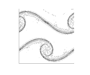
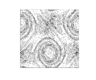
Figure 1. Vorticity contours for the double shear layer at time $t=6$ and $t=12$, $\gamma=0$.

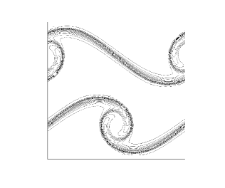
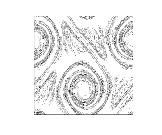
Figure 2. Vorticity contours for the double shear layer at time $t=6$ and $t=12$, $\gamma=10^{-2}$.

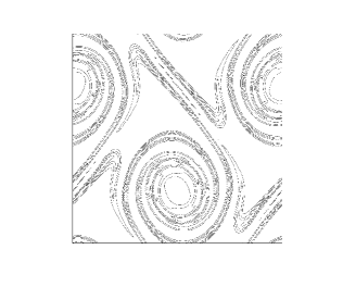
Figure 3. Vorticity contours for the double shear layer at time $t=6$ and $t=12$, $\gamma=10^{-1}$.

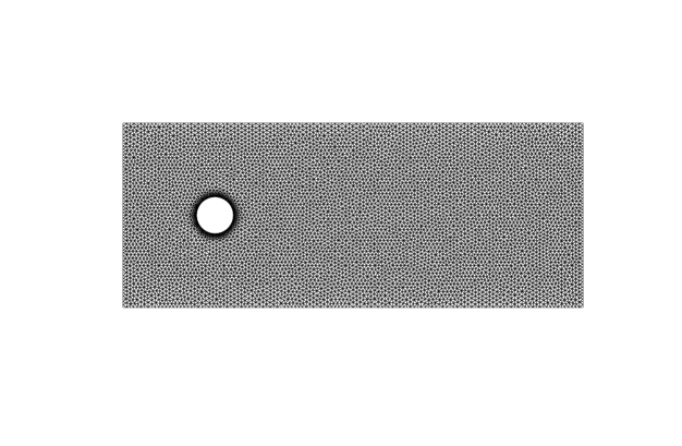
Figure 4. Mesh used for vortex shedding computation.

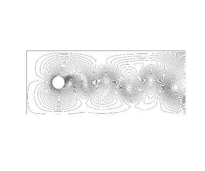
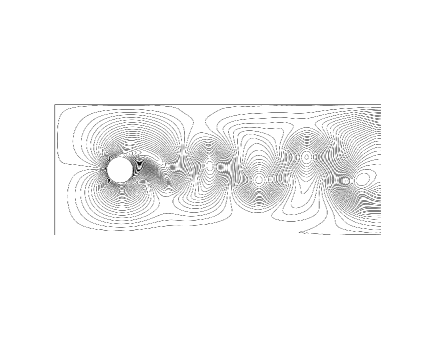
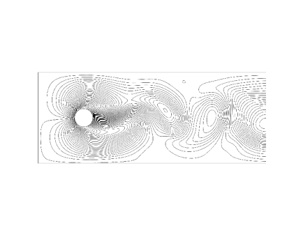
Figure 5. Relative streamlines at time $t=10$, $\gamma=0$,$\gamma=10^{-1}$, $\gamma=1$ from top.

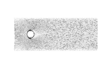
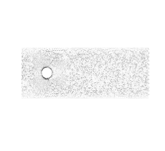
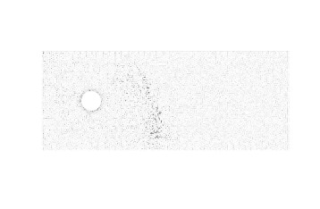
Figure 6. Velocities after 15, 20, and 30 timesteps, from top, $\mu=10^{-6}$, $\gamma=0$.

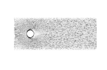
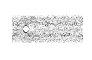
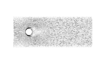
Figure 7. Velocities after 15, 20, and 30 timesteps from top, $\mu=10^{-6}$, $\gamma=10^{-1}$.

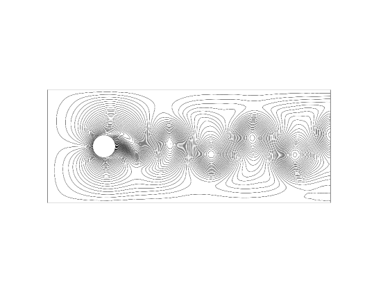
Figure 8. Relative streamlines at time $t=10$, $\mu=10^{-6}$, $\gamma=10^{-1}$.

References

- [1] H. Abidi and R. Danchin. Optimal bounds for the inviscid limit of Navier-Stokes equations. Asymptot. Anal., 38(1):35–46, 2004.
- [2] N. Ahmed, G. R. Barrenechea, E. Burman, J. Guzmán, A. Linke, and C. Merdon. A pressure-robust discretization of Oseen’s equation using stabilization in the vorticity equation. arXiv e-prints, page arXiv:2007.04012, July 2020.
- [3] C. Amrouche, C. Bernardi, M. Dauge, and V. Girault. Vector potentials in three-dimensional non-smooth domains. Math. Methods Appl. Sci., 21(9):823–864, 1998.
- [4] G. Barrenechea, E. Burman, and J. Guzman. Well-posedness and H(div)-conforming finite element approximation of a linearised model for inviscid incompressible flow. Mathematical Models and Methods in Applied Sciences, 1 2020.
- [5] H. Beirão da Veiga. On the Ladyzhenskaya-Smagorinsky turbulence model of the Navier-Stokes equations in smooth domains. The regularity problem. J. Eur. Math. Soc. (JEMS), 11(1):127–167, 2009.
- [6] H. Beirão da Veiga. Turbulence models, -fluid flows, and regularity of solutions. Commun. Pure Appl. Anal., 8(2):769–783, 2009.
- [7] J. B. Bell, P. Colella, and H. M. Glaz. A second-order projection method for the incompressible Navier-Stokes equations. J. Comput. Phys., 85(2):257–283, 1989.
- [8] R. Bellman. The stability of solutions of linear differential equations. Duke Math. J., 10(4):643–647, 12 1943.
- [9] J. P. Boris. More for LES: a brief historical perspective of MILES. In Implicit large eddy simulation, pages 9–38. Cambridge Univ. Press, Cambridge, 2007.
- [10] E. Burman. Robust error estimates for stabilized finite element approximations of the two dimensional Navier-Stokes’ equations at high Reynolds number. Comput. Methods Appl. Mech. Engrg., 288:2–23, 2015.
- [11] E. Burman, S. H. Christiansen, and P. Hansbo. Application of a minimal compatible element to incompressible and nearly incompressible continuum mechanics. Comput. Methods Appl. Mech. Engrg., 369:113224, 20, 2020.
- [12] E. Burman and M. A. Fernández. Continuous interior penalty finite element method for the time-dependent Navier-Stokes equations: space discretization and convergence. Numer. Math., 107(1):39–77, 2007.
- [13] E. Burman and A. Linke. Stabilized finite element schemes for incompressible flow using Scott-Vogelius elements. Appl. Numer. Math., 58(11):1704–1719, 2008.
- [14] S. H. Christiansen and K. Hu. Generalized finite element systems for smooth differential forms and Stokes’ problem. Numer. Math., 140(2):327–371, 2018.
- [15] M. Crouzeix and V. Thomée. The stability in and of the -projection onto finite element function spaces. Math. Comp., 48(178):521–532, 1987.
- [16] F. Demengel and G. Demengel. Functional spaces for the theory of elliptic partial differential equations. Universitext. Springer, London; EDP Sciences, Les Ulis, 2012. Translated from the 2007 French original by Reinie Erné.
- [17] D. A. Di Pietro and A. Ern. Mathematical aspects of discontinuous Galerkin methods, volume 69 of Mathématiques & Applications (Berlin) [Mathematics & Applications]. Springer, Heidelberg, 2012.
- [18] J. Droniou, R. Eymard, T. Gallouët, C. Guichard, and R. Herbin. The gradient discretisation method, volume 82 of Mathématiques & Applications (Berlin) [Mathematics & Applications]. Springer, Cham, 2018.
- [19] A. Ern and J.-L. Guermond. Theory and practice of finite elements, volume 159 of Applied Mathematical Sciences. Springer-Verlag, New York, 2004.
- [20] F. Fiedler and H. A. Panofsky. Atmospheric scales and spectral gaps. Bulletin of the American Meteorological Society, 51(12):1114–1119, 1970.
- [21] W. K. George and M. Tutkun. Mind the gap: a guideline for large eddy simulation. Philosophical Transactions of the Royal Society A: Mathematical, Physical and Engineering Sciences, 367(1899):2839–2847, 2009.
- [22] B. J. Geurts. Analysis of errors occurring in large eddy simulation. Philos. Trans. R. Soc. Lond. Ser. A Math. Phys. Eng. Sci., 367(1899):2873–2883, 2009. With supplementary material available online.
- [23] R. Glowinski and A. Marrocco. Sur l’approximation, par éléments finis d’ordre un, et la résolution, par pénalisation-dualité, d’une classe de problèmes de Dirichlet non linéaires. Rev. Française Automat. Informat. Recherche Opérationnelle Sér. Rouge Anal. Numér., 9(no. , no. R-2):41–76, 1975.
- [24] J.-L. Guermond and S. Prudhomme. On the construction of suitable solutions to the Navier-Stokes equations and questions regarding the definition of large eddy simulation. Phys. D, 207(1-2):64–78, 2005.
- [25] J. Guzmán and M. Neilan. inf-sup stable finite elements on barycentric refinements producing divergence-free approximations in arbitrary dimensions. SIAM J. Numer. Anal., 56(5):2826–2844, 2018.
- [26] P. Hansbo and A. Szepessy. A velocity-pressure streamline diffusion finite element method for the incompressible Navier-Stokes equations. Comput. Methods Appl. Mech. Engrg., 84(2):175–192, 1990.
- [27] J. Hoffman and C. Johnson. Computational turbulent incompressible flow, volume 4 of Applied Mathematics: Body and Soul. Springer, Berlin, 2007.
- [28] V. John. Finite element methods for incompressible flow problems, volume 51 of Springer Series in Computational Mathematics. Springer, Cham, 2016.
- [29] C. Johnson, R. Rannacher, and M. Boman. Numerics and hydrodynamic stability: toward error control in computational fluid dynamics. SIAM J. Numer. Anal., 32(4):1058–1079, 1995.
- [30] C. Johnson and J. Saranen. Streamline diffusion methods for the incompressible Euler and Navier-Stokes equations. Math. Comp., 47(175):1–18, 1986.
- [31] O. A. Ladyženskaja. Modifications of the Navier-Stokes equations for large gradients of the velocities. Zap. Naučn. Sem. Leningrad. Otdel. Mat. Inst. Steklov. (LOMI), 7:126–154, 1968.
- [32] W. Layton. Energy dissipation in the Smagorinsky model of turbulence. Appl. Math. Lett., 59:56–59, 2016.
- [33] J.-L. Lions. Quelques méthodes de résolution des problèmes aux limites non linéaires. Dunod; Gauthier-Villars, Paris, 1969.
- [34] J. Meyers, B. J. Geurts, and P. Sagaut. A computational error-assessment of central finite-volume discretizations in large-eddy simulation using a Smagorinsky model. J. Comput. Phys., 227(1):156–173, 2007.
- [35] A. Pouquet, U. Frisch, and J. P. Chollet. Turbulence with a spectral gap. The Physics of Fluids, 26(4):877–880, 1983.
- [36] J. Smagorinsky. General circulation experiments with the primitive equations.i.the basic experiment. Mon. Weather Rev., 91:99–164, 1963.
- [37] J. Smagorinsky. Some historical remarks on the use of nonlinear viscosities. In Large eddy simulation of complex engineering and geophysical flows, pages 3–36. Cambridge Univ. Press, New York, 1993.
- [38] E. R. Van Driest. On turbulent flow near a wall. Journal of the Aeronautical Sciences, 23(11):1007–1011, 1956.
- [39] J. Von Neumann and R. D. Richtmyer. A method for the numerical calculation of hydrodynamic shocks. J. Appl. Phys., 21:232–237, 1950.
- [40] J. Weinstock. A Theory of Gaps in the Turbulence Spectra of Stably Stratified Shear Flows. Journal of the Atmospheric Sciences, 37(7):1542–1549, 07 1980.
- [41] S. Zhang. On the P1 Powell-Sabin divergence-free finite element for the Stokes equations. J. Comput. Math., 26(3):456–470, 2008.