Mapping stellar surfaces
I: Degeneracies in the rotational light curve problem

Abstract

Thanks to missions like Kepler and TESS, we now have access to tens of thousands of high precision, fast cadence, and long baseline stellar photometric observations. In principle, these light curves encode a vast amount of information about stellar variability and, in particular, about the distribution of starspots and other features on their surfaces. Unfortunately, the problem of inferring stellar surface properties from a rotational light curve is famously ill-posed, as it often does not admit a unique solution. Inference about the number, size, contrast, and location of spots can therefore depend very strongly on the assumptions of the model, the regularization scheme, or the prior. The goal of this paper is twofold: (1) to explore the various degeneracies affecting the stellar light curve “inversion” problem and their effect on what can and cannot be learned from a stellar surface given unresolved photometric measurements; and (2) to motivate ensemble analyses of the light curves of many stars at once as a powerful data-driven alternative to common priors adopted in the literature. We further derive novel results on the dependence of the null space on stellar inclination and limb darkening and show that single-band photometric measurements cannot uniquely constrain quantities like the total spot coverage without the use of strong priors. This is the first in a series of papers devoted to the development of novel algorithms and tools for the analysis of stellar light curves and spectral time series, with the explicit goal of enabling statistically robust inference about their surface properties.

open-source figures ; equation unit tests: 5 passed , 0 failed

1 Introduction

The advent of space-based precision photometry with missions such as Kepler (Borucki et al., 2010) and TESS (Ricker et al., 2015) has led to a renewed interest in the modeling of stellar light curves, and, in particular, in understanding what these light curves can tell us about the surfaces of stars across the HR diagram. One of the dominant sources of stellar light curve variability is the modulation caused by starspots rotating in and out of view. Dark spots arise due to the suppression of convection in regions of intense magnetic field, resulting in a locally cooler (and hence darker) photosphere. Bright spots can similarly arise in the photosphere as faculae or in the chromosphere as plages, and are also magnetically driven (e.g., Berdyugina, 2005). Constraining the sizes, contrasts, locations, and number of spots on stars can therefore reveal information about stellar magnetic activity, stellar interior structure, and how these quantities vary across spectral type and over time (e.g., Garraffo et al., 2018). A detailed understanding of the stellar surface is also crucial to mitigating systematics in the radial velocity search for exoplanets (e.g., Lanza et al., 2011) and in the spectroscopic characterization of their atmospheres (e.g., Rackham et al., 2018).

To date, most studies aimed at inferring stellar surface properties from light curves follow one of two broad approaches. The first is to model the stellar surface as a collection of one or more discrete, circular, uniform contrast dark or bright spots on a uniform intensity photosphere. The advantage of this approach is that the light curve can be computed efficiently and in some cases even analytically (e.g., Davenport et al., 2015; Morris et al., 2017; Morris, 2020a). The second approach is to discretize the surface at some resolution and compute the emergent flux as a weighted sum of the visible pixel intensities. This approach is more flexible, since it is not limited to surfaces composed of distinct circular spots (e.g., Harmon & Crews, 2000; Roettenbacher et al., 2017). Both approaches rely on an explicit forward model, a prescription for how to generate data given a set of parameters. In most cases, however, we are interested in the inverse problem: constraining the parameters given data. Unfortunately, the inverse problem is not only difficult—as it requires a large number of forward model evaluations to find the parameter values that are most consistent with the data—but also formally ill-posed. While the mapping from a stellar surface to a light curve (the forward problem) is unique, the mapping from a light curve to a surface (the inverse problem) is not: given any light curve, there exist an infinite number of surfaces that could have generated it. These degeneracies are illustrated in Figure 1, where six synthetic stellar surfaces are shown (rows) at twelve different phases (columns), all at an inclination $I=60^{\circ}$. Each surface consists of a different number of dark spots on a brighter, heterogeneous background.

Figure 1: The fundamental limitations of the mapping problem. Each row corresponds to a stellar surface with a different number of dark spots seen at various phases at an inclination $I=60^{\circ}$; all images are shown on the same color scale. The bottom panel shows the light curves of each of these stars. All six light curves are indistinguishable from each other, even at infinite signal to noise. See text for details.   

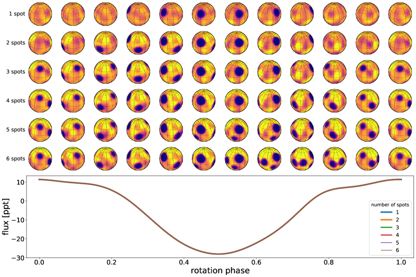
While the stellar surfaces are all distinct, containing between one (top) and six (bottom) large dark spots, their rotational light curves are identical (lower panel). This is true even in the absence of measurement error: the mapping from a stellar surface to its rotational light curve is so degenerate that there exist an infinite number of solutions to the inverse problem. This fact has been pointed out recently in different contexts (e.g., Cowan et al., 2013; Rauscher et al., 2018; Sandford & Kipping, 2019; Luger et al., 2019; Basri & Shah, 2020), but it dates back at least to Russell (1906), who demonstrated it by expanding the surface intensity of a celestial body in terms of spherical harmonics (see Figure 2). Russell (1906) showed that many of the modes comprising the intensity profile of a spherical object are in the null space, the set of surface features that have identically zero effect on the light curve. In fact, as we will show in §2, the vast majority of the modes are in the null space for rotational light curves of stars. This is what allows us to construct pathological scenarios like that shown in Figure 1, where the light curve could be explained by any number of spots atop a heterogeneous bright background.

Stellar mapping studies tackle these degeneracies in different ways, but it usually comes down to a choice of prior: when the data is not sufficiently informative, assumptions—either implicit or explicit—are needed to discriminate between competing solutions. In discrete spot models like the ones discussed above, the degeneracy-breaking prior is (typically) the assumption that the spots must be circular, have uniform contrast, and sit atop an otherwise uniform photosphere. In gridded stellar surface models, it is common to assume a regularization prior such as the maximum entropy penalty (e.g., Vogt et al., 1987), which typically favors solutions with the fewest number of dark pixels (usually referred to as the “simplest” solution).

While these assumptions may be approximately valid in some cases, it is important to bear in mind that because of the light curve degeneracies discussed above, most of the information about the stellar surface usually comes from the modeling assumptions, so it is very important to get these assumptions right. In general, starspots are not circular and do not have uniform contrast throughout; nor do spots always arrange themselves in the highest entropy configuration. The amount of bias introduced by these assumptions will in general vary, but in principle it could be quite significant.

The goal of this paper is to explore the degeneracies at play in the stellar surface mapping problem from a theoretical standpoint. We will focus in particular on two sources of degeneracies: the null space intrinsic to the mapping from a two-dimensional surface to a one-dimensional light curve (§2) and the degeneracy due to the unknowability of the true normalization in single-band photometry (§3). Within each section we will discuss ways to either break these degeneracies or marginalize over unknowable quantities. We will focus in particular on the power of ensemble analyses: the joint analysis of many light curves of statistically “similar” stars. We will show that even though individual light curves are not very constraining, light curves of many stars observed at different inclinations can uniquely constrain certain properties of the surfaces of those stars. This idea was recently explored to some extent in Morris (2020b), who used ensemble analyses to derive constraints on spot coverage areas as a function of stellar age. However, one of the main conclusions of the present paper is that quantities like the total spot coverage and the total number of spots are not direct observables in single-band photometry. Instead, any constraints placed on these quantities, even in the context of ensemble analyses, are usually driven by the choice of prior and other assumptions.

The present paper is also similar to Walkowicz et al. (2013) and Basri & Shah (2020), who explored the information content of stellar light curves from a large set of simulated spotted stellar surfaces. While our paper is largely complementary to that work, we instead approach the information content problem from a theoretical—as opposed to empirical—point of view. The present paper is the first in a series dedicated to the development of techniques to perform robust inference about stellar surfaces from unresolved photometric and spectroscopic measurements. The results of this paper serve as the starting point for the development of an interpretable Gaussian process for the ensemble analysis of stellar light curves, which is the subject of (Luger et al. 2021, hereafter Paper II, ).

All of the figures in this paper were auto-generated using the Azure Pipelines continuous integration (CI) service. Icons next to each of the figures   link to the exact script used to generate them to ensure the reproducibility of our results. In this paper we also introduce the concept of equation “unit tests”: pytest-compatible test scripts associated with the principal equations that pass (fail) if the equation is correct (wrong), in which case a clickable   () is shown next to the equation label. In most cases, the validity of an equation is gauged by comparison to a numerical solution. Like the figure scripts, the equation unit tests are run on Azure Pipelines upon every commit of the code.

2 The null space

In this section, we define the concept of the null space and present some demonstrations showing how it can affect inferences about stellar surfaces. For simplicity, we assume we know quantities like the stellar inclination, rotation period, and limb darkening coefficients exactly, and we assume the stellar surface does not vary in time (i.e., spots do not evolve and the star rotates as a rigid body). Because of these assumptions, our constraints on the information content of light curves should be viewed as strict upper limits.

We also present some examples of how the degeneracies due to the null space can be tackled. While our examples below may appear somewhat idealized, at the end of this section we discuss how our ideas generalize to more realistic scenario; we also revisit these assumptions in §4.3. This is also a topic that we discuss in much more detail in Paper II.

Figure 2: The real spherical harmonics in the polar frame ($\hat{\mathbf{x}}$ points to the right, $\hat{\mathbf{y}}$ points up, and $\hat{\mathbf{z}}$ points out of the page) up to $l=5$. Dark colors correspond to negative intensity and bright colors to positive intensity; rows correspond to the degree $l$ and columns to the order $m$. The set of all spherical harmonics forms a complete, orthogonal basis on the sphere.   

2.1 Rank of the flux operator

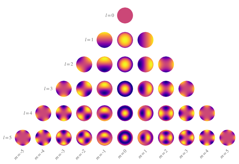
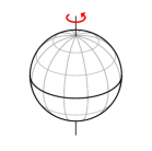
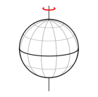
In general, inferring all of the properties of a stellar surface from its light curve alone is not only difficult, but formally impossible. To understand why, consider an expansion of the stellar surface intensity in the spherical harmonic basis out to arbitrary order (see Figure 2). Assuming (for the moment) that the star rotates about an axis that points up along the page, the observed light curve may be expressed as a weighted sum of the disk-integrated intensity of each of the spherical harmonics as they rotate about that same axis (Luger et al., 2019). However, not all spherical harmonics will contribute to the full light curve, as many (in fact, most) of the spherical harmonics are perfectly antisymmetric about the equator. This is the case for the $l=1$, $m=-1$ harmonic, which integrates to zero regardless of the phase at which it is viewed. The same is true, in fact, for all other harmonics of order $m=-1$ and (perhaps less obviously) for all harmonics with odd $l=3,5,7,...$ Furthermore, there exist many linear combinations of spherical harmonics that similarly integrate to zero at all rotational phases. Together, these modes constitute the null space of the problem: the set of modes on the surface that do not contribute to the observed light curve and therefore cannot be probed from photometry.

For rotational light curves, the vast majority of the surface modes lie in the null space. To show this, we will make use of the fact that we can express the vector of $K$ observed fluxes $\mathbf{f}$ (i.e., the light curve) as a linear operation on the vector of $N$ spherical harmonic coefficients $\mathbf{y}$ (Luger et al., 2019):

$$\mathbf{f}=\mathbf{1}+\boldsymbol{\mathcal{A}}\,\mathbf{y}\hskip 0.0pt,$$ (1)

where $\boldsymbol{\mathcal{A}}$ is the $(K\times N)$ design matrix of the transformation, whose columns describe how each of the $N$ components in the spherical harmonic basis contribute to each of the $K$ points in the light curve. Even though we are explicitly choosing the spherical harmonics as the basis in which we describe the stellar surface, Equation (1) is quite general and applies to any basis that is linearly related to the flux. For instance, $\mathbf{y}$ could instead describe the intensity deficits in each of the $N$ pixels of a gridded stellar surface, in which case $\boldsymbol{\mathcal{A}}$ would be the matrix of pixel visibilities that describe how to sum each of the pixels to obtain the observed light curve.

The size of the null space is called the nullity, and it is equal to $N-R$, where $N$ is once again the number of coefficients describing the stellar surface and $R$ is the rank of the flux operator $\boldsymbol{\mathcal{A}}$. The rank $R$ is the number of linearly independent columns in $\boldsymbol{\mathcal{A}}$, which can be computed numerically using any standard linear algebra package. It is equal to the number of independent components that can be measured given an observation of $\mathbf{f}$.

Figure 3: Rank and nullity of the flux operator. The orange curve shows the number of spherical harmonic coefficients required to fully describe a stellar surface up to a given spherical harmonic degree (bottom axis) or, equivalently, up to an effective surface resolution (top axis). The blue curve shows the rank of the flux operator, corresponding to the maximum number of independent degrees of freedom that can be constrained from a light curve. The size of the null space (the nullity) is the difference between the two curves.   

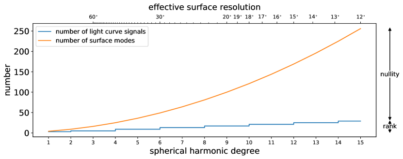
Figure 3 shows the rank and nullity of the flux operator as a function of the resolution of the surface map (quantified as the spherical harmonic degree $l$ of the expansion). The orange curve is the number of spherical harmonic coefficients needed to represent a surface map up to degree $l$, and is equal to $N=(l+1)^{2}$. The blue line shows the rank of the flux operator $\boldsymbol{\mathcal{A}}$ as a function of $l$, which scales as $R\approx 2l+1$. The nullity is simply the difference between $N$ and $R$.

The most striking feature in Figure 3 is how quickly the two curves diverge as $l$ increases. What this means for the mapping problem is that the number of surface modes—the total information needed to represent a surface map at some resolution—grows much more quickly than the number of independent degrees of freedom in the light curve. At all but the lowest resolutions, there are always more features in the null space than components one can measure in the light curve, a difference that grows quadratically with $l$. This means that although a light curve can tell us some information about a stellar surface on very large scales, the amount of information it tells us quickly decreases for smaller scales and all but vanishes for the smallest surface features.

It is also worth noting the piecewise nature of the rank as a function of $l$: increasing the degree of the expansion from even $l$ to odd $l$ does not increase the rank of the flux operator. Put another way, odd spherical harmonic modes with $l>1$ are always in the null space of the light curve. We will return to this point below.

2.2 Decomposition of the flux operator

In Appendix A we show that it is straightforward to construct linear operators $\mathbf{P}$ and $\mathbf{N}$ from the design matrix $\boldsymbol{\mathcal{A}}$ such that

$$\mathbf{y}_{\bullet} =\mathbf{P}\,\mathbf{y}$$ (2)

is the component of the surface map in the preimage and

$$\mathbf{y}_{\circ} =\mathbf{N}\,\mathbf{y}$$ (3)

is the component of the map in the null space. The preimage operator $\mathbf{P}$ transforms a vector $\mathbf{y}$ in the surface map basis in such a way that it preserves the information in $\mathbf{y}$ that gets mapped onto the light curve $\mathbf{f}$ via $\boldsymbol{\mathcal{A}}$ (the preimage) and discards the rest. The null space operator $\mathbf{N}$ does the opposite: it preserves only the information in $\mathbf{y}$ that gets mapped onto the zero vector via $\boldsymbol{\mathcal{A}}$ (the null space). In other words, the $\mathbf{P}$ and $\mathbf{N}$ operators reveal the components of the surface map that contribute to the light curve ($\mathbf{y}_{\bullet}$) and the components that don’t ($\mathbf{y}_{\circ}$). The vector $\mathbf{y}_{\bullet}$ represents all the information that can be learned from a stellar light curve, while $\mathbf{y}_{\circ}$ represents all the information that cannot.

Figure 4: Decomposition of a surface map (left column) into its preimage (center) and null space (right) components for different surfaces, and their corresponding contributions to the rotational light curve. The preimage is the set of surfaces modes that map onto the light curve; the null space is the set of modes that do not. An inclination of $60^{\circ}$ is assumed when computing the flux. The vast majority of surface modes are in the null space of the light curve problem and therefore do not contribute to the observed flux.   

Figure 5: Same as Figure 4, but for a stellar inclination of $85^{\circ}$. As the stellar rotation vector becomes perpendicular to the line of sight, it becomes more difficult to constrain latitudinal information.   

It is instructive to visualize these components in an actual surface mapping exercise. Figure 4 shows the decomposition of four hypothetical surfaces (left column) into preimage (center) and null space (right) components under the flux operator $\boldsymbol{\mathcal{A}}$, which we compute for definiteness at an inclination of $I=60^{\circ}$ over a full rotation. Surfaces are shown in an equal-area Mollweide projection alongside the corresponding light curves. Note that both the true map and its associated light curve are simply equal to the sum of the preimage and null space components (Appendix A). As expected, all of the information in the light curve comes from the preimage, and the null space contributes exactly zero flux at all phases. However, most of the information about the surface is stuck in the null space!

In the top row of the figure, corresponding to a surface with a single large spot, it is clear that the light curve contains information about the presence of the spot at roughly the correct longitude and latitude. There are additional artefacts across the stellar surface, and the exact shape of the spot is not well constrained by the data; these issues, however, can easily be resolved with a circular spot prior.

The degeneracies of the mapping problem are much more apparent in the second and third rows, corresponding to surfaces with many, smaller spots. The locations, sizes, and the very existence of most of the spots are simply not encoded in the light curve. Even with an extremely restrictive prior, it may be difficult—if not impossible—to learn the properties of the spots from the individual light curves.

The final row corresponds to a surface with much higher resolution features; this example highlights how the information content of light curves all but vanishes at small scales. Virtually all of the spatial information at the scales of interest is in the null space.

2.3 Implications for inference

The model mapping spherical harmonic coefficients to observed fluxes described in the preceding sections is linear, so we might expect that we could fit for the spherical harmonics using linear least-squares

$$\hat{\mathbf{y}} \stackrel{{\scriptstyle?}}{{=}}\left(\boldsymbol{\mathcal{A}}^{\top}\,\boldsymbol{\mathcal{A}}\right)^{-1}\,\boldsymbol{\mathcal{A}}^{\top}\,\left(\mathbf{f}-\mathbf{1}\right)\hskip 0.0pt.$$ (4)

But, since the flux operator $\boldsymbol{\mathcal{A}}$ is low-rank, the model is underdetermined, so the above operation is not defined and, equivalently, the Fisher information matrix

$$\boldsymbol{\mathcal{I}}(\mathbf{y}) =\frac{1}{\sigma_{f}^{2}}\,\boldsymbol{\mathcal{A}}^{\top}\,\boldsymbol{\mathcal{A}}$$ (5)

is singular. In Equation (5), $\sigma_{f}$ is the flux measurement uncertainty. There exist many methods and procedures for linear regression for underdetermined models, but all solutions amount to imposing stronger assumptions about the model in order to break the degeneracies.

One standard method is regularized least squares, in which Equation (4) becomes

$$\hat{\mathbf{y}}_{\lambda} \equiv\left(\boldsymbol{\mathcal{A}}^{\top}\,\boldsymbol{\mathcal{A}}+\lambda\,\mathbf{I}\right)^{-1}\,\boldsymbol{\mathcal{A}}^{\top}\,\left(\mathbf{f}-\mathbf{1}\right)$$ (6)

where $\mathbf{I}$ is the identity matrix and $\lambda$ is a parameter controlling the strength of the regularization. In a Bayesian context, this can be interpreted as placing a Gaussian prior with variance $\sigma_{0}^{2}=\nicefrac{{\sigma_{f}^{2}}}{{\lambda}}$ on the spherical harmonic coefficients.

In the limit of infinitesimal regularization, it can be demonstrated (see Hogg & Villar, 2021, for example) that

$$\lim_{\lambda\rightarrow 0_{+}}\hat{\mathbf{y}}_{\lambda} =\mathbf{y}_{\bullet}\hskip 0.0pt.$$  (7)

In this sense, $\mathbf{y}_{\bullet}$ represents our knowledge about the surface of a star after an observation if we have no prior information whatsoever on $\mathbf{y}$. Any other information about the surface is entirely driven by our assumptions.

Equation (7) is the solution to the surface map we would obtain if we knew nothing about the stellar surface before analyzing the light curve. In practice, this is never really the case. For instance, we know that stellar surfaces must have non-negative intensities everywhere. While this may seem like a trivial prior, non-negativity can be a powerful degeneracy-breaking constraint (e.g., Fienup, 1982). Moreover, we know that stellar surfaces usually consist of localized features; under an appropriate compactness prior, solutions like the preimage in the bottom row of Figure 4 (for example) could be confidently ruled out.

The effect of different modeling assumptions on the structure and size of the null space is beyond the scope of this paper. In general, this is a particularly difficult question to address because non-Gaussian priors on the surface map break the linearity of the problem. While compactness constraints (like the assumption of a small number of discrete circular spots) can break many of the degeneracies discussed here, simulation-based arguments show that it is still not possible to uniquely constrain their number, locations, or sizes from individual light curves (Basri & Shah, 2020).

2.4 Dependence on inclination

Figure 5 shows the same decomposition of stellar surfaces into what can be learned (the preimage) and what cannot be learned (the null space) from a light cuve, but this time for stars viewed at an inclination $I=85^{\circ}$. Interestingly, the structure of the null space is somewhat different; in particular, features in the preimage are latitudinally smeared. This issue is well known (e.g., Cowan et al., 2009; Basri & Shah, 2020), and any information about which hemisphere a feature is in formally vanishes as $I\rightarrow 90^{\circ}$.

Instead of lamenting the difficulties of constraining stellar surface features at near-edge-on orientations, let us focus on the fact that the null space is a function of inclination. A useful property of the spherical harmonics is that a rotation operation on any component in the basis can only change the order $m$ of the harmonic; the degree $l$ is constant under rotation. In other words, rotating any of the spherical harmonics in Figure 2 about an arbitrary axis simply yields a weighted sum of the spherical harmonics along its row. This means that changing the inclination of the star—which changes the axis of rotation in the observer’s frame—simply changes the weighting of modes that give rise to certain signals in the light curve. This, in turn, results in the dependence of the null space on inclination.

To better understand this effect, let us define the quantity

$$S\equiv 1-\lim_{\lambda\rightarrow 0_{+}}\mathrm{diag}\left(\lambda\left(\boldsymbol{\mathcal{A}}^{\top}\,\boldsymbol{\mathcal{A}}+\lambda\,\mathbf{I}\right)^{-1}\right)\hskip 0.0pt,$$ (8)

which we will refer to as the variance reduction  of the coefficients $\mathbf{y}$ characterizing the stellar surface. Note that in a Bayesian context, this is equivalent to the posterior shrinkage

$$S=1-\lim\limits_{\sigma_{0}^{2}\rightarrow\infty}\frac{\sigma^{2}}{\sigma_{0}^{2}}\hskip 0.0pt,$$ (9)

where $\sigma_{0}^{2}$ is the prior variance and $\sigma^{2}$ is the posterior variance on a particular surface mode we are trying to constrain (see, e.g., Betancourt, 2018).

The variance reduction is a dimensionless quantity describing how informative a measurement is about a given mode on the surface in the limit of infinite signal-to-noise ratio (SNR) and is independent of what the stellar surface actually looks like. If, at infinite SNR and with no regularization (or, in a Bayesian context, a completely uninformative prior), a particular mode can be learned exactly from a dataset, the variance reduction is defined to be unity. Conversely, if the data is completely unconstraining of that mode (i.e., it is entirely in the null space), $S$ will tend to zero.

Figure 6: The variance reduction as a function of spherical harmonic degree $l$ given a single observation of a star at a random inclination (thin blue curves). The mean variance reduction is shown as the thicker curve. The information content of light curves tends to zero as $l$ increases, and odd $l>1$ modes are in the null space at all inclinations.   

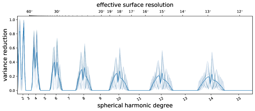
Figure 6 shows the variance reduction $S$ given a single observation of a star at a random inclination. Each thin blue curve corresponds to a particular draw from an isotropic inclination distribution; the thick blue curve is the average over 300 trials. For some of the low-degree modes, $S$ is relatively high: it is fairly easy to constrain the dipole moment from a light curve, as this is usually the dominant sinusoidal signal. However, as the degree $l$ increases, $S$ decreases dramatically: at $l=14$, corresponding to features on scales of roughly $13^{\circ}$, the light curve can only tell us about $\sim 10\%$ of the total information about what the surface looks like. As $l$ increases further, $S$ tends to zero. Another important feature of $S$, which we hinted at above, is that it is exactly zero for all odd-degree modes above $l=1$. This is a well-known fact: all odd spherical harmonics other than the dipole are in the null space regardless of inclination (e.g., Luger et al., 2019). In other words, these spherical harmonics are perfectly antisymmetric in projection over the unit disk when viewed from any orientation. Absent structure to break these symmetries (see below), we simply cannot learn anything about these modes from stellar light curves. If we average over $S$ for all modes up to $l=15$, we find that a single light curve measurement can only tell us $\sim 9\%$ of the information about the surface on those scales.

Fortunately, however, there is quite a bit of scatter in $S$ for different values of the stellar inclination. As we will see, we can use this dependence of the null space on inclination to our advantage. If we could observe a star from many different vantage points, we would be able to break many of the degeneracies at play, since we would get different constraints on the amplitude of each mode when viewed at different inclinations. This, of course, is not possible (at least not yet!). But what we can do is observe many similar stars, each viewed at a different (random) inclination, and attempt to learn something about the properties of the ensemble of stars as a whole. In the following section, we explore the role of ensemble analyses in breaking the degeneracies of the mapping problem in more detail.

2.5 Ensemble analyses

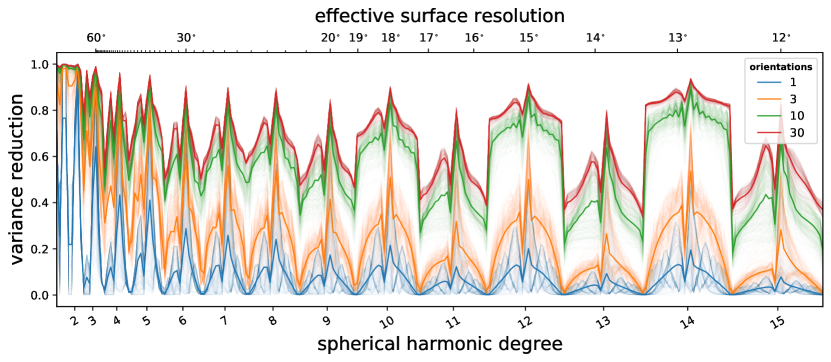
In an ensemble analysis, we assume we observe the lightcurves of many stars that are “similar” in some statistical sense. As a thought experiment, let us consider an extreme version of ensemble analysis in which all the stars in our sample happen to have identical surfaces. We will still assume they are oriented at random inclinations, as we would expect for field stars. Figure 7 shows the variance reduction curves for this hypothetical scenario, assuming we have access to light curves of 1 (blue), 3 (orange), 10 (green) and 30 (red) identical stars viewed at random inclinations.

Figure 7: Similar to Figure 6, but assuming the observer can measure the light curves of 1 (blue), 3 (orange), 10 (green), and 30 (red) identical stars–(same surface map, same rotational phase–but viewed at random orientations. As we saw in Figure 6, the information content in the light curve of a star observed from a single vantage point approaches zero as $l$ increases. However, observing many identical stars from different vantage points allows one to recover nearly all of the information in the even spherical harmonic modes. This is why ensemble analyses of many similar stars at different inclinations allows us to infer their surface properties.   

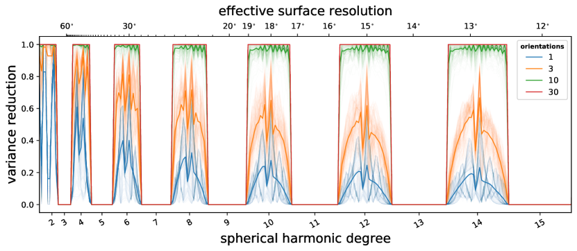
The addition of light curve measurements at different orientations increases the variance reduction at all even spherical harmonic degrees (the odd degrees, as we mentioned above, are always invisible). Note that since we are in the limit of infinite SNR, the fact that we have more light curves (i.e., more data) is irrelevant: the increase in the variance reduction is instead due to the fact that our observations from different vantage points broke some degeneracies in the problem. This is a consequence of the fact we mentioned in the previous section: the null space (for the even modes) is a strong function of the inclination.

If we average over all modes, we obtain an average $S$ of $\sim 24\%$ for $l\leq 15$ when our sample size is 3 (orange curves): we have more than doubled the information content of our observations. If we further increase our sample size to 10 (green curves), the variance reduction approaches $100\%$ for all even $l\leq 15$ modes, effectively saturating for a sample size of 30 (red curves). Thus, if we were able to measure light curves of identical stars from many different inclinations, the null space would consist only of the odd modes. In the limit of a large number of light curves, and assuming all stars in the sample have identical surfaces, ensemble analyses can tell us up to half of all the information about the stellar surfaces.

Figure 8: Same as Figures 4 and 5,  but assuming we can measure the light curves of these stars from many different inclinations. In this limit, the information content of our data approaches $50\%$ of the spatial information about the surface.   

To understand what we can learn about the surfaces in this limit, let us return to the stellar surfaces we considered in Figures 4 and 5. Figure 8 shows the same decomposition of these surfaces into preimage and null space, but this time assuming we measure the light curves of these stars from many different random inclinations. As expected, the partition of information between the preimage and the nullspace is about $50{-}50$. Because spots are compact features, they are necessarily made up of a continuum of spherical harmonic modes spanning many different values of $l$: they can therefore be seen in both the even modes (the preimage) and the odd modes (the null space). The absence of information about the odd modes therefore does not affect our ability to infer the shape and location of the features on the surface. Interestingly, however, the symmetries at play require spots to be paired with antipodal dark mirror images in the preimage, and with bright ones in the null space (which sum to perfectly cancel out in the true map). Thus, there are still degeneracies in this very idealized ensemble problem, but they are much easier to break with a suitable choice of prior. For instance, in the single spot case (top row), the “ghost” image in the southern hemisphere is surrounded by a bright ring (whose effect is to cancel out its contribution to the flux); either a compactness prior or a prior that enforces uniformity in the background could easily penalize that feature in the fit. This may be much harder to do for surfaces like that shown in the second row, but we can still (in principle) learn about the size, shape, and latitude (if not the number) of starspots from the light curves.

There are several practical reasons why this kind of ensemble analysis may be very difficult (but not impossible!) in practice. Before we address those, let us consider an important effect that we have not addressed thus far in this paper: limb darkening.

2.6 The effect of limb darkening

Figure 9: Same as Figure 7, but for limb-darkened stars with quadratic coefficients $u_{1}=0.5$ and $u_{2}=0.25$. Odd modes can now be probed, at the expense of the even modes.   

Typically, the shallower the angle between the line of sight and the stellar surface normal, the higher up in the stellar atmosphere optical depth unity is reached. At optical wavelengths, lines of sight directed toward the limb of the star therefore probe cooler temperatures, resulting in the well-known effect of limb darkening. Features close to the limb of the star therefore contribute less to the total outgoing flux, and this must be accounted for when computing the effect of a rotating starspot on the light curve. Limb darkening is often parametrized as a low-order polynomial in the cosine of the line of sight angle (Kopal, 1950).

To understand how limb darkening affects our ability to infer surface properties from stellar light curves, let us repeat the experiment from the previous section, this time with moderate quadratic limb darkening (with coefficients $u_{1}=0.5$ and $u_{2}=0.25$, although our conclusions do not qualitatively change for different values). The top panel of Figure 9 shows the variance reduction plot (same as Figure 7, but this time accounting for limb darkening). Interestingly, there is no longer a clean division of the null space between even and odd modes in the limit of a large number of light curves. This is because limb darkening effectively lifts odd modes out of the null space, at the expense of the even modes. While no coefficient lies entirely in the null space ($S=0$) when limb darkening is present, no coefficient can be uniquely inferred ($S=1$), either. This can be understood by noting that a polynomial limb darkening law can be written exactly as a linear combination of the $m=0$ spherical harmonics up to a degree equal to the order of the limb darkening (Luger et al., 2019; Agol et al., 2020, in this case, $l=2$;). Since the limb darkening operation is a (multiplicative) downweighting of the surface intensity, the map seen by the observer is just the product of the spherical harmonic representation of the surface ($\mathbf{y}$) and the spherical harmonic representation of the limb darkening profile. And since spherical harmonics are just polynomials on the surface of the sphere, the product of spherical harmonics of degree $l_{1}$ and $l_{2}$ is a spherical harmonic of degree $l_{1}+l_{2}$. This means that the linear limb darkening component ($l=1$) effectively raises the degree of all spherical harmonic coefficients of the surface map by one. This has the effect of reversing the null space: under only linear limb darkening, it is the even modes that would be in the null space. However, the quadratic limb darkening term ($l=2$) raises the degree of all spherical harmonics by two, so its presence ensures that the even modes can still be probed to some extent. In reality, the true limb darkening profile of a stellar surface is more complicated than a two-parameter quadratic model can capture; but one may still expand it as an arbitrary order polynomial, in which case the argument still applies—limb darkening mixes the null space and the preimage in a nontrivial way. The fact that no coefficient can be determined uniquely—i.e., there are perfect degeneracies involving all modes on the surface—could make it more difficult in practice to perform ensemble analyses on limb-darkened stars.

Figure 10: Same as Figure 9, but allowing for a 10% variation in the limb darkening coefficients $u_{1}$ and $u_{2}$ across different observations. For $\gtrsim 30$ light curves, there is virtually no null space up to at least $l_{\mathrm{max}}=15$.   

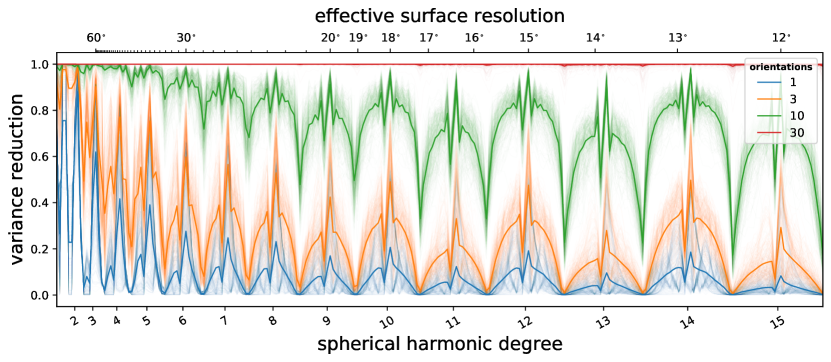
In reality, it is unlikely that all stars in a given ensemble will have exactly the same limb darkening coefficients, however “similar” the stars may be. Figure 10 shows the same variance reduction plot as Figure 9, but for the case where each star has coefficients $u_{1}=0.5\pm 0.05$ and $u_{2}=0.25\pm 0.025$; i.e., we add a scatter of 10% in the value of these coefficients. The plot shows the variance reduction in the hypothetical case where we know the coefficients for each star exactly. Now, as the size of the ensemble increases, the variance reduction approaches unity for all spherical harmonic modes. In the same way that the null space is a strong function of the inclination, allowing us to chip away at it with observations at different inclinations, the null space is also a strong function of the limb darkening law. Even a small amount of variance in the coefficients is sufficient to constrain all surface modes exactly (in the limit of infinite SNR and a large number of light curves).

In practice, of course, we will never know the limb darkening coefficients exactly. In the next section, we will revisit this and other assumptions we made above in a more sober light.

2.7 A reality check

There are three major points that make the kind of ensemble analyses discussed above difficult in practice. First, and perhaps most obviously, stars are not identical, no matter how “similar” we think they may be. Even stars of the same spectral type, age, and metallicity will in general have different configurations of spots on their surfaces. When we perform an ensemble analysis on the light curves of a heterogeneous group of stars, we are learning something about the distribution of surface properties across all the stars in the sample—not the surface properties of any individual star. What exactly we can learn in this case is not immediately obvious, and requires a detailed investigation. This is the subject of the next paper in this series (Paper II), where we show that, armed with a good model, we can learn a lot about the distribution of starspot properties of a heterogenous group of stellar light curves.

The second point is that while observing many similar stars at different inclinations can greatly help us learn about their surfaces from a statistical standpoint, our analysis above assumed we knew what the values of the individual inclinations were. In practice, this will usually not be the case. While we may have good priors for some stars (from spectroscopic $v\sin I$ measurements, or from the assumption that transiting exoplanet hosts are likely to have inclinations close to $I=90^{\circ}$), for the vast majority of field stars we won’t know much a priori. Since the inclination is typically degenerate with the spot latitude (e.g., Walkowicz et al., 2013), this decreases the constraining power of ensemble analyses. However, as we show in Paper II, there is still enough information in ensembles of $\gtrsim 50$ light curves to independently constrain the spot latitudes and the individual stellar inclinations.

The final point concerns limb darkening, which also has a strong effect on the structure of the null space. While limb darkening can help us in the same way as the inclination, in practice it is likely to be more of a problem, since the use of incorrect limb darkening coefficients can lead to bias in the spot properties when doing inference. It is therefore extremely important to use reliable limb darkening models when doing ensemble analyses; we also explore this in Paper II.

3 The normalization degeneracy

Thus far we have focused our discussion on theoretical aspects concerning what can and cannot be learned from disk-integrated photometric measurements of stellar surfaces. In this section, we discuss an important degeneracy introduced by how we actually measure stellar light curves, which we will refer to as the normalization degeneracy. This degeneracy has been pointed out before (e.g., Basri, 2018), but it is useful to revisit and build on it here.

3.1 A fundamental issue of units

To understand the normalization degeneracy, consider how we might go about simulating a stellar surface. We might add a dark spot somewhere on the surface, either by expanding it in spherical harmonics or by gridding up the stellar surface and setting the intensity of pixels within the spot to a low value. To compute the light curve, we integrate over the projected disk at each point in time. The resulting light curve will have strange units, so we might then divide by the integral of the background intensity over the unit disk, so that we are now in what we will call fractional units: the flux as a fraction of the flux we would measure if the star had no spots on it.

Figure 11: An example of the normalization problem. Top: Consider a star with a single equatorial spot of contrast $c$ viewed at a certain inclination. The total flux (in some units) as a function of time is shown as the blue curve. Now, consider a second star, identical in all respects to the first, except that (1) the equatorial spot has half the contrast (i.e., $\nicefrac{{c}}{{2}}$); and (2) there is a second, large spot centered on the pole. The corresponding light curve is shown as the dashed orange curve. The orange light curve is different from the blue one in two ways: (1) since the equatorial spot has half the contrast, the amplitude of the associated dips in the light curve is half that of the first star; and (2) since the polar spot is azimuthally symmetric, its only contribution is a net darkening at all phases. Bottom: The true baseline level of a stellar light curve, which corresponds to the flux one would measure in the absence of any spots, is almost always unknown. Photometric measurements are therefore meaningful only in a relative sense, i.e., as deviations from the mean, median, or maximum level of the light curve. The bottom panel shows the same two light curves, this time plotted as deviations in parts per thousand (ppt) from their respective maxima. To the observer, the two light curves are indistinguishable. In the absence of baseline information, there exists a perfect degeneracy between the total spot coverage and the contrast of any individual feature on the surface. As a consequence, the total spot coverage of a star cannot be uniquely inferred from single-band photometry.   

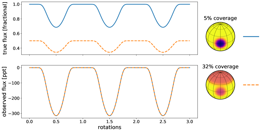
The top panel of Figure 11 shows two mock light curves we might compute following the procedure above. The solid blue curve corresponds to the light curve of a star with a single large equatorial spot of contrast $c$ viewed at an inclination $I=60^{\circ}$. The dashed orange curve corresponds to a star with a spot at the same location but half the contrast, plus a large polar spot of comparable contrast. Because the equatorial spot on this star has half the contrast of that on the first star, the peak-to-trough amplitude of the orange light curve is half that of the blue light curve. Moreover, since the polar spot is always in view on this star, the peak flux is itself only about half that of the first star. If we were given these two light curves in these fractional units, we might be able to infer these basic differences between the two stars (setting aside for the moment all the issues with the null space discussed in the previous section).

However, we do not observe stellar light curves in fractional units. Instead, we typically observe in units of counts on the detector, which depend (among other things) on various properties of the telescope. But even if we knew all these things, as well as the true luminosity of the star and the precise distance to it, and we could truly perform absolute photometry, that still would not be enough to correctly calibrate the light curve into the units we need. To convert to fractional units, we would need to know the brightness we would measure if the star had no spots on it. This depends on the brightness of the unspotted photosphere, which cannot be measured directly unless we actually resolve the star (i.e., interferometrically)!

Usually, this isn’t much of an issue. Astronomers typically circumvent this by self-normalizing the data: i.e., dividing the flux by the mean, median, maximum, or some similar statistic of the light curve. This operation folds the unknowability of the true units under the rug and transforms the light curve into a relative measurement of the star’s temporal variability. While relative measurements are typically what we are interested in anyways, this normalization procedure can sometimes fool us into thinking we have access to information that is simply not observable in single-band photometry. To understand why, consider the lower panel of Figure 11, which shows the same two light curves in what we will call relative units. To get the light curves in these units, we followed the common procedure of dividing each by the observed “continuum” level (the maximum flux in the light curve), subtracting unity, and multiplying by $1{,}000$, yielding relative fluxes in units of parts per thousand (ppt).

The two light curves, which were distinct in the fractional units we used to generate them, are indistinguishable in the relative units in which we observe them. There is absolutely no information in the relative light curves that can differentiate between the two stellar surfaces shown in the figure. The depth of each of the dips cannot tell us about either the contrast of individual spots or the total number of spots; in fact, in single-band photometry, these two quantities are perfectly degenerate with each other.

3.2 Ensemble analyses don’t necessarily help

To explore this point in a bit more detail, let us consider the normalization degeneracy in the context of ensemble analyses. Even though we can’t uniquely infer contrasts or numbers of spots from individual light curves, perhaps we could harness the power of the ensemble. Let us therefore go back to our thought experiment in which we added spots to a stellar surface. Assuming for simplicity that all spots have the same contrast $c$, every time we add a spot the flux (in fractional units) decreases by an amount proportional to $c$, so to first order we can approximate an individual light curve as

$$\mathbf{f}(c,n)=\mathbf{1}-c\sum_{i=0}^{n-1}\mathbf{g}(\boldsymbol{\theta}_{i})$$ (10)

where $\mathbf{g}(\boldsymbol{\theta}_{i})$ is some (complicated) function of the properties of the $i^{\mathrm{th}}$ spot as well as the stellar inclination, rotation period, etc., which we denote by $\boldsymbol{\theta}_{i}$. Now, consider many stellar light curves drawn from some distribution controlling the stellar and starspot properties with probability density $p(\boldsymbol{\theta})$. The mean of the distribution of light curves (still in fractional units) is then given by

$$\mu(c,n) =\mathrm{E}\Big{[}\mathbf{f}(c,n)\Big{]}$$

$$=1-c\,\mathrm{E}\bigg{[}\sum_{i=0}^{n-1}\mathbf{g}(\boldsymbol{\theta}_{i})\bigg{]}$$

$$=1-c\,n\,\alpha\hskip 0.0pt,$$ (11)

where $\mathrm{E}\big{[}\cdots\big{]}$ denotes the expected value and

$$\alpha\equiv\int\mathbf{g}(\boldsymbol{\theta})p(\boldsymbol{\theta})\mathrm{d}\boldsymbol{\theta}$$ (12)

is the expected value of $\mathbf{g}$. Similarly, the variance of the distribution may be computed as

$$\sigma^{2}(c,n) =\mathrm{Var}\Big{[}\mathbf{f}(c,n)\Big{]}$$

$$=\mathrm{Var}\Big{[}c\,\sum_{i=0}^{n-1}\mathbf{g}(\boldsymbol{\theta}_{i})\Big{]}$$

$$=c^{2}\,\mathrm{Var}\Big{[}\sum_{i=0}^{n-1}\mathbf{g}(\boldsymbol{\theta}_{i})\Big{]}$$

$$=c^{2}\sum_{i=0}^{n-1}\mathrm{Var}\Big{[}\mathbf{g}(\boldsymbol{\theta}_{i})\Big{]}$$

$$=c^{2}\,n\,(\beta^{2}-\alpha^{2})\hskip 0.0pt,$$ (13)

where $\mathrm{Var}\big{[}\cdots\big{]}$ denotes the variance,

$$\beta^{2}\equiv\int\mathbf{g}^{2}(\boldsymbol{\theta})p(\boldsymbol{\theta})\mathrm{d}\boldsymbol{\theta}$$ (14)

is the expected value of $\mathbf{g}^{2}$, and we used the fact that the variance of the sum of independent random variables is equal to the sum of their variances.

To summarize, the mean and variance of the ensemble of stellar light curves in fractional units is

$$\mu =1-c\,n\,\alpha$$

$$\sigma^{2} =c^{2}\,n\,(\beta^{2}-\alpha^{2})\hskip 0.0pt,$$ (15)

for some complicated functions $\alpha$ and $\beta$ of the distribution of stellar inclinations, rotation periods, and starspot properties. If our observations were collected in these fractional units, we could uniquely infer the spot contrast $c$ and the number of spots $n$, since these enter as $c\,n$ and $c^{2}n$ in the expressions for the mean and variance, respectively, and these are straightforward statistics to compute from the ensemble. However, because of observations are made in relative units, in which we typically normalize to the mean, the amplitudes of features in light curves can only tell us about the ratio

$$\frac{\sigma}{\mu} \propto\frac{c\sqrt{n}}{1-cn\alpha}$$ (16)

for some value of $\alpha$. In other words, even photometric ensemble analyses may not be able to tell us about the values of the contrast and the number of spots independently.

A direct consequence of this normalization degeneracy is that it may not be possible to uniquely constrain the total spot coverage of a star from single-band photometry without strong prior assumptions. The total spot coverage $f_{S}$ is simply the (average) area of a spot times the total number of spots divided by the total area of the sphere, which may be expressed as

$$f_{S}=\frac{1}{2}\left(1-\left<\cos r\right>\right)n\hskip 0.0pt,$$  (17)

given an angular spot radius $r$. While $r$ may be uniquely constrained from the covariance structure of the data (Paper II), $n$ cannot.

The arguments above are heuristic and based on only the first two moments of the distribution of light curves in an ensemble. It is possible, at least in principle, that higher order moments of the data could encode information to break the $c-n$ degeneracy, but these are in general more difficult to constrain from the data. It is also possible that we could place a lower limit on the spot contrast based on the normalized light curve. In Equation (10) we implicitly assumed that spots are allowed to overlap; under this assumption, it is possible to double the contrast of a spot by simply adding another spot on top of it. We could therefore generate light curves with arbitrarily large dips by choosing a small value for $c$ and a very large value for $n$. In reality, spots do not behave in this way: many overlapping spots likely still have the same effective temperature! Therefore, assuming there are no bright spots, the maximum depth of a feature in the light curve (even in relative units) could be used to place a lower limit on the spot contrast. Moreover, in Paper II we empirically show that, depending on the choice of prior, ensemble analyses may be able to place stronger constraints on the contrast $c$ than on the number of spots $n$.

Nevertheless, even with these caveats in mind, the fact remains that degeneracies like the polar spot effect are fundamental: recall Figure 11, in which the two stars have identical relative light curves, but very different spot coverage fractions. In general, any azimuthally-symmetric mode on the surface is in the null space of the normalized light curve problem. These components contribute a constant value to the flux at all phases, which effectively gets normalized away when we measure the light curve. A polar spot is just one manifestation of this degeneracy. Bands, or band-like arrangements of spots, will be at least partly in the null space of normalized light curves. These features change the total “spot coverage” of the surface but do not affect the light curve in a uniquely measurable way.

3.3 Effect on the covariance structure

There is one final subtle point concerning the normalization degeneracy that merits discussion. The common procedure of normalizing light curves to their mean, median, or maximum level does not only change the units of the data: it changes the very covariance structure of the light curves.

To understand why, let us consider the procedure of normalizing a light curve to its mean value. Whenever we scale our data, we must always be sure to scale the errorbars accordingly. Since in this case we are dividing the flux by the mean, one might imagine that we could simply divide each of the measurement uncertainties by the same amount. However, this is technically incorrect!

Figure 12: An example of why normalized light curves are non-stationary. The top panel shows $1{,}000$ samples from a unit-mean sinusoid with an amplitude of 10% and a period of 10 days, much longer than the 1 day observation baseline. The bottom panel shows the same light curves, each normalized to its own mean. Because the mean tends to be near the center of the observation window, points near $t=0.5$ are driven to values very close to unity, while points near the edges have much larger scatter.   

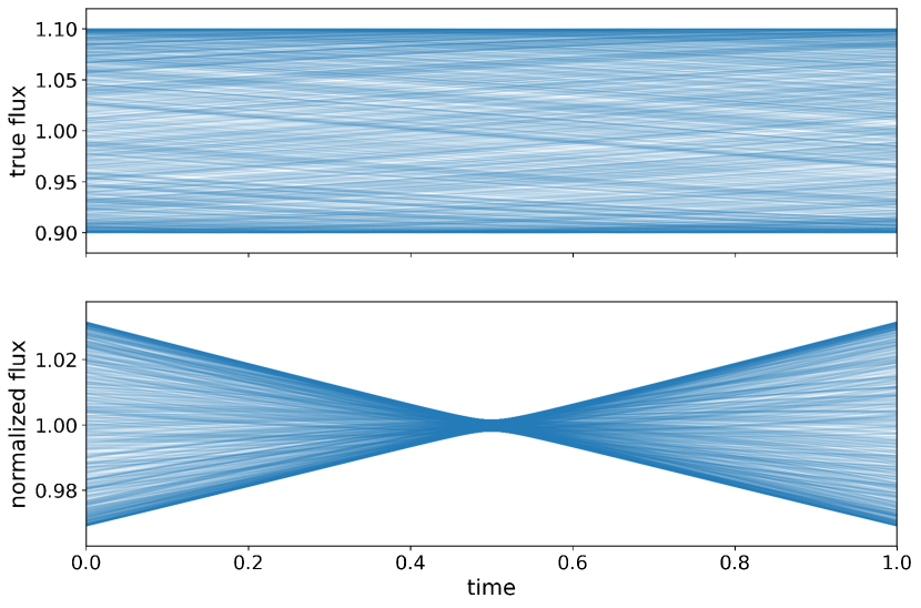
Consider the example in Figure 12. The top panel shows $1{,}000$ samples from a sinusoid with random phases and a period equal to ten times the observational window. In this limit, each light curve is approximately linear, which causes its mean value to roughly coincide with the midpoint of the observation window. Division by the mean value (lower panel) results in points near the midpoint being driven to unity and points near the edges (whose values differ the most from the mean) to be driven to both large and small values. If our error bars in the original data were uniform (homoscedastic), the error bars in the normalized light curves are not: the standard deviation (or variance) of the data is now distinctly dependent on the phase.

While the example shown in the figure is fairly extreme, the idea here is quite general: the normalization procedure changes the covariance structure of the data. In most cases, the non-stationarity (i.e., the phase dependence) of the variance will be quite small. The effect is primarily important for light curves with periods much longer than the observation window. In these cases, not accounting for this effect could introduce bias in light curve analyses. A detailed investigation of this effect is beyond the scope of this paper, but we do present a method to correct the covariance matrix of normalized light curves for this issue in Paper II.

4 Discussion and conclusions

4.1 Degeneracies stemming from the null space

In this paper we explored various degeneracies in the problem of inferring a stellar surface map from its rotational light curve. We discussed the idea behind the null space, the set of surface modes that have exactly zero effect on the observed light curve (§2). For rotational light curves, we showed that the vast majority of the information about the surface intensity is in the null space and therefore cannot be inferred from unresolved photometric measurements. We showed, in particular, that the size of the null space grows quadratically with increasing spatial resolution, while the number of independent degrees of freedom in the light curve only grow linearly. Consequently, the information content of light curves is small for large scale surface features and vanishingly small for small scale features.

A direct consequence of this fact is that results based on analyses of individual light curves are often extremely sensitive to the particular assumptions of one’s model. We therefore urge lots of care in these kinds of analyses, where assumptions of uniform-contrast, discrete, and circular spots, or alternatively of maximum entropy or “simplicity” may result in significant bias. In this respect, we agree with the recent paper by Basri & Shah (2020), which cautions against the association of invidual dips in light curves with individual, discrete spots.

One of the main results in this paper concerning the null space is its dependence on stellar inclination (§2.4). Because the modes that lie in the null space change depending on the viewing angle, observations of a star at many inclinations would break many of the degeneracies in the mapping problem. While this is obviously infeasible in practice, the dependence of the null space on inclination motivates ensemble analyses of many similar stars as a way of circumventing the mapping degeneracies by providing a strong data-driven prior. As we show in Paper II in this series, the joint analysis of tens to hundreds of light curves can uniquely constrain the distribution of starspot sizes and latitudes among the stars in the sample. In that paper, we show that ensemble analyses can even break the latitude-inclination degeneracy (e.g., Walkowicz et al., 2013), allowing one to infer individual stellar inclinations, typically to within about $10^{\circ}$.

We also showed how the null space is a strong function of the stellar limb darkening. While this can again be used to our advantage—by harnessing the variance in the limb darkening parameters across an ensemble of stellar light curves—in practice it is likely to complicate inference, since any bias in the assumed limb darkening coefficients will likely result in bias in the inferred surface properties. We revisit this point in Paper II.

One final point that we did not address thus far concerns occultations. Our results regarding the null space apply strictly to rotational light curves, in which all points on the projected disk contribute to the measured flux. During an occultation by a transiting planet or a binary companion, the weighting of surface modes giving rise to the light curve changes substantially. In fact, the presence of an occultor breaks many of the perfect symmetries that give rise to a null space in the first place (e.g., Luger et al., 2019). This fact can be used to infer the properties of spots in the path of the occultor, as was done (for example) by Morris et al. (e.g., 2017). A detailed investigation of the null space for the occultation problem is beyond the scope of this work.

4.2 Degeneracies due to the unknown normalization

The second major source of degeneracies is the fundamental unknowability of the true normalization in single-band photometry (§3), which is summarized in Figure 11. In a nutshell, the relationship between the amplitude of a feature in the light curve and the contrast of the feature that gave rise to it depends on quantities like the unspotted photospheric brightness, which is not an observable in single-band photometry. This leads to the possibility of distinctly different stellar surfaces having identical relative light curves, as demonstrated in the figure.

In practice, this degeneracy usually manifests as a nonlinear correlation between the contrast $c$ of a spot and the total number $n$ of spots on the surface of the star. Even in ensemble analyses, one cannot in general learn these two quantities independently from the data alone, only a (complicated) function of the two (Equation 16). In Paper II we show empirically that careful analysis of the covariance structure of ensembles of light curves may shed some light on $c$ but cannot uniquely constrain $n$. A direct consequence of this degeneracy is that constraints on the total number of spots or on the spot coverage of a star from single-band light curves depend strongly on the model assumptions.

Recently, Morris (2020b) performed an ensemble analysis of Kepler, K2, and TESS light curves to derive a relationship between the fractional spot coverage $f_{S}$ and stellar age. That work found that the spot coverage $f_{S}$ as a function of age is well modeled by a simple power law, decreasing from ${\sim}10\%$ for the youngest (${\sim}10$ Myr) stars to less than $1\%$ for the oldest (${\sim}5$ Gyr) stars. While this broadly agrees with the expectation that stellar magnetic activity decreases over time, our work strongly suggests that these results depend heavily on the prior. This is because the expression for $f_{S}$ (Equation 17) depends on two quantities: the average spot radius $r$, which can be constrained (see Luger et al., 2021), and the total number of spots $n$, which we showed cannot be uniquely constrained from single-band light curves. In fact, Morris (2020b) assumed $n=3$ for simplicity when doing posterior inference. We therefore urge care in interpreting those results, as it is possible this assumption does not hold across the large range of spectral types and stellar ages considered in that study. Nevertheless, the other central result of that paper, the relationship between the “smoothed amplitude” of a light curve and the stellar age, is valid. Moreover, the core idea in Morris (2020b) (and in related studies such as Jackson & Jeffries, 2013) is very similar to that advocated here: the use of ensemble analyses to constrain population-level parameters when invidual datasets are not sufficiently constraining.

Another recent paper relevant to our work is that of Basri & Shah (2020), who investigated the information content of stellar light curves, exploring what can and cannot be learned about star spot configurations from individual light curves. That paper strongly urges against the common practice of interpreting light curves with one or two dips as originating from one or two spots, respectively, a point we strongly agree with (see our Figure 1). It also reinforces our point about the additional degeneracies introduced by the unknown normalization inherent to single-band photometry.

As with the degeneracies due to the null space, there are potential ways to break the normalization degeneracy. In principle, the maximum level of a light curve could set a lower limit on the brightness of the unspotted photosphere, particularly for long-baseline, time-variable surfaces (Basri, 2018). However, this would work only if the surface is known to be made up exclusively of dark spots. The presence of bright spots (faculae), which are common on the Sun, make it difficult for one to infer this quantity (and hence the correct normalization) from single-band photometry in practice.

A better approach may be to collect photometric data in multiple wavelength bands, an idea that has been explored recently (e.g., Gully-Santiago et al., 2017; Guo et al., 2018). Assuming the locations and sizes of a star’s spots are constant in wavelength, the amplitude of the light curve in different bands (and in particular its slope as a function of wavelength) can be used to directly constrain the temperature, and hence the contrast, of the spots. This effectively breaks the $c-n$ degeneracy. In practice, the effective size of spots may be different at different wavelengths, which could complicate this picture somewhat, but the point still stands that light curves collected in multiple bands contain at least partial information about the correct normalization. A more detailed analysis of the information content of multi-band light curves, and, by extension, spectroscopic timeseries, is deferred to a future paper in this series.

4.3 Caveats

There are several simplifying assumptions we made in this paper that are worth discussing. First, in our characterization of the null space we assumed we knew the stellar inclination, the stellar rotation period, and the limb darkening coefficients exactly, and we computed the information content of stellar light curves in the limit of infinite SNR. None of these assumptions are valid in practice. In realistic scenarios, the variance reduction will be necessarily lower than what we presented here: the curves in Figure 7, for instance, are therefore strict upper bounds on the amount of information that can be learned about the surface. In some cases, it may be possible to infer the inclination from spectroscopic $v\sin I$ measurements, or the limb darkening coefficients from the shape of transiting exoplanet light curves; but any uncertainty in these quantities will degrade our ability to constrain information about the surface.

Moreover, our constraints on the information content of ensembles of light curves are also strict upper limits, since we assumed all stars in the ensemble are identical. Variance in the surface maps of stars in a population makes it effectively impossible to infer detailed properties of the individual stellar surfaces in the ensemble. We argued without proof that what we can learn instead are properties of the distribution of stellar surfaces among the population, such as the distribution of spot sizes and active latitudes. Demonstrating this point is more difficult, so we defer it to Paper II, where we construct a custom Gaussian process model and show that it can be used to infer such population-level parameters from ensembles of light curves.

Finally, we limited our discussion to static stellar surfaces. Real stellar surfaces vary with time as individual spots form, evolve, and dissipate, or as a star progresses through its activity cycle. This, too, makes it more difficult to constrain the stellar surface at a particular point in time, since the amount of data corresponding to a particular surface configuration is more limited. On the other hand, a time-variable surface could be used to our advantage from an ensemble standpoint. Although we are unable to uniquely infer invididual spot properties, we could treat each point in the light curve as a realization of a random process (i.e., a draw from some distribution) describing the stellar surface at a high level. In this sense, we could harness the fact that we can measure the light curves of many “similar” surfaces to learn something about their statistical properties. Demonstrating this is beyond the scope of the present work, but we return to this point in Paper II.

4.4 Future work

This paper is the first in a series dedicated to developing methodology to infer stellar surface properties from unresolved measurements. It sets the stage for Luger et al. (2021), in which we develop an interpretable Gaussian process (GP) model for starspot-induced light curve variability. This GP is aimed specifically at the difficult problem of jointly modeling many light curves in an ensemble analysis. Although we hinted at this here, we will show in that paper that ensemble analyses can uniquely constrain several statistical properties of starspots, including their distribution of radii and latitudes across stars in the ensemble. In that work we also consider temporally evolving surfaces, which we neglected in our discussion thus far.

Finally, while this paper explicitly dealt with the problem of photometric rotational light curves, the degeneracies outlined here and the methodology developed in this series of papers apply more broadly in other contexts. These including applications where the stellar surface is a nuisance (exoplanet detection and characterization using transit light curves or radial velocities) and spectral time series datasets (such as transmission spectroscopy and Doppler imaging).

In keeping with other papers in the starry series, all figures in this paper are generated automatically from open-source scripts linked to in each of the captions , and the principal equations link to associated unit tests that ensure the accuracy and reproducibility of the algorithm presented here /.

We would like to thank Michael Gully-Santiago, Fran Bartolić, and the Astronomical Data Group at the Center for Computational Astrophysics for many thought-provoking discussions that helped shape this paper.

Appendix A Decomposition of the flux operator

In this section we show how to use singular value decomposition (SVD) to decompose a surface map into its preimage and its null space (see §2.2). By performing SVD, we may express the flux design matrix as

$$\boldsymbol{\mathcal{A}}=\mathbf{U}\,\mathbf{S}\,\mathbf{V}^{\top}\hskip 0.0pt,$$ (A1)

where $\mathbf{U}$ is a $(K\times K)$ orthogonal matrix, $\mathbf{V}$ is a $(N\times N)$ orthogonal matrix, and $\mathbf{S}$ is a $(K\times N)$ diagonal matrix. The columns of $\mathbf{U}$ and the rows of $\mathbf{V}^{\top}$ are the left and right singular vectors of $\boldsymbol{\mathcal{A}}$, and the entries along the diagonal of $\mathbf{S}$ are the corresponding singular values, arranged in descending order. If $\boldsymbol{\mathcal{A}}$ has rank $R$, the first $R$ singular values will be nonzero, while the remaining $N-R$ will be identically zero. If we assume for definitess that $K>N$ (i.e., we have more flux observations than surface map coefficients we’re trying to constrain), we can express the matrices in Equation (A1) as

$$\mathbf{U} =\left(\begin{array}[]{ccc|ccc}\mathbf{U}_{0,0}&\cdots&\mathbf{U}_{0,R\text{-}1}&\mathbf{U}_{0,R}&\cdots&\mathbf{U}_{0,K\text{-}1}\\ \vdots&\cdots&\vdots&\vdots&\cdots&\vdots\\ \mathbf{U}_{K\text{-}1,0}&\cdots&\mathbf{U}_{K\text{-}1,R\text{-}1}&\mathbf{U}_{K\text{-}1,R}&\cdots&\mathbf{U}_{K\text{-}1,K\text{-}1}\end{array}\right)\equiv\left(\begin{array}[]{c|c}\mathbf{U}_{\bullet}&\mathbf{U}_{\circ}\end{array}\right)$$ (A6)

$$\mathbf{S} =\left(\begin{array}[]{ccc|ccc}\mathbf{S}_{0,0}\phantom{y}&&&&&\\ &\ddots&&&\mbox{\Large 0}&\\ &&\mathbf{S}_{R\text{-}1,R\text{-}1}&&&\\ \hline\cr&&&\mathbf{S}_{R,R}\phantom{y}&&\\ &\mbox{\Large 0}&&&\ddots&\\ &&&&&\mathbf{S}_{N\text{-}1,N\text{-}1}\\ &&&&&\\ &\mbox{\Large 0}&&&\mbox{\Large 0}&\\ &&&&&\end{array}\right)\equiv\left(\begin{array}[]{c|c}\mathbf{S}_{\bullet}&\mathbf{0}\\ \hline\cr\mathbf{0}&\mathbf{S}_{\circ}\end{array}\right)$$ (A18)

$$\mathbf{V}^{\top} =\left(\begin{array}[]{cccccc}\mathbf{V}_{0,0}^{\top}&\cdots&\mathbf{V}_{0,N\text{-}1}^{\top}\\ \vdots&\cdots&\vdots\\ \mathbf{V}_{R\text{-}1,0}^{\top}&\cdots&\mathbf{V}_{R\text{-}1,N\text{-}1}^{\top}\\[5.0pt] \hline\cr\\[-8.50006pt] \mathbf{V}_{R,0}^{\top}&\cdots&\mathbf{V}_{R,N\text{-}1}^{\top}\\ \vdots&\cdots&\vdots\\ \mathbf{V}_{N\text{-}1,0}^{\top}&\cdots&\mathbf{V}_{N\text{-}1,N\text{-}1}^{\top}\end{array}\right)\equiv\left(\begin{array}[]{cc}\mathbf{V}_{\bullet}^{\top}\\ \hline\cr\mathbf{V}_{\circ}^{\top}\end{array}\right)$$ (A28)

where $\mathbf{U}_{\bullet}$ is $(K\times R)$, $\mathbf{U}_{\circ}$ is $(K\times K-R)$, $\mathbf{S}_{\bullet}$ is $(R\times R)$, $\mathbf{S}_{\circ}$ is $(K-R\times N-R)$, $\mathbf{V}_{\bullet}^{\top}$ is $(R\times N)$, and $\mathbf{V}_{\circ}^{\top}$ is $(N-R\times N)$. We may then express the decomposition of $\boldsymbol{\mathcal{A}}$ as

$$\boldsymbol{\mathcal{A}}=\left(\begin{array}[]{c|c}\mathbf{U}_{\bullet}&\mathbf{U}_{\circ}\end{array}\right)\left(\begin{array}[]{c|c}\mathbf{S}_{\bullet}&\mathbf{0}\\ \hline\cr\mathbf{0}&\mathbf{S}_{\circ}\end{array}\right)\left(\begin{array}[]{cc}\mathbf{V}_{\bullet}^{\top}\\ \hline\cr\mathbf{V}_{\circ}^{\top}\end{array}\right)\hskip 0.0pt.$$ (A34)

Inserting this into Equation (1), we have

$$\mathbf{f}-\mathbf{1} =\boldsymbol{\mathcal{A}}\,\mathbf{y}$$

$$=\left(\begin{array}[]{c|c}\mathbf{U}_{\bullet}&\mathbf{U}_{\circ}\end{array}\right)\left(\begin{array}[]{c|c}\mathbf{S}_{\bullet}&\mathbf{0}\\ \hline\cr\mathbf{0}&\mathbf{S}_{\circ}\end{array}\right)\left(\begin{array}[]{cc}\mathbf{V}_{\bullet}^{\top}\\ \hline\cr\mathbf{V}_{\circ}^{\top}\end{array}\right)\mathbf{y}$$  (A40)

$$=\mathbf{U}_{\bullet}\,\mathbf{S}_{\bullet}\,\mathbf{V}_{\bullet}^{\top}\,\mathbf{y}+\mathbf{U}_{\circ}\,\mathbf{S}_{\circ}\,\mathbf{V}_{\circ}^{\top}\,\mathbf{y}$$

$$=\mathbf{U}_{\bullet}\,\mathbf{S}_{\bullet}(\,\mathbf{I}\,)\mathbf{V}_{\bullet}^{\top}\,\mathbf{y}+\mathbf{U}_{\circ}\,\mathbf{S}_{\circ}(\,\mathbf{I}\,)\mathbf{V}_{\circ}^{\top}\,\mathbf{y}$$

$$=\mathbf{U}_{\bullet}\,\mathbf{S}_{\bullet}(\mathbf{V}_{\bullet}^{\top}\mathbf{V}_{\bullet})\mathbf{V}_{\bullet}^{\top}\,\mathbf{y}+\mathbf{U}_{\circ}\,\mathbf{S}_{\circ}(\mathbf{V}_{\circ}^{\top}\mathbf{V}_{\circ})\mathbf{V}_{\circ}^{\top}\,\mathbf{y}$$

$$=(\mathbf{U}_{\bullet}\,\mathbf{S}_{\bullet}\,\mathbf{V}_{\bullet}^{\top})\mathbf{V}_{\bullet}\mathbf{V}_{\bullet}^{\top}\,\mathbf{y}+(\mathbf{U}_{\circ}\,\mathbf{S}_{\circ}\,\mathbf{V}_{\circ}^{\top})\mathbf{V}_{\circ}\mathbf{V}_{\circ}^{\top}\,\mathbf{y}$$

$$=(\mathbf{U}_{\bullet}\,\mathbf{S}_{\bullet}\,\mathbf{V}_{\bullet}^{\top})\,\mathbf{y}_{\bullet}+(\mathbf{U}_{\circ}\,\mathbf{S}_{\circ}\,\mathbf{V}_{\circ}^{\top})\,\mathbf{y}_{\circ}$$  (A41)

where we define

$$\mathbf{y}_{\bullet} \equiv\mathbf{P}\,\mathbf{y}$$  (A42)

$$\mathbf{y}_{\circ} \equiv\mathbf{N}\,\mathbf{y}$$  (A43)

$$\mathbf{P} \equiv\mathbf{V}_{\bullet}\mathbf{V}_{\bullet}^{\top}$$  (A44)

$$\mathbf{N} \equiv\mathbf{V}_{\circ}\mathbf{V}_{\circ}^{\top}\hskip 0.0pt,$$  (A45)

and we used the fact that since $\mathbf{V}^{\top}$ is orthogonal,

$$\mathbf{V}_{\bullet}^{\top}\mathbf{V}_{\bullet} =\mathbf{I}$$

$$\mathbf{V}_{\circ}^{\top}\mathbf{V}_{\circ} =\mathbf{I}\hskip 0.0pt,$$  (A46)

where $\mathbf{I}$ is the identity matrix. Now, recalling that $R$ is the number of nonzero singular values in $\mathbf{S}$, it is evident from Equation (A18) that

$$\mathbf{S}_{\circ}=\mathbf{0}\hskip 0.0pt.$$ (A47)

Therefore we may write Equation (A) as

$$\boxed{\mathbf{f}=\mathbf{1}+\boldsymbol{\mathcal{A}}\,\mathbf{y}_{\bullet}+\mathbf{0}\,\mathbf{y}_{\circ}}$$  (A48)

where the fact that $\mathbf{U}_{\bullet}\,\mathbf{S}_{\bullet}\,\mathbf{V}_{\bullet}^{\top}=\boldsymbol{\mathcal{A}}$ follows directly from Equations (A34) and (A47). This is the decomposition of the surface map $\mathbf{y}$ into its preimage $\mathbf{y}_{\bullet}$ and null space $\mathbf{y}_{\circ}$ components.

Two things should be noted concerning this derivation. First, because of the orthogonality of $\mathbf{V}$,

$$\mathbf{V}\mathbf{V}^{\top} =\mathbf{I}$$

$$\mathbf{V}_{\bullet}\mathbf{V}_{\bullet}^{\top}+\mathbf{V}_{\circ}\mathbf{V}_{\circ}^{\top} =\mathbf{I}$$

$$\mathbf{P}+\mathbf{N} =\mathbf{I}\hskip 0.0pt,$$  (A49)

so it follows from Equations (A42) and (A43) that $\mathbf{y}=\mathbf{y}_{\bullet}+\mathbf{y}_{\circ}$.

Second, the singular value decomposition is not always unique. The matrix of singular values $\mathbf{S}$ is unique provided we arrange them in decreasing order, but if there are degenerate or zero-valued singular values (as is the case here), the matrices $\mathbf{U}$ and $\mathbf{V}^{\top}$ (and thus $\mathbf{V}^{\top}_{\bullet}$ and $\mathbf{V}^{\top}_{\circ}$) are only well-defined up to arbitrary unitary transformations. However, the quantities $\mathbf{V}_{\bullet}\mathbf{V}^{\top}_{\bullet}$ and $\mathbf{V}_{\circ}\mathbf{V}^{\top}_{\circ}$ (which define the operators $\mathbf{P}$ and $\mathbf{N}$ above) are unique, so the decomposition into null space and preimage is always well-defined.

References

- Agol et al. (2020) Agol, E., et al. 2020, AJ, 159, 123
- Basri (2018) Basri, G. 2018, ApJ, 865, 142
- Basri & Shah (2020) Basri, G., & Shah, R. 2020, ApJ, 901, 14
- Berdyugina (2005) Berdyugina, S. V. 2005, Living Reviews in Solar Physics, 2, 8
- Betancourt (2018) Betancourt, M. 2018, arXiv e-prints, arXiv:1803.08393
- Borucki et al. (2010) Borucki, W. J., et al. 2010, Science, 327, 977
- Cowan et al. (2013) Cowan, N. B., et al. 2013, MNRAS, 434, 2465
- Cowan et al. (2009) —. 2009, ApJ, 700, 915
- Davenport et al. (2015) Davenport, J. R. A., et al. 2015, ApJ, 806, 212
- Fienup (1982) Fienup, J. 1982, Applied optics, 21, 2758
- Garraffo et al. (2018) Garraffo, C., et al. 2018, ApJ, 862, 90
- Gully-Santiago et al. (2017) Gully-Santiago, M. A., et al. 2017, ApJ, 836, 200
- Guo et al. (2018) Guo, Z., et al. 2018, ApJ, 868, 143
- Harmon & Crews (2000) Harmon, R. O., & Crews, L. J. 2000, AJ, 120, 3274
- Hogg & Villar (2021) Hogg, D. W., & Villar, S. 2021, arXiv e-prints, arXiv:2101.07256
- Jackson & Jeffries (2013) Jackson, R. J., & Jeffries, R. D. 2013, MNRAS, 431, 1883
- Kopal (1950) Kopal, Z. 1950, Harvard College Observatory Circular, 454, 1
- Lanza et al. (2011) Lanza, A. F., et al. 2011, A&A, 533, A44
- Luger et al. (2019) Luger, R., et al. 2019, AJ, 157, 64
- Luger et al. (2021) —. 2021, arXiv e-prints, arXiv:2102.01697
- Morris (2020a) Morris, B. 2020a, The Journal of Open Source Software, 5, 2103
- Morris (2020b) Morris, B. M. 2020b, ApJ, 893, 67
- Morris et al. (2017) Morris, B. M., et al. 2017, ApJ, 846, 99
- Rackham et al. (2018) Rackham, B. V., et al. 2018, ApJ, 853, 122
- Rauscher et al. (2018) Rauscher, E., et al. 2018, AJ, 156, 235
- Ricker et al. (2015) Ricker, G. R., et al. 2015, Journal of Astronomical Telescopes, Instruments, and Systems, 1, 014003
- Roettenbacher et al. (2017) Roettenbacher, R. M., et al. 2017, ApJ, 849, 120
- Russell (1906) Russell, H. N. 1906, ApJ, 24, 1
- Sandford & Kipping (2019) Sandford, E., & Kipping, D. 2019, AJ, 157, 42
- Vogt et al. (1987) Vogt, S. S., et al. 1987, ApJ, 321, 496
- Walkowicz et al. (2013) Walkowicz, L. M., et al. 2013, ApJS, 205, 17