Input-output behaviour of a model neuron
with alternating drift

Abstract

The input-output behaviour of the Wiener neuronal model subject to alternating input is studied under the assumption that the effect of such an input is to make the drift itself of an alternating type. Firing densities and related statistics are obtained via simulations of the sample-paths of the process in the following three cases: the drift changes occur during random periods characterized by (i) exponential distribution, (ii) Erlang distribution with a preassigned shape parameter, and (iii) deterministic distribution. The obtained results are compared with those holding for the Wiener neuronal model subject to sinusoidal input.

Keywords: Wiener neuronal model; firing densities; alternating drift.

1 Introduction

During the last four decades numerous efforts have been devoted to the construction of mathematical models aiming at the description of single neuron’s firing processes. A customary feature of widespread existing models is the assumption that the neurons’ firing is described by the first passage of the membrane potential through a threshold, the membrane potential being viewed as a continuous stochastic process. Great attention has being put on the identification of suitable Markov processes and firing thresholds, especially with a view to include in the model certain relevant features, such as the effects of external input on the neuron’s response (see Ricciardi, 1995, and Ricciardi et al., 1999, for a description of neuronal models and methods to face the first-passage-time problem).

Within such a background, in this paper we study the input-output behaviour of model neurons subject to alternating input, assuming that excitatory stimuli prevail on inhibititory stimuli, and viceversa, during randomly alternating time intervals. The membrane potential is assumed to be described by a Wiener process; the effects of the alternating stimuli is condensed in the drift. The first passage through constant firing thresholds is analyzed by constructing estimated firing densities. This is obtained by making use of an ad hoc procedure for the simulation of sample paths of the Wiener process with alternating drift. The effect of alternating stimuli on the firing densities is analyzed when the drift changes occur during random periods characterized by (i) exponential distribution, (ii) Erlang distribution with shape parameter 2, and (iii) deterministic distribution. The computational results obtained for the considered model are then compared with those holding for the Wiener neuronal model subject to sinusoidal input.

Let us now point out some specific features of this paper with a view to relate them to other works in the field. First of all, as mentioned in Lánský et al. (2001), the interpretation of the neuronal firing times in terms of alternating periods appears to be natural for some types of neurons. It should be also mentioned that a similar problem was analyzed in Bulsara et al. (1994), where the first passage time problem of a Wiener process with sinusoidal time-varying drift through a constant threshold is treated. Our proposed model, however, offers the advantages that the epochs of high and low stimulation can be of different lengths; moreover, due to its greater flexibility, it allows to describe time-varying inputs characterized by more general shapes than sinusoidal ones.

2 The Wiener model

As customary, we assume that the neuron’s membrane potential is described by a continuous one-dimensional stochastic process $\{X(t);\,t\geq 0\}$ representing the changes in the membrane potential between two consecutive neuronal firings, the firing threshold being a constant $\beta$. Assuming that $X(0)=x_{0}<\beta$, the FPT random variable

$$T=\inf\{t\geq 0\colon\,X(t)>\beta\}$$

describes the neuronal interspike intervals. An essential problem is to determine the p.d.f. of $T$, i.e. the firing density

$$g(\beta,t\,|\,x_{0})={\partial\over\partial t}\,\Pr(T\leq t),\quad t>0.$$

A first well-known neuronal model was proposed by Gerstein and Mandelbrot (1964), who assumed that the neuron’s membrane potential undergoes a simple random walk under the effect of excitatory and inhibitory synaptic actions. This assumption, upon a suitable limit procedure, leads to the Wiener process

$$X(t)=x_{0}+\xi\,t+\sigma\,B(t),\quad t>0,$$

with $x_{0}\in{\bf R}$, $\xi\in{\bf R}$ and $\sigma>0$, and where $B(t)$ denotes the standard Brownian motion. Even though the assumptions of this model are oversimplified as they do not take into account certain properties such as the spontaneous exponential decay of the membrane potential in the absence of input, the Wiener model can be usefully treated as a starting point for investigations on neuronal stochastic models. For instance, the Wiener model with random jumps has been considered recently by Giraudo et al. (2001) as a model for the description of changes in the membrane potential depending on the distance between the trigger zone and the synaptic ending.

3 Wiener model with alternating drift

Our present aim is to analyse the input-output behaviour of the Wiener model subject to alternating input. To such a purpose, we assume that the effects of alternating stimuli reflect into the drift of the Wiener process. This leads to a Wiener process with alternating drift, described by

$$X(t)=x_{0}+\int_{0}^{t}\xi(s)\,{\rm d}s+\sigma\,B(t),\quad t\geq 0,$$ (1)

where $x_{0}\in{\bf R}$, $\sigma>0$ and $\{\xi(t);\,t\geq 0\}$ is a dichotomous stochastic process on states $c$ and $-v$, with $c,v>0$ and $\xi(0)=c$. Eq. (1) describes a Brownian motion that starts from $x_{0}$ at time $0$, with positive drift $c$ and infinitesimal variance $\sigma^{2}$. Denoting by $Y_{1},Y_{2},\ldots$ the independent random times separating consecutive changes of the drift value, we have $\xi(t)=c$ during the random periods of lengths $Y_{1},Y_{3},Y_{5},\ldots$ and $\xi(t)=-v$ during the remaining random periods. Formally,

$$\xi(t)=\frac{c-v}{2}+\frac{c+v}{2}\,(-1)^{N(t)},\quad t\geq 0,$$

where

$$N(t)=\sum_{k=1}^{\infty}{\bf 1}_{\{Y_{1}+\cdots+Y_{k}\leq t\}},\quad t\geq 0.$$

At the random times $Y_{1}+\cdots+Y_{k}$ the value of $\xi(t)$ thus changes from $c$ to $-v$ if $k$ is odd, and from $-v$ to $c$ if $k$ is even. We also assume that the non-negative random variables $Y_{1},Y_{3},Y_{5},\ldots$ and $Y_{2},Y_{4},Y_{6},\ldots$ have distribution functions $F_{U}(t)$ and $F_{D}(t)$, respectively, so that the random periods during which the drift is positive (resp. negative) are i.i.d. We remark that the probability law of (1) can be expressed as a mixture of Gaussian densities (see Di Crescenzo, 2000).

4 Estimating the firing density via simulations

In this Section we shall determine the firing density of the Wiener neuronal model with alternating drift in the presence of a constant firing threshold $\beta$. Making use of a direct analysis of the sample-paths of process (1), it is possible to obtain a series expression of the firing density. Unfortunately, the series involves integrals of progressively increasing dimensionality, so that such an analytic result is unsuitable for practical purposes. Nevertheless, by truncation to the first few terms the following lower bound for the firing density is obtained: For all $t>0$ and $\beta>x_{0}$ we have

$$g(\beta,t\,|\,x_{0})\geq[1-F_{U}(t)]\,\widetilde{g}_{c}(\beta,t\,|\,x_{0})+\int_{0}^{t}\int_{-\infty}^{\beta}[1-F_{D}(t-u)]\,\widetilde{g}_{-v}(\beta,t-u\,|\,x)\alpha(x,u\,|\,x_{0})\,{\rm d}x\,{\rm d}F_{U}(u),$$

where $\widetilde{g}_{\eta}(\beta,t\,|\,x_{0})$ is the first-passage-time density of a Wiener process with drift $\eta$ throught $\beta$,

$$\widetilde{g}_{\eta}(\beta,t\,|\,x_{0})={\beta-x_{0}\over\sqrt{2\pi\sigma^{2}t^{3}}}\exp\left\{-{(\beta-x_{0}-\eta t)^{2}\over 2\sigma^{2}t}\right\},$$

while $\alpha(x,t\,|\,x_{0})$ is the $\beta$-avoiding density of a Wiener process with drift $c$,

$$\alpha(x,t\,|\,x_{0})={1\over\sqrt{2\pi\sigma^{2}t}}\exp\left\{-{(x-x_{0}-c\,t)^{2}\over 2\sigma^{2}t}\right\}\left[1-\exp\left\{-{2\over\sigma^{2}t}\,(\beta-x)\,(\beta-x_{0})\right\}\right].$$

In order to obtain histograms as estimates of the firing densities, we resort to simulations of the sample paths of process (1). This is performed by making use of a procedure that is strictly based on the properties of the underlying Wiener process. Such procedure simulates the sample-paths of process (1) at the random times where the drift alternates.

A sketch of the procedure for the simulation of $T$ is given below:

Begin Procedure
0.  $x:=x_{0}$, $t:=0$, $\xi:=c$;
1.  generate an inversion instant $\tau$;
2.  $p:=\Pr\{$the first passage occurs before $\tau\}$;
3.  generate an uniform pseudo-random number $u$ in $(0,1)$;
4.  if $u>p$ then goto Step 7;
5.  generate a pseudo-random number $\theta$ in $(0,\tau)$ from p.d.f. $f_{1}(\theta)$;
6.  $fpt:=\theta+t$; output($fpt$); stop;
7.  generate a pseudo-random number $z$ in $(-\infty,\beta)$ from p.d.f. $f_{2}(z)$;
8.  $x:=z$, $t:=t+\tau$; update $\xi$;
9.  goto Step 1;
End Procedure

For Step 1 we assume that the random inversion times having distributions $F_{U}$ and $F_{D}$ can be numerically simulated.

Let us informally discuss the underlying ideas of this procedure. After the first drift inversion time $\tau$ has been generated, a Bernoulli trial with success probability $p$ is simulated (Step 2), where $p$ is the FPT probability

$$p:=P(T\leq\tau)=\Phi\left(-\displaystyle{\beta-x-\xi\tau\over\sigma\sqrt{\tau}}\right)+e^{2\xi(\beta-x)/\sigma^{2}}\,\Phi\left(-\displaystyle{\beta-x+\xi\tau\over\sigma\sqrt{\tau}}\right),$$

$\Phi$ denoting the standard normal distribution function. A success of the Bernoulli trial means that the first passage has occurred before time $\tau$. In such a case the FPT is simulated via $f_{1}$, which is the FPT density of a Wiener process through $\beta$ conditional on $\{T\leq\tau\}$, and the simulation ends. If a failure occurs in the Bernoulli trial, then the value attained by the Wiener process at time $\tau$ is simulated via density $f_{2}$, which is the density of $X(\tau)$ conditional on $\{T>\tau\}$. Densities $f_{1}$ and $f_{2}$, whose analytic expressions are known, are simulated by making use of a standard Von Neumann acceptance-rejection method (see for instance Rubinstein, 1981). After $X(\tau)$ has been generated, the current drift $\eta$ is updated to the new value, i.e. $-v$ if it was $c$, and vice-versa. The simulation than proceeds, restarting afresh by generating a new inversion time of the drift, and so on until the first passage through $\beta$ occurs.

We point out that, according to the assumptions of our model, the case of endogenous periodicity is developed in the given procedure. In other words, the input is reset after that the threshold is reached. However, we point out that the case of exhogenous periodicity could be considered upon an easy modification of the procedure (useful references on the effects of endogenous and exhogenous periodicity are the papers by Lánský (1997) and Plesser and Geisel (2001)).

In the following sections we discuss the results obtained in three special cases for the drift inversion times: (i) exponentially distributed times, (ii) Erlang distributed times, and (iii) deterministic times. The shown estimates of the firing density $g(\beta,t\,|\,x_{0})$ are obtained via simulation of $10^{6}$ sample-paths of $X(t)$.

5 Exponentially distributed inversion times

Let us assume that the inversion times of the Wiener neuronal model (1) have distribution functions $F_{U}(t)=1-e^{-\lambda t}$ and $F_{D}(t)=1-e^{-\mu t}$, $t\geq 0$. Thus, $\lambda^{-1}$ is the mean of the random periods during which the excitatory stimuli prevail on inhibitory stimuli, while $\mu^{-1}$ is the mean of the random periods with opposite behaviour. We have considered some cases of interest in the physiological contexts, with $\mu\geq\lambda$, with threshold $\beta=10$, and with $x_{0}=0$.

The most evident feature of the estimated firing densities is their being unimodal (see Figure 1). In particular, if $\mu$ increases the mode $m$ increases while the median $q_{2}$ decreases, as well as the quartiles $q_{1}$ and $q_{3}$, and the inter-quartile range $IQR$. This is in agreement with the fact that if $\mu$ increases, the random periods with prevailing inhibitory stimuli becomes ‘smaller’ in stochastic sense. A quite similar behaviour is observed if $\lambda$ decreases (see Figure 2). Moreover, as $\sigma$ increases the firing density becomes less peaked, and $q_{1},q_{2},q_{3}$ and $m$ decrease (see Figure 3). Finally, when $c$ and $v$ increase and $c=v$, then $q_{1},q_{2},q_{3}$ and $m$ decrease (see Figure 4), as it should be expected since for high values of $c$ the sample-paths of $X(t)$ are more likely to reach the firing threshold.

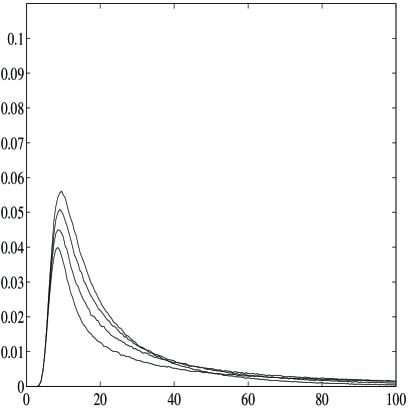
Figure 1: Estimated firing density of the Wiener model with exponentially alternating drift for $\sigma=1$, $\lambda=0.2$, $c=v=1$, with the choices $\mu=0.2,0.3,0.4,0.5$ (bottom to top near the origin).

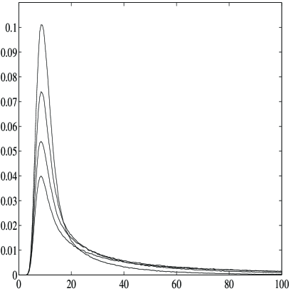
Figure 2: As in Figure 1, with $\sigma=1$, $\mu=0.2$, $c=v=1$, for $\lambda=0.2,0.15,0.1,0.05$ (bottom to top near the origin).

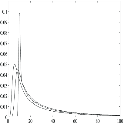
Figure 3: As in Figure 1, with $\lambda=0.2$, $\mu=0.3$, $c=v=1$, for $\sigma=1.8,1,0.2$ (left to right near the origin).

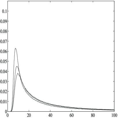
Figure 4: As in Figure 1, with $\lambda=0.2$, $\mu=0.3$, $\sigma=1$, for $c=v=0.8,1,1.2$ (bottom to top near the origin).

6 Erlang distributed inversion times

In this Section we consider the case when the inversion times of the Wiener neuronal model (1) have distribution functions of Erlang type with shape parameter 2: $F_{U}(t)=1-\lambda t\,e^{-\lambda t}$ and $F_{D}(t)=1-\mu t\,e^{-\mu t}$, $t\geq 0$. The mean values of the times intervals separating consecutive inversions of the drift are now given by $2/\lambda$ and $2/\mu$. The analysis has been performed on some cases analogous to those presented in Section 5, with $\mu\geq\lambda$, with threshold $\beta=10$, and with $x_{0}=0$.

As for the case of exponential inversion times, the estimated firing densities are unimodal (see Figures 5$\div$8). Moreover, if $\mu$ increases the median $q_{2}$ decreases, as well as the quartiles $q_{1}$ and $q_{3}$, and the inter-quartile range $IQR$ (see Figure 5). A similar behaviour is again observed if $\lambda$ decreases (see Figure 6). We emphasize that also in this case the firing density becomes less peaked as $\sigma$ increases (see Figure 7). Finally, when $c$ and $v$ increase, with $c=v$, then $q_{1},q_{2},q_{3}$ decrease (see Figure 8). A similar behaviour has also been exhibited by the estimated firing densities in the case of exponentially distributed inversion times (compare Figures 5$\div$8 with Figures 1$\div$4).

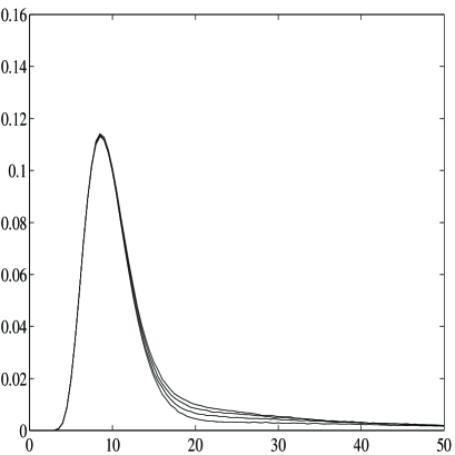
Figure 5: Estimated firing density of the Wiener model with Erlang alternating drift for $\sigma=1$, $\lambda=0.1$, $c=v=1$, for $\mu=0.10,0.15,0.20,0.25$ (bottom to top near abscissa 20).

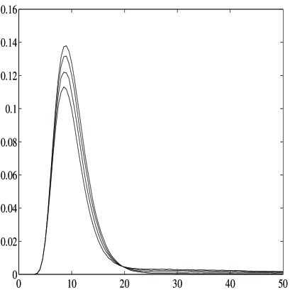
Figure 6: As in Figure 5, with $\sigma=1$, $\mu=0.1$, $c=v=1$, for $\lambda=0.10,0.075,0.05,0.025$ (bottom to top near the origin).

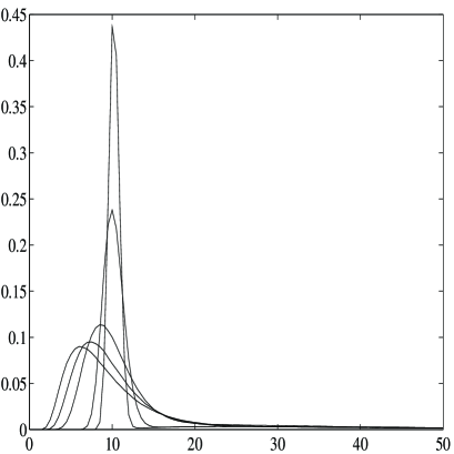
Figure 7: As in Figure 5, with $\lambda=0.1$, $\mu=0.15$, $c=v=1$, for $\sigma=1.8,1.4,1.0,0.4,0.2$ (left to right near the origin).

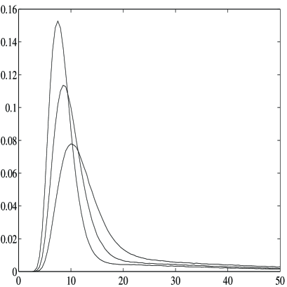
Figure 8: As in Figure 5, with $\lambda=0.1$, $\mu=0.15$, $\sigma=1$, for $c=v=0.8,1,1.2$ (bottom to top near the origin).

7 Deterministic inversion times

With reference to the model (1) let us assume that $c=v$ and that the drift inversion times are deterministic, with $F_{U}(t)=F_{D}(t)={\bf 1}_{\{t\geq\tau\}}$. This means that the second term at the right-hand-side of (1) increases and decreases alternately in a deterministic fashion every $\tau$ instants. In other words,

$$u(t):=\int_{0}^{t}\xi(s)\,{\rm d}s$$ (2)

for $t>0$ is a sawtooth function of period $2\tau$.

As in the previous cases, we have performed $10^{6}$ simulations to obtain estimates of the firing density $g(\beta,t\,|\,x_{0})$, with threshold $\beta=10$ and initial state $x_{0}=0$.

Firing densities now appear to be quite different from the previous cases. Indeed, the estimated firing densities are multimodal. In Figure 9 two examples are shown where the peaks are located near the maxima of (2), i.e. near $\tau,3\tau,5\tau,\ldots\;$.

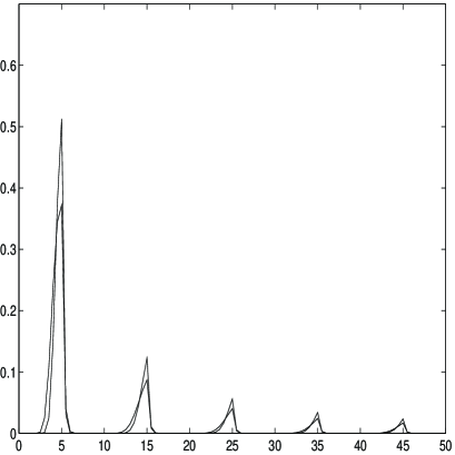
Figure 9: Estimated firing density of the Wiener model with drift alternating at deterministic times for $\tau=5$, $c=v=2$, $\sigma=1$ (lower peaks) and $\sigma=0.7$ (higher peaks).

8 Sinusoidal input

In this Section we shall analyse the effect of a smoother input for the Wiener neuronal model of Section 7 by changing function (2) to a smoother one. More specifically, we assume that the membrane depolarization is now described by the Gauss-Markov diffusion process $\{\hat{X}(t);\,t\geq 0\}$ given by

$$\hat{X}(t)=x_{0}+\int_{0}^{t}\eta(s)\,{\rm d}s+\sigma\,B(t),\quad t\geq 0,$$ (3)

with $x_{0}\in{\bf R}$, $\sigma>0$, and

$$\eta(t)=\alpha\,{\pi\over 2\tau}\,\sin\left({\pi\over\tau}\,t\right),$$

with $\alpha$ and $\tau$ positive. Note that mean and covariance of $\hat{X}(t)$ are given by

$$E[\hat{X}(t)]={\alpha\over 2}\left[1-\cos\left({\pi\over\tau}\,t\right)\right],\quad t\geq 0,$$ (4)

and

$${\rm Cov}[\hat{X}(s),\hat{X}(t)]=\sigma^{2}\,\min\{s,t\},\quad s,t\geq 0,$$

respectively. Hence, $\alpha$ is the maximum value attained by the mean of $\hat{X}(t)$. To compare the present model with that considered in the previous section, we choose the involved parameters in such a way that the functions (2) and (4) possess equal maxima and minima. Hence, according to the parameters’ values chosen in Figure 9 we set $\alpha=c\,\tau$, with $c=v$, $\beta=10$ and $\tau=5$.

To determine the firing density for the model (3) we resort to a numerical procedure due to Di Nardo et al. (2001). The results obtained show that the firing densities are still multimodal (see Figure 10), as for the model described in Section 7, and that the peaks are located around the maxima of (4). The shapes of the firing densities are similar to those obtained for the Wiener model with alternating drift, though being now characterized by less sharp peaks. This is also evident by comparing Figure 10 with Figure 9.

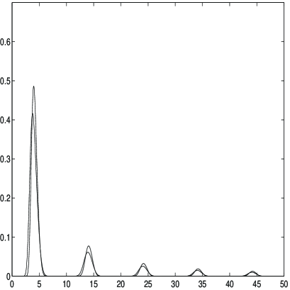
Figure 10: The firing density of the Wiener model with sinusoidal drift for $\tau=5$, $\alpha=10$ $\sigma=1$ (lower peaks) and $\sigma=0.7$ (higher peaks).

9 Concluding remarks

The Wiener neuronal model has been considered by assuming that the effects of alternating stimuli are included into the drift. Making use of a numerical procedure to simulate sample-paths of the resulting process, we have obtained estimates of the firing densities as FPT densities through a constant threshold. Three cases have been considered: the time periods separating consecutive changes of the drift (i) are exponentially distributed, (ii) they have an Erlang-type distribution, and (iii) they possess constant length. For sensible choices of the involved parameters, the results obtained in these three cases are quite different. Indeed, while the presence of randomness in the drift of the process produces unimodal firing densities in cases (i) and (ii), the deterministic behaviour of the drift yields multimodal densities in case (iii). The computational results found in case (iii) have been finally compared with those holding for the Wiener neuronal model subject to oscillating input of sinusoidal type. In this case the firing densities are still multimodal, though less peaked than in case (iii).

References

- [1] Bulsara A.R., Lowen S.B., Rees C.D., 1994. Cooperative behavior in the periodically modulated Wiener process: Noise-induced complexity in a model neuron. Phys. Rev. E, 49, 4989–5000.
- [2] Di Crescenzo A., 2000. On Brownian motions with alternating drifts. In: Cybernetics and Systems 2000 (Trappl R ed.), 324–329. Austrian Society for Cybernetics Studies, Vienna.
- [3] Di Nardo E., Nobile A.G., Pirozzi E., Ricciardi L.M., 2001. A computational approach to first-passage-time problems for Gauss-Markov processes. Adv. Appl. Prob., 33, 453–482.
- [4] Gerstein G.L., Mandelbrot B., 1964. Random walk models for the spike activity of a single neuron. Biophys. J., 4, 41–68.
- [5] Giraudo M.T., Sacerdote L., Sirovich R., 2001. Effects of random jumps on a very simple neuronal diffusion model. In: Abstract book of the 4th International Workshop “Neuronal Coding 2001”, 145. 10-14 September 2001, Plymouth, UK.
- [6] Lánský P., 1997. Sources of periodical force in noisy integrate-and-fire models of neuronal dynamics. Phys. Rev. E, 55, 2040–2043.
- [7] Lánský P., Krivan V., Rospars J.P., 2001. Ligand-receptor interaction under periodic stimulation: a modeling study of concentration chemoreceptors. European Biophys. J., 30, 110–120.
- [8] Plesser H.E., Geisel T., 2001. Stochastic resonance in neuron models: Endogenous stimulation revisited. Phys. Rev. E, 63, 31916–31921.
- [9] Ricciardi L.M., 1995. Diffusion models of neuron activity. In: The Handbook of Brain Theory and Neural Networks (Arbib MA ed.), 299–304. The MIT Press, Cambridge.
- [10] Ricciardi L.M., Di Crescenzo A., Giorno V., Nobile A.G., 1999. An outline of theoretical and algorithmic approaches to first passage time problems with applications to biological modeling. Math. Japonica, 50, 247–322.
- [11] Rubinstein R.Y., 1981. Simulation and the Monte Carlo Method. Wiley, New York.