A long-distance quantum-capable internet testbed

Abstract

Building a Quantum Internet requires the development of new networking concepts at the intersection of frontier communication systems and long-distance quantum communication. Here, we present the implementation of a quantum-enabled internet prototype, where we have combined Software-Defined and Time-Sensitive Networking principles with Quantum Communication between quantum memories. Using a deployed quantum network connecting Stony Brook University and Brookhaven National Laboratory, we demonstrate a fundamental long-distance quantum network service, that of high-visibility Hong-Ou-Mandel Interference of telecom photons produced in two independent quantum memories separated by a distance of 158 km.

I Introduction

Quantum technologies have great potential to enhance information processing, secure communication, and fundamental scientific research Acín et al. (2018). The functional modularity and scalability of Quantum Networks (QNs) make them ideal foundations Simon (2017) to achieve quantum advantage in large distributed quantum processing systems Alsing et al. (2022). Along these lines, realizations, such as Memory-Assisted Measurement Device Independent Quantum Key Distribution (MA-MDI-QKD) Lo et al. (2012), and entanglement distribution using Quantum Repeaters (QRs) Lloyd et al. (2001), will be paramount to establish the Quantum Internet (QI).

The first-generation QI concept was proposed in the late 2000s Kimble (2008), inspired by advancements in network technologies and early light-matter quantum interfaces. The concept is based on interconnected quantum devices, including quantum memories and entanglement sources Awschalom et al. (2021), aimed at distributing quantum entanglement between quantum network nodes. Early demonstrations of this concept have showcased fundamental QN capabilities across short distances, such as direct entanglement distribution Hensen et al. (2016); Valivarthi et al. (2016); Sun et al. (2016); Valivarthi et al. (2020), quantum-state transfer Puigibert et al. (2020); Cao et al. (2020), and interference-mediated entanglement generation between light-matter quantum nodes Slodička et al. (2013). In more recent implementations, efforts are being directed towards scaling similar principles over greater distances using telecom Quantum-Frequency Conversion (QFC) of light generated in quantum light-matter interfaces van Leent et al. (2022); Lago-Rivera et al. (2021); Yu et al. (2020); Neumann et al. (2022).

To enable user-defined QN operations scaled to inter-city distances, a refined QI concept is necessary. This refined QI concept must integrate classical software-defined Xia et al. (2015) and time-sensitive Lo Bello and Steiner (2019) networking principles with QN services Wehner et al. (2018); Pompili et al. (2022), employing a unique stack abstraction merged with classical internet stack elements, thus enabling and enhancing control and operation Fang et al. (2022); Mannalath and Pathak (2022); Chehimi and Saad (2022); Liu et al. (2022); Azuma et al. (2022).

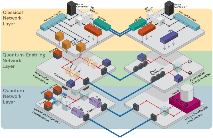
Figure 1: Concept of a stack-driven quantum memory QN, comprising three optical network layers. (Top) A classical control network layer for user-defined control and fast feedback. (Middle) A quantum-enabling network layer supporting time, phase, and polarization analog measurements. (Bottom) A quantum network layer, including room temperature quantum memories, qubit detection systems, and photonic quantum signals transmission.

Here, we present a first realization of such a software-defined quantum network. This Quantum-Enabled Internet Prototype (QEIP) is realized over an inter-city distance of 158km using commercial optical dark fiber connecting controllable quantum nodes available at Stony Brook University (SBU) and Brookhaven National Laboratory (BNL).

The paper is organized as follows: in Section II, we introduce a multi-stack abstraction that delineates the functionalities of the layers comprising our testbed architecture; in Section III, we describe the backbone classical network infrastructure connecting both campuses; in Section IV we detail our long-distance QN, comprising four independent quantum nodes: two nodes with room-temperature quantum memories, performing QFC between the rubidium-resonant near-infrared and telecom wavelengths, and two nodes hosting a measurement station; in Section V we present our polarization compensation and time synchronization systems, which allow the long-distance preservation of the telecom flying qubits; and in Section VI, we describe our novel Quantum Network Control Protocol Suite (QNCPS) and the Application Programming Interfaces (APIs) that enable the execution of elementary QN services. Lastly, in Section VII, we demonstrate the execution of a QN service that includes near-infrared to telecom frequency conversion and inter-node long-distance transmission to demonstrate robust Hong-Ou-Mandel (HOM) interference over different network configurations.

II Experiment-Inspired Hybrid Quantum Internet Concept

Our bottom-up QN design paradigm is guided by the functionalities of the physical hardware forming our testbed. Our QEIP consists of three optical network layers: a quantum layer, a quantum-enabling layer, and a classical layer (see Fig. 1).

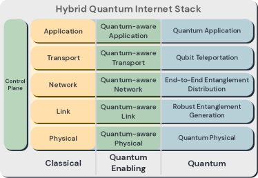
Figure 2: Our envisioned hybrid quantum internet stack. A suite of protocols supports a combination of classical, quantum enabling, and quantum functionalities.

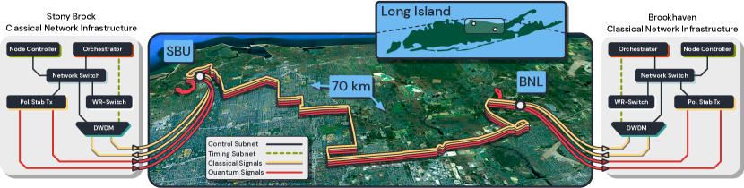
Figure 3: SBU-BNL QN testbed optical infrastructure. Four commercial $\sim$70 km-long optical fibers are used. At SBU, the fiber path runs from the university’s main networking facility (ECC building) to the Physics building’s Quantum Internet Technology laboratory (QIT). At BNL, the fiber path also runs from the main networking facility (ITD building) to the Quantum Information Science and Technology Laboratory (QIST) in the Instrumentation Division building. We utilize dedicated dark fibers (red) for the quantum and the quantum-enabling signals (e.g., the signals for the polarization stabilization system). The time synchronization and data (management/control) signals are carried in a second pair of fibers (green). The Alice and Bob quantum nodes are co-located at SBU with the Charlie measurement station located at BNL. Only the classical and quantum enabling layers of the testbed are shown. Additional fiber loops at SBU and BNL can be added to allow phase independence in the qubit channels. WR = White Rabbit.

1. The Quantum Network Layer comprises interconnected quantum devices where quantum information can be communicated, buffered, and processed. In this work, we focus on the quantum hardware necessary to generate entanglement using robust quantum interference  Cabrillo et al. (1999). We use absorptive atomic quantum memories Lloyd et al. (2001) and demonstrate their compatibility with telecom infrastructure by showing coherent frequency conversion from photons with near-infrared frequency created in the quantum memories (780 nm) to the telecom O-band (1324 nm) (Fig. 1 bottom).
2. The Quantum-Enabling Network Layer prepares long-distance connections to preserve quantum coherence. Core functionality includes supporting time-sensitive operations as well as real-time compensation for environment-induced fluctuations in qubit transmission parameters. We have integrated state-of-the-art long-distance synchronization systems with a temporal resolution below 100 ps, much lower than the temporal envelope of the photons traveling in the network ($\scriptstyle\lesssim$1$\mu$s) Lipiński et al. (2011); Ronen and Lipinski (2015); Dierikx et al. (2016). Additionally, we have implemented feedback mechanisms that preserve the polarization states traveling in single-mode telecom fibers Xavier et al. (2008); Kidoh et al. (1981); Chen et al. (2007) (Fig. 1 middle).
3. Classical Network Layer. State-of-the-art networks use the concepts of Software-Defined Networking (SDN) to realize the management and control of long-distance information transfer and processing Simmons (2014). We have applied similar concepts to our QEIP, where a network of digital devices manages and controls the quantum devices on-demand Khorsandroo et al. (2021). Additionally, we incorporated high-order management concepts to distribute the photons created in the quantum memories across our network topology Sharma et al. (2011); Katramatos et al. (2012) (Fig. 1 top).
4. Hybrid Quantum Internet Stack. The functionality of classical networks is based on a layered software construct, the network stack. This stack implements a suite of protocols that enables end-to-end communication between various connected systems Cer (1983); Illiano et al. (2022). In this work, we implement a hybrid network stack accommodating the quantum-enabling and quantum operations simultaneously Wehner et al. (2018). Conceptually, the components and functionality of our hybrid stack can be separated into three stack protocol sets associated with the role of each optical network described above (see Fig. 2):
a. The quantum stack enables the communication of quantum devices in order to perform the key operations necessary to achieve entanglement generation and distribution Wehner et al. (2018); Pompili et al. (2022) (Fig. 2 right, blue column).
b. The quantum-enabling stack combines the standard TCP/IP stack with time-sensitive principles to establish precise sequences that control quantum devices and compensation systems, allowing for high-fidelity transport of qubits (Fig.  2 center, green column).
c. The classical stack is the standard TCP/IP Kurose and Ross (2022), enabling the interconnection of classical devices controlling the QN (Fig.  2 center, yellow column).
The quantum-aware control plane includes protocols within the classical and quantum-enabling stacks required to control and orchestrate operations at the device, node, domain, and network level (Fig. 2 left, green column).

III Long-Distance Optical Network Testbed Infrastructure

We have built a deployed testbed designed to interconnect quantum nodes over large distances, serving as the foundational infrastructure for implementing the QI hybrid stack concept. Our QEIP testbed interconnects quantum technology laboratories at Stony Brook University (SBU) and Brookhaven National Laboratory (BNL), using four single-mode fiber strands to transmit quantum and classical signals between the two campuses (see Fig. 3). On average, the lab-to-lab loss per fiber strand is $\sim$26dB at 1310nm. The fiber strands have an effective length of approximately 70 km. To randomize the relative phase between the two-qubit channels for HOM interference experiments, we use either a $\sim$20 km fiber loop at the SBU campus for local operations or a $\sim$18 km loop at the BNL campus. This configuration extends the maximum QN distance to approx. 158 km.
Our testbed consists of four QN nodes: Alice and Bob, located at SBU and equipped with independent quantum memory systems (QM). Charlie, situated at BNL, and Dave, located at SBU, host HOM measurement stations. Alice and Bob are connected to Charlie (Dave) through single-mode fibers, each transmitting the photons created in the QMs (red fibers in Fig. 3). The other fibers are used to carry classical signals, allowing for general-purpose data communication (green fibers in Fig. 3). Dense Wavelength Division Multiplexing (DWDM) systems enable multiple independent communication channels. They are used for White Rabbit (WR) protocol connections and to interconnect the primary network switches in each node. Servers and network-compatible electronics are connected to each switch, enabling control operations of the QEIP testbed.

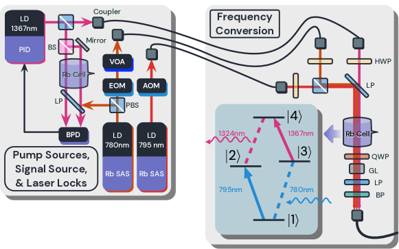
Figure 4: QFC setup. A 780 nm input signal is converted to 1324 nm via FWM with two pumping fields at 795 nm and 1367 nm. An EOM creates the field envelope of $\rm 780nm$ signal. The $\rm 780nm$ signal is combined with the $\rm 795nm$ pump in a polarizing beam splitter and then combined with the $\rm 1367nm$ pump by a long pass filter. A half-wave plate and a quarter-wave plate are used before a GL Polarizer to compensate for birefringence. An $\rm InGaAs$ photodetector is used to detect the generated $\rm 1324nm$ field. The $\rm 1367nm$ laser is locked using an OODR laser stabilization setup. Inset: A diamond atomic scheme is used for frequency conversion. Abbreviations: Laser diode (LD), polarizing beam splitter (PBS), saturated absorption spectroscopy (SAS), quarter/half-wave plate (QWP, HWP), bandpass and longpass filters (BP, LP), Glan laser polarizer (GL).

IV Telecom-Compatible Quantum Network Layer

Our quantum network layer is designed to demonstrate compatibility between our room-temperature quantum memory platform Namazi et al. (2017); Wang et al. (2022) and telecom fiber infrastructure. Specifically, we perform infrared-to-telecom QFC using few-photon-level Four-Wave-Mixing (FWM) in warm atomic vapor.

IV.1 Quantum Frequency Conversion

The QFC setup is based on a four-level diamond atomic system with two pump (classical) fields and two few-photon level (quantum) fields, shown in the inset of Fig. 4. The $\rm 780\leavevmode\nobreak\ nm$ input probe field couples the ground state $\ket{1}$ to the excited state $\ket{3}$. The $\rm 795\leavevmode\nobreak\ nm$ pump I couples the ground state $\ket{1}$ to the excited state $\ket{2}$, and the $\rm 1367\leavevmode\nobreak\ nm$ pump II couples $\ket{3}$ to a higher excited state $\ket{4}$. The QFC process is governed by the following Four-Wave Mixing (FWM) Hamiltonian (see SM for details):

$$\tilde{H} =\hbar\Delta_{a}\hat{a}^{\dagger}\hat{a}+\hbar\Delta_{b}\hat{b}^{\dagger}\hat{b}$$ (1)

$$+\sum^{N}_{i=1}[\hbar\Delta_{2}\sigma^{i}_{22}+\hbar\Delta_{3}\sigma^{i}_{33}+\Delta_{4}\sigma^{i}_{44}+$$

$$(\hbar\frac{\Omega_{I}}{2}\sigma^{i}_{21}+\hbar\frac{\Omega_{II}}{2}\sigma^{i}_{43}+\hbar g_{p}\hat{a}\sigma^{i}_{31}+\hbar g_{QFC}\hat{b}\sigma^{i}_{42}+h.c.)].$$

Here, $N$ is the number of atoms, $\hat{a}^{\dagger}$ is the creation operator of the input probe field, $\hat{b}^{\dagger}$ is the creation operator for the QFC output field connecting states $\ket{2}$ and $\ket{4}$, $\Omega_{I}$ and $\Omega_{II}$ are the Rabi frequencies of the two pumps fields, $g_{p}$ and $g_{QFC}$ are the dipole-coupling strengths for the input and the output quantum fields, $\sigma_{jk}$ is the $jk$ element of the four-dimensional atomic density matrix, and the $\Delta_{i}$’s are the single photon detunings. Using the input-output formalism, one can show that the energy conversion from the $\rm 780nm$ input field to the $\rm 1324nm$ output field follows a linear relation (see SM for the full derivation):

$$\langle\hat{b}_{out}^{\dagger}(t)\hat{b}_{out}(t)\rangle=|G(\omega_{0})|^{2}\,\langle\hat{a}_{in}^{\dagger}(t)\hat{a}_{in}(t)\rangle,$$ (2)

where $|G(\omega_{0})|^{2}$ is a constant conversion efficiency independent of the mean input photon number.

To demonstrate this QFC scheme, the locking of the $\rm 1367nm$ pump is achieved using an Optical-Optical Double Resonance (OODR) scheme in a separate Rb cell. Fig. 4 (top left) shows the atomic level diagram and the OODR setup. We use the $\rm 5S_{1/2}\rightarrow 5P_{3/2}$ transition ($\ket{1}\rightarrow\ket{3}$) at $\rm 780nm$ and the $\rm 5P_{3/2}\rightarrow 6S_{1/2}$ transition ($\ket{3}\rightarrow\ket{4}$) at $\rm 1367nm$. The $\rm 780nm$ optically pumps the $\rm 5P_{3/2}$ level, and it is locked to the $\rm 5S_{1/2}F=3\rightarrow 5P_{3/2}F^{\prime}=4$ transition via saturated absorption spectroscopy (SAS). For OODR, the $\rm 1367nm$ laser is counter-propagating to the 780 nm laser beam in a $\rm 7cm$ rubidium cell maintained at $\rm 60^{\circ}C$. An InGaAs balanced amplified photodetector is used to obtain the OODR spectrum when scanning the $\rm 1367nm$ laser while keeping the 780 nm laser locked. An error signal is generated by modulating the $\rm 1367nm$ laser at $\rm 100kHz$, and the standard Pound-Drever-Hall locking technique is used to stabilize the rubidium telecom frequency.

IV.2 Atomic Quantum Memory Stations at Stony Brook (Alice and Bob)

In the Stony Brook laboratory, we field two identical rubidium vapor quantum memories. They are driven simultaneously to demonstrate the desired QFC (Fig. 4, right). We use two $\rm 71.8mm$ cells at $\rm 100^{\circ}C$ with a natural composition of $\rm{}^{85}Rb$ and $\rm{}^{87}Rb$. We use a diamond configuration in the most abundant $\rm{}^{85}Rb$ isotope. Here, the atomic diamond scheme is constructed using the energy levels $\rm 5S_{1/2},F=3$; $\rm 5P_{1/2},F=3$; $\rm 5P_{3/2},F=4$; and $\rm 6S_{1/2},F=3$ serving as the QFC FWM states $\rm\ket{1},\ket{2},\ket{3},\ket{4}$ respectively, defined in the previous section. The $\rm\hat{a}(t)$ 780 nm probe field and the $\rm\Omega_{II}$ 1367 nm pump field are vertically polarized, while the $\rm\Omega_{I}$ 795 nm pump is horizontally polarized. The two pump fields and the probe qubit $\rm\hat{a}(t)$ beam propagate co-linearly within the atomic vapor. The FWM-generated $\rm\hat{b}(t)$ 1324 nm QFC field is produced with a polarization orthogonal to that of the $\rm\Omega_{II}$ pump field. A Glan Laser Polarizer is used to filter out the vertically polarized $\rm\Omega_{II}$ field, and a band-pass filter($\rm 1320nm$ center wavelength, FWHM $\rm 12nm$) is further used. Finally, the pumps are slightly misaligned from the signal to provide a small spatial separation between the $\rm\Omega_{II}$ pump and the generated $\rm\hat{b}(t)$ beam. Implementing the QNCPS (Section VI.3), we control the $\rm\Omega_{I}$ pump power using an Acousto-Optic Modulator (AOM), and modulate the $\rm\hat{a}(t)$ probe into pulse envelopes using an Electro-Optic Modulator (EOM). This allows us to evaluate the energy conversion efficiency of the all-atomic QFC directly. These measurements are shown in Fig. 5, where the QFC efficiency is determined.

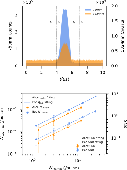
Figure 5: Top: Input and output pulses, detected by the SNSPDs, used to estimate the efficiency of the QFC process. In the cycle time of $10\mu s$, $t_{1}=3\mu s$, $t_{2}=4\mu s$, $t_{3}=6\mu s$ and $t_{4}=7\mu s$. The 1324nm photon number is evaluated within $[t_{2},t_{3}]$ interval and the backgroud noise photon number is evaluated from $[0\mu s,t_{1}]$ and $[t_{4},10\mu s]$. (b) Measured number of photons of QFC pulses at 1324 nm (diamonds) and signal-to-noise ratio (SNR) at the detector (triangles) as a function of the mean photon number in the 780 nm input pulse for Alice (orange) and Bob (blue). The solid and dash lines are linear to the conversion efficiency and SNR curves, respectively. The data comes from calculating mean values after $\sim$20 minutes of interrogation time for pulse repetition rates of 100 kHz. The error bars are dominated by detection and conversion efficiency errors.

The FWM QFC process can be driven with efficiencies higher than 50% Kumar et al. (2023). In our experiments, we achieve a compromise by lowering the QFC efficiency and maximizing the signal-to-noise ratio (SNR), which is the main figure of merit for HOM interference experiments. The conversion efficiencies for the two memories(Alice and Bob) are measured to be $(1.04\pm 0.10)\times 10^{-4}$ and $(1.52\pm 0.05)\times 10^{-4}$. Streams of $\sim 0.9\mu s$ FWHM pulses were used, with Alice’s Pump I operates at 5.20 mW and Pump II at 2.95 mW, while Bob’s Pump I is set to 0.45 mW and Pump II to 2.20 mW. The pulses were detected using Superconducting Nanowire Single-Photon Detectors (SNSPD), and mean photon numbers for the probe and output photons were estimated using the resultant histograms. We then characterized the conversion system by measuring the SNR for different input photon levels (see Fig. 5).

IV.3 Quantum Interference Station at Brookhaven (Charlie) and Stony Brook (Dave)

At the Charlie (Dave) station, active feedback is used to compensate for polarization drifts caused by propagation in the optical fibers (section V.2). Then, the $\rm\hat{b}(t)$ 1324 nm pulses retrieved from the two paths interfere at a $\rm 50:50$ NPBS beamsplitter and then go to two SNSPDs. These detectors generate a signal every time they record a hit. Data is then analyzed to calculate the coincidence rate between the two output arms of the interferometer.

V Long-Distance Quantum-Enabling Network Layer

The successful execution of elementary QN services in our QEIP, such as long-distance HOM interference, requires network-wide clocking finer than the temporal resolution of the QFC-generated photons. Moreover, it also requires continuous tracking of polarization fluctuations and real-time feedback and compensation from the qubit creation to the measurement at the end nodes.

V.1 Distributed Timing and Synchronization

In the context of a HOM indistinguishability QN service, the visibility becomes dependent on the synchronization and temporal jitter of the participating nodes and their protocols. For our quantum memory-based experiments, the temporal bandwidth of the photon qubits is about 500 nanoseconds. To achieve an appropriate degree of timing, we implement the White Rabbit (WR) bidirectional time-transfer technology across the 70 km fiber links connecting the quantum network nodes  Lipiński et al. (2018). Each QN node includes a special-purpose WR timing switch capable of providing 1 PPS and 10 MHz analog synchronization signals. We have measured an upper bound for the time delay between the nodes in our network and calibrated the WR timing switches over the two 70 km fibers, obtaining a time jitter of $100\pm 14$ ps (See Fig. 6 for details).

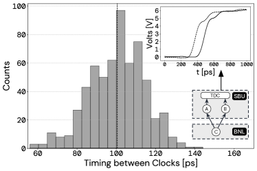
Figure 6: Histogram of jitter events in the 70 km shared clock network, where Charlie (BNL) is the master clock in a tree configuration connecting Alice and Bob (SBU). Bob’s 10 MHz clock shows a delay of $100\pm 14$ ps with respect to Alice’s 10 MHz clock. Inset: Three-node configuration of the White Rabbit devices and sample delay plot between both SBU clocks. TDC: Time Digital Converter.

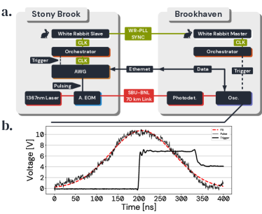
Figure 7: (a) Configuration to measure the long-distance jitter in the shared operation triggers over the 70 km links in the network. (b) Optical pulses are sent from SBU and received at BNL, where the jitter with respect to the local BNL trigger is monitored. Numerical fits to Gaussian curves are used for delay estimations.

We have also characterized the overall QN time jitter, including the driving electronics on the QN nodes. This procedure now involves non-WR coaxial and optical signals being sent between the nodes. Optical pulses are generated at the Stony Brook node using the local SBU WR clock and sent to Brookhaven to be compared with the BNL WR Clock (see Fig. 7). Fig. 8 shows the timing differences between the received pulses and the BNL local trigger over a period of twelve hours. The histogram fits well with a Gaussian distribution with a s.t.d. of $1.45$ ns, well under the temporal bandwidth of the photon pulses. Furthermore, we estimate the Allan deviation $\sigma_{\eta}(\tau)$ (see SM) between the SBU optical signal and the BNL’s WR clock as a function of varying interrogation times in the inset of Fig. 8. We observe the Allan deviation following close a $\tau^{-1/2}$ trend, meaning the jitter between both signals comes from a singular source of white noise. This means that over intervals of less than 12 hours, the noise in our system is predictable. Thus, given our system’s stability and low jitter, we can perform long-distance network protocols requiring stringent timing, such as HOM quantum interference.

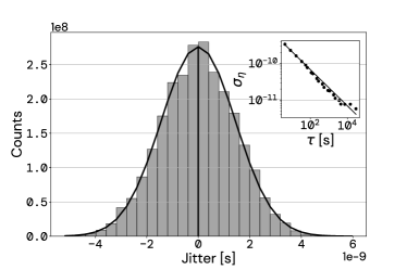
Figure 8: Histogram of jitter events in the SBU-BNL 70 km link after 12 hours of integration time. Inset: Allan deviation associated to the long-distance jitter measurement.

V.2 Polarization Compensation

Polarization stability in our network is doubly essential: Firstly, it allows one to ensure photon indistinguishability predictably, and secondly, it preserves quantum information transmitted across the network as the quantum information is encoded in frequency-converted photon polarization states (PS). Polarization fluctuations present a challenge as we build our long-distance quantum network over the infrastructure used for classical telecommunication networks, which are not designed with polarization stability in mind. In the current optical polarization-agnostic fiber infrastructure, the PS of the light varies along its length due to random birefringence induced by thermal changes, mechanical stress, fiber core irregularities, and other changing environmental and material inhomogeneities Neumann et al. (2022); Bersin et al. (2023).

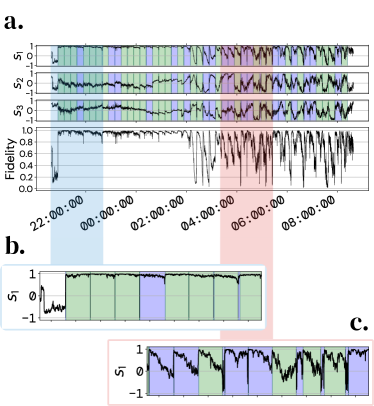
Figure 9: (a) Polarization state, with compensation every 15 minutes (vertical green segments) over one data set of 12 hours between the SBU and BNL nodes, represented with the three normalized Stokes parameters ($S_{1},S_{2},S_{3}$) and Fidelity $F$. Plots (b) and (c) show a clear view of a stable time segment around midnight, and the increased fluctuations for a later time of the day, respectively.

To mitigate such random fluctuations, we perform a dynamic compensation of polarization drifts at each node. Before quantum state transmission between two nodes, we send time-triggered reference macroscopic 1324nm QFC laser light (header) to characterize and compensate for polarization changes. This process is realized by a machine learning-enhanced polarization compensating device built by Qunnect Inc. This device is an early prototype of the now commercially available Qu-APC module and it nullifies any changes to the transmitted light by actively modifying the fiber’s birefringence using motor-controlled fiber loops. Maintaining the polarization of transmitted light ensures the transmitted states’ purity and suitability for HOM interference.

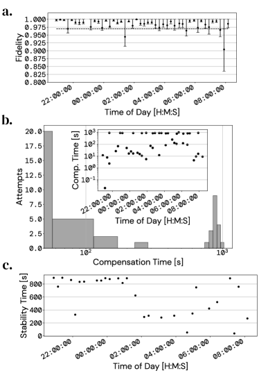
Figure 10: (a) Polarization fidelity measurements with activated feedback every 15 minutes during a collection time of 12 hours. (b) Distribution of the time needed to stabilize/compensate polarization to desired state $\left|H\right>$. Note that no correlation to the time of the day was seen during the 12-hour observation period (inset). (c) Free-drift time for which the polarization fidelity is preserved over $97\%$ (dotted line in (a)) after the compensation is performed.

We run a test over a period of 12 hours, with polarization compensation applied every 15 minutes, to evaluate the polarization fluctuations during the free-running intermediate times and to evaluate the performance of the compensation protocol. Fig. 9 shows a correlation between the stability of the polarization and the time of day. Note that, for example, the most stable time of the day is around midnight, where the PS remains lightly disturbed for almost all of the 15 minutes. This behavior is expected since the optical fiber infrastructure lies along main roads and expressways. Regardless, the active compensation is able to recover the polarization to a fidelity near unity for the majority of the 15-minute free-running time intervals throughout the 12 hours of measurement. Compensation is set to correct the initially horizontally polarized light, with initial Stokes parameters $S^{0}_{1}=1,$ and $S^{0}_{2}=S^{0}_{3}=0$. The Fidelity of the corrected received signal is calculated as $F=\langle H|\hat{\rho}|H\rangle=(1+S_{1})/2$, where $S_{1}$ is the first Stoke parameter (Fig. 9a). The fidelity reached after every compensation step is shown in Fig. 10a.

We evaluated the time needed to perform the polarization compensation (network downtime) and the acceptable free-drift time. Such a characterization is needed to schedule a compensation time sequence during experiments. The compensation time is reported by the polarization compensation device, and it is shown in Fig. 10b. Typical compensation times are between 10 and 100 seconds, and in some cases, high fidelity was not attained at the 15-minute mark. The successful cases are shown with a green background in Fig. 9. The stability time was obtained as the time for when the fidelity has decreased down to $0.97$ after the compensation has been performed (see Fig. 10c). We choose $0.97$ as a preliminary lower bound, assuming two ideal symmetric channels of weak coherent pulses, for a HOM visibility of $\sim\frac{1}{2}f^{2}\approx 0.47$, where $f$ is the fidelity of the channels with respect to each other. We noticed that the fidelity remains slightly affected during the high-stability nighttime, and it usually remains above 200 s most of the time. Based on these results, we activated the polarization compensation protocol after every three-minute interval of free-drift time for the data presented in Section VII. Such a procedure allowed us to attain high HOM visibility during the entire duration of the experiment.

VI Long-Distance Software-Defined Control and Management Layer

On-demand quantum services within a large-scale quantum network, such as HOM interference, also require remote control of devices over the ancillary classical network infrastructure. This classical network distributes the necessary control command sequences responsible for the execution of quantum network operations while also accommodating the traffic necessary for the monitoring and management of the multitude of interconnected devices encompassed in the quantum network.

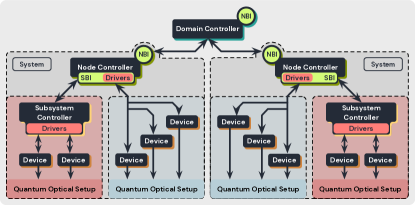
Figure 11: Classical software-defined control network hierarchy concept used to execute quantum network operations on the quantum internet test-bed (two nodes shown). A domain controller orchestrates quantum operations across multiple nodes through their corresponding node controllers’ northbound interface (NBI). Node controllers use their southbound interface (SBI) to drive devices of quantum optical system setups and interface with the controllers of quantum optical subsystems. In a larger-scale internet, multiple domains coordinate to perform quantum operations through orchestrating applications that communicate with domain controllers through their NBI.

Towards the realization of such a control system, we consider - in a bottom-up approach - the hierarchy of control/management software-defined elements acting on signal generation and acquisition hardware, single-photon detectors, polarization compensation systems, and other relevant devices. Starting at the bottom, we distinguish between two types of device organizations: quantum setups and quantum subsystems. Quantum setups refer to configurations of devices requiring direct command sequences from their node controller to operate. Quantum subsystems are operated via an intermediate controller (computer/FPGA) hosting the necessary control software and/or drivers. At the individual node level, a node controller is an entity that coordinates the operations of all node components, either by directly orchestrating ensembles of devices or by interfacing with subsystem controllers to perform operations. The node controller includes northbound Application Programming Interfaces (APIs) to communicate with higher-level (domain) controllers and southbound APIs to interface with quantum subsystems and quantum setups (using drivers for directly interfacing with devices).

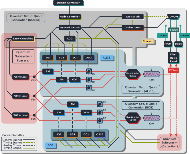
Figure 12: The two co-located controllable quantum memory nodes, Alice and Bob, at the Stony Brook laboratory. The two nodes share the control and timing infrastructure (network and timing switches, node controller, orchestrator, multi-channel arbitrary delay generator - gray background) and the laser subsystem (controllers, 795nm, 780nm, 1367nm lasers, fiber beam splitters to distribute laser light to Alice and Bob - red background), but each has an independent qubit generation quantum optical setup (signal generators, delay controller, variable optical attenuator, beam splitters, feedback oscilloscope, combiner, quantum memory connected to dedicated single-mode long fiber to BNL node - blue background) that includes a quantum memory-based frequency conversion to telecom-friendly 1324nm wavelength within the O-band that enables the signal to reach the BNL node. The detection quantum subsystem (lower right corner) represents the Dave node, identical in functionality to BNL’s Charlie node detector subsystem, and is used for local calibration.

A larger-scale quantum-enabled internet will further encompass multiple such domains that coordinate operations across domains (orchestrators/network managers). Fig. 11 depicts a conceptual scheme of the hierarchy we have adopted in our quantum network testbed.

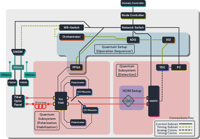
Figure 13: The HOM quantum node, Charlie, at the Brookhaven Laboratory (Dave, at SBU, is identical in functionality) is configured to host the Hong-Ou-Mandel interference experiment setup. One path from the SBU memories is set up to be longer by approximately 18km (20 km) of fiber, going through BNL’s (SBU) local fiber loop infrastructure for phase randomization between channels. Quantum-enabling signals from the two SBU memory nodes are directed to the polarization stabilizer (red background - left). The stabilization system uses computer-controlled mirrors to direct the photons to polarimeters for measurements during the stabilization period. Once the appropriate compensation has been calculated, the mirrors are automatically removed from the path. This allows quantum signals - qubits generated at the SBU memories - to reach the HOM detection setup (red background - right). As is the case with the SBU memory nodes, the control of all components is performed with the node controller and the network switch, while the timing and synchronization with the timing switch, the orchestrator, and the ADG (blue background).

VI.1 Implementation of Long-Distance-Controlled Quantum Nodes

In this section, we describe the first iteration of the full implementation of two types of controllable quantum nodes included in our quantum network testbed. The Alice and Bob nodes on the SBU side of the testbed are qubit generation nodes. On the BNL side, there is a measurement (detecting) node. While the BNL node is stand-alone, for the two SBU nodes, we have taken advantage of the fact that they are co-located and have consolidated the control (classical) network and the timing and driving signal sources. This was done for simplicity as well as space, equipment, and cost considerations. Because the networking systems we use can accommodate multiple channels (wavelengths), the consolidation does not affect the operation of the nodes or the accuracy of the experiments.

Fig. 12 depicts the configuration for SBU. The two nodes share the same network and timing switch, a node controller, a delay trigger controller (orchestrator), and a (multi-channel) Arbitrary Delay Generator (ADG). These systems are shown on a gray background. The nodes also share a laser subsystem (red background). This subsystem includes three lasers, at 795nm, 780nm, and 1367nm, controlled by a dedicated computer running control software. The beam sharing is done using fiber beam splitters. However, each node includes a core quantum configuration (blue background) that independently drives a Quantum Memory (QM) and is connected to its own dedicated fiber that carries the quantum signals to the BNL node. This is done by having the ADG drive two Signal Generators (SGs) and one Delay Controller (DC) per node. The SGs drive Amplitude Modulators (AMs) via acousto-optical devices while the DC drives a Variable Optical Attenuator (VOA). The modulated signal of each laser goes to a beam splitter and a small percentage of it is directed to a detector, which in turn is monitored by an oscilloscope. The oscilloscope readings are used as feedback to optimize the amplitude modulation. The modulated laser signals are combined in an optical setup and then sent to the QM.

Fig. 13 depicts the configuration of the BNL and SBU HOM interference nodes. Here, the qubits generated by the two SBU quantum memories arrive through the long fibers and are directed to an HOM detection subsystem (red background). This setup, along with a polarization stabilization subsystem (also red background), is the key component of these nodes. As with the memory nodes, the control of all components is done with the node controller and the network switch in a central role, while the synchronization is done with the timing switch, the orchestrator, and the ADG (blue background). One optical path from an SBU memory is set up to be longer by approximately 18km (20km) of fiber, going through BNL’s (SBU) local fiber loop infrastructure for dephasing. The first system the photons encounter upon arrival is the polarization stabilizer. The stabilization system uses computer-controlled mirrors to direct the photons to polarimeters for measurements during the stabilization phase. Once the appropriate compensation has been calculated, the mirrors are automatically removed from the path, allowing the photons to go to the HOM detection setup. The HOM setup utilizes two channels of a Superconducting Nanowire Single Photon Detector (SNSPD). The SNSPD is connected to a Time-to-Digital Converter (TDC) supervised by its dedicated PC and driven by an SG. The detector is also connected to the classical network, allowing real-time status monitoring and data acquisition.

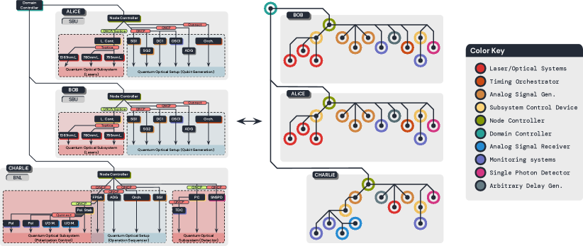
Figure 14: Testbed of Controllable Quantum Nodes: the BNL/SBU testbed has two identical co-located nodes at SBU and a third node at BNL. The left figure shows the devices of each node, color-coded by functionality, their connectivity, and their grouping in quantum optical system setups (blue background) and quantum optical subsystems (red background). The right figure shows a simplified topology and functional representation; each key device of a node is represented with a colored circle; these circles are connected with a hierarchical diagram representing the network connectivity and command/control hierarchy.

VI.2 Network of Controllable Quantum Nodes

As a proof-of-concept, we map our long-distance atomic frequency conversion experiments to the software-defined control paradigm described in the previous section. Furthermore, we establish the process of atomic frequency conversion from near-visible to telecom wavelengths and HOM interference as a quantum network service. Consider the four-node configuration of our network, as mentioned earlier in section III, comprising the Alice, Bob, and Dave nodes at SBU and the Charlie node at BNL. Each quantum node encompasses one or more quantum devices with specific functionality and distinct roles in the operation.

Alice and Bob are identical, both responsible for generating independent sequences of frequency-converted qubits. Each includes one quantum setup and two quantum subsystems: the qubit generation setup and the laser and detector subsystems. The qubit generation setup comprises two signal generators and a configurable power supply (marked in light brown in Fig. 14 (a) and (b)), which drive the electro-optical and acousto-optical devices; the timing infrastructure needed to synchronize the generators to the experiment (White Rabbit) clock; this includes the delay-generator (grey), timing orchestrator (orange), and WR switch (white, not shown for simplicity); and the oscilloscopes (purple), used to auto-calibrate the setup locally. The laser subsystem consists of three lasers at 795nm, 780nm, and 1367nm (marked in red) and their dedicated controller (yellow).

The Charlie node at BNL is the HOM interference detection node. One path from the SBU memories is set up to be longer by approximately 18km of fiber, going through BNL local fiber loop infrastructure for phase randomization between both channels.

Quantum-enabling signals from the two SBU memory nodes are directed to the polarization stabilizer (red background - left). The stabilization system uses computer-controlled mirrors to direct the photons to polarimeters for measurements during the stabilization period. Once the appropriate compensation has been calculated, the mirrors are automatically removed from the path. This allows quantum signals - qubits generated at the SBU memories - to reach the HOM detection setup (red background - right). As is the case with the SBU memory nodes, the control of all components is performed with the node controller and the network switch, while the timing and synchronization with the timing switch, the orchestrator, and the ADG (blue background).

The Dave node at SBU includes a detector configuration identical to Charlie’s detector setup, except that it uses the SBU local fiber infrastructure with a 20 km-long loop. Dave is used for the local calibration of Alice and Bob. All three SBU-located nodes share the classical control and timing infrastructure with no impact in performance.

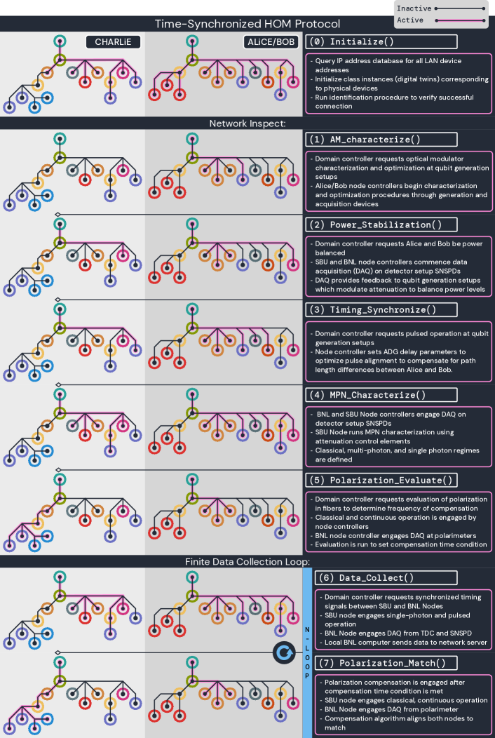
Figure 15: The QNCPS HOM protocol (HOMP) as it applies to a long-distance quantum network. Following the color key of figure 14 (b), the figure describes the sequence of actions necessary to control the experiment.

VI.3 First-Generation Quantum Network Control Protocol Suite

The operation of each quantum node is controlled over the classical network using our Quantum Network Control Protocol Suite (QNCPS). The QNCPS encompasses a set of application layer protocols that exploit the functionality of our hybrid quantum internet stack to orchestrate the operations of various devices over the network infrastructure and enable quantum information flow.

Considering the current structure of our network, as shown in Fig. 14, we take advantage of the fact that all our quantum setups and subsystems are driven and monitored by devices (e,g, signal generators, configurable power supplies, oscilloscopes, time-to-digital converters, etc.) that can be connected to a classical network through standard Ethernet, USB, etc. interfaces. Thus, QNCPS is built upon a series of APIs communicating with device drivers and lower-level software layers to control system elements over the network. These drivers conform to the Virtual Instrument Software Architecture (VISA), an industry-standard API for communicating with instruments over Ethernet, GPIB, and USB interfaces. We have developed a unified API to control devices on top of Python, using Python wrappers for VISA, such as PyVISA. We have implemented the necessary software as a Python package with all associated drivers and built-in search and identification protocols. An essential characteristic of our control API is device agnosticism: it is designed such that higher-level quantum network control protocols do not depend on the make and model of individual devices.

In the present work, we show the implementation of a first instance of a QNCPS protocol as it pertains to HOM interference (HOM Protocol-HOMP). In Fig. 15, we provide a closer look at the interplay between the physical and software layers of the HOMP using the color key shown in figure 14. In this application of the protocol, the software implements a set of 8 primitives executed in 3 phases:

Phase 1: Initialization: Establish communications and put systems on standby.
Initialize(): Domain controller establishes communications with node controllers; directs node controllers to initialize all systems they oversee; node controllers establish communications with all systems and subsystems of their node; lasers are turned on.
Phase 2: Network_Inspect: Confirm nominal operation of all systems. Domain controller instructs node controllers to collect diagnostic information from all systems they oversee and verify good operation.
AM_Characterize(): Characterize amplitude modulators. At Alice and Bob nodes: the node controller executes characterization and optimization sequences for the AMs on the 795nm and 780nm optical lines and maximizes extinction ratios.
Power Stabilization():Balance power levels. Domain controller requests power balancing at Alice and Bob. Node controllers at all three nodes commence Data Acquisition (DAQ) on SNSPDs providing feedback to modulate attenuation.
Timing_Synchronize(): Align pulses. At Alice and Bob nodes: node controller sets ADG delay parameters to optimize pulse alignment to compensate for path length differences between Alice and Bob.
MPN_Characterize(): Find Mean Photon Number (MPN). At Alice and Bob nodes: node controller instructs ADGs to distribute triggers to SGs; switches SGs back to pulsed operation.
At Charlie node: node controller instructs TDC and SNSPD to commence data collection. At Alice and Bob nodes: node controller executes MPN determination sequence for each optical line using feedback from the detector at Charlie over the network; the sequence ramps up the DC power supply that drives the VOA of each node to obtain the desired mean photon number.
Polarization_Evaluate(): Determine polarization compensation parameters. Domain controller instructs node controllers to evaluate the polarization differences between nodes. At Charlie node: node controller activates polarization stabilization subsystem: mirrors are lowered and light is sent to polarimeters. At Alice and Bob nodes: node controller switches SGs to CW operation. At Charlie node: FPGA of stabilization subsystem begins polarization matching process; once completed, compensation and destabilization times are defined.
Phase 3: Data Collection Loop: Collects data within stable polarization time window.
Data_Collect(): Data collection. Domain controller instructs node controllers to perform single-photon level emission and detection. At Alice and Bob nodes: node controller engages single-photon and pulsed operation. At Charlie node: node controller starts detector DAQ, measured data is streamed to network storage.
Polarization_Match(): Match polarizations. Domain controller instructs node controllers to match polarizations between nodes. At Charlie node: node controller activates polarization stabilization subsystem: mirrors are lowered and light is sent to polarimeters. At Alice and Bob nodes: node controller switches SGs to CW operation. At Charlie node: FPGA of stabilization subsystem begins polarization matching process; once completed, data collection resumes.

VII Stack-controlled Long-Distance Quantum Networking Experiments

Having quantum memories capable of QFC at telecom wavelengths and a long-distance fiber infrastructure that preserves the initial quantum states allows us to connect the two quantum light-matter interfaces over long distances. In the following, we describe the first quantum-level experiments performed in our layered QEIP, where we target the observation of long-distance HOM interference using QFC light produced in the quantum memories.

VII.1 Coincidence Counts Distribution for Two-Photon Interference

In order to quantitatively verify the quality of the HOM quantum network service that is being executed in our network testbed, we establish an analytic model for the interference effect between coherent beams. This is especially important in the regime where the bandwidth imposed by pulse modulation is comparable to the beams’ linewidth. The full derivation of our model is laid out in the Supplemental Material (SM); we will exhibit the main results here.

The upper panel of Figure 16 shows a representation of the two coherent beams $\ket{\{\alpha(\nu)\}}$ and $\ket{\{\beta(\nu)\}}$ arriving at the input ports $a$ and $b$ of the final beam splitter, at either Charlie or Dave. These are the quantum states generated in each of the quantum memories and after propagation in the quantum network, as per the lower panel in Fig. 16. We also denote $A(t)$ and $B(t)$ as the Fourier transforms of the spectral functions $\alpha(\nu)$ and $\beta(\nu)$. The states at the output ports $c$ and $d$ are also coherent beams, as shown, with their Fourier transforms also indicated. Note that we are assuming an almost ideal HOM arrangement in that the input and output beams are all in the same, single polarization mode, and the beam splitter is perfectly 50:50, but we allow for the possibility that the arriving beams could have differing intensities.

With that output state defined, we can calculate the rate of expected photon pair detections between ports $c$ and $d$ at times $t_{c}$ and $t_{d}$, respectively. We then project that rate onto each fixed value of $\Delta t\equiv t_{c}-t_{d}$ to identify the pair rate as a function of detection time difference. Following the standard Glauber theory of photo-detection the result is:

$$\frac{dN^{(2)}}{d\,\Delta t} \propto \frac{1}{4}\left(\left(I_{a}+I_{b}\right)\star\left(I_{a}+I_{b}\right)\right)\left(\Delta t\right)$$ (3)

$$-\frac{1}{2}\textbf{Re}\left\{\left(\left(AB^{*}\right)\star\left(AB^{*}\right)\right)\left(\Delta t\right)\right\},$$

where $I_{a}(t)=|A(t)|^{2}$, $I_{b}(t)=|B(t)|^{2}$ are proportional to the two input beam intensities as functions of time, and the $\star$ operation is the cross-correlation functional, e.g. $(F\star G)(\Delta t)=\int F(t+\Delta t)G^{*}(t)dt$.

We can distinguish the first term in Equation 3 as the basic combinatoric rate for two photons being detected from the beams independently, while the second term reflects the HOM interference effect between indistinguishable photons. We can then use Equation 3 to derive the pair rate vs $\Delta t$ pattern for two specific, relevant cases: (i) the continuous-wave (CW) case where the two beam intensities are constant in time, and (ii) the pulsed case, where the two beams are modulated into regularly spaced trains of pulses.

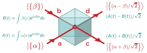
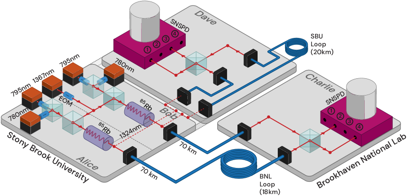
Figure 16: (Upper) General description of the interference of two independent coherent beams. Coherent states $\ket{\{\alpha(\nu)\}}$ and $\ket{\{\beta(\nu)\}}$ are the inputs arriving to the final beam splitter, at Charlie or at Dave. The beams have spectral profiles defined by the frequency-conversion process set during the FWM protocol, as well as pulse-envelope amplitude modulation set by Alice and Bob. The beam splitter output states are also coherent beams, as shown, and we have also shown the Fourier transform of the beams’ spectral functions at each port. (Lower) Overview of the four-node quantum network experiments in this work. Two quantum memories and frequency conversion setups (Alice and Bob) are co-located in the SBU QIT laboratory and are connected independently to the network. The interference setups and telecom-compatible single photon nano-wire detectors (Charlie and Dave stations) are located in the QIST laboratory in BNL and at SBU. Other fibers (not shown) are used to transport classical timing triggers, network status, and sequencing information.

In the CW scenario, all the QFC pumping fields are constant, and the only other relevant information is the spectral shapes of the input beams as they arrive at the beam splitter. Our model assumes the lineshape of the converted 1324 nm beams to be Gaussian, as would be expected from the effects of Doppler broadening in the Rb vapor. We parameterize those lineshapes as Gaussian distributions with standard deviation $\sigma_{\omega}$ over angular frequency $\omega$, and we allow for the possibility that the two beams’ central frequencies could differ by a small amount $\delta\omega$. The pair rate versus $\Delta t$ then follows the form (see the SM for full details):

$$\frac{dN^{(2)}}{d\,\Delta t}\;\propto\;1-\mathcal{V}\;G(\Delta t;0,\sigma_{\omega}^{-1}/\sqrt{2})\;\cos{(\delta\omega\,\Delta t)}\\ ,$$ (4)

where

$$G(t;t_{0},\sigma_{t})\equiv\exp{\left[-\frac{(t-t_{0})^{2}}{2{\sigma_{t}}^{2}}\right]}$$ (5)

is a generic Gaussian form, and $\mathcal{V}\equiv 2I_{a}I_{b}/(I_{a}+I_{b})^{2}$ is the HOM visibility at $\Delta t=0$, which reaches a maximum value of 0.5 in the limit that the two beam intensities are equal. We can interpret the inverse of the RMS in angular frequency $\sigma_{\omega}^{-1}$ as the coherence time of each beam arriving at the beam splitter, which sets the scale for the HOM dip feature versus $\Delta t$; and the $1/\sqrt{2}$ narrowing then reflects the fact that the convolution of two beams has a wider bandwidth and so a shorter coherence time.

We model the case of pulsed beams as simply being CW beams, which are modulated by a time-varying attenuation. In the experiments described below, this is effected by modulating the pump beams driving the FWM process in the QFC memory modules as detailed in Figure 17.

Any modulation in the beams at the beam splitter inputs will necessarily widen their bandwidths, compared to the unmodulated CW beam, so the pulse’s time envelope shape will affect the form of the HOM feature in the pairs distribution over $\Delta t$. We calculate the exact result in the relatively simple case that (i) the beams are pulsed with Gaussian envelopes spaced at regular intervals, (ii) the pulses of the two beams are aligned so their peaks arrive at the beam splitter simultaneously, and (iii) the pulses are well-separated, ie each is short compared to the time interval between them. Assuming the parent, ie pre-modulation, beams are still described by angular frequency linewidths $\sigma_{\omega}$ and frequency difference $\delta\omega$ then the expected form for the pair rate follows as:

$$\frac{dN^{(2)}}{d\,\Delta t}\;\propto\;\left[\sum_{n}G(\Delta t;n\,\Delta T,\sqrt{2}\,\sigma_{t\;pulse})\right]\\ -\mathcal{V}\;G\left(\Delta t;0,\frac{\sqrt{2}\;\sigma_{t\;pulse}}{\sqrt{1+(2\,\sigma_{\omega}\,\sigma_{t\;pulse})^{2}}}\right)\,\cos{(\delta\omega\,\Delta t)},$$ (6)

where $\sigma_{t\;pulse}$ is the RMS of the pulse intensity envelope and $\Delta T$ is the pulse repetition period.

We can see from Equation (6) the essential feature that HOM interference will deplete the pair rate within the “central” peak centered at $\Delta t=0$. In the limit that the pulses are very long compared to the CW beam coherence time, ie, $\sigma_{t\;pulse}\gg\sigma_{\omega}^{-1}$, the modulation does not significantly increase the linewidth at the beam splitter input and we recover the CW result. In the opposite limit, where the pulses are much shorter than the CW coherence time, then the linewidth is completely determined by the pulse modulation and the central peak in the pairs distribution is simply scaled down by a factor of $(1-\mathcal{V})$. Equation 6 spans across the intermediate regime where the pulse width and CW coherence time are comparable; and here, the central lobe of the distribution of the pairs can take on a two-peaked shape, as seen in the data below.

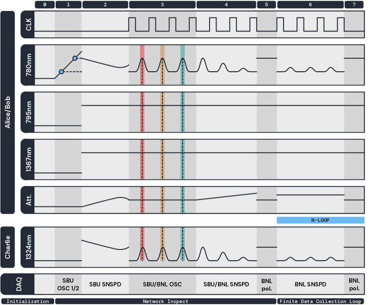
Figure 17: QNCPS/HOMP-driven sequence for quantum memory QFC generation and long-distance HOM interference. Time dynamics of each node and their devices within the network operating the HOMP as in Fig. 15.

VII.2 Experiment I: Stack-Controlled 20 km HOM Two-Photon Interference

The application of the Cabrillo entanglement scheme for our quantum memories Cabrillo et al. (1999) will require close to perfect long-distance HOM interference. Technically, this translates to achieving that the temporal envelope, optical frequency, and polarization of both photon streams produced in the Alice and Bob stations remain indistinguishable at the input of the interference experiment in BNL and SBU.

In our first implementation, we join the concepts of network stack control and pulse operation of the FWM sources in order to perform a Hong-Ou-Mandel measurement of the photons generated in the two memories. We calibrate the relevant parameters of the quantum memories to ensure that Alice and Bob have similar FWM QFC bandwidths and conversion efficiencies. Two independent filtering systems (to filter out the QFC pumps) located after the atomic interfaces, each consisting of several consecutive wavelength filters, are calibrated to have similar transmissions for Alice and Bob. After carefully matching all the auxiliary field parameters, we proceed to frequency convert 780 nm Rb resonant linearly-polarized light at the few-photon level in the two memories and couple their output into the long-distance fibers. The indistinguishability of the independent photon streams is tested using an experimental configuration within the Stony Brook campus, where we use a fiber loop communicating the main Physics building to the CEWIT campus over a distance of 20 km (SBU Loop in Fig. 16), to perform a HOM interference measurement at the Dave node.

These experiments are driven using HOMP to create independent quantum state sequences in each memory. The sequencing is controlled using the network primitives defined in the previous section to achieve: (i) characterization of the 780 nm qubits modulation (using HOMP to drive networked EOMs to produce CW or pulsed states), (ii) verification of QM output mean photon numbers (using HOMP to drive calibrated networked attenuators), (iii) application of QFC pumps to produce 1324 nm photon streams (using HOMP-driven acousto-optical modulators, defining the timing of the telecom pulses), (iv) verification of polarization preservation across the long-distance network (via HOMP-controlled polarization compensation systems), (v) data collection over thousands of production cycles (via HOMP-driven time-to-digital converters and time-taggers collecting the SNSPDs clicks) and (vi) quasi-real time long-distance HOM coincidence analysis (via HOMP-driven servers). Fig. 17 presents the implementation of the HOM quantum network service.

Fig. 18 (inset) shows the result of the HOM quantum network service at the Dave node for a CW input. The mean photon rate was $\sim$ 800 kHz for both Alice and Bob conversion channels at the HOM measurement beam splitter at SBU. The figure also shows the fits of the experimental data to Eq. (4), from which a visibility of 47% can be determined. We note that $\delta\omega\approx 0$ in all the fittings in this work, i.e. both QFC setups were designed to generate same frequency telecom outputs. Fig. 18 (main) shows the result of the HOM quantum network service at the Dave node for a pulsed input. The mean number of photons at the input ports of the HOM BS is $\rm\langle n\rangle\approx$0.04/pulse for both Alice and Bob. The pulse repetition rate was 125 kHz, and a temporal envelope of $\sigma_{t\,pulse}=0.4\,\mu$s was used. The figure also shows the fit of the experimental data to Eq. (6).

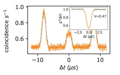
Figure 18: The 1324 FWM HOM quantum interference experiment operates in a stack-controlled regime for the 20 km QEIP configuration at the SBU node. Inset: CW pumps and input probe.

VII.3 Experiment II: Stack-Controlled 158 km HOM Two-Photon Interference

We now demonstrate the degree of indistinguishability of the telecom polarization qubits transduced in two independent quantum memories using HOM interference experiments, with one arm of the interferometer being 70km and the second one being 88km. We mention that the first experiments connecting telecom operational light-matter interfaces and telecom optical links have been shown recently Bock et al. (2018); van Leent et al. (2020); Yu et al. (2020). However, the experiments presented here cover an unprecedented distance.

Fig. 19 top plot shows the result of the HOM quantum network service over 158 km for a pulsed input with a mean number of photons at the output of each memory of $\rm\langle n\rangle_{Alice}=55.5\pm 2.8$ and $\rm\langle n\rangle_{Bob}=9.5\pm 0.5$ defined within one Gaussian pulse temporal envelope FWHM of $\sim 0.9\,\mu s$. The total losses (QM output to SNSPD input) through both the long-distance setups are measured to be $\rm\sim 28.3dB$ for one link and $\rm\sim 36.0dB$ for the longer arm. We obtain an average photon number per pulse, after long-distance propagation, of $\rm\langle n\rangle\approx 0.014$ for both Alice and Bob conversion channels at the HOM measurement beam splitter in BNL. The HOM coincidence rate is measured versus the arrival time of the photons in the two detectors. The coincidences within a temporal region of interest (ROI) are post-selected with a width of 93.4 ns (24 $\mu$s divided in 257 bins). We observe the desired modulation in the coincidence rate, exhibiting a minimum for the initial identical polarization and reaching a maximum corresponding to uncorrelated photons beyond the coherence time of the FWM process. The figure also shows the fits of the experimental data to Eq. (6). An interference HOM visibility is measured to be $\mathcal{V}=(47\pm 4)\%$and an FWM spectral width of $\sigma_{\omega}=(2\pi)\times(609\pm 91)$ kHz. The errors are calculated as the 68% confidence intervals of the fitting curves. Before collecting pulsed HOM data, we verified the HOM setup alignment as a CW HOM service.

Fig. 19 top plot inset shows the result of the HOM quantum network service over 158 km for a CW input with a mean photon rates of $\sim 330$ kHz for both Alice and Bob conversion channel at the HOM measurement beam splitter in BNL. The figure also shows the fits of the experimental data to Eq. (4), from which a HOM visibility of $48\%$ and a bandwidth of $\sigma_{\omega}=(2\pi)\times 453$ kHz can be determined.

The two lower plots are the results of higher photon counts per pulse. The pulse repetition rate was 100 kHz for all three cases, and statistics analysis was carried out with one hour’s worth of integration time for each case. Polarization compensation was performed every three minutes. These results allow us to conclude that our HOM quantum network service works successfully, with the QFC memories and the stack-driven photon distribution successfully preserving the generated quantum states.

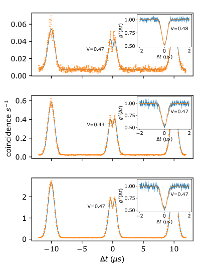
Figure 19: HOM interference measurements operating in a stack-controlled regime for the 158 km QEIP configuration. The measurements are done for different mean photon numbers at the exit of the quantum memories. $\rm\langle n\rangle_{Alice}\sim$ $55.5\pm 2.8$, $182.8\pm 9.2$, $387.5\pm 23.6$ and $\rm\langle n\rangle_{Bob}\sim$ $9.5\pm 0.5$, $31.3\pm 1.6$, $66.4\pm 4.1$. The errors are calculated as the standard deviation of a set of twenty mean values. Each data set corresponds to collecting data for 3 minutes (18 million pulses sent).

VIII Discussion: Towards quantum memory entanglement over hundreds of kilometers

We repeated the HOM quantum network service over 158 km for different input photon numbers per pulse at the output of the QMs. We varied the pulsed output of the frequency conversion to estimated mean number from $\rm\langle n\rangle_{Alice}\sim$ $55.5\pm 2.8$, $182.8\pm 9.2$, $387.5\pm 23.6$ and $\rm\langle n\rangle_{Bob}\sim$ $9.5\pm 0.5$, $31.3\pm 1.6$, $66.4\pm 4.1$. Fig. 19 shows the fits of the experimental data to Eq. (6), showing excellent agreement with the theory for all the data sets.

From the data fits, we obtain the characterization of the quality of the HOM quantum network service. We obtain photon spectrum FWHM widths of $1.4\pm 0.2$ MHz, $1.07\pm 0.06$ MHz, and $1.21\pm 0.06$ MHz, with corresponding photon FWHM pulse widths of $0.92\pm 0.01\,\mu$s, $0.889\pm 0.004\,\mu$s, and $0.880\pm 0.002\,\mu$s, probing the repeatability of the stack-driven HOM quantum network service. Most importantly, we have measured HOM visibilities of $(47\pm 4)$%, $(43\pm 1)$%, and $(47\pm 1$)%, showing that the good visibility of the service is preserved as we approach a true single photon level at the beginning of the communication experiment (Fig. 19). The main data obtained from these measurements are displayed in Table I.

	HOM1	HOM2	HOM3
$\langle n\rangle_{Alice,SBU}$	55 $\pm$ 3	183 $\pm$ 9	387 $\pm$ 24
$\langle n\rangle_{Bob,SBU}$	9.5 $\pm$ 0.5	31 $\pm$ 2	66 $\pm$ 4
$\langle n\rangle_{BS}(\times 10^{-2})$	1.40 $\pm$ 0.07	4.6 $\pm$ 0.2	9.8 $\pm$ 0.6
$\mathcal{V}(\%)$	47 $\pm$ 4	43 $\pm$ 1	47 $\pm$ 1
$R_{coinc}$(Hz)	0.033	0.34	1.48

Table 1: Data from the three sets of pulsed HOM services corresponds to Fig. 19. $\langle n\rangle_{Alice,SBU}$ and $\langle n\rangle_{Bob,SBU}$ are the estimated number of photons per pulse leaving the SBU node. $\langle n\rangle_{BS}$ is the number of photons per pulse of each quantum channel arriving at BNL HOM measurement NPBS input ports. $\mathcal{V}$ is the visibility from the fitting from Eq. (5). $R_{coinc}$ is the coincidence rate at $\Delta t=0$ obtained from the fit. Errors are calculated as the standard deviation of the means of twenty data sets.

From these experimental measurements, we can evaluate the performance of our quantum memory network if we were to apply the original Cabrillo scheme to generate quantum memory entanglement over long distances Cabrillo et al. (1999). The first figure of merit is the long-distance HOM visibility at the single-photon level at the memories sites, which, from the data presented in Table I, can be estimated to be approx. 47%. Assuming that single-photons have the same fidelities as coherent states Michelberger et al. (2015), we would expect a single-photon HOM visibility of 94% for the current level of noise, far surpassing the Peres Horodecki criterion of 33% limit for entanglement generation Peres (1996) and also beyond the 71% CHSH bound to use quantum memory entanglement to perform Bell inequality violation experiments Clauser et al. (1969). The second figure of merit is the two-photon coincidence rate for single-photon-level inputs, which from the data presented at Table I can be estimated to be approx. $4\times 10^{-4}/s$ for the long-distance experiments. This estimation is coherent with the two-photon rate measured in state-of-the-art long-distance quantum memory entanglement experiments Yu et al. (2020); Neumann et al. (2022); van Leent et al. (2022); Luo et al. (2022).

These results make us believe that our current quantum network infrastructure is already capable of performing quantum memory entanglement experiments over unprecedented distances in deployed fibers, contingent on having the QNCPS services running unperturbed over several hundreds of hours. These will be demonstrations one order of magnitude larger than any existing testbed and already nearing the distances where quantum memory advantage can be shown for telecom quantum repeater systems.

IX Outlook

We have presented the design, deployment, and implementation of a first instance of a QEIP network connecting quantum memories over 158 km, in which we demonstrated an elementary quantum network service that of long-distance robust HOM visibility. In order to extend our testbed to execute the network service of entanglement generation among the quantum memories, we envision two major additions. First, we will extend our QFC scheme to generate entanglement with photons directly at 1324 nm and the collective state of the quantum memory. This can be done by correlating the polarization state of the created 1324 photon to that of the resultant intermediate magnetic atomic sublevels Uphoff et al. (2016). Second, after the photon’s propagation in the long-distance links, we will perform a Bell-state projection, thus creating entanglement among the magnetic substates of the quantum memories. This measurement will require phase stabilization across the whole quantum network testbed, which can be achieved by monitoring the long-distance HOM interference shown here Fang et al. (2022).
An additional improvement will be to have long quantum memory coherence times on the order of milliseconds Dideriksen et al. (2021), allowing for the long-distance transmission of the telecom photons and the Bell state result transmission across the quantum-enabling network. With these conditions, it will be possible to verify the entanglement created between the memories by retrieving their state into an entangled photonic state and reconstructing its density matrix.

X Acknowledgments

The authors thank Dr. Olli Sera, Dr. Steven Sagona, and Dr. Mehdi Namazi for their contributions at the early stages of the manuscript. We also thank Prof. Connor Kupchak and Dr. Joanna Zajac for fruitful discussions and comments on the manuscript. Additional thanks to Anthony del Valle and Samuel Woronick for their technical assistance in the later stages of the experiment. This work was supported by the DOE ASCR grant: “Inter-campus network enabled by atomic quantum repeater nodes”, the DOE CESER grant: “A Prototype for Ultimate Secure Transmission”.

Supplementary Materials

Appendix A Theory of quantum frequency conversion in Rubidium

In our quantum frequency conversion system, we are using hot rubidium vapor in a glass cell. We model the system with atomic ensemble in a cavity and apply the input-output theory Gardiner and Collett (1985); Kumar et al. (2023). In the end we go to the bad cavity limit. The Hamiltonian of the system is described as $\hat{H}=\hat{H_{0}}+\hat{H_{L}}$, with the unperturbed Hamiltonian defined as

$$\hat{H_{0}} =\sum^{N}_{i=1}[\hbar\omega_{2}\sigma^{i}_{22}+\hbar\omega_{3}\sigma^{i}_{33}+\hbar\omega_{4}\sigma^{i}_{44}]+\hbar\omega_{a}a^{\dagger}a+\hbar\omega_{b}b^{\dagger}b,$$ (7)

where $i$ represent different atoms in the ensemble. We set the ground state of the atom as the zero energy point. Here $\sigma_{ii}=\ket{i}\bra{i}$, $a$ and $b$ represent 780nm mode and 1324nm mode inside the cavity. The interaction term under dipole approximation takes the form

$$\hat{H_{L}} =\sum_{i}^{N}-\hat{\textbf{d}}^{i}\cdot\textbf{E}=\sum_{i}^{N}-q\hat{\textbf{r}}^{i}\cdot\textbf{E}$$ (8)

In the current four-level Hilbert space (See Fig. 4 in the main text),

$$\hat{\textbf{d}}^{i}=\textbf{d}_{12}\sigma^{i}_{12}+\textbf{d}_{13}\sigma^{i}_{13}+\textbf{d}_{24}\sigma^{i}_{24}+\textbf{d}_{34}\sigma^{i}_{34}+h.c.$$ (9)

where we choose the phase of atomic states $\ket{i}$ so that the dipole matrix element is real. We treat the pump fields as classical fields, and we quantize the two weak fields, such that

E $$=\textbf{E}_{I}+\textbf{E}_{II}+\textbf{E}_{s}+\textbf{E}_{t},\;\textrm{with}$$ (10)

$$\textbf{E}_{I} =\vec{\epsilon}_{I}\frac{\mathscr{E}_{I}}{2}e^{-i\omega^{L}_{I}t+i\vec{k_{I}}\cdot\vec{r}}+c.c.$$

$$\textbf{E}_{II} =\vec{\epsilon}_{II}\frac{\mathscr{E}_{II}}{2}e^{-i\omega^{L}_{II}t+i\vec{k_{II}}\cdot\vec{r}}+c.c.$$

$$\textbf{E}_{s} =\vec{\epsilon}_{s}\mathscr{E}_{s}\hat{a}e^{i\vec{k_{s}}\cdot\vec{r}}+h.c.$$

$$\textbf{E}_{t} =\vec{\epsilon}_{t}\mathscr{E}_{t}\hat{b}e^{i\vec{k_{t}}\cdot\vec{r}}+h.c.$$

where we have assumed the fields propagate in $z$ direction, and

$$\mathscr{E}_{s} =(\frac{\hbar\omega_{s}}{2\epsilon_{0}V})^{1/2}$$ (11)

$$\mathscr{E}_{t} =(\frac{\hbar\omega_{t}}{2\epsilon_{0}V})^{1/2}.$$

Under the rotating wave approximation, we can obtain that

$$\sum_{i}^{N}\hat{\textbf{d}}^{i}\cdot\textbf{E} =\sum_{i}^{N}[\textbf{d}_{12}\cdot\vec{\epsilon}_{I}\frac{\mathscr{E}_{I}}{2}\sigma^{i}_{21}e^{-i\omega^{L}_{I}t+i\vec{k_{I}}\cdot\vec{r}_{i}}+\textbf{d}_{13}\cdot\vec{\epsilon}_{s}\mathscr{E}_{s}\hat{a}\sigma^{i}_{31}e^{i\vec{k_{s}}\cdot\vec{r}_{i}}$$ (12)

$$\ \ \ \ \ +\textbf{d}_{24}\cdot\vec{\epsilon}_{t}\mathscr{E}_{t}\hat{b}\sigma^{i}_{42}e^{i\vec{k_{t}}\cdot\vec{r}_{i}}+\textbf{d}_{34}\cdot\vec{\epsilon}_{II}\frac{\mathscr{E}_{II}}{2}\sigma^{i}_{43}e^{-i\omega^{L}_{II}t+i\vec{k_{II}}\cdot\vec{r}_{i}}+h.c.]$$

$$=-\sum_{i}^{N}[\hbar\frac{\Omega_{I}}{2}\sigma^{i}_{21}e^{-i\omega^{L}_{I}t+i\vec{k_{I}}\cdot\vec{r}_{i}}+\hbar\frac{\Omega_{II}}{2}\sigma^{i}_{43}e^{-i\omega^{L}_{II}t+i\vec{k_{II}}\cdot\vec{r}_{i}}$$

$$\ \ \ \ \ +\hbar g_{s}\hat{a}\sigma^{i}_{31}e^{i\vec{k_{s}}\cdot\vec{r}_{i}}+\hbar g_{t}\hat{b}\sigma^{i}_{42}e^{i\vec{k_{t}}\cdot\vec{r}_{i}}+h.c.],$$

so the full Hamiltonian is

$$\hat{H} =\sum^{N}_{i=1}[\hbar\omega_{2}\sigma^{i}_{22}+\hbar\omega_{3}\sigma^{i}_{33}+\hbar\omega_{4}\sigma^{i}_{44}+(\hbar\frac{\Omega_{I}}{2}\sigma^{i}_{21}e^{-i\omega^{L}_{I}t+i\vec{k_{I}}\cdot\vec{r}_{i}}+\hbar\frac{\Omega_{II}}{2}\sigma^{i}_{43}e^{-i\omega^{L}_{II}t+i\vec{k_{II}}\cdot\vec{r}_{i}}$$ (13)

$$\ \ \ \ \ +\hbar g_{s}\hat{a}\sigma^{i}_{31}e^{i\vec{k_{s}}\cdot\vec{r}_{i}}+\hbar g_{t}\hat{b}\sigma^{i}_{42}e^{i\vec{k_{t}}\cdot\vec{r}_{i}}+h.c.)]+\hbar\omega_{a}a^{\dagger}a+\hbar\omega_{b}b^{\dagger}b$$

We first define the unitary transformation of individual atoms as

$$U_{R}^{i} =e^{-i(\omega_{II}+\omega_{s})t+i(\vec{k_{II}}+\vec{k_{s}})\cdot\vec{r}_{i}}\sigma^{i}_{44}+e^{-i\omega_{s}t+i\vec{k}_{s}\cdot\vec{r}_{i}}\sigma^{i}_{33}+e^{-i\omega_{I}t+i\vec{k}_{I}\cdot\vec{r}_{i}}\sigma^{i}_{22}+\sigma^{i}_{11},$$ (14)

from which we define a global unitary transformation,

$$U_{R} =U^{1}_{R,atom}\otimes U^{2}_{R,atom}...\otimes U^{N}_{R,atom}\otimes e^{-i(\omega_{s}a^{\dagger}a+\omega_{t}b^{\dagger}b)t},$$ (15)

so a state ket transform as $\ket{\tilde{a}}=U_{R}^{\dagger}\ket{a}$. Here $\omega_{I}$ and $\omega_{II}$ are the laser frequency of pump field I and II, while $\omega_{s}$ and $\omega_{t}$ are the frequency corresponds to input signal photon $s$ and output telecom photon $t$. The Hamiltonian transforms as

$$\tilde{H} =U_{R}^{\dagger}\hat{H}U_{R}+i\hbar(\partial_{t}{U_{R}^{\dagger}}U_{R}).$$ (16)

Thus, the full Hamiltonian in the rotating frame takes the form

$$\tilde{H} =\sum^{N}_{i=1}[\hbar\Delta_{2}\sigma^{i}_{22}+\hbar\Delta_{3}\sigma^{i}_{33}+\hbar(\Delta_{4})\sigma^{i}_{44}$$ (17)

$$\ \ \ \ +(\hbar\frac{\Omega_{I}}{2}\sigma^{i}_{21}+\hbar\frac{\Omega_{II}}{2}\sigma^{i}_{43}+\hbar g_{s}\hat{a}\sigma^{i}_{31}+\hbar g_{t}\hat{b}\sigma^{i}_{42}+h.c.)]$$

$$\ \ \ \ +\hbar\Delta_{a}a^{\dagger}a+\hbar\Delta_{b}b^{\dagger}b,$$

where we assumed energy conservation $\omega_{II}+\omega_{s}-\omega_{I}-\omega_{t}=0$ and phase match condition $\vec{k_{t}}+\vec{k_{I}}-\vec{k_{II}}-\vec{k_{s}}=0$. The detunings are defined as $\Delta_{2}=\omega_{2}-\omega_{I}$, $\Delta_{3}=\omega_{3}-\omega_{s}$, $\Delta_{4}=\omega_{4}-\omega_{II}-\omega_{s}$, $\Delta_{a}=\omega_{a}-\omega_{s}$ and $\Delta_{b}=\omega_{b}-\omega_{t}$.

We introduce atomic collective excitation operators, defined as

$$S_{2}^{\dagger} =\frac{1}{\sqrt{N}}\sum_{i}^{N}\sigma^{i}_{21},$$ (18)

$$S_{3}^{\dagger} =\frac{1}{\sqrt{N}}\sum_{i}^{N}\sigma^{i}_{31},$$

$$S_{4}^{\dagger} =\frac{1}{\sqrt{N}}\sum_{i}^{N}\sigma^{i}_{41}.$$

We assume the system is in weak excitation region and the atomic states are always in the symmetric collective excitation manifold. This is a reasonable assumption for atomic state $\ket{3}$ and $\ket{4}$, since input 780nm are of few photon level. This is also a reasonable assumption for state $\ket{2}$, due to the decay channels from $\ket{2}$ to the other ground hyperfine states outside of the four wave mixing loop. With this low excitation assumption the $S_{i}$ operators approximately obey the bosonic annihilation and creation operator commutation relationDuan et al. (2001). Within this symmetric manifold we can also write

$$\sum_{i}^{N}\sigma^{i}_{22} =S^{\dagger}_{2}S_{2}$$ (19)

$$\sum_{i}^{N}\sigma^{i}_{33} =S^{\dagger}_{3}S_{3}$$

$$\sum_{i}^{N}\sigma^{i}_{44} =S^{\dagger}_{4}S_{4}$$

$$\sum_{i}^{N}\sigma^{i}_{43} =S^{\dagger}_{4}S_{3}$$

$$\sum_{i}^{N}\sigma^{i}_{42} =S^{\dagger}_{4}S_{2}.$$

The Hamiltonian is then

$$\tilde{H} =\hbar[\Delta_{2}S^{\dagger}_{2}S_{2}+\Delta_{3}S^{\dagger}_{3}S_{3}+\Delta_{4}S^{\dagger}_{4}S_{4}$$ (20)

$$\ \ \ \ +(\frac{\sqrt{N}\Omega_{I}}{2}S_{2}^{\dagger}+\frac{\Omega_{II}}{2}S^{\dagger}_{4}S_{3}+\sqrt{N}g_{s}\hat{a}S_{3}^{\dagger}+g_{t}\hat{b}S^{\dagger}_{4}S_{2}+h.c.)]$$

$$\ \ \ \ +\hbar\Delta_{a}a^{\dagger}a+\hbar\Delta_{b}b^{\dagger}b$$

The Heisenberg-Langevin equation is Gardiner and Collett (1985); Gardiner and Zoller (2004)

$$\dot{a} =(-\frac{\kappa_{a}}{2}-i\Delta_{a})a-i\sqrt{N}g_{s}S_{3}-\sqrt{\kappa_{a}}a_{in}(t)$$ (21)

$$\dot{b} =(-\frac{\kappa_{b}}{2}-i\Delta_{b})b-ig_{t}S^{\dagger}_{2}S_{4}-\sqrt{\kappa_{b}}b_{in}(t)$$

$$\dot{S_{2}} =(-\frac{\Gamma_{2}}{2}-i\Delta_{2})S_{2}-ig_{t}b^{\dagger}S_{4}-i\sqrt{N}\frac{\Omega_{I}}{2}$$

$$\dot{S_{3}} =(-\frac{\Gamma_{3}}{2}-i\Delta_{3})S_{3}-i\sqrt{N}g_{s}a-i\frac{\Omega_{II}}{2}S_{4}$$

$$\dot{S_{4}} =(-\frac{\Gamma_{4}}{2}-i\Delta_{4})S_{4}-ig_{t}bS_{2}-i\frac{\Omega_{II}}{2}S_{3}$$

where we set input noise terms $S_{i,\ in}(t)=0$. In our experiment we set pump II detuning $\Delta_{2}=0$. It is then reasonable to find steady state by setting $\dot{S_{2}}=0$. Thus we have

$$(-\frac{\Gamma_{2}}{2}-i\Delta_{2})S_{2} =ig_{t}b^{\dagger}S_{4}+i\sqrt{N}\frac{\Omega_{I}}{2},$$ (22)

we also drop the small non linear term. We have

$$S_{2} =\frac{i\sqrt{N}\frac{\Omega_{I}}{2}}{-\frac{\Gamma_{2}}{2}-i\Delta_{2}}=A.$$ (23)

Thus, all nonlinear terms can be eliminated by substitute $S_{2}$, we can write the equation in matrix form

$$\begin{pmatrix}\dot{a}\\ \dot{b}\\ \dot{S}_{3}\\ \dot{S}_{4}\\ \end{pmatrix} =\begin{pmatrix}(-\frac{\kappa_{a}}{2}-i\Delta_{a})&0&-i\sqrt{N}g_{s}&0\\ 0&(-\frac{\kappa_{b}}{2}-i\Delta_{b})&0&-ig_{t}A^{\dagger}\\ -i\sqrt{N}g_{s}&0&(-\frac{\Gamma_{3}}{2}-i\Delta_{3})&-i\frac{\Omega_{II}}{2}\\ 0&-ig_{t}A&-i\frac{\Omega_{II}}{2}&(-\frac{\Gamma_{4}}{2}-i\Delta_{4})\end{pmatrix}\begin{pmatrix}a\\ b\\ S_{3}\\ S_{4}\\ \end{pmatrix}$$ (24)

$$+\begin{pmatrix}-\sqrt{\kappa_{a}}a_{in}\\ -\sqrt{\kappa_{b}}b_{in}\\ 0\\ 0\\ \end{pmatrix}$$

Now we define Fourier transform of the operators in the rotating frame

$$a(\omega^{\prime}) =\frac{1}{\sqrt{2\pi}}\int^{\infty}_{-\infty}dt\ a(t)e^{i\omega^{\prime}(t-t_{0})}$$ (25)

thus in frequency space the above matrix equation becomes

$$\begin{pmatrix}(i\omega-\frac{\kappa_{a}}{2}-i\Delta_{a})&0&-i\sqrt{N}g_{s}&0\\ 0&(i\omega-\frac{\kappa_{b}}{2}-i\Delta_{b})&0&-ig_{t}A^{\dagger}\\ -i\sqrt{N}g_{s}&0&(i\omega-\frac{\Gamma_{3}}{2}-i\Delta_{3})&-i\frac{\Omega_{II}}{2}\\ 0&-ig_{t}A&-i\frac{\Omega_{II}}{2}&(i\omega-\frac{\Gamma_{4}}{2}-i\Delta_{4})\end{pmatrix}\begin{pmatrix}a(\omega)\\ b(\omega)\\ S_{3}(\omega)\\ S_{4}(\omega)\\ \end{pmatrix}$$ (26)

$$=\begin{pmatrix}\sqrt{\kappa_{a}}a_{in}\\ \sqrt{\kappa_{b}}b_{in}\\ 0\\ 0\\ \end{pmatrix}$$

Solving the linear equation, we obtain

$$b(\omega) =\frac{-(-ig_{t}A^{\dagger})(-i\frac{\Omega_{II}}{2})(-i\sqrt{N}g_{s})\sqrt{\kappa_{a}}}{A(\omega)-B(\omega)-C(\omega)-D(\omega)+E(\omega)}a_{in}(\omega),$$ (27)

where

$$A(\omega) =(i\omega-\frac{\kappa_{a}}{2}-i\Delta_{a})(i\omega-\frac{\kappa_{b}}{2}-i\Delta_{b})(i\omega-\frac{\Gamma_{3}}{2}-i\Delta_{3})(i\omega-\frac{\Gamma_{4}}{2}-i\Delta_{4}),$$ (28)

$$B(\omega) =(i\omega-\frac{\kappa_{a}}{2}-i\Delta_{a})(i\omega-\frac{\Gamma_{3}}{2}-i\Delta_{3})(-ig_{t}\frac{-i\sqrt{N}\frac{\Omega_{I}}{2}}{-\frac{\Gamma_{2}}{2}+i\Delta_{2}})(-ig_{t}\frac{i\sqrt{N}\frac{\Omega_{I}}{2}}{-\frac{\Gamma_{2}}{2}-i\Delta_{2}}),$$

$$C(\omega) =(i\omega-\frac{\kappa_{a}}{2}-i\Delta_{a})(i\omega-\frac{\kappa_{b}}{2}-i\Delta_{b})(-i\frac{\Omega_{II}}{2})^{2},$$

$$D(\omega) =(i\omega-\frac{\kappa_{b}}{2}-i\Delta_{b})(i\omega-\frac{\Gamma_{4}}{2}-i\Delta_{4})(-i\sqrt{N}g_{s})^{2},$$

$$E(\omega) =(-ig_{t}\frac{-i\sqrt{N}\frac{\Omega_{I}}{2}}{-\frac{\Gamma_{2}}{2}+i\Delta_{2}})(-ig_{t}\frac{i\sqrt{N}\frac{\Omega_{I}}{2}}{-\frac{\Gamma_{2}}{2}-i\Delta_{2}})(-i\sqrt{N}g_{s})^{2}.$$

In the input-output formalism, the input-output relation is

$$b(\omega) =[b_{out}(\omega)-b_{in}(\omega)]/\sqrt{\kappa_{b}}.$$ (29)

In the conversion system, we only input 780nm as mode $a_{in}(\omega)$ so we can set $b_{in}(\omega)=0$ , the input output relation becomes

$$b_{out}(\omega) =\frac{-(-ig_{t}A^{\dagger})(-i\frac{\Omega_{II}}{2})(-i\sqrt{N}g_{s})\sqrt{\kappa_{a}\kappa_{b}}}{A(\omega)-B(\omega)-C(\omega)-D(\omega)+E(\omega)}a_{in}(\omega).$$ (30)

We define

$$G(\omega) =\frac{-(-ig_{t}A^{\dagger})(-i\frac{\Omega_{II}}{2})(-i\sqrt{N}g_{s})\sqrt{\kappa_{a}\kappa_{b}}}{A(\omega)-B(\omega)-C(\omega)-D(\omega)+E(\omega)},$$ (31)

such that

$$b_{out}^{\dagger}(\omega)b_{out}(\omega) =|G(\omega)|^{2}\ a_{in}^{\dagger}(\omega)a_{in}(\omega).$$ (32)

We will calculate the photon flux operator $b_{out}^{\dagger}(t)b_{out}(t)$ , from which we can obtain the mean photon flux of the output 1324nm signal. By definition

$$b_{out}(t) =\frac{i}{\sqrt{2\pi}}\int^{\infty}_{-\infty}d\omega^{\prime}\ b_{1}(\omega^{\prime})e^{-i\omega^{\prime}(t-t_{1})},$$ (33)

where $b_{1}(\omega)$ is understand to be field operator $b_{\omega}$ outside the cavity at $t=t_{1}$ in the future time.

$$a_{in}(t) =\frac{i}{\sqrt{2\pi}}\int^{\infty}_{-\infty}d\omega^{\prime}\ a_{0}(\omega^{\prime})e^{-i\omega^{\prime}(t-t_{0})},$$ (34)

where $a_{0}(\omega)$ is understand to be field operator $a_{\omega}$ outside the cavity at $t=0$. Comparing the definition and the operator Fourier transform, we have

$$a_{in}(\omega) =ia_{0}(\omega)$$ (35)

$$b_{out}(\omega) =ie^{i\omega(t_{1}-t_{0})}b_{1}(\omega),$$

however, we usually use the annihilation and creation operator in normal order, they always appear in conjugate pairs, so

$$a^{\dagger}_{in}(\omega)a_{in}(\omega) =a^{\dagger}_{0}(\omega)a_{0}(\omega)$$ (36)

$$b^{\dagger}_{out}(\omega)b_{out}(\omega) =b^{\dagger}_{1}(\omega)b_{1}(\omega).$$

Also, by definition of the Fourier transform,

$$b_{out}(t) =\frac{1}{\sqrt{2\pi}}\int^{\infty}_{-\infty}d\omega^{\prime}\ b_{out}(\omega^{\prime})e^{-i\omega^{\prime}(t-t_{0})},$$ (37)

so we can write

$$\langle b_{out}^{\dagger}(t)b_{out}(t)\rangle =\frac{1}{2\pi}\int^{\infty}_{-\infty}\int^{\infty}_{-\infty}d\omega_{1}d\omega_{2}\ e^{-i(\omega_{2}-\omega_{1})(t-t_{0})}G^{*}(\omega_{1})G(\omega_{2})\langle a_{0}^{\dagger}(\omega_{1})a_{0}(\omega_{2})\rangle$$ (38)

The LHS is exactly the mean photon flux at time $t$. To find out conversion efficiency, in our case we note that contribution of $\langle a_{0}^{\dagger}(\omega_{1})a_{0}(\omega_{2})\rangle$ only comes from near center frequency $\omega_{0}$ , so we make the narrow-bandwidth approximation that

$$\langle b_{out}^{\dagger}(t)b_{out}(t)\rangle =G^{*}(\omega_{0})G(\omega_{0})\frac{1}{2\pi}\int^{\infty}_{-\infty}\int^{\infty}_{-\infty}d\omega_{1}d\omega_{2}\ e^{-i(\omega_{2}-\omega_{1})(t-t_{0})}\langle a_{0}^{\dagger}(\omega_{1})a_{0}(\omega_{2})\rangle$$ (39)

$$=|G(\omega_{0})|^{2}\langle a_{in}^{\dagger}(t)a_{in}(t)\rangle,$$

thus the conversion efficiency is $|G(\omega_{0})|^{2}$. In the weak excitation region, this conversion efficiency is independent of the input photon number. In our experimental setup, $\Delta_{2}=\Delta_{3}=\Delta_{4}=0$, and $\Delta_{a}=\Delta_{b}=0$. In the limit of free-space coupling, i.e. very broadband cavity (large $\kappa_{a}$ and large $\kappa_{b}$), we can approximate the conversion efficiency as

$$|G(0)|^{2}=\left|\frac{4Ng_{s}\,g_{t}\,\Omega_{I}\,\Omega_{II}}{\Gamma_{2}\left(\Omega_{II}^{2}+\Gamma_{3}\,\Gamma_{4}/2\right)}\right|^{2}\frac{1}{\kappa_{a}\kappa_{b}}.$$ (40)

Appendix B Allan Deviation

We define the normalized jitter as $\eta_{i}=1+f_{R}\times t_{i}$, where $f_{R}=10$ kHz is the pulsing repetition rate and $t_{i}$’s are the jitter measurements. We define the Allan variance as

$$\sigma^{2}_{\eta}(\tau)=\frac{1}{2(M-1)}\,\sum_{k=1}^{M-1}\left(y_{k+1}-y_{k}\right)^{2},$$ (41)

where $y_{k}=(1/L)\sum_{i=1}^{L}\eta_{(k-1)L+i}$, $k=\{1,2,...,M\}$, $L$ is the number of data points in each segment of interrogation time $\tau$, $L=\tau f_{R}$, $T=M\tau$, and $N=ML$. $T$ is 12 hours and $N$ is the total number of collected data points.

Appendix C HOM Interference Model

C.1 Setup and notation

We are considering the situation pictured in Figure 20, where two independent coherent beams are incident on the input ports $a$ and $b$ of a standard (ie ideal 50:50, non-polarizing) beam splitter; and we want to calculate the rate of coincidences observed at the two output ports $Y$ and $d$ as a function of two specific measurement times $t_{c}$ and $t_{d}$. Our main goal is to calculate what the shape of this coincidence rate looks like versus the arrival time difference $\tau\equiv t_{c}-t_{d}$. In the case of CW beams this will show us the HOM interference dip, and we will then consider the case of the beams being pulsed in time.

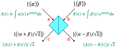
Figure 20: Generic setup for interference of two independent coherent beams; see text for details.

C.1.1 Initial beam states

We assume the incoming beams each come from a laser with a small but finite range in frequencies, or linewidth. Each individual mode $k$ within the beam is then assumed to be in a coherent state, which is typically denoted with a single lower-case Greek letter, i.e. $\ket{\alpha}_{k}$. Such coherent states can be expanded in terms of a Fock number state basis, but for our purposes the only thing we need to know is that a coherent state is an eigenstate of the lowering or annihilation operator of a coherent state as proposed by Glauber back in 1963. For that mode:

$$\hat{a}_{k}\ket{\alpha}_{k}=\alpha\ket{\alpha}_{k}$$ (42)

Here $\alpha$ can be any dimensionless complex number, and its phase encodes the phase of the that mode’s oscillating electric field while its magnitude encodes the number of photons in the mode across the entire quantization time interval. Now we imagine that the beam has non-zero intensity over some range of modes, and so each mode gets its own complex amplitude number $\alpha_{k}$. The set of all these amplitudes ${\alpha}$ then completely defines the beam, and the standard notation for the state of the field in the beam is $\ket{\{\alpha\}}$ as shown entering at point $a$ in Figure 20. When we picture using a quantization volume, and so a discrete set of states $k$, the $\alpha_{k}$ can be encoded as a function $\alpha()$ defined at each discrete frequency $\nu_{k}$, e.g. $\alpha(\nu_{k})=\alpha_{k}$; and we will continue this function to a continuous function $\alpha(\nu)$ to represent the beam.

If we assign $\alpha$ to describe the beam entering at port $a$, and a corresponding spectral function $\beta(\nu)$ for the beam at port $b$, as in Figure 20, then we can write the complete incoming state very simply as

$$\ket{\Psi}_{a,b}=\ket{\{\alpha\}}_{a}\otimes\ket{\{\beta\}}_{b}$$ (43)

C.1.2 Intensity, transforms and coherence time: Weiner-Khinchin interlude

Following the general Glauber theory of photo-detection we can write the intensity in any beam, ie the average number of detectable photons per time interval at one location, for a field with state $\ket{\Psi}$ at any given time $t$ as

$$I(t)\equiv\frac{dN}{dt}=\int\frac{dN}{d\nu\,dt}d\nu\,\propto\,\bra{\Psi}\hat{\mathcal{E}}^{(-)}(t)\,\hat{\mathcal{E}}^{(+)}(t)\,\ket{\Psi}=\left|\,\hat{\mathcal{E}}^{(+)}(t)\,\ket{\Psi}\right|^{2}$$ (44)

Here $\hat{\mathcal{E}}^{(+)}(t)$ is the positive-frequency electric field operator at a particular location, which we can be written easily, at least up to a proportionality, in terms of mode annihilation operators $\hat{a}_{k}$:

$$\hat{\mathcal{E}}^{(+)}(t)\;\propto\sum_{k}\hat{a}_{k}\;e^{+i\,\nu_{k}\,t\,2\pi}\propto\int\hat{a}_{\nu}\,e^{+i\nu t2\pi}d\nu$$ (45)

and of course $\hat{\mathcal{E}}^{(-)}(t)$ is its adjoint. Applying this to our beam with state $\ket{\Psi}=\ket{\{\alpha\}}$ and using the coherent state property in Equation 42 yields the simple result

$$I(t)\propto\left|\,\sum_{k}\alpha(\nu_{k})\;e^{+i\,\nu_{k}\,t\,2\pi}\,\right|^{2}\propto\left|\,\int\alpha(\nu)\,e^{+i\nu t2\pi}d\nu\,\right|^{2}$$ (46)

This makes it natural to define the Fourier transform of $\alpha(\nu)$, which we will denote as $A(t)$

$$A(t)\equiv\mathcal{F}^{-1}\left[\alpha(\nu)\right](t)\equiv\int\alpha(\nu)\,e^{+i\nu t2\pi}d\nu\quad\text{and so}\quad I(t)\propto\left|A(t)\right|^{2}$$ (47)

as is also shown in channel $a$ of Figure 20. We will use Equation 47 to define our convention for an inverse Fourier transform, ie from frequency to time, with the forward transform then being

$$\alpha(\nu)=\mathcal{F}\left[A(t)\right](\nu)\equiv\int A(t)\,e^{-i\nu t2\pi}dt$$ (48)

and so refer to the two as a Fourier transform pair, denoted

$$A(t)\stackrel{{\scriptstyle\mathcal{FT}}}{{\leftrightarrow}}\alpha(\nu)$$ (49)

As in a semi-classical treatment – most appropriate here since coherent states correspond most closely to classical EM waves – we can think of $A(t)$ as describing the oscillating electric field at one point at time $t$, where its magnitude is the field amplitude and its complex phase is the phase of the oscillation. For a CW laser beam we would expect $|A(t)|$ to be quite constant, but we can see from Equation 47 that its phase will change in an almost random way over time. One definition of coherence is to say that if you know the phase at one point in time you can predict it at another point in time, so we can ask: how well correlated is the phase of $A(t)$ between two times? The longest time interval for which the correlation is significant is the then coherence time for that beam, which we will find is directly, and inversely, related to the linewidth.

To measure how well a function is correlated with itself at a certain interval, or lag, we calculate the cross-correlation of the function with itself, or simply its auto-correlation:

$$\text{Autocorrelation}\left[A(t)\right](\Delta t)\equiv(A\star A)(\Delta t)\equiv\int A(t^{\prime}+\Delta t)A^{*}(t^{\prime})dt^{\prime}$$ (50)

The autocorrelation will have a maximum, positive value at $\Delta t=0$ where it is just the total integral of the intensity $|A(t)|^{2}$, and then will fall off toward zero when $\Delta t$ is larger than the coherence time (by definition).

Autocorrelations have many useful properties, and we can derive one of the most important simply by substituting the definition of $A$ in terms of $\alpha$ from Equation 47

$$(A\star A)(\Delta t)=\int\left(\int\alpha(\nu^{\prime})e^{+i\;\nu^{\prime}\;(t^{\prime}+\Delta t)\;2\pi}d\nu^{\prime}\right)\left(\int\alpha^{*}(\nu^{\prime\prime})e^{-i\;\nu^{\prime\prime}\;t^{\prime}\;2\pi}d\nu^{\prime\prime}\right)dt^{\prime}$$ (51)

We leave it as an exercise for the reader to show that this reduces to

$$(A\star A)(\Delta t)=\int\left|\alpha(\nu^{\prime})\right|^{2}e^{+i\;\nu^{\prime}\;\Delta t\;2\pi}d\nu^{\prime}=F^{-1}[\left|\alpha(\nu)\right|^{2}](\Delta t)$$ (52)

We recognize $\left|\alpha(\nu)\right|^{2}$ as the density of photons in the beam per unit frequency, over the whole quantization interval, also called the number spectral density $dN/d\nu$ or simply the lineshape function. The result of Equation 52, then, is that the autocorrelation of a time series is the Fourier transform of that series’ spectral density function. This is known as the Weiner-Khinchin theorem and forms a bedrock result of signal processing theory.

This also reveals the general relationship between linewidth and coherence time, as mentioned above. For smooth, single-peaked functions, as simple laser lineshapes will tend to be, the width of a function and the width of its Fourier transform will be inversely related. For Gaussians the relation is exact between RMS widths; for more general functions the general rule holds, that beams with larger linewidth (or bandwidth) will have shorter coherence times while beams with narrower/smaller linewidths will have longer coherence times.

C.2 Pair Rates and Coincidence Distribution

Looking back now to Figure 20 we describe the input beam at point $a$ with the spectral function $\alpha(\nu)$, which has transform $A(t)$, and the input beam at point $b$ has spectral function $\beta(\nu)$, and corresponding transform $B(t)$. After writing the output state, which is almost trivial in this case, we will calculate the rates for observing pairs at the outputs, and then consider both the case of CW beams and envelope-pulsed beams.

In general, higher Fock states do not pass smoothly through beam splitters. A perfectly simple, well-defined energy eigenstate with occupation number $n$ will result in an output state that is a superposition of some number $m$ photons having come out one side and $k$ out the other, for all possible combinations of $m+k=n$. As a general procedure it will be simpler, then, to propagate the operators at the output locations back to the input locations, than it is to move the input state to the output state.

However, coherent states are very much the exception to this rule. As might be expected from the counterpart to classical EM waves a coherent state at a beamsplitter input is simply transformed into two coherent states, one at each output. Specifically, for a coherent state defined by $\ket{\{\alpha\}}_{\mathrm{Input}}$ at the input to a 50:50 symmetric beamsplitter the state of the two outputs is $\ket{\{\alpha/\sqrt{2}\}}_{\mathrm{Out1}}\otimes\ket{\{\alpha/\sqrt{2}\}}_{\mathrm{Out2}}$. We can see that this evolution conserves energy, while both beams and inherit the same phase relation between modes as in the original beam.

With two input beams we can simply add their amplitudes at the two outputs, keeping in mind that one of them has to be phase-reversed (this is needed to conserve energy and so a general property of beam splitters). The net result is shown in the lower half of Figure 20, where the states of the output beams at port locations $c$ and $d$, and their transforms, are

$$\ket{\Psi}=\ket{\{(\alpha+\beta)/\sqrt{2}\}}_{c}\otimes\ket{\{(\alpha-\beta)/\sqrt{2}\}}_{d}$$ (53)

$$\left(A(t)+B(t)\right)/\sqrt{2}\quad\text{at c and}\,\,\left(A(t)-B(t)\right)/\sqrt{2}\quad\text{at d}$$ (54)

With this we can write the rate for two-photon observations at ports $c$ and $d$, specifically at times $t_{c}$ and $t_{d}$ as

$$\frac{d^{2}N^{(2)}}{dt_{c}\;dt_{d}}\propto\left|\hat{\mathcal{E}}^{(+)_{c}}(t_{c})\;\hat{\mathcal{E}}^{(+)_{d}}(t_{d})\ket{\Psi}\right|^{2}\\$$ (55)

Substituting Equations 45 and 53 into the above then yields

$$\frac{d^{2}N^{(2)}}{dt_{c}\;dt_{d}} \propto \frac{1}{4}\left|\int(\alpha(\nu^{\prime})+\beta(\nu^{\prime}))e^{+i\,\nu^{\prime}t_{c}\,2\pi}d\nu^{\prime}\int(\alpha(\nu^{\prime\prime})-\beta(\nu^{\prime\prime}))e^{+i\,\nu^{\prime\prime}t_{d}\,2\pi}d\nu^{\prime\prime}\;\right|^{2}$$ (56)

$$= \frac{1}{4}\left|\left(A(t_{c})+B(t_{c})\right)\left(A(t_{d})-B(t_{d})\right)\right|^{2}$$

Expanding Eq. 56 gives us three types of terms:

• Balanced, synchronous terms which contain only combinations of products $A()\,A^{*}()$ and/or $B()\,B^{*}()$ with both paired factors evaluated at the same time. These terms are immediately real and correspond to products of the beam intensities, see below.

• Balanced, asynchronous terms containing $A()\,A^{*}()$ and $B()\,B^{*}()$ products which are evaluated at differing times. These terms are where the interference effects will stem from.

• Unbalanced terms, where at least one factor of $A$ or $B$ is not balanced by its complex conjugate. These terms will have a very fast varying phase at all times and will vanish in any time integration such as we are about to carry out in Equation 59 below.

If we drop the unbalanced terms then Eq. 56 can be re-arranged to

$$\frac{d^{2}N^{(2)}}{dt_{c}\;dt_{d}} \propto \frac{1}{4}\left[I_{a}(t_{c})I_{a}(t_{d})+I_{b}(t_{c})I_{b}(t_{d})+I_{a}(t_{c})I_{b}(t_{d})+I_{b}(t_{c})I_{a}(t_{d})\right]$$ (57)

$$\quad-\frac{1}{2}\;\textbf{Re}\left\{A(t_{c})B^{*}(t_{c})B(t_{d})A^{*}(t_{d})\right\}$$

where we have identified the single-photon intensities in the two incoming beams very naturally as $I_{a}(t)\equiv|A(t)|^{2}$ and $I_{b}(t)\equiv|B(t)|^{2}$.

The result of Equation 57 admits a simple and pleasing interpretation, namely: (i) The first line of the RHS is the “combinatoric” pair rate, corresponding to the purely classical product of the probabilities of getting individual photons from the single beams; the first two terms are the rates for two photons from one beam, the latter one photon from each beam; and (ii) The second line is then the “interference” term embodying the HOM effect and always involves both beams; and, note that the intereference term is strictly negative. Further, a little thought will show that the interference term will only be significant if the time difference $\Delta t=t_{d}-t_{c}$ is on the order of, or smaller than, the beams’ coherence time.

For the experiment we have in mind we want to integrate the number of observed pairs over time, binned on the time difference between the detections. Accordingly we will change variables from $[t_{c},t_{d}]$ to $[\,t_{c},\,\Delta t\equiv t_{d}-t_{c}]$ and then integrate the pair rate over all $t_{c}$

$$\frac{dN^{(2)}}{d\,\Delta t} = \int\frac{d^{2}N^{(2)}}{dt_{c}\;d\Delta t}dt_{c}$$ (59)

$$\propto \frac{1}{4}\int\left[I_{a}(t_{c})I_{a}(t_{c}+\Delta t)+I_{b}(t_{c})I_{b}(t_{c}+\Delta t)+I_{a}(t_{c})I_{b}(t_{c}+\Delta t)+I_{b}(t_{c})I_{a}(t_{c}+\Delta t)\right]dt_{c}$$

$$\quad-\frac{1}{2}\int\;\textbf{Re}\left\{A(t_{c})B^{*}(t_{c})B(t_{c}+\Delta t)A^{*}(t_{c}+\Delta t)\right\}\,dt_{c}$$

We can recognize the integral of each of the product terms in Equation 59 as having the form of either an auto-correlation or cross-correlation. Keeping in mind that we can exchange the order of integration and the $\textbf{Re}\{\}$ operation this then simplifies to the pleasingly compact form in terms of just two autocorrelations:

$$\frac{dN^{(2)}}{d\,\Delta t} \propto \left[(I_{a}\star I_{a})(\Delta t)+(I_{b}\star I_{b})(\Delta t)+(I_{a}\star I_{b})(\Delta t)+(I_{b}\star I_{a})(\Delta t)\right]$$ (60)

$$\quad-\frac{1}{2}\textbf{Re}\left\{\int A(t_{c})B^{*}(t_{c})B(t_{c}+\Delta t)A^{*}(t_{c}+\Delta t)\,dt_{c}\right\}$$

$$= \frac{1}{4}((I_{a}+I_{b})\star(I_{a}+I_{b}))(\Delta t)-\frac{1}{2}\textbf{Re}\left\{((A\,B^{*})\star(A\,B^{*}))(\Delta t)\right\}$$

While arguably elegant overall, the form of Equation 60 is not fully practical: the first, combinatoric term follows just from the beams’ power envelopes, but the second, interference term is not yet connected to measurable properties of the individual beams. To make further progress we need to specify more about the those properties. We will look at the case for CW beams in Section C.3 next, and then the more general case of envelope-pulsed beams in SectionC.4 that follows.

C.3 Interference dip, CW case

The simplest case to analyze is when both incoming coherent beams are macroscopically structureless, ie constant intensity or CW; and the frequency spread of the beam is relatively small, say much less than one octave, and their spectral distributions are smooth. In this case the intensities $I_{a},I_{b}$ will be constant and the only structure in the pair rate vs $\Delta t$ will come from the interference term. But the only physical parameters that define the two beams are their lineshapes: for a narrow-band beam the different frequency components will fall out of phase with one another, making the sum phase at any given time effectively random. Thus we expect to see that the interference term can be expressed purely in terms of the two beam’s spectral density functions, or lineshape functions, which we know to be $|\alpha(\nu)|^{2}$ and $|\beta(\nu)|^{2}$.

Our first step will be to re-cast the interference term using $\alpha$ and $\beta$ instead of $A$ and $B$. Concentrating on just the argument of the $\textbf{Re}\{\}$ operator in Equation 60, after a bit of prestidigitation we can arrive at

$$((A\,B^{*})\star(A\,B^{*}))(\Delta t)=\mathcal{F}^{-1}\left[\,\left|(\alpha\star\beta)(\nu)\right|^{2}\right]$$ (61)

(We leave it as an exercise for the diligent reader to derive this result; one can go the long way following direct substitution, or pull a trick by using the Weiner-Khinichin theorem again first.)

Equation 61 looks very promising, since we have a convolution of the two spectral functions as the central ingredient. But this is still not operational, since we only know the amplitude structure of $\alpha(\nu)$ and $\beta(\nu)$ and not their phase structure. To highlight this let’s call out the phase and amplitudes separately for each:

$$\alpha(\nu)\equiv|\alpha(\nu)|\,e^{i\phi_{\alpha}(\nu)}\quad\text{and}\quad\beta(\nu)\equiv|\beta(\nu)|\,e^{i\phi_{\beta}(\nu)}$$ (62)

Now we can re-write the core of Equation 61 vis

$$\left|(\alpha\star\beta)(\nu)\right|^{2} = \left|\int\alpha(\nu^{\prime})\beta^{*}(\nu^{\prime}+\nu)d\nu^{\prime}\right|^{2}$$ (63)

$$= \int\alpha(\nu^{\prime})\beta^{*}(\nu^{\prime}+\nu)d\nu^{\prime}\int\alpha^{*}(\nu^{\prime\prime})\beta(\nu^{\prime\prime}+\nu)d\nu^{\prime\prime}$$

$$= \int\!\int|\alpha(\nu^{\prime})|\,|\alpha(\nu^{\prime\prime})|\,|\beta(\nu^{\prime}+\nu)|\,|\beta(\nu^{\prime\prime}+\nu)|$$

$$\qquad\times\;\exp{i(\phi_{\alpha}(\nu^{\prime})-\phi_{\alpha}(\nu^{\prime\prime}))}$$

$$\qquad\times\;\exp{i(\phi_{\beta}(\nu^{\prime}+\nu)-\phi_{\beta}(\nu^{\prime\prime}+\nu))}\;d\nu^{\prime}d\nu^{\prime\prime}$$

Now we will make a short, qualitative argument, which is nonetheless essentially correct and will bring us over the finish line. As mentioned above we expect the phase functions $\phi_{\alpha}(\nu)$ and $\phi_{\beta}(\nu)$ to vary very quickly, and almost randomly, as a function of $\nu$; basically, changing $\nu$ by an amount on the order of the inverse of the quantization time will bring a new and unrelated value to the phase. From this, then, we can see that the integral of Equation 63 will have essentially no contribution due to the rapidly and randomly shifting complex phases, except along the line where $\nu^{\prime}=\nu^{\prime\prime}$ and the phase differences vanish and the integrand is entirely real. This then enables us to effectively replace the phase exponential factor with a delta function between $\nu^{\prime}$ and $\nu^{\prime\prime}$

$$\left|(\alpha\star\beta)(\nu)\right|^{2} = \int\!\int|\alpha(\nu^{\prime})|\,|\alpha(\nu^{\prime\prime})|\,|\beta(\nu^{\prime}+\nu)|\,|\beta(\nu^{\prime\prime}+\nu)|\,\delta(\nu^{\prime}-\nu^{\prime\prime})\;d\nu^{\prime}d\nu^{\prime\prime}$$ (64)

$$= \int|\alpha(\nu^{\prime})|\,|\alpha(\nu^{\prime})|\,|\beta(\nu^{\prime}+\nu)|\,|\beta(\nu^{\prime}+\nu)|\;d\nu^{\prime}$$

$$= \int|\alpha(\nu^{\prime})|^{2}\,|\beta(\nu^{\prime}+\nu)|^{2}\;d\nu^{\prime}$$

$$= (|\alpha|^{2}\star|\beta|^{2})(\nu)$$

This is the result we’ve been looking for, where the HOM interference effect can be expressed purely in terms of the beams’ spectral shapes. With this in hand, then, we can subsitute Equation 64 into Eq. 61 and then into Eq. 60 to finally arrive at the pair rate versus time difference as

$$\frac{dN^{(2)}}{d\,\Delta t}\;\propto\;\frac{1}{4}((I_{a}+I_{b})\star(I_{a}+I_{b}))(\Delta t)-\frac{1}{2}\textbf{Re}\left\{\mathcal{F}^{-1}\left[\,(|\alpha|^{2}\star|\beta|^{2})(\nu)\right](\Delta t)\right\}$$ (65)

At first glance this expression may look disappointingly complicated, with a cross-correlation inside a Fourier transform inside a $\textbf{Re}\{\}$ operation. But it is well-defined and straightforward to calculate, and we will see in the next Section that it embodies all the behaviors we know to expect from an HOM interference dip feature.

C.3.1 Simplest case: Gaussian beam lineshapes

As a warm-up exercise we will write out functional forms for the HOM feature expected with CW beams, basically implementing Equation 65. For notational convenience we will first define symbols for Gaussian functions in terms of their mean and sigma parameters:

$$G(t;t_{0},\sigma_{t}) \equiv e^{-(t-t_{0})^{2}/2{\sigma_{t}}^{2}}$$

$$g(\nu;\nu_{0},\sigma_{\nu}) \equiv e^{-(\nu-\nu_{0})^{2}/2{\sigma_{\nu}}^{2}}$$ (66)

Here we continue the convention of using upper-case variables for functions of time and lower-case for functions of frequency. Note that the functions defined in Equation 66 are not area-normalized, but rather fixed to have a maximum value of 1 at $t=t_{0}$ and $\nu=\nu_{0}$.

Looking at Equation 65 we want to be able to apply two operations to these functions, i.e. cross-correlation and Fourier transform. Fortunately these are both very straightforward in the case of Gaussians, in that the result is always another Gaussian (plus some complex phase). First for the cross-correlation we have:

$$G(t;t_{1},\sigma_{t,1})\star G(t;t_{2},\sigma_{t,2}) = \frac{\sqrt{2\pi}}{(1/\sigma_{t,1})\oplus(1/\sigma_{t,2})}\,G(t;t_{1}-t_{2},\sigma_{t,1}\oplus\sigma_{t,2})$$

$$g(\nu;\nu_{1},\sigma_{\nu,1})\star g(\nu;\nu_{2},\sigma_{\nu,2}) = \frac{\sqrt{2\pi}}{(1/\sigma_{\nu,1})\oplus(1/\sigma_{\nu,2})}\,g(\nu;\nu_{1}-\nu_{2},\sigma_{\nu,1}\oplus\sigma_{\nu,2})$$ (67)

where we have used the standard notation “$\oplus$” for the quadrature sum $x\oplus y=\sqrt{x^{2}+y^{2}}$. The constant factor out front is a consequence of the peak normalization choice and not particularly meaningful; we could even safely ignore it and normalize later, but we’ll keep everything in for completeness.

The result for Fourier transforms is also quite standard. Using our convention for the transforms between time $t$ and frequency $\nu$ as laid out in Equations 47 and 48 we then have:

$$\mathcal{F}^{-1}\left[g(\nu;\nu_{0},\sigma_{\nu})\right](t) = \sigma_{\nu}\sqrt{2\pi}\,G(t;0,1/2\pi\sigma_{\nu})\,e^{+i\nu_{0}t2\pi}$$

$$\mathcal{F}\left[G(t;t_{0},\sigma_{t})\right](\nu) = \sigma_{t}\sqrt{2\pi}\,g(\nu;0,1/2\pi\sigma_{t})\,e^{-i\nu t_{0}2\pi}$$ (68)

The prime result here is that the sigma’s of the Gaussian’s in the two spaces are inversely related $\sigma_{t}\,\sigma_{\nu}=1/2\pi$. This confirms our intuitive idea, that narrow spectral widths correspond to long coherence times and wide spectral widths will involve shorter coherence times. (We leave it as a short exercise for the reader to verify that $\mathcal{F}^{-1}\left[\mathcal{F}\left[G(t;0,\sigma_{t})\right]\right]=G(t;0,\sigma_{t})$ follows from Equation 68.)

It is now straightforward to evaluate Equation 65 for the case of CW beams with Gaussian lineshapes. First, for the CW case we have $I_{a}(t)$ and $I_{b}(t)$ constant, and so the auto-correlation in the first term of Equation 65 reduces to a simple product, leaving

$$\frac{dN^{(2)}}{d\,\Delta t}\;\propto\;\frac{1}{4}(I_{a}+I_{b})^{2}-\frac{1}{2}\textbf{Re}\left\{\mathcal{F}^{-1}\left[\,(|\alpha|^{2}\star|\beta|^{2})(\nu)\right](\Delta t)\right\}$$ (69)

Let’s suppose that the two beams have identical linewidths $\sigma_{\nu}=\sigma_{\nu,1}=\sigma_{\nu,2}$, but might have slightly different central frequencies $\nu_{2}=\nu_{0}$ and $\nu_{1}=\nu_{0}+\delta\nu$. Then we can write the intensity profiles for the beams at $a$ and $b$ as

$$|\alpha|^{2}(\nu)=\frac{I_{a}}{\sigma_{\nu}\sqrt{2\pi}}\;g(\nu;\nu_{0}+\delta\nu,\sigma_{\nu})\quad\mathrm{and}\quad|\beta|^{2}(\nu)=\frac{I_{b}}{\sigma_{\nu}\sqrt{2\pi}}\;g(\nu;\nu_{0},\sigma_{\nu})$$ (70)

Substituting these into Equation 69 yields, after some algebra, the simple result

$$\frac{dN^{(2)}}{d\,\Delta t}\;\propto\;\frac{1}{4}(I_{a}+I_{b})^{2}-\frac{1}{2}\,I_{a}I_{b}\;G(\Delta t;0,1/(\sqrt{2}\,2\pi\sigma_{\nu}))\;\cos{(2\pi\,\delta\nu\,\Delta t)}$$ (71)

for the pair rate versus $\Delta t$. We immediately recognize the basic features of a Gaussian HOM dip feature, modulated by a cosine with argument proportional to the two beams’ frequency offset $\delta\nu$.

Lastly we can recover a standard form in terms of a visibility $\mathcal{V}$ if we normalize the rate to the plateau at large $\Delta t$, arriving at

$$\frac{dN^{(2)}}{d\,\Delta t}\;\propto\;1-\mathcal{V}\;G(\Delta t;0,1/(\sqrt{2}\,2\pi\sigma_{\nu}))\;\cos{(2\pi\,\Delta t\,\delta\nu)}\quad\mathrm{with}\quad\mathcal{V}\equiv\frac{2I_{a}I_{b}}{(I_{a}+I_{b})^{2}}$$ (72)

As usual the visibility reaches its maximum value of 0.5 in the case that the beam intensities are balanced, i.e. $I_{a}=I_{b}$. Equation 72 is now an immediately usable model of the HOM interference feature using the three parameters $\mathcal{V}$, $\sigma_{\nu}$, and $\delta\nu$.

C.4 Extension to the pulsed beam case

One might be inclined to object at this point, that we seem to have done a lot of work and only – so far – gotten a basic fitting form with a two-parameter Gaussian and cosine wiggle. The bigger payoff, however, comes once we move from the case of CW beams to pulsed beams. With one more tool, which is to understand the effects of pulsing in terms of frequency spectrum, the rest is already in place in Equation 65.

The first or combinatoric term in Equation 65 represents the detection of photons appearing indepndently from the two beams. In the pulsed beam case this term will now have a time structure following from the two intensity envelope functions $I_{a}(t)$ and $I_{b}(t)$ as shown. To evaluate the second, interference, term, though, we will have to represent the pulsed beam at the level of the electric field amplitude functions $A(t)$ and $B(t)$.

We will follow the simplest model of a pulsed beam by taking the electric field function for a CW beam and modulating it with a pulse profile function. This is exactly what one might picture when taking a CW source beam and putting it through some kind of time-dependent attenuator or switch to impose a pulse envelope. Quantitatively we can describe the modulation as a time-dependent beam splitter – everything is beam splitters, all the way down – and we use one of its outputs as the input to our experiment in Figure 20.

Mathematically we will first represent two “parent” CW beams with the electric field functions $X(t)$ and $Y(t)$, having the same properties as the $A$ and $B$ used in the general CW case of Section C.3, and particularly as described in Equation 62. Continuing the convention of using upper case for functions of time and corresponding lower case for functions of frequency we’ll say

$$X(t)\stackrel{{\scriptstyle\mathcal{FT}}}{{\leftrightarrow}}x(\nu)\quad\mathrm{and}\quad Y(t)\stackrel{{\scriptstyle\mathcal{FT}}}{{\leftrightarrow}}y(\nu)$$ (73)

and then

$$x(\nu)=|x(\nu)|\,e^{i\phi_{x}(\nu)}\quad\text{and}\quad y(\nu)=|y(\nu)|\,e^{i\phi_{y}(\nu)}$$ (74)

with $\phi_{x}(\nu)$ and $\phi_{y}(\nu)$ being fast-varying, essentially random functions of $\nu$, as discussed earlier.

Now we’ll define two pulse envelope amplitude functions $P(t)$ and $Q(t)$ for the two beams, making the full electric field functions at the two inputs

$$A(t)=X(t)\,P(t) B(t)=Y(t)\,Q(t)$$ (75)

$$I_{a}(t)=|X(t)P(t)|^{2} I_{b}(t)=|Y(t)Q(t)|^{2}$$ (76)

Note that, even for given CW beams $X$ and $Y$, the pulse envelope functions $P$ and $Q$ which will produce a given $I_{a}$ and $I_{b}$ as in Equation 76 are not unique, but could have an arbitrary phase structure over $t$. For simplicity we will assume that $P$ and $Q$ have constant phase; and so without loss of generality we can simply take them as both being real and positive in the range $0\leq\{P(t),Q(t)\}\leq 1$ everywhere, in keeping with the beam splitter model.

We this in hand we can now start from Equation 61 and arrive at

$$((A\,B^{*})\star(A\,B^{*}))(\Delta t) = (((XP)\,(YQ)^{*})\,\star\,((XP)\,(YQ)^{*}))(\Delta t)$$ (77)

$$= (((XY^{*})\,(PQ)^{*})\,\star\,((XY^{*})\,(PQ)^{*}))(\Delta t)$$

$$= \mathcal{F}^{-1}\left[\,\left|(\mathcal{F}[XY^{*}]\star\mathcal{F}[PQ])(\nu)\right|^{2}\right]$$

$$= \mathcal{F}^{-1}\left[\,\left|\left((x\star y)\star\mathcal{F}[PQ]\right)(\nu)\right|^{2}\right]$$

Here the last step makes use of the cross-correlation corollary of the famous convolution theorem. The corollary states that the Fourier transform of the product of a function and the complex conjugate of another function is equal to the cross-correlation between the Fourier transforms of the two functions, e.g. exactly $\mathcal{F}[XY^{*}]=x\star y$, given the definitions in Equation 73.

Equation 77 is so far fully general. But now we can make use of the properties of $x(\nu)$ and $y(\nu)$, and the $(x\star y)(\nu)$ cross-correlation, as having essentially random phases over $\nu$, since they are narrow-band CW beams. Following the logic leading from Eq. 63 to Eq. 64, now based on Eq. 74, we can now simplify Equation 77 in two steps to

$$((A\,B^{*})\star(A\,B^{*}))(\Delta t) = \mathcal{F}^{-1}\left[\,\left|\left((x\star y)\star\mathcal{F}[PQ]\right)(\nu)\right|^{2}\right]$$ (78)

$$= \mathcal{F}^{-1}\left[\,\left((|x\star y|^{2})\star|\mathcal{F}[PQ]|^{2}\right)(\nu)\right]$$

$$= \mathcal{F}^{-1}\left[\,\left((|x|^{2}\star|y|^{2})\star|\mathcal{F}[PQ]|^{2}\right)(\nu)\right]$$

Substituting back into the master Equation 60 for the pairs rate we have

$$\frac{dN^{(2)}}{d\,\Delta t}\;\propto\;\frac{1}{4}((I_{a}+I_{b})\star(I_{a}+I_{b}))(\Delta t)-\frac{1}{2}\textbf{Re}\left\{\mathcal{F}^{-1}\left[\,\left((|x(\nu)|^{2}\star|y(\nu)|^{2})\star|\mathcal{F}[PQ]|^{2}\right)(\nu)\,\right](\Delta t)\right\}$$ (79)

as the generalized version of Equation 65, now for pulsed beams. Equation 79 is now completely actionable, involving only three well-defined, real-valued functions: the two parent CW beams’ spectral line shapes $|x(\nu)|^{2}$ and $|y(\nu)|^{2}$ and the product $(PQ)(t)$ of the two pulse envelope amplitude functions.

Before getting to a detailed examination we can confirm quickly that the form of the interference term in Equation 79 has some of the basic behaviors that we would expect:

• In the limit that the pulses are very long the transform $\mathcal{F}[PQ](\nu)$ will be a very narrow function of frequency $\nu$, approaching a delta function around $\nu=0$ as the pulse shapes approach a constant. Any cross-correlation of a finite-width function with a very narrow, delta-like function leaves the original function essentially unchanged. The interference term will then reduce to exactly the form shown in Equation 65 and we recover the CW result in the limit of very long pulse envelopes.

• For pulses of some appreciable finite width we can see that the combination in Eq 79 starts with the cross-correlation of the two parent beams’ lineshapes, as in the CW case, which is then cross-correlated with $|\mathcal{F}[PQ]|^{2}$. This second operation will, for well-defined pulses, always add to the width of the end product over $\nu$, which will in turn decrease the width of the HOM feature over $\Delta t$. So we recover the expected results that (i) modulation increases bandwidth, and (ii) this in turn narrows the HOM dip.

• In the limit that the pulses are very short, much shorter than the coherence time of the parent beams, the transform $|\mathcal{F}[PQ]|^{2}$ will be very wide; and the final cross-correlation will then be dominated by this width. Here we recover the result, that if the pulses are much shorter than the parent beam coherence time then the effective lineshape, and so the HOM interference structure, will be completely governed by the pulse shape.

• The interference term should come into play only when the two photons enter the beam splitter from opposite sides, and when we consider pulsed beams instead of CW beams we have to address the case when the pulses are mis-aligned or entirely non-overlapping. Qualitiatively we can see that this possibility is reflected in Eq. 79 through the pulse envelope product factor $P(t)Q(t)$, which encodes how well the pulses are aligned. In the limit that the pulses are never aligned on arrival at the beamsplitter this product is always zero, and thus the magnitude of the interference term is also zero.

With this reassurance we will proceed to examine specific cases, starting with the simplest ones, with the aim of producing concrete forms for representation and fitting.

C.4.1 Simplest case: single, synchronous, symmetric pulses

We will look first at the simplest possible (non-trivial) case, namely where (i) the beam envelopes contain only one well-shaped pulse each; (ii) the pulses both arrive at the beam splitter simultaneously; and (iii) the shapes of the pulses are symmetric around their peaks; this lets us conveniently set $t=0$ as the peak arrival time for both $P(t)$ and $Q(t)$. In this case the product transform $\mathcal{F}[PQ](\nu)$ will be real and symmetric around $\nu=0$, and the cross-correlations will be easy.

As in Section C.3.1 above we will start with the algebraically easiest case, namely where the parent beam lineshapes and the pulse amplitude shapes are all Gaussians. For further simplicity we will assign the parent beams to have power levels $I_{a}^{Max}$ and $I_{b}^{Max}$ and assume $P(0)=Q(0)=1$ at the pulse peak. Then, following on Equation 70 we set

$$|x|^{2}(\nu) = \frac{I_{a}^{Max}}{\sigma_{\nu\;beam}\sqrt{2\pi}}\;g(\nu;\nu_{0}+\delta\nu,\,\sigma_{\nu\;beam})$$

$$|y|^{2}(\nu) = \frac{I_{b}^{Max}}{\sigma_{\nu\;beam}\sqrt{2\pi}}\;g(\nu;\nu_{0},\,\sigma_{\nu\;beam})$$ (80)

$$P(t) = Q(t)=G(t;0,\sqrt{2}\,\sigma_{t\;pulse})$$ (81)

$$I_{a}(t) = I_{a}^{Max}(P(t))^{2}=I_{a}^{Max}G(t;0,\sigma_{t\;pulse})$$

$$I_{b}(t) = I_{b}^{Max}(Q(t))^{2}=I_{b}^{Max}G(t;0,\sigma_{t\;pulse})$$ (82)

where we have assumed that the two parent beam lineshapes have the same Gaussian frequency standard deviation $\sigma_{\nu\;beam}$ and the two pulses have the same time standard deviation $\sigma_{t\;pulse}$; and we allow for a small difference in central frequency $\delta\nu$ between the parent beams but have the two pulses perfectly synchronized. Note that we are choosing the convention that $\sigma_{t\;pulse}$ describes the Gaussian width of the pulse in the intensity $I(t)$, and so the Gaussian widths of the amplitude modulations $P(t)$ and $Q(t)$ are greater by a factor of $\sqrt{2}$.

We first evaluate the classical term from Eq. 79:

$$\frac{1}{4}((I_{a}+I_{b})\star(I_{a}+I_{b}))(\Delta t) = \frac{1}{4}\left((I_{a}^{Max}+I_{b}^{Max})^{2}\;(G(t;0,\sigma_{t\;pulse})\star G(t;0,\sigma_{t\;pulse}))(\Delta t)\right)$$ (83)

$$= \frac{1}{4}(I_{a}^{Max}+I_{b}^{Max})^{2}\;\sqrt{\pi}\;\sigma_{t\;pulse}\;G(\Delta t;0,\sqrt{2}\,\sigma_{t\;pulse})$$

This is just a standard cross-correlation result, that the distribution of the pair time difference is $\sqrt{2}$ times wider than the time distribution of each single distribution.

The interference term is also quite straightforward for the simple case; first for the pulse shape factor:

$$\left|\mathcal{F}[PQ]\right|^{2} = \left|\mathcal{F}[G(t;0,\sigma_{t\;pulse})]\right|^{2}$$

$$= \left|\sigma_{t\;pulse}\sqrt{2\pi}\;g(\nu;0,1/2\pi\sigma_{t\;pulse})\right|^{2}$$

$$= 2\pi\,{\sigma_{t\;pulse}}^{2}\;g(\nu;0,1/2\sqrt{2}\,\pi\,\sigma_{t\;pulse})$$

And for the parent CW beam width factor:

$$|x(\nu)|^{2}\star|y(\nu)|^{2} = \frac{I_{a}^{Max}\,I_{b}^{Max}}{{\sigma_{\nu\;beam}}^{2}\;2\pi}\;\left(g(\nu;\nu_{0}+\delta\nu,\,\sigma_{\nu\;beam})\star g(\nu;\nu_{0},\,\sigma_{\nu\;beam})\right)(\nu)$$ (84)

$$= \frac{I_{a}^{Max}\,I_{b}^{Max}}{{\sigma_{\nu\;beam}}^{2}\;2\pi}\;\sqrt{\pi}\,\sigma_{\nu\;beam}\;g(\nu;\delta\nu,\,\sqrt{2}\;\sigma_{\nu\;beam})$$

Subsituting into Equation 79, carrying out the final cross-correlation, inverse Fourier transform, and taking the real part we arrive at the full interference term:

$$-\frac{1}{2}\textbf{Re}\left\{\mathcal{F}^{-1}\left[\,\left((|x|^{2}\star|y|^{2})\star|\mathcal{F}[PQ]|^{2}\right)\,\right]\right\}=$$

$$\quad\quad-\frac{I_{a}^{Max}\,I_{b}^{Max}}{2}\sqrt{\pi}\;\sigma_{t\;pulse}\,G\left(\Delta t;0,\frac{\sqrt{2}\;\sigma_{t\;pulse}}{\sqrt{1+(4\pi\sigma_{\nu\;beam}\,\sigma_{t\;pulse}})^{2}}\right)\,\cos{(2\pi\,\delta\nu\,\Delta t)}$$ (85)

Adding the two terms from Eq. 83 and Eq. 85, and after some simplification, we can write the pairs rate in the case of Gaussian beams and pulses as

$$\frac{dN^{(2)}}{d\,\Delta t}\; \propto \;G(\Delta t;0,\sqrt{2}\,\sigma_{t\;pulse})-\mathcal{V}\;G\left(\Delta t;0,\frac{\sqrt{2}\;\sigma_{t\;pulse}}{\sqrt{1+(4\pi\sigma_{\nu\;beam}\,\sigma_{t\;pulse}})^{2}}\right)\,\cos{(2\pi\,\delta\nu\,\Delta t)}$$ (86)

$$\mathrm{with}\quad\mathcal{V} \equiv \frac{2I_{a}^{Max}I_{b}^{Max}}{(I_{a}^{Max}+I_{b}^{Max})^{2}}$$

The visibility $\mathcal{V}$ is defined from the relative intensities exactly as in Equation 72, and similarly reaches a maximum value of 0.5 when the beam peak intensities are equal.

Equation 86 is now a complete form for the pairs rate in the case of single, synchronized Gaussian pulses, with only four shape parameters: pulse width, parent beam lineshape width, parent beam frequency offset, and HOM visibility at $\Delta t=0$. We can make quick checks on its behavior in the two natural limits, being very wide pulses and very narrow pulses.

• In the limit that $\sigma_{t\;pulse}$ is large the first Gaussian of Eq. 86 approaches a constant with value 1 in the neighborhood around $\Delta t=0$. At the same time the standard deviation of the second Gaussian will approach $\sigma=1/\sqrt{2}2\pi\sigma_{\nu\;beam}$; and so Eq. 86 will reduce to exactly the CW case result of Equation 72 as we would expect.

• In the limit that $\sigma_{t\;pulse}$ is small, specifically small compared to $1/2\pi\sigma_{\nu\;beam}$, we can see that the sigma of the second Gaussian will approach $\sigma=\sqrt{2}\,\sigma_{t\;pulse}$, i.e. the same as that of the first Gaussian. We can then factor out the common Gaussian to arrive at

  $$\frac{dN^{(2)}}{d\,\Delta t}\;\propto\;\left(1-\mathcal{V}\cos{(2\pi\,\delta\nu\,\Delta t)}\right)\;G(\Delta t;0,\sqrt{2}\,\sigma_{t\;pulse})$$ (87)

  Thus in the limit of short pulses, i.e. much shorter than the parent beams’ coherence time, we have the extremely simple result that the HOM interference has the effect of reducing the height of the peak in the pairs distribution at $\Delta t=0$ by a factor of $(1-\mathcal{V})$, but leaving its shape the same, if the frequency mismatch $\delta\nu$ is small enough that the cosine factor is essentially constant.

In the intermediate case where the value of $\sigma_{t\;pulse}$ is comparable to $1/2\pi\sigma_{\nu\;beam}$ the shapes of the Gaussians in Eq. 86 will be different and the pairs distribution can take on a distinct two-peaked shape. We can get an idea for this behavior from the plot in Figure 21, which shows the result of Eq. 86 for fixed $\sigma_{\nu\;beam}$ and several cases of $\sigma_{t\;pulse}$, while fixing $\mathcal{V}=0.5$ and $\delta\nu=0$ for simplicity.

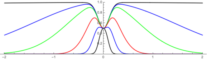
Figure 21: Pair coincidence rates versus detection time difference with synchronized Gaussian pulses and Gaussian parent beam lineshapes. The curves are the function in Equation 86 with $\mathcal{V}=0.5$ and $\delta\nu=0$ fixed and a fixed parent beam coherence time, but with different pulse widths: from uppermost to the lowest the values of the product $\sigma_{t\;pulse}\;\sigma_{\nu\;beam}$ are 10,1,0.5,0.2,0.1 and 0.05.

We can see the transition between the two limits describe above, when the pulse is very wide compared to the parent beam coherence time, and when the pulse is very narrow. For intermediate cases we can see the two-peaked shape of the pairs distribution appear, evolve, and then disappear again.

C.4.2 Extension to a regular train of separated, synchronous, symmetric pulses

In a typical experiment we would create not just a single pulse at each input but a pulse train, usually repeating identical pulses at regularly spaced intervals. We can extend the above analysis to pulse train input beams very easily, provided we satisfy the criterion that the pulses are well-separated. This requires at least these two conditions:

• Each pulse is over by the time the next one starts, e.g. at any given time only one pulse in the train can have non-negligible intensity.

• The interval $\Delta T$ between pulses is long compared to the widths of the pulses themselves.

As a rough rule of thumb in the case of Gaussians we would want $\Delta T\geq 10\,\sigma_{t\;pulse}$, which will be sure to satisfy both these conditions. If the pulses are not well-separated in the above sense then one can certainly still calculate an HOM interference effect, but we would have to consider an harmonic analysis of the pulse train function rather than examining the profile of each individual pulse.

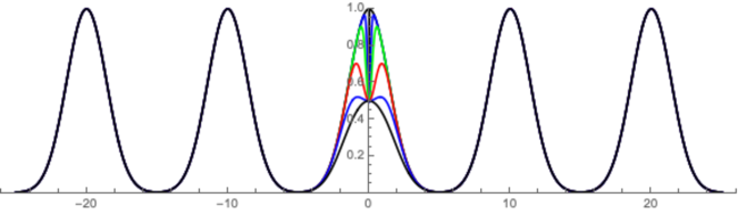
Figure 22: Pair coincidence rates versus detection time difference for a synchronized train of Gaussian pulses. The selection of curves is very similar to that in Figure 21, with $\mathcal{V}=0.5$ and $\delta\nu=0$ fixed. But now we keep the pulse length $\sigma_{t\;pulse}$ fixed, here at $1/10$ of the pulse interval, and instead vary the parent beam coherence times; as in Figure 21, from uppermost to the lowest the values used for the product $\sigma_{t\;pulse}\;\sigma_{\nu\;beam}$ are 10,1,0.5,0.2,0.1 and 0.05.

Qualitatively speaking, in the case that the pulses in the train are well-separated, as above, and the arrival of a pulse in one input channel at the beam splitter is always synchronized with a pulse in the other channel, then we can think of the experiment as simply a repetition at intervals of the single-pulse version described in Section C.4.1. The analysis of the “central” peak around $\Delta t=0$ in the pairs distribution remains exactly as in the single-pulse case. The only change in the pairs distribution is the appearance of pairs with larger $\Delta t$’s, away from $\Delta t=0$, which correspond to the arrival of photons pairs from non-synchronous pulses, e.g. from different “beats” of the two beams.

These “off-beat” pairs will, clearly, appear near times where $\Delta t$ is some integer multiple of the inter-pulse spacing $\Delta T$. Each of these groupings is essentially a copy of the classical term in Equation 86; or equivalently the result of defining the intensity envelopes $I_{a}(t)$ and $I_{b}(t)$ in the classical term of Equation 79 to contain the entire pulse train. The important point for our quickie analysis is, that in the case of well-separated pulses the “off-beat” pairs will not show any detectable effect of quantum interference: only the central pairs peak shows an effect, and that is identical to that in the single-pulse case.

With this in hand we can now write the result for a regular train of synchronized Gaussian pulses at the input channels, in the case that the pulses are well-separated. All we need to do is to copy over Equation 86 and repeat the classical term at intervals with spacing $\Delta T$:

$$\frac{dN^{(2)}}{d\,\Delta t}\;\propto\;\left[\sum_{n}G(\Delta t;n\,\Delta T,\sqrt{2}\,\sigma_{t\;pulse})\right]-\mathcal{V}\;G\left(\Delta t;0,\frac{\sqrt{2}\;\sigma_{t\;pulse}}{\sqrt{1+(4\pi\sigma_{\nu\;beam}\,\sigma_{t\;pulse}})^{2}}\right)\,\cos{(2\pi\,\delta\nu\,\Delta t)}$$ (88)

Equation C47 is now a full functional form for the pair rates in the case of a regular train of separated, synchronous Gaussian pulses, in terms of just five parameters: pulse width, pulse interval spacing, parent beam lineshape width, parent beam frequency mismatch, and HOM visibility at $\Delta t=0$. For illustration we have plotted Eq. C47 in Figure 22, where we have kept the pulse width fixed but varied the parent beam linewidth to cover the same range of cases as shown in Figure 21.

The two limiting cases are clearly visible. First, where the parent beams have a coherence time much shorter than the pulse width and we see a distinct HOM dip at $\Delta t=0$ ; secondly, where the pulse is narrow compared to the beam coherence time and the central peak of the pairs distribution is just a half-height copy of all the surrounding off-beat peaks. In between we see the evolution of the central peak shape to being distinctly two-peaked and then single-peaked again.

References

- Acín et al. (2018) A. Acín, I. Bloch, H. Buhrman, T. Calarco, C. Eichler, J. Eisert, D. Esteve, N. Gisin, S. J. Glaser, F. Jelezko, S. Kuhr, M. Lewenstein, M. F. Riedel, P. O. Schmidt, R. Thew, A. Wallraff, I. Walmsley, and F. K. Wilhelm, New Journal of Physics 20, 080201 (2018).
- Simon (2017) C. Simon, Nature Photonics 11, 678 (2017).
- Alsing et al. (2022) P. Alsing, P. Battle, J. C. Bienfang, T. Borders, T. Brower-Thomas, L. Carr, F. Chong, S. Dadras, B. DeMarco, I. Deutsch, E. Figueroa, D. Freedman, H. Everitt, D. Gauthier, E. Johnston-Halperin, J. Kim, M. Kira, P. Kumar, P. Kwiat, J. Lekki, A. Loiacono, M. Loncar, J. R. Lowell, M. Lukin, C. Merzbacher, A. Miller, C. Monroe, J. Pollanen, D. Pappas, M. Raymer, R. Reano, B. Rodenburg, M. Savage, T. Searles, and J. Ye, “Accelerating progress towards practical quantum advantage: A national science foundation project scoping workshop,” (2022).
- Lo et al. (2012) H.-K. Lo, M. Curty, and B. Qi, Physical Review Letters 108 (2012), 10.1103/physrevlett.108.130503.
- Lloyd et al. (2001) S. Lloyd, M. Shahriar, J. Shapiro, and P. Hemmer, Phys. Rev. Lett. 87, 167903 (2001).
- Kimble (2008) H. J. Kimble, Nature 453, 1023 (2008).
- Awschalom et al. (2021) D. Awschalom, K. K. Berggren, H. Bernien, S. Bhave, L. D. Carr, P. Davids, S. E. Economou, D. Englund, A. Faraon, M. Fejer, S. Guha, M. V. Gustafsson, E. Hu, L. Jiang, J. Kim, B. Korzh, P. Kumar, P. G. Kwiat, M. Lončar, M. D. Lukin, D. A. Miller, C. Monroe, S. W. Nam, P. Narang, J. S. Orcutt, M. G. Raymer, A. H. Safavi-Naeini, M. Spiropulu, K. Srinivasan, S. Sun, J. Vučković, E. Waks, R. Walsworth, A. M. Weiner, and Z. Zhang, PRX Quantum 2, 017002 (2021).
- Hensen et al. (2016) B. Hensen, N. Kalb, M. S. Blok, A. E. Dréau, A. Reiserer, R. F. L. Vermeulen, R. N. Schouten, M. Markham, D. J. Twitchen, K. Goodenough, D. Elkouss, S. Wehner, T. H. Taminiau, and R. Hanson, Scientific Reports 6, 30289 (2016).
- Valivarthi et al. (2016) R. Valivarthi, M. G. Puigibert, Q. Zhou, G. H. Aguilar, V. B. Verma, F. Marsili, M. D. Shaw, S. W. Nam, D. Oblak, and W. Tittel, Nature Photonics 10, 676 (2016).
- Sun et al. (2016) Q.-C. Sun, Y.-L. Mao, S.-J. Chen, W. Zhang, Y.-F. Jiang, Y.-B. Zhang, W.-J. Zhang, S. Miki, T. Yamashita, H. Terai, X. Jiang, T.-Y. Chen, L.-X. You, X.-F. Chen, Z. Wang, J.-Y. Fan, Q. Zhang, and J.-W. Pan, Nature Photonics 10, 671 (2016).
- Valivarthi et al. (2020) R. Valivarthi, S. I. Davis, C. Peña, S. Xie, N. Lauk, L. Narváez, J. P. Allmaras, A. D. Beyer, Y. Gim, M. Hussein, G. Iskander, H. L. Kim, B. Korzh, A. Mueller, M. Rominsky, M. Shaw, D. Tang, E. E. Wollman, C. Simon, P. Spentzouris, D. Oblak, N. Sinclair, and M. Spiropulu, PRX Quantum 1, 020317 (2020).
- Puigibert et al. (2020) M. l. G. Puigibert, M. F. Askarani, J. H. Davidson, V. B. Verma, M. D. Shaw, S. W. Nam, T. Lutz, G. C. Amaral, D. Oblak, and W. Tittel, Phys. Rev. Res. 2, 013039 (2020).
- Cao et al. (2020) M. Cao, F. Hoffet, S. Qiu, A. S. Sheremet, and J. Laurat, Optica 7, 1440 (2020).
- Slodička et al. (2013) L. Slodička, G. Hétet, N. Röck, P. Schindler, M. Hennrich, and R. Blatt, Phys. Rev. Lett. 110, 083603 (2013).
- van Leent et al. (2022) T. van Leent, M. Bock, F. Fertig, R. Garthoff, S. Eppelt, Y. Zhou, P. Malik, M. Seubert, T. Bauer, W. Rosenfeld, W. Zhang, C. Becher, and H. Weinfurter, Nature 607, 69 (2022).
- Lago-Rivera et al. (2021) D. Lago-Rivera, S. Grandi, J. V. Rakonjac, A. Seri, and H. de Riedmatten, Nature 594, 37 (2021).
- Yu et al. (2020) Y. Yu, F. Ma, X.-Y. Luo, B. Jing, P.-F. Sun, R.-Z. Fang, C.-W. Yang, H. Liu, M.-Y. Zheng, X.-P. Xie, W.-J. Zhang, L.-X. You, Z. Wang, T.-Y. Chen, Q. Zhang, X.-H. Bao, and J.-W. Pan, Nature 578, 240 (2020).
- Neumann et al. (2022) S. P. Neumann, A. Buchner, L. Bulla, M. Bohmann, and R. Ursin, Nature Communications 13, 6134 (2022).
- Xia et al. (2015) W. Xia, Y. Wen, C. H. Foh, D. Niyato, and H. Xie, IEEE Communications Surveys & Tutorials 17, 27 (2015).
- Lo Bello and Steiner (2019) L. Lo Bello and W. Steiner, Proceedings of the IEEE 107, 1094 (2019).
- Wehner et al. (2018) S. Wehner, D. Elkouss, and R. Hanson, Science 362, eaam9288 (2018), https://www.science.org/doi/pdf/10.1126/science.aam9288 .
- Pompili et al. (2022) M. Pompili, C. Delle Donne, I. te Raa, B. van der Vecht, M. Skrzypczyk, G. Ferreira, L. de Kluijver, A. J. Stolk, S. L. N. Hermans, P. Pawełczak, W. Kozlowski, R. Hanson, and S. Wehner, npj Quantum Information 8, 121 (2022).
- Fang et al. (2022) K. Fang, J. Zhao, X. Li, Y. Li, and R. Duan, “Quantum network: from theory to practice,” (2022).
- Mannalath and Pathak (2022) V. Mannalath and A. Pathak, “Multiparty entanglement routing in quantum networks,” (2022).
- Chehimi and Saad (2022) M. Chehimi and W. Saad, IEEE Network 36, 32 (2022).
- Liu et al. (2022) M. Liu, J. Allcock, K. Cai, S. Zhang, and J. C. Lui, IEEE Network 36, 56 (2022).
- Azuma et al. (2022) K. Azuma, S. E. Economou, D. Elkouss, P. Hilaire, L. Jiang, H.-K. Lo, and I. Tzitrin, “Quantum repeaters: From quantum networks to the quantum internet,” (2022).
- Cabrillo et al. (1999) C. Cabrillo, J. I. Cirac, P. Garcí a-Fernández, and P. Zoller, Physical Review A 59, 1025 (1999).
- Lipiński et al. (2011) M. Lipiński, T. Włostowski, J. Serrano, and P. Alvarez, in 2011 IEEE International Symposium on Precision Clock Synchronization for Measurement, Control and Communication (2011) pp. 25–30.
- Ronen and Lipinski (2015) O. Ronen and M. Lipinski, in 2015 IEEE International Symposium on Precision Clock Synchronization for Measurement, Control, and Communication (ISPCS) (2015) pp. 76–81.
- Dierikx et al. (2016) E. F. Dierikx, A. E. Wallin, T. Fordell, J. Myyry, P. Koponen, M. Merimaa, T. J. Pinkert, J. C. J. Koelemeij, H. Z. Peek, and R. Smets, IEEE Transactions on Ultrasonics, Ferroelectrics, and Frequency Control 63, 945 (2016).
- Xavier et al. (2008) G. B. Xavier, G. V. de Faria, G. P. T. ao, and J. P. von der Weid, Opt. Express 16, 1867 (2008).
- Kidoh et al. (1981) Y. Kidoh, Y. Suematsu, and K. Furuya, IEEE Journal of Quantum Electronics 17, 991 (1981).
- Chen et al. (2007) J. Chen, G. Wu, Y. Li, E. Wu, and H. Zeng, Opt. Express 15, 17928 (2007).
- Simmons (2014) J. Simmons, “1935-3839,” in Optical Network Design and Planning (Springer International Publishing, 2014).
- Khorsandroo et al. (2021) S. Khorsandroo, A. G. Sánchez, A. S. Tosun, J. Arco, and R. Doriguzzi-Corin, Computer Networks 192, 107981 (2021).
- Sharma et al. (2011) S. Sharma, D. Katramatos, and D. Yu (Association for Computing Machinery, New York, NY, USA, 2011).
- Katramatos et al. (2012) D. Katramatos, S. Sharma, and D. Yu, , 53–62 (2012).
- Cer (1983) Computer Networks (1976) 7, 307 (1983).
- Illiano et al. (2022) J. Illiano, M. Caleffi, A. Manzalini, and A. S. Cacciapuoti, Computer Networks 213, 109092 (2022).
- Kurose and Ross (2022) J. Kurose and K. Ross, Computer Networking: A Top-down Approach (Pearson, 2022).
- Namazi et al. (2017) M. Namazi, C. Kupchak, B. Jordaan, R. Shahrokhshahi, and E. Figueroa, Phys. Rev. Appl. 8, 034023 (2017).
- Wang et al. (2022) Y. Wang, A. N. Craddock, R. Sekelsky, M. Flament, and M. Namazi, Phys. Rev. Appl. 18, 044058 (2022).
- Kumar et al. (2023) A. Kumar, A. Suleymanzade, M. Stone, L. Taneja, A. Anferov, D. I. Schuster, and J. Simon, Nature 615, 614 (2023).
- Lipiński et al. (2018) M. Lipiński, E. van der Bij, J. Serrano, T. Włostowski, G. Daniluk, A. Wujek, M. Rizzi, and D. Lampridis, in 2018 IEEE International Symposium on Precision Clock Synchronization for Measurement, Control, and Communication (ISPCS) (2018) pp. 1–7.
- Bersin et al. (2023) E. Bersin, M. Grein, M. Sutula, R. Murphy, Y. Q. Huan, M. Stevens, A. Suleymanzade, C. Lee, R. Riedinger, D. J. Starling, P.-J. Stas, C. M. Knaut, N. Sinclair, D. R. Assumpcao, Y.-C. Wei, E. N. Knall, B. Machielse, D. D. Sukachev, D. S. Levonian, M. K. Bhaskar, M. Lončar, S. Hamilton, M. Lukin, D. Englund, and P. B. Dixon, (2023), arXiv:2307.15696 [quant-ph] .
- Bock et al. (2018) M. Bock, P. Eich, S. Kucera, M. Kreis, A. Lenhard, C. Becher, and J. Eschner, Nature Communications 9, 1998 (2018).
- van Leent et al. (2020) T. van Leent, M. Bock, R. Garthoff, K. Redeker, W. Zhang, T. Bauer, W. Rosenfeld, C. Becher, and H. Weinfurter, Phys. Rev. Lett. 124, 010510 (2020).
- Michelberger et al. (2015) P. Michelberger, T. Champion, M. Sprague, K. Kaczmarek, M. Barbieri, X. Jin, D. England, W. Kolthammer, D. Saunders, J. Nunn, et al., New J. Phys. 17, 043006 (2015).
- Peres (1996) A. Peres, Phys. Rev. Lett. 77, 1413 (1996).
- Clauser et al. (1969) J. F. Clauser, M. A. Horne, A. Shimony, and R. A. Holt, Phys. Rev. Lett. 23, 880 (1969).
- Luo et al. (2022) X.-Y. Luo, Y. Yu, J.-L. Liu, M.-Y. Zheng, C.-Y. Wang, B. Wang, J. Li, X. Jiang, X.-P. Xie, Q. Zhang, X.-H. Bao, and J.-W. Pan, Phys. Rev. Lett. 129, 050503 (2022).
- Uphoff et al. (2016) M. Uphoff, M. Brekenfeld, G. Rempe, and S. Ritter, Applied Physics B 122, 1 (2016).
- Dideriksen et al. (2021) K. B. Dideriksen, R. Schmieg, M. Zugenmaier, and E. S. Polzik, Nature communications 12, 3699 (2021).
- Gardiner and Collett (1985) C. W. Gardiner and M. J. Collett, Physical Review A 31, 3761 (1985).
- Duan et al. (2001) L.-M. Duan, M. D. Lukin, J. I. Cirac, and P. Zoller, Nature 414, 413 (2001).
- Gardiner and Zoller (2004) C. Gardiner and P. Zoller, Quantum noise: a handbook of Markovian and non-Markovian quantum stochastic methods with applications to quantum optics (Springer Science & Business Media, 2004).