N-grams Bayesian Differential Privacy

Osman Ramadan, Microsoft, osramada@microsoft.com
James Withers, Microsoft, jawithe@microsoft.com
Douglas Orr**footnotemark: *, Graphcore, douglas.orr99@gmail.com
Abstract

Differential privacy has gained popularity in machine learning as a strong privacy guarantee, in contrast to privacy mitigation techniques such as k-anonymity. However, applying differential privacy to n-gram counts significantly degrades the utility of derived language models due to their large vocabularies. We propose a differential privacy mechanism that uses public data as a prior in a Bayesian setup to provide tighter bounds on the privacy loss metric ϵitalic-ϵ\epsilon, and thus better privacy-utility trade-offs. It first transforms the counts to log space, approximating the distribution of the public and private data as Gaussian. The posterior distribution is then evaluated and softmax is applied to produce a probability distribution. This technique achieves up to 85% reduction in KL-divergence compared to previously known mechanisms at ϵitalic-ϵ\epsilon equals 0.1. We compare our mechanism to k-anonymity in a n-gram language modelling task and show that it offers competitive performance at large vocabulary sizes, while also providing superior privacy protection.

Keywords: Differential Privacy, n-grams, k-anonymity, NLP.

11footnotetext: During his time at Microsoft

1 Introduction

In today’s data-driven world, protecting the privacy of individuals’ information is of the utmost importance to data curators, both as an ethical consideration and as a legal requirement, e.g. Article 29 of the European Union’s General Data Protection Regulation describes privacy risks as singling out, linkability and inference.

Sequential data, such as DNA sequences, textual data and mobility traces, is being increasingly used in a variety of real-life applications, spanning from genome and language modeling to location-based recommendation systems. However, using such data poses considerable threats to individual privacy. It might be used by a malicious adversary to discover potential sensitive information about a data owner such as their habits, religion or relationships.

Data anonymisation is a popular means of privacy preservation in datasets. One such example is the K-anonymity framework (knon, ), (dp-any, ), which anonymises data by generalising quasi identifiers, ensuring that an individual’s data is indistinguishable from at least (k1𝑘1k-1) others’. However, even the K-anonymity approach still poses privacy concerns, since it is deterministic and susceptible to privacy attacks, such as linkage attacks. It is therefore urgent to respond to the failure of existing anonymisation techniques by developing new schemes with provable privacy guarantees.

Differential privacy is one of the only schemes that can be used to provide such guarantees. The main idea of differential privacy is to add noise to operations performed on a dataset so that an adversary cannot decide whether a particular user is included in the dataset or not. Due to the inherent sequentiality and high-dimensionality of sequential data, it is challenging to apply differential privacy. In particular, naively adding noise to the occurrence counts of each distinct sequence or n-gram in the dataset negatively impacts the utility (seq-dp, ). Other approaches rely on applying differential privacy to the operation of set union (union-set, ) by collecting a subset of items from each user, taking the union of such subsets, and disclosing the items whose noisy counts rise above a certain threshold. However, these mechanisms do not learn the counts or the probability distribution of these items, which requires adding significantly large noise. One possible direction for mitigating the curse of dimensionality is to leverage Bayesian learning, utilising public data to shape our prior of the private data (bay-dp-sample, ). Learning a Bayesian model typically involves sampling from a posterior distribution, therefore the learning process is inherently randomized.

In this paper, we model applying differential privacy as taking a sample from the posterior distribution in a Bayesian setup. We propose a practical mechanism that efficiently uses public data to improve the utility and reduce the privacy loss. The paper is organised as follows. Section 2 gives a gentle introduction to differential privacy, defining core concepts and mechanisms that achieve differential privacy. Section 3 provides a walk-through our proposed mechanism, and Section 4 discusses the experimental results of our mechanism in comparison with other mechanisms. Finally, Section 5 tries to empirically evaluate the privacy loss of our mechanism by performing membership inference attacks. Proofs of the theorems, claims and corollaries are included in the Appendices.

2 Preliminaries

In this section, we review the definition of (ϵ,δ)italic-ϵ𝛿(\epsilon,\delta)-differential privacy, and the exponential mechanisms to achieve it.

2.1 Differential Privacy

Differential privacy is a statistical guarantee of privacy protection. It renders individuals’ information indistinguishable by adding noise (dp, ), (dp2, ). Let 𝒱𝒱\mathcal{V} be the set of the attributes and 𝒰𝒰\mathcal{U} the set of users their information we want to protect, then 𝒟=(𝐜1,,𝐜|𝒰|)𝒟superscript𝐜1superscript𝐜𝒰\mathcal{D}=(\mathbf{c}^{1},...,\mathbf{c}^{|\mathcal{U}|}) is a database of counts where each row 𝚫𝐜n|𝒱|𝚫superscript𝐜𝑛superscript𝒱\mathbf{\Delta c}^{n}\in\mathbb{R}^{|\mathcal{V}|} corresponds to a user n𝒰𝑛𝒰n\in\mathcal{U} and ΔcinΔsuperscriptsubscript𝑐𝑖𝑛\Delta c_{i}^{n} is user n𝑛n count of attribute i𝒱𝑖𝒱i\in\mathcal{V}, i.e. 𝐜=n𝒰𝚫𝐜n𝐜subscript𝑛𝒰𝚫superscript𝐜𝑛\mathbf{c}=\sum_{n\in\mathcal{U}}\mathbf{\Delta c}^{n}. We refer to the attributes set 𝒱𝒱\mathcal{V}, which is independent of the users, as the vocabulary and the attributes as words, but they can equally refer to n-grams. The user adjacency is defined such that 𝒟𝒟\mathcal{D} and 𝒟nsubscript𝒟𝑛\mathcal{D}_{-n} are two adjacent datasets, in which 𝒟nsubscript𝒟𝑛\mathcal{D}_{-n} does not include user n𝑛n.

Definition 1.

(Differential Privacy) Let ϵ>0italic-ϵ0\epsilon>0 and δ0𝛿0\delta\geq 0 be given privacy parameters. We say a randomized mechanism :𝒟(𝒟):𝒟𝒟\mathcal{M}:\mathcal{D}\rightarrow\mathcal{M}(\mathcal{D}) satisfies (ϵ,δ)italic-ϵ𝛿(\epsilon,\delta)-differential privacy, if for any adjacent datasets 𝒟𝒟\mathcal{D} and 𝒟n,n𝒰subscript𝒟𝑛𝑛𝒰\mathcal{D}_{-n},\;n\in\mathcal{U} and all measurable sets 𝒮Range()𝒮𝑅𝑎𝑛𝑔𝑒\mathcal{S}\subseteq Range(\mathcal{M}), we have:

Pr[(𝒟)𝒮)]eϵPr[(𝒟n)𝒮]+δPr[\mathcal{M}(\mathcal{D})\in\mathcal{S})]\leq e^{\epsilon}Pr[\mathcal{M}(\mathcal{D}_{-n})\in\mathcal{S}]+\delta

To apply differential privacy to a function f𝑓f we need to know its sensitivity:

Definition 2.

(ljsubscript𝑙𝑗l_{j}-sensitivity) The ljsubscript𝑙𝑗l_{j}-sensitivity of a function f:𝒟f(𝒟)d:𝑓𝒟𝑓𝒟superscript𝑑f:\mathcal{D}\rightarrow f(\mathcal{D})\in\mathbb{R}^{d} is:

Δfj=maxn𝒰f(𝒟)f(𝒟n)j\left\lVert\Delta f\right\rVert_{j}=\max_{n\in\mathcal{U}}\left\lVert f(\mathcal{D})-f(\mathcal{D}_{-n})\right\rVert_{j}

2.2 The Exponential Mechanism

We define two standard exponential mechanisms that achieve differential privacy, specifically the Laplace and Gaussian mechanisms (dp, ), (dp2, ).

Definition 3.

(Laplace Mechanism) For any function f:𝒟d:𝑓𝒟superscript𝑑f:\mathcal{D}\rightarrow\mathbb{R}^{d}, the mechanism:

lap(𝒟,f,ϵ)=f(𝒟)+𝐞subscript𝑙𝑎𝑝𝒟𝑓italic-ϵ𝑓𝒟𝐞\mathcal{M}_{lap}(\mathcal{D},f,\epsilon)=f(\mathcal{D})+\mathbf{e}
eiLap(ϵΔf1)similar-tosubscript𝑒𝑖𝐿𝑎𝑝italic-ϵsubscriptdelimited-∥∥Δ𝑓1e_{i}\sim Lap(\frac{\epsilon}{\left\lVert\Delta f\right\rVert_{1}})

gives (ϵ,0)italic-ϵ0(\epsilon,0)-differential privacy, where Lap(b)𝐿𝑎𝑝𝑏Lap(b) is a b-scale Laplace distribution and Δf1subscriptdelimited-∥∥Δ𝑓1\left\lVert\Delta f\right\rVert_{1} is the l1subscript𝑙1l_{1}-sensitivity of f𝑓f.

Definition 4.

(Gaussian Mechanism) For any function f:𝒟d:𝑓𝒟superscript𝑑f:\mathcal{D}\rightarrow\mathbb{R}^{d}, the mechanism:

Gau(𝒟,f,ϵ,δ)=f(𝒟)+𝜼subscript𝐺𝑎𝑢𝒟𝑓italic-ϵ𝛿𝑓𝒟𝜼\mathcal{M}_{Gau}(\mathcal{D},f,\epsilon,\delta)=f(\mathcal{D})+\boldsymbol{\eta}
ηi𝒩(0,σ2)similar-tosubscript𝜂𝑖𝒩0superscript𝜎2\eta_{i}\sim\mathcal{N}(0,\sigma^{2})

gives (ϵ,δ)italic-ϵ𝛿(\epsilon,\delta)-differential privacy, for ϵ(0,1)italic-ϵ01\epsilon\in(0,1) and σ>2ln(1.25/δ)Δf2ϵ𝜎2𝑙𝑛1.25𝛿subscriptdelimited-∥∥Δ𝑓2italic-ϵ\sigma>\sqrt{2ln(1.25/\delta)}\frac{\left\lVert\Delta f\right\rVert_{2}}{\epsilon}.

3 Bayesian Approach to Utilise Public Data

Let 𝜶𝜶\boldsymbol{\alpha} be the public counts, defined as a one row database, and the private database 𝒟𝒟\mathcal{D} counts are defined over the public database vocabulary 𝒱𝒱\mathcal{V}. To combine public and private counts in Bayesian differential privacy settings, we model the public data as the prior and the private data as the likelihood. Then, we compute the posterior and take a sample from it as the output (privacy-free, ). In the simple case, the public counts can be modelled as a Dirichlet distribution and the private counts as a Multinomial distribution (bay-ngram, ), (bay-dp-bsc, ). However, to form a differential private mechanism we must truncate the Dirichlet distribution at the tails to prevent the sensitivity of the private counts from exploding (bay-dp-sample, ), (bay-dp-bsc, ). Instead, we can approximate the Dirichlet distribution of the public counts in the softmax space as a Gaussian distribution 𝒩(𝐡|𝝁p,σp𝐈;𝜶)𝒩conditional𝐡subscript𝝁𝑝subscript𝜎𝑝𝐈𝜶\mathcal{N}(\mathbf{h}|\boldsymbol{\mu}_{p},\sigma_{p}\mathbf{I};\boldsymbol{\alpha}) (lap-approx, ), (vae, ) where σpsubscript𝜎𝑝\sigma_{p} is the standard deviation and:

μpi=log(αi+1)1|𝒱|j|𝒱|log(αj+1)subscript𝜇𝑝𝑖subscript𝛼𝑖11𝒱superscriptsubscript𝑗𝒱subscript𝛼𝑗1\mu_{pi}=\log(\alpha_{i}+1)-\frac{1}{|\mathcal{V}|}\sum_{j}^{|\mathcal{V}|}\log(\alpha_{j}+1) (1)

which represents the prior distribution and the addition of 1 is important to avoid running into infinity. Using the private counts as a likelihood distribution in the Bayesian settings requires applying the softmax, i.e. the posterior distribution is σ(𝐡)𝒩(𝐡|𝝁p,σp𝐈)𝜎𝐡𝒩conditional𝐡subscript𝝁𝑝subscript𝜎𝑝𝐈\sigma(\mathbf{h})\mathcal{N}(\mathbf{h}|\boldsymbol{\mu}_{p},\sigma_{p}\mathbf{I}). However, this is not a closed form posterior and so a differentially-private iterative sampling algorithm is required (dp-wo-sen, ). To mitigate this problem, we use a trick by modelling the overall private counts as one sample in the softmax/log space as follows, where cisubscript𝑐𝑖c_{i} is the total counts of word i𝑖i:

x^i=log(ci+1)1|𝒱|j|𝒱|log(cj+1)subscript^𝑥𝑖subscript𝑐𝑖11𝒱superscriptsubscript𝑗𝒱subscript𝑐𝑗1\hat{x}_{i}=\log(c_{i}+1)-\frac{1}{|\mathcal{V}|}\sum_{j}^{|\mathcal{V}|}\log(c_{j}+1) (2)

The adjacent database with user n𝑛n removed is defined as:

(x^n)i=log(ciΔcin+1)1|𝒱|j|𝒱|log(cjΔcjn+1)subscriptsubscript^𝑥𝑛𝑖subscript𝑐𝑖Δsubscriptsuperscript𝑐𝑛𝑖11𝒱superscriptsubscript𝑗𝒱subscript𝑐𝑗Δsubscriptsuperscript𝑐𝑛𝑗1(\hat{x}_{-n})_{i}=\log(c_{i}-\Delta c^{n}_{i}+1)-\frac{1}{|\mathcal{V}|}\sum_{j}^{|\mathcal{V}|}\log(c_{j}-\Delta c^{n}_{j}+1) (3)

Consequently, the likelihood can be represented by a Gaussian distribution: 𝒩(𝐱|𝐡,σl𝐈)𝒩conditional𝐱𝐡subscript𝜎𝑙𝐈\mathcal{N}(\mathbf{x}|\mathbf{h},\sigma_{l}\mathbf{I}), where σlsubscript𝜎𝑙\sigma_{l} does not depend on the private database. Since a Gaussian is a conjugate prior to itself, the posterior is also a Gaussian distribution: 𝒩(𝐡|𝝁ps,σps𝐈;𝝁p,𝒙^,σp,σl)𝒩conditional𝐡subscript𝝁𝑝𝑠subscript𝜎𝑝𝑠𝐈subscript𝝁𝑝bold-^𝒙subscript𝜎𝑝subscript𝜎𝑙\mathcal{N}(\mathbf{h}|\boldsymbol{\mu}_{ps},\sigma_{ps}\mathbf{I};\boldsymbol{\mu}_{p},\boldsymbol{\hat{x}},\sigma_{p},\sigma_{l}), where 𝝁ps=ρ𝒙^+(1ρ)𝝁psubscript𝝁𝑝𝑠𝜌bold-^𝒙1𝜌subscript𝝁𝑝\boldsymbol{\mu}_{ps}=\rho\boldsymbol{\hat{x}}+(1-\rho)\boldsymbol{\mu}_{p}, σps=ρσpsubscript𝜎𝑝𝑠𝜌subscript𝜎𝑝\sigma_{ps}=\rho\sigma_{p} and ρ=σlσl+σp𝜌subscript𝜎𝑙subscript𝜎𝑙subscript𝜎𝑝\rho=\frac{\sigma_{l}}{\sigma_{l}+\sigma_{p}} is a hyperparameter to be chosen. We then apply the softmax to get the normalised probability distribution:

θi=softmax(𝐡)i=ehij|𝒱|ehjsubscript𝜃𝑖𝑠𝑜𝑓𝑡𝑚𝑎𝑥subscript𝐡𝑖superscript𝑒subscript𝑖superscriptsubscript𝑗𝒱superscript𝑒subscript𝑗\theta_{i}=softmax(\mathbf{h})_{i}=\frac{e^{h_{i}}}{\sum_{j}^{|\mathcal{V}|}e^{h_{j}}} (4)
Theorem 1.

Given the Gaussian mechanism \mathcal{M}:= 𝒩(𝐡|ρ𝐱^+(1ρ)𝛍p,σps𝐈)𝒩conditional𝐡𝜌bold-^𝐱1𝜌subscript𝛍𝑝subscript𝜎𝑝𝑠𝐈\mathcal{N}(\mathbf{h}|\rho\boldsymbol{\hat{x}}+(1-\rho)\boldsymbol{\mu}_{p},\sigma_{ps}\mathbf{I}) and its l2subscript𝑙2l_{2}-sensitivity:
Δ𝐱^2=𝐱^𝐱^n2ϵσpsρ2log(1.25δ)n𝒰subscriptdelimited-∥∥Δbold-^𝐱2subscriptdelimited-∥∥bold-^𝐱subscriptbold-^𝐱𝑛2italic-ϵsubscript𝜎𝑝𝑠𝜌21.25𝛿for-all𝑛𝒰\left\lVert\Delta\boldsymbol{\hat{x}}\right\rVert_{2}=\left\lVert\boldsymbol{\hat{x}}-\boldsymbol{\hat{x}}_{-n}\right\rVert_{2}\leq\frac{\epsilon\sigma_{ps}}{\rho\sqrt{2\log(\frac{1.25}{\delta})}}\>\forall n\in\mathcal{U}, then mechanism \mathcal{M} is (ϵ,δitalic-ϵ𝛿\epsilon,\delta)-differentially private, where 𝛍psubscript𝛍𝑝\boldsymbol{\mu}_{p}, 𝐱^bold-^𝐱\boldsymbol{\hat{x}} and 𝐱^nsubscriptbold-^𝐱𝑛\boldsymbol{\hat{x}}_{-n} are defined by equations 1, 2 and 3 respectively.

3.1 Word-wise Adaptive Clipping Strategy (adaclip, )

We examine the l2subscript𝑙2l_{2}-sensitivity Δ𝒙^Δbold-^𝒙\Delta\boldsymbol{\hat{x}} in Theorem 1:

Δ𝒙^22=i|𝒱|(log(1Δcin1+ci)1|𝒱|i|𝒱|log(1Δcjn1+cj))2superscriptsubscriptdelimited-∥∥Δbold-^𝒙22superscriptsubscript𝑖𝒱superscript1Δsubscriptsuperscript𝑐𝑛𝑖1subscript𝑐𝑖1𝒱superscriptsubscript𝑖𝒱1Δsubscriptsuperscript𝑐𝑛𝑗1subscript𝑐𝑗2\left\lVert\Delta\boldsymbol{\hat{x}}\right\rVert_{2}^{2}=\sum_{i}^{|\mathcal{V}|}\bigg{(}\log(1-\frac{\Delta c^{n}_{i}}{1+c_{i}})-\frac{1}{|\mathcal{V}|}\sum_{i}^{|\mathcal{V}|}\log(1-\frac{\Delta c^{n}_{j}}{1+c_{j}})\bigg{)}^{2}

We observe from the equation above that the sensitivity depends mostly on words with large user percentage contribution (Δcin1+ciΔsubscriptsuperscript𝑐𝑛𝑖1subscript𝑐𝑖\frac{\Delta c^{n}_{i}}{1+c_{i}}). That means frequent words have little effect on the sensitivity as opposed to rare words, even though they contribute the most to the utility, e.g. KL divergence. To mitigate the effect of rare words, we define a decay function w(Ni)[0,1]𝑤subscript𝑁𝑖01w(N_{i})\in[0,1] where Nisubscript𝑁𝑖N_{i} is the number of users that have the word i𝑖i in their counts. A good decay function will penalise rare words more as fewer users contributed these words and so their sensitivity effect is large. The probability mass of these rare words can be taken from the public distribution. We experimented with clamped logarithmic, exponential and linear decay functions, and they all behaved similarly, therefore we decided to pick the linear function as it is the simplest and has a constant gradient:

𝐰i=min(1,SNiC),i𝒱formulae-sequencesubscript𝐰𝑖𝑚𝑖𝑛1𝑆subscript𝑁𝑖𝐶for-all𝑖𝒱\mathbf{w}_{i}=min\big{(}1,\frac{SN_{i}}{C}\big{)},\forall i\in\mathcal{V} (5)

Where C𝐶C is the maximum per-user word count and S𝑆S is a weighting hyperparameter.

Corollary 1.

Let 𝛍ps=ρ𝐰𝐱^+(1ρ)𝛍psubscript𝛍𝑝𝑠direct-product𝜌𝐰bold-^𝐱1𝜌subscript𝛍𝑝\boldsymbol{\mu}_{ps}=\rho\mathbf{w}\odot\boldsymbol{\hat{x}}+(1-\rho)\boldsymbol{\mu}_{p} then the
modified Gaussian mechanism \mathcal{M}:= 𝒩(𝐡|𝛍ps,σps𝐈)𝒩conditional𝐡subscript𝛍𝑝𝑠subscript𝜎𝑝𝑠𝐈\mathcal{N}(\mathbf{h}|\boldsymbol{\mu}_{ps},\sigma_{ps}\mathbf{I}) is (ϵ,δitalic-ϵ𝛿\epsilon,\delta)-differentially private if Δ𝛍ps2=𝐰𝚫𝐱^+SC𝟙(𝐍CS)𝐱^n2ϵσpsρ2log(1.25δ)n𝒰subscriptdelimited-∥∥Δsubscript𝛍𝑝𝑠2subscriptdelimited-∥∥direct-product𝐰𝚫^𝐱direct-product𝑆𝐶1𝐍𝐶𝑆subscript^𝐱𝑛2italic-ϵsubscript𝜎𝑝𝑠𝜌21.25𝛿for-all𝑛𝒰\left\lVert\Delta\boldsymbol{\mu}_{ps}\right\rVert_{2}=\left\lVert\mathbf{w}\odot\mathbf{\Delta\hat{x}}+\frac{S}{C}\mathbbm{1}\Big{(}\mathbf{N}\leq\frac{C}{S}\Big{)}\odot\mathbf{\hat{x}}_{-n}\right\rVert_{2}\leq\frac{\epsilon\sigma_{ps}}{\rho\sqrt{2\log(\frac{1.25}{\delta})}}\\ \forall n\in\mathcal{U} where 𝟙1\mathbbm{1} is the indicator function, direct-product\odot is element-wise multiplication and 𝐰,S𝐰𝑆\mathbf{w},S and C𝐶C are defined in equation 5.

The l2subscript𝑙2l_{2}-sensitivity can be computed by a brute-force method that is O(W.|U|)~{}O(W.|U|), where W𝑊W is the maximum number of words each user can contribute and |𝒰|𝒰|\mathcal{U}| is the number of users in the private database. The l2subscript𝑙2l_{2}-sensitivity can also be bounded provided C𝐶C, S𝑆S and the private counts 𝐱^^𝐱\mathbf{\hat{x}}.

Claim 1.

Given S𝑆S, C𝐶C, 𝐱^^𝐱\mathbf{\hat{x}} and the number of users for each word 𝐍𝐍\mathbf{N}, then the sensitivity defined in corollary 1 is bounded as follows:

Δ𝝁ps2<𝐰𝐋C+SC|𝐱^|𝟙(𝐍CS)2n𝒰subscriptdelimited-∥∥Δsubscript𝝁𝑝𝑠2subscriptdelimited-∥∥direct-product𝐰𝐋𝐶direct-product𝑆𝐶^𝐱1𝐍𝐶𝑆2for-all𝑛𝒰\left\lVert\Delta\boldsymbol{\mu}_{ps}\right\rVert_{2}<\left\lVert\mathbf{w}\odot\mathbf{L}C+\frac{S}{C}|\mathbf{\hat{x}}|\odot\mathbbm{1}\Big{(}\mathbf{N}\leq\frac{C}{S}\Big{)}\right\rVert_{2}\forall n\in\mathcal{U}
𝐋i=(11|𝒱|)1Ni+ji|𝒱|1|𝒱|Njsubscript𝐋𝑖11𝒱1subscript𝑁𝑖superscriptsubscript𝑗𝑖𝒱1𝒱subscript𝑁𝑗\mathbf{L}_{i}=(1-\frac{1}{|\mathcal{V}|})\frac{1}{N_{i}}+\sum_{j\neq i}^{|\mathcal{V}|}\frac{1}{|\mathcal{V}|N_{j}}

Input :

{𝚫𝐜n}1|𝒰|superscriptsubscript𝚫superscript𝐜𝑛1𝒰\{\mathbf{\Delta c}^{n}\}_{1}^{|\mathcal{U}|}, 𝜶𝜶\boldsymbol{\alpha}, ϵitalic-ϵ\epsilon, δ𝛿\delta, S𝑆S, C𝐶C, ρ𝜌\rho, |𝒱|𝒱|\mathcal{V}|

Result: normalised counts 𝜽𝜽\boldsymbol{\theta}

for n1𝑛1n\leftarrow 1 to |𝒰|𝒰|\mathcal{U}| do

       𝚫𝐜nmin(C,𝚫𝐜n)𝚫superscript𝐜𝑛𝐶𝚫superscript𝐜𝑛\mathbf{\Delta c}^{n}\leftarrow\min(C,\mathbf{\Delta c}^{n}); // clamp counts to C
end for
𝐜n𝒰𝚫𝐜n𝐜subscript𝑛𝒰𝚫superscript𝐜𝑛\mathbf{c}\leftarrow\sum_{n\in\mathcal{U}}\mathbf{\Delta c}^{n}; // overall word counts 𝐍𝐍absent\mathbf{N}\leftarrow no_users_per_word({𝚫𝐜n}1|𝒰|)superscriptsubscript𝚫superscript𝐜𝑛1𝒰(\{\mathbf{\Delta c}^{n}\}_{1}^{|\mathcal{U}|}); 𝐱^log(𝐜+1)1|𝒱|log(𝐜+1)1^𝐱𝐜11𝒱subscriptdelimited-∥∥𝐜11\mathbf{\hat{x}}\leftarrow\log(\mathbf{c}+1)-\frac{1}{|\mathcal{V}|}\left\lVert\log(\mathbf{c}+1)\right\rVert_{1}; // equation 2 𝐰min(1,S𝐍C)𝐰1𝑆𝐍𝐶\mathbf{w}\leftarrow\min(1,\frac{S\mathbf{N}}{C}); // equation 5 𝐫𝐰𝐱^𝐫direct-product𝐰^𝐱\mathbf{r}\leftarrow\mathbf{w}\odot\mathbf{\hat{x}}if Using the brute-force method to estimate sensitivity then
       γ0𝛾0\gamma\leftarrow 0; // initial sensitivity for n1𝑛1n\leftarrow 1 to |𝒰|𝒰|\mathcal{U}| do
             γmax[γ,𝐰Δ𝒙^+SC𝟙(𝚫𝐜n>0)𝒙^n2]𝛾𝛾subscriptdelimited-∥∥direct-product𝐰Δbold-^𝒙𝑆𝐶1𝚫superscript𝐜𝑛0subscriptbold-^𝒙𝑛2\gamma\leftarrow\max\Big{[}\gamma,\left\lVert\mathbf{w}\odot\Delta\boldsymbol{\hat{x}}+\frac{S}{C}\mathbbm{1}(\mathbf{\Delta c}^{n}>0)\boldsymbol{\hat{x}}_{-n}\right\rVert_{2}\Big{]}
       end for
      
else
       Compute worst-case estimate of the sensitivity (γ𝛾\gamma); // claim 1
end if
σpsργ2log(1.25δ)ϵsubscript𝜎𝑝𝑠𝜌𝛾21.25𝛿italic-ϵ\sigma_{ps}\leftarrow\frac{\rho\gamma\sqrt{2\log(\frac{1.25}{\delta})}}{\epsilon}; // corollary 1 𝝁plog(𝜶+1)1|𝒱|log(𝜶+1)1subscript𝝁𝑝𝜶11𝒱subscriptdelimited-∥∥𝜶11\boldsymbol{\mu}_{p}\leftarrow\log(\boldsymbol{\alpha}+1)-\frac{1}{|\mathcal{V}|}\left\lVert\log(\boldsymbol{\alpha}+1)\right\rVert_{1}; // equation 1 𝝁psρ𝒙^+(1ρ)𝝁psubscript𝝁𝑝𝑠𝜌bold-^𝒙1𝜌subscript𝝁𝑝\boldsymbol{\mu}_{ps}\leftarrow\rho\boldsymbol{\hat{x}}+(1-\rho)\boldsymbol{\mu}_{p}  Sample 𝐡𝒩(𝐡;𝝁ps,σps𝐈)similar-to𝐡𝒩𝐡subscript𝝁𝑝𝑠subscript𝜎𝑝𝑠𝐈\mathbf{h}\sim\mathcal{N}(\mathbf{h};\boldsymbol{\mu}_{ps},\sigma_{ps}\mathbf{I})𝜽softmax(𝐡)𝜽𝑠𝑜𝑓𝑡𝑚𝑎𝑥𝐡\boldsymbol{\theta}\leftarrow softmax(\mathbf{h})
Algorithm 1 BayesianDP

3.2 Differentially Private Hyperparameter Tuning

S𝑆S, C𝐶C and ρ𝜌\rho are hyperparameters and their values directly affect the ratio between the public and private counts and the variance of the posterior distribution for a given privacy parameters (ϵ,δitalic-ϵ𝛿\epsilon,\delta). If we ignore the noise we can compare the mean output of \mathcal{M} after applying the softmax, i.e softmax(ρ𝐰𝒙^+(1ρ)𝝁p)𝑠𝑜𝑓𝑡𝑚𝑎𝑥direct-product𝜌𝐰bold-^𝒙1𝜌subscript𝝁𝑝softmax(\rho\mathbf{w}\odot\boldsymbol{\hat{x}}+(1-\rho)\boldsymbol{\mu}_{p}), to the normalised private counts distribution softmax(𝒙^)𝑠𝑜𝑓𝑡𝑚𝑎𝑥bold-^𝒙softmax(\boldsymbol{\hat{x}}) using KL-divergence. In other words, KL-divergence, for given private and public counts, is a function of S𝑆S, C𝐶C and ρ𝜌\rho. Consequently, there are optimal values S=S,C=C,ρ=ρformulae-sequence𝑆superscript𝑆formulae-sequence𝐶superscript𝐶𝜌superscript𝜌S=S^{*},C=C^{*},\rho=\rho^{*} at which the KL-divergence is minimised for any given public and private databases. ρ𝜌\rho is the weighting between private and public counts and S𝑆S and C𝐶C affect the amount of probability mass redistributed from frequent to rare words. A very small S𝑆S or very large C𝐶C transform the private counts to a uniform distribution. However, early experiments showed that C𝐶C has little effect on the KL-divergence unless the number of users is very large and/or there are rare words with high per-user counts, the latter is a clear privacy violation, so we do not vary C𝐶C and fix it to either 1 or 10 in all our experiments. Consequently, we only have two hyperparameters S,ρ𝑆𝜌S,\rho to vary and a grid-search hyperparameter tuning approach can be used at an extra cost of a small privacy budget (since we are only adding noise to scalar value) using a variant of the noisy max algorithm (private-selection, ), (private-selection2, ).

The idea of private hyperparameter tuning is to split the private counts into two non-overlapping sets, evaluate the KL-divergence between the normalised counts (𝐜𝐜1𝐜subscriptdelimited-∥∥𝐜1\frac{\mathbf{c}}{\left\lVert\mathbf{c}\right\rVert_{1}}) of the second set and the mean (𝝁pssubscript𝝁𝑝𝑠\boldsymbol{\mu}_{ps}) of the Gaussian mechanism applied to the first set for different hyperparameters values (S,ρ𝑆𝜌S,\rho). Then, add Laplace noise with privacy loss ϵ2subscriptitalic-ϵ2\epsilon_{2} to each KL-divergence score and find the hyperparameter values (S,ρsuperscript𝑆superscript𝜌S^{*},\rho^{*}) that give the minimum noisy score. Finally, using the mean (𝝁pssuperscriptsubscript𝝁𝑝𝑠\boldsymbol{\mu}_{ps}^{*}) at these values, we sample from the (ϵ,δitalic-ϵ𝛿\epsilon,\delta)-DP Gaussian mechanism and report the final privacy parameters (ϵ+ϵ2,δitalic-ϵsubscriptitalic-ϵ2𝛿\epsilon+\epsilon_{2},\delta) using the strong composition theorem (dp, ). However, estimating the sensitivity of KL-divergence can be very complex and it is easier to use the un-normalised cross-entropy since they both exhibit their global minimum at the same hyperparameter values:

q(𝐜,𝝁ps)=i|𝒱|ci(μpsilogj|𝒱|expμpsj)𝑞𝐜subscript𝝁𝑝𝑠superscriptsubscript𝑖𝒱subscript𝑐𝑖subscript𝜇𝑝𝑠𝑖superscriptsubscript𝑗𝒱subscript𝜇𝑝𝑠𝑗q(\mathbf{c},\boldsymbol{\mu}_{ps})=-\sum_{i}^{|\mathcal{V}|}c_{i}\big{(}\mu_{psi}-\log\sum_{j}^{|\mathcal{V}|}\exp{\mu_{psj}}\big{)} (6)
Theorem 2.

Given two non-overlapping sets of private counts, let 𝐜𝐜\mathbf{c} be the counts of the first set and {𝛍ps}k=1Ksuperscriptsubscriptsubscript𝛍𝑝𝑠𝑘1𝐾\{\boldsymbol{\mu}_{ps}\}_{k=1}^{K} be K𝐾K evaluations of the mean of the Gaussian mechanism in Corollary 1, applied to the second set, for different hyperparameter values (Sk,ρk)subscript𝑆𝑘subscript𝜌𝑘(S_{k},\rho_{k}). Then for any l𝑙l-Lipschitz continuous scoring function: qk=q(𝐜,𝛍ps(k))kKsubscript𝑞𝑘𝑞𝐜superscriptsubscript𝛍𝑝𝑠𝑘for-all𝑘𝐾q_{k}=q(\mathbf{c},\boldsymbol{\mu}_{ps}^{(k)})\>\forall k\in K, the mechanism: k=argminkK(qk+eLap(ϵ2|Δq|))superscript𝑘𝑎𝑟𝑔𝑚𝑖subscript𝑛𝑘𝐾similar-tosubscript𝑞𝑘𝑒𝐿𝑎𝑝italic-ϵ2Δ𝑞k^{*}=argmin_{k\in K}\big{(}q_{k}+e\sim Lap(\frac{\epsilon}{2|\Delta q|})\big{)}, is ϵitalic-ϵ\epsilon-differential private, where Lap(b)𝐿𝑎𝑝𝑏Lap(b) is a b𝑏b-scale Laplace distribution and |Δq|Δ𝑞|\Delta q| is the maximum of the scoring function sensitivities with respect to each set separately, i.e |Δq|=Δ𝑞absent|\Delta q|= max[|q(𝐜,𝛍ps)q(𝐜n,𝛍ps)|,|q(𝐜,𝛍ps)q(𝐜,𝛍𝐩𝐬n)|]𝑞𝐜subscript𝛍𝑝𝑠𝑞subscript𝐜𝑛subscript𝛍𝑝𝑠𝑞𝐜subscript𝛍𝑝𝑠𝑞𝐜subscriptsubscript𝛍𝐩𝐬𝑛\max\Big{[}\big{|}q(\mathbf{c},\boldsymbol{\mu}_{ps})-q(\mathbf{c}_{-n},\boldsymbol{\mu}_{ps})\big{|},\big{|}q(\mathbf{c},\boldsymbol{\mu}_{ps})-q(\mathbf{c},\boldsymbol{\mu_{ps}}_{-n})\big{|}\Big{]}

As mentioned before, using un-normalised cross-entropy as a scoring function instead of KL-divergence simplifies the sensitivity analysis while achieving the same result.

Claim 2.

If the scoring function in Theorem 2 is defined by Equation 6, then sensitivity |Δq|Δ𝑞|\Delta q| is bounded as follows:
|Δq|Δ𝑞absent|\Delta q|\leq
max[ρ𝐜2Δ𝛍ps2,maxn𝒰1(i|𝒱|Δcin(μpsilogj|𝒱|expμpsj))]𝜌subscriptdelimited-∥∥𝐜2subscriptdelimited-∥∥Δsubscript𝛍𝑝𝑠2subscript𝑛subscript𝒰1superscriptsubscript𝑖𝒱Δsuperscriptsubscript𝑐𝑖𝑛subscript𝜇𝑝𝑠𝑖superscriptsubscript𝑗𝒱subscript𝜇𝑝𝑠𝑗\max\bigg{[}\rho\left\lVert\mathbf{c}\right\rVert_{2}\left\lVert\Delta\boldsymbol{\mu}_{ps}\right\rVert_{2},\max_{n\in\mathcal{U}_{1}}\bigg{(}\sum_{i}^{|\mathcal{V}|}\Delta c_{i}^{n}\Big{(}\mu_{psi}-\log\sum_{j}^{|\mathcal{V}|}\exp{\mu_{psj}}\Big{)}\bigg{)}\bigg{]} <max[ρ𝐜2Δ𝛍ps2,C1i|𝒱||μpsilogj|𝒱|expμpsj|]absent𝜌subscriptdelimited-∥∥𝐜2subscriptdelimited-∥∥Δsubscript𝛍𝑝𝑠2subscript𝐶1superscriptsubscript𝑖𝒱subscript𝜇𝑝𝑠𝑖superscriptsubscript𝑗𝒱subscript𝜇𝑝𝑠𝑗<\max\bigg{[}\rho\left\lVert\mathbf{c}\right\rVert_{2}\left\lVert\Delta\boldsymbol{\mu}_{ps}\right\rVert_{2},C_{1}\sum_{i}^{|\mathcal{V}|}\Big{|}\mu_{psi}-\log\sum_{j}^{|\mathcal{V}|}\exp{\mu_{psj}}\Big{|}\bigg{]} where 𝒰1subscript𝒰1\mathcal{U}_{1} is the first private set and C1subscript𝐶1C_{1} is their maximum word count.

The bounds in Claim 2 allow us to reuse the estimated sensitivity of the second private set Δ𝝁ps2subscriptdelimited-∥∥Δsubscript𝝁𝑝𝑠2\left\lVert\Delta\boldsymbol{\mu}_{ps}\right\rVert_{2} when sampling from (ϵ,δitalic-ϵ𝛿\epsilon,\delta)-differentially private Gaussian mechanism.

Input :

{𝚫𝐜1n}1|𝒰1|superscriptsubscript𝚫superscriptsubscript𝐜1𝑛1subscript𝒰1\{\mathbf{\Delta c}_{1}^{n}\}_{1}^{|\mathcal{U}_{1}|}, {𝚫𝐜2n}1|𝒰2|superscriptsubscript𝚫superscriptsubscript𝐜2𝑛1subscript𝒰2\{\mathbf{\Delta c}_{2}^{n}\}_{1}^{|\mathcal{U}_{2}|}, 𝜶𝜶\boldsymbol{\alpha}, ϵ1subscriptitalic-ϵ1\epsilon_{1}, ϵ2subscriptitalic-ϵ2\epsilon_{2}, δ𝛿\delta, {Sk,ρk}1Ksuperscriptsubscriptsubscript𝑆𝑘subscript𝜌𝑘1𝐾\{S_{k},\rho_{k}\}_{1}^{K}, C𝐶C, |𝒱|𝒱|\mathcal{V}|

Result: normalised counts 𝜽,ϵ1+ϵ2,δ𝜽subscriptitalic-ϵ1subscriptitalic-ϵ2𝛿\boldsymbol{\theta},\epsilon_{1}+\epsilon_{2},\delta

Clamp the counts and compute 𝐜𝟏,𝐍𝟐,𝝁p,𝐱^𝟐subscript𝐜1subscript𝐍2subscript𝝁𝑝subscript^𝐱2\mathbf{c_{1}},\mathbf{N_{2}},\boldsymbol{\mu}_{p},\mathbf{\hat{x}_{2}} // Extracted from algorithm 1

for k1𝑘1k\leftarrow 1 to K𝐾K do

       𝝁psk,σpsksubscript𝝁𝑝𝑠𝑘subscript𝜎𝑝𝑠𝑘absent\boldsymbol{\mu}_{psk},\sigma_{psk}\leftarrow BayesianDP(𝐱^𝟐,𝝁p,𝐍𝟐,Sk,ρk,C,ϵ2,δsubscript^𝐱2subscript𝝁𝑝subscript𝐍2subscript𝑆𝑘subscript𝜌𝑘𝐶subscriptitalic-ϵ2𝛿\mathbf{\hat{x}_{2}},\boldsymbol{\mu}_{p},\mathbf{N_{2}},S_{k},\rho_{k},C,\epsilon_{2},\delta)qkq(𝐜𝟏,𝝁psk)+eLap(ϵ12|Δq|)subscript𝑞𝑘𝑞subscript𝐜1subscript𝝁𝑝𝑠𝑘𝑒similar-to𝐿𝑎𝑝subscriptitalic-ϵ12Δ𝑞q_{k}\leftarrow q(\mathbf{c_{1}},\boldsymbol{\mu}_{psk})+e\sim Lap(\frac{\epsilon_{1}}{2|\Delta q|}); // q𝑞q from equation 6 and |Δq|Δ𝑞|\Delta q| from claim 2
end for
iargminkK(qk)𝑖𝑎𝑟𝑔𝑚𝑖subscript𝑛𝑘𝐾subscript𝑞𝑘i\leftarrow argmin_{k\in K}(q_{k})  Sample 𝐡𝒩(𝐡;𝝁psi,σpsi𝐈)similar-to𝐡𝒩𝐡subscript𝝁𝑝𝑠𝑖subscript𝜎𝑝𝑠𝑖𝐈\mathbf{h}\sim\mathcal{N}(\mathbf{h};\boldsymbol{\mu}_{psi},\sigma_{psi}\mathbf{I})𝜽softmax(𝐡)𝜽𝑠𝑜𝑓𝑡𝑚𝑎𝑥𝐡\boldsymbol{\theta}\leftarrow softmax(\mathbf{h})
Algorithm 2 EndToEndDP

4 Experiments and Results

4.1 Dataset

For all experiments we used the Reddit data, which consists of 4.4M users, as the private dataset and the Google Billion Word (billion-word, ) as the public dataset. We extracted trigrams and their counts from these datasets to form our database. Accordingly, the vocabulary 𝒱𝒱\mathcal{V} is the total number of distinct trigrams, which is determined only by the public dataset, and the output distribution of our mechanism is the joint trigram distribution or P(w1,w2,w3)𝑃subscript𝑤1subscript𝑤2subscript𝑤3P(w_{1},w_{2},w_{3}).

4.2 Baselines

We used two simple baselines in our experiments:

  1. 1.

    The standard Laplace mechanism (dp, ), (dp2, ), where we allow each user to contribute up to W𝑊W counts overall, and add Laplace noise with scale b=W/ϵ𝑏𝑊italic-ϵb=W/\epsilon, then threshold at 0 and normalise to get a valid probability distribution.

  2. 2.

    The other baseline is a modified Laplace mechanism that utilises public counts. We first normalise the public count, then for each user independently, we normalise the user counts and subtract the normalised public counts from it. After that, we get the weighted average of the subtracted output over all the users and add Laplace noise to it. Finally we add the normalised public counts, threshold at 0 and re-normalise. In other words, the un-normalised output of the modified Laplace mechanism:

    max[n𝒰[wn(𝚫𝐜~n𝜶~)]+e+𝜶~,𝟎]subscript𝑛𝒰delimited-[]subscript𝑤𝑛𝚫superscript~𝐜𝑛bold-~𝜶𝑒bold-~𝜶0\max\Big{[}\sum_{n\in\mathcal{U}}{\big{[}w_{n}(\mathbf{\Delta\tilde{c}}^{n}-\boldsymbol{\tilde{\alpha}})\big{]}}+e+\boldsymbol{\tilde{\alpha}},\mathbf{0}\Big{]}

    Where 𝜶~bold-~𝜶\boldsymbol{\tilde{\alpha}} is the normalised public counts, 𝚫𝐜~n𝚫superscript~𝐜𝑛\mathbf{\Delta\tilde{c}}^{n} and wn=Δ𝐜n𝐜subscript𝑤𝑛Δsuperscript𝐜𝑛𝐜w_{n}=\frac{\Delta\mathbf{c}^{n}}{\mathbf{c}} are the normalised counts and weighting of user n𝑛n and eLap(ϵΔf1)similar-to𝑒𝐿𝑎𝑝italic-ϵsubscriptdelimited-∥∥Δ𝑓1e\sim Lap(\frac{\epsilon}{\left\lVert\Delta f\right\rVert_{1}}) is the Laplace noise and Δf1subscriptdelimited-∥∥Δ𝑓1\left\lVert\Delta f\right\rVert_{1} is the l1subscript𝑙1l_{1}-sensitivity of the modified mechanism.

4.3 Experimentation setup

For all experiments, the allowed word counts per user C𝐶C is set to 1 if the number of users is less than 1M, otherwise C=10𝐶10C=10. We also limit the total number of counts for each user to |𝒰|/1000𝒰1000|\mathcal{U}|/1000. These values were chosen empirically from early experiments to be good utility-privacy trade-offs. For our Bayesian mechanism, we used the brute-force method to compute the sensitivity as it gives tighter bounds. In hyperparameter tuning, we split the private data into 90%percent9090\% train set and 10%percent1010\% validation set, where we spend 2ϵ32italic-ϵ3\frac{2\epsilon}{3} on training and ϵ3italic-ϵ3\frac{\epsilon}{3} on private hyperparameter tuning, and S[103,104]𝑆superscript103superscript104S\in[10^{-3},10^{4}].

4.4 Performance under different settings

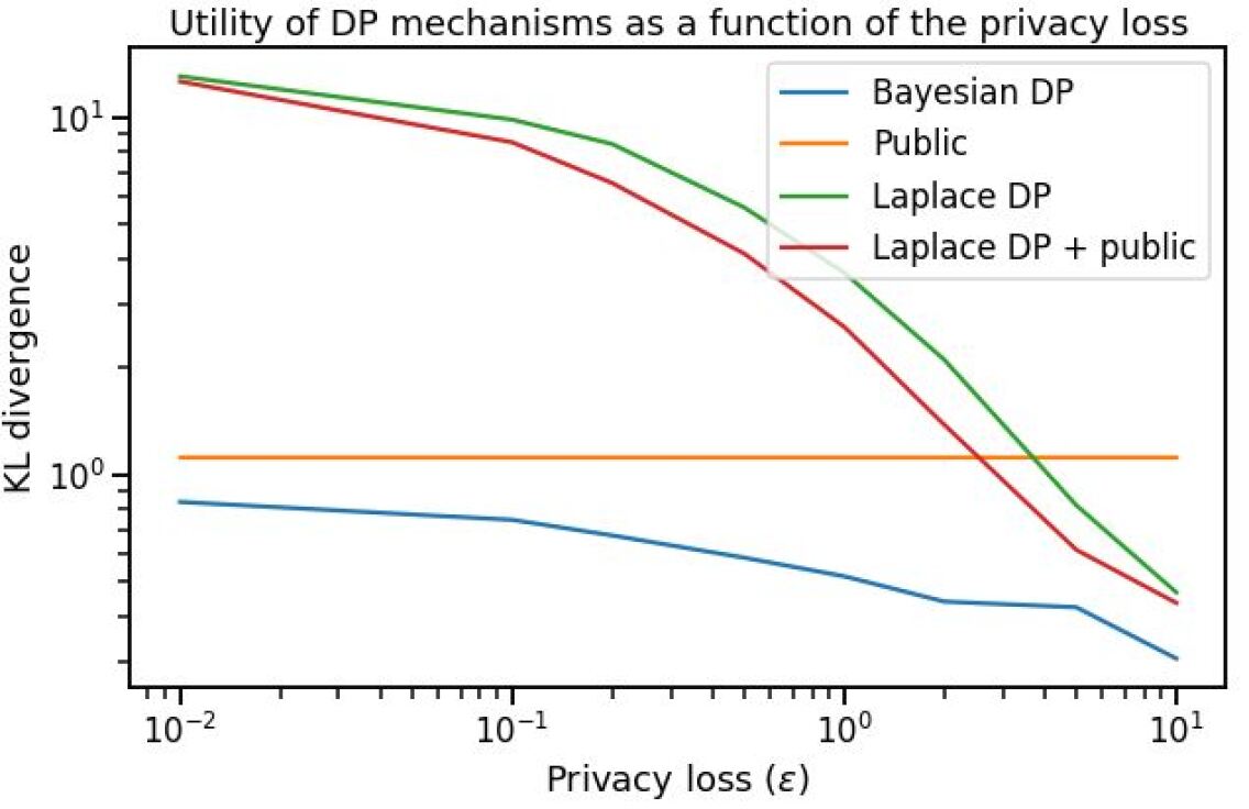
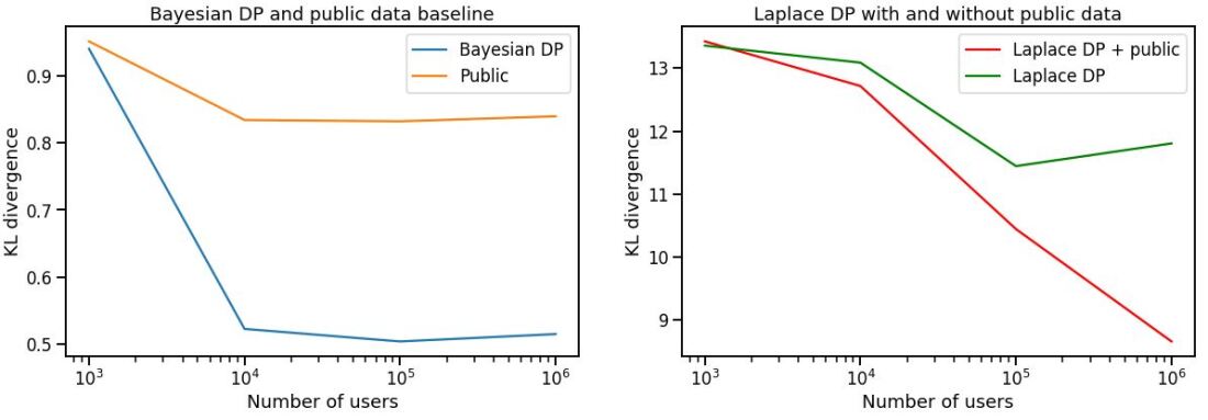
We evaluate the utility of our mechanism, measured as the KL-divergence from the private data distribution, under different settings such as the number of users in private database, the size of vocabulary set and the quality of the public data. We also compare its utility with other baseline mechanisms, as shown in Figures 1 to 4.
Refer to caption
Figure 1: KL-divergence from the private distribution vs ϵitalic-ϵ\epsilon for different mechanisms. The number of users is 4M and vocabulary size is 50K.

Refer to caption

Figure 2: Left: KL-divergence from the private distribution vs the number of users for Bayesian differential privacy compared to a public baseline. Right: Laplace differential privacy with and without public data. ϵ=0.1italic-ϵ0.1\epsilon=0.1 and vocabulary size is 50K.
Refer to caption
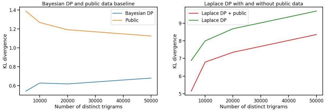
Figure 3: Left: KL-divergence from the private distribution vs the number of distinct trigrams (vocabulary size) for Bayesian differential privacy compared to a public baseline. Right: Laplace differential privacy with and without public data. The number of users is 4M and ϵ=0.1italic-ϵ0.1\epsilon=0.1.
Refer to caption
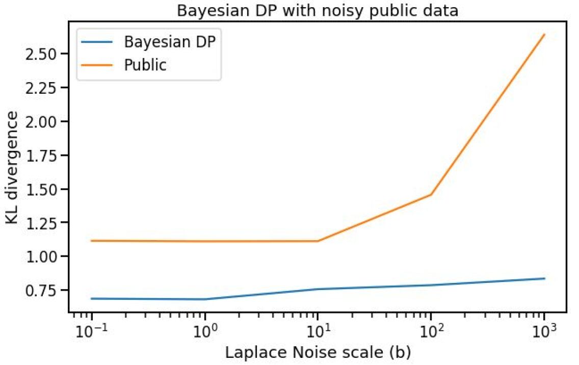
Figure 4: KL-divergence of Bayesian differential privacy vs the scale of the Laplace noise added to the public data to deteriorate its quality. The number of users is 4M, ϵ=0.1italic-ϵ0.1\epsilon=0.1 and |𝒱|=50K𝒱50𝐾|\mathcal{V}|=50K.

4.5 Comparison with K-Anonymity

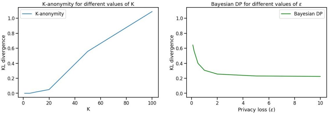
We compare our mechanism to K-anonymity, by evaluating the KL-divergence of the method at different values of K as shown in Figure 5. For ϵ=0.2italic-ϵ0.2\epsilon=0.2, we achieve similar utility to K-anonymity with K=50𝐾50K=50. However, differential privacy offers superior privacy guarantees.
Refer to caption
Figure 5: Left: KL-divergence from the private distribution of K-anonymity vs K. Right: KL-divergence of Bayesian DP vs ϵitalic-ϵ\epsilon. Both plots have the same scale on the y-axis (KL-divergence). The number of users is 100K and vocabulary size is 50K.

4.6 Performance in Language Modeling

We compare the perplexity of our mechanism applied to n-grams in language modeling to the other baselines and K-anonymity. Since the performance of n-gram language models depends on the back-off strategies and how out-of-vocabulary words are handled, we constrain the data to only in-vocabulary words and sentences covered by trigrams so no back-off strategy is required, leading to a fair comparison in as shown in Table 1.

Mechanism Perplexity
Private baseline 29.48
K-anonymity with K = 50 35.51
Bayesian DP at ϵ=0.2italic-ϵ0.2\epsilon=0.2 35.55
Laplace DP + public data at ϵ=0.2italic-ϵ0.2\epsilon=0.2 580.46
Laplace DP at ϵ=0.2italic-ϵ0.2\epsilon=0.2 894.32
Public baseline 43.00
Table 1: Average word perplexity for different mechanisms using trigram language models. The number of distinct n-grams is 60K

5 Empirical Privacy Bounds By Membership Inference Attack

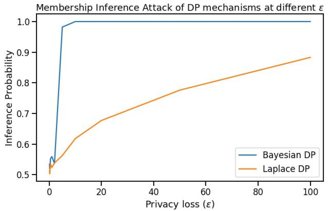
The reason why our Bayesian mechanism is outperforming the standard Laplace mechanism for the same ϵitalic-ϵ\epsilon is because our mechanism has tighter bounds on the privacy loss. This is due to the word-based clipping strategy that minimizes the sensitivity effect of rare words. Moreover, the brute-force method of estimating the sensitivity tied with the hyperparameter tuning allows us to find the optimal privacy vs utility trade-off. To confirm this, we apply a membership inference attack (eval-dp, ) to the output of our Bayesian mechanism and compare against the Laplace mechanism. To perform the attack, we apply the mechanism to two adjacent datasets, one of which does not have the most contributing, in terms of user counts. We then sample two probability distributions 𝜽,𝜽𝒖𝜽subscript𝜽𝒖\boldsymbol{\theta},\boldsymbol{\theta_{-u}} from each dataset and repeat the same process N𝑁N times. The probability of membership inference is then the number of times the KL-divergence, relative to the removed user distribution, of 𝜽𝜽\boldsymbol{\theta} is less than that of 𝜽𝒖subscript𝜽𝒖\boldsymbol{\theta_{-u}} divided by N𝑁N. Plots in Figure 6 show that the probability of membership inference of the Laplace mechanism grows slowly with ϵitalic-ϵ\epsilon, even at ϵ=100italic-ϵ100\epsilon=100 the probability is still less than 0.90.90.9, whereas the inference probability of the Bayesian mechanism approaches 111 as soon as ϵ5italic-ϵ5\epsilon\geq 5. Therefore, the Bayesian mechanism gives a more accurate estimate of the true privacy loss ϵitalic-ϵ\epsilon, since from the definition of differential privacy, a ϵ5italic-ϵ5\epsilon\geq 5 indicates that the ratio between the output probability of the adjacent datasets is >exp(5)148absent5148>\exp(5)\approx 148, which is a clear privacy violation. In other words, the Laplace mechanism is excessively pessimistic about ϵitalic-ϵ\epsilon and it is possible to achieve much higher utility at a lower ϵitalic-ϵ\epsilon using the Bayesian mechanism.

Refer to caption
Figure 6: Membership inference probability vs ϵitalic-ϵ\epsilon for Laplace DP and Bayesian DP. The number of users is 1.2M and the vocabulary size is 50K.

6 Conclusion

In this paper, we proposed a novel Bayesian differential privacy approach, applied to n-grams, which utilises public data to provide a significantly better utility vs privacy trade-off compared to well-known privacy mechanisms, such as the Laplace mechanism. In our approach, we transform the counts to log space, approximating the distribution of the public and private data as Gaussian. The posterior distribution is then evaluated and softmax is applied to produce a probability distribution. We performed several experiments on n-grams from the Reddit dataset to demonstrate the superior performance of our mechanism, achieving up to 85% reduction in KL-divergence compared to the Laplace mechanism for privacy loss ϵ=0.1italic-ϵ0.1\epsilon=0.1, and similar KL-divergence performance to K-anonymity with K=50𝐾50K=50. Finally, we applied a membership inference attack to explain the improvement of our mechanism over the Laplace mechanism. The attack showed that our mechanism provides tighter bounds on the privacy loss and thus gives better estimate of ϵitalic-ϵ\epsilon. Future work will investigate using a similar Bayesian approach to apply differential privacy to deep neural networks during Stochastic Gradient Descent (SGD) training.

Acknowledgements

The authors of this paper would like to acknowledge the SwiftKey Task and Intelligence Research team, in particular Joe Osborne and Dmitry Stratiychuk, for their insights and suggestions that guided the research. We would also like to acknowledge everyone that reviewed this paper and provided invaluable guidance and feedback.

References

  • (1) P. Samarati and L. Sweeney, “Protecting privacy when disclosing information: k-anonymity and its enforcement through generalization and suppression,” 1998.
  • (2) N. Holohan, S. Antonatos, S. Braghin, and P. Mac Aonghusa, “(k,ϵ)𝑘italic-ϵ(k,\epsilon)-anonymity: k-anonymity with ϵitalic-ϵ\epsilon-differential privacy,” arXiv preprint arXiv:1710.01615, 2017.
  • (3) R. Chen, G. Acs, and C. Castelluccia, “Differentially private sequential data publication via variable-length n-grams,” in Proceedings of the 2012 ACM conference on Computer and communications security, pp. 638–649, 2012.
  • (4) S. Gopi, P. Gulhane, J. Kulkarni, J. H. Shen, M. Shokouhi, and S. Yekhanin, “Differentially private set union,” arXiv preprint arXiv:2002.09745, 2020.
  • (5) C. Dimitrakakis, B. Nelson, Z. Zhang, A. Mitrokotsa, and B. I. Rubinstein, “Differential privacy for bayesian inference through posterior sampling,” The Journal of Machine Learning Research, vol. 18, no. 1, pp. 343–381, 2017.
  • (6) C. Dwork and A. Roth, “The algorithmic foundations of differential privacy,” Found. Trends Theor. Comput. Sci., vol. 9, p. 211–407, Aug. 2014.
  • (7) C. Dwork, “Differential privacy, in automata, languages and programming,” ser. Lecture Notes in Computer Scienc, vol. 4052, p. 112, 2006.
  • (8) Y.-X. Wang, S. Fienberg, and A. Smola, “Privacy for free: Posterior sampling and stochastic gradient monte carlo,” in International Conference on Machine Learning, pp. 2493–2502, 2015.
  • (9) D. Klein, “Lecture notes in statistical nlp,” 2008.
  • (10) S. Zheng, “The differential privacy of bayesian inference,” Bachelor’s thesis, Harvard College, 2015.
  • (11) D. J. MacKay, “Choice of basis for laplace approximation,” Machine learning, vol. 33, no. 1, pp. 77–86, 1998.
  • (12) A. Srivastava and C. Sutton, “Autoencoding variational inference for topic models,” arXiv preprint arXiv:1703.01488, 2017.
  • (13) K. Minami, H. Arai, I. Sato, and H. Nakagawa, “Differential privacy without sensitivity,” in Advances in Neural Information Processing Systems, pp. 956–964, 2016.
  • (14) V. Pichapati, A. T. Suresh, F. X. Yu, S. J. Reddi, and S. Kumar, “Adaclip: Adaptive clipping for private sgd,” arXiv preprint arXiv:1908.07643, 2019.
  • (15) J. Liu and K. Talwar, “Private selection from private candidates,” in Proceedings of the 51st Annual ACM SIGACT Symposium on Theory of Computing, pp. 298–309, 2019.
  • (16) K. Ligett, S. Neel, A. Roth, B. Waggoner, and S. Z. Wu, “Accuracy first: Selecting a differential privacy level for accuracy constrained erm,” in Advances in Neural Information Processing Systems, pp. 2566–2576, 2017.
  • (17) C. Chelba, T. Mikolov, M. Schuster, Q. Ge, T. Brants, P. Koehn, and T. Robinson, “One billion word benchmark for measuring progress in statistical language modeling,” tech. rep., Google, 2013.
  • (18) B. Jayaraman and D. Evans, “Evaluating differentially private machine learning in practice,” in 28th {{\{USENIX}}\} Security Symposium ({{\{USENIX}}\} Security 19), pp. 1895–1912, 2019.

Appendix A Proof of Theorem 1 and Corollary 1

We start by proving Theorem 1 where the Gaussian mechanism proposed can be composed into a deterministic function f𝑓f and an additive Gaussian noise 𝜼𝜼\boldsymbol{\eta}.
Define f:𝒩|𝒰|×VV:𝑓superscript𝒩𝒰𝑉superscript𝑉f:\mathcal{N}^{|\mathcal{U}|\times V}\rightarrow\mathbb{R}^{V}, where 𝒰𝒰\mathcal{U} is the set of all private users of a database D𝐷D and V=|𝒱|𝑉𝒱V=|\mathcal{V}| is the vocabulary size. Adopting the same notation used in theorem 1, let Dnsubscript𝐷𝑛D_{-n} be an adjacent database to D𝐷D with user n|𝒰|𝑛𝒰n\in|\mathcal{U}| removed and let 𝜶V,𝚫𝐜(𝐣)Vformulae-sequence𝜶superscript𝑉𝚫superscript𝐜𝐣superscript𝑉\boldsymbol{\alpha}\in\mathbb{R}^{V},\mathbf{\Delta c^{(j)}}\in\mathbb{R}^{V} be the public and user j𝑗j counts respectively. The adjacency, sup(𝐜,𝐜n)𝑠𝑢𝑝𝐜subscript𝐜𝑛sup(\mathbf{c},\mathbf{c}_{-n}), is expressed formally as 𝐜=j|𝒰|𝚫𝐜(j)𝐜superscriptsubscript𝑗𝒰𝚫superscript𝐜𝑗\mathbf{c}=\sum_{j}^{|\mathcal{U}|}\mathbf{\Delta c}^{(j)} and 𝐜n=jn|𝒰|𝚫𝐜(j)subscript𝐜𝑛superscriptsubscript𝑗𝑛𝒰𝚫superscript𝐜𝑗\mathbf{c}_{-n}=\sum_{j\neq n}^{|\mathcal{U}|}\mathbf{\Delta c}^{(j)}. Consequently, :f(𝐜,𝜶,ρ)+𝜼:𝑓𝐜𝜶𝜌𝜼\mathcal{M}:f(\mathbf{c},\boldsymbol{\alpha},\rho)+\boldsymbol{\eta}, where:

f(𝐜,𝜶,ρ)=ρ𝐱^+(1ρ)𝝁p𝑓𝐜𝜶𝜌𝜌^𝐱1𝜌subscript𝝁𝑝\displaystyle f(\mathbf{c},\boldsymbol{\alpha},\rho)=\rho\mathbf{\hat{x}}+(1-\rho)\boldsymbol{\mu}_{p}
𝐱^=log(𝐜+1)1Vlog(𝐜+1)1^𝐱𝐜11𝑉subscriptdelimited-∥∥𝐜11\displaystyle\mathbf{\hat{x}}=\log(\mathbf{c}+1)-\frac{1}{V}\left\lVert\log(\mathbf{c}+1)\right\rVert_{1}
𝝁p=log𝜶1Vlog𝜶1subscript𝝁𝑝𝜶1𝑉subscriptdelimited-∥∥𝜶1\displaystyle\boldsymbol{\mu}_{p}=\log\boldsymbol{\alpha}-\frac{1}{V}\left\lVert\log\boldsymbol{\alpha}\right\rVert_{1}
ηi𝒩(0,σps),iVformulae-sequencesimilar-tosubscript𝜂𝑖𝒩0subscript𝜎𝑝𝑠for-all𝑖𝑉\displaystyle\eta_{i}\sim\mathcal{N}(0,\sigma_{ps}),\forall i\in V

\mathcal{M} satisfies a (ϵ,δitalic-ϵ𝛿\epsilon,\delta)-DP Gaussian mechanism if the standard deviation σps>2log(1.25δ)𝚫2fϵsubscript𝜎𝑝𝑠21.25𝛿subscript𝚫2𝑓italic-ϵ\sigma_{ps}>\sqrt{2\log(\frac{1.25}{\delta})}\frac{\boldsymbol{\Delta}_{2}f}{\epsilon}, where

𝚫2fsubscript𝚫2𝑓\displaystyle\boldsymbol{\Delta}_{2}f =maxsup(𝐜,𝐜n)f(𝐜,𝜶,ρ)f(𝐜n,𝜶,ρ)2\displaystyle=\max_{sup(\mathbf{c},\mathbf{c}_{-n})}\left\lVert f(\mathbf{c},\boldsymbol{\alpha},\rho)-f(\mathbf{c}_{-n},\boldsymbol{\alpha},\rho)\right\rVert_{2}
=maxsup(𝐜,𝐜n)ρ𝐱^+(1ρ)𝝁pρ𝐱^n(1ρ)𝝁p2\displaystyle=\max_{sup(\mathbf{c},\mathbf{c}_{-n})}\left\lVert\rho\mathbf{\hat{x}}+(1-\rho)\boldsymbol{\mu}_{p}-\rho\mathbf{\hat{x}}_{-n}-(1-\rho)\boldsymbol{\mu}_{p}\right\rVert_{2}
=ρmaxsup(𝐜,𝐜n)𝐱^𝐱^n2\displaystyle=\rho\max_{sup(\mathbf{c},\mathbf{c}_{-n})}\left\lVert\mathbf{\hat{x}}-\mathbf{\hat{x}}_{-n}\right\rVert_{2}

And rearranging this will give:

maxsup(𝐜,𝐜n)𝐱^𝐱^n2<ϵσpsρ2log(1.25δ)\max_{sup(\mathbf{c},\mathbf{c}_{-n})}\left\lVert\mathbf{\hat{x}}-\mathbf{\hat{x}}_{-n}\right\rVert_{2}<\frac{\epsilon\sigma_{ps}}{\rho\sqrt{2\log(\frac{1.25}{\delta})}}

Corollary 1 follows from Theorem 1 if we replace 𝐱^^𝐱\mathbf{\hat{x}} with 𝐰𝐱^direct-product𝐰^𝐱\mathbf{w}\odot\mathbf{\hat{x}}, where 𝐰=min[1,𝐍S/C]𝐰1𝐍𝑆𝐶\mathbf{w}=\min[1,\mathbf{N}S/C] as defined by equation 5 and 𝐰n=min[1,(𝐍𝟙(𝚫𝐜n>0))S/C]subscript𝐰𝑛1𝐍1𝚫subscript𝐜𝑛0𝑆𝐶\mathbf{w}_{-n}=\min\Big{[}1,\big{(}\mathbf{N}-\mathbbm{1}(\mathbf{\Delta c}_{-n}>0)\big{)}S/C\Big{]}, since each user can only affect the number of users for any word Nisubscript𝑁𝑖N_{i} by 1. As a result:

𝚫2f/ρsubscript𝚫2𝑓𝜌\displaystyle\boldsymbol{\Delta}_{2}f/\rho =maxsup(𝐜,𝐜n)𝐰𝐱^𝐰n𝐱^n2\displaystyle=\max_{sup(\mathbf{c},\mathbf{c}_{-n})}\left\lVert\mathbf{w}\odot\mathbf{\hat{x}}-\mathbf{w}_{-n}\odot\mathbf{\hat{x}}_{-n}\right\rVert_{2}
=maxsup(𝐜,𝐜n)𝐰(𝐱^𝐱^n)+(𝐰𝐰n)𝐱^n2\displaystyle=\max_{sup(\mathbf{c},\mathbf{c}_{-n})}\left\lVert\mathbf{w}\odot(\mathbf{\hat{x}}-\mathbf{\hat{x}}_{-n})+(\mathbf{w}-\mathbf{w}_{-n})\odot\mathbf{\hat{x}}_{-n}\right\rVert_{2}
=maxsup(𝐜,𝐜n)𝐰𝚫𝐱^+SC𝟙(𝐍CS)𝐱^n2\displaystyle=\max_{sup(\mathbf{c},\mathbf{c}_{-n})}\left\lVert\mathbf{w}\odot\mathbf{\Delta\hat{x}}+\frac{S}{C}\mathbbm{1}\Big{(}\mathbf{N}\leq\frac{C}{S}\Big{)}\odot\mathbf{\hat{x}}_{-n}\right\rVert_{2}

The identity function in the last equality stems from clamping the decay function at 111, i.e the gradient is zero for 𝐍S/C>1𝐍𝑆𝐶1\mathbf{N}S/C>1 or 𝐍>C/S𝐍𝐶𝑆\mathbf{N}>C/S. We note also that the first equality can be rearranged differently, which will come handy in the proving claim 1, as follows:

maxsup(𝐜,𝐜n)𝐰n𝐱^𝐰n𝐱^n2\displaystyle\max_{sup(\mathbf{c},\mathbf{c}_{-n})}\left\lVert\mathbf{w}_{-n}\odot\mathbf{\hat{x}}-\mathbf{w}_{-n}\odot\mathbf{\hat{x}}_{-n}\right\rVert_{2} =maxsup(𝐜,𝐜n)𝐰n(𝐱^𝐱^n)+(𝐰𝐰n)𝐱^2\displaystyle=\max_{sup(\mathbf{c},\mathbf{c}_{-n})}\left\lVert\mathbf{w}_{-n}\odot(\mathbf{\hat{x}}-\mathbf{\hat{x}}_{-n})+(\mathbf{w}-\mathbf{w}_{-n})\odot\mathbf{\hat{x}}\right\rVert_{2}
=maxsup(𝐜,𝐜n)𝐰n𝚫𝐱^+SC𝟙(𝐍CS)𝐱^2\displaystyle=\max_{sup(\mathbf{c},\mathbf{c}_{-n})}\left\lVert\mathbf{w}_{-n}\odot\mathbf{\Delta\hat{x}}+\frac{S}{C}\mathbbm{1}\Big{(}\mathbf{N}\leq\frac{C}{S}\Big{)}\odot\mathbf{\hat{x}}\right\rVert_{2} (7)

Appendix B Proof of Claim 1

Claim 1 provides a worst-case estimate of the sensitivity 𝚫𝝁ps2subscriptdelimited-∥∥𝚫subscript𝝁𝑝𝑠2\left\lVert\boldsymbol{\Delta\mu}_{ps}\right\rVert_{2}, that does not require recomputing sensitivity of Dnsubscript𝐷𝑛D_{-n} for each user n𝑛n. Firstly, we state the following lemma:

Lemma 1.

The sensitivity |𝚫𝐱^|𝚫^𝐱|\mathbf{\Delta\hat{x}}| of 𝐱^^𝐱\mathbf{\hat{x}}, which is defined in equation 2, is bounded from above as follows:

|𝚫𝐱^|𝐋C𝚫^𝐱𝐋𝐶\displaystyle|\mathbf{\Delta\hat{x}}|\leq\mathbf{L}C
Li=(11V)1Ni+jiV1VNjsubscript𝐿𝑖11𝑉1subscript𝑁𝑖superscriptsubscript𝑗𝑖𝑉1𝑉subscript𝑁𝑗\displaystyle L_{i}=\big{(}1-\frac{1}{V}\big{)}\frac{1}{N_{i}}+\sum_{j\neq i}^{V}\frac{1}{VN_{j}}

Then, using this lemma, we start the proof from Equation 7:

maxsup(𝐜,𝐜n)𝐰n𝚫𝐱^+SC𝟙(𝐍CS)𝐱^2\displaystyle\max_{sup(\mathbf{c},\mathbf{c}_{-n})}\left\lVert\mathbf{w}_{-n}\odot\mathbf{\Delta\hat{x}}+\frac{S}{C}\mathbbm{1}\Big{(}\mathbf{N}\leq\frac{C}{S}\Big{)}\odot\mathbf{\hat{x}}\right\rVert_{2} maxsup(𝐜,𝐜n)𝐰n|𝚫𝐱^|+SC𝟙(𝐍CS)|𝐱^|2\displaystyle\leq\max_{sup(\mathbf{c},\mathbf{c}_{-n})}\left\lVert\mathbf{w}_{-n}\odot|\mathbf{\Delta\hat{x}}|+\frac{S}{C}\mathbbm{1}\Big{(}\mathbf{N}\leq\frac{C}{S}\Big{)}\odot|\mathbf{\hat{x}}|\right\rVert_{2}
maxsup(𝐜,𝐜n)𝐰|𝚫𝐱^|+SC𝟙(𝐍CS)|𝐱^|2\displaystyle\leq\max_{sup(\mathbf{c},\mathbf{c}_{-n})}\left\lVert\mathbf{w}\odot|\mathbf{\Delta\hat{x}}|+\frac{S}{C}\mathbbm{1}\Big{(}\mathbf{N}\leq\frac{C}{S}\Big{)}\odot|\mathbf{\hat{x}}|\right\rVert_{2}
𝐰𝐋C+SC𝟙(𝐍CS)|𝐱^|2absentsubscriptdelimited-∥∥direct-product𝐰𝐋𝐶direct-product𝑆𝐶1𝐍𝐶𝑆^𝐱2\displaystyle\leq\left\lVert\mathbf{w}\odot\mathbf{L}C+\frac{S}{C}\mathbbm{1}\Big{(}\mathbf{N}\leq\frac{C}{S}\Big{)}\odot|\mathbf{\hat{x}}|\right\rVert_{2}

The last two inequalities follow from the monotonicity of 𝐰𝐰\mathbf{w} and Lemma 1 respectively.
Now we prove Lemma 1, by defining a strictly increasing function 𝐲^^𝐲\mathbf{\hat{y}} similar to 𝐱^^𝐱\mathbf{\hat{x}}:

y^i=log(ci+1)(11V)+jilog(cj+1),iVformulae-sequencesubscript^𝑦𝑖subscript𝑐𝑖111𝑉subscript𝑗𝑖subscript𝑐𝑗1𝑖𝑉\hat{y}_{i}=\log(c_{i}+1)(1-\frac{1}{V})+\sum_{j\neq i}\log(c_{j}+1),i\in V

The function y^i(𝐜)subscript^𝑦𝑖𝐜\hat{y}_{i}(\mathbf{c}) has two important properties:

  • It is a concave function, since it’s a strictly increasing linear combination of log\log

  • |Δx^i||Δy^i|Δsubscript^𝑥𝑖Δsubscript^𝑦𝑖|\Delta\hat{x}_{i}|\leq|\Delta\hat{y}_{i}|

From the first property we can conclude that y^isubscript^𝑦𝑖\hat{y}_{i} is Lisubscript𝐿𝑖L_{i}-Lipschitz over 𝐜𝐜\mathbf{c} with respect to the .\left\lVert.\right\rVert_{\infty} if y^i1Lisubscriptdelimited-∥∥subscript^𝑦𝑖1subscript𝐿𝑖\left\lVert\nabla\hat{y}_{i}\right\rVert_{1}\leq L_{i}, since l1subscript𝑙1l_{1} and lsubscript𝑙l_{\infty} are dual norms. Moreover:

y^icjsubscript^𝑦𝑖subscript𝑐𝑗\displaystyle\frac{\partial\hat{y}_{i}}{\partial c_{j}} ={(11V)1cj+1j=i1V(cj+1)jiabsentcases11𝑉1subscript𝑐𝑗1𝑗𝑖1𝑉subscript𝑐𝑗1𝑗𝑖\displaystyle=\begin{cases}(1-\frac{1}{V})\frac{1}{c_{j}+1}&j=i\\ \frac{1}{V(c_{j}+1)}&j\neq i\end{cases}
{(11V)1Nj+1j=i1V(Nj+1)jiabsentcases11𝑉1subscript𝑁𝑗1𝑗𝑖1𝑉subscript𝑁𝑗1𝑗𝑖\displaystyle\leq\begin{cases}(1-\frac{1}{V})\frac{1}{N_{j}+1}&j=i\\ \frac{1}{V(N_{j}+1)}&j\neq i\end{cases}

The inequality follows because the smallest word count is equal to the number of users that have the word. Consequently, the maximum l1subscript𝑙1l_{1} norm of the gradient: Li=(11V)1Ni+jiV1VNjsubscript𝐿𝑖11𝑉1subscript𝑁𝑖superscriptsubscript𝑗𝑖𝑉1𝑉subscript𝑁𝑗L_{i}=\big{(}1-\frac{1}{V}\big{)}\frac{1}{N_{i}}+\sum_{j\neq i}^{V}\frac{1}{VN_{j}}. From the Lipschitz property:

|Δx^i||Δy^i|=|y^i(𝐜)y^i(𝐜n)|Li𝐜𝐜nLiC,iVformulae-sequenceΔsubscript^𝑥𝑖Δsubscript^𝑦𝑖subscript^𝑦𝑖𝐜subscript^𝑦𝑖subscript𝐜𝑛subscript𝐿𝑖subscriptdelimited-∥∥𝐜subscript𝐜𝑛subscript𝐿𝑖𝐶𝑖𝑉|\Delta\hat{x}_{i}|\leq|\Delta\hat{y}_{i}|=|\hat{y}_{i}(\mathbf{c})-\hat{y}_{i}(\mathbf{c}_{-n})|\leq L_{i}\left\lVert\mathbf{c}-\mathbf{c}_{-n}\right\rVert_{\infty}\leq L_{i}C,i\in V
|𝚫𝐱^|𝐋C𝚫^𝐱𝐋𝐶|\mathbf{\Delta\hat{x}}|\leq\mathbf{L}C

Appendix C Proof of Theorem 2

The first part of the theorem is a variant of the noisy max algorithm, with the relaxation that the score function does not have to be monotonic. To follow the same steps as the noisy max proof, we will prove the theorem for the maximum of the negative score function q𝑞q. This is allowed because of the symmetry of the Laplace noise.

Let sk=q(𝐜,𝝁𝒑𝒔(𝒌))subscript𝑠𝑘𝑞𝐜superscriptsubscript𝝁𝒑𝒔𝒌s_{k}=-q(\mathbf{c},\boldsymbol{\mu_{ps}^{(k)}}) and sk=q(𝐜n,𝝁𝒑𝒔(𝒌)n)superscriptsubscript𝑠𝑘𝑞subscript𝐜𝑛subscriptsuperscriptsubscript𝝁𝒑𝒔𝒌𝑛s_{k}^{\prime}=-q(\mathbf{c}_{-n},\boldsymbol{\mu_{ps}^{(k)}}_{-n}) be the scores for the adjacent databases D,Dn𝐷subscript𝐷𝑛D,D_{-n} for n|𝒰|for-all𝑛𝒰\forall n\in|\mathcal{U}| and kK𝑘𝐾k\in K. For any kK𝑘𝐾k\in K, fix 𝜼ksubscript𝜼𝑘\boldsymbol{\eta}_{-k}, a draw from [Lap(2|Δq|/ϵ)]K1superscriptdelimited-[]𝐿𝑎𝑝2Δ𝑞italic-ϵ𝐾1\big{[}Lap(2|\Delta q|/\epsilon)\big{]}^{K-1} used for all noisy scores except the kth score. We will argue for each 𝜼ksubscript𝜼𝑘\boldsymbol{\eta}_{-k} independently.
Define the notation P(k|ζ)𝑃conditional𝑘𝜁P(k|\zeta) to mean the probability that the output of the mechanism (index of the maximum noisy score) is k𝑘k, conditioned on ζ𝜁\zeta.
First, we show that P(k|D,𝜼k)eϵP(k|Dn,𝜼k),n|𝒰|formulae-sequence𝑃conditional𝑘𝐷subscript𝜼𝑘superscript𝑒italic-ϵ𝑃conditional𝑘subscript𝐷𝑛subscript𝜼𝑘for-all𝑛𝒰P(k|D,\boldsymbol{\eta}_{-k})\leq e^{\epsilon}P(k|D_{-n},\boldsymbol{\eta}_{-k}),\forall n\in|\mathcal{U}|. Define

η=minηksk+ηk>sm+ηmmksuperscript𝜂subscriptsubscript𝜂𝑘subscript𝑠𝑘subscript𝜂𝑘subscript𝑠𝑚subscript𝜂𝑚for-all𝑚𝑘\eta^{*}=\min_{\eta_{k}}s_{k}+\eta_{k}>s_{m}+\eta_{m}\;\forall m\neq k

Since we want the maximum value, k𝑘k will be the output when the database is D𝐷D if and only if ηkηsubscript𝜂𝑘superscript𝜂\eta_{k}\geq\eta^{*}. Let Δsi=sisiiKΔsubscript𝑠𝑖subscript𝑠𝑖subscriptsuperscript𝑠𝑖for-all𝑖𝐾\Delta s_{i}=s_{i}-s^{\prime}_{i}\;\forall i\in K, we have for all 1mkK1𝑚𝑘𝐾1\leq m\neq k\leq K:

sk+ηsubscript𝑠𝑘superscript𝜂\displaystyle s_{k}+\eta^{*} >sm+ηmabsentsubscript𝑠𝑚subscript𝜂𝑚\displaystyle>s_{m}+\eta_{m}
sk+Δsk+ηsubscriptsuperscript𝑠𝑘Δsubscript𝑠𝑘superscript𝜂\displaystyle s^{\prime}_{k}+\Delta s_{k}+\eta^{*} >sm+Δsm+ηmabsentsubscriptsuperscript𝑠𝑚Δsubscript𝑠𝑚subscript𝜂𝑚\displaystyle>s^{\prime}_{m}+\Delta s_{m}+\eta_{m}
sk+2|Δq|+ηsk+subscriptsuperscript𝑠𝑘2Δ𝑞superscript𝜂limit-fromsubscriptsuperscript𝑠𝑘\displaystyle s^{\prime}_{k}+2|\Delta q|+\eta^{*}\geq s^{\prime}_{k}+ ΔskΔsm+η>sm+ηmΔsubscript𝑠𝑘Δsubscript𝑠𝑚superscript𝜂subscriptsuperscript𝑠𝑚subscript𝜂𝑚\displaystyle\Delta s_{k}-\Delta s_{m}+\eta^{*}>s^{\prime}_{m}+\eta_{m}

Thus, if ηk2|Δq|+ηsubscript𝜂𝑘2Δ𝑞superscript𝜂\eta_{k}\geq 2|\Delta q|+\eta^{*}, then the kth score will be the maximum when the database is Dn,n|𝒰|subscript𝐷𝑛for-all𝑛𝒰D_{-n},\;\forall n\in|\mathcal{U}| and the noise vector is (ηk,𝜼k)subscript𝜂𝑘subscript𝜼𝑘(\eta_{k},\boldsymbol{\eta}_{-k}). The probabilities below are over the choice of ηkLap(2|Δq|/ϵ|)\eta_{k}\sim Lap(2|\Delta q|/\epsilon|):

P(ηk2|Δq|+η)eϵP(ηkη)=eϵP(k|D,𝜼k)𝑃subscript𝜂𝑘2Δ𝑞superscript𝜂superscript𝑒italic-ϵ𝑃subscript𝜂𝑘superscript𝜂superscript𝑒italic-ϵ𝑃conditional𝑘𝐷subscript𝜼𝑘\displaystyle P(\eta_{k}\geq 2|\Delta q|+\eta^{*})\geq e^{-\epsilon}P(\eta_{k}\geq\eta^{*})=e^{-\epsilon}P(k|D,\boldsymbol{\eta}_{-k})
P(k|Dn,𝜼k)𝑃conditional𝑘subscript𝐷𝑛subscript𝜼𝑘absent\displaystyle P(k|D_{-n},\boldsymbol{\eta}_{-k})\geq P(ηk2|Δq|+η)eϵP(ηkη)=eϵP(k|D,𝜼k)𝑃subscript𝜂𝑘2Δ𝑞superscript𝜂superscript𝑒italic-ϵ𝑃subscript𝜂𝑘superscript𝜂superscript𝑒italic-ϵ𝑃conditional𝑘𝐷subscript𝜼𝑘\displaystyle P(\eta_{k}\geq 2|\Delta q|+\eta^{*})\geq e^{-\epsilon}P(\eta_{k}\geq\eta^{*})=e^{-\epsilon}P(k|D,\boldsymbol{\eta}_{-k})

Rearranging and multiplying both sides by eϵsuperscript𝑒italic-ϵe^{\epsilon}:

P(k|D,𝜼k)eϵP(k|Dn,𝜼k)n|𝒰|𝑃conditional𝑘𝐷subscript𝜼𝑘superscript𝑒italic-ϵ𝑃conditional𝑘subscript𝐷𝑛subscript𝜼𝑘for-all𝑛𝒰P(k|D,\boldsymbol{\eta}_{-k})\leq e^{\epsilon}P(k|D_{-n},\boldsymbol{\eta}_{-k})\;\forall n\in|\mathcal{U}|

Now we show P(k|Dn,𝜼k)eϵP(k|D,𝜼k)n|𝒰|𝑃conditional𝑘subscript𝐷𝑛subscript𝜼𝑘superscript𝑒italic-ϵ𝑃conditional𝑘𝐷subscript𝜼𝑘for-all𝑛𝒰P(k|D_{-n},\boldsymbol{\eta}_{-k})\leq e^{\epsilon}P(k|D,\boldsymbol{\eta}_{-k})\;\forall n\in|\mathcal{U}|, following similar steps as above. Define

η=minηksk+ηk>sm+ηmmksuperscript𝜂subscriptsubscript𝜂𝑘superscriptsubscript𝑠𝑘subscript𝜂𝑘superscriptsubscript𝑠𝑚subscript𝜂𝑚for-all𝑚𝑘\eta^{*}=\min_{\eta_{k}}s_{k}^{\prime}+\eta_{k}>s_{m}^{\prime}+\eta_{m}\;\forall m\neq k

k𝑘k will be the output(argmax noisy score) when the database is Dnn|𝒰|subscript𝐷𝑛for-all𝑛𝒰D_{-n}\;\forall n\in|\mathcal{U}| if and only if ηkηsubscript𝜂𝑘superscript𝜂\eta_{k}\geq\eta^{*} we have for all 1mkK1𝑚𝑘𝐾1\leq m\neq k\leq K:

sk+ηsubscriptsuperscript𝑠𝑘superscript𝜂\displaystyle s^{\prime}_{k}+\eta^{*} >sm+ηmabsentsubscriptsuperscript𝑠𝑚subscript𝜂𝑚\displaystyle>s^{\prime}_{m}+\eta_{m}
sk+Δsk+Δsm+ηsubscriptsuperscript𝑠𝑘Δsubscript𝑠𝑘Δsubscript𝑠𝑚superscript𝜂\displaystyle s^{\prime}_{k}+\Delta s_{k}+\Delta s_{m}+\eta^{*} >sm+Δsk+Δsm+ηmabsentsubscriptsuperscript𝑠𝑚Δsubscript𝑠𝑘Δsubscript𝑠𝑚subscript𝜂𝑚\displaystyle>s^{\prime}_{m}+\Delta s_{k}+\Delta s_{m}+\eta_{m}
sk+2|Δq|+ηsk+subscript𝑠𝑘2Δ𝑞superscript𝜂limit-fromsubscript𝑠𝑘\displaystyle s_{k}+2|\Delta q|+\eta^{*}\geq s_{k}+ ΔsmΔsk+η>sm+ηmΔsubscript𝑠𝑚Δsubscript𝑠𝑘superscript𝜂subscript𝑠𝑚subscript𝜂𝑚\displaystyle\Delta s_{m}-\Delta s_{k}+\eta^{*}>s_{m}+\eta_{m}

Thus, if ηk2|Δq|+ηsubscript𝜂𝑘2Δ𝑞superscript𝜂\eta_{k}\geq 2|\Delta q|+\eta^{*}, then the kth score will be the maximum when the database is D𝐷D and the noise vector is (ηk,𝜼k)subscript𝜂𝑘subscript𝜼𝑘(\eta_{k},\boldsymbol{\eta}_{-k}). The probabilities below are over the choice of ηkLap(2|Δq|/ϵ|)\eta_{k}\sim Lap(2|\Delta q|/\epsilon|):

P(ηk2|Δq|+η)eϵP(ηkη)=eϵP(k|Dn,𝜼k)𝑃subscript𝜂𝑘2Δ𝑞superscript𝜂superscript𝑒italic-ϵ𝑃subscript𝜂𝑘superscript𝜂superscript𝑒italic-ϵ𝑃conditional𝑘subscript𝐷𝑛subscript𝜼𝑘\displaystyle P(\eta_{k}\geq 2|\Delta q|+\eta^{*})\geq e^{-\epsilon}P(\eta_{k}\geq\eta^{*})=e^{-\epsilon}P(k|D_{-n},\boldsymbol{\eta}_{-k})
P(k|D,𝜼k)𝑃conditional𝑘𝐷subscript𝜼𝑘absent\displaystyle P(k|D,\boldsymbol{\eta}_{-k})\geq P(ηk2|Δq|+η)eϵP(ηkη)=eϵP(k|Dn,𝜼k)𝑃subscript𝜂𝑘2Δ𝑞superscript𝜂superscript𝑒italic-ϵ𝑃subscript𝜂𝑘superscript𝜂superscript𝑒italic-ϵ𝑃conditional𝑘subscript𝐷𝑛subscript𝜼𝑘\displaystyle P(\eta_{k}\geq 2|\Delta q|+\eta^{*})\geq e^{-\epsilon}P(\eta_{k}\geq\eta^{*})=e^{-\epsilon}P(k|D_{-n},\boldsymbol{\eta}_{-k})

And so:

P(k|Dn,𝜼k)eϵP(k|D,𝜼k)n|𝒰|𝑃conditional𝑘subscript𝐷𝑛subscript𝜼𝑘superscript𝑒italic-ϵ𝑃conditional𝑘𝐷subscript𝜼𝑘for-all𝑛𝒰P(k|D_{-n},\boldsymbol{\eta}_{-k})\leq e^{\epsilon}P(k|D,\boldsymbol{\eta}_{-k})\;\forall n\in|\mathcal{U}|

Finally, since:

k=argminkK[qkeLap(ϵ2|Δq|)]=argmaxkK[qk+eLap(ϵ2|Δq|)]superscript𝑘𝑎𝑟𝑔𝑚𝑖subscript𝑛𝑘𝐾delimited-[]similar-tosubscript𝑞𝑘𝑒𝐿𝑎𝑝italic-ϵ2Δ𝑞𝑎𝑟𝑔𝑚𝑎subscript𝑥𝑘𝐾delimited-[]similar-tosubscript𝑞𝑘𝑒𝐿𝑎𝑝italic-ϵ2Δ𝑞k^{*}=argmin_{k\in K}\Big{[}q_{k}-e\sim Lap\big{(}\frac{\epsilon}{2|\Delta q|}\big{)}\Big{]}=argmax_{k\in K}\Big{[}-q_{k}+e\sim Lap\big{(}\frac{\epsilon}{2|\Delta q|}\big{)}\Big{]}

which is ϵitalic-ϵ\epsilon-differentially private, it is trivial to show that k=argminkK[qk+eLap(ϵ2|Δq|)]superscript𝑘𝑎𝑟𝑔𝑚𝑖subscript𝑛𝑘𝐾delimited-[]similar-tosubscript𝑞𝑘𝑒𝐿𝑎𝑝italic-ϵ2Δ𝑞k^{*}=argmin_{k\in K}\Big{[}q_{k}+e\sim Lap\big{(}\frac{\epsilon}{2|\Delta q|}\big{)}\Big{]} is also ϵitalic-ϵ\epsilon-differentially private, because the Laplace distribution is symmetric around 00 and the above proof only requires the sensitivity of q𝑞q and no other assumption is made on the properties of q𝑞q.

The second part of the theorem is a direct consequence of having non-overlapping private sets, i.e any user removed in D,Dn𝐷subscript𝐷𝑛D,D_{-n} can only be from one of the private sets and not the other, thus we can treat each set separately and take the maximum sensitivity of both.

Appendix D Proof of Claim 2

The sensitivity with respect to the first private set, (𝐜,𝐜n)𝐜subscript𝐜𝑛(\mathbf{c},\mathbf{c}_{-n}), is a brute-force evaluation of adding and removing each user in the set. This is bounded for all users if you take the maximum word count in the set C1subscript𝐶1C_{1} as shown in the claim. Therefore, here we prove the upper bound of the sensitivity with respect to the second private set (𝝁𝒑𝒔,𝝁𝒑𝒔n)subscript𝝁𝒑𝒔subscriptsubscript𝝁𝒑𝒔𝑛(\boldsymbol{\mu_{ps}},\boldsymbol{\mu_{ps}}_{-n}).
Let 𝐫=𝐰𝐱^𝐫direct-product𝐰^𝐱\mathbf{r}=\mathbf{w}\odot\mathbf{\hat{x}} so 𝝁𝒑𝒔=ρ𝐫+(1ρ)𝝁𝒑subscript𝝁𝒑𝒔𝜌𝐫1𝜌subscript𝝁𝒑\boldsymbol{\mu_{ps}}=\rho\mathbf{r}+(1-\rho)\boldsymbol{\mu_{p}}. We first note that score function q(.,.)q(.,.) defined in equation 6 is a convex function in 𝐫𝐫\mathbf{r} since it is a scaled version of KL-divergence. Consequently, q(.,.)q(.,.) is l𝑙l-Lipschitz over 𝐫𝐫\mathbf{r} with respect to the l2subscript𝑙2l_{2} norm if q2lsubscriptdelimited-∥∥𝑞2𝑙\left\lVert\nabla q\right\rVert_{2}\leq l, since l2subscript𝑙2l_{2} is self-dual. Moreover, for all iV𝑖𝑉i\in V:

|qri|𝑞subscript𝑟𝑖\displaystyle\Big{|}\frac{\partial q}{\partial r_{i}}\Big{|} =|ci(ρρexp(ρri+(1ρ)μpi)j=1Vexp(ρrj+(1ρ)μpj))|absentsubscript𝑐𝑖𝜌𝜌𝜌subscript𝑟𝑖1𝜌subscript𝜇𝑝𝑖superscriptsubscript𝑗1𝑉𝜌subscript𝑟𝑗1𝜌subscript𝜇𝑝𝑗\displaystyle=\bigg{|}c_{i}\Big{(}\rho-\frac{\rho\exp\big{(}\rho r_{i}+(1-\rho)\mu_{pi}\big{)}}{\sum_{j=1}^{V}\exp\big{(}\rho r_{j}+(1-\rho)\mu_{pj}\big{)}}\Big{)}\bigg{|}
=|ciρ(1θi)|θi[0,1]absentsubscript𝑐𝑖𝜌1subscript𝜃𝑖subscript𝜃𝑖01\displaystyle=\big{|}c_{i}\rho(1-\theta_{i})\big{|}\;\;\theta_{i}\in[0,1]
ciρabsentsubscript𝑐𝑖𝜌\displaystyle\leq c_{i}\rho

Thus q(.,.)q(.,.) is l𝑙l-Lipschitz with l=ρ𝐜2𝑙𝜌subscriptdelimited-∥∥𝐜2l=\rho\left\lVert\mathbf{c}\right\rVert_{2}. The Lipschitz property implies that:
|q(𝐜,ρ𝐫+(1ρ)𝝁𝒑)q(𝐜,ρ𝐫n+(1ρ)𝝁𝒑)|ρc2𝚫𝐫2=ρc2𝚫𝝁𝒑𝒔2𝑞𝐜𝜌𝐫1𝜌subscript𝝁𝒑𝑞𝐜𝜌subscript𝐫𝑛1𝜌subscript𝝁𝒑𝜌subscriptdelimited-∥∥𝑐2subscriptdelimited-∥∥𝚫𝐫2𝜌subscriptdelimited-∥∥𝑐2subscriptdelimited-∥∥𝚫subscript𝝁𝒑𝒔2\Big{|}q(\mathbf{c},\rho\mathbf{r}+(1-\rho)\boldsymbol{\mu_{p}})-q(\mathbf{c},\rho\mathbf{r}_{-n}+(1-\rho)\boldsymbol{\mu_{p}})\Big{|}\leq\rho\left\lVert c\right\rVert_{2}\left\lVert\mathbf{\Delta r}\right\rVert_{2}=\rho\left\lVert c\right\rVert_{2}\left\lVert\boldsymbol{\Delta\mu_{ps}}\right\rVert_{2} n|𝒰1|for-all𝑛subscript𝒰1\forall n\in|\mathcal{U}_{1}|