A Comprehensive Survey and Experimental Comparison of Graph-Based Approximate Nearest Neighbor Search

Abstract.

Approximate nearest neighbor search (ANNS) constitutes an important operation in a multitude of applications, including recommendation systems, information retrieval, and pattern recognition. In the past decade, graph-based ANNS algorithms have been the leading paradigm in this domain, with dozens of graph-based ANNS algorithms proposed. Such algorithms aim to provide effective, efficient solutions for retrieving the nearest neighbors for a given query. Nevertheless, these efforts focus on developing and optimizing algorithms with different approaches, so there is a real need for a comprehensive survey about the approaches’ relative performance, strengths, and pitfalls. Thus here we provide a thorough comparative analysis and experimental evaluation of 13 representative graph-based ANNS algorithms via a new taxonomy and fine-grained pipeline. We compared each algorithm in a uniform test environment on eight real-world datasets and 12 synthetic datasets with varying sizes and characteristics. Our study yields novel discoveries, offerings several useful principles to improve algorithms, thus designing an optimized method that outperforms the state-of-the-art algorithms. This effort also helped us pinpoint algorithms’ working portions, along with rule-of-thumb recommendations about promising research directions and suitable algorithms for practitioners in different fields.

PVLDB Reference Format:
Mengzhao Wang, Xiaoliang Xu, Qiang Yue, Yuxiang Wang. A Comprehensive Survey and Experimental Comparison of Graph-Based Approximate Nearest Neighbor Search. PVLDB, 14(1): XXX-XXX, 2021.
doi:XX.XX/XXX.XX

PVLDB Artifact Availability:
The source code, data, and/or other artifacts have been made available at %leave␣empty␣if␣no␣availability␣url␣should␣be␣sethttps://github.com/Lsyhprum/WEAVESS.

1. Introduction

Nearest Neighbor Search (NNS) is a fundamental building block in various application domains (Milvus, 2019; Fu et al., 2019; Malkov and Yashunin, 2018; Riegger, 2010; Arora et al., 2018; Aoyama et al., 2011; Zhang and He, 2018; Zhou et al., 2013), such as information retrieval (Flickner et al., 1995; Zhu et al., 2019), pattern recognition (Kosuge and Oshima, 2019; Cover and Hart, 1967), data mining (Iwasaki, 2016; Huang et al., 2017), machine learning (Cost and Salzberg, 1993; Cao et al., 2017), and recommendation systems (Sarwar et al., 2001; Meng et al., 2020). With the explosive growth of datasets’ scale and the inevitable curse of dimensionality, accurate NNS cannot meet actual requirements for efficiency and cost (Li et al., 2019). Thus, much of the literature has focused on efforts to research approximate NNS (ANNS) and find an algorithm that improves efficiency substantially while mildly relaxing accuracy constraints (an accuracy-versus-efficiency tradeoff (Li et al., 2020)).

ANNS is a task that finds the approximate nearest neighbors among a high-dimensional dataset for a query via a well-designed index. According to the index adopted, the existing ANNS algorithms can be divided into four major types: hashing-based (Gong et al., 2020; Huang et al., 2015); tree-based (Silpa-Anan and Hartley, 2008; Arora et al., 2018); quantization-based (Jegou et al., 2010; Pan et al., 2020); and graph-based (Malkov and Yashunin, 2018; Fu et al., 2019) algorithms. Recently, graph-based algorithms have emerged as a highly effective option for ANNS (Aumüller et al., 2017; Aoyama et al., 2013; Hacid and Yoshida, 2010; Paredes and Chávez, 2005). Thanks to graph-based ANNS algorithms’ extraordinary ability to express neighbor relationships (Fu et al., 2019; Weber et al., 1998), they only need to evaluate fewer points of dataset to receive more accurate results (Malkov and Yashunin, 2018; Fu et al., 2019; Li et al., 2019; Zhao et al., 2019b; Munoz et al., 2019).

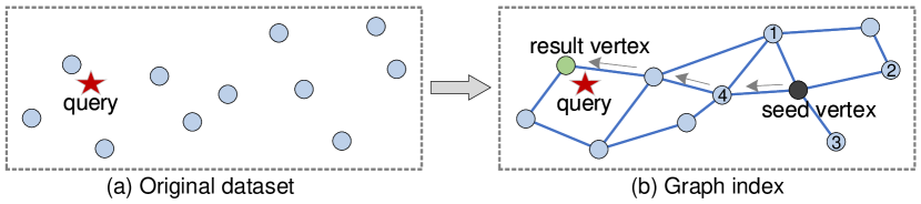
Figure 1. A toy example for the graph-based ANNS algorithm.

As Figure 1 shows, graph-based ANNS algorithms build a graph index (Figure 1(b)) on the original dataset (Figure 1(a)), the vertices in the graph correspond to the points of the original dataset, and neighboring vertices (marked as $x$, $y$) are associated with an edge by evaluating their distance $\delta(x,y)$, where $\delta$ is a distance function. In Figure 1(b), the four vertices (numbered 1–4) connected to the black vertex are its neighbors, and the black vertex can visit its neighbors along these edges. Given this graph index and a query $q$ (the red star), ANNS aims to get a set of vertices that are close to $q$. We take the case of returning $q$’s nearest neighbor as an example to show ANNS’ general procedure: Initially, a seed vertex (the black vertex, it can be randomly sampled or obtained by additional approaches (Malkov and Yashunin, 2018; Iwasaki, 2016)) is selected as the result vertex $r$, and we can conduct ANNS from this seed vertex. Specifically, if $\delta(n,q)<\delta(r,q)$, where $n$ is one of the neighbors of $r$, $r$ will be replaced by ${n}$. We repeat this process until the termination condition (e.g., $\forall{n},\delta(n,q)\geq\delta(r,q)$) is met, and the final ${r}$ (the green vertex) is $q$’s nearest neighbor. Compared with other index structures, graph-based algorithms are a proven superior tradeoff in terms of accuracy versus efficiency  (Aumüller et al., 2017; Malkov et al., 2014; Malkov and Yashunin, 2018; Li et al., 2019; Fu et al., 2019), which is probably why they enjoy widespread use among high-tech companies nowadays (e.g., Microsoft (Wang and Li, 2012; Wang et al., 2012), Alibaba (Zhao et al., 2019b; Fu et al., 2019), and Yahoo (Sugawara et al., 2016; Iwasaki, 2016; Iwasaki and Miyazaki, 2018)).

1.1. Motivation

The problem of graph-based ANNS on high-dimensional and large-scale data has been studied intensively across the literature (Fu et al., 2019). Dozens of algorithms have been proposed to solve this problem from different optimizations (Malkov et al., 2014; Malkov and Yashunin, 2018; Harwood and Drummond, 2016; Fu et al., 2021; Munoz et al., 2019; Jin et al., 2014; Fu and Cai, 2016). For these algorithms, existing surveys (Aumüller et al., 2017; Li et al., 2019; Shimomura et al., 2020) provide some meaningful explorations. However, they are limited to a small subset about algorithms, datasets, and metrics, as well as studying algorithms from a macro perspective, and the analysis and evaluation of intra-algorithm components are ignored. For example, (Li et al., 2019) includes a few graph-based algorithms (only three), (Aumüller et al., 2017) focuses on efficiency vs accuracy tradeoff, (Shimomura et al., 2020) only considers several classic graphs. This motivates us to carry out a thorough comparative analysis and experimental evaluation of existing graph-based algorithms via a new taxonomy and micro perspective (i.e., some fine-grained components). We detail the issues of existing work that ensued.

I1: Lack of a reasonable taxonomy and comparative analysis of inter-algorithms. Many studies in other fields show that an insightful taxonomy can serve as a guideline for promising research in this domain(Wang et al., 2017, 2015; Wu et al., 2020). Thus, a reasonable taxonomy needs to be established, to point to the different directions of graph-based algorithms (§3). The index of existing graph-based ANNS algorithms are generally derivatives of four classic base graphs from different perspectives, i.e., Delaunay Graph (DG) (Fortune, 1995), Relative Neighborhood Graph (RNG) (Toussaint, 1980), K-Nearest Neighbor Graph (KNNG) (Paredes and Chávez, 2005), and Minimum Spanning Tree (MST) (Kruskal, 1956). Some representative ANNS algorithms, such as KGraph (Dong, 2011), HNSW (Malkov and Yashunin, 2018), DPG (Li et al., 2019), SPTAG (Chen et al., 2018) can be categorized into KNNG-based (KGraph and SPTAG) and RNG-based (DPG and HNSW) groups working off the base graphs upon which they rely. Under this classification, we can pinpoint differences between algorithms of the same category or different categories, to provide a comprehensive inter-algorithm analysis.

I2: Omission in analysis and evaluation for intra-algorithm fine-grained components. Many studies only compare and analyze graph-based ANNS algorithms from two coarse-grained components, i.e., construction and search (Shimomura et al., 2020; Rachkovskij, 2018), which hinders insight into the key components. Construction and search, however, can be divided into many fine-grained components such as candidate neighbor acquisition, neighbor selection (Fu et al., 2019; Fu et al., 2021), seed acquisition (Fu and Cai, 2016; Arya et al., 1998), and routing (Vargas Muñoz et al., 2019; Baranchuk et al., 2019) (we discuss the details of these components in §4). Evaluating these fine-grained components (§5) led to some interesting phenomena. For example, some algorithms’ performance improvements are not so remarkable for their claimed major contribution (optimization on one component) in the paper, but instead by another small optimization for another component (e.g., NSSG (Fu et al., 2021)). Additionally, the key performance of completely different algorithms may be dominated by the same fine-grained component (e.g., the neighbor selection of NSG (Fu et al., 2019) and HNSW (Malkov and Yashunin, 2018)). Such unusual but key discoveries occur by analyzing the components in detail to clarify which part of an algorithm mainly works in practice, thereby assisting researchers’ further optimization goals.

I3: Richer metrics are required for evaluating graph-based ANNS algorithms’ overall performance. Many evaluations of graph-based algorithms focus on the tradeoff of accuracy vs efficiency  (Malkov et al., 2014; Harwood and Drummond, 2016; Magliani et al., 2019), which primarily reflects related algorithms’ search performance  (Li et al., 2020). With the explosion of data scale and increasingly frequent requirements to update, the index construction efficiency and algorithm’s index size have received more and more attention (Zhao et al., 2019b). Related metrics such as graph quality (it can be measured by the percentage of vertices that are linked to their nearest neighbor on the graph) (Boutet et al., 2016), average out-degree, and so on indirectly affect the index construction efficiency and index size, so they are vital for comprehensive analysis of the index performance. From our abundance of experiments (see §5 for details), we gain a novel discovery: higher graph quality does not necessarily achieve better search performance. For instance, HNSW (Malkov and Yashunin, 2018) and DPG (Li et al., 2019) yield similar search performances on the GIST1M dataset (Anon, 2010). However, in terms of graph quality, HNSW (63.3%) is significantly lower than DPG (99.2%) (§5). Note that DPG spends a lot of time improving graph quality during index construction, but it is unnecessary; this is not uncommon, as we also see it in (Fu and Cai, 2016; Fu et al., 2021; Fu et al., 2019; Dong, 2011).

I4: Diversified datasets are essential for graph-based ANNS algorithms’ scalability evaluation. Some graph-based ANNS algorithms are evaluated only on a small number of datasets, which limits analysis on how well they scale on different datasets. Looking at the evaluation results on various datasets (see §5 for details), we find that many algorithms have significant discrepancies in terms of performance on different datasets. That is, the advantages of an algorithm on some datasets may be difficult to extend to other datasets. For example, when the search accuracy reaches 0.99, NSG’s speedup is 125× more than that of HNSW for each query on Msong (Anon, 2011). However, on Crawl (Anon, nowna), NSG’s speedup is 80× lower than that of HNSW when it achieves the same search accuracy of 0.99. This shows that an algorithm’s superiority is contingent on the dataset rather than being fixed in its performance. Evaluating and analyzing different scenarios’ datasets leads to understanding performance differences better for graph-based ANNS algorithms in diverse scenarios, which provides a basis for practitioners in different fields to choose the most suitable algorithm.

1.2. Our Contributions

Driven by the aforementioned issues, we provide a comprehensive comparative analysis and experimental evaluation of representative graph-based algorithms on carefully selected datasets of varying characteristics. It is worth noting that we try our best to reimplement all algorithms using the same design pattern, programming language and tricks, and experimental setup, which makes the comparison fairer. Our key contributions are summarized as follows.

(1) We provide a new taxonomy of the graph-based ANNS algorithms based on four base graphs. For I1, we classify graph-based algorithms based on four base graphs (§3), which brings a new perspective to understanding existing work. On this basis, we compare and analyze the features of inter-algorithms, make connections if different algorithms use similar techniques, and elaborate upon the inheritance and improvement of relevant algorithms, thus exhibiting diversified development roadmaps (Table 2 and Figure 3).

(2) We present a unified pipeline with seven fine-grained components for analyzing graph-based ANNS algorithms. As for I2, we break all graph-based ANNS algorithms down to seven fine-grained components in an unified pipeline (Figure 4): We divide construction into initialization, candidate neighbor acquisition, neighbor selection, connectivity, and seed preprocessing components, and divide search into seed acquisition and routing components (§4). This not only allows us to have a deeper understanding of the algorithm, but also to achieve a fair evaluation of a component by controlling other components’ consistency in the pipeline (§5).

(3) We conduct a comprehensive evaluation for representative graph-based ANNS algorithms with more metrics and diverse datasets. In terms of I3, we perform a thorough evaluation of algorithms and components in §5, with abundant metrics involved in index construction and search. For I4, we investigate different algorithms’ scalability over different datasets (eight real-world and 12 synthetic datasets), covering multimedia data such as video, voice, image, and text.

(4) We discuss the recommendations, guidelines, improvement, tendencies, and challenges about graph-based ANNS algorithms. Based on our investigation, we provide some rule-of-thumb recommendations about the most suitable scenario for each single algorithm, along with useful guidelines to optimize algorithms, thus designing an algorithm obtains the state-of-the-art performance. Then we analyze graph-based ANNS algorithms’ promising research directions and outstanding challenges (§6).

2. Preliminaries

Notations. Unless otherwise specified, relative notations appear in this paper by default as described in Table 1.

Table 1. Notations used in this paper

Notations	Descriptions
$E^{d}$	The Euclidean space with dimension $d$
$|\cdot|$	The cardinality of a set
$S$	A limited dataset in $E^{d}$, where every element is a vector
${q}$	The query point in $E^{d}$; it is represented by a vector
$\delta(,)$	The Euclidean distance between points
$G(V,E)$	A graph index $G$ where the set of vertices and edges are $V$ and $E$, respectively
$N({v})$	The neighbors of the vertex ${v}$ in a graph

Modeling. For a dataset $S=\left\{s_{0},s_{1},\cdots,s_{n-1}\right\}$ of $n$ points, each element $s_{i}$ (denoted as $x$) in $S$ is represented by a vector $\textbf{x}=[x_{0},x_{1},\cdots,x_{d-1}]$ with dimension $d$. Using a similarity calculation of vectors with a similarity function on $S$, we can realize the analysis and retrieval of the corresponding data (Chávez et al., 2001; Milvus, 2019).

Similarity function. For the two points ${x},{y}$ on dataset $S$, a variety of applications employ a distance function to calculate the similarity between the two points ${x}$ and ${y}$ (Zezula et al., 2006). The most commonly used distance function is the Euclidean distance $\delta({x},{y})$ ($l_{2}$ norm) (Shimomura et al., 2020), which is given in Equation 1.

(1) $$\delta({x},{y})=\sqrt{\sum_{i=0}^{d-1}(x_{i}-y_{i})^{2}},$$

where $x$ and $y$ correspond to the vectors $\textbf{x}=[x_{0},x_{1},\cdots,x_{d-1}]$, and $\textbf{y}=[y_{0},y_{1},\cdots,y_{d-1}]$, respectively, here $d$ represents the vectors’ dimension. The larger the $\delta({x},{y})$, the more dissimilar ${x}$ and ${y}$ are, and the closer to zero, the more similar they are (Zezula et al., 2006).

2.1. Problem Definition

Before formally describing ANNS, we first define NNS.

Definition 2.1.

NNS. Given a finite dataset $S$ in Euclidean space $E^{d}$ and a query ${q}$, NNS obtains $k$ nearest neighbors $\mathcal{R}$ of ${q}$ by evaluating $\delta({x},{q})$, where ${x}\in S$. $\mathcal{R}$ is described as follows:

(2) $$\mathcal{R}=\arg\min_{\mathcal{R}\subset S,|R|=k}\sum_{{x}\in\mathcal{R}}\delta({x},{q}).$$

As the volume of data grows, $|S|$ becomes exceedingly large (ranging from millions to billions in scale), which makes it impractical to perform NNS on large-scale data because of the high computational cost (Zhou et al., 2020). Instead of NNS, a large amount of practical techniques have been proposed for ANNS, which relaxes the guarantee of accuracy for efficiency by evaluating a small subset of $S$ (Wang et al., 2013b). The ANNS problem is defined as follows:

Definition 2.2.

ANNS. Given a finite dataset $S$ in Euclidean space $E^{d}$, and a query ${q}$, ANNS builds an index $\mathcal{I}$ on $S$. It then gets a subset $\mathcal{C}$ of $S$ by $\mathcal{I}$, and evaluates $\delta({x},{q})$ to obtain the approximate $k$ nearest neighbors $\tilde{\mathcal{R}}$ of ${q}$, where ${x}\in\mathcal{C}$.

Generally, we use recall rate $Recall@k=\frac{|\mathcal{R}\cap\tilde{\mathcal{R}}|}{k}$ to evaluate the search results’ accuracy. ANNS algorithms aim to maximize $Recall@k$ while making $\mathcal{C}$ as small as possible (e.g., $|\mathcal{C}|$ is only a few thousand when $|S|$ is millions on the SIFT1M (Anon, 2010) dataset). As mentioned earlier, ANNS algorithms based on graphs have risen in prominence because of their advantages in accuracy versus efficiency. We define graph-based ANNS as follows.

Definition 2.3.

Graph-based ANNS. Given a finite dataset $S$ in Euclidean space $E^{d}$, $G(V,E)$ denotes a graph (the index $\mathcal{I}$ in Definition 2.2) constructed on $S$, $\forall{v}\in V$ that uniquely corresponds to a point ${x}$ in $S$. Here $\forall({u},{v})\in E$ represents the neighbor relationship between ${u}$ and ${v}$, and ${u},{v}\in V$. Given a query ${q}$, seeds $\widehat{S}$, routing strategy, and termination condition, the graph-based ANNS initializes approximate $k$ nearest neighbors $\tilde{\mathcal{R}}$ of $q$ with $\widehat{S}$, then conducts a search from $\widehat{S}$ and updates $\tilde{\mathcal{R}}$ via a routing strategy. Finally, it returns the query result $\tilde{\mathcal{R}}$ once the termination condition is met.

2.2. Scope Illustration

To make our survey and comparison focused yet comprehensive, we employ some necessary constraints.

Graph-based ANNS. We only consider algorithms whose index structures are based on graphs for ANNS. Although some effective algorithms based on other structures exist, these methods’ search performance is far inferior to that of graph-based algorithms. Over time, graph-based algorithms have become mainstream for research and practice in academia and industry.

Dataset. ANNS techniques have been used in various multimedia fields. To comprehensively evaluate the performance of comparative algorithms, we select a variety of multimedia data, including video, image, voice, and text (for details, see Table 3 in §5). The base data and query data comprise high-dimensional feature vectors extracted by deep learning technology (such as VGG  (Simonyan and Zisserman, 2015) for image), and the ground-truth data comprise the query’s 20 or 100 nearest neighbors calculated in $E^{d}$ by linear scanning.

Core algorithms. This paper mainly focuses on in-memory core algorithms. For some hardware (e.g., GPU (Zhao et al., 2020) and SSD (Subramanya et al., 2019)), heterogeneous (e.g., distributed deployment (Deng et al., 2019)), and machine learning (ML)-based optimizations (Baranchuk et al., 2019; Prokhorenkova and Shekhovtsov, 2020; Li et al., 2020) (see §5.5 for the evaluation of a few ML-based optimizations), we do not discuss these in detail, keeping in mind that core algorithms are the basis of these optimizations. In future work, we will focus on comparing graph-based ANNS algorithms with GPU, SSD, ML and so on.

3. Overview of Graph-Based ANNS

In this section, we present a taxonomy and overall analysis of graph-based ANNS algorithms from a new perspective. To this end, we first dissect several classic base graphs (Bose et al., 2012; Toussaint, 2002), including Delaunay Graph (Fortune, 1995; Aurenhammer, 1991), Relative Neighborhood Graph (Toussaint, 1980; Jaromczyk and Toussaint, 1992), K-Nearest Neighbor Graph (Paredes and Chávez, 2005; Arya et al., 1998) and Minimum Spanning Tree (Kruskal, 1956; Shamos and Hoey, 1975). After that, we review 13 representative graph-based ANNS algorithms working off different optimizations to these base graphs.

3.1. Base Graphs for ANNS

The four base graphs that graph-based ANNS algorithms depend on are the foundation for analyzing these algorithms. Next, we will give a formal description of each base graph, and visually show their differences through a toy example in Figure 2.

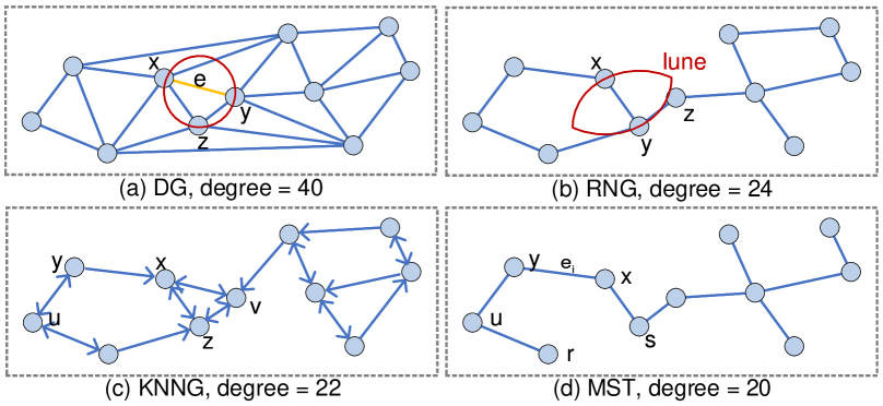
Figure 2. Schematic diagram of different base graphs’ construction results on the same dataset with dimension $d=2$.

Delaunay Graph (DG). In Euclidean space $E^{d}$, the DG $G(V,E)$ constructed on dataset $S$ satisfies the following conditions: For $\forall e\in E$ (e.g., the yellow line in Figure 2(a)), where its corresponding two vertices are ${x}$, ${y}$, there exists a circle (the red circle in Figure 2(a)) passing through ${x}$, ${y}$, and no other vertices inside the circle, and there are at most three vertices (i.e., ${x},{y},{z}$) on the circle at the same time (see (Fortune, 1995) for DG’s standard definition). DG ensures that the ANNS always return precise results (Malkov and Yashunin, 2018), but the disadvantage is that DG is almost fully connected when the dimension $d$ is extremely high, which leads to a large search space (Harwood and Drummond, 2016; Fu et al., 2019).

Relative Neighborhood Graph (RNG). In Euclidean space $E^{d}$, the RNG $G(V,E)$ built on dataset $S$ has the following property: For ${x},{y}\in V$, if ${x}$ and ${y}$ are connected by edge $e\in E$, then $\forall{z}\in V$, with $\delta({x},{y})<\delta({x},{z})$, or $\delta({x},{y})<\delta({z},{y})$. In other words, ${z}$ is not in the red lune in Figure 2(b) (for RNG’s standard definition, refer to (Toussaint, 1980)). Compared with DG, RNG cuts off some redundant neighbors (close to each other) that violate its aforementioned property, and makes the remaining neighbors distribute omnidirectionally, thereby reducing ANNS’ distance calculations (Malkov and Yashunin, 2018). However, the time complexity of constructing RNG on $S$ is $O(|S|^{3})$ (Jaromczyk and Kowaluk, 1991).

K-Nearest Neighbor Graph (KNNG). Each point in dataset $S$ is connected to its nearest $K$ points to form a KNNG $G(V,E)$ in Euclidean space $E^{d}$. As Figure 2(c) ($K=2$) shows, for ${x},{y}\in V$, ${x}\in N({y})=\left\{{x},{u}\right\}$, but ${y}\not\in N({x})=\left\{{z},{v}\right\}$, where $N({y}),N({x})$ are the neighbor sets of ${y}$ and ${x}$, respectively. Therefore, the edge between $y$ and $x$ is a directed edge, so KNNG is a directed graph. KNNG limits the number of neighbors of each vertex to $K$ at most, thus avoiding the surge of neighbors, which works well in scenarios with limited memory and high demand for efficiency. It can be seen that KNNG does not guarantee global connectivity in Figure 2(c), which is unfavorable for ANNS.

Minimum Spanning Tree (MST). In Euclidean space $E^{d}$, MST is the $G(V,E)$ with the smallest $\sum_{i=1}^{|E|}w(e_{i})$ on dataset $S$, where the two vertices associated with $e_{i}\in E$ are ${x}$ and ${y}$, $w(e_{i})=\delta({x},{y})$. If $\exists e_{i},e_{j}\in E$, $w(e_{i})=w(e_{j})$, then MST is not unique (Mathieson and Moscato, 2019). Although MST has not been adopted by most current graph-based ANNS algorithms, HCNNG (Munoz et al., 2019) confirms MST’s effectiveness as a neighbor selection strategy for ANNS. The main advantage for using MST as a base graph relies on the fact that MST uses the least edges to ensure the graph’s global connectivity, so that keeping vertices with low degrees and any two vertices are reachable. However, because of a lack of shortcuts, it may detour when searching on MST (Malkov et al., 2014; Fu et al., 2019). For example, in Figure 2(d), when search goes from $s$ to $r$, it must detour with ${s}\rightarrow{x}\rightarrow{y}\rightarrow{u}\rightarrow{r}$. This can be avoided if there is an edge between $s$ and $r$.

3.2. Graph-Based ANNS Algorithms

Table 2. Summary of important representative graph-based ANNS algorithms

Algorithm	Base Graph	Edge	Build Complexity	Search Complexity
KGraph (Dong, 2011)	KNNG	directed	$O(|S|^{1.14})$	$O(|S|^{0.54})$$\ddagger$
NGT (Iwasaki, 2015)	KNNG+DG+RNG	directed	$O(|S|^{1.14})$$\ddagger$	$O(|S|^{0.59})$$\ddagger$
SPTAG (Chen et al., 2018)	KNNG+RNG	directed	$O(|S|\cdot\log(|S|^{c}+t^{t}))$$\dagger$	$O(|S|^{0.68})$$\ddagger$
NSW (Malkov et al., 2014)	DG	undirected	$O(|S|\cdot\log^{2}(|S|))$$\ddagger$	$O(\log^{2}(|S|))^{\dagger}$
IEH (Jin et al., 2014)	KNNG	directed	$O(|S|^{2}\cdot\log(|S|)+|S|^{2})$$\ddagger$	$O(|S|^{0.52})$$\ddagger$
FANNG (Harwood and Drummond, 2016)	RNG	directed	$O(|S|^{2}\cdot\log(|S|))$	$O(|S|^{0.2})$
HNSW (Malkov and Yashunin, 2018)	DG+RNG	directed	$O(|S|\cdot\log(|S|))$	$O(\log(|S|))$
EFANNA (Fu and Cai, 2016)	KNNG	directed	$O(|S|^{1.13})$$\ddagger$	$O(|S|^{0.55})$$\ddagger$
DPG (Li et al., 2019)	KNNG+RNG	undirected	$O(|S|^{1.14}+|S|)$$\ddagger$	$O(|S|^{0.28})$$\ddagger$
NSG (Fu et al., 2019)	KNNG+RNG	directed	$O(|S|^{\frac{1+c}{c}}\cdot\log(|S|)+|S|^{1.14})$$\dagger$	$O(\log(|S|))$
HCNNG (Munoz et al., 2019)	MST	directed	$O(|S|\cdot\log(|S|))$	$O(|S|^{0.4})$$\ddagger$
Vamana (Subramanya et al., 2019)	RNG	directed	$O(|S|^{1.16}$)$\ddagger$	$O(|S|^{0.75}$)$\ddagger$
NSSG (Fu et al., 2021)	KNNG+RNG	directed	$O(|S|+|S|^{1.14})$	$O(\log(|S|))$

^† $c$, $t$ are the constants. ^‡ Complexity is not informed by the authors; we derive it based on the related papers’ descriptions and experimental estimates. See Appendix D for deatils.

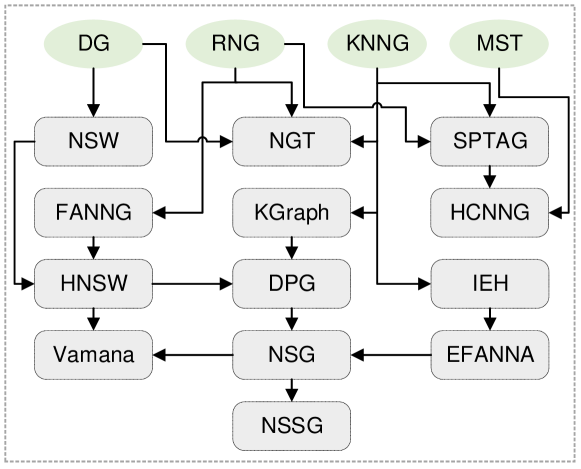
Figure 3. Roadmaps of graph-based ANNS algorithms. The arrows from a base graph (green shading) to an algorithm (gray shading) and from one algorithm to another indicate the dependence and development relationships.

Although the formal definition of base graphs facilitates theoretical analysis, it is impractical for them to be applied directly to ANNS (Fu et al., 2019). Obviously, their high construction complexity is difficult to scale to large-scale datasets. This has become even truer with the advent of frequently updated databases (Li et al., 2018). In addition, it is difficult for base graphs to achieve high search efficiency in high-dimensional scenarios (Harwood and Drummond, 2016; Fu et al., 2019; Ponomarenko et al., 2014). Thus, a number of graph-based ANNS algorithms tackle improving the base graphs from one or several aspects. Next, we outline 13 representative graph-based ANNS algorithms (A1–A13) based on the aforementioned four base graphs and their development roadmaps (Figure 3). Table 2 summarizes some important properties about algorithms.

DG-based and RNG-based ANNS algorithms (NSW, HNSW, FANNG, NGT). To address the high degree of DG in high dimension, some slight improvements have been proposed (Kleinberg, 2000; Beaumont et al., 2007b; Beaumont et al., 2007a). However, they rely heavily on DG’s quality and exist the curse of dimensionality (Malkov et al., 2014). Therefore, some algorithms add an RNG approximation on DG to diversify the distribution of neighbors (Malkov and Yashunin, 2018).

A1: Navigable Small World graph (NSW). NSW (Malkov et al., 2014) constructs an undirected graph through continuous insertion of elements and ensures global connectivity (approximate DG). The intuition is that the result of a greedy traversal (random seeds) is always the nearest neighbor on DG (Malkov and Yashunin, 2018). The long edges formed in the beginning of construction have small-world navigation performance to ensure search efficiency, and the vertices inserted later form short-range edges, which ensure search accuracy. NSW also achieved excellent results in the maximum inner product search (Morozov and Babenko, 2018; Liu et al., 2020). However, according to the evaluation of (Ponomarenko et al., 2014), NSW provides limited best tradeoffs between efficiency and effectiveness compared to non-graph-based indexes, because its search complexity is poly-logarithmic (Naidan et al., 2015). In addition, NSW uses undirected edges to connect vertices, which results in vertices in dense areas acting as the “traffic hubs” (high out-degrees), thus damaging search efficiency.

A2: Hierarchical Navigable Small World graphs (HNSW). An improvement direction is put forth by (Malkov and Ponomarenko, 2016; Boguna et al., 2009) to overcome NSW’s poly-logarithmic search complexity. Motivated by this, HNSW (Malkov and Yashunin, 2018) generates a hierarchical graph and fixes the upper bound of each vertex’s number of neighbors, thereby allowing a logarithmic complexity scaling of search. Its basic idea is to separate neighbors to different levels according to the distance scale, and the search is an iterative process from top to bottom. For an inserted point, HNSW not only selects its nearest neighbors (approximate DG), but also considers the distribution of neighbors (approximate RNG). HNSW has been deployed in various applications (Boytsov et al., 2016; Kosuge and Oshima, 2019; Bee et al., 2020) because of its unprecedented superiority. However, its multilayer structure significantly increases the memory usage and makes it difficult to scale to larger datasets (Fu et al., 2019). Meawhile, (Lin and Zhao, 2019) experimentally verifies that the hierarchy’s advantage fades away as intrinsic dimension goes up (¿32). Hence, recent works try to optimize HNSW by hardware or heterogeneous implementation to alleviate these problems (Zhang and He, 2019; Deng et al., 2019).

A3: Fast Approximate Nearest Neighbor Graph (FANNG). An occlusion rule is proposed by FANNG (Harwood and Drummond, 2016) to cut off redundant neighbors (approximate RNG). Unlike HNSW’s approximation to RNG (HNSW only considers a small number of vertices returned by greedy search), FANNG’s occlusion rule is applied to all other points on the dataset except the target point, which leads to high construction complexity. Thus, two intuitive optimizations of candidate neighbor acquisition are proposed to alleviate this problem (Harwood and Drummond, 2016). To improve the accuracy, FANNG uses backtrack to the second-closest vertex and considers its edges that have not been explored yet.

A4: Neighborhood Graph and Tree (NGT). NGT (Iwasaki, 2015) is a library for performing high-speed ANNS released by Yahoo Japan Corporation. It contains two construction methods. One is to transform KNNG into Bi-directed KNNG (BKNNG), which adds reverse edges to each directed edge on KNNG (Iwasaki, 2016). The other is constructed incrementally like NSW (approximate to DG) (Iwasaki, 2016). The difference from NSW is range search (a variant of greedy search) used during construction. Both of the aforementioned methods make certain hub vertices have a high out-degree, which will seriously affect search efficiency. Therefore, NGT uses three degree-adjustment methods to alleviate this problem, and within the more effective path adjustment is an approximation to RNG (see Appendix B for proof) (Iwasaki and Miyazaki, 2018). This reduces memory overhead and improves search efficiency. NGT obtains the seed vertex through the VP-tree (Iwasaki and Miyazaki, 2018), and then uses the range search to perform routing. Interestingly, the NGT-like path adjustment and range search are also used by the k-DR algorithm in (Aoyama et al., 2011) (see Appendix N for details).

KNNG-based ANNS algorithms (SPTAG, KGraph, EFANNA, IEH). A naive construction for KNNG is exhaustively comparing all pairs of points, which is prohibitively slow and unsuitable for large dataset $S$. Some early solutions construct an additional index (such as tree (Paredes et al., 2006) or hash (Uno et al., 2009; Zhang et al., 2013)), and then find the neighbors of each point through ANNS. However, such methods generally suffer from high index construction complexity (Chen et al., 2009). This is because they ignore this fact: the queries belong to $S$ in the graph construction process, but the queries of ANNS generally do not (Wang et al., 2012). Thus, it is unnecessary to ensure a good result is given for general queries on additional index (Wang et al., 2012). There are two types of representative solutions, which only focus on graph construction.

A5: Space Partition Tree and Graph (SPTAG). One is based on divide and conquer, and its representative is SPTAG (Chen et al., 2018), a library released by Microsoft. SPTAG hierarchically divides dataset $S$ into subsets (through Trinary-Projection Trees (Wang et al., 2013b)) and builds an exact KNNG over each subset. This process repeats multiple times to produce a more accurate KNNG on $S$. Moreover, SPTAG further improves KNNG’s accuracy by performing neighborhood propagation (Wang et al., 2012). The early version of SPTAG added multiple KD-trees on $S$ to iteratively obtain the seeds closer to the query (Wang and Li, 2012). However, on extremely high-dimensional $S$, the KD-trees will produce an inaccurate distance bound estimation. In response, the balanced k-means trees are constructed to replace the KD-trees (Chen et al., 2018). Inspired by the universal superiority brought about by RNG, SPTAG has recently added the option of approximating RNG in the project (Chen et al., 2018).

A6: KGraph. The other is based on NN-Descent (Dong et al., 2011); its basic idea is neighbors are more likely to be neighbors of each other (Fu and Cai, 2016). KGraph (Dong, 2011) first adopts this idea to reduce KNNG’s construction complexity to $O(|S|^{1.14})$ on dataset $S$. It achieves better search performance than NSW (Bernhardsson, 2017). Therefore, some NN-Descent-based derivatives are developed to explore its potential (Bratić et al., 2018; Zhao et al., 2019a; Zhao, 2018).

A7: EFANNA and A8: IEH. Instead of random initialization during construction (such as KGraph), Extremely Fast Approximate Nearest Neighbor Search Algorithm (EFANNA) (Fu and Cai, 2016) first builds multiple KD-trees on $S$, and better initializes the neighbors of each vertex through ANNS on these KD-trees, then executes NN-Descent. At the search stage, EFANNA also uses these KD-trees to obtain seeds that are closer to the query. The idea of initializing seeds through additional structures is inspired by Iterative Expanding Hashing (IEH) (Jin et al., 2014), which uses hash buckets to obtain better seeds. However, IEH’s KNNG is constructed by brute force in (Jin et al., 2014).

KNNG-based and RNG-based ANNS algorithms (DPG, NSG, NSSG, Vamana). The early optimization of KGraph was limited to improving graph quality (Fu and Cai, 2016; Zhao, 2018). Their intuition is that higher graph quality leads to better search performance. Hence, each vertex is only connected to $K$ nearest neighbors without considering the distribution of neighbors. According to the comparative analysis of (Lin and Zhao, 2019), if neighbors of a visiting vertex are close to each other, it will guide the search to the same location. That is, it is redundant to compare the query to all neighbors close to each other (Harwood and Drummond, 2016; Malkov and Yashunin, 2018).

A9: Diversified Proximity Graph (DPG). To overcome the aforementioned issue, DPG (Li et al., 2019) practices optimization to control neighbors’ distribution on KGraph. It sets the threshold of the angle between the neighbors of a vertex to make the neighbors evenly distributed in all directions of the vertex. This is only an approximate implementation of RNG from another aspect (see Appendix C for the proof). In addition, to deal with $S$ with a large number of clusters, DPG keeps bi-directed edges on the graph.

A10: Navigating Spreading-out Graph (NSG). Although DPG’s search performance is comparable to HNSW, it suffers from a large index (Fu et al., 2019). To settle this problem and further improve search performance, NSG (Fu et al., 2019) proposes an edge selection strategy based on monotonic RNG (called MRNG), which is actually equivalent to HNSW’s (see Appendix A for the proof). Its construction framework is inspired by DPG; that is, to prune edges on KNNG. NSG ensures high construction efficiency by executing ANNS on KGraph to obtain candidate neighbors. NSG has been integrated into Alibaba’s Taobao e-commerce platform to combine superior index construction and search performance (Fu et al., 2019), and its billion-scale implementation version exceeds the current best FAISS (Johnson et al., 2017).

A11: Navigating Satellite System Graph (NSSG). NSSG continues to explore the potential of pruning edges on KNNG, and proposes an edge selection strategy based on SSG (Fu et al., 2021). When obtaining a vertex’s candidate neighbors, instead of conducting the ANNS like NSG, it gets the neighbors and neighbors’ neighbors of the vertex on KNNG, which significantly improves construction efficiency. Both SSG and MRNG are approximations to RNG, but SSG is relatively relaxed when cutting redundant neighbors. Therefore, NSSG has a larger out-degree. Although (Fu et al., 2021) believes that SSG is more beneficial to ANNS than MRNG, we reach the opposite conclusion through a fairer evaluation (see §5.4 for details).

A12: Vamana. Microsoft recently proposed Vamana (Subramanya et al., 2019) to combine with solid-state drives (SSD) for billions of data. It analyzes the construction details of HNSW and NSG to extract and combine the better parts. Its construction framework is motivated by NSG. Instead of using KGraph to initialize like NSG, Vamana initializes randomly. When selecting neighbors, Vamana improves the HNSW’s strategy by adding a parameter $\alpha$ to increase the edge selection’s flexibility and executing two passes with different $\alpha$. Experiments show that its result graph has a shorter average path length when searching, which works well with SSD.

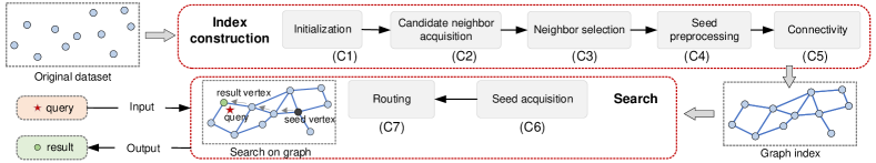
Figure 4. The pipeline of graph-based ANNS algorithms. An algorithm can be divided into two coarse-grained components: index construction, search. We subdivide the index construction into five fine-grained components (C1–C5), the search into two fine-grained components (C6–C7).

MST-based ANNS algorithms (HCNNG).

A13: HCNNG. Different from the aforementioned techniques, a recent method called Hierarchical Clustering-based Nearest Neighbor Graph (HCNNG) (Munoz et al., 2019) uses MST to connect the points on dataset $S$. It uses the same divide-and-conquer framework as SPTAG. The difference is that HCNNG divides $S$ through multiple hierarchical clusters, and all points in each cluster are connected through MST. HCNNG uses multiple global KD-trees to get seeds (like SPTAG and EFANNA). Then to improve search efficiency, rather than using traditional greedy search, it performs an efficient guided search.

4. Components’ Analysis

Despite the diversity of graph-based ANNS algorithms, they all follow a unified processing pipeline. As Figure 4 shows, an algorithm can be divided into two coarse-grained components: index construction (top) and search (bottom), which are adopted by most of the current work to analyze algorithms (Malkov et al., 2014; Li et al., 2019; Harwood and Drummond, 2016; Munoz et al., 2019). Recent research has endeavored to take a deeper look at some fine-grained components (Fu et al., 2019; Fu et al., 2021), prompting them to find out which part of an algorithm plays a core role and then propose better algorithms. Motivated by this, we subdivide the index construction and search into seven fine-grained components (C1–C7 in Figure 4), and compare all 13 graph-based algorithms discussed in this paper by them.

4.1. Components for Index Construction

The purpose of index construction is to organize the dataset $S$ with a graph. Existing algorithms are generally divided into three strategies: Divide-and-conquer (Virmajoki and Franti, 2004), Refinement (Dong et al., 2011), and Increment (Hajebi et al., 2011) (see Appendix E). As Figure 4 (top) show, an algorithm’s index construction can be divided into five detailed components (C1–C5). Among them, initialization can be divided into three ways according to different construction strategies.

C1: Initialization.

Overview. The initialization of Divide-and-conquer is dataset division; it is conducted recursively to generate many subgraphs so that the index is obtained by subgraph merging (Shimomura and Kaster, 2019; Chen et al., 2009). For Refinement, in the initialization, it performs neighbor initialization to get the initialized graph, then refines the initialized graph to achieve better search performance (Fu and Cai, 2016; Fu et al., 2019). While the Increment inserts points continuously, the new incoming point is regarded as a query, then it executes ANNS to obtain the query’s neighbors on the subgraph constructed by the previously inserted points (Malkov et al., 2014; Malkov and Yashunin, 2018); it therefore implements seed acquisition during initialization.

Definition 4.1.

Dataset Division. Given dataset $S$, the dataset division divides $S$ into $m$ small subsets—i.e., $S_{0},S_{1},\cdots,S_{m-1}$, and $S_{0}\cup S_{1}\cdots\cup S_{m-1}=S$.

Data division. This is a unique initialization of the Divide-and-conquer strategy. SPTAG previously adopts a random division scheme, which generates the principal directions over points randomly sampled from $S$, then performs random divisions to make each subset’s diameter small enough (Verma et al., 2009; Wang et al., 2012). To achieve better division, SPTAG turns to TP-tree (Wang et al., 2013b), in which a partition hyperplane is formed by a linear combination of a few coordinate axes with weights being -1 or 1. HCNNG divides $S$ by iteratively performing hierarchical clustering. Specifically, it randomly takes two points from the set to be divided each time, and performs division by calculating the distance between other points and the two (Munoz et al., 2019).

Definition 4.2.

Neighbor Initialization. Given dataset $S$, for $\forall p\in S$, the neighbor initialization gets the subset $C$ from $S\setminus\left\{p\right\}$, and initializes $N(p)$ with $C$.

Neighbor initialization. Only the initialization of the Refinement strategy requires this implementation. Both KGraph and Vamana implement this process by randomly selecting neighbors (Dong, 2011; Subramanya et al., 2019). This method offers high efficiency but the initial graph quality is too low. The solution is to initialize neighbors through ANNS based on hash-based (Uno et al., 2009) or tree-based (Fu and Cai, 2016) approaches. EFANNA deploys the latter; it establishes multiple KD-trees on $S$. Then, each point is treated as a query, and get its neighbors through ANNS on multiple KD-trees (Fu and Cai, 2016). This approach relies heavily on extra index and increases the cost of index construction. Thus, NSG, DPG, and NSSG deploy the NN-Descent (Dong et al., 2011); they first randomly select neighbors for each point, and then update each point’s neighbors with neighborhood propagation. Finally, they get a high-quality initial graph by a small number of iterations. Specially, FANNG and IEH initialize neighbors via linear scan.

Definition 4.3.

Seed Acquisition. Given the index $G(V,E)$, the seed acquisition acquires a small subset $\widehat{S}$ from $V$ as the seed set, and ANNS on $G$ starts from $\widehat{S}$.

Seed acquisition. The seed acquisition of the index construction is Increment strategy’s initialization. The other two strategies may also include this process when acquiring candidate neighbors, and this process also is necessary for all graph-based algorithms in the search. For index construction, both NSW and NGT obtain seeds randomly (Malkov et al., 2014; Iwasaki, 2015), while HNSW makes its seed points fixed from the top layer because of its unique hierarchical structure (Malkov and Yashunin, 2018).

Definition 4.4.

Candidate Neighbor Acquisition. Given a finite dataset $S$, point $p\in S$, the candidate neighbor acquisition gets a subset $\mathcal{C}$ from $S\setminus\left\{p\right\}$ as $p$’s candidate neighbors, and $p$ get its neighbors $N(p)$ from $\mathcal{C}$—that is, $N(p)\subset\mathcal{C}$.

C2: Candidate neighbor acquisition. The graph constructed by the Divide-and-conquer generally produce candidate neighbors from a small subset obtained after dataset division. For a subset $S_{i}\subset S$ and a point $p\in S_{i}$, SPTAG and HCNNG directly take $S_{i}\setminus\left\{p\right\}$ as candidate neighbors (Wang et al., 2012; Munoz et al., 2019). Although $|S|$ may be large, the $|S_{i}|$ obtained by the division is generally small. However, Refinement and Increment do not involve the process of dataset division, which leads to low index construction efficiency for IEH and FANNG to adopt the naive method of obtaining candidate neighbors (Jin et al., 2014; Harwood and Drummond, 2016). To solve this problem, NGT, NSW, HNSW, NSG, and Vamana all obtain candidate neighbors through ANNS. For a point $p\in S$, the graph $G_{sub}$ (Increment) formed by the previously inserted points or the initialized graph $G_{init}$ (Refinement), they consider $p$ as a query and execute ANNS on $G_{sub}$ or $G_{init}$, and finally return the query result as candidate neighbors of $p$. This method only needs to access a small subset of $S$. However, according to the analysis of (Wang et al., 2012), obtaining candidate neighbors through ANNS is overkill, because the query is in $S$ for index construction, but the ANNS query generally does not belong to $S$. In contrast, KGraph, EFANNA, and NSSG use the neighbors of $p$ and neighbors’ neighbors on $G_{init}$ as its candidate neighbors (Fu et al., 2021), which improves index-construction efficiency. DPG directly uses the neighbors of $p$ on $G_{init}$ as candidate neighbors, but to obtain enough candidate neighbors, it generally requires $G_{init}$ with a larger out-degree (Li et al., 2019).

Definition 4.5.

Neighbor Selection. Given a point $p$ and its candidate neighbors $\mathcal{C}$, the neighbor selection obtains a subset of $\mathcal{C}$ to update $N(p)$.

C3: Neighbor selection. The current graph-based ANNS algorithms mainly consider two factors for this component: distance and space distribution. Given $p\in S$, the distance factor ensures that the selected neighbors are as close as possible to $p$, while the space distribution factor makes the neighbors distribute as evenly as possible in all directions of $p$. NSW, SPTAG, NGT¹, KGraph, EFANNA, and IEH only consider the distance factor and aim to build a high-quality graph index (Wang et al., 2012; Dong et al., 2011). HNSW, FANNG, SPTAG, and NSG² consider the space distribution factor by evaluating the distance between neighbors, formally, for $x\in\mathcal{C}$, $\forall y\in N(p)$, iff $\delta(x,y)>\delta(y,p)$, $x$ will join $N(p)$ (Harwood and Drummond, 2016; Fu et al., 2019). To select neighbors more flexibly, Vamana adds the parameter $\alpha$ so that for $x\in\mathcal{C}$, $\forall y\in N(p)$, iff $\alpha\cdot\delta(x,y)>\delta(y,p),(\alpha\geq 1)$, $x$ will be added to $N(p)$ (Subramanya et al., 2019), so it can control the distribution of neighbors well by adjusting $\alpha$. DPG obtains a subset of $\mathcal{C}$ to minimize the sum of angles between any two points, thereby dispersing the neighbor distribution (Li et al., 2019). NSSG considers the space distribution factor by setting an angle threshold $\theta$, for $x\in\mathcal{C}$, $\forall y\in N(p)$, iff $\arccos(x,y)<\theta$, $x$ will join $N(p)$. NGT³ indirectly attains the even distribution of neighbors with path adjustment (Iwasaki and Miyazaki, 2018), which updates neighbors by judging whether there is an alternative path between point $p$ and its neighbors on $G_{init}$. HCNNG selects neighbors for $p$ by constructing an MST on $\left\{p\right\}\cup\mathcal{C}$ (Munoz et al., 2019). Recently, (Zhang et al., 2019; Baranchuk and Babenko, 2019) perform neighbor selection through learning, but these methods are difficult to apply in practice because of their extremely high training costs.

C4: Seed preprocessing. Different algorithms may exist with different execution sequences between this component and the connectivity, such as NSW (Malkov et al., 2014), NSG (Fu et al., 2019). Generally, graph-based ANNS algorithms implement this component in a static or dynamic manner. For the static method, typical representatives are HNSW, NSG, Vamana, and NSSG. HNSW fixes the top vertices as the seeds, NSG and Vamana use the approximate centroid of $S$ as the seed, and the seeds of NSSG are randomly selected vertices. While for the dynamic method, a common practice is to attach other indexes (i.e., for each query, the seeds close to the query are obtained through an additional index). SPTAG, EFANNA, HCNNG, and NGT build additional trees, such as KD-tree (Fu and Cai, 2016; Chen et al., 2018), balanced k-means tree (Chen et al., 2018), and VP-tree (Iwasaki, 2015). IEH prepares for seed acquisition through hashing (Jin et al., 2014). Then (Douze et al., 2018) compresses the original vector by OPQ  (Ge et al., 2013) to obtain the seeds by quickly calculating the compressed vector. Random seed acquisition is adopted by KGraph, FANNG, NSW, and DPG, and they don’t need to implement seed preprocessing.

C5: Connectivity. Incremental strategy internally ensures connectivity (e.g., NSW). Refinement generally attaches depth-first traversal to achieve this (Fu et al., 2019) (e.g., NSG). Divide-and-conquer generally ensures connectivity by multiply performing dataset division and subgraph construction (e.g., SPTAG).

4.2. Components for Search

We subdivide the search into two fine-grained components (C6–C7): seed acquisition and routing.

C6: Seed acquisition. Because the seed has a significant impact on search, this component of the search process is more concerned than the initialization of Incremental strategy. Some early algorithms obtain the seeds randomly, while state-of-the-art algorithms commonly use seed preprocessing. If the fixed seeds are produced in the preprocessing stage, it can be loaded directly at this component. If other index structures are constructed in the preprocessing stage, ANNS returns the seeds with the additional structure.

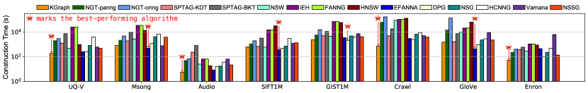
Figure 5. Index construction time of all compared algorithms on real-world datasets (the bar marked with a red star is the best).

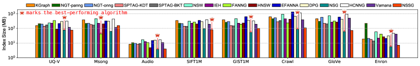
Figure 6. Index size of all compared algorithms on real-world datasets (the bar marked with a red star is the best).

Definition 4.6.

Routing. Given $G(V,E)$, query $q$, seed set $\widehat{S}$, the routing starts from the vertices in $\widehat{S}$, and then converges to $q$ by neighbor propagation along the neighbor $n$ of the visited point with smaller $\delta(n,q)$, until the vertex $r$ so that $\delta(r,q)$ reaches a minimum.

Definition 4.7.

Best First Search. Given $G(V,E)$, query $q$, and vertices to be visited $\mathcal{C}$, its maximum size is $c$ and the result set $\mathcal{R}$. We initialize $\mathcal{C}$ and $\mathcal{R}$ with seed set $\widehat{S}$. For $\hat{x}=\arg\,\min_{x\in\mathcal{C}}{\delta(x,q)}$, best first search access $N(\hat{x})$, then $\mathcal{C}\setminus\left\{\hat{x}\right\}$ and $\mathcal{C}\cup N(\hat{x})$. To keep $|\mathcal{C}|=c$, $\hat{y}=\arg\,\max_{y\in\mathcal{C}}{\delta(y,q)}$ will be deleted. $\forall n\in N(\hat{x})$, if $\delta(n,q)<\delta(\hat{z},q),\hat{z}=\arg\,\max_{z\in\mathcal{R}}{\delta(z,q)}$, then $\mathcal{R}\setminus\left\{\hat{z}\right\}$ and $\mathcal{R}\cup\left\{n\right\}$. The aforementioned process is performed iteratively until $\mathcal{R}$ is no longer updated. (see Appendix F for the pseudocode)

C7: Routing. Almost all graph-based ANNS algorithms are based on a greedy routing strategy, including best first search (BFS) and its variants. NSW, HNSW, KGraph, IEH, EFANNA, DPG, NSG, NSSG, and Vamana use the original BFS to perform routing. Despite this method being convenient for deployment, it has two shortcomings: susceptibility to local optimum (S1) (Baranchuk et al., 2019) and low routing efficiency (S2) (Munoz et al., 2019). S1 destroys the search results’ accuracy. For this problem, FANNG adds backtracking to BFS, which slightly improves the search accuracy while significantly increasing the search time (Harwood and Drummond, 2016). NGT alleviates S1 by adding a parameter $\epsilon$. On the basis of Definition 4.7, it cancels the size restriction on $\mathcal{C}$ and takes $\delta(\hat{y},q)$ as the search radius $r$, for $\forall n\in N(\hat{x})$, if $\delta(n,q)<(1+\epsilon)\cdot r$, then $n$ is added to $\mathcal{C}$. Setting $\epsilon$ to a larger value can alleviate S1, but it will also significantly increase the search time (Iwasaki and Miyazaki, 2018). SPTAG solves S1 by iteratively executing BFS. When a certain iteration falls into a local optimum, it will restart the search by selecting new seeds from the KD-tree (Wang and Li, 2012). HCNNG proposes using guided search to alleviate S2 rather than visiting all $N(\hat{x})$ like BFS, so guided search avoids some redundant visits based on the query’s location. Recently, some of the literature uses learning methods to perform routing (Baranchuk et al., 2019; Li et al., 2020; Vargas Muñoz et al., 2019). These methods usually alleviate S1 and S2 simultaneously, but the adverse effect is that this requires extra training, and additional information also increases the memory overhead (see §5.5).

5. Experimental Evaluation

This section presents an abundant experimental study of both individual algorithms (§3) and components (§4) extracted from the algorithms for graph-based ANNS. Because of space constraints, some of our experimental content is provided in appendix. Our evaluation seeks to answer the following question:

Q1: How do the algorithms perform in different scenarios? (§5.2–5.3)

Q2: Can an algorithm have the best index construction and search performance at the same time? (§5.2–5.3)

Q3: For an algorithm with the best overall performance, is the performance of each fine-grained component also the best? (§5.4)

Q4: How do machine learning-based optimizations affect the performance of the graph-based algorithms? (§5.5)

Q5: How can we design a better graph-based algorithm based on the experimental observations and verify its performance? (§6)

5.1. Experimental Setting

Datasets. Our experiment involves eight real-world datasets popularly deployed by existing works, which cover various applications such as video (UQ-V (Anon, nownc)), audio (Msong (Anon, 2011), Audio (Anon, nownb)), text (Crawl (Anon, nowna), GloVe (Jeffrey et al., 2015), Enron (Russell et al., 2015)), and image (SIFT1M (Anon, 2010), GIST1M (Anon, 2010)). Their main characteristics are summarized in Table 3. # Base is the number of elements in the base dataset. LID indicates local intrinsic dimensionality, and a larger LID value implies a “harder” dataset (Li et al., 2019). Additionally, 12 synthetic datasets are used to test each algorithm’s scalability to different datasets’ performance (e.g., dimensionality, cardinality, number of clusters, and standard deviation of the distribution in each cluster (Shimomura et al., 2020)). Out of space considerations, please see the scalability evaluation in Appendix J. All datasets in the experiment are processed into the base dataset, query dataset, and ground-truth dataset.

Table 3. Statistics of real-world datasets.

Dataset	Dimension	# Base	# Query	LID (Li et al., 2019; Fu et al., 2021)
UQ-V (Anon, nownc)	256	1,000,000	10,000	7.2
Msong (Anon, 2011)	420	992,272	200	9.5
Audio (Anon, nownb)	192	53,387	200	5.6
SIFT1M (Anon, 2010)	128	1,000,000	10,000	9.3
GIST1M (Anon, 2010)	960	1,000,000	1,000	18.9
Crawl (Anon, nowna)	300	1,989,995	10,000	15.7
GloVe (Jeffrey et al., 2015)	100	1,183,514	10,000	20.0
Enron (Russell et al., 2015)	1,369	94,987	200	11.7

Compared algorithms. Our experiment evaluates 13 representative graph-based ANNS algorithms mentioned in §3, which are carefully selected from research literature and practical projects. The main attributes and experimental parameters of these algorithms are introduced in Appendix E and Appendix F.

Evaluation metrics. To measure the algorithm’s overall performance, we employ various metrics related to index construction and search. For index construction, we evaluate the index construction efficiency and size. Some index characteristics such as graph quality, average out-degree, and the number of connected components are recorded; they indirectly affect index construction efficiency and size. Given a proximity graph $G^{\prime}(V^{\prime},E^{\prime})$ (graph index of an algorithm) and the exact graph $G(V,E)$ on the same dataset, we define graph quality of an index as $\frac{|E^{\prime}\bigcap E|}{|E|}$ (Wang et al., 2013a; Chen et al., 2009; Boutet et al., 2016). For search, we evaluate search efficiency, accuracy, and memory overhead. Search efficiency can be measured by queries per second (QPS) and speedup. QPS is the ratio of the number of queries ($\#q$) to the search time ($t$); i.e., $\frac{\#q}{t}$ (Fu et al., 2019). Speedup is defined as $\frac{|S|}{NDC}$, where $|S|$ is the dataset’s size and is also the number of distance calculations of the linear scan for a query, and $NDC$ is the number of distance calculations of an algorithm for a query (equal to $|\mathcal{C}|$ in Definition 2.2) (Munoz et al., 2019). We use the recall rate to evaluate the search accuracy, which is defined as $\frac{|R\cup T|}{|T|}$, where $R$ is an algorithm’s query result set, $T$ is the real result set, and $|R|=|T|$. We also measure other indicators that indirectly reflect search performance, such as the candidate set size during the search and the average query path length.

Implementation setup. We reimplement all algorithms by C++; they were removed by all the SIMD, pre-fetching instructions, and other hardware-specific optimizations. To improve construction efficiency, the parts involving vector calculation are parallelized for index construction of each algorithm (Tellez et al., 2021; Aumüller and Ceccarello, 2019). All C++ source codes are compiled by g++ 7.3, and MATLAB source codes (only for index construction of a hash table in IEH (Jin et al., 2014)) are compiled by MATLAB 9.9. All experiments are conducted on a Linux server with a Intel(R) Xeon(R) Gold 5218 CPU at 2.30GHz, and a 125G memory.

Parameters. Because parameters’ adjustment in the entire base dataset may cause overfitting (Fu et al., 2019), we randomly sample a certain percentage of data points from the base dataset to form a validation dataset. We search for the optimal value of all the adjustable parameters of each algorithm on each validation dataset, to make the algorithms’ search performance reach the optimal level. Note that high recall areas’ search performance primarily is concerned with the needs of real scenarios.

5.2. Index Construction Evaluation

We build indexes of all compared algorithms in 32 threads on each real-world dataset. Note that we construct each algorithm with the parameters under optimal search performance.

Construction efficiency. The construction efficiency is mainly affected by the construction strategy, algorithm category, and dataset. In Figure 5, the KNNG-based algorithms (e.g., KGraph and EFANNA) constructed by NN-Descent have the smallest construction time among all test algorithms, while the KNNG-based algorithms constructed by divide and conquer (e.g., SPTAG) or brute force (e.g., IEH) have higher construction time. The construction time of RNG-based algorithms vary greatly according to the initial graph. For example, when adding the approximation of RNG on KGraph (e.g., DPG and NSSG), it has a high construction efficiency. However, RNG approximation based on the KNNG built by brute force (e.g., FANNG) has miniscule construction efficiency (close to IEH). Note that Vamana is an exception; its ranking on different datasets has large differences. This is most likely attributable to its neighbor selection parameter $\alpha$ heavily dependent on dataset. The construction time of DG-based algorithms (e.g., NGT and NSW) shows obvious differences with datasets. On some hard datasets (e.g., GloVe), their construction time is even higher than FANNG.

Index size and average out-degree. The index size mainly depends on the average out-degree (AD). Generally, the smaller the AD, the smaller the index size. As Figure 6 and Table 4 show, RNG-based algorithms (e.g., NSG) have a smaller index size, which is mainly because they cut redundant edges (the lower AD) during RNG approximation. KNNG-, DG-, and MST-based algorithms (e.g., KGraph, NSW, and HCNNG) connect all nearby neighbors without pruning superfluous neighbors, so they always have a larger index size. Additional index structures (e.g., the tree in NGT) will also increase related algorithms’ index size.

Graph quality. The algorithm category and dataset are the main factors that determine graph quality (GQ). In Table 4, the GQ of KNNG-based algorithms (e.g., KGraph) outperform other categories. The approximation to RNG prunes some of the nearest neighbors, thereby destroying RNG-based algorithms’ GQ (e.g., NSG). However, this phenomenon does not happen with DPG, mostly because it undirects all edges. Interestingly, DG- and MST-based algorithms’ GQ (e.g., NSW and HCNNG) shows obvious differences with datasets; on simple datasets (e.g., Audio), they have higher GQ, but it degrades on hard datasets (e.g., GIST1M).

Table 4. Graph quality (GQ), average out-degree (AD), and # of connected components (CC) on graph indexes (the bold values are the best).

Alg.	UQ-V			Msong			Audio			SIFT1M			GIST1M			Crawl			GloVe			Enron
	GQ	AD	CC	GQ	AD	CC	GQ	AD	CC	GQ	AD	CC	GQ	AD	CC	GQ	AD	CC	GQ	AD	CC	GQ	AD	CC
KGraph	0.974	40	8,840	1.000	100	3,086	0.994	40	529	0.998	90	331	0.995	100	39,772	0.927	80	290,314	0.949	100	183,837	0.992	50	3,743
NGT-panng	0.770	52	1	0.681	56	1	0.740	49	1	0.762	56	1	0.567	67	1	0.628	58	1	0.589	66	1	0.646	55	1
NGT-onng	0.431	47	1	0.393	55	1	0.412	45	1	0.424	53	1	0.266	75	1	0.203	66	1	0.220	124	1	0.331	53	1
SPTAG-KDT	0.957	32	27,232	0.884	32	110,306	0.999	32	996	0.906	32	23,132	0.803	32	290,953	0.821	32	672,566	0.630	32	594,209	0.983	32	7,500
SPTAG-BKT	0.901	32	71,719	0.907	32	42,410	0.992	32	61	0.763	32	82,336	0.435	32	45,9529	0.381	32	1,180,072	0.330	32	803,849	0.775	32	20,379
NSW	0.837	60	1	0.767	120	1	0.847	80	1	0.847	80	1	0.601	120	1	0.719	120	1	0.636	160	1	0.796	160	1
IEH	1.000	50	24,564	1.000	50	9,133	1.000	50	335	1.000	50	1,211	1.000	50	74,663	1.000	50	289,983	1.000	50	220,192	1.000	50	3,131
FANNG	1.000	90	3,703	0.559	10	15,375	1.000	50	164	0.999	70	256	0.998	50	47,467	0.999	30	287,098	1.000	70	175,610	1.000	110	1,339
HNSW	0.597	19	433	0.762	50	36	0.571	20	1	0.879	49	22	0.633	57	122	0.726	52	3,586	0.630	56	624	0.833	68	9
EFANNA	0.975	40	8,768	0.997	50	10,902	0.976	10	3,483	0.998	60	832	0.981	100	44,504	0.990	100	227,146	0.751	100	234,745	0.999	40	3,921
DPG	0.973	77	2	1.000	82	1	0.999	74	1	0.998	76	1	0.992	94	1	0.982	88	1	0.872	93	1	0.993	84	1
NSG	0.562	19	1	0.487	16	1	0.532	17	1	0.551	24	1	0.402	13	1	0.540	10	1	0.526	12	1	0.513	14	1
HCNNG	0.836	41	1	0.798	69	1	0.847	38	1	0.887	61	1	0.354	42	1	0.503	109	1	0.425	167	1	0.662	85	1
Vamana	0.034	30	5,982	0.009	30	2,952	0.185	50	1	0.021	50	82	0.016	50	209	0.020	50	730	0.024	110	3	0.234	110	1
NSSG	0.508	19	1	0.634	40	1	0.494	19	1	0.579	20	1	0.399	26	1	0.580	13	1	0.474	15	1	0.517	19	1

Connectivity. Connectivity mainly relates to the construction strategy and dataset. Table 4 shows that DG- and MST-based algorithms have good connectivity. The former is attributed to the Increment construction strategy (e.g., NSW and NGT), and the latter benefits from its approximation to MST. Some RNG-based algorithms perform depth-first search (DFS) to ensure connectivity (e.g., NSG and NSSG). DPG adds reverse edges to make it have good connectivity. Unsurprisingly, KNNG-based algorithms generally have a lot of connected components, especially on hard datasets.

5.3. Search Performance

All searches are evaluated on a single thread. The number of nearest neighbors recalled is uniformly set to 10 for each query, and $Recall@10$ represents the corresponding recall rate. Because of space constraints, we only list the representative results in Figure 7 and 8, and the others are displayed in Appendix O. Note that our observations are based on the results on all datasets.

Accuracy and efficiency. As illustrated in Figure 7 and 8, the search performance of different algorithms on the same dataset or the same algorithm on different datasets have large differences. Generally, algorithms capable of obtaining higher speedup also can achieve higher QPS, which demonstrates that the search efficiency of graph-based ANNS algorithms mainly depends on the number of distance evaluations during the search (Zhao et al., 2020). The search performance of RNG- and MST-based algorithms (e.g., NSG and HCNNG) generally beats other categories by a large margin, especially on hard datasets (e.g., GloVe). KNNG- and DG-based algorithms (e.g., EFANNA and NSW) can only achieve better search performance on simple datasets, their performance drops sharply on hard datasets. Particularly, the search performance of SPTAG decreases dramatically with the increase of LID. This is most likely because it frequently regains entry through the tree during the search (Wang and Li, 2012), we know that the tree has bad curse of dimensionality (Li et al., 2019).

Candidate set size (CS). There is a connection between the CS and algorithm category, dataset, and search performance. For most algorithms, we can set CS to obtain the target recall rate, but a few algorithms (e.g., SPTAG) reach the “ceiling” before the set recall rate. At this time, the recall rate hardly changes when we increase CS (i.e., a CS value with “+” in Table 5). The elements in a candidate set generally are placed in the cache because of frequent access during the search; so we must constrain the CS to a small value as much as possible because of the capacity’s limitation. Especially in the GPU, the CS will have a greater impact on the search performance (Zhao et al., 2020). In Table 5, DG-based and most RNG-based algorithms (e.g., NGT and NSG) require a smaller CS. The CS of KNNG- and MST-based algorithms is related to the dataset, and the harder the dataset, the larger the CS (e.g., SPTAG). In general, algorithms with bad search performance have a larger CS (e.g., FANNG).

Query path length (PL). On large-scale datasets, it generally is necessary to use external storage to store the original data. Normally the PL determines the I/O number, which restricts the corresponding search efficiency (Subramanya et al., 2019). From Figure 7 and Table 5, we see that algorithms with higher search performance generally have smaller PL (e.g., HCNNG), but algorithms with smaller PL do not necessarily have good search performance (e.g., FANNG). In addition, it makes sense that sometimes that an algorithm with a large average out-degree also has a small PL (e.g., NSW).

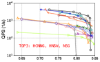
(a) Recall@10 (UQ-V)

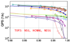
(b) Recall@10 (Msong)

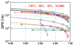
(c) Recall@10 (SIFT1M)

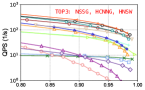
(d) Recall@10 (GIST1M)

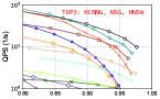
(e) Recall@10 (GloVe)

Figure 7. The Queries Per Second (QPS) vs Recall@10 of graph-based ANNS algorithms in high-precision region (top right is better).

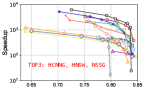
(a) Recall@10 (UQ-V)

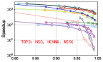
(b) Recall@10 (Msong)

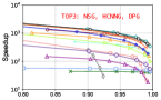
(c) Recall@10 (SIFT1M)

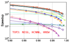
(d) Recall@10 (GIST1M)

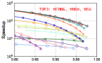
(e) Recall@10 (GloVe)

Figure 8. The Speedup vs Recall@10 of graph-based ANNS algorithms in high-precision region (top right is better).

Memory overhead (MO). As Table 5 show, RNG-based algorithms generally have the smallest memory overhead (e.g., NSG and NSSG). Some algorithms with additional index structures have high memory overhead (e.g., SPTAG and IEH). Larger AD and CS values also will increase the algorithms’ memory overhead (e.g., NSW and SPTAG-BKT). Overall, the smaller the algorithm’s index size, the smaller the memory overhead during search.

5.4. Components’ Evaluation

In this subsection, we evaluate representative components of graph-based algorithms on two real-world datasets with different difficulty. According to the aforementioned experiments, algorithms based on the Refinement construction strategy generally have better comprehensive performance. Therefore, we design a unified evaluation framework based on this strategy and the pipline in Figure 4. Each component in the evaluation framework is set for a certain implementation to form a benchmark algorithm (see Appendix K for detailed settings). We use the C# + algorithm name to indicate the corresponding component’s specific implementation. For example, C1_NSG indicates that we use the initialization (C1) of NSG, i.e., the initial graph is constructed through NN-Descent.

Note that many algorithms have the same implementation for the same component (e.g., C3_NSG, C3_HNSW, and C3_FANNG). We randomly select an algorithm to represent this implementation (e.g., C3_HNSW). The impact of different components on search performance and construction time are depicted in Figure 10 and Appendix M, respectively.

Table 5. The candidate set size (CS), query path length (PL), and peak memory overhead (MO) during the search (the bold values are the best).

Alg.	UQ-V			Msong			Audio			SIFT1M			GIST1M			Crawl			GloVe			Enron
	CS	PL	MO	CS	PL	MO	CS	PL	MO	CS	PL	MO	CS	PL	MO	CS	PL	MO	CS	PL	MO	CS	PL	MO
KGraph	15,000+	1,375	1,211	50,442	1,943	2,036	701	105	55	139	52	900	2,838	411	4,115	50,000+	3,741	3,031	24,318	1,333	991	9,870	607	525
NGT-panng	65	79	1,423	10	144	1,927	10	33	63	20	438	933	10	1,172	4,111	10	5,132	3,111	10	2,281	928	10	83	535
NGT-onng	1,002	431	1,411	20	227	2,007	15	45	63	33	392	859	33	1,110	4,088	157	244	3,147	74	388	1,331	25	131	533
SPTAG-KDT	37,097	2,259	2,631	50,000+	11,441	2,091	61	107	91	7,690	1,227	1,048	50,000+	15,162	5,643	50,000+	12,293	8,872	50,000+	10,916	11,131	10,291	592	569
SPTAG-BKT	15,000+	10,719	5,114	97,089	11,119	1933	10	61	91	50,000+	8,882	4,587	50,000+	7,685	4,299	50,000+	10,851	6,643	50,000+	7,941	4,625	93,294	5,126	629
NSW	85	38	1,857	20	35	3,122	18	17	101	58	54	1,574	69	161	5,180	36	435	5,217	65	634	2,782	21	29	690
IEH	29	196	5,166	301	1,007	6,326	53	269	253	238	816	4,170	9,458	24,339	10,508	15,000+	5,928	10,913	15,000+	3,620	4,681	274	893	1,302
FANNG	1,072	86	1,395	594	245	1,687	1,462	195	58	1,377	92	825	3,007	269	3,917	8,214	2,152	2,639	9,000	1,062	850	2,084	152	548
HNSW	927	296	1,424	43	35	2,370	51	37	67	66	47	1,206	181	130	4,372	61	108	3,950	505	334	1,294	59	32	595
EFANNA	1,446	217	1,297	312	85	2,030	800	283	67	204	76	967	1,652	292	4,473	1311	180	3,848	22,349	1241	1,188	2,180	254	531
DPG	15,000+	1,007	1,352	16	20	1,965	10	10	62	37	30	851	55	124	4,091	67	761	3,089	84	792	956	89	60	538
NSG	354	156	1,127	106	90	1,714	63	47	51	101	85	653	867	826	3,781	345	723	2,499	814	1,875	594	118	138	513
HCNNG	15,000+	1,398	1,472	62	21	2,200	35	12	69	97	37	1,056	371	179	4,159	173	61	3,753	217	95	1,590	62	20	564
Vamana	1,049	346	1,164	40,596	7,155	1,763	68	30	57	493	263	748	8,360	3,127	3,916	53,206	7,465	2,786	22,446	2,157	1026	526	103	547
NSSG	310	122	1,129	39	40	1,807	65	42	51	255	157	640	280	270	3,829	13,810	12,892	2,524	3,846	3,047	605	458	236	514

C1: Initialization. Figure 10(a) reports the impact of different graph index initialization methods on search performance. The search performance of C1_NSG is much better than C1_EFANNA and C1_KGraph; and although C1_NSG needs more construction time, it is worthwhile for such a large performance improvement. Moreover, a larger gap exists between C1_NSG and the other two on GIST1M (harder), which shows that it has better scalability.

C2: Candidate neighbor acquisition. As shown in Figure 10(b), different candidate neighbor acquisition methods vary slightly. C2_NSW has the best search performance, especially on GIST1M, with the price being more construction time. C2_NSSG obtains better search performance than C2_DPG under a similar construction time. It is worth noting that although DPG’s search performance on SIFT1M is better than HNSW’s in Figure 7, the search performance of C2_HNSW (i.e., C2_NSW) exceeds that of C2_DPG.

C3: Neighbor selection. Figure 10(c) depicts the impact of different neighbor selection schemes on search performance. Obviously, it shows better search performance for algorithms that consider the distribution of neighbors (e.g., C3_HNSW, C3_NSSG, C3_DPG, C3_Vamana) than those that do not consider this (e.g., C3_KGraph). Note that C3_Vamana’s performance is no better than C3_HNSW’s, as claimed in the paper (Subramanya et al., 2019). NSSG(Fu et al., 2021) appears to have better search performance than NSG in their experiment, so the researchers believe that C3_NSSG is better than C3_NSG (i.e., C3_HNSW). However, the researchers do not control the consistency of other components during the evaluation, which is unfair.

Table 6. Index processing time (IPT) and memory consumption (MC) of ML1-based optimization.

Method		SIFT100K	GIST100K
IPT(s)	NSG	55	142
	NSG+ML1	55+67,260	142+45,600
MC(GB)	NSG	0.37	0.68
	NSG+ML1	23.8	58.7

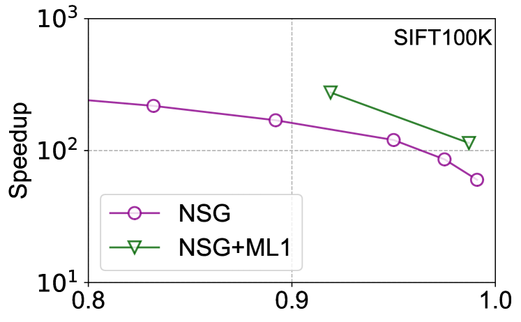
Figure 9. Speedup vs Recall@1 of NSG under ML1-based optimizations.

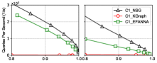
(a) Recall@10 on SIFT1M (left) and GIST1M (right)

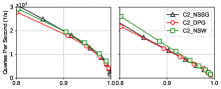
(b) Recall@10 on SIFT1M (left) and GIST1M (right)

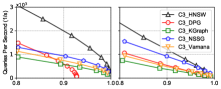
(c) Recall@10 on SIFT1M (left) and GIST1M (right)

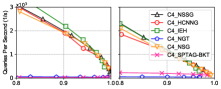
(d) Recall@10 on SIFT1M (left) and GIST1M (right)

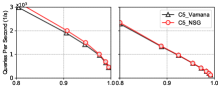
(e) Recall@10 on SIFT1M (left) and GIST1M (right)

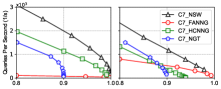
(f) Recall@10 on SIFT1M (left) and GIST1M (right)

Figure 10. Components’ search performance under a unified framework on SIFT1M (a simple dataset) and GIST1M (a hard dataset).

C4: Seed preprocessing and C6: Seed acquisition. The C4 and C6 components are interrelated in all compared algorithms; that is, after specifying C4, C6 is also determined. Briefly, we use C4_NSSG to indicate C6_NSSG. As Figure 10(d) shows, the extra index structure to get the entry significantly impacts search performance. C4_NGT and C4_SPTAG-BKT have the worst search performance; they both obtain entry by performing distance calculations on an additional tree (we know that the tree index has a serious curse of dimensionality). Although C4_HCNNG also obtains entry through a tree, it only needs value comparison and no distance calculation on the KD-Tree, so it shows better search performance than C4_NGT and C4_SPTAG-BKT. C4_IEH adds the hash table to obtain entry, yielding the best search performance. This may be because the hash can obtain entry close to the query more quickly than the tree. Meanwhile, C4_NSSG and C4_NSG still achieve high search performance without additional index. Note that there is no significant difference in index construction time for these methods.

C5: Connectivity. Figure 10(e) shows the algorithm with guaranteed connectivity has better search performance (e.g., C5_NSG) than that without connectivity assurance (e.g., C5_Vamana).

C7: Routing. Figure 10(f) shows different routing strategies’ impact on search performance. C7_NSW’s search performance is the best, and it is used by most algorithms (e.g., HNSW and NSG). C7_NGT has a precision “ceiling” because of the $\epsilon$ parameter’s limitation, which can be alleviated by increasing $\epsilon$, but search efficiency will decrease. C7_FANNG can achieve high accuracy through backtracking, but backtracking also limits search efficiency. C7_HCNNG avoids some redundant calculations based on the query position, however, this negatively affects search accuracy.

Table 7. Recommendation of the algorithms in different scenarios.

Scenario	Algorithm
S1: A large amount of data updated frequently	NSG, NSSG
S2: Rapid construction of KNNG	KGraph, EFANNA, DPG
S3: Data is stored in external memory	DPG, HCNNG
S4: Search on hard datasets	HNSW, NSG, HCNNG
S5: Search on simple datasets	DPG, NSG, HCNNG, NSSG
S6: GPU acceleration	NGT
S7: Limited memory resources	NSG, NSSG

5.5. Machine Learning-Based Optimizations

Recently, machine learning (ML)-based methods are proposed to improve the speedup vs recall trade-off of the algorithms (Baranchuk et al., 2019; Li et al., 2020; Prokhorenkova and Shekhovtsov, 2020). In general, they can be viewed as some optimizations on graph-based algorithms discussed above (such as NSG and NSW). We evaluate three ML-based optimizations on NSG and HNSW, i.e., ML1 (Baranchuk et al., 2019), ML2 (Li et al., 2020), and ML3 (Prokhorenkova and Shekhovtsov, 2020). Because of space limitations, we only show the test results on ML1 in Table 6 and Figure 9, others share similar feature (see Appendix R for more details).

Analysis. ML-based optimizations generally obtain better speedup vs recall tradeoff at the expense of more time and memory. For example, the original NSG takes 55s and maximum memory consumption of 0.37 GB for index construction on SIFT100K; however, NSG optimized by ML1 takes 67,315s to process the index (even if we use the GPU for speedup), and the memory consumption is up to 23.8 GB. In summary, current ML-based optimizations have high hardware requirements and time cost, so their wide application is limited. Considering that most of the original graph-based algorithms can return query results in ¡ 5ms, some high-tech companies (such as Alibaba, Facebook, and ZILLIZ) only deploy NSG without ML-based optimizations in real business scenarios (Fu et al., 2019; Johnson et al., 2017; Milvus, 2019).

6. Discussion

According to the behaviors of algorithms and components on real-world and synthetic datasets, we discuss our findings as follows.

Recommendations. In Table 7, our evaluation selects algorithms based on best performance under different scenarios. NSG and NSSG have the smallest construction time and index size, so they are suitable for S1. KGraph, EFANNA, and DPG achieve the highest graph quality with lower construction time, so they are recommended for S2. For S3 (such as SSD (Subramanya et al., 2019)), DPG and HCNNG are the best choices because their smaller average path length can reduce I/O times. On hard datasets (S4, large LID), HNSW, NSG, and HCNNG show competitive search performance, while on simple datasets (S5), DPG, NSG, HCNNG, and NSSG offer better search performance. For S6, we need a smaller candidate set size because of the cache’s limitation (Zhao et al., 2020); for now, NGT appears more advantageous. NSG and NSSG offer the smallest out-degree and memory overhead, so they are the best option for S7.

Guidelines. Intuitively, a practical graph-based ANNS algorithm should have: (H1) high construction efficiency; (H2) high routing efficiency; (H3) high search accuracy; and (L4) low memory overhead. For H1, we should not spend too much time improving graph quality, because the best graph quality is not necessary to achieve the best search performance. For H2, we should control the appropriate out-degree, diversify neighbors’ distribution (such as C3_HNSW), and reduce the cost of obtaining entries (like C4_IEH), to navigate quickly to the query’s nearest neighbors with a small number of distance calculations. In addition, we should avoid redundant distance calculations by optimizing the routing strategy (such as C7_HCNNG) in the routing process. In terms of H3, to improve the search’s immunity from falling into the local optimum (Baranchuk et al., 2019), we should reasonably design the distribution of neighbors during index construction, ensure connectivity (such as C5_NSG), and optimize the routing strategy (Vargas Muñoz et al., 2019). For L4, we can start by reducing the out-degree and candidate set size, and this can be achieved by improving the neighbor selection strategy (such as C3_NSG) and routing strategy (like C7_HCNNG).

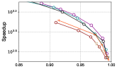
(a) Recall@10 (Msong)

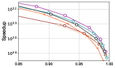
(b) Recall@10 (SIFT1M)

Figure 11. Speedup vs Recall@10 of the optimized algorithm (OA).

Improvement. Based on our observations and Guidelines, we design an optimized algorithm that addresses H1, H2, H3, and L4 simultaneously. In the index construction phase, it initializes a graph with appropriate quality by NN-Descent (C1), quickly obtains candidate neighbors with C2_NSSG (C2), uses C3_NSG to trim redundant neighbors (C3), randomly selects a certain number of entries (C4), and ensures connectivity through depth-first traversal (C5); in the search phase, it starts from the random entries (C6), and performs two-stage routing through C7_HCNNG and C7_NSW in turn. As shown in Figure 11, the optimized algorithm surpasses the state-of-the-art algorithms in terms of efficiency vs accuracy trade-off, while ensuring high construction efficiency and low memory overhead (see Appendix P for more details).

Tendencies. Over the last decade, graph-based ANNS algorithms have ranged from simple approximation of four classic base graphs (e.g., KGraph and NSW) to ANNS’s optimization (e.g., HNSW and NSG). Along the way, their performance—especially their search performance—has improved qualitatively. It is worth noting that almost all state-of-the-art algorithms are based on RNG (e.g., HNSW and NSG), and thus many approaches add an approximation of RNG on the basis of KNNG- or DG-based algorithms (see Figure 3). The RNG-based category is still a promising research direction for graph-based ANNS. The MST-based algorithm recently was applied to graph-based ANNS, and it also achieves excellent results in our evaluation, especially on hard datasets. On the basis of the core algorithm discussed in this paper, researchers are refining and improving graph-based ANNS algorithms’ performance via hardware (Subramanya et al., 2019; Zhao et al., 2020; Jie Ren et al., 2020). Other literatures add quantitative or distributed schemes to cope with data increases (Douze et al., 2018; Deng et al., 2019). To meet hybrid query requirements, the latest research adds structured attribute constraints to the search process of graph-based algorithms (Wei et al., 2020; Xu et al., 2020).

Challenges. At present, almost all graph-based algorithms are oriented to raw data, which is the main reason why these algorithms have high memory usage. Determining how to organically combine data encoding or other methods with graph-based ANNS algorithms is a problem worth exploring. Compared with tree, hashing, and quantization, the graph-based algorithms have the highest index construction time (Li et al., 2019), which adds difficulty with updating the graph index in real time. Also, figuring how to combine GPU acceleration or other methods with the graph-based ANNS algorithm to realize the real-time update of the graph index is worthy of an in-depth study. For data with different characteristics, the graph-based algorithms have different adaptability, and thus exhibit different performance levels. Finally, a major outstanding challenge is discerning how to adaptively select the optimal graph-based algorithm according to the dataset’s characteristics by learning.

7. Conclusions

In this paper, we consider 13 representative graph-based ANNS algorithms from a new taxonomy. We then divide all the algorithms into seven components for in-depth analysis. Next, we comprehensively evaluate and discuss all the algorithms’ performance on eight real-world datasets and 12 synthetic datasets. We also fairly evaluate each algorithm’s important components through a unified framework. In some ways, this work validates many previous empirical conclusions while leading to novel discoveries that will aid future researchers and practitioners. We also provide some rule-of-thumb recommendations about promising research directions and insightful principles to optimize algorithms.

Finally, we want to note that because of various constraints, our study only investigates core algorithms based on the main memory. Going forward, we will consider hardware (e.g., SSD and GPU) and machine learning optimizations, deploy distributed implementations, and add structured attribute constraints to ANNS.

Appendix

Appendix A. Proof for the equivalence of the neighbor selection strategies of HNSW and NSG

Notations. Given any point $p$ on dataset $S$, the candidate neighbor set of $p$ obtained before neighbor selection is marked as $\mathcal{C}$ (see Definition 4.4 for the definition of candidate neighbor acquisition), and the neighbor selection (Definition 4.5) gets the final neighbor set $N(p)$ from $\mathcal{C}$ for $p$. $\mathcal{B}(p,r)$ denotes an open sphere such that $\mathcal{B}(p,r)=\left\{x|\delta(p,x)<r,x\in S\right\}$, where $r$ is a constant. $lune_{pm}$ denotes a region such that $lune_{pm}=\mathcal{B}(p,\delta(p,m))\cap\mathcal{B}(m,\delta(m,p))$.

The neighbor selection strategy of HNSW. In the original paper of HNSW (Malkov and Yashunin, 2018), the neighbor selection strategy is called heuristic neighbor selection. When selecting neighbors for the inserted point $p$, HNSW regards $p$ as a query to perform ANNS on the constructed partial graph index to obtain a certain amount of its nearest neighbors as candidate neighbors $\mathcal{C}$. Next, the heuristic neighbor selection iteratively gets the unvisited point $m$ that has the smallest $\delta(m,p)$ from $\mathcal{C}$, if $\forall n\in N(p)$, $\delta(m,n)>\delta(m,p)$ (Condition 1), then $N(p)\cup\left\{m\right\}$, otherwise, $m$ will be discarded. For more details, please see the Algorithm 4 in the original publication of HNSW (Malkov and Yashunin, 2018).

The neighbor selection strategy of NSG. In the original paper of NSG (Fu et al., 2019), the neighbor selection strategy is called edge selection strategy of Monotonic Relative Neighborhood Graph (MRNG). When selecting neighbors for $p$, MRNG gets the unvisited point $m$ with the smallest $\delta(m,p)$ from $\mathcal{C}$. Iff $lune_{pm}\cap\mathcal{C}=\emptyset$ or $\forall u\in(lune_{pm}\cap\mathcal{C})$, $u\not\in N(p)$ (Condition 2), then $N(p)\cup\left\{m\right\}$. For more details, please refer to the Algorithm 2 in the original publication of NSG (Fu et al., 2019).

Below we prove the equivalence of the neighbor selection of the two.

Proof.

First, we prove that the neighbor selection of NSG can be derived from the neighbor selection of HNSW. For any point $m\in\mathcal{C}$ that can be added to $N(p)$, we only need to prove that if Condition 1 is satisfied, then Condition 2 must be satisfied. For Condition 1: $\forall n\in N(p)$, $\delta(m,n)>\delta(m,p)$, we can infer that $\forall n\in N(p)$ must satisfy $n\not\in\mathcal{B}(m,\delta(m,p))$, otherwise, there will $\exists n\in N(p)$ makes $\delta(m,n)<\delta(m,p)$. Thus, we have

$$lune_{pm}\cap N(p) =\mathcal{B}(p,\delta(p,m))\cap\mathcal{B}(m,\delta(m,p))\cap N(p)$$

$$=\mathcal{B}(p,\delta(p,m))\cap\emptyset$$

$$=\emptyset$$

Since $N(p)$ are all selected from $\mathcal{C}$, that is, $N(p)\subset\mathcal{C}$, below, we will discuss whether $lune_{pm}\cap(\mathcal{C}\setminus N(p))$ is $\emptyset$.

(1) Suppose $lune_{pm}\cap(\mathcal{C}\setminus N(p))=\emptyset$. Then, we have

$$lune_{pm}\cap\mathcal{C} =lune_{pm}\cap((\mathcal{C}\setminus N(p))\cup N(p))$$

$$=(lune_{pm}\cap(\mathcal{C}\setminus N(p)))\cup(lune_{pm}\cap N(p))$$

$$=\emptyset\cup\emptyset$$

$$=\emptyset$$

Condition 1 is satisfied.

(2) Suppose $lune_{pm}\cap(\mathcal{C}\setminus N(p))\not=\emptyset$. Obviously, $lune_{pm}\cap\mathcal{C}\not=\emptyset$, because $lune_{pm}\cap N(p)=\emptyset$, so $\forall u\in(lune_{pm}\cap\mathcal{C})$ must have

$$u\in lune_{pm}\cap(\mathcal{C}\setminus N(p))=(lune_{pm}\cap\mathcal{C})\setminus N(p)$$

That is, $u\not\in N(p)$. Condition 1 is satisfied.

Therefore, if Condition 1 is established, then Condition 2 must be established.

Next, we prove that the neighbor selection of HNSW can be derived from the neighbor selection of NSG. For any point $m\in\mathcal{C}$ that can be added to $N(p)$, we only need to prove that if Condition 2 is satisfied, then Condition 1 must be satisfied. For Condition 2: $lune_{pm}\cap\mathcal{C}=\emptyset$ or $\forall u\in(lune_{pm}\cap\mathcal{C})$, $u\not\in N(p)$, we discuss the two cases of $lune_{pm}\cap\mathcal{C}=\emptyset$ and $\forall u\in(lune_{pm}\cap\mathcal{C})$, $u\not\in N(p)$ separately.

(1) When $lune_{pm}\cap\mathcal{C}=\emptyset$ is established, because $N(p)\subset\mathcal{C}$, therefore, $lune_{pm}\cap N(p)=\emptyset$. Since the unvisited point $m$ with the smallest $\delta(m,p)$ is taken from $\mathcal{C}$ every time, that is, $\forall n\in N(p)$, $\delta(n,p)<\delta(m,p)$, thus, $\forall n\in N(p)$, $n\in\mathcal{B}(p,\delta(p,m))$, and we have

$$n\not\in \mathcal{B}(m,\delta(m,p))\setminus\mathcal{B}(p,\delta(p,m))$$

$$=\mathcal{B}(m,\delta(m,p))\setminus(\mathcal{B}(m,\delta(m,p))\cap\mathcal{B}(p,\delta(p,m)))$$

$$=\mathcal{B}(m,\delta(m,p))\setminus lune_{pm}$$

Since $lune_{pm}\cap N(p)=\emptyset$, then $\forall n\in N(p)$, $n\not\in lune_{pm}$, so

$$n\not\in(\mathcal{B}(m,\delta(m,p))\setminus lune_{pm})\cup lune_{pm}=\mathcal{B}(m,\delta(m,p))$$

Thus, $\forall n\in N(p)$, $\delta(m,n)>\delta(m,p)$, Condition 1 is satisfied.

(2) When $\forall u\in(lune_{pm}\cap\mathcal{C})$, $u\not\in N(p)$, it is easy to know that $\forall n\in N(p)$, $n\not\in(lune_{pm}\cap\mathcal{C})$. Thus, $n\not\in lune_{pm}$, otherwise, if $n\in lune_{pm}$, $n\in\mathcal{C}$ is known, then $\exists n\in N(p)$ makes $n\in(lune_{pm}\cap\mathcal{C})$, which contradicts the known. Since $n\not\in\mathcal{B}(m,\delta(m,p))\setminus lune_{pm}$, we have

$$n\not\in lune_{pm}\cup(\mathcal{B}(m,\delta(m,p))\setminus lune_{pm})=\mathcal{B}(m,\delta(m,p))$$

Thus, $\forall n\in N(p)$, $\delta(m,n)>\delta(m,p)$, Condition 1 is satisfied.

Therefore, if Condition 2 is established, then Condition 1 must be established.

In summary, the neighbor selection strategies of HNSW and NSG are equivalent. ∎

Appendix B. Proof for the path adjustment of NGT is an approximation to the neighbor selection of RNG

Path adjustment. We can formally describe the path adjustment as follows. Given graph $G(V,E)$, $N(p)$ is the current neighbor set of $p\in V$. As shown in Figure 12, if there is an alternative path $p\rightarrow x\rightarrow n$ with length $l=2$ (the number of edges) between $p$ and $n$, where $n\in N(p)$, then do the following: If $\max\left\{\delta(p,x),\delta(x,n)\right\}<\delta(p,n)$, then delete $n$ from $N(p)$, otherwise keep $n$. If there is no alternative path between $p$ and $n$ or the length $l\not=2$ of the alternative path, then $n$ is also reserved. For more details about path adjustment, please refer to the original paper (Iwasaki and Miyazaki, 2018).

The neighbor selection of RNG. Given any point $p$ on dataset $S$, the candidate neighbor set of $p$ is $\mathcal{C}$, gets the unvisited point $m$ that has the smallest $\delta(m,p)$ from $\mathcal{C}$, if $\forall n\in N(p)$, $\delta(m,n)>\delta(m,p)$, then $N(p)\cup\left\{m\right\}$, otherwise, $m$ will be discarded (Harwood and Drummond, 2016).

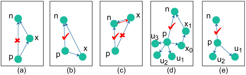
Figure 12. The path adjustment of NGT (Iwasaki and Miyazaki, 2018).

Next, we prove that the above path adjustment operation is an approximate implementation of neighbor selection of RNG. Given vertex $p$ on $G(V,E)$, the neighbors $N(p)$ of $p$ is sorted in ascending order according to the distance between each neighbor and $p$, and the neighbors are visited in this order when conducting path adjustment. Therefore, the selection way of visited vertex for path adjustment is consistent with neighbor selection of RNG. We only need to prove that the judgment criteria of the visited vertex cut or retained is an approximation to that of RNG.

Proof.

We conduct the discussion based on the alternative path length $l$ between $p$ and $n$.

(1) As shown in Figure 12 (a), (b), and (c), when the length $l=2$ of alternative path $p\rightarrow x\rightarrow n$ between $p$ and $n$, there are two situations:

• If $\max\left\{\delta(p,x),\delta(x,n)\right\}<\delta(p,n)$ (Figure 12 (a)), then $n$ will be deleted. It is easy to know that $\delta(p,n)>\delta(x,n)$, which is consistent with the neighbor selection of RNG.

• If $\max\left\{\delta(p,x),\delta(x,n)\right\}>\delta(p,n)$ (Figure 12 (b) and (c)), then $n$ will be reserved. At this time, when $\delta(p,n)<\delta(x,n)$ (Figure 12(b)), the neighbor selection of RNG is met; When $\delta(p,n)>\delta(x,n)$ (Figure 12(c)), then $\delta(p,n)<\delta(p,x)$. Since $\delta(x,n)$ is small, $n\in N(x)$ has a high probability of occurrence. We know that $x\in N(p)$, when judging whether there is an alternative path between $p$ and $x$, since the alternative path $(p\rightarrow n\rightarrow x)$ exists, and satisfies $\delta(p,n)<\delta(p,x)$ and $\delta(n,x)<\delta(p,x)$, that is, $\max\left\{\delta(p,n),\delta(n,x)\right\}<\delta(p,x)$, thus, $x$ needs to be deleted. At this time, keeping $n$ and deleting $x$ is consistent with the result of the neighbor selection of RNG.

(2) As shown in Figure 12(d), when there is an alternative path with length $l>2$ between $p$ and $n$, it means that the distance between $n$ and $p$ is likely to be farther, so that most of the neighbors of $n$ and $p$ are far away. Therefore, $\delta(n,p)<\delta(n,u)$ is easy to hold for most $u$, and $u$ is one of the neighbors of $p$ except $n$. In this case, the results of keeping $n$ is consistent with the neighbor selection of RNG.

(3) As shown in Figure 12(e), if there is no alternative path between $p$ and $n$, it means that there is a high probability that $p$ is closer to $n$, so $\delta(p,n)<\delta(u,n)$ for most $u$, $u$ is one of the neighbors of $p$ except $n$. In this case, the results of keeping $n$ is consistent with the neighbor selection of RNG.

In summary, the path adjustment of NGT is an approximation to the neighbor selection of RNG. ∎

Appendix C. Proof for the neighbor selection of DPG is an approximation to that of RNG

Overview. According to Appendix A and Appendix B, the neighbor selection of RNG can be approximately described by the neighbor selection of HNSW. Due to the equivalence of the neighbor selection strategies of HNSW and NSG, we can represent the neighbor selection of RNG by the neighbor selection of NSG (Appendix A). Therefore, we only need to prove that the neighbor selection of DPG is an approximation to that of NSG.

The neighbor selection of DPG. The construction of DPG is a diversification of the KGraph (Dong, 2011), followed by adding reverse neighbors. Given any a vertex $p$ on $G(V,E)$, $\mathcal{C}$ is the candidate neighbor set of $p$, $\theta(x,y)$ denotes $\measuredangle xpy$, where $x,y\in\mathcal{C}$. The neighbor selection of DPG aims to choose a subset $N(p)$ of $\kappa$ vertices from $\mathcal{C}$ so that $N(p)=\arg\max_{N(p)\subseteq\mathcal{C}}\sum_{x,y\in\mathcal{C}}\theta(x,y)$. For full details, please see the original publication of DPG (Li et al., 2019).

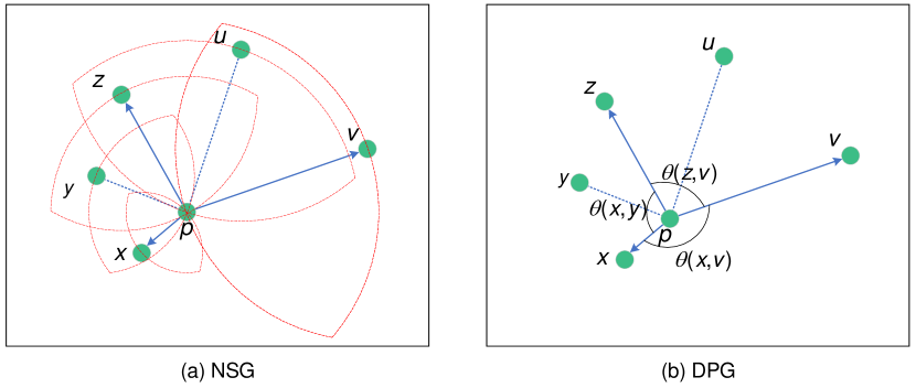
Figure 13. The neighbor selection of NSG and DPG.

Lemma 7.1.

Given the $G(V,E)$ constructed by the neighbor selection of NSG, any a vertex $p\in V$ and the neighbor set $N(p)$ of $p$ on $G(V,E)$. $\forall x,y\in N(p)$, $\measuredangle xpy\geq 60^{\circ}$.

We prove Lemma 7.1 as follows.

Proof.

As shown in Figure 13(a), for the $N(p)$ obtained from $\mathcal{C}$ by the neighbor selection of NSG (Appendix A), if $\exists x,y\in N(p)$, and $\measuredangle xpy<60^{\circ}$, then we can know that $\measuredangle pyx+\measuredangle pxy>120^{\circ}$ in $\triangle xpy$, thus, there must be $\measuredangle pyx>60^{\circ}$ or $\measuredangle pxy>60^{\circ}$.

Suppose $\delta(p,y)>\delta(p,x)$, then $\measuredangle pxy>60^{\circ}$ (i.e., the situation shown in Figure 13(a)), we know that $\measuredangle pxy>\measuredangle xpy$, so $\delta(p,y)>\delta(x,y)$, we have $x\in\mathcal{B}(y,\delta(p,y))$. Since $\delta(p,y)>\delta(p,x)$, so $x\in\mathcal{B}(p,\delta(p,y))$, it is easy to know that $x\in\mathcal{B}(y,\delta(p,y))\cap\mathcal{B}(p,\delta(p,y))=lune_{py}$. However, $x\in N(p)$, according to the neighbor selection strategy of NSG (Appendix A), $y$ cannot be added to $N(p)$, which contradicts the known ($y\in N(p)$).

When $\delta(p,y)<\delta(p,x)$, we can just swap the positions of $x$ and $y$ above, and then get the same conclusion.

Therefore, Lemma 7.1 is proved. ∎

Now we prove that the neighbor selection of DPG is an approximation to that of NSG.

Proof.

As shown in Figure 13(a), when selecting neighbors for $p$, it needs to determine whether a point in $\mathcal{C}=\left\{x,y,z,u,v\right\}$ can be added to $N(p)$ according to the neighbor selection of NSG, and finally $N(p)=\left\{x,z,v\right\}$. It can be seen that $\forall x,y\in N(p)$, $\measuredangle xpy\geq 60^{\circ}$ from Lemma 7.1.

Figure 13(b) is based on the neighbor selection strategy of DPG, which selects $\kappa=3$ neighbors to $N(p)$ from $\mathcal{C}=\left\{x,y,z,u,v\right\}$ to maximize the sum of angles between neighbors. From this, it can be inferred that $\exists\hat{\theta}\in[0^{\circ},180^{\circ}]$, for $\forall v_{1},v_{2}\in N(p)$, $\theta(v_{1},v_{2})\geq\hat{\theta}$. When $\hat{\theta}=60^{\circ}$, that is, $\hat{\theta}\geq 60^{\circ}$, which ensures the result of neighbor selection of NSG.

Therefore, we can say that the neighbor selection of DPG is an approximation to that of NSG, and thus an approximation to that of RNG. ∎

Appendix D. Complexity analysis

Since the construction or search complexity of some graph-based ANNS algorithms were not informed by the authors, we deduce the approximate complexity based on the description of the algorithm and our experimental evaluation. In order to make the evaluation results more general, we carefully select the characteristics of the dataset, which are shown in Table 8. The standard deviation is the standard deviation of the distribution in each cluster.

For index construction complexity, we record the index construction time under different scales and calculate the functional relationship between the two. As for search complexity, we count the number of distance evaluations under a given recall rate, considering that distance evaluation occupies the main search time (Zhao et al., 2020). Note that the relevant parameters used in the evaluation process are the optimal parameters obtained by grid search (see our online publication for more details). All experimental evaluation codes remove parallel commands and use single-threaded program execution on a Linux server with Intel(R) Core(TM) i9-10900X CPU at 3.70GHz, and 125G memory.

Table 8. Characteristics of the dataset for complexity evaluation

# Base	# Query	Dimension	# Cluster	Standard deviation
$10^{5}\sim 10^{6}$	$10^{3}$	32	10	5

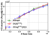
(a) Search complexity of KGraph

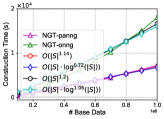
(b) Construction complexity of NGT

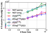
(c) Search complexity of NGT

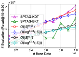
(d) Search complexity of SPTAG

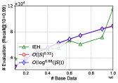
(e) Search complexity of IEH

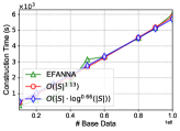
(f) Construction complexity of EFANNA

(g) Search complexity of EFANNA

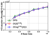
(h) Search complexity of DPG

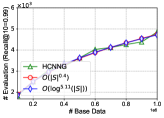
(i) Search complexity of HCNNG

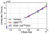
(j) Construction complexity of Vamana

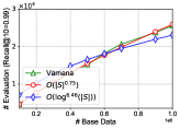
(k) Search complexity of Vamana

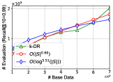
(l) Search complexity of k-DR

Figure 14. Complexity evaluation. # Base is the size of base dataset, and # Evaluation is the number of distance evaluations.

KGraph. We set $Recall@10=0.99$ and evaluate how the number of distance evaluations with the data size. As shown in Figure 14(a), the complexity of search on KGraph is about $O(|S|^{0.54})$. When the size of the dataset is small ($<0.6\times 10^{6}$), the search complexity of KGraph is lower than that of $O(\log^{6.07}(|S|))$. However, as the size of the dataset increases, the search complexity of KGraph is slightly higher than $O(\log^{6.07}(|S|))$.

NGT. There are two main versions of NGT, NGT-panng and NGT-onng respectively. The main difference between the two is that NGT-onng has one extra step that out-degree and in-degree adjustment than NGT-panng (Iwasaki, 2015). According to the evaluation results in Figure 14(b) and (c), NGT-onng requires a larger construction time than NGT-panng due to additional out-degree and in-degree adjustment. However, NGT-onng has not received better search performance than NGT-panng, the search complexity of the two is very close, and NGT-panng has higher efficiency in the evaluation dataset, which shows that the effectiveness of out-degree and in-degree adjustment needs to be further verified.

SPTAG. We implement two versions of SPTAG, SPTAG-KDT and SPTAG-BKT respectively. SPTAG-KDT is the original version, which corresponds to the description of the paper (Wang and Li, 2012; Wang et al., 2012, 2013b). SPTAG-BKT is an optimized version based on SPTAG-KDT, the specific description can refer to the online project  (Chen et al., 2018). As shown in Figure 14(d), SPTAG-KDT ($O((|S|^{0.68})$) and SPTAG-KMT ($O((|S|^{0.7})$) have approximately the same search time complexity. However, under the same dataset size, SPTAG-BKT requires fewer distance evaluation times, that is, SPTAG-BKT mainly optimizes the constant part of search complexity.

NSW. In (Malkov et al., 2014), the authors give that the search complexity of NSW is $O(\log^{2}(|S|))$ by experiment. For index construction, NSW is based on the idea that graph structure is assembled by inserting elements one by one and connects them with a certain amount of nearest neighbors at each step. These nearest neighbors connected to each vertex is obtained by greedy search on the already constructed graph. As the time complexity of inserting each vertex is $O(\log^{2}(|S|))$, the complexity of constructing NSW on the dataset $S$ is $O(|S|\cdot\log^{2}(|S|))$.

IEH. In (Jin et al., 2014), the authors report that the construction complexity of KNN table is $O(|S|^{2}\cdot(d+\log{(|S|)})$, where $d$ is the dimensionality and $d\ll|S|$. As we all know, the complexity of building a hash bucket is much less than $O(|S|^{2}\cdot(\log{(|S|)})$. Therefore, the construction complexity of IEH is $O(|S|^{2}\cdot\log(|S|)+|S|^{2})$. In Figure 14(e), the search complexity of IEH is about $O(|S|^{0.52})$. However, under the same dataset size, IEH requires more distance evaluations than most other algorithms.

EFANNA. The construction process of EFANNA is very similar to KGraph except for the initialization. KGraph initializes the neighbors of each vertex randomly, while EFANNA uses KD-trees to initialize the neighbors more accurately. From Figure 14(f), we can see that the construction complexity of EFANNA is about $O(|S|^{1.13})$, which is very close to KGraph. It shows that EFANNA’s optimization to KGraph only changes the constant factor of the construction complexity. Since both are constructing a KNNG with high quality, the search complexity of KGraph ($O(|S|^{0.54})$) and EFANNA ($O(|S|^{0.55})$) are also very similar in Figure 14(a) and (g).

DPG. The construction process of DPG includes two steps: (1) a KNNG construction and (2) the diversification of the KNNG. For the first step, the time complexity of constructing KNNG through NN-Descent on the dataset $S$ is $O(|S|^{1.14})$. The second step is the process of pruning edges on the KNNG constructed in the previous step to maximize the angle between neighbors, followed by adding reverse edges (Appendix C). For the vertex $p$ on KNNG, $p$’s neighbor set is $\mathcal{C}=\left\{v_{0},v_{1},\cdots,v_{\kappa-1}\right\}$, in which elements are sorted in ascending order of distance from $p$, and $|\mathcal{C}|=\kappa$, the result neighbor set is $N(p)$ and initialized to $\emptyset$ for DPG. At the beginning of selecting neighbors for $p$ (the first iteration), we add $v_{0}$ to $N(p)$ and $\mathcal{C}\setminus\left\{v_{0}\right\}$ ($|\mathcal{C}|=\kappa-1$, $|N(p)|=1$); In the second iteration, we select $v_{i}\in\mathcal{C}$ to maximize $\measuredangle v_{i}pv_{0}$, then let $N(p)\cup\left\{v_{i}\right\}$ and $\mathcal{C}\setminus\left\{v_{i}\right\}$ ($|\mathcal{C}|=\kappa-2$, $|N(p)|=2$), it requires $\kappa-1$ calculations for selecting such a $v_{i}$; In the third iteration, we select $v_{j}\in\mathcal{C}$ so that $\measuredangle v_{j}pv_{0}+\measuredangle v_{j}pv_{i}$ is maximized, then let $N(p)\cup\left\{v_{j}\right\}$ and $\mathcal{C}\setminus\left\{v_{j}\right\}$ ($|\mathcal{C}|=\kappa-3$, $|N(p)|=3$), we need $2\cdot(\kappa-2)$ calculations for obtaining $v_{j}$; ……

Therefore, if we select $c$ points from $\mathcal{C}$ to $N(p)$, the total number of calculations is

$$\sum_{m=1}^{c-1}m\cdot(\kappa-m) =\sum_{m=1}^{c-1}m\cdot\kappa-\sum_{m=1}^{c-1}m^{2}$$

$$=\frac{c(c-1)}{2}\kappa-\frac{c(c-1)(2c-1)}{6}$$

Thereby,

$$O(\frac{c(c-1)}{2}\kappa-\frac{c(c-1)(2c-1)}{6}) =O(c^{2}\cdot\kappa)-O(c^{3})$$

$$=O(c^{2}\cdot\kappa)$$

The time complexity of executing the above process for all $|S|$ points is $O(c^{2}\cdot\kappa\cdot|S|)=O(|S|)$ ($c^{2}\cdot\kappa\ll|S|$). Therefore, the construction complexity of DPG is $O(|S|^{1.14}+|S|)$.

We set $Recall@10=0.99$ and evaluate how the number of distance evaluations with the data size. As shown in Figure 14(h), the search complexity of DPG is about $O(|S|^{0.28})$, which is obviously lower than KGraph. This confirms the effectiveness of diversification on DPG.

HCNNG. As shown in Figure 14(i), the search complexity of HCNNG is about $O(|S|^{0.4})$. Note that HCNNG’s routing strategy uses guided search, which improves routing efficiency through directional access to neighbors.

Vamana. As shown in Figure 14(j), the construction complexity of Vamana is about $O(|S|^{1.16})$, which is close to KGraph and EFANNA. Among the algorithms that approximate RNG, Vamana achieves the lowest construction complexity. The search complexity of Vamana is about $O(|S|^{0.75})$ from Figure 14(k), which is even lower than some algorithms that only approximate KNNG (like KGraph). We do not receive the results achieved in the original paper (Subramanya et al., 2019).

k-DG. The time complexity of k-DR to construct an exact KNNG through linear scanning is $O(|S|^{2})$, and on this basis, the time complexity of deleting neighbors reachable through alternative paths is $O(k\cdot|S|)$, where $k$ is the number of neighbors of each vertex on KNNG, and $k\ll|S|$. Therefore, the construction complexity of k-DR is $O(|S|^{2}+k\cdot|S|)$. As shown in Figure 14(l), the search complexity of k-DR is about $O(\log^{5.51}(|S|))$, which is lower than NGT (the constant factor of k-DG’s complexity is an order of magnitude lower than NGT). In the experimental evaluation, we can also see that the search performance of k-DG is better than NGT on all real world datasets.

Table 9. Characteristics of components within graph-based ANNS algorithms

Algorithm	Construction	Initialization	Candidate	Neighbor Selection	Connectivity	Preprocessing	Seed	Routing
KGraph	refinement	random	expansion	distance	false	false	random	BFS
NGT	increment	VP-tree	search	distance & distribution	false	true	VP-tree	RS
SPTAG1	divide-and-conquer	TP-tree	subspace	distance & distribution	false	true	KD-tree	BFS
SPTAG2	divide-and-conquer	TP-tree	subspace	distance & distribution	false	true	k-means tree	BFS
NSW	increment	random	search	distance	true	false	random	BFS
IEH	refinement	brute force	neighbors	distance	false	true	hashing	BFS
FANNG	refinement	brute force	neighbors	distance & distribution	false	false	random	BFS
HNSW	increment	top layer	search	distance & distribution	false	false	top layer	BFS
EFANNA	refinement	KD-tree	expansion	distance	false	true	KD-tree	BFS
DPG	refinement	NN-Descent	neighbors	distance & distribution	false	false	random	BFS
NSG	refinement	NN-Descent	search	distance & distribution	true	true	centroid	BFS
HCNNG	divide-and-conquer	clustering	subspace	distance	false	true	KD-tree	GS
Vamana	refinement	random	search	distance & distribution	false	true	centroid	BFS
NSSG	refinement	NN-Descent	expansion	distance & distribution	true	true	random	BFS
k-DR	refinement	brute force	neighbors	distance & distribution	false	false	random	BFS or RS

Appendix E. Characteristics of compared algorithms

We summarize some salient characteristics of compared algorithms in Table 9. In the first line, Construction is the construction strategies of the algorithms, Candidate is the candidate neighbor acquisition, Preprocessing is the seed preprocessing, and Seed is the seed acquisition. In the fourth column, “search” indicates that the algorithm obtains candidate neighbor by ANNS on graph, “expansion” indicates that the algorithm obtains candidate neighbor by neighbor propagation. For the fifth column, “distance” represents that the algorithm considers distance factor when neighbor selection to get as close as possible neighbors, “distribution” means that the algorithm considers distribution factor when neighbor selection so that the neighbors are evenly distributed. In the sixth and seventh columns, “true” indicates that the algorithm ensures corresponding process, “false” indicates that the algorithm does not ensure this process. As for the ninth column, BFS, GS, RS are the abbreviations of Best First Search, Guided Search, and Range Search respectively.

Appendix F. Algorithms description of best first search

We describe the execution process of BFS in Algorithm 1.

Input: graph $G$, query $q$, candidate set size $c$, seed set $\widehat{S}$

Output: result set $\mathcal{R}$

1

2candidate set $\mathcal{C}\leftarrow\widehat{S}$, result set $\mathcal{R}\leftarrow\widehat{S}$

3while $\mathcal{R}$ is updated do

4       $\hat{x}\leftarrow\arg\,\min_{x\in\mathcal{C}}{\delta(x,q)}$

5      $\mathcal{C}\setminus\left\{\hat{x}\right\}$

6      $N(\hat{x})\leftarrow$ the neighbors of $\hat{x}$

7      $\mathcal{C}\cup N(\hat{x})$

8      while $|\mathcal{C}|>c$ do

9             $\hat{y}=\arg\,\max_{y\in\mathcal{C}}{\delta(y,q)}$

10            $\mathcal{C}\setminus\left\{\hat{y}\right\}$

11      

12      forall $n\in N(\hat{x})$ do

13            

14            $\hat{z}\leftarrow\arg\,\max_{z\in\mathcal{R}}{\delta(z,q)}$

15            if $\delta(n,q)<\delta(\hat{z},q)$ then

16                   $\mathcal{R}\setminus\left\{\hat{z}\right\}$

17                  $\mathcal{R}\cup\left\{n\right\}$

18            

19      

return $\mathcal{R}$

Algorithm 1 BFS($G$, $q$, $c$, $\widehat{S}$)

Appendix G. Characteristics of the synthetic datasets

Table 10. Statistics of the synthetic datasets.

Dataset	Dimension	cardinality	# Cluster	SD	# Query
d_8	8	100,000	10	5	1,000
d_32	32	100,000	10	5	1,000
d_128	128	100,000	10	5	1,000
n_10000	32	10,000	10	5	100
n_100000	32	100,000	10	5	1,000
n_1000000	32	1,000,000	10	5	10,000
c_1	32	100,000	1	5	1,000
c_10	32	100,000	10	5	1,000
c_100	32	100,000	100	5	1,000
s_1	32	100,000	10	1	1,000
s_5	32	100,000	10	5	1,000
s_10	32	100,000	10	10	1,000

We summarize the characteristics of the nine synthetic datasets in this paper in Table 10, including dimension, cardinality, number of clusters (# Cluster), and standard deviation of the distribution in each cluster (SD).

Appendix H. Parameters of the compared algorithms

The optimal parameters of all algorithms on our experimental datasets are available from our online github repository⁴.

KGraph. When constructing the index, we search for the optimal values of KGraph’s five sensitive parameters (K, L, iter, S, R), and other parameters adopt the default values recommended by the author (Dong, 2011). Increasing any of K, L, S and R has the effect of improving accuracy and slowing down speed at the same time. iter is the number of iterations of the NN-Descent, the larger its value, the higher the graph quality. For a more detailed analysis of the impact of these parameters on KGraph index construction and search performance, please see (Dong, 2011).

Table 11. Maximum out-degree (D_max) and minimum out-degree (D_min) of the graph indexes of all compared algorithms

Alg.	UQ-V		Msong		Audio		SIFT1M		GIST1M		Crawl		GloVe		Enron
	D_max	D_min	D_max	D_min	D_max	D_min	D_max	D_min	D_max	D_min	D_max	D_min	D_max	D_min	D_max	D_min
KGraph	40	40	100	100	40	40	90	90	100	100	80	80	100	100	50	50
NGT-panng	2,379	5	1,108	6	320	14	738	10	5,181	4	58,677	4	29,999	11	869	5
NGT-onng	2,663	3	1,935	10	500	7	849	5	6,798	6	120,928	4	60,115	26	1,242	6
SPTAG-KDT	32	32	32	32	32	32	32	32	32	32	32	32	32	32	32	32
SPTAG-BKT	32	32	32	32	32	32	32	32	32	32	32	32	32	32	32	32
NSW	880	30	5,334	60	1,130	40	1,901	40	16,693	60	245,301	60	195,123	80	5,013	80
IEH	50	50	50	50	50	50	50	50	50	50	50	50	50	50	50	50
FANNG	90	90	10	10	50	50	70	70	50	50	30	30	70	70	110	110
HNSW	40	1	80	1	50	1	50	1	60	1	70	1	60	1	80	1
EFANNA	40	40	50	50	10	10	60	60	100	100	100	100	100	100	40	40
DPG	460	50	821	50	359	50	389	50	8,981	50	120,942	50	63,073	50	1,189	50
NSG	32	1	21	1	30	1	30	1	47	1	1,068	1	125	1	62	1
HCNNG	187	3	209	10	92	10	150	11	85	2	208	9	294	24	190	8
Vamana	30	30	30	30	50	50	50	50	50	50	50	50	110	110	110	110
NSSG	20	1	70	1	20	1	20	5	41	1	61	1	31	1	31	1
k-DR	128	1	250	1	91	2	202	1	2,685	1	27,107	1	7,580	1	399	1

NGT. It uses a method similar to NSW (Malkov et al., 2014) to incrementally construct an approximate nearest neighbor graph (ANNG). The only difference from NSW is that the search algorithm used when NGT obtains candidate neighbors is range search. The parameter $\epsilon$ defaults to 1.1. In ANNG, the upper bound of the number of connected bidirectional edges is K for each vertex. Since ANNG is an undirected graph, the number of edges connected to each vertex may actually exceed K. On the basis of ANNG, NGT-panng (Iwasaki, 2015) performs path adjustment (an approximation to RNG, see Appendix B for details) to cut redundant edges to ensure that the number of each vertex’s neighbors is lower than the given parameter R. NGT-onng (Iwasaki, 2015) first performs in-degree and out-degree adjustment on the basis of ANNG. The parameters involved are out_edge and in_edge, which respectively represent the number of outgoing and incoming edges (directed edges) of each vertex extracted from ANNG. Then, NGT-onng performs path adjustment like NGT-panng. For more details on these parameters, see (Iwasaki, 2016; Iwasaki and Miyazaki, 2018; Iwasaki, 2015).

SPTAG. There are mainly two implementation versions of SPTAG, one is the original version (Wang et al., 2012, 2013b; Wang and Li, 2012) (SPTAG-KDT) and the other is an improved version (Chen et al., 2018) (SPTAG-BKT). The graph index of SPTAG-KDT is a KNNG, and it uses KD-Tree to get the entry point when searching. SPTAG-BKT’s graph index adds the optimization of RNG on the basis of KNNG, and it uses k-means tree to get the entry point when searching. Detailed descriptions of relevant parameters can be found on the online web page.

NSW. ef_construction controls the size of the candidate set, and it adjusts construction speed/index quality tradeoff. max_m0 is the maximum size of bidirectional edge of each vertex, and it controls the index size of the NSW.

IEH. It contains three important parameters, i.e., p, k, s. p is the number of top nearest candidates, which are used for expansion in each iteration. k is the number of expansion. s is iteration number. According to the experiment evaluation in (Jin et al., 2014), p = 10, k = 50, s = 3 are reasonable for considering both high recall and low search time. However, our tests show that using the above recommended parameter values on most datasets does not receive the desired results. In order to get the specified recall rate, $p$ must be increased.

FANNG. L controls the size of candidate neighbors, and R is the maximum number of neighbors.

HNSW. M0, M and ef_construction are used in the HNSW construction. M0 is the maximum number of each vertex’s neighbors in the bottom layer. M controls the maximum number of each vertex’s neighbors in the high layer. ef_construction is the size of the candidate set when selecting neighbors.

EFANNA. Different from the random initialization of KGraph, EFANNA initializes the neighbors of each vertex through KD-Tree. Therefore, two additional parameters are needed for EFANNA. nTrees controls the number of KD-Trees, and mLevel controls the maximum merged layers (see (Fu and Cai, 2016) for details).

DPG. DPG is acquired by diversifying KGraph’s neighbors, thus, there are also the parameters K, L, iter, S, R of KGraph. In addition, the upper bound on the number of neighbors at each point is fixed at K/2 during diversification. However, after adding the reverse edge operation, the number of neighbors at some points may surge back ($\gg$ K/2).

NSG. Similar to DPG, NSG also reselects neighbors based on KGraph by appending an approximation to RNG. NSG has 3 additional parameters for the neighbor selection strategy, i.e., L, R, C. L is the size of the candidate set when acquiring candidate neighbors for each vertex with the greedy search. The larger the L, the closer the candidate neighbors to the target vertex, but the slower the acquisition operation. C controls the maximum size of the candidate neighbor set, R controls the index size of the graph, the best R is related to the intrinsic dimension of the dataset.

HCNNG. Two parameters are used in the HCNNG construction: the number executions of hierarchical clustering procedures m, and the minimum size of clusters n. In addition, nTrees controls the number of KD-Tree for seed acquisition.

Vamana. It first randomly initializes a graph index $G_{init}$, and then uses a heuristic edge selection strategy similar to HNSW (Malkov and Yashunin, 2018) to perform the neighbor update on $G_{init}$ to obtain the final graph index $G_{final}$, which is made two passes. We set the upper bound of the neighbors of $G_{init}$ and $G_{final}$ as the parameter R. During the neighbor update, the size of the candidate neighbor is set to L. According to the recommendation of the original paper (Subramanya et al., 2019), in the first pass of the neighbor update, $\alpha$ is set to 1, while in the second pass of the neighbor update, $\alpha$ is set to 2.

NSSG. NSSG is an optimization to NSG, it has additional parameters L, R, and Angle on the basis of KGraph. L controls the quality of the NSG, the larger the better, L ¿ R. R controls the index size of the graph, the best R is related to the intrinsic dimension of the dataset. Angle controls the angle between two edges, generally, its optimal value is $60^{\circ}$ (Fu et al., 2021).

k-DR. There are two parameters of k-DR in the construction process, namely k and R (R $\leq$ k). k is the neighbor upper bound of the initial KNNG, and it is also the number of candidate neighbors for subsequent trimming. R is the upper limit of neighbors reserved when performing edge pruning; the actual number of neighbors may exceed R due to the addition of reverse edges. The larger the value of the above two parameters, the higher the recall rate of the search results; but that will reduce the search efficiency, vice versa.

Table 12. The construction time (CT) and queries per second (QPS) on synthetic datasets with different characteristics.

Alg.	#Dimensionality						#Cardinality						#Clusters						Standard deviation
	8		32		128		$10^{4}$		$10^{5}$		$10^{6}$		1		10		100		1		5		10
	CT	QPS	CT	QPS	CT	QPS	CT	QPS	CT	QPS	CT	QPS	CT	QPS	CT	QPS	CT	QPS	CT	QPS	CT	QPS	CT	QPS
KGraph	6	8,192	32	1,637	43	561	6	5,882	32	1,637	499	366	31	2,227	32	1,637	53	3,317	6	1,492	32	1,637	28	420
NGT-panng	377	1,643	145	343	134	119	9	1,677	145	343	1,422	115	88	148	145	343	251	471	155	464	145	343	155	196
NGT-onng	191	1,322	161	174	126	59	16	918	161	174	2439	42	123	46	161	174	185	397	176	184	161	174	107	77
SPTAG-KDT	138	70	243	39	178	3	43	48	243	39	1,327	33	108	4	243	39	267	67	228	34	243	39	1,110	10
SPTAG-BKT	244	51	284	46	342	2	17	65	284	46	3,107	31	173	1	284	46	137	4	256	64	284	46	637	4
NSW	77	4,250	45	1,150	59	335	1	4,624	45	1,150	2,962	243	79	763	45	1,150	84	2,405	38	1,301	45	1,150	51	508
IEH	70	623	87	53	177	511	1	588	87	53	8,393	14	88	512	87	53	89	2	88	91	87	53	90	1
FANNG	70	1,106	87	366	177	157	1	933	87	366	8,393	57	88	109	87	366	89	260	88	278	87	366	90	158
HNSW	34	8,577	461	676	2,535	528	4	5,073	461	676	52,782	252	1,931	2,877	461	676	227	4,009	458	7	461	676	1,075	299
EFANNA	28	13,464	33	1,639	27	84	9	10,871	33	1,639	313	386	34	6,131	33	1,639	118	5,141	104	1,466	33	1,639	53	426
DPG	25	11,131	71	1,531	63	374	4	4,275	71	1,531	405	605	27	4,252	71	1,531	72	3,789	13	1,482	71	1,531	33	1,259
NSG	12	14,081	39	2,580	37	401	5	7,064	39	2,580	818	657	77	2,709	39	2,580	100	4,315	36	1,451	39	2,580	100	1,077
HCNNG	43	11,848	48	1,996	111	504	3	7,544	48	1,996	3,073	658	66	1,074	48	1,996	52	4,035	38	2,025	48	1,996	53	868
Vamana	154	8,296	92	1,089	237	192	5	4,370	92	1,089	1,085	120	295	297	92	1,089	40	2,856	91	1,029	92	1,089	172	490
NSSG	45	10,524	84	918	105	23	7	3,985	84	918	1,526	369	17	1,833	84	918	51	4,361	10	20	84	918	83	1,177
k-DR	75	12,255	107	1,376	235	43	2	6,785	107	1,376	8,931	466	114	2,790	107	1,376	102	3,486	124	1,352	107	1,376	126	505

Appendix I. Maximum and minimum out-degrees of the graph indexes of the compared algorithms

Table 11 lists the maximum and minimum out-degrees of the graph index of each algorithm on the real-world dataset. In the search process, the algorithms can align the neighbor adjacent list to the same size (maximum out-degree), which will improve search efficiency by continuous memory access (Fu et al., 2021). However, some algorithms whose maximum out-degree is too large easily exceed the memory limit and cannot take advantage of the above memory optimization (e.g., NSW, DPG, k-DG).

Appendix J. Scalability of the graph-based ANNS algorithms

Dimensionality. Table 12 reports that as the dimensionality increases, the CT of most algorithms increases. Interestingly, NSW and NGT are exactly the opposite of the above phenomenon. Note that they are both DG-based algorithms. Without exception, the QPS of all algorithms decreases as the dimensionality increases. Although the QPS of RNG-based algorithm (e.g., NSG) beats other categories of algorithms (e.g., KGraph, NSW) by a big margin in lower dimensionality, the QPS of KNNG- and MST-based algorithms (e.g., KGraph, HCNNG) surpasses some RNG-based algorithms (e.g., NSG) when the dimensionality is very high.

Cardinality. As the cardinality increases, the CT of all algorithms increases, and the QPS decreases. When the cardinality is small, the QPS of KNNG- and DG-based algorithms (e.g., EFANNA, NSW) have a small gap with RNG- and MST-based algorithms (e.g., NSG, HCNNG). However, as the cardinality increases, the advantages of RNG- and MST-based algorithms (e.g., DPG, NSG, HCNNG) are gradually revealed (QPS is at least twice that of other categories).

Clusters. When the number of clusters increases from 10 to 100, the CT of KNNG- and DG-based algorithms (e.g., KGraph, NSW) increases significantly, while the CT of RNG-based algorithm (e.g., NSSG, Vamana) decreases. It is worth noting that the CT of MST-based (e.g., HCNNG) and some KNNG-based (e.g., FANNG, k-DR) algorithms constructed by brute force is basically not affected by the number of clusters. RNG-based algorithms generally have better search performance on the datasets with more clusters, which is mainly due to the approximation to RNG, so that they can be better connectted on the clustered data.

Standard deviation. The standard deviation of the distribution in each cluster reflects the difficulty of dataset (Shimomura et al., 2020). As the standard deviation increases, the difficulty of the dataset increases, the CT of most algorithms increases, and the QPS decreases. Some exceptions occurred in some KNNG- and RNG-based algorithms (e.g., KGraph, NSG), and their QPS increase with the increase of the standard deviation at the beginning, and then drop. In particular, the QPS of NSSG increases as the standard deviation increases.

Discussion. In general, as the difficulty of dataset increases (i.e., larger dimensionality, cardinality, cluster, and standard deviation), the index construction and search efficiency of each algorithm decline to varying degrees. Even so, RNG-based algorithms show the best scalability when performing searches on datasets with different characteristics. While for index construction on these datasets, the algorithms based on NN-Descent have the highest efficiency. On high-dimensional datasets, KNNG-, RNG- and MST-based algorithms have similar search performance. As the scale, cluster, and standard deviation increase, the advantages of RNG- and MST-based algorithms over KNNG- and DG-based algorithms become more and more obvious. In addition, algorithms that include additional tree structures are generally difficult to obtain high search performance.

Appendix K. Components settings for the benchmark algorithm used for components evaluation

Table 13. The component settings of the benchmark algorithm.

C1	C2	C3	C4	C5	C6	C7
C1_NSG	C2_NSSG	C3_HNSW	C4_NSSG	C5_IEH	C6_NSSG	C7_NSW

Table 13 reports that the settings of each component of the benchmark algorithm. When evaluating a component, we make sure that the other components maintain the settings in Table 13.

Appendix L. Evaluation of search performance under different NN-Descent iteration times

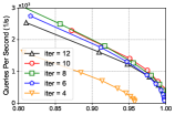
(a) Recall@10 (SIFT1M)

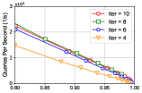
(b) Recall@10 (GIST1M)

Figure 15. Search performance of the benchmark algorithm under different number of iterations.

Table 4 confirms that the highest graph quality does not necessarily achieve the best search performance. Therefore, we set different NN-Descent iteration times to obtain different initial graph quality, so as to get an optimal iteration value of the benchmark algorithm for component evaluation during initialization. As shown in Figure 15, the search performance of the benchmark algorithm with different number of iterations shows the same trend on two real-world datasets. As the number of iterations increases, the search performance first increases and then decreases. This is consistent with the conclusion drawn in Table 4. As far as search performance is concerned, the graph quality is not the higher the better. In addition, according to Table 14, the greater the number of iterations, the higher the index construction time. In summary, we set the number of iterations of NN-Descent to 8 for the benchmark algorithm during initialization.

Table 14. Index construction time (s) of the benchmark algorithm under different number of iterations.

Dataset	iter=4	iter=6	iter=8	iter=10
SIFT1M	164	269	408	532
GIST1M	484	776	1,192	1,721

Appendix M. Index construction performance of components

Table 15 lists the index construction time of the benchmark algorithm using different components.

Table 15. Index construction time (s) of algorithms with different components.

Component	Implementation Way	Dataset
		SIFT1M	GIST1M
C1	C1_NSG	408	1,192
	C1_KGraph	27	90
	C1_EFANNA	64	212
C2	C2_NSSG	408	1,192
	C2_DPG	392	1,179
	C2_NSW	547	1,719
C3	C3_HNSW	408	1,192
	C3_DPG	1,425	22,751
	C3_KGraph	1,065	22,175
	C3_NSSG	1,304	29,164
	C3_Vamana	1,236	24,932
C4 & C6	C4_NSSG	408	1,192
	C4_HCNNG	493	1,465
	C4_IEH	458	1,299
	C4_NGT	432	1,305
	C4_NSG	490	1,472
	C4_SPTAG-BKT	559	1,774
C5	C5_NSG	408	1,192
	C5_Vamana	406	1,261
C7	C7_NSW	408	1,192
	C7_FANNG	449	1,354
	C7_HCNNG	428	1,276
	C7_NGT	399	1,173

Appendix N. Evaluation and analysis of k-DR algorithm

Overview. (Aoyama et al., 2011) presents a fast approximate similarity search method that utilized a degree-reduced k-nearest neighbor graph (k-DR). k-DR first builds a simple KNNG $G(V,E)$, then for any vertex $x$ and its neighbor $y\in N(x)$, k-DR generates an undirected edge between $x$ and $y$ only if the BFS algorithm (Algorithm 1) starting from $y$ cannot find $x$ along the already existing edges on $G$; this is actually an approximation of RNG (similar to NGT, please refer to Appendix B for proof). In addition, k-DR extends the similar range search to NGT (Iwasaki, 2015) for routing.

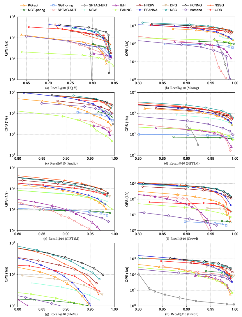
Figure 20. The Queries Per Second (QPS) vs Recall@10 of graph-based ANNS algorithms with their optimal indices in high-precision region on the eight real world datasets (top right is better).

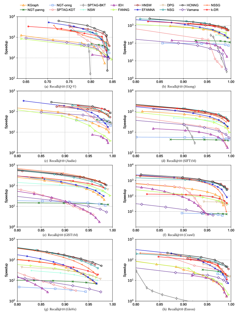
Figure 21. The Speedup vs Recall@10 of graph-based ANNS algorithms with their optimal indices in high-precision region on the eight real world datasets (top right is better).

We analyze the construction and search complexity of k-DR in Appendix D, and summarize some important attributes of k-DR in Table 18. The characteristics of components within k-DR is depicted in Table 9. Appendix H discusses the parameters setting of k-DR. Index construction, search, and scalability performance evaluations are given in Table 11, Table 12, Table 16, Table 17, Figure 20, and Figure 21. In Table 17, GQ, AD, CC, CS, PL, and MO are the abbreviations of graph quality, average out-degree, connected components, candidate set size, query path length, and peak memory overhead respectively.

Table 16. Index construction time (ICT, unit: s) and index size (IS, unit: MB) of k-DR and NGT on real-world datasets, and the bold values are optimal.

Algorithm		UQ-V	Msong	Audio	SIFT1M	GIST1M	Crawl	GloVe	Enron
k-DR	ICT	26,580	36,415	97	15,814	77,917	131,943	27,521	1,416
	IS	66	100	3.6	98	156	171	199	8.4
NGT-panng	ICT	2,094	2,224	51	1,142	5,938	64,507	15,014	236
	IS	215	225	11	229	269	470	312	225
NGT-onng	ICT	3,017	4,814	69	1,989	15,832	174,996	138,348	414
	IS	198	224	9.9	214	296	527	578	21

Table 17. Index and search information of k-DR and NGT on real-world datasets, and the bold values are better.

Algorithm		UQ-V	Msong	Audio	SIFT1M	GIST1M	Crawl	GloVe	Enron
k-DR	GQ	0.574	0.659	0.613	0.647	0.754	0.555	0.747	0.577
	AD	16	25	17	25	40	21	43	22
	CC	19,889	1	1	2	27	10	1	6
	CS	1,440	50	30	130	130	210	210	550
	PL	599	61	29	166	305	2,713	1,402	383
	MO	1,119	1,751	51	657	3,883	2,582	730	516
NGT-panng	GQ	0.770	0.681	0.740	0.762	0.567	0.628	0.589	0.646
	AD	52	56	49	56	67	58	66	55
	CC	1	1	1	1	1	1	1	1
	CS	65	10	10	20	10	10	10	10
	PL	79	144	33	438	1,172	5,132	2,281	83
	MO	1,432	1,927	63	933	4,111	3,111	928	535
NGT-onng	GQ	0.431	0.393	0.412	0.424	0.266	0.203	0.220	0.331
	AD	47	55	45	53	75	66	124	53
	CC	1	1	1	1	1	1	1	1
	CS	1,002	20	15	33	33	157	74	25
	PL	431	227	45	392	1,110	244	388	131
	MO	1,411	2,007	63	859	4,088	3,147	1,331	533

Analysis and discussion. Here we mainly discuss the performance difference between k-DR and NGT due to the similarity of the two. In Table 12, k-DR exceeds NGT on simple dataset by a big margin, however, as the difficulty of the dataset increases, the performance gap between NGT and k-DR gradually narrows. Generally, the scalability of k-DR is better than NGT. As shown in Table 16, the index construction time of NGT is shorter than k-DR, which is mainly because the former initializes an exact KNNG while the initial graph of the latter is approximate. Although k-DR and NGT share the path adjustment strategy, k-DR implements a stricter constraint scheme, while NGT relaxes this constraint. Specifically, once there is an alternative path, k-DR directly deletes the corresponding edge, NGT has to consider the specific situation (Figure 12); this allows k-DR to have a smaller average out-degree, index size and memory overhead. As shown in Table 17, the query path length of k-DR is smaller on some simple datasets, but on some hard datasets, the query path length of NGT is smaller, and NGT-panng has a smaller candidate set size. In addition, the graph quality of k-DR is generally between NGT-onng and NGT-panng, k-DR achieves a better efficiency vs accuracy trade-off than NGT in Figure 20, and Figure 21, which shows too high or too low graph quality does not produce better search performance. In summary, the overall performance of k-DR is better than NGT.

Table 18. Important attributes of k-DR.

Base Graph	Edge	Build Complexity	Search Complexity
KNNG+RNG	undirected	$O(|S|^{2}+k\cdot|S|)$	$O(\log^{5.51}(|S|))$

Appendix O. Trade-off for efficiency vs accuracy

In order to comprehensively evaluate the search performance of each algorithm, their trade-off curves of Queries Per Second (QPS) vs Recall@10 and Speedup vs Recall@10 ared measured on eight real-world datasets in Figure 20 and Figure 21. It is the most important part for the search performance evaluation of graph-based ANNS algorithms as the key of ANNS is seek a good trade-off between efficiency and accuracy. We mainly focus on the performance of each algorithm in the high-precision area due to actual needs (Fu et al., 2019; Fu et al., 2021). On GIST1M, Crawl, and GloVe datasets, SPTAG-BKT falls into the accuracy “ceiling” before reaching Recall@10=0.80, so it is not shown in Figure 20 and Figure 21.

Appendix P. Performance evaluation of the optimized algorithm

We evaluate the performance of the optimized algorithm (OA) and the state-of-the-art algorithms for index construction and search on two real world datasets of different difficulty in the same environment. According to our assessment, OA achieves the best overall performance.

Table 19. Index construction time (s) of the optimized algorithm (OA) and the state-of-the-art algorithms.

Algorithm		OA	NSG	NSSG	HCNNG	HNSW	DPG
Dataset	SIFT1M	1,791	2,503	4,931	8,603	58,526	1,526
	GIST1M	12,440	14,965	13,157	9,934	104,484	6,188

Table 20. Index size (MB) of the optimized algorithm (OA) and the state-of-the-art algorithms.

Algorithm		OA	NSG	NSSG	HCNNG	HNSW	DPG
Dataset	SIFT1M	88	97	80	394	202	293
	GIST1M	79	53	102	326	234	362

Table 21. Graph quality (GQ), average out-degree (AD), and # of connected components (CC) on graph indexes of the optimized algorithm (OA) and the state-of-the-art algorithms.

Algorithm	SIFT1M			GIST1M
	GQ	AD	CC	GQ	AD	CC
OA	0.549	20	1	0.402	18	1
NSG	0.551	24	1	0.402	13	1
NSSG	0.579	20	1	0.399	26	1
HCNNG	0.887	61	1	0.354	42	1
HNSW	0.879	49	22	0.633	57	122
DPG	0.998	76	1	0.992	94	1

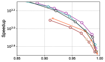
(a) Recall@10 (Msong)

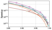
(b) Recall@10 (SIFT1M)

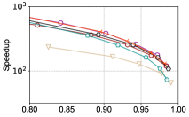
(c) Recall@10 (GIST1M)

Figure 16. The Speedup vs Recall@10 of the optimized algorithm (OA) and the state-of-the-art algorithms. (top right is better).

Table 22. Candidate set size (CS), query path length (PL), and peak memory overhead (MO) of the optimized algorithm (OA) and the state-of-the-art algorithms.

Algorithm	SIFT1M			GIST1M
	CS	PL	MO	CS	PL	MO
OA	99	95	682	266	380	3,846
NSG	101	85	653	867	826	3,781
NSSG	255	157	640	280	270	3,829
HCNNG	97	37	1,056	371	179	4,159
HNSW	66	47	1,206	181	130	4,372
DPG	37	30	851	55	124	4,091

Index construction performance. As shown in Table 19, Table 20 and Table 21, compared with the state-of-the-art algorithms, the index construction efficiency of the optimized algorithm (OA) ranks very high (second only to DPG, but OA performs better than DPG in other aspects), which is mainly because OA is not committed to achieving high graph quality at an expensive time cost (Table 21), and its neighbor acquisition does not involve distance calculation. There is no additional structure attached to the graph index for OA, which makes it obtain a smaller index size; and that is also due to its smaller average out-degree. In addition, OA ensures the accessibility from the entries to any other point, which is backed up by the number of connected components.

Search performance. As shown in Figure 16, OA obtains the optimal speedup vs recall trade-off on SIFT1M and GIST1M. At the same time, its candidate set size, query path length, and peak memory overhead are all close to the optimal values in Table 22.

Appendix Q. Multiple trials for randomized parts of the algorithms

Table 23. Index construction time (ICT, unit: s) and index size (IS, unit: MB) of Vamana under different trails (a, b, and c).

Trial		UQ-V	Msong	Audio	SIFT1M
ICT	a	1,451	1,786	158	2,657
	b	1,575	1,736	145	2,756
	c	1,378	1,695	139	2,608
	Average	1,468	1,739	147	2,674
IS	a	119	118	11	195
	b	119	118	11	195
	c	119	118	11	195
	Average	119	118	11	195

For some algorithms that include the randomization, we perform multiple experiments under the same environment and report the average value. According to our experimental results in Table 23, Figure 17 and Figure 18, we conclude that a single value is very close to the average value. Below we take Vamana and NSSG as examples to explain the reasons for the above phenomenon.

Vamana. The initialization of the graph index is to randomly select a given number of neighbors for each element on the dataset. For the convenience of description, we divide any vertex’s neighbors to “good neighbors” (GN) and “bad neighbors” (BN). If we initialize GN for each vertex, Vamana’s index construction efficiency can reach the optimal value, as GN enable Vamana to perform ANNS more efficiently when acquiring candidate neighbors. In contrast, if BN are initialized for each element, it will lead to the worst index construction efficiency. However, the probability of the above two situations happening is extremely low (close to zero). Actually, the ratio of GN and BN of each element is relatively stable. In general, Vamana’s ANNS performance with different initial graphs is close (see Figure 17). When ignoring the cost of neighbor selection (it does not affected by the initial graph), its index construction efficiency mainly depends on ANNS on the initial graph for obtaining candidate neighbors; so it is almost the same under different trails.

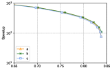
(a) Recall@10 (UQ-V)

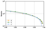
(b) Recall@10 (Msong)

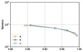
(c) Recall@10 (Audio)

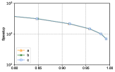
(d) Recall@10 (SIFT1M)

Figure 17. Speedup vs Recall@10 of Vamana under different trails (a, b, and c).

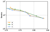
(a) Recall@10 (UQ-V)

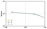
(b) Recall@10 (Msong)

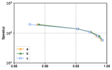
(c) Recall@10 (Audio)

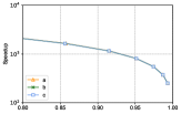
(d) Recall@10 (SIFT1M)

Figure 18. Speedup vs Recall@10 of NSSG under different trails (a, b, and c).

NSSG. The seed acquisition component of NSSG is randomized. As shown in Figure 18, the search performance curves of NSSG under different experiments almost overlap. For the convenience of description, we also divide the seeds into “good seeds” (GS) and “bad seeds” (BS). Performing search from GS can get the best search performance, while starting search from BS will result in the worst search performance. Due to the sufficient amount of query data (¿ 200, Table 3), the probability that the randomly obtained seeds is GS or BS for all queries is almost zero; for a given batch of queries, the ratio of the two is stable. Therefore, random seeds with multiple repetitions produce similar search performance.

Appendix R. Evaluation and analysis of machine learn (ML) based methods

Overview. In general, ML-based approaches append additional optimizations on existing graph-based algorithms. For example, (Baranchuk et al., 2019) (ML1) learns vertex representation on graph-based algorithms (e.g., NSW) to provide a better routing; (Li et al., 2020) (ML2) performs ANNS on HNSW through learned adaptive early termination, it builds and trains gradient boosting decision tree models to learn and predict when to stop searching for a certain query; (Prokhorenkova and Shekhovtsov, 2020) (ML3) maps the dataset into a space of lower dimension while trying to preserve local geometry by ML, then it can be combined with any graph-based algorithms like HNSW or NSG.

Setting. We implement ML1 and ML3 optimization on NSG, and implement ML2 optimization on HNSW (HNSW is selected in the original paper (Li et al., 2020)); considering that when ML2 is applied to NSG, some additional optimization is required (we will add ML2 to NSG soon for evaluation after solving these problems). We focus on the index processing time, memory consumption during index construction, and speedup vs recall trade-off of each method. Note that ML1’s index preprocessing training is very time-consuming and memory-consuming (more than 125G on SIFT1M), so we use GPU to accelerate the process and use the smaller SIFT100K and GIST100K datasets. In addition, the number of nearest neighbors recalled is uniformly set to 1 for each query due to the limitation of ML1 (Baranchuk et al., 2019), and Recall@1 represents the corresponding recall rate.

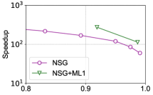
(a) Recall@1 (SIFT100K)

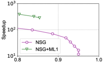
(b) Recall@1 (GIST100K)

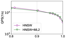
(c) Recall@1 (SIFT100K)

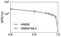
(d) Recall@1 (GIST100K)

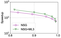
(e) Recall@1 (SIFT100K)

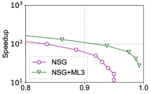
(f) Recall@1 (GIST100K)

Figure 19. Speedup vs Recall@10 of ML-based methods.

Table 24. Index processing time (IPT) and memory consumption (MC) of ML-based methods.

Method		SIFT100K	GIST100K
IPT(s)	NSG	55	142
	NSG+ML1	67,315	45,742
	HNSW+ML2	2,018	2,626
	NSG+ML3	1,260	1,287
MC(GB)	NSG	0.37	0.68
	NSG+ML1	23.8	58.7
	HNSW+ML2	3	5.7
	NSG+ML3	23	25.5

Discussion. As shown in Table 24 and Figure 19, there ML-based optimizations generally obtain better speedup (or QPS) vs recall tradeoff than the original algorithms (NSG or HNSW) at the expense of more time and memory. ML2 only provides slight latency reduction in the high-precision area. It is worth noting that ML2 have a smaller impact on IPT and IS (compared to HNSW). The IPT of ML1 is significantly higher than the original NSG, and it also requires additional index overhead. Although ML3 improves the speedup vs recall tradeoff by a large margin, it also significantly increases memory consumption.