Phases of Holographic Interfaces

Abstract

We compute the phase diagram of the simplest holographic bottom-up model of conformal interfaces. The model consists of a thin domain wall between three-dimensional Anti-de Sitter (AdS) vacua, anchored on a boundary circle. We distinguish five phases depending on the existence of a black hole, the intersection of its horizon with the wall, and the fate of inertial observers. We show that, like the Hawking-Page phase transition, the capture of the wall by the horizon is also a first order transition and comment on its field-theory interpretation. The static solutions of the domain-wall equations include gravitational avatars of the Faraday cage, black holes with negative specific heat, and an intriguing phenomenon of suspended vacuum bubbles corresponding to an exotic interface/anti-interface fusion. Part of our analysis overlaps with recent work by Simidzija and Van Raamsdonk but the interpretation is different.

$\,{}^{1}$ Laboratoire de Physique de l’École Normale Supérieure,
CNRS, PSL Research University and Sorbonne Universités
24 rue Lhomond, 75005 Paris, France

1 Introduction

Begining with the classic paper of Coleman and De Lucia [1] there have been many studies of thin gravitating domain walls between vacua with different values of the cosmological constant. Such walls figure in models of localized gravity [2, 3, 4], in holographic duals of conformal interfaces [5, 6, 7], in efforts to embed inflation in string theory by studying dynamical bubbles [8, 9, 10, 11], and more recently, following the ideas in refs. [12, 13, 14], in toy models of black hole evaporation [15, 16, 17, 19, 18, 20, 21, 22, 23]. Besides being a simple form of matter coupled to gravity, domain walls are also a key ingredient [24] in effective descriptions of the string-theory landscape – see [25, 26, 27] for some recent discussions of domain walls in this context.

In this paper we study a thin static domain wall between Anti-de Sitter (AdS) vacua, anchored at the conformal boundary of spacetime. If a dual holographic setup were to exist, it would have two conformal field theories, CFT₁ and CFT₂, separated by a conformal interface [5, 6, 7]. We will calculate the phase diagram of the system as function of the AdS radii, the tension of the wall and the boundary data. Several parts of this analysis have appeared before (see below) but the complete phase diagram has not, to the best of our knowledge, been worked out. We will be interested in phenomena that are hard to see at weak CFT coupling. A broader motivation, as in much of the AdS/CFT literature, is understanding how the interior geometry is encoded on the boundary and vice versa, but we will only briefly allude to this question in the present work.

Our analysis is classical in gravity. Different phases are distinguished by the presence/absence of a black hole and by the fate of inertial observers, either those moving freely in the bulk or those bound to the wall. Inertial observers are a guiding fixture of the analysis, not emphasized in earlier works. In the high-temperature or ‘hot’ phase all inertial observers eventually cross the black-hole horizon. In intermediate or ‘warm’ phases the wall avoids the horizon, and may also shield bulk observers from falling inside. Such two-center warm solutions are gravitational avatars of the Faraday cage. Finally what differentiates ‘cold’ horizonless phases is whether all timelike geodesics intersect inevitably the wall, or not.

Besides the domain wall and the black hole, the third actor in the problem is the center of global AdS where an inertial observer may rest. The rich phase diagram is the result of several competing forces: The attraction of the AdS trap, with or without a black hole in its center, the tension of the wall, and the repulsion between the domain wall and massive particles. In addition to the first-order Hawking-Page transition [28] that signals the formation of a black hole, new phase transitions occur when the wall sweeps an AdS rest point or when part of it enters the horizon, see figure 1. One of our conclusions is that the latter transition is always first-order.

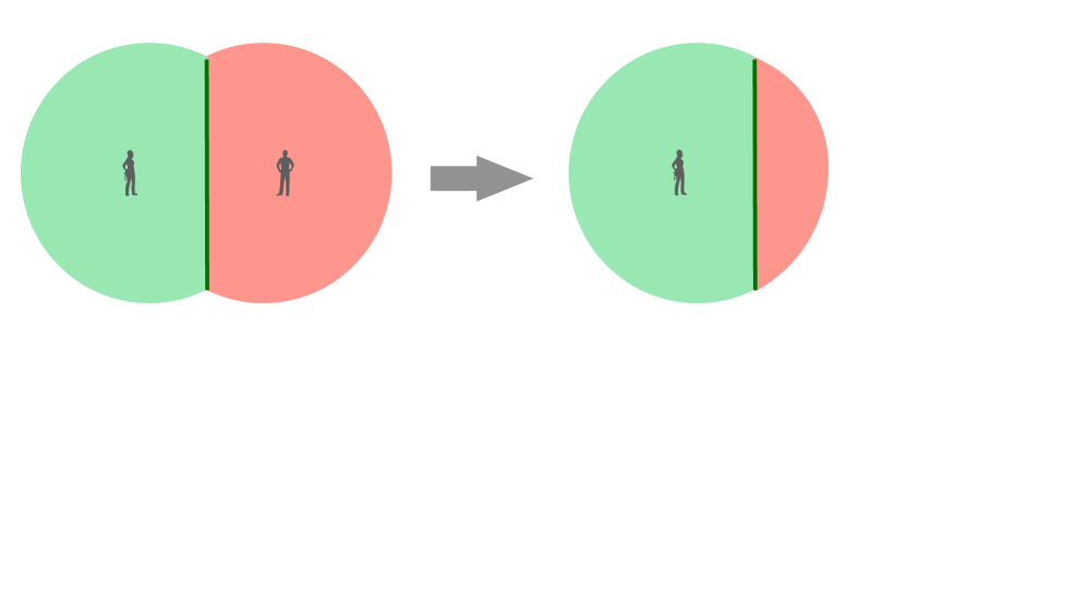
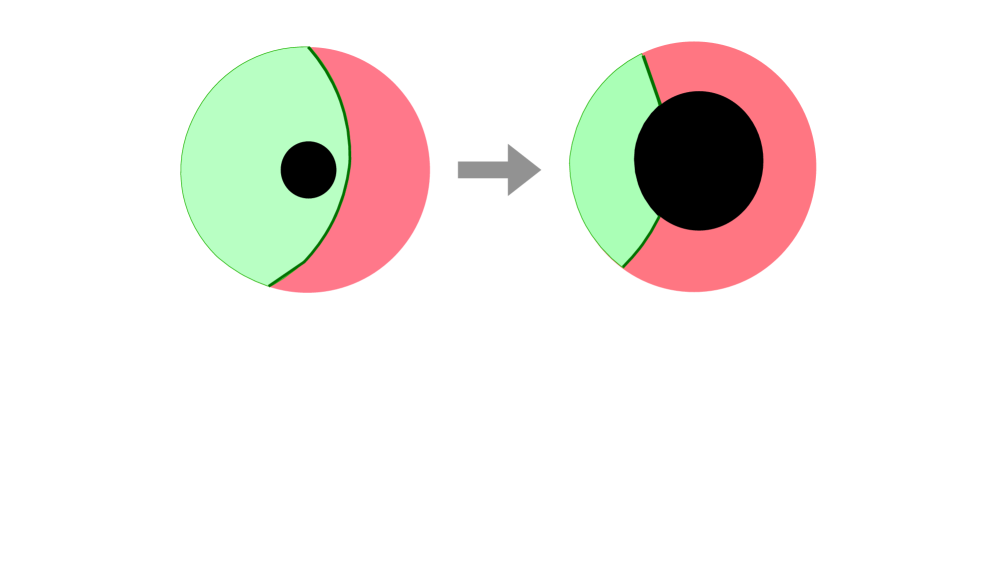
Figure 1: A domain wall sweeping the center of the ‘false AdS vacuum’ where an inertial observer could rest (left), or entering the horizon of a black hole (right).

We work in 2+1 dimensions because calculations can be performed in closed form. We expect, however, qualitative features of the phase diagram to carry over to higher dimensions. For simplicity we consider a single type of non-intersecting wall, and only comment briefly on extended models that allow junctions of different types of wall.

The capture of the wall by the black hole is related to a transition analyzed in a very interesting recent paper by Simidzija and Van Raamsdonk [29], see also [30, 31]. These authors consider time-dependent spherically-symmetric walls whose intersections with the conformal boundary describe Hamiltonian quenches in the dual field theory. In this setting the boundary is the infinite cylinder, with a stripe describing the evolution of the dual CFT between the quench and ‘unquench’ times. By contrast, we are interested in equilibrium configurations. This means that the domain-wall geometry is static, and the stripes on the conformal boundary point in the time direction. Furthermore, the boundary is not the cylinder but an orthogonal torus, adding an extra parameter to the problem.

Although the interpretation is different, many of our formulae are nevertheless related to those of refs. [30, 29, 31] by swapping the roles of boundary space and time (thereby also swapping the BTZ geometry with thermal AdS₃, see section 2). This is fortuitous to 2+1 dimensions and does not carry over to higher dimensions.

The gravitational action of the thin-wall model reads

$$\,\hskip-42.67912ptI_{\rm gr}=-\frac{1}{2}\int_{{\mathbb{S}}_{1}}d^{3}x\sqrt{g_{1}}\,(R_{1}+\frac{2}{\ell_{1}^{2}})\hskip-5.69054pt - \hskip-5.69054pt\frac{1}{2}\int_{{\mathbb{S}}_{2}}d^{3}x\sqrt{g_{2}}\,(R_{2}+\frac{2}{\ell_{2}^{2}})$$ (1.1)

$$\hskip-51.21495pt+\,\lambda\int_{\mathbb{W}}d^{2}s\sqrt{\hat{g}_{w}}\,+\,{\rm GHY\ terms}\,+\,{\rm ct.}\ ,\$$

where $R_{j}(g_{j})$ are the Ricci scalars of the spacetime slices $\mathbb{S}_{j}$ on either side of the wall, and $\hat{g}_{w}$ is the induced metric on the wall’s worldvolume. The Gibbons-Hawking-York terms and counterterms are given in appendix A. The action $I_{\rm gr}$ depends on three parameters: the two AdS radii $\ell_{1},\ell_{2}$ and the wall tension $\lambda$. The radii are related to the central charges of the dual CFTs [32], and the tension to the entropy [33, 29] and to the energy-transport coefficient [34] of the dual interface. Static solutions exist for

$$\lambda_{\rm min}<\lambda<\lambda_{\rm max}\,,\qquad{\rm with}\quad\lambda_{\rm max}={1\over\ell_{1}}+{1\over\ell_{2}}\,;\ \ \lambda_{\rm min}=\bigl{|}{1\over\ell_{1}}-{1\over\ell_{2}}\bigr{|}\ .$$ (1.2)

The classical phase diagram depends on two dimensionless ratios of the above (e.g. $\ell_{2}/\ell_{1}:=b\,$ and $\lambda\ell_{2}:=\kappa$) and on the two parameters that determine the conformal class of the striped boundary torus, e.g. $\tau_{1}:=TL_{1}$ and $\tau_{2}:=TL_{2}$, see figure 2. Without loss of generality we assume henceforth that $\ell_{2}\geq\ell_{1}$, i.e. that $\mathbb{S}_{1}$ is the true-vacuum slice.

An important question is how much of this analysis has a chance to carry over to top-down holographic models, where back-reacting domain walls are not thin. The size of the horizon and the number of stable rest points are order parameters that can be also defined for thick walls, but a sharp criterion, that decides whether a thick domain wall enters or avoids the horizon is hard to imagine. Nevertheless, the field-theory interpretation of the transition suggests that such an order parameter may exist, as we will explain in section 7.1.

It is worth stressing that the thin-wall model is a minimal gravity dual of I(nterface) CFT in the same way that pure Einstein theory is a minimal dual for homogeneous CFT. The model captures the two universal boundary operators – the energy-momentum tensors on either side of the interface, as well as their combination refered to as the displacement operator [54]. Top-down models have many more operators, some of which correspond to internal excitations of the domain wall.

Note also that boundaries, or end-of-the-world branes (EWBs), can be considered as a limit of domain walls when one side becomes the zero-radius AdS spacetime [55]. In this sense holographic B(oundary) CFT [56, 57] can be recovered from holographic ICFT, though the limit is subtle and should be handled with care.

A last remark concerns the Ryu-Takayanagi surfaces [58, 59] that delimit the entanglement wedges of boundary subregions [60, 62, 61]. It is clearly of interest to study if these surfaces intersect the domain wall, as is done for BCFT in ref. [21, 22]. We hope to return to this question elsewhere.

The plan of the paper and a summary of our results follows. In section 2 we review some standard facts about AdS₃/CFT₂ at finite temperature. The wall separates space in two slices that we color green (true-vacuum side) and pink (false-vacuum side). Each of these comes in one of four topological types described in section 3. In section 4 we solve the matching equations obeyed by a thin static domain wall, which we parametrize conveniently by the blueshift metric factor $g_{tt}$. This section overlaps substantially with ref. [29] via double Wick rotation – a trick specific to 2+1 dimensions as earlier noted.

In section 5 we start analyzing the solutions. By studying the turning point of the wall we classify the possible phases, i.e. the topologically distinct solutions. We rule out in particular centerless geometries, in which no inertial observer can avoid the wall, and solutions with two black holes whose merging is prevented by the wall.

In section 6 we write down the equations of state that characterize these phases. They relate the canonical variables $\tau_{1},\tau_{2}$ to microcanonical variables that are natural for describing the interior geometry. We also point out the relevance of a critical tension $\lambda_{0}=\sqrt{\lambda_{\rm max}\lambda_{\rm min}}\,$ below which the hot solution disappears from a region of parameter space.

In section 7 we compute the critical lines for sweeping transitions in both the cold and the warm phases, and we show that the warm-to-hot transition is always first-order – the domain wall cannot be lowered continuously to the black horizon. The proof requires a detailed analysis of the region $\mu\approx 1$ with $\lambda\leq\lambda_{0}$, where the hot and a warm solution come arbitrarily close. We also point out some puzzles regarding the ICFT interpretation of these phase transitions.

Section 8 presents a striking phenomenon: bubbles of the true vacuum suspended from a point on the conformal boundary of the false vacuum. This is surprising from the perspective of ICFT, since it implies that the fusion of an interface and anti-interface does not produce the trivial (identity) defect, as expected from free-field calculations [65], but an exotic defect that generates spontaneously a new scale.

In section 9 we present numerical plots of the complete phase diagram in the canonical ensemble, for different values of the Lagrangian parameters $\lambda,\ell_{j}$. These plots confirm our earlier conclusions. We point out a critical threshold $b=\ell_{2}/\ell_{1}=3$, probably an artifact of the thin-wall approximation, above which black-hole solutions on the false-vacuum side of the wall cease to exist. We also exhibit coexisting black-hole solutions, including black holes with negative specific heat. This parallels the discussion of black holes in deformed JT gravity in ref. [66].

Section 10 contains concluding remarks. In order not to interrupt the flow of the arguments we relegate some detailed calculations to four appendices.

2 Finite-temperature AdS/CFT

For completeness we recall here some standard facts about AdS/CFT at finite temperature in three spacetime dimensions. While doing this we will be also setting notation and conventions.

2.1 Coordinates for the AdS₃ black string

The metric of the static AdS₃ black string in 2+1 dimensions is

$$ds^{2}_{\rm BS}\,=\,{\ell^{2}dr^{2}\over r^{2}-M\ell^{2}}-({r^{2}}-M\ell^{2})\,dt^{2}+r^{2}dx^{2}\,,$$ (2.1)

where $M>0$, $\ell$  is the radius of AdS₃ and the horizon at $r^{\rm H}=\ell\sqrt{M}$ has temperature $T=\sqrt{M}/2\pi$. Length units on the gravity side are such that $8\pi G=1$. The dual CFT lives on the AdS₃ boundary, at $r={1/\epsilon}\to\infty$, with conformal coordinates  $x^{\pm}\equiv x\pm t\,\in\mathbb{R}^{2}$. Its central charge is $c=12\pi\ell$ [32].

The holographic dictionary becomes transparent in Fefferman-Graham coordinates, in which any asymptotically-Poincaré AdS₃ solution takes the following form [67, 68]

$$ds^{2}={\ell^{2}dz^{2}\over z^{2}}+{1\over z^{2}}\Bigl{(}dx^{+}+{\ell z^{2}}h_{-}dx^{-}\Bigr{)}\Bigl{(}dx^{-}+{\ell z^{2}}h_{+}dx^{+}\Bigr{)}\ .$$ (2.2)

Here $h_{\pm}=\langle T_{\pm\pm}\rangle$ are the expectation values of the canonically-normalized energy-momentum tensor of the CFT. Note that it is a special feature of 2+1 dimensions that the Fefferman-Graham expansion stops at order $z^{2}$. For the static black string, $h_{+}=h_{-}=M\ell/4\,$ giving $\langle T_{tt}\rangle=M\ell/2=(c/6)\pi T^{2}$. This is indeed the energy density of finite-temperature CFT in two dimensions. The relation between $z$ and $r$ is

$${r}={1\over z}+{M\ell^{2}z\over 4}\ \ \Longleftrightarrow\ \ z={2\over M\ell^{2}}\left(r-\sqrt{{r^{2}}-M\ell^{2}}\,\right)\ ,$$ (2.3)

and the black-string metric in the $(z,t,x)$ coordinates reads

$$ds^{2}_{\rm BS}\,=\,\ell^{2}{dz^{2}\over z^{2}}-\Bigl{(}{1\over z}-{M\ell^{2}z\over 4}\Bigr{)}^{2}dt^{2}+\Bigl{(}{1\over z}+{M\ell^{2}z\over 4}\Bigr{)}^{2}dx^{2}\ .$$ (2.4)

Note that $z$ covers only the region outside the horizon ($r>r^{\rm H}$) and that near the conformal boundary $z\approx r^{-1}$.

A last change of coordinates worth recording, even though we will not use it in this paper, is the one that maps $(z,t,x)$ to the standard Poincaré parametrization of AdS₃. Such a map is guaranteed to exist because all constant-negative-curvature Einstein manifolds in three dimensions can be obtained from AdS₃ by identifications and excisions. For the case at hand  the transformation reads

$$w^{\pm}=\zeta^{\pm}\left({4-M\ell^{2}z^{2}\over 4+M\ell^{2}z^{2}}\right)\,,\quad y={4z(M\zeta^{+}\zeta^{-})^{1/2}\over 4+M\ell^{2}z^{2}}\quad{\rm with}\quad\zeta^{\pm}=e^{\sqrt{M}(x\pm t)}\ .\ \$$ (2.5)

The reader can check that in these coordinates the metric (2.4) becomes

$$ds^{2}_{\rm BS}\,=\,{\ell^{2}dy^{2}+dw^{+}dw^{-}\over y^{2}}\ ,$$ (2.6)

i.e. the standard Poincaré form of AdS₃ as advertized. Outside the black horizon ($M\ell^{2}z^{2}<4$) the coordinates $x^{\pm}\equiv x\pm t$ cover only a Rindler wedge of the $w^{\pm}$ plane.

Since we will be refering to this later, let us verify the well-known fact that no inertial observer can avoid crossing the horizon. In the proper-time parametrization of the trajectory a simple calculation gives

$$\ell^{2}\,{{\ddot{r}}\over r}=-1-M\ell^{2}{\dot{x}}^{2}$$ (2.7)

where dots denote derivatives with respect to proper time. Since $M$ is positive there is no centrifugal acceleration QED. Note that this is a property of the asymptotically AdS black hole, not shared by asymptotically flat black holes in higher dimension.

2.2 Hawking-Page transition

From the perspective of the CFT, the temperature $T$ is the only dimensionful parameter of the infinite-black-string solution. By a scale transformation we can always set it to one. Things get more interesting if the black string is compactified, $x\sim x+L$, thereby converting the solution (2.1) to the non-spinning BTZ black hole [72, 73]. In addition to the central charge $c$, there is now a new dimensionless parameter $LT$. In the Euclidean geometry $\tau=i\,LT$ is the complex-structure modulus of the boundary torus.

At the critical temperature $T_{\rm HP}=1/L$ the theory undergoes a Hawking-Page phase transition [28, 74]. This is seen by comparing the action of the two competing saddle points for the interior geometry:  (i) the Euclidean BTZ black hole, and (ii) thermal AdS₃, whose metric is the same as (2.1) but with $M$ replaced by $\tilde{M}=-(2\pi/L)^{2}$. The difference of free energies of these two saddle points reads

$$F_{\rm BTZ}-F_{\rm TAdS}=-2\pi^{2}\ell\,\bigl{(}LT^{2}-{1\over L}\bigr{)}\ .$$ (2.8)

Thus thermal AdS₃ is the dominant solution when $LT<1$, while the BTZ black hole dominates when $LT>1$.

Thermal AdS₃ and the Euclidean BTZ black hole differ in the choice of boundary cycle that becomes contractible in the interior geometry. The periodicity conditions, respectively $x\sim x+2\pi/|\tilde{M}|^{1/2}$ and $t_{E}\sim t_{E}+2\pi/M^{1/2}$, ensure regularity when this contractible cycle degenerates. Below we will encounter situations in which either the center of AdS or the BTZ horizon are excised. In such cases the regularity conditions can be relaxed.

One other comment in order here concerns the difference of free energies, eq. (2.8). The renormalized gravitational action $I_{\rm gr}$ (where $I_{\rm gr}=F/T$) is calculated for the general interface model in appendix A. In the case of a homogeneous CFT one can, however, obtain the answer faster. Indeed, from the Fefferman-Graham form of the metric, eq. (2.2), one reads the energy of the CFT state,

$$E=\,L\langle T_{tt}\rangle\,=\,{1\over 2}\ell ML\ .$$ (2.9)

For $M=(2\pi T)^{2}$ this is the internal energy of the high-temperature state, as previously noted, and for $M=-(2\pi/L)^{2}$ it is the Casimir energy of the vacuum. The corresponding free energies obey the thermodynamic identity

$$E=-T^{2}{\partial\over\partial T}\Bigr{(}{F\over T}\Bigl{)}\ .$$ (2.10)

Eqs. (2.9) and (2.10) determine $F$ up to a term linear in $T$. This can be argued to vanish both at low $T$, since the ground state has no entropy, and at large $L$ since $F$ must be extensive. The final result is eq. (2.8).

Let us finally note that since in empty AdS the mass $M$ is negative, there is a centrifugal contribution in eq.(2.7). An inertial observer may thus either rest at, or orbit around the center $r=0$. But in the centerless slices that we are about to discuss, all inertial observers hit the wall.

3 Topology of slices

Consider now two conformal field theories, CFT₁ and CFT₂, coexisting at thermal equlibrium on a circle. This is illustrated in figure 1. The horizontal and vertical axes parametrize space and Euclidean time. In addition to the central charges $c_{1},c_{2}$, and to the properties of the interfaces between the two CFTs, there are three more parameters in this system: the sizes $L_{1},L_{2}$ of the regions in which each CFT lives, and the equilibrium temperature $T$. This gives two dimensionless parameters, which we can choose for instance to be $\tau_{1}:=TL_{1}$ and $\tau_{2}:=TL_{2}$.

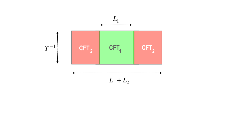
Figure 2: The finite-temperature interface CFT at the AdS boundary. Both space and Euclidean time are compact, so the depicted surface is an orthogonal torus.

The gravity dual of this ICFT features domain walls, i.e. strings in 2+1 dimensions,  anchored at the interfaces on the conformal boundary. We will make the simplifying assumption that the two domain walls differ only in orientation, and can join smoothly in the interior of spacetime. Extended models allowing junctions of different domain walls are very interesting but they are beyond our present scope. We will comment briefly on them in a later section.

The green and pink boundary regions of fig. 2, in which CFT₁ and CFT₂ live, extend in the interior to slices of gravitational solutions that belong to one of several topological types. These are illustrated for the green slice in figure 3. Each slice is either part of thermal AdS₃ with the center, marked by a grey flag, included (E1) or excised (E2), or part of the BTZ geometry with the horizon excised (E2^′), included (H1) or intersecting the domain wall (H2). The same options are available for the pink spacetime slice.

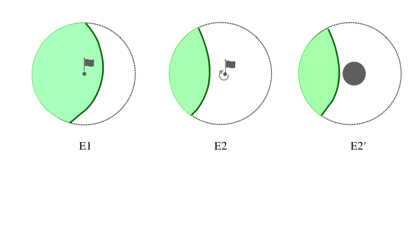
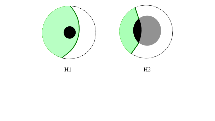
Figure 3: The different types of space-time slice described in the main text. The actual slice is colored in green, the complementary region is excised. The letters ‘E’ and ‘H’ stand for ‘empty’ and ‘horizon’, and the grey flag denotes the rest point of an inertial observer. Note that since this is excised in E2, a conical singularity in its place is permitted. The centerful slice E1 can act as a gravitational Faraday cage.

As was explained in section 2, we may adopt the unified parametrization (2.1) for all types of slice, with $M$ negative for the slices of type E1 and E2  of global AdS₃, and positive for the slices of type E2^′, H1 and H2 of the BTZ spacetime. We are interested in static configurations which are dual to equilibrium CFT states, so time is globally defined and has fixed imaginary period $t_{E}\sim t_{E}+1/T$. The coordinates $(x,r)$ on the other hand need not be continuous across the wall. We therefore write the spacetime metric in terms of two coordinate charts,

$$ds^{2}\,=\,{\ell_{j}^{2}dr_{j}^{2}\over r_{j}^{2}-M_{j}\ell_{j}^{2}}-({r_{j}^{2}}-M_{j}\ell_{j}^{2})\,dt^{2}+r_{j}^{2}dx_{j}^{2}\qquad{\rm with}\quad(x_{j},r_{j})\in\Omega_{j}\,,\,\,$$ (3.1)

where $\Omega_{1}$ is the range of coordinates for the green slice and $\Omega_{2}$ the range of coordinates for the pink slice. These ranges are delimited as follows:

• by the embeddings of the static wall in the two coordinate systems, $\{x_{j}(\sigma),r_{j}(\sigma)\}$, where $\sigma$ parametrizes the wall ;

• by the horizon whenever the slice contains one, i.e.  in cases H1 and H2 ;

• by the cutoff surface $r_{j}\approx 1/\epsilon\to\infty$  .

The mass parameters of the slices, $M_{1}$ and $M_{2}$, are in general different. Regularity requires however that

$$M_{j}=(2\pi T)^{2}\qquad{\text{for\ slices\ \ {\small{H1, H2}}}}$$ (3.2)

that include a horizon, whereas $M_{j}$ is unconstrained for the other slice types. Furthermore, for a slice of type E1 in which the spatial circle is contractible, interior regularity fixes the periodicity of $x$,

$$x_{j}\sim x_{j}+2\pi/\sqrt{-M_{j}}\qquad{\text{ in\ case\ {\small E1}}}\ .$$ (3.3)

For E2, E2^′ and H2 the coordinate $x_{j}$ is not periodic, while for H1 its period, proportional to the horizon size, is unconstrained.

Since the horizon is a closed surface, a green slice of type H2 can only be paired with a pink slice of the same type. This is the topology that dominates at very high temperature when the black hole eats up most of the bulk spacetime. As the temperature is lowered different pairs of the remaining slice types dominate. The pairs that correspond to actual solutions of the domain-wall equations will be determined in section 5.

For the time being let us comment on the differences between the horizonless slices in the top row of fig. 3. What distinguishes E1 from the other two is the existence of the AdS center (or ‘refuge’) where an inertial observer may sit at rest. By contrast, in the slices of type E2 and E2^′ all inertial observers will inevitably hit the domain wall as explained in the previous subsection. This discontinuous behavior differentiates the phases on either side of a sweeping transition.

Note that there is no topological difference between the slices of type E2 and E2^′, which is why we distinguish them only by a prime. These slices differ only in the sign of $M_{j}$, or equivalently the energy density per degree of freedom in the boundary theory. Together E2 and E2^′ describe a continuum ($-\infty<M_{j}<\infty$) of horizonless slices with no rest point.

4 Solving the wall equations

In this section we find the general solution of the domain wall equations in terms of the mass parameters $M_{1},M_{2}$, the AdS radii $\ell_{1},\ell_{2}$, and the tension of the wall $\lambda$. That a solution always exists for any bulk geometries is a special feature of 2+1 dimensions, as is the double Wick rotation that relates this part of our analysis to ref. [29].

4.1 Matching conditions

The matching conditions at a thin domain wall have appeared in numerous studies of cosmology and AdS/CFT. They are especially simple in the case at hand, where the wall/string is static and is characterized only by its tension. Matching the induced worldsheet metric of the two charts (3.1) gives one algebraic and one first-order differential equation for the embedding functions $x_{1}(\sigma),r_{1}(\sigma),x_{2}(\sigma)$ and $r_{2}(\sigma)$:

$${r_{1}^{2}}-M_{1}\ell_{1}^{2}\,=\,{r_{2}^{2}}-M_{2}\ell_{2}^{2}\,\,\equiv\,f(\sigma)$$ (4.1)

$${\rm and}\qquad\ \ f^{-1}{\ell_{1}^{2}\,r_{1}^{\prime\,2}}+r_{1}^{2}\,x_{1}^{\prime\,2}=f^{-1}{\ell_{2}^{2}\,r_{2}^{\prime\,2}}+r_{2}^{2}\,x_{2}^{\prime\,2}\,\equiv\,g(\sigma),$$ (4.2)

where the prime denotes a derivative with respect to $\sigma$. We have defined the auxiliary functions $f$ and $g$ in terms of which the induced worldsheet metric reads $d{\hat{s}}^{2}|_{\mathbb{W}}=-f(\sigma)dt^{2}+g(\sigma)d\sigma^{2}$. A third matching equation expresses the discontinuity of the extrinsic curvature in terms of the tension, $\lambda$, of the wall [76, 77]. It can be written as follows :

$${r_{1}^{2}x_{1}^{\prime}\over\ell_{1}}+{r_{2}^{2}x_{2}^{\prime}\over\ell_{2}}=\lambda\,\sqrt{fg}\ .$$ (4.3)

Our convention is that $\sigma$ increases as one circles $\Omega_{j}$ in the $(x_{j},r_{j})$ plane clockwise. Other conventions introduce signs in front of the two terms on the left-hand side of this equation.

Eqs. (4.1)–(4.3) are three equations for four unknown functions, but one of these functions can be specified at will using the string-reparametrization freedom. Furthermore the equations only involve first derivatives of $x_{j}$, so the integration constants are irrelevant choices of the origin of the $x_{j}$ axes. For given $\ell_{1},\ell_{2}$ and $\lambda$, the wall embedding functions $x_{j}(r_{j})$, are thus uniquely determined by the parameteres $M_{1}$ and $M_{2}$. Different choices of ($M_{1},M_{2}$) may correspond, however, to the same boundary data ($L_{1},L_{2},T$). These are the competing phases of the system.

4.2 Solution near the boundary

Near the conformal boundary, $r_{j}\to\infty$, the parameters $M_{j}$ can be neglected and the worldsheet metric asymptotes to AdS₂ by virtue of scale invariance. Explicitly the solution reads [78]

$$r_{1}\approx r_{2}\,,\qquad x_{j}\,\approx\,-\ell_{j}\,(\tan\theta_{j})\,r_{j}^{-1}\ ,$$ (4.4)

where $\theta_{j}$ is the angle in the $(x_{j}\,,\ell_{j}/r_{j})$ plane between the normal to the boundary and the interface, see figure 4. The matching eqs. (4.2) and (4.3) relate these angles to the bulk radii $\ell_{j}$ and to the string tension $\lambda$:

$${\ell_{1}\over\cos\theta_{1}}={\ell_{2}\over\cos\theta_{2}}\,\equiv\,\ell_{w}\qquad{\rm and}\qquad\tan\theta_{1}+\tan\theta_{2}=\,{\lambda}\,\ell_{w}\ ,$$ (4.5)

where $\ell_{w}$ is the radius of the AdS₂ worldsheet, and $-{\pi/2}<\theta_{j}<{\pi/2}$ .

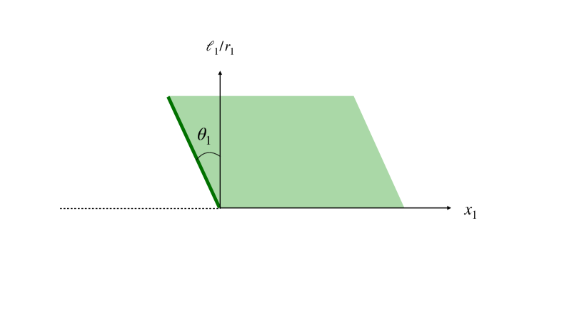
Figure 4: Near the AdS boundary in the $(x_{j},\ell_{j}/r_{j})$ plane the string is a straight line subtending an angle $\theta_{j}$ with the normal.

Without loss of generality we assume that $\ell_{1}\leq\ell_{2}$, so that CFT₁ has the smaller of the two central charges. Its gravity dual has the lower vacuum energy, i.e. the green slice is the ‘true vacuum’ side of the domain wall and the pink slice is the ‘false-vacuum’ side. The first eq. (4.5) then implies that $|\tan\theta_{1}|\geq|\tan\theta_{2}|$  and, provided that the tension is positive, the second eq. (4.5) implies that $\theta_{1}>0$. The sign of $\theta_{2}$, on the other hand, depends on the precise value of $\lambda$. Expressing the tangents in terms of cosines brings indeed this equation to the form

$$({1\over\ell_{1}^{\,2}}-{1\over\ell_{w}^{\,2}})^{1/2}\,+\,\varepsilon\,\sqrt{{1\over\ell_{2}^{\,2}}-{1\over\ell_{w}^{\,2}}}\,=\,\lambda\ \qquad{\rm with}\quad\varepsilon={\rm sign}(\theta_{2})\ .$$ (4.6)

Since $\lambda$ is real we must have $\,\ell_{2}<\ell_{w}<\infty$. Furthermore to each value of the worldsheet radius $\ell_{w}$ there correspond two values of the tension $\lambda$, depending on sign($\theta_{2}$). Explicitly, 

$$\lambda_{\rm min}<\lambda<\lambda_{0}\quad\ {\rm for}\ \varepsilon=-\qquad{\rm and}\qquad\lambda_{0}<\lambda<\lambda_{\rm max}\quad{\rm for}\ \varepsilon=+\ ,$$ (4.7)

where the three critical tensions read

$$\lambda_{\rm min}={1\over\ell_{1}}-{1\over\ell_{2}}\ ,\qquad\lambda_{\rm max}={1\over\ell_{1}}+{1\over\ell_{2}}\ ,\qquad\lambda_{0}=\sqrt{\lambda_{\rm max}\lambda_{\rm min}}\ .$$ (4.8)

Let us pause here to discuss the significance of these critical tensions.

4.3 Critical tensions

The meaning of the critical tensions $\lambda_{\rm min}$ and $\lambda_{\rm max}$ has been understood in the work of Coleman-De Lucia [1] and Randall-Sundrum [2]. Below $\lambda_{\rm min}$ the false vacuum is unstable to nucleation of true-vacuum bubbles, so the two phases cannot coexist in equilibrium. The holographic description of such nucleating bubbles raises fascinating questions in its own right, see e.g. refs.[8, 9, 10]. It has been also advocated that expanding true-vacuum bubbles could realize accelerating cosmologies in string theory [11]. Since our focus here is on equilibrium configurations, we will not discuss these interesting issues any further.

The maximal tension $\lambda_{\rm max}$ is a stability bound of a different kind. For $\lambda>\lambda_{\rm max}$ the two phases can coexist, but the large tension of the wall forces this latter to inflate [4]. The phenomenon is familiar for gravitating domain walls in asymptotically-flat spacetime [83], i.e. in the limit $\ell_{1},\ell_{2}\to\infty$.

The meaning of $\lambda_{0}$ is less clear, its role will emerge later. For now note that it is the turning point at which the worldsheet radius $\ell_{w}(\lambda)$ reaches its minimal value $\ell_{2}$. Note also that the range $\lambda_{\rm min}<\lambda<\lambda_{0}$ only exists for non-degenerate AdS vacua, that is when $\ell_{1}$ is strictly smaller than $\ell_{2}$.

Since the wall in this minimal model is described by a single parameter, its tension $\lambda$, all properties of the dual interface depend on it. These include the interface entropy, and the energy-transport coefficients. The entropy or $g$-factor, computed in [33, 29], reads 

$${\rm log}\,g_{\rm I}\ =\ 2\pi\ell_{1}\ell_{2}\left[\lambda_{\rm max}\,{\rm tanh}^{-1}\Bigl{(}{\lambda\over\lambda_{\rm max}}\Bigr{)}-\lambda_{\rm min}\,{\rm tanh}^{-1}\Bigl{(}{\lambda_{\rm min}\over\lambda}\Bigr{)}\right]\ .$$ (4.9)

It varies monotonically between $-\infty$ and $\infty$ as $\lambda$ varies inside its allowed range (4.7).

The fraction of transmitted energy for waves incident on the interface from the CFT₁ side, respectively CFT₂ side, was computed in [34] with the result (reexpressed here in terms of critical tensions)

$${\cal T}_{1\to 2}={\lambda_{\rm max}+\lambda_{\rm min}\over\lambda_{\rm max}+\lambda}\,,\qquad{\cal T}_{2\to 1}={\lambda_{\rm max}-\lambda_{\rm min}\over\lambda_{\rm max}+\lambda}\ .$$ (4.10)

Note that using $\lambda_{\rm max}+\lambda_{\rm min}=2/\ell_{1}$ and $\lambda_{\rm max}-\lambda_{\rm min}=2/\ell_{2}$, one can check that these coefficients obey the detailed-balance condition $c_{1}{\cal T}_{1\to 2}=c_{2}{\cal T}_{2\to 1}$. The larger of the two transmission coefficients reaches the unitarity bound when $\lambda=\lambda_{\rm min}$, and both coefficients attain their minimum when $\lambda=\lambda_{\rm max}$. Total reflection (from the false-vacuum to the true-vacuum side) is only possible if $\ell_{1}/\ell_{2}\to 0$, i.e. when the “true-vacuum” CFT₁ is almost entirely depleted of degrees of freedom relative to CFT₂.

Using eqs. (4.8) and the Brown-Henneaux formula one can express the central charges $c_{1,2}$ in terms of the critical tensions $\lambda_{\rm min}$ and $\lambda_{\rm max}$. As we just saw, $\lambda$ parametrizes two key properties of the interface. The triplet ($\lambda_{\rm min},\,\lambda_{\rm max},\,\lambda)$ of parameters in the gravitational action defines therefore the basic data of the putative dual ICFT.

4.4 Turning point and horizon

We will now derive the general solution of the equations (4.1) - (4.3), and then relate the geometric parameters $M_{j}$ to the data $(T,L_{j})$ of the boundary torus shown in fig. 2.

A convenient parametrization of the string outside any black horizons is in terms of the blueshift factor of the worldsheet metric, eq.(4.1),

$$f(\sigma)=\sigma\ \ \Longrightarrow\ \ r_{j}=\sqrt{\sigma+M_{j}\ell_{j}^{\,2}}\ .$$ (4.11)

In this parametrization $d{\hat{s}}^{2}|_{\mathbb{W}}=-\sigma\,dt^{2}+g(\sigma)d\sigma^{2}$. Let $\sigma_{+}$ correspond to the minimal value of the blueshift, this is either zero or positive. If $\sigma_{+}=0$ the string enters the horizon. If on the other hand $\sigma_{+}>0$ then, as we will confirm in a minute, this is the turning point of $r_{j}(\sigma)$ where both $x_{1}^{\prime}$ and $x_{2}^{\prime}$ diverge.

A static string has (at most) one turning point, and is symmetric under reflection in the axis that passes through the centers of the boundary arcs,  as illustrated in figure 5. It follows that the parametrization is one-to-two. Henceforth we focus on the half string with positive $x_{j}$ (at least near the conformal boundary). The other half string is obtained by $x_{j}\to-x_{j}$.

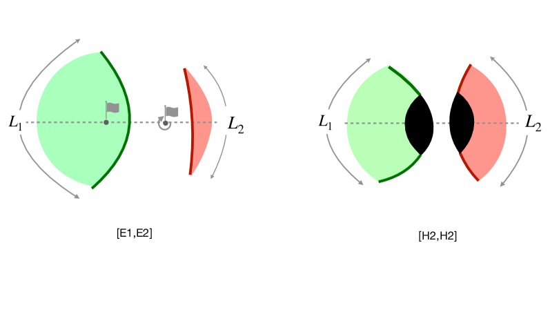
Figure 5: Schematic drawing of a low-temperature and a high-temperature solution, corresponding to pairs of type [E1,E2] and [H2,H2]. The broken line is the axis of reflection symmetry. The blueshift parameter $|\sigma|$ decreases monotonically until the string reaches either the turning point or the black-hole horizon.

Eqs. (4.11) imply that $2r_{j}r_{j}^{\prime}=1$. Inserting in eq. (4.2) gives

$$(x_{j}^{\prime})^{2}=r_{j}^{-2}\Bigl{(}g(\sigma)-{\ell_{j}^{2}\over 4\sigma r_{j}^{2}}\Bigr{)}\ .$$ (4.12)

Squaring now twice eq. (4.3) and replacing $(x_{j}^{\prime})^{2}$ from the above expressions leads to a quadratic equation for $g(\sigma)$, the ${\tiny\sigma\sigma}$ component of the worldsheet metric. This equation has a singular solution $g=0$, and a non-trivial one

$$g(\sigma)=\lambda^{2}\Biggl{[}\Bigl{(}\frac{2r_{1}r_{2}}{\ell_{1}\ell_{2}}\Bigr{)}^{2}\hskip-1.13809pt-\Bigl{(}\frac{r_{1}^{2}}{\ell_{1}^{\,2}}+\frac{r_{2}^{2}}{\ell_{2}^{\,2}}-\lambda^{2}\sigma\Bigr{)}^{2}\,\Biggr{]}^{-1}\hskip-5.406pt={\lambda^{2}\over A\sigma^{2}+2B\sigma+C}\,,$$ (4.13)

where in the second equality we used eqs. (4.11), and

$$A=(\lambda_{\rm max}^{2}-\lambda^{2})(\lambda^{2}-\lambda_{\rm min}^{2})\ ;$$

$$B=\lambda^{2}(M_{1}+M_{2})-\lambda_{0}^{2}(M_{1}-M_{2})\ ;\quad C=-(M_{1}-M_{2})^{2}\ .$$ (4.14)

We expressed the quadratic polynomial appearing in the denominator of (4.13) in terms of $M_{j},\lambda$ and the critical tensions, eqs. (4.8), in order to render manifest the fact that for $\lambda$ in the allowed range, $\lambda_{\rm min}<\lambda<\lambda_{\rm max}$, the coefficient $A$ is positive. This is required for $g(\sigma)$ to be positive near the boundary where $\sigma\to\infty$. In addition, $AC\leq 0$ which ensures that the two roots of the denominator in eq. (4.13)

$$\sigma_{\pm}={-B\pm(B^{2}-AC)^{1/2}\over A}$$ (4.15)

are real, and that the larger root $\sigma_{+}$ is non-negative. Inserting eq. (4.13) in eq. (4.12) and fixing the sign of the square root near the conformal boundary gives after a little algebra

$$\frac{x_{1}^{\prime}}{\ell_{1}}\,=\,-\frac{\sigma\,(\lambda^{2}+\lambda_{0}^{2})+M_{1}-M_{2}}{{2(\sigma+M_{1}\ell_{1}^{\,2})}\,\sqrt{A\sigma(\sigma-\sigma_{+})(\sigma-\sigma_{-})}}\ \ ,$$ (4.16a)

$$\frac{x_{2}^{\prime}}{\ell_{2}}\,=\,-\frac{\sigma\,(\lambda^{2}-\lambda_{0}^{2})+M_{2}-M_{1}}{{2(\sigma+M_{2}\ell_{2}^{\,2})}\,\sqrt{A\sigma(\sigma-\sigma_{+})(\sigma-\sigma_{-})}}\ \ .$$ (4.16b)

We may now confirm our earlier claim that if $\sigma_{+}>0$ then both $x_{1}^{\prime}\propto dx_{1}/dr_{1}$ and $x_{2}^{\prime}\propto dx_{2}/dr_{2}$ diverge at this point. Furthermore, since $\sigma+M_{j}\ell_{j}^{\,2}=r_{j}^{2}$ is positive, the $x_{j}^{\prime}$ are finite at all $\sigma>\sigma_{+}$. Thus $\sigma_{+}$ is the unique turning point of the string, as advertized.

Eqs. (4.11) and (4.16) give the general solution of the string equations for arbitrary mass parameters $M_{1},M_{2}$ of the green and pink slices. These must be determined by interior regularity, and by the Dirichlet conditions at the conformal boundary. Explicitly, the boundary conditions for the different slice types of figure 3 read:

$$L_{j}\ =\,2\int_{\,\sigma_{+}}^{\infty}d\sigma\,x_{j}^{\prime}\,\qquad\qquad{\text{for \ \ {\small E2, E2${}^{\prime}$}}}\ ;$$ (4.17a)

$$L_{j}\ =\ nP_{j}+\,2\int_{\,\sigma_{+}}^{\infty}d\sigma\,x_{j}^{\prime}\,\qquad{\text{ for \ \ {\small E1, H1}}}\ ;$$ (4.17b)

$$L_{j}\ =\ \Delta x_{j}\bigl{|}_{\rm Hor}\,+\,2\int_{\,\sigma_{+}}^{\infty}d\sigma\,x_{j}^{\prime}\,\qquad\quad{\text{ for \ \ {\small H2}}}\ .$$ (4.17c)

The integrals in these equations are the opening arcs, $\Delta x_{j}$, between the two endpoints of a half string. They can be expressed as complete elliptic integrals of the first, second and third kind, see appendix B. For the slices E1, H1 where $x_{j}$ is a periodic coordinate, we have denoted by $P_{j}>0$ its period, and by $n$ the string winding number. Finally for strings entering the horizon we denote by $\Delta x_{j}|_{\rm Hor}$ the opening arc between the two horizon-entry points in the $j$th coordinate chart.

Possible phases of the ICFT for given torus parameters $T,L_{j}$ must be solutions to one pair of conditions (4.17). Apart from interior regularity, we will also require that the string does not self-intersect. In principle, two string bits intersecting at an angle $\not=\pi$ could join into another string. Such string junctions would be the gravitational counterparts of interface fusion [65], and allowing them would make the holographic model much richer. To keep, however, our discussion simple we will only allow a single type of domain wall in this work.

The reader can easily convince herself that to avoid string intersections we must have $P_{j}>L_{j}$ and $n=1$ in (4.17b), and $\Delta x_{j}\bigl{|}_{\rm Hor}>0$ in (4.17c).

5 Phases: cold, hot $\&$ warm

Among the five slice types of figure 3, H2 stands apart because it can only pair with itself. This is because a horizon is a closed surface, so it cannot end on the domain wall. We will now show that the matching equations actually rule out several other pairs among the remaining slice types.

One pair that is easy to exclude is [H1,H1], i.e.  solutions that describe two black holes sitting on either side of the wall. Interior regularity would require in this case $M_{1}=M_{2}=(2\pi T)^{2}$. But eqs. (4.14) and (4.15) then imply that $\sigma_{+}=0$, so the wall cannot avoid the horizon leading to a contradiction.

This gives our first no-go lemma:

Note by contrast that superheavy domain walls ($\lambda>\lambda_{\rm max}$) inflate and could thus prevent the black holes from coalescing.

A second class of pairs one can exclude are the ‘centerless geometries’ [E2,E2], [E2,E2^′], [E2^′,E2] and [E2^′,E2^′]. We use the word ‘centerless’ for geometries that contain neither a center of global AdS, nor a black hole in its place (see fig. 3). If such solutions existed, all inertial observers would necessarily hit the domain wall since there would be neither a center where to rest, nor a horizon where to escape.

The argument excluding such solutions is based on a simple observation: What distinguishes the centerless slices E2 and E2^′ from those with a AdS center (E1) or a black hole (H1) is the sign of $x_{j}^{\prime}$ at the turning point,

$${\rm sign}\bigl{(}x_{j}^{\prime}\bigl{|}_{\sigma\approx\sigma_{+}}\bigr{)}\ =\begin{cases}+\quad{\rm for\ {\small E2},{\small E2}}^{\prime}\,,\\ -\quad{\rm for\ {\small E1},{\small H1}}\ .\end{cases}$$ (5.1)

Now from eqs. (4.16) one has

$$(\sigma+M_{1}\ell_{1}^{\,2})\,\frac{x_{1}^{\prime}}{\ell_{1}}+(\sigma+M_{2}\ell_{2}^{\,2})\,\frac{x_{2}^{\prime}}{\ell_{2}}\,<\,0\ ,$$ (5.2)

so both $x_{j}^{\prime}$ cannot be simultaneously positive. This holds for all $\sigma$, and hence also near the turning point QED. This is our second no-go lemma:

We can actually exploit this argument further. As is clear from eq. (4.16a), if $M_{1}>M_{2}$ then $x^{\prime}_{1}$ is manifestly negative, i.e. the green slice is of type E1 or H1. The pairs [E2^′,E1] and [E2^′,E2] for which the above inequality is automatic are thus ruled out. One can also show that $x^{\prime}_{2}|_{\sigma\approx\sigma_{+}}$ is negative if $M_{2}>0>M_{1}$. This is obvious from eq. (4.16b) in the range $\lambda>\lambda_{0}$, and less obvious but also true as can be checked by explicit calculation for $\lambda<\lambda_{0}$. The pairs [E1,E2^′] and [E2,E2^′] for which the above mass inequality is automatic, are thus also excluded.

Recall that the energy density of the $j$th CFT reads $\langle T_{tt}\rangle={1\over 2}\ell_{j}M_{j}$. Ruling out all pairs of E2^′ with E1 or E2 implies therefore that in the ground state the energy density must be everywhere negative. When one $L_{j}$ is much smaller than the other, the Casimir energy scales like $E_{0}\sim\#/L_{j}$. The fact that the coefficient $\#$ is negative means that the Casimir force is attractive, in agreement with general theorems [88, 89]. This is the third no-go lemma:

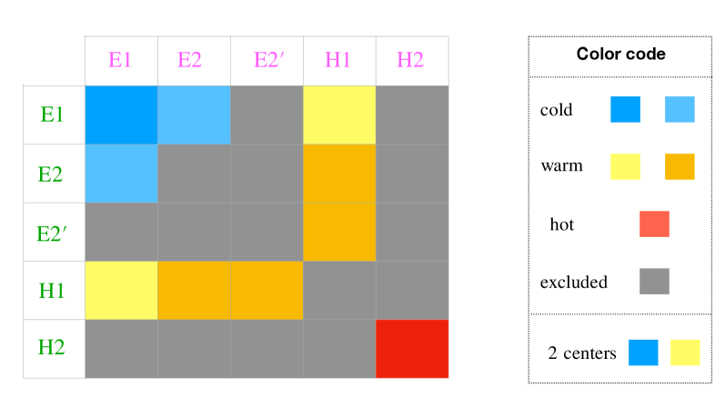
Figure 6: Phases of the domain-wall spacetime. The type of the green slice labels the rows of the table, and that of the pink slice the columns. In the hot (red) phase the wall enters the black-hole horizon, while in the warm (yellow) phases it avoids it. The cold (blue) phases have no black hole. Geometries in which an inertial observer is attracted to two different centers are indicated by a different shade (light yellow or darker blue).

We have collected for convenience all these conclusions in fig. 6. The table shows the eligible slice pairs, or the allowed topologies of static-domain-wall spacetimes. It also defines a color code for phase diagrams.

The light yellow phases that feature a wall between the black hole and an AdS restpoint are the gravitational avatars of the Faraday cage. Such solutions are easier to construct for larger $\lambda$. Domain walls lighter than $\lambda_{0}$, in particular, can never shield from a black hole in the ‘true-vacuum’ side. Indeed, as follows easily from eq. (4.16b), for $\lambda<\lambda_{0}$ and $M_{1}>0>M_{2}$, the sign of $x_{2}^{\prime}|_{\sigma\approx\sigma_{+}}$ is positive, so geometries of type [H1,E1] are excluded.

6 Equations of state

The different colors in figure 6 describe different phases of the system, since the corresponding geometries are topologically distinct. They differ in how the wall, the horizon (if one exists) and inertial observers intersect or avoid each other.

Let us now think thermodynamics. For fixed Lagrangian parameters $\lambda,\ell_{j}$, the canonical variables that determine the state of the system are the temperature $T$ and the volumes $L_{1},L_{2}$. Because of scale invariance only two dimensionless ratios matter:

$$\tau_{1}:=TL_{1}\ ,\quad\tau_{2}:=TL_{2}\qquad{\rm or}\quad\quad\gamma:={L_{1}\over L_{2}}={\tau_{1}\over\tau_{2}}\ .$$ (6.1)

The microcanonical variables, the energy density and the entropy of each subsystem, read (see section 2, and recall that $8\pi G=1$)

$${E_{j}\over L_{j}}={\ell_{j}\over 2}M_{j}\qquad{\rm and}\qquad S_{j}={r^{\rm H}_{j}\Delta x_{j}|_{\rm Hor}\over 4G}=2\pi\ell_{j}\sqrt{M_{j}}\,\Delta x_{j}|_{\rm Hor}\ .\ \$$ (6.2)

These are the natural parameters of the interior geometry. The entropies are scale invariant. The other key dimensionless variable is the mass ratio, viz. the ratio of energy densities per degree of freedom in the two CFTs

$$\mu:={M_{2}\over M_{1}}\ .$$ (6.3)

When several phases coexist the dominant one is the one with the lowest free energy $F=\sum_{j}(E_{j}-TS_{j})$. As a sanity check, we rederive $F$ from the renormalized on-shell gravitational action in appendix A.

The Dirichlet conditions, eqs. (4.17), give for each type of geometry two relations among the above variables that play the role of equations of state. They relate the natural interior parameters $S_{j}$ and $\mu$ to the variables $\tau_{j}$ and $\gamma$ of the boundary torus. Note that in each phase of the system since for horizonless slices $S_{j}=0$ and for slices with horizon $M_{j}=(2\pi T)^{2}$. In computing the phase diagram we will have to invert these equations of state.

6.1 High-$T$ phase

For fixed $L_{j}$ and very high temperature the black hole grows so large that it eats away a piece of the domain wall and the AdS rest points. The dominant solution is thus of type [H2,H2] and regularity fixes the mass parameters in both slices, $M_{1}=M_{2}=(2\pi T)^{2}$. The boundary conditions (4.17c) reduce in this case to simple equations for the opening horizon arcs $\Delta x_{j}|_{\rm Hor}$. Performing explicitly the integrals (see appendix B) gives

$$L_{1}-\Delta x_{1}\bigl{|}_{\rm Hor}\ =\ -{1\over\pi T}\,{\rm tanh}^{-1}\left({\ell_{1}(\lambda^{2}+\lambda^{2}_{0})\over 2\lambda}\right)\ ,$$ (6.4a)

$$L_{2}-\Delta x_{2}\bigl{|}_{\rm Hor}\ =\ -{1\over\pi T}\,{\rm tanh}^{-1}\left({\ell_{2}(\lambda^{2}-\lambda^{2}_{0})\over 2\lambda}\right)\ .$$ (6.4b)

For consistency we must have $\Delta x_{j}|_{\rm Hor}>0$, which is automatic if $\lambda>\lambda_{0}$. If $\lambda<\lambda_{0}$, on the other hand, positivity of $\Delta x_{2}|_{\rm Hor}$ puts a lower bound on $\tau_{2}$,

$$\tau_{2}\,\geq\,{1\over\pi}\,{\rm tanh}^{-1}\left({\ell_{2}(\lambda_{0}^{2}-\lambda^{2})\over 2\lambda}\right)\ :=\,\tau_{2}^{*}\ .$$ (6.5)

We see here a first interpretation of the critical tension $\lambda_{0}$ encountered in section 4.3. For walls lighter than $\lambda_{0}$ there is a region of parameter space where the hot solution ceases to exist, even as a metastable phase.

The total energy and entropy in the high-$T$ phase read

$$E_{\rm[hot]}\,=\,{1\over 2}(\ell_{1}L_{1}M_{1}+\ell_{2}L_{2}M_{2})\,=\,2\pi^{2}T^{2}\,(\ell_{1}L_{1}+\ell_{2}L_{2})\ ,$$ (6.6)

$$S_{\rm[hot]}=4\pi^{2}T\bigl{(}\ell_{1}\Delta x_{1}\bigl{|}_{\rm Hor}+\,\ell_{2}\Delta x_{2}\bigl{|}_{\rm Hor}\bigr{)}=4\pi^{2}T^{2}(\ell_{1}L_{1}+\ell_{2}L_{2})+2\log g_{I}\ ,\ \ \$$ (6.7)

where $\log g_{\rm I}\,$ is given by eq. (4.9) and the rightmost expression of the entropy follows from eqs. (6.4) and a straightforward reshuffling of the arctangent functions. This is a satisfying result. Indeed, the first term in the right-hand side of (6.7) is the thermal entropy of the two CFTs (being extensive these entropies cannot depend on the ratio $L_{1}/L_{2}$), while the second term is the entropy of the two interfaces on the circle. The Bekenstein-Hawking formula captures nicely both contributions.

Eqs.(6.4) and (6.7) show that shifting the $L_{j}$ at fixed $T$ does not change the entropy if and only if $\ell_{1}\,\delta L_{1}=-\ell_{2}\,\delta L_{2}$. Moving in particular a defect (for which $\ell_{1}=\ell_{2}$) without changing the volume $L_{1}+L_{2}$ is an adiabatic process, while moving a more general interface generates/absorbs entropy by modifying the density of degrees of freedom.

6.2 Low-$T$ phase(s)

Consider next the ground state of the system, at $T=0$. The dual geometry belongs to one of the three horizonless types: the double-center geometry [E1, E1], or the single-center ones [E1, E2] and [E2, E1] (see fig. 6). Here the entropies $S_{j}=0$, and the only relevant dimensionless variables are the volume and energy-density ratios, $\gamma$ and $\mu$. Note that they are both positive since $L_{j}>0$ and $M_{j}<0$ for both $j$.

The Dirichlet conditions (4.16) for horizonless geometries read

$$\sqrt{|M_{1}|}\,L_{1}=2\pi\,\delta_{{\mathbb{S}}_{1},{\rm E1}}-f_{1}(\mu)\ ,\qquad\sqrt{|M_{1}|}\,L_{2}={2\pi\over\sqrt{\mu}}\,\delta_{{\mathbb{S}}_{2},{\rm E1}}-f_{2}(\mu)\ ,$$ (6.8)

where $\delta_{{\mathbb{S}}_{j},{\rm E1}}=1$ if the $j$th slice is of type E1 and $\delta_{{\mathbb{S}}_{j},{\rm E1}}=0$ otherwise, and

$$f_{1}(\mu)\,=\,{\ell_{1}\over\sqrt{A}}\int_{s_{+}}^{\infty}ds{s(\lambda^{2}+\lambda_{0}^{2})-1+\mu\over(s-\ell_{1}^{\,2})\sqrt{s(s-s_{+})(s-s_{-})}}\ ,\ \ \$$ (6.9a)

$$f_{2}(\mu)\,=\,{\ell_{2}\over\sqrt{A}}\int_{s_{+}}^{\infty}ds{s(\lambda^{2}-\lambda_{0}^{2})+1-\mu\over(s-\mu\ell_{2}^{\,2})\sqrt{s(s-s_{+})(s-s_{-})}}\ ,\ \ \$$ (6.9b)

with

$$A\,s_{\pm}=\lambda^{2}(1+\mu)-\lambda_{0}^{2}(1-\mu)\pm 2\lambda\sqrt{{1-\mu\over\ell_{2}^{2}}+{\mu^{2}-\mu\over\ell_{1}^{2}}+\mu\lambda^{2}}\ \ .$$ (6.10)

The dummy integration variable $s$ is the appropriately rescaled blueshift factor of the string worldsheet, $s=\sigma/|M_{1}|$ .

Dividing the two sides of eqs. (6.8) gives $\gamma$ as a function of $\mu$ for each of the three possible topologies. If the ground state of the putative dual quantum-mechanical system was unique, we should find a single slice-pair type and value of $\mu$ for each value of $\gamma$. Numerical plots show that this is indeed the case. Specifically, we found that $\gamma(\mu)$ is a monotonically-increasing function of $\mu$ for any given slice pair, and that it changes continuously from one type of pair to another. We will return to these branch-changing ‘sweeping transitions’ in section 7. Let us stress that the uniqueness of the cold solution did not have to be automatic in classical gravity, nor in the dual large-$N$ quantum mechanics.

For most of the $(\ell_{j},\lambda)$ parameter space, as $\gamma$ ranges in $(0,\infty)$ the mass ratio $\mu$ covers also the entire range $(0,\infty)$. However, if $\ell_{1}<\ell_{2}$ (strict inequality) and for sufficiently light domain walls, we found that $\gamma$ vanishes at some positive $\mu=\mu_{0}(\lambda,\ell_{j})$. Below this critical value $\gamma$ becomes negative signaling that the wall self-intersects and the solution must be discarded. This leads to a striking phenomenon that we discuss in section 8.

6.3 Warm phases

The last set of solutions of the model are the yellow- or orange-coloured ones in fig. 6. Here the string avoids the horizon, so the slice pair is of type [H1,X] or [X,H1] with X one of the horizonless types: E1, E2 or E2^′.

Assume first that the black hole is on the green side of the wall, so that $M_{1}=(2\pi T)^{2}$. In terms of $\mu$ the Dirichlet conditions (4.17a, 4.17b) read:

$$2\pi T\Delta x_{1}\bigl{|}_{{\rm Hor}}-\,2\pi\tau_{1}=\tilde{f}_{1}(\mu)\ ,\qquad 2\pi\tau_{2}={2\pi\over\sqrt{-\mu}}\,\delta_{{\mathbb{S}}_{2},{\rm E1}}-\tilde{f}_{2}(\mu)\ ,$$ (6.11)

where

$$\tilde{f}_{1}(\mu)\,=\,{\ell_{1}\over\sqrt{A}}\int_{\tilde{s}_{+}}^{\infty}ds{s(\lambda^{2}+\lambda_{0}^{2})+1-\mu\over(s+\ell_{1}^{\,2})\sqrt{s(s-\tilde{s}_{+})(s-\tilde{s}_{-})}}\ ,\ \ \$$ (6.12a)

$$\tilde{f}_{2}(\mu)\,=\,{\ell_{2}\over\sqrt{A}}\int_{\tilde{s}_{+}}^{\infty}ds{s(\lambda^{2}-\lambda_{0}^{2})-1+\mu\over(s+\mu\ell_{2}^{\,2})\sqrt{s(s-\tilde{s}_{+})(s-\tilde{s}_{-})}}\ ,\ \ \$$ (6.12b)

and the roots $\tilde{s}_{\pm}=\sigma_{\pm}/M_{1}$ inside the square root are given by

$$A\,\tilde{s}_{\pm}=-\lambda^{2}(1+\mu)+\lambda_{0}^{2}(1-\mu)\pm 2\lambda\sqrt{{1-\mu\over\ell_{2}^{2}}+{\mu^{2}-\mu\over\ell_{1}^{2}}+\mu\lambda^{2}}\ \ .$$ (6.13)

In the first condition (6.11) we have used the fact that the period of the green slice that contains the horizon is $P_{1}=\Delta x_{1}|_{{\rm Hor}}$.

If the black hole is on the pink side of the wall, the conditions take a similar form in terms of the inverse mass ratio $\hat{\mu}=\mu^{-1}=M_{1}/M_{2}$,

$$2\pi T\Delta x_{2}\bigl{|}_{{\rm Hor}}-\,2\pi\tau_{2}={\hat{f}}_{2}(\hat{\mu})\ ,\quad 2\pi\tau_{1}={2\pi\over\sqrt{-\hat{\mu}}}\,\delta_{{\mathbb{S}}_{1},{\rm E1}}-\hat{f}_{1}(\hat{\mu})\ ,$$ (6.14)

where here

$$\hat{f}_{1}(\hat{\mu})\,=\,{\ell_{1}\over\sqrt{A}}\int_{\hat{s}_{+}}^{\infty}ds{s(\lambda^{2}+\lambda_{0}^{2})+\hat{\mu}-1\over(s+\hat{\mu}\ell_{1}^{\,2})\sqrt{s(s-\hat{s}_{+})(s-\hat{s}_{-})}}\ ,\ \ \$$ (6.15a)

$$\hat{f}_{2}(\mu)\,=\,{\ell_{2}\over\sqrt{A}}\int_{\hat{s}_{+}}^{\infty}ds{s(\lambda^{2}-\lambda_{0}^{2})-\hat{\mu}+1\over(s+\ell_{2}^{\,2})\sqrt{s(s-\hat{s}_{+})(s-\hat{s}_{-})}}\ .\ \ \$$ (6.15b)

and the roots $\hat{s}_{\pm}=\sigma_{\pm}/M_{2}$ inside the square root are given by

$$A\,\hat{s}_{\pm}=-\lambda^{2}(\hat{\mu}+1)+\lambda_{0}^{2}(\hat{\mu}-1)\pm 2\lambda\sqrt{{\hat{\mu}^{2}-\hat{\mu}\over\ell_{2}^{2}}+{1-\hat{\mu}\over\ell_{1}^{2}}+\hat{\mu}\lambda^{2}}\ \ .$$ (6.16)

The functions $\tilde{f}_{j}$ and $\hat{f}_{j}$, as well as the $f_{j}$ of the cold phase, derive from the same basic formulae (4.16a, 4.16b) and differ only by a few signs. We chose to write them out separately because these signs are important. Note also that while in cold solutions $\mu$ is always positive, here $\mu$ and its inverse $\hat{\mu}$ can have either sign.

All the values of  $\mu$  and  $\hat{\mu}$  do not, however, correspond to admissible solutions. For a pair of type [H1,X] we must demand (i) that the right-hand sides in (6.11) be positive – the non-intersection requirement, and (ii) that $x_{1}^{\prime}|_{\sigma\approx\sigma_{+}}$ be negative – the turning point condition (5.1). Likewise for solutions of type [X, H1] we must demand that the right-hand sides in (6.14) be positive and that $x_{2}^{\prime}|_{\sigma\approx\sigma_{+}}$ be negative.

The turning-point requirement is easy to implement. In the [H1,X] case, $x_{1}^{\prime}|_{\sigma\approx\sigma_{+}}$ is negative when the numerator of the integrand in (6.12a), evaluated at at $s=\tilde{s}_{+}$, is positive. Likewise for the [X,H1] pairs, $\,x_{2}^{\prime}|_{\sigma\approx\sigma_{+}}$ is negative when the numerator of the integrand in (6.15b), evaluated at at $s=\hat{s}_{+}$, is positive. After a little algebra these conditions take a simple form

$${\rm for}\ \ {\rm[H1,X]}\quad\mu\in(-\infty,1]\ ;\qquad{\rm for}\ \ {\rm[X,H1]}\quad\hat{\mu}=\mu^{-1}\in(-\infty,1]\ .\ \ \$$ (6.17)

Recalling that $\mu=\hat{\mu}^{-1}=M_{2}/M_{1}$, we conclude that in all the cases the energy density per degree of freedom in the horizonless slice is lower than the corresponding density in the black hole slice.

This agrees with physical intuition: the energy density per degree of freedom in the cooler CFT is less than the thermal density $\pi T^{2}/6$ – the interfaces did not let the theory thermalize. When $\mu\to 1$ or $\hat{\mu}\to 1$, the wall enters the horizon and the energy is equipartitioned.

This completes our discussion of the equations of state. To summarize, these equations relate the parameters of the interior geometry ($\mu,S_{j}$) to those of the conformal boundary ($\gamma,\tau_{j}$). The relation involves elementary functions in the hot phase, and was reduced to a single function $\gamma(\mu)$, that can be readily plotted, in the cold phases. Furthermore at any given point in parameter space the hot and cold solutions, when they exist, are unique. The excluded regions are $\tau_{2}<\tau_{2}^{*}(\lambda,\ell_{j})$ for the hot solutions, and $\mu>\mu_{0}(\lambda,\ell_{j})$ for the cold solution with $\mu_{0}$ the point where $\gamma=0$.

In warm phases the story is richer since more than one solutions typically coexist at any given value of $(\gamma,\tau_{j})$. Some solutions have negative specific heat, as we will discuss later. To find the parameter regions where different solutions exist requires inverting the relation between ($\gamma,\tau_{j}$) and ($\mu,S_{j}$). We will do this analytically in some limiting cases, and numerically to compute the full phase diagram in section 9.

7 Phase transitions

The transitions between different phases are of three kinds:

• Hawking-Page transitions describing the formation of a black hole. These transitions from the cold to the hot or warm phases of fig. 6 are always first order;

• Warm-to-hot transitions during which part of the wall is captured by the horizon. We will show that these transitions are also first-order;

• Sweeping transitions where the wall sweeps away a center of global AdS, i.e.  a rest point for inertial observers. These are continuous transitions between the one- and two-center phases of fig. 6.

It is instructive to picture these transitions by plotting the metric factor $g_{tt}$ while traversing space along the axis of reflection symmetry. The curve changes qualitatively as shown in figure 9, illustrating the topological nature of the transitions on the gravity side.

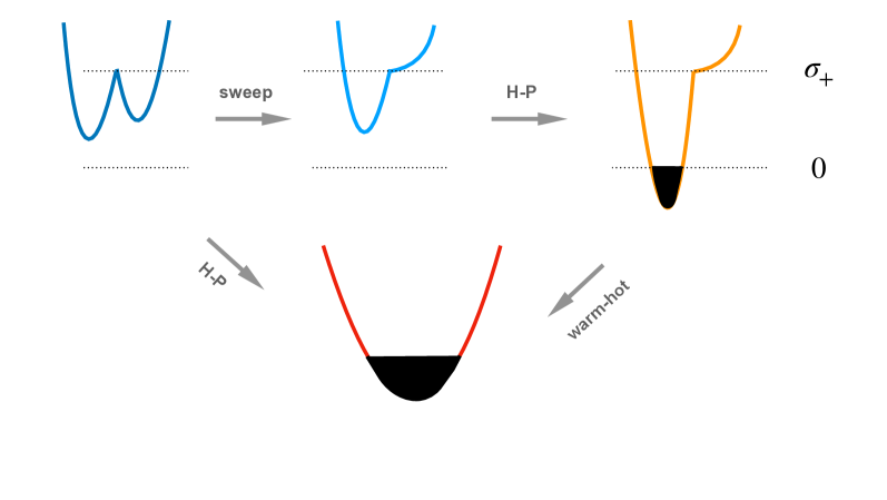
Figure 7: Curves of the blueshift factor $g_{tt}$ as one traverses space along the $Z_{2}$ symmetry axis. The color code is the same as in fig. 6. The wall is located at the turning point $g_{tt}=\sigma_{+}$ where the curve is discontinuous. The grey arrows indicate possible transitions. The blackened parts of the curves are regions behind the horizon.

Before embarking in numerical plots, we will first do the following things: (i) Comment on the ICFT interpretation of these transitions; (ii) Compute the sweeping transitions analytically; and (iii) Prove that the warm-to-hot transitions are first order, i.e. that one cannot lower the wall to the horizon continuously by varying the boundary data.

7.1 ICFT interpretation

When a holographic dual exists, Witten has argued that the appearance of a black hole at the Hawking-Page (HP) transition signals deconfinement in the gauge theory [90]. Assuming this interpretation  leads to the conclusion that in warm phases a confined theory coexists with a deconfined one. We will see below that such coexistence is easier when the confined theory is CFT₂, i.e. the theory with the larger central charge. This is natural from the gravitational perspective. Solutions of type [H1, X] are more likely than solutions of type [X, H1] because a black hole forms more readily on the ‘true-vacuum’ side of the wall. We will actually provide some evidence later that if $c_{2}>3c_{1}$ there are no equilibrium phases at all in which CFT₂ is deconfined while CFT₁ stays confined.

The question that jumps to one’s mind is what happens for thick walls, where one expects a warm-to-hot crossover rather than a sharp transition. One possibility is that the coexistence of confined and deconfined phases is impossible in microscopic holographic models. Alternatively, an appropriately defined Polyakov loop [90] could provide a sharp order parameter for this transition.

For sweeping transitions the puzzle is the other way around. Here a sharp order parameter exists in classical gravity – it is the number of rest points for inertial observers. This can be defined both for thin- and for thick-wall geometriess. The interpretation on the field theory side is however unclear. The transitions could be related to properties of the low-lying spectrum at infinite $N$, or to the entanglement structure of the ground state.

We leave these questions open for future work.

7.2 Sweeping transitions

Sweeping transitions are continuous transitions that happen at fixed values of the mass ratio $\mu$. We will prove these statements here.

Assume for now continuity, and let the $j$th slice go from type E1 to type E2. The transition occurs when the string turning point and the center of the $j$th AdS slice coincide, i.e. when

$$r_{j}(\sigma_{+})=\sqrt{\sigma_{+}+M_{j}\ell_{j}^{2}}\,=\,0\ .$$ (7.1)

Clearly this has a solution only if $M_{j}<0$. Inserting in (7.1) the expressions (4.15) - (4.14) for $\sigma_{+}$ gives two equations for the critical values of $\mu$ with the following solutions

$$\mu_{1}^{*}={1-\ell_{2}^{\,2}\lambda^{2}\over\ell_{2}^{2}/\ell_{1}^{2}}\quad\ {\rm and}\quad\ \mu_{2}^{*}={\ell_{1}^{2}/\ell_{2}^{2}\over 1-\ell_{1}^{\,2}\lambda^{2}}\ \ .$$ (7.2)

In the low-$T$ phases both $M_{j}$ are negative and $\mu$ is positive. Furthermore, a little algebra shows that for all $\lambda\in(\lambda_{\rm min},\,\lambda_{\rm max})$  the following is true

$$x_{1}^{\prime}\bigl{|}_{\sigma\approx\sigma_{+}}<0\quad{\rm at}\ \ \mu\gg 1\ \quad{\rm and}\quad x_{2}^{\prime}\bigl{|}_{\sigma\approx\sigma_{+}}<0\quad{\rm at}\ \ \mu\ll 1\,.\ \$$ (7.3)

This means that for $\mu\gg 1$ the green slice is of type E1, and for $\mu\ll 1$ the pink slice is of type E1. A sweeping transition can occur if the critical mass ratios (7.2) are in the allowed range. We distinguish three regimes of $\lambda$:

• Heavy ($\lambda>1/\ell_{1}$): None of the $\mu_{j}^{*}\,$ is positive, so the solution is of type [E1,E1] for all $\mu$, i.e. cold solutions are always double-center ;

• Intermediate (${1/\ell_{1}}>\lambda>1/\ell_{2}$): Only $\mu_{2}^{*}\,$ is positive. If this is inside the range of non-intersecting walls, the solution goes from [E1,E2] at large $\mu\,$, to [E1,E1] at small $\mu$. Otherwise the geometry is always of the single-center type [E1,E2] ;

• Light ($\lambda<1/\ell_{2}$): Both $\mu_{1}^{*}\,$ and $\mu_{2}^{*}\,$ are positive, so there is the possibility of two sweeping transitions: from [E2,E1] at small $\mu$ to [E1,E2] at large $\mu$ passing through the double-center type [E1,E1] . Note that since $\lambda_{\rm min}=1/\ell_{1}-1/\ell_{2}$, this range of $\lambda$ only exists if $\ell_{2}<2\ell_{1}$, i.e.  when CFT₂ has no more than twice the number of degrees of freedom of the more depleted CFT₁.

We can now confirm that sweeping transitions are continuous, not only in terms of the mass ratio $\mu$ but also in terms of the ratio of volumes $\gamma$. To this end we expand the relations (6.8) around the above critical points and show that the $L_{j}$ vary indeed continuously across the transition. The calculations can be found in appendix  C .

For the warm phases we proceed along similar lines. One of the two $M_{j}$ is now equal to $(2\pi T)^{2}>0$, so sweeping transitions may only occur for negative $\mu$. Consider first warm solutions of type [H1,X] with the black hole in the ‘true vacuum’ side. A little calculation shows that $\,x_{2}^{\prime}|_{\sigma\approx\sigma_{+}}$ is negative, i.e. X=E1,  if and only if

$$\lambda>{1\over\ell_{1}}\qquad{\rm and}\qquad\mu<\mu_{2}^{*}<0\ .$$ (7.4)

Recall that when X=E1 some inertial observers can be shielded from the black hole by taking refuge at the restpoint of the pink slice. We see that this is only possible for heavy walls ($\lambda>1/\ell_{1}$) and for $\mu<\mu_{2}^{*}$. A sweeping transition [H1,E1] $\to$ [H1,E2] takes place at $\mu=\mu_{2}^{*}$.

Consider finally a black hole in the ‘false vacuum’ side, namely warm solutions of type [X,H1]. Here $\,x_{1}^{\prime}|_{\sigma\approx\sigma_{+}}$ is negative, i.e. $X$ has a rest point, if and only if the following conditions are satisfied

$$\lambda>{1\over\ell_{2}}\qquad{\rm and}\qquad\hat{\mu}:=\mu^{-1}<(\mu_{1}^{*})^{-1}<0\ .$$ (7.5)

Shielding from the black hole looks here easier, both heavy and intermediate-tension walls can do it. In reality, however, we have found that solutions with the black hole in the ‘false vacuum’ side are rare, and that the above inequality pushes $\hat{\mu}$ outside the admissible range.

The general trend emerging from the analysis is that the heavier the wall the more likely are the two-center geometries. A suggestive calculation actually shows that

$${\partial\sigma_{+}\over\partial\lambda}\Bigl{|}_{M_{j}\ {\rm fixed}}\ \ {\rm is}\ \begin{cases}{\textrm{ positive\ \ for \ two-center\ solutions}}\\ \,{\textrm{negative\ \ for \ single-center\ solutions}}\end{cases}$$ (7.6)

where the word ‘center’ here includes both an AdS restpoint and a black hole. At fixed energy densities a single center is therefore pulled closer to a heavier wall, while two centers are instead pushed away. It might be interesting to also compute ${\partial\sigma_{+}/\partial\lambda}$ and ${\partial V/\partial\lambda}$ at $L_{j}$ fixed, where $V$ is the regularized volume of the interior space. In the special case of the vacuum solution with an AdS₂ wall, the volume (and the associated complexity [100]) can be seen to grow with the tension $\lambda$.

7.3 Warm-to-hot transitions

In warm-to-hot transitions the thin domain wall enters the black-hole horizon. One may have expected this to happen continuously, i.e. to be able to lower the wall to the horizon smoothly, by slowly varying the boundary data $L_{j},T$. We will now show that, if the tension $\lambda$ is fixed, the transition is actually always first order.

Note first that in warm solutions the slice that contains the black hole has $M_{j}=(2\pi T)^{2}$. If the string turning point approaches continuously the horizon, then $\sigma_{+}\to 0$. From eqs. (4.14, 4.15) we see that this can happen if and only if $(M_{1}-M_{2})\to 0$, which implies in passing that the solution must necessarily be of type [H1,E2^′] or [E2^′,H1]. Expanding around this putative point where the wall touches the horizon we set

$${M_{1}-M_{2}\over M_{1}+M_{2}}:=\delta\quad{\rm with}\quad|\delta|\ll 1\ \ \Longrightarrow\ \ \sigma_{+}\approx\biggl{(}{2\pi T\over\lambda}\biggr{)}^{2}\delta^{2}\,.$$ (7.7)

Recalling that the horizonless slice has the smaller $M_{j}$ we see that for positive $\delta$ the black hole must be in the green slice and $\mu=1-2\delta+{\cal O}(\delta^{2})$, while for negative $\delta$ the black hole is in the pink slice and $\hat{\mu}=1+2\delta+{\cal O}(\delta^{2})$.

The second option can be immediately ruled out since it is impossible to satisfy the boundary conditions (6.14). Indeed, $\hat{f}_{1}(\hat{\mu}\approx 1)$ is manifetsly positive, as is clear from eq. (6.15a), and we have assumed that $\mathbb{S}_{1}$ is of type E2^′. Thus the second condition (6.14) cannot be obeyed. By the same reasonning we see that for $\delta$ positive, and since now $\mathbb{S}_{2}$ is of type E2^′, we need that $\tilde{f}_{2}(\mu\approx 1)$ be negative. As is clear from the expression (6.12b) this implies that $\lambda<\lambda_{0}$.

The upshot of the discussion is that a warm solution arbitrarily close to the hot solution may exist only if $\lambda<\lambda_{0}$ and if the black hole is on the true-vacuum side.

It is easy to see that under these conditions the two branches of solution indeed meet at $\mu=1$, $\Delta x_{2}|_{{\rm Hor}}=0$ and hence from (6.4b)

$$\tau_{2}\,=\,{1\over\pi}\,{\rm tanh}^{-1}\left({\ell_{2}(\lambda_{0}^{2}-\lambda^{2})\over 2\lambda}\right)\,:=\,\tau_{2}^{*}\,.$$ (7.8)

Recall from section 6.1 that this is the limiting value for the existence of the hot solution – the solution ceases to exist at $\tau_{2}<\tau_{2}^{*}\,.$ The nearby warm solution could in principle take over in this forbidden range, provided that $\tau_{2}(\delta)$ decreases as $\delta$ moves away from zero. It actually turns out that $\tau_{2}(\delta)$ initially increases for small $\delta$, so this last possibility for a continuous warm-to-hot transition is also ruled out.

To see why this is so, expand (6.11) and (6.12b) around $\mu=1$,

$$\tilde{s}_{+}={\delta^{2}\over\lambda^{2}}+{\cal O}(\delta^{3})\,,\quad\tilde{s}_{-}=-{4\lambda^{2}\over A}\Bigl{(}1-\delta(1+{\lambda_{0}^{2}\over\lambda^{2}})\Bigr{)}+{\cal O}(\delta^{2})\,,\quad$$

and shift the integration variable $s:=y+\tilde{s}_{+}$ so that (6.12b) reads

$$2\pi\,\tau_{2}(\delta)={\ell_{2}\over\sqrt{A}}\int_{0}^{\infty}dy\left[{y(\lambda_{0}^{2}-\lambda^{2})+2\delta\over(y+\mu\ell_{2}^{2})\sqrt{y(y+\tilde{s}_{+})(y-\tilde{s}_{-})}}+{\cal O}(\delta^{2})\right]\ .$$ (7.9)

We neglected in the integrand all contributions of ${\cal O}(\delta^{2})$ except for the $\tilde{s}_{+}$ in the denominator that regulates the logarithmic divergence of the ${\cal O}(\delta\log\delta)$ correction. Now use the inequalities

$${y(\lambda_{0}^{2}-\lambda^{2})+2\delta\over\sqrt{(y+\tilde{s}_{+})(y-\tilde{s}_{-})}}>{y(\lambda_{0}^{2}-\lambda^{2})+2\delta\over\sqrt{(y+\delta^{2}/\lambda^{2})(y+4\lambda^{2}/A)}}>{\sqrt{y}(\lambda_{0}^{2}-\lambda^{2})\over\sqrt{(y+4\lambda^{2}/A)}}\ ,$$

where the second one is equivalent to $2\delta>(\lambda_{0}^{2}/\lambda^{2}-1)\delta^{2}$, which is true for small enough $\delta$. Plugging in (7.9) shows that $\tau_{2}(\delta)>\tau_{2}(0)$ at the leading order in $\delta$, proving our claim.

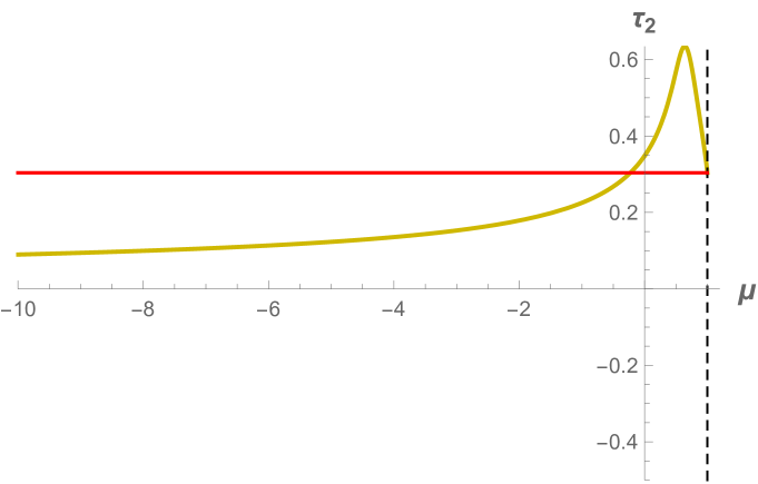
Figure 8: The function $\tau_{2}(\mu)$ in the [H1,E2] and [H1,E2^′] branches of solutions, for $2\ell_{2}=3\ell_{1}$ and $\lambda={3/5\ell_{2}}<\lambda_{0}={\sqrt{5}/2\ell_{2}}$ . The red line indicates the bound $\tau_{2}^{*}$ below which the hot solution ceases to exist.

A typical $\tau_{2}(\mu)$   in the [H1,E2] and [H1,E2^′] branch of solutions, and for $\lambda<\lambda_{0}$, is plotted in figure 8. The function grows initially as $\mu$ moves away from 1, reaches a maximum value and then turns around and goes to zero as $\mu\to-\infty$. The red line indicates the limiting value $\tau_{2}^{*}$ below which there is no hot solution. For $\tau_{2}$ slightly above $\tau_{2}^{*}$ we see that there are three coexisting black holes, the hot and two warm ones. For $\tau_{2}<\tau_{2}^{*}$, on the other hand, only one warm solution survives, but it describes a wall at a finite distance from the horizon. Whether this is the dominant solution or not, the transition is therefore necessarily first order.

8 Exotic fusion and bubbles

Before proceeding to the phase diagram, we pause here to discuss the peculiar phenomenon announced earlier, in section 6.2. This arises in the limits $\gamma=L_{1}/L_{2}\to 0$ or $\gamma\to\infty$, with $L_{1}+L_{2}$ and $T$ kept fixed. In these limits the conformal boundary of one slice shrinks to a point.

Consider for definiteness the limit $L_{1}\to 0$. In the language of the dual field theory the interface and anti-interface fuse in this limit into a defect of CFT₂. The naive expectation, based on free-field calculations [65, 101, 102], is that this is the trivial (or identity) defect. Accordingly, the green interior slice should recede to the conformal boundary, leaving as the only remnant a (divergent) Casimir energy.

We have found that this expectation is not always borne out as we will now explain.

Suppose first that the surviving CFT₂ is in its ground state, and that the result of the interface-antiinterface fusion is the expected trivial defect. The geometry should in this case approach global AdS₃ of radius $\ell_{2}$, with $M_{2}$ tending to $-(2\pi/L_{2})^{2}$, see section 2. Furthermore, $\sigma_{+}$ should go to infinity in order for the green slice to shrink towards the ultraviolet region. As seen from eqs. (4.15, 4.14) this requires $M_{1}\to-\infty$, so that $\mu\,$ should vanish together with $\gamma$. This is indeed what happens in much of the $(\lambda,\ell_{1},\ell_{2})$ parameter space. One finds $\mu\sim\gamma^{2}\to 0$, a scaling compatible with the expected Casimir energy $\sim\#/L_{1}$.

Nevertheless, sometimes $\gamma$ vanishes at finite $\mu_{0}$. In such cases, as $\mu\to\mu_{0}$ the green slice does not disappear even though its conformal boundary has shrunk to a point. This is illustrated by the left figure 9, which shows a static bubble of ‘true vacuum’ suspended from a point on the boundary of the ‘false vacuum’. To convince ourselves that the phenomenon is real, we give an analytic proof in appendix D of the existence of such suspended bubbles in at least one region of parameters ($\ell_{2}>\ell_{1}$ and $\lambda\approx\lambda_{\rm min}>0$). Furthermore, since the vacuum solution for a given $\gamma$ is unique, there is no other competing solution. In the example of appendix D, in particular, $\gamma$ is finite and negative at $\mu=0$.

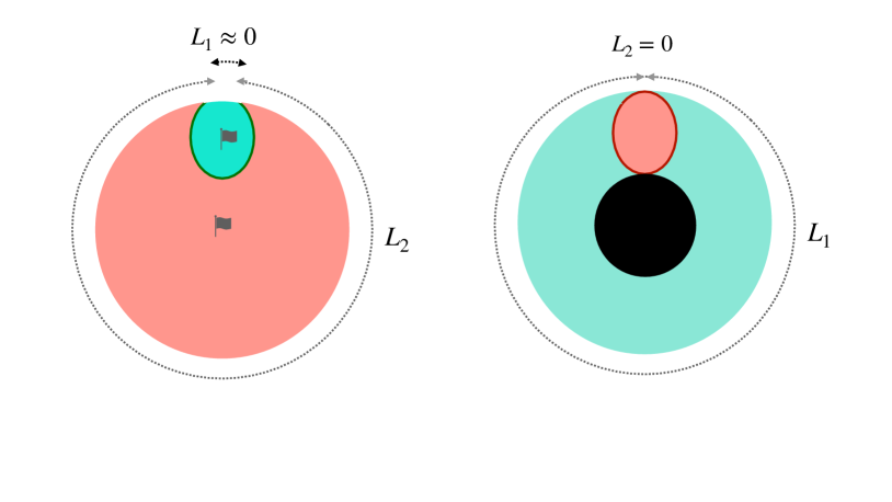
Figure 9: Left: A bubble of true vacuum that survives inside the false vacuum despite the fact that its conformal boundary shrinks to a point. Right: A bubble of false vacuum with $\lambda=\lambda_{0}$ inscribed between the boundary and the horizon of a black hole.

In the language of field theory this is a striking phenomenon. It implies that interface and anti-interface do not annihilate, but fuse into an exotic defect generating spontaneously a new scale in the process. This is the blueshift at the tip of the bubble, $\sigma_{+}(\mu_{0},L_{2})$, or better the corresponding frequency scale $r_{2}(\sigma_{+})$ in the D(efect)CFT.

The phenomenon is not symmetric under the exchange $1\leftrightarrow 2$. Static bubbles of the false vacuum (pink) spacetime inside the true (green) vacuum do not seem to exist. We proved this analytically for $\lambda<\lambda_{0}$, and numerically for all other values of the tension. We have also found that the suspended green bubble can be of type E1, i.e. have a center. The redshift factor $g_{tt}$ inside the bubble can even be lower than in the surrounding space, so that the bubble hosts the excitations of lowest energy. We did not show this analytically, but the numerical evidence is compeling.

Do suspended bubbles also exist when the surrounding spacetime contains a black hole ? The answer is affirmative as one can show semi-analytically by focussing on the region $\lambda\approx\lambda_{0}$. We have seen in the previous section that near this critical tension there exist warm solutions of type [H1,E2^′] with the wall arbitrarily close the horizon. Let us consider the function $\tau_{2}(\mu,\lambda)$ given in this branch of solutions by eqs. (6.12b) and (6.11) (with $\mathbb{S}_{2}\not=$E1). This is a continuous function in both arguments, so as $\lambda$ increases past $\lambda_{0}$, $\tau_{2}(1)$ goes from positive to negative with the overall shape of the function varying smoothly. This is illustrated in figure 10, where we plot $\tau_{2}(\mu)$ for $\lambda$ slightly below and slightly above $\lambda_{0}$. It should be clear from these plots that for $\lambda>\lambda_{0}$ (the plot on the right) $\tau_{2}$ vanishes at a finite $\mu\approx 1$. This is a warm bubble solution, as advertized.

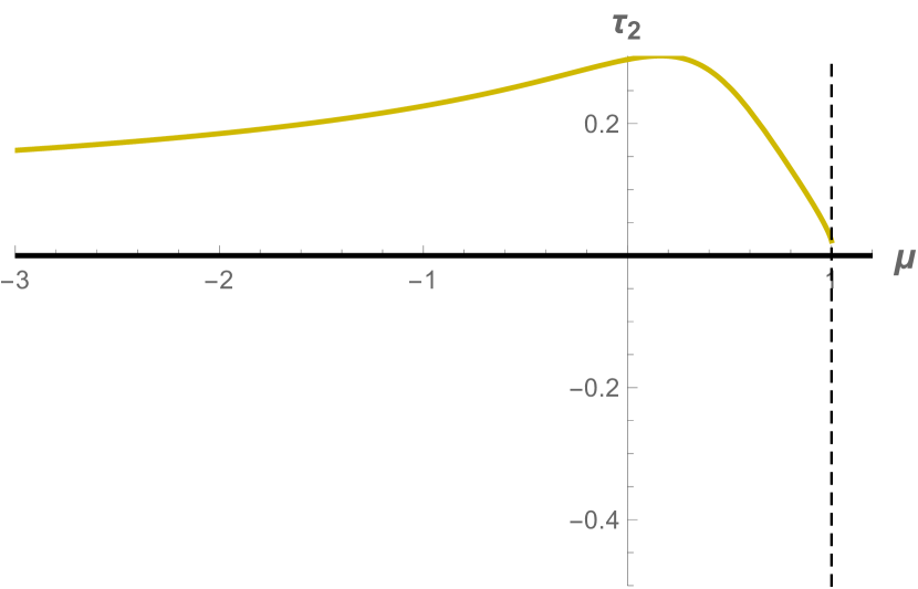
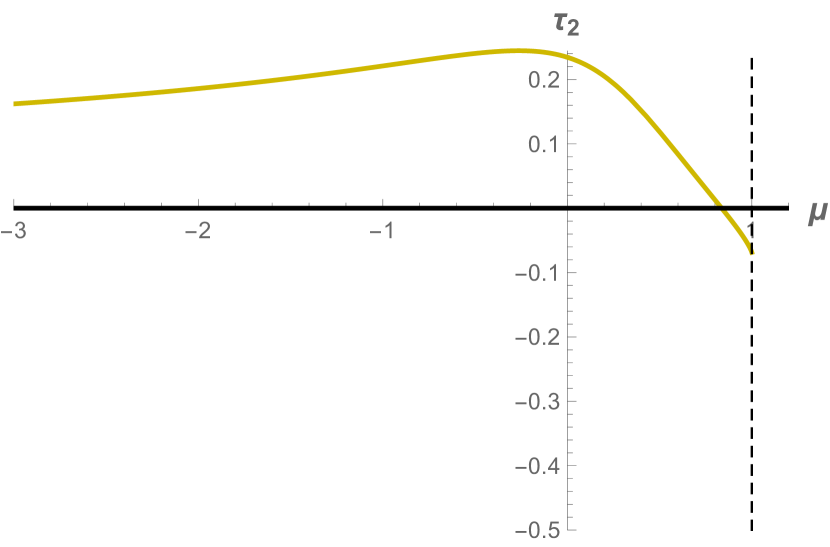
Figure 10: Plots of the function $\tau_{2}(\mu)$ in the [H1,E2] or [H1,E2^′] branch of solutions for $\ell_{2}/\ell_{1}=1.5$. The critical tension is $\lambda_{0}\ell_{2}\approx 1.12$. The curve on the left is for $\lambda_{0}\ell_{2}=1.05$, and the curve on the right for $\lambda_{0}\ell_{2}=1.35$.

We have found more generally that warm bubbles can be also of type E1, thus acting as a suspended Faraday cage that protects inertial observers from falling towards the horizon of the black hole. Contrary, however, to what happened for the ground state, warm bubble solutions are not unique. There is always a competing solution at $\mu\to-\infty$, and it is the dominant one by virtue of its divergent negative Casimir energy. A stability analysis would show if warm bubble solutions can be metastable and long-lived, but this is beyond our present scope.

As for warm bubbles of type [X, H1], that is with the black hole in the false-vacuum slice, these also exist but only if $\ell_{2}<3\ell_{1}$. Indeed, as we will see in a moment, when $\ell_{2}>3\ell_{1}$ the wall cannot avoid a horizon located on the false-vacuum side.

Finally simple inspection of fig. 10 shows that by varying the tension, the bubble solutions for $\lambda>\lambda_{0}$ go over smoothly to the hot solution at $\lambda=\lambda_{0}$. At this critical tension the bubble is inscribed between the horizon and the conformal boundary, as in figure 9. This gives another meaning to $\lambda_{0}$: Only walls with this tension may touch the horizon without falling inside.

9 Phase diagrams

In this last section of the paper we present numerical plots of the phase diagram of the model. We work in the canonical ensemble, so the variables are the temperature and volumes, or by scale invariance two of the dimensionless ratios defined in (6.1). We choose these to be $\,\tau=\tau_{1}+\tau_{2}=T(L_{1}+L_{2})$ and $\,\gamma=L_{1}/L_{2}$. The color code is as in fig. 6.

We plot the phase diagram for different values of the action parameters $\ell_{1},\ell_{2},\lambda$. Since our analysis is classical in gravity, Newton’s constant $G$ plays no role. Only two dimensionless ratios matter, for instance

$$b:={\ell_{2}\over\ell_{1}}={c_{2}\over c_{1}}\geq 1\qquad{\rm and}\quad\kappa:=\lambda\ell_{2}\in(b-1,b+1)\ .$$ (9.1)

The value $b=1$ corresponds to a defect CFT, while $b\gg 1$ is the opposite “near void” limit in which the degrees of freedom of CFT₂ ovewhelm those of CFT₁. The true vacuum approaches in this limit the infinite-radius AdS, and/or the false vacuum approaches flat spacetime. The critical tension $\lambda_{0}$ corresponds to $\kappa_{0}=\sqrt{b^{2}-1}$.

To plot the phase diagrams we solved numerically for $\mu$ in terms of the boundary data $(\gamma,\tau)$ and for all types of slice pair, and compared their free energies when solutions of different type coexist. As explained in the introduction, although the interpretation is different, our diagrams are related to the ones of Simidzija and Van Raamsdonk [29] by double-Wick rotation (special to 2+1 dimensions). Since time in this reference is non-compact, only the boundaries of our phase diagrams, at $\gamma=0$ or $\gamma=\infty$, can be compared. The roles of thermal AdS and BTZ are also exchanged

9.1 Defect CFT

Consider first $b=1$. By symmetry, we may restrict in this case to $\gamma\geq 1$. Figure  11 presents the phase diagram in the $(\gamma,\tau)$ plane for a very light ($\kappa=0.03$) and a very heavy ($\kappa=1.8$) domain wall. For the light, nearly tensionless, wall the phase diagram approaches that of a homogeneous CFT. The low-$T$ solution is single-center, and the Hawking-Page (HP) transition occurs at $\tau\approx 1$. Light domain walls follow closely geodesic curves, and avoid the horizon in a large region of parameter space. 

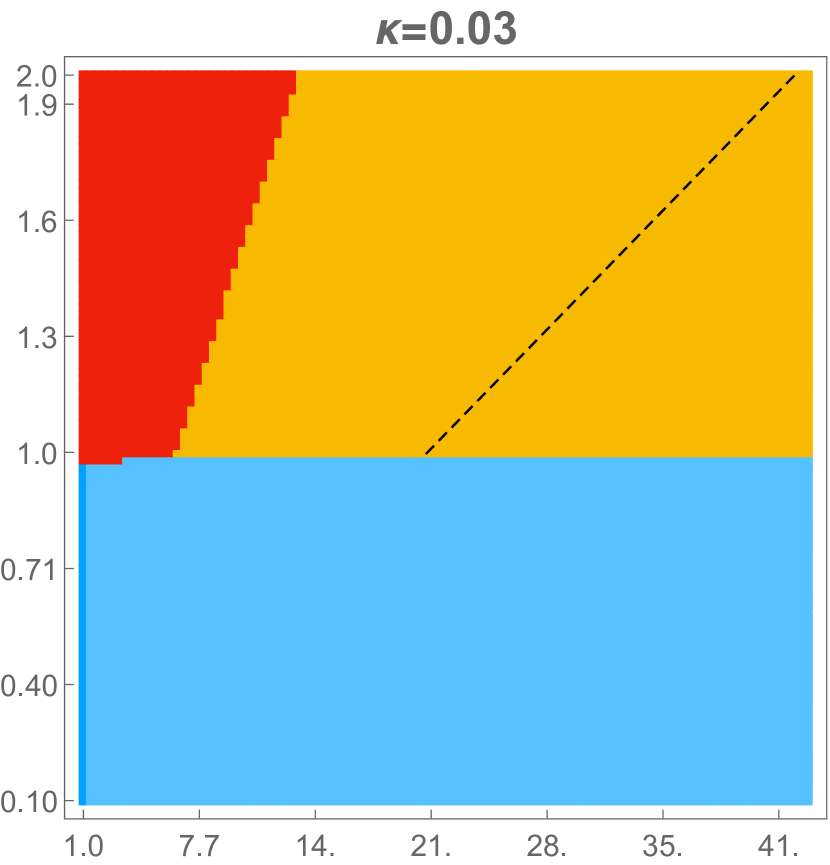
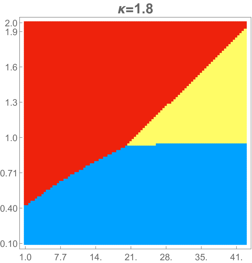
Figure 11: Phase diagrams of a very light (left) and a very heavy (right) domain wall between degenerate vacua ($b=1$). The horizontal and vertical axes are $\gamma$ and $\tau$. The broken line in the left diagram separates solutions of type [H1, E2^′] and [H1,E2] that only differ in the sign of the energy of the horizonless slice. The color code is as in fig. 6.

Comparing the left with the right figure 11 shows that heavy walls facilitate the formation of the black hole and have a harder time staying outside. Indeed, in the right figure the HP transition occurs at lower $T$, and the warm phase recedes to $L_{1}\gg L_{2}$. Furthermore, both the cold and the warm solutions have now an additional AdS restpoint. This confirms the intuition that heavier walls repel probe masses more strongly, and can shield them from falling inside the black hole.

The transition that sweeps away this AdS restpoint is shown explicitly in the phase diagrams of figure 12. Recall from the analysis of section 7.2 that in the low-$T$ phase such transitions happen for $\lambda<1/\ell_{1}\Longrightarrow\kappa<b=1$. Furthermore, the transitions take place at the critical mass ratios $\mu_{j}^{*}\,$, given by eq. (7.2). Since in cold solutions the relation between $\mu$ and $\gamma$ is one-to-one, the dark-light blue critical lines are lines of constant $\gamma$. These statements are in perfect agreement with the findings of fig. 12.

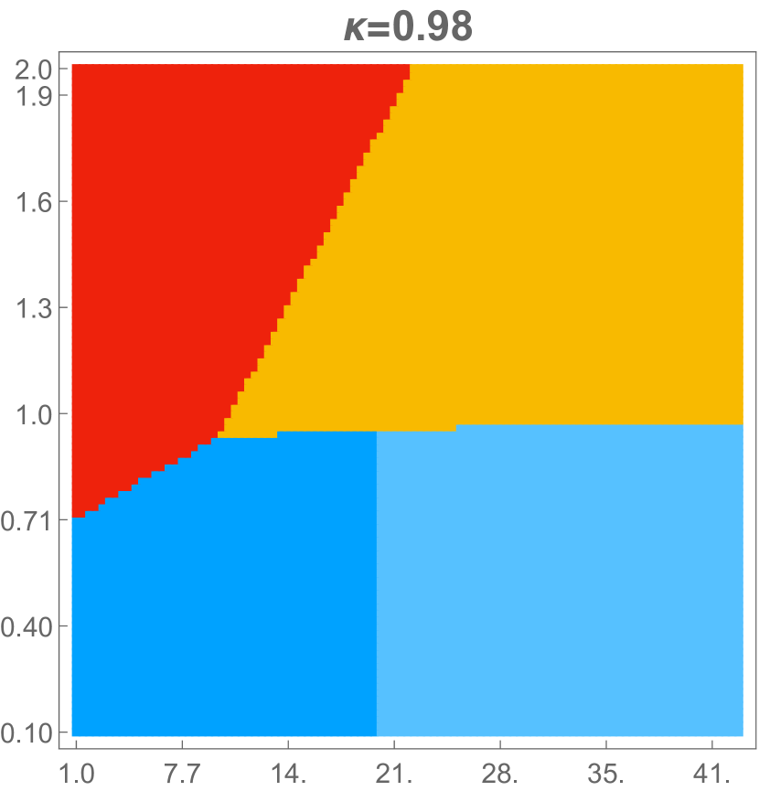
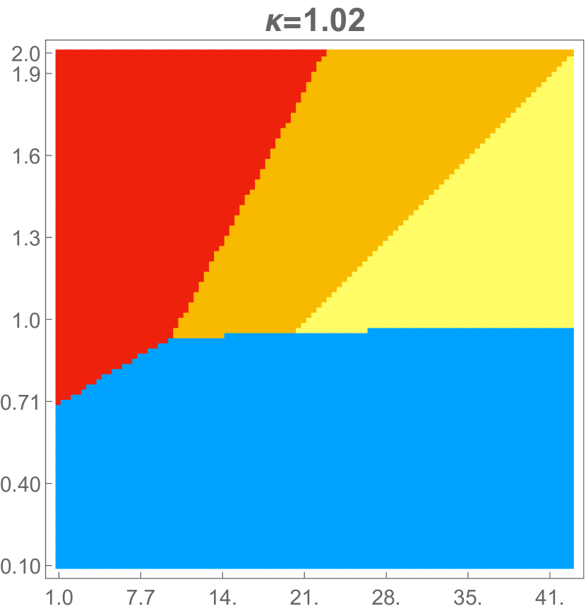
Figure 12: Phase diagrams for intermediate-tension walls exhibiting sweeping transitions. On the left a restpoint of the vacuum solution is swept away as $\gamma$ increases beyond a critical value. On the right the same happens in the warm solution but for decreasing $\gamma$. In these diagrams, the one-center warm solution is always [H1,E2].

Warm solutions of type [H1,E1], respectively [E1,H1], exist for tensions $\lambda>1/\ell_{1}\Longrightarrow\kappa>b$, respectively $\lambda>1/\ell_{2}\Longrightarrow\kappa>1$. In the case of a defect these two ranges coincide. The stable black hole forms in the larger of the two slices, i.e. for $\gamma>1$ in the $j=1$ slice. The sweeping transition occurs at the critical mass ratio $\mu_{2}^{*}=(b^{2}-\kappa^{2})^{-1}$, which through eqs. (6.11) and (6.12a) corresponds to a fixed value of $\tau_{2}$. Since $\tau=\tau_{2}(1+\gamma)$, the critical orange-yellow line is a straight line in the $(\gamma,\tau)$ plane, in accordance again with the findings of fig. 12.

A noteworthy fact is the rapidity of these transitions as function of $\kappa$. For $\kappa$ a little below or above the critical value the single-center cold, respectively warm phases almost disappear. Note also the cold-to-warm transitions are always near $\tau\approx 1$. This is the critical value for Hawking-Page transitions in the homogeneous case, as expected at large $\gamma$ when the $j=1$ slice covers most of space.

The critical curves for the cold-to-hot and warm-to-hot transitions also look linear in the above figures, but this is an illusion. Since the transitions are first order we must compare free energies. Equating for example the hot and cold free energies gives after some rearrangements (and with $\ell_{1}=\ell_{2}:=\ell$)

$$2\pi^{2}\tau+{2\over\ell}\log g_{I}={1\over 2\tau_{1}}|M_{1}|L_{1}^{2}\,(1+{\mu\over\gamma})\ .$$ (9.2)

Now $|M_{1}|L_{1}^{2}$ can be expressed in terms of $\mu$ through eq. (6.8, 6.9a), and $\mu$ in the cold phase is a function of $\gamma$. Furthermore $\log g_{I}/\ell=4\pi{\rm tanh}^{-1}(\kappa/2)$ is constant, see eq. (4.9), and $\tau_{1}=\tau/(1+\gamma^{-1})$. Thus (9.2) can be written as a relation $\tau=\tau_{\rm hc}(\gamma)$, and we have verified numerically that $\tau_{\rm hc}$ is not a linear function of $\gamma$.

9.2 Non-degenerate vacua

Figure 13 presents the phase diagram in the case of non-degenerate AdS vacua, $b=\ell_{2}/\ell_{1}=c_{2}/c_{1}=3$, and for different values of the tension in the allowed range, $\kappa\in(2,4)$. Since there is no $\gamma\to\gamma^{-1}$ symmetry, $\gamma$ here varies between 0 to $\infty$. To avoid squeezing the $\gamma\in(0,1)$ region, we use for horizontal axis $\alpha:=\gamma-\gamma^{-1}$. This is almost linear in the larger of $\gamma$ or $\gamma^{-1}$, when either of these is large, but the region $\gamma\approx 1$ is distorted compared to figs. 11 and 12 of the previous section.

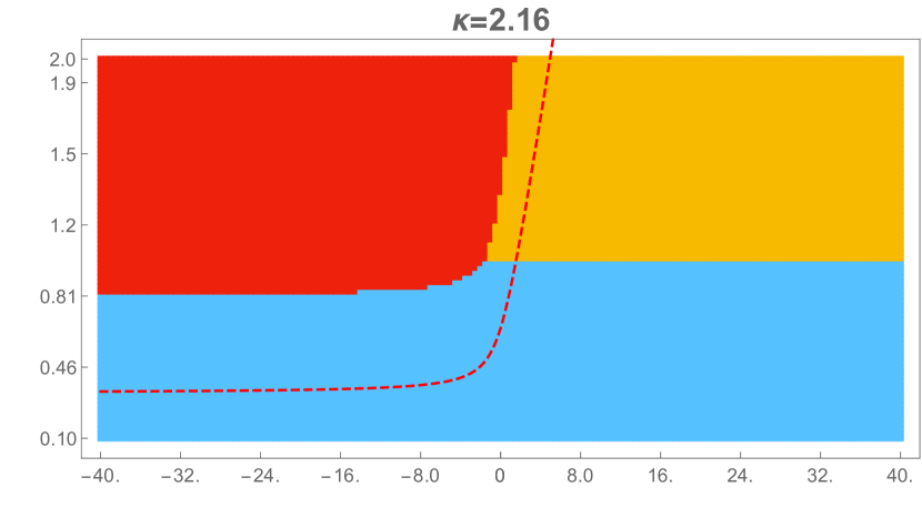
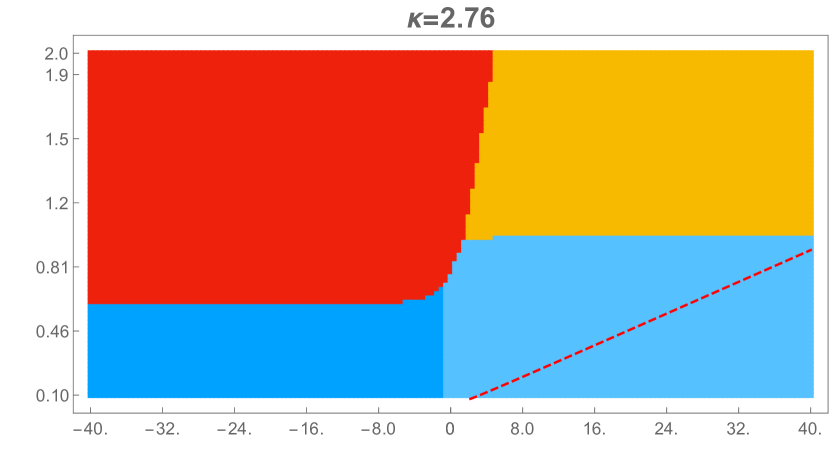
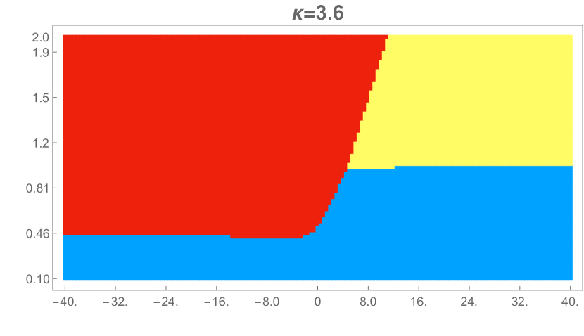
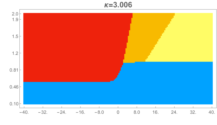
Figure 13: Phase diagrams for $b=3$, and values of the tension that increase from the top-left figure clockwise. The horizontal and vertical axes are $\alpha:=\gamma-\gamma^{-1}$ and $\tau$. The broken red curve is the bound $\tau=\tau_{2}^{*}(1+\gamma)$ below which the hot solution does not exist (there is no such bound in the lower panels in which the tension $\lambda>\lambda_{0}$)

. Note the absence of a warm phase in the left ($\gamma<1$) region of the diagrams. For the heaviest wall all non-hot solutions are double-center.

The most notable new feature in these phase diagrams is the absence of a warm phase in the region $\gamma<1$. This shows that it is impossible to keep the wall outside the black hole when the latter forms on the false-vacuum side. From the perspective of the dual ICFT, see section 7.1, the absence of [X,H1]-type solutions means that no interfaces, however heavy, can keep CFT₁ in the confined phase if CFT₂ (the theory with larger central charge) has already deconfined.

We suspect that this is a feature of the thin-brane model which does not allow interfaces to be perfectly-reflecting [34].

Warm solutions with the horizon in the pink slice appear to altogether disappear above the critical ratio of central charges $b_{c}=3$. The boundary conditions corresponding to topologies of type [X,H1] are given by eqs.  (6.14). We plotted the right-hand side of the second condition (6.14) for different values of $\lambda$ and $\mu$ in their allowed range, and found no solution with positive $\tau_{1}$ for $b>3$. Analytic evidence for the existence of a strict $b_{c}=3$ bound can be found by considering the limit of a maximally isolating wall, $\lambda\approx\lambda_{\rm max}$, and of a shrinking green slice $\hat{\mu}\to-\infty$. In this limit, the right-hand side of (6.14) can be computed in closed form with the result

$$\tau_{1}(\hat{\mu})={\pi\over\sqrt{-\hat{\mu}}}\biggl{(}2-\sqrt{1+{\ell_{2}\over\ell_{1}}}\,\,\biggr{)}+{\rm subleading}\ .$$ (9.3)

We took X=E1 as dictated by the analysis of sweeping transitions, see section 7.2 and in particular eq. (7.5). This limiting $\tau_{1}(\hat{\mu})$ is negative for $b>3$, and positive for $b<3$ where warm [E1,H1] solutions do exist, as claimed.

An interesting corollary is that end-of-the-world branes cannot avoid the horizon of a black hole, since the near-void limit, $\ell_{1}\ll\ell_{2}$, is in the range that has no [X,H1] solutions.

9.3 Unstable black holes

The phase diagrams in figs. 11, 12, 13 show the solution with the lowest free energy in various regions of parameter space. Typically, this dominant phase coexists with solutions that describe unstable or metastable black-holes which are ubiquitous in the thin-wall model.

Figure 14 shows the number of black hole solutions in the degenerate case, $b=1$, for small, intermediate and large wall tension, and in different regions of the $(\tau,\gamma)$ parameter space. The axes are the same as in figs. 11 and 12 but the range of $\gamma$ is halved. At sufficiently high temperature the growing horizon captures the wall, and the only solution is the hot solution. We see

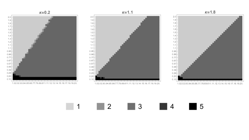
Figure 14: The number of independent black hole solutions in the $(\gamma,\tau)$ parameter space for $b=1$, and three values of the tension $(\kappa=0.2;\ 1.1;{\rm and}\ 1.8)$. The darker the shade the larger the number of black holes.

however that in a large region of intermediate temperatures the hot solution coexists with two warm solutions. Finally at very low temperature the hot solution coexists with four other black-hole solutions, two on either side of the wall. The dominant phase in this region is vacuum, so the black holes play no role in the canonical ensemble.

The hot solution exists almost everywhere, except when $\lambda<\lambda_{0}$ and $\tau=\tau_{2}(1+\gamma)<\tau_{2}^{*}(1+\gamma)$ with $\tau_{2}^{*}$ given by eq. (6.5). It has positive specific heat even when it is not the dominant phase. For warm black holes, on the other hand, the specific heat can have either sign. One can see this semi-analytically by focussing once again on our favourite near-critical region $\lambda\approx\lambda_{0}$. Simple inspection of fig. 8 shows that in some range $\tau_{2}^{*}<\tau_{2}<\tau_{2}^{\rm max}$ the hot solution coexists with two nearby warm solutions. At the maximum $\tau_{2}^{\rm max}$, where $d\tau_{2}/d\mu=0$, the warm solutions merge and then disappear. Since the black hole is in the $j=1$ slice, $M_{1}=(2\pi T)^{2}$ and their energy reads

$$E_{\rm[warm]}\,=\,{1\over 2}(\ell_{1}M_{1}L_{1}+\ell_{2}M_{2}L_{2})\,=\,2\pi^{2}T^{2}L_{2}\,\bigl{(}\ell_{1}\gamma+\ell_{2}{\mu}\,\bigr{)}\ .$$ (9.4)

Taking a derivative with respect to $T$ with $L_{1},L_{2}$ kept fixed we obtain

$${d\over dT}E_{\rm[warm]}\,=\,{2\over T}E_{\rm[warm]}+2\pi^{2}T^{2}\,L_{2}^{\,2}\,\ell_{2}\,{d\mu\over d\tau_{2}}\ .$$ (9.5)

Near $\tau_{2}^{\rm max}$ the dominant contribution to this expression comes from the derivative ${d\mu/d\tau_{2}}$ which jumps from $-\infty$ to $+\infty$. It follows that the warm black hole with the higher mass has negative specific heat, and should decay to its companion black hole either classically or in the quantum theory.

It would be very interesting to calculate this decay process, but we leave this for future work.

One last comment concerns transitions from the double-center vacuum geometries, of type [E1,E1], to warm solutions where the wall avoids the horizon. One can ask what side of the wall does the black hole choose. A natural guess is that it forms in the deepest of the two AdS wells. The relative depth is the ratio of blueshift factors at the two rest points,

$${\mathfrak{R}}:=\sqrt{g_{tt}|_{r_{1}=0}\over g_{tt}|_{r_{2}=0}}\,=\,{\ell_{2}\over\ell_{1}\sqrt{\mu(\gamma)}}\,\ .$$ (9.6)

One expects the black hole to form in the $j=1$ (green) slice if ${\mathfrak{R}}<1$ and in the $j=2$ (red) slice if ${\mathfrak{R}}>1$. Our numerical plots confirmed in all cases this expectation.

10 Outlook

One urgent question, already noted in the introduction, is how much of this analysis will survive in top-down interface models, where gravitating domain walls are typically thick. The order parameters of the Hawking-Page and sweeping transitions – the area of the horizon and the number of rest points for inertial observers, do not depend on the assumption of a thin wall and could go through. The warm-to-hot transition, on the other hand, may be replaced by a crossover, since there is no sharp criterion to decide if a thick wall enters or avoids the horizon. As discussed, however, in section 7.1 a sharp order parameter, such as a Polyakov loop, may be suggested by the field theory side of the correspondence.

One other question left open in the present work is the entanglement structure of the equilibrium states. Indeed, a guiding thread of our paper were the intersections of the domain wall with the black hole horizon and the trajectories of inertial observers. The Ryu-Takayanagi (RT) surfaces [58, 59] are another natural class of curves whose intersection with the wall should be studied along lines similar to ref. [21, 22] for BCFT.

Simple extensions of the minimal model, such as the addition of a Chern-Simons field (see e.g. [107]) might also be worth exploring.

Last but not least, the simplicity of the model and its rich spectrum of black holes make it a promising ground where to try to shed some more light on the recent exciting developments related to black hole evaporation, islands and the Page curve [12, 13, 14]. We hope to return to some of these questions in the near future.

Aknowledgements

We are grateful to Mark Van Raamsdonk for his critical reading of a preliminary draft of this paper and for many useful comments. Many thanks also to Panos Betzios, Shira Chapman, Dongsheng Ge, Elias Kiritsis, Ioannis Lavdas, Bruno Le Floch, Emil Martinec, Olga Papadoulaki and Giuseppe Policastro for discussions during the course of this work.

Appendix A Renormalized on-shell action

The Euclidean action of the holographic-interface model, in units $8\pi G=1$, is the sum of bulk, brane, boundary and corner contributions, see e.g.[108]

$$I_{\rm gr}=-\frac{1}{2} \hskip-7.11317pt\int_{{\mathbb{S}}_{1}}d^{3}x\sqrt{g_{1}}\,(R_{1}+\frac{2}{\ell_{1}^{2}})-\frac{1}{2}\int_{{\mathbb{S}}_{2}}d^{3}x\sqrt{g_{2}}\,(R_{2}+\frac{2}{\ell_{2}^{2}})+\lambda\int_{\mathbb{W}}d^{2}s\sqrt{\hat{g}_{w}}\ \ \ \ \ \$$ (A.1)

$$\hskip-17.07164pt+\int_{\partial{\mathbb{S}}_{1}}d^{2}s\sqrt{\hat{g}_{1}}\,K_{1}+\int_{\partial{\mathbb{S}}_{2}}d^{2}s\sqrt{\hat{g}_{2}}\,K_{2}\ +\ \int_{\rm C}(\theta-\pi)\sqrt{\hat{g}_{c}}+{\rm c.t.}\$$

where the counterterms, abbreviated above by c.t., read [109]

$${\rm c.t.}=\,{1\over\ell_{1}}\int_{{\rm B}_{1}}\sqrt{\hat{g}_{1}}\,+{1\over\ell_{2}}\int_{{\rm B}_{2}}\sqrt{\hat{g}_{2}}\,-\,\int_{{\rm B}_{1}\cap{\rm B}_{2}}(\theta_{1}+\theta_{2})\sqrt{\hat{g}_{c}}\ .$$ (A.2)

Here $\mathbb{S}_{j}$ are the spacetime slices whose boundary is the sum of the cutoff surface B_j and of the string worldsheet $\mathbb{W}$, i.e. $\partial\mathbb{S}_{j}=$B${}_{j}\cup\mathbb{W}$ . The induced metrics are denoted by hats. The $K_{j}$ are traces of the extrinsic curvatures on each slice computed with the inward-pointing normal vector. Finally, in addition to the standard Gibbons-Hawking-York boundary terms, one must add the Hayward term [110, 108] at corners of $\partial\mathbb{S}_{j}$ denoted by C.  There is at least one such corner at the cutoff surface, B${}_{1}\cap$B₂, where $\theta-\pi$ is the sum of the angles $\theta_{j}$ defined in figure 4.

Let us break the action into an interior and a conformal boundary term, $I_{\rm gr}=I_{\rm int}+I_{\rm B}$, with the former including contributions from the worldsheet W. Using the field equations $R_{j}=-{6/\ell_{j}^{2}}$ and $K_{1}|_{\rm W}+K_{2}|_{\rm W}=-2\lambda$, and the volume elements that follow from eqs. (3.1) and (4.1, 4.2),

$$\sqrt{g_{j}}\,d^{3}x=\ell_{j}r_{i}dr_{j}dx_{j}dt\,\quad{\rm and}\quad\,\sqrt{\hat{g}_{w}}\,d^{2}s=\sqrt{fg}\,d\sigma dt\ ,$$

we can write the interior on-shell action as follows :

$$I_{\rm int}\,=\,\frac{2}{\ell_{1}}\int_{{\Omega}_{1}}r_{1}\,dr_{1}dx_{1}dt+\frac{2}{\ell_{2}}\int_{{\Omega}_{2}}r_{2}\,dr_{2}dx_{2}dt-\lambda\int_{\mathbb{W}}\sqrt{fg}\,d\sigma dt\ .$$ (A.3)

We have been careful to distinguish the spacetime slice S_j from the coordinate chart $\Omega_{j}$, because we will now use Stoke’s theorem treating $\Omega_{j}$ as part of flat Euclidean space,

$$\sum_{j=1,2}\,{2\over\ell_{j}}\int_{{\Omega}_{j}}r_{j}dr_{j}dx_{j}dt\ =\ \sum_{j=1,2}\,{1\over\ell_{j}}\oint_{{\partial\Omega}_{j}}r_{j}^{2}(\hat{r}_{j}\cdot d\hat{n}_{j})dt\ ,$$ (A.4)

with $d\hat{n}_{j}dt$ the surface element on the boundary $\partial\Omega_{j}$. Crucially, the boundary of $\Omega_{j}$ may include a horizon which is a regular interior submanifold of the Euclidean spacetime and is not therefore part of $\partial\mathbb{S}_{j}$ . In particular, there is no Gibbons-Hawking-York contribution there.

The boundary integral in eq. (A.4) receives contributions from the three pieces of ${\partial\Omega}_{1,2}$ : the cutoff surface B${}_{1}\cup$B₂, the horizon if there is one, and the worldsheet $\mathbb{W}$. Conveniently, this last term precisely cancels the third term in (A.3) by virtue of the Israel-Lanczos equation (4.3). Thus, after all the dust has settled, the action can be written as the sum of terms evaluated either at the black-hole horizon or at the cutoff. After integrating over periodic time the interior part of the action, eq. (A.3) , reads

$$I_{\rm int}\,=\ {1\over\ell_{1}T}\,\Bigl{[}r_{1}^{2}\,\Delta x_{1}\Bigr{]}_{\rm Hor}^{{\rm B}_{1}}+\,{1\over\ell_{2}T}\,\Bigl{[}r_{2}^{2}\,\Delta x_{2}\Bigr{]}_{\rm Hor}^{{\rm B}_{2}}$$ (A.5)

where we employ the shorthand notation $[X]_{a}^{b}=X|_{b}-X|_{a}$ , and $X|_{a}$ for $X$ evaluated at $a$ . If the slice $\mathbb{S}_{j}$ does not contain a horizon the corresponding contribution is absent.

We now turn to the conformal-boundary contributions from the lower line in the action (A.1). For a fixed-$r_{j}$ surface, the inward-pointing unit normal expressed as a 1-form is n${}_{j}=-dr_{j}/\sqrt{r_{j}^{2}-M_{j}\ell_{j}^{2}}$ . One finds after a little algebra (we here drop the index $j$ for simplicity)

$$K_{xx}=K_{tt}=-{r\over\ell}\sqrt{r^{2}-M\ell^{2}}\,\Longrightarrow\,\sqrt{\hat{g}}\,K=\,-{1\over\ell}(2r^{2}-M\ell^{2})\ .$$ (A.6)

Combining the Gibbons-Hawking-York terms and the counterterms gives

$$I_{\rm B}={1\over\ell_{1}T}(r_{1}\sqrt{r_{1}^{2}-M_{1}\ell_{1}^{2}}-2r_{1}^{2}+M_{1}\ell_{1}^{2})\,\Delta x_{1}\,\Bigl{|}_{{\rm B}_{1}}\,+\,(1\rightarrow 2)\ .$$ (A.7)

Expanding for large cutoff radius, $r_{j}|_{{\rm B}_{j}}\to\infty$, and dropping the terms that vanish in the limit we obtain

$$I_{\rm B}={1\over\ell_{1}T}(-r_{1}^{2}+{1\over 2}M_{1}\ell_{1}^{2})\,\Delta x_{1}\,\Bigl{|}_{{\rm B}_{1}}\,+\,(1\rightarrow 2)\ .$$ (A.8)

Upon adding up (A.5) and (A.8) the leading divergent term cancels, giving the following result for the renormalized on-shell action :

$$I_{\rm gr}\ =\ {M_{1}\ell_{1}\over 2T}\bigl{(}L_{1}-2\Delta x_{1}\bigl{|}_{{\rm Hor}}\bigr{)}\,+\,{M_{2}\ell_{2}\over 2T}\bigl{(}L_{2}-2\Delta x_{2}\bigl{|}_{{\rm Hor}}\bigr{)}\,\ .$$ (A.9)

We used here the fact that $\Delta x_{j}|_{{\rm B}_{j}}=L_{j}$, and that $r_{j}^{2}=M_{j}\ell_{j}^{2}$ at the horizon when one exists. We also used implicitly the fact that for smooth strings the Hayward term receives no contribution from the interior and is removed by the counterterm at the boundary.

As a check of this on-shell action let us compute the entropy. Using our formula for the internal energy $\langle E\rangle={1\over 2}(M_{1}\ell_{1}L_{1}+M_{2}\ell_{2}L_{2})$, see section 2, and $I_{\rm gr}=\langle E\rangle/T-S$ we find

$$S={1\over T} \hskip-28.45274pt\bigl{(}M_{1}\ell_{1}\Delta x_{1}\bigl{|}_{{\rm Hor}}+M_{2}\ell_{2}\Delta x_{2}\bigl{|}_{{\rm Hor}}\bigr{)}$$ (A.10)

$$= \hskip-5.69054pt4\pi^{2}T\bigl{(}\ell_{1}\Delta x_{1}\bigl{|}_{{\rm Hor}}+\ell_{2}\Delta x_{2}\bigl{|}_{{\rm Hor}}\bigr{)}\,=\,{A({\rm horizon})\over 4G}\ .$$

In the lower line we used the fact that $M_{j}=(2\pi T)^{2}$ and $r_{j}^{\rm H}=2\pi T\ell_{j}$ for slices with horizon, plus our choice of units $8\pi G=1$. The calculation thus reproduces correctly the Bekenstein-Hawking entropy.

Appendix B Opening arcs as elliptic integrals

In this appendix we express the opening arcs, eqs. (4.17), in terms of complete elliptic integrals of the first, second and third kind,

$${\rm\bf K}(\nu)=\int_{0}^{1}\frac{dy}{\sqrt{(1-y^{2})(1-\nu y^{2})}}$$ (B.1)

$${\bf E}(\nu)=\int_{0}^{1}\frac{\sqrt{1-\nu y^{2}}\,dy}{\sqrt{1-y^{2}}}\ .$$ (B.2)

$${\bf\Pi}(u,\nu)=\int_{0}^{1}\frac{dy}{(1-uy^{2})\sqrt{(1-y^{2})(1-\nu y^{2})}}\ .$$ (B.3)

Consider the boundary conditions (4.17a). The other conditions (4.17b, 4.17c) differ only by the constant periods or horizon arcs, $P_{j}$ or $\Delta x_{j}|_{\rm hor}$. Inserting the expression (4.16) for $x_{1}^{\prime}$ gives

$$L_{1}=-\int_{\sigma_{+}}^{\infty}\frac{\ell_{1}\,d\sigma}{(\sigma+M_{1}\ell_{1}^{2})}\,\frac{(\lambda^{2}+\lambda_{0}^{2})\,\sigma+M_{1}-M_{2}}{\sqrt{A\sigma(\sigma-\sigma_{+})(\sigma-\sigma_{-})}}\ ,$$ (B.4)

and likewise for $L_{2}$. The roots $\sigma_{\pm}$ are given by eqs. (4.14, 4.15). We assume that we are not in the case [H2, H2] where $M_{1}=M_{2}>0$, nor in the fringe case $\sigma_{+}=-M_{j}\ell_{j}^{2}$ when the string goes through an AdS center. These cases will be treated separately.

Separating the integral in two parts, and trading the integration variable $\sigma$ for $y$, with $y^{2}:=\sigma_{+}/\sigma$, we obtain

$$L_{1}=-\frac{2\ell_{1}}{\sqrt{A\,\sigma_{+}}}\bigg{[}{M_{1}-M_{2}\over M_{1}\ell_{1}^{2}}\int_{0}^{1}\frac{dy}{\sqrt{(1-y^{2})(1-\nu y^{2})}}$$

$$+\Bigl{(}(\lambda^{2}+\lambda_{0}^{2})-{M_{1}-M_{2}\over M_{1}\ell_{1}^{2}}\Bigr{)}\,\int_{0}^{1}\frac{y^{2}dy}{(1-u_{1}y^{2})\sqrt{(1-y^{2})(1-\nu y^{2})}}\,\bigg{]}\ \ \$$ (B.5)

where $\nu=\sigma_{-}/\sigma_{+}$ and $u_{1}=-M_{1}\ell_{1}^{2}/\sigma_{+}$ . Identifying the elliptic integrals finally gives

$$L_{1}=-\frac{2\ell_{1}}{\sqrt{A\,\sigma_{+}}}\bigg{[}\frac{M_{1}-M_{2}}{M_{1}\ell_{1}^{\,2}}\,\Bigl{(}{\rm\bf K}(\nu)-{\bf\Pi}(u_{1},\nu)\Bigr{)}+(\lambda^{2}+\lambda_{0}^{2})\,{\bf\Pi}(u_{1},\nu)\bigg{]}\ ,\ \ \$$ (B.6)

and a corresponding expression for $L_{2}$

$$L_{2}=-\frac{2\ell_{2}}{\sqrt{A\,\sigma_{+}}}\bigg{[}\frac{M_{2}-M_{1}}{M_{2}\ell_{2}^{\,2}}\,\Bigl{(}{\rm\bf K}(\nu)-{\bf\Pi}(u_{2},\nu)\Bigr{)}+(\lambda^{2}-\lambda_{0}^{2})\,{\bf\Pi}(u_{2},\nu)\bigg{]}\ \ \$$ (B.7)

with $u_{2}=-M_{2}\ell_{2}^{2}/\sigma_{+}$ . The prefactors in (B.6) diverge when $M_{1}\to 0$ but the singilarity is removed by expanding ${\bf\Pi}(u_{1},\nu)$ around $u_{1}=0$. In this limit

$$L_{1}(M_{1}=0)=-\frac{2\ell_{1}}{\sqrt{A\,\sigma_{+}}}\bigg{[}\frac{M_{2}}{\sigma_{-}}({\rm\bf E}(\nu)-{\rm\bf K}(\nu))+(\lambda^{2}+\lambda_{0}^{2}){\rm\bf K}(\nu)\bigg{]}$$ (B.8a)

and similarly

$$L_{2}(M_{2}=0)=-\frac{2\ell_{2}}{\sqrt{A\,\sigma_{+}}}\bigg{[}\frac{M_{1}}{\sigma_{-}}({\rm\bf E}(\nu)-{\rm\bf K}(\nu))+(\lambda^{2}-\lambda_{0}^{2}){\rm\bf K}(\nu)\bigg{]}$$ (B.8b)

with ${\rm\bf E}(\nu)$ the complete elliptic integral of the second kind.

The $M_{1}=M_{2}>0$ geometries correspond to the high-temperature phase where $M_{j}=(2\pi T)^{2}$, $\sigma_{+}=0$ and $\sigma_{-}=-(4\pi T\lambda)^{2}/A$. The integrals (4.17c) simplify to elementary functions in this case:

$$L_{1}-\Delta_{1}^{\rm Hor}\ =\ -{\ell_{1}(\lambda^{2}+\lambda_{0}^{2})\over\sqrt{A\,|\sigma_{-}|\,}}\underbrace{\int_{0}^{\infty}{ds\over(s+a)\,\sqrt{s+1}\,}}_{\textstyle\begin{array}[]{c}={2\over\sqrt{1-a}}{\rm arctanh}({\sqrt{1-a}})\end{array}}$$

with $a=A\ell_{1}^{2}/4\lambda^{2}$. Using the expression (4.14) for $A$, and going through the same steps for $j=2$, gives after a little algebra

$$L_{1}-\Delta_{1}^{\rm Hor}\ =\ -{1\over\pi T}\,{\rm tanh}^{-1}\left({\ell_{1}(\lambda^{2}+\lambda^{2}_{0})\over 2\lambda}\right)\ ,$$ (B.9a)

$$L_{2}-\Delta_{2}^{\rm Hor}\ =\ -{1\over\pi T}\,{\rm tanh}^{-1}\left({\ell_{2}(\lambda^{2}-\lambda^{2}_{0})\over 2\lambda}\right)\ .$$ (B.9b)

Interestingly, since $\Delta_{2}^{\rm Hor}$ must be positive, $TL_{2}$ is bounded from below in the range $\lambda<\lambda_{0}$ as discussed in section 6.2.

In the high-temperature phase the on-shell action, eq. (A.9), reads

$$I_{\rm gr}^{\rm(high-T)}=4\pi^{2}T\Bigl{[}-{1\over 2}(\ell_{1}L_{1}+\ell_{2}L_{2})+\ell_{1}(L_{1}-\Delta_{1}^{\rm Hor})+\ell_{2}(L_{2}-\Delta_{2}^{\rm Hor})\Bigr{]}\,.\ \$$ (B.10)

Using the expressions (B.9) and rearranging the arc-tangent functions gives

$$I_{\rm gr}^{\rm(high-T)}:={E\over T}-S=-2\pi^{2}T(\ell_{1}L_{1}+\ell_{2}L_{2})-\log\,g_{I}$$ (B.11)

where the interface entropy $S=\log\,g_{I}$ is given by eq. (4.9).

Appendix C Sweeping is continuous

In this appendix we show that sweeping transitions are continuous.

We focus for definiteness on the sweeping of the $j=2$ AdS center at zero temperature (all other cases work out the same). The transition takes place when $\mu$ crosses the critical value $\mu_{2}^{*}$ given by eq. (7.2). Setting $\mu=\mu_{2}^{*}(1-\delta)$ in expression (6.9b) gives

$$f_{2}(\mu)=\,\frac{\ell_{2}}{\sqrt{A}}\int_{s_{+}}^{\infty}ds\,\frac{(\lambda^{2}-\lambda_{0}^{2})(s-\mu\ell_{2}^{2})\,+\delta}{(s-\mu\ell_{2}^{2})\,\sqrt{As(s-s_{+})(s-s_{-})}}$$

$$=\,\frac{2\ell_{2}(\lambda^{2}-\lambda_{0}^{2})}{\sqrt{As_{+}}}\,{\bf K}\bigl{(}\frac{s_{-}}{s_{+}}\bigr{)}\,+\,\frac{\ell_{2}\,\delta}{\sqrt{A}}\,\underbrace{\int_{s_{+}}^{\infty}\frac{ds}{(s-\mu\ell_{2}^{2})\sqrt{s(s-s_{+})(s-s_{-})}}}_{J}\ .\ \$$ (C.1)

The first term is continuous at $\delta=0$, but the second requires some care because the integral $J$ diverges. This is because for small $\delta$

$$s_{+}-\mu\ell_{2}^{2}\,=\,\frac{\delta^{2}}{4\lambda^{2}\mu_{2}^{*}}+\mathcal{O}(\delta^{3})\ ,$$ (C.2)

as one finds by explicit computation of the expression (6.10). If we set $\delta=0$, $J$ diverges near the lower integration limit. To bring the singular behavior to $0$ we perform the change of variable $u^{2}=s-s_{+}$, so that

$$J=\int_{0}^{\infty}\frac{2du}{(u^{2}+\delta^{2}/4\lambda^{2}\mu_{2}^{*})\sqrt{(u^{2}+s_{+}^{*})(u^{2}+s_{+}^{*}-s_{-}^{*})}}\ ,$$ (C.3)

where we kept only the leading order in $\delta$, and $s_{\pm}^{*}$ are the roots at $\mu=\mu_{2}^{*}$. Since $s_{+}^{*}$ and $s_{+}^{*}-s_{-}^{*}$ are positive and finite, the small-$\delta$ behavior of the integral is (after rescaling appropriately $u$)

$$J={4\lambda|\mu_{2}^{*}|\over|\delta|\sqrt{s_{+}^{*}(s_{+}^{*}-s_{-}^{*})}}\,\underbrace{\int_{0}^{\infty}{du\over u^{2}+1}}_{\pi/2}\ +\ {\rm finite}\ .$$ (C.4)

Inserting in expression  (C.1) and doing some tedious algebra leads finally to a discontinuity of the function $f_{2}(\mu)$ equal to sign$(\delta)\,\pi/\sqrt{\mu_{2}^{*}}$ . This is precisely what is required for $L_{2}$, eq. (6.8), to be continuous when the red ($j=2$) slice goes from type E1 at negative $\delta$ to type E2 at positive $\delta$.

Appendix D Bubbles exist

We show here that the bubble phenomenon of section 8 is indeed realized in a region of the parameter space of the holographic model.

This is the region of non-degenerate gravitational vacua ($\ell_{2}$ strictly bigger than $\ell_{1}$) and a sufficiently light domain wall. Specifically, we will show that for $\lambda$ close to its minimal value, $\lambda_{\rm min}$, the arc $L_{1}(\mu=0)$ is negative, so the wall self-intersects and $\mu_{0}$ is necessarily finite.

Let $\lambda=\lambda_{\rm min}(1+\delta)$ with $\delta\ll 1$. Setting $\mu=0$ and expanding eqs. (6.10) for small $\delta$ gives

$$A={8\lambda_{\rm min}^{2}\,\delta\over\ell_{1}\ell_{2}}+\mathcal{O}(\delta^{2})\ ,\quad s_{+}={\ell_{2}\over 4\lambda_{\rm min}}+\mathcal{O}(\delta)\ ,\quad s_{-}=-{\ell_{1}\over\ 2\lambda_{\rm min}\delta}+\mathcal{O}(1)\ .$$

Plugging into eq. (B.6) with $M_{2}=\mu M_{1}\approx 0$ we find :

$$\sqrt{|M_{1}|}\,L_{1}=-\frac{2}{\ell_{1}\sqrt{As_{+}}}\left[{\bf K}\left({s_{-}\over s_{+}}\right)+(1-\frac{2\ell_{1}}{\ell_{2}}){\bf\Pi}\left({\ell_{1}^{2}\over s_{+}},\,{s_{-}\over s_{+}}\right)\right]$$ (D.1)

where we have only kept leading orders in $\delta$. Now we need the asymptotic form of the elliptic integrals when their argument diverges

$${\bf K}\left[-\frac{a}{\delta}\right]\approx{\bf\Pi}\left[u,-\frac{a}{\delta}\right]\approx-\frac{\ln(\delta)\sqrt{\delta}}{2\sqrt{a}}+\mathcal{O}(\sqrt{\delta})$$ (D.2)

for $\delta\to 0_{+}$ with $u,a$ fixed. Using $a=2\ell_{1}/\ell_{2}$ finally gives

$$\sqrt{|M_{1}|}\,L_{1}\,\approx\,\bigl{(}\frac{\ell_{2}}{\ell_{1}}-1\bigr{)}^{1/2}\ln(\delta)\,+\,{\rm subleading}\ .$$ (D.3)

For $\delta\ll 1$ this is negative, proving our claim. Note that we took the green slice to be of type E2, as follows from our analysis of the sweeping transitions for light domain walls – see section 7.2.

References

- [1] S. R. Coleman and F. De Luccia, “Gravitational Effects on and of Vacuum Decay,” Phys. Rev. D 21 (1980), 3305
- [2] L. Randall and R. Sundrum, “An Alternative to compactification,” Phys. Rev. Lett. 83 (1999), 4690-4693 [hep-th/9906064].
- [3] G. R. Dvali, G. Gabadadze and M. Porrati, “4-D gravity on a brane in 5-D Minkowski space,” Phys. Lett. B 485 (2000), 208-214 [hep-th/0005016].
- [4] A. Karch and L. Randall, “Locally localized gravity,” JHEP 05 (2001), 008 [hep-th/0011156].
- [5] A. Karch and L. Randall, “Open and closed string interpretation of SUSY CFT’s on branes with boundaries,” JHEP 06 (2001), 063 [hep-th/0105132].
- [6] O. DeWolfe, D. Z. Freedman and H. Ooguri, “Holography and defect conformal field theories,” Phys. Rev. D 66 (2002), 025009 [hep-th/0111135].
- [7] C. Bachas, J. de Boer, R. Dijkgraaf and H. Ooguri, “Permeable conformal walls and holography,” JHEP 06 (2002), 027 [hep-th/0111210].
- [8] B. Freivogel, V. E. Hubeny, A. Maloney, R. C. Myers, M. Rangamani and S. Shenker, “Inflation in AdS/CFT,” JHEP 03 (2006), 007 [hep-th/0510046].
- [9] B. Freivogel, G. T. Horowitz and S. Shenker, “Colliding with a crunching bubble,” JHEP 05 (2007), 090 [hep-th/0703146].
- [10] J. L. F. Barbon and E. Rabinovici, “Holography of AdS vacuum bubbles,” JHEP 04 (2010), 123 [arXiv:1003.4966 [hep-th]].
- [11] S. Banerjee, U. Danielsson, G. Dibitetto, S. Giri and M. Schillo, “Emergent de Sitter Cosmology from Decaying Anti–de Sitter Space,” Phys. Rev. Lett. 121 (2018) no.26, 261301 [arXiv:1807.01570 [hep-th]].
- [12] G. Penington, “Entanglement Wedge Reconstruction and the Information Paradox,” JHEP 09 (2020), 002 [arXiv:1905.08255 [hep-th]].
- [13] A. Almheiri, N. Engelhardt, D. Marolf and H. Maxfield, “The entropy of bulk quantum fields and the entanglement wedge of an evaporating black hole,” JHEP 12 (2019), 063 [arXiv:1905.08762 [hep-th]].
- [14] A. Almheiri, R. Mahajan, J. Maldacena and Y. Zhao, “The Page curve of Hawking radiation from semiclassical geometry,” JHEP 03 (2020), 149 [arXiv:1908.10996 [hep-th]].
- [15] M. Rozali, J. Sully, M. Van Raamsdonk, C. Waddell and D. Wakeham, “Information radiation in BCFT models of black holes,” JHEP 05 (2020), 004 [arXiv:1910.12836 [hep-th]].
- [16] V. Balasubramanian, A. Kar, O. Parrikar, G. Sárosi and T. Ugajin, “Geometric secret sharing in a model of Hawking radiation,” [arXiv:2003.05448 [hep-th]].
- [17] H. Z. Chen, R. C. Myers, D. Neuenfeld, I. A. Reyes and J. Sandor, “Quantum Extremal Islands Made Easy, Part I: Entanglement on the Brane,” JHEP 10 (2020), 166 [arXiv:2006.04851 [hep-th]].
- [18] D. Bak, C. Kim, S. H. Yi and J. Yoon, “Unitarity of Entanglement and Islands in Two-Sided Janus Black Holes,” JHEP 01 (2021), 155 [arXiv:2006.11717 [hep-th]].
- [19] R. Emparan, A. M. Frassino and B. Way, “Quantum BTZ black hole,” JHEP 11 (2020), 137 [arXiv:2007.15999 [hep-th]].
- [20] H. Z. Chen, R. C. Myers, D. Neuenfeld, I. A. Reyes and J. Sandor, “Quantum Extremal Islands Made Easy, Part II: Black Holes on the Brane,” JHEP 12 (2020), 025 [arXiv:2010.00018 [hep-th]].
- [21] I. Akal, Y. Kusuki, N. Shiba, T. Takayanagi and Z. Wei, “Entanglement entropy in holographic moving mirror and Page curve,” [arXiv:2011.12005 [hep-th]].
- [22] F. Deng, J. Chu and Y. Zhou, “Defect extremal surface as the holographic counterpart of Island formula,” [arXiv:2012.07612 [hep-th]].
- [23] H. Geng, A. Karch, C. Perez-Pardavila, S. Raju, L. Randall, M. Riojas and S. Shashi, “Information Transfer with a Gravitating Bath,” [arXiv:2012.04671 [hep-th]].
- [24] J. D. Brown and C. Teitelboim, “Neutralization of the Cosmological Constant by Membrane Creation,” Nucl. Phys. B 297 (1988), 787-836
- [25] H. Ooguri and T. Takayanagi, “Cobordism Conjecture in AdS,” [arXiv:2006.13953 [hep-th]].
- [26] S. Lanza, F. Marchesano, L. Martucci and I. Valenzuela, “Swampland Conjectures for Strings and Membranes,” [arXiv:2006.15154 [hep-th]]. [arXiv:2006.15154 [hep-th]].
- [27] A. Bedroya, M. Montero, C. Vafa and I. Valenzuela, “de Sitter Bubbles and the Swampland,” [arXiv:2008.07555 [hep-th]]. [arXiv:2008.07555 [hep-th]].
- [28] S. W. Hawking and D. N. Page, “Thermodynamics of Black Holes in anti-De Sitter Space,” Commun. Math. Phys. 87 (1983), 577.
- [29] P. Simidzija and M. Van Raamsdonk, “Holo-ween,” JHEP 12 (2020), 028 [arXiv:2006.13943 [hep-th]].
- [30] Z. Fu and D. Marolf, “Bag-of-gold spacetimes, Euclidean wormholes, and inflation from domain walls in AdS/CFT,” JHEP 11 (2019), 040 [arXiv:1909.02505 [hep-th]].
- [31] A. May and M. Van Raamsdonk, “Interpolating between multi-boundary wormholes and single-boundary geometries in holography,” [arXiv:2011.14258 [hep-th]].
- [32] J. D. Brown and M. Henneaux, “Central charges in the canonical realization of asymptotic symmetries: an example from three-dimensional gravity,” Commun. Math. Phys. 104, 207 (1986).
- [33] T. Azeyanagi, A. Karch, T. Takayanagi and E. G. Thompson, “Holographic calculation of boundary entropy,” JHEP 03 (2008), 054 [arXiv:0712.1850 [hep-th]].
- [34] C. Bachas, S. Chapman, D. Ge and G. Policastro, “Energy Reflection and Transmission at 2D Holographic Interfaces,” Phys. Rev. Lett. 125 (2020) no.23, 231602 [arXiv:2006.11333 [hep-th]].
- [35] D. Bak, M. Gutperle and S. Hirano, “A Dilatonic deformation of AdS(5) and its field theory dual,” JHEP 05 (2003), 072 [hep-th/0304129].
- [36] J. Gomis and C. Romelsberger, “Bubbling Defect CFT’s,” JHEP 08 (2006), 050 [hep-th/0604155].
- [37] O. Lunin, “1/2-BPS states in M theory and defects in the dual CFTs,” JHEP 10 (2007), 014 [arXiv:0704.3442 [hep-th]].
- [38] E. D’Hoker, J. Estes and M. Gutperle, “Exact half-BPS Type IIB interface solutions. I. Local solution and supersymmetric Janus,” JHEP 06 (2007), 021 [arXiv:0705.0022 [hep-th]].
- [39] E. D’Hoker, J. Estes and M. Gutperle, “Exact half-BPS Type IIB interface solutions. II. Flux solutions and multi-Janus,” JHEP 06 (2007), 022 [arXiv:0705.0024 [hep-th]].
- [40] E. D’Hoker, J. Estes, M. Gutperle and D. Krym, “Exact Half-BPS Flux Solutions in M-theory. I: Local Solutions,” JHEP 08 (2008), 028 [arXiv:0806.0605 [hep-th]].
- [41] E. D’Hoker, J. Estes, M. Gutperle and D. Krym, “Janus solutions in M-theory,” JHEP 06 (2009), 018 [arXiv:0904.3313 [hep-th]].
- [42] M. Chiodaroli, M. Gutperle, L. Y. Hung and D. Krym, “String Junctions and Holographic Interfaces,” Phys. Rev. D 83 (2011), 026003 [arXiv:1010.2758 [hep-th]]
- [43] M. Chiodaroli, E. D’Hoker, Y. Guo and M. Gutperle, “Exact half-BPS string-junction solutions in six-dimensional supergravity,” JHEP 12 (2011), 086 [arXiv:1107.1722 [hep-th]]. .
- [44] C. Bachas and J. Estes, “Spin-2 spectrum of defect theories,” JHEP 06 (2011), 005 [arXiv:1103.2800 [hep-th]].
- [45] O. Aharony, L. Berdichevsky, M. Berkooz and I. Shamir, “Near-horizon solutions for D3-branes ending on 5-branes,” Phys. Rev. D 84 (2011), 126003 [arXiv:1106.1870 [hep-th]].
- [46] B. Assel, C. Bachas, J. Estes and J. Gomis, “Holographic Duals of D=3 N=4 Superconformal Field Theories,” JHEP 08 (2011), 087 [arXiv:1106.4253 [hep-th]].
- [47] D. Bak, M. Gutperle and R. A. Janik, “Janus Black Holes,” JHEP 10 (2011), 056 [arXiv:1109.2736 [hep-th]].
- [48] N. Bobev, K. Pilch and N. P. Warner, “Supersymmetric Janus Solutions in Four Dimensions,” JHEP 06 (2014), 058 [arXiv:1311.4883 [hep-th]].
- [49] C. Bachas, E. D’Hoker, J. Estes and D. Krym, “M-theory Solutions Invariant under ,” Fortsch. Phys. 62 (2014), 207-254 [arXiv:1312.5477 [hep-th]].
- [50] E. D’Hoker, M. Gutperle and C. F. Uhlemann, “Warped in Type IIB supergravity II: Global solutions and five-brane webs,” JHEP 05 (2017), 131 [arXiv:1703.08186 [hep-th]].
- [51] Y. Lozano, N. T. Macpherson, C. Nunez and A. Ramirez, “AdS3 solutions in massive IIA, defect CFTs and T-duality,” JHEP 12 (2019), 013 [arXiv:1909.11669 [hep-th]].
- [52] Y. Lozano, C. Nunez, A. Ramirez and S. Speziali, “-strings and AdS3 solutions to M-theory with small supersymmetry,” JHEP 08 (2020), 118 [arXiv:2005.06561 [hep-th]].
- [53] I. Arav, K. C. M. Cheung, J. P. Gauntlett, M. M. Roberts and C. Rosen, “Superconformal RG interfaces in holography,” JHEP 11 (2020), 168 [arXiv:2007.07891 [hep-th]].
- [54] M. Billò, V. Gonçalves, E. Lauria and M. Meineri, “Defects in conformal field theory,” JHEP 04 (2016), 091 [arXiv:1601.02883 [hep-th]].
- [55] A. R. Brown and A. Dahlen, “On ’nothing’ as an infinitely negatively curved spacetime,” Phys. Rev. D 85 (2012), 104026 [arXiv:1111.0301 [hep-th]].
- [56] T. Takayanagi, “Holographic Dual of BCFT,” Phys. Rev. Lett. 107 (2011), 101602 [arXiv:0712.1850 [hep-th]].
- [57] M. Fujita, T. Takayanagi and E. Tonni, “Aspects of AdS/BCFT,” JHEP 11 (2011), 043 [arXiv:1108.5152 [hep-th]].
- [58] S. Ryu and T. Takayanagi, “Holographic derivation of entanglement entropy from AdS/CFT,” Phys. Rev. Lett. 96 (2006), 181602 [arXiv:hep-th/0603001 [hep-th]].
- [59] S. Ryu and T. Takayanagi, “Aspects of Holographic Entanglement Entropy,” JHEP 08 (2006), 045 [arXiv:hep-th/0605073 [hep-th]].
- [60] B. Czech, J. L. Karczmarek, F. Nogueira and M. Van Raamsdonk, “The Gravity Dual of a Density Matrix,” Class. Quant. Grav. 29 (2012), 155009 [arXiv:1204.1330 [hep-th]].
- [61] A. C. Wall, “Maximin Surfaces, and the Strong Subadditivity of the Covariant Holographic Entanglement Entropy,” Class. Quant. Grav. 31 (2014) no.22, 225007 [arXiv:1211.3494 [hep-th]].
- [62] M. Headrick, V. E. Hubeny, A. Lawrence and M. Rangamani, “Causality \& holographic entanglement entropy,” JHEP 12 (2014), 162 [arXiv:1408.6300 [hep-th]].
- [63] M. Van Raamsdonk, “Lectures on Gravity and Entanglement,” [arXiv:1609.00026 [hep-th]].
- [64] M. Rangamani and T. Takayanagi, “Holographic Entanglement Entropy,” Lect. Notes Phys. 931 (2017), pp.1-246 [arXiv:1609.01287 [cond-mat.str-el]].
- [65] C. Bachas and I. Brunner, “Fusion of conformal interfaces,” JHEP 02 (2008), 085 [arXiv:0712.0076 [hep-th]].
- [66] E. Witten, “Deformations of JT Gravity and Phase Transitions,” [arXiv:2006.03494 [hep-th]].
- [67] M. Banados, “Three-dimensional quantum geometry and black holes,” AIP Conf. Proc. 484 (1999) no.1, 147-169 [hep-th/9901148].
- [68] K. Skenderis and S. N. Solodukhin, “Quantum effective action from the AdS/CFT correspondence,” Phys. Lett. B 472 (2000), 316-322 [hep-th/9910023].
- [69] M. Rooman and P. Spindel, “Uniqueness of the asymptotic AdS(3) geometry,” Class. Quant. Grav. 18 (2001), 2117-2124 [gr-qc/0011005].
- [70] K. Krasnov, “On holomorphic factorization in asymptotically AdS 3-D gravity,” Class. Quant. Grav. 20 (2003), 4015-4042 [hep-th/0109198].
- [71] G. Compère, P. Mao, A. Seraj and M. M. Sheikh-Jabbari, “Symplectic and Killing symmetries of AdS3 gravity: holographic vs boundary gravitons,” JHEP 01 (2016), 080 [arXiv:1511.06079 [hep-th]].
- [72] M. Banados, C. Teitelboim and J. Zanelli, “The Black hole in three-dimensional space-time,” Phys. Rev. Lett. 69 (1992), 1849-1851 [arXiv:hep-th/9204099 [hep-th]]. .
- [73] M. Banados, M. Henneaux, C. Teitelboim and J. Zanelli, “Geometry of the (2+1) black hole,” Phys. Rev. D 48 (1993), 1506-1525 [erratum: Phys. Rev. D 88 (2013), 069902] [arXiv:gr-qc/9302012 [gr-qc]]. .
- [74] J. M. Maldacena and A. Strominger, “AdS(3) black holes and a stringy exclusion principle,” JHEP 12 (1998), 005 [hep-th/9804085].
- [75] R. Dijkgraaf, J. M. Maldacena, G. W. Moore and E. P. Verlinde, “A Black hole Farey tail,” [hep-th/0005003].
- [76] W. Israel, “Singular hypersurfaces and thin shells in general relativity,” Nuovo Cim. B 44S10 (1966), 1 [Nuovo Cim. B 48 (1967), 463].
- [77] K. Lanczos, Annalen der Physik 379, 518 (1924).
- [78] C. Bachas, “Asymptotic symmetries of AdS2 branes,” in “Strings and Gravity: Tying the Forces Together,” proceedings of the 5th Francqui Colloquium, M. Henneaux and A. Sevrin eds. (De Boeck, Brussels) [hep-th/0205115].
- [79] B. Czech, P. H. Nguyen and S. Swaminathan, “A defect in holographic interpretations of tensor networks,” JHEP 03 (2017), 090 [arXiv:1612.05698 [hep-th]]. [arXiv:1612.05698 [hep-th]].
- [80] M. Cvetic, S. Griffies and S. Rey, “Static domain walls in N=1 supergravity,” Nucl. Phys. B 381 (1992), 301-328 [hep-th/9201007].
- [81] M. Cvetic and H. H. Soleng, “Supergravity domain walls,” Phys. Rept. 282 (1997) 159 [hep-th/9604090].
- [82] A. Ceresole, G. Dall’Agata, A. Giryavets, R. Kallosh and A. D. Linde, “Domain walls, near-BPS bubbles, and probabilities in the landscape,” Phys. Rev. D 74 (2006), 086010 [hep-th/0605266].
- [83] A. Vilenkin and E. P. S. Shellard, “Cosmic Strings and Other Topological Defects,” Cambridge University Press (Cambridge 1994).
- [84] M. Chiodaroli, M. Gutperle and L. Y. Hung, “Boundary entropy of supersymmetric Janus solutions,” JHEP 09 (2010), 082 [arXiv:0712.1850 [hep-th]].
- [85] K. Jensen and A. O’Bannon, “Holography, Entanglement Entropy, and Conformal Field Theories with Boundaries or Defects,” Phys. Rev. D 88 (2013) no.10, 106006 [arXiv:1309.4523 [hep-th]].
- [86] J. Erdmenger, M. Flory, C. Hoyos, M. N. Newrzella and J. M. S. Wu, “Entanglement Entropy in a Holographic Kondo Model,” Fortsch. Phys. 64 (2016), 109-130 [arXiv:1511.03666 [hep-th]].
- [87] M. Gutperle and A. Trivella, “Note on entanglement entropy and regularization in holographic interface theories,” Phys. Rev. D 95 (2017) no.6, 066009 [arXiv:1611.07595 [hep-th]].
- [88] O. Kenneth and I. Klich, “Opposites attract: A Theorem about the Casimir force,” Phys. Rev. Lett. 97 (2006), 160401 [arXiv:0601011 [quant-ph]].
- [89] C. P. Bachas, “Comment on the sign of the Casimir force,” J. Phys. A 40 (2007), 9089-9096 [arXiv:0611082 [quant-ph]].
- [90] E. Witten, “Anti-de Sitter space, thermal phase transition, and confinement in gauge theories,” Adv. Theor. Math. Phys. 2 (1998), 505-532 [hep-th/9803131].
- [91] B. Sundborg, “The Hagedorn transition, deconfinement and N=4 SYM theory,” Nucl. Phys. B 573 (2000), 349-363 [hep-th/9908001].
- [92] O. Aharony, J. Marsano, S. Minwalla, K. Papadodimas and M. Van Raamsdonk, “The Hagedorn - deconfinement phase transition in weakly coupled large N gauge theories,” Adv. Theor. Math. Phys. 8 (2004), 603-696 [hep-th/0310285].
- [93] O. Aharony, J. Marsano, S. Minwalla, K. Papadodimas, M. Van Raamsdonk and T. Wiseman, “The Phase structure of low dimensional large N gauge theories on Tori,” JHEP 01 (2006), 140 [hep-th/0508077].
- [94] C. A. Keller, “Phase transitions in symmetric orbifold CFTs and universality,” JHEP 03 (2011), 114 [arXiv:1101.4937 [hep-th]].
- [95] A. Cabo-Bizet, D. Cassani, D. Martelli and S. Murthy, “Microscopic origin of the Bekenstein-Hawking entropy of supersymmetric AdS5 black holes,” JHEP 10 (2019), 062 [arXiv:1810.11442 [hep-th]].
- [96] S. Choi, J. Kim, S. Kim and J. Nahmgoong, “Large AdS black holes from QFT,” [arXiv:1810.12067 [hep-th]].
- [97] S. Choi, J. Kim, S. Kim and J. Nahmgoong, “Comments on deconfinement in AdS/CFT,” [arXiv:1811.08646 [hep-th]].
- [98] C. Copetti, A. Grassi, Z. Komargodski and L. Tizzano, [arXiv:2008.04950 [hep-th]].
- [99] J. D. Marsano, “Phase transitions in Yang-Mills theories and their gravity duals,” UMI-32-17820.
- [100] S. Chapman, D. Ge and G. Policastro, “Holographic Complexity for Defects Distinguishes Action from Volume,” JHEP 05 (2019), 049 [arXiv:1811.12549 [hep-th]].
- [101] C. Bachas, I. Brunner and D. Roggenkamp, “A worldsheet extension of O(d,d:Z),” JHEP 10 (2012), 039 [arXiv:1205.4647 [hep-th]].
- [102] C. Bachas, I. Brunner and D. Roggenkamp, “Fusion of Critical Defect Lines in the 2D Ising Model,” J. Stat. Mech. 1308 (2013), P08008 [arXiv:1303.3616 [cond-mat.stat-mech]].
- [103] D. Marolf, “Black Holes, AdS, and CFTs,” Gen. Rel. Grav. 41 (2009), 903-917 [arXiv:0810.4886 [gr-qc]].
- [104] C. Bachas and I. Lavdas, “Quantum Gates to other Universes,” Fortsch. Phys. 66 (2018) no.2, 1700096 [arXiv:1711.11372 [hep-th]].
- [105] I. Akal, Y. Kusuki, T. Takayanagi and Z. Wei, “Codimension two holography for wedges,” Phys. Rev. D 102 (2020) no.12, 126007 [arXiv:2007.06800 [hep-th]].
- [106] R. X. Miao, “An Exact Construction of Codimension two Holography,” JHEP 01 (2021), 150 [arXiv:2009.06263 [hep-th]].
- [107] S. Zhao, C. Northe and R. Meyer, “Symmetry-Resolved Entanglement in AdS3/CFT2 coupled to Chern-Simons Theory,” [arXiv:2012.11274 [hep-th]].
- [108] T. Takayanagi and K. Tamaoka, “Gravity Edge Modes and Hayward Term,” JHEP 02 (2020), 167 [arXiv:1912.01636 [hep-th]].
- [109] V. Balasubramanian and P. Kraus, “A Stress tensor for Anti-de Sitter gravity,” Commun. Math. Phys. 208 (1999), 413-428 [arXiv:hep-th/9902121 [hep-th]].
- [110] G. Hayward, “Gravitational action for space-times with nonsmooth boundaries,” Phys. Rev. D 47 (1993), 3275-3280