Regularizing Double Machine Learning in Partially Linear Endogenous Models

Abstract

The linear coefficient in a partially linear model with confounding variables can be estimated using double machine learning (DML). However, this DML estimator has a two-stage least squares (TSLS) interpretation and may produce overly wide confidence intervals. To address this issue, we propose a regularization and selection scheme, regsDML, which leads to narrower confidence intervals. It selects either the TSLS DML estimator or a regularization-only estimator depending on whose estimated variance is smaller. The regularization-only estimator is tailored to have a low mean squared error. The regsDML estimator is fully data driven. The regsDML estimator converges at the parametric rate, is asymptotically Gaussian distributed, and asymptotically equivalent to the TSLS DML estimator, but regsDML exhibits substantially better finite sample properties. The regsDML estimator uses the idea of k-class estimators, and we show how DML and k-class estimation can be combined to estimate the linear coefficient in a partially linear endogenous model. Empirical examples demonstrate our methodological and theoretical developments. Software code for our regsDML method is available in the R-package dmlalg.

Keywords: Double machine learning, endogenous variables, generalized method of moments, instrumental variables, k-class estimation, partially linear model, regularization, semiparametric estimation, two-stage least squares.

1 Introduction

Partially linear models (PLMs) combine the flexibility of nonparametric approaches with ease of interpretation of linear models. Allowing for nonparametric terms makes the estimation procedure robust to some model misspecifications. A plaguing issue is potential endogeneity. For instance, if a treatment is not randomly assigned in a clinical study, subjects receiving different treatments differ in other ways than only the treatment (Okui et al., 2012). Another situation where an explanatory variable is correlated with the error term occurs if the explanatory variable is determined simultaneously with the response (Wooldridge, 2013). In such situations, employing estimation methods that do not account for endogeneity can lead to biased estimators (Fuller, 1987).

Let us consider the PLM

$$Y=X^{T}\beta_{0}+g_{Y}(W)+h_{Y}(H)+\varepsilon_{Y}.$$ (1)

The covariates $X$ and $W$ and the response $Y$ are observed whereas the variable $H$ is not observed and acts as a potential confounder. It can cause endogeneity in the model when it is correlated with $X$, $W$, and $Y$. The variable $\varepsilon_{Y}$ denotes a random error. An overview of PLMs is presented in Härdle et al. (2000). Semiparametric methods are summarized in Ruppert et al. (2003) and Härdle et al. (2004), for instance.

Chernozhukov et al. (2018) introduce double machine learning (DML) to estimate the linear coefficient $\beta_{0}$ in a model similar to (1). The central ingredients are Neyman orthogonality and sample splitting with cross-fitting. They allow estimates of so-called nuisance terms to be plugged into the estimating equation of $\beta_{0}$. The resulting estimator converges at the parametric rate $N^{-\frac{1}{2}}$, with $N$ denoting the sample size, and is asymptotically Gaussian.

A common approach to cope with endogeneity uses instrumental variables (IVs). Consider a random variable $A$ that typically satisfies the assumptions of a conditional instrument (Pearl, 2009). The DML procedure first adjusts $A$, $X$, and $Y$ for $W$ by regressing out $W$ of them. Then the residual $Y-\operatorname{\mathbb{E}}[Y|W]$ is regressed on $X-\operatorname{\mathbb{E}}[X|W]$ using the instrument $A-\operatorname{\mathbb{E}}[A|W]$. The population parameter is identified by

$$\beta_{0}=\frac{\operatorname{\mathbb{E}}\big{[}(A-\operatorname{\mathbb{E}}[A|W])(Y-\operatorname{\mathbb{E}}[Y|W])\big{]}}{\operatorname{\mathbb{E}}\big{[}(A-\operatorname{\mathbb{E}}[A|W])(X-\operatorname{\mathbb{E}}[X|W])\big{]}}$$ (2)

if both $A$ and $X$ are 1-dimensional. The restriction to the 1-dimensional case is only for simplicity at this point. Below, we consider multivariate $A$ and $X$. In practice, we insert potentially biased machine learning (ML) estimates of the nuisance parameters $\operatorname{\mathbb{E}}[A|W]$, $\operatorname{\mathbb{E}}[X|W]$, and $\operatorname{\mathbb{E}}[Y|W]$ into this equation for $\beta_{0}$. Estimates of these nuisance parameters are typically biased if their complexity is regularized. Neyman orthogonal scores and sample splitting allow circumventing empirical process conditions to justify inserting ML estimators of nuisance parameters into estimating equations (Bickel, 1982; Chernozhukov et al., 2018).

Equation (2) has a two-stage least squares (TSLS) interpretation (Theil, 1953a, b; Basmann, 1957; Bowden and Turkington, 1985; Angrist et al., 1996; Anderson, 2005). As mentioned above, the residual term $Y-\operatorname{\mathbb{E}}[Y|W]$ is regressed on $X-\operatorname{\mathbb{E}}[X|W]$ using the instrument $A-\operatorname{\mathbb{E}}[A|W]$. In entirely linear models, the following findings have been reported about TSLS and related procedures. The TSLS estimator has been observed to be highly variable, leading to overly wide confidence intervals. For instance, although ordinary least squares (OLS) is biased in the presence of endogeneity, it has been observed to be less variable (Wagner, 1958; Nagar, 1960; Summers, 1965; Cragg, 1967; Lloyd, 1975). The issue with large or nonexisting variance of TSLS (the order of existing moments of TSLS depends on the degree of overidentification (Mariano, 1972, 1982, 2003)) is also coupled with the strength of the instrument (Bound et al., 1995; Staiger and Stock, 1997; Stock et al., 2002; Crown et al., 2011; Andrews et al., 2019). Reducing the variability is sometimes possible by using k-class estimators (Theil, 1961; Hill et al., 2011; Rothenhäusler et al., 2021; Jakobsen and Peters, 2020).

The k-class estimators have been developed for entirely linear models. The TSLS estimator is a k-class estimator with a fixed value of $k=1$, and (Anderson et al., 1986) recommend to not use fixed k-class estimators. Three particularly well-established k-class estimators are the limited information maximum likelihood (LIML) estimator (Anderson and Rubin, 1949; Amemiya, 1985) and the Fuller(1) and Fuller(4) estimators (Fuller, 1977). They have been developed for entirely linear models to overcome some deficiencies of TSLS. If many instruments are present, LIML experiences some optimality properties (Anderson et al., 2010). Furthermore, the normal approximation for the finite sample estimator may be suboptimal for TSLS but useful for LIML (Anderson and Sawa, 1979; Anderson et al., 1982; Anderson, 1983). However, LIML has no moments Mariano (1982); Phillips (1984, 1985); Hillier and Skeels (1993). The Fuller estimators overcome this problem. Having no moments can lead to poor squared error performance, especially in weak instrument situations (Hahn et al., 2004). On the other hand, the Fuller(1) estimator is approximately unbiased and Fuller(4) has particularly low mean squared error (MSE) (Fuller, 1977). Takeuchi and Morimune (1985) give further asymptotic optimality results of the Fuller estimators.

We propose a regularization-selection DML method using the idea of k-class estimators. We call our method regsDML. It is tailored to reduce variance and hence improve the MSE of the estimator of $\beta_{0}$. Nevertheless, regsDML converges at the parametric rate, and its coverage of confidence intervals for the linear coefficient $\beta_{0}$ remains valid. Empirical simulations demonstrate that regsDML typically leads to shorter confidence intervals than LIML, Fuller(1), and Fuller(4), while it still attains the nominal coverage level.

1.1 Our Contribution

Our contribution is twofold. First, we build on the work of Chernozhukov et al. (2018) to estimate $\beta_{0}$ in the endogenous PLM (1) with multidimensional $A$ and $X$ such that its estimator $\hat{\beta}$ converges at the parametric rate, $N^{-\frac{1}{2}}$, and is asymptotically Gaussian. In contrast to Chernozhukov et al. (2018), we formulate the underlying model as a structural equation model (SEM) and allow $A$ and $X$ to be multidimensional. We directly specify an identifiability condition of $\beta_{0}$ instead of giving additional conditional moment restrictions. The SEM may be overidentified in the sense that the dimension of $A$ can exceed the dimension of $X$. Overidentification can lead to more efficient estimators (Amemiya, 1974; Berndt et al., 1974; Hansen, 1985) and more robust estimators (Pearl, 2004). Considering SEMs and an identifiability condition allows us to apply DML to more general situations than in Chernozhukov et al. (2018).

Second, we propose a DML method that employs regularization and selection. This method is called regsDML, and we develop it in Section 4. It reduces the potentially excessive estimated standard deviation of DML because it selects either the TSLS DML estimator or a regularization-only estimator called regDML depending on whose estimated variance is smaller. The underlying idea of the regularization-only estimator regDML is similar to k-class estimation (Theil, 1961) and anchor regression (Rothenhäusler et al., 2021; Bühlmann, 2020). Both k-class estimation and anchor regression are designed for linear models and may require choosing a regularization parameter. Our approach is designed for PLMs, and the regularization parameter is data driven. Recently, Jakobsen and Peters (2020) have proposed a related strategy for linear (structural equation) models; whereas they rely on testing for choosing the amount of regularization, we tailor our approach to reduce the MSE such that the coverage of confidence intervals for $\beta_{0}$ remains valid. The regsDML estimator converges at the parametric rate and is asymptotically Gaussian. In this sense, and in contrast to Jakobsen and Peters (2020), regsDML focuses on statistical inference beyond point estimation with coverage guarantees not only in linear models but also in potentially complex partially linear ones. The regsDML estimator is asymptotically equivalent to the TSLS-type DML estimator, but regsDML may exhibit substantially better finite sample properties. Furthermore, our developments show how DML and k-class estimation can be combined to estimate the linear coefficient in an endogenous PLM.

Our approach allows flexible model specification. We only require that $X$ enters linearly in (1) and that the other terms are additive. In particular, the form of the effect of $W$ on $A$ or of $A$ on $W$ is not constrained. This is partly similar to TSLS, which is robust to model misspecifications in its first stage because it does not rely on a correct specification of the instrument effect on the covariate (Bang and Robins, 2005). The detailed assumptions on how the variables $A$, $X$, $W$, $H$, and $Y$ interact are given in Section 2: the variable $A$ needs to satisfy an assumption similar to that for a conditional instrument, but there is some flexibility.

We consider a motivating example to illustrate some of the points mentioned above. Figure 1 gives the SEM we generate data from and its associated causal graph (Lauritzen, 1996; Pearl, 1998, 2009, 2010; Peters et al., 2017; Maathuis et al., 2019). By convention, we omit error variables in a causal graph if they are mutually independent (Pearl, 2009). The variable $A$ is similar to a conditional instrument given $W$.

Figure 1: An SEM and its associated causal graph.

$\displaystyle\begin{array}[]{r}(\varepsilon_{A},\varepsilon_{H},\varepsilon_{X},\varepsilon_{Y})\sim\mathcal{N}_{4}(\boldsymbol{0},\mathds{1})\\ \end{array}$ $\displaystyle\begin{array}[]{lcl}W&\sim&\pi\cdot\textrm{Unif}([-1,1])\\ A&\leftarrow&3\cdot\tanh(2W)+\varepsilon_{A}\\ H&\leftarrow&2\cdot\sin(W)+\varepsilon_{H}\\ X&\leftarrow&-\lvert A\rvert-2\cdot\tanh(W)-H+\varepsilon_{X}\\ Y&\leftarrow&X+0.5W^{2}-3\cdot\cos(0.25\pi H)+\varepsilon_{Y}\end{array}$

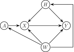
We simulate $M=1000$ datasets each for a range of sample sizes $N$. The nuisance parameters $\operatorname{\mathbb{E}}[A|W]$, $\operatorname{\mathbb{E}}[X|W]$, and $\operatorname{\mathbb{E}}[Y|W]$ are estimated with additive cubic B-splines with $\big{\lceil}N^{\frac{1}{5}}\big{\rceil}+2$ degrees of freedom. The simulation results are displayed in Figure 2. This figure displays the coverage, power, and relative length of the $95\%$ confidence intervals for $\beta_{0}$ using “standard” DML (red) and the newly proposed methods regDML (blue) and regsDML (green). The regDML method is a version of regsDML with regularization only but no selection. If the blue curve is not visible in Figure 2, it coincides with the green curve. The dashed lines in the coverage and power plots indicate $95\%$ confidence regions with respect to uncertainties in the $M$ simulation runs.

The regsDML method succeeds in producing much narrower confidence intervals than DML although it maintains good coverage. The power of regsDML is close to $1$ for all considered sample sizes. For small sample sizes, regsDML leads to confidence intervals whose length is around $10\%-20\%$ the length of DML’s. As the sample size increases, regsDML starts to resemble the behavior of the DML estimator but continues to produce substantially shorter confidence intervals. Thus, the regularization-selection regsDML (and also its version with regularization only) is a highly effective method to increase the power and sharpness of statistical inference whereas keeping the type I error and coverage under control.

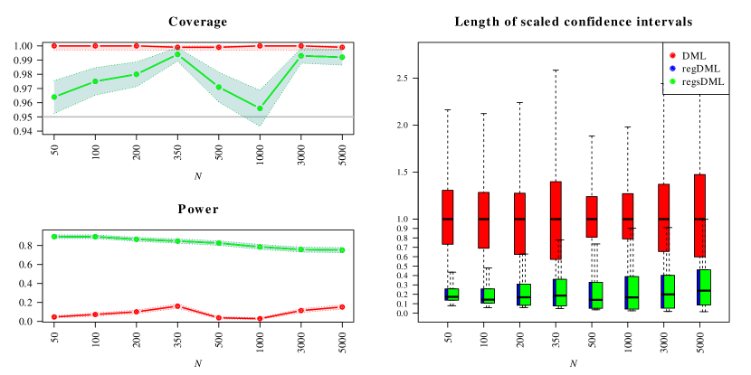
Figure 2: The results come from $M=1000$ simulation runs each from the SEM in Figure 1 for a range of sample sizes $N$ and with $K=2$ and $\mathcal{S}=100$ in Algorithm 1. The nuisance functions are estimated with additive splines. The figure displays the coverage of two-sided confidence intervals for $\beta_{0}$, power for two-sided testing of the hypothesis $H_{0}:\ \beta_{0}=0$, and scaled lengths of two-sided confidence intervals of DML (red), regDML (blue), and regsDML  (green), where all results are at level $95\%$. At each $N$, the lengths of the confidence intervals are scaled with the median length from DML. The shaded regions in the coverage and power plots represent $95\%$ confidence bands with respect to the $M$ simulation runs. The blue and green lines are indistinguishable in the left panel.

Simulation results with $\beta_{0}=0$ in the SEM of Figure 2 are presented in Figure 7 in Section D in the appendix. Further numerical results are given in Section 5.

1.2 Additional Literature

PLMs have received considerable interest. Härdle et al. (2000) present an overview of estimation methods in purely exogenous PLMs, and many references are given there. The remaining part of this paragraph refers to literature investigating endogenous PLMs. Ai and Chen (2003) consider semiparametric estimation with a sieve estimator. Ma and Carroll (2006) introduce a parametric model for the latent variable. Yao (2012) considers a heteroskedastic error term and a partialling-out scheme (Robinson, 1988; Speckman, 1988). Florens et al. (2012) propose to solve an ill-posed integral equation. Su and Zhang (2016) investigate a partially linear dynamic panel data model with fixed effects and lagged variables and consider sieve IV estimators as well as an approach with solving integral equations. Horowitz (2011) compares inference and other properties of nonparametric and parametric estimation if instruments are employed.

Combining Neyman orthogonality and sample splitting (with cross-fitting) allows a diverse range of estimators and machine learning algorithms to be used to estimate nuisance parameters. This procedure has alternatively been considered in Newey and McFadden (1994), van der Laan and Robins (2003), and Chernozhukov et al. (2018). DML methods have been applied in various situations. Chen et al. (2021) consider instrumental variables quantile regression. Liu et al. (2021) apply DML in logistic partially linear models. Colangelo and Lee (2020) employ doubly debiased machine learning methods to a fully nonparametric equation of the response with a continuous treatment. Knaus (2020) presents an overview of DML methods in unconfounded models. Farbmacher et al. (2020) decompose the causal effect of a binary treatment by a mediation analysis and estimate it by DML. Lewis and Syrgkanis (2020) extend DML to estimate dynamic effects of treatments. Chiang et al. (2021) apply DML under multiway clustered sampling environments. Cui and Tchetgen Tchetgen (2020) propose a technique to reduce the bias of DML estimators.

Nonparametric components can be estimated without sample splitting and cross-fitting if the underlying function class satisfies some entropy conditions; see for instance Mammen and van de Geer (1997). Alternatively, Chen et al. (2016) partial out the nonparametric component using a kernel method and employ the generalized method of moments principle (Hansen, 1982). The mentioned entropy regularity conditions limit the complexity of the function class, and ML algorithms do usually not satisfy them. Particularly, these conditions fail to hold if the dimension of the nonparametric variables increases with the sample size (Chernozhukov et al., 2018).

Double robustness and orthogonality arguments have also been considered in the following works. Okui et al. (2012) consider doubly robust estimation of the parametric part. Their estimator is consistent if either the model for the effect of the measured confounders on the outcome or the model of the effect of the measured confounders on the instrument is correctly specified. Smucler et al. (2019) consider doubly robust estimation of scalar parameters where the nuisance functions are $\ell_{1}$-constrained. Targeted minimum loss based estimators and G-estimators also feature an orthogonality property; an overview is given in DiazOrdaz et al. (2019).

The literature presented in this subsection is related to but rather distinct from our work with the only exception of Chernozhukov et al. (2018). The difference to this latter contribution is highlighted in Section 2 and Section A in the appendix.

Outline of the Paper. Sections 2 and 3 describe the DML estimator. The former section introduces an identifiability condition, and the latter investigates asymptotic properties. Section 4 introduces the regularized regularization-selection estimator regDML and its regularization-only version regDML and investigates their asymptotic properties. Section 5 presents numerical experiments and an empirical real data example. Section 6 concludes our work. Proofs and additional definitions and material are given in the appendix.

Notation. We denote by $[N]$ the set $\{1,2,\ldots,N\}$. We add the probability law as a subscript to the probability operator $\operatorname{\mathbb{P}}$ and the expectation operator $\operatorname{\mathbb{E}}$ whenever we want to emphasize the corresponding dependence. We denote the $L^{p}(P)$ norm by $\lVert\cdot\rVert_{P,p}$ and the Euclidean or operator norm by $\lVert\cdot\rVert$, depending on the context. We implicitly assume that given expectations and conditional expectations exist. We denote by $\stackrel{{\scriptstyle d}}{{\rightarrow}}$ convergence in distribution. Furthermore, we denote by $\mathds{1}_{d\times d}\in\mathbb{R}^{d\times d}$ the $d\times d$ identity matrix and write $\mathds{1}$ if we do not want to underline its dimension.

2 An Identifiability Condition and the DML Estimator

Before we introduce regsDML in Section 4, we present our TSLS-type DML estimator of $\beta_{0}$ because we require it to formulate regsDML. The DML estimator estimates the linear coefficient in an endogenous and potentially overidentified PLM where $A$ and $X$ may me multidimensional. Our work builds on Chernozhukov et al. (2018), but they only consider univariate $A$ and $X$ and restrict conditional moments to identify the linear coefficient. We impose an unconditional moment restriction below. However, our results recover theirs if $A$ and $X$ are univariate and the additional conditional moment restrictions are satisfied.

Our PLM is cast as an SEM. The SEM specifies the generating mechanism of the random variables $A$, $W$, $H$, $X$, and $Y$ of dimensions $q$, $v$, $r$, $d$, and $1$, respectively. The structural equation of the response is given by

$$Y\leftarrow X^{T}\beta_{0}+g_{Y}(W)+h_{Y}(H)+\varepsilon_{Y}$$ (3)

as in (1), where $\beta_{0}\in\mathbb{R}^{d}$ is a fixed unknown parameter vector, and where the functions $g_{Y}$ and $h_{Y}$ are unknown. The variable $H$ is hidden and causes endogeneity. The variable $\varepsilon_{Y}$ denotes an unobserved error term. The model is potentially overidentified in the sense that the dimension of $A$ may exceed the dimension of $X$. Observe that $A$ does not directly affect the response $Y$ in the sense that it does not appear on the right hand side of (3). The model is required to satisfy an indentifiability condition as in (5) below.

Econometric models are often presented as a system of simultaneous structural equations. Full information models consider all equations at once, and limited information models only consider equations of interest (Anderson, 1983).

2.1 Identifiability Condition

An identifiability condition is required to identify $\beta_{0}$ in (3). We define the residual terms

$$R_{A}:=A-\operatorname{\mathbb{E}}[A|W],\quad R_{X}:=X-\operatorname{\mathbb{E}}[X|W],\quad\textrm{and}\quad R_{Y}:=Y-\operatorname{\mathbb{E}}[Y|W]$$ (4)

that adjust $A$, $X$, and $Y$ for $W$. Our DML estimator of $\beta_{0}$ is obtained by performing TSLS of $R_{Y}$ on $R_{X}$ using the instrument $R_{A}$. This scheme requires the unconditional moment condition

$$\operatorname{\mathbb{E}}\big{[}R_{A}(R_{Y}-R_{X}^{T}\beta_{0})\big{]}=\boldsymbol{0}$$ (5)

to identify $\beta_{0}$ in (3). For instance, this condition is satisfied if $A$ is independent of both $H$ and $\varepsilon_{Y}$ given $W$ or if $A$ is independent of $H$, $\varepsilon_{Y}$, and $W$. The identifiability condition (5) is strictly weaker than the conditional moment conditions introduced in Chernozhukov et al. (2018); see Section A in the appendix that presents an example where our identifiability condition holds but the conditional moment conditions do not. The subsequent theorem asserts identifiability of $\beta_{0}$.

Theorem 2.1.

Let the dimensions $q=\mathrm{dim}(A)$ and $d=\mathrm{dim}(X)$, and assume $q\geq d$. Assume furthermore that the matrices $\operatorname{\mathbb{E}}[R_{X}R_{A}^{T}]$ and $\operatorname{\mathbb{E}}[R_{A}R_{A}^{T}]$ are of full rank, and assume the identifiability condition (5). We then have

$$\beta_{0}=\Big{(}\operatorname{\mathbb{E}}\big{[}R_{X}R_{A}^{T}\big{]}\operatorname{\mathbb{E}}\big{[}R_{A}R_{A}^{T}\big{]}^{-1}\operatorname{\mathbb{E}}\big{[}R_{A}R_{X}^{T}\big{]}\Big{)}^{-1}\operatorname{\mathbb{E}}\big{[}R_{X}R_{A}^{T}\big{]}\operatorname{\mathbb{E}}\big{[}R_{A}R_{A}^{T}\big{]}^{-1}\operatorname{\mathbb{E}}[R_{A}R_{Y}].$$

Theorem 2.1 precludes underidentification. The full rank condition of the matrix $\operatorname{\mathbb{E}}_{P}[R_{X}R_{A}^{T}]$ expresses that the correlation between $X$ and $A$ is strong enough after regressing out $W$. This is a typical TSLS assumption (Theil, 1953a, b; Basmann, 1957; Bowden and Turkington, 1985; Angrist et al., 1996; Anderson, 2005). The rank assumptions in Theorem 2.1 in particular require that $A$, $X$, and $Y$ are not deterministic functions of $W$.

The instrument $A$ instead of $R_{A}$ can alternatively identify $\beta_{0}$ in Theorem 2.1. However, this procedure leads to a suboptimal convergence rate of the resulting estimator; see Section 3.1.

The identifiability condition (5) is central to Theorem 2.1. Section G in the appendix presents examples illustrating SEMs where the identifiability condition holds and where it fails to hold.

2.2 Alternative Interpretations of $\beta_{0}$

We present two alternative interpretations of $\beta_{0}$ apart from performing TSLS of $R_{Y}$ on $R_{X}$ using the instrument $R_{A}$. The second representation will be used to formulate our regularization schemes in Section 4. To formulate these alternative representations, we introduce the linear projection operator $P_{R_{A}}$ on $R_{A}$ that maps a random variable $Z$ to its projection

$$P_{R_{A}}Z:=\operatorname{\mathbb{E}}\big{[}ZR_{A}^{T}\big{]}\operatorname{\mathbb{E}}\big{[}R_{A}R_{A}^{T}\big{]}^{-1}R_{A}.$$

By Theorem 2.1, the population parameter $\beta_{0}$ solves the TSLS moment equation

$$\boldsymbol{0}=\operatorname{\mathbb{E}}\big{[}R_{X}R_{A}^{T}\big{]}\operatorname{\mathbb{E}}\big{[}R_{A}R_{A}^{T}\big{]}^{-1}\operatorname{\mathbb{E}}\big{[}R_{A}(R_{Y}-R_{X}^{T}\beta_{0})\big{]}.$$

This motivates a generalized method of moments interpretation of $\beta_{0}$ because we have

$$\beta_{0}=\operatorname*{arg\,min}_{\beta\in\mathbb{R}^{d}}\operatorname{\mathbb{E}}[\psi(S;\beta,\eta^{0})]\operatorname{\mathbb{E}}\big{[}R_{A}R_{A}^{T}\big{]}^{-1}\operatorname{\mathbb{E}}\big{[}\psi^{T}(S;\beta,\eta^{0})\big{]}$$

for $\psi(S;\beta,\eta^{0})=R_{A}(R_{Y}-R_{X}^{T}\beta)$, where $\eta^{0}=(\operatorname{\mathbb{E}}[A|W],\operatorname{\mathbb{E}}[X|W],\operatorname{\mathbb{E}}[Y|W])$ denotes the nuisance parameter and $S=(A,W,X,Y)$ denotes the concatenation of the observable variables.

This leads to the second interpretation of $\beta_{0}$. The coefficient $\beta_{0}$ minimizes the squared projection of the residual $R_{Y}-R_{X}^{T}\beta$ on $R_{A}$, namely

$$\beta_{0}=\operatorname*{arg\,min}_{\beta\in\mathbb{R}^{d}}\operatorname{\mathbb{E}}\Big{[}\big{(}P_{R_{A}}(R_{Y}-R_{X}^{T}\beta)\big{)}^{2}\Big{]}.$$ (6)

We employ the representation of $\beta_{0}$ in (6) to formulate our regularization schemes in Section 4.

3 Formulation of the DML Estimator and its Asymptotic Properties

In this section, we describe how to estimate $\beta_{0}$ using the TSLS-type DML scheme, and we describe the asymptotic properties of this estimator.

Consider $N$ iid realizations $\{S_{i}=(A_{i},X_{i},W_{i},Y_{i})\}_{i\in[N]}$ of $S=(A,X,W,Y)$ from the SEM in (3). We concatenate the observations of $A$ row-wise to form an $(N\times q)$-dimensional matrix $\boldsymbol{A}$. Analogously, we construct the matrices $\boldsymbol{X}\in\mathbb{R}^{N\times d}$ and $\boldsymbol{W}\in\mathbb{R}^{N\times v}$ and the vector $\boldsymbol{Y}\in\mathbb{R}^{N}$ containing the respective observations.

We construct a DML estimator of $\beta_{0}$ as follows. First, we split the data into $K\geq 2$ disjoint sets $I_{1},\ldots,I_{K}$. For simplicity, we assume that these sets are of equal cardinality $n=\frac{N}{K}$. In practice, their cardinality might differ due to rounding issues.

For each $k\in[K]$, we estimate the conditional expectations $m_{A}^{0}(W):=\operatorname{\mathbb{E}}[A|W]$, $m_{X}^{0}(W):=\operatorname{\mathbb{E}}[X|W]$, and $m_{Y}^{0}(W):=\operatorname{\mathbb{E}}[Y|W]$, which act as nuisance parameters, with data from $I_{k}^{c}$. We call the resulting estimators $\hat{m}_{A}^{I_{k}^{c}}$, $\hat{m}_{X}^{I_{k}^{c}}$, and $\hat{m}_{Y}^{I_{k}^{c}}$, respectively. Then, the adjusted residual terms $\widehat{R}_{A,i}^{I_{k}}:=A_{i}-\hat{m}_{A}^{I_{k}^{c}}(W_{i})$, $\widehat{R}_{X,i}^{I_{k}}:=X_{i}-\hat{m}_{X}^{I_{k}^{c}}(W_{i})$, and $\widehat{R}_{Y,i}^{I_{k}}:=Y_{i}-\hat{m}_{Y}^{I_{k}^{c}}(W_{i})$ for $i\in I_{k}$ are evaluated on $I_{k}$, the complement of $I_{k}^{c}$. We concatenate them row-wise to form the matrices $\widehat{\boldsymbol{R}}^{I_{k}}_{\boldsymbol{A}}\in\mathbb{R}^{n\times q}$ and $\widehat{\boldsymbol{R}}^{I_{k}}_{\boldsymbol{X}}\in\mathbb{R}^{n\times d}$ and the vector $\widehat{\boldsymbol{R}}^{I_{k}}_{\boldsymbol{Y}}\in\mathbb{R}^{n}$.

These $K$ iterates are assembled to form the DML estimator

$$\hat{\beta}:=\bigg{(}\frac{1}{K}\sum_{k=1}^{K}\big{(}\widehat{\boldsymbol{R}}^{I_{k}}_{\boldsymbol{X}}\big{)}^{T}\Pi_{\widehat{\boldsymbol{R}}^{I_{k}}_{\boldsymbol{A}}}\widehat{\boldsymbol{R}}^{I_{k}}_{\boldsymbol{X}}\bigg{)}^{-1}\frac{1}{K}\sum_{k=1}^{K}\big{(}\widehat{\boldsymbol{R}}^{I_{k}}_{\boldsymbol{X}}\big{)}^{T}\Pi_{\widehat{\boldsymbol{R}}^{I_{k}}_{\boldsymbol{A}}}\widehat{\boldsymbol{R}}^{I_{k}}_{\boldsymbol{Y}}$$ (7)

of $\beta_{0}$, where

$$\Pi_{\widehat{\boldsymbol{R}}^{I_{k}}_{\boldsymbol{A}}}:=\widehat{\boldsymbol{R}}^{I_{k}}_{\boldsymbol{A}}\Big{(}\big{(}\widehat{\boldsymbol{R}}^{I_{k}}_{\boldsymbol{A}}\big{)}^{T}\widehat{\boldsymbol{R}}^{I_{k}}_{\boldsymbol{A}}\Big{)}^{-1}\big{(}\widehat{\boldsymbol{R}}^{I_{k}}_{\boldsymbol{A}}\big{)}^{T}$$ (8)

denotes the orthogonal projection matrix onto the space spanned by the columns of $\widehat{\boldsymbol{R}}^{I_{k}}_{\boldsymbol{A}}$.

To obtain $\hat{\beta}$ in (7), the individual matrices are first averaged before the final matrix is inverted. It is also possible to compute $K$ individual TSLS estimators on the $K$ iterates individually and average these. Both schemes are asymptotically equivalent. Chernozhukov et al. (2018) call these two schemes DML2 and DML1, respectively, where DML2 is as in (7). The DML1 version of the coefficient estimator is given in the appendix in Section B.1. The advantage of DML2 over DML1 is that it enhances stability properties of the estimator. To ensure stability of the DML1 estimator, every individual matrix that is inverted needs to be well conditioned. Stability of the DML2 estimator is ensured if the average of these matrices is well conditioned.

The $K$ sample splits are random. To reduce the effect of this randomness, we repeat the overall procedure $\mathcal{S}$ times and assemble the results as suggested in Chernozhukov et al. (2018). This procedure is described in Algorithm 1 in Section 4.2 below.

The following theorem establishes that $\hat{\beta}$ converges at the parametric rate and is asymptotically Gaussian.

Theorem 3.1.

Consider model (3). Suppose that Assumption I.5 in the appendix in Section I holds and consider $\overline{\psi}$ given in Definition I.1 in the appendix in Section I. Then $\hat{\beta}$ as in (7) concentrates in a $\frac{1}{\sqrt{N}}$ neighborhood of $\beta_{0}$. It is approximately linear and centered Gaussian, namely

$$\sqrt{N}\sigma^{-1}(\hat{\beta}-\beta_{0})=\frac{1}{\sqrt{N}}\sum_{i=1}^{N}\overline{\psi}(S_{i};\beta_{0},\eta^{0})+o_{P}(1)\stackrel{{\scriptstyle d}}{{\rightarrow}}\mathcal{N}(0,\mathds{1}_{d\times d})\quad(N\rightarrow\infty),$$

uniformly over the law $P$ of $S=(A,W,X,Y)$, and where the variance-covariance matrix $\sigma^{2}$ is given by $\sigma^{2}=J_{0}\tilde{J}_{0}J_{0}^{T}$ for the matrices $\tilde{J}_{0}$ and $J_{0}$ given in Definition I.1 in the appendix.

A similar result to Theorem 3.1 is presented by Chernozhukov et al. (2018). However, their result requires univariate $A$ and $X$, and it imposes conditional moment restrictions instead of the identifiability condition (5); see also Section A in the appendix that presents an example where our identifiability condition holds but the conditional moment conditions do not. If $A$ and $X$ are univariate and the respective conditional moment conditions hold, our result coincides with Chernozhukov et al. (2018).

Theorem 3.1 also holds for the DML1 version of $\hat{\beta}$ defined in the appendix in Section B.1. Assumption I.5 specifies regularity conditions and the convergence rate of the machine learners estimating the conditional expectations. The machine learners are required to satisfy the product relations

$$\begin{array}[]{l}\lVert m_{A}^{0}(W)-\hat{m}_{A}^{I_{k}^{c}}(W)\rVert_{P,2}^{2}\ll N^{-\frac{1}{2}},\\ \lVert m_{A}^{0}(W)-\hat{m}_{A}^{I_{k}^{c}}(W)\rVert_{P,2}\big{(}\lVert m_{Y}^{0}(W)-\hat{m}_{Y}^{I_{k}^{c}}(W)\rVert_{P,2}+\lVert m_{X}^{0}(W)-\hat{m}_{X}^{I_{k}^{c}}(W)\rVert_{P,2}\big{)}\ll N^{-\frac{1}{2}}\end{array}$$ (9)

for $k\in[K]$, which allows us to employ a broad range of ML estimators. For instance, these convergence rates are satisfied by $\ell_{1}$-penalized and related methods in a variety of sparse, high-dimensional linear models (Candes and Tao, 2007; Bickel et al., 2009; Bühlmann and van de Geer, 2011; Belloni and Chernozhukov, 2013), forward selection in sparse linear models (Kozbur, 2020), high-dimensional additive models (Meier et al., 2009; Koltchinskii and Yuan, 2010; Yuan and Zhou, 2016), or regression trees and random forests (Wager and Walther, 2016; Athey et al., 2019). Please see Chernozhukov et al. (2018) for additional references. In particular, the rate condition (9) is satisfied if the individual ML estimators converge at rate $N^{-\frac{1}{4}}$. Therefore, the individual ML estimators are not required to converge at rate $N^{-\frac{1}{2}}$.

The asymptotic variance $\sigma^{2}$ can be consistently estimated by replacing the true $\beta_{0}$ by $\hat{\beta}$ or its DML1 version. The nuisance functions are estimated on subsampled datasets, and the estimator of $\sigma^{2}$ is obtained by cross-fitting. The formal definition, the consistency result, and its proof are given in Definition I.1 and in Theorem I.21 in the appendix in Section I.

For fixed $P$, the asymptotic variance-covariance matrix $\sigma^{2}$ is the same as if the conditional expectations $m_{A}^{0}(W)$, $m_{X}^{0}(W)$, and $m_{Y}^{0}(W)$ and hence $R_{A}$, $R_{X}$, and $R_{Y}$ were known.

Theorem 3.1 holds uniformly over laws $P$. This uniformity guarantees some robustness of the asymptotic statement (Chernozhukov et al., 2018). The dimension $v$ of the covariate $W$ may grow as the sample size increases. Thus, high-dimensional methods can be considered to estimate the conditional expectations $\operatorname{\mathbb{E}}[A|W]$, $\operatorname{\mathbb{E}}[X|W]$, and $\operatorname{\mathbb{E}}[Y|W]$.

The estimator $\hat{\beta}$ solves the moment equations

$$\boldsymbol{0}=\frac{1}{K}\sum_{k=1}^{K}\bigg{(}\frac{1}{n}\sum_{i\in I_{k}}\widehat{R}_{X,i}^{I_{k}}\big{(}\widehat{R}_{A,i}^{I_{k}}\big{)}^{T}\Big{(}\frac{1}{n}\sum_{i\in I_{k}}\widehat{R}_{A,i}^{I_{k}}\big{(}\widehat{R}_{A,i}^{I_{k}}\big{)}^{T}\Big{)}^{-1}\frac{1}{n}\sum_{i\in I_{k}}\psi(S_{i};\hat{\beta},\hat{\eta}^{I_{k}^{c}})\bigg{)},$$

where the score function $\psi$ is given by

$$\psi(S;\beta,\eta):=\big{(}A-m_{A}(W)\big{)}\Big{(}Y-m_{Y}(W)-\big{(}X-m_{X}(W)\big{)}^{T}\beta\Big{)}$$ (10)

for $\eta=(m_{A},m_{X},m_{Y})$, and where the estimated nuisance parameter is given by $\hat{\eta}^{I_{k}^{c}}=(\hat{m}_{A}^{I_{k}^{c}},\hat{m}_{X}^{I_{k}^{c}},\hat{m}_{Y}^{I_{k}^{c}})$. Observe that $\psi(S;\beta_{0},\eta^{0})$ with $\eta^{0}=(m_{A}^{0},m_{X}^{0},m_{Y}^{0})$ coincides with the term whose expectation is constrained to equal $\boldsymbol{0}$ in the identifiability condition (5). The crucial step to prove asymptotic normality of $\sqrt{N}(\hat{\beta}-\beta_{0})$ is to analyze the asymptotic behavior of $\frac{1}{\sqrt{n}}\sum_{i\in I_{k}}\psi(S_{i};\hat{\beta},\hat{\eta}^{I_{k}^{c}})$ for $k\in[K]$.

Apart from the identifiability condition, the first fundamental requirement to analyze these terms is the ML convergence rates in (9). Second, we employ sample splitting and cross-fitting. Sample splitting ensures that the data used to estimate the nuisance parameters and the data on which these estimators are evaluated are independent. Cross-fitting enables us to regain full efficiency. The third requirement is that the underlying score function $\psi$ in (10) is Neyman orthogonal, which we explain next.

Neyman orthogonality ensures that $\psi$ is insensitive to small changes in the nuisance parameter $\eta$ at the true unknown linear coefficient $\beta_{0}$ and the true unknown nuisance parameter $\eta^{0}$. This makes estimation of $\beta_{0}$ robust to inserting biased ML estimators of the nuisance parameter in the estimation equation. The following definition formally introduces this concept.

Definition 3.2.

(Chernozhukov et al., 2018, Definition 2.1). A score $\psi=\psi(S;\beta,\eta)$ is Neyman orthogonal at $(\beta_{0},\eta^{0})$ if the pathwise derivative map

$$\frac{\partial}{\partial r}\operatorname{\mathbb{E}}_{P}\big{[}\psi\big{(}S;\beta_{0},\eta^{0}+r(\eta-\eta^{0})\big{)}\big{]}$$

exists for all $r\in[0,1)$ and nuisance parameters $\eta$ and vanishes at $r=0$.

Definition 3.2 does not entirely coincide with Chernozhukov et al. (2018, Definition 2.1) because the latter also includes an identifiability condition. We directly assume the identifiability condition (5).

The subsequent proposition states that the score function $\psi$ in (10) is indeed Neyman orthogonal.

Proposition 3.3.

The score $\psi$ given in Equation (10) is Neyman orthogonal.

We would like to remark that Neyman orthogonality of $\psi$ neither depends on the distribution of $S$ nor on the value of the coefficients $\beta_{0}$ and $\eta^{0}$. In addition to being Neyman orthogonal, $\psi$ is linear in $\beta$ in the sense that we have

$$\psi(S;\beta,\eta)=\psi^{b}(S;\eta)-\psi^{a}(S;\eta)\beta$$ (11)

for

$$\psi^{b}(S;\eta):=\big{(}A-m_{A}(W)\big{)}\big{(}Y-m_{Y}(W)\big{)}$$

and

$$\psi^{a}(S;\eta):=\big{(}A-m_{A}(W)\big{)}\big{(}X-m_{X}(W)\big{)}^{T}.$$

This linearity property is also employed in the proof of Theorem 3.1.

3.1 Suboptimal Estimation Procedure

In general, we cannot employ $A$ as an instrument instead of $R_{A}$ in our TSLS-type DML estimation procedure. For simplicity, we assume $K=2$ in this subsection and consider disjoint index sets $I$ and $I^{c}$ of size $n=\frac{N}{2}$. The term

$$\frac{1}{\sqrt{n}}\sum_{i\in I}A_{i}\big{(}\widehat{R}_{Y,i}^{I}-(\widehat{R}_{X,i}^{I})^{T}\beta_{0}\big{)}$$ (12)

can diverge as $N\rightarrow\infty$ because $\hat{m}_{X}^{I^{c}}$ and $\hat{m}_{Y}^{I^{c}}$ can be biased estimators of $m_{X}^{0}$ and $m_{Y}^{0}$. This in particular happens if the functions $m_{X}^{0}$ and $m_{Y}^{0}$ are high-dimensional and need to be estimated by regularization techniques; see Chernozhukov et al. (2018). Even if sample splitting is employed, the term (12) is asymptotically not well behaved because the underlying score function

$$\varphi(S;\beta,\eta):=A\Big{(}Y-m_{Y}(W)-\big{(}X-m_{X}(W)\big{)}^{T}\beta\Big{)}$$

is not Neyman orthogonal. The issue is illustrated in Figure 3. The SEM used to generate the data is similar to the nonconfounded model used in Chernozhukov et al. (2018, Figure 1). The centered and rescaled term $\frac{\hat{\beta}-\beta_{0}}{\widehat{\operatorname{\textrm{Var}}}(\hat{\beta})}$ using $A$ as an instrument is biased whereas it is not if the instrument $R_{A}$ is used. Here, $\widehat{\operatorname{\textrm{Var}}}(\hat{\beta})$ denotes the empirically observed variance of $\hat{\beta}$ with respect to the performed simulation runs.

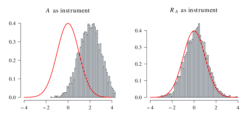
Figure 3: Histograms of $\frac{\hat{\beta}-\beta_{0}}{\widehat{\operatorname{\textrm{Var}}}(\hat{\beta})}$, where $\widehat{\operatorname{\textrm{Var}}}(\hat{\beta})$ denotes the empirically observed variance of $\hat{\beta}$ with respect to the simulation runs, using $A$ as an instrument in the left plot and using $R_{A}$ as an instrument in the right plot. The orange curves represent the density of $\mathcal{N}(0,1)$. The results come from $5000$ simulation runs of sample size $5000$ each from the SEM in the appendix in Section C with $K=2$. The conditional expectations are estimated with random forests consisting of $500$ trees that have a minimal node size of $5$.

4 Regularizing the DML Estimator: regDML and regsDML

We introduce a regularized estimator, regsDML, whose estimated standard deviation is typically smaller and never worse than the one of the TSLS-type DML estimator described above. Supporting theory and simulations illustrate that the associated confidence intervals nevertheless reach valid andgood coverage. The regsDML estimator selects either the DML estimator or its regularization-only version regDML, depending on which of the two estimators has a smaller estimated standard deviation.

Subsequently, we first introduce the regularization-only method regDML. The regDML estimator is obtained by regularizing DML and choosing a data-dependent regularization parameter. Before we describe the choice of the regularization parameter, we introduce the regularization scheme for fixed regularization parameters.

Given a regularization parameter $\gamma\geq 0$, the population coefficient $b^{\gamma}$ of the regularization scheme optimizes an objective function similar to the one used in k-class regression (Theil, 1961) or anchor regression (Rothenhäusler et al., 2021; Bühlmann, 2020). We established the representation

$$\beta_{0}=\operatorname*{arg\,min}_{\beta\in\mathbb{R}^{d}}\operatorname{\mathbb{E}}\Big{[}\big{(}P_{R_{A}}(R_{Y}-R_{X}^{T}\beta)\big{)}^{2}\Big{]}$$

of $\beta_{0}$ in (6). For a regularization parameter $\gamma\geq 0$, we consider the regularized objective function and corresponding population coefficient

$$b^{\gamma}:=\operatorname*{arg\,min}_{\beta\in\mathbb{R}^{d}}\operatorname{\mathbb{E}}\Big{[}\big{(}(\operatorname{\mathrm{Id}}-P_{R_{A}})(R_{Y}-R_{X}^{T}\beta)\big{)}^{2}\Big{]}+\gamma\operatorname{\mathbb{E}}\Big{[}\big{(}P_{R_{A}}(R_{Y}-R_{X}^{T}\beta)\big{)}^{2}\Big{]}.$$ (13)

This regularized objective is form-wise analogous to the objective function employed in anchor regression. The anchor regression estimator has been reformulated as a k-class estimator by Jakobsen and Peters (2020) for a linear model.

If $\gamma=1$, ordinary least squares regression of $R_{Y}$ on $R_{X}$ is performed. If $\gamma=0$, we are partialling out or adjusting for the variable $R_{A}$. If $\gamma=\infty$, we perform TSLS regression of $R_{Y}$ on $R_{X}$ using the instrument $R_{A}$. In this case, $b^{\gamma}$ coincides with $\beta_{0}$. The coefficient $b^{\gamma}$ interpolates between the OLS coefficient $b^{\gamma=1}$ and the TSLS coefficient $\beta_{0}$ for general choices of $\gamma>1$. For $\gamma>1$, there is a one to one correspondence between $b^{\gamma}$ and the k-class estimator (based on $R_{A}$, $R_{X}$, and $R_{Y}$) with regularization parameter $\kappa=\frac{\gamma-1}{\gamma}\in(0,1)$; see Jakobsen and Peters (2020).

4.1 Estimation and Asymptotic Normality

In this section, we describe how to estimate $b^{\gamma}$ in (13) for fixed $\gamma\geq 0$ using a DML scheme, and we describe the asymptotic properties of this estimator. We consider the residual matrices $\widehat{\boldsymbol{R}}^{I_{k}}_{\boldsymbol{A}}\in\mathbb{R}^{n\times q}$ and $\widehat{\boldsymbol{R}}^{I_{k}}_{\boldsymbol{X}}\in\mathbb{R}^{n\times d}$ and the vector $\widehat{\boldsymbol{R}}^{I_{k}}_{\boldsymbol{Y}}\in\mathbb{R}^{n}$ introduced in Section 3 that adjust the data with respect to the nonparametric variables. The estimator of $b^{\gamma}$ is given by

$$\hat{b}^{\gamma}:=\operatorname*{arg\,min}_{b\in\mathbb{R}^{d}}\frac{1}{K}\sum_{k=1}^{K}\bigg{(}\Big{\lVert}\big{(}\mathds{1}-\Pi_{\widehat{\boldsymbol{R}}^{I_{k}}_{\boldsymbol{A}}}\big{)}\big{(}\widehat{\boldsymbol{R}}^{I_{k}}_{\boldsymbol{Y}}-\big{(}\widehat{\boldsymbol{R}}^{I_{k}}_{\boldsymbol{X}}\big{)}^{T}b\big{)}\Big{\rVert}_{2}^{2}+\gamma\Big{\lVert}\Pi_{\widehat{\boldsymbol{R}}^{I_{k}}_{\boldsymbol{A}}}(\widehat{\boldsymbol{R}}^{I_{k}}_{\boldsymbol{Y}}-(\widehat{\boldsymbol{R}}^{I_{k}}_{\boldsymbol{X}})^{T}b)\Big{\rVert}_{2}^{2}\bigg{)},$$

where $\Pi_{\widehat{\boldsymbol{R}}^{I_{k}}_{\boldsymbol{A}}}$ is as in (8). This estimator can be expressed in closed form by

$$\hat{b}^{\gamma}=\bigg{(}\frac{1}{K}\sum_{k=1}^{K}\big{(}\widehat{\boldsymbol{R}}^{I_{k}}_{\widetilde{\boldsymbol{X}}}\big{)}^{T}\widehat{\boldsymbol{R}}^{I_{k}}_{\widetilde{\boldsymbol{X}}}\bigg{)}^{-1}\frac{1}{K}\sum_{k=1}^{K}\big{(}\widehat{\boldsymbol{R}}^{I_{k}}_{\widetilde{\boldsymbol{X}}}\big{)}^{T}\widehat{\boldsymbol{R}}^{I_{k}}_{\widetilde{\boldsymbol{Y}}},$$ (14)

where

$$\widehat{\boldsymbol{R}}^{I_{k}}_{\widetilde{\boldsymbol{X}}}:=\Big{(}\mathds{1}+(\sqrt{\gamma}-1)\Pi_{\widehat{\boldsymbol{R}}^{I_{k}}_{\boldsymbol{A}}}\Big{)}\widehat{\boldsymbol{R}}^{I_{k}}_{\boldsymbol{X}}\quad\textrm{and}\quad\widehat{\boldsymbol{R}}^{I_{k}}_{\widetilde{\boldsymbol{Y}}}:=\Big{(}\mathds{1}+(\sqrt{\gamma}-1)\Pi_{\widehat{\boldsymbol{R}}^{I_{k}}_{\boldsymbol{A}}}\Big{)}\widehat{\boldsymbol{R}}^{I_{k}}_{\boldsymbol{Y}}.$$ (15)

The computation of $\hat{b}^{\gamma}$ is similar to an OLS scheme where $\widehat{\boldsymbol{R}}^{I_{k}}_{\widetilde{\boldsymbol{Y}}}$ is regressed on $\widehat{\boldsymbol{R}}^{I_{k}}_{\widetilde{\boldsymbol{X}}}$. To obtain $\hat{b}^{\gamma}$, individual matrices are first averaged before the final matrix is inverted. It is also possible to directly carry out the $K$ OLS regressions of $\widehat{\boldsymbol{R}}^{I_{k}}_{\widetilde{\boldsymbol{Y}}}$ on $\widehat{\boldsymbol{R}}^{I_{k}}_{\widetilde{\boldsymbol{X}}}$ and average the resulting parameters. Both schemes are asymptotically equivalent. We call the two schemes DML2 and DML1, respectively. This is analogous to Chernozhukov et al. (2018) as already mentioned in Section 3. The DML1 version is presented in the appendix in Section B.2. As mentioned in Section 3, the advantage of DML2 over DML1 is that it enhances stability properties of the coefficient estimator because the average of matrices needs to be well conditioned but not every individual matrix.

Theorem 4.1.

Let $\gamma\geq 0$. Suppose that Assumption I.5 in the appendix in Section I (same as in Theorem 3.1) except I.5.1 holds, and consider the quantities $\sigma^{2}(\gamma)$ and $\overline{\psi}$ introduced in Definition J.1 in the appendix in Section J. The estimator $\hat{b}^{\gamma}$ concentrates in a $\frac{1}{\sqrt{N}}$ neighborhood of $b^{\gamma}$. It is approximately linear and centered Gaussian, namely

$$\sqrt{N}\sigma^{-1}(\gamma)(\hat{b}^{\gamma}-b^{\gamma})=\frac{1}{\sqrt{N}}\sum_{i=1}^{N}\overline{\psi}(S_{i};b^{\gamma},\eta^{0})+o_{P}(1)\stackrel{{\scriptstyle d}}{{\rightarrow}}\mathcal{N}(0,\mathds{1}_{d\times d})\quad(N\rightarrow\infty),$$

uniformly over laws $P$ of $S=(A,W,X,Y)$.

Theorem 4.1 also holds for the DML1 version of $\hat{b}^{\gamma}$ defined in the appendix in Section B.2. The influence function is denoted by $\overline{\psi}$ in both Theorems 3.1 and 4.1 but is defined differently. Assumption I.5 specifies regularity conditions and the convergence rate of the machine learners of the conditional expectations. The machine learners are required to satisfy the product relations

$$\begin{array}[]{l}\lVert m_{A}^{0}(W)-\hat{m}_{A}^{I_{k}^{c}}(W)\rVert_{P,2}^{2}\ll N^{-\frac{1}{2}},\\ \lVert m_{X}^{0}(W)-\hat{m}_{X}^{I_{k}^{c}}(W)\rVert_{P,2}\big{(}\lVert m_{Y}^{0}(W)-\hat{m}_{Y}^{I_{k}^{c}}(W)\rVert_{P,2}+\lVert m_{X}^{0}(W)-\hat{m}_{X}^{I_{k}^{c}}(W)\rVert_{P,2}\big{)}\ll N^{-\frac{1}{2}},\\ \lVert m_{A}^{0}(W)-\hat{m}_{A}^{I_{k}^{c}}(W)\rVert_{P,2}\big{(}\lVert m_{Y}^{0}(W)-\hat{m}_{Y}^{I_{k}^{c}}(W)\rVert_{P,2}+\lVert m_{X}^{0}(W)-\hat{m}_{X}^{I_{k}^{c}}(W)\rVert_{P,2}\big{)}\ll N^{-\frac{1}{2}}\end{array}$$

for $k\in[K]$. The main difference to Theorem 3.1 and quantity of interest is the asymptotic variance $\sigma^{2}(\gamma)$. It can be consistently estimated with either $\hat{b}^{\gamma}$ or its DML1 version as illustrated in Theorem J.3 in the appendix in Section J. Typically, for $\gamma<\infty$, the asymptotic variance $\sigma^{2}(\gamma)$ is smaller than $\sigma^{2}$ in Theorem 3.1. Such a variance gain comes at the price of bias because $\hat{b}^{\gamma}$ estimates $b^{\gamma}$ and not the true parameter $\beta_{0}$.

The proof of Theorem 4.1 uses Neyman orthogonality of the underlying score function. Recall that Neyman orthogonality neither depends on the distribution of $S$ nor on the value of the coefficients $\beta_{0}$ and $\eta^{0}$ as discussed in Section 3.

For fixed $\gamma>1$, Theorem 4.1 furthermore implies that the k-class estimator corresponding to $\hat{b}^{\gamma}$ converges at the parametric rate and follows a Gaussian distribution asymptotically.

4.2 Estimating the Regularization Parameter $\gamma$

For simplicity, we assume $d=1$ in this subsection. The results can be extended to $d>1$.

Subsequently, we introduce a data-driven method to choose the regularization parameter $\gamma$ in practice. This scheme first optimizes the estimated asymptotic MSE of $\hat{b}^{\gamma}$. The estimated regularization for the parameter $\gamma$ leads to an estimate of $\beta_{0}$ that asymptotically has the same MSE behavior as the TSLS-type estimator $\hat{\beta}$ in (7) but may exhibit substantially better finite sample properties.

We consider the estimated regularization parameter

$$\hat{\gamma}:=\operatorname*{arg\,min}_{\gamma\geq 0}\frac{1}{N}\hat{\sigma}^{2}(\gamma)+\lvert\hat{b}^{\gamma}-\hat{\beta}\rvert^{2}.$$ (16)

It optimizes an estimate of the asymptotic MSE of $\hat{b}^{\gamma}$: the term $\hat{\sigma}^{2}(\gamma)$ is the consistent estimator of $\sigma^{2}(\gamma)$ described in Theorem J.3 in the appendix in Section J, and the term $\lvert\hat{b}^{\gamma}-\hat{\beta}\rvert^{2}$ is a plug-in estimator of the squared population bias $\lvert b^{\gamma}-\beta_{0}\rvert^{2}$. The estimated regularization parameter $\hat{\gamma}$ is random because it depends on the data.

First, we investigate the bias of the population parameter $b^{{\gamma}_{N}}$ for a nonrandom sequence of regularization parameters $\{{\gamma}_{N}\}_{N\geq 1}$ as $N\to\infty$. Afterwards, we propose a modified estimator of the regularization parameter whose corresponding parameter estimate is denoted by regDML, and we introduce the regularization-selection estimator regsDML. Finally, we and analyze the asymptotic properties of regDML and regsDML.

Let us consider a deterministic sequence $\{{\gamma}_{N}\}_{N\geq 1}$ of regularization parameters. By Proposition 4.2 below, the (scaled) population bias $\sqrt{N}\lvert b^{{\gamma}_{N}}-\beta_{0}\rvert$ vanishes as $N\rightarrow\infty$ if ${\gamma}_{N}$ is of larger order than $\sqrt{N}$.

Proposition 4.2.

Suppose that I.5.1, I.5.3, and I.5.4 of Assumption I.5 in the appendix in Section I hold (subset of the assumptions in Theorem 3.1). Assume $\{{\gamma}_{N}\}_{N\geq 1}$ is sequence of non-negative real numbers. Then we have

$$\sqrt{N}\lvert b^{{\gamma}_{N}}-\beta_{0}\rvert\rightarrow\begin{cases}0,&\mbox{if }{\gamma}_{N}\gg\sqrt{N}\\ C,&\mbox{if }{\gamma}_{N}\sim\sqrt{N}\\ \infty,&\mbox{if }{\gamma}_{N}\ll\sqrt{N}\end{cases}$$

as $N\rightarrow\infty$ for some non-negative finite real number $C$.

Theorem 4.3 below shows that the estimated regularization parameter $\hat{\gamma}$ is of equal or larger stochastic order than $\sqrt{N}$. If it were not, choosing $\gamma=\infty$ in (16), and hence selecting the TSLS-type estimator $\hat{\beta}$, would lead to a smaller estimated asymptotic MSE.

Theorem 4.3.

Let ${\gamma}_{N}=o(\sqrt{N})$, and suppose that Assumption I.5 in the appendix in Section I holds (same as in Theorem 3.1). We then have

$$\lim_{N\rightarrow\infty}P\big{(}\hat{\sigma}^{2}({\gamma}_{N})+N(\hat{b}^{{\gamma}_{N}}-\hat{\beta})^{2}\leq\hat{\sigma}^{2}\big{)}=0.$$

If $\hat{\gamma}$ is multiplied by a deterministic scalar $a_{N}$ that diverges to $+\infty$ at an arbitrarily slow rate as $N\rightarrow\infty$, the modified regularization parameter $\hat{\gamma}^{\prime}:=a_{N}\hat{\gamma}$ is of stochastic order larger than $\sqrt{N}$. By default, we choose $a_{N}=\log(\sqrt{N})$. Proposition 4.2 is formulated for deterministic regularization parameters, but the deterministic statements can be replaced by probabilistic ones. Proposition 4.2 then implies that the population bias term $\lvert b^{\hat{\gamma}^{\prime}}-\beta_{0}\rvert$ vanishes at rate $o_{P}(N^{-\frac{1}{2}})$. Thus, the two quantities $\sqrt{N}(\hat{b}^{\hat{\gamma}^{\prime}}-b^{\hat{\gamma}^{\prime}})$ and $\sqrt{N}(\hat{b}^{\hat{\gamma}^{\prime}}-\beta_{0})$ are asymptotically equivalent due to Theorem 4.4 below, and we have

$$\sqrt{N}(\hat{b}^{\hat{\gamma}^{\prime}}-\beta_{0})\approx{\cal N}\big{(}0,\sigma^{2}(\hat{\gamma}^{\prime})\big{)}$$

whenever $N$ is sufficiently large (note that asymptotically as $N\to\infty$, the right-hand side has the same limit as described in Theorem 4.4).

We call $\hat{b}^{\hat{\gamma}^{\prime}}$ the regDML (regularized DML) estimator. The regularization-selection estimator $\hat{b}^{\hat{\gamma}^{\prime}}$ selects between DML and regDML based on whose variance estimate is smaller. The “s” in regsDML stands for selection.

Theorem 4.4.

Suppose that Assumption I.5 in the appendix in Section I holds (same as in Theorem 3.1). Let $\{a_{j}\}_{j\geq 1}$ be a sequence of deterministic, non-negative real numbers that diverges to $\infty$ as $N\rightarrow\infty$. Furthermore, consider $\hat{\gamma}^{\prime}=a_{N}\hat{\gamma}$ as above. Then, we have

$$\sqrt{N}\hat{\sigma}^{-1}(\hat{\gamma}^{\prime})(\hat{b}^{\hat{\gamma}^{\prime}}-b^{\hat{\gamma}^{\prime}})=\sqrt{N}\sigma^{-1}(\hat{\beta}-\beta_{0})+o_{P}(1)$$

uniformly over laws $P$ of $S=(A,W,X,Y)$, where $\hat{\sigma}(\cdot)$ ist the estimator from Theorem J.3 in the appendix, which consistently estimates $\sigma(\cdot)$ from 4.1.

Particularly, $\hat{b}^{\hat{\gamma}^{\prime}}$ and $\hat{\beta}$ are asymptotically equivalent. But $\hat{b}^{\hat{\gamma}^{\prime}}$ may exhibit substantially better finite sample properties as we demonstrate in the subsequent section. Because $\hat{b}^{\hat{\gamma}^{\prime}}$ and $\hat{\beta}$ are asymptotically equivalent, the same result also holds for the selection estimator regsDML.

The proof of Theorem 4.4 does not depend on the precise construction of $\hat{\gamma}^{\prime}$ and only uses that the random regularization parameter is of stochastic order larger than $\sqrt{N}$. Thus, Theorem 4.4 remains valid if the regularization parameter comes from k-class estimaton and is of the required stochastic order. The same stochastic order is also required to show that k-class estimators are asymptotically Gaussian (Nagar, 1959; Mariano, 2003).

The $K$ sample splits are random. To reduce the effect of this randomness, we repeat the overall procedure $\mathcal{S}$ times and assemble the results as suggested in Chernozhukov et al. (2018). The assembled parameter estimate is given by the median of the individual parameter estimates; see Steps 1 and 1 of Algorithm 1. The assembled variance estimate is given by adding a correction term to the individual variances and subsequently taking the median of these corrected terms. The correction term measures the variability due to sample spitting across $s\in[\mathcal{S}]$.

It is possible that the assembled variance of regDML is larger than the assembled variance of DML. In such a case, we do not use the regDML estimator and select the DML estimator instead to ensure that the final estimator of $\beta_{0}$ does not experience a larger estimated variance than DML. This is the regsDML scheme. A summary of this procedure is given in Algorithm 1.

1

Input : $N$ iid realizations from the SEM (3), a natural number $\mathcal{S}$, a regularization parameter grid $\{\gamma_{i}\}_{i\in[M]}$ for some natural number $M$, a non-negative diverging sequence $\{a_{n}\}_{n\geq 1}$.

Output : An estimator of $\beta_{0}$ in (3) together with its estimated asymptotic variance.

2

3for $s\in[\mathcal{S}]$ do

4       Compute $\hat{\beta}_{s}=\hat{\beta}$ and $\hat{\sigma}_{s}^{2}=\hat{\sigma}^{2}$.

5      Compute $\hat{b}_{s}^{\gamma_{i}}=\hat{b}^{\gamma_{i}}$ and $\hat{\sigma}_{s}^{2}(\gamma_{i})=\hat{\sigma}^{2}(\gamma_{i})$ for $i\in[M]$.

6      Choose $\hat{\gamma}_{s}=\operatorname*{arg\,min}_{\gamma\in\{\gamma_{i}\}_{i\in[M]}}\big{(}\frac{1}{N}\hat{\sigma}_{s}^{2}(\gamma)+\lvert\hat{b}^{\gamma}_{s}-\hat{\beta}_{s}\rvert^{2}\big{)}$ and let $\hat{\gamma}_{s}^{\prime}=a_{N}\hat{\gamma}_{s}$.

7      Compute $\hat{b}^{\hat{\gamma}_{s}^{\prime}}_{s}=\hat{b}^{\hat{\gamma}_{s}^{\prime}}$ and $\hat{\sigma}_{s}^{2}(\hat{\gamma}_{s}^{\prime})=\hat{\sigma}^{2}(\hat{\gamma}_{s}^{\prime})$.

8 end for

9

10Compute $\hat{\beta}^{\mathrm{med}}=\mathrm{median}_{s\in[\mathcal{S}]}(\hat{\beta}_{s})$.

11Compute $\hat{b}^{\mathrm{med}}_{\mathrm{reg}}=\mathrm{median}_{s\in[\mathcal{S}]}(\hat{b}^{\hat{\gamma}_{s}^{\prime}}_{s})$.

12Compute $\hat{\sigma}^{2,\mathrm{med}}=\mathrm{median}_{s\in[\mathcal{S}]}\big{(}\hat{\sigma}_{s}^{2}+(\hat{\beta}_{s}-\hat{\beta}^{\mathrm{med}})^{2}\big{)}$.

13Compute $\hat{\sigma}^{2,\mathrm{med}}_{\mathrm{reg}}=\mathrm{median}_{s\in[\mathcal{S}]}\big{(}\hat{\sigma}_{s}^{2}(\hat{\gamma}_{s}^{\prime})+(\hat{b}^{\hat{\gamma}_{s}^{\prime}}_{s}-\hat{b}^{\mathrm{med}}_{\mathrm{reg}})^{2}\big{)}$.

14if $\hat{\sigma}^{2,\mathrm{med}}_{\mathrm{reg}}<\hat{\sigma}^{2,\mathrm{med}}$  then

15      Take the parameter estimate $\hat{b}^{\mathrm{med}}_{\mathrm{reg}}$ together with its associated estimated asymptotic variance $\frac{1}{N}\hat{\sigma}^{2,\mathrm{med}}_{\mathrm{reg}}$.

16else

17      Take the parameter estimate $\hat{\beta}^{\mathrm{med}}$ together with its associated estimated asymptotic variance $\frac{1}{N}\hat{\sigma}^{2,\mathrm{med}}$.

18 end if

19

Algorithm 1 regsDML in a PLM with confounding variables.

5 Numerical Experiments

This section illustrates the performance of the DML, regDML, and regsDML estimators in a simulation study and for an empirical dataset. Our implementation is available in the R-package dmlalg (Emmenegger, 2021). We employ the DML2 method and $K=2$ and $\mathcal{S}=100$ in Algorithm 1. Furthermore, we compare our estimation schemes with the following three k-class estimators: LIML, Fuller(1), and Fuller(4). On each of the $K$ sample splits, we compute the regularization parameter of the respective k-class estimation procedure and average them. Then, we compute the corresponding $\gamma$-value and proceed as for the other regularized estimators according to Algorithm 1.

The first example in Section 5.1 considers an overidentified model in which the dimension of $A$ is larger than the dimension of $X$. The conditional expectations acting as nuisance parameters are estimated with random forests. The second example in Section 5.2 considers justidentified real-world data. The conditional expectations are also estimated with random forests.

An example where the conditional expectations are estimated with splines is given in Section 1.1. Additional empirical results are provided in the appendix in Sections D, E, and F. The latter section considers examples where DML, regDML, and regsDML do not work well in finite sample situations: we follow the NCP (No Cherry Picking) guideline (Bühlmann and van de Geer, 2018) to possibly enhance further insights into the finite sample behavior. Section E in the appendix presents examples where the link $A\rightarrow X$ is weak and examples illustrating the bias-variance tradeoff of the respective estimated quantities as a function of $\gamma$.

5.1 Simulation Example with Random Forests

We generate data from the SEM in Figure 4. This SEM satisfies the identifiability condition (5) because $A_{1}$ and $A_{2}$ are independent of $H$ given $W_{1}$ and $W_{2}$; a proof is given in the appendix in Section K. The model is overidentified because the dimension of $A=(A_{1},A_{2})$ is larger than the dimension of $X$. The variable $A_{1}$ directly influences $A_{2}$ that in turn directly affects $W_{1}$. Both $W_{1}$ and $W_{2}$ directly influence $H$. Both $A_{1}$ and $A_{2}$ directly influence $X$. The variable $A_{1}$ is a source node.

Figure 4: An SEM and its associated causal graph.

$\displaystyle\begin{array}[]{r}(\varepsilon_{A_{1}},\varepsilon_{A_{2},}\varepsilon_{W_{1}},\varepsilon_{W_{2}},\varepsilon_{H},\varepsilon_{X},\varepsilon_{Y})\sim\mathcal{N}_{7}(\boldsymbol{0},\mathds{1})\\ \end{array}$ $\displaystyle\begin{array}[]{lcl}A_{1}&\leftarrow&\mathds{1}_{\{\varepsilon_{A_{1}}\leq 0\}}\\ A_{2}&\leftarrow&-4A_{1}+\varepsilon_{A_{2}}\\ W_{1}&\leftarrow&2A_{2}+\varepsilon_{W_{1}}\\ W_{2}&\leftarrow&\varepsilon_{W_{2}}\\ H&\leftarrow&2\mathds{1}_{\{\sin(\pi W_{1})\cdot\tanh(W_{2})\geq 0\}}+\varepsilon_{H}\\ X&\leftarrow&1.5A_{1}-0.5A_{2}+\tanh(H)\\ &&\quad-2\mathds{1}_{\{W_{1}\geq 0\}}\mathds{1}_{\{W_{2}\leq 0\}}+\varepsilon_{X}\\ Y&\leftarrow&X+\mathds{1}_{\{W_{2}\leq 0\}}+\sin(\pi H)+\varepsilon_{Y}\end{array}$

We simulate $M=1000$ datasets each from the SEM in Figure 4 for a range of sample sizes. For every dataset, we compute a parameter estimate and an associated confidence interval with DML, regDML, and regsDML. We choose $K=2$ and $\mathcal{S}=100$ in Algorithm 1 and estimate the conditional expectations with random forests consisting of $500$ trees that have a minimal node size of $5$.

Figure 5 illustrates our findings. It gives the coverage, power, and relative length of the $95\%$ confidence intervals for a range of sample sizes $N$ of the three methods. The blue and green curves correspond to regDML and regsDML, respectively. If the blue curve is not visible in Figure 5, it coincides with the green one. The two regularization methods perform similarly because regularization can considerably improve DML. The red curves correspond to DML. If the red curves are not visible, they coincide with LIML, whose results are displayed in orange. The Fuller(1) and Fuller(4) estimators correspond to purple and cyan, respectively.

The top left plot in Figure 5 displays the coverages as interconnected dots. The dashed lines represent $95\%$ confidence regions of the coverages. These confidence regions are computed with respect to uncertainties in the $M$ simulation runs. No coverage region falls below the nominal $95\%$ level that is marked by the gray line.

The bottom eft plot in Figure 5 shows that the power of DML, LIML, and Fuller(1) is lower for small sample sizes and increases gradually. The power of the other regularization methods remains approximately $1$. The dashed lines represent $95\%$ confidence regions that are computed with respect to uncertainties in the $M$ simulation runs.

The right plot in Figure 5 displays boxplots of the scaled lengths of the confidence intervals. For each $N$, the confidence interval lengths of all methods are divided by the median confidence interval lengths of DML. The length of the regsDML confidence intervals is around $50\%-80\%$ the length of DML’s. Nevertheless, the coverage of regsDML remains around $95\%$. The LIML, Fuller(1), and Fuller(4) confidence intervals are considerably longer than regsDML’s. Although the confidence intervals of regsDML are the shortest of all considered methods, its coverage remains valid.

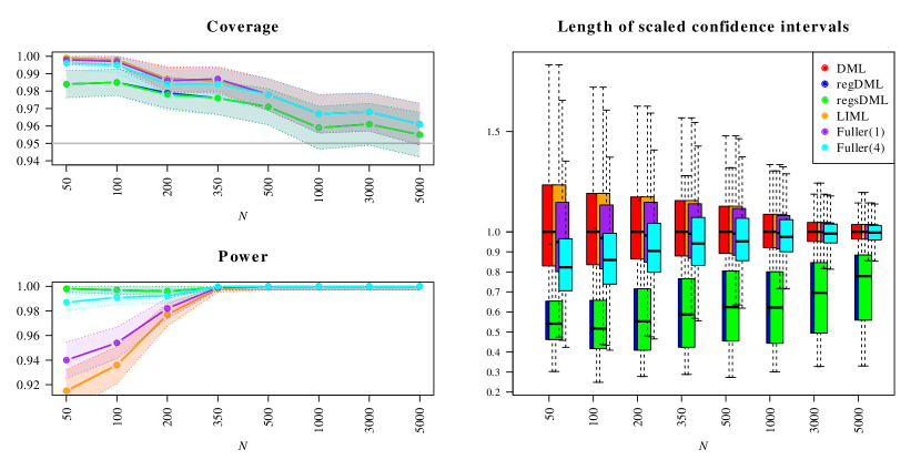
Figure 5: The results come from $M=1000$ simulation runs each from the SEM in Figure 4 for a range of sample sizes $N$ and with $K=2$ and $\mathcal{S}=100$ in Algorithm 1. The nuisance functions are estimated with random forests. The figure displays the coverage of two-sided confidence intervals for $\beta_{0}$, power for two-sided testing of the hypothesis $H_{0}:\ \beta_{0}=0$, and scaled lengths of two-sided confidence intervals of DML (red), regDML (blue), regsDML  (green), LIML (orange), Fuller(1) (purple), and Fuller(4) (cyan), where all results are at level $95\%$. At each $N$, the lengths of the confidence intervals are scaled with the median length from DML. The shaded regions in the coverage and the power plots represent $95\%$ confidence bands with respect to the $M$ simulation runs. The blue and green lines as well as the red and orange ones are indistinguishable in the left panel.

Simulation results with $\beta_{0}=0$ in the SEM in Figure 4 are presented in Figure 8 in the appendix in Section D.

5.2 Real Data Example

We apply the DML and regsDML methods to a real dataset. We estimate the linear effect $\beta_{0}$ of institutions on economic performance following the work of Acemoglu et al. (2001) and Chernozhukov et al. (2018). Countries with better institutions achieve a greater level of income per capita, and wealthy economies can afford better institutions. This may cause simultaneity. To overcome it, mortality rates of the first European settlers in colonies are considered as a source of exogenous variation in institutions. For further details, we refer to Acemoglu et al. (2001) and Chernozhukov et al. (2018). The data is available in the R-package hdm (Chernozhukov et al., 2016) and is called AJR. In our notation, the response $Y$ is the GDP, the covariate $X$ the average protection against expropriation risk, the variable $A$ the logarithm of settler mortality, and the covariate $W$ consists of the latitude, the squared latitude, and the binary factors Africa, Asia, North America, and South America. That is, we adjust nonparametrically for the latitude and geographic information.

We choose $K=2$ and $\mathcal{S}=100$ in Algorithm 1 and compute the conditional expectations with random forests with $1000$ trees that have a minimal node size of $5$. The estimation results are displayed in Table 1. This table gives the estimated linear coefficient, its standard deviation, and a confidence interval for $\beta_{0}$ for DML and regsDML. The coefficient estimate of DML is not significant because the respective confidence interval includes $0$. The regsDML estimate is significant because it has a smaller standard deviation than the DML estimate. Note that the coefficient estimate of regsDML falls within the DML confidence interval.

	Estimate of $\beta_{0}$	Standard error	Confidence interval for $\beta_{0}$
DML	$0.739$	$0.459$	$[-0.161,1.639]$
regsDML	$0.688$	$0.229$	$[0.239,1.136]$

Table 1: Coefficient estimate, its standard error, and a confidence interval with regsDML and DML on the AJR dataset, where $K=2$ and $\mathcal{S}=100$ in Algorithm 1, and where the conditional expectations are estimated with random forests consisting of $1000$ trees that have a minimal node size of $5$.

The AJR dataset has also been analyzed in Chernozhukov et al. (2018). They also estimate conditional expectations with random forests consisting of $1000$ trees that have a minimal node size of $5$ but implicitly assume an additional homoscedasticity condition for the errors $R_{Y}-R_{X}^{T}\beta_{0}$; see Chernozhukov et al. (2017). Such a homoscedastic error assumption is questionable though. Their procedure leads to a smaller estimate of the standard deviation of DML than what we obtain.

6 Conclusion

We extended and regularized double machine learning (DML) in potentially overidentified partially linear models (PLMs) with hidden variables. Our goal was to estimate the linear coefficient $\beta_{0}$ of the PLM. Hidden variables confound the observables, which can cause endogeneity. For instance, a clinical study may experience an endogeneity issue if a treatment is not randomly assigned and subjects receiving different treatments differ in other ways than the treatment (Okui et al., 2012). In such situations, employing estimation methods that do not account for endogeneity lead to biased estimators (Fuller, 1987).

Our contribution was twofold. First, we formulated the PLM as a structural equation model (SEM) and imposed an identifiability condition on it to recover the population parameter $\beta_{0}$. We estimated $\beta_{0}$ using DML similarly to Chernozhukov et al. (2018). However, our setting is more general than the one considered in Chernozhukov et al. (2018) because we allow the predictors to be multivariate, and we impose a moment condition instead of restricting conditional moments. The DML estimation procedure allows biased estimators of additional nuisance functions to be plugged into the estimating equation of $\beta_{0}$. The resulting estimator of $\beta_{0}$ is asymptotically Gaussian and converges at the parametric rate of $N^{-\frac{1}{2}}$. However, DML has a two-stage least squares (TSLS) interpretation and may therefore lead to overly wide confidence intervals.

Second, we proposed a regularization-only DML scheme, regDML, and a regularization-selection DML scheme, regsDML. The latter has shorter confidence intervals by construction because it selects between DML and regDML depending on whose estimated standard deviation is smaller. Although regsDML and plain DML are asymptotically equivalent, regsDML leads to drastically shorter confidence intervals for finite sample sizes. Nevertheless, coverage guarantees for $\beta_{0}$ remain. The regDML estimator is similar to k-class estimation (Theil, 1961) and anchor regression (Rothenhäusler et al., 2021; Bühlmann, 2020; Jakobsen and Peters, 2020) but allows potentially complex partially linear models and chooses a data-driven regularization parameter.

Empirical examples demonstrated our methodological and theoretical developments. The results showed that regsDML is a highly effective method to increase the power and sharpness of statistical inference. The DML estimator has a TSLS interpretation. Therefore, if the confounding is strong, the DML estimator leads to overly wide confidence intervals and can be substantially biased. In such a case, regsDML drastically reduces the width of the confidence intervals but may inherit additional bias from DML. This effect can be particularly pronounced for small sample sizes. Section F in the appendix presents examples with strong and reduced confounding and demonstrates the coverage behavior of DML and regsDML. Section E in the appendix analyzes the performance of our methods if the strength of the link $A\rightarrow X$ varies, and investigates the bias-variance tradeoff of the respective estimated quantities for different values of the regularization parameter.

Although a wide range of machine learners can be employed to estimate the nuisance functions, we observed that additive splines can estimate more precise results than random forests if the underlying structure is additive in good approximation. This effect is particularly pronounced if the sample size is small. If such a finding is to be expected, it may be worthwhile to use structured models rather than “general” machine learning algorithms, especially with small or moderate sample size. Our regsDML methodology can be used with the implementation that is available in the R-package dmlalg (Emmenegger, 2021).

Appendix A An Example where the Identifiability Condition (5) holds, but Conditional Moment Requirements do not

This section presents an SEM where our identifiability condition (5) holds, but where the conditional moment requirements of Chernozhukov et al. (2018) do not.

We assume the model

$$Y\leftarrow X^{T}\beta_{0}+g_{Y}(W)+h_{Y}(H)+\varepsilon_{Y}$$

given in (3) and the identifiability condition $\operatorname{\mathbb{E}}_{P}[R_{A}(R_{Y}-R_{X}^{T}\beta_{0})]=\boldsymbol{0}$ given in (5). Chernozhukov et al. (2018) assume the model

$$Y=X^{T}\beta_{0}+g_{Y}(W)+U,\quad A=g_{A}(W)+V$$ (17)

for unknown functions $g_{Y}$ and $g_{A}$ and impose the conditional moment restrictions

$$\operatorname{\mathbb{E}}[U|A,W]=0\quad\textrm{and}\quad\operatorname{\mathbb{E}}[V|W]=\boldsymbol{0}$$ (18)

on the error terms. Their model is implicitly assumed to be justidentified: the dimensions of $A$ and $X$ are implicitly assumed to be equal.

Model (17) and the conditional moment restrictions (18) imply the identifiability condition (5) due to

$$\operatorname{\mathbb{E}}\big{[}R_{A}(R_{Y}-R_{X}^{T}\beta_{0})\big{]}=\operatorname{\mathbb{E}}\big{[}\big{(}A-g_{A}(W)\big{)}U\big{]}=\operatorname{\mathbb{E}}\big{[}\big{(}A-g_{A}(W)\big{)}\operatorname{\mathbb{E}}[U|A,W]\big{]}=\boldsymbol{0}.$$

However, the reverse direction does not hold. A counterexample is presented in Figure 6 where $W$ directly affects $H$. This SEM satisfies the identifiability condition (5) because $A$ is independent of $H$ conditional on $W$, but it does not satisfy $\operatorname{\mathbb{E}}[U|W,A]=0$ because we have

$$\operatorname{\mathbb{E}}[U|A,W]=\operatorname{\mathbb{E}}[H+\varepsilon_{Y}|A,W]=\operatorname{\mathbb{E}}[H|W]=\operatorname{\mathbb{E}}[W+\varepsilon_{H}|W]=W$$

due to $A\mathchoice{\mathrel{\hbox to0.0pt{$\displaystyle\perp$\hss}\mkern 2.0mu{\displaystyle\perp}}}{\mathrel{\hbox to0.0pt{$\textstyle\perp$\hss}\mkern 2.0mu{\textstyle\perp}}}{\mathrel{\hbox to0.0pt{$\scriptstyle\perp$\hss}\mkern 2.0mu{\scriptstyle\perp}}}{\mathrel{\hbox to0.0pt{$\scriptscriptstyle\perp$\hss}\mkern 2.0mu{\scriptscriptstyle\perp}}}H|W$ and $(\varepsilon_{Y},\varepsilon_{H})\mathchoice{\mathrel{\hbox to0.0pt{$\displaystyle\perp$\hss}\mkern 2.0mu{\displaystyle\perp}}}{\mathrel{\hbox to0.0pt{$\textstyle\perp$\hss}\mkern 2.0mu{\textstyle\perp}}}{\mathrel{\hbox to0.0pt{$\scriptstyle\perp$\hss}\mkern 2.0mu{\scriptstyle\perp}}}{\mathrel{\hbox to0.0pt{$\scriptscriptstyle\perp$\hss}\mkern 2.0mu{\scriptscriptstyle\perp}}}(W,A)$. We have $A\mathchoice{\mathrel{\hbox to0.0pt{$\displaystyle\perp$\hss}\mkern 2.0mu{\displaystyle\perp}}}{\mathrel{\hbox to0.0pt{$\textstyle\perp$\hss}\mkern 2.0mu{\textstyle\perp}}}{\mathrel{\hbox to0.0pt{$\scriptstyle\perp$\hss}\mkern 2.0mu{\scriptstyle\perp}}}{\mathrel{\hbox to0.0pt{$\scriptscriptstyle\perp$\hss}\mkern 2.0mu{\scriptscriptstyle\perp}}}H|W$ because all paths from $A$ to $H$ are blocked by $W$. The path $A\rightarrow X\leftarrow H$ is blocked by the empty set because $X$ is a collider on this path. The path $A\rightarrow X\rightarrow Y\leftarrow H$ is blocked by the empty set because $Y$ is a collider on this path. The path $A\rightarrow X\rightarrow Y\leftarrow W\rightarrow H$ is blocked by $W$. The paths $A\rightarrow X\rightarrow W\rightarrow Y\leftarrow H$ and $A\rightarrow X\rightarrow W\rightarrow H$ are also blocked by $W$.

Figure 6: An SEM and its associated causal graph.

$\displaystyle\begin{array}[]{r}(\varepsilon_{A},\varepsilon_{W},\varepsilon_{H},\varepsilon_{X},\varepsilon_{Y})\sim\mathcal{N}_{5}(\boldsymbol{0},\mathds{1})\\ \end{array}$ $\displaystyle\begin{array}[]{lcl}A&\leftarrow&\varepsilon_{A}\\ W&\leftarrow&\varepsilon_{W}\\ H&\leftarrow&W+\varepsilon_{H}\\ X&\leftarrow&A+W+H+\varepsilon_{X}\\ Y&\leftarrow&X+W+H+\varepsilon_{Y}\end{array}$

Appendix B DML1 Estimators

The DML1 estimators are less preferred than the DML2 estimators we proposed to use in the main text, but for completeness we provide the definitions in this section.

B.1 DML1 Estimator of $\beta_{0}$

The DML1 estimator of $\beta_{0}$ is given by

$$\hat{\beta}^{\textrm{DML1}}:=\frac{1}{K}\sum_{k=1}^{K}\hat{\beta}^{I_{k}},$$

where

$$\hat{\beta}^{I_{k}}:=\Big{(}\big{(}\widehat{\boldsymbol{R}}^{I_{k}}_{\boldsymbol{X}}\big{)}^{T}\Pi_{\widehat{\boldsymbol{R}}^{I_{k}}_{\boldsymbol{A}}}\widehat{\boldsymbol{R}}^{I_{k}}_{\boldsymbol{X}}\Big{)}^{-1}\big{(}\widehat{\boldsymbol{R}}^{I_{k}}_{\boldsymbol{X}}\big{)}^{T}\Pi_{\widehat{\boldsymbol{R}}^{I_{k}}_{\boldsymbol{A}}}\widehat{\boldsymbol{R}}^{I_{k}}_{\boldsymbol{Y}},$$ (19)

and where we recall the projection matrix $\Pi_{\widehat{\boldsymbol{R}}^{I_{k}}_{\boldsymbol{A}}}=\widehat{\boldsymbol{R}}^{I_{k}}_{\boldsymbol{A}}\big{(}(\widehat{\boldsymbol{R}}^{I_{k}}_{\boldsymbol{A}})^{T}\widehat{\boldsymbol{R}}^{I_{k}}_{\boldsymbol{A}}\big{)}^{-1}(\widehat{\boldsymbol{R}}^{I_{k}}_{\boldsymbol{A}})^{T}$ defined in (8). The estimator $\hat{\beta}^{I_{k}}$ is the TSLS estimator of $\widehat{\boldsymbol{R}}^{I_{k}}_{\boldsymbol{Y}}$ on $\widehat{\boldsymbol{R}}^{I_{k}}_{\boldsymbol{X}}$ using the instrument $\widehat{\boldsymbol{R}}^{I_{k}}_{\boldsymbol{A}}$.

B.2 DML1 estimator of $b^{\gamma}$

The DML1 estimator of $b^{\gamma}$ is given by

$$\hat{b}^{\gamma,\textrm{DML1}}:=\frac{1}{K}\sum_{k=1}^{K}\hat{b}^{\gamma}_{k},$$ (20)

where

$$\hat{b}^{\gamma}_{k}:=\operatorname*{arg\,min}_{b\in\mathbb{R}^{d}}\bigg{(}\Big{\lVert}\big{(}\mathds{1}-\Pi_{\widehat{\boldsymbol{R}}^{I_{k}}_{\boldsymbol{A}}}\big{)}\big{(}\widehat{\boldsymbol{R}}^{I_{k}}_{\boldsymbol{Y}}-\big{(}\widehat{\boldsymbol{R}}^{I_{k}}_{\boldsymbol{X}}\big{)}^{T}b\big{)}\Big{\rVert}_{2}^{2}+\gamma\Big{\lVert}\Pi_{\widehat{\boldsymbol{R}}^{I_{k}}_{\boldsymbol{A}}}\big{(}\widehat{\boldsymbol{R}}^{I_{k}}_{\boldsymbol{Y}}-\big{(}\widehat{\boldsymbol{R}}^{I_{k}}_{\boldsymbol{X}}\big{)}^{T}b\big{)}\Big{\rVert}_{2}^{2}\bigg{)}.$$

This estimator can be expressed in closed form by

$$\hat{b}^{\gamma}_{k}=\Big{(}\big{(}\widehat{\boldsymbol{R}}^{I_{k}}_{\widetilde{\boldsymbol{X}}}\big{)}^{T}\widehat{\boldsymbol{R}}^{I_{k}}_{\widetilde{\boldsymbol{X}}}\Big{)}^{-1}\big{(}\widehat{\boldsymbol{R}}^{I_{k}}_{\widetilde{\boldsymbol{X}}}\big{)}^{T}\widehat{\boldsymbol{R}}^{I_{k}}_{\widetilde{\boldsymbol{Y}}},$$

where we recall the notation

$$\widehat{\boldsymbol{R}}^{I_{k}}_{\widetilde{\boldsymbol{X}}}=\Big{(}\mathds{1}+(\sqrt{\gamma}-1)\Pi_{\widehat{\boldsymbol{R}}^{I_{k}}_{\boldsymbol{A}}}\Big{)}\widehat{\boldsymbol{R}}^{I_{k}}_{\boldsymbol{X}}\quad\textrm{and}\quad\widehat{\boldsymbol{R}}^{I_{k}}_{\widetilde{\boldsymbol{Y}}}=\Big{(}\mathds{1}+(\sqrt{\gamma}-1)\Pi_{\widehat{\boldsymbol{R}}^{I_{k}}_{\boldsymbol{A}}}\Big{)}\widehat{\boldsymbol{R}}^{I_{k}}_{\boldsymbol{Y}}$$

as in (15). The computation of $\hat{b}^{\gamma}_{k}$ is an OLS scheme where $\widehat{\boldsymbol{R}}^{I_{k}}_{\widetilde{\boldsymbol{Y}}}$ is regressed on $\widehat{\boldsymbol{R}}^{I_{k}}_{\widetilde{\boldsymbol{X}}}$.

Appendix C SEM of Figure 3

The data from the simulation displayed in Figure 3 come from the following SEM. Let the dimension of $W$ be $v=20$. Let $R$ be the upper triangular matrix of the Cholesky decomposition of the Toeplitz matrix whose first row is given by $(1,0.7,0.7^{2},\ldots,0.7^{19})$. The SEM we consider is given by

$$\begin{array}[]{l}\begin{array}[]{r}(\varepsilon_{A},\varepsilon_{W},\varepsilon_{H},\varepsilon_{X},\varepsilon_{Y})\sim\mathcal{N}_{24}(\boldsymbol{0},\mathds{1})\\ \end{array}\\ \begin{array}[]{lcl}H&\leftarrow&\varepsilon_{H}\\ W&\leftarrow&\varepsilon_{W}R\\ A&\leftarrow&\frac{e^{W_{1}}}{1+e^{W_{1}}}+W_{2}+W_{3}+\varepsilon_{A}\\ X&\leftarrow&2A+W_{1}+0.25\cdot\frac{e^{W_{3}}}{1+e^{W_{3}}}+H+\varepsilon_{X}\\ Y&\leftarrow&X+\frac{e^{W_{1}}}{1+e^{W_{1}}}+0.25W_{3}+H+\varepsilon_{Y}.\end{array}\end{array}$$

Appendix D Additional Numerical Results

If we say in this section that the nuisance parameters are estimated with additive splines, they are estimated with additive cubic B-splines with $\big{\lceil}N^{\frac{1}{5}}\big{\rceil}+2$ degrees of freedom, where $N$ denotes the sample size of the data.

If we say in this section that the nuisance parameters are estimated with random forests, they are estimated with random forests consisting of $500$ trees that have a minimal node size of $5$.

Figure 7 and 8 illustrate the simulation results with $\beta_{0}=0$ of the examples presented in Figure 2 and 5 in Sections 1.1 and 5.1, respectively. The coverage and length of the scaled confidence intervals are similar to the results obtained for $\beta_{0}\neq 0$. Instead of the power as in Figure 2 and 5, Figure 7 and 8 illustrate the type I error.

In Figure 7, DML achieves a type I error of $0$ or close to $0$ over all sample sizes considered. The regsDML method achieves a type I error that is closer to the gray line indicating the $5\%$ level. The dashed lines represent $95\%$ confidence regions. The type I error of regsDML is higher than the type I error of DML because the regsDML confidence intervals are considerably shorter than the DML ones. The right plot in Figure 7 indicates that the lengths of the confidence intervals of regsDML  is around $10\%-30\%$ the length of DML’s. Although regsDML greatly reduces the confidence interval length, the type I error confidence bands include the $5\%$ level or are below it. This means that although regsDML is a regularized version of DML, it does not incur an overlarge bias.

In Figure 8, the type I errors of both DML and regsDML are similar. The $95\%$ confidence regions of both estimators include the $5\%$ level or are below it. The $95\%$ confidence regions of the levels are represented by dashed lines. These confidence regions of both DML and regsDML contain the $5\%$ level or are below it. The right plot in Figure 8 illustrates that the regsDML confidence intervals are around $50\%-80\%$ the length of DML’s. Nevertheless, its type I error does not exceed the $95\%$ level.

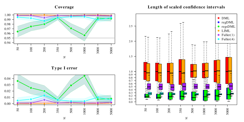
Figure 7: The results come from $M=1000$ simulation runs each from the SEM in Figure 1 with $\beta_{0}=0$ for a range of sample sizes $N$ and with $K=2$ and $\mathcal{S}=100$ in Algorithm 1. The nuisance functions are estimated with additive splines. The figure displays the coverage of two-sided confidence intervals for $\beta_{0}$, type I error for two-sided testing of the hypothesis $H_{0}:\ \beta_{0}=0$, and scaled lengths of two-sided confidence intervals of DML (red), regDML (blue), regsDML  (green), LIML (orange), Fuller(1) (purple), and Fuller(4) (cyan), where all results are at level $95\%$. At each sample size $N$, the lengths of the confidence intervals are scaled with the median length from DML. The shaded regions in the coverage and the type I error plots represent $95\%$ confidence bands with respect to the $M$ simulation runs. The blue and green lines as well as the red and orange ones are indistinguishable in the left panel.

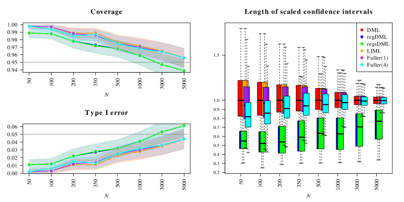
Figure 8: The results come from $M=1000$ simulation runs from the SEM in Figure 4 with $\beta_{0}=0$ for a range of sample sizes $N$ and with $K=2$ and $\mathcal{S}=100$ in Algorithm 1. The nuisance functions are estimated with random forests. The figure displays the coverage of two-sided confidence intervals for $\beta_{0}$, type I error for two-sided testing of the hypothesis $H_{0}:\ \beta_{0}=0$, and scaled lengths of two-sided confidence intervals of DML (red), regDML (blue), regsDML  (green), LIML (orange), Fuller(1) (purple), and Fuller(4) (cyan), where all results are at level $95\%$. At each sample size $N$, the lengths of the confidence intervals are scaled with the median length from DML. The shaded regions in the coverage and the type I error plots represent $95\%$ confidence bands with respect to the $M$ simulation runs. The blue and green lines as well as the red and orange ones are indistinguishable in the left panel.

Appendix E Weak $A\rightarrow X$ and Bias-Variance Tradeoff

First, we analyze the behavior of our methods for varying strength of $A$ on $X$. For $N=200$, we consider the coverage and length of the confidence intervals for varying strength from $A$ to $X$ for the same settings as in Figure 2 and 5.

Figure 9 illustrates the results for data from the SEM from Figure 2. We vary the strength of the direct link $A\rightarrow X$ and denote it by $\alpha$ in Figure 9. Figure 10 illustrates the results for data from the SEM from Figure 5. We leave the link $A_{2}\rightarrow X$ as it is and only vary the strength of the direct link $A_{1}\rightarrow X$, which we denote by $\alpha$ in Figure 10. In both Figure 9 and 10, the coverage remains high for all considered methods. If $\alpha$ becomes larger, the confidence intervals become shorter, which leads to a coverage that is closer to the nominal $95\%$ level, especially in Figure 10. The regsDML method yields the shortest confidence intervals in both figures.

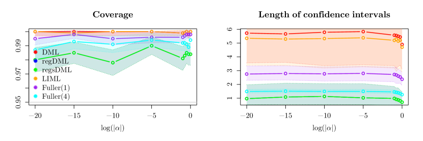
Figure 9: Same setting as in Figure 2, but with $N=200$ only. The strength of the direct link $A\rightarrow X$ varies and is denoted by $\alpha$.

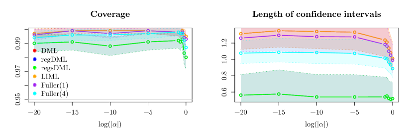
Figure 10: Same setting as in Figure 5, but with $N=200$ only. The strength of the direct link $A_{1}\rightarrow X$ varies and is denoted by $\alpha$.

Second, we analyze the bias-variance tradeoff of the respective estimated quantities of the regularized methods. We again choose the sample size $N=200$ and consider the same settings as in Figure 2 and 5. The results are summarized in Figure 11 and 12 that display the estimated MSE, estimated variance, and estimated squared bias as used in Equation (16). The MSE in both figures is mainly driven by the variance, and regsDML achieves a considerable variance reduction compared to the TSLS-type DML estimator.

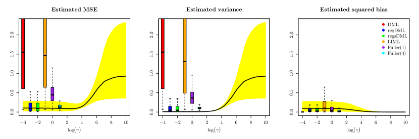
Figure 11: Estimated MSE, estimated variance, and estimated squared bias as used in Equation (16) for the same setting as in Figure 2, but with $N=200$ only. The black solid line displays the median of the respective quantity over the considered range of $\gamma$-values for $\hat{b}^{\gamma}$. The yellow area marks the observed $25\%$ and $75\%$ quantiles. All methods incorporate an additional variance adjustment from the $\mathcal{S}$ repetitions according to Algorithm 1. Boxplots illustrate the performance of the TSLS and the regularized methods. The position of the boxplots is not linked to the $\gamma$-values on the $x$-axis.

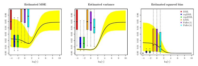
Figure 12: Estimated MSE, estimated variance, and estimated squared bias as used in Equation (16) for the same setting as in Figure 5, but with $N=200$ only. The black solid line displays the median of the respective quantity over the considered range of $\gamma$-values for $\hat{b}^{\gamma}$. The yellow area marks the observed $25\%$ and $75\%$ quantiles. All methods incorporate an additional variance adjustment from the $\mathcal{S}$ repetitions according to Algorithm 1. Boxplots illustrate the performance of the TSLS and the regularized methods. The position of the boxplots is not linked to the $\gamma$-values on the $x$-axis.

Appendix F Confounding and its Mitigation

If we say in this section that the nuisance parameters are estimated with additive splines, they are estimated with additive cubic B-splines with $\big{\lceil}N^{\frac{1}{5}}\big{\rceil}+2$ degrees of freedom, where $N$ denotes the sample size of the data.

If we say in this section that the nuisance parameters are estimated with random forests, they are estimated with random forests consisting of $500$ trees that have a minimal node size of $5$.

We consider models where the DML and the regsDML methods do not work well in terms of coverage of $\beta_{0}$. We present possible explanations of these failures and illustrate model changes to overcome them. The first model in Section F.1 features a strong confounding effect $H\rightarrow X$, the second model in Section F.2 features an effect with noise in $W\rightarrow H$, and the third model in Section F.3 features an effect with noise in $H\rightarrow W$.

F.1 Strong Confounding Effect $H\rightarrow X$

If the hidden variable $H$ is strongly confounded with $X$, the resulting TSLS-type DML estimator can be substantially biased depending on the choice of functions in the model. If the estimated variances are not large enough, the coverage of the resulting confidence intervals for $\beta_{0}$ can be too low. This issue is illustrated in Figure 14.

The regsDML estimator mimics the bias behavior of DML because the DML estimator is used as a replacement of $\beta_{0}$ in the MSE objective function that defines the estimated regularization parameter of regDML in (16). The confidence intervals of regsDML  are shorter than the DML ones, but both are computed with a similarly biased coefficient estimate of $\beta_{0}$. Therefore, the coverage of the confidence intervals of regsDML  is even worse than the one of DML.

The coverages of both DML and regsDML are considerably improved if the confounding strength is reduced; see Figure 15.

Figure 13: An SEM and its associated causal graph.

$\displaystyle\begin{array}[]{r}(\varepsilon_{A},\varepsilon_{W},\varepsilon_{H},\varepsilon_{X},\varepsilon_{Y})\sim\mathcal{N}_{5}(\boldsymbol{0},\mathds{1})\\ \end{array}$ $\displaystyle\begin{array}[]{lcl}A&\leftarrow&\varepsilon_{A}\\ W&\leftarrow&\varepsilon_{W}\\ H&\leftarrow&\varepsilon_{H}\\ X&\leftarrow&A+W+\chi H+0.25\varepsilon_{X}\\ Y&\leftarrow&\beta_{0}X+W+H+0.25\varepsilon_{Y}\end{array}$

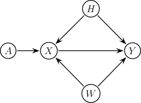
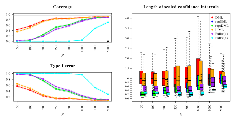
Figure 14: The results come from $M=1000$ simulation runs from the SEM in Figure 13 with $\chi=15$ and $\beta_{0}=0$ for a range of sample sizes $N$ and with $K=2$ and $\mathcal{S}=100$ in Algorithm 1. The nuisance functions are estimated with additive splines. The figure displays the coverage of two-sided confidence intervals for $\beta_{0}$, type I error for two-sided testing of the hypothesis $H_{0}:\ \beta_{0}=0$, and scaled lengths of two-sided confidence intervals of DML (red), regDML (blue), regsDML  (green), LIML (orange), Fuller(1) (purple), and Fuller(4) (cyan), where all results are at level $95\%$. At each sample size $N$, the lengths of the confidence intervals are scaled with the median length from DML. The shaded regions in the coverage and the type I error plots represent $95\%$ confidence bands with respect to the $M$ simulation runs. The blue and green lines are indistinguishable in the left panel.

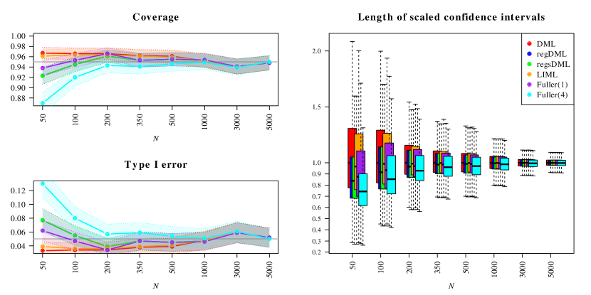
Figure 15: The results come from $M=1000$ simulation runs from the SEM in Figure 13 with $\chi=1$ and $\beta_{0}=0$ for a range of sample sizes $N$ and with $K=2$ and $\mathcal{S}=100$ in Algorithm 1. The nuisance functions are estimated with additive splines. The figure displays the coverage of two-sided confidence intervals for $\beta_{0}$, type I error for two-sided testing of the hypothesis $H_{0}:\ \beta_{0}=0$, and scaled lengths of two-sided confidence intervals of DML (red), regDML (blue), regsDML  (green), LIML (orange), Fuller(1) (purple), and Fuller(4) (cyan), where all results are at level $95\%$. At each sample size $N$, the lengths of the confidence intervals are scaled with the median length from DML. The shaded regions in the coverage and the type I error plots represent $95\%$ confidence bands with respect to the $M$ simulation runs. The blue and green lines are indistinguishable in the left panel.

F.2 Noise in $W\rightarrow H$

The variable $W$ may have a direct effect on $H$. If this link is strong enough with respect to the additional noise $\varepsilon_{H}$ of $H$, it is possible to obtain some information of $H$ by observing $W$. This can reduce the overall level of confounding present depending on the choice of functions in the model.

Simulation results where $W$ explains only part of the variation in $H$ are presented in Figure 17. The confidence intervals of both DML and regsDML do not attain a $95\%$ coverage for small sample sizes $N$. The situation can be considerably improved by reducing the variation of $H$ that is not explained by $W$; see Figure 18.

Figure 16: An SEM and its associated causal graph.

$\displaystyle\begin{array}[]{r}(\varepsilon_{A},\varepsilon_{W},\varepsilon_{H},\varepsilon_{X},\varepsilon_{Y})\sim\mathcal{N}_{5}(\boldsymbol{0},\mathds{1})\\ \end{array}$ $\displaystyle\begin{array}[]{lcl}A&\leftarrow&\varepsilon_{A}\\ W&\leftarrow&\varepsilon_{W}\\ H&\leftarrow&W+\kappa\varepsilon_{H}\\ X&\leftarrow&0.5A+3\tanh(2W)+1.5H+0.25\varepsilon_{X}\\ Y&\leftarrow&\beta_{0}X-\tanh(W)+H+0.25\varepsilon_{Y}\end{array}$

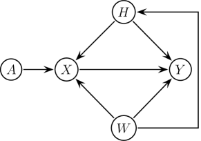
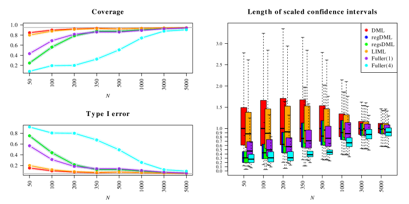
Figure 17: The results come from $M=1000$ simulation runs from the SEM in Figure 16 with $\kappa=2$ and $\beta_{0}=0$ for a range of sample sizes $N$ and with $K=2$ and $\mathcal{S}=100$ in Algorithm 1. The nuisance functions are estimated with additive splines. The figure displays the coverage of two-sided confidence intervals for $\beta_{0}$, type I error for two-sided testing of the hypothesis $H_{0}:\ \beta_{0}=0$, and scaled lengths of two-sided confidence intervals of DML (red), regDML (blue), regsDML  (green), LIML (orange), Fuller(1) (purple), and Fuller(4) (cyan), where all results are at level $95\%$. At each sample size $N$, the lengths of the confidence intervals are scaled with the median length from DML. The shaded regions in the coverage and the type I error plots represent $95\%$ confidence bands with respect to the $M$ simulation runs. The blue and green lines are indistinguishable in the left panel.

Figure 18: The results come from $M=1000$ simulation runs from the SEM in Figure 16 with $\kappa=0.25$ and $\beta_{0}=0$ for a range of sample sizes $N$ and with $K=2$ and $\mathcal{S}=100$ in Algorithm 1. The figure displays the coverage of two-sided confidence intervals for $\beta_{0}$, type I error for two-sided testing of the hypothesis $H_{0}:\ \beta_{0}=0$, and scaled lengths of two-sided confidence intervals of DML (red), regDML (blue), regsDML  (green), LIML (orange), Fuller(1) (purple), and Fuller(4) (cyan), where all results are at level $95\%$, and where the nuisance functions are estimated with additive splines. At each sample size $N$, the lengths of the confidence intervals are scaled with the median length from DML. The shaded regions in the coverage and the type I error plots represent $95\%$ confidence bands with respect to the $M$ simulation runs. The blue and green lines are indistinguishable in the left panel.

F.3 Noise in $H\rightarrow W$

The variable $H$ may have a direct effect on $W$. If this link is strong enough with respect to the additional noise $\varepsilon_{W}$ of $W$, it is possible to obtain some information of $H$ by observing $W$ similarly to Section F.2. The results again depend on the choice of functions in the model.

Figure 20 presents simulation results where $H$ explains only little variation of $W$ compared with $\varepsilon_{W}$. The confidence intervals of regsDML do not attain a $95\%$ coverage for small sample sizes $N$ because the estimator inherits additional bias from DML. The situation can be improved by reducing the variation of $W$ that is not explained by $H$; see Figure 21.

Figure 19: An SEM and its associated causal graph.

$\displaystyle\begin{array}[]{r}(\varepsilon_{H},\varepsilon_{W},\varepsilon_{A},\varepsilon_{X},\varepsilon_{Y})\sim\mathcal{N}_{5}(\boldsymbol{0},\mathds{1})\\ \end{array}$ $\displaystyle\begin{array}[]{lcl}H&\leftarrow&\varepsilon_{H}\\ W&\leftarrow&2H+\kappa\varepsilon_{W}\\ A&\leftarrow&e^{-0.5W}+0.5\varepsilon_{A}\\ X&\leftarrow&-A-0.1W^{3}-0.2W^{2}+0.4W\\ &&\quad+\frac{7}{1+e^{-4H}}+0.25\varepsilon_{X}\\ Y&\leftarrow&\beta_{0}X+0.5W+0.5H+\varepsilon_{Y}\end{array}$

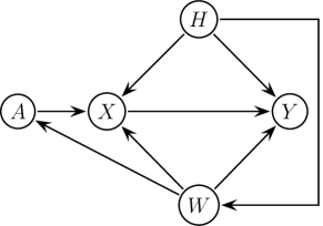
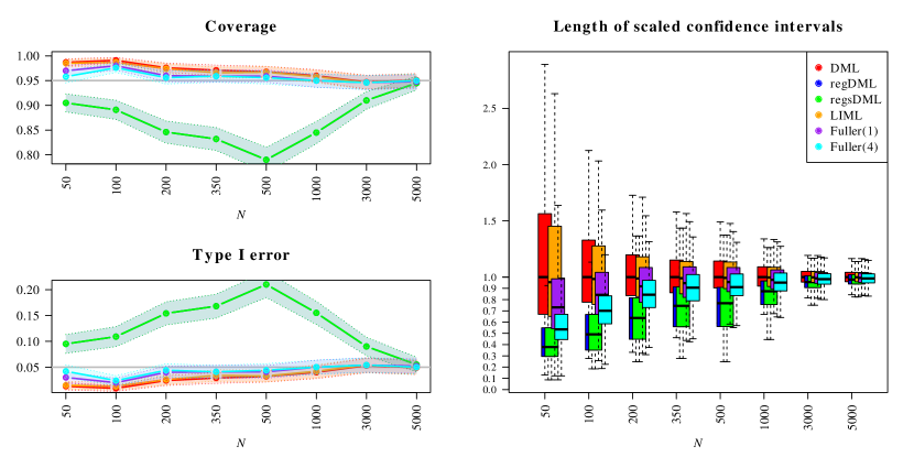
Figure 20: The results come from $M=1000$ simulation runs from the SEM in Figure 19 with $\kappa=1$ and $\beta_{0}=0$ for a range of sample sizes $N$ and with $K=2$ and $\mathcal{S}=100$ in Algorithm 1. The nuisance functions are estimated with additive splines. The figure displays the coverage of two-sided confidence intervals for $\beta_{0}$, type I error for two-sided testing of the hypothesis $H_{0}:\ \beta_{0}=0$, and scaled lengths of two-sided confidence intervals of DML (red), regDML (blue), regsDML  (green), LIML (orange), Fuller(1) (purple), and Fuller(4) (cyan), where all results are at level $95\%$. At each sample size $N$, the lengths of the confidence intervals are scaled with the median length from DML. The shaded regions in the coverage and the type I error plots represent $95\%$ confidence bands with respect to the $M$ simulation runs. The blue and green lines are indistinguishable in the left panel.

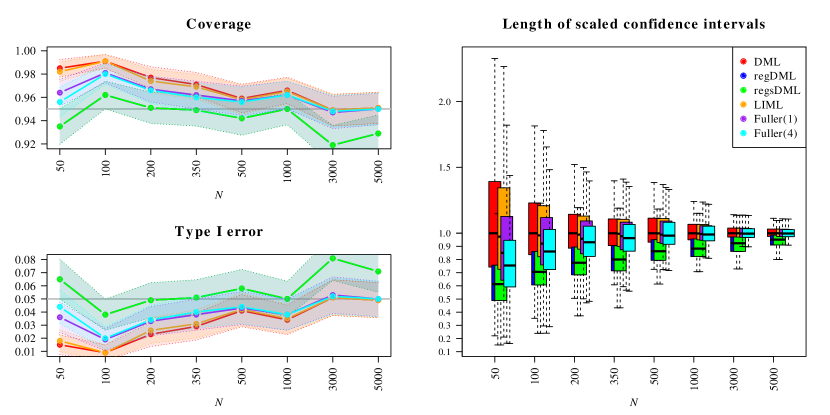
Figure 21: The results come from $M=1000$ simulation runs from the SEM in Figure 19 with $\kappa=0.25$ and $\beta_{0}=0$ for a range of sample sizes $N$ and with $K=2$ and $\mathcal{S}=100$ in Algorithm 1. The nuisance functions are estimated with additive splines. The figure displays the coverage of two-sided confidence intervals for $\beta_{0}$, type I error for two-sided testing of the hypothesis $H_{0}:\ \beta_{0}=0$, and scaled lengths of two-sided confidence intervals of DML (red), regDML (blue), regsDML  (green), LIML (orange), Fuller(1) (purple), and Fuller(4) (cyan), where all results are at level $95\%$. At each sample size $N$, the lengths of the confidence intervals are scaled with the median length from DML. The shaded regions in the coverage and the type I error plots represent $95\%$ confidence bands with respect to the $M$ simulation runs. The blue and green lines are indistinguishable in the left panel.

Appendix G Examples where the identifiability condition (5) does and does not hold

The following examples illustrate SEMs where the identifiability condition (5) holds and where it fails to hold. We argue using causal graphs; see Lauritzen (1996); Pearl (1998, 2009, 2010); Peters et al. (2017); Maathuis et al. (2019). By convention, we omit error variables in a causal graph if they are assumed to be mutually independent (Pearl, 2009).

Example G.1.

Consider the SEM of the 1-dimensional variables $A$, $W$, $H$, $X$, and $Y$ and its associated causal graph given in Figure 22, where $\beta_{0}$ is a fixed unknown parameter, and where $a_{W}$, $a_{X}$, $g_{Y}$, $g_{H}$, $h_{X}$, and $h_{Y}$ are some appropriate functions. The variable $A$ directly influences $W$, and $W$ directly influences the hidden variable $H$. The variable $A$ is independent of $H$ given $W$ because every path from $A$ to $H$ is blocked by $W$; a proof is given in the appendix in Section H.

Figure 22: An SEM satisfying the identifiability condition (5) and its associated causal graph as in Example G.1.

$\displaystyle\begin{array}[]{r}\varepsilon_{A},\varepsilon_{W},\varepsilon_{H},\varepsilon_{X},\varepsilon_{Y}\end{array}$ $\displaystyle\begin{array}[]{lcl}A&\leftarrow&\varepsilon_{A}\\ W&\leftarrow&a_{W}(A)+\varepsilon_{W}\\ H&\leftarrow&g_{H}(W)+\varepsilon_{H}\\ X&\leftarrow&a_{X}(A)+h_{X}(H)+\varepsilon_{X}\\ Y&\leftarrow&\beta_{0}X+g_{Y}(W)+h_{Y}(H)+\varepsilon_{Y}\end{array}$

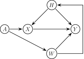
Proof of Example G.1.

The path $A\rightarrow X\leftarrow H$ is blocked by the empty set because $X$ is a collider on this path. The paths $A\rightarrow\cdots\rightarrow Y\leftarrow H$ are blocked by the empty set because $Y$ is a collider on these paths. The path $A\rightarrow W\rightarrow H$ is blocked by $W$. ∎

The variable $A$ is exogenous in Example G.1. In general, this is no requirement; see Example G.2.

Example G.2.

Consider the SEM of the 1-dimensional variables $H$, $W$, $A$, $X$, and $Y$ and its associated causal graph given in Figure 23, where $\beta_{0}$ is a fixed unknown parameter, and where $a_{X}$, $g_{A}$, $g_{X}$, $g_{Y}$, $h_{X}$, $h_{W}$, and $h_{Y}$ are some appropriate functions. The variable $A$ is not a source node. The hidden variable $H$ directly influences $W$, and $W$ directly influences $A$. The variable $A$ is independent of $H$ given $W$ because every path from $A$ to $H$ is blocked by $W$; a proof is given in the appendix in Section H.

Figure 23: An SEM satisfying the identifiability condition (5) and its associated causal graph as in Example G.2.

$\displaystyle\begin{array}[]{r}\varepsilon_{H},\varepsilon_{W},\varepsilon_{A},\varepsilon_{X},\varepsilon_{Y}\end{array}$ $\displaystyle\begin{array}[]{lcl}H&\leftarrow&\varepsilon_{H}\\ W&\leftarrow&h_{W}(H)+\varepsilon_{W}\\ A&\leftarrow&g_{A}(W)+\varepsilon_{A}\\ X&\leftarrow&a_{X}(A)+g_{X}(W)+h_{X}(H)+\varepsilon_{X}\\ Y&\leftarrow&\beta_{0}X+g_{Y}(W)+h_{Y}(H)+\varepsilon_{Y}\end{array}$

Proof of Example G.2.

The path $A\rightarrow X\leftarrow H$ is blocked by the empty set because $X$ is a collider on this path. The paths $A\rightarrow X\rightarrow\cdots\rightarrow Y\leftarrow H$ are blocked by the empty set because $Y$ is a collider on these paths. The paths $A\leftarrow W\rightarrow Y\leftarrow X\leftarrow H$, $A\leftarrow W\leftarrow H$, and $A\rightarrow X\leftarrow W\leftarrow H$ are blocked by $W$. The path $A\leftarrow W\rightarrow Y\leftarrow H$ is blocked by $W$ or alternatively by the empty set because $Y$ is a collider on this path. The path $A\leftarrow W\rightarrow X\leftarrow H$ is blocked by $W$ or alternatively by the empty set because $X$ is a collider on this path. ∎

Identifiability of $\beta_{0}$ is not guaranteed if $A$ and $H$ are independent. An illustration is given in Example G.3. Considering the instrument $A$ instead of $R_{A}$ in Theorem 2.1 cannot solve the issue. In such a situation, stronger structural assumptions are required.

Example G.3.

Consider the SEM of the 1-dimensional variables $H$, $A$, $W$, $X$, and $Y$ and its associated causal graph given in Figure 24, where $\beta_{0}$ is a fixed unknown parameter. Although $A$ and $H$ are independent, the identifiability condition (5) does not hold; a proof is given in the appendix in Section H.

Figure 24: An SEM not satisfying the identifiability condition (5) together with its associated causal graph as in Example G.3

$\displaystyle\begin{array}[]{r}(\varepsilon_{H},\varepsilon_{A},\varepsilon_{W},\varepsilon_{X},\varepsilon_{Y})\sim\mathcal{N}_{5}(0,\mathds{1})\end{array}$ $\displaystyle\begin{array}[]{lcl}H&\leftarrow&\varepsilon_{H}\\ A&\leftarrow&\varepsilon_{A}\\ W&\leftarrow&A+H+\varepsilon_{W}\\ X&\leftarrow&A+W+H+\varepsilon_{X}\\ Y&\leftarrow&\beta_{0}X+W+H+\varepsilon_{Y}\end{array}$

Proof of Example G.3.

The two random variables $A$ and $H$ are independent because the path $A\rightarrow W\leftarrow H$ is not blocked by $W$. Indeed, $W$ is a collider on this path.

All random variables are 1-dimensional. Therefore, the representation of $\beta_{0}$ in Theorem 2.1 is equivalent to the identifiability condition

$$\operatorname{\mathbb{E}}[R_{A}(R_{Y}-R_{X}\beta_{0})]=0$$

in Equation (5). However, the identifiability condition does not hold in the present situation. We have

$$\begin{array}[]{cl}&\operatorname{\mathbb{E}}[R_{A}(R_{Y}-R_{X}\beta_{0})]\\ =&\operatorname{\mathbb{E}}[R_{A}\big{(}H+\varepsilon_{Y}-\operatorname{\mathbb{E}}[H+\varepsilon_{Y}|W]\big{)}\big{]}\\ =&\operatorname{\mathbb{E}}\big{[}R_{A}\big{(}H-\operatorname{\mathbb{E}}[H|W]\big{)}\big{]}\end{array}$$

because $\varepsilon_{Y}$ is independent of $A$ and $W$ and centered. By the tower property for conditional expectations, we have

$$\begin{array}[]{cl}\operatorname{\mathbb{E}}[R_{A}(R_{Y}-R_{X}\beta_{0})]=\operatorname{\mathbb{E}}\big{[}AH-A\operatorname{\mathbb{E}}[H|W]\big{]}.\end{array}$$

Because $A$ and $H$ are independent and centered, we have $\operatorname{\mathbb{E}}[AH]=0$. Moreover, we have $H\sim\mathcal{N}(0,1)$, $W\sim\mathcal{N}(0,3)$, and $(W|H=h)\sim\mathcal{N}(h,2)$. The conditional distribution of $H|W=w$ can be obtained by applying Bayes’ theorem and is given by $\mathcal{N}(\frac{1}{3}w,\frac{2}{3})$. Hence, we have $\operatorname{\mathbb{E}}[H|W]=\frac{1}{3}W$ and

$$\operatorname{\mathbb{E}}\big{[}A\operatorname{\mathbb{E}}[H|W]\big{]}=\frac{1}{3}\operatorname{\mathbb{E}}[AW]=\frac{1}{3}\operatorname{\mathbb{E}}\big{[}A^{2}\big{]}=\frac{1}{3}\neq 0$$

because $A$ is independent of $H$ and $\varepsilon_{W}$. Therefore, we have $\operatorname{\mathbb{E}}[R_{A}(R_{Y}-R_{X}\beta_{0})]\neq 0$ and $\beta_{0}$ cannot be represented as in Theorem 2.1. ∎

Appendix H Proofs of Section 2

Proof of Theorem 2.1.

To prove the theorem, we need to verify

$$\beta_{0}=\Big{(}\operatorname{\mathbb{E}}\big{[}R_{X}R_{A}^{T}\big{]}\operatorname{\mathbb{E}}\big{[}R_{A}R_{A}^{T}\big{]}^{-1}\operatorname{\mathbb{E}}\big{[}R_{A}R_{X}^{T}\big{]}\Big{)}^{-1}\operatorname{\mathbb{E}}\big{[}R_{X}R_{A}^{T}\big{]}\operatorname{\mathbb{E}}\big{[}R_{A}R_{A}^{T}\big{]}^{-1}\operatorname{\mathbb{E}}[R_{A}R_{Y}].$$

This statement is equivalent to

$$\boldsymbol{0}=\operatorname{\mathbb{E}}\big{[}R_{X}R_{A}^{T}\big{]}\operatorname{\mathbb{E}}\big{[}R_{A}R_{A}^{T}\big{]}^{-1}\operatorname{\mathbb{E}}\big{[}R_{A}\big{(}R_{Y}-R_{X}^{T}\beta_{0})\big{]}.$$

This last statement holds because $\operatorname{\mathbb{E}}[R_{A}(R_{Y}-R_{X}^{T}\beta_{0})]$ equals $\boldsymbol{0}$ due to the identifiability condition (5). ∎

Appendix I Proofs of Section 3

We denote by $\lVert\cdot\rVert$ either the Euclidean norm for a vector or the operator norm for a matrix.

Proof of Proposition 3.3.

We have

$$\begin{array}[]{cl}&\frac{\partial}{\partial r}\Big{|}_{r=0}\operatorname{\mathbb{E}}_{P}\big{[}\psi\big{(}S;\beta_{0},\eta^{0}+r(\eta-\eta^{0})\big{)}\big{]}\\ =&\frac{\partial}{\partial r}\Big{|}_{r=0}\operatorname{\mathbb{E}}_{P}\bigg{[}\Big{(}A-m_{A}^{0}(W)-r\big{(}m_{A}(W)-m_{A}^{0}(W)\big{)}\Big{)}\\ &\quad\quad\quad\cdot\bigg{(}Y-m_{Y}^{0}(W)-r\big{(}m_{Y}(W)-m_{Y}^{0}(W)\big{)}\\ &\quad\quad\quad\quad\quad-\Big{(}X-m_{X}^{0}(W)-r\big{(}m_{X}(W)-m_{X}^{0}(W)\big{)}\Big{)}^{T}\beta_{0}\bigg{)}\bigg{]}\\ =&\operatorname{\mathbb{E}}_{P}\Big{[}-\big{(}m_{A}(W)-m_{A}^{0}(W)\big{)}\Big{(}Y-m_{Y}^{0}(W)-\big{(}X-m_{X}^{0}(W)\big{)}^{T}\beta_{0}\Big{)}\\ &\quad\quad\quad\quad+\big{(}A-m_{A}^{0}(W)\big{)}\Big{(}-\big{(}m_{Y}(W)-m_{Y}^{0}(W)\big{)}+\big{(}m_{X}(W)-m_{X}^{0}(W)\big{)}^{T}\beta_{0}\Big{)}\Big{]}.\end{array}$$

Subsequently, we show that both terms

$$\operatorname{\mathbb{E}}_{P}\Big{[}\big{(}m_{A}(W)-m_{A}^{0}(W)\big{)}\Big{(}Y-m_{Y}^{0}(W)-\big{(}X-m_{X}^{0}(W)\big{)}^{T}\beta_{0}\Big{)}\Big{]}$$ (21)

and

$$\operatorname{\mathbb{E}}_{P}\Big{[}\big{(}A-m_{A}^{0}(W)\big{)}\Big{(}-\big{(}m_{Y}(W)-m_{Y}^{0}(W)\big{)}+\big{(}m_{X}(W)-m_{X}^{0}(W)\big{)}^{T}\beta_{0}\Big{)}\Big{]}$$ (22)

are equal to $\boldsymbol{0}$. We first consider the term (21). Recall the notations $m_{Y}^{0}(W)=\operatorname{\mathbb{E}}_{P}[Y|W]$ and $m_{X}^{0}(W)=\operatorname{\mathbb{E}}_{P}[X|W]$. We have

$$\begin{array}[]{cl}&\operatorname{\mathbb{E}}_{P}\Big{[}\big{(}m_{A}(W)-m_{A}^{0}(W)\big{)}\Big{(}Y-m_{Y}^{0}(W)-\big{(}X-m_{X}^{0}(W)\big{)}^{T}\beta_{0}\Big{)}\Big{]}\\ =&\operatorname{\mathbb{E}}_{P}\Big{[}\big{(}m_{A}(W)-m_{A}^{0}(W)\big{)}\operatorname{\mathbb{E}}_{P}\big{[}Y-\operatorname{\mathbb{E}}_{P}[Y|W]-(X-\operatorname{\mathbb{E}}_{P}[X|W])^{T}\beta_{0}\big{|}W\big{]}\Big{]}\\ =&\boldsymbol{0}.\end{array}$$

Next, we verify that the term given in (22) vanishes. Recall the notation $m_{A}^{0}(W)=\operatorname{\mathbb{E}}_{P}[A|W]$. We have

$$\begin{array}[]{cl}&\operatorname{\mathbb{E}}_{P}\Big{[}\big{(}A-m_{A}^{0}(W)\big{)}\Big{(}-\big{(}m_{Y}(W)-m_{Y}^{0}(W)\big{)}+\big{(}m_{X}(W)-m_{X}^{0}(W)\big{)}^{T}\beta_{0}\Big{)}\Big{]}\\ =&\operatorname{\mathbb{E}}_{P}\Big{[}\operatorname{\mathbb{E}}_{P}\big{[}A-\operatorname{\mathbb{E}}[A|W]\big{|}W\big{]}\Big{(}-\big{(}m_{Y}(W)-m_{Y}^{0}(W)\big{)}+\big{(}m_{X}(W)-m_{X}^{0}(W)\big{)}^{T}\beta_{0}\Big{)}\Big{]}\\ =&\boldsymbol{0}.\end{array}$$

Because both terms (21) and (22) vanish, we conclude

$$\frac{\partial}{\partial r}\Big{|}_{r=0}\operatorname{\mathbb{E}}_{P}\big{[}\psi\big{(}S;\beta_{0},\eta^{0}+r(\eta-\eta^{0})\big{)}\big{]}=\boldsymbol{0}.$$

∎

Definition I.1.

Consider a set $\mathcal{T}$ of nuisance functions. For $S=(A,X,W,Y)$, an element $\eta=(m_{A},m_{X},m_{Y})\in\mathcal{T}$, and $\beta\in\mathbb{R}^{d}$, we introduce the score functions

$$\widetilde{\psi}(S,\beta,\eta):=\big{(}X-m_{X}(W)\big{)}\Big{(}Y-m_{Y}(W)-\big{(}X-m_{X}(W)\big{)}^{T}\beta\Big{)},$$ (23)

and

$$\begin{array}[]{rcl}\psi_{1}(S,\eta)&:=&\big{(}X-m_{X}(W)\big{)}\big{(}A-m_{A}(W)\big{)}^{T},\\ \psi_{2}(S,\eta)&:=&\big{(}A-m_{A}(W)\big{)}\big{(}A-m_{A}(W)\big{)}^{T},\\ \psi_{3}(S,\eta)&:=&\big{(}X-m_{X}(W)\big{)}\big{(}X-m_{X}(W)\big{)}^{T}.\end{array}$$

Furthermore, let the matrices

$$\begin{array}[]{rcl}D_{1}&:=&\operatorname{\mathbb{E}}_{P}[\psi_{3}(S;\eta^{0})],\\ D_{2}&:=&\operatorname{\mathbb{E}}_{P}[\psi_{1}(S;\eta^{0})]\operatorname{\mathbb{E}}_{P}[\psi_{2}(S;\eta^{0})]^{-1}\operatorname{\mathbb{E}}_{P}\big{[}\psi_{1}^{T}(S;\eta^{0})\big{]},\\ D_{3}&:=&\operatorname{\mathbb{E}}_{P}[\psi_{1}(S;\eta^{0})]\operatorname{\mathbb{E}}_{P}[\psi_{2}(S;\eta^{0})]^{-1},\\ D_{5}&:=&\operatorname{\mathbb{E}}_{P}[\psi_{2}(S;\eta^{0})]^{-1}\operatorname{\mathbb{E}}_{P}[\psi(S;b^{\gamma},\eta^{0})],\\ J_{0}&:=&D_{2}^{-1}D_{3},\\ \tilde{J}_{0}&:=&\operatorname{\mathbb{E}}_{P}\big{[}\psi(S;\beta_{0},\eta^{0})\psi^{T}(S;\beta_{0},\eta^{0})\big{]}=\operatorname{\mathbb{E}}\big{[}R_{A}R_{A}^{T}(R_{Y}-R_{X}^{T}\beta_{0})^{2}\big{]},\\ J_{0}^{\prime\prime}&:=&\operatorname{\mathbb{E}}_{P}[R_{A}R_{A}^{T}],\\ J_{0}^{\prime}&:=&\operatorname{\mathbb{E}}_{P}\big{[}R_{X}(R_{A})^{T}\big{]}(J_{0}^{\prime\prime})^{-1}\operatorname{\mathbb{E}}_{P}\big{[}R_{A}(R_{X})^{T}\big{]}\end{array}$$

and the variance-covariance matrix $\sigma^{2}:=J_{0}\tilde{J}_{0}J_{0}^{T}$. Moreover, let the score function

$$\overline{\psi}(\cdot;\beta_{0},\eta^{0}):=\sigma^{-1}\tilde{J}_{0}^{-\frac{1}{2}}\psi(\cdot;\beta_{0},\eta^{0}).$$

Definition I.2.

Let $\gamma\geq 0$. Consider a realization set $\mathcal{T}$ of nuisance functions. Define the statistical rates

$$r_{N}^{4}:=\max_{\begin{subarray}{c}S=(U,V,W,Z)\in\{A,X,Y\}^{2}\times\{W\}\times\{A,X,Y\},\\ b^{0}\in\{b^{\gamma},\beta_{0},\boldsymbol{0}\}\end{subarray}}\sup_{\eta\in\mathcal{T}}\operatorname{\mathbb{E}}_{P}[\lVert\psi(S;b^{0},\eta)-\psi(S;b^{0},\eta^{0})\rVert],$$

$$\lambda_{N}:=\max_{\begin{subarray}{c}\varphi\in\{\psi,\widetilde{\psi},\psi_{2}\}^{,}\\ b^{0}\in\{b^{\gamma},\beta_{0},\boldsymbol{0}\}\end{subarray}}\sup_{r\in(0,1),\eta\in\mathcal{T}}\big{\lVert}\partial_{r}^{2}\operatorname{\mathbb{E}}_{P}\big{[}\varphi\big{(}S;b^{0},\eta^{0}+r(\eta-\eta^{0})\big{)}\big{]}\big{\rVert},$$

where we interpret $\psi_{2}\big{(}S;b^{0},\eta^{0}+r(\eta-\eta^{0})\big{)}$ as $\psi_{2}\big{(}S;\eta^{0}+r(\eta-\eta^{0})\big{)}$ in the definition of $\lambda_{N}$.

Remark I.3.

We would like to remark that the respective definition of the statistical rate $r_{N}$ given in Chernozhukov et al. (2018) involves the $L_{2}$-norm of $\psi(S;b^{0},\eta)-\psi(S;b^{0},\eta^{0})$ instead of its $L_{1}$-norm. However, it is essential to employ the $L_{1}$-norm to ensure that Assumption I.5.5 can constrain the $L_{2}$-norm of the estimation errors incurred by the ML estimators of the nuisance parameters. Thus, we do not have to constrain their higher order errors to employ Hölder’s inequality in Lemma I.16.

Definition I.4.

Let the nonrandom numbers

$$\rho_{N}:=r_{N}+N^{\frac{1}{2}}\lambda_{N}\quad\textrm{and}\quad\tilde{\rho}_{N}:=N^{\max\big{\{}\frac{4}{p}-1,-\frac{1}{2}\big{\}}}+r_{N}.$$

If not stated otherwise, we assume the following Assumption I.5 in all the results presented in the appendix.

Assumptions I.5.

Let $\gamma\geq 0$. Let $K\geq 2$ be a fixed integer independent of $N$. We assume that $N\geq K$ holds. Let $\{\delta_{N}\}_{N\geq K}$ and $\{\Delta_{N}\}_{N\geq K}$ be two sequences of positive numbers that converge to zero, where $\delta_{N}^{\frac{1}{4}}\geq N^{-\frac{1}{2}}$ holds. Let $\{\mathcal{P}_{N}\}_{N\geq 1}$ be a sequence of sets of probability distributions $P$ of the quadruple $S=(A,W,X,Y)$.

Let $p>4$. For all $N$, for all $P\in\mathcal{P}_{N}$, consider a nuisance function realization sets $\mathcal{T}$ such that the following conditions hold:

1. We have an SEM given by (3) that satisfies the identifiability conditon (5).

2. There exists a finite real constant $C_{1}$ satisfying $\lVert A\rVert_{P,p}+\lVert X\rVert_{P,p}+\lVert Y\rVert_{P,p}\leq C_{1}$.

3. The matrix $\operatorname{\mathbb{E}}_{P}[R_{X}R_{A}^{T}]\in\mathbb{R}^{d\times q}$ has full rank $d$. This in particular requires $q\geq d$. The matrices $D_{1}\in\mathbb{R}^{d\times d}$ and $J_{0}^{\prime\prime}\in\mathbb{R}^{q\times q}$ are invertible. Furthermore, the smallest and largest singular values of the symmetric matrices $J_{0}^{\prime\prime}$ and $J_{0}^{\prime}$ are bounded away from $0$ by $c_{1}>0$ and are bounded away from $+\infty$ by $c_{2}<\infty$.

4. The symmetric matrices $\tilde{J}_{0}$, $D_{1}+(\gamma-1)D_{2}$, and $D_{4}$ are invertible, where $D_{4}$ is introduced in Definition J.1 in the appendix in Section J. The smallest and largest singular values of these matrices are bounded away from $0$ by $c_{3}$ and are bounded away from $+\infty$ by $c_{4}$.

5. The set $\mathcal{T}$ consists of $P$-integrable functions $\eta=(m_{A},m_{X},m_{Y})$ whose $p$th moment exists and it contains $\eta^{0}$. There exists a finite real constant $C_{2}$ such that

   $$\begin{array}[]{l}\lVert\eta^{0}-\eta\rVert_{P,p}\leq C_{2},\quad\lVert\eta^{0}-\eta\rVert_{P,2}\leq\delta_{N},\quad\lVert m_{A}^{0}(W)-m_{A}(W)\rVert_{P,2}^{2}\leq\delta_{N}N^{-\frac{1}{2}},\\ \lVert m_{X}^{0}(W)-m_{X}(W)\rVert_{P,2}\big{(}\lVert m_{Y}^{0}(W)-m_{Y}(W)\rVert_{P,2}+\lVert m_{X}^{0}(W)-m_{X}(W)\rVert_{P,2}\big{)}\leq\delta_{N}N^{-\frac{1}{2}},\\ \lVert m_{A}^{0}(W)-m_{A}(W)\rVert_{P,2}\big{(}\lVert m_{Y}^{0}(W)-m_{Y}(W)\rVert_{P,2}+\lVert m_{X}^{0}(W)-m_{X}(W)\rVert_{P,2}\big{)}\leq\delta_{N}N^{-\frac{1}{2}}\end{array}$$

   hold for all elements $\eta$ of $\mathcal{T}$. Given a partition $I_{1},\ldots,I_{K}$ of $[N]$ where each $I_{k}$ is of size $n=\frac{N}{K}$, for all $k\in[K]$, the nuisance parameter estimate $\hat{\eta}^{I_{k}^{c}}=\hat{\eta}^{I_{k}^{c}}(\{S_{i}\}_{i\in I_{k}^{c}})$ satisfies

   $$\begin{array}[]{l}\lVert\eta^{0}-\hat{\eta}^{I_{k}^{c}}\rVert_{P,p}\leq C_{2},\quad\lVert\eta^{0}-\hat{\eta}^{I_{k}^{c}}\rVert_{P,2}\leq\delta_{N},\quad\lVert m_{A}^{0}(W)-\hat{m}_{A}^{I_{k}^{c}}(W)\rVert_{P,2}^{2}\leq\delta_{N}N^{-\frac{1}{2}},\\ \lVert m_{X}^{0}(W)-\hat{m}_{X}^{I_{k}^{c}}(W)\rVert_{P,2}\big{(}\lVert m_{Y}^{0}(W)-\hat{m}_{Y}^{I_{k}^{c}}(W)\rVert_{P,2}+\lVert m_{X}^{0}(W)-\hat{m}_{X}^{I_{k}^{c}}(W)\rVert_{P,2}\big{)}\leq\delta_{N}N^{-\frac{1}{2}},\\ \lVert m_{A}^{0}(W)-\hat{m}_{A}^{I_{k}^{c}}(W)\rVert_{P,2}\big{(}\lVert m_{Y}^{0}(W)-\hat{m}_{Y}^{I_{k}^{c}}(W)\rVert_{P,2}+\lVert m_{X}^{0}(W)-\hat{m}_{X}^{I_{k}^{c}}(W)\rVert_{P,2}\big{)}\leq\delta_{N}N^{-\frac{1}{2}}\end{array}$$

   with $P$-probability no less than $1-\Delta_{N}$. Denote by $\mathcal{E}_{N}$ the event that $\hat{\eta}^{I_{k}^{c}}=\hat{\eta}^{I_{k}^{c}}(\{S_{i}\}_{i\in I_{k}^{c}})$ belongs to $\mathcal{T}$ and assume that this event holds with $P$-probability no less than $1-\Delta_{N}$.

For instance, invertibility of the square matrices $\operatorname{\mathbb{E}}_{P}[R_{A}R_{A}^{T}]$ and $\tilde{J}_{0}$ is satisfied if $\varepsilon_{Y}$ is independent of both $A$ and $W$ and has a strictly positive variance.

Remark I.6.

It is possible to drop some of the assumptions in Assumption I.5 if we are interested in proving the results about DML only. The full assumption is required to prove the results about both DML and regDML.

We assume Assumption I.5 throughout.

Lemma I.7.

Let $u\geq 1$. Consider a $t$-dimensional random variable $Z$. Denote the joint law of $Z$ and $W$ by $P$. Then we have

$$\lVert Z-\operatorname{\mathbb{E}}_{P}[Z|W]\rVert_{P,{u}}\leq 2\lVert Z\rVert_{P,u}.$$

Proof of Lemma I.7.

Because the Euclidean norm to the $u$th power is convex for ${u}\geq 1$, we have

$$\lVert\operatorname{\mathbb{E}}_{P}[Z|W]\rVert_{P,u}^{u}=\operatorname{\mathbb{E}}_{P}\big{[}\lVert\operatorname{\mathbb{E}}_{P}[Z|W]\rVert^{u}\big{]}\leq\operatorname{\mathbb{E}}_{P}\big{[}\operatorname{\mathbb{E}}_{P}[\lVert Z\rVert^{u}|W]\big{]}=\operatorname{\mathbb{E}}_{P}[\lVert Z\rVert^{u}]=\lVert Z\rVert_{P,{u}}^{u}$$

by Jensen’s inequality. We hence have

$$\begin{array}[]{rcl}\lVert Z-\operatorname{\mathbb{E}}_{P}[Z|W]\rVert_{P,{u}}\leq\lVert Z\rVert_{P,{u}}+\lVert\operatorname{\mathbb{E}}_{P}[Z|W]\rVert_{P,{u}}\leq 2\lVert Z\rVert_{P,{u}}\end{array}$$

by the triangle inequality. ∎

Lemma I.8.

Consider a $t$-dimensional random variable $Z$. Denote the joint law of $Z$ and $W$ by $P$. Then we have

$$\big{\lVert}\operatorname{\mathbb{E}}_{P}\big{[}ZZ^{T}-\operatorname{\mathbb{E}}_{P}[Z|W]\operatorname{\mathbb{E}}_{P}[Z^{T}|W]\big{]}\big{\rVert}\leq 2\lVert Z\rVert_{P,2}^{2}.$$

Proof of Lemma I.8.

Because the Euclidean norm is convex, we have

$$\begin{array}[]{rcl}\big{\lVert}\operatorname{\mathbb{E}}_{P}\big{[}ZZ^{T}-\operatorname{\mathbb{E}}_{P}[Z|W]\operatorname{\mathbb{E}}_{P}[Z^{T}|W]\big{]}\big{\rVert}&\leq&\operatorname{\mathbb{E}}_{P}\big{[}\lVert ZZ^{T}\rVert+\lVert\operatorname{\mathbb{E}}_{P}[Z|W]\operatorname{\mathbb{E}}_{P}[Z^{T}|W]\rVert\big{]}\\ &\leq&\operatorname{\mathbb{E}}_{P}\big{[}\lVert Z\rVert^{2}+\lVert\operatorname{\mathbb{E}}_{P}[Z|W]\rVert^{2}\big{]}\\ \end{array}$$

by Jensen’s inequality, the triangle inequality and the Cauchy–Schwarz inequality. Because the squared Euclidean norm is convex, we have

$$\lVert\operatorname{\mathbb{E}}_{P}[Z|W]\rVert^{2}\leq\operatorname{\mathbb{E}}_{P}\big{[}\lVert Z\rVert^{2}\big{|}W\big{]}$$

by Jensen’s inequality. Therefore, we have

$$\begin{array}[]{rcl}\big{\lVert}\operatorname{\mathbb{E}}_{P}\big{[}ZZ^{T}-\operatorname{\mathbb{E}}_{P}[Z|W]\operatorname{\mathbb{E}}_{P}[Z^{T}|W]\big{]}\big{\rVert}&\leq&\operatorname{\mathbb{E}}_{P}\big{[}\lVert Z\rVert^{2}+\lVert\operatorname{\mathbb{E}}_{P}[Z|W]\rVert^{2}\big{]}\\ &\leq&\operatorname{\mathbb{E}}_{P}\big{[}\lVert Z\rVert^{2}+\operatorname{\mathbb{E}}_{P}[\lVert Z\rVert^{2}|W]\big{]}\\ &=&2\lVert Z\rVert_{P,2}^{2}.\end{array}$$

∎

Lemma I.9.

Consider a $t_{1}$-dimensional random variable $Z_{1}$ and a $t_{2}$-dimensional random variable $Z_{2}$. Denote the joint law of $Z_{1}$, $Z_{2}$, and $W$ by $P$. Then we have

$$\big{\lVert}\operatorname{\mathbb{E}}_{P}\big{[}(Z_{1}-\operatorname{\mathbb{E}}_{P}[Z_{1}|W])(Z_{2}-\operatorname{\mathbb{E}}_{P}[Z_{2}|W])^{T}\big{]}\big{\rVert}^{2}\leq\lVert Z_{1}\rVert_{P,2}^{2}\lVert Z_{2}\rVert_{P,2}^{2}.$$

Proof of Lemma I.9.

By the Cauchy–Schwarz inequality, we have

$$\begin{array}[]{cl}&\big{\lVert}\operatorname{\mathbb{E}}_{P}\big{[}(Z_{1}-\operatorname{\mathbb{E}}_{P}[Z_{1}|W])(Z_{2}-\operatorname{\mathbb{E}}_{P}[Z_{2}|W])^{T}\big{]}\big{\rVert}^{2}\\ \leq&\operatorname{\mathbb{E}}_{P}\big{[}\lVert(Z_{1}-\operatorname{\mathbb{E}}_{P}[Z_{1}|W])\rVert^{2}\big{]}\operatorname{\mathbb{E}}_{P}\big{[}\lVert(Z_{2}-\operatorname{\mathbb{E}}_{P}[Z_{2}|W])\rVert^{2}\big{]}.\end{array}$$

Because the conditional expectation minimizes the mean squared error (Durrett, 2010, Theorem 5.1.8), we have

$$\operatorname{\mathbb{E}}_{P}\big{[}\lVert(Z_{1}-\operatorname{\mathbb{E}}_{P}[Z_{1}|W])\rVert^{2}\big{]}\leq\lVert Z_{1}\rVert_{P,2}^{2}$$

and

$$\operatorname{\mathbb{E}}_{P}\big{[}\lVert(Z_{2}-\operatorname{\mathbb{E}}_{P}[Z_{2}|W])\rVert^{2}\big{]}\leq\lVert Z_{2}\rVert_{P,2}^{2}.$$

In total, we thus have

$$\big{\lVert}\operatorname{\mathbb{E}}_{P}\big{[}(Z_{1}-\operatorname{\mathbb{E}}_{P}[Z_{1}|W])(Z_{2}-\operatorname{\mathbb{E}}_{P}[Z_{2}|W])^{T}\big{]}\big{\rVert}^{2}\leq\lVert Z_{1}\rVert_{P,2}^{2}\lVert Z_{2}\rVert_{P,2}^{2}.$$

∎

Lemma I.10.

Consider a $t_{1}$-dimensional random variable $Z_{1}$ and a $t_{2}$-dimensional random variable $Z_{2}$. Denote the joint law of $Z_{1}$, $Z_{2}$, and $W$ by $P$. Then we have

$$\big{\lVert}\operatorname{\mathbb{E}}_{P}\big{[}(Z_{1}-\operatorname{\mathbb{E}}_{P}[Z_{1}|W])Z_{2}^{T}\big{]}\big{\rVert}^{2}\leq\lVert Z_{1}\rVert_{P,2}^{2}\lVert Z_{2}\rVert_{P,2}^{2}.$$

Proof of Lemma I.10.

By the Cauchy–Schwarz inequality, we have

$$\big{\lVert}\operatorname{\mathbb{E}}_{P}\big{[}(Z_{1}-\operatorname{\mathbb{E}}_{P}[Z_{1}|W])Z_{2}^{T}\big{]}\big{\rVert}^{2}\leq\operatorname{\mathbb{E}}_{P}\big{[}\lVert Z_{1}-\operatorname{\mathbb{E}}_{P}[Z_{1}|W]\rVert^{2}\big{]}\operatorname{\mathbb{E}}_{P}\big{[}\lVert Z_{2}\rVert^{2}\big{]}.$$

Because the conditional expectation minimizes the mean squared error (Durrett, 2010, Theorem 5.1.8), we have

$$\operatorname{\mathbb{E}}_{P}\big{[}\lVert Z_{1}-\operatorname{\mathbb{E}}_{P}[Z_{1}|W]\rVert^{2}\big{]}\leq\operatorname{\mathbb{E}}_{P}\big{[}\lVert Z_{1}\rVert^{2}\big{]}=\lVert Z_{1}\rVert_{P,2}^{2}.$$

Consequently,

$$\big{\lVert}\operatorname{\mathbb{E}}_{P}\big{[}(Z_{1}-\operatorname{\mathbb{E}}_{P}[Z_{1}|W])Z_{2}^{T}\big{]}\big{\rVert}^{2}\leq\lVert Z_{1}\rVert_{P,2}^{2}\lVert Z_{2}\rVert_{P,2}^{2}$$

holds. ∎

Lemma I.11.

Let $a,b\in\mathbb{R}$ be two numbers. We have

$$(a+b)^{2}\leq 2a^{2}+2b^{2}.$$ (24)

Proof of Lemma I.11.

The true statement $0\leq(a-b)^{2}$ is equivalent to (24). ∎

The following lemma proved in Chernozhukov et al. (2018) states that conditional convergence in probability implies unconditional convergence in probability.

Lemma I.12.

(Based on Chernozhukov et al. (2018, Lemma 6.1).) Let $\{X_{t}\}_{t\geq 1}$ and $\{Y_{t}\}_{t\geq 1}$ be sequences of random vectors and let ${u}\geq 1$. Consider a deterministic sequence $\{\varepsilon_{t}\}_{t\geq 1}$ with $\varepsilon_{t}\rightarrow 0$ as $t\rightarrow\infty$ such that we have $\operatorname{\mathbb{E}}[\lVert X_{t}\rVert^{u}|Y_{t}]\leq\varepsilon_{t}^{u}$. Then we have $\lVert X_{t}\rVert=O_{P}(\varepsilon_{t})$ unconditionally, meaning that that for any sequence $\{\ell_{t}\}_{t\geq 1}$ with $\ell_{t}\rightarrow\infty$ as $t\rightarrow\infty$ we have $P(\lVert X_{t}\rVert>\ell_{t}\varepsilon_{t})\rightarrow 0$.

Proof of Lemma I.12.

We have

$$P(\lVert X_{t}\rVert>\ell_{t}\varepsilon_{t})=\operatorname{\mathbb{E}}[P(\lVert X_{t}\rVert>\ell_{t}\varepsilon_{t}|Y_{t})]\leq\frac{\operatorname{\mathbb{E}}\big{[}\operatorname{\mathbb{E}}[\lVert X_{t}\rVert^{u}|Y_{t}]\big{]}}{\ell_{t}^{u}\varepsilon_{t}^{u}}\leq\frac{1}{\ell_{t}^{u}}\rightarrow 0\quad(t\rightarrow\infty)$$

by Markov’s inequality. ∎

Lemma I.13.

There exists a finite real constant $C_{3}$ satisfying $\lVert\beta_{0}\rVert\leq C_{3}$.

Proof of Lemma I.13.

Recall the matrices $J_{0}^{\prime}$ and $J_{0}^{\prime\prime}$ in Definition I.1. We have

$$\begin{array}[]{rcl}\lVert\beta_{0}\rVert&\leq&\big{\lVert}(J_{0}^{\prime})^{-1}\big{\rVert}\big{\lVert}\operatorname{\mathbb{E}}_{P}\big{[}A(R_{X})^{T}\big{]}\big{\rVert}\big{\lVert}(J_{0}^{\prime\prime})^{-1}\big{\rVert}\big{\lVert}\operatorname{\mathbb{E}}_{P}\big{[}AR_{Y}\big{]}\big{\rVert}\\ &\leq&\frac{1}{c_{2}^{2}}\lVert X\rVert_{P,2}\lVert Y\rVert_{P,2}\lVert A\rVert_{P,2}^{2}\end{array}$$

by submultiplicativity, Assumption I.5.3, and Lemma I.10. We hence infer

$$\lVert\beta_{0}\rVert\leq\frac{1}{c_{2}^{2}}C_{1}^{4}$$

by Assumption I.5.2. ∎

Lemma I.14.

Let $\gamma\geq 0$. There exists a finite real constant $C_{4}$ satisfying $\lVert b^{\gamma}\rVert\leq C_{4}$.

Proof of Lemma I.14.

We have

$$\begin{array}[]{rcl}\lVert b^{\gamma}\rVert&\leq&\Big{\lVert}\Big{(}\operatorname{\mathbb{E}}_{P}\big{[}R_{X}R_{X}^{T}\big{]}+(\gamma-1)\operatorname{\mathbb{E}}_{P}\big{[}R_{X}R_{A}^{T}\big{]}\operatorname{\mathbb{E}}_{P}\big{[}R_{A}R_{A}^{T}\big{]}^{-1}\operatorname{\mathbb{E}}_{P}\big{[}R_{A}R_{X}^{T}\big{]}\Big{)}^{-1}\Big{\rVert}\\ &&\quad\cdot\Big{\lVert}\operatorname{\mathbb{E}}_{P}[R_{X}R_{Y}]+(\gamma-1)\operatorname{\mathbb{E}}_{P}\big{[}R_{X}R_{A}^{T}\big{]}\operatorname{\mathbb{E}}_{P}\big{[}R_{A}R_{A}^{T}\big{]}^{-1}\operatorname{\mathbb{E}}_{P}[R_{A}R_{Y}]\Big{\rVert}\end{array}$$

by submultiplicativity. By Assumption I.5.4, the largest singular value of the matrix

$$D_{1}+(\gamma-1)D_{2}=\operatorname{\mathbb{E}}_{P}\big{[}R_{X}R_{X}^{T}\big{]}+(\gamma-1)\operatorname{\mathbb{E}}_{P}\big{[}R_{X}R_{A}^{T}\big{]}\operatorname{\mathbb{E}}_{P}\big{[}R_{A}R_{A}^{T}\big{]}^{-1}\operatorname{\mathbb{E}}_{P}\big{[}R_{A}R_{X}^{T}\big{]}$$

is upper bounded by $0<c_{4}<\infty$. Thus, we have

$$\lVert b^{\gamma}\rVert\leq\frac{1}{c_{4}}\Big{(}\lVert\operatorname{\mathbb{E}}_{P}[R_{X}R_{Y}]\rVert+\lvert\gamma-1\rvert\big{\lVert}\operatorname{\mathbb{E}}_{P}\big{[}R_{X}R_{A}^{T}\big{]}\big{\rVert}\Big{\lVert}\operatorname{\mathbb{E}}_{P}\big{[}R_{A}R_{A}^{T}\big{]}^{-1}\Big{\rVert}\big{\lVert}\operatorname{\mathbb{E}}_{P}\big{[}R_{A}R_{Y}^{T}\big{]}\big{\rVert}\Big{)}$$

by the triangle inequality and submultiplicativity. By Assumption I.5.3, the largest singular value of $\operatorname{\mathbb{E}}_{P}[R_{A}R_{A}^{T}]$ is upper bounded by $0<c_{2}<\infty$. By Lemma I.9 and Assumption I.5.2, we have

$$\begin{array}[]{l}\big{\lVert}\operatorname{\mathbb{E}}_{P}\big{[}R_{X}R_{Y}\big{]}\big{\rVert}\leq\lVert X\rVert_{P,2}\lVert Y\rVert_{P,2}\leq C_{1}^{2},\\ \big{\lVert}\operatorname{\mathbb{E}}_{P}\big{[}R_{X}R_{A}^{T}\big{]}\big{\rVert}\leq\lVert X\rVert_{P,2}\lVert A\rVert_{P,2}\leq C_{1}^{2},\\ \big{\lVert}\operatorname{\mathbb{E}}_{P}\big{[}R_{A}R_{Y}^{T}\big{]}\big{\rVert}\leq\lVert A\rVert_{P,2}\lVert Y\rVert_{P,2}\leq C_{1}^{2}.\end{array}$$

In total, we hence have

$$\lVert b^{\gamma}\rVert\leq\frac{1}{c_{4}}\bigg{(}C_{1}^{2}+\lvert\gamma-1\rvert\frac{C_{1}^{4}}{c_{2}}\bigg{)}.$$

∎

Lemma I.15.

Let $\gamma\geq 0$ The statistical rates $r_{N}$ and $\lambda_{N}$ introduced in Definition I.2 satisfy $r_{N}^{4}\lesssim\delta_{N}$ and $\lambda_{N}\lesssim\frac{\delta_{N}}{\sqrt{N}}$.

Proof of Lemma I.15.

This proof is modified from Chernozhukov et al. (2018). First, verify the bound on $r_{N}$. Let $S=(U,V,W,Z)\in\{A,X,Y\}^{2}\times\{W\}\times\{A,X,Y\}$, let $\eta=(m_{U},m_{V},m_{Z})\in\mathcal{T}$, and let $b^{0}\in\{b^{\gamma},\beta_{0},\boldsymbol{0}\}$. We have

$$\begin{array}[]{cl}&\psi(S;b^{0},\eta)-\psi(S;b^{0},\eta^{0})\\ =&\big{(}U-m_{U}(W)\big{)}\Big{(}Z-m_{Z}(W)-\big{(}V-m_{V}(W)\big{)}^{T}b^{0}\Big{)}^{T}\\ &\quad-\big{(}U-m_{U}^{0}(W)\big{)}\Big{(}Z-m_{Z}^{0}(W)-\big{(}V-m_{V}^{0}(W)\big{)}^{T}b^{0}\Big{)}^{T}\\ =&\big{(}U-m_{U}^{0}(W)\big{)}\Big{(}m_{Z}^{0}(W)-m_{Z}(W)-\big{(}m_{V}^{0}(W)-m_{V}(W)\big{)}^{T}b^{0}\Big{)}^{T}\\ &\quad+\big{(}m_{U}^{0}(W)-m_{U}(W)\big{)}\Big{(}Z-m_{Z}^{0}(W)-\big{(}V-m_{V}^{0}(W)\big{)}^{T}b^{0}\Big{)}^{T}\\ &\quad+\big{(}m_{U}^{0}(W)-m_{U}(W)\big{)}\Big{(}m_{Z}^{0}(W)-m_{Z}(W)-\big{(}m_{V}^{0}(W)-m_{V}(W)\big{)}^{T}b^{0}\Big{)}^{T}.\end{array}$$

By the triangle inequality and Hölder’s inequality, we have

$$\begin{array}[]{cl}&\operatorname{\mathbb{E}}_{P}[\lVert\psi(S;b^{0},\eta)-\psi(S;b^{0},\eta^{0})\rVert]\\ =&\lVert\psi(S;b^{0},\eta)-\psi(S;b^{0},\eta^{0})\rVert_{P,1}\\ \leq&\lVert U-m_{U}^{0}(W)\rVert_{P,2}\Big{\lVert}m_{Z}^{0}(W)-m_{Z}(W)-\big{(}m_{V}^{0}(W)-m_{V}(W)\big{)}^{T}b^{0}\Big{\rVert}_{P,2}\\ &\quad+\lVert m_{U}^{0}(W)-m_{U}(W)\rVert_{P,2}\Big{\lVert}Z-m_{Z}^{0}(W)-\big{(}V-m_{V}^{0}(W)\big{)}^{T}b^{0}\Big{\rVert}_{P,2}\\ &\quad+\lVert m_{U}^{0}(W)-m_{U}(W)\rVert_{P,2}\Big{\lVert}m_{Z}^{0}(W)-m_{Z}(W)-\big{(}m_{V}^{0}(W)-m_{V}(W)\big{)}^{T}b^{0}\Big{\rVert}_{P,2}.\end{array}$$

Observe that $\lVert U-m_{U}^{0}(W)\rVert_{P,2}\leq 2\lVert U\rVert_{P,2}$, and $\lVert V-m_{V}^{0}(W)\rVert_{P,2}\leq 2\lVert V\rVert_{P,2}$, and $\lVert Z-m_{Z}^{0}(W)\rVert_{P,2}\leq 2\lVert Z\rVert_{P,2}$ hold by Lemma I.7. We have $\lVert\eta-\eta^{0}\rVert_{P,2}\leq\delta_{N}$ by Assumption I.5.5. Therefore, we obtain the upper bound

$$\begin{array}[]{cl}&\operatorname{\mathbb{E}}_{P}[\lVert\psi(S;b^{0},\eta)-\psi(S;b^{0},\eta^{0})\rVert]\\ \leq&4\max\{1,\lVert b^{0}\rVert\}(\lVert U\rVert_{P,2}+\lVert V\rVert_{P,2}+\lVert Z\rVert_{P,2})\delta_{N}+2\max\{1,\lVert b^{0}\rVert\}\delta_{N}^{2}\\ \lesssim&\delta_{N}\end{array}$$

by the triangle inequality, Lemma I.13, Lemma I.14, and Assumptions I.5.2 and I.5.5. Because this upper bound is independent of $\eta$, we obtain our claimed bound on $r_{N}^{4}$.

Subsequently, we verify the bound on $\lambda_{N}$. Consider $S=(A,X,W,Y)$, denote by $U$ either $A$ or $X$, denote by $Z$ either $A$ or $Y$, and let $\varphi\in\{\psi,\widetilde{\psi},\psi_{2}\}$, where we interpret $\psi_{2}(S;b,\eta)=\psi_{2}(S;\eta)$. We have

$$\begin{array}[]{cl}&\partial_{r}^{2}\operatorname{\mathbb{E}}_{P}\big{[}\psi\big{(}S;b^{0},\eta^{0}+r(\eta-\eta^{0})\big{)}\big{]}\\ =&2\operatorname{\mathbb{E}}_{P}\bigg{[}\big{(}m_{U}(W)-m_{U}^{0}(W)\big{)}\Big{(}m_{Z}(W)-m_{Z}^{0}(W)-\big{(}m_{X}(W)-m_{X}^{0}(W)\big{)}^{T}b^{0}\Big{)}^{T}\bigg{]}.\end{array}$$

Due to the Cauchy–Schwarz inequality, we infer

$$\begin{array}[]{cl}&\big{\lVert}\partial_{r}^{2}\operatorname{\mathbb{E}}_{P}\big{[}\psi\big{(}S;b^{0},\eta^{0}+r(\eta-\eta^{0})\big{)}\big{]}\big{\rVert}\\ \leq&2\lVert m_{U}(W)-m_{U}^{0}(W)\rVert_{P,2}\big{(}\lVert m_{Z}(W)-m_{Z}^{0}(W)\rVert_{P,2}+\lVert m_{X}(W)-m_{X}^{0}(W)\rVert_{P,2}\lVert b^{0}\rVert\big{)}\\ \leq&2\max\{1,\lVert b^{0}\rVert\}\lVert m_{U}(W)-m_{U}^{0}(W)\rVert_{P,2}\\ &\quad\cdot\big{(}\lVert m_{Z}(W)-m_{Z}^{0}(W)\rVert_{P,2}+\lVert m_{X}(W)-m_{X}^{0}(W)\rVert_{P,2}\big{)}\\ \lesssim&\delta_{N}N^{-\frac{1}{2}}\end{array}$$

by Lemma I.13, Lemma I.14, and Assumption I.5.5. Consequently, we obtain our claimed bound on $\lambda_{N}$. ∎

Lemma I.16.

Let $\gamma\geq 0$. Let $k\in[K]$. Let furthermore $\varphi\in\{\psi,\widetilde{\psi},\psi_{2}\}$ and $b^{0}\in\{b^{\gamma},\beta_{0},\boldsymbol{0}\}$. We have

$$\bigg{\lVert}\frac{1}{\sqrt{n}}\sum_{i\in I_{k}}\varphi(S_{i};b^{0},\hat{\eta}^{I_{k}^{c}})-\frac{1}{\sqrt{n}}\sum_{i\in I_{k}}\varphi(S_{i};b^{0},\eta^{0})\bigg{\rVert}=O_{P}(\rho_{N}),$$

where $\rho_{N}=r_{N}+N^{\frac{1}{2}}\lambda_{N}$ is as in Definition I.4 and satisfies $\rho_{N}\lesssim\delta_{N}^{\frac{1}{4}}$, and where we interpret $\psi_{2}(S;b,\eta)=\psi_{2}(S;\eta)$.

Proof of Lemma I.16.

This proof is modified from Chernozhukov et al. (2018). By the triangle inequality, we have

$$\begin{array}[]{cl}&\Big{\lVert}\frac{1}{\sqrt{n}}\sum_{i\in I_{k}}\varphi(S_{i};b^{0},\hat{\eta}^{I_{k}^{c}})-\frac{1}{\sqrt{n}}\sum_{i\in I_{k}}\varphi(S_{i};b^{0},\eta^{0})\Big{\rVert}\\ =&\Big{\lVert}\frac{1}{\sqrt{n}}\sum_{i\in I_{k}}\big{(}\varphi(S_{i};b^{0},\hat{\eta}^{I_{k}^{c}})-\int\varphi(s;b^{0},\hat{\eta}^{I_{k}^{c}})\mathrm{d}P(s)\big{)}\\ &\quad\quad-\frac{1}{\sqrt{n}}\sum_{i\in I_{k}}\big{(}\varphi(S_{i};b^{0},\eta^{0})-\int\varphi(s;b^{0},\eta^{0})\mathrm{d}P(s)\big{)}\\ &\quad\quad+\sqrt{n}\int\big{(}\varphi(s;b^{0},\hat{\eta}^{I_{k}^{c}})-\varphi(s;b^{0},\eta^{0})\big{)}\mathrm{d}P(s)\Big{\rVert}\\ \leq&\mathcal{I}_{1}+\sqrt{n}\mathcal{I}_{2},\end{array}$$

where $\mathcal{I}_{1}:=\lVert M\rVert$ for

$$\begin{array}[]{rcl}M&:=&\frac{1}{\sqrt{n}}\sum_{i\in I_{k}}\bigg{(}\varphi(S_{i};b^{0},\hat{\eta}^{I_{k}^{c}})-\int\varphi(s;b^{0},\hat{\eta}^{I_{k}^{c}})\mathrm{d}P(s)\bigg{)}\\ &&\quad-\frac{1}{\sqrt{n}}\sum_{i\in I_{k}}\bigg{(}\varphi(S_{i};b^{0},\eta^{0})-\int\varphi(s;b^{0},\eta^{0})\mathrm{d}P(s)\bigg{)},\end{array}$$

and where

$$\mathcal{I}_{2}:=\bigg{\lVert}\int\big{(}\varphi(s;b^{0},\hat{\eta}^{I_{k}^{c}})-\varphi(s;b^{0},\eta^{0})\big{)}\mathrm{d}P(s)\bigg{\rVert}.$$

We bound the two terms $\mathcal{I}_{1}$ and $\mathcal{I}_{2}$ individually. First, we bound $\mathcal{I}_{1}$. Because the dimensions $d$ and $q$ are fixed, it is sufficient to bound one entry of the matrix $M$. Let $l$ index the rows of $M$ and let $t$ index the columns of $M$ (we interpret vectors as matrices with one column). On the event $\mathcal{E}_{N}$ the that holds with $P$-probability $1-\Delta_{N}$, we have

$$\begin{array}[]{cl}&\operatorname{\mathbb{E}}_{P}\big{[}\lVert M_{l,t}\rVert^{2}\big{|}\{S_{i}\}_{i\in I_{k}^{c}}\big{]}\\ =&\frac{1}{n}\sum_{i\in I_{k}}\operatorname{\mathbb{E}}_{P}\big{[}\lvert\varphi_{l,t}(S_{i};b^{0},\hat{\eta}^{I_{k}^{c}})-\varphi_{l,t}(S_{i};b^{0},\eta^{0})\rvert^{2}\big{|}\{S_{i}\}_{i\in I_{k}^{c}}\big{]}\\ &\quad+\frac{1}{n}\sum_{i,j\in I_{k},i\neq j}\operatorname{\mathbb{E}}_{P}\big{[}\big{(}\varphi_{l,t}(S_{i};b^{0},\hat{\eta}^{I_{k}^{c}})-\varphi_{l,t}(S_{i};b^{0},\eta^{0})\big{)}\\ &\quad\quad\quad\quad\quad\quad\quad\quad\quad\quad\quad\cdot\big{(}\varphi_{l,t}(S_{j};b^{0},\hat{\eta}^{I_{k}^{c}})-\varphi_{l,t}(S_{j};b^{0},\eta^{0})\big{)}\big{|}\{S_{i}\}_{i\in I_{k}^{c}}\big{]}\\ &\quad-2\sum_{i\in I_{k}}\operatorname{\mathbb{E}}_{P}\big{[}\varphi_{l,t}(S_{i};b^{0},\hat{\eta}^{I_{k}^{c}})-\varphi_{l,t}(S_{i};b^{0},\eta^{0})\big{|}\{S_{i}\}_{i\in I_{k}^{c}}\big{]}\\ &\quad\quad\quad\quad\quad\quad\cdot\operatorname{\mathbb{E}}_{P}\big{[}\varphi_{l,t}(S;b^{0},\hat{\eta}^{I_{k}^{c}})-\varphi_{l,t}(S;b^{0},\eta^{0})\big{|}\{S_{i}\}_{i\in I_{k}^{c}}\big{]}\\ &\quad+n\big{\lvert}\operatorname{\mathbb{E}}_{P}\big{[}\varphi_{l,t}(S;b^{0},\hat{\eta}^{I_{k}^{c}})-\varphi_{l,t}(S;b^{0},\eta^{0})\big{|}\{S_{i}\}_{i\in I_{k}^{c}}\big{]}\big{\rvert}^{2}\\ =&\operatorname{\mathbb{E}}_{P}\big{[}\lvert\varphi_{l,t}(S;b^{0},\hat{\eta}^{I_{k}^{c}})-\varphi_{l,t}(S;b^{0},\eta^{0})\rvert^{2}\big{|}\{S_{i}\}_{i\in I_{k}^{c}}\big{]}\\ &\quad+\big{(}\frac{n(n-1)}{n}-2n+n\big{)}\big{\lvert}\operatorname{\mathbb{E}}_{P}\big{[}\varphi_{l,t}(S;b^{0},\hat{\eta}^{I_{k}^{c}})-\varphi_{l,t}(S;b^{0},\eta^{0})\big{|}\{S_{i}\}_{i\in I_{k}^{c}}\big{]}\big{\rvert}^{2}\\ \leq&\sup_{\eta\in\mathcal{T}}\operatorname{\mathbb{E}}_{P}\big{[}\lVert\varphi(S;b^{0},\eta)-\varphi(S;b^{0},\eta^{0})\rVert^{2}\big{]}.\end{array}$$ (25)

Furthermore, for $\eta\in\mathcal{T}$, we have

$$\begin{array}[]{cl}&\operatorname{\mathbb{E}}_{P}\big{[}\lVert\varphi(S;b^{0},\eta)-\varphi(S;b^{0},\eta^{0})\rVert^{2}\big{]}\\ \leq&\operatorname{\mathbb{E}}_{P}[\lVert\varphi(S;b^{0},\eta)-\varphi(S;b^{0},\eta^{0})\rVert]\\ &\quad+\operatorname{\mathbb{E}}_{P}\big{[}\lVert\varphi(S;b^{0},\eta)-\varphi(S;b^{0},\eta^{0})\rVert^{2}\mathds{1}_{\lVert\varphi(S;b^{0},\eta)-\varphi(S;b^{0},\eta^{0})\rVert\geq 1}\big{]}\end{array}$$ (26)

and we have

$$\begin{array}[]{cl}&\operatorname{\mathbb{E}}_{P}\big{[}\lVert\varphi(S;b^{0},\eta)-\varphi(S;b^{0},\eta^{0})\rVert^{2}\mathds{1}_{\lVert\varphi(S;b^{0},\eta)-\varphi(S;b^{0},\eta^{0})\rVert\geq 1}\big{]}\\ \leq&\sqrt{\operatorname{\mathbb{E}}_{P}\big{[}\lVert\varphi(S;b^{0},\eta)-\varphi(S;b^{0},\eta^{0})\rVert^{4}\big{]}}\sqrt{P(\lVert\varphi(S;b^{0},\eta)-\varphi(S;b^{0},\eta^{0})\rVert\geq 1)}\end{array}$$ (27)

by Hölder’s inequality. Observe that the term

$$\sqrt{\operatorname{\mathbb{E}}_{P}\big{[}\lVert\varphi(S;b^{0},\eta)-\varphi(S;b^{0},\eta^{0})\rVert^{4}\big{]}}$$ (28)

is upper bounded by Assumption I.5.5, Lemma I.13 and Lemma I.14. By Markov’s inequality, we have

$$P(\lVert\varphi(S;b^{0},\eta)-\varphi(S;b^{0},\eta^{0})\rVert\geq 1)\leq\operatorname{\mathbb{E}}_{P}[\lVert\varphi(S;b^{0},\eta)-\varphi(S;b^{0},\eta^{0})\rVert]\leq r_{N}^{4}.$$ (29)

Therefore, we have $\operatorname{\mathbb{E}}_{P}[\mathcal{I}_{1}^{2}|\{S_{i}\}_{i\in I_{k}^{c}}]\lesssim r_{N}^{2}$ due to (25)–(29). The statistical rate $r_{N}$ satisfies $r_{N}\lesssim\delta_{N}^{\frac{1}{4}}$ by Lemma I.15. Thus, we infer $\mathcal{I}_{1}=O_{P}(r_{N})$ by Lemma I.12. Subsequently, we bound $\mathcal{I}_{2}$. For $r\in[0,1]$, we introduce the function

$$f_{k}(r):=\operatorname{\mathbb{E}}_{P}\big{[}\varphi\big{(}S;b^{0},\eta^{0}+r(\hat{\eta}^{I_{k}^{c}}-\eta^{0})\big{)}\big{|}\{S_{i}\}_{i\in I_{k}^{c}}\big{]}-\operatorname{\mathbb{E}}_{P}[\varphi(S;b^{0},\eta^{0})].$$

Observe that $\mathcal{I}_{2}=\lVert f_{k}(1)\rVert$ holds. We apply a Taylor expansion to this function and obtain

$$f_{k}(1)=f_{k}(0)+f_{k}^{\prime}(0)+\frac{1}{2}f_{k}^{\prime\prime}(\tilde{r})$$

for some $\tilde{r}\in(0,1)$. We have

$$f_{k}(0)=\operatorname{\mathbb{E}}_{P}\big{[}\varphi(S;b^{0},\eta^{0})\big{|}\{S_{i}\}_{i\in I_{k}^{c}}\big{]}-\operatorname{\mathbb{E}}_{P}[\varphi(S;b^{0},\eta^{0})]=\boldsymbol{0}.$$

Furthermore, the score $\varphi$ satisfies the Neyman orthogonality property $f^{\prime}_{k}(0)=\boldsymbol{0}$. The proof of this claim is analogous to the proof of Proposition 3.3 because the proof of Proposition 3.3 does neither depend on the underlying model of the random variables nor on the value of $\beta$. Furthermore, we have

$$f^{\prime\prime}_{k}(r)=2\operatorname{\mathbb{E}}\bigg{[}\big{(}m_{U}(W)-m_{U}^{0}(W)\big{)}\Big{(}m_{Z}(W)-m_{Z}^{0}(W)-\big{(}m_{X}(W)-m_{X}^{0}(W)\big{)}^{T}b^{0}\Big{)}^{T}\bigg{]}$$

for $U\in\{A,X\}$ and $Z\in\{A,Y\}$. On the event $\mathcal{E}_{N}$ that holds with $P$-probability $1-\Delta_{N}$, we have

$$\lVert f_{k}^{\prime\prime}(\tilde{r})\rVert\leq\sup_{r\in(0,1)}\lVert f_{k}^{\prime\prime}(r)\rVert\lesssim\lambda_{N}.$$

We thus infer

$$\bigg{\lVert}\frac{1}{\sqrt{n}}\sum_{i\in I_{k}}\varphi(S_{i};b^{0},\hat{\eta}^{I_{k}^{c}})-\frac{1}{\sqrt{n}}\sum_{i\in I_{k}}\varphi(S_{i};b^{0},\eta^{0})\bigg{\rVert}\leq\mathcal{I}_{1}+\sqrt{n}\mathcal{I}_{2}=O_{P}(r_{N}+N^{\frac{1}{2}}\lambda_{N}).$$

Because $r_{N}\lesssim\delta_{N}^{\frac{1}{4}}$ and $\lambda_{N}\lesssim\frac{\delta_{N}}{\sqrt{N}}$ hold by Lemma I.15 and because $\{\delta_{N}\}_{N\geq K}$ converges to 0 by Assumption I.5, we furthermore have

$$\rho_{N}=r_{N}+N^{\frac{1}{2}}\lambda_{N}\lesssim\delta_{N}^{\frac{1}{4}}.$$

∎

Lemma I.17.

Let $k\in[K]$. Let furthermore $U,V\in\{A,X\}$ and $S=(U,V,W,Y)$. Let $\varphi\in\{\psi_{1},\psi_{2},\psi_{3}\}$. We have

$$\frac{1}{n}\sum_{i\in I_{k}}\varphi(S_{i};\hat{\eta}^{I_{k}^{c}})=\operatorname{\mathbb{E}}_{P}[\varphi(S;\eta^{0})]+O_{P}\big{(}N^{-\frac{1}{2}}(1+\rho_{N})\big{)}.$$

Proof of Lemma I.17.

Consider the decomposition

$$\begin{array}[]{cl}&\frac{1}{n}\sum_{i\in I_{k}}\varphi(S_{i};\hat{\eta}^{I_{k}^{c}})-\operatorname{\mathbb{E}}_{P}[\varphi(S;\eta^{0})]\\ =&\frac{1}{n}\sum_{i\in I_{k}}\big{(}\varphi(S_{i};\hat{\eta}^{I_{k}^{c}})-\varphi(S_{i};\eta^{0})\big{)}+\frac{1}{n}\sum_{i\in I_{k}}\big{(}\varphi(S_{i};\eta^{0})-\operatorname{\mathbb{E}}_{P}[\varphi(S;\eta^{0})]\big{)}\end{array}$$

The term $\frac{1}{n}\sum_{i\in I_{k}}\big{(}\varphi(S_{i};\hat{\eta}^{I_{k}^{c}})-\varphi(S_{i};\eta^{0})\big{)}$ is of order $O_{P}(N^{-\frac{1}{2}}\rho_{N})$ by Lemma I.16. The term $\frac{1}{n}\sum_{i\in I_{k}}\big{(}\varphi(S_{i};\eta^{0})-\operatorname{\mathbb{E}}_{P}[\varphi(S;\eta^{0})]\big{)}$ is of order $O_{P}(N^{-\frac{1}{2}})$ by the Lindeberg–Feller CLT and the Cramer–Wold device. Thus, we deduce the statement. ∎

Definition I.18.

We denote by $\boldsymbol{A}^{I_{k}}$ the row-wise concatenation of the observations $A_{i}$ for $i\in I_{k}$. We denote similarly by $\boldsymbol{X}^{I_{k}}$, $\boldsymbol{W}^{I_{k}}$, $\boldsymbol{Y}^{I_{k}}$, $\boldsymbol{A}^{I_{k}^{c}}$, $\boldsymbol{X}^{I_{k}^{c}}$, $\boldsymbol{W}^{I_{k}^{c}}$, and $\boldsymbol{Y}^{I_{k}^{c}}$ the row-wise concatenations of the respective observations.

Proof of Theorem 3.1.

This proof is based on Chernozhukov et al. (2018). We show the stronger statement

$$\sqrt{N}\sigma^{-1}(\hat{\beta}-\beta_{0})=\frac{1}{\sqrt{N}}\sum_{i=1}^{N}\overline{\psi}(S_{i};\beta_{0},\eta^{0})+O_{P}(\rho_{N})\stackrel{{\scriptstyle d}}{{\rightarrow}}\mathcal{N}(0,\mathds{1}_{d\times d})\quad(N\rightarrow\infty),$$ (30)

where $\hat{\beta}$ denotes the DML1 estimator $\hat{\beta}^{\textrm{DML1}}$ or the DML2 estimator $\hat{\beta}^{\textrm{DML2}}$, and where the rate $\rho_{N}$ is specified in Definition I.4, and we show that this statement holds uniformly over laws $P$. We first consider $\hat{\beta}^{\textrm{DML2}}$. It suffices to show that (30) holds uniformly over $P\in\mathcal{P}_{N}$. Fix a sequence $\{P_{N}\}_{N\geq 1}$ such that $P_{N}\in\mathcal{P}_{N}$ for all $N\geq 1$. Because this sequence is chosen arbitrarily, it suffices to show

$$\sqrt{N}\sigma^{-1}(\hat{\beta}^{\textrm{DML2}}-\beta_{0})=\frac{1}{\sqrt{N}}\sum_{i=1}^{N}\overline{\psi}(S_{i};\beta_{0},\eta^{0})+O_{P_{N}}(\rho_{N})\stackrel{{\scriptstyle d}}{{\rightarrow}}\mathcal{N}(0,\mathds{1}_{d\times d})\quad(N\rightarrow\infty).$$

We have

$$\begin{array}[]{rcl}\hat{\beta}^{\textrm{DML2}}&=&\Big{(}\frac{1}{K}\sum_{k=1}^{K}\big{(}\boldsymbol{X}^{I_{k}}-\hat{m}_{X}^{I_{k}^{c}}(\boldsymbol{W}^{I_{k}})\big{)}^{T}\Pi_{\widehat{\boldsymbol{R}}^{I_{k}}_{\boldsymbol{A}}}\big{(}\boldsymbol{X}^{I_{k}}-\hat{m}_{X}^{I_{k}^{c}}(\boldsymbol{W}^{I_{k}})\big{)}\Big{)}^{-1}\\ &&\quad\cdot\frac{1}{K}\sum_{k=1}^{K}\big{(}\boldsymbol{X}^{I_{k}}-\hat{m}_{X}^{I_{k}^{c}}(\boldsymbol{W}^{I_{k}})\big{)}^{T}\Pi_{\widehat{\boldsymbol{R}}^{I_{k}}_{\boldsymbol{A}}}\big{(}\boldsymbol{Y}^{I_{k}}-\hat{m}_{Y}^{I_{k}^{c}}(\boldsymbol{W}^{I_{k}})\big{)}\\ &=&\bigg{(}\frac{1}{K}\sum_{k=1}^{K}\frac{1}{n}\big{(}\boldsymbol{X}^{I_{k}}-\hat{m}_{X}^{I_{k}^{c}}(\boldsymbol{W}^{I_{k}})\big{)}^{T}\big{(}\boldsymbol{A}^{I_{k}}-\hat{m}_{A}^{I_{k}^{c}}(\boldsymbol{W}^{I_{k}})\big{)}\\ &&\quad\quad\quad\quad\quad\cdot\Big{(}\frac{1}{n}\big{(}\boldsymbol{A}^{I_{k}}-\hat{m}_{A}^{I_{k}^{c}}(\boldsymbol{W}^{I_{k}})\big{)}^{T}(\boldsymbol{A}^{I_{k}}-\hat{m}_{A}^{I_{k}^{c}}(\boldsymbol{W}^{I_{k}})\Big{)}^{-1}\\ &&\quad\quad\quad\quad\quad\cdot\frac{1}{n}\big{(}\boldsymbol{A}^{I_{k}}-\hat{m}_{A}^{I_{k}^{c}}(\boldsymbol{W}^{I_{k}})\big{)}^{T}\big{(}\boldsymbol{X}^{I_{k}}-\hat{m}_{X}^{I_{k}^{c}}(\boldsymbol{W}^{I_{k}})\big{)}\bigg{)}^{-1}\\ &&\quad\cdot\frac{1}{K}\sum_{k=1}^{K}\frac{1}{n}\big{(}\boldsymbol{X}^{I_{k}}-\hat{m}_{X}^{I_{k}^{c}}(\boldsymbol{W}^{I_{k}})\big{)}^{T}\big{(}\boldsymbol{A}^{I_{k}}-\hat{m}_{A}^{I_{k}^{c}}(\boldsymbol{W}^{I_{k}})\big{)}\\ &&\quad\quad\quad\quad\quad\cdot\Big{(}\frac{1}{n}\big{(}\boldsymbol{A}^{I_{k}}-\hat{m}_{A}^{I_{k}^{c}}(\boldsymbol{W}^{I_{k}})\big{)}^{T}\big{(}\boldsymbol{A}^{I_{k}}-\hat{m}_{A}^{I_{k}^{c}}(\boldsymbol{W}^{I_{k}})\big{)}\Big{)}^{-1}\\ &&\quad\quad\quad\quad\quad\cdot\frac{1}{n}\big{(}\boldsymbol{A}^{I_{k}}-\hat{m}_{A}^{I_{k}^{c}}(\boldsymbol{W}^{I_{k}})\big{)}^{T}\big{(}\boldsymbol{Y}^{I_{k}}-\hat{m}_{Y}^{I_{k}^{c}}(\boldsymbol{W}^{I_{k}})\big{)}\end{array}$$ (31)

by (7). By Lemma I.17, we have

$$\begin{array}[]{cl}&\frac{1}{n}\big{(}\boldsymbol{X}^{I_{k}}-\hat{m}_{X}^{I_{k}^{c}}(\boldsymbol{W}^{I_{k}})\big{)}^{T}\big{(}\boldsymbol{A}^{I_{k}}-\hat{m}_{A}^{I_{k}^{c}}(\boldsymbol{W}^{I_{k}})\big{)}\\ =&\operatorname{\mathbb{E}}_{P_{N}}\Big{[}\big{(}X-m_{X}^{0}(W)\big{)}\big{(}A-m_{A}^{0}(W)\big{)}^{T}\Big{]}+O_{P_{N}}\big{(}N^{-\frac{1}{2}}(1+\rho_{N})\big{)}\end{array}$$ (32)

and

$$\begin{array}[]{cl}&\frac{1}{n}\big{(}\boldsymbol{A}^{I_{k}}-\hat{m}_{A}^{I_{k}^{c}}(\boldsymbol{W}^{I_{k}})\big{)}^{T}\big{(}\boldsymbol{A}^{I_{k}}-\hat{m}_{A}^{I_{k}^{c}}(\boldsymbol{W}^{I_{k}})\big{)}\\ =&\operatorname{\mathbb{E}}_{P_{N}}\Big{[}\big{(}A-m_{A}^{0}(W)\big{)}\big{(}A-m_{A}^{0}(W)\big{)}^{T}\Big{]}+O_{P_{N}}\big{(}N^{-\frac{1}{2}}(1+\rho_{N})\big{)}.\end{array}$$ (33)

Recall the matrix $J_{0}$ introduced in Definition I.1. By Weyl’s inequality and Slutsky’s theorem, combining Equations (31)–(33) gives

$$\begin{array}[]{cl}&\sqrt{N}(\hat{\beta}^{\textrm{DML2}}-\beta_{0})\\ =&\bigg{(}\Big{(}\operatorname{\mathbb{E}}_{P_{N}}\Big{[}\big{(}X-m_{X}^{0}(W)\big{)}\big{(}A-m_{A}^{0}(W)\big{)}^{T}\Big{]}\operatorname{\mathbb{E}}_{P_{N}}\Big{[}\big{(}A-m_{A}^{0}(W)\big{)}\big{(}A-m_{A}^{0}(W)\big{)}^{T}\Big{]}^{-1}\\ &\quad\quad\quad\cdot\operatorname{\mathbb{E}}_{P_{N}}\Big{[}\big{(}A-m_{A}^{0}(W)\big{)}\big{(}X-m_{X}^{0}(W)\big{)}^{T}\Big{]}\Big{)}^{-1}\\ &\quad\quad\cdot\operatorname{\mathbb{E}}_{P_{N}}\Big{[}\big{(}X-m_{X}^{0}(W)\big{)}\big{(}A-m_{A}^{0}(W)\big{)}^{T}\Big{]}\operatorname{\mathbb{E}}_{P_{N}}\Big{[}\big{(}A-m_{A}^{0}(W)\big{)}\big{(}A-m_{A}^{0}(W)\big{)}^{T}\Big{]}^{-1}\\ &\quad\quad+O_{P_{N}}\big{(}N^{-\frac{1}{2}}(1+\rho_{N})\big{)}\bigg{)}\\ &\quad\cdot\frac{1}{\sqrt{K}}\sum_{k=1}^{K}\frac{1}{\sqrt{n}}\Big{(}\big{(}\boldsymbol{A}^{I_{k}}-\hat{m}_{A}^{I_{k}^{c}}(\boldsymbol{W}^{I_{k}})\big{)}^{T}\big{(}\boldsymbol{Y}^{I_{k}}-\hat{m}_{Y}^{I_{k}^{c}}(\boldsymbol{W}^{I_{k}})\big{)}\\ &\quad\quad\quad\quad\quad\quad\quad\quad\quad-\big{(}\boldsymbol{A}^{I_{k}}-\hat{m}_{A}^{I_{k}^{c}}(\boldsymbol{W}^{I_{k}})\big{)}^{T}\big{(}\boldsymbol{X}^{I_{k}}-\hat{m}_{X}^{I_{k}^{c}}(\boldsymbol{W}^{I_{k}})\big{)}\beta_{0}\Big{)}\\ =&\big{(}J_{0}+O_{P_{N}}\big{(}N^{-\frac{1}{2}}(1+\rho_{N})\big{)}\big{)}\\ &\quad\cdot\frac{1}{\sqrt{K}}\sum_{k=1}^{K}\frac{1}{\sqrt{n}}\bigg{(}\big{(}\boldsymbol{A}^{I_{k}}-\hat{m}_{A}^{I_{k}^{c}}(\boldsymbol{W}^{I_{k}})\big{)}^{T}\Big{(}\boldsymbol{Y}^{I_{k}}-\hat{m}_{Y}^{I_{k}^{c}}(\boldsymbol{W}^{I_{k}})-\big{(}\boldsymbol{X}^{I_{k}}-\hat{m}_{X}^{I_{k}^{c}}(\boldsymbol{W}^{I_{k}})\big{)}\beta_{0}\Big{)}\bigg{)}\end{array}$$ (34)

because $K$ is a constant independent of $N$ and because $N=nK$ holds. Recall the linear score $\psi$ in (11). We have

$$\sqrt{N}(\hat{\beta}^{\textrm{DML2}}-\beta_{0})=\Big{(}J_{0}+O_{P_{N}}\big{(}N^{-\frac{1}{2}}(1+\rho_{N})\big{)}\Big{)}\frac{1}{\sqrt{K}}\sum_{k=1}^{K}\frac{1}{\sqrt{n}}\sum_{i\in I_{k}}\psi(S_{i};\beta_{0},\hat{\eta}^{I_{k}^{c}}).$$ (35)

Let $k\in[K]$. By Lemma I.16, we have

$$\frac{1}{\sqrt{n}}\sum_{i\in I_{k}}\psi(S_{i};\beta_{0},\hat{\eta}^{I_{k}^{c}})=\frac{1}{\sqrt{n}}\sum_{i\in I_{k}}\psi(S_{i};\beta_{0},\eta^{0})+O_{P_{N}}(\rho_{N}).$$ (36)

We combine (35) and (36) to obtain

$$\begin{array}[]{cl}&\sqrt{N}(\hat{\beta}^{\textrm{DML2}}-\beta_{0})\\ =&\Big{(}J_{0}+O_{P_{N}}\big{(}N^{-\frac{1}{2}}(1+\rho_{N})\big{)}\Big{)}\frac{1}{\sqrt{K}}\sum_{k=1}^{K}\frac{1}{\sqrt{n}}\sum_{i\in I_{k}}\psi(S_{i};\beta_{0},\hat{\eta}^{I_{k}^{c}})\\ =&\Big{(}J_{0}+O_{P_{N}}\big{(}N^{-\frac{1}{2}}(1+\rho_{N})\big{)}\Big{)}\frac{1}{\sqrt{K}}\sum_{k=1}^{K}\Big{(}\frac{1}{\sqrt{n}}\sum_{i\in I_{k}}\psi(S_{i};\beta_{0},\eta^{0})+O_{P_{N}}(\rho_{N})\Big{)}.\end{array}$$

Recall that we have $N=nK$, that $K$ is a constant independent of $N$, that the sets $I_{k}$ for $k\in[K]$ form a partition of $[N]$, that $\rho_{N}\lesssim\delta_{N}^{\frac{1}{4}}$ by Lemma I.16, and that $\delta_{N}$ converges to $0$ as $N\rightarrow\infty$ and that $\delta_{N}^{\frac{1}{4}}\geq N^{-\frac{1}{2}}$ holds by Assumption I.5. Thus, we have

$$\begin{array}[]{cl}&\sqrt{N}(\hat{\beta}^{\textrm{DML2}}-\beta_{0})\\ =&\Big{(}J_{0}+O_{P_{N}}\big{(}N^{-\frac{1}{2}}(1+\rho_{N})\big{)}\Big{)}\frac{1}{\sqrt{K}}\sum_{k=1}^{K}\Big{(}\frac{1}{\sqrt{n}}\sum_{i\in I_{k}}\psi(S_{i};\beta_{0},\eta^{0})+O_{P_{N}}(\rho_{N})\Big{)}\\ =&\Big{(}J_{0}+O_{P_{N}}\big{(}N^{-\frac{1}{2}}(1+\rho_{N})\big{)}\Big{)}\frac{1}{\sqrt{N}}\sum_{i=1}^{N}\big{(}\psi(S_{i};\beta_{0},\eta^{0})+O_{P_{N}}(\rho_{N})\big{)}\\ =&J_{0}\cdot\frac{1}{\sqrt{N}}\sum_{i=1}^{N}\psi(S_{i};\beta_{0},\eta^{0})+O_{P_{N}}(\rho_{N}).\end{array}$$

We have $\operatorname{\mathbb{E}}_{P}[\psi(S;\beta_{0},\eta^{0})]=\boldsymbol{0}$ due to the identifiability condition (5). Therefore, we conclude the proof concerning the DML2 method due to the Lindeberg–Feller CLT and the Cramer–Wold device.

Subsequently, we consider the DML1 method. It suffices to show that (30) holds uniformly over $P\in\mathcal{P}_{N}$. Fix a sequence $\{P_{N}\}_{N\geq 1}$ such that $P_{N}\in\mathcal{P}_{N}$ for all $N\geq 1$. Because this sequence is chosen arbitrarily, it suffices to show

$$\sqrt{N}\sigma^{-1}(\hat{\beta}^{\textrm{DML1}}-\beta_{0})=\frac{1}{\sqrt{N}}\sum_{i=1}^{N}\overline{\psi}(S_{i};\beta_{0},\eta^{0})+O_{P_{N}}(\rho_{N})\stackrel{{\scriptstyle d}}{{\rightarrow}}\mathcal{N}(0,\mathds{1}_{d\times d})\quad(N\rightarrow\infty).$$

We have

$$\begin{array}[]{rcl}\hat{\beta}^{I_{k}}&=&\Big{(}\big{(}\boldsymbol{X}^{I_{k}}-\hat{m}_{X}^{I_{k}^{c}}(\boldsymbol{W}^{I_{k}})\big{)}^{T}\Pi_{\widehat{\boldsymbol{R}}^{I_{k}}_{\boldsymbol{A}}}\big{(}\boldsymbol{X}^{I_{k}}-\hat{m}_{X}^{I_{k}^{c}}(\boldsymbol{W}^{I_{k}})\big{)}\Big{)}^{-1}\\ &&\quad\cdot\big{(}\boldsymbol{X}^{I_{k}}-\hat{m}_{X}^{I_{k}^{c}}(\boldsymbol{W}^{I_{k}})\big{)}^{T}\Pi_{\widehat{\boldsymbol{R}}^{I_{k}}_{\boldsymbol{A}}}\big{(}\boldsymbol{Y}^{I_{k}}-\hat{m}_{Y}^{I_{k}^{c}}(\boldsymbol{W}^{I_{k}})\big{)}\\ &=&\bigg{(}\frac{1}{n}\big{(}\boldsymbol{X}^{I_{k}}-\hat{m}_{X}^{I_{k}^{c}}(\boldsymbol{W}^{I_{k}})\big{)}^{T}\big{(}\boldsymbol{A}^{I_{k}}-\hat{m}_{A}^{I_{k}^{c}}(\boldsymbol{W}^{I_{k}})\big{)}\\ &&\quad\quad\cdot\Big{(}\frac{1}{n}\big{(}\boldsymbol{A}^{I_{k}}-\hat{m}_{A}^{I_{k}^{c}}(\boldsymbol{W}^{I_{k}})\big{)}^{T}\big{(}\boldsymbol{A}^{I_{k}}-\hat{m}_{A}^{I_{k}^{c}}(\boldsymbol{W}^{I_{k}})\big{)}\Big{)}^{-1}\\ &&\quad\quad\cdot\frac{1}{n}\big{(}\boldsymbol{A}^{I_{k}}-\hat{m}_{A}^{I_{k}^{c}}(\boldsymbol{W}^{I_{k}})\big{)}^{T}\big{(}\boldsymbol{X}^{I_{k}}-\hat{m}_{X}^{I_{k}^{c}}(\boldsymbol{W}^{I_{k}})\big{)}\bigg{)}^{-1}\\ &&\quad\cdot\frac{1}{n}\big{(}\boldsymbol{X}^{I_{k}}-\hat{m}_{X}^{I_{k}^{c}}(\boldsymbol{W}^{I_{k}})\big{)}^{T}\big{(}\boldsymbol{A}^{I_{k}}-\hat{m}_{A}^{I_{k}^{c}}(\boldsymbol{W}^{I_{k}})\big{)}\\ &&\quad\quad\cdot\Big{(}\frac{1}{n}\big{(}\boldsymbol{A}^{I_{k}}-\hat{m}_{A}^{I_{k}^{c}}(\boldsymbol{W}^{I_{k}})\big{)}^{T}\big{(}\boldsymbol{A}^{I_{k}}-\hat{m}_{A}^{I_{k}^{c}}(\boldsymbol{W}^{I_{k}})\big{)}\Big{)}^{-1}\\ &&\quad\quad\cdot\frac{1}{n}\big{(}\boldsymbol{A}^{I_{k}}-\hat{m}_{A}^{I_{k}^{c}}(\boldsymbol{W}^{I_{k}})\big{)}^{T}\big{(}\boldsymbol{Y}^{I_{k}}-\hat{m}_{Y}^{I_{k}^{c}}(\boldsymbol{W}^{I_{k}})\big{)}\end{array}$$ (37)

by (19). Due to Weyl’s inequality and Slutsky’s theorem, (32), (33), and (37), we obtain

$$\begin{array}[]{cl}&\sqrt{N}(\hat{\beta}^{\textrm{DML1}}-\beta_{0})\\ =&\bigg{(}\Big{(}\operatorname{\mathbb{E}}_{P_{N}}\Big{[}\big{(}X-m_{X}^{0}(W)\big{)}\big{(}A-m_{A}^{0}(W)\big{)}^{T}\Big{]}\operatorname{\mathbb{E}}_{P_{N}}\Big{[}\big{(}A-m_{A}^{0}(W)\big{)}\big{(}A-m_{A}^{0}(W)\big{)}^{T}\Big{]}^{-1}\\ &\quad\quad\quad\cdot\operatorname{\mathbb{E}}_{P_{N}}\Big{[}\big{(}A-m_{A}^{0}(W)\big{)}\big{(}X-m_{X}^{0}(W)\big{)}^{T}\Big{]}\Big{)}^{-1}\\ &\quad\quad\cdot\operatorname{\mathbb{E}}_{P_{N}}\Big{[}\big{(}X-m_{X}^{0}(W)\big{)}\big{(}A-m_{A}^{0}(W)\big{)}^{T}\Big{]}\operatorname{\mathbb{E}}_{P_{N}}\Big{[}\big{(}A-m_{A}^{0}(W)\big{)}\big{(}A-m_{A}^{0}(W)\big{)}^{T}\Big{]}^{-1}\\ &\quad\quad+O_{P_{N}}\big{(}N^{-\frac{1}{2}}(1+\rho_{N})\big{)}\bigg{)}\\ &\quad\cdot\frac{1}{\sqrt{K}}\sum_{k=1}^{K}\Big{(}\frac{1}{\sqrt{n}}\big{(}\boldsymbol{A}^{I_{k}}-\hat{m}_{A}^{I_{k}^{c}}(\boldsymbol{W}^{I_{k}})\big{)}^{T}\big{(}\boldsymbol{Y}^{I_{k}}-\hat{m}_{Y}^{I_{k}^{c}}(\boldsymbol{W}^{I_{k}})\big{)}\\ &\quad\quad\quad\quad\quad\quad\quad-\frac{1}{\sqrt{n}}\big{(}\boldsymbol{A}^{I_{k}}-\hat{m}_{A}^{I_{k}^{c}}(\boldsymbol{W}^{I_{k}})\big{)}^{T}\big{(}\boldsymbol{X}^{I_{k}}-\hat{m}_{X}^{I_{k}^{c}}(\boldsymbol{W}^{I_{k}})\big{)}\beta_{0}\Big{)}\\ =&\Big{(}J_{0}+O_{P_{N}}\big{(}N^{-\frac{1}{2}}(1+\rho_{N})\big{)}\Big{)}\\ &\quad\cdot\frac{1}{\sqrt{K}}\sum_{k=1}^{K}\bigg{(}\frac{1}{\sqrt{n}}\big{(}\boldsymbol{A}^{I_{k}}-\hat{m}_{A}^{I_{k}^{c}}(\boldsymbol{W}^{I_{k}})\big{)}^{T}\Big{(}\boldsymbol{Y}^{I_{k}}-\hat{m}_{Y}^{I_{k}^{c}}(\boldsymbol{W}^{I_{k}})-\big{(}\boldsymbol{X}^{I_{k}}-\hat{m}_{X}^{I_{k}^{c}}(\boldsymbol{W}^{I_{k}})\big{)}\beta_{0}\Big{)}\bigg{)}.\end{array}$$ (38)

Observe that the expression for $\sqrt{N}(\hat{\beta}^{\textrm{DML1}}-\beta_{0})$ given in (38) coincides with the expression for $\sqrt{N}(\hat{\beta}^{\textrm{DML2}}-\beta_{0})$ given in (34). Thus, the asymptotic analysis of $\sqrt{N}(\hat{\beta}^{\textrm{DML1}}-\beta_{0})$ coincides with the asymptotic analysis of $\sqrt{N}(\hat{\beta}^{\textrm{DML2}}-\beta_{0})$ presented above. ∎

Lemma I.19.

Let $\gamma\geq 0$. Let $p>4$ be the $p$ from Assumption I.5, let $b^{0}\in\{\beta_{0},b^{\gamma},\boldsymbol{0}\}$, and let $S=(U,V,Z)\in\{A,X,Y\}^{2}\times\{W\}\times\{A,X,Y\}$. There exists a finite real constant $C_{5}$ satisfying

$$\sup_{\eta\in\mathcal{T}}\operatorname{\mathbb{E}}_{P}\Big{[}\lVert\psi(S;b^{0},\eta)\rVert^{\frac{p}{2}}\Big{]}^{\frac{2}{p}}\leq C_{5}.$$

Proof of Lemma I.19.

Let $\eta=(m_{U},m_{V},m_{Z})\in\mathcal{T}$. By Hölder’s inequality and the triangle inequality, we have

$$\begin{array}[]{cl}&\operatorname{\mathbb{E}}_{P}\Big{[}\lVert\psi(S;b^{0},\eta)\rVert^{\frac{p}{2}}\Big{]}^{\frac{2}{p}}\\ =&\lVert(U-m_{U}(W))\big{(}Z-m_{Z}(W)-(V-m_{V}(W))^{T}b^{0}\big{)}\rVert_{P,\frac{2}{p}}\\ \leq&\big{(}\lVert U-m_{U}^{0}(W)\rVert_{P,p}+\lVert m_{U}^{0}(W)-m_{U}(W)\rVert_{P,p}\big{)}\\ &\quad\cdot\big{(}\lVert Z-m_{Z}^{0}(W)\rVert_{P,p}+\lVert(V-m_{V}^{0}(W))^{T}b^{0}\rVert_{P,p}\\ &\quad\quad+\lVert m_{Z}^{0}(W)-m_{Z}(W)\rVert_{P,p}+\lVert(m_{V}^{0}(W)-m_{V}(W))^{T}b^{0}\rVert_{P,p}\big{)}.\end{array}$$ (39)

By the Cauchy–Schwarz inequality, we have

$$\Big{\lVert}\big{(}V-m_{V}^{0}(W)\big{)}^{T}b^{0}\Big{\rVert}_{P,p}\leq\operatorname{\mathbb{E}}_{P}\big{[}\lVert V-m_{V}^{0}(W)\rVert^{p}\lVert b^{0}\rVert^{p}\big{]}^{\frac{1}{p}}=\lVert b^{0}\rVert\lVert V-m_{V}^{0}(W)\rVert_{P,p}$$ (40)

and analogously

$$\Big{\lVert}\big{(}m_{V}^{0}(W)-m_{V}(W)\big{)}^{T}b^{0}\Big{\rVert}_{P,p}\leq\lVert b^{0}\rVert\lVert m_{V}^{0}(W)-m_{V}(W)\rVert_{P,p}.$$ (41)

Hence, we infer

$$\operatorname{\mathbb{E}}_{P}\Big{[}\lVert\psi(S;b^{0},\eta)\rVert^{\frac{p}{2}}\Big{]}^{\frac{2}{p}}\leq(\lVert U\rVert_{P,p}+C_{2})(\lVert Z\rVert_{P,p}+\lVert V\rVert_{P,p}+2C_{2})\max\{1,\lVert b^{0}\rVert\}$$ (42)

by (39), (40), (41), Lemma I.7, and Assumption I.5.5. By Lemma I.13, there exists a finite real constant $C_{3}$ that satisfies $\lVert\beta_{0}\rVert\leq C_{3}$. By Lemma I.14, there exists a finite real constant $C_{4}$ that satisfies $\lVert b^{\gamma}\rVert\leq C_{4}$. These two bounds lead to $\lVert b^{0}\rVert\leq\max\{C_{3},C_{4}\}$. By Assumption I.5.2, we have

$$\max\{\lVert U\rVert_{P,p},\lVert V\rVert_{P,p},\lVert Z\rVert_{P,p}\}\leq\lVert U\rVert_{P,p}+\lVert V\rVert_{P,p}+\lVert Z\rVert_{P,p}\leq 3C_{1}.$$

Due to (42), we therefore have

$$\operatorname{\mathbb{E}}_{P}\Big{[}\lVert\psi(S;b^{0},\eta)\rVert^{\frac{p}{2}}\Big{]}^{\frac{2}{p}}\leq(3C_{1}+C_{2})(6C_{1}+2C_{2})\max\{1,C_{3},C_{4}\}.$$

∎

Lemma I.20.

Let $\gamma\geq 0$, and let $p$ be as in Assumption I.5. Let the indices $k\in[K]$ and $(j,l,t,r)\in[L_{1}]\times[L_{2}]\times[L_{3}]\times[L_{4}]$, where $L_{1}$, $L_{2}$, $L_{3}$, and $L_{4}$ are natural numbers representing the intended dimensions. Let $\hat{b}\in\{\hat{\beta}^{\textrm{DML1}},\hat{\beta}^{\textrm{DML2}},\hat{b}^{\gamma,\textrm{DML1}},\hat{b}^{\gamma,\textrm{DML2}}\}$ and consider the corresponding true unknown underlying parameter vector $b^{0}\in\{\beta_{0},b^{\gamma}\}$. Consider the corresponding score function combinations

$$\begin{array}[]{rcl}\hat{\psi}^{A}(\cdot)&\in&\{\widetilde{\psi}_{j}(\cdot;\hat{b},\hat{\eta}^{I_{k}^{c}}),\psi_{j}(\cdot;\hat{b},\hat{\eta}^{I_{k}^{c}}),(\psi_{1}(\cdot;\hat{\eta}^{I_{k}^{c}}))_{j,l},(\psi_{2}(\cdot;\hat{\eta}^{I_{k}^{c}}))_{j,l}\},\\ \hat{\psi}^{A}_{\textrm{full}}(\cdot)&\in&\{\widetilde{\psi}(\cdot;\hat{b},\hat{\eta}^{I_{k}^{c}}),\psi(\cdot;\hat{b},\hat{\eta}^{I_{k}^{c}}),\psi_{1}(\cdot;\hat{\eta}^{I_{k}^{c}}),\psi_{2}(\cdot;\hat{\eta}^{I_{k}^{c}})\},\\ \hat{\psi}^{B}(\cdot)&\in&\{\widetilde{\psi}_{t}(\cdot;\hat{b},\hat{\eta}^{I_{k}^{c}}),\psi_{t}(\cdot;\hat{b},\hat{\eta}^{I_{k}^{c}}),(\psi_{1}(\cdot;\hat{\eta}^{I_{k}^{c}}))_{t,r},(\psi_{2}(\cdot;\hat{\eta}^{I_{k}^{c}}))_{t,r}\},\\ \hat{\psi}^{B}_{\textrm{full}}(\cdot)&\in&\{\widetilde{\psi}(\cdot;\hat{b},\hat{\eta}^{I_{k}^{c}}),\psi(\cdot;\hat{b},\hat{\eta}^{I_{k}^{c}}),\psi_{1}(\cdot;\hat{\eta}^{I_{k}^{c}}),\psi_{2}(\cdot;\hat{\eta}^{I_{k}^{c}})\},\end{array}$$

and their respective nonestimated quantity

$$\begin{array}[]{rcl}\psi^{A}(\cdot)&\in&\{\widetilde{\psi}_{j}(\cdot;b^{0},\eta^{0}),\psi_{j}(\cdot;b^{0},\eta^{0}),(\psi_{1}(\cdot;\eta^{0}))_{j,l},(\psi_{2}(\cdot;\eta^{0}))_{j,l}\},\\ \psi^{A}_{\textrm{full}}(\cdot)&\in&\{\widetilde{\psi}(\cdot;b^{0},\eta^{0}),\psi(\cdot;b^{0},\eta^{0}),\psi_{1}(\cdot;\eta^{0}),\psi_{2}(\cdot;\eta^{0})\},\\ \psi^{B}(\cdot)&\in&\{\widetilde{\psi}_{t}(\cdot;b^{0},\eta^{0}),\psi_{t}(\cdot;b^{0},\eta^{0}),(\psi_{1}(\cdot;\eta^{0}))_{t,r},(\psi_{2}(\cdot;\eta^{0}))_{t,r}\},\\ \psi^{B}_{\textrm{full}}(\cdot)&\in&\{\widetilde{\psi}(\cdot;b^{0},\eta^{0}),\psi(\cdot;b^{0},\eta^{0}),\psi_{1}(\cdot;\eta^{0}),\psi_{2}(\cdot;\eta^{0})\}.\end{array}$$

Then we have

$$\mathcal{I}_{k}:=\bigg{\lvert}\frac{1}{n}\sum_{i\in I_{k}}\hat{\psi}^{A}(S_{i})\hat{\psi}^{B}(S_{i})-\operatorname{\mathbb{E}}_{P}\big{[}\psi^{A}(S)\psi^{B}(S)\big{]}\bigg{\rvert}=O_{P}(\tilde{\rho}_{N}),$$

where $\tilde{\rho}_{N}=N^{\max\big{\{}\frac{4}{p}-1,-\frac{1}{2}\big{\}}}+r_{N}$ is as in Definition I.4.

Proof of Lemma I.20.

This proof is modified from Chernozhukov et al. (2018). By the triangle inequality, we have

$$\mathcal{I}_{k}\leq\mathcal{I}_{k,A}+\mathcal{I}_{k,B},$$

where

$$\mathcal{I}_{k,A}:=\bigg{\lvert}\frac{1}{n}\sum_{i\in I_{k}}\hat{\psi}^{A}(S_{i})\hat{\psi}^{B}(S_{i})-\frac{1}{n}\sum_{i\in I_{k}}\psi^{A}(S_{i})\psi^{B}(S_{i})\bigg{\rvert}$$

and

$$\mathcal{I}_{k,B}:=\bigg{\lvert}\frac{1}{n}\sum_{i\in I_{k}}\psi^{A}(S_{i})\psi^{B}(S_{i})-\operatorname{\mathbb{E}}_{P}\big{[}\psi^{A}(S)\psi^{B}(S)\big{]}\bigg{\rvert}.$$

Subsequently, we bound the two terms $\mathcal{I}_{k,A}$ and $\mathcal{I}_{k,B}$ individually. First, we bound $\mathcal{I}_{k,B}$. We consider the case $p\leq 8$. The von Bahr–Esseen inequality I (DasGupta, 2008, p. 650) states that for $1\leq u\leq 2$ and for independent, real-valued, and mean $0$ variables $Z_{1},\ldots,Z_{n}$, we have

$$\operatorname{\mathbb{E}}\bigg{[}\bigg{\lvert}\sum_{i=1}^{n}Z_{i}\bigg{\rvert}^{u}\bigg{]}\leq\Big{(}2-\frac{1}{n}\Big{)}\sum_{i=1}^{n}\operatorname{\mathbb{E}}[\lvert X_{i}\rvert^{u}].$$

The individual summands $\psi^{A}(S_{i})\psi^{B}(S_{i})-\operatorname{\mathbb{E}}_{P}[\psi^{A}(S)\psi^{B}(S)]$ for $i\in I_{k}$ are independent and have mean $0$. Therefore,

$$\begin{array}[]{rcl}\operatorname{\mathbb{E}}_{P}\Big{[}\mathcal{I}_{k,B}^{\frac{p}{4}}\Big{]}&=&\big{(}\frac{1}{n}\big{)}^{\frac{p}{4}}\operatorname{\mathbb{E}}_{P}\bigg{[}\Big{\lvert}\sum_{i\in I_{k}}\big{(}\psi^{A}(S_{i})\psi^{B}(S_{i})-\operatorname{\mathbb{E}}_{P}\big{[}\psi^{A}(S)\psi^{B}(S)\big{]}\big{)}\Big{\rvert}^{\frac{p}{4}}\bigg{]}\\ &\leq&\big{(}\frac{1}{n}\big{)}^{-1+\frac{p}{4}}\Big{(}2-\frac{1}{n}\Big{)}\frac{1}{n}\sum_{i\in I_{k}}\operatorname{\mathbb{E}}_{P}\Big{[}\big{\lvert}\psi^{A}(S_{i})\psi^{B}(S_{i})-\operatorname{\mathbb{E}}_{P}\big{[}\psi^{A}(S)\psi^{B}(S)\big{]}\big{\rvert}^{\frac{p}{4}}\Big{]}\\ &=&\big{(}\frac{1}{n}\big{)}^{-1+\frac{p}{4}}\Big{(}2-\frac{1}{n}\Big{)}\operatorname{\mathbb{E}}_{P}\Big{[}\big{\lvert}\psi^{A}(S)\psi^{B}(S)-\operatorname{\mathbb{E}}_{P}\big{[}\psi^{A}(S)\psi^{B}(S)\big{]}\big{\rvert}^{\frac{p}{4}}\Big{]}\end{array}$$

follows due to the von Bahr–Esseen inequality I because $1<\frac{p}{4}\leq 2$ holds. By Hölder’s inequality, we have

$$\begin{array}[]{rcl}\Big{(}\operatorname{\mathbb{E}}_{P}\Big{[}\big{\lvert}\psi^{A}(S)\big{\rvert}^{\frac{p}{4}}\big{\lvert}\psi^{B}(S)\big{\rvert}^{\frac{p}{4}}\Big{]}\Big{)}^{\frac{p}{4}}&\leq&\operatorname{\mathbb{E}}_{P}\Big{[}\big{\lvert}\psi^{A}(S)\big{\rvert}^{\frac{p}{2}}\Big{]}^{\frac{2}{p}}\operatorname{\mathbb{E}}_{P}\Big{[}\big{\lvert}\psi^{B}(S;b^{\gamma},\eta^{0})\big{\rvert}^{\frac{p}{2}}\Big{]}^{\frac{2}{p}}\\ &\leq&\big{\lVert}\psi^{A}_{\textrm{full}}(S)\big{\rVert}_{P,\frac{p}{2}}\big{\lVert}\psi^{B}_{\textrm{full}}(S)\big{\rVert}_{P,\frac{p}{2}}.\end{array}$$

All the terms $\lVert\psi(S;b^{0},\eta^{0})\rVert_{P,\frac{p}{2}}$, $\lVert\widetilde{\psi}(S;b^{0},\eta^{0})\rVert_{P,\frac{p}{2}}$, $\lVert\psi_{1}(S;\eta)\rVert_{P,\frac{p}{2}}$, and $\lVert\psi_{2}(S;\eta)\rVert_{P,\frac{p}{2}}$ are upper bounded by the finite real constant $C_{5}$ by Lemma I.19. Thus, we have $\mathcal{I}_{k,B}=O_{P}(N^{\frac{p}{4}-1})$ by Lemma I.12 because we have

$$\begin{array}[]{cl}&\operatorname{\mathbb{E}}_{P}\Big{[}\big{\lvert}\psi^{A}(S)\psi^{B}(S)-\operatorname{\mathbb{E}}_{P}\big{[}\psi^{A}(S)\psi^{B}(S)\big{]}\big{\rvert}^{\frac{p}{4}}\Big{]}^{\frac{4}{p}}\\ =&\lVert\psi^{A}(S)\psi^{B}(S)-\operatorname{\mathbb{E}}_{P}\big{[}\psi^{A}(S)\psi^{B}(S)\big{]}\rVert_{P,\frac{p}{4}}\\ \leq&\lVert\psi^{A}(S)\psi^{B}(S)\rVert_{P,\frac{p}{4}}+\operatorname{\mathbb{E}}_{P}\big{[}\lvert\psi^{A}(S)\psi^{B}(S)\rvert\big{]}\\ \leq&2\lVert\psi^{A}(S)\psi^{B}(S)\rVert_{P,\frac{p}{4}}\end{array}$$

by the triangle inequality, Hölder’s inequality, and due to $\frac{p}{4}>1$.

Next, consider the case $p>8$. Observe that

$$\begin{array}[]{cl}&\operatorname{\mathbb{E}}_{P}\bigg{[}\Big{(}\frac{1}{n}\sum_{i\in I_{k}}\psi^{A}(S_{i})\psi^{B}(S_{i})\Big{)}^{2}\bigg{]}\\ =&\frac{1}{n}\operatorname{\mathbb{E}}_{P}\Big{[}\big{(}\psi^{A}(S)\big{)}^{2}\big{(}\psi^{B}(S)\big{)}^{2}\Big{]}+\frac{n(n-1)}{n^{2}}\operatorname{\mathbb{E}}_{P}\big{[}\psi^{A}(S)\psi^{B}(S)\big{]}^{2}\end{array}$$

holds because the data sample is iid. Thus, we infer

$$\begin{array}[]{rcl}\operatorname{\mathbb{E}}_{P}[\mathcal{I}_{k,B}^{2}]&=&\operatorname{\mathbb{E}}_{P}\bigg{[}\Big{(}\frac{1}{n}\sum_{i\in I_{k}}\psi^{A}(S_{i})\psi^{B}(S_{i})\Big{)}^{2}\bigg{]}+\operatorname{\mathbb{E}}_{P}\big{[}\psi^{A}(S)\psi^{B}(S)\big{]}^{2}\\ &&\quad-2\operatorname{\mathbb{E}}_{P}\Big{[}\frac{1}{n}\sum_{i\in I_{k}}\psi^{A}(S_{i})\psi^{B}(S_{i})\Big{]}\operatorname{\mathbb{E}}_{P}[\psi^{A}(S)\psi^{B}(S)]\\ &\leq&\frac{1}{n}\operatorname{\mathbb{E}}_{P}\big{[}(\psi^{A}(S))^{2}(\psi^{B}(S))^{2}\big{]}.\end{array}$$

By the Cauchy–Schwarz inequality, we have

$$\begin{array}[]{rcl}\frac{1}{n}\operatorname{\mathbb{E}}_{P}\Big{[}\big{(}\psi^{A}(S))^{2}(\psi^{B}(S)\big{)}^{2}\Big{]}&\leq&\frac{1}{n}\sqrt{\operatorname{\mathbb{E}}_{P}\Big{[}\big{(}\psi^{A}(S)\big{)}^{4}\Big{]}\operatorname{\mathbb{E}}_{P}\Big{[}\big{(}\psi^{B}(S)\big{)}^{4}\Big{]}}\\ &\leq&\frac{1}{n}\big{\lVert}\psi^{A}_{\textrm{full}}(S)\big{\rVert}_{P,4}^{2}\big{\lVert}\psi^{B}_{\textrm{full}}(S)\big{\rVert}_{P,4}^{2}.\end{array}$$

All the terms $\lVert\psi(S;b^{0},\eta^{0})\rVert_{P,4}$ $\lVert\widetilde{\psi}(S;b^{0},\eta^{0})\rVert_{P,4}$, $\lVert\psi_{1}(S;\eta)\rVert_{P,4}$, and $\lVert\psi_{2}(S;\eta)\rVert_{P,4}$ are upper bounded by $C_{5}$ by Lemma I.19. Thus, we have

$$\operatorname{\mathbb{E}}_{P}[\mathcal{I}_{k,B}^{2}]\leq\frac{1}{n}\big{\lVert}\psi^{A}_{\textrm{full}}(S)\big{\rVert}_{P,4}^{2}\big{\lVert}\psi^{B}_{\textrm{full}}(S)\big{\rVert}_{P,4}^{2}\leq\frac{1}{n}(4C_{5})^{4}.$$

We hence infer $\mathcal{I}_{k,B}=O_{P}(N^{-\frac{1}{2}})$ by Lemma I.12.

Second, we bound the term $\mathcal{I}_{k,A}$. For any real numbers $a_{1}$, $a_{2}$, $b_{1}$, and $b_{2}$ such that real numbers $c$ and $d$ exist that satisfy $\max\{|b_{1}|,|b_{2}|\}\leq c$ and $\max\{|a_{1}-b_{1}|,|a_{2}-b_{2}|\}\leq d$, we have $\lvert a_{1}a_{2}-b_{1}b_{2}\rvert\leq 2d(c+d)$. Indeed, we have

$$\begin{array}[]{rcl}\lvert a_{1}a_{2}-b_{1}b_{2}\rvert&\leq&|a_{1}-b_{1}|\cdot|a_{2}-b_{2}|+|b_{1}|\cdot|a_{2}-b_{2}|+|a_{1}-b_{1}|\cdot|b_{2}|\\ &\leq&d^{2}+cd+dc\\ &\leq&2d(c+d)\end{array}$$

by the triangle inequality.

We apply this observation together with the triangle inequality and the Cauchy–Schwarz inequality to obtain

$$\begin{array}[]{rcl}\mathcal{I}_{k,A}&\leq&\frac{1}{n}\sum_{i\in I_{k}}\big{\lvert}\hat{\psi}^{A}(S_{i})\hat{\psi}^{B}(S_{i})-\psi^{A}(S_{i})\psi^{B}(S_{i})\big{\rvert}\\ &\leq&\frac{2}{n}\sum_{i\in I_{k}}\max\big{\{}\big{\lvert}\hat{\psi}^{A}(S_{i})-\psi^{A}(S_{i})\big{\rvert},\big{\lvert}\hat{\psi}^{B}(S_{i})-\psi^{B}(S_{i})\big{\rvert}\big{\}}\\ &&\quad\cdot\Big{(}\max\big{\{}\big{\lvert}\psi^{A}(S_{i})\big{\rvert},\big{\lvert}\psi^{B}(S_{i})\big{\rvert}\big{\}}+\max\big{\{}\big{\lvert}\hat{\psi}^{A}(S_{i})-\psi^{A}(S_{i})\big{\rvert},\big{\lvert}\hat{\psi}^{B}(S_{i})-\psi^{B}(S_{i})\big{\rvert}\big{\}}\Big{)}\\ &\leq&2\Big{(}\frac{1}{n}\sum_{i\in I_{k}}\max\Big{\{}\big{\lvert}\hat{\psi}^{A}(S_{i})-\psi^{A}(S_{i})\big{\rvert}^{2},\big{\lvert}\hat{\psi}^{B}(S_{i})-\psi^{B}(S_{i})\big{\rvert}^{2}\Big{\}}\Big{)}^{\frac{1}{2}}\\ &&\quad\cdot\Big{(}\frac{1}{n}\sum_{i\in I_{k}}\big{(}\max\big{\{}\big{\lvert}\psi^{A}(S_{i})\big{\rvert},\big{\lvert}\psi^{B}(S_{i})\big{\rvert}\big{\}}\\ &&\quad\quad\quad\quad\quad\quad\quad\quad+\max\big{\{}\big{\lvert}\hat{\psi}^{A}(S_{i})-\psi^{A}(S_{i})\big{\rvert},\big{\lvert}\hat{\psi}^{B}(S_{i})-\psi^{B}(S_{i})\big{\rvert}\big{\}}\big{)}^{2}\Big{)}^{\frac{1}{2}}.\end{array}$$

By the triangle inequality, we hence have

$$\begin{array}[]{rcl}\mathcal{I}_{k,A}^{2}&\leq&4R_{N,k}\bigg{(}\frac{1}{n}\sum_{i\in I_{k}}\Big{(}\big{\lVert}\psi^{A}_{\textrm{full}}(S_{i})\big{\rVert}^{2}+\big{\lVert}\psi^{B}_{\textrm{full}}(S_{i})\big{\rVert}^{2}\Big{)}+R_{N,k}\bigg{)}\end{array}$$ (43)

by Lemma I.11, where

$$R_{N,k}:=\frac{1}{n}\sum_{i\in I_{k}}\Big{(}\big{\lVert}\hat{\psi}^{A}_{\textrm{full}}(S_{i})-\psi^{A}_{\textrm{full}}(S_{i})\big{\rVert}^{2}+\big{\lVert}\hat{\psi}^{B}_{\textrm{full}}(S_{i})-\psi^{B}_{\textrm{full}}(S_{i})\big{\rVert}^{2}\Big{)}.$$

Note that we have

$$\frac{1}{n}\sum_{i\in I_{k}}\Big{(}\big{\lVert}\psi^{A}_{\textrm{full}}(S_{i})\big{\rVert}^{2}+\big{\lVert}\psi^{B}_{\textrm{full}}(S_{i})\big{\rVert}^{2}\Big{)}=O_{P}(1)$$

by Markov’s inequality because the terms $\lVert\psi(S;b^{0},\eta^{0})\rVert_{P,4}$ $\lVert\widetilde{\psi}(S;b^{0},\eta^{0})\rVert_{P,4}$, $\lVert\psi_{1}(S;\eta)\rVert_{P,4}$, and $\lVert\psi_{2}(S;\eta)\rVert_{P,4}$ are upper bounded by $C_{5}$ by Lemma I.19. Thus, it suffices to bound the term $R_{N,k}$. To do this, we need to bound the four terms

$$\frac{1}{n}\sum_{i\in I_{k}}\lVert\psi(S_{i};\hat{b},\hat{\eta}^{I_{k}^{c}})-\psi(S_{i};b^{0},\eta^{0})\rVert^{2},$$ (44)

$$\frac{1}{n}\sum_{i\in I_{k}}\lVert\widetilde{\psi}(S_{i};\hat{b},\hat{\eta}^{I_{k}^{c}})-\widetilde{\psi}(S_{i};b^{0},\eta^{0})\rVert^{2},$$ (45)

$$\frac{1}{n}\sum_{i\in I_{k}}\lVert\psi_{1}(S_{i};\hat{\eta}^{I_{k}^{c}})-\psi_{1}(S_{i};\eta^{0})\rVert^{2},$$ (46)

$$\frac{1}{n}\sum_{i\in I_{k}}\lVert\psi_{2}(S_{i};\hat{\eta}^{I_{k}^{c}})-\psi_{2}(S_{i};\eta^{0})\rVert^{2}.$$ (47)

First, we bound the two terms (44) and (45) simultaneously. Consider the random variable $U\in\{A,X\}$ and the quadruple $S=(U,X,W,Y)$. Because the score $\psi$ is linear in $\beta$, these two terms are upper bounded by

$$\begin{array}[]{cl}&\frac{1}{n}\sum_{i\in I_{k}}\lVert-\psi^{a}(S_{i};\hat{\eta}^{I_{k}^{c}})(\hat{b}-b^{0})+\psi(S_{i};b^{0},\hat{\eta}^{I_{k}^{c}})-\psi(S_{i};b^{0},\eta^{0})\rVert^{2}\\ \leq&\frac{2}{n}\sum_{i\in I_{k}}\lVert\psi^{a}(S_{i};\hat{\eta}^{I_{k}^{c}})(\hat{b}-b^{0})\rVert^{2}+\frac{2}{n}\sum_{i\in I_{k}}\lVert\psi(S_{i};b^{0},\hat{\eta}^{I_{k}^{c}})-\psi(S_{i};b^{0},\eta^{0})\rVert^{2}\\ \end{array}$$ (48)

due to the triangle inequality and Lemma I.11. Subsequently, we verify that

$$\frac{1}{n}\sum_{i\in I_{k}}\lVert\psi^{a}(S_{i};\hat{\eta}^{I_{k}^{c}})\rVert^{2}=O_{P}(1)$$

holds. Indeed, we have

$$\begin{array}[]{rcl}\frac{1}{n}\sum_{i\in I_{k}}\lVert\psi^{a}(S_{i};\hat{\eta}^{I_{k}^{c}})\rVert^{2}&=&\frac{1}{n}\sum_{i\in I_{k}}\Big{\lVert}\big{(}U_{i}-\hat{m}_{U}^{I_{k}^{c}}(W_{i})\big{)}\big{(}X_{i}-\hat{m}_{X}^{I_{k}^{c}}(W_{i})\big{)}^{T}\Big{\rVert}^{2}\\ &\leq&\sqrt{\frac{1}{n}\sum_{i\in I_{k}}\lVert U_{i}-\hat{m}_{U}^{I_{k}^{c}}(W_{i})\rVert^{4}}\sqrt{\frac{1}{n}\sum_{i\in I_{k}}\lVert X_{i}-\hat{m}_{X}^{I_{k}^{c}}(W_{i})\rVert^{4}}\end{array}$$ (49)

by the Cauchy–Schwarz inequality. We have

$$\bigg{(}\frac{1}{n}\sum_{i\in I_{k}}\lVert U_{i}-m_{U}^{0}(W_{i})\rVert^{4}\bigg{)}^{\frac{1}{4}}=O_{P}(1)$$ (50)

by Markov’s inequality because $\operatorname{\mathbb{E}}_{P}[\lVert U-m_{U}^{0}(W)\rVert^{4}]$ is upper bounded by Lemma I.7 and Assumption I.5.2. On the event $\mathcal{E}_{N}$ that holds with $P$-probability $1-\Delta_{N}$, we have

$$\operatorname{\mathbb{E}}_{P}\bigg{[}\frac{1}{n}\sum_{i\in I_{k}}\lVert\eta^{0}(W_{i})-\hat{\eta}^{I_{k}^{c}}(W_{i})\rVert^{4}\Big{|}\{S_{i}\}_{i\in I_{k}^{c}}\bigg{]}=\operatorname{\mathbb{E}}_{P}\big{[}\lVert\eta^{0}(W)-\hat{\eta}^{I_{k}^{c}}(W)\rVert^{4}|\{S_{i}\}_{i\in I_{k}^{c}}\big{]}\\ \leq C_{2}^{4}$$ (51)

by Assumption I.5.5. We hence have $\frac{1}{n}\sum_{i\in I_{k}}\lVert\eta^{0}(W_{i})-\hat{\eta}^{I_{k}^{c}}(W_{i})\rVert=O_{P}(1)$ by Lemma I.12. Let us denote by $\lVert\cdot\rVert_{P_{I_{k}},p}$ the $L^{p}$-norm with the empirical measure on the data indexed by $I_{k}$. On the event $\mathcal{E}_{N}$ that holds with $P$-probability $1-\Delta_{N}$, we have

$$\begin{array}[]{rcl}\frac{1}{n}\sum_{i\in I_{k}}\lVert U_{i}-\hat{m}_{U}^{I_{k}^{c}}(W_{i})\rVert^{4}&=&\lVert U-\hat{m}_{U}^{I_{k}^{c}}(W)\rVert_{P_{I_{k}},4}^{4}\\ &\leq&\big{(}\lVert U-m_{U}^{0}(W)\rVert_{P_{I_{k}},4}+\lVert m_{U}^{0}(W)-\hat{m}_{U}^{I_{k}^{c}}(W)\rVert_{P_{I_{k}},4}\big{)}^{4}\\ &\leq&\big{(}\lVert U-m_{U}^{0}(W)\rVert_{P_{I_{k}},4}+\lVert\eta^{0}(W)-\hat{\eta}^{I_{k}^{c}}(W)\rVert_{P_{I_{k}},4}\big{)}^{4}\\ &=&O_{P}(1)\end{array}$$ (52)

by the triangle inequality, (50), and (51). Analogous arguments lead to

$$\frac{1}{n}\sum_{i\in I_{k}}\lVert X_{i}-\hat{m}_{X}^{I_{k}^{c}}(W_{i})\rVert^{4}=O_{P}(1).$$ (53)

We combine (49), (52), and (53) to obtain

$$\frac{1}{n}\sum_{i\in I_{k}}\lVert\psi^{a}(S_{i};\hat{\eta}^{I_{k}^{c}})\rVert^{2}=O_{P}(1).$$ (54)

Because $\lVert\hat{b}-b^{0}\rVert^{2}=O_{P}(N^{-1})$ holds by Theorem 3.1 and Theorem 4.1, we can bound the first summand in (48) by

$$\frac{1}{n}\sum_{i\in I_{k}}\lVert\psi^{a}(S_{i};\hat{\eta}^{I_{k}^{c}})(\hat{b}-b^{0})\rVert^{2}=O_{P}(1)O_{P}(N^{-1})=O_{P}(N^{-1})$$ (55)

due to the Cauchy–Schwarz inequality and (54). On the event $\mathcal{E}_{N}$ that holds with $P$-probability $1-\Delta_{N}$, the conditional expectation given $\{S_{i}\}_{i\in I_{k}^{c}}$ of the second summand in (48) is equal to

$$\begin{array}[]{cl}&\operatorname{\mathbb{E}}_{P}\Big{[}\frac{2}{n}\sum_{i\in I_{k}}\lVert\psi(S_{i};b^{0},\hat{\eta}^{I_{k}^{c}})-\psi(S_{i};b^{0},\eta^{0})\rVert^{2}\Big{|}\{S_{i}\}_{i\in I_{k}^{c}}\Big{]}\\ =&2\operatorname{\mathbb{E}}_{P}\big{[}\lVert\psi(S;b^{0},\hat{\eta}^{I_{k}^{c}})-\psi(S;b^{0},\eta^{0})\rVert^{2}\big{|}\{S_{i}\}_{i\in I_{k}^{c}}\big{]}\\ \leq&2\sup_{\eta\in\mathcal{T}}\operatorname{\mathbb{E}}_{P}\big{[}\lVert\psi(S;b^{0},\eta)-\psi(S;b^{0},\eta^{0})\rVert^{2}\big{]}\\ \lesssim&r_{N}^{2}\end{array}$$

due to arguments that are analogous to (25)–(29) presented in the proof of Lemma I.16. Because the event $\mathcal{E}_{N}$ holds with $P$-probability $1-\Delta_{N}=1-o(1)$, we infer

$$\frac{1}{n}\sum_{i\in I_{k}}\lVert\psi^{a}(S_{i};\hat{\eta}^{I_{k}^{c}})(\hat{b}-b^{0})+\psi(S_{i};b^{0},\hat{\eta}^{I_{k}^{c}})-\psi(S_{i};b^{0},\eta^{0})\rVert^{2}=O_{P}(N^{-1}+r_{N}^{2})$$

by Lemma I.12. Next, we bound the two terms given in (46) and (47). We first consider the term given in (46). On the event $\mathcal{E}_{N}$, we have

$$\begin{array}[]{cl}&\operatorname{\mathbb{E}}_{P}\Big{[}\frac{1}{n}\sum_{i\in I_{k}}\lVert\psi_{1}(S_{i};\hat{\eta}^{I_{k}^{c}})-\psi_{1}(S_{i};\eta^{0})\rVert^{2}\Big{|}\{S_{i}\}_{i\in I_{k}^{c}}\Big{]}\\ =&\operatorname{\mathbb{E}}_{P}\big{[}\lVert\psi_{1}(S;\hat{\eta}^{I_{k}^{c}})-\psi_{1}(S;\eta^{0})\rVert^{2}\big{|}\{S_{i}\}_{i\in I_{k}^{c}}\big{]}\\ \leq&\sup_{\eta\in\mathcal{T}}\operatorname{\mathbb{E}}_{P}\big{[}\lVert\psi_{1}(S;\eta)-\psi_{1}(S;\eta^{0})\rVert^{2}\big{]}\\ \lesssim&r_{N}^{2}\end{array}$$

due to arguments that are analogous to (25)–(29) presented in the proof of Lemma I.16. Because the event $\mathcal{E}_{N}$ holds with probability $1-\Delta_{N}=1-o(1)$, we infer

$$\frac{1}{n}\sum_{i\in I_{k}}\lVert\psi_{1}(S_{i};\hat{\eta}^{I_{k}^{c}})-\psi_{1}(S_{i};\eta^{0})\rVert^{2}=O_{P}(r_{N}^{2})$$

by Lemma I.12. On the event $\mathcal{E}_{N}$, the conditional expectation given $\{S_{i}\}_{i\in I_{k}^{c}}$ of the term (47) is given by

$$\begin{array}[]{cl}&\operatorname{\mathbb{E}}_{P}\Big{[}\frac{1}{n}\sum_{i\in I_{k}}\lVert\psi_{2}(S_{i};\hat{\eta}^{I_{k}^{c}})-\psi_{2}(S_{i};\eta^{0})\rVert^{2}\Big{|}\{S_{i}\}_{i\in I_{k}^{c}}\Big{]}\\ =&\operatorname{\mathbb{E}}_{P}\big{[}\lVert\psi_{2}(S;\hat{\eta}^{I_{k}^{c}})-\psi_{2}(S;\eta^{0})\rVert^{2}\big{|}\{S_{i}\}_{i\in I_{k}^{c}}\big{]}\\ \leq&\sup_{\eta\in\mathcal{T}}\operatorname{\mathbb{E}}_{P}\big{[}\lVert\psi_{2}(S;\eta)-\psi_{2}(S;\eta^{0})\rVert^{2}\big{]}\\ \lesssim&r_{N}^{2}\end{array}$$

due to arguments that are analogous to (25)–(29) presented in the proof of Lemma I.16. Because the event $\mathcal{E}_{N}$ holds with probability $1-\Delta_{N}=1-o(1)$, we infer

$$\frac{1}{n}\sum_{i\in I_{k}}\lVert\psi_{2}(S_{i};\hat{\eta}^{I_{k}^{c}})-\psi_{2}(S_{i};\eta^{0})\rVert^{2}=O_{P}(r_{N}^{2})$$

by Lemma I.12. Therefore, we have $\mathcal{I}_{k,A}=O_{P}(N^{-\frac{1}{2}}+r_{N})$ by (43). In total, we thus have

$$\mathcal{I}_{k}=O_{P}\Big{(}N^{\max\big{\{}\frac{4}{p}-1,-\frac{1}{2}\big{\}}}\Big{)}+O_{P}\big{(}N^{-\frac{1}{2}}+r_{N}\big{)}=O_{P}\Big{(}N^{\max\big{\{}\frac{4}{p}-1,-\frac{1}{2}\big{\}}}+r_{N}\Big{)}.$$

∎

Theorem I.21.

Suppose Assumption I.5 holds. Introduce the matrix

$$\begin{array}[]{rcl}\hat{J}_{k,0}&:=&\bigg{(}\frac{1}{n}\sum_{i\in I_{k}}\widehat{R}_{X,i}^{I_{k}}(\widehat{R}_{A,i}^{I_{k}})^{T}\Big{(}\frac{1}{n}\sum_{i\in I_{k}}\widehat{R}_{A,i}^{I_{k}}(\widehat{R}_{A,i}^{I_{k}})^{T}\Big{)}^{-1}\frac{1}{n}\sum_{i\in I_{k}}\widehat{R}_{A,i}^{I_{k}}(\widehat{R}_{X,i}^{I_{k}})^{T}\bigg{)}^{-1}\\ &&\quad\cdot\frac{1}{n}\sum_{i\in I_{k}}\widehat{R}_{X,i}^{I_{k}}(\widehat{R}_{A,i}^{I_{k}})^{T}\Big{(}\frac{1}{n}\sum_{i\in I_{k}}\widehat{R}_{A,i}^{I_{k}}(\widehat{R}_{A,i}^{I_{k}})^{T}\Big{)}^{-1}.\end{array}$$

Let its average over $k\in[K]$ be

$$\hat{J}_{0}:=\frac{1}{K}\sum_{k=1}^{K}\hat{J}_{k,0}.$$

Define further the estimator

$$\hat{\sigma}^{2}:=\hat{J}_{0}\Big{(}\frac{1}{K}\sum_{k=1}^{K}\frac{1}{n}\sum_{i\in I_{k}}\psi(S_{i};\hat{\beta},\hat{\eta}^{I_{k}^{c}})\psi^{T}(S_{i};\hat{\beta},\hat{\eta}^{I_{k}^{c}})\Big{)}\hat{J}_{0}^{T}$$

of $\sigma^{2}$ from Theorem 3.1, where $\hat{\beta}\in\{\hat{\beta}^{\textrm{DML1}},\hat{\beta}^{\textrm{DML2}}\}$. We then have $\hat{\sigma}^{2}=\sigma^{2}+O_{P}(\tilde{\rho}_{N})$, where $\tilde{\rho}_{N}=N^{\max\big{\{}\frac{4}{p}-1,-\frac{1}{2}\big{\}}}+r_{N}$ is as in Definition I.4.

Proof of Theorem I.21.

We derived $\hat{J}_{k,0}=J_{0}+O_{P}\big{(}N^{-\frac{1}{2}}(1+\rho_{N})\big{)}$ in the proof of Theorem 3.1. Thus, $\hat{J}_{0}=J_{0}+O_{P}\big{(}N^{-\frac{1}{2}}(1+\rho_{N})\big{)}$ holds because $K$ is a fixed number independent of $N$. To conclude the proof, it suffices to verify

$$\bigg{\lVert}\frac{1}{n}\sum_{i\in I_{k}}\psi(S_{i};\hat{\beta},\hat{\eta}^{I_{k}^{c}})\psi^{T}(S_{i};\hat{\beta},\hat{\eta}^{I_{k}^{c}})-\operatorname{\mathbb{E}}_{P}\big{[}\psi(S;\beta_{0},\eta^{0})\psi^{T}(S;\beta_{0},\eta^{0})\big{]}\bigg{\rVert}=O_{P}(\tilde{\rho}_{N}).$$

But this statement holds by Lemma I.20 because the dimensions of $A$ and $X$ are fixed. ∎

Appendix J Proofs of Section 4

Definition J.1.

Let $\gamma\geq 0$ and recall the scalar $\rho_{N}=r_{N}+N^{\frac{1}{2}}\lambda_{N}$ in Definition I.4. Introduce the function

$$\begin{array}[]{rcl}\overline{\psi}^{\prime}(\cdot;b^{\gamma},\eta^{0})&:=&\widetilde{\psi}(\cdot;b^{\gamma},\eta^{0})+(\gamma-1)D_{3}\psi(\cdot;b^{\gamma},\eta^{0})\\ &&\quad\quad+(\gamma-1)\big{(}\psi_{1}(\cdot;\eta^{0})-\operatorname{\mathbb{E}}_{P}[\psi_{1}(S;\eta^{0})]\big{)}D_{5}\\ &&\quad\quad-(\gamma-1)D_{3}\big{(}\psi_{2}(\cdot;\eta^{0})-\operatorname{\mathbb{E}}_{P}[\psi_{2}(S;\eta^{0})]\big{)}D_{5}.\end{array}$$

Let

$$D_{4}:=\operatorname{\mathbb{E}}_{P}\big{[}\overline{\psi}^{\prime}(S;b^{\gamma},\eta^{0})(\overline{\psi}^{\prime}(S;b^{\gamma},\eta^{0}))^{T}\big{]},$$

and let the approximate variance

$$\sigma^{2}(\gamma):=\big{(}D_{1}+(\gamma-1)D_{2}\big{)}^{-1}D_{4}\big{(}D_{1}^{T}+(\gamma-1)D_{2}^{T}\big{)}^{-1}.$$

Moreover, define the influence function

$$\overline{\psi}(\cdot;b^{\gamma},\eta^{0}):=\sigma^{-1}(\gamma)\big{(}D_{1}+(\gamma-1)D_{2}\big{)}^{-1}\overline{\psi}^{\prime}(\cdot;b^{\gamma},\eta^{0}).$$

Proof of Theorem 4.1.

This proof is based on Chernozhukov et al. (2018). The matrices $D_{1}+(\gamma-1)D_{2}$ and $D_{4}$ are invertible by Assumption I.5.4. Hence, $\sigma^{2}(\gamma)$ is invertible.

Subsequently, we show the stronger statement

$$\sqrt{N}\sigma^{-1}(\gamma)(\hat{b}^{\gamma}-b^{\gamma})=\frac{1}{\sqrt{N}}\sum_{i=1}^{N}\overline{\psi}(S_{i};b^{\gamma},\eta^{0})+O_{P}(\rho_{N})\stackrel{{\scriptstyle d}}{{\rightarrow}}\mathcal{N}(0,\mathds{1}_{d\times d})\quad(N\rightarrow\infty),$$ (56)

where $\hat{b}^{\gamma}$ denotes the DML2 estimator $\hat{b}^{\gamma,\textrm{DML2}}$ or its DML1 variant $\hat{b}^{\gamma,\textrm{DML1}}$, and where $\overline{\psi}$ is as in Definition J.1. We first consider $\hat{b}^{\gamma,\textrm{DML2}}$ and afterwards $\hat{b}^{\gamma,\textrm{DML1}}$. Fix a sequence $\{P_{N}\}_{N\geq 1}$ such that $P_{N}\in\mathcal{P}_{N}$ for all $N\geq 1$. Because this sequence is chosen arbitrarily, it suffices to show

$$\sqrt{N}\sigma^{-1}(\gamma)(\hat{b}^{\gamma,\textrm{DML2}}-b^{\gamma})=\frac{1}{\sqrt{N}}\sum_{i=1}^{N}\overline{\psi}(S_{i};b^{\gamma},\eta^{0})+O_{P_{N}}(\rho_{N})\stackrel{{\scriptstyle d}}{{\rightarrow}}\mathcal{N}(0,\mathds{1}_{d\times d})\quad(N\rightarrow\infty).$$

We have

$$\begin{array}[]{rcl}\hat{b}^{\gamma,\textrm{DML2}}&=&\Big{(}\frac{1}{K}\sum_{k=1}^{K}\big{(}\widehat{\boldsymbol{R}}^{I_{k}}_{\boldsymbol{X}}\big{)}^{T}\big{(}\mathds{1}+(\gamma-1)\Pi_{\widehat{\boldsymbol{R}}^{I_{k}}_{\boldsymbol{A}}}\big{)}\widehat{\boldsymbol{R}}^{I_{k}}_{\boldsymbol{X}}\Big{)}^{-1}\\ &&\quad\cdot\frac{1}{K}\sum_{k=1}^{K}\big{(}\widehat{\boldsymbol{R}}^{I_{k}}_{\boldsymbol{X}}\big{)}^{T}\big{(}\mathds{1}+(\gamma-1)\Pi_{\widehat{\boldsymbol{R}}^{I_{k}}_{\boldsymbol{A}}}\big{)}\widehat{\boldsymbol{R}}^{I_{k}}_{\boldsymbol{Y}}\\ &=&\Bigg{(}\frac{1}{K}\sum_{k=1}^{K}\bigg{(}\frac{1}{n}\big{(}\boldsymbol{X}^{I_{k}}-\hat{m}_{X}^{I_{k}^{c}}(\boldsymbol{W}^{I_{k}})\big{)}^{T}\big{(}\boldsymbol{X}^{I_{k}}-\hat{m}_{X}^{I_{k}^{c}}(\boldsymbol{W}^{I_{k}})\big{)}\\ &&\quad\quad\quad\quad\quad\quad+(\gamma-1)\cdot\frac{1}{n}\big{(}\boldsymbol{X}^{I_{k}}-\hat{m}_{X}^{I_{k}^{c}}(\boldsymbol{W}^{I_{k}})\big{)}^{T}\big{(}\boldsymbol{A}^{I_{k}}-\hat{m}_{A}^{I_{k}^{c}}(\boldsymbol{W}^{I_{k}})\big{)}\\ &&\quad\quad\quad\quad\quad\quad\quad\cdot\Big{(}\frac{1}{n}\big{(}\boldsymbol{A}^{I_{k}}-\hat{m}_{A}^{I_{k}^{c}}(\boldsymbol{W}^{I_{k}})\big{)}^{T}(\boldsymbol{A}^{I_{k}}-\hat{m}_{A}^{I_{k}^{c}}(\boldsymbol{W}^{I_{k}})\Big{)}^{-1}\\ &&\quad\quad\quad\quad\quad\quad\quad\cdot\frac{1}{n}\big{(}\boldsymbol{A}^{I_{k}}-\hat{m}_{A}^{I_{k}^{c}}(\boldsymbol{W}^{I_{k}})\big{)}^{T}\big{(}\boldsymbol{X}^{I_{k}}-\hat{m}_{X}^{I_{k}^{c}}(\boldsymbol{W}^{I_{k}})\big{)}\bigg{)}\Bigg{)}^{-1}\\ &&\quad\cdot\frac{1}{K}\sum_{k=1}^{K}\Big{(}\frac{1}{n}\big{(}\boldsymbol{X}^{I_{k}}-\hat{m}_{X}^{I_{k}^{c}}(\boldsymbol{W}^{I_{k}})\big{)}^{T}\big{(}\boldsymbol{Y}^{I_{k}}-\hat{m}_{Y}^{I_{k}^{c}}(\boldsymbol{W}^{I_{k}})\big{)}\\ &&\quad\quad\quad\quad\quad\quad+(\gamma-1)\cdot\frac{1}{n}\big{(}\boldsymbol{X}^{I_{k}}-\hat{m}_{X}^{I_{k}^{c}}(\boldsymbol{W}^{I_{k}})\big{)}^{T}(\boldsymbol{A}^{I_{k}}-\hat{m}_{A}^{I_{k}^{c}}(\boldsymbol{W}^{I_{k}})\big{)}\\ &&\quad\quad\quad\quad\quad\quad\quad\cdot\Big{(}\frac{1}{n}\big{(}\boldsymbol{A}^{I_{k}}-\hat{m}_{A}^{I_{k}^{c}}(\boldsymbol{W}^{I_{k}})\big{)}^{T}\big{(}\boldsymbol{A}^{I_{k}}-\hat{m}_{A}^{I_{k}^{c}}(\boldsymbol{W}^{I_{k}})\big{)}\Big{)}^{-1}\\ &&\quad\quad\quad\quad\quad\quad\quad\cdot\frac{1}{n}\big{(}\boldsymbol{A}^{I_{k}}-\hat{m}_{A}^{I_{k}^{c}}(\boldsymbol{W}^{I_{k}})\big{)}^{T}\big{(}\boldsymbol{Y}^{I_{k}}-\hat{m}_{Y}^{I_{k}^{c}}(\boldsymbol{W}^{I_{k}})\big{)}\Big{)}\end{array}$$ (57)

by (14). By Lemma I.17, we have

$$\begin{array}[]{cl}&\frac{1}{n}\big{(}\boldsymbol{X}^{I_{k}}-\hat{m}_{X}^{I_{k}^{c}}(\boldsymbol{W}^{I_{k}})\big{)}^{T}\big{(}\boldsymbol{A}^{I_{k}}-\hat{m}_{A}^{I_{k}^{c}}(\boldsymbol{W}^{I_{k}})\big{)}\\ =&\operatorname{\mathbb{E}}_{P_{N}}\Big{[}\big{(}X-m_{X}^{0}(W)\big{)}\big{(}A-m_{A}^{0}(W)\big{)}^{T}\Big{]}+O_{P_{N}}\big{(}N^{-\frac{1}{2}}(1+\rho_{N})\big{)},\end{array}$$

$$\begin{array}[]{cl}&\frac{1}{n}\big{(}\boldsymbol{A}^{I_{k}}-\hat{m}_{A}^{I_{k}^{c}}(\boldsymbol{W}^{I_{k}})\big{)}^{T}\big{(}\boldsymbol{A}^{I_{k}}-\hat{m}_{A}^{I_{k}^{c}}(\boldsymbol{W}^{I_{k}})\big{)}\\ =&\operatorname{\mathbb{E}}_{P_{N}}\Big{[}\big{(}A-m_{A}^{0}(W)\big{)}\big{(}A-m_{A}^{0}(W)\big{)}^{T}\Big{]}+O_{P_{N}}\big{(}N^{-\frac{1}{2}}(1+\rho_{N})\big{)},\end{array}$$

$$\begin{array}[]{cl}&\frac{1}{n}\big{(}\boldsymbol{X}^{I_{k}}-\hat{m}_{X}^{I_{k}^{c}}(\boldsymbol{W}^{I_{k}})\big{)}^{T}\big{(}\boldsymbol{X}^{I_{k}}-\hat{m}_{X}^{I_{k}^{c}}(\boldsymbol{W}^{I_{k}})\big{)}\\ =&\operatorname{\mathbb{E}}_{P_{N}}\Big{[}\big{(}X-m_{X}^{0}(W)\big{)}\big{(}(X-m_{X}^{0}(W)\big{)}^{T}\Big{]}+O_{P_{N}}\big{(}N^{-\frac{1}{2}}(1+\rho_{N})\big{)}.\end{array}$$

By Weyl’s inequality and Slutsky’s theorem, we hence have

$$\begin{array}[]{cl}&\sqrt{N}(\hat{b}^{\gamma,\textrm{DML2}}-b^{\gamma})\\ =&\Big{(}\big{(}D_{1}+(\gamma-1)D_{2}\big{)}^{-1}+O_{P_{N}}\big{(}N^{-\frac{1}{2}}(1+\rho_{N})\big{)}\Big{)}\\ &\quad\cdot\frac{1}{\sqrt{K}}\sum_{k=1}^{K}\frac{1}{\sqrt{n}}\Big{(}\big{(}\boldsymbol{X}^{I_{k}}-\hat{m}_{X}^{I_{k}^{c}}(\boldsymbol{W}^{I_{k}})\big{)}^{T}\Big{(}\boldsymbol{Y}^{I_{k}}-\hat{m}_{Y}^{I_{k}^{c}}(\boldsymbol{W}^{I_{k}})-\big{(}\boldsymbol{X}^{I_{k}}-\hat{m}_{X}^{I_{k}^{c}}(\boldsymbol{W}^{I_{k}})\big{)}b^{\gamma}\Big{)}\\ &\quad\quad\quad+(\gamma-1)\cdot\frac{1}{n}\big{(}\boldsymbol{X}^{I_{k}}-\hat{m}_{X}^{I_{k}^{c}}(\boldsymbol{W}^{I_{k}})\big{)}^{T}\big{(}\boldsymbol{A}^{I_{k}}-\hat{m}_{A}^{I_{k}^{c}}(\boldsymbol{W}^{I_{k}})\big{)}\\ &\quad\quad\quad\quad\quad\quad\quad\cdot\Big{(}\frac{1}{n}\big{(}\boldsymbol{A}^{I_{k}}-\hat{m}_{A}^{I_{k}^{c}}(\boldsymbol{W}^{I_{k}})\big{)}^{T}\big{(}\boldsymbol{A}^{I_{k}}-\hat{m}_{A}^{I_{k}^{c}}(\boldsymbol{W}^{I_{k}})\big{)}\Big{)}^{-1}\\ &\quad\quad\quad\quad\quad\quad\quad\cdot\big{(}\boldsymbol{A}^{I_{k}}-\hat{m}_{A}^{I_{k}^{c}}(\boldsymbol{W}^{I_{k}})\big{)}^{T}\Big{(}\boldsymbol{Y}^{I_{k}}-\hat{m}_{Y}^{I_{k}^{c}}(\boldsymbol{W}^{I_{k}})-\big{(}\boldsymbol{X}^{I_{k}}-\hat{m}_{X}^{I_{k}^{c}}(\boldsymbol{W}^{I_{k}})\big{)}b^{\gamma}\Big{)}\Big{)}\\ &=\Big{(}\big{(}D_{1}+(\gamma-1)D_{2}\big{)}^{-1}+O_{P_{N}}\big{(}N^{-\frac{1}{2}}(1+\rho_{N})\big{)}\Big{)}\\ &\quad\cdot\frac{1}{\sqrt{K}}\sum_{k=1}^{K}\Big{(}\frac{1}{\sqrt{n}}\sum_{i\in I_{k}}\widetilde{\psi}(S_{i};b^{\gamma},\hat{\eta}^{I_{k}^{c}})\\ &\quad+(\gamma-1)\cdot\frac{1}{\sqrt{n}}\sum_{i\in I_{k}}\psi_{1}(S_{i};\hat{\eta}^{I_{k}^{c}})\cdot\big{(}\frac{1}{n}\sum_{i\in I_{k}}\psi_{2}(S_{i};\hat{\eta}^{I_{k}^{c}})\big{)}^{-1}\cdot\frac{1}{n}\sum_{i\in I_{k}}\psi(S_{i};b^{\gamma},\hat{\eta}^{I_{k}^{c}})\Big{)}\end{array}$$ (58)

due to (57) because $K$ and $\gamma$ are constants independent of $N$ and because $N=nK$ holds. Let $k\in[K]$. Next, we analyze the individual factors of the last summand in (58). By Lemma I.16, we have

$$\begin{array}[]{cl}&\frac{1}{\sqrt{n}}\sum_{i\in I_{k}}\psi(S_{i};b^{\gamma},\hat{\eta}^{I_{k}^{c}})\\ =&\frac{1}{\sqrt{n}}\sum_{i\in I_{k}}\psi(S_{i};b^{\gamma},\eta^{0})+\Big{(}\frac{1}{\sqrt{n}}\sum_{i\in I_{k}}\psi(S_{i};b^{\gamma},\hat{\eta}^{I_{k}^{c}})-\frac{1}{\sqrt{n}}\sum_{i\in I_{k}}\psi(S_{i};b^{\gamma},\eta^{0})\Big{)}\\ =&\frac{1}{\sqrt{n}}\sum_{i\in I_{k}}\psi(S_{i};b^{\gamma},\eta^{0})+O_{P_{N}}(\rho_{N}),\end{array}$$ (59)

and

$$\begin{array}[]{cl}&\frac{1}{\sqrt{n}}\sum_{i\in I_{k}}\widetilde{\psi}(S_{i};b^{\gamma},\hat{\eta}^{I_{k}^{c}})\\ =&\frac{1}{\sqrt{n}}\sum_{i\in I_{k}}\widetilde{\psi}(S_{i};b^{\gamma},\eta^{0})+\Big{(}\frac{1}{\sqrt{n}}\sum_{i\in I_{k}}\widetilde{\psi}(S_{i};b^{\gamma},\hat{\eta}^{I_{k}^{c}})-\frac{1}{\sqrt{n}}\sum_{i\in I_{k}}\widetilde{\psi}(S_{i};b^{\gamma},\eta^{0})\Big{)}\\ =&\frac{1}{\sqrt{n}}\sum_{i\in I_{k}}\widetilde{\psi}(S_{i};b^{\gamma},\eta^{0})+O_{P_{N}}(\rho_{N}),\end{array}$$ (60)

and

$$\begin{array}[]{cl}&\frac{1}{n}\sum_{i\in I_{k}}\psi_{1}(S_{i};\hat{\eta}^{I_{k}^{c}})\\ =&\frac{1}{n}\sum_{i\in I_{k}}(\psi_{1}(S_{i};\hat{\eta}^{I_{k}^{c}})-\psi_{1}(S_{i};\eta^{0}))+\frac{1}{n}\sum_{i\in I_{k}}(\psi_{1}(S_{i};\eta^{0})-\operatorname{\mathbb{E}}_{P_{N}}[\psi_{1}(S;\eta^{0})])\\ &\quad+\operatorname{\mathbb{E}}_{P_{N}}[\psi_{1}(S;\eta^{0})]\\ =&O_{P_{N}}(N^{-\frac{1}{2}}\rho_{N})+\frac{1}{n}\sum_{i\in I_{k}}(\psi_{1}(S_{i};\eta^{0})-\operatorname{\mathbb{E}}_{P_{N}}[\psi_{1}(S;\eta^{0})])+\operatorname{\mathbb{E}}_{P_{N}}[\psi_{1}(S;\eta^{0})].\end{array}$$ (61)

We apply a series expansion to obtain

$$\begin{array}[]{cl}&\Big{(}\frac{1}{n}\sum_{i\in I_{k}}\psi_{2}(S_{i};\hat{\eta}^{I_{k}^{c}})\Big{)}^{-1}\\ =&\Big{(}\operatorname{\mathbb{E}}_{P_{N}}[\psi_{2}(S;\eta^{0})]+\frac{1}{n}\sum_{i\in I_{k}}\big{(}\psi_{2}(S_{i};\hat{\eta}^{I_{k}^{c}})-\psi_{2}(S_{i};\eta^{0})\big{)}\\ &\quad\quad+\frac{1}{n}\sum_{i\in I_{k}}\big{(}\psi_{2}(S_{i};\eta^{0})-\operatorname{\mathbb{E}}_{P_{N}}[\psi_{2}(S;\eta^{0})]\big{)}\Big{)}^{-1}\\ =&\operatorname{\mathbb{E}}_{P_{N}}[\psi_{2}(S;\eta^{0})]^{-1}-\operatorname{\mathbb{E}}_{P_{N}}[\psi_{2}(S;\eta^{0})]^{-1}\frac{1}{n}\sum_{i\in I_{k}}\big{(}\psi_{2}(S_{i};\hat{\eta}^{I_{k}^{c}})-\psi_{2}(S_{i};\eta^{0})\big{)}\operatorname{\mathbb{E}}_{P_{N}}[\psi_{2}(S;\eta^{0})]^{-1}\\ &\quad-\operatorname{\mathbb{E}}_{P_{N}}[\psi_{2}(S;\eta^{0})]^{-1}\frac{1}{n}\sum_{i\in I_{k}}\big{(}\psi_{2}(S_{i};\eta^{0})-\operatorname{\mathbb{E}}_{P_{N}}[\psi_{2}(S;\eta^{0})]\big{)}\operatorname{\mathbb{E}}_{P_{N}}[\psi_{2}(S;\eta^{0})]^{-1}\\ &\quad+O_{P_{N}}\Big{(}\Big{\lVert}\frac{1}{n}\sum_{i\in I_{k}}\big{(}\psi_{2}(S_{i};\hat{\eta}^{I_{k}^{c}})-\psi_{2}(S_{i};\eta^{0})\big{)}\Big{\rVert}^{2}\\ &\quad\quad\quad\quad\quad+\Big{\lVert}\frac{1}{n}\sum_{i\in I_{k}}\big{(}\psi_{2}(S_{i};\eta^{0})-\operatorname{\mathbb{E}}_{P_{N}}[\psi_{2}(S;\eta^{0})]\big{)}\Big{\rVert}^{2}\Big{)}\\ =&\operatorname{\mathbb{E}}_{P_{N}}[\psi_{2}(S;\eta^{0})]^{-1}+O_{P_{N}}\big{(}N^{-\frac{1}{2}}\rho_{N}\big{)}+O_{P_{N}}\Big{(}O_{P_{N}}\big{(}N^{-1}\rho_{N}^{2}\big{)}+O_{P_{N}}(N^{-1})\Big{)}\\ &\quad-\operatorname{\mathbb{E}}_{P_{N}}[\psi_{2}(S;\eta^{0})]^{-1}\frac{1}{n}\sum_{i\in I_{k}}\big{(}\psi_{2}(S_{i};\eta^{0})-\operatorname{\mathbb{E}}_{P_{N}}[\psi_{2}(S;\eta^{0})]\big{)}\operatorname{\mathbb{E}}_{P_{N}}[\psi_{2}(S;\eta^{0})]^{-1}\\ =&\operatorname{\mathbb{E}}_{P_{N}}[\psi_{2}(S;\eta^{0})]^{-1}+O_{P_{N}}\big{(}N^{-\frac{1}{2}}\rho_{N}\big{)}\\ &\quad-\operatorname{\mathbb{E}}_{P_{N}}[\psi_{2}(S;\eta^{0})]^{-1}\frac{1}{n}\sum_{i\in I_{k}}\big{(}\psi_{2}(S_{i};\eta^{0})-\operatorname{\mathbb{E}}_{P_{N}}[\psi_{2}(S;\eta^{0})]\big{)}\operatorname{\mathbb{E}}_{P_{N}}[\psi_{2}(S;\eta^{0})]^{-1}\end{array}$$ (62)

due to Lemma I.16, the Lindeberg–Feller CLT, the Cramer–Wold device, because $\rho_{N}\lesssim\delta_{N}^{\frac{1}{4}}$ holds by Lemma I.16, and because $\delta_{N}^{\frac{1}{4}}\geq N^{-\frac{1}{2}}$ holds by Assumption I.5. Thus, the last summand in (58) can be expressed as

$$\begin{array}[]{cl}&\frac{1}{\sqrt{n}}\sum_{i\in I_{k}}\psi_{1}(S_{i};\hat{\eta}^{I_{k}^{c}})\cdot\big{(}\frac{1}{n}\sum_{i\in I_{k}}\psi_{2}(S_{i};\hat{\eta}^{I_{k}^{c}})\big{)}^{-1}\cdot\frac{1}{n}\sum_{i\in I_{k}}\psi(S_{i};b^{\gamma},\hat{\eta}^{I_{k}^{c}})\\ =&\sqrt{n}\Big{(}O_{P_{N}}\big{(}N^{-\frac{1}{2}}\rho_{N}\big{)}+\frac{1}{n}\sum_{i\in I_{k}}\big{(}\psi_{1}(S_{i};\eta^{0})-\operatorname{\mathbb{E}}_{P_{N}}[\psi_{1}(S;\eta^{0})]\big{)}+\operatorname{\mathbb{E}}_{P_{N}}[\psi_{1}(S;\eta^{0})]\Big{)}\\ &\quad\cdot\Big{(}\operatorname{\mathbb{E}}_{P_{N}}[\psi_{2}(S;\eta^{0})]^{-1}+O_{P_{N}}\big{(}N^{-\frac{1}{2}}\rho_{N}\big{)}\\ &\quad\quad\quad-\operatorname{\mathbb{E}}_{P_{N}}[\psi_{2}(S;\eta^{0})]^{-1}\frac{1}{n}\sum_{i\in I_{k}}\big{(}\psi_{2}(S_{i};\eta^{0})-\operatorname{\mathbb{E}}_{P_{N}}[\psi_{2}(S;\eta^{0})]\big{)}\operatorname{\mathbb{E}}_{P_{N}}[\psi_{2}(S;\eta^{0})]^{-1}\Big{)}\\ &\quad\cdot\Big{(}\frac{1}{n}\sum_{i\in I_{k}}\psi(S_{i};b^{\gamma},\eta^{0})+O_{P_{N}}\big{(}N^{-\frac{1}{2}}\rho_{N}\big{)}\Big{)}\\ =&\frac{1}{\sqrt{n}}\sum_{i\in I_{k}}\big{(}\psi_{1}(S_{i};\eta^{0})-\operatorname{\mathbb{E}}_{P_{N}}[\psi_{1}(S;\eta^{0})]\big{)}\operatorname{\mathbb{E}}_{P_{N}}[\psi_{2}(S;\eta^{0})]^{-1}\operatorname{\mathbb{E}}_{P_{N}}[\psi(S;b^{\gamma},\eta^{0})]\\ &\quad+\operatorname{\mathbb{E}}_{P_{N}}[\psi_{1}(S;\eta^{0})]\operatorname{\mathbb{E}}_{P_{N}}[\psi_{2}(S;\eta^{0})]^{-1}\frac{1}{\sqrt{n}}\sum_{i\in I_{k}}\psi(S_{i};b^{\gamma},\eta^{0})\\ &\quad-\operatorname{\mathbb{E}}_{P_{N}}[\psi_{1}(S;\eta^{0})]\operatorname{\mathbb{E}}_{P_{N}}[\psi_{2}(S;\eta^{0})]^{-1}\frac{1}{\sqrt{n}}\sum_{i\in I_{k}}\big{(}\psi_{2}(S_{i};\eta^{0})-\operatorname{\mathbb{E}}_{P_{N}}[\psi_{2}(S;\eta^{0})]\big{)}\\ &\quad\quad\cdot\operatorname{\mathbb{E}}_{P_{N}}[\psi_{2}(S;\eta^{0})]^{-1}\operatorname{\mathbb{E}}_{P_{N}}[\psi(S;b^{\gamma},\eta^{0})]+O_{P_{N}}(\rho_{N})\end{array}$$ (63)

due to (59)–(62), the Lindeberg–Feller CLT and the Cramer–Wold device.

We combine (58) and (63) and obtain

$$\begin{array}[]{cl}&\sqrt{N}(\hat{b}^{\gamma,\textrm{DML2}}-b^{\gamma})\\ =&\Big{(}\big{(}D_{1}+(\gamma-1)D_{2}\big{)}^{-1}+O_{P_{N}}\big{(}N^{-\frac{1}{2}}(1+\rho_{N})\big{)}\Big{)}\\ &\quad\cdot\frac{1}{\sqrt{K}}\sum_{k=1}^{K}\frac{1}{\sqrt{n}}\sum_{i\in I_{k}}\Big{(}\widetilde{\psi}(S_{i};b^{\gamma},\eta^{0})+(\gamma-1)D_{3}\psi(S_{i};b^{\gamma},\eta^{0})\\ &\quad\quad+(\gamma-1)\big{(}\psi_{1}(S_{i};\eta^{0})-\operatorname{\mathbb{E}}_{P_{N}}[\psi_{1}(S;\eta^{0})]\big{)}D_{5}\\ &\quad\quad-(\gamma-1)D_{3}\big{(}\psi_{2}(S_{i};\eta^{0})-\operatorname{\mathbb{E}}_{P_{N}}[\psi_{2}(S;\eta^{0})]\big{)}D_{5}\Big{)}+O_{P_{N}}(\rho_{N})\\ =&\Big{(}\big{(}D_{1}+(\gamma-1)D_{2}\big{)}^{-1}\Big{)}\\ &\quad\cdot\frac{1}{\sqrt{N}}\sum_{i=1}^{N}\Big{(}\widetilde{\psi}(S_{i};b^{\gamma},\eta^{0})+(\gamma-1)D_{3}\psi(S_{i};b^{\gamma},\eta^{0})\\ &\quad\quad+(\gamma-1)\big{(}\psi_{1}(S_{i};\eta^{0})-\operatorname{\mathbb{E}}_{P_{N}}[\psi_{1}(S;\eta^{0})]\big{)}D_{5}\\ &\quad\quad-(\gamma-1)D_{3}\big{(}\psi_{2}(S_{i};\eta^{0})-\operatorname{\mathbb{E}}_{P_{N}}[\psi_{2}(S;\eta^{0})]\big{)}D_{5}\Big{)}+O_{P_{N}}(\rho_{N})\end{array}$$ (64)

by the Lindeberg–Feller CLT and the Cramer–Wold device. We conclude our proof for the DML2 method by the Lindeberg–Feller CLT and the Cramer–Wold device.

Subsequently, we consider the DML1 method. It suffices to show that (56) holds uniformly over $P\in\mathcal{P}_{N}$. Fix a sequence $\{P_{N}\}_{N\geq 1}$ such that $P_{N}\in\mathcal{P}_{N}$ for all $N\geq 1$. Because this sequence is chosen arbitrarily, it suffices to show

$$\sqrt{N}\sigma^{-1}(\gamma)(\hat{b}^{\gamma,\textrm{DML1}}-b^{\gamma})=\frac{1}{\sqrt{N}}\sum_{i=1}^{N}\overline{\psi}(S_{i};b^{\gamma},\eta^{0})+O_{P_{N}}(\rho_{N})\stackrel{{\scriptstyle d}}{{\rightarrow}}\mathcal{N}(0,\mathds{1}_{d\times d})\quad(N\rightarrow\infty).$$

We have

$$\begin{array}[]{rcl}\hat{b}^{\gamma,\textrm{DML1}}&=&\frac{1}{K}\sum_{k=1}^{K}\Big{(}\big{(}\widehat{\boldsymbol{R}}^{I_{k}}_{\boldsymbol{X}}\big{)}^{T}\big{(}\mathds{1}+(\gamma-1)\Pi_{\widehat{\boldsymbol{R}}^{I_{k}}_{\boldsymbol{A}}}\big{)}\widehat{\boldsymbol{R}}^{I_{k}}_{\boldsymbol{X}}\Big{)}^{-1}\\ &&\quad\quad\quad\quad\quad\cdot(\widehat{\boldsymbol{R}}^{I_{k}}_{\boldsymbol{X}})^{T}\big{(}\mathds{1}+(\gamma-1)\Pi_{\widehat{\boldsymbol{R}}^{I_{k}}_{\boldsymbol{A}}}\big{)}\widehat{\boldsymbol{R}}^{I_{k}}_{\boldsymbol{Y}}\\ &=&\frac{1}{K}\sum_{k=1}^{K}\bigg{(}\Big{(}\frac{1}{n}\big{(}\boldsymbol{X}^{I_{k}}-\hat{m}_{X}^{I_{k}^{c}}(\boldsymbol{W}^{I_{k}})\big{)}^{T}\big{(}\boldsymbol{X}^{I_{k}}-\hat{m}_{X}^{I_{k}^{c}}(\boldsymbol{W}^{I_{k}})\big{)}\\ &&\quad\quad\quad\quad\quad\quad+(\gamma-1)\cdot\frac{1}{n}\big{(}\boldsymbol{X}^{I_{k}}-\hat{m}_{X}^{I_{k}^{c}}(\boldsymbol{W}^{I_{k}})\big{)}^{T}\big{(}\boldsymbol{A}^{I_{k}}-\hat{m}_{A}^{I_{k}^{c}}(\boldsymbol{W}^{I_{k}})\big{)}\\ &&\quad\quad\quad\quad\quad\quad\quad\cdot\Big{(}\frac{1}{n}\big{(}\boldsymbol{A}^{I_{k}}-\hat{m}_{A}^{I_{k}^{c}}(\boldsymbol{W}^{I_{k}})\big{)}^{T}\big{(}\boldsymbol{A}^{I_{k}}-\hat{m}_{A}^{I_{k}^{c}}(\boldsymbol{W}^{I_{k}})\big{)}\Big{)}^{-1}\\ &&\quad\quad\quad\quad\quad\quad\quad\cdot\frac{1}{n}\big{(}\boldsymbol{A}^{I_{k}}-\hat{m}_{A}^{I_{k}^{c}}(\boldsymbol{W}^{I_{k}})\big{)}^{T}\big{(}\boldsymbol{X}^{I_{k}}-\hat{m}_{X}^{I_{k}^{c}}(\boldsymbol{W}^{I_{k}})\big{)}\Big{)}\bigg{)}^{-1}\\ &&\quad\quad\quad\quad\quad\cdot\Big{(}\frac{1}{n}\big{(}\boldsymbol{X}^{I_{k}}-\hat{m}_{X}^{I_{k}^{c}}(\boldsymbol{W}^{I_{k}})\big{)}^{T}\big{(}\boldsymbol{Y}^{I_{k}}-\hat{m}_{Y}^{I_{k}^{c}}(\boldsymbol{W}^{I_{k}})\big{)}\\ &&\quad\quad\quad\quad\quad\quad+(\gamma-1)\cdot\frac{1}{n}\big{(}\boldsymbol{X}^{I_{k}}-\hat{m}_{X}^{I_{k}^{c}}(\boldsymbol{W}^{I_{k}})\big{)}^{T}\big{(}\boldsymbol{A}^{I_{k}}-\hat{m}_{A}^{I_{k}^{c}}(\boldsymbol{W}^{I_{k}})\big{)}\\ &&\quad\quad\quad\quad\quad\quad\quad\cdot\Big{(}\frac{1}{n}\big{(}\boldsymbol{A}^{I_{k}}-\hat{m}_{A}^{I_{k}^{c}}(\boldsymbol{W}^{I_{k}})\big{)}^{T}\big{(}\boldsymbol{A}^{I_{k}}-\hat{m}_{A}^{I_{k}^{c}}(\boldsymbol{W}^{I_{k}})\big{)}\Big{)}^{-1}\\ &&\quad\quad\quad\quad\quad\quad\quad\cdot\frac{1}{n}\big{(}\boldsymbol{A}^{I_{k}}-\hat{m}_{A}^{I_{k}^{c}}(\boldsymbol{W}^{I_{k}})\big{)}^{T}\big{(}\boldsymbol{Y}^{I_{k}}-\hat{m}_{Y}^{I_{k}^{c}}(\boldsymbol{W}^{I_{k}})\big{)}\Big{)}\end{array}$$ (65)

by (20). By Slutsky’s theorem and Equation (65), we have

$$\begin{array}[]{cl}&\sqrt{N}(\hat{b}^{\gamma,\textrm{DML1}}-b^{\gamma})\\ =&\Big{(}\big{(}D_{1}+(\gamma-1)D_{2}\big{)}^{-1}+O_{P_{N}}\big{(}N^{-\frac{1}{2}}(1+\rho_{N})\big{)}\Big{)}\\ &\quad\cdot\frac{1}{\sqrt{K}}\sum_{k=1}^{K}\frac{1}{\sqrt{n}}\bigg{(}\big{(}\boldsymbol{X}^{I_{k}}-\hat{m}_{X}^{I_{k}^{c}}(\boldsymbol{W}^{I_{k}})\big{)}^{T}\Big{(}\boldsymbol{Y}^{I_{k}}-\hat{m}_{Y}^{I_{k}^{c}}(\boldsymbol{W}^{I_{k}})-\big{(}\boldsymbol{X}^{I_{k}}-\hat{m}_{X}^{I_{k}^{c}}(\boldsymbol{W}^{I_{k}})\big{)}^{T}b^{\gamma}\Big{)}\\ &\quad\quad\quad+(\gamma-1)\cdot\frac{1}{n}\big{(}\boldsymbol{X}^{I_{k}}-\hat{m}_{X}^{I_{k}^{c}}(\boldsymbol{W}^{I_{k}})\big{)}^{T}\big{(}\boldsymbol{A}^{I_{k}}-\hat{m}_{A}^{I_{k}^{c}}(\boldsymbol{W}^{I_{k}})\big{)}\\ &\quad\quad\quad\quad\quad\quad\quad\cdot\Big{(}\frac{1}{n}\big{(}\boldsymbol{A}^{I_{k}}-\hat{m}_{A}^{I_{k}^{c}}(\boldsymbol{W}^{I_{k}})\big{)}^{T}\big{(}\boldsymbol{A}^{I_{k}}-\hat{m}_{A}^{I_{k}^{c}}(\boldsymbol{W}^{I_{k}})\big{)}\Big{)}^{-1}\\ &\quad\quad\quad\quad\quad\quad\quad\cdot\big{(}\boldsymbol{A}^{I_{k}}-\hat{m}_{A}^{I_{k}^{c}}(\boldsymbol{W}^{I_{k}})\big{)}^{T}\Big{(}\boldsymbol{Y}^{I_{k}}-\hat{m}_{Y}^{I_{k}^{c}}(\boldsymbol{W}^{I_{k}})-\big{(}\boldsymbol{X}^{I_{k}}-\hat{m}_{X}^{I_{k}^{c}}(\boldsymbol{W}^{I_{k}})\big{)}^{T}b^{\gamma}\Big{)}\bigg{)}\\ =&\Big{(}\big{(}D_{1}+(\gamma-1)D_{2}\big{)}^{-1}+O_{P_{N}}\big{(}N^{-\frac{1}{2}}(1+\rho_{N})\big{)}\Big{)}\\ &\quad\cdot\frac{1}{\sqrt{K}}\sum_{k=1}^{K}\sqrt{n}\Big{(}\frac{1}{n}\sum_{i\in I_{k}}\widetilde{\psi}(S_{i};b^{\gamma},\hat{\eta}^{I_{k}^{c}})\\ &\quad+(\gamma-1)\cdot\frac{1}{n}\sum_{i\in I_{k}}\psi_{1}(S_{i};\hat{\eta}^{I_{k}^{c}})\cdot\big{(}\frac{1}{n}\sum_{i\in I_{k}}\psi_{2}(S_{i};\hat{\eta}^{I_{k}^{c}})\big{)}^{-1}\cdot\frac{1}{n}\sum_{i\in I_{k}^{c}}\psi(S_{i};b^{\gamma},\hat{\eta}^{I_{k}^{c}})\Big{)}\\ \end{array}$$

The last expression above coincides with 58. Consequently, the same asymptotic analysis conducted for $\hat{b}^{\gamma,\textrm{DML2}}$ can also be employed in this case. ∎

Lemma J.2.

Let $\gamma\geq 0$ and let $\varphi\in\{\psi,\widetilde{\psi}\}$. We have

$$\frac{1}{n}\sum_{i\in I_{k}}\varphi(S_{i};\hat{b}^{\gamma},\hat{\eta}^{I_{k}^{c}})=\operatorname{\mathbb{E}}_{P}[\varphi(S;b^{\gamma},\eta^{0})]+O_{P}\big{(}N^{-\frac{1}{2}}(1+\rho_{N})\big{)}.$$

Proof.

We consider the case $\varphi=\psi$. We decompose

$$\begin{array}[]{cl}&\frac{1}{n}\sum_{i\in I_{k}}\psi(S_{i};\hat{b}^{\gamma},\hat{\eta}^{I_{k}^{c}})-\operatorname{\mathbb{E}}_{P}[\psi(S;b^{\gamma},\eta^{0})]\\ =&\frac{1}{n}\sum_{i\in I_{k}}\big{(}\psi(S_{i};\hat{b}^{\gamma},\hat{\eta}^{I_{k}^{c}})-\psi(S_{i};b^{\gamma},\hat{\eta}^{I_{k}^{c}})\big{)}+\frac{1}{n}\sum_{i\in I_{k}}\big{(}\psi(S_{i};b^{\gamma},\hat{\eta}^{I_{k}^{c}})-\psi(S_{i};b^{\gamma},\eta^{0})\big{)}\\ &\quad+\frac{1}{n}\sum_{i\in I_{k}}\big{(}\psi(S_{i};b^{\gamma},\eta^{0})-\operatorname{\mathbb{E}}_{P}[\psi(S;b^{\gamma},\eta^{0})]\big{)}.\end{array}$$ (66)

Subsequently, we analyze the three terms in the above decomposition individually. We have

$$\begin{array}[]{cl}&\big{\lVert}\frac{1}{n}\sum_{i\in I_{k}}\psi(S_{i};\hat{b}^{\gamma},\hat{\eta}^{I_{k}^{c}})-\frac{1}{n}\sum_{i\in I_{k}}\psi(S_{i};b^{\gamma},\hat{\eta}^{I_{k}^{c}})\big{\rVert}\\ \leq&\big{\lVert}\frac{1}{n}\sum_{i\in I_{k}}(A_{i}-\hat{m}_{A}^{I_{k}^{c}}(W_{i}))(X_{i}-\hat{m}_{X}^{I_{k}^{c}}(W_{i}))^{T}\big{\rVert}\lVert\hat{b}^{\gamma}-b^{\gamma}\rVert\\ =&\big{\lVert}\frac{1}{n}\sum_{i\in I_{k}}\psi_{1}(S_{i};\hat{\eta}^{I_{k}^{c}})\big{\rVert}\lVert\hat{b}^{\gamma}-b^{\gamma}\rVert\\ =&\big{\lVert}\operatorname{\mathbb{E}}_{P}[\psi_{1}(S;\eta^{0})]+O_{P}\big{(}N^{-\frac{1}{2}}(1+\rho_{N})\big{)}\big{\rVert}\lVert\hat{b}^{\gamma}-b^{\gamma}\rVert\end{array}$$

by Lemma I.17. Because $\lVert\hat{b}^{\gamma}-b^{\gamma}\rVert=O_{P}(N^{-\frac{1}{2}}\rho_{N})$ holds by Theorem 4.1, we infer

$$\bigg{\lVert}\frac{1}{n}\sum_{i\in I_{k}}\psi(S_{i};\hat{b}^{\gamma},\hat{\eta}^{I_{k}^{c}})-\frac{1}{n}\sum_{i\in I_{k}}\psi(S_{i};b^{\gamma},\hat{\eta}^{I_{k}^{c}})\bigg{\rVert}=O_{P}\big{(}N^{-\frac{1}{2}}\rho_{N}\big{)}.$$ (67)

Due to (59) that was established in the proof of Theorem 4.1, we have

$$\frac{1}{n}\sum_{i\in I_{k}}\big{(}\psi(S_{i};b^{\gamma},\hat{\eta}^{I_{k}^{c}})-\psi(S_{i};b^{\gamma},\eta^{0})\big{)}=O_{P}\big{(}N^{-\frac{1}{2}}\rho_{N}\big{)}.$$ (68)

Due to the Lindeberg–Feller CLT and the Cramer–Wold device, we have

$$\frac{1}{n}\sum_{i\in I_{k}}\big{(}\psi(S_{i};b^{\gamma},\eta^{0})-\operatorname{\mathbb{E}}_{P}[\psi(S;b^{\gamma},\eta^{0})]\big{)}=O_{P}(N^{-\frac{1}{2}}).$$ (69)

We combine (66) and (67)–(69) to infer the claim for $\varphi=\psi$. The case $\varphi=\widetilde{\psi}$ can be analyzed analogously. ∎

Theorem J.3.

Suppose Assumption I.5 holds. Recall the score functions introduced in Definition I.1, and let $\hat{b}^{\gamma}\in\{\hat{b}^{\gamma,\textrm{DML1}},\hat{b}^{\gamma,\textrm{DML2}}\}$. Introduce the matrices

$$\begin{array}[]{rcl}\hat{D}_{1}^{k}&:=&\frac{1}{n}\sum_{i\in I_{k}}\psi_{3}(S_{i};\hat{\eta}^{I_{k}^{c}}),\\ \hat{D}_{2}^{k}&:=&\frac{1}{n}\sum_{i\in I_{k}}\psi_{1}(S;\hat{\eta}^{I_{k}^{c}})\Big{(}\frac{1}{n}\sum_{i\in I_{k}}\psi_{2}(S_{i};\hat{\eta}^{I_{k}^{c}})\Big{)}^{-1}\frac{1}{n}\sum_{i\in I_{k}}\psi_{1}^{T}(S_{i};\hat{\eta}^{I_{k}^{c}}),\\ \hat{D}_{3}^{k}&:=&\frac{1}{n}\sum_{i\in I_{k}}\psi_{1}(S_{i};\hat{\eta}^{I_{k}^{c}})\Big{(}\frac{1}{n}\sum_{i\in I_{k}}\psi_{2}(S_{i};\hat{\eta}^{I_{k}^{c}})\Big{)}^{-1},\\ \hat{D}_{5}^{k}&:=&\Big{(}\frac{1}{n}\sum_{i\in I_{k}}\psi_{2}(S_{i};\hat{\eta}^{I_{k}^{c}})\Big{)}^{-1}\frac{1}{n}\sum_{i\in I_{k}}\psi(S_{i};\hat{b}^{\gamma},\hat{\eta}^{I_{k}^{c}}).\\ \end{array}$$

Let furthermore

$$\begin{array}[]{rcl}\widehat{\overline{\psi}}^{\prime}(\cdot;\hat{b}^{\gamma},\hat{\eta}^{I_{k}^{c}})&:=&\widetilde{\psi}(\cdot;\hat{b}^{\gamma},\hat{\eta}^{I_{k}^{c}})+(\gamma-1)\hat{D}_{3}^{k}\psi(\cdot;\hat{b}^{\gamma},\hat{\eta}^{I_{k}^{c}})\\ &&\quad\quad+(\gamma-1)\big{(}\psi_{1}(\cdot;\hat{\eta}^{I_{k}^{c}})-\frac{1}{n}\sum_{i\in I_{k}}\psi_{1}(S_{i};\hat{\eta}^{I_{k}^{c}})\big{)}\hat{D}_{5}^{k}\\ &&\quad\quad-(\gamma-1)\hat{D}_{3}^{k}\big{(}\psi_{2}(\cdot;\hat{\eta}^{I_{k}^{c}})-\frac{1}{n}\sum_{i\in I_{k}}\psi_{2}(S_{i};\hat{\eta}^{I_{k}^{c}})\big{)}\hat{D}_{5}^{k}\end{array}$$

and

$$\hat{D}_{4}^{k}:=\frac{1}{n}\sum_{i\in I_{k}}\widehat{\overline{\psi}}^{\prime}(S_{i};\hat{b}^{\gamma},\hat{\eta}^{I_{k}^{c}})\big{(}\widehat{\overline{\psi}}^{\prime}(S_{i};\hat{b}^{\gamma},\hat{\eta}^{I_{k}^{c}})\big{)}^{T}.$$

Define the estimators

$$\hat{D}_{1}:=\frac{1}{K}\sum_{k=1}^{K}\hat{D}_{1}^{k},\quad\hat{D}_{2}:=\frac{1}{K}\sum_{k=1}^{K}\hat{D}_{2}^{k},\quad\textrm{and}\quad\hat{D}_{4}:=\frac{1}{K}\sum_{k=1}^{K}\hat{D}_{4}^{k}.$$

We estimate the asymptotic variance covariance matrix $\sigma^{2}(\gamma)$ in Theorem 4.1 by

$$\hat{\sigma}^{2}(\gamma):=\big{(}\hat{D}_{1}+(\gamma-1)\hat{D}_{2}\big{)}^{-1}\hat{D}_{4}\big{(}\hat{D}_{1}^{T}+(\gamma-1)\hat{D}_{2}^{T}\big{)}^{-1}.$$

Then we have $\hat{\sigma}^{2}(\gamma)=\sigma^{2}(\gamma)+O_{P}\big{(}\tilde{\rho}_{N}+N^{-\frac{1}{2}}(1+\rho_{N})\big{)}$, where $\tilde{\rho}_{N}=N^{\max\big{\{}\frac{4}{p}-1,-\frac{1}{2}\big{\}}}+r_{N}$ is as in Definition I.4.

Proof of Theorem J.3.

This proof is based on Chernozhukov et al. (2018). We already verified

$$\hat{D}_{1}=D_{1}+O_{P_{N}}\big{(}N^{-\frac{1}{2}}(1+\rho_{N})\big{)}\quad\textrm{and}\quad\hat{D}_{2}=D_{2}+O_{P_{N}}\big{(}N^{-\frac{1}{2}}(1+\rho_{N})\big{)}$$

in the proof of Theorem 4.1 because $K$ is a fixed number independent of $N$. Thus, we have

$$\big{(}\hat{D}_{1}+(\gamma-1)\hat{D}_{2}\big{)}^{-1}=\big{(}D_{1}+(\gamma-1)D_{2}\big{)}^{-1}+O_{P_{N}}\big{(}N^{-\frac{1}{2}}(1+\rho_{N})\big{)}$$

by Weyl’s inequality. Moreover, we have $\hat{D}_{3}^{k}=D_{3}+O_{P}\big{(}N^{-\frac{1}{2}}(1+\rho_{N})\big{)}$ by Lemma I.17.

Subsequently, we argue that $\hat{D}_{5}^{k}=D_{5}+O_{P}\big{(}N^{-\frac{1}{2}}(1+\rho_{N})\big{)}$ holds. By Lemma I.17 and Weyl’s inequality, we have

$$\frac{1}{n}\sum_{i\in I_{k}}\psi_{1}(S_{i};\hat{\eta}^{I_{k}^{c}})=\operatorname{\mathbb{E}}_{P}[\psi_{1}(S;\eta^{0})]+O_{P}\big{(}N^{-\frac{1}{2}}(1+\rho_{N})\big{)}$$

and

$$\Big{(}\frac{1}{n}\sum_{i\in I_{k}}\psi_{2}(S_{i};\hat{\eta}^{I_{k}^{c}})\Big{)}^{-1}=\operatorname{\mathbb{E}}_{P}[\psi_{2}(S;\eta^{0})]^{-1}+O_{P}\big{(}N^{-\frac{1}{2}}(1+\rho_{N})\big{)}.$$ (70)

Due to (70), it suffices to show

$$\frac{1}{n}\sum_{i\in I_{k}}\psi(S_{i};\hat{b}^{\gamma},\hat{\eta}^{I_{k}^{c}})=\operatorname{\mathbb{E}}_{P}[\psi(S;b^{\gamma},\eta^{0})]+O_{P}\big{(}N^{-\frac{1}{2}}(1+\rho_{N})\big{)}$$ (71)

to infer $\hat{D}_{5}^{k}=D_{5}+O_{P}\big{(}N^{-\frac{1}{2}}(1+\rho_{N})\big{)}$. But (71) holds due to Lemma J.2. To conclude the theorem, it remains verify $\hat{D}_{4}^{k}=D_{4}+O_{P}(\tilde{\rho}_{N})$. We have

$$\lVert\hat{D}_{4}^{k}-D_{4}\rVert$$

$$\leq \bigg{\lVert}\frac{1}{n}\sum_{i\in I_{k}}\widetilde{\psi}(S_{i};\hat{b}^{\gamma},\hat{\eta}^{I_{k}^{c}})\widetilde{\psi}^{T}(S_{i};\hat{b}^{\gamma},\hat{\eta}^{I_{k}^{c}})-\operatorname{\mathbb{E}}_{P}\big{[}\widetilde{\psi}(S;b^{\gamma},\eta^{0})\widetilde{\psi}^{T}(S;b^{\gamma},\eta^{0})\big{]}\bigg{\rVert}$$

$$+(\gamma-1)\bigg{\lVert}\frac{1}{n}\sum_{i\in I_{k}}\widetilde{\psi}(S_{i};\hat{b}^{\gamma},\hat{\eta}^{I_{k}^{c}})\psi^{T}(S_{i};\hat{b}^{\gamma},\hat{\eta}^{I_{k}^{c}})D_{3}^{T}-\operatorname{\mathbb{E}}_{P}\big{[}\widetilde{\psi}(S;b^{\gamma},\eta^{0})\psi^{T}(S;b^{\gamma},\eta^{0})\big{]}D_{3}^{T}\bigg{\rVert}$$

$$+(\gamma-1)\bigg{\lVert}\frac{1}{n}\sum_{i\in I_{k}}D_{3}\psi(S_{i};\hat{b}^{\gamma},\hat{\eta}^{I_{k}^{c}})\widetilde{\psi}^{T}(S_{i};\hat{b}^{\gamma},\hat{\eta}^{I_{k}^{c}})-D_{3}\operatorname{\mathbb{E}}_{P}\big{[}\psi(S;b^{\gamma},\eta^{0})\widetilde{\psi}^{T}(S;b^{\gamma},\eta^{0})\big{]}\bigg{\rVert}$$

$$+(\gamma-1)^{2}\bigg{\lVert}\frac{1}{n}\sum_{i\in I_{k}}D_{3}\psi(S_{i};\hat{b}^{\gamma},\hat{\eta}^{I_{k}^{c}})\psi^{T}(S_{i};\hat{b}^{\gamma},\hat{\eta}^{I_{k}^{c}})D_{3}^{T}-D_{3}\operatorname{\mathbb{E}}_{P}\big{[}\psi(S;b^{\gamma},\eta^{0})\psi^{T}(S;b^{\gamma},\eta^{0})\big{]}D_{3}^{T}\bigg{\rVert}$$

$$+(\gamma-1)\bigg{\lVert}\frac{1}{n}\sum_{i\in I_{k}}\widetilde{\psi}(S_{i};\hat{b}^{\gamma},\hat{\eta}^{I_{k}^{c}})D_{5}^{T}\big{(}\psi_{1}(S_{i};\hat{\eta}^{I_{k}^{c}})-\operatorname{\mathbb{E}}_{P}[\psi_{1}(S;\eta^{0})]\big{)}^{T}$$

$$\quad\quad-\operatorname{\mathbb{E}}_{P}\Big{[}\widetilde{\psi}(S;b^{\gamma},\eta^{0})D_{5}^{T}\big{(}\psi_{1}(S;\eta^{0})-\operatorname{\mathbb{E}}_{P}[\psi_{1}(S;\eta^{0})]\big{)}^{T}\Big{]}\bigg{\rVert}$$

$$+(\gamma-1)\bigg{\lVert}\frac{1}{n}\sum_{i\in I_{k}}\big{(}\psi_{1}(S_{i};\hat{\eta}^{I_{k}^{c}})-\operatorname{\mathbb{E}}_{P}[\psi_{1}(S;\eta^{0})]\big{)}D_{5}\widetilde{\psi}^{T}(S_{i};\hat{b}^{\gamma},\hat{\eta}^{I_{k}^{c}})$$

$$\quad\quad-\operatorname{\mathbb{E}}_{P}\Big{[}\big{(}\psi_{1}(S;\eta^{0})-\operatorname{\mathbb{E}}_{P}[\psi_{1}(S;\eta^{0})]\big{)}D_{5}\widetilde{\psi}^{T}(S;b^{\gamma},\eta^{0})\Big{]}\bigg{\rVert}$$

$$+(\gamma-1)^{2}\bigg{\lVert}\frac{1}{n}\sum_{i\in I_{k}}\big{(}\psi_{1}(S_{i};\hat{\eta}^{I_{k}^{c}})-\operatorname{\mathbb{E}}_{P}[\psi_{1}(S;\eta^{0})]\big{)}D_{5}D_{5}^{T}\big{(}\psi_{1}(S_{i};\hat{\eta}^{I_{k}^{c}})-\operatorname{\mathbb{E}}_{P}[\psi_{1}(S;\eta^{0})]\big{)}^{T}$$

$$\quad\quad-\operatorname{\mathbb{E}}_{P}\Big{[}\big{(}\psi_{1}(S;\eta^{0})-\operatorname{\mathbb{E}}_{P}[\psi_{1}(S;\eta^{0})]\big{)}D_{5}D_{5}^{T}\big{(}\psi_{1}(S;\eta^{0})-\operatorname{\mathbb{E}}_{P}[\psi_{1}(S;\eta^{0})]\big{)}^{T}\Big{]}\bigg{\rVert}$$

$$+(\gamma-1)\bigg{\lVert}\frac{1}{n}\sum_{i\in I_{k}}D_{3}\big{(}\psi_{2}(S_{i};\hat{\eta}^{I_{k}^{c}})-\operatorname{\mathbb{E}}_{P}[\psi_{2}(S;\eta^{0})]\big{)}D_{5}\widetilde{\psi}^{T}(S_{i};\hat{b}^{\gamma},\hat{\eta}^{I_{k}^{c}})$$

$$\quad\quad-D_{3}\operatorname{\mathbb{E}}_{P}\Big{[}\big{(}\psi_{2}(S;\eta^{0})-\operatorname{\mathbb{E}}_{P}[\psi_{2}(S;\eta^{0})]\big{)}D_{5}\widetilde{\psi}^{T}(S;b^{\gamma},\eta^{0})\Big{]}\bigg{\rVert}$$

$$+(\gamma-1)\bigg{\lVert}\frac{1}{n}\sum_{i\in I_{k}}\widetilde{\psi}(S_{i};\hat{b}^{\gamma},\hat{\eta}^{I_{k}^{c}})D_{5}^{T}\big{(}\psi_{2}(S_{i};\hat{\eta}^{I_{k}^{c}})-\operatorname{\mathbb{E}}_{P}[\psi_{2}(S;\eta^{0})]\big{)}^{T}D_{3}^{T}$$

$$\quad\quad-\operatorname{\mathbb{E}}_{P}\Big{[}\widetilde{\psi}(S;b^{\gamma},\eta^{0})D_{5}^{T}\big{(}\psi_{2}(S;\eta^{0})-\operatorname{\mathbb{E}}_{P}[\psi_{2}(S;\eta^{0})]\big{)}^{T}\Big{]}D_{3}^{T}\bigg{\lVert}$$

$$+(\gamma-1)^{2}\bigg{\lVert}\frac{1}{n}\sum_{i\in I_{k}}D_{3}\psi(S_{i};\hat{b}^{\gamma},\hat{\eta}^{I_{k}^{c}})D_{5}^{T}\big{(}\psi_{1}(S_{i};\hat{\eta}^{I_{k}^{c}})-\operatorname{\mathbb{E}}_{P}[\psi_{1}(S;\eta^{0})]\big{)}^{T}$$

$$\quad\quad-D_{3}\operatorname{\mathbb{E}}_{P}\Big{[}\psi(S;b^{\gamma},\eta^{0})D_{5}^{T}\big{(}\psi_{1}(S;\eta^{0})-\operatorname{\mathbb{E}}_{P}[\psi_{1}(S;\eta^{0})]\big{)}^{T}\Big{]}\bigg{\rVert}$$

$$+(\gamma-1)^{2}\bigg{\lVert}\frac{1}{n}\sum_{i\in I_{k}}\big{(}\psi_{1}(S_{i};\hat{\eta}^{I_{k}^{c}})-\operatorname{\mathbb{E}}_{P}[\psi_{1}(S;\eta^{0})]\big{)}D_{5}\psi^{T}(S_{i};\hat{b}^{\gamma},\hat{\eta}^{I_{k}^{c}})D_{3}^{T}$$

$$\quad\quad-\operatorname{\mathbb{E}}_{P}\big{[}\big{(}\psi_{1}(S;\eta^{0})-\operatorname{\mathbb{E}}_{P}[\psi_{1}(S;\eta^{0})]\big{)}D_{5}\psi^{T}(S;b^{\gamma},\eta^{0})\big{]}D_{3}^{T}\bigg{\lVert}$$

$$+(\gamma-1)^{2}\bigg{\lVert}\frac{1}{n}\sum_{i\in I_{k}}\big{(}\psi_{1}(S_{i};\hat{\eta}^{I_{k}^{c}})-\operatorname{\mathbb{E}}_{P}[\psi_{1}(S;\eta^{0})]\big{)}D_{5}D_{5}^{T}\big{(}\psi_{2}(S_{i};\hat{\eta}^{I_{k}^{c}})-\operatorname{\mathbb{E}}_{P}[\psi_{2}(S;\eta^{0})]\big{)}^{T}D_{3}^{T}$$

$$\quad\quad-\operatorname{\mathbb{E}}_{P}\Big{[}\big{(}\psi_{1}(S;\eta^{0})-\operatorname{\mathbb{E}}_{P}[\psi_{1}(S;\eta^{0})]\big{)}D_{5}D_{5}^{T}\big{(}\psi_{2}(S;\eta^{0})-\operatorname{\mathbb{E}}_{P}[\psi_{2}(S;\eta^{0})]\big{)}^{T}\Big{]}D_{3}^{T}\bigg{\rVert}$$

$$+(\gamma-1)^{2}\bigg{\lVert}\frac{1}{n}\sum_{i\in I_{k}}D_{3}\psi(S_{i};\hat{b}^{\gamma},\hat{\eta}^{I_{k}^{c}})D_{5}^{T}\big{(}\psi_{2}(S_{i};\hat{\eta}^{I_{k}^{c}})-\operatorname{\mathbb{E}}_{P}[\psi_{2}(S;\eta^{0})]\big{)}^{T}D_{3}^{T}$$

$$\quad\quad-D_{3}\operatorname{\mathbb{E}}_{P}\Big{[}\psi(S_{i};b^{\gamma},\eta^{0})D_{5}^{T}\big{(}\psi_{2}(S_{i};\eta^{0})-\operatorname{\mathbb{E}}_{P}[\psi_{2}(S;\eta^{0})]\big{)}^{T}\Big{]}D_{3}^{T}\bigg{\rVert}$$

$$+(\gamma-1)^{2}\bigg{\lVert}\frac{1}{n}\sum_{i\in I_{k}}D_{3}\big{(}\psi_{2}(S_{i};\hat{\eta}^{I_{k}^{c}})-\operatorname{\mathbb{E}}_{P}[\psi_{2}(S;\eta^{0})]\big{)}D_{5}\psi^{T}(S_{i};\hat{b}^{\gamma},\hat{\eta}^{I_{k}^{c}})D_{3}^{T}$$

$$\quad\quad-D_{3}\operatorname{\mathbb{E}}_{P}\big{[}\big{(}\psi_{2}(S;\eta^{0})-\operatorname{\mathbb{E}}_{P}[\psi_{2}(S;\eta^{0})]\big{)}D_{5}\psi^{T}(S;b^{\gamma},\eta^{0})\big{]}D_{3}^{T}\bigg{\rVert}$$

$$+(\gamma-1)^{2}\bigg{\lVert}\frac{1}{n}\sum_{i\in I_{k}}D_{3}\big{(}\psi_{2}(S_{i};\hat{\eta}^{I_{k}^{c}})-\operatorname{\mathbb{E}}_{P}[\psi_{2}(S;\eta^{0})]\big{)}D_{5}D_{5}^{T}\big{(}\psi_{1}(S_{i};\hat{\eta}^{I_{k}^{c}})-\operatorname{\mathbb{E}}_{P}[\psi_{1}(S;\eta^{0})]\big{)}^{T}$$

$$\quad\quad-D_{3}\operatorname{\mathbb{E}}_{P}\Big{[}\big{(}\psi_{2}(S;\eta^{0})-\operatorname{\mathbb{E}}_{P}[\psi_{2}(S;\eta^{0})]\big{)}D_{5}D_{5}^{T}\big{(}\psi_{1}(S;\eta^{0})-\operatorname{\mathbb{E}}_{P}[\psi_{1}(S;\eta^{0})]\big{)}^{T}\Big{]}\bigg{\rVert}$$

$$+(\gamma-1)^{2}\bigg{\lVert}\frac{1}{n}\sum_{i\in I_{k}}D_{3}\big{(}\psi_{2}(S_{i};\hat{\eta}^{I_{k}^{c}})-\operatorname{\mathbb{E}}_{P}[\psi_{2}(S;\eta^{0})]\big{)}D_{5}D_{5}^{T}\big{(}\psi_{2}(S_{i};\hat{\eta}^{I_{k}^{c}})-\operatorname{\mathbb{E}}_{P}[\psi_{2}(S;\eta^{0})]\big{)}^{T}D_{3}^{T}$$

$$\quad\quad-D_{3}\operatorname{\mathbb{E}}_{P}\Big{[}\big{(}\psi_{2}(S;\eta^{0})-\operatorname{\mathbb{E}}_{P}[\psi_{2}(S;\eta^{0})]\big{)}D_{5}D_{5}^{T}\big{(}\psi_{2}(S;\eta^{0})-\operatorname{\mathbb{E}}_{P}[\psi_{2}(S;\eta^{0})]\big{)}^{T}\Big{]}D_{3}^{T}\bigg{\rVert}$$

$$+O_{P}\big{(}N^{-\frac{1}{2}}(1+\rho_{N})\big{)}$$

$$=: \sum_{i=1}^{16}\mathcal{I}_{i}+O_{P}\big{(}N^{-\frac{1}{2}}(1+\rho_{N})\big{)}$$

by the triangle inequality and the results derived so far. Subsequently, we bound the terms $\mathcal{I}_{1},\ldots,\mathcal{I}_{16}$ individually. Because all these terms consist of norms of matrices of fixed size, it suffices to bound the individual matrix entries. Let $j,l,t,r$ be natural numbers not exceeding the dimensions of the respective object they index. By Lemma I.20, we have

$$\bigg{\lvert}\frac{1}{n}\sum_{i\in I_{k}}\widetilde{\psi}_{j}(S_{i};\hat{b}^{\gamma},\hat{\eta}^{I_{k}^{c}})\widetilde{\psi}_{l}(S_{i};\hat{b}^{\gamma},\hat{\eta}^{I_{k}^{c}})-\operatorname{\mathbb{E}}_{P}\big{[}\widetilde{\psi}_{j}(S;b^{\gamma},\eta^{0})\widetilde{\psi}_{l}(S;b^{\gamma},\eta^{0})\big{]}\bigg{\rvert}=O_{P}(\tilde{\rho}_{N}),$$

which implies $\mathcal{I}_{1}=O_{P}(\tilde{\rho}_{N})$. By Lemma I.20, we have

$$\bigg{\lvert}\frac{1}{n}\sum_{i\in I_{k}}\widetilde{\psi}_{j}(S_{i};\hat{b}^{\gamma},\hat{\eta}^{I_{k}^{c}})\psi_{l}(S_{i};\hat{b}^{\gamma},\hat{\eta}^{I_{k}^{c}})-\operatorname{\mathbb{E}}_{P}\big{[}\widetilde{\psi}_{j}(S;b^{\gamma}\eta^{0})\psi_{l}(S;\beta_{0},\eta^{0})\big{]}\bigg{\rvert}=O_{P}(\tilde{\rho}_{N}),$$

which implies $\mathcal{I}_{2}=O_{P}(\tilde{\rho}_{N})=\mathcal{I}_{3}$ due to

$$\begin{array}[]{cl}&\big{\lVert}\widetilde{\psi}(S_{i};\hat{b}^{\gamma},\hat{\eta}^{I_{k}^{c}})\psi^{T}(S_{i};\hat{b}^{\gamma},\hat{\eta}^{I_{k}^{c}})D_{3}^{T}-\operatorname{\mathbb{E}}_{P}\big{[}\widetilde{\psi}(S;b^{\gamma},\eta^{0})\psi^{T}(S;b^{\gamma},\eta^{0})\big{]}D_{3}^{T}\big{\rVert}\\ \leq&\big{\lVert}\frac{1}{n}\sum_{i\in I_{k}}\widetilde{\psi}(S_{i};\hat{b}^{\gamma},\hat{\eta}^{I_{k}^{c}})\psi^{T}(S_{i};\hat{b}^{\gamma},\hat{\eta}^{I_{k}^{c}})-\operatorname{\mathbb{E}}_{P}\big{[}\widetilde{\psi}(S;b^{\gamma},\eta^{0})\psi^{T}(S;b^{\gamma},\eta^{0})\big{]}\big{\rVert}\lVert D_{3}\rVert\end{array}$$

and

$$\begin{array}[]{cl}&\big{\lVert}\frac{1}{n}\sum_{i\in I_{k}}D_{3}\psi(S_{i};\hat{b}^{\gamma},\hat{\eta}^{I_{k}^{c}})\widetilde{\psi}^{T}(S_{i};\hat{b}^{\gamma},\hat{\eta}^{I_{k}^{c}})-D_{3}\operatorname{\mathbb{E}}_{P}\big{[}\psi(S;b^{\gamma},\eta^{0})\widetilde{\psi}^{T}(S;b^{\gamma},\eta^{0})\big{]}\big{\rVert}\\ \leq&\lVert D_{3}\rVert\Big{\lVert}\frac{1}{n}\sum_{i\in I_{k}}\psi(S_{i};\hat{b}^{\gamma},\hat{\eta}^{I_{k}^{c}})\widetilde{\psi}^{T}(S_{i};\hat{b}^{\gamma},\hat{\eta}^{I_{k}^{c}})-\operatorname{\mathbb{E}}_{P}\big{[}\psi(S;b^{\gamma},\eta^{0})\widetilde{\psi}^{T}(S;b^{\gamma},\eta^{0})\big{]}\Big{\rVert}.\end{array}$$

By Lemma I.20, we have

$$\bigg{\lvert}\frac{1}{n}\sum_{i\in I_{k}}\psi_{j}(S_{i};\hat{b}^{\gamma},\hat{\eta}^{I_{k}^{c}})\psi_{l}(S_{i};\hat{b}^{\gamma},\hat{\eta}^{I_{k}^{c}})-\operatorname{\mathbb{E}}_{P}[\psi_{j}(S;\beta_{0},\eta^{0})\psi_{l}(S;\beta_{0},\eta^{0})]\bigg{\rvert}=O_{P}(\tilde{\rho}_{N}),$$

which implies $\mathcal{I}_{4}=O_{P}(\tilde{\rho}_{N})$ due to

$$\begin{array}[]{cl}&\big{\lVert}\frac{1}{n}\sum_{i\in I_{k}}D_{3}\psi(S_{i};\hat{b}^{\gamma},\hat{\eta}^{I_{k}^{c}})\psi^{T}(S_{i};\hat{b}^{\gamma},\hat{\eta}^{I_{k}^{c}})D_{3}^{T}-D_{3}\operatorname{\mathbb{E}}_{P}\big{[}\psi(S;b^{\gamma},\eta^{0})\psi^{T}(S;b^{\gamma},\eta^{0})\big{]}D_{3}^{T}\big{\rVert}\\ \leq&\lVert D_{3}\rVert^{2}\big{\lVert}\frac{1}{n}\sum_{i\in I_{k}}\psi(S_{i};\hat{b}^{\gamma},\hat{\eta}^{I_{k}^{c}})\psi^{T}(S_{i};\hat{b}^{\gamma},\hat{\eta}^{I_{k}^{c}})-\operatorname{\mathbb{E}}_{P}\big{[}\psi(S;b^{\gamma},\eta^{0})\psi^{T}(S;b^{\gamma},\eta^{0})\big{]}\big{\rVert}.\end{array}$$

By Lemma I.20, we have

$$\bigg{\lvert}\frac{1}{n}\sum_{i\in I_{k}}\widetilde{\psi}_{j}(S_{i};\hat{b}^{\gamma},\hat{\eta}^{I_{k}^{c}})\big{(}\psi_{1}(S_{i};\hat{\eta}^{I_{k}^{c}})\big{)}_{l,t}-\operatorname{\mathbb{E}}_{P}\Big{[}\widetilde{\psi}_{j}(S;b^{\gamma},\eta^{0})\big{(}\psi_{1}(S;\eta^{0})\big{)}_{l,t}\Big{]}\bigg{\rvert}=O_{P}(\tilde{\rho}_{N}),$$

which implies $\mathcal{I}_{5}=O_{P}(\tilde{\rho}_{N})$ because we have

$$\begin{array}[]{cl}&\Big{\lVert}\frac{1}{n}\sum_{i\in I_{k}}\widetilde{\psi}(S_{i};\hat{b}^{\gamma},\hat{\eta}^{I_{k}^{c}})D_{5}^{T}\big{(}\psi_{1}(S_{i};\hat{\eta}^{I_{k}^{c}})-\operatorname{\mathbb{E}}_{P}[\psi_{1}(S;\eta^{0})]\big{)}^{T}\\ &\quad\quad-\operatorname{\mathbb{E}}_{P}\Big{[}\widetilde{\psi}(S;b^{\gamma},\eta^{0})D_{5}^{T}\big{(}\psi_{1}(S;\eta^{0})-\operatorname{\mathbb{E}}_{P}[\psi_{1}(S;\eta^{0})]\big{)}^{T}\Big{]}\Big{\rVert}\\ \leq&\big{\lVert}\frac{1}{n}\sum_{i\in I_{k}}\widetilde{\psi}(S_{i};\hat{b}^{\gamma},\hat{\eta}^{I_{k}^{c}})D_{5}^{T}\psi_{1}^{T}(S_{i};\hat{\eta}^{I_{k}^{c}})-\operatorname{\mathbb{E}}_{P}\big{[}\widetilde{\psi}(S;b^{\gamma},\eta^{0})D_{5}^{T}\psi_{1}^{T}(S;\eta^{0})\big{]}\big{\rVert}\\ &\quad+\big{\lVert}\frac{1}{n}\sum_{i\in I_{k}}\widetilde{\psi}(S_{i};\hat{b}^{\gamma},\hat{\eta}^{I_{k}^{c}})-\operatorname{\mathbb{E}}_{P}\big{[}\widetilde{\psi}(S;b^{\gamma},\eta^{0})\big{]}\big{\rVert}\lVert D_{5}\rVert\lVert\operatorname{\mathbb{E}}_{P}[\psi_{1}(S;\eta^{0})]\rVert,\end{array}$$

where the last summand is $O_{P}\big{(}N^{-\frac{1}{2}}(1+\rho_{N})\big{)}$ by Lemma J.2, and we have

$$\begin{array}[]{cl}&\big{\lvert}\frac{1}{n}\sum_{i\in I_{k}}\big{(}\widetilde{\psi}(S_{i};\hat{b}^{\gamma},\hat{\eta}^{I_{k}^{c}})D_{5}^{T}\psi_{1}^{T}(S_{i};\hat{\eta}^{I_{k}^{c}})\big{)}_{j,l}-\big{(}\operatorname{\mathbb{E}}_{P}[\widetilde{\psi}(S;b^{\gamma},\eta^{0})D_{5}^{T}\psi_{1}^{T}(S;\eta^{0})]\big{)}_{j,l}\big{\rvert}\\ =&\big{\lvert}\frac{1}{n}\sum_{i\in I_{k}}D_{5}^{T}\big{(}\psi_{1}(S_{i};\hat{\eta}^{I_{k}^{c}})\big{)}_{\cdot,l}\widetilde{\psi}_{j}(S_{i};\hat{b}^{\gamma},\hat{\eta}^{I_{k}^{c}})-D_{5}^{T}\operatorname{\mathbb{E}}_{P}\big{[}\big{(}\psi_{1}(S;\eta^{0})\big{)}_{\cdot,l}\widetilde{\psi}_{j}(S;b^{\gamma},\eta^{0})\big{]}\big{\rvert}\\ \leq&\lVert D_{5}\rVert\big{\lVert}\frac{1}{n}\sum_{i\in I_{k}}\big{(}\psi_{1}(S_{i};\hat{\eta}^{I_{k}^{c}})\big{)}_{\cdot,l}\widetilde{\psi}_{j}(S_{i};\hat{b}^{\gamma},\hat{\eta}^{I_{k}^{c}})-\operatorname{\mathbb{E}}_{P}\big{[}\big{(}\psi_{1}(S;\eta^{0})\big{)}_{\cdot,l}\widetilde{\psi}_{j}(S;b^{\gamma},\eta^{0})\big{]}\big{\rVert}.\end{array}$$

The term $\mathcal{I}_{6}$ can be bounded analogously to $\mathcal{I}_{5}$. By Lemma I.20, we have

$$\bigg{\lvert}\frac{1}{n}\sum_{i\in I_{k}}\big{(}\psi_{1}(S_{i};\hat{\eta}^{I_{k}^{c}})\big{)}_{j,l}\big{(}\psi_{1}(S_{i};\hat{\eta}^{I_{k}^{c}})\big{)}_{t,r}-\operatorname{\mathbb{E}}_{P}\Big{[}\big{(}\psi_{1}(S;\eta^{0})\big{)}_{j,l}\big{(}\psi_{1}(S;\eta^{0})\big{)}_{l,t}\Big{]}\bigg{\rvert}=O_{P}(\tilde{\rho}_{N}),$$

which implies $\mathcal{I}_{7}=O_{P}(\tilde{\rho}_{N})$. Indeed, we have

$$\begin{array}[]{cl}&\Big{\lVert}\frac{1}{n}\sum_{i\in I_{k}}\big{(}\psi_{1}(S_{i};\hat{\eta}^{I_{k}^{c}})-\operatorname{\mathbb{E}}_{P}[\psi_{1}(S;\eta^{0})]\big{)}D_{5}D_{5}^{T}\big{(}\psi_{1}(S_{i};\hat{\eta}^{I_{k}^{c}})-\operatorname{\mathbb{E}}_{P}[\psi_{1}(S;\eta^{0})]\big{)}^{T}\\ &\quad\quad-\operatorname{\mathbb{E}}_{P}\Big{[}\big{(}\psi_{1}(S;\eta^{0})-\operatorname{\mathbb{E}}_{P}[\psi_{1}(S;\eta^{0})]\big{)}D_{5}D_{5}^{T}\big{(}\psi_{1}(S;\eta^{0})-\operatorname{\mathbb{E}}_{P}[\psi_{1}(S;\eta^{0})]\big{)}^{T}\Big{]}\Big{\rVert}\\ \leq&\big{\lVert}\frac{1}{n}\sum_{i\in I_{k}}\psi_{1}(S_{i};\hat{\eta}^{I_{k}^{c}})D_{5}D_{5}^{T}\psi_{1}^{T}(S_{i};\hat{\eta}^{I_{k}^{c}})-\operatorname{\mathbb{E}}_{P}\big{[}\psi_{1}(S;\eta^{0})D_{5}D_{5}^{T}\psi_{1}^{T}(S;\eta^{0})\big{]}\big{\rVert}\\ &\quad+2\big{\lVert}\frac{1}{n}\sum_{i\in I_{k}}\psi_{1}(S_{i};\hat{\eta}^{I_{k}^{c}})-\operatorname{\mathbb{E}}_{P}[\psi_{1}(S;\eta^{0})]\big{\rVert}\lVert D_{5}\rVert^{2}\lVert\operatorname{\mathbb{E}}_{P}[\psi_{1}(S;\eta^{0})]\rVert\\ =&\big{\lVert}\frac{1}{n}\sum_{i\in I_{k}}\psi_{1}(S_{i};\hat{\eta}^{I_{k}^{c}})D_{5}D_{5}^{T}\psi_{1}^{T}(S_{i};\hat{\eta}^{I_{k}^{c}})-\operatorname{\mathbb{E}}_{P}\big{[}\psi_{1}(S;\eta^{0})D_{5}D_{5}^{T}\psi_{1}^{T}(S;\eta^{0})\big{]}\big{\rVert}\\ &\quad+O_{P}\big{(}N^{-\frac{1}{2}}(1+\rho_{N})\big{)}\end{array}$$

by Lemma I.17, and we have

$$\begin{array}[]{cl}&\Big{\lvert}\frac{1}{n}\sum_{i\in I_{k}}\big{(}\psi_{1}(S_{i};\hat{\eta}^{I_{k}^{c}})D_{5}D_{5}^{T}\psi_{1}^{T}(S_{i};\hat{\eta}^{I_{k}^{c}})\big{)}_{j,r}-\big{(}\operatorname{\mathbb{E}}_{P}\big{[}\psi_{1}(S;\eta^{0})D_{5}D_{5}^{T}\psi_{1}^{T}(S;\eta^{0})\big{]}\big{)}_{j,r}\Big{\rvert}\\ =&\Big{\lvert}\frac{1}{n}\sum_{i\in I_{k}}\big{(}\psi_{1}(S_{i};\hat{\eta}^{I_{k}^{c}})\big{)}_{j,\cdot}D_{5}D_{5}^{T}(\psi_{1}^{T}(S_{i};\hat{\eta}^{I_{k}^{c}}))_{\cdot,r}-\operatorname{\mathbb{E}}_{P}\Big{[}\big{(}\psi_{1}(S;\eta^{0})\big{)}_{j,\cdot}D_{5}D_{5}^{T}\big{(}\psi_{1}^{T}(S;\eta^{0})\big{)}_{\cdot,r}\Big{]}\Big{\rvert}\\ =&\big{\lvert}\frac{1}{n}\sum_{i\in I_{k}}D_{5}^{T}\big{(}\psi_{1}^{T}(S_{i};\hat{\eta}^{I_{k}^{c}})\big{)}_{\cdot,r}\big{(}\psi_{1}(S_{i};\hat{\eta}^{I_{k}^{c}})\big{)}_{j,\cdot}D_{5}-\operatorname{\mathbb{E}}_{P}\big{[}D_{5}^{T}\big{(}\psi_{1}^{T}(S;\eta^{0})\big{)}_{\cdot,r}\big{(}\psi_{1}(S;\eta^{0})\big{)}_{j,\cdot}D_{5}\big{]}\big{\rvert}\\ \leq&\Big{\lVert}\frac{1}{n}\sum_{i\in I_{k}}\big{(}\psi_{1}^{T}(S_{i};\hat{\eta}^{I_{k}^{c}})\big{)}_{\cdot,r}\big{(}\psi_{1}(S_{i};\hat{\eta}^{I_{k}^{c}})\big{)}_{j,\cdot}-\operatorname{\mathbb{E}}_{P}\Big{[}\big{(}\psi_{1}^{T}(S;\eta^{0})\big{)}_{\cdot,r}\big{(}\psi_{1}(S;\eta^{0})\big{)}_{j,\cdot}\Big{]}\Big{\rVert}\lVert D_{5}\rVert^{2}.\end{array}$$

Next, we bound $\mathcal{I}_{8}$. By Lemma I.20, we have

$$\bigg{\lvert}\frac{1}{n}\sum_{i\in I_{k}}\widetilde{\psi}_{j}(S_{i};\hat{b}^{\gamma},\hat{\eta}^{I_{k}^{c}})\big{(}\psi_{2}(S_{i};\hat{\eta}^{I_{k}^{c}})\big{)}_{l,t}-\operatorname{\mathbb{E}}_{P}\Big{[}\widetilde{\psi}_{j}(S_{i};b^{\gamma},\eta^{0})\big{(}\psi_{2}(S;\eta^{0})\big{)}_{l,t}\Big{]}\bigg{\rvert}=O_{P}(\tilde{\rho}_{N}),$$

which implies $\mathcal{I}_{8}=O_{P_{N}}(\tilde{\rho}_{N})$. Indeed, we have

$$\begin{array}[]{cl}&\big{\lVert}\frac{1}{n}\sum_{i\in I_{k}}D_{3}\big{(}\psi_{2}(S_{i};\hat{\eta}^{I_{k}^{c}})-\operatorname{\mathbb{E}}_{P}[\psi_{2}(S;\eta^{0})]\big{)}D_{5}\widetilde{\psi}^{T}(S_{i};\hat{b}^{\gamma},\hat{\eta}^{I_{k}^{c}})\\ &\quad\quad-D_{3}\operatorname{\mathbb{E}}_{P}\big{[}\big{(}\psi_{2}(S;\eta^{0})-\operatorname{\mathbb{E}}_{P}[\psi_{2}(S;\eta^{0})]\big{)}D_{5}\widetilde{\psi}^{T}(S;b^{\gamma},\eta^{0})\big{]}\big{\rVert}\\ \leq&\Big{\lVert}\frac{1}{n}\sum_{i\in I_{k}}D_{3}\psi_{2}(S_{i};\hat{\eta}^{I_{k}^{c}})D_{5}\widetilde{\psi}^{T}(S_{i};\hat{b}^{\gamma},\hat{\eta}^{I_{k}^{c}})-D_{3}\operatorname{\mathbb{E}}_{P}\big{[}\psi_{2}(S;\eta^{0})D_{5}\widetilde{\psi}^{T}(S;b^{\gamma},\eta^{0})\big{]}\Big{\rVert}\\ &\quad+\big{\lVert}\frac{1}{n}\sum_{i\in I_{k}}D_{3}\operatorname{\mathbb{E}}_{P}[\psi_{2}(S;\eta^{0})]D_{5}\widetilde{\psi}^{T}(S_{i};\hat{b}^{\gamma},\hat{\eta}^{I_{k}^{c}})-D_{3}\operatorname{\mathbb{E}}_{P}[\psi_{2}(S;\eta^{0})]D_{5}\operatorname{\mathbb{E}}_{P}\big{[}\widetilde{\psi}^{T}(S;b^{\gamma},\eta^{0})\big{]}\big{\rVert}\\ \leq&\lVert D_{3}\rVert\big{\lVert}\frac{1}{n}\sum_{i\in I_{k}}\psi_{2}(S_{i};\hat{\eta}^{I_{k}^{c}})D_{5}\widetilde{\psi}^{T}(S_{i};\hat{b}^{\gamma},\hat{\eta}^{I_{k}^{c}})-\operatorname{\mathbb{E}}_{P}\big{[}\psi_{2}(S;\eta^{0})D_{5}\widetilde{\psi}^{T}(S;b^{\gamma},\eta^{0})\big{]}\big{\rVert}\\ &\quad+\lVert D_{3}\rVert\lVert\operatorname{\mathbb{E}}_{P_{N}}[\psi_{2}(S;\eta^{0})]\rVert\lVert D_{5}\rVert\big{\lVert}\frac{1}{n}\sum_{i\in I_{k}}\widetilde{\psi}^{T}(S_{i};\hat{b}^{\gamma},\hat{\eta}^{I_{k}^{c}})-\operatorname{\mathbb{E}}_{P_{N}}\big{[}\widetilde{\psi}^{T}(S;b^{\gamma},\eta^{0})\big{]}\big{\rVert}\\ \leq&\lVert D_{3}\rVert\big{\lVert}\frac{1}{n}\sum_{i\in I_{k}}\psi_{2}(S_{i};\hat{\eta}^{I_{k}^{c}})D_{5}\widetilde{\psi}^{T}(S_{i};\hat{b}^{\gamma},\hat{\eta}^{I_{k}^{c}})-\operatorname{\mathbb{E}}_{P}\big{[}\psi_{2}(S;\eta^{0})D_{5}\widetilde{\psi}^{T}(S;b^{\gamma},\eta^{0})\big{]}\big{\rVert}\\ &\quad+O_{P}\big{(}N^{-\frac{1}{2}}(1+\rho_{N})\big{)}\end{array}$$

by Lemma J.2, and we have

$$\begin{array}[]{cl}&\big{\lvert}\frac{1}{n}\sum_{i\in I_{k}}\big{(}\psi_{2}(S_{i};\hat{\eta}^{I_{k}^{c}})D_{5}\widetilde{\psi}^{T}(S_{i};\hat{b}^{\gamma},\hat{\eta}^{I_{k}^{c}})\big{)}_{j,t}-\big{(}\operatorname{\mathbb{E}}_{P}\big{[}\psi_{2}(S;\eta^{0})D_{5}\widetilde{\psi}^{T}(S;b^{\gamma},\eta^{0})\big{]}\big{)}_{j,t}\big{\rvert}\\ =&\big{\lvert}\frac{1}{n}\sum_{i\in I_{k}}\big{(}\psi_{2}(S_{i};\hat{\eta}^{I_{k}^{c}})\big{)}_{j,\cdot}D_{5}\widetilde{\psi}_{t}(S_{i};\hat{b}^{\gamma},\hat{\eta}^{I_{k}^{c}})-\operatorname{\mathbb{E}}_{P}\big{[}\big{(}\psi_{2}(S;\eta^{0})\big{)}_{j,\cdot}D_{5}\widetilde{\psi}_{t}(S;b^{\gamma},\eta^{0})\big{]}\big{\rvert}\\ =&\big{\lvert}\frac{1}{n}\sum_{i\in I_{k}}\widetilde{\psi}_{t}(S_{i};\hat{b}^{\gamma},\hat{\eta}^{I_{k}^{c}})\big{(}\psi_{2}(S_{i};\hat{\eta}^{I_{k}^{c}})\big{)}_{j,\cdot}D_{5}-\operatorname{\mathbb{E}}_{P}\big{[}\widetilde{\psi}_{t}(S;b^{\gamma},\eta^{0})\big{(}\psi_{2}(S;\eta^{0})\big{)}_{j,\cdot}D_{5}\big{]}\big{\rvert}\\ \leq&\Big{\lVert}\frac{1}{n}\sum_{i\in I_{k}}\widetilde{\psi}_{t}(S_{i};\hat{b}^{\gamma},\hat{\eta}^{I_{k}^{c}})\big{(}\psi_{2}(S_{i};\hat{\eta}^{I_{k}^{c}})\big{)}_{j,\cdot}-\operatorname{\mathbb{E}}_{P}\Big{[}\widetilde{\psi}_{t}(S;b^{\gamma},\eta^{0})\big{(}\psi_{2}(S;\eta^{0})\big{)}_{j,\cdot}\Big{]}\Big{\rVert}\lVert D_{5}\rVert.\end{array}$$

The term $\mathcal{I}_{9}$ can be bounded analogously to $\mathcal{I}_{8}$. Next, we bound $\mathcal{I}_{10}$. By Lemma I.20, we have

$$\bigg{\lvert}\frac{1}{n}\sum_{i\in I_{k}}\psi_{j}(S_{i};\hat{b}^{\gamma},\hat{\eta}^{I_{k}^{c}})\big{(}\psi_{1}(S_{i};\hat{\eta}^{I_{k}^{c}})\big{)}_{l,t}-\operatorname{\mathbb{E}}_{P}\Big{[}\psi_{j}(S;b^{\gamma},\eta^{0})\big{(}\psi_{1}(S;\eta^{0})\big{)}_{l,t}\Big{]}\bigg{\rvert}=O_{P}(\tilde{\rho}_{N}),$$

which implies $\mathcal{I}_{10}=O_{P_{N}}(\tilde{\rho}_{N})$. Indeed, we have

$$\begin{array}[]{cl}&\Big{\lVert}\frac{1}{n}\sum_{i\in I_{k}}D_{3}\psi(S_{i};\hat{b}^{\gamma},\hat{\eta}^{I_{k}^{c}})D_{5}^{T}\big{(}\psi_{1}(S_{i};\hat{\eta}^{I_{k}^{c}})-\operatorname{\mathbb{E}}_{P}[\psi_{1}(S;\eta^{0})]\big{)}^{T}\\ &\quad\quad-D_{3}\operatorname{\mathbb{E}}_{P}\Big{[}\psi(S;b^{\gamma},\eta^{0})D_{5}^{T}\big{(}\psi_{1}(S;\eta^{0})-\operatorname{\mathbb{E}}_{P}[\psi_{1}(S;\eta^{0})]\big{)}^{T}\Big{]}\Big{\rVert}\\ \leq&\big{\lVert}\frac{1}{n}\sum_{i\in I_{k}}D_{3}\psi(S_{i};\hat{b}^{\gamma},\hat{\eta}^{I_{k}^{c}})D_{5}^{T}\psi_{1}^{T}(S_{i};\hat{\eta}^{I_{k}^{c}})-D_{3}\operatorname{\mathbb{E}}_{P}\big{[}\psi(S;b^{\gamma},\eta^{0})D_{5}^{T}\psi_{1}^{T}(S;\eta^{0})\big{]}\big{\rVert}\\ &\quad+\big{\lVert}\frac{1}{n}\sum_{i\in I_{k}}D_{3}\psi(S_{i};\hat{b}^{\gamma},\hat{\eta}^{I_{k}^{c}})D_{5}^{T}\operatorname{\mathbb{E}}_{P_{N}}[\psi_{1}^{T}(S;\eta^{0})]-D_{3}\operatorname{\mathbb{E}}_{P}\big{[}\psi(S;b^{\gamma},\eta^{0})D_{5}^{T}\operatorname{\mathbb{E}}_{P}[\psi_{1}^{T}(S;\eta^{0})\big{]}\big{\rVert}\\ \leq&\lVert D_{3}\rVert\big{\lVert}\frac{1}{n}\sum_{i\in I_{k}}\psi(S_{i};\hat{b}^{\gamma},\hat{\eta}^{I_{k}^{c}})D_{5}^{T}\psi_{1}^{T}(S_{i};\hat{\eta}^{I_{k}^{c}})-\operatorname{\mathbb{E}}_{P}\big{[}\psi(S;b^{\gamma},\eta^{0})D_{5}^{T}\psi_{1}^{T}(S;\eta^{0})\big{]}\big{\rVert}\\ &\quad+\lVert D_{3}\rVert\big{\lVert}\frac{1}{n}\sum_{i\in I_{k}}\psi(S_{i};\hat{b}^{\gamma},\hat{\eta}^{I_{k}^{c}})-\operatorname{\mathbb{E}}_{P}[\psi(S;b^{\gamma},\eta^{0})\big{\rVert}\lVert D_{5}\rVert\lVert\operatorname{\mathbb{E}}_{P_{N}}[\psi_{1}(S;\eta^{0})]\rVert\\ \leq&\lVert D_{3}\rVert\big{\lVert}\frac{1}{n}\sum_{i\in I_{k}}\psi(S_{i};\hat{b}^{\gamma},\hat{\eta}^{I_{k}^{c}})D_{5}^{T}\psi_{1}^{T}(S_{i};\hat{\eta}^{I_{k}^{c}})-\operatorname{\mathbb{E}}_{P}\big{[}\psi(S;b^{\gamma},\eta^{0})D_{5}^{T}\psi_{1}^{T}(S;\eta^{0})\big{]}\big{\rVert}\\ &\quad+O_{P}\big{(}N^{-\frac{1}{2}}(1+\rho_{N})\big{)}\end{array}$$

by Lemma J.2, and we have

$$\begin{array}[]{cl}&\big{\lvert}\frac{1}{n}\sum_{i\in I_{k}}\big{(}\psi(S_{i};\hat{b}^{\gamma},\hat{\eta}^{I_{k}^{c}})D_{5}^{T}\psi_{1}^{T}(S_{i};\hat{\eta}^{I_{k}^{c}})\big{)}_{j,t}-\big{(}\operatorname{\mathbb{E}}_{P}\big{[}\psi(S;b^{\gamma},\eta^{0})D_{5}^{T}\psi_{1}^{T}(S;\eta^{0})\big{]}\big{)}_{j,t}\big{\rvert}\\ =&\Big{\lvert}\frac{1}{n}\sum_{i\in I_{k}}\psi_{j}(S_{i};\hat{b}^{\gamma},\hat{\eta}^{I_{k}^{c}})D_{5}^{T}\big{(}\psi_{1}^{T}(S_{i};\hat{\eta}^{I_{k}^{c}})\big{)}_{\cdot,t}-\operatorname{\mathbb{E}}_{P}\Big{[}\psi_{j}(S;b^{\gamma},\eta^{0})D_{5}^{T}\big{(}\psi_{1}^{T}(S;\eta^{0})\big{)}_{\cdot,t}\Big{]}\Big{\rvert}\\ =&\big{\lvert}\frac{1}{n}\sum_{i\in I_{k}}D_{5}^{T}\big{(}\psi_{1}^{T}(S_{i};\hat{\eta}^{I_{k}^{c}})\big{)}_{\cdot,t}\psi_{j}(S_{i};\hat{b}^{\gamma},\hat{\eta}^{I_{k}^{c}})-\operatorname{\mathbb{E}}_{P}\big{[}D_{5}^{T}\big{(}\psi_{1}^{T}(S;\eta^{0})\big{)}_{\cdot,t}\psi_{j}(S;b^{\gamma},\eta^{0})\big{]}\big{\rvert}\\ \leq&\lVert D_{5}\rVert\lVert\frac{1}{n}\sum_{i\in I_{k}}\big{(}\psi_{1}^{T}(S_{i};\hat{\eta}^{I_{k}^{c}})\big{)}_{\cdot,t}\psi_{j}(S_{i};\hat{b}^{\gamma},\hat{\eta}^{I_{k}^{c}})-\operatorname{\mathbb{E}}_{P}\big{[}\big{(}\psi_{1}^{T}(S;\eta^{0})\big{)}_{\cdot,t}\psi_{j}(S;b^{\gamma},\eta^{0})\big{]}\big{\rVert}.\end{array}$$

The term $\mathcal{I}_{11}$ can be bounded analogously to $\mathcal{I}_{10}$. Next, we bound $\mathcal{I}_{12}$. By Lemma I.20, we have

$$\bigg{\lvert}\frac{1}{n}\sum_{i\in I_{k}}\big{(}\psi_{1}(S_{i};\hat{\eta}^{I_{k}^{c}}))_{j,l}(\psi_{2}(S_{i};\hat{\eta}^{I_{k}^{c}})\big{)}_{t,r}-\operatorname{\mathbb{E}}_{P}\Big{[}\big{(}\psi_{1}(S;\eta^{0})\big{)}_{j,l}\big{(}\psi_{2}(S;\eta^{0})\big{)}_{t,r}\Big{]}\bigg{\rvert}=O_{P}(\tilde{\rho}_{N}),$$

which implies $\mathcal{I}_{12}=O_{P_{N}}(\tilde{\rho}_{N})$. Indeed, we have

$$\begin{array}[]{cl}&\big{\lVert}\frac{1}{n}\sum_{i\in I_{k}}\big{(}\psi_{1}(S_{i};\hat{\eta}^{I_{k}^{c}})-\operatorname{\mathbb{E}}_{P}[\psi_{1}(S;\eta^{0})]\big{)}D_{5}D_{5}^{T}\big{(}\psi_{2}(S_{i};\hat{\eta}^{I_{k}^{c}})-\operatorname{\mathbb{E}}_{P}[\psi_{2}(S;\eta^{0})]\big{)}D_{3}^{T}\\ &\quad\quad-\operatorname{\mathbb{E}}_{P}\big{[}\big{(}\psi_{1}(S;\eta^{0})-\operatorname{\mathbb{E}}_{P}[\psi_{1}(S;\eta^{0})]\big{)}D_{5}D_{5}^{T}\big{(}\psi_{2}(S;\eta^{0})-\operatorname{\mathbb{E}}_{P}[\psi_{2}(S;\eta^{0})]\big{)}\big{]}D_{3}^{T}\big{\rVert}\\ \leq&\big{\lVert}\frac{1}{n}\sum_{i\in I_{k}}\psi_{1}(S_{i};\hat{\eta}^{I_{k}^{c}})D_{5}D_{5}^{T}\psi_{2}^{T}(S_{i};\hat{\eta}^{I_{k}^{c}})D_{3}^{T}-\operatorname{\mathbb{E}}_{P}\big{[}\psi_{1}(S;\eta^{0})D_{5}D_{5}^{T}\psi_{2}^{T}(S;\eta^{0})\big{]}D_{3}^{T}\big{\rVert}\\ &\quad+\big{\lVert}\frac{1}{n}\sum_{i\in I_{k}}\psi_{1}(S_{i};\hat{\eta}^{I_{k}^{c}})D_{5}D_{5}^{T}\operatorname{\mathbb{E}}_{P}[\psi_{2}^{T}(S;\eta^{0})]D_{3}^{T}-\operatorname{\mathbb{E}}_{P}\big{[}\psi_{1}(S;\eta^{0})D_{5}D_{5}^{T}\operatorname{\mathbb{E}}_{P}[\psi_{2}^{T}(S;\eta^{0})]\big{]}D_{3}^{T}\big{\rVert}\\ &\quad+\big{\lVert}\frac{1}{n}\sum_{i\in I_{k}}\operatorname{\mathbb{E}}_{P}[\psi_{1}(S;\eta^{0})]D_{5}D_{5}^{T}\psi_{2}^{T}(S_{i};\hat{\eta}^{I_{k}^{c}})D_{3}^{T}-\operatorname{\mathbb{E}}_{P}\big{[}\operatorname{\mathbb{E}}_{P}[\psi_{1}(S;\eta^{0})]D_{5}D_{5}^{T}\psi_{2}^{T}(S;\eta^{0})\big{]}D_{3}^{T}\big{\rVert}\\ \leq&\big{\lVert}\frac{1}{n}\sum_{i\in I_{k}}\psi_{1}(S_{i};\hat{\eta}^{I_{k}^{c}})D_{5}D_{5}^{T}\psi_{2}^{T}(S_{i};\hat{\eta}^{I_{k}^{c}})-\operatorname{\mathbb{E}}_{P}\big{[}\psi_{1}(S;\eta^{0})D_{5}D_{5}^{T}\psi_{2}^{T}(S;\eta^{0})\big{]}\big{\rVert}\lVert D_{3}\rVert\\ &\quad+\big{\lVert}\frac{1}{n}\sum_{i\in I_{k}}\psi_{1}(S_{i};\hat{\eta}^{I_{k}^{c}})-\operatorname{\mathbb{E}}_{P}[\psi_{1}(S;\eta^{0})]\big{\rVert}\lVert D_{5}\rVert^{2}\lVert\operatorname{\mathbb{E}}_{P}[\psi_{2}(S;\eta^{0})]\rVert\lVert D_{3}\rVert\\ &\quad+\lVert\operatorname{\mathbb{E}}_{P}[\psi_{1}(S;\eta^{0})]\rVert\lVert D_{5}\rVert^{2}\lVert D_{3}\rVert\big{\lVert}\frac{1}{n}\sum_{i\in I_{k}}\psi_{2}(S_{i};\hat{\eta}^{I_{k}^{c}})-\operatorname{\mathbb{E}}_{P}[\psi_{2}(S;\eta^{0})]\big{\rVert}\\ \leq&\big{\lVert}\frac{1}{n}\sum_{i\in I_{k}}\psi_{1}(S_{i};\hat{\eta}^{I_{k}^{c}})D_{5}D_{5}^{T}\psi_{2}^{T}(S_{i};\hat{\eta}^{I_{k}^{c}})-\operatorname{\mathbb{E}}_{P}[\psi_{1}(S;\eta^{0})D_{5}D_{5}^{T}\psi_{2}^{T}(S;\eta^{0})]\big{\rVert}\lVert D_{3}\rVert\\ &\quad+O_{P}\big{(}N^{-\frac{1}{2}}(1+\rho_{N})\big{)}\end{array}$$

by Lemma I.17, and we have

$$\begin{array}[]{cl}&\big{\lvert}\frac{1}{n}\sum_{i\in I_{k}}\big{(}\psi_{1}(S_{i};\hat{\eta}^{I_{k}^{c}})D_{5}D_{5}^{T}\psi_{2}^{T}(S_{i};\hat{\eta}^{I_{k}^{c}})\big{)}_{j,r}-\big{(}\operatorname{\mathbb{E}}_{P}\big{[}\psi_{1}(S;\eta^{0})D_{5}D_{5}^{T}\psi_{2}^{T}(S;\eta^{0})\big{]}\big{)}_{j,r}\big{\rvert}\\ =&\big{\lvert}\frac{1}{n}\sum_{i\in I_{k}}\big{(}\psi_{1}(S_{i};\hat{\eta}^{I_{k}^{c}})\big{)}_{j,\cdot}D_{5}D_{5}^{T}\big{(}\psi_{2}^{T}(S_{i};\hat{\eta}^{I_{k}^{c}})\big{)}_{\cdot,r}-\operatorname{\mathbb{E}}_{P}\Big{[}\big{(}\psi_{1}(S;\eta^{0})\big{)}_{j,\cdot}D_{5}D_{5}^{T}\big{(}\psi_{2}^{T}(S;\eta^{0})\big{)}_{\cdot,r}\Big{]}\big{\rvert}\\ =&\big{\lvert}\frac{1}{n}\sum_{i\in I_{k}}D_{5}^{T}\big{(}\psi_{2}^{T}(S_{i};\hat{\eta}^{I_{k}^{c}})\big{)}_{\cdot,r}\big{(}\psi_{1}(S_{i};\hat{\eta}^{I_{k}^{c}})\big{)}_{j,\cdot}D_{5}-\operatorname{\mathbb{E}}_{P}\big{[}D_{5}^{T}\big{(}\psi_{2}^{T}(S;\eta^{0})\big{)}_{\cdot,r}\big{(}\psi_{1}(S;\eta^{0})\big{)}_{j,\cdot}D_{5}\big{]}\big{\rvert}\\ \leq&\lVert D_{5}\rVert^{2}\Big{\lVert}\frac{1}{n}\sum_{i\in I_{k}}\big{(}\psi_{2}^{T}(S_{i};\hat{\eta}^{I_{k}^{c}})\big{)}_{\cdot,r}\big{(}\psi_{1}(S_{i};\hat{\eta}^{I_{k}^{c}})\big{)}_{j,\cdot}-\operatorname{\mathbb{E}}_{P}\Big{[}\big{(}\psi_{2}^{T}(S;\eta^{0})\big{)}_{\cdot,r}\big{(}\psi_{1}(S;\eta^{0})\big{)}_{j,\cdot}\Big{]}\Big{\rVert}.\end{array}$$

Next, we bound $\mathcal{I}_{13}$. By Lemma I.20, we have

$$\bigg{\lvert}\frac{1}{n}\sum_{i\in I_{k}}\psi_{j}(S_{i};\hat{b}^{\gamma},\hat{\eta}^{I_{k}^{c}})\big{(}\psi_{2}(S_{i};\hat{\eta}^{I_{k}^{c}})\big{)}_{t,r}-\operatorname{\mathbb{E}}_{P}\Big{[}\psi_{j}(S;b^{\gamma},\eta^{0})\big{(}\psi_{2}(S;\eta^{0})\big{)}_{t,r}\Big{]}\bigg{\rvert}=O_{P}(\tilde{\rho}_{N}),$$

which implies $\mathcal{I}_{13}=O_{P}(\tilde{\rho}_{N})$. Indeed, we have

$$\begin{array}[]{cl}&\big{\lVert}\frac{1}{n}\sum_{i\in I_{k}}D_{3}\psi(S_{i};\hat{b}^{\gamma},\hat{\eta}^{I_{k}^{c}})D_{5}^{T}\big{(}\psi_{2}(S_{i};\hat{\eta}^{I_{k}^{c}})-\operatorname{\mathbb{E}}_{P}[\psi_{2}(S;\eta^{0})]\big{)}^{T}D_{3}^{T}\\ &\quad\quad-D_{3}\operatorname{\mathbb{E}}_{P}\Big{[}\psi(S;b^{\gamma},\eta^{0})D_{5}^{T}\big{(}\psi_{2}(S;\eta^{0})-\operatorname{\mathbb{E}}_{P}[\psi_{2}(S;\eta^{0})]\big{)}^{T}\Big{]}D_{3}^{T}\big{\rVert}\\ \leq&\lVert D_{3}\rVert^{2}\big{\lVert}\frac{1}{n}\sum_{i\in I_{k}}\psi(S_{i};\hat{b}^{\gamma},\hat{\eta}^{I_{k}^{c}})D_{5}^{T}\psi_{2}^{T}(S_{i};\hat{\eta}^{I_{k}^{c}})-\operatorname{\mathbb{E}}_{P}\big{[}\psi(S;b^{\gamma},\eta^{0})D_{5}^{T}\psi_{2}^{T}(S;\eta^{0})\big{]}\big{\rVert}\\ &\quad+\lVert D_{3}\rVert^{2}\lVert D_{5}\rVert\lVert\operatorname{\mathbb{E}}_{P}[\psi_{2}(S;\eta^{0})]\rVert\big{\lVert}\frac{1}{n}\sum_{i\in I_{k}}\psi(S_{i};\hat{b}^{\gamma},\hat{\eta}^{I_{k}^{c}})-\operatorname{\mathbb{E}}_{P}[\psi(S;b^{\gamma},\eta^{0})]\big{\rVert}\\ =&\lVert D_{3}\rVert^{2}\big{\lVert}\frac{1}{n}\sum_{i\in I_{k}}\psi(S_{i};\hat{b}^{\gamma},\hat{\eta}^{I_{k}^{c}})D_{5}^{T}\psi_{2}^{T}(S_{i};\hat{\eta}^{I_{k}^{c}})-\operatorname{\mathbb{E}}_{P}\big{[}\psi(S;b^{\gamma},\eta^{0})D_{5}^{T}\psi_{2}^{T}(S;\eta^{0})\big{]}\big{\rVert}\\ &\quad+O_{P}\big{(}N^{-\frac{1}{2}}(1+\rho_{N})\big{)}\end{array}$$

by Lemma J.2, and we have

$$\begin{array}[]{cl}&\Big{\lvert}\frac{1}{n}\sum_{i\in I_{k}}\big{(}\psi(S_{i};\hat{b}^{\gamma},\hat{\eta}^{I_{k}^{c}})D_{5}^{T}\psi_{2}^{T}(S_{i};\hat{\eta}^{I_{k}^{c}})\big{)}_{j,r}-\operatorname{\mathbb{E}}_{P}\Big{[}\big{(}\psi(S;b^{\gamma},\eta^{0})D_{5}^{T}\psi_{2}^{T}(S;\eta^{0})\big{)}_{j,r}\Big{]}\Big{\rvert}\\ =&\Big{\lvert}\frac{1}{n}\sum_{i\in I_{k}}\psi_{j}(S_{i};\hat{b}^{\gamma},\hat{\eta}^{I_{k}^{c}})D_{5}^{T}\big{(}\psi_{2}^{T}(S_{i};\hat{\eta}^{I_{k}^{c}})\big{)}_{\cdot,r}-\operatorname{\mathbb{E}}_{P}\Big{[}\psi_{j}(S;b^{\gamma},\eta^{0})D_{5}^{T}\big{(}\psi_{2}^{T}(S;\eta^{0})\big{)}_{\cdot,r}\Big{]}\Big{\rvert}\\ =&\big{\lvert}\frac{1}{n}\sum_{i\in I_{k}}D_{5}^{T}(\psi_{2}^{T}(S_{i};\hat{\eta}^{I_{k}^{c}}))_{\cdot,r}\psi_{j}(S_{i};\hat{b}^{\gamma},\hat{\eta}^{I_{k}^{c}})-\operatorname{\mathbb{E}}_{P}\big{[}D_{5}^{T}(\psi_{2}^{T}\big{(}S;\eta^{0})\big{)}_{\cdot,r}\psi_{j}(S;b^{\gamma},\eta^{0})\big{]}\big{\rvert}\\ \leq&\lVert D_{5}\rVert\big{\lVert}\frac{1}{n}\sum_{i\in I_{k}}\big{(}\psi_{2}^{T}(S_{i};\hat{\eta}^{I_{k}^{c}})\big{)}_{\cdot,r}\psi_{j}(S_{i};\hat{b}^{\gamma},\hat{\eta}^{I_{k}^{c}})-\operatorname{\mathbb{E}}_{P}\big{[}\big{(}\psi_{2}^{T}(S;\eta^{0})\big{)}_{\cdot,r}\psi_{j}(S;b^{\gamma},\eta^{0})\big{]}\big{\rVert}.\end{array}$$

The term $\mathcal{I}_{14}$ can be bounded analogously to $\mathcal{I}_{13}$. The term $\mathcal{I}_{15}$ can be bounded analogously to $\mathcal{I}_{12}$. Last, we bound the term $\mathcal{I}_{16}$. By Lemma I.20, we have

$$\bigg{\lvert}\frac{1}{n}\sum_{i\in I_{k}}\big{(}\psi_{2}^{T}(S_{i};\hat{\eta}^{I_{k}^{c}})\big{)}_{t,r}\big{(}\psi_{2}(S_{i};\hat{\eta}^{I_{k}^{c}})\big{)}_{j,l}-\operatorname{\mathbb{E}}_{P}\Big{[}\big{(}\psi_{2}^{T}(S;\eta^{0})\big{)}_{t,r}\big{(}\psi_{2}(S;\eta^{0})\big{)}_{j,l}\Big{]}\bigg{\rvert}=O_{P}(\tilde{\rho}_{N}),$$

which implies $\mathcal{I}_{16}=O_{P}(\tilde{\rho}_{N})$. Indeed, we have

$$\begin{array}[]{cl}&\big{\lVert}\frac{1}{n}\sum_{i\in I_{k}}D_{3}\big{(}\psi_{2}(S_{i};\hat{\eta}^{I_{k}^{c}})-\operatorname{\mathbb{E}}_{P}[\psi_{2}(S;\eta^{0})]\big{)}D_{5}D_{5}^{T}\big{(}\psi_{2}(S_{i};\hat{\eta}^{I_{k}^{c}})-\operatorname{\mathbb{E}}_{P}[\psi_{2}(S;\eta^{0})]\big{)}^{T}D_{3}^{T}\\ &\quad\quad-D_{3}\operatorname{\mathbb{E}}_{P}\Big{[}\big{(}\psi_{2}(S;\eta^{0})-\operatorname{\mathbb{E}}_{P_{N}}[\psi_{2}(S;\eta^{0})]\big{)}D_{5}D_{5}^{T}\big{(}\psi_{2}(S;\eta^{0})-\operatorname{\mathbb{E}}_{P}[\psi_{2}(S;\eta^{0})]\big{)}^{T}\Big{]}D_{3}^{T}\big{\rVert}\\ \leq&\lVert D_{3}\rVert^{2}\big{\lVert}\frac{1}{n}\sum_{i\in I_{k}}\psi_{2}(S_{i};\hat{\eta}^{I_{k}^{c}})D_{5}D_{5}^{T}\psi_{2}^{T}(S_{i};\hat{\eta}^{I_{k}^{c}})-\operatorname{\mathbb{E}}_{P}\big{[}\psi_{2}(S;\eta^{0})D_{5}D_{5}^{T}\psi_{2}^{T}(S;\eta^{0})\big{]}\big{\rVert}\\ &\quad+2\lVert D_{3}\rVert^{2}\big{\lVert}\frac{1}{n}\sum_{i\in I_{k}}\psi_{2}(S_{i};\hat{\eta}^{I_{k}^{c}})D_{5}D_{5}^{T}\operatorname{\mathbb{E}}_{P_{N}}\big{[}\psi_{2}^{T}(S;\eta^{0})\big{]}-\operatorname{\mathbb{E}}_{P}\big{[}\psi_{2}(S;\eta^{0})D_{5}D_{5}^{T}\operatorname{\mathbb{E}}_{P}[\psi_{2}^{T}(S;\eta^{0})]\big{]}\big{\rVert}\\ \leq&\lVert D_{3}\rVert^{2}\big{\lVert}\frac{1}{n}\sum_{i\in I_{k}}\psi_{2}(S_{i};\hat{\eta}^{I_{k}^{c}})D_{5}D_{5}^{T}\psi_{2}^{T}(S_{i};\hat{\eta}^{I_{k}^{c}})-\operatorname{\mathbb{E}}_{P}\big{[}\psi_{2}(S;\eta^{0})D_{5}D_{5}^{T}\psi_{2}^{T}(S;\eta^{0})\big{]}\big{\rVert}\\ &\quad+2\lVert D_{3}\rVert^{2}\lVert D_{5}\rVert^{2}\lVert\operatorname{\mathbb{E}}_{P}[\psi_{2}(S;\eta^{0})]\rVert\big{\lVert}\frac{1}{n}\sum_{i\in I_{k}}\psi_{2}(S_{i};\hat{\eta}^{I_{k}^{c}})-\operatorname{\mathbb{E}}_{P}[\psi_{2}(S;\eta^{0})]\big{\rVert}\\ =&\lVert D_{3}\rVert^{2}\big{\lVert}\frac{1}{n}\sum_{i\in I_{k}}\psi_{2}(S_{i};\hat{\eta}^{I_{k}^{c}})D_{5}D_{5}^{T}\psi_{2}^{T}(S_{i};\hat{\eta}^{I_{k}^{c}})-\operatorname{\mathbb{E}}_{P}\big{[}\psi_{2}(S;\eta^{0})D_{5}D_{5}^{T}\psi_{2}^{T}(S;\eta^{0})\big{]}\big{\rVert}\\ &\quad+O_{P}\big{(}N^{-\frac{1}{2}}(1+\rho_{N})\big{)}\end{array}$$

by Lemma I.17, and we have

$$\begin{array}[]{cl}&\big{\lvert}\frac{1}{n}\sum_{i\in I_{k}}\big{(}\psi_{2}(S_{i};\hat{\eta}^{I_{k}^{c}})D_{5}D_{5}^{T}\psi_{2}^{T}(S_{i};\hat{\eta}^{I_{k}^{c}})\big{)}_{j,r}-\big{(}\operatorname{\mathbb{E}}_{P}\big{[}\psi_{2}(S;\eta^{0})D_{5}D_{5}^{T}\psi_{2}^{T}(S;\eta^{0})\big{]}\big{)}_{j,r}\big{\rvert}\\ =&\Big{\lvert}\frac{1}{n}\sum_{i\in I_{k}}\big{(}\psi_{2}(S_{i};\hat{\eta}^{I_{k}^{c}})\big{)}_{j,\cdot}D_{5}D_{5}^{T}\big{(}\psi_{2}^{T}(S_{i};\hat{\eta}^{I_{k}^{c}})\big{)}_{\cdot,r}-\operatorname{\mathbb{E}}_{P}\Big{[}\big{(}\psi_{2}(S;\eta^{0})\big{)}_{j,\cdot}D_{5}D_{5}^{T}\big{(}\psi_{2}^{T}(S;\eta^{0})\big{)}_{\cdot,r}\Big{]}\Big{\rvert}\\ =&\Big{\lvert}\frac{1}{n}\sum_{i\in I_{k}}D_{5}^{T}\big{(}\psi_{2}^{T}(S_{i};\hat{\eta}^{I_{k}^{c}})\big{)}_{\cdot,r}\big{(}\psi_{2}(S_{i};\hat{\eta}^{I_{k}^{c}})\big{)}_{j,\cdot}D_{5}-D_{5}^{T}\operatorname{\mathbb{E}}_{P}\Big{[}\big{(}\psi_{2}^{T}(S;\eta^{0})\big{)}_{\cdot,r}(\psi_{2}(S;\eta^{0}))_{j,\cdot}\Big{]}D_{5}\Big{\rvert}\\ \leq&\lVert D_{5}\rVert^{2}\Big{\lVert}\frac{1}{n}\sum_{i\in I_{k}}\big{(}\psi_{2}^{T}(S_{i};\hat{\eta}^{I_{k}^{c}})\big{)}_{\cdot,r}(\psi_{2}(S_{i};\hat{\eta}^{I_{k}^{c}}))_{j,\cdot}-\operatorname{\mathbb{E}}_{P}\Big{[}(\psi_{2}^{T}(S;\eta^{0})\big{)}_{\cdot,r}\big{(}\psi_{2}(S;\eta^{0})\big{)}_{j,\cdot}\Big{]}\Big{\rVert}.\end{array}$$

∎

Proof of Proposition 4.2.

The statement of Proposition 4.2 can be reformulated as

$$\sqrt{N}\lvert b^{{\gamma}_{N}}-\beta_{0}\rvert\rightarrow\begin{cases}0,&\mbox{if }{\gamma}_{N}=\Omega(\sqrt{N})\mbox{ and }{\gamma}_{N}\not\in\Theta(\sqrt{N})\\ C,&\mbox{if }{\gamma}_{N}=\Theta(\sqrt{N})\\ \infty,&\mbox{if }{\gamma}_{N}=o(\sqrt{N})\end{cases}$$

using the Bachmann–Landau notation. For instance, the Bachmann–Landau notation is presented in Lattimore and Szepesvári (2020).

Introduce the matrices

$$F_{1} := \operatorname{\mathbb{E}}_{P}[R_{X}R_{Y}],$$

$$F_{2} := \operatorname{\mathbb{E}}_{P}\big{[}R_{X}R_{X}^{T}\big{]},$$

$$G_{1} := \operatorname{\mathbb{E}}_{P}\big{[}R_{X}R_{A}^{T}\big{]}\operatorname{\mathbb{E}}_{P}\big{[}R_{A}R_{A}^{T}\big{]}^{-1}\operatorname{\mathbb{E}}_{P}[R_{A}R_{Y}],$$

$$G_{2} := \operatorname{\mathbb{E}}_{P}\big{[}R_{X}R_{A}^{T}\big{]}\operatorname{\mathbb{E}}_{P}\big{[}R_{A}R_{A}^{T}\big{]}^{-1}\operatorname{\mathbb{E}}_{P}\big{[}R_{A}R_{X}^{T}\big{]}.$$

We have

$$\sqrt{N}\lvert b^{{\gamma}_{N}}-\beta_{0}\rvert=\sqrt{N}\Big{\lvert}\big{(}F_{2}+({\gamma}_{N}-1)G_{2}\big{)}^{-1}\big{(}F_{1}+({\gamma}_{N}-1)G_{1}\big{)}-G_{2}^{-1}G_{1}\Big{\rvert}.$$

First, we assume that the sequence $\{{\gamma}_{N}\}_{N\geq 1}$ diverges to $+\infty$ as $N\rightarrow\infty$, so that ${\gamma}_{N}-1$ is bounded away from $0$ for $N$ large enough. By Henderson and Searle (1981, Section 3), we have

$$\big{(}F_{2}+({\gamma}_{N}-1)G_{2}\big{)}^{-1}=\frac{1}{{\gamma}_{N}-1}G_{2}^{-1}-\Big{(}\mathds{1}+\frac{1}{{\gamma}_{N}-1}G_{2}^{-1}F_{2}\Big{)}^{-1}\frac{1}{{\gamma}_{N}-1}G_{2}^{-1}F_{2}\frac{1}{{\gamma}_{N}-1}G_{2}^{-1}.$$

Hence, we have

$$\begin{array}[]{rcl}\sqrt{N}\lvert b^{{\gamma}_{N}}-\beta_{0}\rvert&=&\frac{\sqrt{N}}{{\gamma}_{N}-1}\Big{|}G_{2}^{-1}F_{1}-\big{(}\mathds{1}+\frac{1}{{\gamma}_{N}-1}G_{2}^{-1}F_{2}\big{)}^{-1}\frac{1}{{\gamma}_{N}-1}G_{2}^{-1}F_{2}G_{2}^{-1}F_{1}\\ &&\quad\quad-\big{(}\mathds{1}+\frac{1}{{\gamma}_{N}-1}G_{2}^{-1}F_{2}\big{)}^{-1}G_{2}^{-1}F_{2}G_{2}^{-1}G_{1}\Big{|}\end{array}$$

and infer our claim because we have

$$\begin{array}[]{cl}&G_{2}^{-1}F_{1}-\big{(}\mathds{1}+\frac{1}{{\gamma}_{N}-1}G_{2}^{-1}F_{2}\big{)}^{-1}\frac{1}{{\gamma}_{N}-1}G_{2}^{-1}F_{2}G_{2}^{-1}F_{1}\\ &\quad\quad-\big{(}\mathds{1}+\frac{1}{{\gamma}_{N}-1}G_{2}^{-1}F_{2}\big{)}^{-1}G_{2}^{-1}F_{2}G_{2}^{-1}G_{1}\\ =&O(1).\end{array}$$

Next, we assume that the sequence $\{{\gamma}_{N}\}_{N\geq 1}$ is bounded. We have

$$\lvert b^{{\gamma}_{N}}-\beta_{0}\rvert=\Big{\lvert}\big{(}F_{2}+({\gamma}_{N}-1)G_{2}\big{)}^{-1}\big{(}F_{1}+({\gamma}_{N}-1)G_{1}\big{)}-G_{2}^{-1}G_{1}\Big{\rvert}=O(1),$$

which concludes the proof. ∎

Proof of Theorem 4.3.

We show that

$$P\big{(}\hat{\sigma}^{2}({\gamma}_{N})+N(\hat{b}^{{\gamma}_{N}}-\hat{\beta})^{2}\leq\hat{\sigma}^{2}\big{)}\leq P(|{\Xi}_{N}|\geq C_{N})$$

holds for some random variable ${\Xi}_{N}$ satisfying ${\Xi}_{N}=O_{P}(1)$ and for some sequence $\{C_{N}\}_{N\geq 1}$ of non-negative numbers diverging to $+\infty$ as $N\rightarrow\infty$.

For real numbers $a$ and $b$, observe that we have

$$\sqrt{\lvert a\rvert^{2}+\lvert b\rvert^{2}}\geq\frac{1}{2}\lvert a\rvert+\frac{1}{2}\lvert b\rvert$$

due to

$$\frac{3}{4}\Big{(}\lvert a\rvert^{2}+\lvert b\rvert^{2}-\frac{2}{3}\lvert a\rvert\lvert b\rvert\Big{)}\geq\frac{3}{4}(\lvert a\rvert-\lvert b\rvert)^{2}\geq 0.$$

Thus, we have

$$\begin{array}[]{rcl}P\big{(}\hat{\sigma}^{2}({\gamma}_{N})+N(\hat{b}^{{\gamma}_{N}}-\hat{\beta})^{2}\leq\hat{\sigma}^{2}\big{)}&=&P\Big{(}\sqrt{\hat{\sigma}^{2}({\gamma}_{N})+N(\hat{b}^{{\gamma}_{N}}-\hat{\beta})^{2}}\leq\hat{\sigma}\Big{)}\\ &\leq&P\big{(}\hat{\sigma}({\gamma}_{N})+\sqrt{N}|\hat{b}^{{\gamma}_{N}}-\hat{\beta}|\leq 2\hat{\sigma}\big{)}.\end{array}$$

By the reverse triangle inequality, we have

$$\begin{array}[]{rcl}|\hat{b}^{{\gamma}_{N}}-\hat{\beta}|&=&|\hat{b}^{{\gamma}_{N}}-b^{{\gamma}_{N}}+b^{{\gamma}_{N}}-\beta_{0}+\beta_{0}-\hat{\beta}|\\ &\geq&|b^{{\gamma}_{N}}-\beta_{0}|-|\hat{b}^{{\gamma}_{N}}-b^{{\gamma}_{N}}|-|\beta_{0}-\hat{\beta}|.\end{array}$$

Thus, we have

$$\begin{array}[]{cl}&P\big{(}\hat{\sigma}^{2}({\gamma}_{N})+N(\hat{b}^{{\gamma}_{N}}-\hat{\beta})^{2}\leq 2\hat{\sigma}^{2}\big{)}\\ \leq&P\big{(}\hat{\sigma}({\gamma}_{N})+\sqrt{N}|b^{{\gamma}_{N}}-\beta_{0}|-\sqrt{N}|\hat{b}^{{\gamma}_{N}}-b^{{\gamma}_{N}}|-\sqrt{N}|\beta_{0}-\hat{\beta}|\leq 2\hat{\sigma}\big{)}\\ =&P\big{(}\sqrt{N}|b^{{\gamma}_{N}}-\beta_{0}|\leq 2\hat{\sigma}-\hat{\sigma}({\gamma}_{N})+\sqrt{N}|\hat{b}^{{\gamma}_{N}}-b^{{\gamma}_{N}}|+\sqrt{N}|\beta_{0}-\hat{\beta}|\big{)}\\ \leq&P\big{(}\big{|}\hat{\sigma}({\gamma}_{N})-2\hat{\sigma}-\sqrt{N}|\hat{b}^{{\gamma}_{N}}-b^{{\gamma}_{N}}|-\sqrt{N}|\beta_{0}-\hat{\beta}|\big{|}\geq\sqrt{N}|b^{{\gamma}_{N}}-\beta_{0}|\big{)}\\ \leq&P\big{(}|\hat{\sigma}({\gamma}_{N})-2\hat{\sigma}-\sqrt{N}(\hat{b}^{{\gamma}_{N}}-b^{{\gamma}_{N}})-\sqrt{N}(\beta_{0}-\hat{\beta})|\geq\sqrt{N}|b^{{\gamma}_{N}}-\beta_{0}|\big{)}\\ \end{array}$$

by the reverse triangle inequality. Let us introduce the random variable

$${\Xi}_{N}:=\hat{\sigma}({\gamma}_{N})-2\hat{\sigma}-\sqrt{N}(\hat{b}^{{\gamma}_{N}}-b^{{\gamma}_{N}})-\sqrt{N}(\beta_{0}-\hat{\beta})$$

and the deterministic number $C_{N}:=\sqrt{N}|b^{{\gamma}_{N}}-\beta_{0}|$. By Lemma J.6, we have ${\Xi}_{N}=O_{P}(1)$. Let $\varepsilon>0$, and choose $C_{\varepsilon}$ and $N_{\varepsilon}$ such that for all $N\geq N_{\varepsilon}$ the statement $P(|{\Xi}_{N}|>C_{\varepsilon})<\varepsilon$ holds. By Proposition 4.2, $C_{N}$ tends to infinity as $N\rightarrow\infty$ due to ${\gamma}_{N}=o(\sqrt{N})$. Hence, there exists some $\widetilde{N}=\widetilde{N}(C_{\varepsilon})$ such that we have $C_{N}>C_{\varepsilon}$ for all $N\geq\widetilde{N}$. This implies $P(|{\Xi}_{N}|>C_{N})\leq P(|{\Xi}_{N}|>C_{\varepsilon})$ for all $N\geq\widetilde{N}$.

Let $\overline{N}:=\max\{N_{\varepsilon},\widetilde{N}\}$. For all $N\geq\overline{N}$, we therefore have $P(|{\Xi}_{N}|>C_{N})<\varepsilon$. We conclude $\lim_{N\rightarrow\infty}P(|{\Xi}_{N}|>C_{N})=0$. ∎

Lemma J.4.

Let ${\gamma}_{N}=o(\sqrt{N})$. We have $\sqrt{N}(\hat{b}^{{\gamma}_{N}}-b^{{\gamma}_{N}})=O_{P}(1)$.

Proof of Lemma J.4.

We already verified $\hat{D}_{1}=D_{1}+o_{P}(1)$ and $\hat{D}_{2}=D_{2}+o_{P}(1)$ in the proof of Theorem 4.1. Let us assume that ${\gamma}_{N}$ diverges to $+\infty$ as $N\rightarrow\infty$. We then have

$$\begin{array}[]{rcl}\big{(}\hat{D}_{1}+({\gamma}_{N}-1)\hat{D}_{2}\big{)}^{-1}&=&\frac{1}{{\gamma}_{N}-1}\Big{(}\frac{1}{{\gamma}_{N}-1}D_{1}+D_{2}+o_{P}(1)+\frac{1}{{\gamma}_{N}-1}o_{P}(1)\Big{)}^{-1}\\ &=&\frac{1}{{\gamma}_{N}-1}\Big{(}\Big{(}\frac{1}{{\gamma}_{N}-1}D_{1}+D_{2}\Big{)}^{-1}+o_{P}(1)\Big{)}\\ &=&\big{(}D_{1}+({\gamma}_{N}-1)D_{2}\big{)}^{-1}+o_{P}\big{(}\frac{1}{{\gamma}_{N}-1}\big{)}\end{array}$$

because $\frac{1}{{\gamma}_{N}-1}=O(1)$ holds. Furthermore, we have

$$\begin{array}[]{cl}&\sqrt{N}(\hat{b}^{{\gamma}_{N}}-b^{{\gamma}_{N}})\\ =&\Big{(}\big{(}D_{1}+({\gamma}_{N}-1)D_{2}\big{)}^{-1}+o_{P}\big{(}\frac{1}{{\gamma}_{N}-1}\big{)}\Big{)}\\ &\quad\cdot\frac{1}{\sqrt{K}}\sum_{k=1}^{K}\frac{1}{\sqrt{n}}\sum_{i\in I_{k}}\Big{(}\widetilde{\psi}(S_{i};b^{{\gamma}_{N}},\hat{\eta}^{I_{k}^{c}})\\ &\quad\quad\quad+({\gamma}_{N}-1)\frac{1}{n}\sum_{i\in I_{k}}\psi_{1}(S_{i};\hat{\eta}^{I_{k}^{c}})\Big{(}\frac{1}{n}\sum_{i\in I_{k}}\psi_{2}(S_{i};\hat{\eta}^{I_{k}^{c}})\Big{)}^{-1}\psi(S_{i};b^{{\gamma}_{N}},\hat{\eta}^{I_{k}^{c}})\Big{)}\end{array}$$

by (14). Lemma I.16 states that

$$\bigg{\lVert}\frac{1}{\sqrt{n}}\sum_{i\in I_{k}}\varphi(S_{i};b^{0},\hat{\eta}^{I_{k}^{c}})-\frac{1}{\sqrt{n}}\sum_{i\in I_{k}}\varphi(S_{i};b^{0},\eta^{0})\bigg{\rVert}=O_{P}(\rho_{N})$$

holds for $k\in[K]$, $\varphi\in\{\psi,\widetilde{\psi},\psi_{2}\}$, and $b^{0}\in\{b^{\gamma},\beta_{0},\boldsymbol{0}\}$, and where $\rho_{N}=r_{N}+N^{\frac{1}{2}}\lambda_{N}$ is as in Definition I.4 and satisfies $\rho_{N}\lesssim\delta_{N}^{\frac{1}{4}}$, and where we interpret $\psi_{2}(S;b,\eta)=\psi_{2}(S;\eta)$. This statement remains valid in the present setting because there exists some finite real constant $C$ such that we have $\lvert b^{{\gamma}_{N}}\rvert\leq C$ for $N$ large enough. Hence, we have

$$\begin{array}[]{cl}&\sqrt{N}(\hat{b}^{{\gamma}_{N}}-b^{{\gamma}_{N}})\\ =&\bigg{(}\Big{(}\frac{1}{{\gamma}_{N}-1}D_{1}+D_{2}\Big{)}^{-1}+o_{P}(1)\bigg{)}\\ &\quad\cdot\frac{1}{\sqrt{K}}\sum_{k=1}^{K}\bigg{(}\frac{1}{\sqrt{n}}\sum_{i\in I_{k}}\Big{(}\frac{1}{{\gamma}_{N}-1}\widetilde{\psi}(S_{i};b^{{\gamma}_{N}},\eta^{0})+D_{3}\psi(S_{i};b^{{\gamma}_{N}},\eta^{0})\\ &\quad\quad\quad+\big{(}\psi_{1}(S_{i};\eta^{0})-\operatorname{\mathbb{E}}_{P}[\psi_{1}(S;\eta^{0})]\big{)}D_{5}\\ &\quad\quad\quad-D_{3}\big{(}\psi_{2}(S_{i};\eta^{0})-\operatorname{\mathbb{E}}_{P}[\psi_{2}(S;\eta^{0})]\big{)}D_{5}\Big{)}+o_{P}(1)\bigg{)}\end{array}$$

by (64). Consider the random variables

$$\begin{array}[]{rcl}\widetilde{X}_{i}&:=&\frac{1}{{\gamma}_{N}-1}\widetilde{\psi}(S_{i};b^{{\gamma}_{N}},\eta^{0})+D_{3}\psi(S_{i};b^{{\gamma}_{N}},\eta^{0})\\ &&\quad+\big{(}\psi_{1}(S_{i};\eta^{0})-\operatorname{\mathbb{E}}_{P}[\psi_{1}(S;\eta^{0})]\big{)}D_{5}-D_{3}\big{(}\psi_{2}(S_{i};\eta^{0})-\operatorname{\mathbb{E}}_{P}[\psi_{2}(S;\eta^{0})]\big{)}D_{5}\end{array}$$

for $i\in[N]$, and $S_{n}:=\sum_{i\in I_{k}}\widetilde{X}_{i}$, and $V_{n}:=\sum_{i\in I_{k}}\operatorname{\mathbb{E}}_{P}[\widetilde{X}_{i}^{2}]$, where $n=\frac{N}{K}$ denotes the size of $I_{k}$. The Lyapunov condition is satisfied for $\delta=2>0$ because

$$\frac{1}{\big{(}\sum_{i\in I_{k}}\operatorname{\mathbb{E}}_{P}[\widetilde{X}_{i}^{2}]\big{)}^{2+\delta}}\sum_{i\in I_{k}}\operatorname{\mathbb{E}}_{P}\big{[}|\widetilde{X}_{i}|^{2+\delta}\big{]}=\frac{1}{(\operatorname{\mathbb{E}}_{P}[\widetilde{X}_{1}^{2}])^{2+\delta}}\cdot\frac{1}{n^{1+\delta}}\operatorname{\mathbb{E}}_{P}\big{[}|\widetilde{X}_{1}|^{2+\delta}\big{]}\rightarrow 0$$

holds as $n\rightarrow\infty$. Therefore, the Lindeberg–Feller condition is satisfied that implies $\frac{S_{n}}{V_{n}}\rightarrow\mathcal{N}(0,1)$ as $n\rightarrow\infty$.

The case where the sequence ${\gamma}_{N}$ is bounded can be analyzed analogously. ∎

Lemma J.5.

Let ${\gamma}_{N}=o(\sqrt{N})$. We then have $\hat{\sigma}^{2}({\gamma}_{N})=O_{P}(1)$.

Proof of Lemma J.5.

We have

$$\hat{\sigma}^{2}({\gamma}_{N})=\big{(}\hat{D}_{1}+({\gamma}_{N}-1)\hat{D}_{2}\big{)}^{-1}\hat{D}_{4}\big{(}\hat{D}_{1}^{T}+({\gamma}_{N}-1)\hat{D}_{2}^{T}\big{)}^{-1}.$$

As verified in the proof of Theorem 4.1, we have $\hat{D}_{1}=D_{1}+o_{P}(1)$ and $\hat{D}_{2}=D_{2}+o_{P}(1)$. We established $\hat{D}_{4}^{k}=D_{4}+o_{P}(1)$ in the proof of Theorem J.3 for fixed $\gamma$. Consequently, the claim follows if the sequence $\{{\gamma}_{N}\}_{N\geq 1}$ is bounded. Next, assume that ${\gamma}_{N}$ diverges to $+\infty$ as $N\rightarrow\infty$. We verified

$$\big{(}\hat{D}_{1}+({\gamma}_{N}-1)\hat{D}_{2}\big{)}^{-1}=\big{(}D_{1}+({\gamma}_{N}-1)D_{2}\big{)}^{-1}+o_{P}\Big{(}\frac{1}{{\gamma}_{N}-1}\Big{)}$$

in the proof of Lemma J.4. It can be shown that $\frac{1}{({\gamma}_{N}-1)^{2}}\hat{D}_{4}$ is bounded in $P$-probability by adapting the arguments presented in the prof of Theorem J.3 because there exists some finite real constant $C$ such that we have $\lvert b^{{\gamma}_{N}}\rvert\leq C$ for $N$ large enough. Therefore,

$$\begin{array}[]{rcl}\hat{\sigma}^{2}({\gamma}_{N})&=&\Big{(}\frac{1}{{\gamma}_{N}-1}D_{1}+D_{2}+o_{P}(1)\Big{)}^{-1}\frac{1}{({\gamma}_{N}-1)^{2}}\hat{D}_{4}\Big{(}\frac{1}{{\gamma}_{N}-1}D_{1}^{T}+D_{2}^{T}+o_{P}(1)\Big{)}^{-1}\end{array}$$

is bounded in $P$-probability. ∎

Lemma J.6.

Let $\gamma=o(\sqrt{N})$. We then have

$${\Xi}_{N}:=\hat{\sigma}({\gamma}_{N})-2\hat{\sigma}-\sqrt{N}(\hat{b}^{{\gamma}_{N}}-b^{{\gamma}_{N}})-\sqrt{N}(\beta_{0}-\hat{\beta})=O_{P}(1).$$

Proof of Lemma J.6.

By Theorem 3.1, the term $\sqrt{N}(\beta_{0}-\hat{\beta})$ asymptotically follows a Gaussian distribution and is hence bounded in $P$-probability. By Theorem I.21, the term $\hat{\sigma}^{2}$ converges in $P$-probability. Thus, $2\hat{\sigma}$ is bounded in $P$-probability as well. By Lemma J.4, we have $\sqrt{N}(\hat{b}^{{\gamma}_{N}}-b^{{\gamma}_{N}})=O_{P}(1)$. By Lemma J.5, we have $\hat{\sigma}^{2}({\gamma}_{N})=O_{P}(1)$. ∎

Proof of Theorem 4.4.

The fact the the statement holds uniformly for $P\in\mathcal{P}_{N}$ can be derived using analogous arguments as used to prove Theorem 3.1 and 4.1. Theorem J.3 in the appendix shows that $\hat{\sigma}(\gamma)$ consistently estimates $\sigma(\gamma)$ for fixed $\gamma$. Analogous arguments show that $\hat{\sigma}(\hat{\gamma}^{\prime})$ consistently estimates $\sigma$ from Theorem 3.1. Let $\hat{\mu}:=\hat{\gamma}^{\prime}-1$. We have

$$\begin{array}[]{cl}&\sqrt{N}(\hat{b}^{\hat{\gamma}^{\prime}}-b^{\hat{\gamma}^{\prime}})\\ =&\Big{(}\frac{1}{K}\sum_{k=1}^{K}\big{(}\widehat{\boldsymbol{R}}^{I_{k}}_{\boldsymbol{X}}\big{)}^{T}\big{(}\frac{1}{\hat{\mu}}\mathds{1}+\Pi_{\widehat{\boldsymbol{R}}^{I_{k}}_{\boldsymbol{A}}}\big{)}\widehat{\boldsymbol{R}}^{I_{k}}_{\boldsymbol{X}}\Big{)}^{-1}\frac{1}{K}\sum_{k=1}^{K}\big{(}\widehat{\boldsymbol{R}}^{I_{k}}_{\boldsymbol{X}}\big{)}^{T}\big{(}\frac{1}{\hat{\mu}}\mathds{1}+\Pi_{\widehat{\boldsymbol{R}}^{I_{k}}_{\boldsymbol{A}}}\big{)}\big{(}\widehat{\boldsymbol{R}}^{I_{k}}_{\boldsymbol{Y}}-\widehat{\boldsymbol{R}}^{I_{k}}_{\boldsymbol{X}}b^{\hat{\gamma}^{\prime}}\big{)}.\end{array}$$

Due to Theorem 4.3, we have $\frac{1}{\hat{\mu}}=\frac{1}{\sqrt{N}}o_{P}(1)$. Due to Proposition 4.2, whose statements also hold stochastically for random $\gamma$, we have $b^{\hat{\gamma}^{\prime}}=\beta_{0}+\frac{1}{\sqrt{N}}o_{P}(1)$. Therefore, we have

$$\begin{array}[]{cl}&\sqrt{N}(\hat{b}^{\hat{\gamma}^{\prime}}-b^{\hat{\gamma}^{\prime}})\\ =&\Big{(}\frac{1}{K}\sum_{k=1}^{K}\big{(}\widehat{\boldsymbol{R}}^{I_{k}}_{\boldsymbol{X}}\big{)}^{T}\Pi_{\widehat{\boldsymbol{R}}^{I_{k}}_{\boldsymbol{A}}}\widehat{\boldsymbol{R}}^{I_{k}}_{\boldsymbol{X}}\Big{)}^{-1}\frac{1}{K}\sum_{k=1}^{K}\big{(}\widehat{\boldsymbol{R}}^{I_{k}}_{\boldsymbol{X}}\big{)}^{T}\Pi_{\widehat{\boldsymbol{R}}^{I_{k}}_{\boldsymbol{A}}}\big{(}\widehat{\boldsymbol{R}}^{I_{k}}_{\boldsymbol{Y}}-\widehat{\boldsymbol{R}}^{I_{k}}_{\boldsymbol{X}}\beta_{0}\big{)}+o_{P}(1)\\ =&\sqrt{N}(\hat{\beta}-\beta_{0})+o_{P}(1)\end{array}$$

due to Slutsky’s theorem and similar arguments as presented in the proofs of Theorem 3.1 and 4.1. ∎

Appendix K Proof of Section 5.1

We argue that $A_{1}$ and $A_{2}$ are independent of $H$ conditional on $W_{1}$ and $W_{2}$ in the SEM in Figure 4. First, we consider $A_{1}$. All paths from $A_{1}$ to $H$ through $X$ or $Y$ are blocked by the empty set because either $X$ or $Y$ is a collider on these paths. The path $A_{1}\rightarrow A_{2}\rightarrow W_{1}\rightarrow H$ is blocked by $W_{1}$. Second, we consider $A_{2}$. All paths from $A_{2}$ to $H$ through $X$ or $Y$ are blocked by the empty set because either $X$ or $Y$ is a collider on these paths. The path $A_{2}\rightarrow W_{1}\rightarrow H$ is blocked by $W_{1}$.

References

- Acemoglu et al. (2001) D. Acemoglu, S. Johnson, and J. A. Robinson. The colonial origins of comparative development: An empirical investigation. The American Economic Review, 91(5):1369–1401, 2001.
- Ai and Chen (2003) C. Ai and X. Chen. Efficient estimation of models with conditional moment restrictions containing unknown functions. Econometrica, 71(6):1795–1843, 2003.
- Amemiya (1974) T. Amemiya. The nonlinear two-stage least-squares estimator. Journal of Econometrics, 2(2):105–110, 1974.
- Amemiya (1985) T. Amemiya. Advanced Econometrics. Harvard University Press, Cambridge, Massachusetts, 1985.
- Anderson et al. (2010) T. Anderson, N. Kunitomo, and Y. Matsushita. On the asymptotic optimality of the liml estimator with possibly many instruments. Journal of Econometrics, 157(2):191–204, 2010.
- Anderson (1983) T. W. Anderson. Some recent developments on the distributions of single-equation estimators. In A. Deaton, D. McFadden, and H. Sonnenschein, editors, Advances in econometrics, Econometric Society Monographs in Quantitative Economics, chapter 4, pages 109–122. Cambridge University Press, Cambridge, 1983.
- Anderson (2005) T. W. Anderson. Origins of the limited information maximum likelihood and two-stage least squares estimators. Journal of Econometrics, 127(1):1–16, 2005.
- Anderson and Rubin (1949) T. W. Anderson and H. Rubin. Estimation of the parameters of a single equation in a complete system of stochastic equations. The Annals of Mathematical Statistics, 20(1):46–63, 1949.
- Anderson and Sawa (1979) T. W. Anderson and T. Sawa. Evaluation of the distribution function of the two-stage least squares estimate. Econometrica, 47(1):163–182, 1979.
- Anderson et al. (1982) T. W. Anderson, N. Kunitomo, and T. Sawa. Evaluation of the distribution function of the limited information maximum likelihood estimator. Econometrica, 50(4):1009–1027, 1982.
- Anderson et al. (1986) T. W. Anderson, N. Kunitomo, and K. Morimune. Comparing single-equation estimators in a simultaneous equation system. Econometric Theory, 2(1):1–32, 1986.
- Andrews et al. (2019) I. Andrews, J. Stock, and L. Sun. Weak instruments in IV regression: Theory and practice. Annual Review of Economics, 11:727–753, 2019.
- Angrist et al. (1996) J. D. Angrist, G. W. Imbens, and D. B. Rubin. Identification of causal effects using instrumental variables. Journal of the American Statistical Association, 91(434):444–455, 1996.
- Athey et al. (2019) S. Athey, J. Tibshirani, and S. Wager. Generalized random forests. The Annals of Statistics, 47(2):1148–1178, 2019.
- Bang and Robins (2005) H. Bang and J. M. Robins. Doubly robust estimation in missing data and causal inference models. Biometrics, 61(4):962–972, 2005.
- Basmann (1957) R. L. Basmann. A generalized classical method of linear estimation of coefficients in a structural equation. Econometrica, 25(1):77–83, 1957.
- Belloni and Chernozhukov (2013) A. Belloni and V. Chernozhukov. Least squares after model selection in high-dimensional sparse models. Bernoulli, 19(2):521–547, 2013.
- Berndt et al. (1974) E. R. Berndt, B. H. Hall, R. E. Hall, and J. A. Hausman. Estimation and inference in nonlinear structural models. Annals of Economic and Social Measurement, 3(4):653–665, 1974.
- Bickel (1982) P. J. Bickel. On adaptive estimation. The Annals of Statistics, 10(3):647–671, 1982.
- Bickel et al. (2009) P. J. Bickel, Y. Ritov, and A. B. Tsybakov. Simultaneous analysis of lasso and dantzig selector. The Annals of Statistics, 37(4):1705–1732, 2009.
- Bound et al. (1995) J. Bound, D. A. Jaeger, and R. M. Baker. Problems with instrumental variables estimation when the correlation between the instruments and the endogenous explanatory variable is weak. Journal of the American Statistical Association, 90(430):443–450, 1995.
- Bowden and Turkington (1985) R. J. Bowden and D. A. Turkington. Instrumental variables. Econometric Society Monographs. Cambridge University Press, Cambridge, 1985.
- Bühlmann (2020) P. Bühlmann. Invariance, causality and robustness. Statistical Science, 35(3):404–426, 2020.
- Bühlmann and van de Geer (2011) P. Bühlmann and S. van de Geer. Statistics for High-Dimensional Data: Methods, Theory and Applications. Springer Series in Statistics. Springer, Heidelberg, 2011.
- Bühlmann and van de Geer (2018) P. Bühlmann and S. van de Geer. Statistics for big data: A perspective. Statistics & Probability Letters, 136:37–41, 2018.
- Candes and Tao (2007) E. Candes and T. Tao. The dantzig selector: Statistical estimation when is much larger than . The Annals of Statistics, 35(6):2313–2351, 2007.
- Chen et al. (2016) B. Chen, H. Liang, and Y. Zhou. GMM estimation in partial linear models with endogenous covariates causing an over-identified problem. Communications in Statistics - Theory and Methods, 45(11):3168–3184, 2016.
- Chen et al. (2021) J. Chen, C.-H. Huang, and J.-J. Tien. Debiased/double machine learning for instrumental variable quantile regressions. Econometrics, 9(2), 2021.
- Chernozhukov et al. (2016) V. Chernozhukov, C. Hansen, and M. Spindler. hdm: High-dimensional metrics. R Journal, 8(2):185–199, 2016.
- Chernozhukov et al. (2017) V. Chernozhukov, D. Chetverikov, M. Demirer, E. Duflo, W. Newey, and J. Robins. Repo for the paper “double/debiased machine learning for treatment and structural parameters”. https://github.com/VC2015/DMLonGitHub, 2017. Accessed: September 23, 2020.