Surface lattice Green’s functions for high-entropy alloys

Abstract

We study the surface elastic response of pure Ni, the random alloy FeNiCr and an average FeNiCr alloy in terms of the surface lattice Green’s function. We propose a scheme for computing per-site Green’s function and study their per-site variations. The average FeNiCr alloys accurate reproduces the mean Green’s function of the full random alloy. Variation around this mean is largest near the edge of the surface Brillouin-zone and decays as $q^{-2}$ with wavevector $q$ towards the $\Gamma$-point. We also present expressions for the continuum surface Green’s function of anisotropic solids of finite and infinite thickness and show that the atomistic Green’s function approaches continuum near the $\Gamma$-point. Our results are a first step towards efficient contact calculations and Peierls-Nabarro type models for dislocations in high-entropy alloys.

I Introduction

Atomistic simulations are routinely used to study atomic-scale details of elastic or plastic deformation of materials [1]. Frequently the number of atoms which are needed to resolve the most important details is small in comparison to the number of atoms that must be included in the simulation in order to reduce spurious boundary effects. One example is the simulation of a dislocation [2]. Here, one may be interested in atoms close to the dislocation core. However, a large number of atoms around the core must be included in the simulation to minimize image forces coming from the boundary. Another example is the simulation of a half-space subjected to surface traction [3]. One may want to focus on atoms near the surface, but by vitue of St. Venant’s principle will have to include many sub-surface atoms to simulate a substrate of sufficient thickness.

Fortunately, there are methods for reducing the number of atoms while minimizing boundary effects. The general approach is to work in linear response where the relationship between displacements and forces at the boundary can be expressed using a Green’s function that captures the sub-surface deformation. This is most straightforward in small-strain elasticity that is linear by construction. Such continuum approaches rely either on a discretization of the continuum domain (e.g. by finite elements – see for example Refs. [4, 5, 6, 7, 8, 9]) or through analytical or semianalytical Green’s functions (e.g. Refs. [10, 11, 12, 13]). Here, we focus on a class of methods where the atomistic domain is coupled to a flexible atomistic boundary governed by an elastic lattice Green’s function, see e.g. Refs. [14, 15, 16, 17, 18, 19, 20]. The use of lattice Green’s function allows to formulate a coupling scheme that is seamless since it can be formulated within a single Hamiltonian [20] and hence does not give rise to ghost forces [21].

In the Green’s function method described in Refs. [18, 20], the response of the removed substrate atoms is approximated by modifying the forces on atoms in the boundary region, see Fig. 1. The forces on atoms in this region are given by an effective stiffness tensor, the elastic Green’s function of the boundary layer. Refs. [18, 20] and the present work only regard the static limit, but the general approach outlined below is also amenable to a dynamic treatment [22, 20, 23, 24].

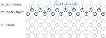
Figure 1: Illustration of a case where a Green’s function method can be used to reduce the number of atoms that need to be included in the simulation; a half-space is partitioned into boundary atoms (dark) and substrate atoms (light); the net force on the latter is zero; the displacement of boundary atoms due to a force field $\vec{f}_{s}(x_{1},x_{2},x_{3}{})$ (coming from substrate atoms and optional explicit atoms) can be calculated without simulating substrate atoms if the Green’s functions ${\mathbf{G}}_{s}$ (which depends on substrate conditions, however) is known; conversely, the force on boundary atoms can be calculated from their displacements if the effective stiffness ${\mathbf{\Phi}}_{s}$ is known.

Let $\vec{f}_{s}(x_{1},x_{2},x_{3}{})$ be the (static) force on the atoms in the boundary region as a function of coordinates $x_{1}$ and $x_{2}$ in the plane, and coordinate $x_{3}$ perpendicular to the plane with positive $x_{3}$ pointing into the substrate. Taking the Fourier transform with respect to the in-plane coordinates yields the representation $\vec{f}_{s}({q_{1}},{q_{2}},x_{3}{})$, with wavenumbers ${q_{1}}$ and ${q_{2}}$. If no external forces act on the substrate atoms, and $\vec{f}_{s}({q_{1}},{q_{2}},x_{3}{})$ were known, then in the static limit the displacements $\vec{u}_{s}({q_{1}},{q_{2}},x_{3}{})$ in the boundary could be calculated using the elastic Green’s function ${\mathbf{G}}_{s}({q_{1}},{q_{2}},x_{3}{})$,

$$\vec{u}_{s}({q_{1}},{q_{2}},x_{3}{})={\mathbf{G}}_{s}({q_{1}},{q_{2}},x_{3}{})\cdot\vec{f}_{s}({q_{1}},{q_{2}},x_{3}{}).$$ (1)

Inversion yields

$$\vec{f}_{s}({q_{1}},{q_{2}},x_{3}{})={\mathbf{\Phi}}_{s}({q_{1}},{q_{2}},x_{3}{})\cdot\vec{u}_{s}({q_{1}},{q_{2}},x_{3}{}),$$ (2)

where ${\mathbf{\Phi}}_{s}={{\mathbf{G}}_{s}}^{-1}$ is a matrix of complex stiffness coefficients, which depends on the substrate configuration. The problem has thus been shifted from simulating substrate atoms to determining ${\mathbf{\Phi}}_{s}$. In the case of unary systems, ${\mathbf{G}}_{s}$ and ${\mathbf{\Phi}}_{s}$ have been measured in molecular dynamics simulations using a fluctuation-dissipation theorem [18, 25], or directly calculated using a transfer matrix or renormalization group approach [20].

The outlined method is limited to homogeneous crystals, since it relies on the assumption that the elastic constants of the medium are invariant under translation. This assumption breaks down in alloys. As a first step towards extending this method for alloys, we examine in this paper the variation of the surface stiffness in a multi-principal element random alloy, where every atom has a random environment. The surface stiffness is the special case of ${\mathbf{\Phi}}_{s}$ where only surface atoms are retained.

We used the Embedded Atom Method (EAM) [26] and calculated ${\mathbf{\Phi}}_{s}$ by inversion of the Hessian matrix $\mathbf{H}$ of the potential energy, the analytical solution of which we have derived for this class of interatomic potentials. We compared the stiffness of the true random alloy to the stiffness of a mean field model of the alloy, where we used the Average-atom (A-atom) [27] approximation. Additionally, we present the anisotropic-elastic solution for ${\mathbf{\Phi}}_{s}$ of a continuous half-space with finite thickness and compare the continuum stiffness to atomistic data.

Our results show that the atomistic solutions converges to the continuum in the limit of long wavelengths. At short wavelengths, the local environment of atoms controls ${\mathbf{\Phi}}_{s}$, hence the continuum solution is a poor estimate. The average alloy model is a fair approximation for the mean stiffness of the true random alloy at all wavelengths, but fluctuations grow substantially as the wavelength decreases.

II Methods

II.1 Atomistic stiffness

We calculated the stiffnesses of the (001) surface of face-centered cubic (FCC) crystals using square slab configurations, see Fig. 2. The simulation cell was a rectangular prism with a square base. Consider a Cartesian coordinate system with directions $x_{1}$ and $x_{2}$ in the plane of the base. In order to simulate a half-space, we applied periodic boundary conditions along the $x_{1}$- and $x_{2}$-directions, and open boundary conditions along the $x_{3}$-direction. The lattice directions [110], [1-10], and [001] of the crystal were parallel to the $x_{1}$-, $x_{2}$-, and $x_{3}$-directions of the cell.

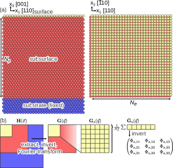
Figure 2: (a) Configuration used for calculating the surface stiffness ${\mathbf{\Phi}}_{s}$ in side view (left) and top view (right). Atoms in the substrate layers (blue, thickness two times the potential cutoff radius) were fixed in positions corresponding to static equilibrium under fully periodic boundary conditions. Atoms in the subsurface (red) and surface (yellow) layers were free. Periodic boundary conditions were applied in the $x_{1}$- and $x_{2}$-directions. The $\hkl(001)$ planes (perpendicular to the $x_{3}$-direction) are square lattices with $N_{e}$ atoms along the edges; the subsurface region consists of $N_{p}$ $\hkl(001)$ planes. (b) Illustration of the calculation of ${\mathbf{\Phi}}_{s}$; the upper left block of the Hessian matrix $\mathbf{H}$ (left) involves only surface and subsurface atoms; this block is inverted and Fourier-transformed to obtain Green’s functions $\mathbf{G}$ (middle); the upper left $3N_{e}\times{}3N_{e}$ sub-block corresponding to interactions between surface atoms contains the surface Green’s functions ${\mathbf{G}}_{s}$; each of the $N_{e}^{2}$ $3\times 3$ blocks contains the values of Green’s functions for one pair of atoms $\nu\mu$, i.e. one wavevector $({q_{1}},{q_{2}})$ in the plane; one row of blocks corresponds to the Green’s functions with one site $\nu$ fixed; the surface stiffness matrices ${\mathbf{\Phi}}_{s}$ are the harmonic averages obtained by first averaging block rows of ${\mathbf{G}}_{s}$ and then calculating the matrix inverse of each block

The set of (001) planes can be partitioned into surface, subsurface, and substrate planes. There is only one surface plane, but $N_{p}$ subsurface and $N_{u}$ substrate planes. We call the corresponding sets of atoms $\Omega_{s}$, $\Omega_{p}$ and $\Omega_{u}$. Atoms in (001) planes form a 2D square lattice with lattice parameter $a=a_{0}/\sqrt{2}$, where $a_{0}$ is the FCC lattice parameter. Let there be $N_{e}$ atoms along the edge in the $x_{1}$- or $x_{2}$-direction, then there are $N_{e}^{2}$ atoms in each plane, and the total number of atoms is $N=(1+N_{p}+N_{s})N_{e}^{2}$. In order to eliminate surface effects at the bottom boundary, we fixed the substrate atoms in positions corresponding to static equilibrium under fully periodic boundary conditions and made the fixed substrate layer thicker than the maximum interaction distance of the potential. We used Embedded Atom Method (EAM) [26] potentials, hence the required thickness was two times the cutoff radius $r_{\textrm{cut}}$ of the potential. The process of constructing the configurations depends on the material and is explained in detail below.

To determine the surface stiffnesses ${\mathbf{\Phi}}_{s}$, we first calculated the Green’s functions $\mathbf{G}$ by inverting the Hessian matrix $\mathbf{H}$ of the potential energy $\mathcal{V}^{\mathrm{int}}$, see Fig. 2 (b). The components of $\mathbf{H}$ are

$$H_{(3(\nu{}-1)+i)(3(\mu{}-1)+j)}=\frac{\partial^{2}\mathcal{V}^{\mathrm{int}}\left(\left\{\vec{x}\right\}\right)}{\partial x_{i}^{(\nu)}\partial x_{j}^{(\mu)}}\bigg{|}_{\left\{\vec{x}\right\}_{0}},$$ (3)

where indices $\mu,\nu\in[1,N]$ refer to atoms, and indices $i,j\in[1,2,3]$ refer to the three components of a vector in $x_{1}$-, $x_{2}$- and $x_{3}$-direction. In this equation $\left\{\vec{x}\right\}$ is the set of position vectors of the atoms $\left\{\vec{x}\right\}\equiv\left\{{\vec{x}}^{(1)},\dots,{\vec{x}}^{(N)}\right\}$, and $x_{i}^{(\nu)}$ is the coordinate of atom $\nu$ in $i$-direction. $\left\{\vec{x}\right\}_{0}$ is the set of equilibrium positions where the force on the atoms vanishes. We used the analytical solution of $\mathbf{H}$ for EAM potentials, see the derivation in Appendix B. This solution is implemented in the Python package matscipy [28].

$\mathbf{H}$ is a real symmetric $3N\times{}3N$ matrix. It is sparse, because the range of interaction between atoms is limited. Consider an arbitrary displacement of the atoms, written as a $3N$-dimensional vector $\vec{u}$. Within the harmonic approximation, the components of the resulting force vector $\vec{f}$ are

$$f_{3(\nu-1)+i}=H_{((3\nu-1)+i)(3(\mu-1)+j)}u_{3(\mu-1)+j},$$ (4)

where repeated indices imply summation over the corresponding range. Recall that the atoms in $\Omega_{u}$ are fixed in their equilibrium positions, hence $u$ vanishes for those atoms. To impose this constraint, we computed $\mathbf{H}$ of the whole configuration, but then eliminated elements in $\mathbf{H}$ corresponding to pairs of atoms where one or both of them are in $\Omega_{u}$. The remaining $3(1+N_{p})N_{e}\times 3(1+N_{p})N_{e}$ elements correspond to pairs of atoms in $\Omega_{s}\cup\Omega_{p}$. It is convenient to label the atoms such that these elements form the upper left block of $\mathbf{H}$ (see Fig. 2b).

This block was then inverted to obtain Green’s functions $G_{(3(\nu-1)+i)(3(\mu-1)+j)}$, which solve

$$u_{3(\nu-1)+i}=G_{(3(\nu-1)+i)(3(\mu-1)+j)}f_{3(\mu-1)+j},$$ (5)

where $\nu,\mu\in{}\Omega_{s}\cup\Omega_{p}$. To bring out the block structure of $G_{3(\nu-1)+i)(3(\mu-1)+j)}$, we can rewrite this equation as

$$\vec{u}^{(\nu)}=\sum_{\mu\in{}\Omega_{s}\cup\Omega_{p}}\mathbf{G}^{(\nu,\mu)}\cdot\vec{f}^{(\mu)},$$ (6)

where $\vec{u}^{(\nu)}$ is the displacement vector of atom $\nu$, with components $u_{3(\nu-1)+i}$ ($i=1,2,3$) in Eq. (5); $\mathbf{G}^{(\nu,\mu)}$ is the $3\times{}3$ block $G_{(3(\nu-1)+i)(3(\mu-1)+j)}$; and $\vec{f}^{(\mu)}$ corresponds to the components $f_{3(\mu-1)+i}$ ($i=1,2,3$).

We inverted $\mathbf{H}$ via Cholesky factorization, using petsc [29, 30] and mumps [31, 32]. The latter allows parallel calculation of the selected entries [33] in the upper left block of the matrix. For pure crystals, the surface Green’s function can be computed efficiently using renormalization group approaches for system sizes beyond billions of atoms [20].

Using the same argument to eliminate the substrate atoms from $\mathbf{H}$, we now eliminate the subsurface atoms from $\mathbf{G}$: the forces on the subsurface atoms must vanish since we are working in the static limit – which means that all subsurface atoms remain in their equilibrium positions. The remaining quantity is a $3N_{s}\times{}3N_{s}$ matrix ${\mathbf{G}}_{s}$ describing the degrees of freedom corresponding to the surface atoms. Eq. (6) (with $\nu,\mu\in\Omega_{s}$) can be interpreted as a signal measured at $3N_{s}\times{}3N_{s}$ points $\{(x_{1}^{(\nu)},x_{2}^{(\nu)})\mid{}\nu\in\Omega_{s}\}$ in the plane, and we write

$$\vec{u}_{s}(x_{1}^{(\nu)},x_{2}^{(\nu)})=\sum_{\mu\in{}\Omega_{s}}{\mathbf{G}}_{s}(x_{1}^{(\nu)},x_{2}^{(\nu)},x_{1}^{(\mu)},x_{2}^{(\mu)})\cdot\vec{f}_{s}(x_{1}^{(\mu)},x_{2}^{(\mu{})}).$$ (7)

In a pure crystal with translational symmetry in the plane, Green’s functions would only depend on the relative distance between points, i.e. ${\mathbf{G}}_{s}(x_{1}^{(\nu)},x_{2}^{(\nu)},x_{1}^{(\mu)},x_{2}^{(\mu)})\rightarrow{\mathbf{G}}_{s}(x_{1}^{(\nu)}-x_{1}^{(\mu)},x_{2}^{(\nu)}-x_{2}^{(\mu)})$, and Eq. (7) would be a convolution. According to the convolution theorem, taking the discrete Fourier transform of Eq. (7) would then produce Eq. (2).

However, in random alloys translational symmetry is broken. Thus, we studied the variation of stiffness across sites. We denote the Green’s functions of site $\nu$ as

$${\mathbf{G}}_{s}^{(\nu)}(x_{1}^{(\nu)}-x_{1}^{(\mu)},x_{2}^{(\nu)}-x_{2}^{(\mu)})\equiv{}{\mathbf{G}}_{s}(x_{1}^{(\nu)},x_{2}^{(\nu)},x_{1}^{(\mu)},x_{2}^{(\mu)})$$ (8)

in what follows. Note that in Eq. (8) the argument of ${\mathbf{G}}_{s}^{(\nu)}$ is measured with respect to the position of the site $\vec{x}^{(\nu)}$ such that we can carry out a Fourier-transform for each site. This representation is useful for comparison with the unary system and the continuum solution, where the per-site variation disappears from Eq. (8). Neglecting non-affine microdistortions [34, 35, 36], the atoms are arranged approximately in a simple cubic lattice within the periodic domain. Hence in equilibrium

$$\begin{split}(x_{1}^{(\nu)}-x_{1}^{(\mu)},x_{2}^{(\nu)}-x_{2}^{(\mu)})&\approx(ma,na),\\ &\text{with}\;m,n\in\left\{0,\dots,N_{e}-1\right\}.\end{split}$$ (9)

The discrete Fourier transform of ${\mathbf{G}}_{s}^{(\nu)}\left(ma,na\right)$ is

$$\begin{aligned} {\mathbf{G}}_{s}^{(\nu)}\left(\frac{2\pi}{aN_{e}}k,\frac{2\pi}{aN_{e}}l\right)=&\sum_{m}^{N_{e}-1}\sum_{n}^{N_{e}-1}{\mathbf{G}}_{s}^{(\nu)}\left(ma,na\right)\exp\left\{-2\pi{}i\left(\frac{mk}{N_{e}}+\frac{ml}{N_{e}}\right)\right\},\;\text{with}\;k,l\in\left\{0,\dots,N_{e}-1\right\}\end{aligned}$$ (10)

. Thus, we map the solution to $N_{e}\times{}N_{e}$ wavevectors in the first Brillouin zone with components

$${q_{1}},{q_{2}}\in\begin{dcases}\left\{-\frac{N_{e}}{2},\dots,\frac{N_{e}}{2}-1\right\}\cdot\frac{2\pi}{aN_{e}}&\,\text{$N_{e}$ even}\\ \left\{-\frac{N_{e}-1}{2},\dots,\frac{N_{e}-1}{2}\right\}\cdot\frac{2\pi}{aN_{e}}&\,\text{$N_{e}$ odd}\end{dcases}.$$ (11)

However, due to symmetry only the quadrant $0\leq{}{q_{1}},{q_{2}}\leq{\pi/a}$ is unique.

In an unary system, ${\mathbf{G}}_{s}^{(\nu)}({q_{1}},{q_{2}})$ is the same for all sites $\nu$. In a random alloy, on the other hand, there are site-by-site variations, and the components $G_{s,ij}^{(\nu)}({q_{1}},{q_{2}})$ of ${\mathbf{G}}_{s}^{(\nu)}({q_{1}},{q_{2}})$ become complex random variables.

Rather than discussing the surface Greens function itself ${\mathbf{G}}_{s}(\vec{q})$, it is convenient to discuss its inverse, the surface stiffness ${\mathbf{\Phi}}_{s}(\vec{q})$. This is because in the long-wavelength (continuum) limit ${\mathbf{\Phi}}_{s}(\vec{q})\propto q$ [10, 18, 20] while ${\mathbf{G}}_{s}(\vec{q})$ diverges. The question we will discuss in the following is how to characterize the mean response of the solid and the magnitude of per-site fluctuations.

We first computed a mean stiffness ${\mathbf{\Phi}}_{s}({q_{1}},{q_{2}})$. Consider the related problem of stochastic homogenization of an elastic continuum with fluctuating elastic constants. Here, the effective stiffness of the homogenized medium can be computed using the solution of a corrector equation [37, 38]. The solutions of the equation with random coefficients then converge to the solution of the homogenized equation in mean. Let

$${\mathbf{\Phi}}_{s}^{(\nu)}({q_{1}},{q_{2}})\equiv\left({\mathbf{G}}_{s}^{(\nu)}({q_{1}},{q_{2}})\right)^{-1}$$ (12)

be the stiffness of site $\nu$. Following the continuum approach, we computed the average surface stiffness as

$$\begin{aligned} {\mathbf{\Phi}}_{s}({q_{1}},{q_{2}})=\left\langle\left({\mathbf{\Phi}}_{s}^{(\nu)}({q_{1}},{q_{2}})\right)^{-1}\right\rangle^{-1}={\bar{\mathbf{G}}_{s}}^{-1}\left({q_{1}},{q_{2}}\right),\end{aligned}$$ (13)

where $\left\langle\dots\right\rangle$ indicates the arithmetic mean over all sites, i.e. the components of ${\bar{\mathbf{G}}_{s}}\left({q_{1}},{q_{2}}\right)$ are

$$\bar{G}_{s,ij}({q_{1}},{q_{2}})=\frac{1}{N_{e}^{2}}\sum_{\nu=1}^{N_{e}^{2}}G_{s,ij}^{(\nu)}({q_{1}},{q_{2}}).$$ (14)

We calculated ${\mathbf{\Phi}}_{s}({q_{1}},{q_{2}})$ of pure Ni, and ${\mathbf{\Phi}}_{s}({q_{1}},{q_{2}})$ of a random solid solution of Fe, Ni and Cr with equal concentration of all elements. In both cases, we used the EAM potential by Bonny et al. [39], which has a smooth cutoff with continuous first and second derivatives. We prepared the random Fe-Ni-Cr alloy by randomly assigning the constituent elements to the lattice sites. Additionally, we performed calculations with a mean-field model. Here, we replaced the different real elements by a single “average” element, the A-atom [40, 27]. It behaves like a pure metal with similar average properties as the true random solution. A module for generating A-atom potentials has been implemented in the Python package matscipy [28]. In pure Ni and the A-atom crystal, ${\mathbf{\Phi}}_{s}^{(\nu)}({q_{1}},{q_{2}})$ is the same for all surface sites $\nu$, hence ${\mathbf{\Phi}}_{s}({q_{1}},{q_{2}})={\mathbf{\Phi}}_{s}^{(\nu)}({q_{1}},{q_{2}})$. The harmonic mean of the random alloy data according to Eq. (13) can be compared to the A-atom solution and the continuum solution. The latter requires only three cubic elastic constants as input.

In the case of the Ni and A-atom configurations, our starting point was a perfect crystal lattice with the appropriate $0\text{\,}\mathrm{K}\text{/}$ lattice parameter. We then minimized the potential energy of the surface and subsurface atoms using fire [41, 42]. The substrate atoms were fixed during minimization and the iteration was stopped as soon as the Euclidean norm of the global force vector fell below $1\text{\times}{10}^{-6}\text{\,}\mathrm{eV}\text{/}\mathrm{\SIUnitSymbolAngstrom}$. In order to create the random FeNiCr alloy, we started from a thicker, fully periodic configuration. We added an additional slab of atoms of thickness greater than $2r_{\textrm{cut}}$ below the substrate and then minimized the potential energy under fully periodic boundary conditions. This minimization allowed the substrate atoms to move to their non-affine equilibrium positions in the bulk. Afterwards, we opened the boundary along the $x_{3}$-direction and removed the extra atoms. Finally, we minimized the potential energy of the open system with fixed substrate atoms.

The required lattice parameters and elastic constants of the three materials are listed in Tab. 1 in Appendix A. See this appendix also for details on how the values were computed.

II.2 Continuum stiffness

We consider a semi-infinite solid, see Fig. 3. The body has a surface perpendicular to the $x_{3}$-direction and extends to infinity in the $x_{1}$- and $x_{2}$- directions. Positive $x_{3}$ are located within the solid. In the $x_{3}$-direction, the body may have a finite thickness $h$, or infinite thickness $h\rightarrow\infty$. We discuss both cases. Tractions $\vec{Q}(x_{1},x_{2})$ are applied at the surface and there are no body forces. In the case where the body has finite thickness $h$, we assume a fixed boundary, i.e. $\vec{u}(x_{1},x_{2},h)=0$. The material is homogeneous and linear-elastic, with anisotropic elastic constants $C_{ijkl}$ ($i,j,k,l\in[1,2,3]$) subject to the usual symmetry requirements [43]. For the FCC solid considered here, there are three indendent elastic constant that are typically denoted by $C_{11}$, $C_{12}$ and $C_{44}$.

We are interested in the surface displacements $\vec{u}_{s}(x_{1},x_{2})$ in elastostatic equilibrium, where the divergence of the stress tensor $\sigma$ vanishes,

$$\partial_{i}\sigma_{ij}=0.$$ (15)

$\partial_{i}$ indicates the partial derivative in direction $i$ and Einstein summation convention applies. Eq. (15) corresponds to requiring zero forces for the subsurface atoms in our atomistic calculations.

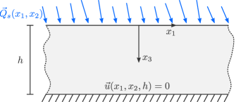
Figure 3: Model used for deriving a continuum solution of the surface Green function and the associated stiffness tensor; the surface at $x_{3}=0$ is subjected to tractions $\vec{Q}_{s}(x_{1},x_{2})$; we consider finite thickness $h$ with fixed boundary conditions at $x_{3}=h$, and the limit $h\rightarrow\infty$; the solid is infinite along $x_{1}$ and $x_{2}$; the material has anisotropic elastic constants $C_{ijkl}$, which are constant throughout the body

$\vec{u}_{s}(x_{1},x_{2})$ can be calculated by a convolution of the tractions $\vec{Q}(x_{1},x_{2})$ with surface Green’s function ${\mathbf{G}}_{s}(x_{1},x_{2})$,

$$\vec{u}_{s}(x_{1},x_{2})=\int dx_{1}^{\prime}dx_{2}^{\prime}{\mathbf{G}}_{s}(x_{1}-x_{1}^{\prime},x_{2}-x_{2}^{\prime})\cdot\vec{Q}(x_{1}^{\prime},x_{2}^{\prime}).$$ (16)

Fourier transformation yields Eq. (1) (with $x_{3}=0$ dropped). In Appendix C, we derive ${\mathbf{G}}_{s}({q_{1}},{q_{2}})$ for finite $h$ and $h\rightarrow\infty$. The solution can be represented as a matrix product

$${\mathbf{G}}_{s}({q_{1}},{q_{2}})=\mathbf{U}({q_{1}},{q_{2}},0)\cdot\mathbf{F}^{-1}({q_{1}},{q_{2}}).$$ (17)

The matrices $\mathbf{U}({q_{1}},{q_{2}},0)$ and $\mathbf{F}({q_{1}},{q_{2}})$ depend on the eigenvalues of the Fourier transform of the linear operator

$$M_{il}=C_{ijkl}\partial_{j}\partial_{k},$$ (18)

and the admissible basis functions of the displacement field. No closed-form solution exists, but it is straightforward to calculate said eigenvalues and basis functions numerically. The inverse of ${\mathbf{G}}_{s}({q_{1}},{q_{2}})$ is the surface stiffness ${\mathbf{\Phi}}_{s}({q_{1}},{q_{2}})$. We have implemented the numerical solution of ${\mathbf{\Phi}}_{s}({q_{1}},{q_{2}})$ in the Python package ContactMechanics [44].

III Results

We first calculated the surface stiffness of Ni to obtain reference data for a pure metal. The atomic configuration had $N_{e}=31$ atoms along the edge, and $N_{p}=45$ subsurface planes. All $N_{e}^{2}=961$ solutions of ${\mathbf{\Phi}}_{s}^{(\nu)}$ for different surface sites $\nu$ are equal due to translational symmetry in the plane. Notice that $\vec{f}_{s}^{(\nu)}$ in Eq. (7) of the atomistic solution is a force, whereas $\vec{Q}$ in Eq. (16) of the continuum solution is a traction (units of $\text{\,}\mathrm{N}\text{/}{\mathrm{m}}^{2}$). In order to compare atomistic and continuum Green’s functions, we need to divide the former by the mean area per atom $a^{2}=a_{0}^{2}/2$. The resulting Green’s function has SI units of $\text{\,}\mathrm{N}\text{/}{\mathrm{m}}^{3}$, but it is more convenient to use $\text{\,}\mathrm{GPa}\text{/}\mathrm{\SIUnitSymbolAngstrom}$, since $\Phi_{s,11}$, for example, should converge to $C_{44}/h$ in the limit of infinite wavelength.

Figure 4 shows $\Re\Phi_{s,33}({q_{1}},{q_{2}})$ in the quadrant of the surface Brillouin zone where $0\leq{}{q_{1}},{q_{2}}\leq{\pi/a}$. Here and in the following, $\Re$ and $\Im$ refer to the real and imaginary parts of an imaginary number, respectively. The other quadrants are symmetric with respect to the ${q_{1}}$- and ${q_{2}}$-axes. The stiffness is minimal in the long-wavelength limit ${q_{1}}={q_{2}}=0$ and increases with decreasing wavelength. The origin ${q_{1}}={q_{2}}=0$ is called $\bar{\Gamma}$. The center of the edge of the Brillouin zone along ${q_{1}}$ is called $\bar{X}$, and the corner is called $\bar{M}$. Below, we show plots of values along the path $\bar{\Gamma}$-$\bar{X}$-$\bar{M}$-$\bar{\Gamma}$. To study convergence in the long-wavelength limit, we also consider a shorter path $\bar{\Gamma}$-$\bar{X}^{\prime}$-$\bar{M}^{\prime}$-$\bar{\Gamma}$, where $\bar{X}^{\prime}$ is on the line ${q_{2}}=0$, at $10\text{\,}\mathrm{\char 37\relax}\text{/}$ of the distance from $\bar{\Gamma}$ to $\bar{X}$. Point $\bar{M}^{\prime}$ corresponds to a wavelength of $11\text{\,}\mathrm{\SIUnitSymbolAngstrom}\text{/}$ along the $x_{1}$- and $x_{2}$-directions.

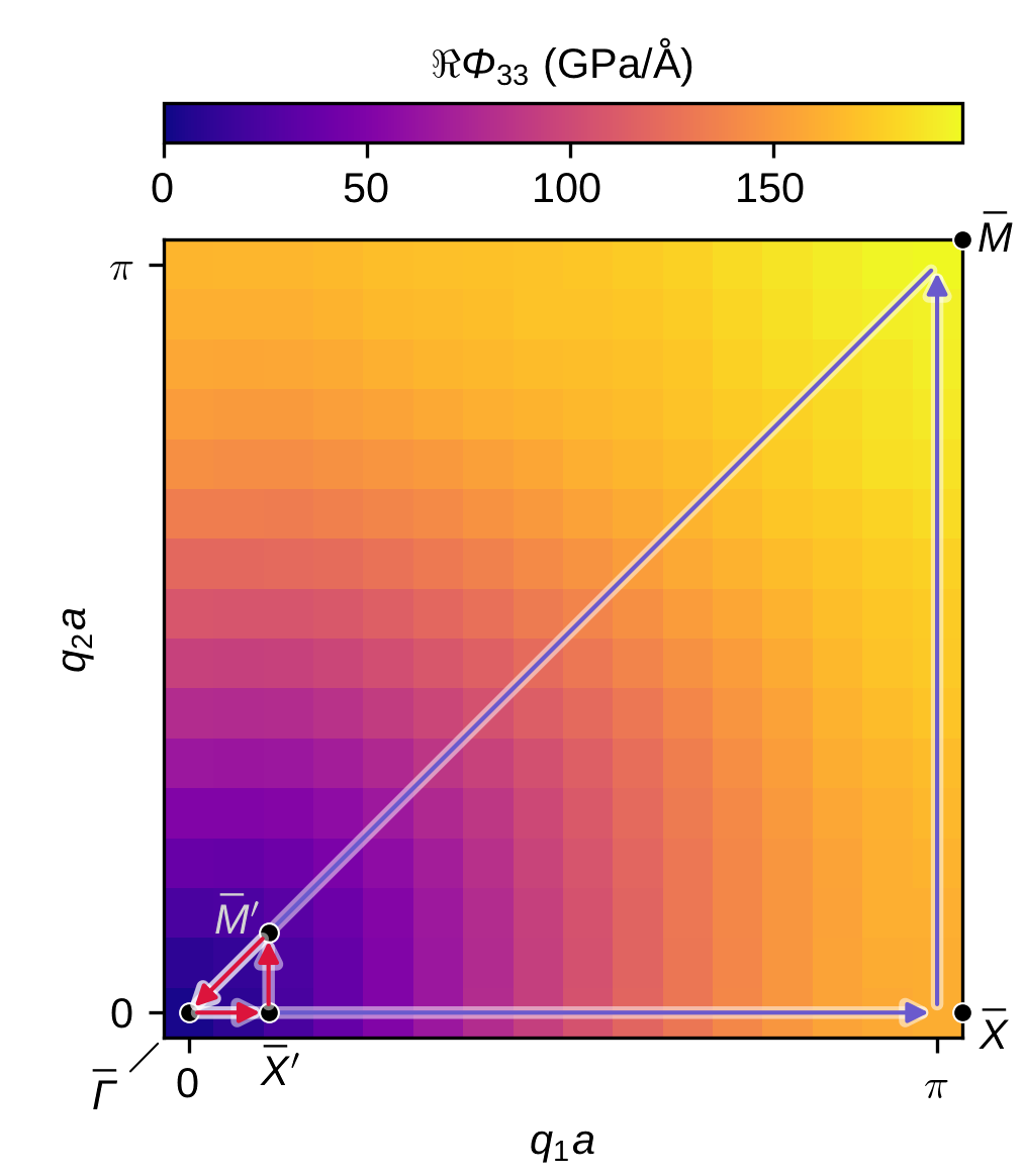
Figure 4: Real part of stiffness component $\Phi_{s,33}$ of Ni in a quadrant of the surface Brillouin zone; in other figures we have plotted the values along the paths $\bar{\Gamma}$-$\bar{X}$-$\bar{M}$-$\bar{\Gamma}$ and $\bar{\Gamma}$-$\bar{X}^{\prime}$-$\bar{M}^{\prime}$-$\bar{\Gamma}$.

The upper two rows of Fig. 5 show the six independent components of ${\mathbf{\Phi}}_{s}$ along the path $\bar{\Gamma}$-$\bar{X}$-$\bar{M}$-$\bar{\Gamma}$. Four moduli are purely real, namely the normal moduli $\Phi_{s,11}$, $\Phi_{s,22}$, and $\Phi_{s,33}$, as well as the in-plane shear modulus $\Phi_{s,12}$. The out-of-plane shear moduli $\Phi_{s,23}$ and $\Phi_{s,13}$ are purely imaginary. The discrepancy between the continuum data and the atomistic data increases as one moves away from the long-wavelength limit near $\bar{\Gamma}$ towards $\bar{X}$ or $\bar{M}$. The difference is maximum at corner of the surface Brillouin zone $\bar{M}$, which represents the short-wavelength limit in both in-plane directions. In the case of the shear moduli, the continuum model fails to predict the extrema between $\bar{X}$ and $\bar{M}$ (zone edge), and between $\bar{M}$ and $\bar{\Gamma}$ (zone diagonal). The bottom row of Fig. 5 shows the components $\Phi_{s,11}$, $\Phi_{s,22}$, and $\Phi_{s,12}$ along the path $\bar{\Gamma}$-$\bar{X}^{\prime}$-$\bar{M}^{\prime}$-$\bar{\Gamma}$. These plots indicate that the continuum and atomistic solutions converge near $\bar{\Gamma}$. The solutions for $\Phi_{s,12}$ agree qualitatively. The atomistic value of $\Phi_{s,11}$ and $\Phi_{s,22}$ at $\bar{\Gamma}$ is $1.6\text{\,}\mathrm{GPa}\text{/}\mathrm{\SIUnitSymbolAngstrom}$, which is equal to $C_{44}/h$ with $C_{44}=$125\text{\,}\mathrm{GPa}\text{/}$$ and $h=45a_{0}/2=$79.2\text{\,}\mathrm{\SIUnitSymbolAngstrom}\text{/}$$.

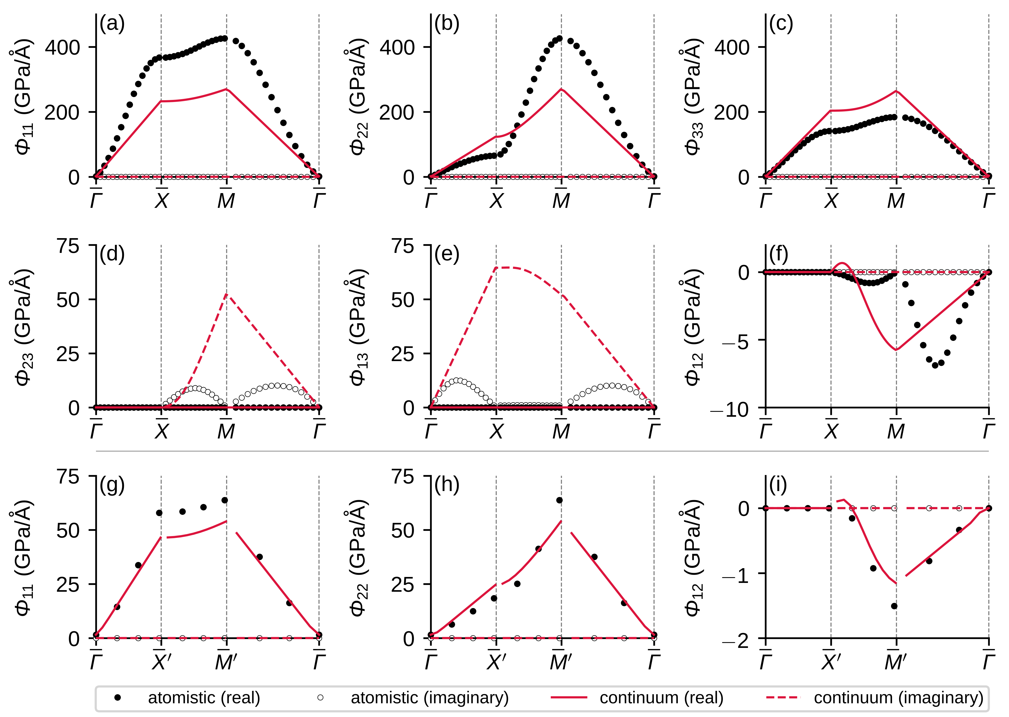
Figure 5: Surface stiffness of Ni; markers: atomistic model; lines: anisotropic-elastic model; the upper two rows show the variation of the six independent components along the path $\bar{\Gamma}$-$\bar{X}$-$\bar{M}$-$\bar{\Gamma}$ through the first quadrant of the surface Brillouin zone (see Fig. 4); the normal moduli $\Phi_{s,11}$, $\Phi_{s,22}$, and $\Phi_{s,33}$, as well as the shear modulus $\Phi_{s,12}$ are purely real; the two in-plane shear moduli $\Phi_{s,23}$ and $\Phi_{s,13}$ are purely imaginary; atomistic and continuum models disagree near points $\bar{X}$ and $\bar{M}$, which are short wavelength limits; the lower row shows the values of $\Phi_{s,11}$, $\Phi_{s,22}$, and $\Phi_{s,12}$ along the shorter path $\bar{\Gamma}$-$\bar{X}^{\prime}$-$\bar{M}^{\prime}$-$\bar{\Gamma}$ through the long wavelength region; the relative difference between atomistic and continuum models decreases with increasing wavelength

Having examined the surface stiffness of pure Ni, we now attend to the alloy case. We created $500$ random alloy samples and one average alloy sample with $N_{p}=45$ and $N_{e}=31$. Below, we report the arithmetic mean of $\Phi_{s,ij}({q_{1}},{q_{2}})$ of all random alloy samples. However, sample-by-sample variations of $\Phi_{s,ij}({q_{1}},{q_{2}})$ are small, since this is the homogenized stiffness with fluctuations averaged out. Additionally, we quantified site-by-site fluctuations by calculating the 10th and 90th percentiles of the site-specific stiffness tensors ${\mathbf{\Phi}}_{s}^{(\nu)}({q_{1}},{q_{2}})$ at all sites in all samples, i.e. $500\cdot{}N_{e}^{2}=480500$ sites in total.

Fig. 6 shows the stiffness components along the paths $\bar{\Gamma}$-$\bar{X}$-$\bar{M}$-$\bar{\Gamma}$ and $\bar{\Gamma}$-$\bar{X}^{\prime}$-$\bar{M}^{\prime}$-$\bar{\Gamma}$. The upper two rows show the real parts of $\Phi_{s,11}$, $\Phi_{s,22}$, $\Phi_{s,33}$, $\Phi_{s,12}$, as well as the imaginary parts of $\Phi_{s,13}$ and $\Phi_{s,23}$ along $\bar{\Gamma}$-$\bar{X}$-$\bar{M}$-$\bar{\Gamma}$. The bottom row shows $\Re\Phi_{s,11}$, $\Re\Phi_{s,22}$, and $\Re\Phi_{s,12}$ along the long-wavelength path $\bar{\Gamma}$-$\bar{X}^{\prime}$-$\bar{M}^{\prime}$-$\bar{\Gamma}$. The average alloy behaves like a pure metal, hence ${\mathbf{G}}_{s}\left({q_{1}},{q_{2}}\right)$ is the same for all surface sites, and there is one unique $3\times{}3$ stiffness matrix ${\mathbf{\Phi}}_{s}\left({q_{1}},{q_{2}}\right)$ for every point $\left({q_{1}},{q_{2}}\right)$ in the Brillouin zone. In the random alloy, by contrast, ${\mathbf{G}}_{s}\left({q_{1}},{q_{2}}\right)$ fluctuates, therefore a different stiffness ${\mathbf{\Phi}}_{s}\left({q_{1}},{q_{2}}\right)$ would be obtained for a different element distribution. In Fig. 6, markers indicate the harmonic mean ${\mathbf{\Phi}}_{s}\left({q_{1}},{q_{2}}\right)$, and shaded areas the 10th and 90th percentiles of the site stiffnesses ${\mathbf{\Phi}}_{s}^{(\nu)}\left({q_{1}},{q_{2}}\right)$. Sample-by-sample variations of ${\mathbf{\Phi}}_{s}\left({q_{1}},{q_{2}}\right)$ are negligible. The difference between the corresponding 10th and 90th percentiles is less than the size of the markers of ${\mathbf{\Phi}}_{s}\left({q_{1}},{q_{2}}\right)$ in the plot.

${\mathbf{\Phi}}_{s}\left({q_{1}},{q_{2}}\right)$ should be compared to the corresponding average alloy data and the continuum solution. All three models yield similar results in the long-wavelength limit. For example, the mean value of $\Re\Phi_{s,11}$ and $\Re\Phi_{s,22}$ at $\bar{\Gamma}$ is $1.70\text{\,}\mathrm{GPa}\text{/}\mathrm{\SIUnitSymbolAngstrom}$. The average-alloy value is $1.74\text{\,}\mathrm{GPa}\text{/}\mathrm{\SIUnitSymbolAngstrom}$ and the continuum solution is $1.70\text{\,}\mathrm{GPa}\text{/}\mathrm{\SIUnitSymbolAngstrom}$. The continuum solution fails at short wavelengths, as was observed already in the Ni example. However, the average alloy data remain comparatively close to the mean values of the random alloy. For example, the relative difference between $\Re\Phi_{s,11}$ of the average and random alloy varies between $3\text{\,}\mathrm{\char 37\relax}\text{/}$ and $4\text{\,}\mathrm{\char 37\relax}\text{/}$ along the path. The continuum solution, on the other hand, underestimates the mean along most of the path, except near $\bar{\Gamma}$. Near $\bar{X}$, the continuum value is $33\text{\,}\mathrm{\char 37\relax}\text{/}$ lower than the mean value of the random alloy. The absolute value of the relative difference between $\Re\Phi_{s,22}$ of the average and random alloy varies between $3\text{\,}\mathrm{\char 37\relax}\text{/}$ and $11\text{\,}\mathrm{\char 37\relax}\text{/}$. In the case of $\Re\Phi_{s,33}$, the absolute relative difference does not exceed $4\text{\,}\mathrm{\char 37\relax}\text{/}$. Recall that the continuum solution for $\Re\Phi_{s,12}$ of pure Ni was qualitatively different from the atomistic solution. The same is true for the alloy. The continuum solution has a local minimum at $\bar{M}$, whereas both atomistic solutions have their minimum between $\bar{M}$ and $\bar{\Gamma}$.

Fluctuations in the random alloy data are close to zero at $\bar{\Gamma}$, but increase with decreasing wavelength. For example, the relative difference between the 90th percentile of the site-specific values of $\Re\Phi_{s,11}$ and the mean according to Eq. (13) increases from less than $1\text{\,}\mathrm{\char 37\relax}\text{/}$ of the mean value at $\bar{\Gamma}$ to $70\text{\,}\mathrm{\char 37\relax}\text{/}$ at $\bar{X}$. Interestingly, it decreases to $38\text{\,}\mathrm{\char 37\relax}\text{/}$ at $\bar{M}$, even though $\bar{M}$ represents the limit of short wavelengths in both in-plane directions. The maximum fluctuations of $\Re\Phi_{s,33}$ are smaller than those of $\Re\Phi_{s,11}$ and $\Re\Phi_{s,22}$.

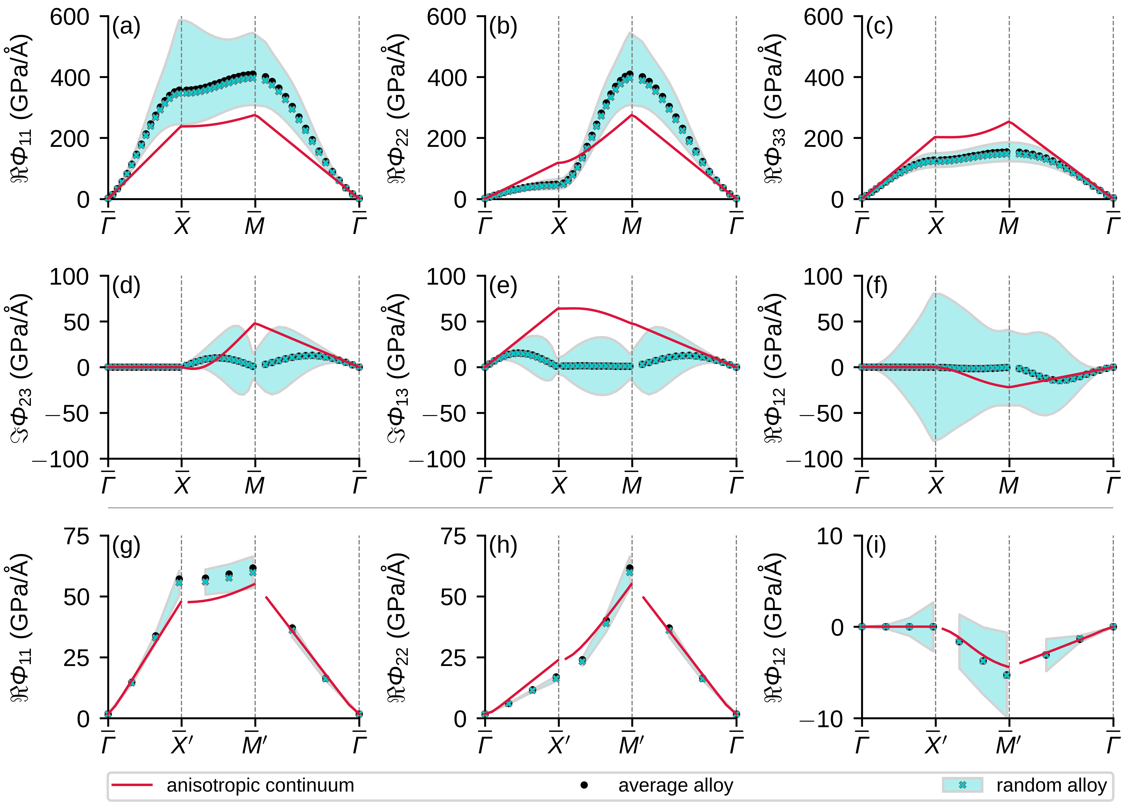
Figure 6: Surface stiffness of an equicomposition FeNiCr alloy; the upper two rows show the real parts of $\Phi_{s,11}$, $\Phi_{s,22}$, $\Phi_{s,33}$, $\Phi_{s,12}$, as well as the imaginary parts of $\Phi_{s,13}$ and $\Phi_{s,23}$ along the path $\bar{\Gamma}$-$\bar{X}$-$\bar{M}$-$\bar{\Gamma}$ through the first quadrant of the surface Brillouin zone (see Fig. 4); the stiffness of the average alloy is close to the effective mean stiffness of the true random alloy according to Eq. (13); turquoise areas indicate the range between the 10th and 90th percentile of the distribution of site stiffnesses; stiffness fluctuations are small at long wavelengths; with the exception of $\Phi_{s,33}$, fluctuations grow significantly at short wavelengths; the lower row shows the values of $\Phi_{s,11}$, $\Phi_{s,22}$, and $\Phi_{s,12}$ along the path $\bar{\Gamma}$-$\bar{X}^{\prime}$-$\bar{M}^{\prime}$-$\bar{\Gamma}$ through the long wavelength region; fluctuations in the random alloy, and the relative discrepancy between the atomistic data and the anisotropic-elastic model (red line) are smaller than at short wavelengths

Fig. 7 gives a more detailed view of convergence in the long wavelength limit, using the example of $\Re\Phi_{s,11}$. Fig. 7 (a) shows the ratio between the real values of the atomistic and continuum data along the diagonal $\bar{\Gamma}$-$\bar{M}$. At $\bar{\Gamma}$, the relative error between random alloy and continuum is below $1\text{\,}\mathrm{\char 37\relax}\text{/}$. The average alloy stiffness is $2\text{\,}\mathrm{\char 37\relax}\text{/}$ higher than the continuum value. The second point corresponds to the largest finite wavelength $(31a,31a)$. Here, both atomistic systems are softer than the continuum. At wavelengths shorter than $(15.5a,15.5a)$, the atomistic systems are stiffer than the continuum. Fig. 7 (b) distinguishes between contributions from different elements. Let $\Omega_{\mathrm{Fe}}$ be the set of sites occupied by Fe atoms. To generate the corresponding curve in Fig. 7 (b), the average in Eq. (14) was restricted to sites $\nu\in\Omega_{\mathrm{Fe}}$. Similarly, the 10th and 90th percentiles of ${\mathbf{\Phi}}_{s}^{(\nu)}({q_{1}},{q_{2}})$ were computed only for this subset. The calculation for the other elements is analogous. All three mean values converge in the limit of long wavelengths to the mean stiffness across all sites, and all fluctuations become minimal. Finally, in Fig. 7 (c) we examined the growth of the dispersion of $\Re\Phi_{s,11}^{(\nu)}$ along $\bar{\Gamma}$-$\bar{M}$. The figure shows the difference between the 90th and 10th percentile of $\Re\Phi_{s,11}^{(\nu)}$, divided by the harmonic mean. Between $\bar{\Gamma}$ and $q_{x}a=q_{y}a=1.22$ (corresponding to a wavelength of $\lambda_{x}=\lambda_{y}\approx{}5a$), the ratio grows approximately linearly. A linear least-squares fit yields a slope of $0.47\text{\,}\mathrm{\SIUnitSymbolAngstrom}\text{/}$.

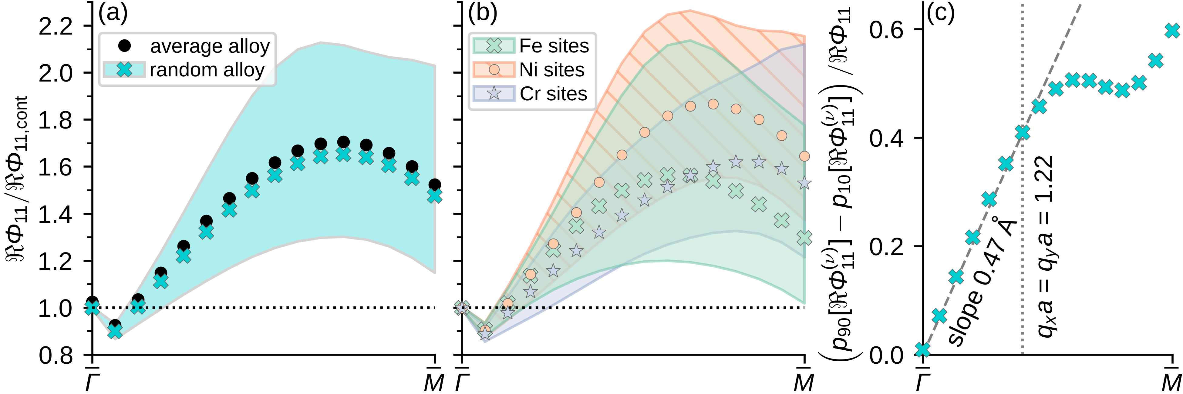
Figure 7: (a) Real part of $\Phi_{s,11}$ of average and true random FeNiCr, divided by the continuum solution; values along the diagonal $\bar{\Gamma}$-$\bar{M}$ of the first quadrant of the Brillouin zone; the shaded area shows the range between the 10th and 90th percentile of the site stiffness distribution in the random alloy; fluctuations in the random alloy go to zero as $\vec{q}\rightarrow\bar{\Gamma}$; the mean value and the average alloy stiffness approach the continuum stiffness; (b) (same y-axis as (a)) shows the mean value and the standard deviation of $\Phi^{(\nu)}_{11}$ in the random alloy for sites $\nu$ with different elements; the fluctuations go to zero as $\vec{q}\rightarrow\bar{\Gamma}$ and the mean values converge; (c) difference between the 90th and 10th percentile of $\Phi^{(\nu)}_{11}$, divided by the harmonic mean; the dashed line with a slope of $0.47\text{\,}\mathrm{\SIUnitSymbolAngstrom}\text{/}$ is the result of a linear least-squares fit between $\bar{\Gamma}$ and $q_{x}a{}=q_{y}a=1.22$ (wavelength $\lambda_{x}=\lambda_{y}\approx{}5a$).

IV Discussion

We observed that the average alloy accurately approximates the mean surface stiffness of the true random alloy over the surface Brillouin zone. The normal stiffness components $\Phi_{s,11}$, $\Phi_{s,22}$, and $\Phi_{s,33}$ are particularly important, because they generate the largest contributions to the force. The relative difference between the corresponding A-atom and and random alloy values is typically small. We observed the largest relative errors in $\Phi_{s,22}$ near $\bar{X}$, which represents the limit of short $x_{1}$-wavelength and infinite $x_{2}$-wavelength (and vice-versa by symmetry). However, the absolute value of $\Phi_{s,22}$ is also comparatively small between $\bar{\Gamma}$ and $\bar{X}$, yielding larger relative errors. $\Phi_{s,22}$ quickly increases with decreasing wavelength in $x_{2}$-direction and the relative error decreases. $\Phi_{s,11}$ behaves similarly near the upper corner of the Brillouin zone. Given that the overall errors are small over the full surface Brillouin zone, we conclude that the average alloy provides an accurate estimate of the mean forces on atoms in the random. This result is not surprising, since it was already shown in Ref. [27] that the A-atom has similar elastic constants as the corresponding true random alloy and the dependence of ${\mathbf{\Phi}}_{s}$ near the Brillouin-zone edge is determined primarily by lattice structure.

Another question is when continuum elasticity becomes a good approximation. This question can only be answered with respect to a relative measure that quantifies what we mean by “good”. Figure 7(a) shows such a relative measure for one of the components of the stiffness tensor. The point at $\bar{\Gamma}$ and next to it are affected by the finite depth of the sample, as they represent homogeneous deformation and deformation with a wavelength equal to the size of our box. The next two points have an error of around $10\%$ and correspond to an $x$- and $y$-wavelength of $15.5a$. It is fair to conclude that for distances beyond $\lambda_{c}\approx 15.5a$, the continuum approximation is reasonable. The decomposition into the individual atomic sites (Fig. 7(b)) underlines this behavior, as the individual stiffnesses for Fe, Ni and Cr sites converge to a unified value near the point where the continuum solution appears appropriate.

A connected question is how the per-site fluctuations decay as a function of wavevector. It is clear that at large wavelength, where the continuum approximation holds, the per-site variation of ${\mathbf{\Phi}}_{s}^{(\nu)}$ must be small. The per-site fluctuations are particularly small for the out-of-plane stiffness $\Phi_{s,33}$ (see Fig. 6(c)) where the continuum result has a lower error at intermediate wavelength as compared with the in-plane components $\Phi_{s,11}$ and $\Phi_{s,22}$ (Fig. 6(a)-(b)). The characteristic distance of $\lambda_{c}$ is therefore also a representative length beyond which per-site fluctuations become negligible. We now attempt a more quantitative analysis of this behavior. We divide the amplitude of the per-site fluctuations, as measured by the difference between the 90th and 10th percentile, by the stiffness matrix itself. As shown in Fig. 7(c), this ratio depends linearly on the wavevector $q$. Since $\Phi\propto q$, this implies that the amplitude of per-site fluctuations decays with wavelength $\lambda$ as $\lambda^{-2}$. This decay of the fluctuations should be compared to the decay of the error in quantitative stochastic homogenization [45, 46, 47], as shorter wavelengths are akin to taking smaller representative volumes of lateral length $\lambda$. Stochastic homogeneization predicts a scaling of $\lambda^{-2}$ for two-dimensional lattices.

Note that $\Phi_{s,33}$ is important for contact calculations [18, 20] while $\Phi_{s,11}$ and $\Phi_{s,22}$ are required for extended Peierls-Nabarro [48, 49] models of dislocations [50, 51] or sliding friction [52]. For dislocations in high-entropy alloys it is therefore of particular importance to capture the by-site fluctuations appropriately. Our results show that the A-atom potential could be used for calculating the mean response. The per-site fluctuations could then be obtained from the local structure within regions of size $\sim\lambda_{c}$ around the site of interest using perturbative approaches [53, 54, 55, 56, 57] or multipole expansions [58]. Since a local evaluation up to a cutoff distance scales linearly with the number of sites, this would give rise to a feasible computational scheme.

As a model materials, we have considered only the case of a random ternary alloy in this study. Our method is not limited to the ternary case, and we do not expect qualitative changes in other random alloys. We speculate that a decrease of fluctuations can be expected in alloys with short range order, where site occupations are correlated. The A-atom method assumes entirely uncorrelated site occupations, so it may fail to accurately predict the mean alloy surface stiffness in this case. There is also a simple practical limitation when it comes to calculating the surface stiffness of other alloys: a suitable potential needs to be available. This potential should have a continuous and smooth cutoff such that the Hessian is well-defined (i.e., does not exhibit jumps). It is known that cutoff schemes can lead to spurious effects, for example when calculating the phonon spectrum [59, 60], which also implicitly relies on the Hessian.

V Summary and Outlook

We have calculated the effective surface stiffness of unary crystals and a three-component random (high-entropy) alloys. Our results show that the surface stiffness has significant per-site variation near the edge of the surface Brillouin-zone, but that these variations disappear for larger wavelengths upon approach to the continuum limit. We identify a length of roughly $15.5$ atomic distances as the threshold where the continuum limit applies and per-site variations are small. At smaller distances, the average-atom approach of Varvenne and co-workers [27] accurately captures the mean response of the solid. Our results are a first step towards building multi-scale Peierls-Nabarro type models for dislocations in high-entropy alloys, that require an accurate model for the elastic response of the crystalline material that encloses the dislocation. The next step is to derive a perturbative expansion around the mean-field results presented here that allows the efficient calculation of per-site surface stiffnesses.

Appendix A Lattice parameters and elastic constants

The $0\text{\,}\mathrm{K}\text{/}$ FCC lattice parameter and cubic elastic constants of Ni, A-atom FeNiCr, and random FeNiCr are listed in table Tab. 1.

Table 1: $0\text{\,}\mathrm{K}\text{/}$ FCC lattice parameter and cubic elastic constants of pure Ni, FeNiCr equicomposition random alloy, and the corresponding average alloy, modeled using the EAM potential by Bonny et al. [39]

	pure Ni	random alloy	average alloy
$a_{0}$ ($\text{\,}\mathrm{\SIUnitSymbolAngstrom}\text{/}$)	$3.519\,294\,473\,157\,436\text{\,}\text{/}$	$3.521\,370\,324\,848\,13\text{\,}\text{/}$	$3.521\,818\,615\,513\,773\text{\,}\text{/}$
$C_{11}$ ($\text{\,}\mathrm{GPa}\text{/}$)	$246.929\,958\,899\,558\,983\text{\,}\text{/}$	$243.394\,832\,631\,828\,54\text{\,}\text{/}$	$246.610\,145\,262\,896\,367\text{\,}\text{/}$
$C_{12}$ ($\text{\,}\mathrm{GPa}\text{/}$)	$147.071\,946\,812\,490\,665\text{\,}\text{/}$	$157.446\,037\,329\,880\,62\text{\,}\text{/}$	$158.121\,884\,686\,608\,013\text{\,}\text{/}$
$C_{44}$ ($\text{\,}\mathrm{GPa}\text{/}$)	$125.030\,567\,589\,943\,999\text{\,}\text{/}$	$134.988\,584\,709\,745\,7\text{\,}\text{/}$	$138.525\,095\,411\,635\,675\text{\,}\text{/}$

The properties of Ni and A-atom FeNiCr were calculated in the same way. In order to determine the $0\text{\,}\mathrm{K}\text{/}$ FCC lattice parameter, we minimized the pressure of a fully periodic $5\times 5\times 5$ unit cell FCC crystal as a function of lattice parameter. The residual pressure was less than $1\text{\times}{10}^{-2}\text{\,}\mathrm{Pa}\text{/}$ in both cases. The elastic constants were computed by imposing ($1\text{\times}{10}^{-6}\text{\,}\text{/}$) strains $\varepsilon_{ij}$ on a $5\times 5\times 5$ unit cell FCC crystal and measuring the stress response $\sigma_{ij}$.

In the case of random FeNiCr, we prepared three $30\times 30\times 30$ unit cell configurations with random site occupations. As before, we determined the $0\text{\,}\mathrm{K}\text{/}$ lattice parameter by minimizing the pressure. However, the cell lengths along $x_{1}$, $x_{2}$, and $x_{3}$ were adjusted independently, and so each calculation yields three values for the lattice parameter. The value listed in Tab. 1 is the average over spatial directions and samples. In order to determine the elastic constants, we imposed simple shear strain $\varepsilon_{12}$ and uni-axial normal strain $\varepsilon_{22}$ on the samples and measured the stress response. In the case of uniaxial tension/compression, Hooke’s law yields

$$\sigma_{22} =C_{22}\varepsilon_{22},$$ (19)

$$\sigma_{11} =C_{12}\varepsilon_{22},$$ (20)

$$\sigma_{33} =C_{23}\varepsilon_{22},$$ (21)

where $C_{12}=C_{23}$ for cubic materials. In the case of simple shear

$$\sigma_{12}=C_{44}\varepsilon_{12}.$$ (22)

We applied positive and negative shear, as well as tension and compression, with absolute values in the range $1\text{\times}{10}^{-9}1\text{\times}{10}^{-4}$.

Appendix B Hessian matrix within the embedded atom method

Below, we present the analytical solution for the Hessian matrix of the total potential energy in the EAM approximation. Greek superscripts refer to atom identifiers. For $N$ consecutively numbered atoms $\mu,\nu,\gamma,\delta\in[1,N]$. Lowercase roman subscripts refer to the components of a vector or tensor with respect to the three axes of a Cartesian coordinate system, i.e. $i,j\in[1,2,3]$. $x_{i}^{(\nu)}$ is the coordinate of atom $\nu$ in direction $i$. The $i$-component of the distance vector between atoms $\nu$ and $\mu$ is

$$x_{i}^{(\nu\mu{})}=x_{i}^{(\mu{})}-x_{i}^{(\nu{})}.$$ (23)

The absolute value of the distance vector is

$$x^{(\nu\mu{})} =\left(\left(x_{1}^{(\nu\mu{})}\right)^{2}+\left(x_{2}^{(\nu\mu{})}\right)^{2}+\left(x_{3}^{(\nu\mu{})}\right)^{2}\right)^{1/2}.$$ (24)

Furthermore, we use the abbreviations

$$\tilde{x}_{i}^{(\nu\mu{})} \equiv\frac{x_{i}^{(\nu\mu{})}}{x^{(\nu\mu)}}\quad\text{and}$$ (25)

$$\tilde{s}_{ij}^{(\nu{}\mu{})} \equiv\tilde{x}_{i}^{(\nu\mu{})}\tilde{x}_{j}^{(\nu\mu{})}.$$ (26)

The two symbols represent a normalized distance vector and the outer product of a normalized distance vector with itself, respectively. The expression for the Hessian involves the following derivatives of a pair distance vector and its absolute value:

$$\frac{\partial x_{i}^{(\gamma\delta{})}}{\partial x_{j}^{(\mu{})}} =\delta_{ij}\left(\delta_{\mu\delta}-\delta_{\mu\gamma}\right),$$ (27)

$$\frac{\partial x^{(\gamma\delta)}}{\partial x_{i}^{(\nu)}} =\tilde{x}_{i}^{(\gamma{}\delta{})}\left(\delta_{\delta\nu}-\delta_{\gamma\nu}\right),$$ (28)

where $\delta_{ij}$ is Kronecker’s delta, i.e. $\delta_{ij}=1$ if $i=j$ and $\delta_{ij}=0$ otherwise.

In the EAM, the total potential energy $\mathcal{V}^{\mathrm{int}}$ due to interaction between atoms is the sum of pair and embedding energy contributions [26],

$$\mathcal{V}^{\mathrm{int}} =\mathcal{V}^{\mathrm{pair}}+\mathcal{V}^{\mathrm{embed}}.$$ (29)

The pair energy contribution is

$$\mathcal{V}^{\mathrm{pair}} =\frac{1}{2}\sum_{\gamma}^{N}\sum_{\delta\neq\gamma}^{N}{\phi^{(\gamma\delta)}}\left(x^{(\gamma\delta)}\right),$$ (30)

where ${\phi^{(\nu\mu)}}\left(x^{(\gamma\delta)}\right)$ is the pair potential of atoms $\mu$ and $\nu$, evaluated at $x^{(\gamma\delta)}$. For the sake of brevity, we use the abbreviation $\phi^{(\gamma\delta)}\equiv{\phi^{(\gamma\delta)}}\left(x^{(\gamma\delta)}\right)$ in the following.

The embedding energy contribution is

$$\mathcal{V}^{\mathrm{embed}}=\sum_{\gamma}^{N}{U^{(\gamma)}}\left({\rho^{(\gamma)}}\right),$$ (31)

where ${U^{(\gamma)}}$ is the embedding energy functional of atom $\gamma$. ${U^{(\gamma)}}$ is a functional of the total electron density at the site of $\gamma$, which is computed as

$${\rho^{(\gamma)}} =\sum_{\delta\neq\gamma}^{N}{g^{(\delta)}}\left(x^{(\gamma\delta)}\right),$$ (32)

where ${g^{(\delta)}}\left(x^{(\gamma\delta)}\right)$ is the electron density function of atom $\delta$. For the sake of brevity, we write ${g^{(\gamma\delta)}}\equiv{g^{(\delta)}}\left(x^{(\gamma\delta)}\right)$.

The Hessian matrix $\mathbf{H}$ is the $3N\times{}3N$ matrix of second derivatives of $\mathcal{V}^{\mathrm{int}}$ with respect to the coordinates of the atoms. The components of $\mathbf{H}$ are

$$H_{(3(\nu{}-1)+i)(3(\mu{}-1)+j)}=\frac{\partial^{2}\mathcal{V}^{\mathrm{int}}}{\partial x_{i}^{(\nu{})}\partial x_{j}^{(\mu{})}}.$$ (33)

We first write the gradient of $\mathcal{V}^{\mathrm{int}}$. In the following, we use one and two dashes, respectively, to indicate the first and second derivatives of a function, e.g. ${{g^{(\delta)}}}^{\prime}\left(x^{(\gamma\delta)}\right)\equiv d{{g^{(\delta)}}}(x^{(\gamma\delta)})/dx^{(\gamma\delta)}$ and ${{g^{(\delta)}}}^{\prime\prime}\left(x^{(\gamma\delta)}\right)\equiv d^{2}{g^{(\delta)}}(x^{(\gamma\delta)})/d(x^{(\gamma\delta)})^{2}$. As before, we abbreviate the dependence on $x^{(\gamma\delta)}$ by writing ${{g^{(\gamma\delta)}}}^{\prime}\equiv{{g^{(\delta)}}}^{\prime}\left(x^{(\gamma\delta)}\right)$ and ${{\phi^{(\gamma\delta)}}}^{\prime}\equiv{{\phi^{(\gamma\delta)}}}^{\prime}\left(x^{(\gamma\delta)}\right)$, and likewise for the second derivative. With this notation, the expression for the gradient of $\mathcal{V}^{\mathrm{int}}$ becomes

$$\begin{aligned} \frac{\partial\mathcal{V}^{\mathrm{int}}}{\partial x_{i}^{(\nu)}}&=\frac{\partial\mathcal{V}^{\mathrm{pair}}}{\partial x_{i}^{(\nu)}}+\frac{\partial\mathcal{V}^{\mathrm{embed}}}{\partial x_{i}^{(\nu)}}\\ &=-\sum_{\gamma\neq\nu}^{N}\left({\phi^{(\gamma\nu)}}^{\prime}+{U^{(\gamma)}}^{\prime}{g^{(\gamma\nu)}}^{\prime}+{U^{(\nu)}}^{\prime}{g^{(\nu\gamma)}}^{\prime}\right)\tilde{x}_{i}^{(\nu\gamma)}.\end{aligned}$$ (34)

Like the gradient, the Hessian matrix can be split into contributions from $\mathcal{V}^{\mathrm{pair}}$ and $\mathcal{V}^{\mathrm{embed}}$,

$$\frac{\partial^{2}\mathcal{V}^{\mathrm{int}}}{\partial x_{i}^{(\nu)}\partial x_{j}^{(\mu)}}=\frac{\partial^{2}\mathcal{V}^{\mathrm{pair}}}{\partial x_{i}^{(\nu)}\partial x_{j}^{(\mu)}}+\frac{\partial^{2}\mathcal{V}^{\mathrm{embed}}}{\partial x_{i}^{(\nu)}\partial x_{j}^{(\mu)}}.$$ (35)

The pair contribution is

$$\begin{aligned} \frac{\partial^{2}\mathcal{V}^{\mathrm{pair}}}{\partial x_{i}^{(\nu)}\partial x_{j}^{(\mu)}}=&-{\phi^{(\nu\mu)}}^{\prime\prime}\tilde{s}_{ij}^{(\nu{}\mu{})}-\frac{{\phi^{(\nu\mu)}}^{\prime}}{x^{(\nu\mu)}}\left(\delta_{ij}-\tilde{s}_{ij}^{(\nu{}\mu{})}\right)\\ &+\delta_{\nu\mu}\sum_{\gamma\neq\nu}^{N}{\phi^{(\nu\gamma)}}^{\prime\prime}\tilde{s}_{ij}^{(\nu{}\gamma{})}\\ &+\delta_{\nu\mu}\sum_{\gamma\neq\nu}^{N}\frac{{\phi^{(\nu\gamma)}}^{\prime}}{x^{(\nu\gamma)}}\left(\delta_{ij}-\tilde{s}_{ij}^{(\nu{}\gamma{})}\right).\end{aligned}$$ (36)

The third and the fourth term are the sums of the first and second term, respectively, over the neighbors of $\nu$. This expression is equal to the Hessian matrix for a pair potential, see Ref. [20].

The embedding contribution is the sum of eight terms,

$$\frac{\partial^{2}\mathcal{V}^{\mathrm{embed}}}{\partial x_{i}^{(\nu)}\partial x_{j}^{(\mu)}} =\sum_{n=1}^{8}\prescript{n}{}{T}_{ij}^{(\nu{}\mu{})},$$ (37)

where

$$\prescript{1}{}{T}_{ij}^{(\nu{}\mu{})} =\delta_{\nu\mu}{U^{(\nu)}}^{\prime\prime}\sum_{\gamma\neq\nu}^{N}{g^{(\nu\gamma)}}^{\prime}x_{i}^{(\nu\gamma{})}\sum_{\gamma\neq\nu}^{N}{g^{(\nu\gamma)}}^{\prime}x_{j}^{(\nu\gamma{})},$$ (38)

$$\prescript{2}{}{T}_{ij}^{(\nu{}\mu{})} =-{U^{(\nu)}}^{\prime\prime}{g^{(\nu\mu)}}^{\prime}x_{j}^{(\nu\mu)}\sum_{\gamma\neq\nu}^{N}{g^{(\nu\gamma)}}^{\prime}x_{i}^{(\nu\gamma)},$$ (39)

$$\prescript{3}{}{T}_{ij}^{(\nu{}\mu{})} ={U^{(\mu)}}^{\prime\prime}{g^{(\mu\nu)}}^{\prime}x_{i}^{(\nu\mu{})}\sum_{\gamma\neq\mu}^{N}{g^{(\mu\gamma)}}^{\prime}x_{j}^{(\mu\gamma{})},$$ (40)

$$\prescript{4}{}{T}_{ij}^{(\nu{}\mu{})} =-\left({U^{(\mu)}}^{\prime}{g^{(\mu\nu)}}^{\prime\prime}+{U^{(\nu)}}^{\prime}{g^{(\nu\mu)}}^{\prime\prime}\right)\tilde{s}_{ij}^{(\nu{}\mu{})},$$ (41)

$$\prescript{5}{}{T}_{ij}^{(\nu{}\mu{})} =\delta_{\nu\mu}\sum_{\gamma\neq\nu}^{N}\left({U^{(\gamma)}}^{\prime}{g^{(\gamma\nu)}}^{\prime\prime}+{U^{(\nu)}}^{\prime}{g^{(\nu\gamma)}}^{\prime\prime}\right)\tilde{s}_{i{}j}^{(\nu{}\gamma{})},$$ (42)

$$\prescript{6}{}{T}_{ij}^{(\nu{}\mu{})} =-\frac{{U^{(\mu)}}^{\prime}{g^{(\mu\nu)}}^{\prime}+{U^{(\nu)}}^{\prime}{g^{(\nu\mu)}}^{\prime}}{x^{(\nu\mu)}}\left(\delta_{ij}-\tilde{s}_{i{}j}^{(\nu{}\mu{})}\right),\$$ (43)

$$\prescript{7}{}{T}_{ij}^{(\nu{}\mu{})} =\delta_{\nu\mu}\sum_{\gamma\neq\nu}^{N}\frac{{U^{(\gamma)}}^{\prime}{g^{(\gamma\nu)}}^{\prime}+{U^{(\nu)}}^{\prime}{g^{(\nu\gamma)}}^{\prime}}{x^{(\nu\gamma)}}\left(\delta_{ij}-\tilde{s}_{ij}^{(\nu{}\gamma{})}\right),$$ (44)

and

$$\prescript{8}{}{T}_{ij}^{(\nu{}\mu{})} =\sum_{\begin{subarray}{c}\gamma\neq\nu\\ \gamma\neq\mu\end{subarray}}^{N}{U^{(\gamma)}}^{\prime\prime}{g^{(\gamma\nu)}}^{\prime}{g^{(\gamma\mu)}}^{\prime}\frac{x_{i}^{(\gamma\nu)}}{x^{(\gamma\nu)}}\frac{x_{j}^{(\gamma\mu)}}{x^{(\gamma\mu)}}.$$ (45)

Note that the terms remain the same when the index pairs $(i,\nu)$ and $(j,\mu)$ are interchanged, which is necessary for the Hessian to be symmetric. Terms $\prescript{5}{}{T}_{ij}^{(\nu{}\mu{})}$ and $\prescript{7}{}{T}_{ij}^{(\nu{}\mu{})}$ are the sums of terms $\prescript{4}{}{T}_{ij}^{(\nu{}\mu{})}$ and $\prescript{6}{}{T}_{ij}^{(\nu{}\mu{})}$, respectively, over the neighbors of atom $\nu$. Terms $\prescript{1}{}{T}_{ij}^{(\nu{}\mu{})}$–$\prescript{7}{}{T}_{ij}^{(\nu{}\mu{})}$ are zero if atoms $\mu$ and $\nu$ are not neighbors, i.e. if $r_{\mu\nu}>r_{\mathrm{cut}}$, where $r_{\mathrm{cut}}$ is the cutoff radius of the potential. Term $\prescript{8}{}{T}_{ij}^{(\nu{}\mu{})}$ is the most complex term. In order to compute this term, one needs to determine the common neighbors of atoms $\mu$ and $\nu$, even if $\mu$ and $\nu$ are not neighbors themselves.

Appendix C Surface Green’s function for an anisotropic elastic continuum of finite thickness

No closed form solution for the surface Green’s function of the anistropic elastic continuum exists. We here compute this Green’s function semi-analytically. Starting from the definition of the (small-strain) strain tensor,

$$\varepsilon_{ij}=\frac{1}{2}\left(\partial_{i}u_{j}+\partial_{j}u_{i}\right)$$ (46)

where $\vec{u}(x_{1},x_{2},x_{3}{})$ is the displacement field, we obtain the stress tensor as

$$\sigma_{ij}=C_{ijkl}\varepsilon_{kl}=\frac{1}{2}C_{ijkl}\left(\partial_{k}u_{l}+\partial_{l}u_{k}\right)=C_{ijkl}\partial_{k}u_{l}.$$ (47)

$C_{ijkl}$ is the fourth-order tensor of elastic constants with at most $27$ independent component. Note that $\partial_{i}$ indicates the partial derivative in direction $i$ and Einstein summation convention applies to all Latin indices in this paper. The usual symmetry relationships

$$C_{ijkl}=C_{jikl}\text{,}\quad C_{ijkl}=C_{ijlk}\quad\text{and}\quad C_{ijkl}=C_{klij}$$ (48)

have been used to obtain the last equality in Eq. (47). Elastostatic equilibrium dictates $\partial_{i}\sigma_{ij}=0$. Inserting Eqs. (47) into this expression yield the generalization of the Navier-Lamé equations,

$$\partial_{j}\left(C_{ijkl}\partial_{k}u_{l}\right)=C_{ijkl}\partial_{j}\partial_{k}u_{l}=0,$$ (49)

where we have assumed that $C_{ijkl}$ does not depend on position, i.e. we are dealing with a homogeneous half-space.

We now search for a solution of the displacements $\vec{u}_{s}(x_{1},x_{2})$ within the plane of a surface subject to the traction boundary conditions $P(x_{1},x_{2})$, $Q_{1}(x_{1},x_{2})$ and $Q_{2}(x_{1},x_{2})$. With $\vec{Q}=(Q_{1},Q_{2},P)$, the displacements are given by $\vec{u}_{s}(x_{1},x_{2})=\int dx_{1}^{\prime}dx_{2}^{\prime}\,{\mathbf{G}}_{s}(x_{1}-x_{1}^{\prime},x_{2}-x_{2}^{\prime})\cdot\vec{Q}(x_{1}^{\prime},x_{2}^{\prime})$. It is usually convenient to state the Fourier transform of this expression, $\vec{u}_{s}(\vec{q})={\mathbf{G}}_{s}(\vec{q})\cdot\vec{Q}(\vec{q})$ where $\vec{q}=({q_{1}},{q_{2}})$ is the wavevector within the plane of the surface. ${\mathbf{G}}_{s}$ is the surface Green’s function.

Note that Eq. (49) is a set of three linear partial differential equations for the three components of the displacement field $\vec{u}(x_{1},x_{2},x_{3}{})$ throughout the body. We are only interested in $\vec{u}_{s}(x_{1},x_{2})=\vec{u}(x_{1},x_{2},0)$. We can write Eq. (49) as [64]

$$M_{il}u_{l}=0$$ (50)

with the linear operator

$$M_{il}=C_{ijkl}\partial_{j}\partial_{k}.$$ (51)

Because of Eq. (48), the operator $\mathbf{M}$ is symmetric, $M_{il}=M_{li}$. In order to obtain the surface Green’s function, we need to impose the traction boundary conditions $P$, $Q_{1}$ and $Q_{2}$. At the surface ($x_{3}=0$), the stress tensor fulfills

$$\begin{aligned} \sigma_{33}(x_{1},x_{2},x_{3}=0)&=P(x_{1},x_{2})\text{,}\\ \sigma_{13}(x_{1},x_{2},x_{3}=0)&=Q_{1}(x_{1},x_{2})\quad\text{and}\\ \sigma_{23}(x_{1},x_{2},x_{3}=0)&=Q_{2}(x_{1},x_{2}).\end{aligned}$$ (52)

To solve Eq. (50) numerically under the boundary conditions given by Eq. (52), we need to transform Eq. (51) into an algebraic equation. Because we are interested in the solution for a plane interface, we have translational invariance in the $x_{1}$-$x_{2}$ plane. The Fourier transform of Eq. (51) in this plane is given by

$$\begin{aligned} M_{il}=&-C_{i11l}{{q_{1}}}^{2}-C_{i22l}{{q_{2}}}^{2}-(C_{i12l}+C_{i21l}){q_{1}}{q_{2}}\\ &+\left[i(C_{i13l}+C_{i31l}){q_{1}}+i(C_{i23l}+C_{i32l}){q_{2}}\right]\partial_{{3}}\\ &+C_{i33l}{\partial_{{3}}}^{2},\end{aligned}$$ (53)

where ${q_{1}}$ and ${q_{2}}$ are the wavevectors in this plane. Any nontrivial solution to the homogeneous equation Eq. (50) must fulfill $\det\mathbf{M}=0$. This fixes the admissible values of the eigenvalue $i{q_{3}}$ of the operator $\partial_{{3}}$. Since $\det\mathbf{M}$ is a sixth-order even polynomial in $i{q_{3}}$, for each ${q_{1}},{q_{2}}$, we obtain six values for $i{{q_{3}}}^{(\alpha)}$ that occur in symmetric pairs.

For six eigenvalues ${{q_{3}}}^{(\alpha)}$ the displacement field is given by a superposition of the basis functions $\vec{\eta}^{(\alpha)}e^{i{{q_{3}}}^{(\alpha)}x_{3}}$, where $\vec{\eta}^{(\alpha)}$ is the solution of $\mathbf{M}\cdot\vec{\eta}^{(\alpha)}e^{i{{q_{3}}}^{(\alpha)}x_{3}}=0$. It is straightforward solve for both ${{q_{3}}}^{(\alpha)}$ and $\vec{\eta}^{(\alpha)}$ numerically. The general displacement field is then given by

$$\vec{u}=\sum_{\alpha}c_{\alpha}\vec{\eta}^{(\alpha)}e^{i{q_{3}}^{(\alpha)}x_{3}}=\mathbf{U}({q_{1}},{q_{2}},x_{3})\cdot\vec{c}$$ (54)

with generally $\vec{c}=(c_{1},c_{2},c_{3},c_{4},c_{5},c_{6})$ and $U_{k\alpha}({q_{1}},{q_{2}},x_{3})=\eta_{k}^{(\alpha)}e^{i{{q_{3}}}^{(\alpha)}x_{3}}$ where $\eta_{k}^{(\alpha)}$ and ${{q_{3}}}^{(\alpha)}$ depend implicitly on ${q_{1}}$ and ${q_{2}}$. The constants $c_{\alpha}$ are now obtained from the displacement or traction boundary conditions on both top and bottom of the half-space.

For an infinite half-space, all $c_{\alpha}$ for $\Im{q_{3}}^{(\alpha)}<0$ must vanish because the solution diverges as ${q_{3}}\to\infty$. This leaves us with three relevant basis functions, that we label (without loss of generality) by $\alpha=1,2,3$ (and hence $c_{4}=c_{5}=c_{6}=0$). The traction boundary condition, Eq. (52), becomes

$$Q_{1}({q_{1}},{q_{2}}) =iC_{13kl}q_{k}u_{l}=i\sum_{\alpha}C_{13kl}q_{k}^{(\alpha)}\eta_{l}^{(\alpha)}c_{\alpha}$$ (55)

$$Q_{2}({q_{1}},{q_{2}}) =iC_{23kl}q_{k}u_{l}=i\sum_{\alpha}C_{23kl}q_{k}^{(\alpha)}\eta_{l}^{(\alpha)}c_{\alpha},$$ (56)

$$P({q_{1}},{q_{2}}) =iC_{33kl}q_{k}u_{l}=i\sum_{\alpha}C_{33kl}q_{k}^{(\alpha)}\eta_{l}^{(\alpha)}c_{\alpha}$$ (57)

or in matrix notation

$$\vec{Q}({q_{1}},{q_{2}})=\mathbf{F}({q_{1}},{q_{2}})\cdot\vec{c}$$ (58)

with $F_{j\alpha}({q_{1}},{q_{2}})=iC_{j\textbf{}3kl}q_{k}^{(\alpha)}\eta_{l}^{(\alpha)}$ and ${{q_{1}}}^{(\alpha)}\equiv{q_{1}}$ and ${{q_{2}}}^{(\alpha)}\equiv{q_{2}}$. Combining Eqs. (54) and (58) gives ${\mathbf{G}}_{s}({q_{1}},{q_{2}})=\mathbf{U}({q_{1}},{q_{2}},0)\cdot\mathbf{F}^{-1}({q_{1}},{q_{2}})$ or ${\mathbf{\Phi}}_{s}={\mathbf{G}}_{s}^{-1}=\mathbf{F}\cdot\mathbf{U}^{-1}$.

For a finite half-space, we need to keep all six basis functions $\alpha\in[1\ldots 6]$ and require in addition a boundary condition at the bottom of the substrate. We here only discuss fixed displacement, in particular $u_{i}(x_{1},x_{2},x_{3}=h)=0$ where $h$ is the thickness of the elastic substrate. In addition to Eqs. (55) to (57), the displacement boundary condition leads to the additional equations

$$\sum_{\alpha}c_{\alpha}\eta_{j}^{(\alpha)}e^{i{{q_{3}}}^{(\alpha)}h}=u_{b,j}$$ (59)

for $j=1,2,3$. Here $\vec{u}_{b}$ are the displacements at the bottom of the substrate. In dyadic notation this becomes

$$\vec{\varphi}({q_{1}},{q_{2}})=\mathbf{F}_{h}({q_{1}},{q_{2}})\cdot\vec{c}$$ (60)

where $\vec{\varphi}$ contains forces at the top and displacements at the bottom of the substrate. $\mathbf{F}_{h}$ is a $6\times 6$ matrix. The Green’s function is then given by the first three columns of $\mathbf{U}\cdot\mathbf{F}_{h}^{-1}$.

Note that for the (special) isotropic case where $C_{ijkl}=\lambda\delta_{ij}\delta_{kl}+2\mu\delta_{ik}\delta_{jl}$ with Lamé constants $\lambda$ and $\mu$, the solution of $\det\mathbf{M}=0$ is degenerate, $i{q_{3}}=\pm\sqrt{{q_{1}}^{2}+{q_{2}}^{2}}$, and the above analysis does not apply. The displacement field is then given by superposition of the basis functions $e^{i{q_{3}}x_{3}}$, $x_{3}e^{i{q_{3}}x_{3}}$, ${x_{3}}^{2}e^{i{q_{3}}x_{3}}$, $e^{-i{q_{3}}x_{3}}$, $x_{3}e^{-i{q_{3}}x_{3}}$ and ${x_{3}}^{2}e^{-i{q_{3}}x_{3}}$. The close-form solution for the infinite half-space in this limit is described in Ref. [10]. It yields the surface Green’s function

$$\mu{\mathbf{G}}_{s}(\vec{q})=\begin{pmatrix}\frac{1}{q}-\frac{\nu{{q_{1}}}^{2}}{q^{3}}&-\frac{\nu{q_{1}}{q_{2}}}{q^{3}}&i\frac{(1-2\nu){q_{1}}}{2q^{2}}\\ -\frac{\nu{q_{1}}{q_{2}}}{q^{3}}&\frac{1}{q}-\frac{\nu{{q_{2}}}^{2}}{q^{3}}&i\frac{(1-2\nu){q_{2}}}{2q^{2}}\\ -i\frac{(1-2\nu){q_{1}}}{2q^{2}}&-i\frac{(1-2\nu){q_{2}}}{2q^{2}}&\frac{1-\nu}{q}\\ \end{pmatrix}$$ (61)

with Poisson number $\nu=\lambda/[2(\lambda+\mu)]$. Inverse Fourier transform of Eq. (61) leads to the well-known potential functions of Boussinesq & Cerruti [3].

References

- Tadmor and Miller [2011] E. B. Tadmor and R. E. Miller, Modeling materials: Continuum, atomistic and multiscale techniques (Cambridge University Press, 2011).
- Bulatov et al. [2006] V. V. Bulatov, V. Bulatov, and W. Cai, Computer Simulations of Dislocations (Oxford University Press, 2006).
- Johnson [1985] K. L. Johnson, Contact Mechanics (Cambridge University Press, 1985).
- Kohlhoff et al. [1991] S. Kohlhoff, P. Gumbsch, and H. F. Fischmeister, Crack propagation in b.c.c. crystals studied with a combined finite-element and atomistic model, Philosophical Magazine A 64, 851 (1991).
- Tadmor et al. [1996] E. B. Tadmor, M. Ortiz, and R. Phillips, Quasicontinuum analysis of defects in solids, Philosophical Magazine A 73, 1529 (1996).
- Shenoy et al. [1998] V. B. Shenoy, R. Miller, E. B. Tadmor, R. Phillips, and M. Ortiz, Quasicontinuum models of interfacial structure and deformation, Physical Review Letters 80, 742 (1998).
- Xiao and Belytschko [2004] S. Xiao and T. Belytschko, A bridging domain method for coupling continua with molecular dynamics, Computer Methods Applied Mechanics and Engineering 193, 1645 (2004).
- Badia et al. [2007] S. Badia, P. Bochev, R. Lehoucq, M. Parks, J. Fish, M. A. Nuggehally, and M. Gunzburger, A force-based blending model foratomistic-to-continuum coupling, International Journal for Multiscale Computational Engineering 5, 387 (2007).
- Chen et al. [2019] Y. Chen, S. Shabanov, and D. L. McDowell, Concurrent atomistic-continuum modeling of crystalline materials, Journal of Applied Physics 126, 101101 (2019).
- Amba-Rao [1969] C. L. Amba-Rao, Fourier transform methods in elasticity problems and an application, Journal of the Franklin Institute 287, 241 (1969).
- Kalker and Randen [1972] J. J. Kalker and Y. Randen, A minimum principle for frictionless elastic contact with application to non-Hertzian half-space contact problems, Journal of Engineering Mathematics 6, 193 (1972).
- Stanley and Kato [1997] H. M. Stanley and T. Kato, An FFT-based method for rough surface contact, Journal Tribology 119, 481 (1997).
- Hodapp et al. [2019] M. Hodapp, G. Anciaux, and W. Curtin, Lattice green function methods for atomistic/continuum coupling: Theory and data-sparse implementation, Computer Methods in Applied Mechanics and Engineering 348, 1039 (2019).
- Sinclair [1971] J. E. Sinclair, Improved atomistic model of a bcc dislocation core, Journal of Applied Physics 42, 5321 (1971).
- Sinclair et al. [1978] J. E. Sinclair, P. C. Gehlen, R. G. Hoagland, and J. P. Hirth, Flexible boundary conditions and nonlinear geometric effects in atomic dislocation modeling, Journal of Applied Physics 49, 3890 (1978).
- Gallego and Ortiz [1993] R. Gallego and M. Ortiz, A harmonic/anharmonic energy partition method for lattice statics computations, Modelling and Simulation in Materials Science and Engineering 1, 417 (1993).
- Li [2009] X. Li, Efficient boundary conditions for molecular statics models of solids, Physical Review B 80, 104112 (2009).
- Campañá and Müser [2006] C. Campañá and M. H. Müser, Practical Green’s function approach to the simulation of elastic semi-infinite solids, Physical Review B 74, 075420 (2006).
- Trinkle [2008] D. R. Trinkle, Lattice green function for extended defect calculations: Computation and error estimation with long-range forces, Physical Review B 78, 014110 (2008).
- Pastewka et al. [2012] L. Pastewka, T. A. Sharp, and M. O. Robbins, Seamless elastic boundaries for atomistic calculations, Physical Review B 86, 075459 (2012).
- Miller and Tadmor [2009] R. E. Miller and E. B. Tadmor, A unified framework and performance benchmark of fourteen multiscale atomistic/continuum coupling methods, Modelling and Simulation in Materials Science and Engineering 17, 053001 (2009).
- Kajita et al. [2012] S. Kajita, H. Washizu, and T. Ohmori, Simulation of solid-friction dependence on number of surface atoms and theoretical approach for infinite number of atoms, Physical Review B 86, 1 (2012).
- Kajita [2016] S. Kajita, Green’s function nonequilibrium molecular dynamics method for solid surfaces and interfaces, Physical Review E 94, 033301 (2016).
- Monti et al. [2021] J. M. Monti, L. Pastewka, and M. O. Robbins, Green’s function method for dynamic contact calculations, Physical Review E (2021), in review.
- Kong et al. [2009] L. T. Kong, G. Bartels, C. Campañá, C. Denniston, and M. H. Müser, Implementation of Green’s function molecular dynamics: An extension to LAMMPS, Computer Physics Communications 180, 1004 (2009).
- Daw and Baskes [1984] M. S. Daw and M. Baskes, Embedded-atom method: Derivation and application to impurities, surfaces, and other defects in metals, Physical Review B 29, 6443 (1984).
- Varvenne et al. [2016] C. Varvenne, A. Luque, W. G. Nöhring, and W. A. Curtin, Average-atom interatomic potential for random alloys, Physical Review B 93, 104201 (2016).
- [28] matscipy: Materials science with Python at the atomic-scale, https://github.com/libAtoms/matscipy.
- Balay et al. [2019] S. Balay, S. Abhyankar, M. F. Adams, J. Brown, P. Brune, K. Buschelman, L. Dalcin, V. Eijkhout, W. D. Gropp, D. Karpeyev, D. Kaushik, M. G. Knepley, D. A. May, L. C. McInnes, R. T. Mills, T. Munson, K. Rupp, P. Sanan, B. F. Smith, S. Zampini, H. Zhang, and H. Zhang, PETSc Users Manual, Tech. Rep. ANL-95/11 - Revision 3.11 (Argonne National Laboratory, 2019).
- Balay et al. [1997] S. Balay, W. D. Gropp, L. C. McInnes, and B. F. Smith, Efficient management of parallelism in object oriented numerical software libraries, in Modern Software Tools in Scientific Computing, edited by E. Arge, A. M. Bruaset, and H. P. Langtangen (Birkhäuser Press, 1997) pp. 163–202.
- Amestoy et al. [2001] P. Amestoy, I. S. Duff, J. Koster, and J.-Y. L’Excellent, A fully asynchronous multifrontal solver using distributed dynamic scheduling, SIAM Journal on Matrix Analysis and Applications 23, 15 (2001).
- Amestoy et al. [2019] P. Amestoy, A. Buttari, J.-Y. L’Excellent, and T. Mary, Performance and scalability of the block low-rank multifrontal factorization on multicore architectures, ACM Transactions on Mathematical Software 45, 2:1 (2019).
- Amestoy et al. [2015] P. R. Amestoy, I. S. Duff, J.-Y. L’Excellent, and F.-H. Rouet, Parallel computation of entries of , SIAM Journal on Scientific Computing 37, C268 (2015).
- Song et al. [2017] H. Song, F. Tian, Q.-M. Hu, L. Vitos, Y. Wang, J. Shen, and N. Chen, Local lattice distortion in high-entropy alloys, Physical Review Materials 1, 023404 (2017).
- Owen and Jones [2018] L. R. Owen and N. G. Jones, Lattice distortions in high-entropy alloys, Journal of Materials Research 33, 2954 (2018).
- Owen and Jones [2020] L. Owen and N. Jones, Quantifying local lattice distortions in alloys, Scripta Materialia 187, 428 (2020).
- Kozlov [1979] S. M. Kozlov, The averaging of random operators, Mat. Sb. (N.S.) 109(151), 188 (1979).
- Papanicolaou and Varadhan [1981] G. C. Papanicolaou and S. R. S. Varadhan, Boundary value problems with rapidly oscillating random coefficients, in Random fields, Vol. I, II (Esztergom, 1979), Colloq. Math. Soc. János Bolyai, Vol. 27 (North-Holland, Amsterdam-New York, 1981) pp. 835–873.
- Bonny et al. [2011] G. Bonny, D. Terentyev, R. C. Pasianot, S. Poncé, and A. Bakaev, Interatomic potential to study plasticity in stainless steels: the FeNiCr model alloy, Modelling and Simulation in Materials Science and Engineering 19, 085008 (2011).
- Smith and Was [1989] R. W. Smith and G. S. Was, Application of molecular dynamics to the study of hydrogen embrittlement in Ni-Cr-Fe alloys, Physical Review B 40, 10332 (1989).
- Bitzek et al. [2006] E. Bitzek, P. Koskinen, F. Gähler, M. Moseler, and P. Gumbsch, Structural relaxation made simple, Physical Review Letters 97, 170201 (2006).
- Guénolé et al. [2020] J. Guénolé, W. G. Nöhring, A. Vaid, F. Houllé, Z. Xie, A. Prakash, and E. Bitzek, Assessment and optimization of the fast inertial relaxation engine (fire) for energy minimization in atomistic simulations and its implementation in lammps, Computational Materials Science 175, 109584 (2020).
- Barber [1992] J. Barber, Elasticity (Springer Netherlands, Dordrecht, 1992).
- [44] ContactMechanics: Contact mechanics using elastic half-space methods, https://github.com/ComputationalMechanics/ContactMechanics.
- Gloria and Otto [2011] A. Gloria and F. Otto, An optimal variance estimate in stochastic homogenization of discrete elliptic equations, The Annals of Probability 39, 779 (2011), 1104.1291 .
- Gloria et al. [2013] A. Gloria, S. Neukamm, and F. Otto, Quantification of ergodicity in stochastic homogenization: optimal bounds via spectral gap on Glauber dynamics, Inventiones mathematicae 199, 455 (2013).
- Armstrong et al. [2019] S. Armstrong, T. Kuusi, and J.-C. Mourrat, Quantitative stochastic homogenization and large-scale regularity, Grundlehren der Mathematischen Wissenschaften [Fundamental Principles of Mathematical Sciences], Vol. 352 (Springer, Cham, 2019) pp. xxxviii+518.
- Peierls [1940] R. Peierls, The size of a dislocation, Proceedings of the Physical Society 52, 34 (1940).
- Nabarro [1947] F. R. N. Nabarro, Dislocations in a simple cubic lattice, Proceedings of the Physical Society 59, 256 (1947).
- Sharp et al. [2016] T. A. Sharp, L. Pastewka, and M. O. Robbins, Elasticity limits structural superlubricity in large contacts, Physical Review B 93, 121402(R) (2016).
- Sharp et al. [2017] T. A. Sharp, L. Pastewka, V. L. Lignères, and M. O. Robbins, Scale- and load-dependent friction in commensurate sphere-on-flat contacts, Physical Review B 96, 155436 (2017).
- Monti and Robbins [2020] J. M. Monti and M. O. Robbins, Sliding Friction of Amorphous Asperities on Crystalline Substrates: Scaling with Contact Radius and Substrate Thickness, ACS Nano 14, 16997 (2020).
- Tewary [1973] V. K. Tewary, Green-function method of lattice statics, Advances in Physics 22, 757 (1973).
- Tewary et al. [1989] V. K. Tewary, E. R. Fuller, and R. M. Thomson, Lattice statics Green’s function method for calculation of atomistic structure of grain boundary interfaces in solids: Part I. Harmonic theory, Journal of Materials Research 4, 309 (1989).
- Thomson et al. [1992] R. M. Thomson, S. J. Zhou, A. E. Carlsson, and V. K. Tewary, Lattice imperfections studied by use of lattice Green’s functions, Physical Review B 46, 10613 (1992).
- Tewary and Thomson [1992] V. K. Tewary and R. Thomson, Lattice statics of interfaces and interfacial cracks in bimaterial solids, Journal of Materials Research 7, 1018 (1992).
- Ohsawa et al. [1996] K. Ohsawa, E. Kuramoto, and T. Suzuki, Lattice statics Green’s function for a semi-infinite crystal, Philosophical Magazine A 74, 431 (1996).
- Bella et al. [2020] P. Bella, A. Giunti, and F. Otto, Effective multipoles in random media, Communications in Partial Differential Equations 45, 561 (2020).
- Mizuno et al. [2016] H. Mizuno, L. E. Silbert, M. Sperl, S. Mossa, and J.-L. Barrat, Cutoff nonlinearities in the low-temperature vibrations of glasses and crystals, Physical Review E 93, 043314 (2016).
- Shimada et al. [2018] M. Shimada, H. Mizuno, and A. Ikeda, Anomalous vibrational properties in the continuum limit of glasses, Physical Review E 97, 022609 (2018).
- Plimpton [1995] S. Plimpton, Fast parallel algorithms for short-range molecular dynamics, Journal of Computational Physics 117, 1 (1995).
- Hjorth Larsen et al. [2017] A. Hjorth Larsen, J. J. Mortensen, J. Blomqvist, I. E. Castelli, R. Christensen, M. Dułak, J. Friis, M. N. Groves, B. Hammer, C. Hargus, E. D. Hermes, P. C. Jennings, P. Bjerre Jensen, J. Kermode, J. R. Kitchin, E. Leonhard Kolsbjerg, J. Kubal, K. Kaasbjerg, S. Lysgaard, J. Bergmann Maronsson, T. Maxson, T. Olsen, L. Pastewka, A. Peterson, C. Rostgaard, J. Schiøtz, O. Schütt, M. Strange, K. S. Thygesen, T. Vegge, L. Vilhelmsen, M. Walter, Z. Zeng, and K. W. Jacobsen, The atomic simulation environment-a Python library for working with atoms, Journal of Physics: Condensed Matter 29, 273002 (2017).
- Stukowski [2009] A. Stukowski, Visualization and analysis of atomistic simulation data with OVITO–the Open Visualization Tool, Modelling and Simulation in Materials Science and Engineering 18, 015012 (2009).
- Chen and Howitt [1996] S. J. Chen and D. G. Howitt, On the Galerkin vector and the Eshelby solution in linear elasticity, Journal of Elasticity 44, 1 (1996).