Two-sided Dirichlet heat estimates of symmetric stable processes on horn-shaped regions

Abstract.

In this paper, we consider symmetric $\alpha$-stable processes on (unbounded) horn-shaped regions which are non-uniformly $C^{1,1}$ near infinity. By using probabilistic approaches extensively, we establish two-sided Dirichlet heat estimates of such processes for all time. The estimates are very sensitive with respect to the reference function corresponding to each horn-shaped region. Our results also cover the case that the associated Dirichlet semigroup is not intrinsically ultracontractive. A striking observation from our estimates is that, even when the associated Dirichlet semigroup is intrinsically ultracontractive, the so-called Varopoulos-type estimates do not hold for symmetric stable processes on horn-shaped regions.

Keywords: Dirichlet heat kernel; fractional Laplacian; horn-shaped region; Lévy system

MSC 2020: 60G51; 60G52; 60J25; 60J76.

1. Background and main results

Dirichlet heat kernel is the fundamental solution of the heat equation with zero exterior conditions, which plays an important role in the study of Cauchy or Poisson problems with Dirichlet conditions. While the research on estimates and properties for the Dirichlet heat kernel of the Laplacian has a long history and fruitful results (see [30] and the references therein), the corresponding work for the fractional Laplacian or more general non-local operators was powerfully attracted and extendedly developed in recent few years.

Let $\Delta^{\alpha/2}:=-(-\Delta)^{\alpha/2}$ be the fractional Laplacian on $\mathds{R}^{d}$ with $\alpha\in(0,2)$, which is the infinitesimal generator of the (rotationally) symmetric $\alpha$-stable process $X:=\{X_{t},t\geqslant 0;\mathds{P}^{x},x\in\mathds{R}^{d}\}$. The fractional Laplacian $\Delta^{\alpha/2}$ is a non-local operator and can be written in the form

$$\Delta^{\alpha/2}f(x)=\lim_{\varepsilon\to 0}\int_{\{|y-x|\geqslant\varepsilon\}}(f(y)-f(x))\frac{c_{d,\alpha}}{|y-x|^{d+\alpha}}\,dy,\quad f\in C_{c}^{\infty}(\mathds{R}^{d}),$$ (1.1)

where $c_{d,\alpha}$ is a positive constant depending only on $d$ and $\alpha$, and $C_{c}^{\infty}(\mathds{R}^{d})$ is the space of smooth functions with compact support in $\mathds{R}^{d}$. Throughout this paper, we denote by $p(t,x,y)$ the heat kernel of the fractional Laplacian $\Delta^{\alpha/2}$ (or equivalently the transition density function of the symmetric $\alpha$-stable process $X$) on $\mathds{R}^{d}$. It is well known (e.g. see [5, 22]) that

$$p(t,x,y)\simeq t^{-d/\alpha}\wedge\frac{t}{|x-y|^{d+\alpha}}\quad\text{ for all }(t,x,y)\in(0,\infty)\times\mathds{R}^{d}\times\mathds{R}^{d}.$$

Here and below, we denote $a\wedge b:=\min\{a,b\}$ and $f\simeq g$ if the quotient $f/g$ remains bounded between two positive constants.

For every open subset $D\subset\mathds{R}^{d}$, we denote by $X^{D}$ the subprocess of $X$ killed upon leaving $D$. The infinitesimal generator of $X^{D}$ is the Dirichlet fractional Laplacian $\Delta^{\alpha/2}|_{D}$ (the fractional Laplacian with zero exterior condition). It is known (see [23]) that $X^{D}$ has the transition density $p_{D}(t,x,y)$ with respect to the Lebesgue measure (which is called the Dirichlet heat kernel) that is jointly continuous on $(0,\infty)\times D\times D$. The first breakthrough on two-sided estimates of the transition density for the Dirichlet fractional Laplacian (which we will call Dirichlet heat kernel estimates later) was done by the second named author jointly with Zhen-Qing Chen and Renming Song in [11].

To state the main results in [11] explicitly, we first recall the definition of uniform $C^{1,1}$ open set. An open set $D$ in $\mathds{R}^{d}$ with $d\geqslant 2$ is said to be $C^{1,1}$ at $z\in\partial D$, if there are a localization radius $R>0$ and a constant $\Lambda>0$ (both of them may depend on $z\in D$) such that there exist a $C^{1,1}$-function $\psi:=\psi_{z}:\mathds{R}^{d-1}\to\mathds{R}$ satisfying $\psi(0,\dots,0)=0$, $\nabla\psi(0,\dots,0)=(0,\dots,0)$, $\|\nabla\psi\|_{\infty}\leqslant\Lambda$ and $|\nabla\psi(x)-\nabla\psi(y)|\leqslant\Lambda|x-y|$ for all $x,y\in\mathds{R}^{d-1}$, and an orthonormal coordinate system ${\rm CS}_{z}$ with its origin at $z$ such that

$$B(z,R)\cap D=\{y:=(y_{1},\widetilde{y})\mbox{ in }{\rm CS}_{z}:|y|<R,y_{1}>\psi(\widetilde{y})\}.$$

The pair $(R,\Lambda)$ is called the $C^{1,1}$ characteristics of $D$ at $z$. An open set $D$ in $\mathds{R}^{d}$ with $d\geqslant 2$ is said to be a (uniform) $C^{1,1}$ open set, if there exist $R,\Lambda>0$ such that $D$ is $C^{1,1}$ at every $z\in\partial D$ with the same $C^{1,1}$ characteristics $(R,\Lambda)$ of $D$. The pair $(R,\Lambda)$ is called the characteristics of the $C^{1,1}$ open set $D$. It is known that any $C^{1,1}$ open set $D$ with the characteristics $(R,\Lambda)$ satisfies the (uniform) interior ball condition; that is, there exists $r<R$ such that for every $x\in D$ with $\delta_{D}(x)\leqslant r$, it holds that $B(\xi_{x,r}^{*},r)\subset D$, where $\delta_{D}(x)$ is the Euclidean distance between $x$ and $D^{c}$, and $\xi_{x,r}^{*}:=z_{x}+r(x-z_{x})/|x-z_{x}|$ with $z_{x}\in\partial D$ such that $|x-z_{x}|=\delta_{D}(x)$.

Let $D$ be a $C^{1,1}$ open subset of $\mathds{R}^{d}$. It was shown in [11, Theorem 1.1] that

• For every $T>0$, on $(0,T]\times D\times D$,

  $$p_{D}(t,x,y)\simeq p(t,x,y)\left(\frac{\delta_{D}(x)^{\alpha/2}}{\sqrt{t}}\wedge 1\right)\left(\frac{\delta_{D}(y)^{\alpha/2}}{\sqrt{t}}\wedge 1\right).$$ (1.2)

• Suppose in addition that $D$ is bounded. Then, for every $T>0$, on $(T,\infty]\times D\times D$,

  $$p_{D}(t,x,y)\simeq\delta_{D}(x)^{\alpha/2}\delta_{D}(y)^{\alpha/2}e^{-\lambda_{D}t},$$ (1.3)

  where $\lambda_{D}>0$ is the smallest eigenvalue of the Dirichlet fractional Laplacian $(-\Delta)^{\alpha/2}|_{D}$.

(i) says that, until any finite time, the Dirichlet heat kernel $p_{D}(t,x,y)$ is comparable with the global heat kernel $p(t,x,y)$ multiplied by some weighted functions $\frac{\delta_{D}(x)^{\alpha/2}}{\sqrt{t}}\wedge 1$ and $\frac{\delta_{D}(y)^{\alpha/2}}{\sqrt{t}}\wedge 1$, which are determined by the dependency between time and position of the points $x,y\in D$. The uniform $C^{1,1}$-property of the open set $D$ plays a key role in the proof of (i). On the other hand, the estimate of $p_{D}(t,x,y)$ for large time given in (ii) is based on the result (i) and the so-called intrinsic ultracontractivity of $p_{D}(t,x,y)$, i.e., $p_{D}(t,x,y)\leqslant c\phi_{1}(x)\phi_{1}(y)e^{-\lambda_{D}t}$, where $\phi_{1}$ is the ground state (i.e., the positive eigenfunction corresponding to the first eigenvalue $\lambda_{D}$) and satisfies that $\phi_{1}(x)\simeq\delta_{D}(x)^{\alpha/2}$. The notion of intrinsic ultracontractivity was first introduced by Davies and Simon in [28].

The idea and the approach in [11] later were extensively adopted to study Dirichlet heat kernel estimates for censored stable-like processes in [12], for relativistic stable processes in [13], for $\Delta^{\alpha/2}+\Delta^{\beta/2}$ in [14], for $\Delta+\Delta^{\alpha/2}$ in [15], for subordinate Brownian motions with Gaussian components in [20], for unimodal Lévy processes in [7], for a large class of symmetric pure jump Markov processes dominated by isotropic unimodal Lévy processes with weak scaling conditions in [29, 32], and so on.

As mentioned above, the uniform $C^{1,1}$-property of $D$ is crucial for the estimate (1.2). When $D$ has lower regularity, (1.2) may not be available but Dirichlet heat kernel estimates can be established in terms of the survival probability $\mathds{P}^{x}(\tau_{D}>t)$ instead of $\frac{\delta_{D}(x)^{\alpha/2}}{\sqrt{t}}\wedge 1$, where $\tau_{D}$ is the first exit time from $D$ of the process $X$, i.e., $\tau_{D}=\inf\{t>0:X_{t}\notin D\}$. That is, in these cases one would expect that for any $T>0$, on $(0,T]\times D\times D$,

$$p_{D}(t,x,y)\asymp p(t,x,y)\mathds{P}^{x}(\tau_{D}>t)\mathds{P}^{y}(\tau_{D}>t),\quad x,y\in D,\,\,0<t\leqslant T.$$ (1.4)

(1.4) are called the Varopoulos-type estimates in the literature, and they can be traced back to the paper [36] by Varopoulos, where (1.4) are proved to be satisfied for Dirichlet heat kernels of a divergence and nondivergence form elliptic operator (even with time-dependent coefficients) on bounded Lipschitz domains. Nowadays, (1.4) have been obtained for a quite large class of discontinuous processes. See [6, Theorem 1] for Dirichlet heat kernel estimates of symmetric $\alpha$-stable process when $D$ is $\kappa$-fat (including domain above the graph of a Lipschitz function), and see [19, Theorem 1.3 and Corollary 1.4] and [25, Theorems 2.22 and 2.23] for the corresponding results for rotationally symmetric Lévy processes and more general jump processes with critical killings, respectively. On the other hand, as indicated above, the estimate (1.3) for large time is a direct consequence of the intrinsic ultracontractivity of the associated Dirichlet semigroup, which is satisfied when $C^{1,1}$ open set $D$ is bounded. Indeed, the intrinsic ultracontractivity holds for symmetric $\alpha$-stable process on any bounded open set $D$; see [33, 9].

When $D$ is unbounded, (1.3) would fail. For example, it was proved in [24, Theorem 1.2] that when $D$ is a half-space-like $C^{1,1}$ open set of $\mathds{R}^{d}$, (1.2) holds for all $(t,x,y)\in(0,\infty)\times D\times D$. See [24] for more details and [16, 17, 18, 21, 31] for related developments on other (general) symmetric jump processes.

Notation   We will use the symbol “$:=$” to denote a definition, which is read as “is defined to be”. In this paper, for $a,b\in\mathds{R}$ we denote $a\wedge b:=\min\{a,b\}$ and $a\vee b:=\max\{a,b\}$. We also use the convention $0^{-1}=+\infty$. We write $h(s)\simeq f(s)$, if there exist constants $c_{1},c_{2}>0$ such that $c_{1}f(s)\leqslant h(s)\leqslant c_{2}f(s)$ for the specified range of the argument $s$. Similarly, we write $h(s)\asymp f(s)g(s)$, if there exist constants $c_{1},c_{2},c_{3},c_{4}>0$ such that $f(c_{1}s)g(c_{2}s)\leqslant h(s)\leqslant f(c_{3}s)g(c_{4}s)$ for the specified range of $s$. Upper case letters with subscripts $C_{i}$, $i=0,1,2,\dots$, denote constants that will be fixed throughout the paper. Letters $C_{i,j,\cdot}$, $C_{i,j}$, $c_{i,j,\cdot}$, $i,j=0,1,2,\dots$ with subscripts denote constants from Lemma $i.j$ or Proposition $i.j$ or the equation $(i,j)$, which are also fixed throughout the paper. Lower case letters $c$’s without subscripts denote strictly positive constants whose values are unimportant and which may change even within a line, while values of lower case letters with subscripts $c_{i},i=0,1,2,\dots$, are fixed in each proof, and the labeling of these constants starts anew in each proof. $c_{i}=c_{i}(a,b,c,\ldots)$, $i=0,1,2,\dots$, denote constants depending on $a,b,c,\ldots$. The dependence on the dimension $d\geqslant 2$ and the index $\alpha\in(0,2)$ may not be mentioned explicitly. Without any mention, the constants $C,C_{\cdot},C_{i},C_{i,j},C_{i,j,\cdot},c,c_{\cdot},c_{i},c_{i,j,\cdot}$ are independent of $x,y\in D$ and $t>0$. For $x\in D$ we use $z_{x}$ to denote a point $z_{x}$ in $\partial D$ such that $|x-z_{x}|=\delta_{D}(x)$. For a Borel subset $V$ in $\mathds{R}^{d}$, $|V|$ denotes the Lebesgue measure of $V$. We use the convention that $\inf\emptyset=\infty$ and $\sup\emptyset=0$.

1.1. Setting and main result

The aim of this paper is to study two-sided Dirichlet heat kernel estimates of symmetric $\alpha$-stable processes on horn-shaped regions (see below for the definition). We emphasis that horn-shaped regions are non-uniformly $C^{1,1}$ near infinity and usually unbounded, so the corresponding Dirichlet heat kernel estimates go beyond the scope of all the papers quoted above.

In fact, due to the non-uniform $C^{1,1}$-property of horn-shaped regions, new ideas and much more efforts are required to achieve the sharp Dirichlet heat kernel estimates. Furthermore, on the one hand, our two-sided Dirichlet heat kernel estimates are for full time. On the other hand, our results cover the case that the associated Dirichlet semigroup is not intrinsically ultracontractive. To the best of our knowledge, this is the first result on explicit estimates for Dirichlet heat kernel on non-uniformly $C^{1,1}$ and unbounded domains. Even we did not find the corresponding results for Brownian motions in the literature.

Throughout our paper, we always let $f:\mathds{R}\to(0,\infty)$ be a continuous function satisfying the following conditions:

$$\text{$f(-t)\equiv f(0)$ for $t>0$ and $f\in C^{1,1}((0,\infty))$};$$ (1.5)

$$\text{$f$ is non-increasing on $(0,\infty)$ with $\lim_{r\to\infty}f(r)=0$};$$ (1.6)

for any $$c\geqslant 1 f(cs)\simeq f(s) \mathds{R}$$, on . (1.7)

Note that the above properties imply that $f(s-2)\leqslant cf(s)$ for all $s$. The function $f$ is served as the reference function for the horn-shaped region, which will be defined explicitly below.

Let $d\geqslant 2$, and write $x=(x_{1},\tilde{x})\in\mathds{R}^{d}$, where $\tilde{x}=(x_{2},x_{3},\cdots,x_{d})$. For any $a>0$, denote $D^{a}_{f}:=\{x\in\mathds{R}^{d}:x_{1}>a,|\tilde{x}|<f(x_{1})\}.$

Definition 1.1.

For any $d\geqslant 2$, let $D$ be an open set of $\mathds{R}^{d}$.

(1) We say that $D$ is a horn-shaped region with the reference function $f$, if there exists $M\geqslant 2f(0)$ such that

• $D\cap\{x\in\mathds{R}^{d}:x_{1}<M\}$ is bounded;

• $\{x\in D:x_{1}>M\}=D^{M}_{f}$;

• there exist $c_{*}\in(0,1]$ and $\Lambda>0$ such that for all $x\in D_{f}^{M}$, $D$ is $C^{1,1}$ at $z_{x}\in\partial D_{f}^{M}$ with the characteristics $(c_{*}f(x_{1}),\color[rgb]{0,0,0}\Lambda)$.

(2) We say that $D$ is a horn-shaped $C^{1,1}$ region with the reference function $f$, if $D$ is a horn-shaped region with the reference function $f$ and there exist $c_{*}\in(0,1]$ and $\Lambda>0$ such that for all $x\in D$, $D$ is $C^{1,1}$ at $z_{x}\in\partial D$ with the characteristics $(c_{*}f(x_{1}),\color[rgb]{0,0,0}\Lambda)$.

See Figure 1 for a horn-shaped $C^{1,1}$ region $D$ when $d=2$.

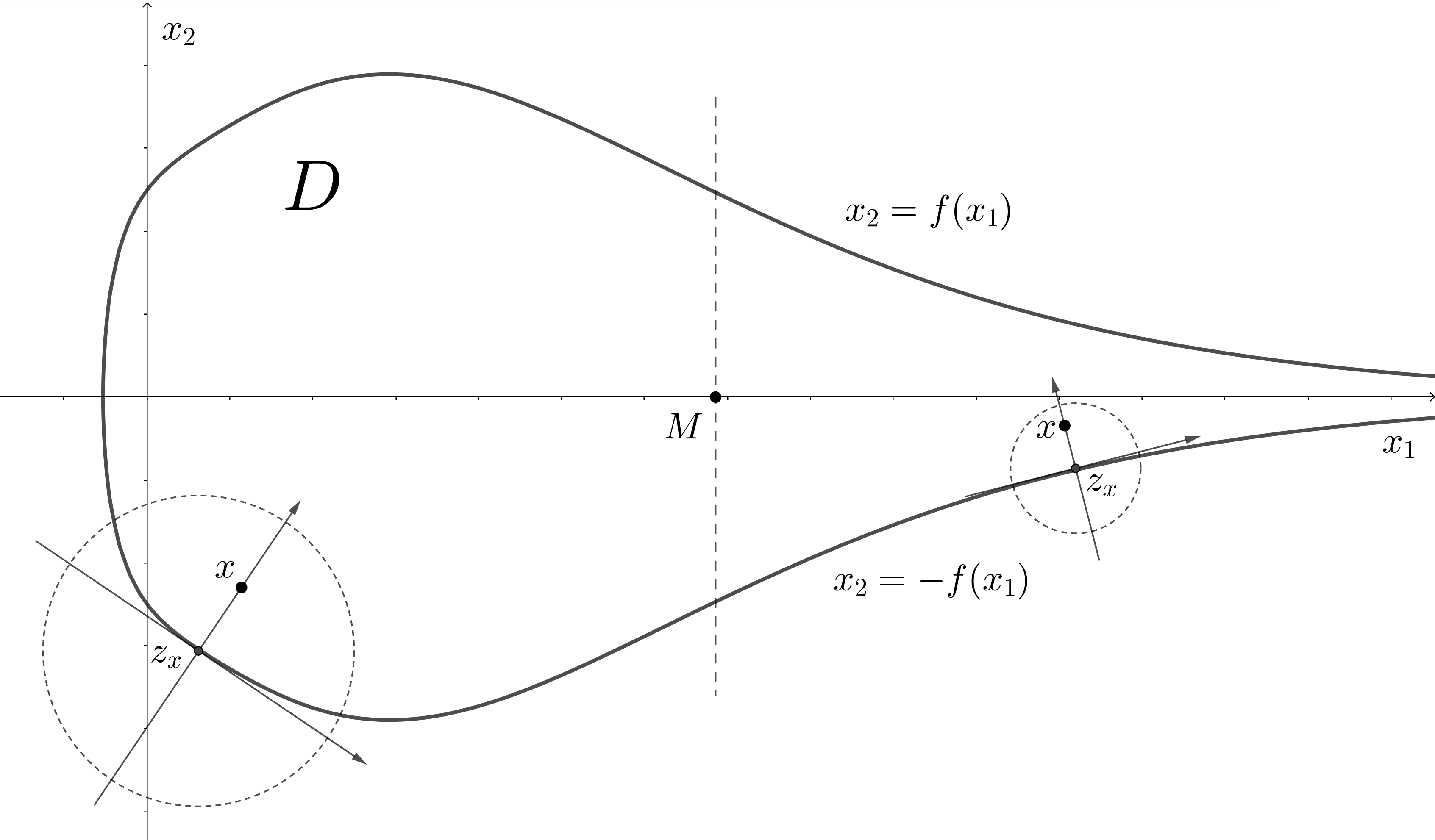
Figure 1. A horn-shaped $C^{1,1}$ region in $\mathds{R}^{2}$.

Remark 1.2.

It is easy to see that, for every horn-shaped region $D$ with the reference function $f$, there exist horn-shaped $C^{1,1}$ regions $U_{1}$ and $U_{2}$ with the same reference function $f$ such that $U_{1}\subset D\subset U_{2}$, and $\delta_{U_{1}}(x)=\delta_{U_{2}}(x)=\delta_{D}(x)$ for $x\in D^{M}_{f}$ with some constant $M>0$.

For both mathematical and physical backgrounds on the study of analytic properties related to horn-shaped regions, readers are referred to [1, 2, 3, 4, 8, 26, 28, 35]. We note that the properties (1.5)–(1.7) of the reference function $f$ essentially are also imposed in [1, 2, 3, 26, 28, 35], when explicit two-sided estimates for Dirichlet eigenfunctions for horn-shaped regions are concerned.

In the following, we fix a $C^{1,1}$ horn-shaped region $D$ with the reference function $f$, and set

$$\Psi(t,x):=\frac{\delta_{D}(x)^{\alpha/2}\left(f(x_{1})^{\alpha/2}\wedge t^{1/2}\right)}{t\wedge 1}\wedge 1,\quad x\in D,t>0.$$ (1.8)

The function $\Psi(t,x)$ will be used to describe the behavior of Dirichlet heat kernels near the boundary of $D$. Note that, by the definition of $D$, there exists a constant $c_{0}>0$ such that $\delta_{D}(x)\leqslant c_{0}f(x_{1})$ for all $x\in D$. Thus, there exist $c_{1},c_{2}>0$ such that for all $x\in D$ and $t>0$,

$$\Psi(t,x)\simeq \begin{cases}\displaystyle 1&\text{ if }\delta_{D}(x)\geqslant c_{1}t^{1/\alpha};\\ \displaystyle\frac{\delta_{D}(x)^{\alpha/2}}{\sqrt{t}}&\text{ if }\delta_{D}(x)\leqslant c_{1}t^{1/\alpha}\leqslant c_{2}f(x_{1});\\ \displaystyle\frac{\delta_{D}(x)^{\alpha/2}f(x_{1})^{\alpha/2}}{t\wedge 1}&\text{ if }c_{1}t^{1/\alpha}\geqslant c_{2}f(x_{1}).\end{cases}$$

We also set

$$\phi(x):=\frac{\delta_{D}(x)^{\alpha/2}f(x_{1})^{\alpha/2}}{(1+|x|)^{d+\alpha}},\quad x\in D,$$ (1.9)

which is comparable to the ground state of Dirichlet fractional Laplacian $(-\Delta)^{\alpha/2}|_{D}$ for the horn-shaped region $D$; see [34, Theorem 1 and Proposition 1] or [8, Theorem 6.1] for more details.

For any fixed constant $c>0$, let $t_{0}(x):=t_{0}(c,x)\in(0,\infty)$, which is defined for all $x\in D$, such that

$$e^{-ct_{0}(x)f(x_{1})^{-\alpha}}=t_{0}(x)(1+|x|)^{-(d+\alpha-1)},\quad x\in D.$$ (1.10)

Since the function $t\mapsto e^{-c_{0}f(x_{1})^{-\alpha}t}$ is continuous and strictly decreasing on $(0,\infty)$ with values on $(0,1)$ and the function $t\mapsto t(1+|x|)^{-(d+\alpha-1)}$ is continuous and strictly increasing on $(0,\infty)$ with values on $(0,\infty)$, $t_{0}(x)$ exists and is unique for all $x\in D$. The functions $e^{-c_{0}f(x_{1})^{-\alpha}t}$ and $t(1+|x|)^{-(d+\alpha-1)}$ come from estimates of the survival probability $\mathds{P}^{x}(\tau_{D}>t)$; see Lemma 2.8 below. One can see that there is a constant $c_{1}>0$ such that for all $x\in D$, $f(x_{1})^{\alpha}\leqslant c_{1}t_{0}(x).$ Usually it is not easy to obtain the explicit value of $t_{0}(x)$; however, we possibly can get explicit estimates of $t_{0}(x)$ for all $x\in D$ under some mild assumption on the reference function $f$. For example, if $f(r)\geqslant c(1+r)^{-p}$ for some constants $c$ and $p>0$, then $t_{0}(x)\simeq f(x_{1})^{\alpha}\log(2+|x|)$ for all $x\in D$.

The main result of this paper is as follows.

Theorem 1.3.

Suppose that $d\geqslant 2$ and $D$ is a $C^{1,1}$ horn-shaped region of $\mathds{R}^{d}$ associated with the reference function $f$ satisfying (1.5), (1.6) and (1.7). Let $p_{D}(t,x,y)$ be the transition density of killed symmetric $\alpha$-stable process $X^{D}$ with $\alpha\in(0,2)$. Then, there exist constants $c_{1.3.0},c_{1.3.1}>0$ such that the following two statements hold with $t_{0}(\cdot):=t_{0}(c_{1.3.0},\cdot)$.

(1) For any $x,y\in D$ and any $0<t\leqslant c_{1.3.1}(f(x_{1})\vee f(y_{1}))^{\alpha}\leqslant 1$,

$$p_{D}(t,x,y)\simeq p(t,x,y)\Psi(t,x)\Psi(t,y).$$ (1.11)

(2) Suppose in addition that $f(s)\geqslant c(1+s)^{-p}$ on $(0,\infty)$ for some $c,p>0$, and the function $s\mapsto f(s)^{\alpha}\log(2+s)$ is comparable to some monotone function $g$ on $(0,\infty)$ $($i.e. $g(s)\simeq f(s)^{\alpha}\log(2+s)$$)$.

• If $g$ is non-increasing on $(0,\infty)$ so that $\lim\limits_{s\to\infty}g(s)=0$, then there exist positive constants $c_{1.3.i}$ $(2\leqslant i\leqslant 10)$ such that for any $x,y\in D$ and any $c_{1.3.1}(f(x_{1})\vee f(y_{1}))^{\alpha}\leqslant t\leqslant c_{1.3.2}(t_{0}(x)\vee t_{0}(y))(\leqslant c_{1.3.2}\|t_{0}\|_{\infty}<\infty)$,

  $$\begin{split}\qquad p_{D}(t,x,y)\asymp p(t,x,y)\Psi(t,x)\Psi(t,y)\exp\left\{-t(f(x_{1})\vee f(y_{1}))^{-\alpha}\right\};\end{split}$$ (1.12)

  and for any $x,y\in D$ and any $t\geqslant c_{1.3.2}(t_{0}(x)\vee t_{0}(y))$,

  $$\begin{split}\qquad&c_{1.3.3}\phi(x)\phi(y)\max\Big{\{}\int_{0}^{c_{1.3.4}s_{1}(c_{1.3.5}t)}f(s)^{d-1}e^{-c_{1.3.6}tf(s)^{-\alpha}}\,ds,e^{-c_{1.3.6}t}\Big{\}}\\ \qquad&\leqslant p_{D}(t,x,y)\\ \qquad&\leqslant c_{1.3.7}\phi(x)\phi(y)\max\Big{\{}\int_{0}^{c_{1.3.8}s_{1}(c_{1.3.9}t)}f(s)^{d-1}e^{-c_{1.3.10}tf(s)^{-\alpha}}\,ds,e^{-c_{1.3.10}t}\Big{\}},\end{split}$$ (1.13)

  where $s_{1}(t)=g^{-1}(t)\vee 2$ and $g^{-1}(t)=\inf\{s\geqslant 0:g(s)\leqslant t\}$ for $t>0$.

• If $g$ is non-decreasing on $(0,\infty)$ so that $\lim\limits_{s\to\infty}g(s)>0$, then there exists a constant $c_{1.3.2}>0$ such that for any $x,y\in D$ and any $c_{1.3.1}((f(x_{1})\vee f(y_{1}))^{\alpha}\leqslant t\leqslant c_{1.3.2}(t_{0}(x)\wedge t_{0}(y))$,

  $$\qquad p_{D}(t,x,y)\asymp p(t,x,y)\Psi(t,x)\Psi(t,y)\exp\{-t(f(x_{1})\vee f(y_{1}))^{-\alpha}\};$$ (1.14)

  and for any $x,y\in D$ and any $t\geqslant c_{1.3.2}(t_{0}(x)\wedge t_{0}(y))(\geqslant c_{1.3.2}\inf_{z\in D}t_{0}(z)>0)$,

  $$\qquad p_{D}(t,x,y)\asymp\phi(x)\phi(y)e^{-t}.$$ (1.15)

Remark 1.4.

Let us give some remarks on Theorem 1.3.

(i) It is clear from Remark 1.2 and the proof of Theorem 1.3 that, for horn-shaped region $D$ (not necessarily $C^{1,1}$ near the origin), the conclusions of Theorem 1.3 still hold true for all $x,y\in D$ with $|x|\vee|y|$ large enough.

(ii) When $0<t\leqslant c_{1}(f(x_{1})^{\alpha}\wedge f(y_{1})^{\alpha})$, $p_{D}(t,x,y)$ satisfies (1.11), which is of the same form as (1.2); that is, $p_{D}(t,x,y)$ is comparable with the global heat kernel $p(t,x,y)$ multiplied by weighted functions $\Psi(t,x)$ and $\Psi(t,y)$, which are comparable to $\frac{\delta_{D}(x)^{\alpha/2}}{\sqrt{t}}\wedge 1$ and $\frac{\delta_{D}(y)^{\alpha/2}}{\sqrt{t}}\wedge 1$ respectively. This assertion is reasonable since $C^{1,1}$ horn-shaped region $D$ enjoys the “semi-uniform”  interior ball condition in the sense that for any $x\in D$ and $r\in(0,c_{*}f(x_{1}))$ (with possibly small $c_{*}$), $B(\xi_{x,r}^{*},r)\subset D$ with $\xi_{x,r}^{*}=z_{x}+r(x-z_{x})/|x-z_{x}|$.

(iii) For $t\geqslant c_{1}(f(x_{1})^{\alpha}\vee f(y_{1})^{\alpha})$, estimates for $p_{D}(t,x,y)$ heavily rely on the asymptotic property of the reference function $f$. According to [34, Theorem 5], under assumptions of case (i) in (2) the associated Dirichlet semigroup $(P_{t}^{D})_{t\geqslant 0}$ is intrinsically ultracontractive. Note that $s_{1}(t)=2$ for large $t$ under assumptions of case (i) in (2). Hence, similar to (1.3), the estimate indicated in (1.13) for $t\geqslant 1$ essentially is a direct consequence of the intrinsic ultracontractivity of $(P_{t}^{D})_{t\geqslant 0}$. However, when $c_{1}(f(x_{1})^{\alpha}\vee f(y_{1})^{\alpha})\leqslant t\leqslant 1$, estimates for $p_{D}(t,x,y)$ are much more delicate.

(iv) It will be shown in Lemma 2.8 that the following upper bound on survival probability holds true: for any $x\in D$ and $t>0$,

$$\mathds{P}^{x}(\tau_{D}>t)\leqslant c_{1}\Psi(t,x)\min\Big{\{}e^{-c_{2}f(x_{1})^{-\alpha}t}+t(1+|x|)^{-(d+\alpha-1)},e^{-c_{2}t}\Big{\}}.$$ (1.16)

In particular, when $t=T_{0}:=c_{1.3.2}\|t_{0}\|_{\infty}<\infty$ and $10T_{0}<|x|\leqslant 2|y|$, (1.16) implies that

$$p(T_{0},x,y)\mathds{P}^{x}(\tau_{D}>T_{0})\mathds{P}^{y}(\tau_{D}>T_{0})\leqslant c_{3}(T_{0})\frac{\phi(x)\phi(y)|x|}{|y|^{d+\alpha-1}}.$$

On the other hand, (1.13) implies that $p_{D}(T_{0},x,y)\asymp\phi(x)\phi(y)$. Therefore, the so-called Varopoulos-type estimates (1.4) do not hold true under assumptions of case (i) in (2), which is different from [11, Theorem 1.1] and [6, Theorem 1].

(v) Under assumptions of case (ii) in (2), the associated Dirichlet semigroup $(P^{D}_{t})_{t\geqslant 0}$ is not intrinsically ultracontractive, see also [34, Theorem 5]. Though (1.14) is of the same form as that for (1.12), the ranges of time variable are different; that is, $c_{2}(t_{0}(x)\wedge t_{0}(y))\geqslant 1$ in (1.14), while $c_{2}(t_{0}(x)\vee t_{0}(y))\leqslant 1$ in (1.12). Also by this reason, the estimates (1.13) and (1.15) are different too, even both of them enjoy the same form (by neglecting constants in the exponential term) when $t\to\infty$.

The proof of Theorem 1.3 is completely different from those in [11] and [24], where two-sided Dirichlet heat kernel estimates for fractional Laplacians in uniformly $C^{1,1}$ open sets and half-space-like open sets were established respectively. For example, because of the non-uniformity on $C^{1,1}$ characteristics, the boundary Harnack principle can not be applied to $C^{1,1}$ horn-shaped regions, and so the approach of [11, Theorem 1.1 (i)] does not work in the present setting. In order to obtain Dirichlet heat kernel estimates of horn-shaped regions, we need to take into accounts carefully the interaction between jumping kernel of symmetric $\alpha$-stable processes and the characterization (heavily depending on the reference function $f$) of the horn-shaped region. Roughly speaking, the proof of Theorem 1.3 is split into three cases according to different ranges of time and space. (1) When $0<t\leqslant c_{1}(f(x_{1})\vee f(y_{1}))^{\alpha}$, we make use of the Chapman-Kolmogorov equation and a general formula for upper bounds of Dirichlet heat kernels (see [7, Lemma 1.10], [29, Lemma 5.1] and [20, Lemma 3.1]). Note that, in this case the estimates for exit probability (see Lemma 2.6) are different from those implied by (1.2) when $c_{1}(f(x_{1})\wedge f(y_{1}))^{\alpha}\leqslant t\leqslant c_{1}(f(x_{1})\vee f(y_{1}))^{\alpha}$. (2) When $c_{1}(f(x_{1})\vee f(y_{1}))^{\alpha}\leqslant t\leqslant c_{2}(t_{0}(x)\vee t_{0}(y))$ or $c_{1}(f(x_{1})\vee f(y_{1}))^{\alpha}\leqslant t\leqslant c_{2}(t_{0}(x)\wedge t_{0}(y))$, we will adopt the chain argument to derive lower bounds and apply the split technique combined with the survival probability (2.10) to obtain upper bounds. In particular, in arguments for both cases above, instead of the boundary Harnack principle, we make use of the Lévy system. (3) When $t\geqslant c_{2}(t_{0}(x)\vee t_{0}(y))$ or $t\geqslant c_{2}(t_{0}(x)\wedge t_{0}(y))$, the dominant behaviour (with the largest probability) of the killed process taking time $t$ from $x$ to $y$ is that, the process jumps form $x$ to the origin, and then jumps to $y$ after spending more than $t/2$ at a neighborhood of origin or at another neighborhood inside $D$ with the largest survival probability. This gives us the intuitive meanings of (1.13) and (1.15). In this case, lower bounds are derived by using assertions in cases (1) and (2); however, the proofs of upper bounds are much more involved. In particular, we will use the iteration arguments based on the survival probability.

1.2. Relation with intrinsic ultracontractivity

Recall that in the present setting the Dirichlet semigroup $(P^{D}_{t})_{t\geqslant 0}$ is intrinsically ultracontractive, if for every $t>0$ there is a constant $C_{D,t}>0$ such that

$$p_{D}(t,x,y)\leqslant C_{D,t}\phi(x)\phi(y),\quad x,y\in D,$$ (1.17)

where $\phi$ is defined by (1.9) that is comparable with the ground state of $(P^{D}_{t})_{t\geqslant 0}$.

The intrinsic ultracontractivity of Markov semigroups (including Dirichlet semigroups and Feyman-Kac semigroups) has been intensively established for various Lévy type processes. For more details, see [9, 10] and the references therein. The intrinsic ultracontractivity and two-sided estimates of ground state for symmetric $\alpha$-stable processes and more general symmetric jump processes on unbounded open sets were investigated in [34] and [8], respectively. We note that the two-sided Dirichlet heat kernel estimates are much more complex than estimates of ground state. Informally, to obtain Dirichlet heat kernel estimates we need to consider the relationship between time and space carefully; for ground state estimates we only just take time $t=1$ and make use of estimates for $p(1,x,y)$; see [8, Sections 5 and 6].

In the following, we deduce explicit estimates for the intrinsic ultracontractivity under assumptions in (i) of (2) in Theorem 1.3, by directly applying two-sided Dirichlet heat kernel estimates. Recall that $g(s)\simeq f(s)^{\alpha}\log(2+s)$.

Proposition 1.5.

Under assumptions in (i) of (2) in Theorem 1.3, (1.17) holds with

$$C_{D,t}=c_{1.5.{2}}\begin{cases}\displaystyle t^{-2-d/\alpha}(1+g^{-1}(c_{1.5.{3}}t))^{2d+2\alpha},&\,\,0<t\leqslant c_{1.5.{1}}(t_{0}(x)\vee t_{0}(y));\\ \displaystyle\max\Big{\{}\int_{0}^{c_{1.5.{4}}s_{1}(c_{1.5.{5}}t)}f(s)^{d-1}e^{-c_{1.5.{6}}tf(s)^{-\alpha}}\,ds,e^{-c_{1.5.{7}}t}\Big{\}},&\,\,t>c_{1.5.{1}}(t_{0}(x)\vee t_{0}(y)).\end{cases}$$

Proof.

According to (1.11) and (1.12), there are constants $c_{0},c_{1}>0$ such that $p_{D}(t,x,y)\leqslant c_{1}p(t,x,y)\Psi(t,x)\Psi(t,y)$ for any $x,y\in D$ and $0<t\leqslant c_{0}(t_{0}(x)\vee t_{0}(y))\leqslant 1$.

In the following, without loss of generality, we may assume that $x,y\in D$ with $x_{1}\geqslant y_{1}$. According to the non-increasing property of the function $g$ and $\lim_{s\to\infty}g(s)=0$ as well as $t_{0}(y)\simeq g(|y|)$, $t\leqslant c_{2}t_{0}(y)$ for some $c_{2}>0$ implies that $|y|\leqslant c_{3}g^{-1}(c_{4}t)$. In particular,

$$(1+|y|)^{d+\alpha}\leqslant\left(1+c_{3}g^{-1}(c_{4}t)\right)^{d+\alpha}.$$ (1.18)

Thus, if $|y|/2\leqslant|x|\leqslant 2|y|$, then, for $0<t\leqslant c_{0}(t_{0}(x)\vee t_{0}(y))\leqslant 1$,

$$p_{D}(t,x,y)\leqslant c_{5}t^{-d/\alpha}\frac{\delta_{D}(x)^{\alpha/2}(f(x_{1})^{\alpha/2}\wedge t^{1/2})}{t}\frac{\delta_{D}(y)^{\alpha/2}(f(y_{1})^{\alpha/2}\wedge t^{1/2})}{t}$$

$$\leqslant c_{6}t^{-2-d/\alpha}(1+g^{-1}(c_{7}t))^{2d+2\alpha}\frac{\delta_{D}(x)^{\alpha/2}f(x_{1})^{\alpha/2}}{(1+|x|)^{d+\alpha}}\frac{\delta_{D}(y)^{\alpha/2}f(y_{1})^{\alpha/2}}{(1+|y|)^{d+\alpha}}$$

$$= c_{6}t^{-2-d/\alpha}(1+g^{-1}(c_{7}t))^{2d+2\alpha}\phi(x)\phi(y),$$

where in the second inequality we used the fact that $|y|/2\leqslant|x|\leqslant 2|y|$ and (1.18); if $|x|\geqslant 2|y|$, then, for $0<t\leqslant c_{0}(t_{0}(x)\vee t_{0}(y))$, we can argue as follows

$$p_{D}(t,x,y)\leqslant \frac{c_{8}t}{(1+|x|)^{d+\alpha}}\frac{\delta_{D}(x)^{\alpha/2}(f(x_{1})^{\alpha/2}\wedge t^{1/2})}{t}\frac{\delta_{D}(y)^{\alpha/2}(f(y_{1})^{\alpha/2}\wedge t^{1/2})}{t}$$

$$\leqslant c_{9}t^{-1}(1+g^{-1}(c_{10}t))^{d+\alpha}\frac{\delta_{D}(x)^{\alpha/2}f(x_{1})^{\alpha/2}}{(1+|x|)^{d+\alpha}}\frac{\delta_{D}(y)^{\alpha/2}f(y_{1})^{\alpha/2}}{(1+|y|)^{d+\alpha}}$$

$$= c_{9}t^{-1}(1+g^{-1}(c_{10}t))^{d+\alpha}\phi(x)\phi(y),$$

where the first inequality follows from the fact that $|x|\geqslant 2|y|$, and the second inequality is due to (1.18). Similarly, we can prove that if $|x|\leqslant|y|/2$, then, for $0<t\leqslant c_{0}(t_{0}(x)\vee t_{0}(y))$,

$$p_{D}(t,x,y)\leqslant c_{11}t^{-1}(1+g^{-1}(c_{12}t))^{d+\alpha}\phi(x)\phi(y).$$

Combining all the estimates above with (1.13), we can obtain that (1.17) holds for all $x,y\in D$ and $t>0$ with the desired estimates for $C_{D,t}$. ∎

We would like to mention that the arguments above (in particular, (1.18)) fail, under assumptions in (ii) of (2) in Theorem 1.3, i.e., when the function $g(s)$ is non-decreasing on $(0,\infty)$.

1.3. A toy example

In this part, we present the following example to illustrate how powerful Theorem 1.3 is.

Example 1.6.

Let $f(s)=\log^{-\theta}(2+s)$ with $\theta>0$ for all $s\in[0,\infty)$. For any $x,y\in D$, set $t_{1}(x,y)=\log^{-\theta\alpha}(e+(|x|\wedge|y|))$ and $t_{2}(x,y)=\log^{-(\theta\alpha-1)}(e+(|x|\wedge|y|)).$ Then, we have the following two statements.

(i) Assume that $\theta>1/\alpha$. Then, there exist positive constants $c_{1.6.1}$, $c_{1.6.2}$ and $c_{1.6.3}$ such that for all $x,y\in D$,

$$p_{D}(t,x,y)\asymp$$

$$\begin{cases}\displaystyle p(t,x,y)\bigg{(}\frac{\delta_{D}(x)^{\alpha/2}\left(\log^{-\theta\alpha/2}(e+|x|)\wedge t^{1/2}\right)}{t}\wedge 1\bigg{)}\bigg{(}\frac{\delta_{D}(y)^{\alpha/2}\left(\log^{-\theta\alpha/2}(e+|y|)\wedge t^{1/2}\right)}{t}\wedge 1\bigg{)}\\ \qquad\qquad\qquad\qquad\qquad\qquad\qquad\qquad\qquad\qquad\qquad\qquad\text{for all }0<t\leqslant c_{1.6.1}t_{1}(x,y);\\[2.0pt] \displaystyle p(t,x,y)\frac{\delta_{D}(x)^{\alpha/2}\log^{-\theta\alpha/2}(e+|x|)}{t}\frac{\delta_{D}(y)^{\alpha/2}\log^{-\theta\alpha/2}(e+|y|)}{t}\exp(-t\log^{\theta\alpha}(e+(|x|\wedge|y|)))&\\ \qquad\qquad\qquad\qquad\qquad\qquad\qquad\qquad\qquad\qquad\qquad\qquad\text{for all }c_{1.6.1}t_{1}(x,y)<t\leqslant c_{1.6.2}t_{2}(x,y);\\[2.0pt] \displaystyle\frac{\delta_{D}(x)^{\alpha/2}\log^{-\theta\alpha/2}(e+|x|)}{(1+|x|)^{d+\alpha}}\frac{\delta_{D}(y)^{\alpha/2}\log^{-\theta\alpha/2}(e+|y|)}{(1+|y|)^{d+\alpha}}\exp(t^{-1/(\theta\alpha-1)}),&\\ \qquad\qquad\qquad\qquad\qquad\qquad\qquad\qquad\qquad\qquad\qquad\qquad\text{for all }c_{1.6.2}t_{2}(x,y)<t\leqslant c_{1.6.3};\\[2.0pt] \displaystyle\frac{\delta_{D}(x)^{\alpha/2}\log^{-\theta\alpha/2}(e+|x|)}{(1+|x|)^{d+\alpha}}\frac{\delta_{D}(y)^{\alpha/2}\log^{-\theta\alpha/2}(e+|y|)}{(1+|y|)^{d+\alpha}}\exp(-t),\\ \qquad\qquad\qquad\qquad\qquad\qquad\qquad\qquad\qquad\qquad\qquad\qquad\text{for all }t>c_{1.6.3}.\end{cases}$$

(ii) Assume that $\theta\leqslant 1/\alpha$. Then, there exist positive constants $c_{1.6.4}$ and $c_{1.6.5}$ such that for all $x,y\in D$,

$$p_{D}(t,x,y)\asymp$$

$$\begin{cases}\displaystyle\bigg{(}\frac{\delta_{D}(x)^{\alpha/2}\left(\log^{-\theta\alpha/2}(e+|x|)\wedge t^{1/2}\right)}{t}\wedge 1\bigg{)}\bigg{(}\frac{\delta_{D}(y)^{\alpha/2}\left(\log^{-\theta\alpha/2}(e+|y|)\wedge t^{1/2}\right)}{t}\wedge 1\bigg{)}\\ \qquad\qquad\qquad\qquad\qquad\qquad\qquad\qquad\qquad\qquad\qquad\qquad\text{for all }0<t\leqslant c_{1.6.4}t_{1}(x,y);\\[2.0pt] \displaystyle p(t,x,y)\frac{\delta_{D}(x)^{\alpha/2}\log^{-\theta\alpha/2}(e+|x|)}{t}\frac{\delta_{D}(y)^{\alpha/2}\log^{-\theta\alpha/2}(e+|y|)}{t}\exp\big{(}-t\log^{\theta\alpha}(e+(|x|\wedge|y|))\big{)}\\ \qquad\qquad\qquad\qquad\qquad\qquad\qquad\qquad\qquad\qquad\qquad\qquad\text{for all }c_{1.6.4}t_{1}(x,y)<t\leqslant c_{1.6.5}t_{2}(x,y);\\[2.0pt] \displaystyle\frac{\delta_{D}(x)^{\alpha/2}\log^{-\theta\alpha/2}(e+|x|)}{(1+|x|)^{d+\alpha}}\frac{\delta_{D}(y)^{\alpha/2}\log^{-\theta\alpha/2}(e+|y|)}{(1+|y|)^{d+\alpha}}\exp(-t)\\ \qquad\qquad\qquad\qquad\qquad\qquad\qquad\qquad\qquad\qquad\qquad\qquad\text{for all }t>c_{1.6.5}t_{2}(x,y).\end{cases}$$

Proof.

This directly follows from Theorem 1.3. Here we give some details on the case that $\theta>1/\alpha$ and $c_{1.6.2}t_{2}(x,y)\leqslant t\leqslant c_{1.6.3}$. For any $t>0$, define

$$s_{1}(t)=\inf\{s>0:f(s)^{\alpha}\log(2+s)\leqslant t\}\vee 2.$$

Then, for $0<t\leqslant 1$,

$$s_{1}(t)\asymp\exp\big{(}{t^{-1/(\theta\alpha-1)}}\big{)}.$$

Hence, for any $c_{i}>0$ $(1\leqslant i\leqslant 3)$ and $t\in(0,1]$,

$$\int_{0}^{c_{1}s_{1}(c_{2}t)}f(s)^{d-1}e^{-c_{3}tf(s)^{-\alpha}}\,ds\asymp\exp\big{(}{t^{-1/(\theta\alpha-1)}}\big{)}.$$

Indeed, it is clear that for all $t\in(0,1]$,

$$\int_{0}^{c_{1}s_{1}(c_{2}t)}f(s)^{d-1}e^{-c_{3}tf(s)^{-\alpha}}\,ds\leqslant(\log 2)^{-\theta(d-1)}\int_{0}^{c_{1}s_{1}(c_{2}t)}\,ds\leqslant c_{4}\exp({c_{5}t^{-1/(\theta\alpha-1)}}).$$

On the other hand, noting that $c_{1}s_{1}(c_{2}t)\geqslant c_{6}\exp({c_{7}t^{-1/(\theta\alpha-1)}})$ for all $t\in(0,1]$ with some $c_{6},c_{7}>0$ that satisfies $2c_{3}c_{7}^{\theta\alpha-1}\leqslant 1$, and also that the function $s\mapsto f(s)^{d-1}e^{-c_{3}tf(s)^{-\alpha}}$ is decreasing on $(0,\infty)$, we have

$$\int_{0}^{c_{1}s_{1}(c_{2}t)}f(s)^{d-1}e^{-c_{3}tf(s)^{-\alpha}}\,ds$$

$$\geqslant\int_{0}^{c_{6}\exp({c_{7}t^{-1/(\theta\alpha-1)}})}f(s)^{d-1}e^{-c_{3}tf(s)^{-\alpha}}\,ds$$

$$\geqslant\log^{-\theta(d-1)}\left(2+c_{6}\exp({c_{7}t^{-1/(\theta\alpha-1)}})\right)\cdot\exp\left(-c_{3}t\log^{\alpha\theta}(2+c_{6}e^{c_{7}t^{-1/(\theta\alpha-1)}})\right)\cdot c_{6}\exp({c_{7}t^{-1/(\theta\alpha-1)}})$$

$$\geqslant c_{8}t^{\theta(d-1)/(\theta\alpha-1)}\exp(-c_{9}t-c_{3}c_{7}^{\theta\alpha}t^{-1/(\theta\alpha-1)})\cdot\exp({c_{7}t^{-1/(\theta\alpha-1)}})$$

$$\geqslant c_{10}t^{\theta(d-1)/(\theta\alpha-1)}\exp\left({\frac{c_{7}}{2}t^{-1/(\theta\alpha-1)}}\right)\geqslant\exp({c_{11}t^{-1/(\theta\alpha-1)}})$$

for all $t\in(0,1]$.

With these at hand, we can get the required assertions in Example 1.6. ∎

Note that, for this example, the associated Dirichlet semigroup $(P^{D}_{t})_{t\geqslant 0}$ is intrinsically ultracontractive, if and only if $\theta>1/\alpha$; see [34, Example 2] or [8, Theorem 1.1(1)]. On the other hand, it is easy to see that $\limsup_{|x|,|y|\to\infty}t_{2}(x,y)=0$, if and only if $\theta>1/\alpha$. This explains why there is a threshold at $\theta=1/\alpha$ for two-sided estimates of $p_{D}(t,x,y)$.

The rest of this paper is arranged as follows. The next section serves as preparations for main proofs. Results in Sections 2 will be frequently used in the proof of Theorem 1.3. In particular, upper bound estimates of survival probabilities for full time are presented here. Sections 3, 4 and 5 are devoted to the proof of Theorem 1.3, according to different ranges of time. Proof of Theorem 1.3 and further remarks are briefly given in Section 6.

2. Preparations

2.1. Preliminary estimates

In this part, we collect some (mostly known) results which will be frequently used in proofs of our paper. Throughout this paper, let $X:=\{X_{t},t\geqslant 0;\mathds{P}^{x},x\in\mathds{R}^{d}\}$ be a (rotationally) symmetric $\alpha$-stable process in $\mathds{R}^{d}$ with $d\geqslant 2$, whose transition density is denoted by $p(t,x,y)$. For any open subset $U$, let $X^{U}$ be the subprocess of $X$ killed upon leaving $U$, whose transition density is denoted by $p_{U}(t,x,y)$. Let $\tau_{U}:=\inf\{t\geqslant 0:X_{t}\notin U\}$ be the first exit time from $U$ for the process $X$. It is well known (cf. see [11, Lemma 3.2]) that, for any $\kappa_{1},\kappa_{2}>0$, there exists a constant $c_{1}:=c_{1}(\kappa_{1},\kappa_{2})>0$ such that for all $x\in\mathds{R}^{d}$ and $t>0$,

$$\mathds{P}^{x}\left(\tau_{B(x,\kappa_{1}t^{1/\alpha})}>\kappa_{2}t\right)\geqslant c_{1}.$$ (2.1)

Recall that the Lévy system of $X$ describes the behaviors of jumps for the process $X$. In particular, given a non-negative function $f:\mathds{R}_{+}\times\mathds{R}^{d}\times\mathds{R}^{d}\to\mathds{R}_{+}$ with $f(s,x,x)=0$ for all $s>0$ and $x\in\mathds{R}^{d}$, it holds for any stopping time $\tau$ that

$$\mathds{E}^{x}\left[\sum_{s\leqslant\tau}f\left(s,X_{s-},X_{s}\right)\right]=\mathds{E}^{x}\int_{0}^{\tau}\int_{\mathds{R}^{d}}f\left(s,X_{s},y\right)\frac{c_{d,\alpha}}{|X_{s}-y|^{d+\alpha}}\,dy\,ds.$$ (2.2)

We refer the reader to [22, Lemma 4.7] for more details about the property of Lévy system. On the other hand, according to [34, Lemma 2], we have

Lemma 2.1.

There exists a constant $c_{2.1.{1}}\!>0$ such that for any open set $U\subset\mathds{R}^{d}$, $x\in U$ and $t>0$,

$$\mathds{P}^{x}\left(\tau_{U}>t\right)\leqslant\exp\left(-c_{2.1.{1}}\eta_{U}t\right),$$ (2.3)

where $\eta_{U}:=\inf_{x\in U}\displaystyle\int_{U^{c}}{|x-z|^{-d-\alpha}\,}dz.$

Throughout the remainder of this paper, let $f:\mathds{R}\to(0,\infty)$ satisfy (1.5), (1.6) and (1.7). For fixed constants $c_{*}\in(0,1/5]$ and $\Lambda>0$, let $D$ be a horn-shaped $C^{1,1}$ region with the reference function $f$ so that for all $x\in D$, $D$ is $C^{1,1}$ at $z_{x}\in\partial D$ with the characteristics $(5c_{*}f(x_{1}),\Lambda)$.

To save notations in the proofs, without loss of generality, we may assume that the following conditions are satisfied:

(i) $f(0)\leqslant 2^{-2}$, and for all $x\in D$, $\delta_{D}(x)\leqslant 2^{-1}$;

(ii) $D\cap\{x\in\mathds{R}^{d}:x_{1}<2\}\subset B(0,2)$, and $\{x\in D:x_{1}>2\}=D^{2}_{f}$;

(iii)(non-uniform) Interior ball condition:  for every $x\in D$ and $0<r\leqslant 5c_{*}f(x_{1})$, $B(\xi^{*}_{x,r},r)\subset D$, where $\xi^{*}_{x,r}:=z_{x}+r({x-z_{x}})/{|x-z_{x}|}$.

We remark here that, clearly the arguments below work for general $C^{1,1}$ horn-shape regions without the additional assumptions (i)–(iii).

Lemma 2.2.

There exists a constant $c_{2.2.{1}}>0$ such that for all $x\in D$, $0<t\leqslant c_{2.2.{1}}f(x_{1})^{\alpha}$ and $\lambda_{i}>0$ $(i=1,2,3)$, there is a constant $c_{2.2.{2}}:=c_{2.2.{2}}(c_{2.2.{1}},\lambda_{1},\lambda_{2},\lambda_{3})$ so that when $\delta_{D}(x)\geqslant\lambda_{1}t^{1/\alpha}$, $p_{D}(t,x,y)\geqslant c_{2.2.{2}}t^{-d/\alpha}$ holds for all $y\in D$ with $\delta_{D}(y)\geqslant\lambda_{2}t^{1/\alpha}$ and $|x-y|\leqslant\lambda_{3}t^{1/\alpha}$.

Proof.

Since for any $x\in D$, $D$ is $C^{1,1}$ at $z_{x}\in\partial D$ with the characteristics $(5c_{*}f(x_{1}),\Lambda)$, the desired assertion can be proven by the arguments for the proof of [11, Proposition 3.3] or [19, Proposition 3.6]. ∎

The next lemma is partially motivated by [32, Lemma 5.4] and [29, Lemma 7.4].

Lemma 2.3.

For every $\lambda\in(0,1]$, there exists a constant $c_{2.3.{1}}:=c_{2.3.{1}}(\lambda)>0$ such that for all $t>0$ and $x\in D$ with $0<t^{1/\alpha}\leqslant c_{*}f(x_{1})$, there is $\xi^{t}_{x}\in D$ so that $B(\xi^{t}_{x},4\lambda t^{1/\alpha})\subset D$ and

$$\int_{B(\xi^{t}_{x},2\lambda t^{1/\alpha})}p_{D}(t,x,z)\,dz\geqslant c_{2.3.{1}}\left(\frac{\delta_{D}(x)^{\alpha/2}}{\sqrt{t}}\wedge 1\right),$$ (2.4)

where

$$\xi_{x}^{t}:=\begin{cases}\xi^{*}_{x,4\lambda t^{1/\alpha}}=z_{x}+4\lambda t^{1/\alpha}({x-z_{x}})/{|x-z_{x}|}&\text{ when }\delta_{D}(x)\leqslant 4\lambda t^{1/\alpha};\\ x&\text{ when }\delta_{D}(x)>4\lambda t^{1/\alpha}.\end{cases}$$

Proof.

Fix $\lambda\in(0,1]$. If $\delta_{D}(x)>4\lambda t^{1/\alpha}$, then $B(x,4\lambda t^{1/\alpha})\subset D$, and so

$$\int_{B(x,2\lambda t^{1/\alpha})}p_{D}(t,x,z)\,dz \geqslant\int_{B(x,2\lambda t^{1/\alpha})}p_{B(x,2\lambda t^{1/\alpha})}(t,x,z)\,dz=\mathds{P}^{x}\big{(}\tau_{B(x,2\lambda t^{1/\alpha})}>t\big{)}\geqslant c_{4},$$

where the last inequality follows from (2.1) with $\kappa_{1}=2\lambda$ and $\kappa_{2}=1$. Thus (2.4) holds for this case.

Now, we turn to the case that $\delta_{D}(x)\leqslant 4\lambda t^{1/\alpha}$. Since $5\lambda t^{1/\alpha}\leqslant 5c_{*}f(x_{1})$, according to the (non-uniform) interior ball condition of $D$, $B(\xi^{t}_{x},4\lambda t^{1/\alpha})\subset D$ and $B(\tilde{\xi}^{t}_{x},5\lambda t^{1/\alpha})\subset D$ with $\tilde{\xi}^{t}_{x}:=\xi^{*}_{x,5\lambda t^{1/\alpha}}=z_{x}+5\lambda t^{1/\alpha}{x-z_{x}}/{|x-z_{x}|}.$ In particular, $B(\xi^{t}_{x},2\lambda t^{1/\alpha})\subset B(\tilde{\xi}^{t}_{x},5\lambda t^{1/\alpha})\subset D$. Since $\delta_{D}(x)\leqslant 4\lambda t^{1/\alpha}$, we have $x\in B(\tilde{\xi}^{t}_{x},5\lambda t^{1/\alpha})$ with $\delta_{B(\tilde{\xi}^{t}_{x},5\lambda t^{1/\alpha})}(x)=\delta_{D}(x)$, and, for any $z\in B(\xi^{t}_{x},2\lambda t^{1/\alpha})$, $|x-z|\leqslant|x-\xi^{t}_{x}|+|\xi^{t}_{x}-z|\leqslant c_{1}t^{1/\alpha}$ and $\delta_{B(\tilde{\xi}^{t}_{x},5\lambda t^{1/\alpha})}(z)\geqslant 2\lambda t^{1/\alpha}$. Thus, according to (1.2),

$$\int_{B(\xi^{t}_{x},2\lambda t^{1/\alpha})}p_{D}(t,x,z)\,dz\geqslant\int_{B(\xi^{t}_{x},2\lambda t^{1/\alpha})}p_{B(\tilde{\xi}^{t}_{x},5\lambda t^{1/\alpha})}(t,x,z)\,dz$$

$$\geqslant c_{2}\frac{\delta_{B(\tilde{\xi}^{t}_{x},5\lambda t^{1/\alpha})}(x)^{\alpha/2}}{\sqrt{t}}t^{-d/\alpha}\int_{B(\xi^{t}_{x},2\lambda t^{1/\alpha})}\frac{\delta_{B(\tilde{\xi}^{t}_{x},5\lambda t^{1/\alpha})}(z)^{\alpha/2}}{\sqrt{t}}\,dz\geqslant c_{3}\frac{\delta_{D}(x)^{\alpha/2}}{\sqrt{t}}.$$

∎

Lemma 2.4.

There exist constants $c_{2.4.{1}}\in(0,1)$ and $c_{2.4.{2}}>0$ such that for all $t>0$ and $x\in D$ with $0<t\leqslant c_{2.4.{1}}f(x_{1})^{\alpha}$,

$$\mathds{P}^{x}\big{(}\tau_{D}>t\big{)}\leqslant c_{2.4.{2}}\left(\frac{\delta_{D}(x)^{\alpha/2}}{\sqrt{t}}\wedge 1\right).$$ (2.5)

Proof.

It suffices to prove (2.5) for the case $\delta_{D}(x)\leqslant c_{1}t^{1/\alpha}$ with arbitrary fixed $c_{1}>0$.

On the one hand, note that for any $x\in D$, $D$ is $C^{1,1}$ at $z_{x}\in\partial D$ with the characteristics $(5c_{*}f(x_{1}),\Lambda)$. We can follow the proof of [32, (2.11) in Theorem 2.6] to find constants $c_{2},c_{3}\in(0,1)$ such that for every $x\in D$ and $0<t\leqslant c_{2}f(x_{1})^{\alpha}$ with $\delta_{D}(x)\leqslant c_{3}t^{1/\alpha}$,

$$\mathds{E}^{x}[\tau_{V_{t}}]\leqslant c_{4}t^{1/2}\delta_{D}(x)^{\alpha/2},$$ (2.6)

where $V_{t}:=B(z_{x},2c_{3}t^{1/\alpha})\cap D$.

On the other hand, according to [21, Lemma 2.4], it holds that for every $t>0$ and $x\in D$ with with $\delta_{D}(x)\leqslant c_{3}t^{1/\alpha}$,

$$\mathds{P}^{x}(X_{\tau_{V_{t}}}\in D)\leqslant\mathds{P}^{x}(X_{\tau_{V_{t}}}\in B(z_{x},2c_{3}t^{1/\alpha})^{c})\leqslant c_{5}t^{-1}\mathds{E}^{x}[\tau_{V_{t}}].$$ (2.7)

Combining both estimates above together yields that, for any $x\in D$ and $0<t\leqslant c_{2}f(x_{1})^{\alpha}$ with $\delta_{D}(x)\leqslant c_{3}t^{1/\alpha}$, (by noting that $f\leqslant 2^{-2}$),

$$\mathds{P}^{x}(\tau_{D}>t) =\mathds{P}^{x}(\tau_{V_{t}}\geqslant t)+\mathds{P}^{x}(\tau_{D}>t>\tau_{V_{t}})\leqslant\mathds{P}^{x}(\tau_{V_{t}}\geqslant t)+\mathds{P}^{x}(X_{\tau_{V_{t}}}\in D)$$

$$\leqslant c_{6}t^{-1}\mathds{E}^{x}[\tau_{V_{t}}]\leqslant c_{7}\frac{\delta_{D}(x)^{\alpha/2}}{\sqrt{t}},$$

proving the desired assertion. ∎

Lemma 2.5.

For all $\lambda\in(0,1]$, there exist constants $c_{2.5.{1}}:=c_{2.5.{1}}(\lambda)$ and $c_{2.5.{2}}:=c_{2.5.{2}}(\lambda)\in(0,1)$ such that for any $t>0$ and $x\in D$ with $0<t\leqslant c_{2.5.{1}}f(x_{1})^{\alpha}$ and $\delta_{D}(x)\leqslant\lambda t^{1/\alpha}$,

$$\mathds{P}^{x}\big{(}\tau_{B(z_{x},10\lambda t^{1/\alpha})\cap D}>t\big{)}\geqslant c_{2.5.{2}}\frac{\delta_{D}(x)^{\alpha/2}}{\sqrt{t}}.$$ (2.8)

Proof.

This follows from the proof of [32, Lemma 5.2], thanks to the fact that for any $x\in D$, $D$ is $C^{1,1}$ at $z_{x}\in\partial D$ with the characteristics $(5c_{*}f(x_{1}),\Lambda)$. ∎

Lemma 2.6.

There exist constants $c_{2.6.{1}}\in(0,1)$ and $c_{2.6.{2}}>0$ such that for all $t>0$ and $x\in D$ with $\delta_{D}(x)\leqslant c_{2.6.{1}}t^{1/\alpha}$,

$$\mathds{E}^{x}\big{[}\tau_{B(z_{x},c_{2.6.1}(t^{1/\alpha}\wedge 1))\cap D}\big{]}\leqslant c_{2.6.{2}}\delta_{D}(x)^{\alpha/2}\big{(}f(x_{1})^{\alpha/2}\wedge t^{1/2}\big{)}.$$ (2.9)

Proof.

Let $c_{2},c_{3}\in(0,1]$ be the constants in (2.6), and set $c_{2.6.{1}}=c_{3}$. When $0<t\leqslant c_{2}f(x_{1})^{\alpha}$, (2.9) follows from (2.6). If $t>c_{2}f(x_{1})^{\alpha}$, then, according to [8, Lemma 6.2] (by choosing $c_{2.6.{1}}$ small if necessary),

$$\mathds{E}^{x}\big{[}\tau_{B(z_{x},c_{2.6.{1}}(t^{1/\alpha}\wedge 1))\cap D}\big{]} \leqslant\mathds{E}^{x}\big{[}\tau_{B(z_{x},c_{2.6.{1}})\cap D}\big{]}\leqslant c_{4}\delta_{D}(x)^{\alpha/2}f(x_{1}-2)^{\alpha}.$$

Combining both estimates above with the fact that $f(x_{1}-2)\leqslant c_{5}f(x_{1})$ for $x\in D$ immediately yields (2.9). ∎

Recall that $\Psi(t,x)$ is defined in (1.8).

Lemma 2.7.

There exists a constant $c_{2.7.{1}}>0$ such that for every $x,y\in D$ and $t>0$ with $t^{1/\alpha}\leqslant 2|x-y|$,

$$p_{D}(t,x,y)\leqslant c_{2.7.{1}}\frac{t}{|x-y|^{d+\alpha}}\Psi(t,x).$$

Proof.

(i) Case 1: $\delta_{D}(x)\geqslant 2^{-4}t^{1/\alpha}$. For any $x,y\in D$ and $t>0$,

$$p_{D}(t,x,y)\leqslant p(t,x,y)\leqslant\frac{c_{1}t}{|x-y|^{d+\alpha}}\leqslant\frac{c_{2}t}{|x-y|^{d+\alpha}}\left(\frac{\delta_{D}(x)^{\alpha/2}\left(f(x_{1})^{\alpha/2}\wedge t^{1/2}\right)}{t}\wedge 1\right),$$

where in the last inequality we used the fact that $2^{-4}t^{1/\alpha}\leqslant\delta_{D}(x)\leqslant c_{3}f(x_{1})$ for all $x\in D$.

(ii) Case 2: $\delta_{D}(x)\leqslant 2^{-4}t^{1/\alpha}$. Without loss of generality, we may assume that the constant $c_{2.6.1}$ in Lemma 2.6 is smaller than $2^{-4}$. For fixed $x,y\in D$ such that $t^{1/\alpha}\leqslant 2|x-y|$, let $V_{1}=B(z_{x},c_{4}c_{2.6.1}(t^{1/\alpha}\wedge 1))\cap D$ with $c_{4}\in(0,1)$ small enough, $V_{3}=\{z\in D:|z-x|\geqslant|x-y|/2\}$ and $V_{2}=D\backslash(V_{1}\cup V_{3})$. Since $|z-x|\geqslant|x-y|/2\geqslant t^{1/\alpha}/4$ for all $z\in V_{3}$ and $c_{2.6.1}\leqslant 2^{-4}$, we have $dist(V_{1},V_{3})>0$. Then, by [29, Lemma 5.1] (see [7, Lemma 1.10] and [20, Lemma 3.1] for the proof) we find that

$$p_{D}(t,x,y) \leqslant\mathds{P}^{x}(\tau_{V_{1}}\in V_{2})\sup_{0\leqslant s\leqslant t,z\in V_{2}}p_{D}(s,z,y)+c_{5}(t\wedge\mathds{E}^{x}[\tau_{V_{1}}])\sup_{v\in V_{1},z\in V_{3}}\frac{1}{|v-z|^{d+\alpha}}$$

$$\leqslant c_{6}\left(\frac{\mathds{E}^{x}[\tau_{V_{1}}]}{t\wedge 1}\wedge 1\right)\sup_{0\leqslant s\leqslant t,z\in V_{2}}p_{D}(s,z,y)+c_{5}\left(\frac{\mathds{E}^{x}[\tau_{V_{1}}]}{t}\wedge 1\right)\sup_{v\in V_{1},z\in V_{3}}\frac{t}{|v-z|^{d+\alpha}}$$

$$\leqslant\frac{c_{7}t}{|x-y|^{d+\alpha}}\left(\frac{\mathds{E}^{x}[\tau_{V_{1}}]}{t\wedge 1}\wedge 1\right)\leqslant\frac{c_{8}t}{|x-y|^{d+\alpha}}\left(\frac{\delta_{D}(x)^{\alpha/2}\left(f(x_{1})^{\alpha/2}\wedge t^{1/2}\right)}{t\wedge 1}\wedge 1\right),$$

where the second inequality is due to (2.7), in the third inequality we used the facts that

$$p_{D}(s,z,y)\leqslant p(s,z,y)\leqslant\frac{c_{9}s}{|z-y|^{d+\alpha}}\leqslant\frac{c_{10}t}{|x-y|^{d+\alpha}},\quad z\in V_{2},0<s\leqslant t$$

(thanks to $|z-x|\leqslant|x-y|/2$ for all $z\in V_{2}$) and

$$\sup_{v\in V_{1},z\in V_{3}}\frac{1}{|v-z|^{d+\alpha}}\leqslant\sup_{v\in V_{1},z\in V_{3}}\frac{1}{(|z-x|-|v-x|)^{d+\alpha}}\leqslant\frac{1}{{(|x-y|}/{2}-2^{-4}t^{1/\alpha})^{d+\alpha}}\leqslant\frac{c_{11}}{|x-y|^{d+\alpha}},$$

(thanks to the fact that $|x-y|\geqslant t^{1/\alpha}/2$), and the fourth inequality follows from (2.9). The proof is complete. ∎

2.2. Estimate of the survival probability

In this part, we will present the following estimate for the survival probability, which extends Lemma 2.4 for all $t>0$.

Lemma 2.8.

There are positive constants $c_{2.8.{1}}$ and $c_{2.8.{2}}$ such that for any $t>0$ and $x\in D$,

$$\begin{split}\mathds{P}^{x}(\tau_{D}>t)\leqslant c_{2.8.{1}}\Psi(t,x)\min\Big{\{}e^{-c_{2.8.{2}}f(x_{1})^{-\alpha}t}+t(1+|x|)^{-(d+\alpha-1)},e^{-c_{2.8.{2}}t}\Big{\}}.\end{split}$$ (2.10)

Proof.

(i) We will first show that for all $t>0$ and $x\in D$,

$$\mathds{P}^{x}(\tau_{D}>t)\leqslant c_{1}\min\Big{\{}e^{-c_{2}f(x_{1})^{-\alpha}t}+t(1+|x|)^{-(d+\alpha-1)},e^{-c_{2}t}\Big{\}}.$$ (2.11)

By [8, (2.10) in Proposition 2.8] and the fact that $\delta_{D}(x)\leqslant c_{3}f(x_{1})$ for all $x\in D$, we know that for any $U\subset D$ and $z\in U$,

$$\int_{U^{c}}\frac{1}{|z-y|^{d+\alpha}}\,dy\geqslant\int_{D^{c}}\frac{1}{|z-y|^{d+\alpha}}\,dy\geqslant c_{4}\delta_{D}(z)^{-\alpha}\geqslant c_{5}f(z_{1})^{-\alpha}.$$ (2.12)

In particular, by (2.3), for all $t>0$ and $x\in D$, $\mathds{P}^{x}(\tau_{D}>t)\leqslant e^{-c_{6}t}.$ Thus, in order to verify (2.11), we only need to prove that for all $t>0$ and $x\in D$ with $|x|$ large enough,

$$\mathds{P}^{x}(\tau_{D}>t)\leqslant c_{1}\Big{(}e^{-c_{2}tf(x_{1})^{-\alpha}}+t(1+|x|)^{-(d+\alpha-1)}\Big{)}.$$ (2.13)

For any $x\in D$ with $|x|$ large enough, let $U=B(x,|x|/2)\cap D$. Then, for $t>0$,

$$\mathds{P}^{x}\left(\tau_{D}>t\right)=\mathds{P}^{x}\left(\tau_{U}>t\right)+\mathds{P}^{x}\left(\tau_{D}>t\geqslant\tau_{U}\right)$$

$$\leqslant\mathds{P}^{x}\left(\tau_{U}>t\right)+\mathds{P}^{x}\left(X_{\tau_{U}}\in D,\tau_{U}\leqslant t,X_{t}\in B(x,|x|/3)\cap D\right)+\mathds{P}^{x}\left(X_{t}\in B(x,|x|/3)^{c}\cap D\right)$$

$$=:I_{1}+I_{2}+I_{3}.$$

First, by (2.3) and (2.12),

$$I_{1}\leqslant\mathds{P}^{x}(\tau_{U}>t)\leqslant\exp\Big{(}-c_{7}t\inf_{z\in D:|z|>|x|/2}f(z_{1})^{-\alpha}\Big{)}\leqslant\exp\left(-c_{8}f(x_{1})^{-\alpha}t\right),$$

where the last inequality above is due to (1.7).

Second, due to the strong Markov property and (1.7),

$$I_{2} \leqslant\mathds{E}^{x}\left[\mathds{P}^{X_{\tau_{U}}}\left(X_{t-\tau_{U}}\in B(x,|x|/3)\cap D\right):\tau_{U}\leqslant t,X_{\tau_{U}}\in D\right]$$

$$\leqslant\sup_{0<s\leqslant t,z\in U^{c}\cap D}\mathds{P}^{z}(X_{s}\in B(x,|x|/3)\cap D)\leqslant\sup_{0<s\leqslant t,|z-x|\geqslant|x|/2}\int_{B(x,|x|/3)\cap D}p(s,z,y)\,dy$$

$$\leqslant\frac{c_{9}t}{|x|^{d+\alpha}}|B(x,|x|/3)\cap D|\leqslant\frac{c_{10}f(x_{1})^{d-1}t}{(1+|x|)^{d+\alpha-1}}\leqslant\frac{c_{11}t}{(1+|x|)^{d+\alpha-1}},$$

where in the fourth inequality we used the fact that $|z-y|\geqslant|x|/6$ for any $x,y,z\in\mathds{R}^{d}$ with $|z-x|\geqslant|x|/2$ and $|y-x|\leqslant|x|/3$ (and so $p(s,z,y)\leqslant c_{12}s|x|^{-d-\alpha}$ for all $s>0$).

Third, it holds that

$$I_{3} \leqslant\int_{B(x,|x|/3)^{c}\cap D}p(t,x,z)\,dz\leqslant\int_{B(x,|x|/3)^{c}\cap D}\frac{c_{13}t}{|x-z|^{d+\alpha}}\,dz$$

$$\leqslant c_{14}t\int_{|x|/3}^{\infty}\frac{1+f(s)^{d-1}}{s^{d+\alpha}}\,ds\leqslant\frac{c_{15}t}{(1+|x|)^{d+\alpha-1}}.$$

Combining all the estimates above, we prove (2.13), and so (2.11) holds true.

(ii) In the following, we set

$$L(x,t)=\min\Big{\{}e^{-c_{2}tf(x_{1})^{-\alpha}}+t(1+|x|)^{-(d+\alpha-1)},e^{-c_{2}t}\Big{\}}.$$

We first consider the case $\delta_{D}(x)\leqslant c_{2.6.1}t^{1/\alpha}$ (where $c_{2.6.1}>0$ is the constant in Lemma 2.6). Letting $V_{1}=B(z_{x},c_{2.6.1}(t^{1/\alpha}\wedge 4^{-1}))\cap D$, we have

$$\mathds{P}^{x}(\tau_{D}>t)\leqslant \mathds{P}^{x}(\tau_{V_{1}}>t/2,\tau_{D}>t)+\mathds{P}^{x}(0<\tau_{V_{1}}\leqslant t/2,X_{\tau_{V_{1}}}\in D,\tau_{D}>t)=:J_{1}+J_{2}.$$

By the strong Markov property, (2.9) and (2.11), we get

$$J_{1} =\mathds{E}^{x}[\mathds{1}_{\{\tau_{V_{1}}>t/2\}}\mathds{P}^{X_{t/2}}(\tau_{D}>t/2)]\leqslant\mathds{P}^{x}(\tau_{V_{1}}>t/2)\sup_{z\in V_{1}}\mathds{P}^{z}(\tau_{D}>t/2)$$

$$\leqslant c_{16}\left(\frac{\mathds{E}^{x}[\tau_{V_{1}}]}{t}\wedge 1\right)\sup_{z\in V_{1}}\mathds{P}^{z}(\tau_{D}>t/2)\leqslant c_{17}\Psi(t,x)\sup_{z\in V_{1}}L(z,t/2).$$

Let $V_{3}=\{z\in D:|z-x|\geqslant 1+|x|/2\}$ and $V_{2}=D\setminus(V_{1}\cup V_{3})$. If $z\in B(z_{x},2^{-1})$, then $|z-x|\leqslant|z-z_{x}|+\delta_{D}(x)\leqslant 2^{-1}+2^{-1}=1$, which implies that $dist(V_{1},V_{3})>0$. (Here we note that $\delta_{D}(x)\leqslant 1/2$ for all $x\in D$ by our assumption). Using $V_{1}$, $V_{2}$ and $V_{3}$, we bound $J_{2}$ as

$$J_{2}= \mathds{E}^{x}\left[\mathds{P}^{X_{\tau_{V_{1}}}}(\tau_{D}>t/2):0<\tau_{V_{1}}\leqslant t/2,X_{\tau_{V_{1}}}\in V_{2}\right]$$

$$+\mathds{E}^{x}\left[\mathds{P}^{X_{\tau_{V_{1}}}}(\tau_{D}>t/2):0<\tau_{V_{1}}\leqslant t/2,X_{\tau_{V_{1}}}\in V_{3}\right]=:J_{2,1}+J_{2,2}.$$

We find that

$$J_{2,1} \leqslant\mathds{P}^{x}(X_{\tau_{V_{1}}}\in V_{2})\sup_{z\in V_{2}}\mathds{P}^{z}(\tau_{D}>t/2)\leqslant c_{18}\left(\frac{\mathds{E}^{x}[\tau_{V_{1}}]}{t\wedge 1}\wedge 1\right)\sup_{z\in V_{2}}L(z,t/2)$$

$$\leqslant c_{19}\Psi(t,x)\sup_{z\in V_{2}}L(z,t/2),$$

where the second inequality above follows from (2.7) and (2.11), and the last inequality is due to (2.9).

For $J_{2,2}$, we use the Lévy system (2.2), (2.11) and (2.9) again and obtain that

$$J_{2,2} \leqslant c_{20}e^{-c_{2}t}\mathds{E}^{x}\Big{[}\int_{0}^{\tau_{V_{1}}\wedge(t/2)}\int_{V_{3}}\frac{1}{|X_{s}^{V_{1}}-z|^{d+\alpha}}\,dz\,ds\Big{]}$$

$$\leqslant c_{21}e^{-c_{2}t}(\mathds{E}^{x}[\tau_{V_{1}}]\wedge t)\int_{V_{3}}\frac{dz}{|x-z|^{d+\alpha}}\leqslant c_{22}e^{-c_{2}t}\left({\delta_{D}(x)^{\alpha/2}(f(x_{1})^{\alpha/2}\wedge t^{1/2})}\wedge t\right)\int_{1+|x|/2}^{\infty}\frac{ds}{s^{d+\alpha}}$$

$$\leqslant c_{23}\Big{(}\frac{\delta_{D}(x)^{\alpha/2}\left(f(x_{1})^{\alpha/2}\wedge t^{1/2}\right)}{t}\wedge 1\Big{)}\frac{te^{-c_{2}t}}{(1+|x|)^{d+\alpha-1}}\leqslant c_{24}\Psi(t,x)\min\Big{\{}\frac{t}{(1+|x|)^{d+\alpha-1}},e^{-c_{2}t/2}\Big{\}},$$

where in the second inequality we used the fact that for any $y\in V_{1}$ and $z\in V_{3}$,

$$|y-z|\geqslant|z-x|-|x-y|\geqslant|z-x|-|x-z_{x}|-|y-z_{x}|\geqslant|x-z|-1/2-1/4\geqslant|x-z|/4.$$

Note that $|z|\leqslant{3|x|}/{2}+1$ for every $z\in V_{1}\cup V_{2}$. Then, by the fact that $f(s-2)\leqslant c_{25}f(s)$ for all $s>0$ and (1.7),

$$\sup_{z\in V_{1}\cup V_{2}}L(z,t/2)\leqslant c_{26}\min\Big{\{}e^{-c_{27}tf(x_{1})^{-\alpha}}+t(1+|x|)^{-(d+\alpha-1)},e^{-c_{27}t}\Big{\}}.$$

Therefore, the desired assertion (2.10) for the case $\delta_{D}(x)\leqslant c_{2.6.1}t^{1/\alpha}$ follows from all the estimates above.

Next, we turn to the case that $\delta_{D}(x)\geqslant c_{2.6.1}t^{1/\alpha}$ (which is possible only when $t^{1/\alpha}\leqslant c_{27}f(x_{1})$, thanks to the fact that $\delta_{D}(x)\leqslant c_{28}f(x_{1})$ for all $x\in D$). Then, according to (2.11), we have

$$\mathds{P}^{x}(\tau_{D}>t) \leqslant c_{1}\min\left\{e^{-c_{2}f(x_{1})^{-\alpha}t}+t(1+|x|)^{-(d+\alpha-1)},e^{-c_{2}t}\right\}$$

$$\leqslant c_{29}\Psi(t,x)\min\left\{e^{-c_{2}f(x_{1})^{-\alpha}t}+t(1+|x|)^{-(d+\alpha-1)},e^{-c_{2}t}\right\},$$

where in the second inequality we used the fact that $t^{1/\alpha}\leqslant c_{27}f(x_{1})$. Thus, we establish (2.10) for all $x\in D$. The proof is complete. ∎

From the next section to Section 5, we will prove Theorem 1.3, which is exactly split into three cases according to different ranges of time $t$. By the symmetry of $p_{D}(t,x,y)$ with respect to $(x,y)$, without loss of generality, we will assume that $x_{1}\geqslant y_{1}$ throughout Sections $3$–$5$.

3. Case I: $t\leqslant C_{0}f(y_{1})^{\alpha}$ for some small constant $C_{0}>0$

In this section, we will consider the case that $0<t\leqslant C_{0}f(y_{1})^{\alpha}$, where $C_{0}\in(0,1)$ is a small positive constant to be fixed later.

3.1. Near diagonal estimates, i.e., $|x-y|\leqslant t^{1/\alpha}$.

Lemma 3.1.

(Lower bound)  There exist constants $c_{3.1.1},\,c_{3.1,2}\in(0,1)$ such that for all $t>0$ and $x,y\in D$ with $0<t\leqslant c_{3.1.1}f(y_{1})^{\alpha}$ and $|x-y|\leqslant t^{1/\alpha}$,

$$p_{D}(t,x,y)\geqslant c_{3.1.2}t^{-d/\alpha}\left(\frac{\delta_{D}(x)^{\alpha/2}}{\sqrt{t}}\wedge 1\right)\left(\frac{\delta_{D}(y)^{\alpha/2}}{\sqrt{t}}\wedge 1\right).$$

Proof.

(i) Case 1: $\delta_{D}(y)>3t^{1/\alpha}$. Since $B(x,2t^{1/\alpha})\subset D$ in this case, by (1.2)

$$p_{D}(t,x,y)\geqslant p_{B(x,2t^{1/\alpha})}(t,x,y)\geqslant c_{1}t^{-d/\alpha}.$$

(ii) Case 2: $\delta_{D}(y)\leqslant 3t^{1/\alpha}$. It is obvious that $\delta_{D}(x)\leqslant 4t^{1/\alpha}$. Recall that we have assumed that $f\leqslant 1/4$. Then, $|x_{1}-y_{1}|\leqslant|x-y|\leqslant t^{1/\alpha}\leqslant c_{3.1.1}^{1/\alpha}f(y_{1})\leqslant 1/4$, and so $f(x_{1})\simeq f(y_{1})$. In particular, $t\leqslant c_{2}c_{3.1.1}f(x_{1})^{\alpha}$. Hence, by choosing $c_{3.1.1}\in(0,1)$ small if necessary, we get from Lemma 2.3 that $B(\xi^{t}_{x},2(t/3)^{1/\alpha})\subset D$, $B(\xi^{t}_{y},2(t/3)^{1/\alpha})\subset D$, and

$$\begin{split}&\int_{B(\xi^{t}_{x},(t/3)^{1/\alpha})}p_{D}(t/3,x,z)\,dz\geqslant c_{3}\frac{\delta_{D}(x)^{\alpha/2}}{\sqrt{t}},\quad\int_{B(\xi^{t}_{y},(t/3)^{1/\alpha})}p_{D}(t/3,y,z)\,dz\geqslant c_{3}\frac{\delta_{D}(y)^{\alpha/2}}{\sqrt{t}},\end{split}$$ (3.1)

where $\xi^{t}_{x}:=z_{x}+2(t/3)^{1/\alpha}({x-z_{x}})/{|x-z_{x}|}$ and $\xi^{t}_{y}:=z_{y}+2({t/3})^{1/\alpha}({y-z_{y}})/{|y-z_{y}|}$.

On the other hand, for every $z_{1}\in B(\xi^{t}_{x},(t/3)^{1/\alpha})$ and $z_{2}\in B(\xi^{t}_{y},(t/3)^{1/\alpha})$, we have $\delta_{D}(z_{1})\geqslant(t/3)^{1/\alpha}$, $\delta_{D}(z_{2})\geqslant(t/3)^{1/\alpha}$ and

$$|z_{1}-z_{2}| \leqslant|z_{1}-\xi^{t}_{x}|+|\xi^{t}_{x}-x|+|x-y|+|\xi^{t}_{y}-y|+|z_{2}-\xi^{t}_{y}|\leqslant c_{4}t^{1/\alpha}.$$

Thus, by Lemma 2.2,

$$p_{D}(t/3,z_{1},z_{2})\geqslant c_{5}t^{-d/\alpha},\quad(z_{1},z_{2})\in B(\xi^{t}_{x},(t/3)^{1/\alpha})\times B(\xi^{t}_{y},(t/3)^{1/\alpha}).$$

Combining this with (3.1) in turn gives us

$$p_{D}(t,x,y) \geqslant\int_{B(\xi^{t}_{x},(t/3)^{1/\alpha})}\int_{B(\xi^{t}_{y},(t/3)^{1/\alpha})}p_{D}(t/3,x,z_{1})p_{D}(t/3,z_{1},z_{2})p_{D}(t/3,z_{2},y)\,dz_{1}\,dz_{2}$$

$$\geqslant c_{5}t^{-d/\alpha}\left(\int_{B(\xi^{t}_{x},(t/3)^{1/\alpha})}p_{D}(t/3,x,z)\,dz\right)\left(\int_{B(\xi^{t}_{y},(t/3)^{1/\alpha})}p_{D}(t/3,y,z)\,dz\right)$$

$$\geqslant c_{6}t^{-d/\alpha}\frac{\delta_{D}(x)^{\alpha/2}}{\sqrt{t}}\frac{\delta_{D}(y)^{\alpha/2}}{\sqrt{t}}.$$

Using both estimates in (i) and (ii), we obtain the desired assertion. ∎

Lemma 3.2.

(Upper bound)  There exist constants $c_{3.2.1}\in(0,1)$ and $c_{3.2.2}>0$ such that for all $t>0$ and $x,y\in D$ with $0<t\leqslant c_{3.2.1}f(y_{1})^{\alpha}$ and $|x-y|\leqslant t^{1/\alpha}$,

$$p_{D}(t,x,y)\leqslant c_{3.2.2}t^{-d/\alpha}\left(\frac{\delta_{D}(x)^{\alpha/2}}{\sqrt{t}}\wedge 1\right)\left(\frac{\delta_{D}(y)^{\alpha/2}}{\sqrt{t}}\wedge 1\right).$$

Proof.

As explained in the beginning of part (ii) of the proof for Lemma 3.1 above, we can apply Lemma 2.4 and obtain that for all $t>0$ and $x,y\in D$ with $0<t\leqslant c_{3.2.1}f(y_{1})^{\alpha}$ and $|x-y|\leqslant t^{1/\alpha}$ (by choosing $c_{3.2.1}$ small enough if necessary), it holds that $t\leqslant c_{1}c_{3.2.1}f(x_{1})^{\alpha}$, and

$$\mathds{P}^{x}(\tau_{D}>t/3)\leqslant c_{2}\left(\frac{\delta_{D}(x)^{\alpha/2}}{\sqrt{t}}\wedge 1\right),\quad\mathds{P}^{y}(\tau_{D}>t/3)\leqslant c_{2}\left(\frac{\delta_{D}(y)^{\alpha/2}}{\sqrt{t}}\wedge 1\right).$$

Hence,

$$p_{D}(t,x,y) =\int_{D}\int_{D}p_{D}(t/3,x,z_{1})p_{D}(t/3,z_{1},z_{2})p_{D}(t/3,z_{2},y)\,dz_{1}\,dz_{2}$$

$$\leqslant c_{3}t^{-d/\alpha}\left(\int_{D}p_{D}(t/3,x,z_{1})\,dz_{1}\right)\left(\int_{D}p_{D}(t/3,z_{2},y)\,dz_{2}\right)$$

$$=c_{3}t^{-d/\alpha}\mathds{P}^{x}(\tau_{D}>t/3)\mathds{P}^{y}(\tau_{D}>t/3)\leqslant c_{4}t^{-d/\alpha}\left(\frac{\delta_{D}(x)^{\alpha/2}}{\sqrt{t}}\wedge 1\right)\left(\frac{\delta_{D}(y)^{\alpha/2}}{\sqrt{t}}\wedge 1\right).$$

The proof is complete. ∎

3.2. Off-diagonal estimates, i.e., $|x-y|\geqslant t^{1/\alpha}$

Lemma 3.3.

(Lower bound when $0<t\leqslant C_{0}f(x_{1})^{\alpha}$.)  There exist constants $c_{3.3.1},\,c_{3.3.2}\in(0,1)$ such that for all $t>0$ and $x,y\in D$ with $0<t\leqslant c_{3.3.1}f(x_{1})^{\alpha}$ and $|x-y|\geqslant t^{1/\alpha}$,

$$p_{D}(t,x,y)\geqslant c_{3.3.2}\frac{t}{|x-y|^{d+\alpha}}\left(\frac{\delta_{D}(x)^{\alpha/2}}{\sqrt{t}}\wedge 1\right)\left(\frac{\delta_{D}(y)^{\alpha/2}}{\sqrt{t}}\wedge 1\right).$$

Proof.

(i) Case 1: $\delta_{D}(x)\leqslant 40^{-1}t^{1/\alpha}$ and $\delta_{D}(y)\geqslant 2^{-2}t^{1/\alpha}$. Note that $B(y,2^{-2}t^{1/\alpha})\subset D$ and $0<t\leqslant c_{3.3.1}f(x_{1})^{\alpha}\leqslant c_{3.3.1}f(y_{1})^{\alpha}$. Then, by choosing $c_{3.3.1}>0$ small enough, we can obtain from Lemma 2.5 that

$$\mathds{P}^{x}\big{(}\tau_{B(z_{x},4^{-1}t^{1/\alpha})\cap D}>t\big{)}\geqslant c_{1}\frac{\delta_{D}(x)^{\alpha/2}}{\sqrt{t}}.$$ (3.2)

In the following, we set $V_{1}=B(z_{x},2^{-2}t^{1/\alpha})\cap D$, $V_{2}=B(y,2^{-3}t^{1/\alpha})$ and $V_{2}^{\prime}=B(y,2^{-4}t^{1/\alpha})$. Since $|x-y|\geqslant t^{1/\alpha}$ and $\delta_{D}(x)\leqslant 40^{-1}t^{1/\alpha}$, we have $V_{1}\cap V_{2}=\emptyset$, and for $(v,z)\in V_{1}\times V_{2}$,

$$\begin{split}|v-z|&\leqslant|v-z_{x}|+|z_{x}-x|+|x-y|+|y-z|\leqslant|x-y|+{3}t^{1/\alpha}/4\leqslant 2|x-y|.\end{split}$$ (3.3)

On the other hand, since $\delta_{D}(y)\geqslant 2^{-2}t^{1/\alpha}$ and $t\leqslant c_{3.3.1}f(y_{1})^{\alpha}$, by choosing $c_{3.3.1}\leqslant c_{2.2.1}$, it follows from Lemma 2.2 that

$$p_{D}(t/2,z,y)\geqslant c_{3}t^{-d/\alpha},\quad z\in V_{2},$$ (3.4)

where we used the fact that $\delta_{D}(z)\geqslant 2^{-3}t^{1/\alpha}\geqslant|z-y|/2$ for all $z\in V_{2}$.

Therefore, by the strong Markov property and (3.4),

$$p_{D}(t,x,y)=\mathds{E}^{x}\left[p_{D}(t/2,X_{t/2}^{D},y)\right]=\mathds{E}^{x}\left[p_{D}(t/2,X_{t/2},y):t/2<\tau_{D}\right]$$

$$\geqslant\mathds{E}^{x}\left[p_{D}(t/2,X_{t/2},y):0\leqslant\tau_{V_{1}}\leqslant t/4,\,X_{\tau_{V_{1}}}\in V_{2}^{\prime},\,X_{s}\in V_{2}\text{ for all }s\in[\tau_{V_{1}},\tau_{V_{1}}+t/2]\right]$$

$$\geqslant c_{3}t^{-d/\alpha}\mathds{P}^{x}\left(0\leqslant\tau_{V_{1}}\leqslant t/4,X_{\tau_{V_{1}}}\in V_{2}^{\prime},X_{s}\in V_{2}\text{ for all }s\in[\tau_{V_{1}},\tau_{V_{1}}+t/2]\right)$$

$$\geqslant c_{3}t^{-d/\alpha}\mathds{E}^{x}\left[\mathds{P}^{X_{\tau_{V_{1}}}}(\tau_{B(X_{\tau_{V_{1}}},2^{-4}t^{1/\alpha})}>t/2):0\leqslant\tau_{V_{1}}\leqslant t/4,X_{\tau_{V_{1}}}\in V_{2}^{\prime}\right]$$

$$\geqslant c_{3}t^{-d/\alpha}\mathds{P}^{x}\left(0\leqslant\tau_{V_{1}}\leqslant t/4,X_{\tau_{V_{1}}}\in V_{2}^{\prime}\right)\inf_{z\in V_{2}^{\prime}}\mathds{P}^{z}\left(\tau_{B(z,2^{-4}t^{1/\alpha})}>t/2\right)$$

$$\geqslant c_{4}t^{-d/\alpha}\int_{0}^{t/4}\int_{V_{1}}p_{V_{1}}(s,x,z)\int_{V_{2}^{\prime}}\frac{1}{|z-u|^{d+\alpha}}\,du\,dz\,ds$$

$$\geqslant c_{5}\frac{t^{-d/\alpha}|V_{2}^{\prime}|}{|x-y|^{d+\alpha}}\int_{0}^{t/4}\mathds{P}^{x}(\tau_{V_{1}}>s)\,ds\geqslant\frac{c_{6}t}{|x-y|^{d+\alpha}}\mathds{P}^{x}(\tau_{V_{1}}>t/4)\geqslant\frac{c_{7}t}{|x-y|^{d+\alpha}}\cdot\frac{\delta_{D}(x)^{\alpha/2}}{\sqrt{t}},$$

where in the fifth inequality we used the Lévy system (2.2) and (2.1) (since $V_{1}\cap V_{2}=\emptyset$), the sixth inequality is due to (3.3), and the last inequality follows from (3.2).

(ii) Case 2: $\delta_{D}(x)\geqslant 40^{-1}t^{1/\alpha}$ and $\delta_{D}(y)\geqslant 2^{-2}t^{1/\alpha}$. Following the argument of part (i) with $V_{1}$ replaced by $V_{1}=B(x,40^{-1}t^{1/\alpha})$ and noting that $\mathds{P}^{x}\big{(}\tau_{V_{1}}>t/4\big{)}\geqslant c_{8}$, we can prove that

$$p_{D}(t,x,y)\geqslant\frac{c_{9}t}{|x-y|^{d+\alpha}}.$$

(iii) Case 3: $\delta_{D}(y)\leqslant 2^{-2}t^{1/\alpha}$. According to Lemma 2.3 (by choosing $c_{3.3.1}$ small if necessary), for every $0<t\leqslant c_{3.3.1}f(y_{1})^{\alpha}$, there is $\xi_{y}^{t}:=z_{y}+2^{-1}{(t/2)^{1/\alpha}}({y-z_{y}})/{|y-z_{y}|}\in D$ such that $B(\xi_{y}^{t},2^{-1}{(t/2)^{1/\alpha}})\subset D$, $|\xi_{y}^{t}-y|\leqslant|\xi^{t}_{y}-z_{y}|+|z_{y}-y|\leqslant\frac{3t^{1/\alpha}}{4}$, and

$$\int_{B(\xi_{y}^{t},2^{-2}(t/2)^{1/\alpha})}p_{D}(t/2,z,y)\,dz\geqslant c_{10}\frac{\delta_{D}(y)^{\alpha/2}}{\sqrt{t}}.$$ (3.5)

On the other hand, for all $z\in B(\xi_{y}^{t},2^{-2}(t/2)^{1/\alpha})$, we have $t\leqslant c_{11}c_{3.3.1}f(z_{1})^{\alpha}$, $\delta_{D}(z)\geqslant\delta_{D}(\xi_{y}^{t})-2^{-2}(t/2)^{1/\alpha}\geqslant 2^{-2}(t/2)^{1/\alpha}$,

$$|x-z|\geqslant|x-y|-|y-\xi_{y}^{t}|-|\xi_{y}^{t}-z|\geqslant\frac{1}{4}(1-2^{-\alpha})t^{1/\alpha}=\frac{1}{4}(2^{\alpha}-1)(t/2)^{1/\alpha}$$ (3.6)

and

$$|x-z|\leqslant|x-y|+|y-\xi_{y}^{t}|+|\xi_{y}^{t}-z|\leqslant|x-y|+t^{1/\alpha}\leqslant 2|x-y|.$$ (3.7)

Hence, by conclusions in parts (i) and (ii) (after adjusting constants), we can obtain that for any $z\in B(\xi_{y}^{t},2^{-2}(t/2)^{1/\alpha})$,

$$p_{D}(t/2,x,z) \geqslant\frac{c_{12}t}{|x-z|^{d+\alpha}}\left(\frac{\delta_{D}(x)^{\alpha/2}}{\sqrt{t}}\wedge 1\right)\geqslant\frac{c_{13}t}{|x-y|^{d+\alpha}}\left(\frac{\delta_{D}(x)^{\alpha/2}}{\sqrt{t}}\wedge 1\right).$$

Therefore, putting both estimates together, we arrive at

$$p_{D}(t,x,y)= \int_{D}p_{D}(t/2,x,z)p_{D}(t/2,z,y)\,dz\geqslant\int_{B(\xi_{y}^{t},2^{-2}(t/2)^{1/\alpha})}p_{D}(t/2,x,z)p_{D}(t/2,z,y)\,dz$$

$$\geqslant \frac{c_{13}t}{|x-y|^{d+\alpha}}\left(\frac{\delta_{D}(x)^{\alpha/2}}{\sqrt{t}}\wedge 1\right)\int_{B(\xi_{y}^{t},2^{-2}(t/2)^{1/\alpha})}p_{D}(t/2,z,y)\,dz$$

$$\geqslant \frac{c_{14}t}{|x-y|^{d+\alpha}}\left(\frac{\delta_{D}(x)^{\alpha/2}}{\sqrt{t}}\wedge 1\right)\frac{\delta_{D}(y)^{\alpha/2}}{\sqrt{t}}.$$

By all the conclusions above, we can obtain the desired assertion. ∎

Lemma 3.4.

(Lower bound when $C_{0}f(x_{1})^{\alpha}\leqslant t\leqslant C_{0}f(y_{1})^{\alpha}.)$   There exists $c_{3.4.0}\in(0,1)$ such that, for all $c_{3.4.1},c_{3.4.2}\in(0,c_{3.4.0}]$ and for all $x,y\in D$ and $t>0$ satisfying $c_{3.4.1}f(x_{1})^{\alpha}\leqslant t\leqslant c_{3.4.2}f(y_{1})^{\alpha}$ and $|x-y|\geqslant t^{1/\alpha}$, there is $c_{3.4.3}\in(0,1)$ so that

$$p_{D}(t,x,y)\geqslant\frac{c_{3.4.3}t}{|x-y|^{d+\alpha}}\left(\frac{\delta_{D}(x)^{\alpha/2}f(x_{1})^{\alpha/2}}{t}\wedge 1\right)\left(\frac{\delta_{D}(y)^{\alpha/2}}{\sqrt{t}}\wedge 1\right).$$

Proof.

We may assume that $c_{3.4.1},c_{3.4.2}\in(0,c_{3.4.0}]$, where $c_{3.4.0}$ is a small positive constant less than $c_{2.5.1}=c_{2.5.1}(1/10)$ which will be chosen later.

(i) Case 1: $\delta_{D}(x)\leqslant{10^{-1}(c_{3.4.1}/4)^{1/\alpha}f(x_{1})}$ and $\delta_{D}(y)\geqslant 2^{-2}t^{1/\alpha}$ (and that $c_{3.4.1}f(x_{1})^{\alpha}\leqslant t\leqslant c_{3.4.2}f(y_{1})^{\alpha}$ and $|x-y|\geqslant t^{1/\alpha}$). Set $V_{1}=B(z_{x},{(c_{3.4.1}/4)^{1/\alpha}f(x_{1})})\cap D$, $V_{2}=B(y,2^{-3}t^{1/\alpha})\subset D$ and $V_{2}^{\prime}=B(y,2^{-4}t^{1/\alpha})$. Since $|x-y|\geqslant t^{1/\alpha}$, it is easy to verify that $V_{1}\cap V_{2}=\emptyset$. Then, by the Markov property,

$$p_{D}(t,x,y)=\mathds{E}^{x}\left[p_{D}(t/2,X_{t/2}^{D},y)\right]=\mathds{E}^{x}\left[p_{D}(t/2,X_{t/2},y):\tau_{D}>t/2\right]$$

$$\geqslant\mathds{E}^{x}\left[p_{D}(t/2,X_{t/2},y):0\leqslant\tau_{V_{1}}\leqslant 2^{-2}c_{3.4.1}f(x_{1})^{\alpha},\,X_{\tau_{V_{1}}}\in V_{2}^{\prime},\,X_{s}\in V_{2}\text{ for all }s\in[\tau_{V_{1}},\tau_{V_{1}}+t/2]\right].$$

According to arguments in part (i) of the proof of Lemma 3.3, (3.3) and (3.4) still hold by choosing $c_{3.4.0}$ less than $c_{2.2.1}$. Therefore, by the strong Markov property again,

$$p_{D}(t,x,y) \geqslant c_{1}t^{-d/\alpha}\mathds{P}^{x}\left(0\leqslant\tau_{V_{1}}\leqslant{c_{3.4.1}f(x_{1})^{\alpha}}/{4},X_{\tau_{V_{1}}}\in V_{2}^{\prime},X_{s}\in V_{2}{\hbox{ for all }}\in[\tau_{V_{1}},\tau_{V_{1}}+t/2]\right)$$

$$\geqslant c_{1}t^{-d/\alpha}\mathds{E}^{x}\left[\mathds{P}^{X_{\tau_{V_{1}}}}(\tau_{B(X_{\tau_{V_{1}}},2^{-4}t^{1/\alpha})}>t):0\leqslant\tau_{V_{1}}\leqslant{c_{3.4.1}f(x_{1})^{\alpha}}/{4},X_{\tau_{V_{1}}}\in V_{2}^{\prime}\right]$$

$$\geqslant c_{1}t^{-d/\alpha}\mathds{P}^{x}\left(0\leqslant\tau_{V_{1}}\leqslant{c_{3.4.1}f(x_{1})^{\alpha}}/{4},X_{\tau_{V_{1}}}\in V_{2}^{\prime}\right)\inf_{z\in V_{2}^{\prime}}\mathds{P}^{z}\left(\tau_{B(z,2^{-4}t^{1/\alpha})}>t\right)$$

$$\geqslant c_{2}t^{-d/\alpha}\int_{0}^{2^{-2}c_{3.4.1}f(x_{1})^{\alpha}}\int_{V_{1}}p_{V_{1}}(s,x,z)\int_{V_{2}^{\prime}}\frac{1}{|z-u|^{d+\alpha}}\,du\,dz\,ds$$

$$\geqslant c_{3}t^{-d/\alpha}|V_{2}^{\prime}|\frac{1}{|x-y|^{d+\alpha}}\int_{0}^{2^{-2}c_{3.4.1}f(x_{1})^{\alpha}}\mathds{P}^{x}(\tau_{V_{1}}>s)\,ds$$

$$\geqslant\frac{c_{4}f(x_{1})^{\alpha}}{|x-y|^{d+\alpha}}\mathds{P}^{x}\left(\tau_{V_{1}}>2^{-2}c_{3.4.1}f(x_{1})^{\alpha}\right)$$

$$\geqslant\frac{c_{5}f(x_{1})^{\alpha}}{|x-y|^{d+\alpha}}\cdot\frac{\delta_{D}(x)^{\alpha/2}}{{f(x_{1})^{\alpha/2}}}\geqslant c_{6}\left(\frac{\delta_{D}(x)^{\alpha/2}f(x_{1})^{\alpha/2}}{t}\wedge 1\right)\frac{t}{|x-y|^{d+\alpha}},$$

where in the first inequality we used (3.4), in the fourth inequality we used the Lévy system (2.2) and (2.1), the fifth step follows from (3.3), and the seventh inequality is due to (2.8) with $t=2^{-2}c_{3.4.1}f(x_{1})^{\alpha}$ and $\lambda=1/10$.

(ii) Case 2: $\delta_{D}(x)\geqslant 10^{-1}{(c_{3.4.1}/4)^{1/\alpha}f(x_{1})}$ and $\delta_{D}(y)\geqslant 2^{-2}t^{1/\alpha}$ (and that $c_{3.4.1}f(x_{1})^{\alpha}\leqslant t\leqslant c_{3.4.2}f(y_{1})^{\alpha}$ and $|x-y|\geqslant t^{1/\alpha}$). Following the arguments as in part (i) with $V_{1}$ replaced by $V_{1}=B(x,10^{-1}{(c_{3.4.1}/4)^{1/\alpha}f(x_{1})})$, and using the fact that $\mathds{P}^{x}\big{(}\tau_{V_{1}}>2^{-2}c_{3.4.1}f(x_{1})^{\alpha}\big{)}\geqslant c_{7}$, we can prove

$$p_{D}(t,x,y)\geqslant\frac{c_{8}f(x_{1})^{\alpha}}{|x-y|^{d+\alpha}}\geqslant\frac{c_{9}t}{|x-y|^{d+\alpha}}\frac{\delta_{D}(x)^{\alpha/2}f(x_{1})^{\alpha/2}}{t},$$

where in the last inequality above we used the fact that $\delta_{D}(x)\leqslant c_{10}f(x_{1})$ for all $x\in D$.

(iii) Case 3: $\delta_{D}(y)\leqslant 2^{-2}t^{1/\alpha}$ (and that $c_{3.4.1}f(x_{1})^{\alpha}\leqslant t\leqslant c_{3.4.2}f(y_{1})^{\alpha}$ and $|x-y|\geqslant t^{1/\alpha}$). Following arguments in part (iii) in the proof of Lemma 3.3, we can verify that there exists $\xi_{y}^{t}\in D$ such that $B(\xi_{y}^{t},2^{-1}(t/2)^{1/\alpha})\subset D$, (3.5), (3.6) and (3.7) are satisfied, and $(c_{3.4.1}/2)f(x_{1})^{\alpha}\leqslant t/2\leqslant c_{11}c_{3.4.2}f(z_{1})^{\alpha}$ holds for all $z\in B(\xi_{y}^{t},2^{-2}(t/2)^{1/\alpha})$. Therefore, according to conclusions in parts (i) and (ii) (by adjusting the constant $c_{3.4.0}$ smaller properly if necessary), we can obtain for all $z\in B(\xi_{y}^{t},2^{-2}(t/2)^{1/\alpha})$,

$$p_{D}(t/2,x,z) \geqslant\frac{c_{12}t}{|x-z|^{d+\alpha}}\left(\frac{\delta_{D}(x)^{\alpha/2}f(x_{1})^{\alpha/2}}{t}\wedge 1\right)\geqslant\frac{c_{13}t}{|x-y|^{d+\alpha}}\left(\frac{\delta_{D}(x)^{\alpha/2}f(x_{1})^{\alpha/2}}{t}\wedge 1\right),$$

where we used (3.7) in the last inequality. Combining this with (3.5), we have

$$p_{D}(t,x,y)= \int_{D}p_{D}(t/2,x,z)p_{D}(t/2,z,y)\,dz\geqslant\int_{B(\xi_{y}^{t},2^{-2}(t/2)^{1/\alpha})}p_{D}(t/2,x,z)p_{D}(t/2,z,y)\,dz$$

$$\geqslant c_{13}\left(\frac{\delta_{D}(x)^{\alpha/2}f(x_{1})^{\alpha/2}}{t}\wedge 1\right)\frac{t}{|x-y|^{d+\alpha}}\int_{B(\xi_{y}^{t},2^{-2}(t/2)^{1/\alpha})}p_{D}(t/2,z,y)\,dz$$

$$\geqslant c_{14}\left(\frac{\delta_{D}(x)^{\alpha/2}f(x_{1})^{\alpha/2}}{t}\wedge 1\right)\left(\frac{\delta_{D}(y)^{\alpha/2}}{\sqrt{t}}\wedge 1\right)\frac{t}{|x-y|^{d+\alpha}}.$$

Therefore, the desired assertion follows from all the conclusions above. ∎

Lemma 3.5.

(Upper bound)   There exist $c_{3.5.1}\in(0,1]$ and $c_{3.5.2}>0$ such that for all $t>0$ and $x,y\in D$ with $0<t\leqslant c_{3.5.1}f(y_{1})^{\alpha}$ and $|x-y|\geqslant t^{1/\alpha}$,

$$p_{D}(t,x,y)\leqslant c_{3.5.2}\frac{t}{|x-y|^{d+\alpha}}\left(\frac{\delta_{D}(x)^{\alpha/2}\left(f(x_{1})^{\alpha/2}\wedge t^{1/2}\right)}{t}\wedge 1\right)\left(\frac{\delta_{D}(y)^{\alpha/2}}{\sqrt{t}}\wedge 1\right).$$

Proof.

Since $|x-y|\geqslant t^{1/\alpha}$, for every $u\in D$ such that $|u-x|\leqslant|y-x|/2$, we have $|y-u|\geqslant|x-y|-|u-x|\geqslant|x-y|/2\geqslant t^{1/\alpha}/2$. Thus, by Lemma 2.7, we have that for every $s\leqslant t$ and $y,u\in D$ such that $|u-x|\leqslant|y-x|/2$,

$$p_{D}(s,y,u)\leqslant c_{1}\frac{s}{|u-y|^{d+\alpha}}\left(\frac{\delta_{D}(y)^{\alpha/2}}{{s}^{1/2}}\wedge 1\right)=c_{1}\frac{{s}^{1/2}\delta_{D}(y)^{\alpha/2}\wedge s}{|u-y|^{d+\alpha}}.$$ (3.8)

We first consider the case that $\delta_{D}(x)\leqslant 2^{-4}c_{2.6.1}t^{1/\alpha}$. Let $V_{1}=B(z_{x},2^{-4}c_{2.6.1}t^{1/\alpha})\cap D$, $V_{3}=\{z\in D:|z-x|\geqslant|x-y|/2\}$ and $V_{2}=D\backslash(V_{1}\cup V_{3})$. It is easy to check that $dist(V_{1},V_{3})>0$. Then, applying [29, Lemma 5.1] and (2.7), we can get

$$p_{D}(t,x,y) \leqslant c_{2}\left(\frac{\mathds{E}^{x}[\tau_{V_{1}}]}{t}\wedge 1\right)\sup_{0\leqslant s\leqslant t,z\in V_{2}}p_{D}(s,z,y)$$

$$\quad+c_{3}\left(\int_{0}^{t}\mathds{P}^{x}(\tau_{V_{1}}>s)\mathds{P}^{y}(\tau_{D}>t-s)\,ds\right)\sup_{u\in V_{1},z\in V_{3}}\frac{1}{|u-z|^{d+\alpha}}=:I_{1}+I_{2}.$$

On the one hand, note that $|z-y|\geqslant|x-y|-|z-x|\geqslant|x-y|/2$ for all $z\in V_{2}.$ Combining (3.8) with (2.9) yields that

$$I_{1}\leqslant c_{4}\left(\frac{\delta_{D}(x)^{\alpha/2}(f(x_{1})^{\alpha/2}\wedge t^{1/2})}{t}\wedge 1\right)\sup_{0\leqslant s\leqslant t,z\in V_{2}}\frac{({s}^{1/2}\delta_{D}(y)^{\alpha/2}\wedge s)}{|z-y|^{d+\alpha}}$$

$$\leqslant c_{5}\left(\frac{\delta_{D}(x)^{\alpha/2}(f(x_{1})^{\alpha/2}\wedge t^{1/2})}{t}\wedge 1\right)\left(\frac{\delta_{D}(y)^{\alpha/2}}{\sqrt{t}}\wedge 1\right)\frac{t}{|x-y|^{d+\alpha}}.$$

On the other hand, we write

$$\int_{0}^{t}\mathds{P}^{x}(\tau_{V_{1}}>s)\mathds{P}^{y}(\tau_{D}>t-s)\,ds$$

$$\leqslant\int_{0}^{t/2}\mathds{P}^{x}(\tau_{V_{1}}>s)\,ds\,\mathds{P}^{y}(\tau_{D}>t/2)+\int_{t/2}^{t}\mathds{P}^{y}(\tau_{D}>t-s)\,ds\,\mathds{P}^{x}(\tau_{V_{1}}>t/2)=:I_{2,1}+I_{2,2}.$$

Note that $t\leqslant c_{3.5.1}f(y_{1})^{\alpha}\leqslant c_{3.5.1}$, and let $c_{3.5.1}$ small enough if necessary. By (2.5) and (2.9),

$$I_{2,1} \leqslant c_{6}\left(\frac{\delta_{D}(y)^{\alpha/2}}{\sqrt{t}}\wedge 1\right)\int_{0}^{t/2}\mathds{P}^{x}(\tau_{V_{1}}>s)\,ds\leqslant c_{7}\left(\frac{\delta_{D}(y)^{\alpha/2}}{\sqrt{t}}\wedge 1\right)\left(\mathds{E}^{x}[\tau_{V_{1}}]\wedge t\right)$$

$$\leqslant c_{8}\left(\frac{\delta_{D}(y)^{\alpha/2}}{\sqrt{t}}\wedge 1\right)\big{(}(\delta_{D}(x)^{\alpha/2}(f(x_{1})^{\alpha}\wedge t^{1/2}))\wedge t\big{)}.$$

Similarly, also by (2.5) and (2.9),

$$I_{2,2}\leqslant c_{9}\left(\frac{\mathds{E}^{x}[\tau_{V_{1}}]}{t}\wedge 1\right)\int_{0}^{t/2}\mathds{P}^{y}(\tau_{D}>s)\,ds\leqslant c_{10}\left(\frac{\mathds{E}^{x}[\tau_{V_{1}}]}{t}\wedge 1\right)\int_{0}^{t/2}\left(\frac{\delta_{D}(y)^{\alpha/2}}{\sqrt{s}}\wedge 1\right)\,ds$$

$$\leqslant c_{11}\left(\frac{\delta_{D}(x)^{\alpha/2}(f(x_{1})^{\alpha/2}\wedge t^{1/2})}{t}\wedge 1\right)\big{(}(t^{1/2}\delta_{D}(y)^{\alpha/2})\wedge t\big{)}.$$

Note that for all $u\in V_{1}$ and $z\in V_{3}$,

$$|u-z|\geqslant|x-y|-|x-u|-|z-y|\geqslant|x-y|-t^{1/\alpha}/16-|x-y|/2\geqslant c_{12}|x-y|.$$

Combining with all the estimates above, we have

$$I_{2}\leqslant c_{13}\left(\frac{\delta_{D}(x)^{\alpha/2}(f(x_{1})^{\alpha/2}\wedge t^{1/2})}{t}\wedge 1\right)\left(\frac{\delta_{D}(y)^{\alpha/2}}{\sqrt{t}}\wedge 1\right)\frac{t}{|x-y|^{d+\alpha}}$$

and so

$$p_{D}(t,x,y)\leqslant c_{14}\left(\frac{\delta_{D}(x)^{\alpha/2}(f(x_{1})^{\alpha/2}\wedge t^{1/2})}{t}\wedge 1\right)\left(\frac{\delta_{D}(y)^{\alpha/2}}{\sqrt{t}}\wedge 1\right)\frac{t}{|x-y|^{d+\alpha}}.$$

When $\delta_{D}(x)\geqslant 2^{-4}c_{2.6.1}t^{1/\alpha}$, we can follow the arguments for the case $\delta_{D}(x)\leqslant 2^{-4}c_{2.6.1}t^{1/\alpha}$ above with $V_{1}$ replaced by $V_{1}=B(x,2^{-4}c_{2.6.1}t^{1/\alpha})$ (by noticing that $\mathds{E}^{x}[\tau_{V_{1}}]\leqslant c_{15}t$) to prove that

$$p_{D}(t,x,y) \leqslant c_{16}\left(\frac{\delta_{D}(y)^{\alpha/2}}{\sqrt{t}}\wedge 1\right)\frac{t}{|x-y|^{d+\alpha}}$$

$$\leqslant c_{17}\left(\frac{\delta_{D}(x)^{\alpha/2}(f(x_{1})^{\alpha/2}\wedge t^{1/2})}{t}\wedge 1\right)\left(\frac{\delta_{D}(y)^{\alpha/2}}{\sqrt{t}}\wedge 1\right)\frac{t}{|x-y|^{d+\alpha}},$$

where in the second inequality we used the fact that $t^{1/\alpha}\leqslant c_{18}f(x_{1})$, thanks to the property that $\delta_{D}(x)\leqslant c_{19}f(x_{1})$ for all $x\in D$. The proof is complete. ∎

Notice that, if $t\leqslant C_{0}f(y_{1})^{\alpha}$ and $|x-y|\leqslant t^{1/\alpha}$, then $t\leqslant c_{1}C_{0}f(x_{1})^{\alpha}$ for some constant $c_{1}\geqslant 1$. Therefore, putting all the previous lemmas in this section together yields the following statement.

Proposition 3.6.

There is a constant $C_{0}\in(0,1]$ such that for all $t>0$ and $x,y\in D$ such that for all $0<t\leqslant C_{0}f(y_{1})^{\alpha}$,

$$p_{D}(t,x,y)\simeq \,p(t,x,y)\left(\frac{\delta_{D}(x)^{\alpha/2}\left(f(x_{1})^{\alpha/2}\wedge t^{1/2}\right)}{t}\wedge 1\right)\left(\frac{\delta_{D}(y)^{\alpha/2}}{\sqrt{t}}\wedge 1\right)\simeq p(t,x,y)\Psi(t,x)\Psi(t,y),$$

where $\Psi(t,x)$ is defined by (1.8).

The next two sections are devoted to estimates of $p_{D}(t,x,y)$ for the case that $t\geqslant C_{0}f(y_{1})^{\alpha}$, where $C_{0}$ is the fixed constant given in Proposition 3.6. For this, we define for any $y\in D$,

$$t_{0}(y):=\inf\Big{\{}t>0:e^{-C_{*}f(y_{1})^{-\alpha}t}\leqslant t(1+|y|)^{-(d+\alpha-1)}\Big{\}},$$ (3.9)

where $C_{*}=c_{2.9.2}>0$ is given in (2.10).

Remark 3.7.

As mentioned in the remark below (1.10), $t_{0}(y)\in(0,\infty)$ is unique and satisfies that

$$e^{-C_{*}f(y_{1})^{-\alpha}t_{0}(y)}=t_{0}(y)(1+|y|)^{-(d+\alpha-1)}.$$

In particular, we can check that there is a constant $C_{3.10}>0$ such that for all $y\in D$,

$$f(y_{1})^{\alpha}\leqslant C_{3.10}t_{0}(y).$$ (3.10)

Usually it is not easy to obtain the explicit value of $t_{0}(y)$; however, we are able to get explicit estimates of $t_{0}(y)$ under some mild assumption on $f$. For example, if $f(r)\geqslant c(1+r)^{-p}$ for some constants $c$ and $p>0$, then $t_{0}(y)\simeq f(y_{1})^{\alpha}\log(2+|y|)$ for all $y\in D$.

4. Case II: $C_{0}f(y_{1})^{\alpha}\leqslant t\leqslant C_{1}t_{0}(y)$ for any given constant $C_{1}>0$.

Throughout this section, we always let $C_{0}$ be the constant in Proposition 3.6, and $t_{0}(y)$ be defined by (3.9) for any $y\in D$.

Lemma 4.1.

(Lower bound)   There exist constants $c_{4.1.{1}}\in(0,1)$ and $c_{4.1.{2}}>0$ such that for all $x,y\in D$ and $C_{0}f(y_{1})^{\alpha}\leqslant t$,

$$p_{D}(t,x,y)\geqslant c_{4.1.{1}}\left(t^{-d/\alpha}\wedge\frac{t}{|x-y|^{d+\alpha}}\right)\left(\frac{\delta_{D}(x)^{\alpha/2}f(x_{1})^{\alpha/2}}{t\wedge 1}\right)\left(\frac{\delta_{D}(y)^{\alpha/2}f(y_{1})^{\alpha}}{t\wedge 1}\right)e^{-c_{4.1.{2}}tf(y_{1})^{-\alpha}}.$$

Proof.

(i) Case 1: $|x-y|\leqslant t^{1/\alpha}\wedge 1$. According to Lemma 2.3, we can find $\xi_{x},\xi_{y}\in D$ and a constant $\lambda:=\lambda(C_{0})\in(0,1)$ small enough such that $V_{x}:=B(\xi_{x},\lambda f(x_{1}))\subset B(\xi_{x},4\lambda f(x_{1}))\subset D$, $V_{y}:=B(\xi_{y},\lambda f(y_{1}))\subset B(\xi_{y},4\lambda f(y_{1}))\subset D$, and

$$\begin{split}&\int_{V_{x}}p_{D}\left(2^{-2}C_{0}f(x_{1})^{\alpha},x,z\right)\,dz\geqslant c_{1}\delta_{D}(x)^{\alpha/2}f(x_{1})^{-\alpha/2},\\ &\int_{V_{y}}p_{D}\left(2^{-2}C_{0}f(y_{1})^{\alpha},y,z\right)\,dz\geqslant c_{1}\delta_{D}(y)^{\alpha/2}f(y_{1})^{-\alpha/2}.\end{split}$$ (4.1)

Here, we used the fact that $\delta_{D}(x)\leqslant c_{2}f(x_{1})$ for all $x\in D$ with some constant $c_{2}>0$.

On the other hand, for any $z\in V_{x}$, $w\in V_{y}$ and $t\geqslant 2^{-1}{C_{0}f(y_{1})^{\alpha}}$, taking $n:=n(t,y)=[2t/(C_{0}f(y_{1})^{\alpha})]+1$ and $\bar{c}:=\bar{c}(t,y)=tf(y_{1})^{-\alpha}n^{-1}$, we have

$$p_{D}(t,z,w) =\int_{D}\cdots\int_{D}p_{D}(t/n,z,z_{1})\cdots p_{D}(t/n,z_{n-1},w)\,dz_{1}\cdots dz_{n-1}$$

$$\geqslant\int_{V_{y}}\cdots\int_{V_{y}}p_{D}(\bar{c}f(y_{1})^{\alpha},z,z_{1})\cdots p_{D}(\bar{c}f(y_{1})^{\alpha},z_{n-1},w)\,dz_{1}\cdots dz_{n-1},$$

where in the inequality above we used the facts that $V_{y}\subset D$.

The assumption $|x-y|\leqslant t^{1/\alpha}\wedge 1$ implies that $f(x_{1})\simeq f(y_{1})$. Using this and $C_{0}f(y_{1})^{\alpha}\leqslant t\wedge 1$, we have that, for all $z\in V_{x}$ and $u\in V_{y}$, $|z-u|\leqslant c_{3}(t^{1/\alpha}\wedge 1)$, $\delta_{D}(u)\geqslant\lambda f(y_{1})$ and $\delta_{D}(z)\geqslant\lambda f(x_{1})\geqslant c_{4}\lambda f(y_{1})$. Hence, according to Lemma 2.2, we obtain that for $z\in V_{x}$ and $u\in V_{y}$,

$$p_{D}(\bar{c}f(y_{1})^{\alpha},z,u)\geqslant c_{5}\left(\frac{f(y_{1})^{\alpha}}{|z-u|^{d+\alpha}}\wedge(f(y_{1})^{\alpha})^{-d/\alpha}\right)\geqslant c_{6}t^{-(d+\alpha)/\alpha}f(y_{1})^{\alpha},$$

where the last inequality is due to the fact that $|z-u|\leqslant c_{3}(t^{1/\alpha}\wedge 1)$ and $t\geqslant C_{0}f(y_{1})^{\alpha}$. We mention that, since $\bar{c}\in[C_{0}/4,C_{0}/2]$ (i.e., $\bar{c}$ may depend on $y$ and $t$ but it is uniformly bounded between $C_{0}/4$ and $C_{0}/2$), $c_{5}>0$ here is independent of $y$ and $t$ due to the argument in [11, Proposition 3.3]. Similarly, we have $p_{D}(\bar{c}f(y_{1})^{\alpha},w,u)\geqslant c_{7}f(y_{1})^{-d}$ for $w,u\in V_{y}.$ Hence, putting all the estimates above together yields that for all $z\in V_{x}$, $w\in V_{y}$ and $t\geqslant 2^{-1}{C_{0}f(y_{1})^{\alpha}}$,

$$\begin{split}p_{D}(t,z,w)&\geqslant\Big{(}c_{7}f(y_{1})^{-d}|B(\xi_{y},\lambda f(y_{1}))|\Big{)}^{n-1}c_{6}t^{-(d+\alpha)/\alpha}f(y_{1})^{\alpha}\geqslant c_{8}f(y_{1})^{-d}e^{-c_{9}tf(y_{1})^{-\alpha}},\end{split}$$ (4.2)

where the last inequality follows from the facts that $n=[2t/(C_{0}f(y_{1})^{\alpha})]+1$ and $\left(tf(y_{1})^{-\alpha}\right)^{-(d+\alpha)/\alpha}$ $\geqslant c_{10}e^{-c_{11}tf(y_{1})^{-\alpha}}$ for each $t\geqslant 2^{-1}{C_{0}f(y_{1})^{\alpha}}$. Therefore, for all $t\geqslant{C_{0}f(y_{1})^{\alpha}}$,

$$p_{D}(t,x,y)= \int_{D}\int_{D}p_{D}\left(2^{-2}C_{0}f(x_{1})^{\alpha},x,z\right)p_{D}\left(t-2^{-2}C_{0}f(x_{1})^{\alpha}-2^{-2}C_{0}f(y_{1})^{\alpha},z,w\right)$$

$$\qquad\quad\times p_{D}\left(2^{-2}C_{0}f(y_{1})^{\alpha},w,y\right)\,dz\,dw$$

$$\geqslant \left[\int_{V_{x}}p_{D}\left(2^{-2}C_{0}f(x_{1})^{\alpha},x,z\right)\,dz\right]\left[\int_{V_{y}}p_{D}\left(2^{-2}C_{0}f(y_{1})^{\alpha},w,y\right)\,dw\right]$$

$$\qquad\quad\times\inf_{z\in V_{x},w\in V_{y}}p_{D}\left(t-2^{-2}C_{0}f(x_{1})^{\alpha}-2^{-2}C_{0}f(y_{1})^{\alpha},z,w\right)$$

$$\geqslant c_{12}(\delta_{D}(x)^{\alpha/2}f(x_{1})^{-\alpha/2})(\delta_{D}(y)^{\alpha/2}f(y_{1})^{-\alpha/2})$$

$$\qquad\quad\times\exp\left(-c_{9}\left(t-2^{-2}C_{0}f(y_{1})^{\alpha}-2^{-2}C_{0}f(x_{1})^{\alpha}\right)f(y_{1})^{-\alpha}\right)f(y_{1})^{-d}$$

$$\geqslant c_{12}(\delta_{D}(x)^{\alpha/2}f(x_{1})^{-\alpha/2})(\delta_{D}(y)^{\alpha/2}f(y_{1})^{-\alpha/2})\exp\left(-c_{9}tf(y_{1})^{-\alpha}\right)f(y_{1})^{-d}$$

$$= c_{12}\left(\frac{\delta_{D}(x)^{\alpha/2}f(x_{1})^{\alpha/2}}{t}\right)\left(\frac{\delta_{D}(y)^{\alpha/2}f(y_{1})^{\alpha/2}}{t}\right)\exp\left(-c_{9}tf(y_{1})^{-\alpha}\right)\left(tf(y_{1})^{-\alpha}\right)^{2+d/\alpha}t^{-d/\alpha}$$

$$\geqslant c_{13}\left(\frac{\delta_{D}(x)^{\alpha/2}f(x_{1})^{\alpha/2}}{t\wedge 1}\right)\!\!\!\left(\frac{\delta_{D}(y)^{\alpha/2}f(y_{1})^{\alpha/2}}{t\wedge 1}\right)e^{-c_{14}tf(y_{1})^{-\alpha}}t^{-d/\alpha},$$

where the second inequality follows from (4.1), (4.2) and the fact that

$$t-2^{-2}C_{0}f(x_{1})^{\alpha}-2^{-2}C_{0}f(y_{1})^{\alpha}\geqslant{t}/{2}\quad\hbox{ for }t\geqslant C_{0}f(y_{1})^{\alpha},$$

(thanks to $t\geqslant C_{0}f(y_{1})^{\alpha}\geqslant C_{0}f(x_{1})^{\alpha}$), and the last inequality is due to

$$\left(\frac{t\wedge 1}{t}\right)^{2}\left(tf(y_{1})^{-\alpha}\right)^{2+d/\alpha}\geqslant c_{15}e^{-c_{16}tf(y_{1})^{-\alpha}}\quad\hbox{ for }t\geqslant C_{0}f(y_{1})^{\alpha}.$$

(ii) Case 2: $|x-y|\geqslant t^{1/\alpha}\wedge 1$. Let $V_{x}=B(\xi_{x},\lambda f(x_{1}))$ and $V_{y}=B(\xi_{y},\lambda f(y_{1}))$ be those defined in part (i). By Lemma 2.3, we have $|x-\xi_{x}|\leqslant c_{17}\lambda f(x_{1})$ and $|y-\xi_{y}|\leqslant c_{17}\lambda f(y_{1})$. Choosing $\lambda>0$ small enough if necessary, we find that for every $z\in B\big{(}\xi_{x},2\lambda f(x_{1})\big{)}$ and $w\in B\big{(}\xi_{y},2\lambda f(y_{1})\big{)}$,

$$|z-w| \geqslant|x-y|-|x-\xi_{x}|-|z-\xi_{x}|-|y-\xi_{y}|-|w-\xi_{y}|\geqslant|x-y|-c_{18}\lambda f(y_{1})\geqslant c_{19}|x-y|$$

and, similarly,

$$|z-w|\leqslant|x-y|+c_{18}\lambda f(y_{1})\leqslant c_{20}|x-y|,$$ (4.3)

where we have used the fact that $|x-y|\geqslant(t^{1/\alpha}\wedge 1)\geqslant C_{0}^{1/\alpha}f(y_{1})$ (because $C_{0},f\in(0,1]$). In particular, $B\big{(}z,\lambda f(x_{1})\big{)}\cap B\big{(}w,\lambda f(y_{1})\big{)}=\emptyset$ for every $z\in V_{x}$ and $w\in V_{y}$. Therefore, for any $z\in V_{x}$, $w\in V_{y}$ and $t>C_{0}f(y_{1})^{\alpha}/2$,

$$p_{D}(t,z,w)=\mathds{E}^{z}[p_{D}(t/2,X_{t/2}^{D},w)]$$

$$\geqslant\mathds{E}^{z}\Big{[}p_{D}(t/2,X_{t/2},w):0<\tau_{B(z,\lambda f(x_{1}))}<2^{-2}{C_{0}f(x_{1})^{\alpha}},X_{\tau_{B(z,\lambda f(x_{1}))}}\in B(w,\lambda f(y_{1})/2),$$

$$\qquad\quad X_{s}\in B(w,\lambda f(y_{1}))\text{ for all }s\in[\tau_{B(z,\lambda f(x_{1}))},\tau_{B(z,\lambda f(x_{1}))}+t]\Big{]}$$

$$\geqslant c_{21}e^{-c_{22}tf(y_{1})^{-\alpha}}f(y_{1})^{-d}\inf_{u\in B(w,\lambda f(y_{1})/2)}\mathds{P}^{u}(\tau_{B(u,\lambda f(y_{1})/2)}>t)$$

$$\qquad\quad\times\left(\int_{0}^{2^{-2}{C_{0}f(x_{1})^{\alpha}}}\!\!\!\!\int_{B(z,\lambda f(x_{1}))}\!\!p_{B(z,\lambda f(x_{1}))}(s,z,u)\!\!\int_{B(w,\lambda f(y_{1})/2)}\!\!\frac{1}{|u-v|^{d+\alpha}}\,dv\,du\,ds\right)$$

$$\geqslant c_{23}e^{-c_{22}tf(y_{1})^{-\alpha}}f(y_{1})^{-d}e^{-c_{24}tf(y_{1})^{-\alpha}}$$

$$\qquad\quad\times f(x_{1})^{\alpha}\mathds{P}^{z}(\tau_{B(z,\lambda f(x_{1})/2)}>2^{-2}C_{0}f(x_{1})^{\alpha})\big{|}B(w,\lambda f(y_{1}))\big{|}\frac{1}{|x-y|^{d+\alpha}}$$

$$\geqslant c_{25}e^{-c_{26}tf(y_{1})^{-\alpha}}\frac{1}{|x-y|^{d+\alpha}}f(x_{1})^{\alpha}.$$

Here the first inequality is due to Lévy system (2.2), the second inequality follows from

$$\inf_{u,w\in B(\xi_{y},2\lambda f(y_{1}))}p_{D}(t/2,u,w)\geqslant c_{21}f(y_{1})^{-d}e^{-c_{22}tf(y_{1})^{-\alpha}},$$

which is a direct consequence of the argument for (4.2) (by choosing $\lambda$ small enough if necessary), in the third inequality we have used (4.3) and the estimate as follows

$$\begin{split}\mathds{P}^{u}\big{(}\tau_{B(u,r)}>t\big{)}&=\mathds{P}^{u}\big{(}\tau_{B(u,1)}>t/r^{\alpha}\big{)}=\int_{B(u,1)}p_{B(u,1)}\big{(}t/r^{\alpha},u,z\big{)}dz\geqslant c_{26}e^{-c_{27}tr^{-\alpha}},\quad t\geqslant r^{\alpha},\end{split}$$ (4.4)

which is deduced from the scaling property of symmetric $\alpha$-stable processes and (1.3), and the fourth inequality is due to (2.1). Therefore, combining this with (4.1), we arrive at that for all $t\geqslant{C_{0}f(y_{1})^{\alpha}}$,

$$p_{D}(t,x,y) \geqslant\int_{V_{x}}\int_{V_{y}}p_{D}\left(2^{-2}C_{0}f(x_{1})^{\alpha},x,z\right)p_{D}\left(t-2^{-2}C_{0}f(x_{1})^{\alpha}-2^{-2}C_{0}f(y_{1})^{\alpha},z,w\right)$$

$$\qquad\quad\times p_{D}\left(2^{-2}C_{0}f(x_{1})^{\alpha},w,y\right)\,dz\,dw$$

$$\geqslant\left(\int_{V_{x}}p_{D}\left(2^{-2}C_{0}f(x_{1})^{\alpha},x,z\right)\,dz\right)\left(\int_{V_{y}}p_{D}\left(2^{-2}C_{0}f(x_{1})^{\alpha},w,y\right)\,dw\right)$$

$$\qquad\quad\times\inf_{z\in V_{x},w\in V_{y}}p_{D}\left(t-2^{-2}C_{0}f(x_{1})^{\alpha}-2^{-2}C_{0}f(y_{1})^{\alpha},z,w\right)$$

$$\geqslant c_{28}\left(\delta_{D}(x)^{\alpha/2}f(x_{1})^{-\alpha/2}\right)\left(\delta_{D}(y)^{\alpha/2}f(y_{1})^{-\alpha/2}\right)\left(e^{-c_{29}tf(y_{1})^{-\alpha}}\frac{1}{|x-y|^{d+\alpha}}f(x_{1})^{\alpha}\right)$$

$$=c_{28}\frac{\delta_{D}(x)^{\alpha/2}f(x_{1})^{\alpha/2}}{t}\frac{\delta_{D}(y)^{\alpha/2}f(y_{1})^{\alpha/2}}{t}\frac{t}{|x-y|^{d+\alpha}}e^{-c_{29}tf(y_{1})^{-\alpha}}\left(tf(y_{1})^{-\alpha}\right)$$

$$\geqslant c_{30}\left(\frac{\delta_{D}(x)^{\alpha/2}f(x_{1})^{\alpha/2}}{t\wedge 1}\right)\left(\frac{\delta_{D}(y)^{\alpha/2}f(y_{1})^{\alpha/2}}{t\wedge 1}\right)e^{-2c_{29}tf(y_{1})^{-\alpha}}\frac{t}{|x-y|^{d+\alpha}},$$

where the last inequality follows from the inequality $({t\wedge 1}/{t})^{2}\left(tf(y_{1})^{-\alpha}\right)\geqslant c_{31}e^{-c_{29}tf(y_{1})^{-\alpha}}$ for $t\geqslant C_{0}f(y_{1})^{\alpha}.$ We complete the proof. ∎

Lemma 4.2.

(Upper bound)   For any $c_{0}>0$, there exists a constant $c_{4.2.{1}}:=c_{4.2.{1}}(c_{0})>0$ such that for all $x,y\in D$ and $C_{0}f(y_{1})^{\alpha}\leqslant t\leqslant c_{0}t_{0}(y)$,

$$p_{D}(t,x,y)\leqslant c_{4.2.{1}}\left(t^{-d/\alpha}\wedge\frac{t}{|x-y|^{d+\alpha}}\right)\left(\frac{\delta_{D}(x)^{\alpha/2}f(x_{1})^{\alpha/2}}{t\wedge 1}\right)\left(\frac{\delta_{D}(y)^{\alpha/2}f(y_{1})^{\alpha}}{t\wedge 1}\right)e^{-\frac{C_{*}tf(y_{1})^{-\alpha}}{2c_{0}\vee 4}},$$

where $C_{*}=c_{2.9.2}$ is given in (2.10).

Proof.

Without loss of generality we may assume that $c_{0}\geqslant 2$.

(i) Case 1: $|x-y|\leqslant t^{1/\alpha}$. Using (2.10) and considering the cases $C_{0}f(y_{1})^{\alpha}<t/2\leqslant t_{0}(y)$ and $t_{0}(y)<t/2\leqslant c_{0}t_{0}(y)/2$, we know that for any $y\in D$ and $t>0$ with $C_{0}f(y_{1})^{\alpha}<t\leqslant c_{0}t_{0}(y)$,

$$\mathds{P}^{y}(\tau_{D}>t/2)\leqslant c_{1}\left(\frac{\delta_{D}(y)^{\alpha/2}f(y_{1})^{\alpha/2}}{t\wedge 1}\right)e^{-2^{-1}(C_{*}/c_{0})f(y_{1})^{-\alpha}t},$$ (4.5)

where we used the fact that for every $t_{0}(y)<t/2\leqslant c_{0}t_{0}(y)/2$,

$$\begin{split}\frac{t}{(1+|y|)^{d+\alpha-1}}&\leqslant\frac{c_{0}t_{0}(y)}{(1+|y|)^{d+\alpha-1}}=c_{0}e^{-C_{*}t_{0}(y)f(y_{1})^{-\alpha}}\leqslant c_{0}e^{-(C_{*}/c_{0})f(y_{1})^{-\alpha}t}.\end{split}$$ (4.6)

Let $c_{2}:=c_{2}(c_{0})=C_{*}/c_{0}$. Then, for any $y,z\in D$ and $t>0$ with $C_{0}f(y_{1})^{\alpha}<t\leqslant c_{0}t_{0}(y)$,

$$p_{D}(2t/3,z,y)= \int_{D}p_{D}(t/6,z,u)p_{D}(t/2,u,y)\,du\leqslant c_{3}t^{-d/\alpha}\mathds{P}^{y}(\tau_{D}>t/2)$$

$$\leqslant c_{4}t^{-d/\alpha}\left(\frac{\delta_{D}(y)^{\alpha/2}f(y_{1})^{\alpha/2}}{t\wedge 1}\right)e^{-c_{2}f(y_{1})^{-\alpha}t/2}.$$

Hence, for any $x,y\in D$ and $t>0$ with $C_{0}f(y_{1})^{\alpha}<t\leqslant c_{0}t_{0}(y)$,

$$p_{D}(t,x,y) =\int_{D}p_{D}(t/3,x,z)p_{D}(2t/3,z,y)\,dz$$

$$\leqslant c_{4}t^{-d/\alpha}\left(\frac{\delta_{D}(y)^{\alpha/2}f(y_{1})^{\alpha/2}}{t\wedge 1}\right)e^{-c_{2}f(y_{1})^{-\alpha}t/2}\int_{D}p(t/3,x,z)\,dz$$

$$\leqslant c_{5}t^{-d/\alpha}\left(\frac{\delta_{D}(y)^{\alpha/2}f(y_{1})^{\alpha/2}}{t\wedge 1}\right)\left(\frac{\delta_{D}(x)^{\alpha/2}f(x_{1})^{\alpha/2}}{t\wedge 1}\right)e^{-c_{2}f(y_{1})^{-\alpha}t/2},$$

where in the last inequality we have used (2.10) and the fact that $C_{0}f(x_{1})^{\alpha}\leqslant C_{0}f(y_{1})^{\alpha}\leqslant t$.

(ii) Case 2: $|x-y|\geqslant t^{1/\alpha}$. Let $V_{1}=\{z\in D:|z-y|>|x-y|/2\}$ and $V_{2}=\{z\in D:|z-y|\leqslant|x-y|/2\}$. Then, it holds that for any $x,y\in D$ and $t>0$,

$$p_{D}(t,x,y)=\int_{V_{1}}p_{D}(t/2,x,z)p_{D}(t/2,z,y)\,dy+\int_{V_{2}}p_{D}(t/2,x,z)p_{D}(t/2,z,y)\,dy=:I_{1}+I_{2}.$$

On the one hand, for any $z\in V_{1}$, $|z-y|\geqslant|x-y|/2\geqslant t^{1/\alpha}/2$. Then, by Lemma 2.7, for any $z\in V_{1}$, $y\in D$ and $t>0$ with $|x-y|\geqslant t^{1/\alpha}$,

$$p_{D}(t/2,z,y)\leqslant c_{7}\left(\frac{\delta_{D}(y)^{\alpha/2}f(y_{1})^{\alpha/2}}{t\wedge 1}\right)\frac{t}{|z-y|^{d+\alpha}}\leqslant c_{8}\left(\frac{\delta_{D}(y)^{\alpha/2}f(y_{1})^{\alpha/2}}{t\wedge 1}\right)\frac{t}{|x-y|^{d+\alpha}}.$$

According to (2.10), for all $x,y\in D$ with $x_{1}\geqslant y_{1}$ and $t>0$ with $C_{0}f(y_{1})^{\alpha}\leqslant t\leqslant c_{0}t_{0}(y)$,

$$\mathds{P}^{x}(\tau_{D}>t/2)\leqslant c_{9}\left(\frac{\delta_{D}(x)^{\alpha/2}f(x_{1})^{\alpha/2}}{t\wedge 1}\right)\left(e^{-C_{*}f(x_{1})^{-\alpha}t/2}+t(1+|x|)^{-(d+\alpha-1)}\right)$$

$$\leqslant c_{10}\left(\frac{\delta_{D}(x)^{\alpha/2}f(x_{1})^{\alpha/2}}{t\wedge 1}\right)\left(e^{-C_{*}f(y_{1})^{-\alpha}t/2}+t(1+|y|)^{-(d+\alpha-1)}\right)$$

$$\leqslant c_{11}\left(\frac{\delta_{D}(x)^{\alpha/2}f(x_{1})^{\alpha/2}}{t\wedge 1}\right)e^{-2^{-1}(C_{*}/c_{0})f(y_{1})^{-\alpha}t},$$

where in the second inequality we used the fact that $1+|x|\geqslant c_{12}(1+|y|)$ for all $x,y\in D$ with $x_{1}\geqslant y_{1}$, and the last inequality follows from (4.6). Hence, for all $x,y\in D$ and $t>0$ with $C_{0}f(y_{1})^{\alpha}\leqslant t\leqslant c_{0}t_{0}(y)$,

$$I_{1} \leqslant c_{8}\left(\frac{\delta_{D}(y)^{\alpha/2}f(y_{1})^{\alpha/2}}{t\wedge 1}\right)\frac{t}{|x-y|^{d+\alpha}}\mathds{P}^{x}(\tau_{D}>t/2)$$

$$\leqslant c_{13}\left(\frac{\delta_{D}(x)^{\alpha/2}f(x_{1})^{\alpha/2}}{t\wedge 1}\right)\left(\frac{\delta_{D}(y)^{\alpha/2}f(y_{1})^{\alpha/2}}{t\wedge 1}\right)\frac{t}{|x-y|^{d+\alpha}}e^{-c_{2}f(y_{1})^{-\alpha}t/2}.$$

On the other hand, for every $z\in V_{2}$, $|z-x|\geqslant|x-y|/2\geqslant t^{1/\alpha}/2$. So, according to Lemma 2.7, we obtain that for every $z\in V_{2}$,

$$p_{D}(t/2,x,z)\leqslant c_{14}\left(\frac{\delta_{D}(x)^{\alpha/2}f(x_{1})^{\alpha/2}}{t\wedge 1}\right)\frac{t}{|x-y|^{d+\alpha}}.$$

This along with (4.5) yields that for all $x,y\in D$ and $t>0$ with $C_{0}f(y_{1})^{\alpha}\leqslant t\leqslant c_{0}t_{0}(y)$,

$$I_{2}\leqslant c_{14}\left(\frac{\delta_{D}(x)^{\alpha/2}f(x_{1})^{\alpha/2}}{t\wedge 1}\right)\frac{t}{|x-y|^{d+\alpha}}\mathds{P}^{y}\big{(}\tau_{D}>t/2\big{)}$$

$$\leqslant c_{15}\left(\frac{\delta_{D}(x)^{\alpha/2}f(x_{1})^{\alpha/2}}{t\wedge 1}\right)\left(\frac{\delta_{D}(y)^{\alpha/2}f(y_{1})^{\alpha/2}}{t\wedge 1}\right)\frac{t}{|x-y|^{d+\alpha}}e^{-c_{2}tf(y_{1})^{-\alpha}/2}.$$

Therefore, according to all the estimates above, for any $x,y\in D$ and $t>0$ with $C_{0}f(y_{1})^{\alpha}\leqslant t\leqslant c_{0}t_{0}(y)$,

$$p_{D}(t,x,y)\leqslant c_{16}\left(\frac{\delta_{D}(x)^{\alpha/2}f(x_{1})^{\alpha/2}}{t\wedge 1}\right)\left(\frac{\delta_{D}(y)^{\alpha/2}f(y_{1})^{\alpha/2}}{t\wedge 1}\right)\frac{t}{|x-y|^{d+\alpha}}e^{-c_{2}tf(y_{1})^{-\alpha}/2}.$$

Now, the required assertion follows from both conclusions above. ∎

We summarize both lemmas above as follows.

Proposition 4.3.

Let $\Psi(t,x)$ be defined by (1.8), and $C_{*}=c_{2.9.2}$ be given in (2.10). Then the following hold.

• There exist constants $c_{4.3.{1}},c_{4.3.{2}},c_{4.3.{3}}>0$ such that for all $x,y\in D$ with $C_{0}f(y_{1})^{\alpha}\leqslant t$,

  $$p_{D}(t,x,y)\geqslant c_{4.3.{1}}p(t,x,y)\left(\frac{\delta_{D}(x)^{\alpha/2}f(x_{1})^{\alpha/2}}{t\wedge 1}\right)\left(\frac{\delta_{D}(y)^{\alpha/2}f(y_{1})^{\alpha/2}}{t\wedge 1}\right)e^{-c_{4.3.{2}}tf(y_{1})^{-\alpha}}$$

  $$\geqslant c_{4.3.{3}}p(t,x,y)\Psi(t,x)\Psi(t,y)e^{-c_{4.3.{2}}tf(y_{1})^{-\alpha}}.$$

• For any $c_{0}\geqslant 1$, there exist constants $c_{4.3.{4}}:=c_{4.3.{4}}(c_{0}),c_{4.3.{5}}:=c_{4.3.{5}}(c_{0})>0$ such that for all $x,y\in D$ with $C_{0}f(y_{1})^{\alpha}\leqslant t\leqslant c_{0}t_{0}(y)=c_{0}t_{0}(C_{*},y)$,

  $$p_{D}(t,x,y)\leqslant c_{4.3.{4}}p(t,x,y)\left(\frac{\delta_{D}(x)^{\alpha/2}f(x_{1})^{\alpha/2}}{t\wedge 1}\right)\left(\frac{\delta_{D}(y)^{\alpha/2}f(y_{1})^{\alpha/2}}{t\wedge 1}\right)e^{-(2c_{0}\vee 4)^{-1}C_{*}tf(y_{1})^{-\alpha}}$$

  $$\leqslant c_{4.3.{5}}p(t,x,y)\Psi(t,x)\Psi(t,y)e^{-(2c_{0}\vee 4)^{-1}C_{*}tf(y_{1})^{-\alpha}}.$$

Remark 4.4.

In Proposition 4.3, we do not require $t_{0}(y)$ to be bounded. Actually, we will treat all cases including $\lim_{y\in D,|y|\to\infty}t_{0}(y)>0$ (which in particular includes the case that $\lim_{y\in D,|y|\to\infty}t_{0}(y)=\infty$) in the next section. When $\lim_{y\in D,|y|\to\infty}t_{0}(y)>0$, Proposition 4.3 has shown the explicit heat kernel estimates for any finite time.

5. Case III: $t\geqslant C_{1}t_{0}(y)$ for some $C_{1}>0$

In this section, we will make additional assumptions on the reference function $f$ as in Theorem 1.3:

• There exist constants $c,p>0$ such that $f(s)\geqslant c(1+s)^{-p}$ for all $s>0$;

• There is a monotone function $g$ on $(0,\infty)$ such that $g(s)\simeq f(s)^{\alpha}\log(2+s)$.

As mentioned in Remark 3.7, under (i), for any $y\in D$, $t_{0}(y)\simeq f(y_{1})^{\alpha}\log(2+|y|)$, where $t_{0}(y)=t_{0}(C_{*},y)$ is defined by (3.9) and $C_{*}=c_{2.9.2}$ is the constant in (2.10). According to the different monotone property of $g$, we will split this section into two parts.

5.1. Case III-1: $g$ is non-increasing on $(0,\infty)$ such that $\lim\limits_{s\to\infty}g(s)=0$

In this part, we are concerned with the case that $g$ is non-increasing on $(0,\infty)$ and $\lim\limits_{s\to\infty}g(s)=0$. Since $t_{0}(y)\simeq f(y_{1})^{\alpha}\log(2+|y|)$, we have $\lim\limits_{y\in D,|y|\rightarrow\infty}t_{0}(y)=0$.

For any $t>0$, define

$$s_{0}(t)=\inf\{s>0:f(s)^{\alpha}\leqslant t\}\vee 2,\quad s_{1}(t)=g^{-1}(t)\vee 2,$$ (5.1)

where $g^{-1}(t)=\inf\{s\geqslant 0:g(s)\leqslant t\}$ and we use the convention that $\inf\emptyset=\infty$. It is clear that there exists a constant $C_{5.2}\in(0,1]$ such that

$$C_{5.2}s_{0}(t)\leqslant s_{1}(t)\quad\text{for all }t>0.$$ (5.2)

Recall that $C_{0}$ is the constant in Proposition 3.6, $C_{3.10}$ is the constant given in (3.10) and $\phi$ is the function defined in (1.9).

Lemma 5.1.

(Lower bound when $C_{1}t_{0}(y)\leqslant t\leqslant C$ for any $C_{1}\geqslant C_{0}C_{3.10}$ and any $C>0$.)   Suppose that $g$ is non-increasing on $(0,\infty)$ such that $\lim\limits_{s\to\infty}g(s)=0$. Then, for every $c_{1}\geqslant C_{0}C_{3.10}$ and $c_{2}>0$, there exist positive constants $c_{5.1.{1}},c_{5.1.{2}},c_{5.1.{3}},c_{5.1.{4}}$ $($depending on $c_{1}$ and $c_{2})$ such that for every $y\in D$ and $c_{1}t_{0}(y)\leqslant t\leqslant c_{2}$,

$$p_{D}(t,x,y)\geqslant c_{5.1.{1}}\phi(x)\phi(y)\int_{0}^{c_{5.1.{2}}s_{1}(c_{5.1.{3}}t)}f(s)^{d-1}e^{-c_{5.1.{4}}tf(s)^{-\alpha}}\,ds.$$

Proof.

Fix $c_{1}\geqslant C_{0}C_{3.10}$ and $c_{2}>0$. Since $s_{1}(t_{0}(y))\asymp|y|\vee 2$, there exist $c_{3},c_{4}$ such that $c_{3}s_{1}(c_{4}t)\leqslant(|y|\vee 2)/2$ for all $t\geqslant c_{1}t_{0}(y)$. Recall that we take $c_{1}\geqslant C_{0}C_{3.10}$, and assume that $D$ is a $C^{1,1}$-horn-shaped region satisfying $\{x\in D:x_{1}>2\}=D_{f}^{2}$ and $C_{0}f(y_{1})^{\alpha}\leqslant c_{1}t_{0}(y)$ for all $y\in D$. Recall also that we assume that $x_{1}\geqslant y_{1}$. Then, one can choose $M\geqslant 2$ large enough so that $|x|\geqslant 2|y|/3$ for every $|y|>M$.

We first consider the case that $|y|\leqslant M$. Note that there exists $c_{0}>0$ such that $t_{0}(y)>c_{0}$ for all $y\in D$ with $|y|\leqslant M$. Since $s_{1}(c_{4}t)\leqslant(2c_{3})^{-1}(|y|\vee 2)\leqslant(2c_{3})^{-1}M$ and $(c_{1}c_{0})\vee(C_{0}f(y_{1})^{\alpha})\leqslant c_{1}t_{0}(y)$, by Proposition 4.3 (i) we have that for every $y\in D$ with $|y|\leqslant M$ and any $c_{1}t_{0}(y)\leqslant t\leqslant c_{2}$,

$$\begin{split}p_{D}(t,x,y)&\geqslant c_{5}\delta_{D}(x)^{\alpha/2}f(x_{1})^{\alpha/2}\delta_{D}(y)^{\alpha/2}f(y_{1})^{\alpha/2}\left(1\wedge\frac{1}{|x-y|^{d+\alpha}}\right)e^{-c_{6}f(M)^{-\alpha}}\\ &\geqslant c_{7}\phi(x)\phi(y)\int_{0}^{s_{1}(c_{4}t)}f(s)^{d-1}e^{-c_{8}tf(s)^{-\alpha}}ds.\end{split}$$ (5.3)

Here in the second inequality we used the facts that $|x-y|\leqslant c_{9}(1+|x|)$ and $s_{1}(c_{4}t)\leqslant(2c_{3})^{-1}(|y|\vee 2)\leqslant(2c_{3})^{-1}M$ for every $|y|\leqslant M$ yielding

$$\int_{0}^{s_{1}(c_{4}t)}f(s)^{d-1}e^{-c_{8}tf(s)^{-\alpha}}\,ds\leqslant\int_{0}^{(2c_{3})^{-1}M}f(s)^{d-1}e^{-c_{8}tf(s)^{-\alpha}}\,ds\leqslant c_{10}.$$

For the remainder of the proof, we assume that $|y|>M$. Recall that $c_{3}s_{1}(c_{4}t)\leqslant|y|/2$ for all $t\geqslant c_{1}t_{0}(y)$. According to Propositions 3.6 and 4.3, for all $x,y,z\in D$ and $c_{2}\geqslant t\geqslant c_{1}t_{0}(y)$ with $z_{1}\leqslant c_{3}s_{1}(c_{4}t)\leqslant|y|/2$ (which implies that $t\leqslant c_{11}t_{0}(z)$), we have that

$$p_{D}(t,x,z)\geqslant c_{12}\Psi(t,x)\Psi(t,z)\left(\frac{t}{|x-z|^{d+\alpha}}\wedge t^{-d/\alpha}\right)e^{-c_{13}tf(z_{1})^{-\alpha}}\geqslant c_{14}\Psi(t,x)\Psi(t,z)\frac{te^{-c_{13}tf(z_{1})^{-\alpha}}}{(1+|x|)^{d+\alpha}}$$

and

$$p_{D}(t,y,z)\geqslant c_{15}\Psi(t,y)\Psi(t,z)\frac{t}{(1+|y|)^{d+\alpha}}e^{-c_{16}tf(z_{1})^{-\alpha}},$$

where we used the fact that $z_{1}\leqslant|y|/2\leqslant 3|x|/4$.

Now, we let $\widetilde{D}:=\{z:=(z_{1},\tilde{z})\in D:|\tilde{z}|\leqslant 2c_{17}f(z_{1})\}\subseteq D$ for some constant $c_{17}>0$ (small enough) such that $\delta_{D}(z)\geqslant c_{17}f(z_{1})$ for all $z\in\widetilde{D}$. In particular, for any $z\in\widetilde{D}$ with $z_{1}\leqslant c_{3}s_{1}(c_{4}t)$ and $c_{1}t_{0}(y)\leqslant t\leqslant c_{2}$, $\Psi(t,z)\geqslant c_{18}{f(z_{1})^{\alpha}}/{t}\geqslant c_{19}e^{-tf(z_{1})^{-\alpha}}$. Then, combining both estimates above together yields that for all $x,y\in D$, $c_{1}t_{0}(y)\leqslant t\leqslant c_{2}$ and $z\in\widetilde{D}$ with $z_{1}\leqslant c_{3}s_{1}(c_{4}t)$,

$$p_{D}(t,x,z)\geqslant c_{20}\frac{\Psi(t,x)t}{(1+|x|)^{d+\alpha}}e^{-c_{21}tf(z_{1})^{-\alpha}}\quad\text{and}\quad p_{D}(t,y,z)\geqslant c_{20}\frac{\Psi(t,y)t}{(1+|y|)^{d+\alpha}}e^{-c_{21}tf(z_{1})^{-\alpha}}.$$

Hence, for all $c_{1}t_{0}(y)\leqslant t\leqslant c_{2}$,

$$p_{D}(2t,x,y) \geqslant\int_{\{z\in\widetilde{D}:z_{1}\leqslant c_{3}s_{1}(c_{4}t)\}}p_{D}(t,x,z)p_{D}(t,z,y)\,dz$$

$$\geqslant c_{20}^{2}\frac{\Psi(t,x)t}{(1+|x|)^{d+\alpha}}\frac{\Psi(t,y)t}{(1+|y|)^{d+\alpha}}\int_{\{z\in\widetilde{D}:z_{1}\leqslant c_{3}s_{1}(c_{4}t)\}\}}e^{-2c_{21}tf(z_{1})^{-\alpha}}\,dz$$

$$\geqslant c_{22}\phi(x)\phi(y)\int_{\{z\in\widetilde{D}:z_{1}\leqslant c_{3}s_{1}(c_{4}t)\}}e^{-2c_{21}tf(z_{1})^{-\alpha}}\,dz,$$

where the last inequality follows from the definition of $\Psi(t,x)$ and the fact that $t\geqslant C_{0}f(y_{1})^{\alpha}\geqslant C_{0}f(x_{1})^{\alpha}$.

Furthermore, note that for all $c_{1}t_{0}(y)\leqslant t\leqslant c_{2}$, it holds that $0<c_{23}:=C_{5.2}c_{3}s_{0}(c_{2}c_{4})\leqslant C_{5.2}c_{3}s_{0}(c_{4}t)\leqslant c_{3}s_{1}(c_{4}t)$. Thus, by the fact $\{x\in D:x_{1}>2\}=D_{f}^{2}$, we have

$$\int_{\{z\in\widetilde{D}:z_{1}\leqslant c_{3}s_{1}(c_{4}t)\}}e^{-2c_{21}tf(z_{1})^{-\alpha}}\,dz$$

$$\geqslant c_{24}\bigg{[}\Big{(}\int_{2}^{c_{3}s_{1}(c_{4}t)}f(s)^{d-1}e^{-2c_{21}tf(s)^{-\alpha}}\,ds\Big{)}\mathds{1}_{\{c_{3}s_{1}(c_{4}t)>2\}}+\Big{(}\int_{\{z\in\widetilde{D}:z_{1}\leqslant c_{23}\}}e^{-2c_{21}tf(z_{1})^{-\alpha}}\,dz\Big{)}\bigg{]}$$

$$\geqslant c_{25}\int_{0}^{c_{3}s_{1}(c_{4}t)}f(s)^{d-1}e^{-2c_{21}tf(s)^{-\alpha}}\,ds,$$

where the last inequality follows from the property that for every $c_{1}t_{0}(y)\leqslant t\leqslant c_{2}$,

$$\int_{\{z\in\widetilde{D}:z_{1}\leqslant c_{23}\}}e^{-2c_{21}tf(z_{1})^{-\alpha}}\,dz\geqslant c_{26}\geqslant c_{27}\int_{0}^{2}f(s)^{d-1}e^{-2c_{21}tf(s)^{-\alpha}}\,ds.$$

By now we have obtained the desired assertion. ∎

Since $t_{0}(y)\simeq f(y_{1})^{\alpha}\log(2+|y|)$ for all $y\in D$ and the function $g(s)\simeq f(s)^{\alpha}\log(2+s)$ is non-increasing on $(0,\infty)$, for any $y,z\in D$ with $|z|\geqslant|y|/8$, $t_{0}(y)\geqslant c_{0}t_{0}(z)$ holds for some constant $c_{0}>0$ independent of $y$ and $z$. In particular, according to (2.10), we know that for any $z\in D$ such that $|z|\geqslant|y|/8$ and any $c_{1}t_{0}(y)\leqslant t\leqslant c_{2}$ (with any fixed $c_{1}$ and $c_{2}$),

$$\begin{split}\mathds{P}^{z}(\tau_{D}>t)&\leqslant c_{3}\Psi(t,z)\min\Big{\{}e^{-c_{2.9.2}f(z_{1})^{-\alpha}t}+\frac{t}{(1+|z|)^{d+\alpha-1}},e^{-c_{2.9.2}t}\Big{\}}\\ &\leqslant c_{3}\Psi(t,z)\bigg{(}e^{-c_{2.9.2}f(z_{1})^{-\alpha}t}+\frac{t}{(1+|z|)^{d+\alpha-1}}\bigg{)}\leqslant c_{4}\Psi(t,z)\left(\frac{t}{(1+|z|)^{d+\alpha-1}}\right)^{q},\end{split}$$ (5.4)

where $q=c_{0}c_{1}\wedge 1\leqslant 1$ and in the last inequality we used the facts that $c_{0}c_{1}t_{0}(z)\leqslant c_{1}t_{0}(y)\leqslant t\leqslant c_{2}(1+|z|)$ and

$$e^{-{c_{2.9.2}f(z_{1})^{-\alpha}t}} \leqslant e^{-c_{0}c_{1}c_{2.9.2}f(z_{1})^{-\alpha}t_{0}(z)}=\left(\frac{t_{0}(z)}{(1+|z|)^{d+\alpha-1}}\right)^{c_{0}c_{1}}\leqslant c_{5}\left(\frac{t}{(1+|z|)^{d+\alpha-1}}\right)^{c_{0}c_{1}}.$$

To consider upper bounds of $p^{D}(t,x,y)$ we will frequently use (5.4).

Lemma 5.2.

(Upper bound when $C_{1}t_{0}(y)\leqslant t\leqslant C$ for some $C_{1}$ and for any $C>C_{1}$.)   Suppose that $g$ is non-increasing on $(0,\infty)$ such that $\lim\limits_{s\to\infty}g(s)=0$. Then there exists $c_{1}>C_{0}C_{3.10}$ such that for every $c_{2}>c_{1}$, we can find positive constants $c_{5.2.{1}}$, $c_{5.2.{2}}$, $c_{5.2.{3}}$ and $c_{5.2.{4}}$ $($depending on $c_{1}$ and $c_{2})$ so that for every $y\in D$ with $c_{1}t_{0}(y)\leqslant t\leqslant c_{2}$,

$$p_{D}(t,x,y)\leqslant c_{5.2.{1}}\phi(x)\phi(y)\int_{0}^{c_{5.2.{2}}s_{1}(c_{5.2.{3}}t)}f(s)^{d-1}e^{-c_{5.2.{4}}tf(s)^{-\alpha}}\,ds.$$

Proof.

Recall that for any $z,y\in D$ with $|z|\geqslant|y|/8$, $t_{0}(y)\geqslant c_{0}t_{0}(z)$ holds for some constant $c_{0}>0$ independent of $z,y$. As explained in the proof of Lemma 5.1, $C_{0}f(y_{1})^{\alpha}\leqslant c_{1}t_{0}(y)$ for every $y\in D$ and $c_{1}>C_{0}C_{3.10}$, and we can choose $M$ large enough such that $|x|\geqslant 2|y|/3$ for every $y\in D$ with $|y|>M$.

Note that there exists $c_{3}>0$ such that $t_{0}(y)>c_{3}$ for $y\in D$ with $|y|\leqslant M$. Thus, for every $y\in D$ with $|y|\leqslant M$ and $c_{1}t_{0}(y)\leqslant t\leqslant c_{2}$, it holds that

$$1\wedge\frac{1}{|x-y|^{d+\alpha}}\leqslant\frac{c_{4}}{(1+|x|)^{d+\alpha}}\leqslant\frac{c_{4}(1+M)^{d+\alpha}}{(1+|x|)^{d+\alpha}(1+|y|)^{d+\alpha}}$$ (5.5)

and $(c_{1}c_{3}\vee C_{0}f(y_{1})^{\alpha})\leqslant t\leqslant c_{2}(1\wedge c_{3}^{-1}t_{0}(y))$. Thus, by applying Proposition 4.3(ii) and (5.5), we get that

$$\begin{split}p_{D}(t,x,y)&\leqslant c_{5}{\delta_{D}(x)^{\alpha/2}f(x_{1})^{\alpha/2}}{\delta_{D}(y)^{\alpha/2}f(y_{1})^{\alpha/2}}\left(1\wedge\frac{1}{|x-y|^{d+\alpha}}\right)e^{-c_{6}f(M)^{-\alpha}}\\ &\leqslant c_{7}\phi(x)\phi(y)\int_{0}^{c_{8}s_{1}(c_{9}t)}f(s)^{d-1}e^{-c_{10}tf(s)^{-\alpha}}ds.\end{split}$$ (5.6)

Here in the second inequality we have used the facts that for $y\in D$ with $|y|\leqslant M$ and $c_{1}c_{3}\leqslant c_{1}t_{0}(y)\leqslant t\leqslant c_{2}$, (by noting that $s_{1}(t)\geqslant 2$ for all $t>0$),

$$\int_{0}^{c_{8}s_{1}(c_{9}t)}f(s)^{d-1}e^{-c_{10}tf(s)^{-\alpha}}ds\geqslant\int_{0}^{2c_{8}}f(s)^{d-1}e^{-c_{10}c_{1}c_{3}f(s)^{-\alpha}}ds\geqslant c_{11}.$$ (5.7)

Next, we suppose that $|y|>M$. It follows from the assumption $f(s)\geqslant c(1+s)^{-p}$ that, for any $t\geqslant c_{1}t_{0}(y)\geqslant C_{0}f(y_{1})^{\alpha}$ and $v,u\in D$,

$$p_{D}(t,v,u)\leqslant c_{12}t^{-d/\alpha}\leqslant c_{13}f(y_{1})^{-d}\leqslant c_{14}(1+|y|)^{dp}.$$ (5.8)

Fix large $N$ such that $(N-1)q_{0}-dp\geqslant d+\alpha$ and $(N-1)q\geqslant 1$, where $q_{0}:=q(d+\alpha-1)$ and $q>0$ is the constant in (5.4). Suppose that $z,u\in D$ satisfies $|z|\geqslant|y|/2$ and $c_{1}t_{0}(y)\leqslant t\leqslant c_{2}$. Choose $M$ larger if necessary such that ${3|z|}/{4}\geqslant{3|y|}/{8}\geqslant{3M}/{8}\geqslant(3Nc_{2})^{1/\alpha}\geqslant(3Nt)^{1/\alpha}$. Then,

$$\begin{split}p_{D}(2t,z,u)\leqslant&\begin{cases}\displaystyle\int_{D}p_{D}(t,z,v)p_{D}(t,v,u)\,dv,&|u|\geqslant|z|/4\\ c_{15}\Psi(t,z){t}{|z-u|^{-(d+\alpha)}},&|u|<|z|/4\end{cases}\\ \leqslant&\begin{cases}c_{14}(1+|y|)^{dp}\displaystyle\int_{D}p_{D}(t,z,v)\,dv,&|u|\geqslant|z|/4\\ c_{15}\Psi(t,z){t}{|z-u|^{-(d+\alpha)}},&|u|<|z|/4\end{cases}\\ \leqslant&c_{16}\begin{cases}(1+|y|)^{dp}\Psi(t,z)\left(\frac{t}{(1+|z|)^{d+\alpha-1}}\right)^{q},&|u|\geqslant|z|/4\\ \Psi(t,z)t(1+|z|)^{-(d+\alpha)},&|u|<|z|/4\end{cases}\\ \leqslant&c_{17}\Psi(t,z)\left(\frac{t^{q}}{(1+|z|)^{q_{0}-dp}}\vee\frac{t}{(1+|z|)^{d+\alpha}}\right),\end{split}$$ (5.9)

where the first inequality follows from Lemma 2.7 because $|z-u|\geqslant{3|z|}/{4}\geqslant(Nt)^{1/\alpha}$ for every $|u|<|z|/4$, the second inequality is due to (5.8), in the third inequality we have used (5.4), and the last inequality is due to $|z|\geqslant|y|/2$ and $t\leqslant c_{2}$.

Furthermore, we can obtain that for any $z,u\in D$ with $|z|\geqslant|y|/2$ and any $c_{1}t_{0}(y)\leqslant t\leqslant c_{2}$,

$$p_{D}(3t,z,u) \leqslant\begin{cases}\displaystyle\int_{D}p_{D}(2t,z,v)p_{D}(t,v,u)\,dv,&|u|\geqslant|z|/4\\ c_{18}\Psi(t,z){t}{|z-u|^{-(d+\alpha)}},&|u|<|z|/4\end{cases}$$

$$\leqslant\begin{cases}c_{19}\Psi(t,z)\left(\frac{t^{q}}{(1+|z|)^{q_{0}-dp}}\vee\frac{t}{(1+|z|)^{d+\alpha}}\right)\displaystyle\int_{D}p_{D}(t,v,u)\,dv,&|u|\geqslant|z|/4\\ c_{18}\Psi(t,z){t}{|z-u|^{-(d+\alpha)}},&|u|<|z|/4\end{cases}$$

$$\leqslant c_{20}\begin{cases}\Psi(t,z)\left(\frac{t^{q}}{(1+|z|)^{q_{0}-dp}}\vee\frac{t}{(1+|z|)^{d+\alpha}}\right)\left[1\wedge\left(\frac{t}{(1+|z|)^{d+\alpha-1}}\right)^{q}\right],&|u|\geqslant|z|/4\\ \Psi(t,z)t(1+|z|)^{-(d+\alpha)},&|u|<|z|/4\end{cases}$$

$$\leqslant c_{21}\Psi(t,z)\left(\frac{t^{2q}}{(1+|z|)^{2q_{0}-dp}}\vee\frac{t}{(1+|z|)^{d+\alpha}}\right),$$

where the first inequality is due to Lemma 2.7, the second inequality follows from (5.9), and we have used (5.4) again and the fact that $|u|\geqslant|z|/4\geqslant|y|/8$ in the third inequality.

Since $(N-1)q_{0}-dp\geqslant d+\alpha$, $(N-1)q\geqslant 1$ and $|z-u|\geqslant(Nt)^{1/\alpha}$ for every $|u|<|z|/4$ and $|z|\geqslant|y|/2$, we can iterate the argument above $N$ times to obtain that for all $z,u\in D$ with $|z|\geqslant|y|/2$ and all $c_{1}t_{0}(y)\leqslant t\leqslant c_{2}$,

$$p_{D}(Nt,z,u)\leqslant c_{22}t\Psi(t,z)(1+|z|)^{-d-\alpha}.$$

Combining this with (2.11), we further obtain that for any $u,z\in D$ with $|z|\geqslant|y|/2$ and $c_{1}t_{0}(y)\leqslant t\leqslant c_{2}$,

$$\begin{split}p_{D}((N+1)t,u,z)&=\int_{D}p_{D}(t,u,v)p_{D}(Nt,v,z)\,dv\\ &\leqslant c_{22}t\Psi(t,z)(1+|z|)^{-d-\alpha}\int_{D}p_{D}(t,u,v)\,dv\\ &\leqslant c_{23}t\Psi(t,z)(1+|z|)^{-d-\alpha}\left(e^{-c_{24}tf(u_{1})^{-\alpha}}+t(1+|u|)^{-(d+\alpha-1)}\right).\end{split}$$ (5.10)

Since $|x|\geqslant 2|y|/3$, by (5.10) we arrive at that for every $c_{1}t_{0}(y)\leqslant t\leqslant c_{2}$,

$$\begin{split}p_{D}(2(N+1)t,x,y)&=\int_{D}p_{D}((N+1)t,x,u)p_{D}((N+1)t,y,u)\,du\\ &\leqslant c_{25}t^{2}\Psi(t,x)\Psi(t,y)(1+|x|)^{-d-\alpha}(1+|y|)^{-d-\alpha}L(t),\end{split}$$ (5.11)

where

$$L(t):=\int_{D}K(t,z)^{2}\,dz\quad\text{ and }\quad K(t,z):=e^{-c_{24}tf(z_{1})^{-\alpha}}+t(1+|z|)^{-(d+\alpha-1)}.$$

Moreover, thanks to the non-increasing property of $g(s)\simeq f(s)^{\alpha}\log(2+s)$, it is not difficult to verify that for all $c_{1}t_{0}(y)\leqslant t\leqslant c_{2}$

$$K(t,z)\leqslant c_{26}\begin{cases}1&\text{if}\ 0<z_{1}\leqslant c_{27}s_{0}(c_{28}t);\\ e^{-c_{24}tf(z_{1})^{-\alpha}}&\text{if}\ c_{27}s_{0}(c_{28}t)<z_{1}\leqslant c_{29}s_{1}(c_{30}t);\\ t(1+|z|)^{-(d+\alpha-1)}&\text{if}\ z_{1}>c_{29}s_{1}(c_{30}t).\end{cases}$$

Write

$$L(t) =\int_{\{z\in D:z_{1}\leqslant c_{27}s_{0}(c_{28}t)\}}K(t,z)^{2}\,dz+\int_{\{z\in D:c_{27}s_{0}(c_{28}t)<z_{1}\leqslant c_{29}s_{1}(c_{30}t)\}}K(t,z)^{2}\,dz$$

$$\quad+\int_{\{z\in D:z_{1}>c_{29}s_{1}(c_{30}t)\}}K(t,z)^{2}\,dz=:L_{1}+L_{2}+L_{3}.$$

Therefore, using the facts that $s_{0}(t)\geqslant 2$ and $\{x\in D:x_{1}>2\}=D_{f}^{2}$,

$$L_{1}\leqslant c_{31}\left(\int_{c_{27}}^{c_{27}s_{0}(c_{28}t)}f(s)^{d-1}\,ds+1\right)\leqslant c_{32}\left(\int_{0}^{c_{27}s_{0}(c_{28}t)}f(s)^{d-1}e^{-tf(s)^{-\alpha}}\,ds+1\right),$$

$$L_{2}\leqslant c_{33}\int_{c_{27}s_{0}(c_{28}t)}^{c_{29}s_{1}(c_{30}t)}f(s)^{d-1}e^{-2c_{24}tf(s)^{-\alpha}}\,ds,$$

$$L_{3}\leqslant c_{34}\int_{\{z\in D:z_{1}>c_{29}s_{1}(c_{30}t)\}}(1+|z|)^{-2(d+\alpha-1)}\,dz\leqslant c_{35},$$

where the inequality for $L_{1}$ follows from the argument of (5.7) and the fact that $e^{-tf(s)^{-\alpha}}\geqslant c_{36}$ for every $0\leqslant s\leqslant c_{27}s_{0}(c_{28}t)$. Hence, according to the proof of (5.7) again,

$$L(t)\leqslant c_{36}\int_{0}^{c_{29}s_{1}(c_{30}t)}f(s)^{d-1}e^{-c_{37}tf(s)^{-\alpha}}\,ds.$$

This, along with (5.11) (by replacing $2(N+1)t$ with $t$), the definition of $\Psi(t,x)$ and (1.7), yields that for all $2c_{1}(N+1)t_{0}(y)\leqslant t\leqslant c_{2}$,

$$p_{D}(t,x,y) \leqslant c_{38}\Psi(2^{-1}(N+1)^{-1}t,x)\Psi(2^{-1}(N+1)^{-1}t,y)\frac{t}{(1+|x|)^{d+\alpha}}\frac{t}{(1+|y|)^{d+\alpha}}$$

$$\quad\times\int_{0}^{c_{29}s_{1}(c_{30}2^{-1}(N+1)^{-1}t)}f(s)^{d-1}e^{-c_{37}2^{-1}(N+1)^{-1}tf(s)^{-\alpha}}\,ds$$

$$\leqslant c_{39}\phi(x)\phi(y)\int_{0}^{c_{32}s_{1}(c_{40}t)}f(s)^{d-1}e^{-c_{41}tf(s)^{-\alpha}}\,ds,$$

proving the desired assertion. ∎

By Lemmas 5.1 and 5.2, we further have the following statement.

Proposition 5.3.

Suppose that $g$ is non-increasing on $(0,\infty)$ such that $\lim\limits_{s\to\infty}g(s)=0$. Then there are constants $c_{5.3.{i}}>0$ $(i=1,2,\cdots,8)$ such that for all $x,y\in D$ and $t\geqslant c_{5.3.{1}}t_{0}(y)$,

$$c_{5.3.{2}}\phi(x)\phi(y)\max\Big{\{}\int_{0}^{c_{5.3.{3}}s_{1}(c_{5.3.{4}}t)}f(s)^{d-1}e^{-c_{5.3.{5}}tf(s)^{-\alpha}}\,ds,e^{-c_{5.3.{6}}t}\Big{\}}$$

$$\leqslant p_{D}(t,x,y)\leqslant c_{5.3.{7}}\phi(x)\phi(y)\max\Big{\{}\int_{0}^{c_{5.3.{8}}s_{1}(c_{5.3.{9}}t)}f(s)^{d-1}e^{-c_{5.3.{10}}tf(s)^{-\alpha}}\,ds,e^{-c_{5.3.{11}}t}\Big{\}}.$$

Proof.

Since the function $g(s)\simeq f(s)^{\alpha}\log(1+s)$ is non-increasing with $\lim_{s\to\infty}g(s)=0$, $s_{1}(t)=2$ for $t>0$ large enough. Thus, by Lemmas 5.1 and 5.2, we only need to verify the required assertion for all $t\geqslant c_{0}$ with any given $c_{0}>0$.

According to [34, Theorem 5], the associated Dirichlet semigroup $(P_{t}^{D})_{\geqslant 0}$ is intrinsically ultracontractive when $\lim_{y\in D,|y|\rightarrow\infty}t_{0}(y)=0$. Hence, it follows from [27, Theorem 4.2.5] that for all $t\geqslant c_{0}$ and $x,y\in D$, $p_{D}(t,x,y)\simeq e^{-\lambda_{D}t}\phi_{1}(x)\phi_{1}(y)$ where $\phi_{1}(x)$ is the ground state (i.e., the first strictly positive eigenfunction corresponding to the smallest eigenvalue $\lambda_{D}$ of the Dirichlet fractional Laplacian $(-\Delta)^{\alpha}|_{D}$) of the semigroup $(P_{t}^{D})_{\geqslant 0}$. On the other hand, by [8, Theorem 6.1] and its proof, for all $x\in D$, $\phi_{1}(x)\simeq\phi(x)={\delta_{D}(x)^{\alpha/2}f(x_{1})^{\alpha/2}}{(1+|x|)^{-d-\alpha}}.$ Putting both estimates together, we can obtain the desired assertion. ∎

5.2. Case III-2: $g$ is non-decreasing on $(0,\infty)$.

In this part, we are concerned with the case that $g$ is non-decreasing on $(0,\infty)$. In particular, $\lim_{s\to\infty}g(s)>0$. Because of $t_{0}(y)\simeq f(y_{1})^{\alpha}\log(2+|y|)$, we have $\liminf\limits_{y\in D,|y|\rightarrow\infty}t_{0}(y)>0$.

Lemma 5.4.

(Lower bound)   Suppose that $g$ is non-decreasing on $(0,\infty)$. Then there exist constants $c_{{5.4.{1}}}>0$ large enough and $c_{5.4.{2}},c_{5.4.{3}}>0$ such that for every $y\in D$ with $t\geqslant c_{5.4.{1}}t_{0}(y)\geqslant 1$,

$$\begin{split}p_{D}(t,x,y)\geqslant&c_{5.4.{2}}e^{-c_{5.4.{3}}t}\phi(x)\phi(y).\end{split}$$ (5.12)

Proof.

We choose $c_{1}>C_{0}C_{3.10}$ and $M>20$ large enough so that $c_{1}t_{0}(y)\geqslant 2\vee C_{0}f(y_{1})^{\alpha}$ and, that if $|y|>M$ then $|x|\geqslant 2|y|/3$. Note that, for $|y|\leqslant M$ and $t\geqslant 2$,

$$t^{-d/\alpha}\wedge\frac{t}{|x-y|^{d+\alpha}}\geqslant c_{2}\frac{t^{-d/\alpha}}{(|x|+1)^{d+\alpha}}\geqslant c_{2}\frac{t^{-d/\alpha}(M+1)^{d+\alpha}}{(|x|+1)^{d+\alpha}(|y|+1)^{d+\alpha}}.$$

By Proposition 4.3(i), for every $y\in D$ with $|y|\leqslant M$ and $t\geqslant c_{1}t_{0}(y)$,

$$p_{D}(t,x,y) \geqslant c_{3}\frac{t^{-d/\alpha}\delta_{D}(x)^{\alpha/2}f(x_{1})^{\alpha/2}\delta_{D}(y)^{\alpha/2}f(y_{1})^{\alpha/2}}{(|x|+1)^{d+\alpha}(|y|+1)^{d+\alpha}}e^{-c_{4}tf(M)^{-\alpha}}\geqslant c_{5}\phi(x)\phi(y)e^{-2c_{4}tf(M)^{-\alpha}}.$$

Thus, (5.12) holds if $|y|\leqslant M$.

Next, we assume that $|y|>M$. Fix a ball $B(x_{0},4\lambda_{1})\subset D$ with $x_{0}\in D$ such that $|x_{0}|\leqslant 6$ and $\lambda_{1}>0$. As shown in the beginning of the proof for Lemma 4.1, there are $\xi_{x},\xi_{y}\in D$ and $\lambda_{2}>0$ such that $B(\xi_{x},4\lambda_{2}f(x_{1}))\subset D$, $B(\xi_{y},4\lambda_{2}f(y_{1}))\subset D$, and (4.1) holds true with $V_{x}:=B(\xi_{x},\lambda_{2}f(x_{1}))$ and $V_{y}:=B(\xi_{x},\lambda_{2}f(y_{1}))$.

On the other hand, we find that for all $z\in V_{x}$, $w\in B(x_{0},\lambda_{1})$ and $t\geqslant c_{1}t_{0}(y)\geqslant 1$,

$$p_{D}(t,z,w)=\mathds{E}^{z}\left[p_{D}\left({t}/{2},X_{t/2}^{D},w\right)\right]$$

$$\geqslant\mathds{E}^{z}\Big{[}p_{D}(t/2,X_{t/2},w):0<\tau_{B(z,\lambda_{2}f(x_{1}))}<2^{-2}C_{0}f(x_{1})^{\alpha},X_{\tau_{B(z,\lambda_{2}f(x_{1}))}}\in B(w,\lambda_{1}),$$

$$\qquad\quad X_{s}\in B(w,2\lambda_{1})\text{ for all }s\in[\tau_{B(z,\lambda_{2}f(x_{1}))},\tau_{B(z,\lambda_{2}f(x_{1}))}+t]\Big{]}$$

$$\geqslant c_{6}e^{-c_{7}t}\left(\int_{0}^{2^{-2}C_{0}f(x_{1})^{\alpha}}\int_{B(z,\lambda_{2}f(x_{1}))}p_{B(z,\lambda_{2}f(x_{1}))}(s,z,u)\int_{B(w,\lambda_{1})}\frac{1}{|u-v|^{d+\alpha}}\,dv\,du\,ds\right)$$

$$\qquad\quad\times\inf_{u\in B(w,\lambda_{1})}\mathds{P}^{u}\left(\tau_{B(u,\lambda_{1})}>t\right)$$

$$\geqslant c_{8}e^{-c_{9}t}f(x_{1})^{\alpha}\mathds{P}^{z}(\tau_{B(z,\lambda_{2}f(x_{1}))}>{C_{0}f(x_{1})^{\alpha}}/{4})\frac{1}{(1+|x|)^{d+\alpha}}\geqslant c_{10}e^{-c_{9}t}\frac{f(x_{1})^{\alpha}}{(1+|x|)^{d+\alpha}},$$

where the second inequality follows from Lévy system (2.2) and the fact that

$$\inf_{w,v\in B(x_{0},3\lambda_{1})}p_{D}\big{(}{t}/{2},w,v\big{)} \geqslant\inf_{w,v\in B(x_{0},3\lambda_{1})}p_{B(x_{0},4\lambda_{1})}\big{(}{t}/{2},w,v\big{)}\geqslant c_{6}e^{-c_{7}t},\quad t\geqslant 1$$

thanks to (1.3), the third inequality is due to (4.4) (also by (1.3)) and the fact that $|u-v|\leqslant c_{11}(1+|x|)$ for all $u\in B(z,\lambda_{2}f(x_{1}))$ with $z\in V_{x}$ and $v\in B(w,\lambda_{1})$, and in the last inequality we have used (2.1).

Combining the estimate above with (4.1) yields that for all $w\in B(x_{0},\lambda_{1})$ and $t\geqslant 2c_{1}t_{0}(y)\geqslant 1$,

$$p_{D}(t,x,w) \geqslant\int_{V_{x}}p_{D}(2^{-2}C_{0}f(x_{1})^{\alpha},x,z)p_{D}(t-2^{-2}C_{0}f(x_{1})^{\alpha},z,w)\,dz$$

$$\geqslant c_{12}\delta_{D}(x)^{\alpha/2}f(x_{1})^{-\alpha/2}e^{-c_{13}t}\frac{f(x_{1})^{\alpha}}{(1+|x|)^{d+\alpha}}=c_{12}\phi(x)e^{-c_{13}t}.$$

Similarly, for every $w\in B(x_{0},\lambda_{1})$ and $t\geqslant 2c_{1}t_{0}(y)\geqslant 1$, $p_{D}(t,y,w)\geqslant c_{14}\phi(y)e^{-c_{15}t}.$ Hence, for all $t\geqslant 2c_{1}t_{0}(y)\geqslant 1$,

$$p_{D}(t,x,y) \geqslant\int_{B(x_{0},\lambda_{1})}p_{D}(t/2,x,w)p_{D}(t/2,w,y)\,dw\geqslant c_{16}e^{-c_{17}t}\phi(x)\phi(y).$$

Now we have proved the desired assertion. ∎

Lemma 5.5.

(Upper bound)   Suppose that $g$ is non-decreasing on $(0,\infty)$. Then, there exist constants $c_{5.5.{1}},c_{5.5.{2}},c_{5.5.{3}}>0$ such that for all $t>0$ and $y\in D$ with $t\geqslant c_{5.5.{1}}t_{0}(y)(\geqslant 1)$,

$$p_{D}(t,x,y)\leqslant c_{5.5.{2}}e^{-c_{5.5.{3}}t}\phi(x)\phi(y).$$ (5.13)

Proof.

Since $t_{0}(z)\simeq f(z_{1})^{\alpha}\log(2+|z|)$ and the function $s\mapsto g(s)\simeq f(s)^{\alpha}\log(2+s)$ is non-decreasing, we have $t_{0}(z)\geqslant c_{0}>0$ for all $z\in D$. Choose $M_{0}>20$ and $c_{1}>C_{0}C_{3.10}$ large enough so that $|x|\geqslant 2|y|/3$ for every $|y|>M_{0}$, $f(z_{1})\leqslant f(y_{1})$ for every $|z|\geqslant 2|y|>2M_{0}$, and $c_{1}t_{0}(y)\geqslant 2\vee C_{0}f(y_{1})^{\alpha}$.

Since $t_{0}(y)\geqslant c_{0}>0$, for every $y\in D$ with $|y|\leqslant M_{0}$ and $t\geqslant c_{1}t_{0}(y)$,

$$t^{-d/\alpha}\wedge\frac{t}{|x-y|^{d+\alpha}}\simeq\frac{t}{(t^{1/\alpha}+|x-y|)^{d+\alpha}}\leqslant\frac{c_{2}t}{(1+|x|)^{d+\alpha}},$$

so, by applying Proposition 4.3(ii), we get that for every $y\in D$ with $|y|\leqslant M_{0}$ and $t\geqslant c_{1}t_{0}(y)$,

$$p_{D}(t,x,y) \leqslant c_{3}{\delta_{D}(x)^{\alpha/2}f(x_{1})^{\alpha/2}}{\delta_{D}(y)^{\alpha/2}f(y_{1})^{\alpha/2}}\frac{te^{-c_{4}tf(M_{0})^{-\alpha}}}{(1+|x|)^{d+\alpha}}\leqslant c_{5}\phi(x)\phi(y)\ e^{-c_{4}tf(M_{0})^{-\alpha}/2}.$$

Thus, we only need to consider the case that $|y|>M_{0}$ and $t\geqslant c_{1}t_{0}(y)$. For this, we will split the proof into two parts.

(1) For any $t>0$, define

$$\begin{split}s_{2}(t):=&\sup\{s>0:C_{5.14.1}\log(2+s)\leqslant t\}\vee 2M_{0},\\ s_{3}(t):=&\sup\{s>0:C_{5.14.2}\,g(s)\leqslant t\}\vee s_{2}(t),\end{split}$$ (5.14)

where we use the convention that $\sup\emptyset=0$. It is easy to see that $s_{3}(t)\geqslant s_{2}(t)>0$, and the constants $C_{5.14.1}$, $C_{5.14.2}$ (both of which are large) are to be determined later.

Again by the assumption that the function $s\mapsto g(s)\simeq f(s)^{\alpha}\log(2+s)$ is non-decreasing on $(0,\infty)$, $t_{0}(z)\simeq f(z_{1})^{\alpha}\log(2+|z|)$ and the definition of $s_{3}(t)$, (by choosing $c_{1}$, $C_{5.14.1}$, $C_{5.14.2}$ large enough if necessary,) we can find a positive constant $c_{6}$ such that for every $t\geqslant c_{1}t_{0}(y)$,

$$t\leqslant c_{6}t_{0}(z)\text{ when }|z|\geqslant s_{3}(t)/2,\quad\text{and}\quad t\geqslant 33t_{0}(z)\text{ when }|z|\leqslant 8s_{3}(t).$$ (5.15)

This along with Lemma 2.8 yields that for all $z\in D$ and $t\geqslant c_{1}t_{0}(y)$,

$$\begin{split}\mathds{P}^{z}(\tau_{D}>t)&\leqslant c_{7}\Psi(t,z)\min\bigg{\{}e^{-c_{2.9.2}f(z_{1})^{-\alpha}t}+\frac{t}{(1+|z|)^{d+\alpha-1}},e^{-c_{2.9.2}t}\bigg{\}}\\ &\leqslant c_{7}\Psi(t,z)\times\begin{cases}e^{-c_{2.9.2}f(z_{1})^{-\alpha}t}+\frac{c_{6}t_{0}(z)}{(1+|z|)^{d+\alpha-1}},&\ \ |z|\geqslant s_{3}(t)\\ e^{-c_{2.9.2}f(z_{1})^{-\alpha}t_{0}(z)}+\frac{t}{(1+|z|)^{d+\alpha-1}},&\ \ s_{2}(t)/2\leqslant|z|\leqslant 4s_{3}(t)\\ e^{-c_{2.9.2}t},&\ \ |z|\leqslant 2s_{2}(t)\end{cases}\\ &\leqslant c_{8}\Psi(t,z)\times\begin{cases}e^{-c_{2.9.2}f(z_{1})^{-\alpha}t}+c_{6}e^{-c_{2.9.2}t_{0}(z)f(z_{1})^{-\alpha}}&\ \ |z|\geqslant s_{3}(t)\\ \frac{t_{0}(z)}{(1+|z|)^{d+\alpha-1}}+\frac{t}{(1+|z|)^{d+\alpha-1}},&\ \ s_{2}(t)/2\leqslant|z|\leqslant 8s_{3}(t)\\ e^{-c_{2.9.2}t},&\ \ |z|\leqslant 2s_{2}(t)\end{cases}\\ &\leqslant c_{9}\Psi(t,z)\times\begin{cases}e^{-c_{10}f(z_{1})^{-\alpha}t},&\ \ |z|\geqslant s_{3}(t)\\ \frac{t}{(1+|z|)^{d+\alpha-1}}&\ \ s_{2}(t)/2\leqslant|z|\leqslant 8s_{3}(t)\\ e^{-c_{2.9.2}t},&\ \ |z|\leqslant 2s_{2}(t),\end{cases}\end{split}$$ (5.16)

where in the last inequality we have used (5.15). Thus, for all $t\geqslant c_{1}t_{0}(y)$, $u,z\in D$ with $|z|\geqslant s_{3}(t)$ and $N\geqslant 2$,

$$\begin{split}p_{D}(Nt,z,u)&=\int_{D}p_{D}(t,z,v)p_{D}((N-1)t,v,u)\,dv\leqslant c_{11}((N-1)t)^{-d/\alpha}\int_{D}p_{D}(t,z,v)\,dv\\ &\leqslant c_{12}\mathds{P}^{z}(\tau_{D}>t)\leqslant c_{13}\Psi(t,z)e^{-c_{10}f(z_{1})^{-\alpha}t}.\end{split}$$ (5.17)

Below, we will further refine the estimate above. For every $|u|\geqslant 2|z|$, $|z|\geqslant s_{3}(t)\geqslant 2$ and $N\geqslant 2$, we have

$$p_{D}((N+1)t,z,u)=\left(\int_{\{v\in D:|v-z|\leqslant|u|/4\}}+\int_{\{v\in D:|v-z|>|u|/4\}}\right)p_{D}(t,z,v)p_{D}(Nt,v,u)\,dv=:I_{1}+I_{2}.$$

On the one hand, for $|z|\geqslant s_{3}(t)$ and $|u|\geqslant 2|z|$,

$$I_{1} \leqslant c_{14}\int_{\{v\in D:|v-z|\leqslant|u|/4\}}p_{D}(t,z,v)\frac{Nt}{|v-u|^{d+\alpha}}\,dv$$

$$\leqslant\frac{c_{15}t}{(1+|u|)^{d+\alpha}}\int_{D}p_{D}(t,z,v)\,dv\leqslant c_{16}\Psi(t,z)\frac{t}{(1+|u|)^{d+\alpha}}e^{-c_{10}f(z_{1})^{-\alpha}t},$$

where the second inequality follows from the fact that $|v-u|\geqslant|u|-|v-z|-|z|\geqslant|u|/4$ for all $v\in D$ with $|v-z|\leqslant|u|/4$, and in the last inequality we have used $\eqref{l4-3-4}$. On the other hand, for $|z|\geqslant s_{3}(t)$ and $|u|\geqslant 2|z|$,

$$I_{2} \leqslant c_{17}\Psi(t,z)\int_{\{v\in D:|v-z|>|u|/4\}}\frac{t}{|z-v|^{d+\alpha}}p_{D}(Nt,v,u)\,dv\leqslant c_{18}\Psi(t,z)\frac{t}{(1+|u|)^{d+\alpha}}e^{-c_{10}f(u_{1})^{-\alpha}t},$$

where the first inequality follows from Lemma 2.7 (since $|z-v|\geqslant|u|/4\geqslant|z|/2\geqslant s_{3}(t)/2\geqslant s_{2}(t)/2\geqslant t^{1/\alpha}$ for all $t\geqslant c_{1}t_{0}(y)$ by taking $c_{1}$ large enough if necessary), and in the second inequality we used (5.16), $\mathds{P}^{z}(\tau_{D}>Nt)\leqslant\mathds{P}^{z}(\tau_{D}>t)$ and the fact $|u|\geqslant 2|z|\geqslant 2s_{3}(t)$. Combining with both estimates above, we arrive at that for all $z,u\in D$ with $|z|\geqslant s_{3}(t)$ and $|u|\geqslant 2|z|$,

$$p_{D}((N+1)t,z,u)\leqslant c_{19}\Psi(t,z)e^{-c_{10}f(z_{1})^{-\alpha}t}\frac{t}{(1+|u|)^{d+\alpha}},$$ (5.18)

where we used the fact that $f(u_{1})\leqslant f(z_{1})$ for $|u|\geqslant 2|z|>2M_{0}$ due to the choice of $M_{0}$.

Meanwhile, for all $z,u\in D$ with $|z|\geqslant s_{3}(t)$ and $|u|\leqslant|z|/2$, we have

$$p_{D}((N+1)t,z,u)=\left(\int_{\{v\in D:|v-z|\leqslant|z|/4\}}+\int_{\{v\in D:|v-z|>|z|/4\}}\right)p_{D}(Nt,z,v)p_{D}(t,v,u)\,dv=:J_{1}+J_{2}.$$

Then, replacing (5.16) by $\mathds{P}^{z}(\tau_{D}>t)\leqslant c_{20}\Psi(t,z)e^{-c_{2.9.2}t}$ (due to (2.10)) and following the arguments above for $I_{1}$ and $I_{2}$, we can obtain immediately that for all $z,u\in D$ with $|z|\geqslant s_{3}(t)$ and $|u|\leqslant|z|/2$, and for all $N\geqslant 2$,

$$p_{D}((N+1)t,z,u)\leqslant c_{21}\Psi(t,z)e^{-c_{2.9.2}t}\frac{t}{(1+|z|)^{d+\alpha}}.$$

Therefore, putting all the cases together, we finally get that for any $N\geqslant 2$ and $z,u\in D$ with $|z|\geqslant s_{3}(t)$,

$$p_{D}((N+1)t,z,u)\leqslant c_{22}\Psi(t,z)L_{1}(z,u,t),$$ (5.19)

where

$$L_{1}(z,u,t)=\frac{te^{-c_{2.9.2}t}}{(1+|z|)^{d+\alpha}}\mathds{1}_{\{|u|\leqslant|z|/2\}}+e^{-c_{10}f(z_{1})^{-\alpha}t}\mathds{1}_{\{|z|/2\leqslant|u|\leqslant 2|z|\}}+\frac{te^{-c_{10}f(z_{1})^{-\alpha}t}}{(1+|u|)^{d+\alpha}}\mathds{1}_{\{|u|>2|z|\}}.$$

Note that, for the case $|z|/2\leqslant|u|\leqslant 2|z|$ above, we used (5.17) directly.

Similarly, replacing (5.16) by $\mathds{P}^{z}(\tau_{D}>t)\leqslant c_{23}\Psi(t,z)e^{-c_{2.9.2}t}$ and following the argument for (5.19), we can obtain that for every $N\geqslant 2$ and $u,z\in D$ with $|z|\leqslant 4s_{2}(t)$,

$$p_{D}((N+1)t,z,u)\leqslant c_{24}\Psi(t,z)L_{3}(z,u,t),$$ (5.20)

where

$$L_{3}(z,u,t)= \frac{te^{-c_{2.9.2}t}}{(1+|z|)^{d+\alpha}}\mathds{1}_{\{|u|\leqslant|z|/2\}}+e^{-c_{2.9.2}t}\mathds{1}_{\{|z|/2\leqslant|u|\leqslant 2|z|\}}+e^{-c_{2.9.2}t}\frac{t}{(1+|u|)^{d+\alpha}}\mathds{1}_{\{|u|>2|z|\}}.$$

In particular, by choosing $C_{5.14.1}$ large enough so that $e^{-{c_{2.9.2}t}/{2}}\leqslant c_{24}{t}{(1+|z|)^{-(d+\alpha)}}$ for every $|z|\leqslant 4s_{2}(t)$, it holds that

$$L_{3}(z,u,t)\leqslant c_{25}e^{-c_{2.9.2}t/2}\frac{t}{(1+|z|)^{d+\alpha}}.$$ (5.21)

Next, let $u,z\in D$ with $8s_{3}(t)\geqslant|z|\geqslant s_{2}(t)/2$. Then, by (5.16),

$$\mathds{P}^{z}(\tau_{D}>t)\leqslant c_{9}\Psi(t,z)\frac{t}{(1+|z|)^{d+\alpha-1}},\quad s_{2}(t)/2\leqslant|z|\leqslant 8s_{3}(t).$$

Hence, for every $t\geqslant c_{1}t_{0}(y)$ and $u,z\in D$ with $8s_{3}(t)\geqslant|z|\geqslant s_{2}(t)/2$,

$$\begin{split}p_{D}(2t,z,u)\leqslant&\begin{cases}\displaystyle\int_{D}p_{D}(t,z,v)p_{D}(t,v,u)\,dv\leqslant c_{27}\mathds{P}^{z}(\tau_{D}>t)&|u|\geqslant|z|/4\\ c_{26}\Psi(t,z){t}{|z-u|^{-(d+\alpha)}}\leqslant c_{26}\Psi(t,z){t}{|z-u|^{-(d+\alpha)}},&|u|<|z|/4\end{cases}\\ \leqslant&\begin{cases}c_{28}\Psi(t,z){t}{(1+|z|)^{-(d+\alpha-1)}},&|u|\geqslant|z|/4\\ c_{27.5}\Psi(t,z)t(1+|z|)^{-(d+\alpha)},&|u|<|z|/4\end{cases}\\ \leqslant&c_{28}\Psi(t,z)\frac{t}{(1+|z|)^{d+\alpha-1}},\end{split}$$ (5.22)

where the first inequality is due to Lemma 2.7 (since $|z-u|\geqslant{3|z|}/{4}\geqslant{3s_{2}(t)}/{8}\geqslant t^{1/\alpha}$ by choosing $c_{1}$ large enough if necessary), in the second inequality we have used that $p_{D}(t,u,v)\leqslant p(t,u,v)\leqslant c_{29}t^{-d/\alpha}\leqslant c_{29}$ for every $t\geqslant c_{1}t_{0}(y)$($\geqslant 1$).

Now, applying (5.22) and following the same iteration arguments for (5.10), we can find an integer $M\geqslant 3$ such that for all $u,z\in D$ with $8s_{3}(t)\geqslant|z|\geqslant s_{2}(t)/2$,

$$p_{D}((M-1)t,z,u)\leqslant c_{30}\Psi(t,z)\frac{t}{(1+|z|)^{d+\alpha}}.$$ (5.23)

Then, according to (5.23) and (5.16), for every $t\geqslant c_{1}t_{0}(y)$ and every $u,z\in D$ with $s_{2}(t)/2\leqslant|z|\leqslant 4s_{3}(t)$ and $s_{2}(t)/2\leqslant|u|\leqslant 8s_{3}(t)$,

$$\begin{split}p_{D}(Mt,z,u)&=\int_{D}p_{D}((M-1)t,z,v)p_{D}(t,v,u)\,dv\\ &\leqslant c_{30}\frac{\Psi(t,z)t}{(1+|z|)^{d+\alpha}}\int_{D}p_{D}(t,v,u)\,dv\leqslant c_{31}\frac{\Psi(t,z)t}{(1+|z|)^{d+\alpha}}\frac{t}{(1+|u|)^{d+\alpha-1}}.\end{split}$$ (5.24)

Meanwhile, following the same arguments for (5.18), (in particular, applying

$$\mathds{P}^{z}(\tau_{D}>t)\leqslant c_{9}\frac{\Psi(t,z)t}{(1+|z|)^{d+\alpha-1}}$$

in the estimate of $I_{1}$ for every $s_{2}(t)/2\leqslant|z|\leqslant 4s_{3}(t)$, and

$$\mathds{P}^{u}(\tau_{D}>t)\leqslant c_{8}\left(e^{-c_{2.9.2}f(u_{1})^{-\alpha}t}+\frac{t_{0}(u)}{(1+|u|)^{d+\alpha-1}}\right)$$

in the estimate of $I_{2}$ for every $|u|\geqslant 8s_{3}(t)$, which are due to the last and the third inequalities in (5.16) respectively,) we can obtain that for every $u,z\in D$ with $s_{2}(t)/2\leqslant|z|\leqslant 4s_{3}(t)$ and $|u|\geqslant 8s_{3}(t)\geqslant 2|z|$,

$$p_{D}(Mt,z,u) \leqslant\frac{c_{32}\Psi(t,z)t}{(1+|u|)^{d+\alpha}}\left(\frac{t}{(1+|z|)^{d+\alpha-1}}+\frac{t_{0}(u)}{(1+|u|)^{d+\alpha-1}}+e^{-c_{2.9.2}f(u_{1})^{-\alpha}t}\right)$$

$$\leqslant\frac{c_{33}\Psi(t,z)t}{(1+|u|)^{d+\alpha}}\left(\frac{t}{(1+|z|)^{d+\alpha-1}}+\frac{\log(2+|u|)}{(1+|u|)^{d+\alpha-1}}+e^{-c_{2.9.2}f(z_{1})^{-\alpha}t_{0}(z)}\right)$$

$$=\frac{c_{33}\Psi(t,z)t}{(1+|u|)^{d+\alpha}}\left(\frac{t+t_{0}(z)}{(1+|z|)^{d+\alpha-1}}+\frac{\log(2+|u|)}{(1+|u|)^{d+\alpha-1}}\right)\leqslant\frac{c_{34}\Psi(t,z)t}{(1+|z|)^{d+\alpha}}\frac{t+\log(2+|u|)}{(1+|u|)^{d+\alpha-1}}.$$

Here in the second inequality we have used the facts that $t_{0}(u)\leqslant c_{35}\log(2+|u|)$, $f(u_{1})\leqslant f(z_{1})$ (which is due to $|u|\geqslant 2|z|\geqslant 2s_{2}(t)\geqslant 2M_{0}$) and $t\geqslant t_{0}(z)$ (which is due to (5.15)), and the last inequality follows from $|u|\geqslant 2|z|$.

Following the same arguments above for (5.24), and using (5.23) as well as (5.16), we can obtain that for every $u,z\in D$ with $s_{2}(t)/2\leqslant|z|\leqslant 4s_{3}(t)$ and $|u|\leqslant s_{2}(t)$,

$$p_{D}(Mt,z,u) \leqslant\frac{c_{36}\Psi(t,z)t}{(1+|z|)^{d+\alpha}}e^{-c_{2.9.2}t}.$$

Combining all above estimates together, we know that there exists $M\geqslant 3$ such that for all $u,z\in D$ with $s_{2}(t)/2\leqslant|z|\leqslant 4s_{3}(t)$ and $t\geqslant c_{1}t_{0}(y)$,

$$p_{D}(Mt,z,u)\leqslant c_{37}\Psi(t,z)L_{2}(z,u,t),$$ (5.25)

where

$$L_{2}(z,u,t)=e^{-c_{2.9.2}t}\frac{t}{(1+|z|)^{d+\alpha}}\mathds{1}_{\{|u|\leqslant s_{2}(t)\}}+\frac{t}{(1+|z|)^{d+\alpha}}\frac{t+\log(2+|u|)}{(1+|u|)^{d+\alpha-1}}\mathds{1}_{\{|u|\geqslant s_{2}(t)\}}.$$

(2) According to (5.15), (by taking $c_{1}$ large enough if necessary), we have $|y|\leqslant s_{3}(t)$ when $t\geqslant c_{1}t_{0}(y)$. Now, we will prove the desired upper bounds of $p_{D}(t,x,y)$ for $|y|>M_{0}$ and $t\geqslant c_{1}t_{0}(y)$. We first note that, since $t\geqslant c_{1}t_{0}(y)\geqslant 2\vee C_{0}f(y_{1})^{\alpha}\geqslant 2\vee C_{0}f(x_{1})^{\alpha}$, we have

$$\frac{\Psi(t,x)}{(1+|x|)^{d+\alpha}}\simeq\phi(x)\quad\text{and}\quad\frac{\Psi(t,y)}{(1+|y|)^{d+\alpha}}\simeq\phi(y).$$

We consider the following five cases separately.

(i) Case 1: $s_{2}(t)\leqslant|y|\leqslant s_{3}(t)$ and $s_{2}(t)/2\leqslant|x|\leqslant 4s_{3}(t)$ (since $|x|\geqslant{2|y|}/{3}$ for all $|y|>M_{0}$). In this case, letting $C_{5.14.1}>4/c_{2.9.2}$, we get from (5.25) that

$$p_{D}(2Mt,x,y)=\int_{D}p_{D}(Mt,x,u)p_{D}(Mt,u,y)\,du\leqslant c_{38}\Psi(t,x)\Psi(t,y)\int_{D}L_{2}(x,u,t)L_{2}(y,u,t)\,du$$

$$=c_{38}\Psi(t,x)\Psi(t,y)\frac{t}{(1+|x|)^{d+\alpha}}\frac{t}{(1+|y|)^{d+\alpha}}$$

$$\quad\times\left(e^{-2c_{2.9.2}t}\int_{\{u\in D:|u|\leqslant s_{2}(t)\}}du+\int_{\{u\in D:|u|\geqslant s_{2}(t)\}}\frac{(t+\log(2+|u|))^{2}}{(1+|u|)^{2(d+\alpha-1)}}du\right)$$

$$\leqslant c_{39}\phi(x)\phi(y)t^{2}\left(e^{-2c_{2.9.2}t}s_{2}(t)+(t+\log s_{2}(t))^{2}s_{2}(t)^{-2d-2\alpha+3}\right)\leqslant c_{40}\phi(x)\phi(y)e^{-c_{41}t},$$

where in the last inequality we used the facts that $s_{2}(t)\leqslant e^{t/C_{5.14.1}}$ for large $t$ and $C_{5.14.1}>4/c_{2.9.2}$.

(ii) Case 2: $s_{2}(t)\leqslant|y|\leqslant s_{3}(t)$ and $|x|\geqslant 4s_{3}(t)$. In this case, we write

$$p_{D}(2Mt,x,y)= \left(\int_{\{u\in D:|u|<|x|/2\}}+\int_{\{u\in D:|x|/2\leqslant|u|\leqslant 2|x|\}}+\int_{\{u\in D:|u|>2|x|\}}\right)$$

$$\quad\times p_{D}(Mt,x,u)p_{D}(Mt,u,y)\,du=:H_{1}+H_{2}+H_{3}.$$

By (5.19) and (5.25), for all $t\geqslant c_{1}t_{0}(y)$,

$$H_{1} \leqslant c_{42}\Psi(t,x)\Psi(t,y)\int_{\{u\in D:|u|<|x|/2\}}L_{1}(x,u,t)L_{2}(y,u,t)\,du$$

$$\leqslant c_{43}\Psi(t,x)\Psi(t,y)e^{-c_{2.9.2}t}\frac{t}{(1+|x|)^{d+\alpha}}\left(\left(\int_{\{u\in D:|u|\leqslant s_{2}(t)\}}+\int_{\{u\in D:|u|\geqslant s_{2}(t)\}}\right)L_{2}(y,u,t)\,du\right)$$

$$\leqslant c_{44}\frac{\Psi(t,x)t}{(1+|x|)^{d+\alpha}}\frac{\Psi(t,y)t}{(1+|y|)^{d+\alpha}}e^{-c_{2.9.2}t}\left(e^{-c_{2.9.2}t}s_{2}(t)+\int_{s_{2}(t)}^{\infty}\frac{t+\log(2+s)}{(1+|s|)^{d+\alpha-1}}ds\right)$$

$$\leqslant c_{45}\phi(x)\phi(y)t^{2}e^{-c_{2.9.2}t}\left(e^{-c_{2.9.2}t}s_{2}(t)+(t+\log s_{2}(t))s_{2}(t)^{-d-\alpha+2}\,\right)\leqslant c_{46}\phi(x)\phi(y)e^{-c_{47}t},$$

where in the last inequality we have used the fact that $s_{2}(t)\leqslant e^{t/C_{5.14.1}}$ for large $t$ and we have chosen $C_{5.14.1}>4/c_{2.9.2}$. On the other hand,

$$H_{2}\leqslant c_{48}\Psi(t,y)\int_{\{u\in D:|x|/2\leqslant|u|\leqslant 2|x|\}}p_{D}(Mt,x,u)\frac{t}{|u-y|^{d+\alpha}}\,du\leqslant c_{49}\Psi(t,y)\frac{t}{(1+|x|)^{d+\alpha}}\mathds{P}^{x}(\tau_{D}>t)$$

$$\leqslant c_{50}\Psi(t,x)\Psi(t,y)\frac{t}{(1+|x|)^{d+\alpha}}e^{-c_{51}f(x_{1})^{-\alpha}t}\leqslant c_{52}\phi(x)\phi(y)e^{-c_{53}t},$$

where the first inequality follows from Lemma 2.7 and the fact that $|y|\leqslant s_{3}(t)\leqslant|x|/4$ and so $|u-y|\geqslant|u|-|y|\geqslant|x|/4\geqslant s_{3}(t)\geqslant t^{1/\alpha}$ for all $u\in D$ with $|x|/2\leqslant|u|\leqslant 2|x|$ (by taking $c_{1}$ large enough if necessary), in the second inequality we have used again the fact $|u-y|\geqslant|x|/4$, in the third inequality we have applied (5.16), and in the last inequality we have used the facts that $f(x_{1})\leqslant f(y_{1})$, and for every $y\in D$ and $t\geqslant c_{1}t_{0}(y)$ with large enough $c_{1}>0$,

$$e^{-c_{51}f(x_{1})^{-\alpha}t/2}\leqslant e^{-c_{1}c_{51}f(y_{1})^{-\alpha}t_{0}(y)/2}=\left(\frac{t_{0}(y)}{(1+|y|)^{d+\alpha-1}}\right)^{c_{1}c_{51}/(2c_{2.9.2})}\leqslant\frac{(c_{1}^{-1}t)^{c_{1}c_{51}/(2c_{2.9.2})}}{(1+|y|)^{d+\alpha}}.$$ (5.26)

Furthermore, applying (5.19) and (5.25), we can easily verify

$$H_{3} \leqslant c_{54}\Psi(t,x)\Psi(t,y)\int_{\{u\in D:|u|\geqslant 2|x|\}}L_{2}(y,u,t)L_{1}(x,u,t)\,du$$

$$\leqslant c_{55}\frac{\Psi(t,x)}{(1+|x|)^{d+\alpha}}\frac{\Psi(t,y)}{(1+|y|)^{d+\alpha}}t^{2}e^{-c_{56}f(x_{1})^{-\alpha}t}\int_{\{u\in D:|u|\geqslant 2|x|\geqslant 8s_{2}(t)\}}\frac{(t+\log(2+|u|))}{(1+|u|)^{d+\alpha-1}}du$$

$$\leqslant c_{57}\phi(x)\phi(y)e^{-c_{58}t}\int_{2|x|}^{\infty}\frac{1+\log(2+s)}{(1+|s|)^{d+\alpha-1}}\,ds\leqslant c_{59}\phi(x)\phi(y)e^{-c_{58}t},$$

where in the third inequality we used the facts that $t^{2}e^{-c_{56}f(x_{1})^{-\alpha}t}\leqslant c_{60}e^{-c_{58}t}.$ Therefore, according to all estimates for $H_{1}$, $H_{2}$ and $H_{3}$, we can obtain the desired conclusion in this case.

(iii) Case 3: $|y|\leqslant s_{2}(t)$ and $s_{2}(t)/2\leqslant|x|\leqslant 4s_{3}(t)$. According to (5.20), (5.21) and (5.25), we have

$$p_{D}(2Mt,x,y) =\int_{D}p_{D}(Mt,x,u)p_{D}(Mt,u,y)\,du$$

$$\leqslant c_{61}\Psi(t,y)e^{-c_{2.9.2}t/2}\Psi(t,x)\frac{t}{(1+|y|)^{d+\alpha}}\int_{D}L_{2}(x,u,t)\,du\leqslant c_{62}\phi(x)\phi(y)e^{-c_{63}t},$$

where in the last inequality we used the fact that $\int_{D}L_{2}(x,u,t)\,du\leqslant c_{64}{\Psi(t,x)}{(1+|x|)^{-d-\alpha}}e^{-c_{65}t}$ (that has been verified in the proof of cases (i) and (ii) above).

(iv) Case 4: $|y|\leqslant s_{2}(t)$ and $|x|\geqslant 4s_{3}(t)$. Define $H_{1}$, $H_{2}$ and $H_{3}$ as those in case (ii). According to (5.19), we arrive at

$$H_{1} \leqslant c_{66}\Psi(t,x)\int_{\{u\in D:|u|\leqslant|x|/2\}}L_{1}(x,u,t)p_{D}(Mt,u,y)\,du\leqslant c_{67}\frac{\Psi(t,x)}{(1+|x|)^{d+\alpha}}te^{-c_{2.9.2}t}\mathds{P}^{y}(\tau_{D}>t)$$

$$\leqslant c_{68}\phi(x)\Psi(t,y)te^{-2c_{2.9.2}t}\leqslant c_{69}\phi(x)\phi(y)te^{-c_{2.9.2}t}\leqslant c_{70}\phi(x)\phi(y)e^{-c_{2.9.2}t/2},$$

where the third inequality is due to (2.10), and in the fouth inequality we have used the fact that given $\frac{d+\alpha}{C_{5.14.1}}\leqslant c_{2.9.2}$ (by choosing $C_{5.14.1}$ large enough if necessary), it holds

$$\frac{1}{(1+|y|)^{d+\alpha}}\geqslant c_{71}s_{2}(t)^{-d-\alpha}\geqslant c_{71}e^{-\frac{d+\alpha}{C_{5.14.1}}t}\geqslant c_{71}e^{-c_{2.9.2}t}\quad\text{for every }|y|\leqslant s_{2}(t).$$ (5.27)

Following the arguments in case (ii) and using (5.20), (5.27) instead of (5.25), we also can obtain the desired estimates for $H_{2}$ and $H_{3}$.

(v) Case 5: $|y|\leqslant s_{2}(t)$ and $|x|\leqslant s_{2}(t)$. According to (5.21) and (2.10), we arrive at

$$p_{D}(2Mt,x,y)=\int_{D}p_{D}(Mt,x,u)p_{D}(Mt,u,y)\,du$$

$$\leqslant c_{72}\Psi(t,x)e^{-c_{2.9.2}t/2}\frac{t}{(1+|x|)^{d+\alpha}}\mathds{P}^{y}\left(\tau_{D}>t\right)\leqslant c_{73}\phi(x)\Psi(t,y)e^{-c_{2.9.2}t}\leqslant c_{74}\phi(x)\phi(y)e^{-c_{75}t},$$

where the last step follows from (5.27).

Therefore, by all the conclusions above and the definition of $\Psi(t,x)$, we complete the proof. ∎

Putting Lemmas 5.4 and 5.5 together, we obtain

Proposition 5.6.

Suppose that $g$ is non-decreasing on $(0,\infty)$. Then, there exists a constant $c_{5.6.{1}}>0$ large enough such that for all $x,y\in D$ and $t\geqslant c_{5.6.{1}}t_{0}(y)\geqslant 1$,

$$c_{5.6.{2}}\phi(x)\phi(y)e^{-c_{5.6.{3}}t}\leqslant p_{D}(t,x,y)\leqslant c_{5.6.{4}}\phi(x)\phi(y)e^{-c_{5.6.{5}}t},$$

where $c_{5.6.{i}}$ $(i=2,\cdots,5)$ are independent of $t$, $x$ and $y$.

6. Further remarks for Theorem 1.3

Theorem 1.3 immediately follows from Proposition 3.6, Proposition 4.3, Proposition 5.3 and Proposition 5.6 in the previous three sections.

Below, we present one more example to further illustrate Theorem 1.3.

Example 6.1.

Let $f(s)=(1+s)^{-\theta}$ with $\theta>0$ for all $s\in[0,\infty)$. For any $x,y\in D$, set $t_{1}(x,y)=(1+(|x|\wedge|y|))^{-\theta\alpha}$ and $t_{2}(x,y)=(1+(|x|\wedge|y|))^{-\theta\alpha}\log(2+(|x|\wedge|y|))$. Then there exist positive constants $c_{6.1.1}$, $c_{6.1.2}$ and $c_{6.1.3}$ such that for all $x,y\in D$,

$$p_{D}(t,x,y)\asymp$$

$$\begin{cases}\displaystyle p(t,x,y)\left(\frac{\delta_{D}(x)^{\alpha/2}}{\sqrt{t}}\wedge 1\right)\left(\frac{\delta_{D}(y)^{\alpha/2}}{\sqrt{t}}\wedge 1\right)\\ \qquad\qquad\qquad\qquad\qquad\qquad\qquad\qquad\qquad\qquad\qquad\qquad\text{for all }0<t\leqslant c_{6.1.1}t_{1}(x,y);\\[2.0pt] \displaystyle p(t,x,y)\frac{\delta_{D}(x)^{\alpha/2}(1+|x|)^{-\theta\alpha/2}}{t}\frac{\delta_{D}(y)^{\alpha/2}(1+|y|)^{-\theta\alpha/2}}{t}\exp(-t(1+(|x|\wedge|y|))^{\theta\alpha})&\\ \qquad\qquad\qquad\qquad\qquad\qquad\qquad\qquad\qquad\qquad\qquad\qquad\text{for all }c_{6.1.1}t_{1}(x,y)<t\leqslant c_{6.1.2}t_{2}(x,y);\\[2.0pt] \displaystyle\frac{\delta_{D}(x)^{\alpha/2}(1+|x|)^{-\theta\alpha/2}}{(1+|x|)^{d+\alpha}}\frac{\delta_{D}(y)^{\alpha/2}(1+|y|)^{-\theta\alpha/2}}{(1+|y|)^{d+\alpha}}F(t),&\\ \qquad\qquad\qquad\qquad\qquad\qquad\qquad\qquad\qquad\qquad\qquad\qquad\text{for all }c_{6.1.2}t_{2}(x,y)<t\leqslant c_{6.1.3};\\[2.0pt] \displaystyle\frac{\delta_{D}(x)^{\alpha/2}(1+|x|)^{-\theta\alpha/2}}{(1+|x|)^{d+\alpha}}\frac{\delta_{D}(y)^{\alpha/2}(1+|y|)^{-\theta\alpha/2}}{(1+|y|)^{d+\alpha}}\exp(-t),\\ \qquad\qquad\qquad\qquad\qquad\qquad\qquad\qquad\qquad\qquad\qquad\qquad\text{for all }t>1,\end{cases}$$

where $F(t)=(1\vee t^{-\frac{1+\theta(1-d)}{\theta\alpha}})\mathds{1}_{\{\theta\not=\frac{1}{d-1}\}}+\log(1+t^{-1})\mathds{1}_{\{\theta=\frac{1}{d-1}\}}.$

Proof.

For the reference $f$ given in the example, the associated Dirichlet semigroup $(P_{t}^{D})_{t\geqslant 0}$ is intrinsically ultracontractive. We note that for $s_{0}(t)$ and $s_{1}(t)$ defined in the proof of Example 1.6, $s_{0}(t)\simeq t^{-1/(\theta\alpha)}$ and $s_{1}(t)\simeq t^{-1/(\theta\alpha)}\log^{1/(\theta\alpha)}(1+t^{-1}).$ Hence,

$$\int_{0}^{c_{1}s_{0}(t)}f(s)^{d-1}\,ds\simeq F(t)\quad\text{ and }\quad\int_{c_{1}s_{0}(t)}^{c_{2}s_{1}(t)}f(s)^{d-1}e^{-c_{3}tf(s)^{-\alpha}}\,ds\leqslant c_{4}F(t).$$

Then, the assertion follows from Theorem 1.3.∎

Finally, we present one additional remark on the reference function $f$ in Theorem 1.3.

Remark 6.2.

In the proof of Theorem 1.3(2)(i), the condition $f(s)\geqslant c(1+s)^{-p}$ is only required to derive upper bounds of $p_{D}(t,x,y)$ when $c_{2}(t_{0}(x)\vee t_{0}(y))\leqslant t\leqslant c_{3}$ involved in the estimate (1.13). Indeed, by carefully tracking the proofs in Section 5.1, without the conditions $f(s)\geqslant c(1+s)^{-p}$ and $\lim_{s\to\infty}f(s)^{\alpha}\log(2+s)=0$, one can still obtain two sided bounds for $p_{D}(t,x,y)$ in this special time-space region with the assumption $\lim_{y\in D,|y|\to\infty}t_{0}(y)=0$. For example, if $f(s)=\exp(-c_{0}(1+s)^{\kappa})$ for some $c_{0}>0$ and $\kappa>0$, then for any $x,y\in D$ and $c_{2}(t_{0}(x)\vee t_{0}(y))\leqslant t\leqslant c_{3}$,

$$p_{D}(t,x,y) \asymp\phi(x)\phi(y)\int_{0}^{s_{1}(t)}f(s)^{d-1}e^{-tf(s)^{-\alpha}}\,ds\asymp\delta_{D}(x)^{\alpha/2}f(x_{1})^{\alpha/2}\delta_{D}(y)^{\alpha/2}f(y_{1})^{\alpha/2}.$$

In particular, the term $(1+|x|)^{-d-\alpha}(1+|y|)^{-d-\alpha}$ arising from $\phi(x)\phi(y)$ in (1.13) and respecting the spatial decay disappears in this case, since it is absorbed into the boundary decay term $f(x_{1})^{\alpha/2}f(y_{1})^{\alpha/2}$.

Acknowledgements. We thank the anonymous referee for his/her helpful comments. The research of Xin Chen is supported by the National Natural Science Foundation of China (Nos. 11501361 and 11871338). The research of Panki Kim is supported by the National Research Foundation of Korea (NRF) grant funded by the Korea government (MSIP) (No. 2016R1E1A1A01941893). The research of Jian Wang is supported by the National Natural Science Foundation of China (Nos. 11831014 and 12071076), the Program for Probability and Statistics: Theory and Application (No. IRTL1704) and the Program for Innovative Research Team in Science and Technology in Fujian Province University (IRTSTFJ).

References

- [1] Bañuelos, R.: Sharp estimates for Dirichlet eigenfunctions in simply connected domains, J. Differential Equations 125 (1996), 282–298.
- [2] Bañuelos, R. and van den Berg, M.: Dirichlet eigenfunctions for horn-shaped regions and Laplacians on cross sections, J. London Math. Soc. 53 (1996), 503–511.
- [3] Bañuelos, R. and Davis, B.: Sharp estimates for Dirichlet eigenfunctions in horn-shaped regions, Comm. Math. Phys. 150 (1992), 209–215. Erratum: Comm. Math. Phys. 162 (1994), 215–216.
- [4] van den Berg, M: On the spectrum of the Dirichlet Laplacian for horn-shaped regions in with infinite volume, J. Funct. Anal. 58 (1984), 150–156.
- [5] Blumenthal, R.M. and Getoor, R.K.: Some theorems on stable processes, Trans. Amer. Math. Soc. 9 (1960), 263–273.
- [6] Bogdan, K., Grzywny, T. and Ryznar, M.: Heat kernel estimates for the fractional Laplacian with Dirichlet conditions, Ann. Probab. 3 (2010), 1901–1923.
- [7] Bogdan, K., Grzywny, T. and Ryznar, M.: Dirichlet heat kernel for unimodal Lévy processes, Stoch. Proc. Appl. 124 (2014), 3612–3650.
- [8] Chen, X., Kim, P. and Wang, J.: Intrinsic ultracontractivity and ground state estimates of non-local Dirichlet forms on unbounded open sets, Comm. Math. Phys. 366 (2019) 67–117.
- [9] Chen, X. and Wang, J.: Intrinsic ultracontractivity of general Lévy processes on bounded open sets, Illinois J. Math. 58 (2014), 1117–1144.
- [10] Chen, X. and Wang, J.: Intrinsic ultracontractivity of Feynman-Kac semigroups for symmetric jump processes, J. Funct. Anal. 270 (2016), 4152–4195.
- [11] Chen, Z.-Q., Kim, P. and Song, R.: Heat kernel estimates for Dirichlet fractional Laplacian, J. Eur. Math. Soc. 12 (2010), 1307–1329.
- [12] Chen, Z.-Q., Kim, P. and Song, R.: Two-sided heat kernel estimates for censored stable-like processes, Probab. Theory Relat. Fields 146 (2010), 361–399.
- [13] Chen, Z.-Q., Kim, P. and Song, R.: Sharp heat kernel estimates for relativistic stable processes in open sets, Ann. Probab. 40 (2012), 213–244.
- [14] Chen, Z.-Q., Kim, P. and Song, R.: Dirichlet heat kernel estimates for , Ill. J. Math. 54 (2010), 1357–1392.
- [15] Chen, Z.-Q., Kim, P. and Song, R.: Heat kernel estimates for in open sets, J. London Math. Soc. 84 (2011), 58–80.
- [16] Chen, Z.-Q., Kim, P. and Song, R.: Global heat kernel estimate for relativistic stable processes in exterior open sets, J. Funct. Anal. 263 (2012), 448–475.
- [17] Chen, Z.-Q., Kim, P. and Song, R.: Global heat kernel estimate for relativistic stable processes in half-space-like open sets, Potential Anal. 36 (2012), 235–261.
- [18] Chen, Z.-Q., Kim, P. and Song, R.: Global heat kernel estimates for in half-space-like domains, Eletronic J. Probab. 17 (2012), Paper 32, 1–31.
- [19] Chen, Z-.Q., Kim, P. and Song, R.: Dirichlet heat kernel estimates for rotationally symmetric Lévy processes, Proc. Lond. Math. Soc. 109 (2014), 90–120.
- [20] Chen, Z-.Q., Kim, P. and Song, R.: Dirichlet heat kernel estimates for subordinate Brownian motions with Gaussian components, J. reine angew. Math. 711 (2016), 111–138.
- [21] Chen, Z-.Q. and Kim, P.: Global Dirichlet heat kernel estimates for symmetric Lévy processes in half-space, Acta Appl. Math. 146 (2016), 113–143.
- [22] Chen, Z.-Q. and Kumagai, T.: Heat kernel estimates for stable-like processes on -sets, Stoch. Proc. Appl. 108 (2003), 27–62.
- [23] Chen, Z.-Q. and Song, R.: Intrinsic ultracontractivity and conditional gauge for symmetric stable processes, J. Funct. Anal. 150 (1997), 204–239.
- [24] Chen, Z.-Q. and Tokle, J.: Global heat kernel estimates for fractional Laplacians in unbounded open sets, Probab. Theory Relat. Fields 149 (2011), 373–395.
- [25] Cho, S., Kim, P., Song, R. and Vondraček, Z.: Factorization and estimates of Dirichlet heat kernels for non-local operators with critical killings. J. Math. Pures Appl. 143 (2020), 208–256.
- [26] Cranston, M. and Li, Y.: Eigenfunction and harmonic function estimates in domains with horns and cusps, Comm. Partial Differential Equations 22 (1997), 1805–1836.
- [27] Davies, E.B.: Heat Kernels and Spectral Theory, Cambridge Univ. Press, Cambridge, 1998.
- [28] Davies, E.B. and Simon, B.: Ultracontractivity and heat kernels for Schrödinger operators and Dirichlet Laplacians, J. Funct. Anal. 59 (1984), 335–395.
- [29] Grzywny, T., Kim, K. and Kim, P.: Estimates of Dirichlet heat kernel for symmetric Markov processes, Stoch. Proc. Appl. 130 (2020), 431–470.
- [30] Gyrya, P. and Saloff-Coste, L.: Neumann and Dirichlet heat kernels in inner uniform domains, Astérisque 336 (2011), viii+144 pp
- [31] Kim, K.: Global heat kernel estimates for symmetric Markov processes dominated by stable-like processes in exterior open sets, Potential Anal. 43 (2015), 127–148.
- [32] Kim, K. and Kim, P.: Two-sided estimates for the transition densities of symmetric Markov processes dominated by stable-like processes in open sets, Stoch. Proc. Appl. 124 (2014), 3055–3083.
- [33] Kulczycki, T.: Intrinsic ultracontractivity for symmetric stable processes, Bull. Polish Acad. Sci. Math. 46 (1998), 325–334.
- [34] Kwaśnicki, M.: Intrinsic ultracontractivity for stable semigroups on unbounded open sets, Potential Anal. 31 (2009), 57–77.
- [35] Lindeman, A., Pang, M.H. and Zhao, Z.: Sharp bounds for ground state eigenfunctions on domains with horns and cusps, J. Math. Anal. Appl. 212 (1997), 381–416.
- [36] Varopoulos N.T.: Gaussian estimates in Lipschitz domains, Canad. J. Math. 55 (2003), 401–431.