Nuclear Quantum Effects on Autoionization of Water Isotopologues Studied by Ab Initio Path Integral Molecular Dynamics

Abstract

In this study we investigate the nuclear quantum effects (NQEs) on the acidity constant (p$K_{A}$) of liquid water isotopologues at the ambient condition by path integral molecular dynamics (PIMD) simulations. We compared simulations using a fully explicit solvent model with a classical polarizable force field, density functional tight binding, and ab initio density functional theory, which correspond to empirical, semiempirical, and ab initio PIMD simulations, respectively. The centroid variable with respect to the proton coordination number of a water molecule was restrained to compute the gradient of the free energy, which measures the reversible work of the proton abstraction for the quantum mechanical system. The free energy curve obtained by thermodynamic integration was used to compute the p$K_{A}$ value based on probabilistic determination. This technique not only reproduces the p$K_{A}$ value of liquid D₂O experimentally measured (14.86) but also allows for a theoretical prediction of the p$K_{A}$ values of liquid T₂O, aqueous HDO and HTO which are unknown due to its scarcity. It is also shown that the NQEs on the free energy curve can result in a downshift of $4.5\pm 0.9$ p$K_{A}$ units in the case of liquid water, which indicates that the NQEs plays an indispensable role in the absolute determination of p$K_{A}$. The results of this study can help to inform further extensions into the calculation of the acidity constants of isotope substituted species with high accuracy.

I Introduction

The acidity constant, p$K_{A}$, plays a fundamental role in acid-base chemistry. There is no doubt about the importance of quantitatively estimating p$K_{A}$ for a given functional group in a molecular species. Computational chemistry rooted in molecular theory has the merit that it is possible to evaluate p$K_{A}$ independent of experiments.alongi_chapter_2010 ; alexov_progress_2011 ; ho_universal_2010 However, computational evaluation of p$K_{A}$ has yet to reach the quantitative level of accuracy, even for the most basic case of liquid water, i.e., the water autoionization constant, p$K_{W}$.

Previous computational evaluations of p$K_{A}$ have been based on either an implicit solvent model, in which a solute molecule is embedded in a solvent described by polarizable continuum medium, tomasi_quantum_2005 ; miertus_electrostatic_1981 ; foresman_solvent_1996 ; pascualahuir_gepol:_1994 ; miertus_approximate_1982 ; cossi_energies_2003 ; klamt_cosmo:_1993 ; klamt_conductor-like_1995 ; marenich_universal_2009 ; soteras_extension_2005 or an explicit solvent model, in which both the solute and the solvent are described explicitly as molecules. doltsinis_theoretical_2003 ; schilling_determination_2019 ; chen_prediction_2012 ; davies_estimating_2002 ; sandmann_copperii-mediated_2019 ; tummanapelli_dissociation_2014 ; tummanapelli_ab_2015 ; tummanapelli_ab_2015-1 ; daub_ab_2019 In general, the implicit solvent model is able to provide p$K_{A}$ values with small computational effort but limited accuracy. The intrinsic error of the implicit solvent model arises from the lack of complexity to describe solute-solvent interactions.

The inclusion of explicit solvent molecules xu_methods_2019 ; sutton_first_2012 ; zhang_reliable_2012 ; thapa_calculations_2015 ; thapa_density_2016 and extended conformational samplinghaworth_modeling_2017 have recently been shown to partially solve these issues. Both methods, however, require careful (re)-parametrization of the implicit solvent model and selection of the conformers to be considered in the calculation. It is therefore preferable to deal with the solvent molecules explicitly for quantitatively estimating p$K_{A}$, where solute-solvent interactions are taken into account properly. In this case p$K_{A}$ is estimated directly from the free energy change upon the protonation of a solute molecule by molecular dynamics (MD) techniques, such as coordination-constrained MD (often to referred to as the blue-moon ensemble method).carter_constrained_1989 ; sprik_free_1998

p$K_{A}$ is known to have a strong dependence on thermodynamic conditions such as the temperature and pressure. For liquid water under a pressure of 15 MPa, the p$K_{W}$ value of 14 at the ambient temperature decreases to about 11 in subcritical conditions at 300 ^∘C, and then increases to about 20 in supercritical conditions at 400 ^∘C.bandura_ionization_2005 It is also known that p$K_{A}$ clearly differs between the hydrogen isotopologues,mora-diez_theoretical_2015 e.g., p$K_{W}$ of D₂O under ambient conditions is 14.86, which is larger than that of H₂O, 14.00.shoesmith_ionization_1976 Constrained MD simulations allow the estimation of p$K_{A}$ under different thermodynamic conditions. However, they will produce identical results for the hydrogen isotopologues, because the free energy change calculated by classical MD does not depend on the nuclear masses. The isotope effect on the free energy can be traced back to the quantum nature whereby the kinetic and potential energy operators in the Boltzmann density do not commute. Therefore, it follows that the nuclear quantum effects (NQEs) should not be ignored for the quantitative estimation of p$K_{A}$ . In fact, hydrogen is generally known to exhibit quantum behaviors such as zero-point vibration and tunneling because of its light mass.

The p$K_{W}$ of water has been a long-standing interest for theoretical studies, since the long time-scale on which the autodissociation takes place makes it difficult to sample efficiently. Furthermore the strong solvation effects of the produced OH^- and H⁺ ions make it important to consider the solvation structure explicitly.

The computation of p$K_{W}$ of liquid water has been done with explicit solvent in several studies.sprik_computation_2000 ; perlt_predicting_2017 ; strajbl_ab_2002 ; wang_first-principles_2020 The reaction mechanism and kinetics of the autoionization of liquid water have been the subject in extensive studies.moqadam_local_2018 ; geissler_autoionization_2001 ; trout_analysis_1999 However, none of these studies have explored the NQEs on the p$K_{W}$ of water in ab initio simulations based on first principles.

In this paper we introduce a coordination-restrained path integral molecular dynamics (PIMD) method based on an explicit solvent model to study the p$K_{W}$ of liquid water and its isotopologues. PIMD is a rigorous approach that takes account of both nuclear quantum and temperature effects based on the imaginary-time path integral theory for quantum statistical mechanics shiga_path_2018 ; parrinello_study_1984 ; hall_nonergodicity_1984 ; ceriotti_efficient_2010 ; tuckerman_efficient_1993 . PIMD has been used to study the NQEs on several properties of water as summarized in a recent review.ceriotti_nuclear_2016

In this review the NQEs on the p$K_{W}$ of water is estimated by extrapolating the effect on the water isotopologues to the case of infinite mass nuclei, which corresponds to the result of a classical MD simulation. The change from classical to quantum nuclei was found to cause a downshift of around 3 p$K_{A}$ units. This empirical shift was subsequently used in the study by Wang et al. to correct the p$K_{W}$ calculated from classical MD. wang_first-principles_2020

Two important references in the context of this paper are the study on the solvated proton and hydroxide ion by Marx et al. marx_nature_1999 and the recent study on the NQEs in proton transport in water under an electrical field by Cassone.cassone_nuclear_2020 Here we will extend the PIMD method for p$K_{W}$/p$K_{A}$ estimations, allowing the computations of quantum free energies upon the protonation of the solute, by restraining the centroid variable of the coordination number (CN).

In Section II we will outline the theory of coordination-restrained PIMD and the calculation of p$K_{W}$ in terms of probabilistic and absolute methods. Section III contains the computational details for the simulations conducted in this study. The results of MD and PIMD will then be discussed in Section IV. Furthermore we will investigate the isotope effects in pure D₂O and T₂O, and the solvated HDO and HTO isotope substituted water like molecules. Finally in Section V we will summarize our findings.

II Theory

II.1 Coordination Number Restrained Path Integral Molecular Dynamics

Consider the quantum Hamiltonian for an $N$ atom system within the Born Oppenheimer approximation

$$\hat{H}=\sum_{I=1}^{N}\frac{\hat{\mathbf{P}}^{2}_{I}}{2M_{I}}+V(\hat{\mathbf{R}}_{1},\ldots,\hat{\mathbf{R}}_{N}),$$ (1)

where $M_{I}$ is the mass of the $I$th particle, $\hat{\mathbf{P}}^{2}_{I}$ is the momentum operator $\left(\hat{P}_{I,x},\hat{P}_{I,y},\hat{P}_{I,z}\right)$, $\hat{\mathbf{R}}_{I}$ is the position operator $\left(\hat{R}_{I,x},\hat{R}_{I,y},\hat{R}_{I,z}\right)$ and $V$ is the potential. The quantum partition function for this system is given as

$$Z=\int d\mathbf{R}_{1}\cdots\int d\mathbf{R}_{N}\left\langle\mathbf{R}_{1}\cdots\mathbf{R}_{N}\left|\exp\left(-\beta\hat{H}\right)\right|\mathbf{R}_{1}\cdots\mathbf{R}_{N}\right\rangle=\mathrm{Tr}\exp\left(-\beta\hat{H}\right).$$ (2)

Here $\beta=\frac{1}{k_{b}T}$, where $k_{b}$ is the Boltzmann constant and $T$ is the temperature. It is assumed that the thermal de Broglie wavelength is smaller than the separation of two identical atoms, thereby allowing us to ignore the possibility for exchange of fermion/boson positions.

By dividing the Boltzmann operator in Equation (2) into $P$ terms, inserting closure relations in coordinate spaces between each term of the Boltzmann operator, and applying the second-order Suzuki-Trotter expansion one can derive the following expression for the partition function,

$$Z=\lim_{P\rightarrow\infty}Z_{P}$$ (3)

where

$$Z_{P} = \prod_{I=1}^{N}\left[\left(\frac{M_{I}P}{2\pi\beta\hbar^{2}}\right)^{\frac{3P}{2}}\int d\mathbf{R}_{I}^{(1)}\int d\mathbf{R}_{I}^{(2)}\cdots\int d\mathbf{R}_{I}^{(P)}\right]$$ (4)

$$\times\exp\left[-\beta\left\{\sum_{s=1}^{P}\sum_{I=1}^{N}\frac{M_{I}}{2}\omega_{P}^{2}\left(\mathbf{R}_{I}^{(s)}-\mathbf{R}_{I}^{(s-1)}\right)^{2}+\sum_{s=1}^{P}\frac{1}{P}V\left(\mathbf{R}_{1}^{(s)},\ldots,\mathbf{R}_{N}^{(s)}\right)\right\}\right].$$

The constant $\omega_{P}$ is given as $\frac{\sqrt{P}}{\beta\hbar}$. The factor $\prod_{I=1}^{N}\left(\frac{M_{I}P}{2\pi\beta\hbar^{2}}\right)^{\frac{3P}{2}}$ is a constant and will be omitted in the following, as it does not alter the relative free energy differences. Rearranging the exponent in the above equation we arrive at the following,

$$Z_{P}\propto\prod_{I=1}^{N}\left[\int d\mathbf{R}_{I}^{(1)}\int d\mathbf{R}_{I}^{(2)}\cdots\int d\mathbf{R}_{I}^{(P)}\right]\exp\left(-\beta V_{\mathrm{eff}}(\left\{\mathbf{R}\right\})\right),$$ (5)

where

$$V_{\mathrm{eff}}\left(\left\{\mathbf{R}\right\}\right)=\sum^{P}_{s=1}\left\{\sum^{N}_{I=1}\frac{M_{I}}{2}\omega_{P}^{2}\left(\mathbf{R}_{I}^{(s)}-\mathbf{R}_{I}^{(s-1)}\right)^{2}+\frac{1}{P}V\left(\mathbf{R}_{1}^{(s)},\ldots,\mathbf{R}_{N}^{(s)}\right)\right\}.$$ (6)

These two equations show that the quantum behaviour of an $N$ particle system can be mimicked by considering an $NP$ particle system. The individual terms in $P$ are often referred to as beads on a chain, where each bead corresponds to a single copy of the classical system. This system is evolved according to its classical forces and its coupling to a polymer chain. The cost of this method thus scales steeply with the number of beads, and by extension accuracy desired. Convergence with respect to number of beads does however scale inversely with temperature, i.e. a few tens of beads can be sufficient to accurately describe quantum effects for systems under standard conditions.

The blue-moon sampling approachcarter_constrained_1989 ; sprik_free_1998 is here used to compute the free energy curve of water autoionization. Following a study by Spriksprik_computation_2000 , the CN of an oxygen atom (labeled as “O^∗”) is used for studying this reaction. We introduce a rational function for the CN as

$$n_{\mathrm{O^{*}}}(\{{\bf R}\})=\sum_{j\in H}\frac{1-\left(\frac{r_{\mathrm{O^{*}}j}}{d_{\mathrm{OH}}}\right)^{6}}{1-\left(\frac{r_{\mathrm{O^{*}}j}}{d_{\mathrm{OH}}}\right)^{12}},$$ (7)

where $\{{\bf R}\}$ is the set of atomic coordinates of the system, $r_{ij}$ are the distances to all hydrogen atoms in the system, and $d_{\mathrm{OH}}$ is a constant set to 1.35 Å.

The CN is in this study is restrained to vary the coordination of hydrogen in a single OH^- moiety from one to zero. These conditions correspond to the moiety forming a H₂O molecule and a solvated OH^- ion respectively. In practice, for a random oxygen atom, one of its attached hydrogens is chosen to remain bound, while the other attached hydrogen and all other hydrogens are subject to the CN restraint. The same method is used in the case of D₂O and T₂O for the deuterium and tritium atoms in the simulation, respectively. For HDO and HTO in solution all hydrogens are restrained, while the core OD^- or OT^- is kept unrestrained.

To derive the free energy difference in the blue-moon ensemble one has to consider the free energy of a system restrained to a fixed coordination number $\bar{n}_{\mathrm{O^{*}}}$,

$$A(\bar{n}_{\mathrm{O^{*}}})=-\beta^{-1}\log\rho(\bar{n}_{\mathrm{O^{*}}})+A_{0}.$$ (8)

$A_{0}$ is a constant term taking care of the constants dropped in Equation (5). This term is only necessary to consider when calculating the absolute value of the free energy, as it will cancel for relative free energy differences. The distribution $\rho(\bar{n}_{\mathrm{O^{*}}})$ is the scaled probability for finding the system with the given coordination number $\bar{n}_{O^{*}}$, which is expressed as

$$\rho(\bar{n}_{\mathrm{O^{*}}})=\left\langle\delta\left(\bar{n}_{\mathrm{O^{*}}}-\frac{1}{P}\sum_{s=1}^{P}n_{\mathrm{O^{*}}}\left(\mathbf{R}^{(s)}\right)\right)\right\rangle$$

$$= \lim_{P\rightarrow\infty}Z_{P}^{-1}\prod_{I=1}^{N}\left[\int d\mathbf{R}_{I}^{(1)}\cdots\int d\mathbf{R}_{I}^{(P)}\right]\delta\left(\bar{n}_{\mathrm{O^{*}}}-\frac{1}{P}\sum_{s=1}^{P}n_{\mathrm{O^{*}}}\left(\mathbf{R}^{(s)}\right)\right)\exp\left(-\beta V_{\mathrm{eff}}(\left\{\mathbf{R}\right\})\right)$$

in the PIMD formalism. The brackets indicate the ensemble average of the contained function, which is equal to its time average assuming ergodicity. To further simplify the expression a narrow peaked Gaussian function, with an inverse variance given as $\frac{\kappa}{2}$, is used to approximate the delta function, giving

$$\rho(\bar{n}_{\mathrm{O^{*}}})\approx\lim_{P\rightarrow\infty}Z_{P}^{-1}\sqrt{\frac{\beta\kappa}{2\pi}}\prod_{I=1}^{N}\left[\int d\mathbf{R}_{I}^{(1)}\cdots\int d\mathbf{R}_{I}^{(P)}\right]\exp\left(-\beta V_{\mathrm{eff}}^{\mathrm{cons}}(\left\{\mathbf{R}\right\},\bar{n}_{\mathrm{O^{*}}})\right)$$ (10)

where

$$V^{\mathrm{cons}}_{\mathrm{eff}}(\left\{\mathbf{R}\right\},\bar{n}_{\mathrm{O^{*}}})=V_{\mathrm{eff}}(\left\{\mathbf{R}\right\})+\frac{\kappa}{2}\left(\bar{n}_{\mathrm{O^{*}}}-\frac{1}{P}\sum_{s=1}^{P}n_{\mathrm{O^{*}}}\left(\mathbf{R}^{(s)}\right)\right)^{2}.$$ (11)

It is exceedingly difficult to calculate the free energy value itself through the above equations. Calculating the derivative of the free energy with respect to the restrained value is, however, less of a challenge. This derivative is given as

$$f(\bar{n}_{\mathrm{O^{*}}})=\frac{\partial A(\bar{n}_{\mathrm{O^{*}}})}{\partial\bar{n}_{\mathrm{O^{*}}}}=\left\langle\kappa\left(\bar{n}_{\mathrm{O^{*}}}-\frac{1}{P}\sum_{s=1}^{P}n_{\mathrm{O^{*}}}\left(\mathbf{R}^{(s)}\right)\right)\right\rangle_{\mathrm{eff}},$$ (12)

where the subscript “eff” stands for the sampling by a PIMD simulation with the restraint. This derivative corresponds to the time-averaged force which will be used in the following to calculate the free energy surface as a function of the CN.

II.2 Methodology for Calculating the Autoionization Constant of Water

Using the time-averaged forces, $f(\bar{n}_{\mathrm{O^{*}}i})$, from Equation (12) and the time-averaged CNs, $n_{\mathrm{O^{*}}i}$, obtained from a number of CN restrained simulations it is possible to estimate the free energy difference through thermodynamic integration,

$$\Delta A(\bar{n}_{\mathrm{O^{*}}i})=\int_{\bar{n}_{\mathrm{O^{*}}1}}^{\bar{n}_{\mathrm{O^{*}}i}}f(\bar{n})d\bar{n}.$$ (13)

The numerical integral is evaluated by spline interpolation between each of the simulated restrained CNs $(\bar{n}_{\mathrm{O^{*}}1},\ldots,\bar{n}_{\mathrm{O^{*}}M})$. The numerical integral is here calculated using a third order B-spline which passes through all the calculated points.

Using the free energy surface one can employ a probabilistic (PROB) method to calculate the p$K_{W}$ of water and p$K_{A}$ of an acid, as suggested by Davies et al.,davies_estimating_2002 based on the work of Chandler.chandler_introduction_1987 This method relies on the relative probability of finding the system in a bound state. For this purpose we define a cutoff bond distance, $R_{c}$, at which the O-H bond breaks and the OH^- and H₃O⁺ ions are formed. The probability ratio between the bound and dissociated states is given by

$$\gamma(R_{c})=\frac{\int_{0}^{R_{c}}\exp(-\beta\Delta A(\bar{n}_{\mathrm{O^{*}}}(r)))4\pi r^{2}dr}{\int_{0}^{R_{\mathrm{max}}}\exp(-\beta\Delta A(\bar{n}_{\mathrm{O^{*}}}(r)))4\pi r^{2}dr},$$ (14)

where the factor $4\pi r^{2}$ arises from the Jacobian of polar coodinates. The mapping $\bar{n}_{\mathrm{O^{*}}}(r)$ is carried out by assigning the time averaged closest distance between the central oxygen and the restrained hydrogens, $r_{i}$, for the given restraint $\bar{n}_{\mathrm{O^{*}}i}$. The assigned free energy difference calculated in Equation (13), $\Delta A(\bar{n}_{\mathrm{O^{*}}}(r))$, can then be linearly interpolated to numerically evaluate the probability. $R_{\mathrm{max}}$ is the time averaged distance when the CN restraint is set to the lowest coordination number, $\bar{n}_{\mathrm{O^{*}}M}$.

The value of $R_{c}$ is determined so that it gives $\mathrm{p}K_{W}=14.00$ for liquid H₂O. For water autoionization

$$\mathrm{H_{2}O(l)}\rightleftharpoons\mathrm{OH^{-}(aq)+H^{+}(aq)},$$ (15)

the autoionization constant is

$$\mathrm{p}K_{W}=-\log\left([\mathrm{OH^{-}(aq)}][\mathrm{H^{+}(aq)}]\right).$$ (16)

Rewriting this using the probabilities of water dissociation $(\gamma_{W}(R_{c}))$ from Equation (14) leads to

$$\mathrm{p}K_{W}(R_{c})=-2\log\left(\left(1-\gamma_{W}(R_{c})\right)\frac{N_{W}}{c_{0}V}\right),$$ (17)

where $N_{W}$ and $V$ are the number of water molecules and the volume of the simulation box, respectively, and $c_{0}$ is the standard concentration (1 M). To calculate $R_{c}$, the reference value at standard conditions is used, resulting in

$$\gamma_{W}\left(R_{c}\right)=1-\frac{10^{-7}}{c_{W}}$$ (18)

where $c_{W}=\frac{N_{W}}{c_{0}V}$ (which is about 55.6 in ambient conditions). This can then be used to find $R_{c}$ for Equation (14). It is then commonly assumed that this distance is also applicable to breaking the A-H bond to form A^- and H₃O⁺ for a common acid A.

The p$K_{A}$ of an acid, or acid group of a molecule, (A) in water can be found by considering

$$\mathrm{AH(aq)}\rightleftharpoons\mathrm{A^{-}(aq)+H^{+}(aq)},$$ (19)

and the following expression for the acidity constant (p$K_{A}$),

$$\mathrm{p}K_{A}=-\log\left(\frac{[\mathrm{A^{-}}][\mathrm{H^{+}}]}{[\mathrm{AH}]}\right).$$ (20)

Here we have assumed a dilute aqueous solution, where the activities of all species are determined by their concentration in the solution. The solvated protons, $\mathrm{H^{+}}$, can in principle stem from both water autoionization and the dissociation from A leaving us with the following expression for their concentration

$$[\mathrm{H^{+}}]=[\mathrm{H^{+}}]_{\mathrm{acid}}+[\mathrm{H^{+}}]_{\mathrm{water}}=(1-\gamma_{A}(R_{c}))c_{A}+(1-\gamma_{W}(R_{c}))c_{W}^{\prime},$$ (21)

where $c_{W}^{\prime}=\frac{N_{W}^{\prime}}{c_{0}V}$ and $c_{A}=\frac{N_{A}}{c_{0}V}$. $N_{W}^{\prime}=N_{W}-N_{A}$, and $N_{A}$ is the number of acid molecules replacing water molecules in the box. It is implicitly assumed that the p$K_{W}$ of water is unchanged in the solution of AH, a reasonable assumption given that the solution is dilute. Using the probabilities of dissociation for the acid and water we can rewrite Equation (20) as

$$\mathrm{p}K_{A}({\rm PROB}) = -\log\left(\frac{(1-\gamma_{A}(R_{c}))c_{A}\left((1-\gamma_{A}(R_{c}))c_{A}+(1-\gamma_{W}(R_{c}))c_{W}^{\prime}\right)}{c_{A}\gamma_{A}}\right)$$ (22)

$$= -\log\left(\frac{(1-\gamma_{A})}{\gamma_{A}}\left(\frac{(1-\gamma_{A})N_{A}}{c_{0}V}+10^{-7}\frac{N_{W}-N_{A}}{N_{W}}\right)\right).$$

Generally one would find that $(1-\gamma_{A}(R_{c}))\gg(1-\gamma_{W}(R_{c}))$, so the above equation can then be reasonably approximated as

$$\mathrm{p}K_{A}({\rm PROB})\approx-\log\left(\frac{(1-\gamma(R_{c}))^{2}}{(\gamma(R_{c}))}\frac{N_{A}}{c_{0}V}\right).$$ (23)

Equation (23) was used in previous studies to predict the p$K_{A}$ of acidic substances where the proton concentration are mainly from the solute dissociation. doltsinis_theoretical_2003 ; schilling_determination_2019 ; chen_prediction_2012 ; davies_estimating_2002 ; sandmann_copperii-mediated_2019 In this study we will resort to using Equation (22), since the p$K_{A}$ of HDO and HTO in aqueous solution is expected to be close to that of the solvent H₂O itself. This approach is however general to all very weak acids, with p$K_{A}$ values around their solvent. These types of acids have not previously been studied in this context, which is why most studies have relied on Equation (23) for calculating p$K_{A}$ values.

Another way of calculating the probabilities used in the equations above is to employ a basic two state model. That is, we assume that the minimum of the free energy surface corresponds to the free energy of the bound state of water and the free energy of the lowest CN restraint corresponds to the dissociated state. From this model we can formulate the probability of finding a water molecule in a dissociated state as

$$1-\gamma=\frac{\exp\left(-\beta\Delta A\right)}{1+\exp\left(-\beta\Delta A\right)},$$ (24)

where $\Delta A$ is taken as the difference between the maximum (dissociated state) value and the minimum (bound state) value of $\Delta A(\bar{n}_{\mathrm{O^{*}}i})$ in Equation (13). For the autoionization of water and its isotopologues we can approximate this probability as $\exp\left(-\beta\Delta A\right)$, as the free energy difference is very large. Inserting this into Equation (17) results in

$$\mathrm{p}K_{W}({\rm ABS})=-2\log\left(\exp\left(-\beta\Delta A\right)\frac{N_{W}}{c_{0}V}\right)=\frac{2\beta\Delta A}{\ln(10)}-2\log\left(\frac{N_{W}}{c_{0}V}\right).$$ (25)

This method allows us to compare the calculated p$K_{W}$ of H₂O to that of D₂O and T₂O, as opposed to the probabilistic method, in which the H₂O simulation is used as a reference. In the following this method will be referred to as the absolute (ABS) method, as it depends on the absolute free energy difference between two states.

III Computational Details

MD and PIMD simulations of liquid H₂O and its isotopologues were undertaken in the canonical ensemble at temperature 300 K. The interatomic potential and the associated force were computed on the fly by ab initio DFT, semiempirical DFTB, or empirical OSS2 methods. The simulation conditions are listed in Table I. Systems of $32-64$ water molecules were contained in cubic boxes with periodic boundary conditions. The box size was set such that the number density was 29.86 molecules/ų, which amounts to 1.00 g/cm³ for H₂O. An example structure is depicted in Figure 1 along with snapshots of the constrained water molecule and its surroundings under different CN restraints recorded from the DFT trajectories.

The numerical integration schemes for MD and PIMD were based on the reversible reference system propagation algorithm (RESPA) as implemented in the PIMD software package.shiga_pimd_2020 The temperature was strongly controlled by attaching massive Nosé-Hoover chain (MNHC) thermostatsnose_unified_1984 ; hoover_canonical_1985 ; martyna_nosehoover_1992 to each degree of freedom in the MD simulations. The MNHC thermostats were also attached to each normal mode representing the ring polymer in the PIMD simulations. The fifth-order Suzuki-Yoshida factorization was used for the numerical integration of the MNHC thermostats. The simulations were run for $12.5-25.0$ ps with the step size of $0.25-0.43$ fs depending on the system and the interatomic potential. The restraints with a force constant $\kappa=4-10$ hartree were applied at 15 points in the range $0.16\leq n_{i}\leq 0.98$. This resulted in a fluctuation of CN within the order of 0.01. To deal with the fast oscillation caused by the restraints, the restraint force was updated 5 times per MD/PIMD step in the RESPA technique.

The ab initio DFT energy calculations were carried out using the Vienna ab initio simulation package (VASP). kresse_ab_1993 ; kresse_ab_1994 ; kresse_efficiency_1996 We employed the Perdew-Burke-Ernzerhof (PBE)perdew_generalized_1996 exchange correlation functional and Grimme’s D3 van der Waals correction.grimme_consistent_2010 The core electrons were taken into account using the projector augmented wave (PAW) method. The valence electrons are expressed in terms of a linear combination of plane wave basis functions with a cutoff at 400 eV. Only the $\Gamma$-point of the Brillouin zone was computed.

The semiempirical DFTB energy calculations were carried out using DFTB+.hourahine_dftb+_2020 We employed the third-order self-consistent-charge density-functional tight-binding (SCC-DFTB)elstner_self-consistent-charge_1998 method with the 3ob Slater-Koster parameter set.gaus_parametrization_2013

The empirical energy calculations based on the OSS2ojamae_potential_1998 potential were implemented in an in-house version of the PIMD software package. The OSS2 potential can be categorized as a polarizable force field composed of short-range intramolecular bonds and long-range interactions between point charges and induced point dipoles with damping. The parameters in the OSS2 potential are fitted so as to reproduce the ab initio energies of neutral and protonated water clusters at the level of second-order Møller-Plesset perturbation theory (MP2). The OSS2 potential was originally developed for small water clusters in the free boundary condition, but it can be applied to bulk water by adaption for periodic boundary conditions. We used the Ewald sum of point charges and induced point dipoles for this, where the point dipoles in the electrostatic field were determined by the matrix inversion method.sala_polarizable_2010

The resulting restraints, forces and trajectories were analysed using a locally developed python script, where the MDAnalysis library michaud-agrawal_mdanalysis:_2011 ; gowers_mdanalysis:_2016 was used for calculating the O-H distances. The errors reported here were calculated by the method outlined by Flyvbjerg and Petersen.flyvbjerg_error_1989 The errors of the cut off distance $R_{c}$ and the probabilistic p$K_{A}$ or p$K_{W}$ are not considered to be correlated, i.e., the errors in p$K_{W}$ or p$K_{A}$ are calculated using a fixed value of $R_{c}$. All figures depicting the molecular systems were visualized using the VMD software.humphrey_vmd:_1996 The numerical integrals needed for the calculations outlined in the theory section were all carried out using linear interpolation and a step size of $1\cdot 10^{-4}$ in both CN and O-H distance space.

IV Results

The free energy curves, $A(n(r))$, obtained from ab initio MD and PIMD simulations are displayed in Figure 2(a). These represent in our opinion the most reliable results in the present study. The following features become clear when comparing the results presented in Figure 2(a). The ab initio PIMD results in a much lower free energy for the dissociation process when compared to that of ab initio MD. This effect can be explained by the NQEs, which is expected to lead to lower free energies of dissociation due to the delocalization of the proton. ceriotti_nuclear_2016 Comparing the results for the isotopologues H₂O and T₂O we find that the free energy curves are different in the ab initio PIMD. The calculation of these two species using ab initio MD would result in the same curves due to the absence of NQEs in classical MD . An important consequence of this difference is that the cut off distance $R_{c}$ determined by ab initio MD ($1.30\pm 0.03$ Å) must be adapted to that by ab initio PIMD ($1.50\pm 0.02$ Å(H₂O) $1.53\pm 0.04$ Å(D₂O), see Table II or SI, respectively) in order to reproduce the reference p$K_{W}$ value of liquid water. We note in passing that the result obtained from ab initio MD is consistent with values used in previous studies of $1.22-1.3$ Å. davies_estimating_2002 ; doltsinis_theoretical_2003 ; chen_prediction_2012 ; schilling_determination_2019 One way of interpreting the increase in cut off distance in the PIMD simulations is that the proton stays bonded to the restrained oxygen longer due to NQEs.

In Figures 2(b) and 2(c) we display the results obtained from semiempirical MD/PIMD and empirical MD/PIMD, respectively. Comparing Figures 2(b) and 2(c) with Figure 2(a), the free energy curves of semiempirical MD and PIMD look very different from that of ab initio MD and PIMD in the absolute values. Accordingly, the cutoff distances $R_{c}$ are quite different from one another. On the other hand, the reduction of the free energy curves behaves similarly with respect to the NQEs. Therefore, we speculate that the isotope effects predicted by empirical and semiempirical PIMD can be as reliable as those from ab initio PIMD.

The free energy curves of the classical simulation show an anharmonic behavior since the mean force upon proton dissociation is a nonlinear function of $r$. In addition, the difference between the free energy curves of the classical and quantum simulations vary along $r$, which implies the influence of anharmonicity on the NQEs. In general, the magnitude of the NQEs tends to be large where the potential curvature $\omega$ is larger than $1/\beta\hbar$, which can be understood from the formula of the quantum harmonic correction to the free energy, $A_{\rm qhc}=-\beta^{-1}\log\left\{\frac{\beta\hbar\omega/2}{\sinh(\beta\hbar\omega/2)}\right\}$.shiga_quantum_2012

The computational effort needed to obtain the free energy curve increases proportionally with respect to the number of restraints. We therefore setup the ab initio MD and PIMD simulations with a smaller system and number of beads ($N=32$ and $P=12$) compared to our previous work on the same system without restraints ($N=64$ and $P=16$).machida_nuclear_2017 To verify this setup, we checked the size- and bead-dependence of the MD and PIMD simulations using the semiempirical DFTB potential. Figure 3(a) shows the free energy curves obtained from semiempirical PIMD simulation for a larger number of beads with $P=32$, while Figure 3(b) shows the free energy curves obtained from semiempirical MD and PIMD simulation for a larger system size with 64 water molecules. It can be clearly seen that Figures 3(a) and (b) follow the same trend as Figures 2(b), in the sense that the free energy is reduced by the NQEs within the semiempirical simulations. We can therefore expect that the results obtained from ab initio MD and PIMD simulations shown in Figure 2(a) are reasonable with respect to the nuclear quantum and isotope effects on the free energy curves.

In Table II, we display the autoionization constants, p$K_{W}$, of liquid D₂O and T₂O calculated using Equation (17) and the free energy curves obtained from PIMD simulations. The cutoff parameter $R_{c}$ was determined for a particular setup of PIMD simulations such that the p$K_{W}$ of liquid H₂O is 14.00. We see the trend that the p$K_{W}$ value of liquid T₂O is higher than 14.00, which is consistent with experimental expectations. ceriotti_nuclear_2016  However, the difference between the p$K_{W}$ values of liquid H₂O and D₂O in the ab initio PIMD simulations lies within the error bars. All the PIMD simulations were able to predict that the p$K_{W}$ value of liquid T₂O is larger than that of liquid H₂O with statistical significance. We also tried calculating p$K_{W}$ using the D₂O p$K_{W}$ as a reference, results given in Table SI of the supplementary information (SI), and we found that the results agree well with the ones presented in Table II.

The autoionization constants calculated using the absolute method outlined around Equation (25) are given in Table III. This method makes it possible to compare the p$K_{W}$ calculated using MD and PIMD simulations directly, as no reference value is required for this method. Comparing the ab initio MD and PIMD results for H₂O reveals that the NQEs play an important role in determining the correct p$K_{W}$ value. We note that the values predicted from the semi empirical MD and PIMD simulations are far from the correct value of p$K_{W}$, see Table SII in the SI, as can be expected from their free energy profiles. The results using the empirical OSS force field are, however, comparable with those of the ab initio method, with a slightly smaller difference between MD and PIMD results. As shown above, the absolute method of ab initio PIMD simulation can correct for the large overestimation of the unbinding energy of a proton from water of ab initio MD simulation. Additionally, the absolute method produces a reasonable result for the isotope effect for all pure isotopologues studied here.

In Table IV, we display the acidity constants, p$K_{A}$, associated with the reaction,

$${\rm HXO}({\rm aq})\rightleftharpoons{\rm OX}^{-}({\rm aq})+{\rm H}^{+}({\rm aq}),$$ (26)

where ${\rm X=D}$ or ${\rm T}$. The values were calculated using Equation (22) and the free energy curves obtained from PIMD simulations.

Experimental values do not exist for the p$K_{A}$ of HDO and HTO. However, the “rational” p$K_{A}$ of H₂O, which is $15.74=$ p$K_{W}$$+\log\left(c_{W}\right)$, would be a reference. The rational p$K_{A}$ is obtained by using an activity for the H₂O molecules when the dissociating water molecule is assumed misleadingly to be distinguishable from the rest of the water molecules in solution. silverstein_pka_2017 ; meister_confusing_2014  It can however serve well as a reference in this case where the HDO and HTO molecules are in fact distinguishable from the solvent molecules.

It is expected that the p$K_{A}$ of HDO and HTO in water are either similar to or larger than the “rational” p$K_{A}$ of H₂O, assuming that the isotope effect follows the same trend as the case of the p$K_{W}$ of H₂O, D₂O and T₂O.

Here it turned out that the

p$K_{A}$ value of HDO predicted from empirical PIMD is close to the “rational” p$K_{A}$ of H₂O, while the predicted p$K_{A}$ value of HTO is larger than that of H₂O with statistical significance. For the semiempirical calculations we find that both the p$K_{A}$ of HDO and HTO are larger than the “rational” p$K_{A}$ of H₂O. We note that these p$K_{A}$ values are difficult to measure experimentally, but they are important in determining the concentration of ${\rm OD}^{-}$ and ${\rm OT}^{-}$ ions in liquid water.

V Conclusion

In this study we established a first-principles approach to compute the autoionization and acidity constants of water taking account of NQEs by PIMD with CN restraints. The simulations were carried out using different potential energy surfaces, i.e., ab initio DFT, semiempirical DFTB and empirical OSS2 methods.

The findings presented here are in line with previous empirical results.ceriotti_nuclear_2016 The current study does differentiate itself from previous studies, by targeting the autoionization process directly, without any empirical factors to estimate its free energy curves.

It was found that the free energy curve in the proton dissociation obtained from the quantum PIMD simulation is downshifted significantly compared with that obtained from the classical MD simulation, thus showing the importance of the NQEs on the autoionization and acidity constants. The p$K_{W}$ values of water isotopologues, liquid D₂O and T₂O, were estimated based on a probabilistic method using shifts in the free energy curves of D₂O and T₂O with respect to that of H₂O. The results agree well with experimental values, accounting for the statistical uncertainties of our simulations.

We went on to compute the p$K_{A}$ values of aqueous HDO and HTO molecules which are difficult to measure experimentally. The results predict that p$K_{A}$ of aqueous HTO (HDO) is larger than (close to) that of H₂O.

The work presented here opens the possibility for accurate calculations of p$K_{A}$ for more complex systems, such as small organic molecules in solution. It furthermore makes it possible to to predict the isotope effect on these system by direct calculation. These goals and calculating the temperature and pressure dependence of the autoionization constant of water will be a subject of future studies.

We finally note that the probabilistic method requires the reference p$K_{W}$ value of H₂O (14.00) while the absolute method does not. For the latter, however, an accurate estimation of absolute p$K_{A}$ values remains a difficult challenge. In fact the p$K_{W}$ estimated using the absolute method with the present simulations have very different values to those from the probablistic method, see Tables II and III. This is because the standard free energy curve is strongly dependent on the potential models and the system sizes. These issues should be studied more carefully in the future. It is however clear that the inclusion of the NQEs is important for determining autoionization and acidity constants.

In fact, we do find a difference of $4.5\pm 0.9$ p$K_{A}$ units between the ab initio MD and PIMD results, where the PIMD result is clearly closer to the true value of the p$K_{W}$ of water. This difference does seem to be in line, to some extent, with the experimental extrapolation of 3 p$K_{A}$ units which was suggested earlier. ceriotti_nuclear_2016

VI Supplementary material

See the supplementary material for Tables showing the autoionization constants of water isotopologues calculated by the probabilistic method using the experimental p$K_{W}$ of D₂O to calculate $R_{c}$, and the autoionization constants of water isotopologues calculated by the absolute method using the semiempirical DFTB method.

VII Acknowledgements

This work was completed under the project “Hydrogenomics” in Grant-in-Aid for Scientific Research on Innovative Areas, MEXT, Japan. The computations were mostly run on the supercomputer facilities at Japan Atomic Energy Agency and the Institute for Solid State Physics, The University of Tokyo. M.S. thanks JSPS KAKENHI (18H05519, 18H01693, 18K05208) and MEXT Program for Promoting Research on the Supercomputer Fugaku (Fugaku Battery & Fuel Cell Project) for financial support. We thank Prof. Nikos Doltsinis in Universität Münster for his advice on the coordination number constraints. We thank Dr. Alex Malins in JAEA for proofreading the text.

VIII Data Availability

The data that support the findings of this study are available within the article and its supplementary material.

Figure Captions

Figure 1: (A) Initial structure containing 32 water molcules. The four inserts on the right show the water molecules within 4 Å of the central oxygen molecule during the simulation with a coordination number restraint of (B) 0.98, (C) 0.80, (D) 0.60, (E) 0.31. The distance from the central oxygen to the nearest constrained hydrogen is (B) 1.00 Å, (C) 1.16 Å, (D) 1.29 Å, (E) 1.47 Å. The O-H bonds are for all figures drawn if the O-H distance is less than 1.3 Å, with the exception of the O^∗-H bond in which case the bonds are drawn for distances up to 1.5 Å. The central oxygen is in (B-E) marked with orange, and the teal hydrogen atom is the only hydrogen atom not subject to any constraints during the simulation.  
 
Figure 2: The free energy curves, $A(n(r))$, for H₂O using MD (black), H₂O using PIMD (orange) and T₂O using PIMD (green). (a) was calcultated using the ab initio potential, while (b) uses the semiempirical potential and (c) uses the empirical potential. For the MD simulations using OSS2, DFTB and DFT we found the values of $R_{c}$ to be $1.39\pm 0.02$ Å, $1.13\pm 0.00$ Å, $1.27\pm 0.01$ Å, respectively. See Table II for the corresponding values for the PIMD simulations. The $R_{c}$ values are shown in this figure as vertical lines for H₂O using MD (black) and PIMD (orange).  
 
Figure 3: The free energy curves of semiempirical simulations for H₂O and T₂O in a box containing (a) 32 and (b) 64 molecules. In both figures the black curve represents classical MD on H₂O, and the corresponding black vertical line is the calculated $R_{c}$ distance for this simulation, (a) $1.13\pm 0.00$ Å and (b) $1.15\pm 0.00$ Å, respectively. The orange and green curves represent H₂O and T₂O respectively in a PIMD simulation with (a) P = 32 or (b) P = 12. The orange vertical lines represent the calculated $R_{c}$ of the two H₂O PIMD simulations, (a) $1.16\pm 0.00$ Å and (b) $1.17\pm 0.00$ Å, respectively.

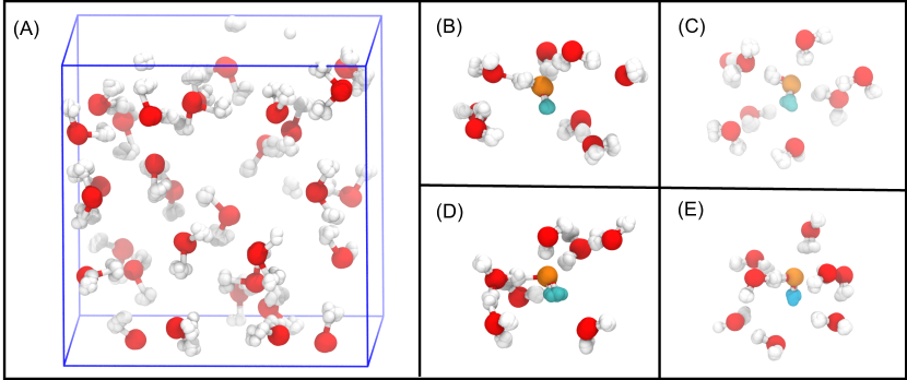
Figure 1:

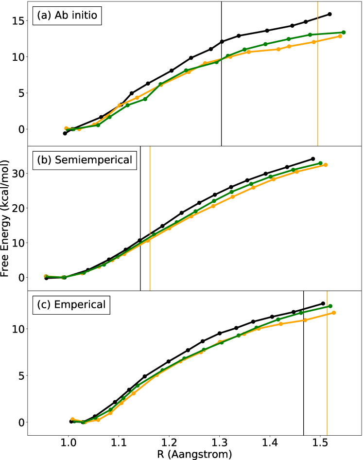
Figure 2:

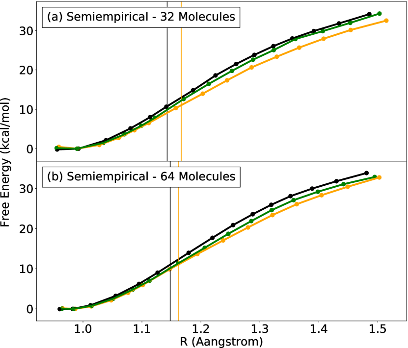
Figure 3:

Table I. Simulation setup of water isotopologues.
Method	System	Molecules	$P$	$\Delta t$ [ps]	Length [ps]	Restraints
DFTa	liq. H2O	32	1	0.25	24.0	15
DFTb	liq. H2O	32	12	0.25	25.0	15
DFTb	liq. D2O	32	12	0.25	25.0	15
DFTb	liq. T2O	32	12	0.25	25.0	15
DFTBc	liq. H2O	32	1	0.25	25.0	15
DFTBd	liq. H2O	32	12	0.25	25.0	15
DFTBd	liq. H2O	32	32	0.25	25.0	15
DFTBd	liq. D2O	32	12	0.25	25.0	15
DFTBd	liq. T2O	32	12	0.25	25.0	15
DFTBd	liq. T2O	32	32	0.25	25.0	15
DFTBd	aq. HDO	32	12	0.25	25.0	15
DFTBd	aq. HTO	32	12	0.25	25.0	15
DFTBc	liq. H2O	64	1	0.25	25.0	15
DFTBd	liq. H2O	64	12	0.25	25.0	15
DFTBd	liq. T2O	64	12	0.25	25.0	15
OSS2e	liq. H2O	64	1	0.25	12.5	15
OSS2f	liq. H2O	64	12	0.25	12.5	15
OSS2f	liq. D2O	64	12	0.35	17.5	15
OSS2f	liq. T2O	64	12	0.43	21.5	15
OSS2f	aq. HDO	64	12	0.25	12.5	15
OSS2f	aq. HTO	64	12	0.25	12.5	15
aAb initio MD.
bAb initio PIMD.
cSemiempirical MD.
dSemiempirical PIMD.
eEmpirical MD.
fEmpirical PIMD.

Table II. Autoionization constants of water isotopologues calculated by
the probabilistic method.
Method	System	Molecules	$P$	p$K_{W}$ (PROB)	$R_{c}$ [Å]
DFTa	liq. H2O	32	12	14.0e	1.50$\pm$0.02
DFTa	liq. D2O	32	12	13.5 $\pm$ 1.2	1.50$\pm$0.02
DFTa	liq. T2O	32	12	15.4 $\pm$ 0.9	1.50$\pm$0.02
DFTBb	liq. H2O	32	12	14.0e	1.16$\pm$0.00
DFTBb	liq. D2O	32	12	15.0 $\pm$ 0.3	1.16$\pm$0.00
DFTBb	liq. T2O	32	12	15.0 $\pm$ 0.2	1.16$\pm$0.00
DFTBb	liq. H2O	32	32	14.0e	1.17$\pm$0.00
DFTBb	liq. T2O	32	32	15.9 $\pm$ 0.3	1.17$\pm$0.00
DFTBb	liq. H2O	64	12	14.0e	1.16$\pm$0.00
DFTBb	liq. T2O	64	12	14.4 $\pm$ 0.2	1.16$\pm$0.00
OSS2c	liq. H2O	64	12	14.0e	1.51$\pm$0.01
OSS2c	liq. D2O	64	12	15.3 $\pm$ 0.5	1.51$\pm$0.01
OSS2c	liq. T2O	64	12	15.6 $\pm$ 0.5	1.51$\pm$0.01
Exptld	liq. H2O	14.00
Exptld	liq. D2O	14.86shoesmith_ionization_1976
Exptld	liq. T2O	15.2ceriotti_nuclear_2016
aAb initio PIMD.
bSemiempirical PIMD.
cEmpirical PIMD.
dExperimental values.
eReference value to determine $R_{c}$.

Table III. Autoionization constants of water isotopologues calculated by
the absolute method.
Method	System	Molecules	$P$	p$K_{W}$ (ABS)
DFTa	liq. H2O	32	1	19.7 $\pm$ 0.3
DFTb	liq. H2O	32	12	15.2 $\pm$ 0.9
DFTb	liq. D2O	32	12	14.8 $\pm$ 0.7
DFTb	liq. T2O	32	12	16.0 $\pm$ 0.8
OSS2c	liq. H2O	64	1	15.0 $\pm$ 0.5
OSS2d	liq. H2O	64	12	13.5 $\pm$ 0.5
OSS2d	liq. D2O	64	12	14.9 $\pm$ 0.7
OSS2d	liq. T2O	64	12	14.6 $\pm$ 0.6
aAb initio MD.
bAb initio PIMD.
cEmpirical MD.
dEmpirical PIMD.

Table IV. Acidity constants of water isotopologues, calculated using Equation (23).
Method	System	p$K_{A}$ (PROP)	$R_{c}$ [Å]
DFTBa	aq. HDO	16.1 $\pm$ 0.1	1.16$\pm$0.00
DFTBa	aq. HTO	16.3 $\pm$ 0.1	1.16$\pm$0.00
OSS2b	aq. HDO	15.6 $\pm$ 0.3	1.51$\pm$0.01
OSS2b	aq. HTO	17.1 $\pm$ 0.4	1.51$\pm$0.01
aSemiempirical PIMD of 32 water molecules with $P=12$.
bEmpirical PIMD of 64 water molecules with $P=12$.

References

- (1) K. S. Alongi and G. C. Shields, “Chapter 8 - Theoretical Calculations of Acid Dissociation Constants: A Review Article,” in Annual Reports in Computational Chemistry (R. A. Wheeler, ed.), vol. 6, pp. 113–138, Elsevier, Jan. 2010.
- (2) E. Alexov, E. L. Mehler, N. Baker, A. M. Baptista, Y. Huang, F. Milletti, J. E. Nielsen, D. Farrell, T. Carstensen, M. H. M. Olsson, J. K. Shen, J. Warwicker, S. Williams, and J. M. Word, “Progress in the prediction of pKa values in proteins,” Proteins, vol. 79, pp. 3260–3275, Dec. 2011.
- (3) J. Ho and M. Coote, “A universal approach for continuum solvent pK a calculations: are we there yet?,” Theor. Chem. Acc., 2010.
- (4) J. Tomasi, B. Mennucci, and R. Cammi, “Quantum Mechanical Continuum Solvation Models,” Chem. Rev., vol. 105, pp. 2999–3094, Aug. 2005.
- (5) S. Miertuš, E. Scrocco, and J. Tomasi, “Electrostatic interaction of a solute with a continuum. A direct utilizaion of AB initio molecular potentials for the prevision of solvent effects,” Chem. Phys., vol. 55, pp. 117–129, Feb. 1981.
- (6) J. B. Foresman, T. A. Keith, K. B. Wiberg, J. Snoonian, and M. J. Frisch, “Solvent Effects. 5. Influence of Cavity Shape, Truncation of Electrostatics, and Electron Correlation on ab Initio Reaction Field Calculations,” J. Phys. Chem., vol. 100, pp. 16098–16104, Jan. 1996.
- (7) J. L. Pascual‐ahuir, E. Silla, and I. Tuñon, “GEPOL: An improved description of molecular surfaces. III. A new algorithm for the computation of a solvent-excluding surface,” J. Comput. Chem., vol. 15, no. 10, pp. 1127–1138, 1994.
- (8) S. Miertuš and J. Tomasi, “Approximate evaluations of the electrostatic free energy and internal energy changes in solution processes,” Chem. Phys., vol. 65, pp. 239–245, Mar. 1982.
- (9) M. Cossi, N. Rega, G. Scalmani, and V. Barone, “Energies, structures, and electronic properties of molecules in solution with the C-PCM solvation model,” J. Comput. Chem., vol. 24, no. 6, pp. 669–681, 2003.
- (10) A. Klamt and G. Schüürmann, “COSMO: a new approach to dielectric screening in solvents with explicit expressions for the screening energy and its gradient,” J. Chem. Soc., Perkin Trans. 2, pp. 799–805, Jan. 1993.
- (11) A. Klamt, “Conductor-like Screening Model for Real Solvents: A New Approach to the Quantitative Calculation of Solvation Phenomena,” J. Phys. Chem., vol. 99, pp. 2224–2235, Feb. 1995.
- (12) A. V. Marenich, C. J. Cramer, and D. G. Truhlar, “Universal Solvation Model Based on Solute Electron Density and on a Continuum Model of the Solvent Defined by the Bulk Dielectric Constant and Atomic Surface Tensions,” J. Phys. Chem. B, vol. 113, pp. 6378–6396, May 2009.
- (13) I. Soteras, C. Curutchet, A. Bidon-Chanal, M. Orozco, and F. J. Luque, “Extension of the MST model to the IEF formalism: HF and B3lyp parametrizations,” J. Mol. Struct. (Theochem), vol. 727, pp. 29–40, Aug. 2005.
- (14) N. L. Doltsinis and M. Sprik, “Theoretical pKa estimates for solvated P(OH)5 from coordination constrained Car–Parrinello molecular dynamics,” Phys. Chem. Chem. Phys., vol. 5, pp. 2612–2618, June 2003.
- (15) M. Schilling and S. Luber, “Determination of pKa Values via ab initio Molecular Dynamics and its Application to Transition Metal-Based Water Oxidation Catalysts,” Inorganics, vol. 7, p. 73, June 2019.
- (16) Y.-L. Chen, N. L. Doltsinis, R. C. Hider, and D. J. Barlow, “Prediction of Absolute Hydroxyl pKa Values for 3-Hydroxypyridin-4-ones,” J. Phys. Chem. Lett., vol. 3, pp. 2980–2985, Oct. 2012.
- (17) J. E. Davies, N. L. Doltsinis, A. J. Kirby, C. D. Roussev, and M. Sprik, “Estimating pKa Values for Pentaoxyphosphoranes,” J. Am. Chem. Soc., vol. 124, pp. 6594–6599, June 2002.
- (18) N. Sandmann, J. Bachmann, A. Hepp, N. L. Doltsinis, and J. Müller, “Copper(II)-mediated base pairing involving the artificial nucleobase 3h-imidazo[4,5-f]quinolin-5-ol,” Dalton Trans., vol. 48, pp. 10505–10515, July 2019.
- (19) A. K. Tummanapelli and S. Vasudevan, “Dissociation Constants of Weak Acids from ab Initio Molecular Dynamics Using Metadynamics: Influence of the Inductive Effect and Hydrogen Bonding on pKa Values,” J. Phys. Chem. B, vol. 118, pp. 13651–13657, Nov. 2014.
- (20) A. K. Tummanapelli and S. Vasudevan, “Ab Initio MD Simulations of the Brønsted Acidity of Glutathione in Aqueous Solutions: Predicting pKa Shifts of the Cysteine Residue,” J. Phys. Chem. B, vol. 119, pp. 15353–15358, Dec. 2015.
- (21) A. K. Tummanapelli and S. Vasudevan, “Ab Initio Molecular Dynamics Simulations of Amino Acids in Aqueous Solutions: Estimating pKa Values from Metadynamics Sampling,” J. Phys. Chem. B, vol. 119, pp. 12249–12255, Sept. 2015.
- (22) C. D. Daub and L. Halonen, “Ab Initio Molecular Dynamics Simulations of the Influence of Lithium Bromide Salt on the Deprotonation of Formic Acid in Aqueous Solution,” J. Phys. Chem. B, vol. 123, pp. 6823–6829, Aug. 2019.
- (23) L. Xu and M. L. Coote, “Methods To Improve the Calculations of Solvation Model Density Solvation Free Energies and Associated Aqueous pKa Values: Comparison between Choosing an Optimal Theoretical Level, Solute Cavity Scaling, and Using Explicit Solvent Molecules,” J. Phys. Chem. A, vol. 123, pp. 7430–7438, Aug. 2019.
- (24) C. C. R. Sutton, G. V. Franks, and G. da Silva, “First Principles pKa Calculations on Carboxylic Acids Using the SMD Solvation Model: Effect of Thermodynamic Cycle, Model Chemistry, and Explicit Solvent Molecules,” J. Phys. Chem. B, vol. 116, pp. 11999–12006, Oct. 2012.
- (25) S. Zhang, “A reliable and efficient first principles-based method for predicting pKa values. III. Adding explicit water molecules: Can the theoretical slope be reproduced and pKa values predicted more accurately?,” J. Comput. Chem., vol. 33, no. 5, pp. 517–526, 2012.
- (26) B. Thapa and H. B. Schlegel, “Calculations of pKa’s and Redox Potentials of Nucleobases with Explicit Waters and Polarizable Continuum Solvation,” J. Phys. Chem. A, vol. 119, pp. 5134–5144, May 2015.
- (27) B. Thapa and H. B. Schlegel, “Density Functional Theory Calculation of pKa’s of Thiols in Aqueous Solution Using Explicit Water Molecules and the Polarizable Continuum Model,” J. Phys. Chem. A, vol. 120, pp. 5726–5735, July 2016.
- (28) N. L. Haworth, Q. Wang, and M. L. Coote, “Modeling Flexible Molecules in Solution: A pKa Case Study,” J. Phys. Chem. A, vol. 121, pp. 5217–5225, July 2017.
- (29) E. A. Carter, G. Ciccotti, J. T. Hynes, and R. Kapral, “Constrained reaction coordinate dynamics for the simulation of rare events,” Chem. Phys. Lett., vol. 156, pp. 472–477, Apr. 1989.
- (30) M. Sprik and G. Ciccotti, “Free energy from constrained molecular dynamics,” J. Chem. Phys., vol. 109, pp. 7737–7744, Nov. 1998.
- (31) A. V. Bandura and S. N. Lvov, “The Ionization Constant of Water over Wide Ranges of Temperature and Density,” J. Phys. Chem. Ref. Data, vol. 35, pp. 15–30, Dec. 2005.
- (32) N. Mora-Diez, Y. Egorova, H. Plommer, and P. R. Tremaine, “Theoretical study of deuterium isotope effects on acid–base equilibria under ambient and hydrothermal conditions,” RSC Adv., vol. 5, pp. 9097–9109, Jan. 2015.
- (33) D. W. Shoesmith and W. Lee, “The ionization constant of heavy water (D2o) in the temperature range 298 to 523 K,” Can. J. Chem., vol. 54, pp. 3553–3558, Nov. 1976.
- (34) M. Sprik, “Computation of the pK of liquid water using coordination constraints,” Chemical Physics, vol. 258, pp. 139–150, Aug. 2000.
- (35) E. Perlt, M. v. Domaros, B. Kirchner, R. Ludwig, and F. Weinhold, “Predicting the Ionic Product of Water,” Sci Rep, vol. 7, pp. 1–10, Aug. 2017.
- (36) M. Štrajbl, G. Hong, and A. Warshel, “Ab Initio QM/MM Simulation with Proper Sampling: “First Principle” Calculations of the Free Energy of the Autodissociation of Water in Aqueous Solution,” J. Phys. Chem. B, vol. 106, pp. 13333–13343, Dec. 2002.
- (37) R. Wang, V. Carnevale, M. L. Klein, and E. Borguet, “First-Principles Calculation of Water pKa Using the Newly Developed SCAN Functional,” J. Phys. Chem. Lett., vol. 11, pp. 54–59, Jan. 2020.
- (38) M. Moqadam, A. Lervik, E. Riccardi, V. Venkatraman, B. K. Alsberg, and T. S. v. Erp, “Local initiation conditions for water autoionization,” PNAS, vol. 115, pp. E4569–E4576, May 2018.
- (39) P. L. Geissler, C. Dellago, D. Chandler, J. Hutter, and M. Parrinello, “Autoionization in Liquid Water,” Science, vol. 291, pp. 2121–2124, Mar. 2001.
- (40) B. L. Trout and M. Parrinello, “Analysis of the Dissociation of H2o in Water Using First-Principles Molecular Dynamics,” J. Phys. Chem. B, vol. 103, pp. 7340–7345, Aug. 1999.
- (41) M. Shiga, “Path Integral Simulations,” in Reference Module in Chemistry, Molecular Sciences and Chemical Engineering, Elsevier, Jan. 2018.
- (42) M. Parrinello and A. Rahman, “Study of an F center in molten KCl,” J. Chem. Phys., vol. 80, pp. 860–867, Jan. 1984.
- (43) R. W. Hall and B. J. Berne, “Nonergodicity in path integral molecular dynamics,” J. Chem. Phys., vol. 81, pp. 3641–3643, Oct. 1984.
- (44) M. Ceriotti, M. Parrinello, T. E. Markland, and D. E. Manolopoulos, “Efficient stochastic thermostatting of path integral molecular dynamics,” J. Chem. Phys., vol. 133, p. 124104, Sept. 2010.
- (45) M. E. Tuckerman, B. J. Berne, G. J. Martyna, and M. L. Klein, “Efficient molecular dynamics and hybrid Monte Carlo algorithms for path integrals,” J. Chem. Phys., vol. 99, pp. 2796–2808, Aug. 1993.
- (46) M. Ceriotti, W. Fang, P. G. Kusalik, R. H. McKenzie, A. Michaelides, M. A. Morales, and T. E. Markland, “Nuclear Quantum Effects in Water and Aqueous Systems: Experiment, Theory, and Current Challenges,” Chem. Rev., vol. 116, pp. 7529–7550, July 2016.
- (47) D. Marx, M. E. Tuckerman, J. Hutter, and M. Parrinello, “The nature of the hydrated excess proton in water,” Nature, vol. 397, pp. 601–604, Feb. 1999.
- (48) G. Cassone, “Nuclear Quantum Effects Largely Influence Molecular Dissociation and Proton Transfer in Liquid Water under an Electric Field,” J. Phys. Chem. Lett., vol. 11, pp. 8983–8988, Nov. 2020.
- (49) D. Chandler, Introduction to Modern Statistical Mechanics. Oxford: Oxford University Press, 1987.
- (50) M. Shiga, “PIMD,” 2020.
- (51) S. Nosé, “A unified formulation of the constant temperature molecular dynamics methods,” J. Chem. Phys., vol. 81, pp. 511–519, July 1984.
- (52) W. G. Hoover, “Canonical dynamics: Equilibrium phase-space distributions,” Phys. Rev. A, vol. 31, pp. 1695–1697, Mar. 1985.
- (53) G. J. Martyna, M. L. Klein, and M. Tuckerman, “Nosé–Hoover chains: The canonical ensemble via continuous dynamics,” J. Chem. Phys., vol. 97, pp. 2635–2643, Aug. 1992.
- (54) G. Kresse and J. Hafner, “Ab initio molecular dynamics for liquid metals,” Phys. Rev. B, vol. 47, pp. 558–561, Jan. 1993.
- (55) G. Kresse and J. Hafner, “Ab initio molecular-dynamics simulation of the liquid-metal–amorphous-semiconductor transition in germanium,” Phys. Rev. B, vol. 49, pp. 14251–14269, May 1994.
- (56) G. Kresse and J. Furthmüller, “Efficiency of ab-initio total energy calculations for metals and semiconductors using a plane-wave basis set,” Comput. Mater. Sci., vol. 6, pp. 15–50, July 1996.
- (57) J. P. Perdew, K. Burke, and M. Ernzerhof, “Generalized Gradient Approximation Made Simple,” Phys. Rev. Lett., vol. 77, pp. 3865–3868, Oct. 1996.
- (58) S. Grimme, J. Antony, S. Ehrlich, and H. Krieg, “A consistent and accurate ab initio parametrization of density functional dispersion correction (DFT-D) for the 94 elements H-Pu,” J. Chem. Phys., vol. 132, p. 154104, Apr. 2010.
- (59) B. Hourahine, B. Aradi, V. Blum, F. Bonafé, A. Buccheri, C. Camacho, C. Cevallos, M. Y. Deshaye, T. Dumitrică, A. Dominguez, S. Ehlert, M. Elstner, T. van der Heide, J. Hermann, S. Irle, J. J. Kranz, C. Köhler, T. Kowalczyk, T. Kubař, I. S. Lee, V. Lutsker, R. J. Maurer, S. K. Min, I. Mitchell, C. Negre, T. A. Niehaus, A. M. N. Niklasson, A. J. Page, A. Pecchia, G. Penazzi, M. P. Persson, J. Řezáč, C. G. Sánchez, M. Sternberg, M. Stöhr, F. Stuckenberg, A. Tkatchenko, V. W.-z. Yu, and T. Frauenheim, “DFTB+, a software package for efficient approximate density functional theory based atomistic simulations,” J. Chem. Phys., vol. 152, p. 124101, Mar. 2020.
- (60) M. Elstner, D. Porezag, G. Jungnickel, J. Elsner, M. Haugk, T. Frauenheim, S. Suhai, and G. Seifert, “Self-consistent-charge density-functional tight-binding method for simulations of complex materials properties,” Phys. Rev. B, vol. 58, pp. 7260–7268, Sept. 1998.
- (61) M. Gaus, A. Goez, and M. Elstner, “Parametrization and Benchmark of DFTB3 for Organic Molecules,” J. Chem. Theory Comput., vol. 9, pp. 338–354, Jan. 2013.
- (62) L. Ojamäe, I. Shavitt, and S. J. Singer, “Potential models for simulations of the solvated proton in water,” J. Chem. Phys., vol. 109, pp. 5547–5564, Sept. 1998.
- (63) J. Sala, E. Guàrdia, and M. Masia, “The polarizable point dipoles method with electrostatic damping: Implementation on a model system,” J. Chem. Phys., vol. 133, p. 234101, Dec. 2010.
- (64) N. Michaud-Agrawal, E. J. Denning, T. B. Woolf, and O. Beckstein, “MDAnalysis: A toolkit for the analysis of molecular dynamics simulations,” J. Comput. Chem., vol. 32, no. 10, pp. 2319–2327, 2011.
- (65) R. J. Gowers, M. Linke, J. Barnoud, T. J. E. Reddy, M. N. Melo, S. L. Seyler, J. Domański, D. L. Dotson, S. Buchoux, I. M. Kenney, and O. Beckstein, “MDAnalysis: A Python Package for the Rapid Analysis of Molecular Dynamics Simulations,” Proceedings of the 15th Python in Science Conference, pp. 98–105, 2016.
- (66) H. Flyvbjerg and H. G. Petersen, “Error estimates on averages of correlated data,” J. Chem. Phys., vol. 91, pp. 461–466, July 1989.
- (67) W. Humphrey, A. Dalke, and K. Schulten, “VMD: Visual molecular dynamics,” J. Mol. Graph., vol. 14, pp. 33–38, Feb. 1996.
- (68) M. Shiga and H. Fujisaki, “A quantum generalization of intrinsic reaction coordinate using path integral centroid coordinates,” J. Chem. Phys., vol. 136, p. 184103, May 2012.
- (69) M. Machida, K. Kato, and M. Shiga, “Nuclear quantum effects of light and heavy water studied by all-electron first principles path integral simulations,” J. Chem. Phys., vol. 148, p. 102324, Dec. 2017.
- (70) T. P. Silverstein and S. T. Heller, “pKa Values in the Undergraduate Curriculum: What Is the Real pKa of Water?,” J. Chem. Educ., vol. 94, pp. 690–695, June 2017.
- (71) E. C. Meister, M. Willeke, W. Angst, A. Togni, and P. Walde, “Confusing Quantitative Descriptions of Brønsted-Lowry Acid-Base Equilibria in Chemistry Textbooks – A Critical Review and Clarifications for Chemical Educators,” Helv. Chim. Acta, vol. 97, no. 1, pp. 1–31, 2014.