One-parameter robust global frequency estimator for slowly varying amplitude and noisy oscillations

Abstract

Robust online estimation of oscillation frequency belongs to classical problems of system identification and adaptive control. The given harmonic signal can be noisy and with varying amplitude at the same time, as in the case of damped vibrations. A novel robust frequency-estimation algorithm is proposed here, motivated by the existing globally convergent frequency estimator. The advantage of the proposed estimator is in requiring one design parameter only and being robust against measurement noise and initial conditions. The proven global convergence also allows for slowly varying amplitudes, which is useful for applications with damped oscillations or additionally shaped harmonic signals. The proposed analysis is simple and relies on an averaging theory of the periodic signals. Our results show an exponential convergence rate, which depends, analytically, on the sought frequency, adaptation gain and oscillation amplitude. Numerical and experimental examples demonstrate the robustness and efficiency of the proposed estimator for signals with slowly varying amplitude and noise.

1 Introductory note

A common problem associated with online estimation of the unknown frequency of harmonic signals has been studied in multiple works (see, e.g., [1, 2, 3, 4, 5] and references in the latter). Some differing approaches rely on extended observer or Kalman filter principles (see, e.g., [6]). Other approaches (particularly those accommodated in power electronics applications) use so-called phase-locked-loop (PLL) algorithms (see, e.g., [7]). Frequency estimation can be seen to be one of the fundamental questions in systems and signals theory, and it has multiple practical mechanical and electrical applications. For instance, it can be found in the following: power system converters and controllers (e.g., [7]); active control of sound and vibrations (e.g., [8]); rotary machines, like in magnetic bearings (e.g., [9]); drives with eccentricities (e.g., [10]); and motion control with periodic and vibrational disturbances of, e.g., disk drives [11] or suspensions [12], to mention just a few.

In several application scenarios, like in the case of damped vibrations, the time-varying amplitude of a harmonic signal is, however, the most challenging factor for robust and sufficiently fast estimation of the unknown frequency. Besides, measurement and process noise can further degrade those estimation approaches for which the convergence is theoretically proven, but which can suffer through sensitivity to real measured (physical) data, making their applicability questionable in terms of robust convergence. Among the numerous existing frequency-estimation methods, the globally convergent estimator, introduced in [2], appears promising due to its structural simplicity and low number of design parameters. This paper focuses on the globally convergent frequency estimator (cf. [2, 4]) and proposes a one-parameter robust modification, which targets unbiased harmonic signals with a slowly varying amplitude and band-limited white noise.

The rest of the paper is structured as follows. The problem statement for a noisy harmonic signal with slowly varying amplitude and an unknown frequency of interest is given in Section 2. The existing globally convergent frequency estimator (relevant to this work) is summarized in Section 3. In this regard, differences in the proposed estimator (and therefore the contributions of the paper) are highlighted. The main results, with corresponding analysis and proofs, are provided in Section 4. In Section 5, various simulated and experimental harmonic signals are shown as confirming the highlighted estimator properties. Brief conclusions are drawn in Section 6.

2 Problem statement

We consider a classical estimation problem, which is of importance for system identification and adaptive control, where a signal of the form

$$\sigma(t)=k(t)\sin(\omega_{0}t)+\eta(t),$$ (1)

is the single measured oscillating quantity. The harmonic signal has a slowly varying amplitude within a certain range $\underline{k}\leq k\leq\overline{k}$, and an unknown angular frequency $\omega_{0}>0$, which we are mainly interested in. The measured $\sigma(t)$ is affected by the noise $\eta(t)$, which is a zero-mean ergodic process uniformly distributed over the whole frequency range $\omega$. In other words, $\eta(t)$ can be seen as power-limited (and therefore band-limited) white noise, seen from a signal-processing viewpoint. We will assume a constant power spectral density (PSD) of the noise, i.e., $\mathrm{PSD}\{\eta(\omega)\}\equiv p=\mathrm{const}$, and a reasonable (in terms of the signal-to-noise ratio) finite variance $\mathrm{Var}\{\eta(t)\}=\tau^{2}$, this without going into further details about the spectral properties of $\eta(j\omega)$.

Although biased sinusoids with unknown frequency are often considered (e.g., [3, 13]), this work focuses only on unbiased sinusoidal signals (1), while keeping in mind that some constant bias can be removed by high-pass or other dedicated filtering approaches. Rather, we emphasize that $k(t)$ can be slowly varying. For instance, if one allows for $k(t)\rightarrow 0$ with the progressing time, then (1) will represent a damped oscillation response $\sigma(t)$, where only a finite number of the periods is available for estimating $\omega_{0}$.

3 Globally convergent adaptive notch filter

The globally convergent adaptive filter (also denoted as an adaptive notch filter (ANF) due to the structural properties of a second-order notch filter) was provided and analyzed in [2], based on the original work [14]. A continuous-time version of the ANF [14] can also be found in [1]. The ANF considers a sinusoidal signal (1) but without explicit amplitude variation $k(t)$ and noise $\eta(t)$, and estimates the unknown frequency $\omega_{0}$ using the following structure [2]:

$$\ddot{x}+2\zeta\theta\dot{x}+\theta^{2}x = \theta^{2}\sigma,$$ (2)

$$\dot{\theta} = -\gamma x\bigl{(}\theta^{2}\sigma-2\zeta\theta\dot{x}\bigr{)}.$$ (3)

Subsequently, another scaling of the forcing signal in (2) and, correspondingly, error signal in (3) was proposed and analyzed in [4], while it was claimed that the adaptation scheme and necessary stability condition become independent of the damping ratio $\zeta$. Both aforementioned formulations of the ANF have two real positive design parameters: $\gamma$, which determines the ’adaptation speed’, and $\zeta$, which determines the ’depth of the notch’ and hence noise sensitivity, according to [4]. In both approaches [2, 4], stability analysis and proof of convergence rely on the concept of the uniqueness of a periodic orbit $\bigl{[}\bar{x},\bar{\dot{x}},\bar{\theta}\bigr{]}(t)$, where $(\bar{\cdot})$ denotes equilibria (not necessarily constant). Towards this unique orbit, with $\bar{\theta}=\omega_{0}$, the adaptive system (2), (3) is then shown to converge globally. Since its appearance, the ANF approach has become popular, and performance, design equations and applications, as well as signal/noise ratios and initialization, have been addressed in several works (see, e.g., [15]).

The estimator introduced below keeps the same motivating ANF principle while (i) adapting the scaling factor, (ii) using the sign instead of the $x$-state in (3), and (iii) canceling the damping ratio design parameter, which is shown to be unnecessary. The proposed convergence analysis is based on a simpler consideration of steady states in the frequency domain, through keeping $\theta$ as a frozen parameter, which avoids the challenges of demonstrating convergence of (2), (3) into a unique periodic orbit (cf. [2, 4]). At the same time, we can demonstrate explicitly an exponential convergence rate and can take into account (explicitly) the impact of measurement noise and (implicitly) insensitivity to slow amplitude variations.

4 Main results

The proposed robust global frequency estimator is provided by the auxiliary second-order system

$$\left[\begin{array}[]{c}\dot{x}_{1}\\ \dot{x}_{2}\\ \end{array}\right] = \left[\begin{array}[]{cc}0&1\\ -\theta^{2}&-2\theta\\ \end{array}\right]\left[\begin{array}[]{c}x_{1}\\ x_{2}\\ \end{array}\right]+\left[\begin{array}[]{c}0\\ 2\theta\\ \end{array}\right]\sigma,$$ (12)

$$y = \left[\begin{array}[]{cc}0&1\\ \end{array}\right]\left[\begin{array}[]{c}x_{1}\\ x_{2}\\ \end{array}\right],$$ (16)

and the adaptation law

$$\dot{\theta}=-\gamma\,\mathrm{sign}(x_{1})(\sigma-y),$$ (17)

where $\gamma>0$ appears as the single design parameter. Being excited by $\sigma(t)$, the vector of dynamic states $[x_{1},x_{2}]^{T}$ performs steady-state oscillations at the angular frequency $\theta=\omega_{0}$, once the input-output synchronization brings the output error to zero, i.e., $e=\sigma-y\rightarrow 0$. For a slowly varying $k(t)$, the $2\theta$ input coupling factor used (on the right-hand side of (12)) endows the input-output ratio of (12), (16) to be independent of $k$ in a steady state, thus making a frequency estimation insensitive to slow amplitude variations. It is also worth noting that, unlike similar adaptation mechanisms [2], [4], no further scaling factors are assigned to the forcing signal $\sigma(t)$. A clear advantage of this purposeful simplification will be shown later when analyzing the convergence rate. While an ANF contains an additional damping parameter, which determines the ’depth of the notch’ and, according to [2, 4], its noise sensitivity, we deliberately assume a critically damped dynamic system (12), (16) (compared with (2) for $\zeta=1$). This simplification not only removes the second design parameter but also eliminates transient oscillations of $\theta(t)$ in the course of the frequency adaptation. This comes as no surprise since the linear $[x_{1},x_{2}]^{T}$ sub-dynamics with $\zeta=1$ have no conjugate-complex poles and therefore no transient oscillations (thus also not in $e(t)$). Later, we will demonstrate a performance degradation when a damping factor $0<\zeta<1$ is included, as a parameter, in (12), (16).

Denoting the system matrix and input and output coupling vectors in (12), (16) by $A$, $B$ and $C$, correspondingly, the input-to-output transfer function

$$G(j\omega)=\frac{y(j\omega)}{\sigma(j\omega)}=C^{T}(j\omega I-A)^{-1}B,$$ (18)

can be written for the frequency domain, when $\theta$ is considered to be a frozen parameter. Obviously, $I$ is the $2\times 2$ identity matrix, and $\omega$ is the angular frequency variable. As long as the output error is not zero, it is excited as

$$e(j\omega)=(1-G)G^{-1}y(j\omega),$$ (19)

by the forced dynamics (12), (16), so that $\bigl{|}e(j\omega)\bigr{|}>0$ for all $\omega$ excepts $\omega=\omega_{0}$. This motivates the adaptation law (17), which ensures $\dot{\theta}\neq 0$ always excepts at $\theta=\omega_{0}$. Denoting the above transfer function, i.e., from the filter output to the error, by

$$E(j\omega)=\frac{e(j\omega)}{y(j\omega)}=\bigl{(}1-G(j\omega)\bigr{)}G(j\omega)^{-1},$$

we can take a closer look at the amplitude and phase response of $E(\cdot)$, illustrated in Fig. 1 for $\theta=10$ rad/sec.

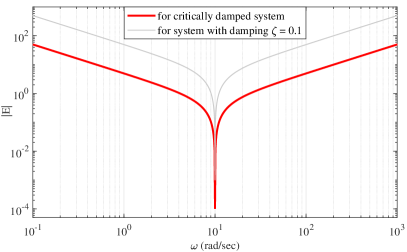
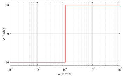
Figure 1: Amplitude and phase response of the transfer function $E$, for exemplary $\theta=10$ rad/sec; the transfer function with an additional damping $\zeta=0.1$ (cf. with (1)) is included (gray line) for the sake of comparison.

It becomes evident that the error transfer function amplitude $|E|$ has global minima at $\omega=\theta$, so that $|e(j\omega)|\rightarrow 0$ when $\theta(t)\rightarrow\omega_{0}$, and this is independent of the estimator initialization $\theta(0)$. Indeed, without loss of generality, we can assume an arbitrary $0<\theta(0)\neq\omega_{0}$ so that $\bigl{|}e(j\omega)\bigr{|}_{\omega=\omega_{0}}=a$, where $a>0$ is some positive magnitude determined by the oscillating output state and error transfer function. We also recall that the oscillating output in a steady state will then be given by $y=G(j\omega)\sigma$, since the system (12), (16) is asymptotically stable and, moreover, critically damped. This basically leads to the harmonic behavior of $y(t)$ and $e(t)$, provided $\omega_{0}=\mathrm{const}.$

Further, it becomes evident (cf. phase response in Fig. 1) that $\angle e(j\omega)$ always lags behind the phase $\angle y(j\omega)$ for $\omega<\omega_{0}$, which is due to $\angle E(j\omega)\rightarrow-\pi/2$. Correspondingly, $\angle e(j\omega)$ always leads before the phase $\angle y(j\omega)$ for $\omega>\omega_{0}$, which is due to $\angle E(j\omega)\rightarrow\pi/2$. It is only at $\omega=\omega_{0}$ where both signals $y(j\omega)$ and $e(j\omega)$ are in the phase and $e\rightarrow 0$. The $\pm\pi/2$ phase response of $\angle E(j\omega)$ allows for providing an ever-increasing or decreasing $\theta(t)$ on the left-hand or, respectively, right-hand side of $\omega_{0}$. With this in mind, we are now in a position to formally prove global convergence of the adaptation law (17).

Theorem 1.

The frequency estimator (12)-(17) is global for (1) and converges asymptotically as $\theta(t)\rightarrow\omega_{0}$ for $t\rightarrow\infty$, regardless of the $\theta(0)>0$ initialization, provided the small adaptation gains $\gamma>0$ and slowly varying amplitudes $k(t)$. The frequency-estimation error $\varepsilon(t)=\omega_{0}-\theta(t)$ converges uniformly and exponentially in terms of

$$\bigl{|}\varepsilon(t_{2})\bigr{|}<\alpha\bigl{|}\varepsilon(t_{1})\bigr{|}\exp\bigl{(}-\beta(t_{2}-t_{1})\bigr{)}$$ (20)

for some $\alpha>0$ and $\forall\;t_{2}>t_{1}$. The exponential rate of convergence is independent of $\eta(t)$ noise, as follows:

$$\beta=0.5\,\gamma k\,\omega_{0}^{-1}+\delta,$$ (21)

where $\delta$ is a small positive constant independent of $\gamma$, $k$, $\omega_{0}$.

Proof.

Let $0<\theta(0)<\omega_{0}$ be an arbitrary initialization of the estimator (12)-(17). Note that for $\theta(0)>\omega_{0}$, the proof is fully identical due to the phase symmetry of $\angle E\bigl{(}j\theta\bigr{)}\rightarrow\pm\pi/2$ for all $\theta\neq\omega_{0}$, and as a consequence, $\mathrm{sign}\bigl{(}\dot{\theta}\bigr{)}=\pm 1$. A harmonic excitation (1) leads to an output harmonic

$$y(t)=b\sin(\omega_{0}t+c),$$ (22)

where $b=k\bigl{|}G(j\omega_{0})\bigr{|}$, while the phase shift $c=\angle\bigl{(}G(j\omega_{0})\bigr{)}$ is of minor relevance here. The internal dynamic state of the estimator then becomes

$$x_{1}(t)=-\frac{b}{\omega_{0}}\cos(\omega_{0}t+c)=-\frac{b}{\omega_{0}}\sin(\omega_{0}t+c+\pi/2),$$ (23)

and the output error becomes

$$e(t)=a\sin(\omega_{0}t+c+\pi/2),$$ (24)

where $a=b|E(j\omega_{0})|>0$ for all $\theta<\omega_{0}$. Substituting (23) and (24) into (17), and writing out $a$ and $b$, results in

$$\dot{\theta}=\gamma k\,\bigl{|}G(j\omega_{0})\bigr{|}\,\Bigl{|}\frac{1-G(j\omega_{0})}{G(j\omega_{0})}\Bigr{|}\,\bigl{|}\sin(\omega_{0}t+c+\pi/2)\bigr{|}.$$ (25)

It is clear that for all $\gamma,k>0$ the $\mathrm{sign}(\dot{\theta})=+1$ as long as $\theta(t)<\omega_{0}$. This implies global uniform convergence and completes the first part of the proof.

Evaluating the first and second modulus $|\cdot|$-terms in (25)

$$\bigl{|}G(j\omega_{0})\bigr{|}\,\Bigl{|}\frac{1-G(j\omega_{0})}{G(j\omega_{0})}\Bigr{|}=\frac{\bigl{|}\theta^{2}-\omega_{0}^{2}\bigr{|}}{\theta^{2}+\omega_{0}^{2}}\equiv\Omega(\theta),$$ (26)

one can show that the $\theta$-dependent magnitude $\Omega$ always decreases monotonically and $1\geq\Omega(\theta)\geq 0$ on the interval $\theta\in[0,\,\omega_{0}]$. Inspecting the $\Omega(\theta)$ function, with the $\omega_{0}$-normalized argument, as depicted in Fig. 2,

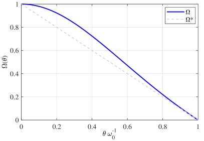
Figure 2: $\Omega(\theta)$ function of the $\omega_{0}$-normalized argument.

one can linearly approximate the magnitude of the decrease by

$$\Omega^{*}(\theta)=-\theta\omega_{0}^{-1}+1.$$ (27)

Using (27) and the fact of an always positive third modulus $|\cdot|$-term in (25), which has a mean value equal to $1/2$, one can write the first-order approximation

$$\dot{\theta}^{*}=0.5\,\gamma k\bigl{(}-\theta^{*}\omega_{0}^{-1}+1\bigr{)}$$ (28)

of the estimator dynamics. Note that the $\angle E\bigl{(}j\theta\bigr{)}\rightarrow\pm\pi/2$ phase, which determines the sign of $\dot{\theta}$ (cf. (25)), allows us to write (28), regardless of whether $\theta^{*}(0)<\omega_{0}$ or $\theta^{*}(0)>\omega_{0}$. Because of (27) is an under-approximation of the $(\theta\omega_{0}^{-1})$-dependent gaining factor of the adaptation rate (cf. Fig. 2), the following can be concluded from the eq. (28). The asymptotic convergence of $\theta(t)$ to $\omega_{0}$ has an exponential rate of $0.5\gamma k\omega_{0}^{-1}+\delta$, which is not slower than that of the dynamics

$$\dot{\theta}(t)+0.5\gamma k\omega_{0}^{-1}\theta(t)=0.5\gamma k\omega_{0}^{-1}\cdot\omega_{0},$$ (29)

(cf. (28) and (29)). This completes the second part of the proof. ∎

Remark 1.

Note that the asymptotic convergence of $\theta(t)$ can be guaranteed firstly when $y(t)$ is in a steady state, i.e., after the transients of (12), (16) dynamics excited by (1). The transient response results in a temporary bias of the output harmonic $y(t)$, depending on the initial phase of the excitation signal $\sigma(t)$. Consequently, the $\theta(t)$ trajectory can drift oscillatory in the opposite direction, away from $\omega_{0}$, until $y(t)$ is in a steady state (cf. the first numerical example in Section 5.1). This initial by-effect must be taken into account when assigning $0<\theta(0)<\omega_{0}$, while being irrelevant for $\theta(0)>\omega_{0}$.

Remark 2.

When including the damping factor $0<\zeta<1$ as an additional design parameter of the estimator (cf. [2, 4]), the dynamic system (12), (16) needs to be modified in respect of the $A$ and $B$ terms (cf. with (2)) and consequently becomes non-critically damped. By implication, additional oscillating dynamics of $y(t)$ appear, both during the transients and with a steady state of the dynamic $\theta(t)$ trajectory. Notice that $\zeta$ has a minor influence on the asymptotic convergence and its exponential rate (cf. Fig. 1 for $\zeta=0.1$). At the same time, it deteriorates the smoothness of $\theta(t)$ during the transient phase and produces residual steady-state oscillations of $\varepsilon(t)$ (cf. $\theta(t)$-trajectories, exemplified in Fig. 3 for $\zeta=\{0.1,0.5,1\}$).

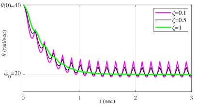
Figure 3: Convergence trajectories of the estimator ($\gamma=100$, $\omega_{0}=20$ rad/sec) with additional damping $\zeta=\{0.1,0.5,1\}$.

Once we have shown the asymptotic convergence of $\theta(t)$ to $\omega_{0}$ and estimated the exponential convergence rate, it is of further interest to analyze the non-vanishing residual $\varepsilon(t)$, depending on the signal noise $\eta(t)$.

Lemma 2.

The residual frequency-estimation error is a zero-mean ergodic process, with

$$\mathrm{Var}\{\varepsilon(t)\}<4\tau^{2}\omega_{0}k^{-1},$$ (30)

for the signal (1) with band-limited white noise, which has variance $\mathrm{Var}\{\eta(t)\}=\tau^{2}$.

Note that the Lemma 2 claims the upper bound of the second moment of $\varepsilon(t)$ for all times $t>t_{c}>0$, since $\varepsilon(t)$ is a random process driven by $\eta(t)$, after $\theta(t)$ has converged to a neighborhood of $\omega_{0}$ at some finite time $t_{c}$.

Proof.

Denoting the harmonic part of the signal (1) by $\tilde{\sigma}(j\omega_{0})$ and that of the output (16) by $\tilde{y}(j\omega_{0})$, respectively, the output error in the frequency domain can be written as

$$e(j\omega)=\tilde{\sigma}(j\omega_{0})-\tilde{y}(j\omega_{0})+\eta(j\omega)-G(j\omega)\eta(j\omega).$$ (31)

Provided the estimator has already converged to a neighborhood of $\omega_{0}$, the harmonic part of the error can be set to zero, and the residual error, due to the noise, is to be analyzed further. Since no phase response can be considered for a stochastic noise signal (only the magnitude), one can assume

$$|\hat{e}(j\omega)|=2|\eta(j\omega)|$$ (32)

as a worst case (i.e., upper bound) since $\|G(j\omega)\|_{\infty}=1$. Using the variance (for the noise magnitude) and substituting it into (17), one can write the noise-driven dynamics of the estimate as

$$|\dot{\hat{\theta}}|=\gamma\,2\tau^{2},$$ (33)

for some neighborhood $\hat{\theta}$ of the true value $\omega_{0}$. Note that the sign of $\dot{\hat{\theta}}$ is also a random process driven by $\mathrm{sign}\bigl{(}x_{1}(t,\eta)\bigr{)}\,\mathrm{sign}\bigl{(}\eta(t)\bigr{)}$ (cf. with (17)). Now, comparing (25) and (33), one can see that for the estimate dynamics not driven by noise, the following inequality should hold

$$\mathrm{sign}\bigl{(}\dot{\theta}\bigr{)}=\mathrm{const}=\gamma\,0.5k\,\Omega(\theta)>\gamma\,2\tau^{2}.$$ (34)

Using the linear approximation (27), and substituting it into (34), yields

$$k\Bigl{(}-\frac{\theta}{\omega_{0}}+1\Bigr{)}>4\tau^{2}.$$ (35)

Solving (35) with respect to $|\varepsilon|=|\omega_{0}-\theta(t)|$ results in

$$|\varepsilon|>4\tau^{2}\omega_{0}k^{-1},$$ (36)

which should be fulfilled so that the estimate dynamics (17) do not become driven by the signal noise. Turning back to the random nature of the noise-driven residual estimation error, one can state (30) (cf. with (36)), which completes the proof. ∎

5 Numerical and experimental examples

5.1 Simulated signals

We firstly demonstrate convergence of the estimator (12)-(17) for a purely sinusoidal signal $\sigma(t)=\sin(\omega_{0}t)$, i.e., with a constant unity amplitude and without noise. Assuming two estimator initializations $\theta(0)=\{10,100\}$ rad/sec, i.e., one higher and one lower than $\omega_{0}=50$ rad/sec, the $\theta(t)$ trajectories are shown in Fig. 4 for $\gamma=\{200,100,50\}$ adaptation gains.

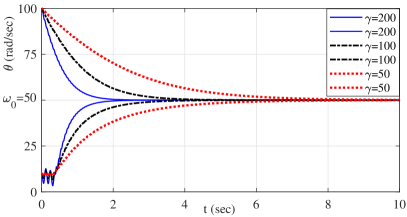
Figure 4: Convergence of $\theta(t)$ with $\gamma=\{200,100,50\}$ to $\omega_{0}=50$ rad/sec for $\sigma(t)=\sin(\omega_{0}t)$ signal with constant amplitude and without noise.

The resulting exponential shape of convergence is in accord with (21). Note that for $\theta(0)=10$ rad/sec, the initial $\theta(t)$ trajectory is oscillatory, progressing in the opposite direction. This occurs due to a transient response of (12), (16) to the $\sigma$-excitation, which takes about three oscillation periods for the given $\theta(0)$ and $\omega_{0}$ values (cf. Remark 1).

Next, we consider the signal (1) with $k=1$ for different $\omega_{0}=\{10,30,50,70\}$ rad/sec. For all angular frequencies, an additional band-limited white noise $\eta(t)$ with $p=1e-7$ and $\tau^{2}=0.001$ is included, as exemplified in Fig. 5 (a) for $\omega_{0}=10$ rad/sec. The adaptation gain is set to $\gamma=100$.

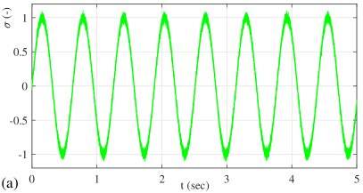
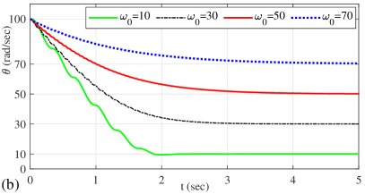
Figure 5: (a) Simulated signal (1) with $k=1$, $\omega_{0}=10$ rad/sec; (b) convergence of $\theta(t)$ with $\gamma=100$ for $\omega_{0}=\{10,30,50,70\}$ rad/sec.

The convergence of $\theta(t)$ depends inversely on $\omega_{0}$ and is in accord with (21), as can be seen from Fig. 5 (b). Note that the noise of $\eta(t)$ does not affect the convergence rate but solely the steady-state fluctuations of the residual estimation error $\varepsilon(t)$, in accord with the Lemma 2.

To demonstrate insensitivity of the frequency estimator to the slow amplitude variations of the signal (1), we consider $\omega_{0}=40$ rad/sec with $k(t)=5+5\sin(0.9t-\pi/2)$, as depicted in Fig. 6 (a).

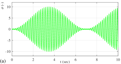
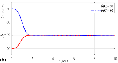
Figure 6: (a) Simulated signal (1) with $k(t)=5+5\sin(0.9t-\pi/2)$ and $\omega_{0}=40$ rad/sec; (b) convergence of $\theta(t)$ with $\gamma=100$.

For the adaptation gain $\gamma=100$ and two different estimator initializations $\theta(0)=\{20,80\}$, the $\theta(t)$ convergence is shown in Fig. 6 (b). After a stable transient of $\theta(t)$, whose shape is dynamically affected by the $k(t)$ variations, the estimation error $\varepsilon(t)$ in a steady state (for $t>1.8$ sec) does not appear to be affected by persistent variations in the amplitude $k(t)$.

Finally, we are eager to see how the proposed robust estimator can deal with the continuously varying frequencies $\omega_{0}(t)$. For this purpose, the simulated signal (1) with $k=1$ is designed as a linear down-chirp $\omega_{0}(t)=\omega_{0}(0)-\mu t$, with the frequency bounds $\omega_{0}(0)=20\cdot 2\pi$ rad/sec and $\omega_{0}(30)=1\cdot 2\pi$ rad/sec, and the resulting $\mu=3.98$, as depicted in Fig. 7 (a).

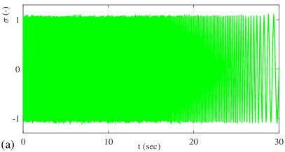
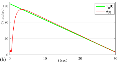
Figure 7: (a) Simulated signal (1) with $k=1$, $\omega_{0}(t)=\omega_{0}(0)-\mu t$; (b) convergence of $\theta(t)$ with $\gamma=200$, $\theta(0)=10$ rad/sec.

The $\theta(t)$ trajectory, for the assigned $\gamma=200$, is shown in Fig. 7 (b) versus the linearly changing $\omega_{0}(t)$. It can be seen that after a certain time, the $\theta(t)$ trajectory closely follows $\omega_{0}(t)$. The visible residual estimation error $\varepsilon(t)\neq 0$ is clearly due to the dynamically changing excitation frequency $\omega_{0}$; a more detailed analysis of this effect is beyond the scope of this work. Still, the estimator appears sufficiently robust to also follow a continuously varying excitation frequency.

5.2 Experimental case

The proposed frequency estimation algorithm can equally be used for mechanical system applications in which the oscillating behavior (including vibrations) of structural parts and elements with elasticities requires tracking of the frequency for various purposes. Those include, e.g., controller tuning, condition and fault monitoring, commissioning and identification, and others. An experimental case provided below is realized in a laboratory setting which is still representing a standard situation of an unknown mechanical oscillation frequency in combination with a low damping. Such application scenarios are commonly appearing in two-inertia systems with either a load-depending varying natural frequency, like in the flexible robotic joints (see e.g. [16, 17]) and machine tools and instruments with cantilevers and flexible frames (see e.g. [18, 19]). Or it is associated with problems of varying excitation frequencies that propagate through a flexible, correspondingly oscillating structure (see e.g. [20, 21]).

For benchmarking with existing frequency estimators of the same principle (cf. Sections 1, 3), the ANF modified and proposed in [4] was also implemented, in the same numerical setting as the proposed algorithm (12)-(17). Both frequency estimators are then evaluated, as described below, on the same experimental data and for the same initial and parametric conditions.

The case study with a simultaneous variation of the signal amplitude $k(t)$ and angular frequency $\omega_{0}(t)$ is evaluated experimentally suing the laboratory setup [22] shown in Fig. 8. More details on the system dynamics and modeling, that is however of lower relevance for the recent work, an interested reader is referred to [23].

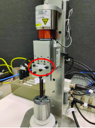
(a)   (b)

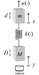
Figure 8: Experimental setup: (a) laboratory view of the two-mass oscillator, passive free-hanging mass ($M$) is placed on the holder-disc when not in operation; (b) schematic representation of two-mass oscillator, oscillating displacement $y\equiv\sigma(t)$ is measured contactlessly.

The oscillating displacement of a free hanging load, attached through a nearly linear spring ($K$), is measured contactlessly by means of an inductive distance sensor, which has $\pm 12$ $\mu$m repeatability. The sampling rate of real-time measurements, analog to digital conversion with 16-bit quantization, is 2 kHz. Being subject to both sensing ($\eta(t)$) and process disturbances (non-modeled $d$ and $D$), the measured response $\sigma(t)$ constitutes an oscillating and noisy (cf. zoom-in in Fig. 9) time series. The double-mass experimental setup, with the first ’active’ mass ($m$) of the voice-coil-motor actuator and second ’passive’ mass ($M$) of a free hanging load, allows for testing of the eigendynamics response and excited (i.e., input-driven) response, both of a low-damped oscillating nature.

The measured signal (Fig. 9) represents an exemplary response to an actuated chirp excitation, which yields a linearly increasing angular frequency $\omega_{0}(t)=\mu t$, with some initial value and $\mu>0$. The measured displacement $\sigma(t)$ is freed (by data postprocessing) from a steady-state offset, thus approaching a single harmonic, in accord with (1). Note that apart from the noise, the measured $\sigma(t)$ is still slightly affected by an asymmetry around zero, therefore disclosing a certain additional non-constant bias.

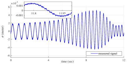
Figure 9: Experimentally measured signal $\sigma(t)$ with varying amplitude $k(t)$ and linearly increasing angular frequency $\omega_{0}(t)$.

The evaluation setting, in terms of the parameters and initial conditions, is summarized in Table 1 for both estimators under benchmark.

Table 1: Estimators’ evaluation setting

Set parameter	ANF according to [4]	Proposed estimator
$\theta(0)$ (rad/sec)	20	20
$\gamma$	$4e4$	$2e4$
$\zeta$	$\{0.7,\,1,\,1.3\}$	$\{0.7,\,1,\,1.3\}$

Note that for the proposed estimator, the assigned $\gamma$-gain is twice smaller than $\gamma$ for the ANF [4], since for the latter it is already integrating the factor $2\zeta$, cf. [4, eqs. (5),(6)]. Further, for the sake of completeness and a fair comparison, the damping ratio $\zeta$ is additionally included into the proposed estimator. Recall that, otherwise, $\zeta=1$ is set as default and is not appearing as a design parameter, according to (12)-(17).

The online estimate of the angular frequency $\theta(t)$ is shown in Fig. 10 versus the linear progress of the chirp-driven true $\omega_{0}(t)$ value. The estimated $\theta(t)$ values are plotted over each other for the ANF [4] and the proposed estimator, for $\zeta=0.7$ in (a), for $\zeta=1$ in (b), and for $\zeta=1.3$ in (c), correspondingly.

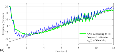
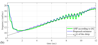
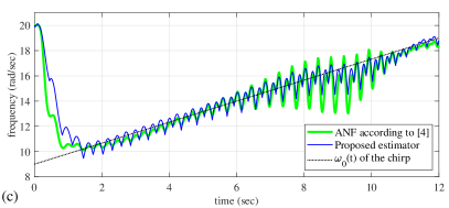
Figure 10: Online estimate of the angular frequency $\theta(t)$ versus the chirp-driven $\omega_{0}(t)$: (a) for $\zeta=0.7$, (b) $\zeta=1$, and (c) for $\zeta=1.3$.

One can recognize that in all three cases, the proposed estimation algorithm follows the varying true angular frequency similarly as [4] at the benefit of one design parameter. The transient convergence appears slightly faster, and less deviations to $\omega_{0}(t)$ appear for the critically damped case of $\zeta=1$.

6 Conclusions

In this paper, the problem of estimating the unknown frequency of noisy sinusoidal signals with slowly varying amplitude has been considered. The existing globally convergent frequency estimator was modified by changing the scaling of the excitation signal and output error, and canceling the damping ratio as a free design parameter. Furthermore, the main robustification was achieved by using the sign of an internal state, instead of the state itself, within the adaptation law. Relying on the averaging theory of periodic signals, an easy-to-follow and straightforward analysis was developed in the frequency domain, assuming that the timescales of a relatively fast harmonic (to be estimated) and relatively slow drift of the amplitude can be separated. We analyzed and proved the global asymptotic convergence of the frequency estimate and determined the exponential convergence rate. The dependency between band-limited white noise and the resulting residual estimation error in a steady state was established. The demonstrated numerical and experimental results confirm the properties and performance of the proposed estimator. A more detailed evaluation of the estimation performance and comparison with other frequency estimation algorithms, also for different experimental data-sets, are subject of our future works.

References

- [1] M. Bodson, S. C. Douglas, Adaptive algorithms for the rejection of sinusoidal disturbances with unknown frequency, Automatica 33 (12) (1997) 2213–2221.
- [2] L. Hsu, R. Ortega, G. Damm, A globally convergent frequency estimator, IEEE Transactions on Automatic Control 44 (4) (1999) 698–713.
- [3] R. Marino, G. L. Santosuosso, P. Tomei, Robust adaptive compensation of biased sinusoidal disturbances with unknown frequency, Automatica 39 (10) (2003) 1755–1761.
- [4] M. Mojiri, A. R. Bakhshai, An adaptive notch filter for frequency estimation of a periodic signal, IEEE Transactions on Automatic Control 49 (2) (2004) 314–318.
- [5] A. A. Vedyakov, A. O. Vediakova, A. A. Bobtsov, A. A. Pyrkin, S. V. Aranovskiy, A globally convergent frequency estimator of a sinusoidal signal with a time-varying amplitude, Europ. J. of Control 38 (2017) 32–38.
- [6] S. Bittanti, S. M. Savaresi, On the parametrization and design of an extended Kalman filter frequency tracker, IEEE transactions on automatic control 45 (9) (2000) 1718–1724.
- [7] M. Karimi-Ghartemani, M. R. Iravani, A method for synchronization of power electronic converters in polluted and variable-frequency environments, IEEE Transactions on Power Systems 19 (3) (2004) 1263–1270.
- [8] C. Fuller, A. Von Flotow, Active control of sound and vibration, IEEE Con. Syst. Mag. 15 (6) (1995) 9–19.
- [9] R. Herzog, P. Buhler, C. Gahler, R. Larsonneur, Unbalance compensation using generalized notch filters in the multivariable feedback of magnetic bearings, IEEE Transactions on control systems technology 4 (5) (1996) 580–586.
- [10] C. C. De Wit, L. Praly, Adaptive eccentricity compensation, IEEE Transactions on Control Systems Technology 8 (5) (2000) 757–766.
- [11] A. Sacks, M. Bodson, P. Khosla, Experimental results of adaptive periodic disturbance cancellation in a high performance magnetic disk drive, Journal of Dynamic Systems, Measurement, and Control 118 (3) (1996) 416–424.
- [12] I. D. Landau, A. Constantinescu, D. Rey, Adaptive narrow band disturbance rejection applied to an active suspension - an internal model principle approach, Automatica 41 (2005) 563–574.
- [13] S. Aranovskiy, A. Bobtsov, A. Kremlev, N. Nikolaev, O. Slita, Identification of frequency of biased harmonic signal, Europ. J. of Control 16 (2) (2010) 129–139.
- [14] P. A. Regalia, An improved lattice-based adaptive IIR notch filter, IEEE trans. on signal proc. 39 (1991) 2124–2128.
- [15] D. Clarke, On the design of adaptive notch filters, Int. Jour. of Adaptive Control and Signal Processing 15 (7) (2001) 715–744.
- [16] M. J. Kim, F. Beck, C. Ott, A. Albu-Schäffer, Model-free friction observers for flexible joint robots with torque measurements, IEEE Transactions on Robotics 35 (6) (2019) 1508–1515.
- [17] M. Ruderman, On stability of virtual torsion sensor for control of flexible robotic joints with hysteresis, Robotica 38 (7) (2020) 1191–1204.
- [18] F. Leonard, J. Lanteigne, S. Lalonde, Y. Turcotte, Free-vibration behaviour of a cracked cantilever beam and crack detection, Mechanical systems and signal processing 15 (3) (2001) 529–548.
- [19] M. A. Beijen, R. Voorhoeve, M. F. Heertjes, T. Oomen, Experimental estimation of transmissibility matrices for industrial multi-axis vibration isolation systems, Mechanical Systems and Signal Processing 107 (2018) 469–483.
- [20] A. Baz, Active control of periodic structures, ASME Journal of Vibration and Acoustics 123 (4) (2001) 472–479.
- [21] J. Helsen, B. Marrant, F. Vanhollebeke, F. De Coninck, D. Berckmans, D. Vandepitte, W. Desmet, Assessment of excitation mechanisms and structural flexibility influence in excitation propagation in multi-megawatt wind turbine gearboxes: experiments and flexible multibody model optimization, Mechanical Systems and Signal Processing 40 (1) (2013) 114–135.
-
[22]
M. Ruderman, Oscillating
actuator-load setup, UiA (2020).
URL https://home.uia.no/michaeru/IMG1878.MOV - [23] M. Ruderman, Robust output feedback control of non-collocated low-damped oscillating load, in: IEEE 29th Mediterranean Conference on Control and Automation (MED’21), 2021, pp. 639–644.