Iterated Brownian motion ad libitum is not the pseudo-arc

Abstract

We show that the construction of a random continuum $\mathcal{C}$ from independent two-sided Brownian motions as considered in [11] almost surely yields a non-degenerate indecomposable but not-hereditary indecomposable continuum. In particular $\mathcal{C}$ is (unfortunately) not the pseudo-arc.

1 Introduction

Iterated Brownian motions ad libitum.

Let $(\mathfrak{B}_{i})_{i\geq 1}$ be a sequence of i.i.d. two-sided Brownian motions (BM), i.e. $(\mathfrak{B}_{i}(t))_{t\geq 0}$ and $(\mathfrak{B}_{i}(-t))_{t\geq 0})$ are independent standard linear Brownian motions started from $0$. The $n$th iterated BM is

$$I^{(n)}=\mathfrak{B}_{1}\circ\dots\circ\mathfrak{B}_{n}.$$ (1)

The doubly iterated Brownian motion $I^{(2)}$ has been deeply studied in the 90’s. It permits to construct solutions to partial differential equations [9] and lots of results about its probabilistic and analytic properties can be found in [1, 4, 5, 8, 10, 16, 17] and references therein. Of course $I^{(n)}$ is wilder and wilder as $n$ increases (see Figure 1) but in [7], second author and Konstantopoulos proved that the occupation measure of $I^{(n)}$ over $[0,1]$ converges as $n\to\infty$ towards a random probability measure $\Xi$ which can be though of as iterated Brownian motions ad libitum. This object has then been studied in [6] by the first author and Marckert, and they gave a description of $\Xi$ using invariant measure of an iterated functions system (IFS). However, many distributional properties of $\Xi$ remain open.

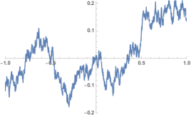
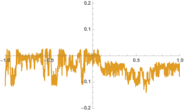
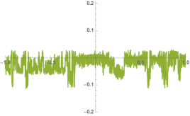
Figure 1: Simulations of $I^{{(1)}},I^{{(2)}}$ and $I^{{(3)}}$, the first three iteration of independent two-sided Brownian motions. The article studies random continuum build out the sequence of $(I^{{(n)}}:n\geq 1)$.

Continuum and pseudo-arc.

In a recent work, Kiss and Solecki used iterated Brownian motions to define a random continuum. Recall that a continuum is a nonempty, compact, connected metric space. They were interested by the so-called pseudo-arc. The pseudo-arc is a homogeneous continuum which is similar to an arc, so similar, that its existence was unclear in the beginning of the last century. A continuum $C$ is

• chainable (also called arc-like, see [15, Theorem 12.11]), if for each $\varepsilon>0$, there exists a continuous function $f:C\to[0,1]$ such that the pre-images of points under $f$ have diameter less than $\varepsilon$.

• decomposable, if there exist $A$ and $B$ two subcontinua of $C$ such that $A,B\neq C$ and $C=A\cup B$. A non decomposable continuum is called indecomposable.

• hereditarily indecomposable if any of its subcontinuum (non reduced to a singleton) is indecomposable.

By [3], the pseudo-arc is the unique (up to homeomorphisms) chainable and hereditarily indecomposable continuum non reduced to a singleton. In particular, any subcontinuum (non reduced to a singleton) of a pseudo-arc is a pseudo-arc. Its name “pseudo-arc” comes from this property because arcs have the same property, in the sense that any subcontinuum (non reduced to a singleton) of an arc is an arc. For more information on pseudo-arc, we refer the interested reader to the second paragraph of [15, Chapter XII] and to [2, 3, 12, 13]. Sadly, it is very complicated to get a “drawing” of the pseudo-arc due to its complicated crocked structure, see [15, Exercise 1.23]. Following the works of Bing, one can wonder whether the pseudo-arc is typical among arc-like continua and ask whether there is a natural probabilistic construction of the pseudo-arc.

Let us recall the construction of continua from inverse limits used in [11], see [15, Section II.2] for details. Suppose we are given a sequence

$$\cdots\xrightarrow[]{f_{3}}X_{3}\xrightarrow[]{f_{2}}X_{2}\xrightarrow[]{f_{1}}X_{1}$$

where for any $i\geq 1$, the metric space $(X_{i},d_{i})$ is compact and $f_{i}:X_{i+1}\to X_{i}$ is a continuous surjective function. Then the inverse limit of $(\{X_{i},f_{i}\})_{i\geq 1}$ is the subspace of $\prod_{i\geq 1}X_{i}$ defined by

$$\varprojlim(f_{i},X_{i}:i\geq 1)=\left\{(x_{i})_{i\geq 1}\in\prod_{i\geq 1}X_{i}:f_{i}(x_{i+1})=x_{i}\right\}.$$ (2)

In the application below $X_{i}$ are compact intervals of $\mathbb{R}$ and in this case, by [15, Theorems 2.4 and 12.19], the inverse limit is a chainable continuum. In [11], Kiss and Solecki constructed a system as above using two-sided independent Brownian motions $(\mathfrak{B}_{i}:i\geq 1)$. More precisely, they proved that for any interval $J$ of $\mathbb{R}$ with $0\in J$ and $J\neq\{0\}$, the following limit exists almost surely

$$\mathcal{I}_{i}=\lim_{m\to\infty}\mathfrak{B}_{i}\left(\mathfrak{B}_{i+1}\left(\dots\left(\mathfrak{B}_{i+m}\left(J\right)\right)\dots\right)\right),$$ (3)

and does not depend on $J$, so that we can consider the random chainable continuum $\mathcal{C}$ obtained as the inverse limit of the system

$$\cdots\xrightarrow[]{\mathfrak{B}_{3}}\mathcal{I}_{3}\xrightarrow[]{\mathfrak{B}_{2}}\mathcal{I}_{2}\xrightarrow[]{\mathfrak{B}_{1}}\mathcal{I}_{1}.$$

Kiss and Solecki proved [11, Theorem 2.1] that the random chainable continuum $\mathcal{C}$ is almost surely non-degenerate and indecomposable. This note answers negatively the obvious question the preceding result triggers:

Theorem 1.

Almost surely, the random continuum $\mathcal{C}$ is not hereditary indecomposable (hence is not the pseudo-arc).

The proof below could be adapted to prove that a random continuum constructed similarly from a sequence of i.i.d. reflected Brownian motions is neither a pseudo-arc, answering a question in [11, Section 3.1.1]. Although almost surely not homeomorphic to the pseudo-arc, the random continuum $\mathcal{C}$ is interesting in itself and one could ask about its topological property, e.g. we wonder whether the topology of $\mathcal{C}$ is almost surely constant and if it is easy to characterise.

Acknowledgements: We acknowledge support from the ERC 740943 “GeoBrown” and ANR 16-CE93-0003 “MALIN”.

2 Finding good intervals

In the rest of the article the Brownian motions $\mathfrak{B}_{i}$ are fixed and we recall the definition of $\mathcal{I}_{i}$ in (3) and of the continuum $\mathcal{C}$. We will show that Theorem 1 follows from the proposition below stated in terms of images of intervals under the flow of independent Brownian motions whose proof occupy the remaining of the article:

Proposition 2.

For any $\varepsilon>0$ small enough, with probability at least

$$p_{\varepsilon}=\prod_{i=1}^{\infty}1-2\left(\varepsilon^{{(5/4)}^{i-1}}\right)^{1/8}>0,$$

there exists two sequences $(U_{i})_{i\geq 1}$ and $(V_{i})_{i\geq 1}$ of subintervals of $\mathbb{R}$ such that, for any $i\geq 1$, the five following conditions are satisfied

1. $U_{i},V_{i}\subset\mathcal{I}_{i}$ where $\mathcal{I}_{i}$ is defined in (3),

2. $U_{i}\nsubseteq V_{i}$ and $V_{i}\nsubseteq U_{i}$,

3. $U_{i}\cap V_{i}\neq\emptyset$,

4. $U_{i}=\mathfrak{B}_{i}(U_{i+1})$ and $V_{i}=\mathfrak{B}_{i}(V_{i+1})$,

5. $|U_{i}|,|V_{i}|\leq\varepsilon^{(5/4)^{i-1}}$.

Proof of Theorem 1 given Proposition 2..

In the proof, since we are always working with the functions $\mathfrak{B}_{i}$ we write $\varprojlim(W_{i}:i\geq 1)$ for the inverse limit previously denoted by $\varprojlim(\mathfrak{B}_{i},W_{i}:i\geq 1)$ for any sequence of intervals $W_{1},W_{2},...$ such that $W_{i+1}\xrightarrow{\mathfrak{B}_{i}}W_{i}$. On the event described in the above proposition we have with probability at least $p_{\varepsilon}>0$:

• For any $i\geq 1$, $\mathfrak{B}_{i}(U_{i+1}\cup V_{i+1})=U_{i}\cup V_{i}$ (point 4) and $U_{i}\cup V_{i}\subset\mathcal{I}_{i}$ (point 1) and $U_{i}\cup V_{i}$ is an interval (point 3), so by Lemma 2.6 of [15], $\varprojlim(U_{i}\cup V_{i}:i\geq 1)$ is a subcontinuum of $\mathcal{C}$.

• By Lemma 2.6 of [15], both $\varprojlim(U_{i}:i\geq 1)$ and $\varprojlim(V_{i}:i\geq 1)$ are also subcontinua of $\varprojlim(U_{i}\cup V_{i}:i\geq 1)$.

• Let $x=(x_{i})_{i\geq 1}\in\varprojlim(U_{i}\cup V_{i}:i\geq 1)$, then

  • either, for any $i$, we have $x_{i}\in U_{i}\cap V_{i}$, and so $x\in\varprojlim(U_{i}:i\geq 1)$ and $x\in\varprojlim(V_{i}:i\geq 1)$,

  • or there exists $j\geq 1$ such that $x_{j}\in U_{j}$ and $x_{j}\notin V_{j}$, but then by point $4$ we have $x_{i}\in U_{i}$ for all $i\geq j$ and so $x\in\varprojlim(U_{i}:i\geq 1)$,

  • or there exists $j\geq 1$ such that $x_{j}\notin U_{j}$ and $x_{j}\in V_{j}$ and similarly we deduce that $x\in\varprojlim(V_{i}:i\geq 1)$.

  Hence, $\varprojlim(U_{i}\cup V_{i}:i\geq 1)\subset\varprojlim(U_{i}:i\geq 1)\cup\varprojlim(V_{i}:i\geq 1)$ and the reverse inclusion is obvious.

• $\varprojlim(U_{i}\cup V_{i}:i\geq 1)\neq\varprojlim(U_{i}:i\geq 1)$ nor $\varprojlim(U_{i}\cup V_{i}:i\geq 1)\neq\varprojlim(V_{i}:i\geq 1)$ by combining point $2$ and point 4.

All of these points imply that $\varprojlim(U_{i}\cup V_{i}:i\geq 1)$ is a decomposable subcontinuum of $\mathcal{C}=\varprojlim(\mathcal{I}_{i}:i\geq 1)$. That implies that $\mathcal{C}$ is not a pseudo-arc with probability at least $p_{\varepsilon}$ for any $\varepsilon>0$. As $p_{\varepsilon}\to 1$ when $\varepsilon\to 0$, it is not a pseudo-arc with probability one. ∎

2.1 Construction of a decomposable subcontinuum using good shape excursions

Let us now explain the idea behind the construction of the intervals of Proposition 2. This relies on the concept of excursions with a good shape. Imagine that we have a sequence of non trivial intervals $[u_{i},v_{i}]\subset[0,1]$ such that $\mathfrak{B}_{i}([u_{i+1},v_{i+1}])=[u_{i},v_{i}]$ and furthermore that $\mathfrak{B}_{i}(u_{i+1})=u_{i}$ and $\mathfrak{B}_{i}(v_{i+1})=v_{i}$ and $\mathfrak{B}_{i}(t)\in(u_{i},v_{i})$ for $t\in(u_{i+1},v_{i+1})$. In words, over the time interval $[u_{i+1},v_{i+1}]$, the Brownian motion $\mathfrak{B}_{i}$ makes an excursion from $u_{i}$ to $v_{i}$. We say that this excursion has a good shape if it stays in the pentomino of Figure 2.

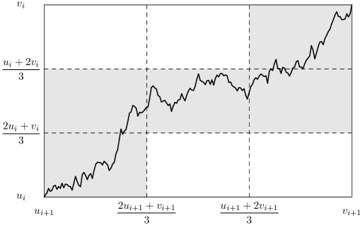
Figure 2: An excursion from $u_{i}$ to $v_{i}$ over the time interval $[u_{i+1},v_{i+1}]$ has a good shape if it stays in the light grey region.

If we have such a sequence of intervals and excursions, then one can define a sequence of intervals $U_{i},V_{i}$ by setting for any $i\geq 1$,

$$U_{i}=\lim_{n\to\infty}\underbrace{\left(\mathfrak{B}_{i}\circ\mathfrak{B}_{i+1}\circ\dots\circ\mathfrak{B}_{i+n-1}\right)\left(\left[u_{i+n},\frac{u_{i+n}+2v_{i+n}}{3}\right]\right)}_{U_{i,n}}\text{ and }$$

$$V_{i}=\lim_{n\to\infty}\left(\mathfrak{B}_{i}\circ\mathfrak{B}_{i+1}\circ\dots\circ\mathfrak{B}_{i+n-1}\right)\left(\left[\frac{2u_{i+n}+v_{i+n}}{3},v_{i+n}\right]\right).$$

First, these two limits exist a.s. and are closed intervals a.s. because they are limits of a sequence of decreasing closed intervals. Indeed, because $\mathfrak{B}_{i+n}$ performs a good shape excursion from $u_{i+n}$ to $v_{i+n}$ over $[u_{i+n+1},v_{i+n+1}]$ we have

$$\mathfrak{B}_{i+n}\left(\left[u_{i+n+1},\frac{u_{i+n+1}+2v_{i+n+1}}{3}\right]\right) \subset\left[u_{i+n},\frac{u_{i+n}+2v_{i+n}}{3}\right],\text{ and so}$$

$$U_{i,n+1} \subset U_{i,n},$$

and $U_{i,n}$ are intervals because the BM is continuous a.s. It is then an easy matter to check that the interval constructed above satisfies points 2-4 of Proposition 2. Our task is thus to construct the sequence $u_{i},v_{i}$ so that $\mathfrak{B}_{i}$ performs a good shape excursion from $u_{i}$ to $v_{i}$ over $[u_{i+1},v_{i+1}]$ and to ensure points $1$ and $5$ of Proposition 2. The key idea is to look for these intervals in the vicinity of $0$ because any given small interval close to $0$ has MANY pre-images close to $0$ by a Brownian motion. These many pre-images enable us to select one with a good shape.

2.2 Pre-images of a small interval by a Brownian motion

In the following lemma the dependence in $i$ is superfluous but we keep it to make the connection with the preceding discussion easier to understand.

Lemma 3.

Let $a_{i}$ be any real positive number small enough. Fix $[u_{i},v_{i}]\subset[0,a_{i}]$. Then with probability at least

$$1-2a_{i}^{1/8}$$

we can find $[u_{i+1},v_{i+1}]\subset[0,a_{i}^{5/4}]$ so that $\mathfrak{B}_{i}$ performs an excursion with a good shape from $u_{i}$ to $v_{i}$ over the time interval $[u_{i+1},v_{i+1}]$.

Proof.

Fix $0<u_{i}<v_{i}$ and consider the successive excursions $\mathcal{E}_{1},\mathcal{E}_{2},...$ that the Brownian motion $\mathfrak{B}_{i}$ performs from $u_{i}$ to $v_{i}$ over the respective time intervals $[u_{i+1}^{(1)},v_{i+1}^{(1)}],[u_{i+1}^{(2)},v_{i+1}^{(2)}],\cdots$. By the Markov property of Brownian motion and standard argument in excursion theory, these excursions are i.i.d. We claim that

$$r=\mathbb{P}(\mathcal{E}\mbox{ has a good shape})>0.$$

Indeed, since the law of Brownian motion has full support in the space of continuous functions (with the topology of uniform convergence over all compacts of $\mathbb{R}_{+}$), the first excursion from $u_{i}$ to $v_{i}$ might be close to any prescribed continuous function and in particular, the probability to have a good shape is strictly positive. See Figure 3.

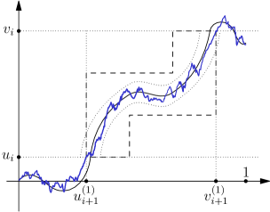
Figure 3: For any given continuous function $f$ starting from $0$ and any $\varepsilon>0$, the Brownian motion may stay within distance $\varepsilon>0$ of $f$ up to time $1$ with a positive probability. Choosing $f$ carefully, we deduce that the first excursion from $u_{i}$ to $v_{i}$ has a good shape with positive probability.

Hence, the probability that at least one of the $k$ first excursions has a good shape is at least

$$1-(1-r)^{k}.$$

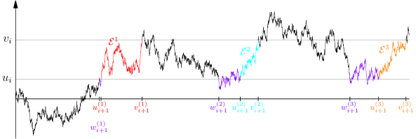
Figure 4: In red, blue and orange, the excursion from $u_{i}$ to $v_{i}$ we consider.

To control the number of excursions from $u_{i}$ to $v_{i}$ performed up to time $a_{i}$ by $\mathfrak{B}_{i}$, we introduce the auxiliary stopping times defined by $w_{i+1}^{(1)}=\inf\{t\geq 0:\mathfrak{B}_{i}(t)=u_{i}\}$ and for $k\geq 2$

$$w_{i+1}^{(k)}=\inf\{t\geq v_{i+1}^{(k-1)}:\mathfrak{B}_{i}(t)=u_{i}\}.$$

Hence $w_{i+1}^{(1)}<v_{i+1}^{(1)}<w_{i+1}^{(2)}<v_{i+1}^{(2)}<\cdots$ are the successive hitting times of $u_{i},v_{i},u_{i},v_{i}$ by $\mathfrak{B}_{i}$, see Figure 4. For $a\geq 0$, we let $\mathcal{T}_{a}=\inf\{t\geq 0:\mathfrak{B}_{i}(t)=a\}$ the hitting time of $a$ by a standard linear Brownian motion. It is classic (see e.g. [14, Theorem 2.35]) that for $a>0$ we have $\mathcal{T}_{a}=a^{2}\cdot\mathcal{T}_{1}$ in law where $\mathcal{T}_{1}$ is distributed according to the Lévy law

$$\mathcal{T}_{1}\underset{(d)}{=}\frac{\mathrm{d}t}{\sqrt{2\pi t^{3}}}\mathrm{exp}\left(-\frac{1}{2t}\right)\mathbf{1}_{t>0}.$$

In our case, applying the strong Markov property at time $w_{i+1}^{(1)}<v_{i+1}^{(1)}<w_{i+1}^{(2)}<v_{i+1}^{(2)}<\cdots$ and using invariance by symmetry we deduce that we have the equalities in distribution

$$w_{i+1}^{(1)}\stackrel{{\scriptstyle(d)}}{{=}}\mathcal{T}_{u_{i}},\quad v_{i+1}^{(1)}\stackrel{{\scriptstyle(d)}}{{=}}\mathcal{T}_{u_{i}+|v_{i}-u_{i}|},\quad w^{(2)}_{i+1}\stackrel{{\scriptstyle(d)}}{{=}}\mathcal{T}_{u_{i}+2|v_{i}-u_{i}|},\cdots,\quad v^{(k)}_{i+1}\stackrel{{\scriptstyle(d)}}{{=}}\mathcal{T}_{u_{i}+(2k-1)|v_{i}-u_{i}|},$$

for $k\geq 2$. Since $\mathcal{T}_{u_{i}+(2k-1)|v_{i}-u_{i}|}\leq\mathcal{T}_{2ka_{i}}$, the probability that the first $k$ excursions of $\mathfrak{B}_{i}$ occurs before $a_{i}^{5/4}$ is at least

$$\mathbb{P}\left(\mathcal{T}_{2ka_{i}}<a_{i}^{5/4}\right)=\mathbb{P}\left(\mathcal{T}_{1}<\left(\frac{1}{2k\,a_{i}^{3/8}}\right)\right)\geq 1-\sqrt{\frac{2}{\pi}}2ka_{i}^{3/8}\text{ (for $ka_{i}^{3/8}$ small enough)}.$$

Gathering-up the above remarks and taking $k=\lfloor a_{i}^{-1/4}\rfloor$, we deduce that the probability to do not find an excursion from $u_{i}$ to $v_{i}$ with a good shape in $[0,a_{i}^{5/4}]$ is bounded above by

$$(1-r)^{\lfloor a_{i}^{-1/4}\rfloor}+2\sqrt{\frac{2}{\pi}}\lfloor a_{i}^{-1/4}\rfloor a_{i}^{3/8}\leq 2a_{i}^{-1/8}\text{ (for $a_{i}$ small enough)}.\qed$$

3 Proof of Proposition 2

Let $(\mathfrak{B}_{i})_{i\geq 1}$ be a sequence of i.i.d. two-sided Brownian motions, and $\varepsilon$ be any real positive number small enough. For any $i\geq 1$, take $a_{i}=\varepsilon^{(5/4)^{i-1}}$.

Firstly, we put $[u_{1},v_{1}]=[0,\varepsilon]=[0,a_{1}]$, by Lemma 3, with probability at least $1-2a_{1}^{1/8}$, there exists an interval $[u_{2},v_{2}]\subset[0,a_{1}^{5/4}]=[0,a_{2}]$ such that $\mathfrak{B}_{1}$ performs a good shape excursion from $u_{1}$ to $v_{1}$ over the time interval $[u_{2},v_{2}]$. Now, we apply Lemma 3 to $[u_{2},v_{2}]\subset[0,a_{2}]$, etc. At the end, with probability at least

$$\prod_{i=1}^{\infty}1-2\left(\varepsilon^{{(5/4)}^{i-1}}\right)^{1/8},$$

we obtain a sequence of non trivial intervals $([u_{i},v_{i}])_{i\geq 1}$ such that for any $i$, $\mathfrak{B}_{i}$ makes a good shape excursion from $u_{i}$ to $v_{i}$ over $[u_{i+1},v_{i+1}]$. By Section 2.1, we can then construct two sequences of intervals $U_{i}$, $V_{i}$ that satisfy points 2-4 of Proposition 2. Moreover, by construction, $U_{i},V_{i}\subset[u_{i},v_{i}]\subset[0,a_{i}]$, hence point 5 is also satisfied.

Finally, to obtain point 1, just remark that, for any $i,n\geq 1$, $[u_{i+n},v_{i+n}]\subset[0,a_{i+n}]\subset[0,1]$, so

$$U_{i} =\lim_{n\to\infty}\left(\mathfrak{B}_{i}\circ\mathfrak{B}_{i+1}\circ\dots\circ\mathfrak{B}_{i+n}\right)\left(\left[u_{i+n+1},\frac{u_{i+n+1}+2v_{i+n+1}}{3}\right]\right)$$

$$\subset\lim_{n\to\infty}\left(\mathfrak{B}_{i}\circ\mathfrak{B}_{i+1}\circ\dots\circ\mathfrak{B}_{i+n}\right)\left(\left[0,1\right]\right)=\mathcal{I}_{i}\text{ (by\leavevmode\nobreak\ \eqref{eq:interval})}.$$

Similarly, $V_{i}\subset\mathcal{I}_{i}$. ∎

References

- [1] Jean Bertoin. Iterated Brownian motion and stable(1/4) subordinator. Statistics & probability letters, 27(2):111–114, 1996.
- [2] R. H. Bing. A homogeneous indecomposable plane continuum. Duke Mathematical Journal, 15(3):729–742, 1948.
- [3] R. H. Bing. Concerning hereditarily indecomposable continua. Pacific Journal of Mathematics, 1(1):43–51, 1951.
- [4] Krzysztof Burdzy. Some path properties of iterated Brownian motion. In Seminar on Stochastic Processes, 1992, pages 67–87. Springer, 1993.
- [5] Krzysztof Burdzy and Davar Khoshnevisan. The level sets of iterated Brownian motion. In Séminaire de Probabilités XXIX, pages 231–236. Springer, 1995.
- [6] Jérôme Casse and Jean-François Marckert. Processes iterated ad libitum. Stochastic Processes and their Applications, 126(11):3353–3376, 2016.
- [7] Nicolas Curien and Takis Konstantopoulos. Iterating Brownian motions, ad libitum. Journal of theoretical probability, 27(2):433–448, 2014.
- [8] Nathalie Eisenbaum and Zhan Shi. Uniform oscillations of the local time of iterated Brownian motion. Bernoulli, 5(1):49–65, 1999.
- [9] Tadahisa Funaki. Probabilistic construction of the solution of some higher order parabolic differential equation. Proceedings of the Japan Academy, Series A, Mathematical Sciences, 55(5):176–179, 1979.
- [10] Davar Khoshnevisan and Thomas M Lewis. Iterated Brownian motion and its intrinsic skeletal structure. In Seminar on Stochastic Analysis, Random Fields and Applications, pages 201–210. Springer, 1999.
- [11] Viktor Kiss and Sławomir Solecki. Random continuum and Brownian motion. arXiv preprint arXiv:2004.01367, 2020.
- [12] Bronisław Knaster. Un continu dont tout sous-continu est indécomposable. Fundamenta Mathematicae, 1(3):247–286, 1922.
- [13] Edwin E. Moise. An indecomposable plane continuum which is homeomorphic to each of its nondegenerate subcontinua. Transactions of the American Mathematical Society, 63(3):581–594, 1948.
- [14] Peter Mörters and Yuval Peres. Brownian motion, volume 30. Cambridge University Press, 2010.
- [15] Sam Nadler. Continuum theory: an introduction. CRC Press, 1992.
- [16] Enzo Orsingher and Luisa Beghin. Fractional diffusion equations and processes with randomly varying time. The Annals of Probability, pages 206–249, 2009.
- [17] Yimin Xiao. Local times and related properties of multidimensional iterated Brownian motion. Journal of Theoretical Probability, 11(2):383–408, 1998.