Chaos in the Bose-glass phase of a one-dimensional disordered Bose fluid

Abstract

We show that the Bose-glass phase of a one-dimensional disordered Bose fluid exhibits a chaotic behavior, i.e., an extreme sensitivity to external parameters. Using bosonization, the replica formalism and the nonperturbative functional renormalization group, we find that the ground state is unstable to any modification of the disorder configuration (“disorder” chaos) or variation of the Luttinger parameter (“quantum” chaos, analog to the “temperature” chaos in classical disordered systems). This result is obtained by considering two copies of the system, with slightly different disorder configurations or Luttinger parameters, and showing that inter-copy statistical correlations are suppressed at length scales larger than an overlap length $\xi_{\rm ov}\sim|\epsilon|^{-1/\alpha}$ ($|\epsilon|\ll 1$ is a measure of the difference between the disorder distributions or Luttinger parameters of the two copies). The chaos exponent $\alpha$ can be obtained by computing $\xi_{\rm ov}$ or by studying the instability of the Bose-glass fixed point for the two-copy system when $\epsilon\neq 0$. The renormalized, functional, inter-copy disorder correlator departs from its fixed-point value – characterized by cuspy singularities – via a chaos boundary layer, in the same way as it approaches the Bose-glass fixed point when $\epsilon=0$ through a quantum boundary layer. Performing a linear analysis of perturbations about the Bose-glass fixed point, we find $\alpha=1$.

I Introduction

In a Bose fluid with short-range interactions, disorder can induce a quantum phase transition between a superfluid phase and a localized phase dubbed Bose glass (BG).Giamarchi and Schulz (1987, 1988); Fisher et al. (1989) The latter is characterized by a nonzero compressibility, a vanishing dc conductivity and the absence of gap in the optical conductivity. As its name indicates, the BG phase is expected to be analogous to the Fermi-glass phase of interacting fermions in a strong disorder potential and exhibit some of the characteristic properties of glassy systems.Fisher et al. (1989)

In one dimension, the analogy of the BG phase with other disordered systems exhibiting glassy properties is strongly supported by the nonperturbative functional renormalization group (FRG).Dupuis (2019); Dupuis and Daviet (2020); Dupuis (2020); Daviet and Dupuis (2020) In this approach, one finds that the BG phase is described by an attractive fixed point analog to the zero-temperature fixed point controlling the low-temperature phase of many classical disordered systems. The role of temperature is played by the Luttinger parameter $K\sim k^{\theta}$ which, as the momentum scale $k$ approaches zero, vanishes with an exponent $\theta=z-1$ related to the dynamical critical exponent $z$. Moreover, the renormalized disorder correlator assumes a cuspy functional form associated with the existence of metastable states.Balents et al. (1996) At nonzero momentum scale, quantum tunneling between the ground state and these metastable states leads to a rounding of the cusp singularity into a quantum boundary layer (QBL). The latter controls the low-energy dynamics and is responsible for the $\omega^{2}$ behavior of the (dissipative) conductivity. Thus the FRG approach reveals some of the glassy properties (pinning, “shocks” or static avalanches) of the BG phase and, to some extent, can be understood within the “droplet” pictureFisher and Huse (1988a) put forward for the description of glassy (classical) systems.Dupuis and Daviet (2020)

One of the peculiar features of glassy systems is the extreme sensitivity of the ground state with respect to small changes in external parameters like the disorder configuration or the temperature. In some cases, an infinitesimal perturbation is sufficient to lead to a complete reorganization of the ground state at large length scales. This situation is referred to as chaos,McKay et al. (1982); Bray and Moore (1987); Fisher and Huse (1988b, 1991); Shapir (1991); Kondor and Vegso (1993); Kisker and Rieger (1998) e.g. disorder chaos or temperature chaos according to the external parameter being considered. Chaos is usually characterized by an overlap length $\xi_{\rm ov}$ beyond which the ground state completely changes as a result of the variation in the external parameter. The overlap length diverges as $\xi_{\rm ov}\sim|\epsilon|^{-1/\alpha}$ where $\alpha$ is called the chaos exponent ($|\epsilon|\ll 1$ is a measure of the change in the external parameter). Although chaos was originally predicted for spin glasses, it is also characteristic of elastic manifolds pinned by disorder where the long-distance physics is controlled by a zero-temperature fixed point.Shapir (1991); Le Doussal (2006); Duemmer and Le Doussal (2007) To our knowledge, the only quantum disordered system where (disorder) chaos was studied is the two-dimensional Anderson insulator.Lemarié (2019)

In this paper, we study chaos in the BG phase of a one-dimensional Bose fluid. In Sec. II we briefly recall the FRG formalism used in Refs. Dupuis, 2019; Dupuis and Daviet, 2020 to study the BG phase and generalize it to include two copies of the system subjected to slightly different disorder configurations.not (a) In particular we introduce the main quantities of interest: the running Luttinger parameter $K_{k}$ and the intra- and inter-copy renormalized disorder correlators, $\delta_{11,k}(u)=\delta_{22,k}(u)$ and $\delta_{12,k}(u)$ respectively. Here $k$ is a running momentum scale and $u\equiv\phi_{a}-\phi_{b}$ stands for the difference between the fields in two different replicas. The flow equations for $K_{k}$ and $\delta_{ij,k}(u)$ are similar to those obtained for pinned disordered periodic manifolds by Duemmer and Le Doussal (DLD) in Refs. Le Doussal, 2006; Duemmer and Le Doussal, 2007, with $K_{k}$ playing the role of the temperature.

In section III.1 we first consider the approach to the BG fixed point when the two copies are identical (i.e., experience the same disorder potential: $\epsilon=0$). In that case, the $\pi$-periodic functions $\delta_{ii,k}(u)$ and $\delta_{12,k}(u)$ approach a fixed-point function $\delta^{*}(u)$ exhibiting cusps at $u=p\pi$ ($p$ integer). At nonzero momentum scale the cusp singularity at $u=p\pi$ is rounded into a QBL. A linear analysis of the perturbations about $\delta^{*}(u)$ shows that the less irrelevant eigenvalue $\lambda=-\theta$ is associated with an eigenfunction which is increasingly peaked around $u=p\pi$ as the number $n_{\rm max}$ of circular harmonics of $\delta_{ij,k}(u)$ (used in the numerical solution of the linearized flow equations) increases, whereas all other eigenfunctions remain extended over the whole interval $[0,\pi]$.

In Sec. III.2 we show that the BG fixed point is unstable for any nonzero $\epsilon$ since in that case $\delta_{ii,k}(u)\to\delta^{*}(u)$ but $\delta_{12,k}(u)\to 0$ in the limit $k\to 0$. Thus the two copies become statistically independent in the large-distance limit, which corresponds to disorder chaos. From the numerical solution of the flow equations we find that $\delta_{12,k}(0)$ satisfies a scaling form with a characteristic length $\xi_{\rm ov}\sim|\epsilon|^{-1/\alpha}$ but the chaos exponent $\alpha$ seems to converge very slowly with $n_{\rm max}$. The instability of the BG fixed point occurs via a chaos boundary layerLe Doussal (2006); Duemmer and Le Doussal (2007) (CBL) reminiscent of the QBL observed in the approach to the BG fixed point. The linear analysis of the perturbations about the fixed-point solution $\delta^{*}(u)$ reveals a single positive eigenvalue $\lambda\equiv 2\alpha$ associated with a function which is increasingly peaked around $u=p\pi$ as $n_{\rm max}$ increases. The convergence of $\alpha$ with $n_{\rm max}$ is extremely slow but in the limit $n_{\rm max}\to\infty$ the solution can be found analytically (and is essentially given by a Dirac comb) and yields the chaos exponent $\alpha=1$. We are then able to show that the convergence of $\alpha$ with $n_{\rm max}$ is logarithmic. The agreements and differences between our results and those of DLD are discussed in Sec. III.2.4. Finally, in Sec. IV, we show that chaos is also obtained when one considers a slight change in the Luttinger parameter.

II Model and FRG formalism

We consider a one-dimensional Bose fluid described by the Hamiltonian $\hat{H}_{0}$. At low energies $\hat{H}_{0}$ can be approximated by the Tomonaga-Luttinger HamiltonianGiamarchi (2004); Haldane (1981); Cazalilla et al. (2011)

$$\hat{H}_{0}=\int dx\frac{v}{2\pi}\left\{\frac{1}{K}(\partial_{x}\hat{\varphi})^{2}+K(\partial_{x}\hat{\theta})^{2}\right\},$$ (1)

where $\hat{\theta}$ is the phase of the boson operator $\hat{\psi}(x)=e^{i\hat{\theta}(x)}\hat{\rho}(x)^{1/2}$ and $\hat{\varphi}$ is related to the density operator via

$$\hat{\rho}(x)=\rho_{0}-\frac{1}{\pi}\partial_{x}\hat{\varphi}(x)+2\rho_{2}\cos(2\pi\rho_{0}x-2\hat{\varphi}(x)),$$ (2)

where $\rho_{0}$ is the average density and $\rho_{2}$ a nonuniversal parameter that depends on microscopic details. $\hat{\varphi}$ and $\hat{\theta}$ satisfy the commutation relations $[\hat{\theta}(x),\partial_{y}\hat{\varphi}(y)]=i\pi\delta(x-y)$. $v$ denotes the sound-mode velocity and the dimensionless parameter $K$, which encodes the strength of boson-boson interactions, is the Luttinger parameter. The ground state of $\hat{H}_{0}$ is a Luttinger liquid, i.e., a superfluid state with superfluid stiffness $\rho_{s}=vK/\pi$ and compressibility $\kappa=d\rho_{0}/d\mu=K/\pi v$.Giamarchi (2004)

The disorder contributes to the Hamiltonian a termGiamarchi and Schulz (1987, 1988)

$$\hat{H}_{\rm dis}=\int dx\left\{-\frac{1}{\pi}\eta\partial_{x}\hat{\varphi}+\rho_{2}[\xi^{*}e^{2i\hat{\varphi}}+{\rm h.c.}]\right\},$$ (3)

where $\eta(x)$ (real) and $\xi(x)$ (complex) denote random potentials with Fourier components near 0 and $\pm 2\pi\rho_{0}$, respectively. $\eta$ can be eliminated by a shift of $\hat{\varphi}$ and is not considered in the following.Dupuis and Daviet (2020)

In the functional-integral formalism, after integrating out the field $\theta$, one obtains the Euclidean (imaginary-time) action

$$S[\varphi;\xi]={} \int_{X}\biggl{\{}\frac{v}{2\pi K}\left[(\partial_{x}\varphi)^{2}+v^{-2}({\partial_{\tau}}\varphi)^{2}\right]$$

$$+\rho_{2}[\xi^{*}e^{2i\varphi}+{\rm c.c.}]\biggr{\}},$$ (4)

where we use the notation $X=(x,\tau)$, $\int_{X}=\int_{0}^{\beta}d\tau\int dx$ and $\varphi(X)$ is a bosonic field with $\tau\in[0,\beta]$. The model is regularized by a UV cutoff $\Lambda$ acting both on momenta and frequencies. We shall only consider the zero-temperature limit $\beta=1/T\to\infty$ but $\beta$ will be kept finite at intermediate stages of calculations.

II.1 Introducing two copies and $n$ replicas

To investigate the chaotic nature of the BG phase, we consider two copies of the system with slightly different realizations of the disorder,

$$\begin{split}\xi_{1}(x)&=\xi(x)+\epsilon\zeta(x),\\ \xi_{2}(x)&=\xi(x)-\epsilon\zeta(x),\end{split}$$ (5)

where $|\epsilon|\ll 1$. The random potentials $\xi$ and $\zeta$ are uncorrelated and identically distributed, i.e., assuming Gaussian distributions with zero mean,

$$\begin{split}&\overline{\xi(x)}=\overline{\zeta(x)}=0,\\ &\overline{\xi^{*}(x)\xi(x^{\prime})}=\overline{\zeta^{*}(x)\zeta(x^{\prime})}=D\delta(x-x^{\prime})\end{split}$$ (6)

(all other correlators, e.g. $\overline{\xi(x)\xi(x^{\prime})}$, vanish). We use an overline to denote disorder averaging. Equations (6) imply

$$\begin{split}&\overline{\xi^{*}_{i}(x)\xi_{j}(x^{\prime})}=D_{ij}\delta(x-x^{\prime}),\\ &D_{ii}=D(1+\epsilon^{2}),\quad D_{12}=D_{21}=D(1-\epsilon^{2}).\end{split}$$ (7)

The statistical correlations between the two systems are characterized by the correlation functions

$$C_{ij}(X-X^{\prime})=\overline{\langle(\varphi_{i}(X)-\varphi_{i}(X^{\prime}))(\varphi_{j}(X)-\varphi_{j}(X^{\prime}))\rangle}.$$ (8)

Since the two copies are independent before disorder averaging,

$$\begin{split}C_{ii}(X-X^{\prime})={}&2[G_{c,ii}(0)+G_{d,ii}(0)\\ &-G_{c,ii}(X-X^{\prime})-G_{d,ii}(X-X^{\prime})],\\ C_{12}(X-X^{\prime})={}&2[G_{d,12}(0)-G_{d,12}(X-X^{\prime})],\end{split}$$ (9)

where

$$\begin{split}G_{c,ij}(X-X^{\prime})&=\overline{\langle\varphi_{i}(X)\varphi_{j}(X^{\prime})\rangle}-\overline{\langle\varphi_{i}(X)\rangle\langle\varphi_{j}(X^{\prime})\rangle},\\ G_{d,ij}(X-X^{\prime})&=\overline{\langle\varphi_{i}(X)\rangle\langle\varphi_{j}(X^{\prime})\rangle}-\overline{\langle\varphi_{i}(X)\rangle}\;\overline{\langle\varphi_{j}(X^{\prime})\rangle}\end{split}$$ (10)

are the connected and disconnected propagators, respectively. The long-distance part of both $C_{ii}(X-X^{\prime})$ and $C_{12}(X-X^{\prime})$ is determined by $G_{d,ij}(X-X^{\prime})$.Dupuis and Daviet (2020)

In the replica formalism, one considers $n$ replicas of the system and the disorder-averaged partition function

$${\cal Z}[\{J_{ia}\}]=\overline{\prod_{a=1}^{n}\prod_{i=1}^{2}{\cal Z}[J_{ia};\xi_{i}]},$$ (11)

where the $2n$ external sources $\{J_{ia}\}$ act on each replica independently and

$${\cal Z}[J_{ia};\xi_{i}]=\int{\cal D}[\varphi_{ia}]\,e^{-S[\varphi_{ia},\xi_{i}]+\int_{X}J_{ia}(X)\varphi_{ia}(X)}$$ (12)

is the partition function of the $a$th replica of the $i$th copy before disorder averaging. Using (7) to perform the disorder average, one obtains

$${\cal Z}[\{J_{ia}\}]=\int{\cal D}[\{\varphi_{ia}\}]\,e^{-S[\{\varphi_{ia}\}]+\sum_{a,i}\int_{X}J_{ia}(X)\varphi_{ia}(X)},$$ (13)

with the replicated action

$$S[\{\varphi_{ia}\}]=\sum_{i,a}\int_{x,\tau}\frac{v}{2\pi K}\left\{(\partial_{x}\varphi_{ia})^{2}+\frac{({\partial_{\tau}}\varphi_{ia})^{2}}{v^{2}}\right\}\\ -\sum_{a,b,i,j}{\cal D}_{ij}\int_{x,\tau,\tau^{\prime}}\cos[2\varphi_{ia}(x,\tau)-2\varphi_{jb}(x,\tau^{\prime})],$$ (14)

where ${\cal D}_{ij}=\rho_{2}^{2}D_{ij}$.

II.2 Effective action and FRG

To implement the nonperturbative FRG approach,Berges et al. (2002); Kopietz et al. (2010); Delamotte (2012); Dupuis et al. (2021) we add to the action (14) the infrared regulator termDupuis and Daviet (2020)

$$\Delta S_{k}[\{\varphi_{ia}\}]=\frac{1}{2}\sum_{i,a,q,\omega}\varphi_{ia}(-q,-i\omega)R_{k}(q,i\omega)\varphi_{ia}(q,i\omega),$$ (15)

where $k$ is a (running) momentum scale varying from the UV scale $\Lambda$ down to zero and $\omega\equiv\omega_{n}=2\pi n/\beta$ ($n$ integer) is a Matsubara frequency. The cutoff function $R_{k}(q,i\omega)$ is chosen so that fluctuation modes satisfying $|q|,|\omega|/v_{k}\ll k$ are suppressed while those with $|q|\gg k$ or $|\omega|/v_{k}\gg k$ are left unaffected (the $k$-dependent sound-mode velocity $v_{k}$ is defined below). In practice we choose

$$R_{k}(q,i\omega)=Z_{x}\left(q^{2}+\frac{\omega^{2}}{v_{k}^{2}}\right)r\left(\frac{q^{2}+\omega^{2}/v_{k}^{2}}{k^{2}}\right),$$ (16)

where $r(y)=\alpha/(e^{y}-1)$ with $\alpha$ a constant of order unity. $Z_{x}$ is defined below.

The partition function

$${\cal Z}_{k}[\{J_{ia}\}]={} \int{\cal D}[\{\varphi_{ia}\}]\exp\Bigl{\{}-S[\{\varphi_{ia}\}]$$

$$-\Delta S_{k}[\{\varphi_{ia}\}]+\sum_{i,a}\int_{X}J_{ia}\varphi_{ia}\Bigr{\}}$$ (17)

thus becomes $k$ dependent. The expectation value of the field reads

$$\phi_{ia}(X)=\frac{\delta\ln{\cal Z}_{k}[\{J_{jf}\}]}{\delta J_{ia}(X)}=\langle\varphi_{ia}(X)\rangle$$ (18)

(to avoid confusion in the indices we denote by $\{J_{jf}\}$ the $2n$ external sources).

The scale-dependent effective action

$$\Gamma_{k}[\{\phi_{ia}\}]=-\ln{\cal Z}_{k}[\{J_{ia}\}]+\sum_{i,a}\int_{X}J_{ia}\phi_{ia}-\Delta S_{k}[\{\phi_{ia}\}]$$ (19)

is defined as a modified Legendre transform which includes the subtraction of $\Delta S_{k}[\{\phi_{ia}\}]$. Assuming that for $k=\Lambda$ the fluctuations are completely frozen by the term $\Delta S_{\Lambda}$, $\Gamma_{\Lambda}[\{\phi_{ia}\}]=S[\{\phi_{ia}\}]$. On the other hand the effective action of the original model (14) is given by $\Gamma_{k=0}$ since $R_{k=0}$ vanishes. The nonperturbative FRG approach aims at determining $\Gamma_{k=0}$ from $\Gamma_{\Lambda}$ using Wetterich’s equationWetterich (1993); Ellwanger (1994); Morris (1994)

$$\partial_{t}\Gamma_{k}[\{\phi_{ia}\}]=\frac{1}{2}{\rm Tr}\left\{\partial_{t}R_{k}\bigl{(}\Gamma_{k}^{(2)}[\{\phi_{ia}\}]+R_{k}\bigr{)}^{-1}\right\},$$ (20)

where $\Gamma_{k}^{(2)}$ is the second functional derivative of $\Gamma_{k}$ and $t=\ln(k/\Lambda)$ a (negative) RG “time”. The trace in (20) involves a sum over momenta and frequencies as well as copy and replica indices.

To solve (approximately) the flow equation (20) we consider the following ansatz for the effective actionDupuis (2019); Dupuis and Daviet (2020)

$$\Gamma_{k}[\{\phi_{ia}\}]=\sum_{a}\Gamma_{1,k}[\phi_{a}]-\frac{1}{2}\sum_{a,b}\Gamma_{2,k}[\phi_{a},\phi_{b}],$$ (21)

where $\phi_{a}=\{\phi_{1a},\phi_{2a}\}$ and

$$\Gamma_{1,k}[\phi_{a}]=\sum_{i}\int_{X}\frac{Z_{x}}{2}\left\{(\partial_{x}\phi_{ia})^{2}+\frac{({\partial_{\tau}}\phi_{ia})^{2}}{v_{k}^{2}}\right\},$$

$$\Gamma_{2,k}[\phi_{a},\phi_{b}]=\sum_{i,j}\int_{x,\tau,\tau^{\prime}}V_{ij,k}\bigl{(}\phi_{ia}(x,\tau)-\phi_{jb}(x,\tau^{\prime})\bigr{)},$$ (22)

with initial conditions $Z_{x}=v/\pi K$, $v_{\Lambda}=v$ and $V_{\Lambda,ij}(u)=2{\cal D}_{ij}\cos(2u)$. The form of $\Gamma_{1,k}$ and $\Gamma_{2,k}$ is strongly constrained by the statistical tilt symmetry (STS) due to the invariance of the disorder part of the action (14) in the time-independent shift $\varphi_{ia}(X)\to\varphi^{\prime}_{ia}(X)=\varphi_{ia}(X)+w(x)$ with $w(x)$ an arbitrary function of $x$.Dupuis and Daviet (2020) The STS yields

$$\Gamma_{k}[\{\phi^{\prime}_{ia}\}]={} \Gamma_{k}[\{\phi_{ia}\}]+n\beta Z_{x}\int_{x}(\partial_{x}w)^{2}$$

$$+Z_{x}\sum_{i,a}\int_{X}(\partial_{x}w)(\partial_{x}\phi_{ia}).$$ (23)

This implies that $Z_{x}$ remains equal to its initial value and no other space derivative terms are allowed; for instance the term $(\partial_{x}\phi_{1a})(\partial_{x}\phi_{2a})$ is not possible. The term $({\partial_{\tau}}\phi_{1a})({\partial_{\tau}}\phi_{2a})$ is a priori not excluded by the STS but is not generated by the flow equation. Since the two copies are equivalent (${\cal D}_{11}={\cal D}_{22}$), the velocity $v_{k}$ is copy independent. In addition to $v_{k}$ one may define a $k$-dependent Luttinger parameter by $Z_{x}=v_{k}/\pi K_{k}$. The STS also ensures that the two-replica potential $V_{ij,k}(\phi_{ia},\phi_{jb})$ is a function of $\phi_{ia}-\phi_{jb}$ only.

Thus the main quantities of interest are $K_{k}$, $v_{k}$ and the two-replica potential $V_{ij,k}(u)$. It is convenient to introduce the dimensionless function

$$\delta_{ij,k}(u)=-\frac{K^{2}}{v^{2}}\frac{V_{ij,k}^{\prime\prime}(u)}{k^{3}}.$$ (24)

For a single copy, the BG fixed point is characterized by a vanishing of $K_{k}$ and $v_{k}$: $K_{k},v_{k}\sim k^{\theta}$ for $k\to 0$. The vanishing of $K_{k}$ implies that quantum fluctuations are suppressed at low energies and therefore a pinning of the field $\varphi(x,\tau)$ by the random potential. On the other hand the $\pi$-periodic function $\delta^{*}(u)=\lim_{k\to 0}\delta_{k}(u)$ exhibits cusps at $u=p\pi$ ($p$ integer). This cuspy nonanalytic form is related to the existence of metastable states.Balents et al. (1996) At nonzero momentum scale, quantum tunneling between the ground state and these metastable states leads to a rounding of the nonanalyticity into a QBL. The latter is responsible for the vanishing of the optical conductivity $\sigma(\omega)\sim\omega^{2}$ in the low-frequency limit.Dupuis (2019); Dupuis and Daviet (2020)

With the ansatz (21,22), the disconnected propagator of the two-copy system is given by

$$G_{d,ij,k}(q,i\omega)=\beta\delta_{\omega,0}\frac{v^{2}k^{3}}{K^{2}}\frac{\delta_{ij,k}(0)}{[Z_{x}q^{2}+R_{k}(q,0)]^{2}}.$$ (25)

Stricto sensu this expression is valid only for $|q|\ll k$ since the ansatz (21,22) is based on a derivative expansion. However, we expect $q$ to act as an infrared cutoff in the flow so that $G_{d,ij,k=0}(q,0)$ can be approximately obtained by setting $k\sim|q|$, i.e.,

$$G_{d,ij,k=0}(q,i\omega)\sim\beta\delta_{\omega,0}\frac{\pi^{2}\delta_{ij,|q|}(0)}{|q|}.$$ (26)

Since the intracopy correlation function $C_{ii}(X)$ is not modified by the inter-copy statistical correlations, we have $C_{ii}(X)\simeq 2\pi\delta^{*}(0)\ln|x|$.Dupuis and Daviet (2020) The system exhibits chaos if $\lim_{x\to\infty}C_{12}(X)=0$ for any $\epsilon>0$, which requires $\lim_{k\to 0}\delta_{12,k}(0)=0$: The two copies are then statistically independent at long distances regardless of the (nonzero) difference in the random potentials $\xi_{1}(x)$ and $\xi_{2}(x)$. In the following we shall therefore consider the flow of

$$F_{k}=\frac{1+\epsilon^{2}}{1-\epsilon^{2}}\frac{\delta_{12,k}(0)}{\frac{1}{2}[\delta_{11,k}(0)+\delta_{22,k}(0)]},$$ (27)

with initial condition $F_{\Lambda}=1$.

II.3 Flow equations

A detailed derivation of the flow equations for a single copy can be found in Ref. Dupuis and Daviet, 2020. The generalization to two copies is straightforward and gives

$$\partial_{t}\delta_{ii,k}(u)={} -3\delta_{ii,k}(u)-l_{1}K_{k}\delta^{\prime\prime}_{ii,k}(u)$$

$$+\pi\bar{l}_{2}\{\delta_{ii,k}^{\prime\prime}(u)[\delta_{ii,k}(u)-\delta_{ii,k}(0)]+\delta^{\prime}_{ii,k}(u)^{2}\},$$ (28)

$$\partial_{t}\delta_{12,k}(u)={} -3\delta_{12,k}(u)-l_{1}K_{k}\delta^{\prime\prime}_{12,k}(u)$$

$$+\pi\bar{l}_{2}\{\delta_{12,k}^{\prime\prime}(u)[\delta_{12,k}(u)-\delta_{ii,k}(0)]+\delta^{\prime}_{12,k}(u)^{2}\},$$ (29)

and

$$\partial_{t}K_{k}=\theta_{k}K_{k},\qquad\partial_{t}(K_{k}/v_{k})=0,$$ (30)

where

$$\theta_{k}=z_{k}-1=\frac{\pi}{2}\delta^{\prime\prime}_{ii,k}(0)\bar{m}_{\tau}$$ (31)

with $z_{k}$ being the running dynamical critical exponent. The thresholds functions $l_{1}$, $\bar{l}_{2}$ and $\bar{m}_{\tau}$ are defined in Ref. Dupuis and Daviet, 2020. Note that the $\pi$ periodicity of $\delta_{ij,k}(u)$, as well as the property $\int_{0}^{\pi}du\,\delta_{ij,k}(u)=0$, are maintained by the flow equations.

III Disorder chaos

We consider only the case where the parameters of the microscopic action (i.e., the initial conditions of the RG flow) are such that the system is in the BG phase. The flow equations are integrated numerically using the fourth-order Runge-Kutta method with adaptative step size. The functions

$$\delta_{ij,k}(u)=\sum_{n=1}^{n_{\rm max}}\delta_{ij,n,k}\cos(2nu)$$ (32)

are expanded in circular harmonics with $n_{\rm max}$ in the range $[100-800]$. Note that $\delta_{ij,0,k}$ necessary vanishes since $\int_{0}^{\pi}du\,\delta_{ij,k}(u)=0$.

III.1 Approach to the BG fixed point

As expected, the RG equations for $\delta_{ii,k}(u)$, $K_{k}$ and $v_{k}$ are identical to the one-copy case.Dupuis and Daviet (2020) The function $\delta_{ii,k}(u)$ approaches the $\pi$-periodic fixed-point solution

$$\delta^{*}(u)=\frac{1}{2\pi\bar{l}_{2}}\left[\left(u-\frac{\pi}{2}\right)^{2}-\frac{\pi^{2}}{12}\right],\quad u\in[0,\pi],$$ (33)

which exhibits cusps at $u=p\pi$ ($p$ integer). The BG fixed point is a “critical”, scale-invariant, fixed point as far as the disorder correlator $\delta_{ii,k}(u)$ is concerned, i.e., in the zero-frequency sector. The finite localization length, which characterizes the BG phase, appears only in the nonzero-frequency sector of the theory, a feature which is related to the nonanalytic structure of the propagator at zero frequency.Dupuis and Daviet (2020)

III.1.1 Quantum boundary layer

For any nonzero momentum scale $k$, the cusp singularity at $u=p\pi$ is rounded into a boundary layer. In the vicinity of the BG fixed point, $K_{k}\to 0$, the solution can be written in the form

$$\delta_{ii,k}(u)=\delta_{ii,k}(0)+K_{k}f\left(\frac{u}{K_{k}}\right)$$ (34)

near $u=0$ and for an arbitrary value of the ratio $u/K_{k}$. The $k$-independent even function satisfies $f(0)=f^{\prime}(0)=0$ and $f^{\prime\prime}(0)<0$. From (28) we obtain

$$\partial_{t}\delta_{ii,k}(0)\simeq-3\delta_{ii,k}(0)-l_{1}f^{\prime\prime}+\pi\bar{l}_{2}(f^{\prime\prime}f+f^{\prime}{}^{2})$$ (35)

using $K_{k}\to 0$ and $\partial_{t}K_{k}=\theta_{k}K_{k}\to 0$. The right-hand side must be independent of $x=u/K_{k}$ and equal to $-3\delta_{ii,k}(0)-l_{1}f^{\prime\prime}(0)$ since $f(0)=f^{\prime}(0)=0$, i.e.,

$$-l_{1}f^{\prime\prime}+\pi\bar{l}_{2}(f^{\prime\prime}f+f^{\prime}{}^{2})=-l_{1}f^{\prime\prime}(0).$$ (36)

This yields

$$f(x)=\frac{l_{1}}{\pi\bar{l}_{2}}\left\{1-\left[1-\frac{\pi\bar{l}_{2}}{l_{1}}f^{\prime\prime}(0)x^{2}\right]^{1/2}\right\}.$$ (37)

Since the solution (34) must approach the fixed-point solution $\delta^{*}(u)$ when $K_{k}\to 0$, we deduce $f^{\prime\prime}(0)=-\pi/4l_{1}\bar{l}_{2}$.

From (35) and (36) we also obtain

$$\partial_{t}\delta_{ii}(0)=-3\delta_{k,ii}(0)-l_{1}f^{\prime\prime}(0),$$ (38)

i.e.,

$$\delta_{ii,k}(0)=Ce^{-3t}-\frac{l_{1}}{3}f^{\prime\prime}(0).$$ (39)

Since $\delta_{11,k}(0)$ approaches a finite value as $t\to-\infty$, the constant $C$ must necessarily vanish. From the flow equation (28) it is easy to see that the relevant eigenvalue 3 is associated with a constant solution $\delta_{k}(u)={\rm const}$, which is not allowed as it violates the condition $\int_{0}^{\pi}du\,\delta_{ii,k}(u)=0$. We therefore obtain

$$\delta_{ii,k}(0)=-\frac{l_{1}}{3}f^{\prime\prime}(0)=\frac{\pi}{12\bar{l}_{2}}=\delta^{*}(0),$$ (40)

which is the expected result in the limit $k\to 0$. For $k>0$, we expect

$$\delta_{ii,k}(0)=\delta^{*}(0)-\frac{l_{1}}{\pi\bar{l}_{2}}K_{k}$$ (41)

to leading order in $K_{k}$,not (b) where the prefactor of $K_{k}$ is determined by requiring that $\delta_{ii,k}(u)-\delta^{*}(u)$ vanishes to order $K_{k}$ when $|u|/K_{k}\gg 1$. The QBL defined by (34,37,41) is in very good agreement with the numerical solution of the flow equations (see the discussion of the QBL and CBL in Sec. III.2.2 and Fig. 5).

The preceding results imply the deviation from the BG fixed point

$$g_{k}(u) =\delta_{ii,k}(u)-\delta^{*}(u)$$

$$\simeq\left\{\begin{array}[]{lll}-\frac{l_{1}}{\pi\bar{l}_{2}}K_{k}+\frac{|u|}{2\bar{l}_{2}}&\mbox{if}&|u|\ll K_{k},\\ 0&\mbox{if}&|u|\gg K_{k}.\end{array}\right.$$ (44)

We conclude that when $K_{k}\to 0$ (i.e., $k\to 0$) the function $g_{k}(u)$, which characterizes the approach to the BG fixed point via the QBL, tends to $\sim K_{k}\mbox{\tencyr SH}^{(K)}_{u,0}$ where $\mbox{\tencyr SH}^{(K)}_{u,0}$ is the $\pi$-periodic Kronecker comb.not (c) In the next section we shall see how this result can be reproduced from a linear analysis of the perturbations about the fixed point.

III.1.2 Linear analysis

Let us consider a small perturbation about the BG fixed point $(K^{*}=0,\delta^{*}(u))$,

$$\begin{split}\delta_{ii,k}(u)&=\delta^{*}(u)+g(u)e^{-\lambda t},\\ K_{k}&=K^{*}+Ke^{-\lambda t},\end{split}$$ (45)

where $g(u)$ and $K$ (not to be confused with the bare value $K_{\Lambda}$ of the Luttinger parameter) are $k$ independent. To first order in $g$ and $K$, we obtain the flow equations

$$\lambda g(u)={} 3g(u)+Kl_{1}\delta^{*}{}^{\prime\prime}(u)-\pi\bar{l}_{2}\{g^{\prime\prime}(u)[\delta^{*}(u)-\delta^{*}(0)]$$

$$+\delta^{*}{}^{\prime\prime}(u)[g(u)-g(0)]+2\delta^{*}{}^{\prime}(u)g^{\prime}(u)\}$$ (46)

and

$$\lambda K=-\theta K,$$ (47)

with $\theta=\lim_{k\to 0}\theta_{k}$. We now expand the functions $g(u)$ and $\delta^{*}(u)$ in circular harmonics as in (32) with

$$\delta^{*}_{n}=\frac{1}{2\pi\bar{l}_{2}n^{2}}.$$ (48)

Note that this expression implies that

$$\delta^{*}{}^{\prime\prime}(u)=\frac{1}{\pi\bar{l}_{2}}[1-\pi\mbox{\tencyr SH}(u)],$$ (49)

where $\mbox{\tencyr SH}(u)$ the $\pi$-periodic Dirac comb,not (c) and differs from the naive result $\delta^{*}{}^{\prime\prime}(u)=1/\pi\bar{l}_{2}$ (which violates the condition $\int_{0}^{\pi}du\,\delta^{*}{}^{\prime\prime}(u)=0$) obtained from (33). We thus rewrite Eqs. (46) and (47) as

$$\begin{split}\lambda g_{n}&=\sum_{n^{\prime}=1}^{n_{\rm max}}A_{n,n^{\prime}}g_{n^{\prime}}-\frac{2l_{1}}{\pi\bar{l}_{2}}K,\\ \lambda K&=-\theta K,\end{split}$$ (50)

with

$$A_{n,n^{\prime}}={} \left(3-\frac{\pi^{2}}{3}n^{2}\right)\delta^{(K)}_{n,n^{\prime}}$$

$$-2+n^{2}\left[\frac{1}{(n+n^{\prime})^{2}}+\frac{1-\delta^{(K)}_{n,n^{\prime}}}{(n-n^{\prime})^{2}}\right],$$ (51)

where $\delta^{(K)}_{n,n^{\prime}}$ denotes the Kronecker delta.

The solution with eigenvalue $\lambda=-\theta$, corresponding to a vanishing of the Luttinger parameter $K_{k}\sim e^{\theta t}$, can be found analytically in the limit $n_{\rm max}\to\infty$. Setting $K=1$ and $g_{n}=-l_{1}/\pi\bar{l}_{2}n_{\rm max}$, and using

$$\sum_{n^{\prime}=1}^{n_{\rm max}}(A_{n,n^{\prime}}+2)=2+{\cal O}\left(\frac{1}{n_{\rm max}}\right),$$ (52)

one easily sees that the first equation in (50) is satisfied to leading order in $1/n_{\rm max}$. Thus, for $n_{\rm max}\to\infty$, we obtain the linear perturbation

$$K=1,\qquad g(u)=-\frac{l_{1}}{\pi\bar{l}_{2}}\mbox{\tencyr SH}^{(K)}_{u,0}.$$ (53)

The result $g(u)\propto\mbox{\tencyr SH}^{(K)}_{u,0}$ agrees with the QBL analysis of Sec. III.1.1.

This result is confirmed by the numerical solution of the linear system (50). As $n_{\rm max}$ increases, we find a solution $g(u)$, associated with an eigenvalue $\lambda\simeq-\theta$, and which becomes increasingly localized about $u=p\pi$ ($p$ integer) with the ratio $g(p\pi)/K$ taking a nonzero limit, in agreement with (53). There are also $n_{\rm max}$ eigenvectors with $K=0$ and a function $g(u)$ which typically extends over the whole interval $[0,\pi]$ (see Fig. 1). The largest eigenvalues converge to $\{-3,-12,-25,-42,\cdots\}$ when $n_{\rm max}\to\infty$. The convergence is fast and, for the largest eigenvalues, already obtained with a two-digit precision for $n_{\rm max}=400$. Although $\theta$ is not precisely known,Dupuis and Daviet (2020) it satisfies $\theta<3$; $-\theta$ is therefore the largest eigenvalue and controls the approach to the BG fixed point.

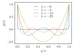
Figure 1: Solutions $g(u)=\sum_{n=1}^{n_{\rm max}}g_{n}\cos(2nu)$ deduced from the numerical solution of Eqs. (50) with $n_{\rm max}=400$ and $\theta=0.5$, and corresponding to the largest eigenvalues: $\lambda=-\theta=-0.5$ (solid line) and $\lambda\simeq-3.00/-12.00/-25.00$ (dashed and dotted lines). The functions are normalized by the condition $g(0)=1$.

If we set $K\equiv K_{\Lambda}=0$ in the flow equation (28) the cusp in $\delta_{ii,k}(u)$ arises for $k>0$.Dupuis and Daviet (2020) This finite-scale singularity is not accounted for in the linear analysis. Indeed, if we set $K=0$ in (46) and (47), we find that the function $g(u)e^{\lambda t}$ goes smoothly to zero and the fixed point $\delta^{*}(u)$ is recovered only for $k=0$. Thus it seems that the boundary layer induced by a nonzero $K_{k}$ is a necessary condition for the linear analysis to be valid.

III.2 Escape from the BG fixed point

III.2.1 Chaotic behavior and overlap length

When $\epsilon=0$ the two copies are identical, $\delta_{12,k}(u)=\delta_{ii,k}(u)$, and $\delta_{12,k}(u)$ approaches $\delta^{*}(u)$ when $k\to 0$. For small but nonzero $\epsilon$, implying $\delta_{12,\Lambda}(u)\neq\delta_{ii,\Lambda}(u)$, $\delta_{k,12}(u)$ is first attracted to the BG fixed-point solution $\delta^{*}(u)$ but is eventually suppressed as shown in Fig. 2:

$$\lim_{k\to 0}\delta_{12,k}(u)=0.$$ (54)

Linearizing the equation $\partial_{t}\delta_{12,k}$, we find

$$\delta_{12,k}(u)\sim k^{-3+\pi^{2}/3}\cos(2u)\quad\mbox{for}\quad k\to 0$$ (55)

(higher-order harmonics decay faster), which gives $G_{d,12,k=0}(q,0)\sim|q|^{-4+\pi^{2}/3}$, so that

$$C_{12}(X)\sim\frac{1}{|x|^{-3+\pi^{2}/3}}$$ (56)

decays with the exponent $\pi^{2}/3-3\simeq 0.2899$. We conclude that the BG phase exhibits chaos.

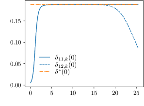
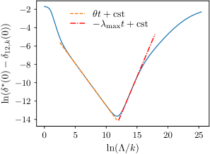
Figure 2: (top) $\delta_{11,k}(0)=\delta_{22,k}(0)$ and $\delta_{12,k}(0)$ vs $\ln(\Lambda/k)=-t$ as obtained from the numerical solution of the flow equations with $n_{\rm max}=800$ and $\epsilon\simeq 3\times 10^{-8}$. When $\epsilon\neq 0$, $\delta_{12,k}(0)$ first approaches the BG fixed-point value $\delta^{*}(0)$ but is eventually suppressed, $\lim_{k\to 0}\delta_{12,k}(0)=0$, thus showing that the two copies become statistically uncorrelated at long distances. (bottom) The ln-ln plot shows that the approach of $\delta_{12,k}(0)$ to its fixed point value $\delta^{*}(0)$ is controlled by the exponent $-\theta$ and the escape by $\lambda_{\rm max}\simeq 1.6$. (These figures are obtained for $K=0.1$, other figures use $K=0.4$.)

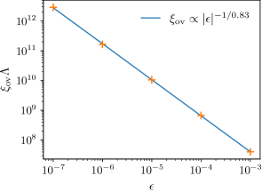
Figure 3: $\xi_{\rm ov}$ vs $\epsilon$ in a log-log plot as obtained from the criterion $F_{k=1/\xi_{\rm ov}}=0.1$. The blue line shows a linear fit corresponding to the power-law behavior (57) with $\alpha\simeq 0.83$.

We can define a characteristic (overlap) length $\xi_{\rm ov}\equiv\xi_{\rm ov}(\epsilon)$ associated with the instability of the BG fixed point when $\epsilon\neq 0$ and signaling the loss of statistical correlations between the two copies at large length scales. We use the criterion $F_{k=1/\xi_{\rm ov}}=\gamma$ where $\gamma\ll 1$ is an arbitrary number and $F_{k}$ is defined by (27). $\xi_{\rm ov}$ diverges for $\epsilon\to 0$ as a power law (Fig. 3),

$$\xi_{\rm ov}\propto|\epsilon|^{-1/\alpha},$$ (57)

where $\alpha$ is the chaos exponent. If we plot $F_{k}$ as a function of $k\xi_{\rm ov}$ for various values of $\epsilon$, we observe a data collapse thus showing that $F_{k}$ satisfies the one-parameter scaling form

$$F_{k}={\cal F}(k\xi_{\rm ov}),$$ (58)

where ${\cal F}(x)$ is a universal scaling function, as expected for a scale-invariant fixed point with a single relevant direction (Fig. 4).

On can also obtain the chaos exponent directly from the flow equations. For $\epsilon\to 0$, when $\delta_{12,k}(0)$ is near its fixed point value $\delta^{*}(0)$, one has

$$\delta_{12,k}(0)\simeq\delta^{*}(0)+Ae^{\theta t}+Be^{-\lambda_{\rm max}t},$$ (59)

as shown in Fig. 2. The leading irrelevant eigenvalue $-\theta$, as discussed in Sec. III.1.2, controls the approach to the BG fixed point. The relevant eigenvalue $\lambda_{\rm max}$ controls the departure from the fixed point at very long RG time $|t|$. $\lambda_{\rm max}$ also determines the divergence of the overlap length when $\epsilon\to 0$,

$$\xi_{\rm ov}\sim|\delta_{12,\Lambda}(0)-\delta_{ii,\Lambda}(0)|^{1/\lambda_{\rm max}}\sim|\epsilon|^{-2/\lambda_{\rm max}},$$ (60)

so that $\alpha=\lambda_{\rm max}/2$. The estimate of the chaos exponent obtained from (59) is in very good agreement with the calculation of $\xi_{\rm ov}$ using the criterion $F_{k=1/\xi_{\rm ov}}=\gamma$. The results are shown in Table 1 for various values of $n_{\rm max}$.

Table 1: Chaos exponent $\alpha$ vs number $n_{\rm max}$ of harmonics used in the numerics obtained from $\xi_{\rm ov}$, $\delta_{12,k}(0)-\delta^{*}(0)$ or the linear analysis [Eqs. (68)].

$n_{\rm max}$	100	200	300	400	500	600	1000	10000	20000	30000	40000	50000	100000
from $\xi_{\rm ov}$	0.803	0.816	0.826	0.831	0.832
from $\delta_{12,k}(0)-\delta^{*}(0)$	0.800	0.811	0.817	0.820	0.823
from linear analysis	0.717	0.748	0.764	0.773	0.781	0.786	0.800	0.847	0.857	0.862	0.865	0.868	0.876

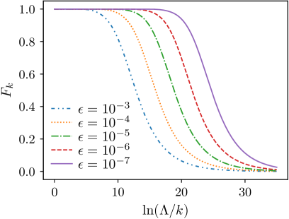
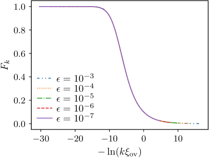
Figure 4: (top) $F_{k}$ vs $k$ for various values of $\epsilon$. Statistical correlations between the two copies are lost when $1/k$ is larger than the overlap $\xi_{\rm ov}$ length defined by $F_{k=1/\xi_{\rm ov}}=0.1$. (bottom) $F_{k}$ vs $k\xi_{\rm ov}$ showing the data collapse expected from the scaling form (58).

III.2.2 Chaos boundary layer

The boundary layer analysis of Sec. III.1.1 can be generalized to the case where $\epsilon\neq 0$. Since the flow equation of $\delta_{ii,k}(u)$ and $K_{k}$ are independent of $\epsilon$, the intracopy disorder correlator $\delta_{ii,k}(u)$ is still given by (34) when $|u|,K_{k}\ll 1$. The equation for $\delta_{12,k}(u)$ can be written as

$$\partial_{t}\delta_{12,k}(u)={} -3\delta_{12,k}(u)-l_{1}\left(K_{k}+\frac{\pi\bar{l}_{2}}{l_{1}}\hat{K}_{k}\right)\delta^{\prime\prime}_{12,k}(u)$$

$$+\pi\bar{l}_{2}\{\delta_{12,k}^{\prime\prime}(u)[\delta_{12,k}(u)-\delta_{12,k}(0)]+\delta^{\prime}_{12,k}(u)^{2}\},$$ (61)

where

$$\hat{K}_{k}=\delta_{ii,k}(0)-\delta_{k,12}(0).$$ (62)

We assume that the system is near the BG fixed point, so that both $K_{k},\hat{K}_{k}$ and their derivatives $\partial_{t}K_{k},\partial_{t}\hat{K}_{k}$ are small.not (d) Near $u=0$, but for an arbitrary ratio $u/K_{{\rm tot},k}$, the solution of (61,62) can be written in the form

$$\delta_{12,k}(u)=\delta_{12,k}(0)+K_{{\rm tot},k}f\left(\frac{u}{K_{{\rm tot},k}}\right),$$ (63)

where

$$K_{{\rm tot},k}=K_{k}+\frac{\pi\bar{l}_{2}}{l_{1}}\hat{K}_{k}.$$ (64)

Using the fact that $K_{{\rm tot},k}$ and $\partial_{t}K_{{\rm tot},k}$ are small, Eq. (61) implies that $f(x)$ satisfies (36) and is therefore given by (37) with $f^{\prime\prime}(0)=-\pi/4l_{1}\bar{l}_{2}$. This is expected since when $\epsilon=0$, one has $K_{{\rm tot},k}=K_{k}$ and $\delta_{12,k}(u)=\delta_{ii,k}(u)$ is given by (34). Similarly to (41) we find

$$\delta_{12,k}(0)=\delta^{*}(0)-\frac{l_{1}}{\pi\bar{l}_{2}}K_{{\rm tot},k}.$$ (65)

When $\delta_{12,k}(u)$ approaches the fixed point, i.e., when $K_{{\rm tot},k}\simeq K_{k}$, the decreasing width of the boundary layer is controlled by quantum fluctuations as discussed in Sec. III.1.1 ($\delta_{12,k}(u)\simeq\delta_{ii,k}(u)$ in that case). At latter RG times $|t|$, when $K_{{\rm tot},k}\simeq(\pi\bar{l}_{2}/l_{1})\hat{K}_{k}$, the width of the boundary layer increases as a result of the loss of statistical correlations between the two copies due to the chaotic behavior of the system. Equations (63,65) are in very good agreement with the numerical solution of the flow equations as shown in Fig. 5.

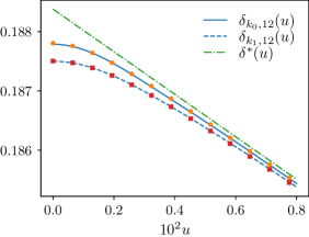
Figure 5: $\delta_{12,k}(u)$ near $u=0$ as obtained from the numerical solution of the flow equations (lines) and the analytic expression (63) (symbols). $\delta_{12,k_{0}=\Lambda e^{-4.5}}$ shows the QBL that forms during the approach to the BG fixed point whereas $\delta_{12,k_{1}=\Lambda e^{-18.5}}$ shows the CBL due to the escape of the fixed point. When using expression (63), the value of $K_{{\rm tot},k}$ is obtained from the numerical solution of the flow equations.

III.2.3 Linear analysis

We now consider a linear analysis of the perturbations about the BG fixed point in the case $\epsilon\neq 0$. Writing

$$\begin{split}\delta_{ii,k}(u)&=\delta^{*}(u)+g_{ii}(u)e^{-\lambda t},\\ \delta_{12,k}(u)&=\delta^{*}(u)+g_{12}(u)e^{-\lambda t},\\ K_{k}&=K^{*}+Ke^{-\lambda t}\end{split}$$ (66)

(note that $\hat{K}_{k}$, introduced in the preceding section, is not an independent variable), we obtain

$$\lambda g_{12}(u)={} 3g_{12}(u)+Kl_{1}\delta^{*}{}^{\prime\prime}(u)-\pi\bar{l}_{2}\{g^{\prime\prime}_{12}(u)[\delta^{*}(u)-\delta^{*}(0)]$$

$$+\delta^{*}{}^{\prime\prime}(u)g_{12}(u)+2\delta^{*}{}^{\prime}(u)g_{12}^{\prime}(u)\}$$ (67)

to first order in $g_{12}$ while $g_{ii}$ and $K$ satisfy (46,47). Expanding both $g_{ij}(u)$ and $\delta^{*}(u)$ in circular harmonics yields the linear system

$$\begin{split}\lambda g_{ii,n}&=\sum_{n^{\prime}=1}^{\infty}A_{n,n^{\prime}}g_{ii,n^{\prime}}-\frac{2l_{1}}{\pi\bar{l}_{2}}K,\\ \lambda g_{12,n}&=\sum_{n^{\prime}=1}^{\infty}B_{n,n^{\prime}}g_{12,n^{\prime}}-\frac{2l_{1}}{\pi\bar{l}_{2}}K,\\ \lambda K&=-\theta K,\end{split}$$ (68)

where $A_{n,n^{\prime}}$ is defined in (51) and

$$B_{n,n^{\prime}}=A_{n,n^{\prime}}+2.$$ (69)

Using

$$\sum_{n^{\prime}=1}^{\infty}B_{n,n^{\prime}}=2,$$ (70)

which follows from (52), we see that $K=0$ and $g_{12,n}={\rm const}$, i.e.,

$$g_{12}(u)=\pi\mbox{\tencyr SH}(u)-1,$$ (71)

is solution with eigenvalue $\lambda=2$ and satisfies $\int_{0}^{\pi}du\,g_{12}(u)=0$. It qualitatively reproduces the result obtained from the boundary layer analysis in Sec. III.2.2 although the latter gives a Kronecker comb and not a Dirac comb (see the discussion in Sec. III.1.2). We do not expect the difference between the Kronecker and Dirac combs to bear a particular physical meaning. In both cases the singular function $g_{12}(u)$ originates from the boundary layer near $u=p\pi$, be it a QBL or a CBL [Eq. (63)]. Similarly we find that $g_{12}(u)$ defined by (71), together with

$$K=\frac{\pi\bar{l}_{2}}{l_{1}}(\theta+2),$$ (72)

is solution with eigenvalue $\lambda=-\theta$.

Let us now look for the other eigenfunctions, with $\lambda\neq 2,-\theta$ and therefore $K=0$, in the form

$$g(u)=\pi\mbox{\tencyr SH}(u)-1+h(u),$$ (73)

where $h(u)$ is assumed to be free of Dirac peaks but its derivative may be discontinuous at $u=p\pi$. From the equations satisfied by $g(u)$ and $\pi\mbox{\tencyr SH}(u)-1$, we easily obtained

$$(\lambda-2)[\pi\mbox{\tencyr SH}(u)-1]+\lambda h(u)=3h(u)-\pi\bar{l}_{2}\{\delta^{*}{}^{\prime\prime}(u)h(u)\\ +h^{\prime\prime}(u)[\delta^{*}(u)-\delta^{*}(0)]+2\delta^{*}{}^{\prime}(u)h^{\prime}(u)\}.$$ (74)

Collecting all terms involving Dirac peaks,not (e) we obtain

$$(\lambda-2)\pi\mbox{\tencyr SH}(u) =\pi\mbox{\tencyr SH}(u)h(u)$$

$$=\pi\mbox{\tencyr SH}(u)h(0).$$ (75)

This equation is satisfied if

$$h(0)=\lambda-2.$$ (76)

The terms free of Dirac peaks lead to the equation

$$0=(4-2\lambda)(h-1)+u(\pi-u)h^{\prime\prime}+2(\pi-2u)h^{\prime}$$ (77)

for $u\in[0,\pi]$. Setting $h=1+f$ and introducing $x=u/\pi$, we finally obtain

$$0=(4-2\lambda)f+x(1-x)f^{\prime\prime}+2(1-2x)f^{\prime},$$ (78)

where the function $f(x)$ must satisfy

$$\int_{0}^{1}dx\,f(x)=-1.$$ (79)

Equation (78) was studied by DLD.Duemmer and Le Doussal (2007) The solutions that are symmetric about $x=1/2$ in the interval $[0,1]$ (this condition follows from $h(u)$ being even and $\pi$ periodic) can be expressed in terms of hypergeometric functions. The condition (79) of integrability selects a discrete set of values of $\lambda$, for which the hypergeometric function becomes a polynomial function of finite order,

$$f(x)=\sum_{m=0}^{m_{0}}c_{m}x^{m}.$$ (80)

For $f(x)$ to be solution of (78), we must require

$$c_{m+1}=c_{m}\frac{m(m+3)-4+2\lambda}{(m+1)(m+2)},$$ (81)

whereas $c_{0}$ is determined from (79). Imposing $c_{m_{0}+1}=0$ then gives

$$\lambda=2-\frac{m_{0}(m_{0}+3)}{2}.$$ (82)

For $m_{0}=0$ we obtain $\lambda=2$ and $f(x)=-1$, i.e., $h(u)=0$, which reproduces the solution (71). The choice $m_{0}=1$, and more generally $m_{0}$ odd, must be discarded since the corresponding solutions do not satisfy $f(0)=f(1)$. For $m_{0}=2$, one finds $\lambda=-3$ and

$$f(x)=-6(1-5x+5x^{2}).$$ (83)

The condition (76), $\lambda=2+h(0)=3+f(0)$, is satisfied. The next solution ($m_{0}=4$) corresponds to $\lambda=-12$ and

$$f(x)=-15(1-14x+56x^{2}-84x^{3}+42x^{4}),$$ (84)

and satisfies (76). All other solutions can be obtained similarly and are associated with eigenvalues that are more and more irrelevant as $m_{0}$ increases. The negative eigenvalue spectrum $\{-3,-12,-25,-42,-63,-88,\cdots\}$ is the same as that obtained numerically for the approach to the BG fixed point.

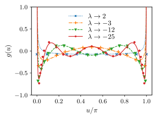
Figure 6: Functions $g(u)$, corresponding to the four largest eigenvalues, obtained from the numerical solution of (68) with $n_{\rm max}=1000$ (symbols). Away from the points $u=0$ and $u=\pi$, these functions are well approximated by the functions $f(u)$ solutions of (78) associated with the eigenvalues $2/-3/-12/-25$, with an appropriate normalization (lines).

In Fig. 6 we show the solution $g(u)$ obtained from a numerical solution of (68) with a finite number $n_{\rm max}$ of circular harmonics. We find that there is a single positive eigenvalue (in agreement with the analytic results), associated with a function $g(u)$ which, as $n_{\rm max}$ increases, is more strongly peaked near $u=p\pi$, with however a nonzero value away from these two points to ensure that $\int_{0}^{\pi}du\,g(u)=0$. This behavior is in qualitative agreement with (71). The functions $g(u)$ associated with negative eigenvalues are also strongly peaked near $u=0$ and $u=\pi$, and their behavior away from these two points is well approximated by the function $f(u)=g(u)-\pi\mbox{\tencyr SH}(u)$ found analytically above (Fig. 6). The convergence with $n_{\rm max}$ of the eigenvalues to the spectrum (82) is however extremely slow. Even for a relatively large value $n_{\rm max}=100\,000$ we find that $\lambda_{\rm max}\simeq 1.75$ is still far from its expected converged value $\lambda_{\rm max}=2$. Our results agree with a logarithmic convergence,

$$\lambda_{\rm max}(n_{\rm max})\simeq a-\frac{b}{c+\ln(n_{\rm max})}$$ (85)

with $a\simeq 2.03$, $b\simeq 3.70$ and $c\simeq 1.77$, as shown in Fig. 7.

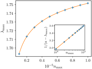
Figure 7: Largest eigenvalue $\lambda_{\rm max}$ vs $n_{\rm max}$ obtained from the numerical solution of (68). The continuous (orange) line shows the logarithmic convergence (85) of $\lambda_{\rm max}$ with $n_{\rm max}$.

The various values of the chaos exponent obtained numerically from either $\xi_{\rm ov}$, $\delta_{12,k}(0)-\delta^{*}(0)$ or the linear analysis, are shown in Table 1. Our analytic result $\lambda_{\rm max}=2$ implies a chaos exponent $\alpha=\lambda_{\rm max}/2=1$.

The slow convergence of $\lambda_{\rm max}$ with $n_{\rm max}$ implies that it is necessary to probe the system at very long length scales to observe the value $\alpha=1$ of the chaos exponent. Any finite length $L$ indeed introduces an effective upper cutoff $n_{\rm max}\sim 1/L$ on the number of circular harmonics in the Fourier series expansion of the function $\delta_{12,k}(u)$. In particular this means that the critical behavior $\xi_{\rm ov}\sim|\epsilon|^{-1/\alpha}$ will be observed only if $\xi_{\rm ov}$ is sufficiently large (i.e., $|\epsilon|$ sufficiently small). Thus, to determine the chaos exponent from the numerical solution of the flow equations, one would need both a very small value of $\epsilon$ and an extremely large $n_{\rm max}$, which cannot be realized in practice.

III.2.4 Comparison with Duemmer and Le Doussal’s work

Equations (28,29) and (67) are identical to those obtained by DLD in their study of periodic elastic manifolds pinned by disorder (with the temperature playing the role of the Luttinger parameter).Duemmer and Le Doussal (2007) But our analysis of the linearized equation (67) differs in a crucial way: DLD use $\delta^{*}{}^{\prime\prime}(u)=1/\pi\bar{l}_{2}$ which contradicts (49) and is not correct since it violates the condition $\int_{0}^{\pi}du\,\delta^{*}{}^{\prime\prime}(u)=0$. As a result, they obtain equation (78) for the function $g$ instead of $f=g-\pi\mbox{\tencyr SH}$.not (f) Since none of the solutions of this equation have a vanishing integral over the interval $[0,1]$ they conclude that the linear analysis of perturbations about the fixed point fails.

To circumvent this difficulty DLD consider a two-dimensional system where the temperature is marginal, $\theta=0$, and therefore does not flow under RG. When $\epsilon=0$ one obtains a line of fixed points indexed by $T>0$. The function $\delta^{*}(u)$ is analytic and exhibit a thermal boundary layer (TBL) of width $T$ instead of the cusp, which makes the linear analysis about the fixed point free of the difficulties that arise when the temperature flows toward zero. DLD find that outside the TBL (i.e. for $|u|\gtrsim T$) the eigenfunction $g(u)$ corresponding to the largest eigenvalue $\lambda$ must be chosen among the solutions $f(u)$ of (78), whereasnot (g)

$$g(u)=\frac{1}{6T}\frac{\lambda-2}{\left[1+\left(\frac{u}{2T}\right)^{2}\right]}$$ (86)

for $|u|\lesssim T$. The eigenvalue

$$\lambda\simeq 2-\frac{3}{\ln(1/T)}$$ (87)

converges logarithmically toward 2 when $T\to 0$. We conclude that the $T\to 0$ limit of DLD’s results in the marginal case $\theta=0$ agree with the conclusions of Sec. III.2.3 obtained in the case where the temperature $T$ (i.e., the Luttinger parameter in our notations) flows to zero ($\theta>0$). Our results show that the $T\to 0$ limit of the function $g(u)$ inside the TBL [Eq. (86)] is given by the singular function $\mbox{\tencyr SH}(u)$. The temperature dependence of the eigenvalue in (87) is similar to the dependence of $\lambda$ with respect to $n_{\rm max}$ in (85). These logarithmic corrections are due to the finite length scale introduced by the finite temperature in the marginal case ($\theta=0$) or the finite number of circular harmonics in our study ($\theta>0$).

DLD also consider a system with dimensionality larger than two where the temperature is irrelevant ($\theta>0$). In that case they find that the escape from the fixed point, i.e., the growth of $\delta_{12,k}(u)-\delta_{ii,k}(u)$, occurs with eigenvalue $\lambda=2$ if $u$ is outside the CBL and $2+\theta$ if $u$ is inside the CBL, which gives the chaos exponent $\alpha=2/(2+\theta)$. This latter result disagrees with our conclusions.

IV Quantum chaos

In this section we consider two copies of the system subjected to the same disorder potential but with different Luttinger parameters,

$$\begin{split}K_{1}&=K+\epsilon,\\ K_{2}&=K-\epsilon.\end{split}$$ (88)

The replicated action is then given by

$$S[\{\varphi_{ia}\}]=\sum_{i,a}\int_{x,\tau}\frac{v}{2\pi K_{i}}\left\{(\partial_{x}\varphi_{ia})^{2}+\frac{({\partial_{\tau}}\varphi_{ia})^{2}}{v^{2}}\right\}\\ -\sum_{a,b,i,j}{\cal D}\int_{x,\tau,\tau^{\prime}}\cos[2\varphi_{ia}(x,\tau)-2\varphi_{jb}(x,\tau^{\prime})].$$ (89)

In order to implement the FRG, we choose a cutoff function which depends on the copy index,

$$R_{i,k}(q,i\omega)=Z_{ix}\left(q^{2}+\frac{\omega^{2}}{v_{i,k}^{2}}\right)r\left(\frac{q^{2}+\omega^{2}/v_{i,k}^{2}}{k^{2}}\right),$$ (90)

where $Z_{ix}=v/\pi K_{i}$ and $v_{i,k}$ is the renormalized velocity of the $i$th copy.

The ansatz for the effective action $\Gamma_{k}[\{\phi_{ia}\}]$ is given by (22) with $Z_{x}$ and $v_{k}$ replaced by $Z_{ix}$ and $v_{i,k}$. The flow equations for $K_{i,k}$, $v_{i,k}$ and

$$\delta_{ij,k}(u)=-\frac{K_{i}K_{j}}{v^{2}k^{3}}V^{\prime\prime}_{ij,k}(u)$$ (91)

are given by

$$\begin{split}\partial_{t}K_{i,k}&=\theta_{i,k}K_{i,k},\qquad\partial_{t}(K_{i,k}/v_{i,k})=0,\\ \theta_{i,k}&=\frac{\pi}{2}\delta^{\prime\prime}_{ii,k}(0)\bar{m}_{\tau}.\end{split}$$ (92)

and

$$\partial_{t}\delta_{ii,k}(u)={} -3\delta_{ii,k}(u)-l_{1}K_{i,k}\delta^{\prime\prime}_{ii,k}(u)$$

$$+\pi\bar{l}_{2}\{\delta_{ii,k}^{\prime\prime}(u)[\delta_{ii,k}(u)-\delta_{ii,k}(0)]+\delta^{\prime}_{ii,k}(u)^{2}\},$$ (93)

$$\partial_{t}\delta_{12,k}(u)={} -3\delta_{12,k}(u)-l_{1}\frac{K_{1,k}+K_{2,k}}{2}\delta^{\prime\prime}_{12,k}(u)$$

$$+\pi\bar{l}_{2}\{\delta_{12,k}^{\prime\prime}(u)[\delta_{12,k}(u)-\delta_{12,k}(0)]+\delta^{\prime}_{12,k}(u)^{2}\}$$

$$-\pi\bar{l}_{2}\hat{K}_{k}\delta^{\prime\prime}_{12}(u),$$ (94)

where

$$\hat{K}_{k}=\frac{\delta_{11,k}(0)+\delta_{22,k}(0)}{2}-\delta_{12,k}(0).$$ (95)

These equations are similar to those discussed in Secs. II and III. Since $\hat{K}_{\Lambda}={\cal O}(\epsilon^{2})$, all conclusions reached in Sec. III remain valid as can be explicitly verified by solving numerically the flow equations. The chaotic behavior now originates in the difference in the quantum fluctuations of the two copies of the system. Although they are suppressed in the long-distance limit, $K_{i,k}\to 0$ for $k\to 0$, they select different ground states in the two copies. This “quantum” chaos is analog to the “temperature” chaos in classical disordered system, as shown by the analogy between Eqs. (93) and (94) and the equations derived in Ref. Le Doussal, 2006.

V Conclusion

We have investigated the chaotic behavior of the BG phase of a one-dimensional disordered Bose fluid. By solving numerically the nonperturbative FRG equations, we find that two copies of the system with slightly different disorder configurations become statistically uncorrelated at large distances. The chaos exponent $\alpha$ can be obtained from the overlap length $\xi_{\rm ov}\sim|\epsilon|^{-1/\alpha}$ or the growth of $\delta_{12,k}(0)-\delta^{*}(0)\sim e^{-2\alpha t}$ at long RG time $|t|$, but the convergence with the number $n_{\rm max}$ of circular harmonics used for the disorder correlators $\delta_{ij,k}(u)$ turns out to be logarithmic and therefore extremely slow. From the linear analysis of perturbations about the BG fixed point, we are however able to show analytically that $\alpha=1$.

Although the chaos exponent is related to the relevant RG eigenvalue $\lambda_{\rm max}=2\alpha$ of the linearized flow near the BG fixed point, as for a standard critical point, the peculiar nature of the fixed point makes the situation somewhat unusual. The fixed-point disorder correlator $\delta^{*}(u)$ exhibits cusps at $u=p\pi$ and $\delta_{12,k}(u)$ approaches and departs from its nonanalytic fixed-point form via a QBL and a CBL, respectively. This has strong consequences for the linear analysis of the perturbations about the fixed point. The eigenfunctions $g_{12,k}(u)\equiv\delta_{12,k}(u)-\delta^{*}(u)=\pi\mbox{\tencyr SH}(u)+f(u)$, solutions of the linearized flow equations, are singular at $u=p\pi$ ($f(u)$ is a regular function). Although this could call into question the linear analysis, the agreement with the results obtained from the numerical analysis of the flow equations, where the function $\delta_{12,k}(u)$ remains analytic at all scales $k\geq 0$, strongly supports its validity, even if this agreement is obtained for a finite number $n_{\rm max}$ of circular harmonics for which the chaos exponent significantly differs from its converged value.

The chaotic behavior of the BG phase can also be induced by a modification of quantum fluctuations due to a slight variation of the Luttinger parameter.

Finally we note that all these conclusions also apply to the Mott-glass phase of a disordered Bose fluid induced by long-range interactions.Daviet and Dupuis (2020)