Decays of Higgs Bosons in the Standard Model and Beyond

Abstract

We make an updated review and a systematic and comprehensive analysis of the decays of Higgs bosons in the Standard Model (SM) and its three well-defined prototype extensions such as the complex singlet extension of the SM (cxSM), the four types of two Higgs-doublet models (2HDMs) without tree-level Higgs-mediated flavor-changing neutral current (FCNC) and the minimal supersymmetric extension of the SM (MSSM). We summarize the theoretical predictions for the decay widths of the SM Higgs boson and those of Higgs bosons appearing in its extensions taking account of all possible decay modes. We incorporate them to study and analyze decay patterns of CP-even, CP-odd, and CP-mixed neutral Higgs bosons and charged ones. We put special focus on the properties of a neutral Higgs boson with mass about 125 GeV discovered at the LHC and present constraints obtained from precision analysis of it. This review is intended to be self-contained and consolidated by coherently integrating relevant physics information for studying decays of Higgs bosons in the SM and beyond.

1 Introduction

Since the discovery of a resonance with a mass of approximately 125 GeV at the Large Hadron Collider (LHC) in 2012 [1, 2], the substantial subsequent studies of its properties have been carried out with the data set collected during the LHC Run 1 period from 2009 to 2012 and the LHC Run 2 period from 2015 to 2018. They have firmly confirmed the compatibility of the resonance with the spin-zero and parity-even SM Higgs boson which appears in the spontaneously broken gauge theory where the electroweak interactions are governed by the SU(2)${}_{L}\times{\rm U(1)}_{Y}$ gauge symmetry group [3, 4, 5]. At the present time we are on a watershed peak for exploring a new territory of particle physics through the Higgs landscape.

The total and differential rate measurements of all the possible production and decay channels of the resonance state so far are consistent with those predicted in the SM within experimental and theoretical uncertainties [7, 8]. The mass of the Higgs boson has been measured at the per-mille precision level, mainly through the high-resolution decay modes with four-lepton and di-photon final states [9, 10]. Furthermore, the couplings of the Higgs boson to the gauge bosons and the charged fermions of the third generation [11, 12, 13, 14, 15] and, recently, to the muons [16, 17] were established independently and unambiguously. Based on the observational facts, we call the discovered resonance particle as the SM-like Higgs boson wherever appropriate in the following.

Nevertheless, the couplings of the SM-like Higgs boson to the electrons and lighter quarks of the first and second generations and its cubic and quartic self-couplings defining the profile of the Higgs potential are yet to be established and measured independently. Furthermore, more complex Higgs sectors associated with additional states have not been ruled out. Therefore, it is not yet firmly established whether the SM-like Higgs boson is indeed the only elementary scalar state as in the SM, whether there exist additional elementary scalar particles, or even whether it is a composite particle with internal structure or not.

Conceptually, the SM with the Higgs boson could be weakly interacting well above the weak scale of $v=246$ GeV without violating unitarity and so with no need for new physics. However the Higgs boson mass is influenced subtly by the presence of heavy particles and it receives quantum corrections destabilizing the weak scale and requiring a delicate fine-tuning of apparently unrelated parameters. This so-called naturalness or hierarchy problem [18, 19, 20] has been the key argument for expecting new physics to be revealed at the TeV scale. To mention just a few, new theoretical frameworks based on a fermion-boson symmetry called supersymmetry [21, 22, 23], a collective symmetry between the SM particles and heavier partners as in Little Higgs theories [24, 25, 26] or an effective reduction of the Planck scale to the TeV scale as in extra-dimension models [27, 28, 29, 30] have been proposed and intensively investigated.

In addition to alleviating the hierarchy problem, new scenarios involving extensions of the Higgs sector generically have been proposed and investigated to account for the dark matter (DM) abundance [31, 32], the matter-antimatter asymmetry of the Universe with new sources of the charge-parity (CP) symmetry breakdown [33, 34, 35], the tiny but non-vanishing neutrino masses [36], inflation [37], etc. Such models with additional scalars can provide us with solid platforms for exploring new Higgs boson signals concretely and comprehensively since, in each scenario, Higgs bosons exhibit their own distinctive features in their couplings to gauge bosons, fermions and those among themselves.

After the successful completion of Run 1 and Run 2, the LHC is presently in the second long shut down period while undergoing important upgrades for its high luminosity phase. Much larger data sets are to be collected during the Run 3 period and, ultimately, during the operation period of the high-luminosity LHC (HL-LHC) and they will enable us to explore new physics beyond the SM (BSM) by performing more challenging as well as more precise measurements. In light of such promising experimental prospects at the LHC and at other future high-energy and high-precision experiments [38, 39] it is quite timely and worthwhile to perform a systematic and comprehensive review and analysis of the decays of Higgs bosons including the theoretical calculations known up to now, not only in the SM but also in various BSM scenarios with unique features in their extended Higgs sectors.

Certainly it is formidable to review all theoretical and experimental aspects of Higgs sectors in all BSM models proposed so far in a single report with limited space. Unavoidably, we restrict ourselves in this review to the SM and the three well-defined prototype BSM models with extended Higgs sectors possessing their own characteristic features and broad implications. Specifically, in addition to the SM, we consider the following representative examples: $(i)$ the complex singlet extension of the SM (cxSM) [40, 41, 42, 43, 44, 45, 46, 47, 48], $(ii)$ the four types of two Higgs doublet models (2HDMs) [49, 50, 51, 52, 53, 54, 55, 56, 57, 58, 59] with natural flavor conservation at the tree level and the so-called $\rho$ parameter close to unity abiding by the stringent experimental constraint on it, and $(iii)$ the minimal supersymmetric extension of the SM (MSSM) [60, 61, 62, 63, 64, 65, 66, 67, 68, 69]. For Higgs sectors in BSM models beyond cxSM, 2HDMs and MSSM, see, for example, Refs. [70, 71, 72, 73, 74, 75].

Several related previous reviews on Higgs physics in the SM and the MSSM can be found in Refs. [76, 77, 58, 78, 79, 80, 81, 82, 83, 84, 85, 86, 87, 88]. A few tailor-made sophisticated computational packages have been developed for the mass spectra and decay widths of neutral and charged Higgs bosons in the SM and the MSSM with real parameters [89, 90, 91] and with explicit CP violation [92, 93, 94, 95, 96]. This review updates the previous works substantially by including two popular BSM models in addition to the MSSM and also by allowing for complex parameters leading to CP-violating phenomena [80, 97]. We perform a systematic and comprehensive analysis for the decays of neutral and charged Higgs bosons in those three prototype BSM models as well as in the SM. We take account of all possible decay modes of these models including those into non-SM particles among which some are invisible [98, 99] and/or exotic [100]. We anticipate more complete reviews on the Higgs sectors of many other BSM scenarios to come out timely in step with more advanced experimental developments.

In this review, we try to contain all the relevant information needed to implement the up-to-date theoretical calculations of Higgs decays. We aim to make it be of pedagogical and practical use especially for incorporating corrections beyond the leading order (LO). We elaborate on how the partial decay widths of neutral and charged Higgs bosons are calculated at LO and how we treat QCD and electroweak (ELW) corrections in each decay mode. We intend to make this review stand-alone, self-contained, and consolidated by integrating relevant physics information for Higgs decays coherently. Incidentally, we try to make it be as model-independent and analytic as possible in order for our approach to be useful and easily applicable in studying Higgs decays even in the BSM models not explicitly mentioned in this review.

This review is organized as follows. Section 2 is devoted to reviewing the Higgs sectors of the SM and three extended scenarios - cxSM, 2HDMs and MSSM - without imposing any constraints on the model parameters. We work out the analytic structure of the Higgs potential and mixing. Also worked out are the Higgs interactions with gauge bosons, the SM fermions, and new scalars and fermions as well as the Higgs-boson self interactions. We review and update the decays of neutral Higgs bosons in Section 3 and those of charged Higgs bosons in Section 4. We provide explicit analytical expressions of the individual partial decay widths as precisely as possible by including the state-of-the-art theoretical calculations. In Section 5, we present the constraints on the couplings of the SM-like Higgs boson weighing about 125 GeV obtained from global fits to the LHC precision Higgs data. Conclusions are made in Section 6. To make this review self-contained, various supplemental materials are provided in six appendices. Appendix A includes a summary of the SM parameters used for the numerical estimates of the Higgs decay widths and a description of the running of the strong coupling constant and heavy quark masses. In Appendix B, the supersymmetric contributions to the loop-induced couplings of the Higgs boson to two gluons, two photons and $Z\gamma$ are presented and Appendix C is devoted to the presentation of the QCD corrections to the partial width of the Higgs-boson decay to two photons. In Appendix D, we present expressions for the most general 2HDM potential parameters in terms of the masses of charged and neutral Higgs bosons and the elements of the orthogonal matrix describing the mixing among neutral Higgs bosons and, in Appendix E, we apply them for deriving cubic Higgs-boson self-couplings. Finally, Appendix F is added as a guide to numerical packages for calculating precise SM and full BSM-dependent ELW corrections.

2 Standard Model and Beyond

In this section, we derive and describe the basic form of Higgs boson masses and mixing as well as their interactions in the SM, cxSM, 2HDMs and MSSM. The derived analytical results are utilized comprehensively in the sequential sections for the detailed review of the decays of neutral and charged Higgs bosons and also for the model-independent precision study of the SM-like neutral Higgs boson which has been extensively probed at the LHC since its discovery in 2012.

We note that there are codes such as FeynRules [101, 102, 103], Sarah [104, 105, 106, 107], and LanHEP [108, 109, 110, 111, 112, 113, 114] for the automatic generation of all the Feynman rules in the BSM models as well as in the SM. Rather than simply using these codes, we start by presenting interaction Lagrangians in order for the readers to work out independently the analytic structure and parametric dependence of the partial decay widths of neutral and charged Higgs bosons and to more deeply understand the theoretical and phenomenological aspects of Higgs physics in the SM and beyond.

2.1 Standard Model

The self-interactions of the SM Higgs boson and its interactions with the massive vector bosons are derived from the Higgs Lagrangian:

$${\cal L}_{\rm Higgs}=\left(D^{\mu}\Phi\right)^{\dagger}\left(D_{\mu}\Phi\right)\ -\ V_{\rm SM}(\Phi)\,,$$ (1)

where $\Phi$ denotes a complex SU(2)_L doublet Higgs field with hypercharge $Y=1/2$ and its covariant derivative is defined as

$$D_{\mu}\Phi = \left(\partial_{\mu}-ig\frac{\tau_{a}}{2}W_{\mu}^{a}-ig^{\prime}\frac{1}{2}B_{\mu}\right)\Phi$$ (4)

$$= \left(\begin{array}[]{cc}\partial_{\mu}-\frac{i}{2}(gW_{\mu}^{3}+g^{\prime}B_{\mu})&-\frac{ig}{2}(W_{\mu}^{1}-iW_{\mu}^{2})\\ -\frac{ig}{2}(W_{\mu}^{1}+iW_{\mu}^{2})&\partial_{\mu}+\frac{i}{2}(gW_{\mu}^{3}-g^{\prime}B_{\mu})\end{array}\right)\,\Phi\,,$$

in terms of the SU(2)_L and U(1)_Y gauge couplings $g$ and $g^{\prime}$, respectively, the three SU(2)_L gauge bosons $W^{1,2,3}_{\mu}$, and the single U(1)_Y gauge boson $B_{\mu}$ with the usual three $2\times 2$ Pauli matrices

$$\tau_{1}=\left(\begin{array}[]{cc}0&1\\ 1&0\end{array}\right)\,,\ \ \tau_{2}=\left(\begin{array}[]{cc}0&-i\\ i&0\end{array}\right)\,,\ \ \tau_{3}=\left(\begin{array}[]{cc}1&0\\ 0&-1\end{array}\right)\,.$$ (5)

And the renormalizable SM Higgs potential $V_{\rm SM}(\Phi)$ is given by

$$V_{\rm SM}(\Phi)=\mu^{2}(\Phi^{\dagger}\Phi)\ +\ \lambda(\Phi^{\dagger}\Phi)^{2}\,,$$ (6)

with $\mu^{2}<0$ leading to the spontaneous breakdown of the electroweak gauge symmetry.

Taking $\Phi=(0,v+H)^{T}/\sqrt{2}$ with the vacuum expectation value (vev) $v=\sqrt{-\mu^{2}/\lambda}$ and the real scalar field $H$ after rotating away three Goldstone modes and using $W^{\pm}_{\mu}=(W^{1}_{\mu}\mp iW_{\mu}^{2})/\sqrt{2}$ and $Z_{\mu}=(gW^{3}_{\mu}-g^{\prime}B_{\mu})/\sqrt{g^{2}+g^{\prime 2}}$, we can render the kinetic term of the Higgs Lagrangian in Eq. (1) into the form expanded as

$$\left(D^{\mu}\Phi\right)^{\dagger}\left(D_{\mu}\Phi\right) = \frac{1}{2}(\partial_{\mu}H)(\partial^{\mu}H)+M_{W}^{2}W_{\mu}^{+}W^{\mu-}+\frac{1}{2}M_{Z}^{2}Z_{\mu}Z^{\mu}$$

$$+ gM_{W}\left(W_{\mu}^{+}W^{\mu-}+\frac{1}{2c_{W}^{2}}Z_{\mu}Z^{\mu}\right)H+\frac{1}{v^{2}}\left(M_{W}^{2}W_{\mu}^{+}W^{\mu-}+\frac{M_{Z}^{2}}{2}Z_{\mu}Z^{\mu}\right)H^{2}\,,$$

in the unitary gauge. We use the abbreviation $s_{W}\equiv\sin\theta_{W}$ for the sine of the weak mixing angle $\theta_{W}$ and $c_{W}\equiv\cos\theta_{W}$, $t_{W}\equiv\sin\theta_{W}/\cos\theta_{W}$, etc. The masses of the massive gauge bosons $W$ and $Z$ are given by $M_{W}=gv/2$ and $M_{Z}=M_{W}/c_{W}$ with $v=\left(\sqrt{2}G_{F}\right)^{-1/2}\approx 246\,{\rm GeV}$ fixed by the Fermi constant $G_{F}$, which is determined with a precision of $0.6\,{\rm ppm}$ from muon decay measurements [115, 116]. Incidentally, the SU(2)_L and U(1)_Y gauge couplings are $g=e/s_{W}$ and $g^{\prime}=g\,t_{W}=e/c_{W}$, respectively, where the magnitude of the electron electric charge $e=2\sqrt{\pi\alpha}$ with $\alpha$ being the fine structure constant. On the other hand, the SM Higgs potential takes the form of

$$V_{\rm SM}(H)=-\frac{1}{8}v^{2}M_{H}^{2}+\frac{1}{2}M_{H}^{2}\,H^{2}+\frac{1}{3!}\left(\frac{3M_{H}^{2}}{v^{2}}\right)v\,H^{3}+\frac{1}{4!}\left(\frac{3M_{H}^{2}}{v^{2}}\right)\,H^{4}\,,$$ (8)

which is completely fixed in terms of $v$ and the Higgs mass $M_{H}$ with the replacements of $\mu^{2}=-\lambda v^{2}$ and $\lambda=M_{H}^{2}/2v^{2}$.

The Higgs interactions with the SM fermions are derived by considering the following Yukawa interactions

$$-{\cal L}_{Y} = \overline{U_{R}}\,{\bf h}_{u}\,Q^{T}\,(i\tau_{2})\,\Phi-\overline{D_{R}}\,{\bf h}_{d}\,Q^{T}\,(i\tau_{2})\,\widetilde{\Phi}-\overline{E_{R}}\,{\bf h}_{e}\,L^{T}\,(i\tau_{2})\,\widetilde{\Phi}\ +\ {\rm h.c.}\,,$$ (9)

where $\widetilde{\Phi}=i\tau_{2}\Phi^{*}$ and $Q^{T}=(U_{L}\,,D_{L})$ and $L^{T}=(\nu_{L}\,,E_{L})$ with $U$ and $D$ standing for the three up- and down-type quarks, respectively, and $\nu$ and $E$ for the three neutrinos and charged leptons, respectively, in the weak eigenstate basis. And the $3\times 3$ Yukawa matrices are denoted by ${\bf h}_{u,d,e}$. Taking $\Phi=(0,v+H)^{T}/\sqrt{2}$ again, we have

$$-{\cal L}_{H\bar{f}f}=\sum_{f=u,d,c,s,t,b,e,\mu,\tau}\,\frac{m_{f}}{v}\,H\,\overline{f}f\,,$$ (10)

with the masses $m_{f}=h_{f}\,v/\sqrt{2}$ in the fermion mass eigenstate basis diagonalizing the Higgs-fermion interactions.

2.2 Complex Singlet Extension of the SM

In this subsection, as the first BSM example, we consider a model in which the SM is extended by adding a complex SU(2)${}_{L}\times$ U(1)_Y singlet (cxSM).

2.2.1 Potential and mixing

When a complex scalar singlet field $\mathbb{S}$ is added to the SM Higgs sector [40, 41, 42, 43, 44, 45, 46, 47, 48], the most general renormalizable scalar potential takes the form [40]

$$V(\Phi\,,\mathbb{S}) = \mu^{2}(\Phi^{\dagger}\Phi)\ +\ \lambda(\Phi^{\dagger}\Phi)^{2}$$ (11)

$$+ \left(\delta_{1}\Phi^{\dagger}\Phi\,\mathbb{S}+c.c.\right)\ +\ \delta_{2}\Phi^{\dagger}\Phi\,\left|\mathbb{S}\right|^{2}\ +\ \left(\delta_{3}\Phi^{\dagger}\Phi\,\mathbb{S}^{2}+h.c.\right)$$

$$+ \left(a_{1}\,\mathbb{S}+c.c.\right)\ +\ \left(b_{1}\,\mathbb{S}^{2}+c.c.\right)\ +\ b_{2}\left|\mathbb{S}\right|^{2}\ +\ \left(c_{1}\,\mathbb{S}^{3}+c.c.\right)\ +\ \left(c_{2}\,\mathbb{S}\left|\mathbb{S}\right|^{2}+c.c.\right)$$

$$+ \left(d_{1}\,\mathbb{S}^{4}+c.c.\right)\ +\ d_{2}\,\left|\mathbb{S}\right|^{4}\ +\ \left(d_{3}\,\mathbb{S}^{2}\left|\mathbb{S}\right|^{2}+c.c.\right)\,.$$

Imposing a global U(1) symmetry eliminates all terms containing complex coefficients. One may allow a soft U(1)-breaking $b_{1}$ term to avoid a massless CP-odd Goldstone boson which is not phenomenologically viable. And then, in order to avoid the cosmological domain wall problem caused by the presence of the $b_{1}$ term, one may additionally include the linear $a_{1}$ term which breaks the global U(1) and a discrete $\mathbb{Z}_{2}$ symmetry under $\mathbb{S}\to-\mathbb{S}$. The resulting cxSM scalar potential takes the form

$$V(\Phi\,,\mathbb{S})=\mu^{2}(\Phi^{\dagger}\Phi)+\lambda(\Phi^{\dagger}\Phi)^{2}+\delta_{2}\Phi^{\dagger}\Phi\,\left|\mathbb{S}\right|^{2}+b_{2}\left|\mathbb{S}\right|^{2}+d_{2}\left|\mathbb{S}\right|^{4}+\left(a_{1}\,\mathbb{S}+b_{1}\,\mathbb{S}^{2}+c.c.\right)\,,$$ (12)

in terms of the original couplings in Eq. (11), or, alternatively [117],

$$V(\Phi\,,\mathbb{S})=\mu_{1}^{2}(\Phi^{\dagger}\Phi)+\mu_{2}^{2}\left|\mathbb{S}\right|^{2}+\lambda_{1}(\Phi^{\dagger}\Phi)^{2}+\lambda_{2}\left|\mathbb{S}\right|^{4}+\lambda_{3}\Phi^{\dagger}\Phi\,\left|\mathbb{S}\right|^{2}+\left(a_{1}\,\mathbb{S}+b_{1}\,\mathbb{S}^{2}+c.c.\right)\,,$$ (13)

in terms of a more systematic parameter set of 5 real parameters of $\mu^{2}_{1,2}$ and $\lambda_{1,2,3}$ and 2 complex massive parameters of $a_{1}=|a_{1}|{\rm e}^{i\phi_{a}}$ and $b_{1}=|b_{1}|{\rm e}^{i\phi_{b}}$.

By parameterizing the SU(2)_L doublet $\Phi$ and singlet $\mathbb{S}$ as

$$\Phi=\left(\begin{array}[]{c}G^{+}\\ \frac{1}{\sqrt{2}}\,(v+\phi+iG^{0})\end{array}\right)\,;\ \ \ \mathbb{S}=\frac{{\rm e}^{i\xi}}{\sqrt{2}}\,\left[v_{s}+s+i(v_{a}+a)\right]\,,$$ (14)

we obtain the following three tadpole conditions for minimizing the potential:

$$\left[\mu_{1}^{2}+\lambda_{1}\,v^{2}+\frac{1}{2}\lambda_{3}\,v_{sa}^{2}\right]\,v=0\,,$$

$$\left[\mu_{2}^{2}+\lambda_{2}\,v_{sa}^{2}+\frac{1}{2}\lambda_{3}\,v^{2}+2\,\Re{\rm e}(b_{1}{\rm e}^{2i\xi})\right]\,v_{s}-2\,\Im{\rm m}(b_{1}{\rm e}^{2i\xi})\,v_{a}+\sqrt{2}\,\Re{\rm e}(a_{1}{\rm e}^{i\xi})=0\,,$$

$$\left[\mu_{2}^{2}+\lambda_{2}\,v_{sa}^{2}+\frac{1}{2}\lambda_{3}\,v^{2}-2\,\Re{\rm e}(b_{1}{\rm e}^{2i\xi})\right]\,v_{a}-2\,\Im{\rm m}(b_{1}{\rm e}^{2i\xi})\,v_{s}-\sqrt{2}\,\Im{\rm m}(a_{1}{\rm e}^{i\xi})=0\,,$$ (15)

with the abbreviation $v_{sa}^{2}=v_{s}^{2}+v_{a}^{2}$. The mass terms of the scalar states are given by

$$V_{\rm cxSM\,,mass}=\frac{1}{2}(\phi\ s^{\prime}\ a^{\prime})\,{\cal M}^{2}_{0}\,\left(\begin{array}[]{c}\phi\\ s^{\prime}\\ a^{\prime}\end{array}\right)\,,$$ (16)

in terms of a real and symmetric $3\times 3$ mass-squared matrix ${\cal M}^{2}_{0}$ decomposed into the two parts:

$${\cal M}^{2}_{0} = \left(\begin{array}[]{ccc}X_{1}+2\lambda_{1}v^{2}&\lambda_{3}vv_{sa}&0\\[5.69054pt] \lambda_{3}vv_{sa}&X_{2}+2\lambda_{2}v_{sa}^{2}&0\\[5.69054pt] 0&0&X_{2}\end{array}\right)$$ (20)

$$+ 2\,\left(\begin{array}[]{ccc}0&0&0\\[5.69054pt] 0&~{}~{}\Re{\rm e}{(b_{1}{\rm e}^{2i\xi})}c_{2\gamma}-\Im{\rm m}{(b_{1}{\rm e}^{2i\xi})}s_{2\gamma}&-\Re{\rm e}{(b_{1}{\rm e}^{2i\xi})}s_{2\gamma}-\Im{\rm m}{(b_{1}{\rm e}^{2i\xi})}c_{2\gamma}\\[5.69054pt] 0&-\Re{\rm e}{(b_{1}{\rm e}^{2i\xi})}s_{2\gamma}-\Im{\rm m}{(b_{1}{\rm e}^{2i\xi})}c_{2\gamma}&-\Re{\rm e}{(b_{1}{\rm e}^{2i\xi})}c_{2\gamma}+\Im{\rm m}{(b_{1}{\rm e}^{2i\xi})}s_{2\gamma}\end{array}\right)\,.$$ (24)

The two parameters of $X_{1,2}$ appearing in the diagonal components of the first term are defined by

$$X_{1}\equiv\mu_{1}^{2}+\lambda_{1}\,v^{2}+\frac{1}{2}\lambda_{3}\,v_{sa}^{2}\,,\ \ \ X_{2}\equiv\mu_{2}^{2}+\lambda_{2}\,v_{sa}^{2}+\frac{1}{2}\lambda_{3}\,v^{2}\,.$$ (25)

In Eq. (16), the primed scalar fields $s^{\prime}$ and $a^{\prime}$ are related to the original scalar fields $s$ and $a$ through the rotation

$$\left(\begin{array}[]{c}s^{\prime}\\ a^{\prime}\end{array}\right)=\left(\begin{array}[]{rr}c_{\gamma}&s_{\gamma}\\ -s_{\gamma}&c_{\gamma}\end{array}\right)\,\left(\begin{array}[]{c}s\\ a\end{array}\right)\,,$$ (26)

with $c_{\gamma}=\cos\gamma=v_{s}/v_{sa}$ and $s_{\gamma}=\sin\gamma=v_{a}/v_{sa}$. Note that $X_{1}=0$ always to have the non-zero vev of $v$, as can be checked with the first tadpole condition in Eq. (15). On the other hand, only in the U(1)-conserving case with both $a_{1}=0$ and $b_{1}=0$, $X_{2}=0$ to have the non-vanishing vevs of $v_{a}$ and $v_{s}$ giving rise to the massless Goldstone boson $a^{\prime}$. In this case, the singlet vacuum takes the U(1) symmetric vev of $v_{sa}=\sqrt{v_{s}^{2}+v_{a}^{2}}$ while each of the vevs remains undetermined.

In some cases, instead of the discrete $\mathbb{Z}_{2}$ symmetry, a different discrete $\mathbb{Z}^{\prime}_{2}$ symmetry under the interchange $\mathbb{S}\leftrightarrow\mathbb{S}^{*}$ is imposed. In this case, the U(1)-breaking part of the scalar potential reads

$$\left.\left(a_{1}\mathbb{S}+b_{1}\mathbb{S}^{2}+c.c\right)\right|_{\mathbb{Z}^{\prime}_{2}}=2\left[\Re{\rm e}{(a_{1})}\,S+\Re{\rm e}{(b_{1})}\,(S^{2}-A^{2})\right]\,,$$ (27)

with $\mathbb{S}=S+iA=\left[(v_{s}+s)+i(v_{a}+a)\right]/\sqrt{2}$. Note that, if the potential has the $\mathbb{Z}^{\prime}_{2}$ symmetry, just two real parameters are sufficient for parameterizing the U(1)-breaking part of the potential. Assuming $a_{1}$ and $b_{1}$ to be real with no loss of generality, the tadpole conditions of the scalar potential become

$$X_{1}\,v=0\,,\ \ \ (X_{2}+2b_{1})\,v_{s}+\sqrt{2}\,a_{1}=0\,,\ \ \ (X_{2}-2b_{1})\,v_{a}=0\,.$$ (28)

Assuming $v\neq 0$, which forces $X_{1}=0$, the mass-squared matrix is simplified into the form

$${\cal M}^{2}_{0}=\left(\begin{array}[]{ccc}2\lambda_{1}v^{2}&\lambda_{3}vv_{sa}&0\\[5.69054pt] \lambda_{3}vv_{sa}&X_{2}+2\lambda_{2}v_{sa}^{2}+2b_{1}c_{2\gamma}&-2b_{1}s_{2\gamma}\\[5.69054pt] 0&-2b_{1}s_{2\gamma}&X_{2}-2b_{1}c_{2\gamma}\end{array}\right)\,.\\$$

When $v_{s}\neq 0$ and $v_{a}\neq 0$ guaranteeing $s_{2\gamma}\neq 0$, the CP symmetry is spontaneously broken and all the three states mix. In this case, one may parameterize the potential with a set of 7 parameters of $\{\lambda_{1},\lambda_{2},\lambda_{3},v,v_{sa},\tan\gamma,b_{1}\}$ with the relations

$$\mu_{1}^{2}=-\lambda_{1}\,v^{2}-\frac{1}{2}\lambda_{3}\,v_{sa}^{2}\,,\ \ \ X_{2}=2b_{1}\,,\ \ \ a_{1}=-2\sqrt{2}\,b_{1}v_{s}\,,$$ (29)

where the second relation is solved to give $\mu_{2}^{2}=2b_{1}-\lambda_{2}\,v_{sa}^{2}-\frac{1}{2}\lambda_{3}\,v^{2}$.

When $v_{s}\neq 0$ and $v_{a}=0$, the angle $\gamma=0$, i.e. $s^{\prime}=s$ and $a^{\prime}=a$ and the scalar mixing occurs only between the two states of $\phi$ and $s$ with the pseudoscalar mass-squared

$$M_{a}^{2}=-\frac{\sqrt{2}a_{1}}{v_{s}}-4b_{1}\,.$$ (30)

In this 2-state mixing case, the scalar potential can be parameterized with a set of 7 parameters of $\{\lambda_{1},\lambda_{2},\lambda_{3},v,v_{s},a_{1},b_{1}\}$ with the relations

$$\mu_{1}^{2}=-\lambda_{1}\,v^{2}-\frac{1}{2}\lambda_{3}\,v_{sa}^{2}\,,\ \ \ X_{2}=-\frac{\sqrt{2}a_{1}}{v_{s}}-2b_{1}\,,$$ (31)

where the second relation is solved to give $\mu_{2}^{2}=-\sqrt{2}a_{1}/v_{s}-2b_{1}-\lambda_{2}\,v_{sa}^{2}-\frac{1}{2}\lambda_{3}\,v^{2}$. Incidentally, if $v_{s}=0$ in addition to $v_{a}=0$, the parameter $a_{1}$ should vanish due to the second tadpole condition in Eq. (28) and $X_{2}=\mu_{2}^{2}+\lambda_{3}v^{2}/2$ giving the squares of three masses as

$$M_{\phi}^{2}=2\lambda_{1}v^{2}\,,\ \ \ M_{s}^{2}=\mu_{2}^{2}+\lambda_{3}v^{2}/2+2b_{1}\,,\ \ \ M_{a}^{2}=\mu_{2}^{2}+\lambda_{3}v^{2}/2-2b_{1}\,,$$ (32)

and the 6 parameters $\{\lambda_{1},\lambda_{2},\lambda_{3},v,\mu_{2}^{2},b_{1}\}$ can be employed for describing the scalar potential. Various types of vacua in the cxSM are summarized in Table 1.

Table 1: Vacua in the cxSM imposing $\mathbb{Z}_{2}^{\prime}$: the parameters $a_{1}$ and $b_{1}$ are real and $v\neq 0$ is taken. From Ref. [117].

vacua	$X_{2}$	a possible set of inputs	miscellaneous relations
$v_{a}\neq 0$ & $v_{s}\neq 0$	$2b_{1}$	$\{\lambda_{1},\lambda_{2},\lambda_{3},v,v_{sa},\tan\gamma,b_{1}\}$	$a_{1}=-2\sqrt{2}b_{1}v_{s}$
$v_{a}\neq 0$ & $v_{s}=0$	$2b_{1}$	$\{\lambda_{1},\lambda_{2},\lambda_{3},v,v_{a},b_{1}\}$	$a_{1}=0\,;v_{sa}=v_{a}\,,c_{\gamma}=0\,,s_{\gamma}=1$
$v_{a}=0$ & $v_{s}\neq 0$	$-{\sqrt{2}a_{1}}/{v_{s}}-2b_{1}$	$\{\lambda_{1},\lambda_{2},\lambda_{3},v,v_{s},a_{1},b_{1}\}$	$v_{sa}=v_{s}\,,c_{\gamma}=1\,,s_{\gamma}=0$
$v_{a}=0$ & $v_{s}=0$	$\mu_{2}^{2}+\lambda_{3}v^{2}/2$	$\{\lambda_{1},\lambda_{2},\lambda_{3},v,\mu_{2}^{2},b_{1}\}$	$a_{1}=0\,;v_{sa}=0\,,c_{\gamma}\to 1\,,s_{\gamma}\to 0$

Finally, without loss of generality, the orthogonal $3\times 3$ mixing matrix $O$ diagonalizing the real and symmetric mass-squared matrix in Eq. (2.2.1) is defined through

$$(\phi,s^{\prime},a^{\prime})^{T}_{\alpha} = O_{\alpha i}(H_{1},H_{2},H_{3})^{T}_{i}\,,$$ (33)

such that $O^{T}{\cal M}_{0}^{2}O={\rm diag}(M_{H_{1}}^{2},M_{H_{2}}^{2},M_{H_{3}}^{2})$ with the increasing ordering of $M_{H_{1}}\leq M_{H_{2}}\leq M_{H_{3}}$.

2.2.2 Higgs-boson interactions

The interactions of the three Higgs bosons with the SM fermions and the massive vector bosons in the cxSM are given by

$$-{\cal L}_{H_{i}\bar{f}f} = \sum_{f=u,d,c,s,t,b,e,\mu,\tau}\,\frac{m_{f}}{v}\,g^{S}_{H_{i}\bar{f}f}\,H_{i}\,\overline{f}f\,;$$

$${\cal L}_{HVV} = g\,M_{W}\,\left(W^{+}_{\mu}W^{-\mu}\ +\ \frac{1}{2c_{W}^{2}}\,Z_{\mu}Z^{\mu}\right)\,\sum_{i=1}^{3}\,g_{{}_{H_{i}VV}}\,H_{i}\,;$$

$${\cal L}_{HHVV} = \frac{1}{v^{2}}\left(M_{W}^{2}W_{\mu}^{+}M^{\mu-}+\frac{M_{Z}^{2}}{2}Z_{\mu}Z^{\mu}\right)\sum_{i,j=1}^{3}g_{{}_{H_{i}H_{j}VV}}H_{i}H_{j}\,,$$ (34)

with the normalized dimensionless couplings simply given by

$$g^{S}_{H_{i}\bar{f}f}=g_{{}_{H_{i}VV}}=O_{\phi i}\,,\ \ \ g_{{}_{H_{i}H_{j}VV}}=O_{\phi i}O_{\phi j}\,.$$ (35)

And the cubic and quartic couplings are given by the self-interaction term of the scalar potential:

$$-{\cal L}_{\rm self} = \lambda_{1}v\phi^{3}+2\lambda_{3}v_{sa}\phi^{2}s^{\prime}+2\lambda_{3}v\phi(s^{\prime 2}+a^{\prime 2})+4\lambda_{2}v_{sa}s^{\prime}(s^{\prime 2}+a^{\prime 2})$$ (36)

$$+ \frac{1}{4}\lambda_{1}\phi^{4}+\lambda_{3}\phi^{2}(s^{\prime 2}+a^{\prime 2})+\lambda_{2}(s^{\prime 4}+2s^{\prime 2}a^{\prime 2}+a^{\prime 4})$$

$$\equiv v\,\sum_{i\geq j\geq k=1}^{3}g_{{}_{H_{i}H_{j}H_{k}}}\,H_{i}H_{j}H_{k}\>+\>\sum_{i\geq j\geq k\geq l=1}^{3}g_{{}_{H_{i}H_{j}H_{k}H_{l}}}\,H_{i}H_{j}H_{k}H_{l}\,,$$

where the normalized cubic and quartic couplings of the three Higgs mass eigenstates are

$$g_{{}_{H_{i}H_{j}H_{k}}} = \sum_{\alpha\leq\beta\leq\gamma=1}^{3}\left\{O_{\alpha i}O_{\beta j}O_{\gamma k}\right\}\,g_{\alpha\beta\gamma}\,,$$

$$g_{{}_{H_{i}H_{j}H_{k}H_{l}}} = \sum_{\alpha\leq\beta\leq\gamma\leq\delta=1}^{3}\left\{O_{\alpha i}O_{\beta j}O_{\gamma k}O_{\delta l}\right\}\,g_{\alpha\beta\gamma\delta}\,,$$ (37)

with $i,j,k,l=1,2,3$, the cubic weak-eigenstate couplings

$$g_{\phi\phi\phi} = \lambda_{1}\,,\ \ \ g_{\phi\phi s^{\prime}}=2\lambda_{3}\,\frac{v_{sa}}{v}\,,$$

$$g_{\phi s^{\prime}s^{\prime}} = g_{\phi a^{\prime}a^{\prime}}=2\lambda_{3}\,,\ \ \ g_{s^{\prime}s^{\prime}s^{\prime}}=g_{s^{\prime}a^{\prime}a^{\prime}}=4\lambda_{2}\,\frac{v_{sa}}{v}\,,$$

and the quartic weak-eigenstate couplings

$$g_{\phi\phi\phi\phi} = \lambda_{1}/4\,,\ \ \ g_{\phi\phi s^{\prime}s^{\prime}}=g_{\phi\phi a^{\prime}a^{\prime}}=\lambda_{3}\,,$$

$$g_{s^{\prime}s^{\prime}s^{\prime}s^{\prime}} = g_{s^{\prime}s^{\prime}a^{\prime}a^{\prime}}/2=g_{a^{\prime}a^{\prime}a^{\prime}a^{\prime}}=\lambda_{2}\,.$$ (39)

In Eq. (2.2.2), the expressions within the curly brackets $\{\cdots\}$ need to be symmetrized with respect to the indices $i,j,k,l$ and divided by the corresponding symmetry factors in cases where two or more indices are the same. For example, $\left\{O_{\alpha i}O_{\beta j}O_{\gamma k}\right\}$ can explicitly be evaluated as follows:

$$\left\{O_{\alpha i}O_{\beta j}O_{\gamma k}\right\} \equiv \frac{1}{N_{S}}\,\Big{(}O_{\alpha i}O_{\beta j}O_{\gamma k}+O_{\alpha i}O_{\beta k}O_{\gamma j}+O_{\alpha j}O_{\beta i}O_{\gamma k}+O_{\alpha j}O_{\beta k}O_{\gamma i}$$ (40)

$$+O_{\alpha k}O_{\beta i}O_{\gamma j}+O_{\alpha k}O_{\beta j}O_{\gamma i}\Big{)}\,,$$

with $N_{S}=3!=6$ when $i=j=k$, $N_{S}=1$ when $(i,j,k)=(3,2,1)$, and $N_{S}=2!=2$ in all the other cases.

2.3 Two Higgs Doublet Models

In this subsection, we give a detailed description of the models in which the SM is extended by adding one more SU(2)_L doublet (2HDMs) while taking the same gauge group SU(3)${}_{C}\times{\rm SU(2)}_{L}\times{\rm U(1)}_{Y}$ as in the SM.

2.3.1 Potential and mixing

The general 2HDM scalar potential containing two complex SU(2)_L doublets of $\Phi_{1}$ and $\Phi_{2}$ with the same hypercharge $Y=1/2$ may be given by

$$V_{\rm 2HDM} = \mu_{1}^{2}(\Phi_{1}^{\dagger}\Phi_{1})+\mu_{2}^{2}(\Phi_{2}^{\dagger}\Phi_{2})+m_{12}^{2}(\Phi_{1}^{\dagger}\Phi_{2})+m_{12}^{*2}(\Phi_{2}^{\dagger}\Phi_{1})$$ (41)

$$+\lambda_{1}(\Phi_{1}^{\dagger}\Phi_{1})^{2}+\lambda_{2}(\Phi_{2}^{\dagger}\Phi_{2})^{2}+\lambda_{3}(\Phi_{1}^{\dagger}\Phi_{1})(\Phi_{2}^{\dagger}\Phi_{2})+\lambda_{4}(\Phi_{1}^{\dagger}\Phi_{2})(\Phi_{2}^{\dagger}\Phi_{1})$$

$$+\lambda_{5}(\Phi_{1}^{\dagger}\Phi_{2})^{2}+\lambda_{5}^{*}(\Phi_{2}^{\dagger}\Phi_{1})^{2}+\lambda_{6}(\Phi_{1}^{\dagger}\Phi_{1})(\Phi_{1}^{\dagger}\Phi_{2})+\lambda_{6}^{*}(\Phi_{1}^{\dagger}\Phi_{1})(\Phi_{2}^{\dagger}\Phi_{1})$$

$$+\lambda_{7}(\Phi_{2}^{\dagger}\Phi_{2})(\Phi_{1}^{\dagger}\Phi_{2})+\lambda_{7}^{*}(\Phi_{2}^{\dagger}\Phi_{2})(\Phi_{2}^{\dagger}\Phi_{1})\;,$$

in terms of 2 real and 1 complex dimensionful quadratic couplings and 4 real and 3 complex dimensionless quartic couplings. With the parameterization of two scalar doublets $\Phi_{1,2}$ as

$$\Phi_{1}=\left(\begin{array}[]{c}\phi_{1}^{+}\\ \frac{1}{\sqrt{2}}\,(v_{1}+\phi_{1}+ia_{1})\end{array}\right)\,;\ \ \ \Phi_{2}={\rm e}^{i\xi}\,\left(\begin{array}[]{c}\phi_{2}^{+}\\ \frac{1}{\sqrt{2}}\,(v_{2}+\phi_{2}+ia_{2})\end{array}\right)\,,$$ (42)

and denoting $v_{1}=v\cos\beta=vc_{\beta}$ and $v_{2}=v\sin\beta=vs_{\beta}$ with $v=\sqrt{v_{1}^{2}+v_{2}^{2}}$, one may remove $\mu_{1}^{2}$, $\mu_{2}^{2}$, and $\Im{\rm m}(m_{12}^{2}{\rm e}^{i\xi})$ from the 2HDM potential using three tadpole conditions:

$$\mu_{1}^{2} = -v^{2}\left[\lambda_{1}c_{\beta}^{2}+\frac{1}{2}\lambda_{3}s_{\beta}^{2}+c_{\beta}s_{\beta}\Re{\rm e}(\lambda_{6}{\rm e}^{i\xi})\right]+s_{\beta}^{2}M_{H^{\pm}}^{2}\,,$$

$$\mu_{2}^{2} = -v^{2}\left[\lambda_{2}s_{\beta}^{2}+\frac{1}{2}\lambda_{3}c_{\beta}^{2}+c_{\beta}s_{\beta}\Re{\rm e}(\lambda_{7}{\rm e}^{i\xi})\right]+c_{\beta}^{2}M_{H^{\pm}}^{2}\,,$$

$$\Im{\rm m}(m_{12}^{2}{\rm e}^{i\xi}) = -\frac{v^{2}}{2}\left[2\ c_{\beta}s_{\beta}\Im{\rm m}(\lambda_{5}{\rm e}^{2i\xi})+c_{\beta}^{2}\Im{\rm m}(\lambda_{6}{\rm e}^{i\xi})+s_{\beta}^{2}\Im{\rm m}(\lambda_{7}{\rm e}^{i\xi})\right]\,,$$ (43)

with the square of the charged Higgs-boson mass

$$M_{H^{\pm}}^{2}=-\frac{\Re{\rm e}(m_{12}^{2}{\rm e}^{i\xi})}{c_{\beta}s_{\beta}}-\frac{v^{2}}{2c_{\beta}s_{\beta}}\left[\lambda_{4}c_{\beta}s_{\beta}+2\ c_{\beta}s_{\beta}\Re{\rm e}(\lambda_{5}{\rm e}^{2i\xi})+c_{\beta}^{2}\Re{\rm e}(\lambda_{6}{\rm e}^{i\xi})+s_{\beta}^{2}\Re{\rm e}(\lambda_{7}{\rm e}^{i\xi})\right]\,.$$ (44)

Then, including the vacuum expectation value $v$, in general we need the following 13 parameters plus 1 sign:

$$v\,,t_{\beta}\,,|m_{12}|\,;$$

$$\lambda_{1}\,,\lambda_{2}\,,\lambda_{3}\,,\lambda_{4}\,,|\lambda_{5}|\,,|\lambda_{6}|\,,|\lambda_{7}|\,;$$

$$\phi_{5}+2\xi\,,\phi_{6}+\xi\,,\phi_{7}+\xi\,,{\rm sign}[\cos(\phi_{12}+\xi)]\,,$$ (45)

to fully specify the general 2HDM scalar potential in a form given by Eq. (41). Here $m_{12}^{2}=|m_{12}^{2}|\,e^{i\phi_{12}}$ and $\lambda_{5,6,7}=|\lambda_{5,6,7}|\,e^{i\phi_{5,6,7}}$ and we note that $\sin(\phi_{12}+\xi)$ is fixed by the CP-odd tadpole condition if the CP phases $\phi_{5}+2\xi\,,\phi_{6}+\xi$ and $\phi_{7}+\xi$ are given together with $|m_{12}|$, $|\lambda_{5,6,7}|$, $v$, and $t_{\beta}$ and, accordingly, $\cos(\phi_{12}+\xi)$ is determined up to a two-fold ambiguity. One may take the convention with $\xi=0$ corresponding to re-defining the 1 quadratic and 3 quartic complex parameters without loss of generality

The 2HDM Higgs potential includes the mass terms which can be cast into the form consisting of two parts

$$V_{\rm 2HDM\,,mass}=M_{H^{\pm}}^{2}H^{+}H^{-}\ +\ \frac{1}{2}(\phi_{1}\ \phi_{2}\ a)\,{\cal M}^{2}_{0}\,\left(\begin{array}[]{c}\phi_{1}\\ \phi_{2}\\ a\end{array}\right)\,,$$ (46)

in terms of the charged Higgs boson $H^{-}$, two neutral scalars $\phi_{1,2}$, and one neutral pseudoscalar $a$ after absorbing the charged and neutral Goldstone bosons $G^{-}$ and $G^{0}$ in the 2-state mixings of the two charged scalars and two neutral pseudoscalars as

$$\left(\begin{array}[]{c}\phi_{1}^{-}\\ \phi_{2}^{-}\end{array}\right)=\left(\begin{array}[]{rr}c_{\beta}&-s_{\beta}\\ s_{\beta}&c_{\beta}\end{array}\right)\,\left(\begin{array}[]{c}G^{-}\\ H^{-}\end{array}\right)\,;\ \ \ \left(\begin{array}[]{c}a_{1}\\ a_{2}\end{array}\right)=\left(\begin{array}[]{rr}c_{\beta}&-s_{\beta}\\ s_{\beta}&c_{\beta}\end{array}\right)\,\left(\begin{array}[]{c}G^{0}\\ a\end{array}\right)\,.$$ (47)

And the $3\times 3$ real and symmetric mass-squared matrix of the neutral Higgs bosons ${\cal M}_{0}^{2}$ is given by

$${\cal M}^{2}_{0}=M_{A}^{2}\left(\begin{array}[]{ccc}s_{\beta}^{2}&-s_{\beta}c_{\beta}&0\\ -s_{\beta}c_{\beta}&c_{\beta}^{2}&0\\ 0&0&1\end{array}\right)\ +\ {\cal M}^{2}_{\lambda}\,,$$ (48)

with (reinstating the relative phase $\xi$ for the sake of generality)

$$M_{A}^{2} = M_{H^{\pm}}^{2}+\left[\frac{1}{2}\lambda_{4}-\Re{\rm e}(\lambda_{5}{\rm e}^{2i\xi})\right]v^{2}\,,$$ (49)

and the second part expressed in terms of the quartic couplings as

$$\frac{{\cal M}^{2}_{\lambda}}{v^{2}}=\left(\begin{array}[]{lll}2\lambda_{1}c_{\beta}^{2}+2\Re{\rm e}(\lambda_{5}{\rm e}^{2i\xi})s_{\beta}^{2}&2\lambda_{34}c_{\beta}s_{\beta}+\Re{\rm e}(\lambda_{6}{\rm e}^{i\xi})c_{\beta}^{2}&-\Im{\rm m}(\lambda_{5}{\rm e}^{2i\xi})s_{\beta}\\ +2\Re{\rm e}(\lambda_{6}{\rm e}^{i\xi})s_{\beta}c_{\beta}&+\Re{\rm e}(\lambda_{7}{\rm e}^{i\xi})s_{\beta}^{2}&-\Im{\rm m}(\lambda_{6}{\rm e}^{i\xi})c_{\beta}\\[14.22636pt] 2\lambda_{34}c_{\beta}s_{\beta}+\Re{\rm e}(\lambda_{6}{\rm e}^{i\xi})c_{\beta}^{2}&2\lambda_{2}s_{\beta}^{2}+2\Re{\rm e}(\lambda_{5}{\rm e}^{2i\xi})c_{\beta}^{2}&-\Im{\rm m}(\lambda_{5}{\rm e}^{2i\xi})c_{\beta}\\ +\Re{\rm e}(\lambda_{7}{\rm e}^{i\xi})s_{\beta}^{2}&+2\Re{\rm e}(\lambda_{7}{\rm e}^{i\xi})s_{\beta}c_{\beta}&-\Im{\rm m}(\lambda_{7}{\rm e}^{i\xi})s_{\beta}\\[8.53581pt] -\Im{\rm m}(\lambda_{5}{\rm e}^{2i\xi})s_{\beta}&-\Im{\rm m}(\lambda_{5}{\rm e}^{2i\xi})c_{\beta}&~{}~{}~{}~{}~{}~{}~{}~{}~{}0\\ -\Im{\rm m}(\lambda_{6}{\rm e}^{i\xi})c_{\beta}&-\Im{\rm m}(\lambda_{7}{\rm e}^{i\xi})s_{\beta}&\end{array}\right)\,,$$ (50)

where the abbreviation $\lambda_{34}=(\lambda_{3}+\lambda_{4})/2$ and, in passing, we note $v=2M_{W}/g$, $a=-s_{\beta}a_{1}+c_{\beta}a_{2}$ and $H^{+}=-s_{\beta}\phi_{1}^{+}+c_{\beta}\phi_{2}^{+}$. We need to specify, therefore, the 13 parameters plus 1 sign listed in Eq. (2.3.1) to fix the mass-squared matrix.

Once the real and symmetric mass-squared matrix ${\cal M}_{0}^{2}$ is given, the orthogonal $3\times 3$ mixing matrix $O$ is defined through

$$(\phi_{1},\phi_{2},a)^{T}_{\alpha} = O_{\alpha i}(H_{1},H_{2},H_{3})^{T}_{i}\,,$$ (51)

such that $O^{T}{\cal M}_{0}^{2}O={\rm diag}(M_{H_{1}}^{2},M_{H_{2}}^{2},M_{H_{3}}^{2})$ with the increasing ordering of $M_{H_{1}}\leq M_{H_{2}}\leq M_{H_{3}}$.

2.3.2 Interactions of Higgs bosons with massive vector bosons

The cubic interactions of the neutral and charged Higgs bosons with the massive gauge bosons $Z$ and $W^{\pm}$ are described by the three interaction Lagrangians:

$${\cal L}_{HVV} = g\,M_{W}\,\left(W^{+}_{\mu}W^{-\mu}\ +\ \frac{1}{2c_{W}^{2}}\,Z_{\mu}Z^{\mu}\right)\,\sum_{i}\,g_{{}_{H_{i}VV}}\,H_{i}\,,$$

$${\cal L}_{HHZ} = \frac{g}{2c_{W}}\sum_{i>j}g_{{}_{H_{i}H_{j}Z}}\,Z^{\mu}(H_{i}\,\!\stackrel{{\scriptstyle\leftrightarrow}}{{\partial}}_{\mu}H_{j})\,,$$

$${\cal L}_{HH^{\pm}W^{\mp}} = -\frac{g}{2}\,\sum_{i}\,g_{{}_{H_{i}H^{+}W^{-}}}\,W^{-\mu}(H_{i}\,i\!\stackrel{{\scriptstyle\leftrightarrow}}{{\partial}}_{\mu}H^{+})\,+\,{\rm h.c.}\,,$$ (52)

respectively, where $X\stackrel{{\scriptstyle\leftrightarrow}}{{\partial}}_{\mu}Y=X\partial_{\mu}Y-(\partial_{\mu}X)Y$, $i,j=1,2,3$ and the normalized couplings $g_{{}_{H_{i}VV}}$, $g_{{}_{H_{i}H_{j}Z}}$ and $g_{{}_{H_{i}H^{+}W^{-}}}$ are given in terms of the neutral Higgs-boson $3\times 3$ mixing matrix $O$ by (note that det$(O)=\pm 1$ for any orthogonal matrix $O$):

$$g_{{}_{H_{i}VV}} = c_{\beta}\,O_{\phi_{1}i}\>+\>s_{\beta}\,O_{\phi_{2}i}\,,$$

$$g_{{}_{H_{i}H_{j}Z}} = {\rm sign}[{\rm det}(O)]\,\,\varepsilon_{ijk}\,g_{{}_{H_{k}VV}}\,,$$

$$g_{{}_{H_{i}H^{+}W^{-}}} = c_{\beta}\,O_{\phi_{2}i}-s_{\beta}\,O_{\phi_{1}i}-iO_{ai}\,,$$ (53)

leading to the following sum rules:

$$\sum_{i=1}^{3}\,g_{{}_{H_{i}VV}}^{2}\ =\ 1\,\quad{\rm and}\quad g_{{}_{H_{i}VV}}^{2}+|g_{{}_{H_{i}H^{+}W^{-}}}|^{2}\ =\ 1\,\quad{\rm for~{}each}~{}i=1,2,3\,.$$ (54)

On the other hand, the quartic interactions of the neutral and charged Higgs bosons with the massive gauge bosons $Z$ and $W^{\pm}$ and massless photons are given by

$${\cal L}_{HHVV}=\frac{1}{v^{2}}\left(M_{W}^{2}W_{\mu}^{+}M^{\mu-}+\frac{M_{Z}^{2}}{2}Z_{\mu}Z^{\mu}\right)\sum_{i,j=1}^{3}g_{{}_{H_{i}H_{j}VV}}H_{i}H_{j}\,,$$ (55)

with $g_{{}_{H_{i}H_{j}VV}}=\delta_{ij}$ and

$${\cal L}_{H^{+}H^{-}VV} = \left(\frac{g^{2}}{2}W_{\mu}^{+}W^{\mu-}+\frac{g_{Z}^{2}c_{2W}^{2}}{4}Z^{\mu}Z_{\mu}+e^{2}A^{\mu}A_{\mu}+{e\,g_{Z}\,c_{2W}^{2}}A^{\mu}Z_{\mu}\right)H^{+}H^{-}\,,$$

$${\cal L}_{H^{\pm}HZW^{\mp}} = \frac{g_{Z}\,g\,s_{W}^{2}}{2}\left(Z_{\mu}W^{-\,\mu}\sum_{i=1}^{3}g_{{}_{ZW^{-}H^{+}H_{i}}}H^{+}H_{i}+{\rm h.c.}\right)\,,$$

$${\cal L}_{H^{\pm}HAW^{\mp}} = -\frac{e\,g}{2}\left(A_{\mu}W^{-\,\mu}\sum_{i=1}^{3}g_{{}_{AW^{-}H^{+}H_{i}}}H^{+}H_{i}+{\rm h.c.}\right)\,,$$ (56)

with $g_{{}_{ZW^{-}H^{+}H_{i}}}=g_{{}_{AW^{-}H^{+}H_{i}}}=s_{\beta}\,O_{\phi_{1}i}\>-\>c_{\beta}\,O_{\phi_{2}i}\,-iO_{ai}$, $c_{2W}=\cos 2\theta_{W}$, and $g_{Z}=g/c_{W}=e/(s_{W}c_{W})$.

2.3.3 Interactions of Higgs bosons with the SM fermions

Without loss of generality, the Yukawa couplings in 2HDMs could be cast into the form [118]:

$$-{\cal L}_{Y} = h_{u}\,\overline{u_{R}}\,Q^{T}\,(i\tau_{2})\,\Phi_{2}-h_{d}\,\overline{d_{R}}\,Q^{T}\,(i\tau_{2})\,\left(\eta_{1}^{d}\,\widetilde{\Phi}_{1}+\eta_{2}^{d}\,\widetilde{\Phi}_{2}\right)$$ (57)

$$- h_{l}\,\overline{l_{R}}\,L^{T}\,(i\tau_{2})\,\left(\eta_{1}^{l}\,\widetilde{\Phi}_{1}+\eta_{2}^{l}\,\widetilde{\Phi}_{2}\right)\ +\ {\rm h.c.}\,,$$

where $\widetilde{\Phi}_{i}=i\tau_{2}\Phi_{i}^{*}$ and $Q^{T}=(u_{L}\,,d_{L})$ and $L^{T}=(\nu_{L}\,,l_{L})$ with $u$ and $d$ standing for three up- and down-type quarks, respectively, and $l$ for three charged leptons. We note that there is a freedom to redefine the two linear combinations of $\Phi_{2}$ and $\Phi_{1}$ to eliminate the coupling of the up-type quarks to $\Phi_{1}$ [119]. The 2HDMs are classified according to the values of $\eta_{1,2}^{l}$ and $\eta_{1,2}^{d}$ as in Table 2.

Table 2: Classification of 2HDMs satisfying the Glashow-Weinberg condition [120] which guarantees the absence of tree-level Higgs-mediated flavor-changing neutral current (FCNC).

	2HDM I	2HDM II	2HDM III	2HDM IV
$\eta_{1}^{d}$	$0$	$1$	$0$	$1$
$\eta_{2}^{d}$	$1$	$0$	$1$	$0$
$\eta_{1}^{l}$	$0$	$1$	$1$	$0$
$\eta_{2}^{l}$	$1$	$0$	$0$	$1$

By identifying the couplings in terms of the vev $v$ and the mixing angle $\beta$ as

$$h_{u}=\frac{\sqrt{2}m_{u}}{v}\,\frac{1}{s_{\beta}}\,;\ \ h_{d}=\frac{\sqrt{2}m_{d}}{v}\,\frac{1}{\eta_{1}^{d}c_{\beta}+\eta_{2}^{d}s_{\beta}}\,;\ \ h_{l}=\frac{\sqrt{2}m_{l}}{v}\,\frac{1}{\eta_{1}^{l}c_{\beta}+\eta_{2}^{l}s_{\beta}}\,,$$ (58)

we obtain the following Lagrangians

$$-{\cal L}_{H_{i}\bar{f}f} = \frac{m_{u}}{v}\left[\bar{u}\,\left(\frac{O_{\phi_{2}i}}{s_{\beta}}-i\,\frac{c_{\beta}}{s_{\beta}}O_{ai}\,\gamma_{5}\,\right)\,u\right]\,H_{i}$$ (59)

$$+ \frac{m_{d}}{v}\left[\bar{d}\,\left(\frac{\eta_{1}^{d}O_{\phi_{1}i}+\eta_{2}^{d}O_{\phi_{2}i}}{\eta_{1}^{d}c_{\beta}+\eta_{2}^{d}s_{\beta}}-i\,\frac{\eta_{1}^{d}s_{\beta}-\eta_{2}^{d}c_{\beta}}{\eta_{1}^{d}c_{\beta}+\eta_{2}^{d}s_{\beta}}O_{ai}\,\gamma_{5}\,\right)\,d\right]\,H_{i}$$

$$+ \frac{m_{l}}{v}\left[\bar{l}\,\left(\frac{\eta_{1}^{l}O_{\phi_{1}i}+\eta_{2}^{l}O_{\phi_{2}i}}{\eta_{1}^{l}c_{\beta}+\eta_{2}^{l}s_{\beta}}-i\,\frac{\eta_{1}^{l}s_{\beta}-\eta_{2}^{l}c_{\beta}}{\eta_{1}^{l}c_{\beta}+\eta_{2}^{l}s_{\beta}}O_{ai}\,\gamma_{5}\,\right)\,l\right]\,H_{i}\,,$$

for the interactions of neutral Higgs bosons with fermion pairs. For the interactions of the charged Higgs boson with fermions,

$$-{\cal L}_{H^{\pm}\bar{u}d} = -\frac{\sqrt{2}m_{u}}{v}\left(\frac{c_{\beta}}{s_{\beta}}\right)\,\bar{u}\,P_{L}\,d\,H^{+}-\frac{\sqrt{2}m_{d}}{v}\left(\,\frac{\eta_{1}^{d}s_{\beta}-\eta_{2}^{d}c_{\beta}}{\eta_{1}^{d}c_{\beta}+\eta_{2}^{d}s_{\beta}}\right)\,\bar{u}\,P_{R}\,d\,H^{+}$$ (60)

$$-\frac{\sqrt{2}m_{l}}{v}\left(\,\frac{\eta_{1}^{l}s_{\beta}-\eta_{2}^{l}c_{\beta}}{\eta_{1}^{l}c_{\beta}+\eta_{2}^{l}s_{\beta}}\right)\,\bar{\nu}\,P_{R}\,l\,H^{+}\ +\ {\rm h.c.}\,,$$

where $P_{R}=(1+\gamma_{5})/2$ and $P_{L}=(1-\gamma_{5})/2$.

2.3.4 Higgs-boson self-interactions

Given the orthogonal mixing matrix $O$ diagonalizing the mass-squared matrix of the neutral Higgs bosons, the cubic and quartic Higgs-boson self-couplings are given in terms of the Higgs mass eigenstates by [121, 122, 123, 124]:

$$-{\cal L}_{3H} = v\,\sum_{i\geq j\geq k=1}^{3}g_{{}_{H_{i}H_{j}H_{k}}}\,H_{i}H_{j}H_{k}\>+\>v\,\sum_{i=1}^{3}g_{{}_{H_{i}H^{+}H^{-}}}\,H_{i}H^{+}H^{-}\,,$$ (61)

$$-{\cal L}_{4H} = \sum_{i\geq j\geq k\geq l=1}^{3}g_{{}_{H_{i}H_{j}H_{k}H_{l}}}\,H_{i}H_{j}H_{k}H_{l}\ +\ \sum_{i\geq j=1}^{3}g_{{}_{H_{i}H_{j}H^{+}H^{-}}}\,H_{i}H_{j}H^{+}H^{-}$$ (62)

$$+\ g_{{}_{H^{+}H^{-}H^{+}H^{-}}}\,(H^{+}H^{-})^{2}\,,\$$

where the normalized cubic and quartic weak-eigenstate couplings are

$$g_{{}_{H_{i}H_{j}H_{k}}} = \sum_{\alpha\leq\beta\leq\gamma=1}^{3}\left\{O_{\alpha i}O_{\beta j}O_{\gamma k}\right\}\,g_{\alpha\beta\gamma}\,,\quad g_{{}_{H_{i}H^{+}H^{-}}}\ =\ \sum_{\alpha=1}^{3}O_{\alpha i}\,g_{{}_{\alpha H^{+}H^{-}}}\,,\quad$$ (63)

$$g_{{}_{H_{i}H_{j}H_{k}H_{l}}} = \sum_{\alpha\leq\beta\leq\gamma\leq\delta=1}^{3}\left\{O_{\alpha i}O_{\beta j}O_{\gamma k}O_{\delta l}\right\}\,g_{\alpha\beta\gamma\delta}\,,$$

$$g_{{}_{H_{i}H_{j}H^{+}H^{-}}} = \sum_{\alpha\leq\beta=1}^{3}\left\{O_{\alpha i}O_{\beta j}\right\}\,g_{\alpha\beta{\scriptscriptstyle H^{+}H^{-}}}\,.$$ (64)

We note again that, in Eqs. (63) and (64), the expressions within the curly brackets $\{\cdots\}$ need to be symmetrized fully with respect to the indices $i,j,k,l$ and divided by the corresponding symmetry factors in cases where two or more indices are the same as in, for example, Eq. (40).

For the sake of completeness, we present all the effective cubic and quartic Higgs–boson self–couplings of the Higgs weak eigenstates. The cubic self-couplings of the neutral Higgs bosons are given by

$$g_{{}_{\phi_{1}\phi_{1}\phi_{1}}}\! = \!\!c_{\beta}\lambda_{1}\>+\>\frac{1}{2}\,s_{\beta}\,\Re{\rm e}\lambda_{6}\,,$$

$$g_{{}_{\phi_{1}\phi_{1}\phi_{2}}}\! = \!\!s_{\beta}\,\lambda_{34}\>+\>s_{\beta}\,\Re{\rm e}\lambda_{5}\>+\>\frac{3}{2}\,c_{\beta}\,\Re{\rm e}\lambda_{6}\,,$$

$$g_{{}_{\phi_{1}\phi_{2}\phi_{2}}}\! = \!\!c_{\beta}\,\lambda_{34}\>+\>c_{\beta}\,\Re{\rm e}\lambda_{5}\>+\>\frac{3}{2}\,s_{\beta}\,\Re{\rm e}\lambda_{7}\,,$$

$$g_{{}_{\phi_{2}\phi_{2}\phi_{2}}}\! = \!\!s_{\beta}\lambda_{2}\>+\>\frac{1}{2}\,c_{\beta}\,\Re{\rm e}\lambda_{7}\,,$$

$$g_{{}_{\phi_{1}\phi_{1}a}}\! = \!\!-s_{\beta}c_{\beta}\,\Im{\rm m}\lambda_{5}\>-\>\frac{1}{2}\,(1+2c^{2}_{\beta})\,\Im{\rm m}\lambda_{6}\,,$$

$$g_{{}_{\phi_{1}\phi_{2}a}}\! = \!\!-2\Im{\rm m}\lambda_{5}\>-\>s_{\beta}c_{\beta}\,\Im{\rm m}\,(\lambda_{6}+\lambda_{7})\,,$$

$$g_{{}_{\phi_{2}\phi_{2}a}}\! = \!\!-s_{\beta}c_{\beta}\,\Im{\rm m}\lambda_{5}\>-\>\frac{1}{2}\,(1+2s^{2}_{\beta})\,\Im{\rm m}\lambda_{7}\,,$$

$$g_{{}_{\phi_{1}aa}}\! = \!\!s^{2}_{\beta}c_{\beta}\lambda_{1}\>+\>c^{3}_{\beta}\,\lambda_{34}\>-\>c_{\beta}(1+s^{2}_{\beta})\,\Re{\rm e}\lambda_{5}\>+\>\frac{1}{2}\,s_{\beta}(s^{2}_{\beta}-2c^{2}_{\beta})\,\Re{\rm e}\lambda_{6}\>+\>\frac{1}{2}s_{\beta}c^{2}_{\beta}\,\Re{\rm e}\lambda_{7}\,,$$

$$g_{{}_{\phi_{2}aa}}\! = \!\!s_{\beta}c^{2}_{\beta}\lambda_{2}\>+\>s^{3}_{\beta}\,\lambda_{34}\>-\>s_{\beta}(1+c^{2}_{\beta})\,\Re{\rm e}\lambda_{5}\>+\>\frac{1}{2}s^{2}_{\beta}c_{\beta}\,\Re{\rm e}\lambda_{6}\>+\>\frac{1}{2}\,c_{\beta}(c^{2}_{\beta}-2s^{2}_{\beta})\,\Re{\rm e}\lambda_{7}\,,$$

$$g_{{}_{aaa}}\! = \!\!s_{\beta}c_{\beta}\,\Im{\rm m}\lambda_{5}\>-\>\frac{1}{2}\,s^{2}_{\beta}\,\Im{\rm m}\lambda_{6}\>-\>\frac{1}{2}\,c^{2}_{\beta}\,\Im{\rm m}\lambda_{7}\,,$$ (65)

with the abbreviation $\lambda_{34}=\frac{1}{2}\,(\lambda_{3}+\lambda_{4})$. The effective cubic couplings $g_{{}_{\alpha H^{+}H^{-}}}$ read:

$$g_{{}_{\phi_{1}H^{+}H^{-}}}\!\! = 2s^{2}_{\beta}c_{\beta}\lambda_{1}\>+\>c^{3}_{\beta}\lambda_{3}\>-\>s^{2}_{\beta}c_{\beta}\lambda_{4}\>-\>2s^{2}_{\beta}c_{\beta}\,\Re{\rm e}\lambda_{5}\>+\>s_{\beta}(s^{2}_{\beta}-2c^{2}_{\beta})\,\Re{\rm e}\lambda_{6}$$

$$+\>s_{\beta}c^{2}_{\beta}\Re{\rm e}\lambda_{7}\,,$$

$$g_{{}_{\phi_{2}H^{+}H^{-}}}\!\! = 2s_{\beta}c^{2}_{\beta}\lambda_{2}\>+\>s^{3}_{\beta}\lambda_{3}\>-\>s_{\beta}c^{2}_{\beta}\lambda_{4}\>-\>2s_{\beta}c^{2}_{\beta}\,\Re{\rm e}\lambda_{5}\>+\>s^{2}_{\beta}c_{\beta}\,\Re{\rm e}\lambda_{6}$$

$$+\>c_{\beta}(c^{2}_{\beta}-2s^{2}_{\beta})\,\Re{\rm e}\lambda_{7}\,,$$

$$g_{{}_{aH^{+}H^{-}}}\!\! = 2s_{\beta}c_{\beta}\,\Im{\rm m}\lambda_{5}\>-\>s^{2}_{\beta}\,\Im{\rm m}\lambda_{6}\>-\>c^{2}_{\beta}\,\Im{\rm m}\lambda_{7}\,.$$ (66)

On the other hand, the quartic couplings for the neutral Higgs bosons are

$$g_{{}_{\phi_{1}\phi_{1}\phi_{1}\phi_{1}}}\! = \!\frac{1}{4}\,\lambda_{1}\,,\qquad g_{{}_{\phi_{1}\phi_{1}\phi_{1}\phi_{2}}}\ =\ \frac{1}{2}\,\Re{\rm e}\lambda_{6}\,,\qquad g_{{}_{\phi_{1}\phi_{1}\phi_{2}\phi_{2}}}\ =\ \frac{1}{2}\,\lambda_{34}\>+\>\frac{1}{2}\,\Re{\rm e}\lambda_{5}\,,$$

$$g_{{}_{\phi_{1}\phi_{2}\phi_{2}\phi_{2}}}\! = \!\frac{1}{2}\,\Re{\rm e}\lambda_{7}\,,\qquad g_{{}_{\phi_{2}\phi_{2}\phi_{2}\phi_{2}}}\ =\ \frac{1}{4}\,\lambda_{2}\,,$$

$$g_{{}_{\phi_{1}\phi_{1}\phi_{1}a}}\! = \!-\frac{1}{2}\,c_{\beta}\,\Im{\rm m}\lambda_{6}\,,\qquad g_{{}_{\phi_{1}\phi_{1}\phi_{2}a}}\ =\ -c_{\beta}\,\Im{\rm m}\lambda_{5}\>-\>\frac{1}{2}\,s_{\beta}\,\Im{\rm m}\lambda_{6}\,,$$

$$g_{{}_{\phi_{1}\phi_{2}\phi_{2}a}}\! = \!-s_{\beta}\,\Im{\rm m}\lambda_{5}\>-\>\frac{1}{2}\,c_{\beta}\,\Im{\rm m}\lambda_{7}\,,\qquad g_{{}_{\phi_{2}\phi_{2}\phi_{2}a}}\ =\ -\frac{1}{2}\,s_{\beta}\,\Im{\rm m}\lambda_{7}\,,$$

$$g_{{}_{\phi_{1}\phi_{1}aa}}\! = \!\frac{1}{2}\,s^{2}_{\beta}\,\lambda_{1}\>+\>\frac{1}{2}\,c^{2}_{\beta}\,\lambda_{34}\>-\>\frac{1}{2}\,c^{2}_{\beta}\,\Re{\rm e}\lambda_{5}\>-\>\frac{1}{2}\,s_{\beta}c_{\beta}\,\Re{\rm e}\lambda_{6}\,,$$

$$g_{{}_{\phi_{1}\phi_{2}aa}}\! = \!-2s_{\beta}c_{\beta}\,\Re{\rm e}\lambda_{5}\>+\>\frac{1}{2}\,s^{2}_{\beta}\,\Re{\rm e}\lambda_{6}\>+\>\frac{1}{2}\,c^{2}_{\beta}\,\Re{\rm e}\lambda_{7}\,,$$

$$g_{{}_{\phi_{2}\phi_{2}aa}}\! = \!\frac{1}{2}\,c^{2}_{\beta}\,\lambda_{2}\>+\>\frac{1}{2}\,s^{2}_{\beta}\,\lambda_{34}\>-\>\frac{1}{2}\,s^{2}_{\beta}\,\Re{\rm e}\lambda_{5}\>-\>\frac{1}{2}\,s_{\beta}c_{\beta}\,\Re{\rm e}\lambda_{7}\,,$$

$$g_{{}_{\phi_{1}aaa}}\! = \!s_{\beta}c^{2}_{\beta}\,\Im{\rm m}\lambda_{5}\>-\>\frac{1}{2}\,s^{2}_{\beta}c_{\beta}\,\Im{\rm m}\lambda_{6}\>-\>\frac{1}{2}\,c^{3}_{\beta}\,\Im{\rm m}\lambda_{7}\,,$$

$$g_{{}_{\phi_{2}aaa}}\! = \!s^{2}_{\beta}c_{\beta}\,\Im{\rm m}\lambda_{5}\>-\>\frac{1}{2}\,s^{3}_{\beta}\,\Im{\rm m}\lambda_{6}\>-\>\frac{1}{2}\,s_{\beta}c^{2}_{\beta}\,\Im{\rm m}\lambda_{7}\,,$$

$$g_{{}_{aaaa}}\! = \!\frac{1}{4}\,g_{{}_{H^{+}H^{-}H^{+}H^{-}}}\;,$$ (67)

together with the quartic coupling of the charged Higgs bosons given by

$$g_{{}_{H^{+}H^{-}H^{+}H^{-}}} = s^{4}_{\beta}\lambda_{1}\>+\>c^{4}_{\beta}\lambda_{2}\>+\>s^{2}_{\beta}c^{2}_{\beta}(\lambda_{3}+\lambda_{4})\>+\>2s^{2}_{\beta}c^{2}_{\beta}\Re{\rm e}\lambda_{5}\>-\>2s^{3}_{\beta}c_{\beta}\Re{\rm e}\lambda_{6}-\>2s_{\beta}c^{3}_{\beta}\Re{\rm e}\lambda_{7}\,.$$ (68)

Finally, the remaining quartic couplings involving the charged Higgs boson pairs, $g_{\alpha\beta{\scriptscriptstyle H^{+}H^{-}}}$, are given by

$$g_{{}_{\phi_{1}\phi_{1}H^{+}H^{-}}}\! = \!s^{2}_{\beta}\,\lambda_{1}\>+\>\frac{1}{2}\,c^{2}_{\beta}\,\lambda_{3}\>-\>s_{\beta}c_{\beta}\,\Re{\rm e}\lambda_{6}\,,$$

$$g_{{}_{\phi_{1}\phi_{2}H^{+}H^{-}}}\! = \!-\,s_{\beta}c_{\beta}\,\lambda_{4}\>-\>2s_{\beta}c_{\beta}\,\Re{\rm e}\lambda_{5}\>+\>s^{2}_{\beta}\,\Re{\rm e}\lambda_{6}\>+\>c^{2}_{\beta}\,\Re{\rm e}\lambda_{7}\,,$$

$$g_{{}_{\phi_{2}\phi_{2}H^{+}H^{-}}}\! = \!c^{2}_{\beta}\,\lambda_{2}\>+\>\frac{1}{2}\,s^{2}_{\beta}\,\lambda_{3}\>-\>s_{\beta}c_{\beta}\,\Re{\rm e}\lambda_{7}\,,$$

$$g_{{}_{\phi_{1}aH^{+}H^{-}}}\! = \!2s_{\beta}c^{2}_{\beta}\,\Im{\rm m}\lambda_{5}\>-\>s^{2}_{\beta}c_{\beta}\,\Im{\rm m}\lambda_{6}\>-\>c^{3}_{\beta}\Im{\rm m}\lambda_{7}\,,$$

$$g_{{}_{\phi_{2}aH^{+}H^{-}}}\! = \!2s^{2}_{\beta}c_{\beta}\,\Im{\rm m}\lambda_{5}\>-\>s^{3}_{\beta}\,\Im{\rm m}\lambda_{6}\>-\>s_{\beta}c^{2}_{\beta}\Im{\rm m}\lambda_{7}\,,$$

$$g_{{}_{aaH^{+}H^{-}}}\! = \!g_{{}_{H^{+}H^{-}H^{+}H^{-}}}\;.$$ (69)

2.4 Minimal Supersymmetric Extension of the SM

In this subsection, we give a brief review of the minimal supersymmetric extension of the SM (MSSM) with our particular focus on the MSSM Higgs sector. For general reviews on the MSSM, see Refs. [60, 61, 62, 63, 64, 65, 66, 67, 68, 69].

2.4.1 Potential and mixing

The superpotential of the MSSM is written as

$$W_{\rm MSSM}=\widehat{U}^{C}{\bf h}_{u}\widehat{Q}\cdot\widehat{H}_{u}\>+\>\widehat{D}^{C}{\bf h}_{d}\widehat{H}_{d}\cdot\widehat{Q}\>+\>\widehat{E}^{C}{\bf h}_{e}\widehat{H}_{d}\cdot\widehat{L}\>+\>\mu\widehat{H}_{u}\cdot\widehat{H}_{d}\ ,$$ (70)

where $\widehat{H}_{u,d}$ are the two Higgs chiral superfields, and $\widehat{Q}$, $\widehat{L}$, $\widehat{U}^{C}$, $\widehat{D}^{C}$ and $\widehat{E}^{C}$ are the left-handed doublet and right-handed singlet superfields related to up- and down-type quarks and charged leptons. The Yukawa couplings ${\bf h}_{u,d,e}$ are in general $3\times 3$ complex matrices describing the charged-lepton and quark masses and their mixings. The superpotential contains one supersymmetry preserving mass parameter, the $\mu$ parameter that mixes the two Higgs supermultiplets, which has to be of the electroweak order for a natural realization of the electroweak symmetry breaking mechanism without any significant fine tuning. See Table 3 for the full particle contents appearing in the MSSM.

Table 3: Particle contents in the minimal supersymmetric extension of the SM (MSSM). Note the relations $Q=T_{3}+Y$ and $\widetilde{W}^{\pm}=(\widetilde{W}^{1}\mp i\widetilde{W}^{2})/\sqrt{2}$ and $\widetilde{W}^{0}=\widetilde{W}^{3}$.

spin-0	spin-$\frac{1}{2}$	spin-1	color	$T$	$T_{3}$	$Y$	$B$	$L$
$\widetilde{Q}_{L}=\left(\begin{array}[]{c}\widetilde{U}_{L}\\ \widetilde{D}_{L}\end{array}\right)$	$Q_{L}=\left(\begin{array}[]{c}U_{L}\\ D_{L}\end{array}\right)$		$3$	$~{}~{}\frac{1}{2}~{}~{}$	$\left(\begin{array}[]{c}+1/2\\ -1/2\end{array}\right)$	$~{}+\frac{1}{6}~{}$	$~{}+\frac{1}{3}~{}$	$~{}0~{}$
$\widetilde{U}_{R}^{*}$	$\left(U^{C}\right)_{L}$		$3^{*}$	$0$	$0$	$-\frac{2}{3}$	$-\frac{1}{3}$	$0$
$\widetilde{D}_{R}^{*}$	$\left(D^{C}\right)_{L}$		$3^{*}$	$0$	$0$	$+\frac{1}{3}$	$-\frac{1}{3}$	$0$
$\widetilde{L}_{L}=\left(\begin{array}[]{c}\widetilde{\nu}_{L}\\ \widetilde{E}_{L}\end{array}\right)$	$L_{L}=\left(\begin{array}[]{c}\nu_{L}\\ E_{L}\end{array}\right)$		$1$	$\frac{1}{2}$	$\left(\begin{array}[]{c}+1/2\\ -1/2\end{array}\right)$	$-\frac{1}{2}$	$0$	$1$
$\widetilde{E}_{R}^{*}$	$\left(E^{C}\right)_{L}$		$1$	$0$	$0$	$+1$	$0$	$-1$
	$\widetilde{g}$	$g$	$8$	$0$	$0$	$0$	$0$	$0$
	$\left(\begin{array}[]{c}\widetilde{W}^{+}\\ \widetilde{W}^{0}\\ \widetilde{W}^{-}\end{array}\right)$	$\left(\begin{array}[]{c}W^{+}\\ W^{0}\\ W^{-}\end{array}\right)$	$1$	$1$	$\left(\begin{array}[]{c}+1\\ ~{}~{}0\\ -1\end{array}\right)$	$0$	$0$	$0$
	$\widetilde{B}$	$B$	$1$	$0$	$0$	$0$	$0$	$0$
$H_{1(d)}=\left(\begin{array}[]{c}H_{1}^{0}\\ H_{1}^{-}\end{array}\right)$	$\widetilde{H}_{1L}=\left(\begin{array}[]{c}\widetilde{H}_{1}^{0}\\ \widetilde{H}_{1}^{-}\end{array}\right)_{L}$		$1$	$\frac{1}{2}$	$\left(\begin{array}[]{c}+1/2\\ -1/2\end{array}\right)$	$-\frac{1}{2}$	$0$	$0$
$H_{2(u)}=\left(\begin{array}[]{c}H_{2}^{+}\\ H_{2}^{0}\end{array}\right)$	$\widetilde{H}_{2L}=\left(\begin{array}[]{c}\widetilde{H}_{2}^{+}\\ \widetilde{H}_{2}^{0}\end{array}\right)_{L}$		$1$	$\frac{1}{2}$	$\left(\begin{array}[]{c}+1/2\\ -1/2\end{array}\right)$	$+\frac{1}{2}$	$0$	$0$

In an unconstrained version of the MSSM, there are a large number of different mass parameters present in the soft SUSY-breaking Lagrangian

$$-{\cal L}_{\rm soft} = \frac{1}{2}\,\Big{(}\,M_{1}\,\widetilde{B}\widetilde{B}\>+\>M_{2}\,\widetilde{W}^{i}\widetilde{W}^{i}\>+\>M_{3}\,\tilde{g}^{a}\tilde{g}^{a}\,\ +\ {\rm h.c.}\Big{)}\>+\>\widetilde{Q}^{\dagger}\widetilde{\bf M}^{2}_{Q}\widetilde{Q}\>+\>\widetilde{L}^{\dagger}\widetilde{\bf M}^{2}_{L}\widetilde{L}\>+\>\widetilde{U}^{\dagger}\widetilde{\bf M}^{2}_{U}\widetilde{U}$$ (71)

$$+\>\widetilde{D}^{\dagger}\widetilde{\bf M}^{2}_{D}\widetilde{D}\>+\>\widetilde{E}^{\dagger}\widetilde{\bf M}^{2}_{E}\widetilde{E}\>+\>M^{2}_{H_{u}}H^{\dagger}_{u}H_{u}\>+\>M^{2}_{H_{d}}H^{\dagger}_{d}H_{d}\>+\>\Big{(}B\mu\,H_{u}\cdot H_{d}\ +\ {\rm h.c.}\Big{)}$$

$$+\>\Big{(}\widetilde{U}^{\dagger}{\bf a}_{u}\widetilde{Q}\cdot H_{u}\>+\>\widetilde{D}^{\dagger}{\bf a}_{d}H_{d}\cdot\widetilde{Q}\>+\>\widetilde{E}^{\dagger}{\bf a}_{e}H_{d}\cdot\widetilde{L}\ +\ {\rm h.c.}\Big{)}\;.$$

Here $M_{1,2,3}$ are the soft SUSY-breaking masses associated with one U(1)_Y gaugino $\widetilde{B}$, three SU(2)_L gauginos $\widetilde{W}^{i}$, and eight SU(3)_C gauginos $\widetilde{g}^{a}$, respectively. In addition, $M^{2}_{H_{u,d}}$ and $B\mu$ are the soft masses related to the Higgs doublets $H_{u,d}$ and their bilinear mixing. Finally, $\widetilde{\bf M}^{2}_{Q,L,D,U,E}$ are the $3\times 3$ soft mass-squared matrices of squarks and sleptons, and ${\bf a}_{u,d,e}$ are the corresponding $3\times 3$ soft Yukawa mass matrices.  Hence, in addition to the $\mu$ term, the unconstrained CP-violating MSSM contains 109 real mass parameters including 46 CP phases:

$$M_{1,2,3}\ : \ 3\times~{}\,2\,(1)=~{}\,6\,(3)\,,$$

$$\widetilde{M}^{2}_{Q,L,D,U,E}\ : \ 5\times~{}\,9\,(3)=45\,(15)\,,$$

$${\bf a}_{u,d,e}\ : \ 3\times 18\,(9)=54\,(27)\,,$$

$$M_{H_{u,d}}^{2} : \ 2\times~{}\,1\,(0)=~{}\,2\,(0)\,,$$

$$B\ : \ \hphantom{1\times}~{}\,~{}\,2\,(1)=~{}\,2\,(1)\,,$$ (72)

where, in each line, the number of CP phases is separately counted in parentheses for the corresponding soft-SUSY breaking parameters. A caution is made in order to avoid misinterpreting that the 109 parameters are all physical. The number of new physical parameters is actually 105. Including them, the MSSM contains in total 124 physical parameters, as counted systematically in, for example, Ref. [65].

By identifying $H_{u}=\Phi_{2}$ and $H_{d}=\widetilde{\Phi}_{1}=i\tau_{2}\Phi_{1}^{*}=(\phi_{1}^{0*}\,,-\phi_{1}^{-})^{T}$, one may obtain the same form of the Higgs potential as in the 2HDMs:

$$V_{\rm MSSM} = \mu^{2}_{1}(\Phi_{1}^{\dagger}\Phi_{1})\,+\,\mu^{2}_{2}(\Phi_{2}^{\dagger}\Phi_{2})\,+\,m^{2}_{12}(\Phi_{1}^{\dagger}\Phi_{2})\,+\,m^{*2}_{12}(\Phi_{2}^{\dagger}\Phi_{1})\,+\,\lambda_{1}(\Phi_{1}^{\dagger}\Phi_{1})^{2}\,+\,\lambda_{2}(\Phi_{2}^{\dagger}\Phi_{2})^{2}\,$$

$$+\,\lambda_{3}(\Phi_{1}^{\dagger}\Phi_{1})(\Phi_{2}^{\dagger}\Phi_{2})\,+\,\lambda_{4}(\Phi_{1}^{\dagger}\Phi_{2})(\Phi_{2}^{\dagger}\Phi_{1})\,+\,\lambda_{5}(\Phi_{1}^{\dagger}\Phi_{2})^{2}\,+\,\lambda^{*}_{5}(\Phi_{2}^{\dagger}\Phi_{1})^{2}\,$$

$$+\,\lambda_{6}(\Phi_{1}^{\dagger}\Phi_{1})(\Phi_{1}^{\dagger}\Phi_{2})\,+\lambda^{*}_{6}(\Phi_{1}^{\dagger}\Phi_{1})(\Phi_{2}^{\dagger}\Phi_{1})\,+\,\lambda_{7}(\Phi_{2}^{\dagger}\Phi_{2})(\Phi_{1}^{\dagger}\Phi_{2})\,+\lambda^{*}_{7}(\Phi_{2}^{\dagger}\Phi_{2})(\Phi_{2}^{\dagger}\Phi_{1})\,,$$

with the potential parameters given in terms of the $\mu$ and the soft SUSY-breaking parameters as well as the SU(2)_L and U(1)_Y gauge couplings by

$$\mu^{2}_{1} = M_{H_{d}}^{2}+|\mu|^{2}\,,\qquad\mu^{2}_{2}\ =\ M_{H_{u}}^{2}+|\mu|^{2}\,,\qquad m_{12}^{2}\ =\ -B\mu\,,$$

$$\lambda_{1}\ = \ \lambda_{2}\ =\ \frac{1}{8}\,(g^{2}+g^{\prime 2})\,,\qquad\lambda_{3}=\frac{1}{4}\,(g^{2}-g^{\prime 2})\,,\qquad\lambda_{4}\ =\ -\frac{1}{2}\,g^{2}\,,$$

$$\lambda_{5}\ = \ \lambda_{6}\ =\ \lambda_{7}\ =\ 0\,.$$ (74)

Note that the quartic couplings $\lambda_{1,2,3,4}$ are solely determined by the gauge couplings and $\lambda_{5,6,7}$ are vanishing at the tree level. However, the quartic couplings $\lambda_{5,6,7}$ receive significant radiative corrections from scalar-top and scalar-bottom loops and, especially in the presence of CP-violating phases in the soft SUSY-breaking terms, the CP-violating mixing among the three neutral Higgs states are induced [125, 126, 127, 128, 129, 130, 131]. In this case, as in the 2HDMs, the orthogonal $3\times 3$ mixing matrix $O$ has to be introduced for diagonalizing the $3\times 3$ real and symmetric mass-squared matrix of three neutral Higgs states through

$$(\phi_{1},\phi_{2},a)^{T}_{\alpha} = O_{\alpha i}(H_{1},H_{2},H_{3})^{T}_{i}$$ (75)

with the increasing ordering of $M_{H_{1}}\leq M_{H_{2}}\leq M_{H_{3}}$.

2.4.2 Interactions of Higgs bosons with the SM particles and self-interactions

The interactions of Higgs bosons with massive vector bosons and those among themselves in the MSSM are formally the same as in the 2HDMs.

The tree-level Higgs-boson interactions with the SM fermions are the same as those in the type-II 2HDM without including the finite loop-induced threshold corrections mediated by the exchange of gluinos and charginos [132, 133, 134, 135, 136, 137]. Including the threshold corrections, the couplings of neutral and charged Higgs bosons to down-type fermions could be significantly modified for large values of $t_{\beta}$. More explicitly, by resumming potentially large $\tan\beta$-enhanced effects due to the threshold corrections, the down-type quark Yukawa couplings may take the form

$$h_{q_{\downarrow}}\ =\ \frac{\sqrt{2}\,m_{q_{\downarrow}}}{v\,c_{\beta}}\ \frac{1}{1+\Delta_{q_{\downarrow}}\,t_{\beta}}$$ (76)

where ${q_{\downarrow}}=d,s,b$ and the $t_{\beta}$-enhanced threshold corrections enter through the one-loop quantities

$$\Delta_{d}\! = \!\frac{2\alpha_{s}}{3\pi}\,\mu^{*}M_{3}^{*}\,I(M_{\widetilde{Q}_{1}}^{2},M_{\widetilde{D}_{1}}^{2},|M_{3}|^{2})\,,$$

$$\Delta_{s}\! = \!\frac{2\alpha_{s}}{3\pi}\,\mu^{*}M_{3}^{*}\,I(M_{\widetilde{Q}_{2}}^{2},M_{\widetilde{D}_{2}}^{2},|M_{3}|^{2})\,,$$

$$\Delta_{b}\! = \!\frac{2\alpha_{s}}{3\pi}\,\mu^{*}M_{3}^{*}\,I(M_{\widetilde{Q}_{3}}^{2},M_{\widetilde{D}_{3}}^{2},|M_{3}|^{2})\ +\ \frac{|h_{t}|^{2}}{16\pi^{2}}\ \mu^{*}A_{t}^{*}I(M_{\widetilde{Q}_{3}}^{2},M_{\widetilde{U}_{3}}^{2},|\mu|^{2})\,,$$ (77)

with the loop function $I(a,b,c)$ defined as

$$I(a,b,c)\ =\ \frac{ab\ln(a/b)+bc\ln(b/c)+ac\ln(c/a)}{(a-b)(b-c)(a-c)}\ .$$ (78)

In the presence of CP-violating mixing in the neutral Higgs sector, the effective Lagrangian describing the Higgs interactions with up- and down-type quarks is given by

$${\cal L}_{H\bar{q}q} = -\sum_{i=1}^{3}\sum_{q=q_{\uparrow},q_{\downarrow}}\frac{m_{q}}{v}\left[\bar{q}\left(g^{S}_{{}_{H_{i}\bar{q}q}}+ig^{P}_{{}_{H_{i}\bar{q}q}}\gamma_{5}\right)q\right]H_{i}$$ (79)

$$+\sum_{(q_{\uparrow},q_{\downarrow})}\left\{\frac{\sqrt{2}\,m_{q_{\uparrow}}}{v}\left[\bar{q}_{\uparrow}\left(g^{S}_{{}_{H^{+}\bar{q}_{\uparrow}q_{\downarrow}}}+ig^{P}_{{}_{H^{+}\bar{q}_{\uparrow}q_{\downarrow}}}\gamma_{5}\right)q_{\downarrow}\right]H^{+}\ \ +{\rm h.c.}\right\}\,,$$

where $(q_{\uparrow},q_{\downarrow})=(u,d),(c,s),(t,b)$. At the tree level, as in the type-II 2HDM,

$$g^{S}_{{}_{H_{i}\bar{q}q}}=O_{\phi_{1}\,i}/c_{\beta}\,,\ \ g^{P}_{{}_{H_{i}\bar{q}q}}=-t_{\beta}\,O_{a\,i}\,;\ \ \ g^{S}_{{}_{H^{+}\bar{q}_{\uparrow}q_{\downarrow}}}\ =\ \frac{1}{2}\left[\frac{1}{t_{\beta}}+\frac{m_{q_{\downarrow}}}{m_{q_{\uparrow}}}\,t_{\beta}\right]\,,\ \ \ g^{P}_{{}_{H^{+}\bar{q}_{\uparrow}q_{\downarrow}}}\ =\ \frac{i}{2}\left[\frac{1}{t_{\beta}}-\frac{m_{q_{\downarrow}}}{m_{q_{\uparrow}}}\,t_{\beta}\right]\,,$$ (80)

for the neutral and charged Higgs bosons, respectively, see Eqs. (59) and (60). While, in the presence of $t_{\beta}$-enhanced threshold corrections, the couplings $g^{S}_{{}_{H_{i}\bar{q}_{\downarrow}q_{\downarrow}}}$, $g^{P}_{{}_{H_{i}\bar{q}_{\downarrow}q_{\downarrow}}}$, $g^{S}_{{}_{H^{+}\bar{q}_{\uparrow}q_{\downarrow}}}$ and $g^{P}_{{}_{H^{+}\bar{q}_{\uparrow}q_{\downarrow}}}$ are given by [138, 139, 140]:

$$g^{S}_{H_{i}\bar{q}_{\downarrow}q_{\downarrow}} = \Re{\rm e}\,\bigg{(}\,\frac{1}{1\,+\,\Delta_{q_{\downarrow}}\,t_{\beta}}\,\bigg{)}\,\frac{O_{\phi_{1}i}}{c_{\beta}}\ +\ \Re{\rm e}\,\bigg{(}\,\frac{\Delta_{q_{\downarrow}}}{1\,+\,\Delta_{q_{\downarrow}}\,t_{\beta}}\,\bigg{)}\ \frac{O_{\phi_{2}i}}{c_{\beta}}+\>\Im{\rm m}\,\bigg{[}\,\frac{\Delta_{q_{\downarrow}}\,(t^{2}_{\beta}\,+\,1)}{1\,+\,\Delta_{q_{\downarrow}}\,t_{\beta}}\,\bigg{]}\ O_{ai}\,,$$

$$g^{P}_{H_{i}\bar{q}_{\downarrow}q_{\downarrow}} = -\,\Re{\rm e}\,\bigg{(}\,\frac{t_{\beta}\,-\,\Delta_{q_{\downarrow}}}{1\,+\,\Delta_{q_{\downarrow}}t_{\beta}}\,\bigg{)}\,O_{ai}\ +\ \Im{\rm m}\,\bigg{(}\,\frac{\Delta_{q_{\downarrow}}\,t_{\beta}}{1\,+\,\Delta_{q_{\downarrow}}\,t_{\beta}}\,\bigg{)}\ \frac{O_{\phi_{1}i}}{c_{\beta}}-\>\Im{\rm m}\,\bigg{(}\,\frac{\Delta_{q_{\downarrow}}}{1\,+\,\Delta_{q_{\downarrow}}\,t_{\beta}}\,\bigg{)}\ \frac{O_{\phi_{2}i}}{c_{\beta}}\ ;$$

$$g^{S}_{{}_{H^{+}\bar{q}_{\uparrow}q_{\downarrow}}} = \frac{1}{2}\left[\frac{1}{t_{\beta}}+\frac{m_{q_{\downarrow}}}{m_{q_{\uparrow}}}\left(\frac{t_{\beta}\,-\,\Delta_{q_{\downarrow}}^{*}}{1\,+\,\Delta_{q_{\downarrow}}^{*}\,t_{\beta}}\right)\right]\,,\ \ \ g^{P}_{{}_{H^{+}\bar{q}_{\uparrow}q_{\downarrow}}}=\frac{i}{2}\left[\frac{1}{t_{\beta}}-\frac{m_{q_{\downarrow}}}{m_{q_{\uparrow}}}\left(\frac{t_{\beta}\,-\,\Delta_{q_{\downarrow}}^{*}}{1\,+\,\Delta_{q_{\downarrow}}^{*}\,t_{\beta}}\right)\right]\,.$$ (81)

Note that the above couplings approach to the tree-level ones in Eq. (80) in the limit of $\Delta_{q_{\downarrow}}=0$. The size of the resummed threshold corrections could be significant enough to make the down-type quark Yukawa coupling $h_{q_{\downarrow}}$ as comparably large as the top-quark Yukawa coupling when $\Re{\rm e}(\Delta_{q_{\downarrow}})<0$ and $\tan\beta$ is large. Some extreme cases with $|h_{b}|\sim 1$ and $|h_{s}|\sim 1$ are discussed, for example, in Ref. [139] and Ref. [140], respectively, taking account of the CP-violating mixing in neutral Higgs sector.

2.4.3 Interactions of Higgs bosons with the SUSY particles

For the sake of completeness and reference, although no serious analyses on them are presented in the present review, we fix the convention for the interactions of Higgs bosons with the supersymmetric (SUSY) particles such as charginos, neutralinos and sfermions.

The interactions of neutral Higgs bosons with charginos, which are mixtures of charged gauginos and higgsinos, are described by the following Lagrangian:

$${\cal L}_{H^{0}\widetilde{\chi}^{+}\widetilde{\chi}^{-}} = -\frac{g}{\sqrt{2}}\sum_{i,j=1}^{2}\sum_{k=1}^{3}H_{k}\overline{\widetilde{\chi}_{i}^{-}}\left(g_{H_{k}\tilde{\chi}^{+}_{i}\tilde{\chi}^{-}_{j}}^{S}+i\gamma_{5}g_{H_{k}\tilde{\chi}^{+}_{i}\tilde{\chi}^{-}_{j}}^{P}\right)\widetilde{\chi}_{j}^{-}\,,$$ (82)

with the normalized Higgs-chargino-chargino couplings

$$g_{H_{k}\tilde{\chi}^{+}_{i}\tilde{\chi}^{-}_{j}}^{S} = \frac{1}{2}\left\{[(C_{R})_{i1}(C_{L})^{*}_{j2}G^{\phi_{1}}_{k}+(C_{R})_{i2}(C_{L})^{*}_{j1}G^{\phi_{2}}_{k}]+[i\leftrightarrow j]^{*}\right\}\,,$$

$$g_{H_{k}\tilde{\chi}^{+}_{i}\tilde{\chi}^{-}_{j}}^{P} = \frac{i}{2}\left\{[(C_{R})_{i1}(C_{L})^{*}_{j2}G^{\phi_{1}}_{k}+(C_{R})_{i2}(C_{L})^{*}_{j1}G^{\phi_{2}}_{k}]-[i\leftrightarrow j]^{*}\right\}\,,$$ (83)

where $G^{\phi_{1}}_{k}=(O_{\phi_{1}k}-is_{\beta}O_{ak})$ and $G^{\phi_{2}}_{k}=(O_{\phi_{2}k}-ic_{\beta}O_{ak})$. The two different unitary $2\times 2$ chargino mixing matrices $(C_{L})_{i\alpha}$ and $(C_{R})_{i\alpha}$ are required to diagonalize the chargino mass matrix

$${\cal M}_{C}=\left(\begin{array}[]{cc}M_{2}&\sqrt{2}M_{W}\,c_{\beta}\\[5.69054pt] \sqrt{2}M_{W}\,s_{\beta}&\mu\end{array}\right)\,,$$ (86)

in the $(\tilde{W}^{-},\tilde{H}^{-})_{L}$ and $(\tilde{W}^{+},\tilde{H}^{+})_{L}$ bases with the convention $\tilde{H}^{-}_{L}=\tilde{H}^{-}_{1}$ and $\tilde{H}^{+}_{L}=\tilde{H}^{+}_{2}$ in such a way that

$$C_{R}{\cal M}_{C}C_{L}^{\dagger}={\sf diag}\{m_{\tilde{\chi}^{\pm}_{1}},\,m_{\tilde{\chi}^{\pm}_{2}}\}\,,$$ (87)

with the increasing ordering of $m_{\tilde{\chi}^{\pm}_{1}}\leq m_{\tilde{\chi}^{\pm}_{2}}$. Explicitly, the mixing matrices relate the electroweak eigenstates to the mass eigenstates, via

$$\tilde{W}^{-}_{L} = \sum_{i=1,2}(C_{L})^{*}_{i1}\tilde{\chi}_{iL}^{-}\,,\qquad\tilde{H}^{-}_{L}=\sum_{i=1,2}(C_{L})^{*}_{i2}\tilde{\chi}_{iL}^{-}\,,$$

$$\tilde{W}^{-}_{R} = \sum_{i=1,2}(C_{R})^{*}_{i1}\tilde{\chi}_{iR}^{-}\,,\qquad\tilde{H}^{-}_{R}=\sum_{i=1,2}(C_{R})^{*}_{i2}\tilde{\chi}_{iR}^{-}\,.$$ (88)

Note that the convention $\tilde{H}^{-}_{L(R)}=\tilde{H}^{-}_{1(2)}$ is adopted with the subscripts 1 and 2 being associated with the Higgs supermultiplets leading to the tree-level mass generation of the down- and up-type quarks, respectively, see Table 3. We recall that we take the following abbreviations throughout this paper: $s_{\beta}\equiv\sin\beta$, $c_{\beta}\equiv\cos\beta$, $t_{\beta}\equiv\tan\beta$, $s_{2\beta}\equiv\sin\,2\beta$, $c_{2\beta}\equiv\cos\,2\beta$, $s_{W}\equiv\sin\theta_{W}$, $c_{W}\equiv\cos\theta_{W}$, etc.

The interactions of three neutral Higgs bosons with neutralinos, which are mixtures of 2 neutral gauginos and 2 neutral higgsinos, are described by the following Lagrangian:

$${\cal L}_{H^{0}\widetilde{\chi}^{0}\widetilde{\chi}^{0}}=-\frac{g}{2}\sum_{i,j=1}^{4}\sum_{k=1}^{3}H_{k}\overline{\widetilde{\chi}_{i}^{0}}\left(g_{H_{k}\tilde{\chi}^{0}_{i}\tilde{\chi}^{0}_{j}}^{S}+i\gamma_{5}g_{H_{k}\tilde{\chi}^{0}_{i}\tilde{\chi}^{0}_{j}}^{P}\right)\widetilde{\chi}_{j}^{0}\,,$$ (89)

with the normalized Higgs-neutralino-neutralino couplings

$$g_{H_{k}\tilde{\chi}^{0}_{i}\tilde{\chi}^{0}_{j}}^{S} = \frac{1}{2}\Re{\rm e}{[(N_{j2}^{*}-t_{W}N_{j1}^{*})(N_{i3}^{*}G^{\phi_{1}}_{k}-N_{i4}^{*}G^{\phi_{2}}_{k})+(i\leftrightarrow j)]}\,,$$

$$g_{H_{k}\tilde{\chi}^{0}_{i}\tilde{\chi}^{0}_{j}}^{P} = -\frac{1}{2}\Im{\rm m}{[(N_{j2}^{*}-t_{W}N_{j1}^{*})(N_{i3}^{*}G^{\phi_{1}}_{k}-N_{i4}^{*}G^{\phi_{2}}_{k})+(i\leftrightarrow j)]}\,,$$ (90)

where $i,j=1$-$4$ for the four neutralino states and $k=1$-$3$ for the three neutral Higgs bosons. One unitary $4\times 4$ neutralino mixing matrix is required to render the $4\times 4$ symmetric neutralino mass matrix expressed as

$${\cal M}_{N}=\left(\begin{array}[]{cccc}M_{1}&0&-M_{Z}c_{\beta}s_{W}&M_{Z}s_{\beta}s_{W}\\[5.69054pt] 0&M_{2}&M_{Z}c_{\beta}c_{W}&-M_{Z}s_{\beta}c_{W}\\[5.69054pt] -M_{Z}c_{\beta}s_{W}&M_{Z}c_{\beta}c_{W}&0&-\mu\\[5.69054pt] M_{Z}s_{\beta}s_{W}&-M_{Z}s_{\beta}c_{W}&-\mu&0\end{array}\right)\,,$$ (95)

in the $(\widetilde{B},\widetilde{W}^{3},\widetilde{H}^{0}_{1},\widetilde{H}^{0}_{2})_{L}$ basis into a diagonal matrix as

$$N^{*}{\cal M}_{N}N^{\dagger}={\sf diag}\,(m_{\widetilde{\chi}_{1}^{0}},m_{\widetilde{\chi}_{2}^{0}},m_{\widetilde{\chi}_{3}^{0}},m_{\widetilde{\chi}_{4}^{0}})\,,$$ (96)

with the increasing mass ordering of $m_{\widetilde{\chi}_{1}^{0}}\leq m_{\widetilde{\chi}_{2}^{0}}\leq m_{\widetilde{\chi}_{3}^{0}}\leq m_{\widetilde{\chi}_{4}^{0}}$. The single neutralino mixing matrix $N_{i\alpha}$ relates the left-handed and right-handed electroweak eigenstates to the left-handed and right-handed mass eigenstates via

$$(\widetilde{B},\widetilde{W}^{3},\widetilde{H}^{0}_{1},\widetilde{H}^{0}_{2})^{T}_{\alpha L} = N_{i\alpha}^{*}({\widetilde{\chi}_{1}^{0}},{\widetilde{\chi}_{2}^{0}},{\widetilde{\chi}_{3}^{0}},{\widetilde{\chi}_{4}^{0}})^{T}_{iL}\ \ \ {\rm and}$$

$$(\widetilde{B},\widetilde{W}^{3},\widetilde{H}^{0}_{1},\widetilde{H}^{0}_{2})^{T}_{\alpha R} = N_{i\alpha}({\widetilde{\chi}_{1}^{0}},{\widetilde{\chi}_{2}^{0}},{\widetilde{\chi}_{3}^{0}},{\widetilde{\chi}_{4}^{0}})^{T}_{iR}\,,$$ (97)

respectively.

The interactions of the charged Higgs bosons $H^{\pm}$ with charginos and neutralinos are described by the following Lagrangian:

$${\cal L}_{H^{\pm}\widetilde{\chi}_{i}^{0}\widetilde{\chi}_{j}^{\mp}}=-\frac{g}{\sqrt{2}}\sum_{i=1}^{4}\sum_{j=1}^{2}H^{+}\,\overline{\widetilde{\chi}_{i}^{0}}\left(g_{H^{+}\widetilde{\chi}^{0}_{i}\widetilde{\chi}^{-}_{j}}^{S}+i\gamma_{5}g_{H^{+}\widetilde{\chi}^{0}_{i}\widetilde{\chi}^{-}_{j}}^{P}\right)\widetilde{\chi}_{j}^{-}+{\rm h.c.}\,,$$ (98)

with the normalized couplings of the charged Higgs boson $H^{+}$ with a chargino and a neutralino

$$g_{H^{+}\widetilde{\chi}^{0}_{i}\widetilde{\chi}^{-}_{j}}^{S} = \frac{1}{2}\left\{s_{\beta}\left[\sqrt{2}N_{i3}^{*}(C_{L})_{j1}^{*}-(N_{i2}^{*}+t_{W}N_{i1}^{*})(C_{L})_{j2}^{*}\right]\right.$$

$$\left.~{}+c_{\beta}\left[\sqrt{2}N_{i4}(C_{R})_{j1}^{*}+(N_{i2}+t_{W}N_{i1})(C_{R})_{j2}^{*}\right]\right\}\,,$$

$$g_{H^{+}\widetilde{\chi}^{0}_{i}\widetilde{\chi}^{-}_{j}}^{P} = \frac{i}{2}\left\{s_{\beta}\left[\sqrt{2}N_{i3}^{*}(C_{L})_{j1}^{*}-(N_{i2}^{*}+t_{W}N_{i1}^{*})(C_{L})_{j2}^{*}\right]\right.$$ (99)

$$\left.~{}-c_{\beta}\left[\sqrt{2}N_{i4}(C_{R})_{j1}^{*}+(N_{i2}+t_{W}N_{i1})(C_{R})_{j2}^{*}\right]\right\}\,,$$

expressed in terms of the chargino and neutralino mixing matrices.

The neutral Higgs–sfermion–sfermion interactions can be written in terms of the sfermion mass eigenstates as

$${\cal L}_{H\widetilde{f}\widetilde{f}}=v\sum_{f=u,d,l}\,\sum_{i=1}^{3}\sum_{j,k=1,2}\,g_{H_{i}\widetilde{f}^{*}_{j}\widetilde{f}_{k}}(H_{i}\,\widetilde{f}^{*}_{j}\,\widetilde{f}_{k})\,,$$ (100)

where the couplings of the Higgs bosons with sfermions in the mass eigenstate basis

$$v\,g_{H_{i}\widetilde{f}^{*}_{j}\widetilde{f}_{k}}=\sum_{\alpha=\phi_{1},\phi_{2},a}~{}\sum_{\beta,\gamma=L,R}\left(\Gamma^{\alpha\widetilde{f}^{*}\widetilde{f}}\right)_{\beta\gamma}O_{\alpha i}U^{\widetilde{f}*}_{\beta j}U^{\widetilde{f}}_{\gamma k}\,,$$ (101)

expressed in terms of the $2\times 2$ scalar–sfermion–sfermion coupling matrix $\Gamma^{\alpha\widetilde{f}^{*}\widetilde{f}}$ in the weak-eigenstate basis, of which the explicit form is given later in Eq. (112), and the $3\times 3$ Higgs and $2\times 2$ sfermion mixing matrices, $O$ and $U^{\widetilde{f}}$, with the convention of $\alpha=(\phi_{1},\phi_{2},a)=(1,2,3)$, $\beta,\gamma=L,R$, $i=(H_{1},H_{2},H_{3})=(1,2,3)$ and $j,k=1,2$ chosen properly for the sake of notational convenience. Likewise, the charged Higgs-boson interactions with up– and down–type sfermions are given by

$${\cal L}_{H^{\pm}\widetilde{f}\widetilde{f^{\prime}}}=v\,\sum_{(f,f^{\prime})=(u,d),(\nu,l)}~{}\sum_{j,k=1,2}g_{H^{+}\widetilde{f}^{*}_{j}\widetilde{f^{\prime}}_{k}}(H^{+}\,\widetilde{f}^{*}_{j}\,\widetilde{f^{\prime}}_{k})+{\rm h.c.},$$ (102)

where the couplings of the charged Higgs boson $H^{+}$ with sfermions in the mass eigenstate basis

$$v\,g_{H^{+}\widetilde{f}^{*}_{j}\widetilde{f^{\prime}}_{k}}\ =\ \sum_{\beta,\gamma=L,R}\left(\Gamma^{H^{+}\widetilde{f}^{*}\widetilde{f^{\prime}}}\right)_{\beta\gamma}\,U^{\widetilde{f}*}_{\beta j}\,U^{\widetilde{f^{\prime}}}_{\gamma k}\,,$$ (103)

expressed in terms of the $2\times 2$ charged Higgs–sfermion–sfermion coupling matrix $\Gamma^{H^{+}\widetilde{f}^{*}\widetilde{f}}$ in the weak-eigenstate basis, of which the explicit form is given later in Eqs. (140) and (141), and the $2\times 2$ sfermion mixing matrix $U^{\widetilde{f}}$ with the convention of $\beta,\gamma=L,R$ and $j,k=1,2$. The unitary $2\times 2$ sfermion mixing matrix $U^{\widetilde{f}}$ is obtained by diagonalizing the $2\times 2$ sfermion mass matrix $\widetilde{\cal M}^{2}_{f}$ for $f=t,b$ and $\tau$ in such a way that

$$U^{\widetilde{f}\dagger}\,\widetilde{\cal M}^{2}_{f}\,U^{\widetilde{f}}={\sf diag}(m_{\widetilde{f}_{1}}^{2},m_{\widetilde{f}_{2}}^{2})\,,$$ (104)

with the increasing mass ordering of $m_{\widetilde{f}_{1}}^{2}\leq m_{\widetilde{f}_{2}}^{2}$. The mixing matrix $U^{\widetilde{f}}$ relates the sfermion electroweak eigenstates $\widetilde{f}_{L,R}$ to the sfermion mass eigenstates $\widetilde{f}_{1,2}$ via

$$(\widetilde{f}_{L},\widetilde{f}_{R})^{T}_{\alpha}\,=\,U^{\widetilde{f}}_{\alpha i}\,(\widetilde{f}_{1},\widetilde{f}_{2})^{T}_{i}\,.$$ (105)

Explicitly, the stop and sbottom mass-squared matrices are written in the $\left(\widetilde{q}_{L},\widetilde{q}_{R}\right)$ electroweak basis as

$$\widetilde{\cal M}^{2}_{q=t,b}=\left(\begin{array}[]{cc}M^{2}_{\widetilde{Q}_{3}}\,+\,m^{2}_{q}\,+\,c_{2\beta}M^{2}_{Z}\,(T^{q}_{z}\,-\,Q_{q}s_{W}^{2})&h_{q}^{*}v_{q}(A^{*}_{q}-\mu R_{q})/\sqrt{2}\\ h_{q}v_{q}(A_{q}-\mu^{*}R_{q})/\sqrt{2}&M^{2}_{\widetilde{R}_{3}}\,+\,m^{2}_{q}\,+\,c_{2\beta}M^{2}_{Z}\,Q_{q}s^{2}_{W}\end{array}\right)\,,$$ (106)

with the third-generation left- and right-sfermion soft SUSY-breaking mass-squared $M^{2}_{\widetilde{Q}_{3}}$ and $M^{2}_{\widetilde{R}_{3}=\widetilde{U}_{3}\,,\widetilde{D}_{3}}$, a cubic soft-breaking term $A_{q}$, $T^{t}_{z}=-T^{b}_{z}=1/2$, $Q_{t}=2/3$, $Q_{b}=-1/3$, $v_{b}=v_{1}$, $v_{t}=v_{2}$, $R_{b}=\tan\beta=v_{2}/v_{1}$, $R_{t}=\cot\beta$, and the Yukawa coupling $h_{q}$ of the quark $q$. Similarly, the stau mass-squared matrix is written in the $\left(\widetilde{\tau}_{L},\widetilde{\tau}_{R}\right)$ electroweak basis as

$$\widetilde{\cal M}^{2}_{\tau}=\left(\begin{array}[]{cc}M^{2}_{\widetilde{L}_{3}}\,+\,m^{2}_{\tau}\,+\,c_{2\beta}M^{2}_{Z}\,(s_{W}^{2}-1/2)&h_{\tau}^{*}v_{1}(A^{*}_{\tau}-\mu\tan\beta)/\sqrt{2}\\ h_{\tau}v_{1}(A_{\tau}-\mu^{*}\tan\beta)/\sqrt{2}&M^{2}_{\widetilde{E}_{3}}\,+\,m^{2}_{\tau}\,-\,c_{2\beta}M^{2}_{Z}\,s^{2}_{W}\end{array}\right)\,,$$ (109)

derived directly from the sbottom mass-squared mass matrix by replacing $b$ by $\tau$ and $\widetilde{Q}_{3},\widetilde{R}_{3}$ by $\widetilde{L}_{3},\widetilde{E}_{3}$, and taking $Q_{\tau}=-1$. Incidentally, the mass of the tau sneutrino $\widetilde{\nu_{\tau}}$ is simply given by $m_{\widetilde{\nu}_{\tau}}=\sqrt{M^{2}_{\widetilde{L}_{3}}+\frac{1}{2}c_{2\beta}M_{Z}^{2}}$, as it has no right–handed counterpart in the MSSM unlike the squark and charged slepton cases.

For the sake of completeness and explicit analytic and numerical calculations, we present the explicit form of the Higgs–sfermion–sfermion couplings in the electroweak-interaction basis for the third-generation sfermions. The $2\times 2$ coupling matrices $\Gamma^{\alpha\widetilde{f}^{*}\widetilde{f}}$ are given in the $(\widetilde{f}_{L},\widetilde{f}_{R})$ basis with $f=t,b,\tau,\nu_{\tau}$ and $\alpha=a,\phi_{1},\phi_{2}$ by

$$\Gamma^{a\widetilde{b}^{*}\widetilde{b}} = \frac{1}{\sqrt{2}}\left(\begin{array}[]{cc}0&i\,h_{b}^{*}(s_{\beta}A_{b}^{*}+c_{\beta}\mu)\\ -i\,h_{b}(s_{\beta}A_{b}+c_{\beta}\mu^{*})&0\end{array}\right)\,,$$ (112)

$$\Gamma^{\phi_{1}\widetilde{b}^{*}\widetilde{b}} = \left(\begin{array}[]{cc}-|h_{b}|^{2}vc_{\beta}+\frac{1}{4}\left(g^{2}+\frac{1}{3}g^{\prime 2}\right)vc_{\beta}&-\frac{1}{\sqrt{2}}h_{b}^{*}A_{b}^{*}\\ -\frac{1}{\sqrt{2}}h_{b}A_{b}&-|h_{b}|^{2}vc_{\beta}+\frac{1}{6}g^{\prime 2}vc_{\beta}\end{array}\right)\,,$$ (115)

$$\Gamma^{\phi_{2}\widetilde{b}^{*}\widetilde{b}} = \left(\begin{array}[]{cc}-\frac{1}{4}\left(g^{2}+\frac{1}{3}g^{\prime 2}\right)vs_{\beta}&\frac{1}{\sqrt{2}}h_{b}^{*}\mu\\ \frac{1}{\sqrt{2}}h_{b}\mu^{*}&-\frac{1}{6}g^{\prime 2}vs_{\beta}\end{array}\right)\,,$$ (118)

$$\Gamma^{a\widetilde{t}^{*}\widetilde{t}} = \frac{1}{\sqrt{2}}\left(\begin{array}[]{cc}0&i\,h_{t}^{*}(c_{\beta}A_{t}^{*}+s_{\beta}\mu)\\ -i\,h_{t}(c_{\beta}A_{t}+s_{\beta}\mu^{*})&0\end{array}\right)\,,$$ (121)

$$\Gamma^{\phi_{1}\widetilde{t}^{*}\widetilde{t}} = \left(\begin{array}[]{cc}-\frac{1}{4}\left(g^{2}-\frac{1}{3}g^{\prime 2}\right)vc_{\beta}&\frac{1}{\sqrt{2}}h_{t}^{*}\mu\\ \frac{1}{\sqrt{2}}h_{t}\mu^{*}&-\frac{1}{3}g^{\prime 2}vc_{\beta}\end{array}\right)\,,$$ (124)

$$\Gamma^{\phi_{2}\widetilde{t}^{*}\widetilde{t}} = \left(\begin{array}[]{cc}-|h_{t}|^{2}vs_{\beta}+\frac{1}{4}\left(g^{2}-\frac{1}{3}g^{\prime 2}\right)vs_{\beta}&-\frac{1}{\sqrt{2}}h_{t}^{*}A_{t}^{*}\\ -\frac{1}{\sqrt{2}}h_{t}A_{t}&-|h_{t}|^{2}vs_{\beta}+\frac{1}{3}g^{\prime 2}vs_{\beta}\end{array}\right)\,,$$ (127)

$$\Gamma^{a\widetilde{\tau}^{*}\widetilde{\tau}} = \frac{1}{\sqrt{2}}\left(\begin{array}[]{cc}0&i\,h_{\tau}^{*}(s_{\beta}A_{\tau}^{*}+c_{\beta}\mu)\\ -i\,h_{\tau}(s_{\beta}A_{\tau}+c_{\beta}\mu^{*})&0\end{array}\right)\,,$$ (130)

$$\Gamma^{\phi_{1}\widetilde{\tau}^{*}\widetilde{\tau}} = \left(\begin{array}[]{cc}-|h_{\tau}|^{2}vc_{\beta}+\frac{1}{4}\left(g^{2}-g^{\prime 2}\right)vc_{\beta}&-\frac{1}{\sqrt{2}}h_{\tau}^{*}A_{\tau}^{*}\\ -\frac{1}{\sqrt{2}}h_{\tau}A_{\tau}&-|h_{\tau}|^{2}vc_{\beta}+\frac{1}{2}g^{\prime 2}vc_{\beta}\end{array}\right)\,,$$ (133)

$$\Gamma^{\phi_{2}\widetilde{\tau}^{*}\widetilde{\tau}} = \left(\begin{array}[]{cc}-\frac{1}{4}\left(g^{2}-g^{\prime 2}\right)vs_{\beta}&\frac{1}{\sqrt{2}}h_{\tau}^{*}\mu\\ \frac{1}{\sqrt{2}}h_{\tau}\mu^{*}&-\frac{1}{2}g^{\prime 2}vs_{\beta}\end{array}\right)\,,$$ (136)

$$\Gamma^{a\widetilde{\nu}^{*}_{\tau}\widetilde{\nu}_{\tau}} = 0\,,\qquad\Gamma^{\phi_{1}\widetilde{\nu}^{*}_{\tau}\widetilde{\nu}_{\tau}}=-\frac{1}{4}\left(g^{2}+g^{\prime 2}\right)vc_{\beta},\qquad\Gamma^{\phi_{2}\widetilde{\nu}^{*}_{\tau}\widetilde{\nu}_{\tau}}=\frac{1}{4}\left(g^{2}+g^{\prime 2}\right)vs_{\beta}\,.$$ (137)

The $2\times 2$ coupling matrix $\Gamma^{H^{+}\widetilde{u}^{*}\widetilde{d}}$ is given in the $(\widetilde{u}_{L},\widetilde{d}_{R})$ basis by

$$\Gamma^{H^{+}\widetilde{u}^{*}\widetilde{d}}\ =\ \left(\begin{array}[]{cc}\frac{1}{\sqrt{2}}\,(|h_{u}|^{2}+|h_{d}|^{2}-g^{2})\,vs_{\beta}c_{\beta}&h_{d}^{*}\,(s_{\beta}A^{*}_{d}+c_{\beta}\mu)\\ h_{u}\,(c_{\beta}A_{u}+s_{\beta}\mu^{*})&\frac{1}{\sqrt{2}}\,h_{u}h^{*}_{d}\,v\end{array}\right)\,,$$ (140)

and the couplings of the charged Higgs boson with a tau sneutrino and a stau given by

$$\Gamma^{H^{+}\widetilde{\nu}_{\tau}^{*}\widetilde{\tau}_{L}}\ = \ \frac{1}{\sqrt{2}}\,(|h_{\tau}|^{2}-g^{2})\,vs_{\beta}\,c_{\beta}\,,\qquad\Gamma^{H^{+}\widetilde{\nu}_{\tau}^{*}\widetilde{\tau}_{R}}\ =\ h^{*}_{\tau}\left(s_{\beta}A^{*}_{\tau}+c_{\beta}\mu\right)\,.$$ (141)

3 Decays of a Generic Neutral Higgs Boson

Without loss of generality, the Lagrangian describing the interactions of a generic neutral Higgs boson $H$ with two fermions, which is applicable for all the models described in the previous section, can be written as

$${\cal L}_{H\bar{f}f}=-\frac{m_{f}}{v}\,H\bar{f}\left(g^{S}_{H\bar{f}f}+ig^{P}_{H\bar{f}f}\gamma_{5}\right)f\,,$$ (142)

in terms of the normalized scalar and pseudoscalar couplings of $g^{S}_{H\bar{f}f}$ and $g^{P}_{H\bar{f}f}$ with $m_{f}$ denoting the fermion mass and $v\approx 246\,{\rm GeV}$. The Lagrangian describing the interactions of the neutral Higgs boson $H$ with massive gauge bosons $Z$ and $W^{\pm}$ can be written as

$${\cal L}_{HVV}=g\,M_{W}\,\left(g_{{}_{HWW}}\,W^{+}_{\mu}W^{-\mu}\ +\ g_{{}_{HZZ}}\,\frac{1}{2c_{W}^{2}}\,Z_{\mu}Z^{\mu}\right)\,H\,,$$ (143)

in terms of the normalized couplings of $g_{{}_{HWW}}$ and $g_{{}_{HZZ}}$ with $g=e/s_{W}$ the SU(2)_L gauge coupling, $s_{W}\equiv\sin\theta_{W}$, $c_{W}\equiv\cos\theta_{W}$, $t_{W}\equiv\sin\theta_{W}/\cos\theta_{W}$, etc. And, if not mentioned otherwise, we set $g_{{}_{HWW}}=g_{{}_{HZZ}}=g_{{}_{HVV}}$ in the following.

In the presence of Higgs/scalar bosons $\varphi$’s lighter than $H$, the neutral Higgs boson $H$ can decay into a lighter Higgs boson and a massive vector boson and also into two lighter Higgs/scalar bosons. The interaction Lagrangian describing these types of decays could be cast into the expressions:

$${\cal L}_{H\varphi Z} = \frac{g}{2c_{W}}g_{{}_{H\varphi Z}}\,Z^{\mu}(H\,\!\stackrel{{\scriptstyle\leftrightarrow}}{{\partial}}_{\mu}\varphi)\,,$$

$${\cal L}_{H\varphi^{\pm}W^{\mp}} = -\frac{g}{2}\,g_{{}_{H\varphi^{+}W^{-}}}\,W^{-\mu}(H\,i\!\stackrel{{\scriptstyle\leftrightarrow}}{{\partial}}_{\mu}\varphi^{+})\,+\,{\rm h.c.}\,,$$

$${\cal L}_{\rm self}\supset-v\,\sum_{i\geq j}g_{{}_{H\varphi_{i}\varphi_{j}}}\,H\varphi_{i}\varphi_{j} = -v\left[g_{{}_{H\varphi_{1}\varphi_{1}}}\,H\varphi_{1}^{2}+\left(g_{{}_{H\varphi_{2}\varphi_{1}}}\,H\varphi_{2}\varphi_{1}+g_{{}_{H\varphi_{2}\varphi_{2}}}\,H\varphi_{2}^{2}\right)+\cdots\right]\,.$$ (144)

Note that the scalar states $\varphi_{i}$ and $\varphi_{j}$ are ordered in the last expression so as to avoid the couplings such as $g_{H\varphi_{1}\varphi_{2}}$ with a wrong ordering of the scalar states.

It is noteworthy that we are assuming the neutral Higgs boson $H$ to be a general CP-mixed state, i.e. a scalar-pseudoscalar mixture.

3.1 Decays into two fermions: $H\to f\bar{f}$

Including the radiative corrections known up to now, the Higgs decay width into fermions can be organized as [87]:

$$\Gamma(H\rightarrow f\bar{f}) = N_{C}^{f}\frac{m_{f}^{2}}{v^{2}}\frac{\beta_{f}M_{H}}{8\pi}\left[\beta_{f}^{2}|g^{S}_{H\bar{f}f}|^{2}\left(1+\delta_{\rm QCD}+\delta^{f:S}_{t}+\delta^{f}_{\rm mixed}\right)\left(1+\delta^{f}_{\rm elw}\right)\right.$$ (145)

$$\hskip 68.28644pt\ +\ \left.|g^{P}_{H\bar{f}f}|^{2}\left(1+\delta_{\rm QCD}+\delta^{f:P}_{t}\right)\right]\,,$$

where $\beta_{f}\equiv\sqrt{1-4\kappa_{f}}$ with $\kappa_{f}=M_{f}^{2}/M_{H}^{2}$ and the color factor $N_{C}^{f}=3$ for quarks and 1 for leptons.  The lepton pole mass is taken for $m_{f}$ while, for the Higgs decays into quarks, the $\overline{\rm MS}$ quark mass $\overline{m}_{q}(M_{H})$ is used. In passing, we recall that $1/v^{2}=\sqrt{2}G_{F}$. Note that, in the scalar part, the QCD and electroweak (ELW) corrections are factorized. This factorization is supported by the reduction of the mixed corrections by a factor of 3 [141]. In the pseudoscalar part, we neglect the ELW corrections. A pseudoscalar component appears in BSM models and the corresponding ELW corrections, compared to the QCD corrections, are much more complicated and depend on specific BSM models under consideration. In this review, we do not consider the ELW corrections for the decay processes involving multi-Higgses, CP-odd or charged Higgses sacrificing the precision in the calculation of the partial widths for those decays. For the calculation of full BSM-dependent ELW corrections and also of more precise SM ones, we provide Appendix F in which we make a brief introduction to relevant numerical packages.

The pure QCD corrections for the Higgs decays into a quark pair $q\bar{q}$ consist of a universal part of $\delta_{\rm QCD}$ and two types of flavor- and parity-dependent parts of $\delta_{t}^{q:S}$ and $\delta_{t}^{q:P}$ which are given by [142, 143, 144, 145, 146, 147, 148, 149, 150, 151, 152, 153, 154, 155]

$$\delta_{\rm QCD} = 5.67\frac{\alpha_{s}(M_{H})}{\pi}+(35.94-1.36N_{F})\left(\frac{\alpha_{s}(M_{H})}{\pi}\right)^{2}$$

$$+(164.14-25.77N_{F}+0.259N_{F}^{2})\left(\frac{\alpha_{s}(M_{H})}{\pi}\right)^{3}$$

$$+(39.34-220.9N_{F}+9.685N_{F}^{2}-0.0205N_{F}^{3})\left(\frac{\alpha_{s}(M_{H})}{\pi}\right)^{4}\,,$$

$$\delta^{q:S}_{t} = \frac{g^{S}_{H\bar{t}t}}{{g^{S}_{H\bar{q}q}}}\,\left(\frac{\alpha_{s}(M_{H})}{\pi}\right)^{2}\left[1.57-\frac{2}{3}\log\frac{M_{H}^{2}}{M_{t}^{2}}+\frac{1}{9}\log^{2}\frac{\overline{m}_{q}^{2}(M_{H})}{M_{H}^{2}}\right]\,,$$

$$\delta^{q:P}_{t} = \frac{g^{P}_{H\bar{t}t}}{{g^{P}_{H\bar{q}q}}}\,\left(\frac{\alpha_{s}(M_{H})}{\pi}\right)^{2}\left[3.83-\log\frac{M_{H}^{2}}{M_{t}^{2}}+\frac{1}{6}\log^{2}\frac{\overline{m}_{q}^{2}(M_{H})}{M_{H}^{2}}\right]\,,$$ (146)

where $N_{F}$ counts the flavor number of quarks lighter than $H$. The QCD coupling strength $\alpha_{s}$ and the running $\overline{\rm MS}$ quark mass $\overline{m}_{q}(M_{H})$ are defined at the scale of the Higgs mass to absorb large mass logarithms.

For the electroweak corrections [156, 157, 158, 159], we adopt the approximation [160, 87]

$$\delta^{f}_{\rm elw}=\frac{3}{2}\frac{\alpha}{\pi}Q_{f}^{2}\left(\frac{3}{2}-\log\frac{M_{H}^{2}}{M_{f}^{2}}\right)+\frac{G_{F}}{8\sqrt{2}\pi^{2}}\left\{k_{f}M_{t}^{2}+M_{W}^{2}\left[-5+\frac{3}{s_{W}^{2}}\log c_{W}^{2}\right]-8\,M_{Z}^{2}(6v_{Z\bar{f}f}^{2}-a_{Z\bar{f}f}^{2})\right\}\,,$$ (147)

where $v_{Z\bar{f}f}=I_{3}^{f}/2-Q_{f}s_{W}^{2}$ and $a_{Z\bar{f}f}=I_{3}^{f}/2$ with $I_{3}^{f}$ denoting the third component of the electroweak isospin and $Q_{f}$ the electric charge of the fermion $f$. We refer to Eq. (B.9) for the $Z$ couplings with fermions. The large logarithm $\log M_{H}^{2}/M_{f}^{2}$ can be absorbed in the running fermion mass as in the QCD corrections. For decays into leptons and light quarks, the coefficient $k_{f}=7$ while it is 1 for $b$ and $t$ quarks. The electroweak corrections are below the percent level for $f=b,c$ while they are of ${\cal O}$(1-5)% for $f=\tau,\mu$. For the more precise evaluations of SM and full BSM-dependent ELW corrections, see Appendix F.

The mixed corrections evaluated by means of low-energy theorems could be cast into the expressions [161, 162, 163]:

$$\delta^{q}_{\rm mixed} = -\frac{G_{F}M_{t}^{2}}{8\sqrt{2}\pi^{2}}\left(\frac{3}{2}+\zeta_{2}\right)\frac{\alpha_{s}(M_{t})}{\pi}\hskip 28.45274pt\mbox{for light quarks}\,,$$

$$\delta^{b,t}_{\rm mixed} = -\frac{G_{F}M_{t}^{2}}{8\sqrt{2}\pi^{2}}\ 4\left(1+\zeta_{2}\right)\frac{\alpha_{s}(M_{t})}{\pi}\hskip 28.45274pt\mbox{for $b$ and $t$}\,,$$ (148)

at next-to-next-to-leading-order (NNLO) with $\zeta_{2}=\pi^{2}/6$. Also available are the full mixed QCD-electroweak corrections $\delta^{b}_{\rm mixed}$ for $H\to b\bar{b}$ which amount to about $-0.08$% for $M_{H}=125.09$ GeV [164, 141].

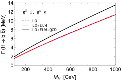
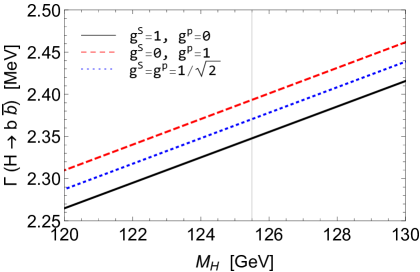
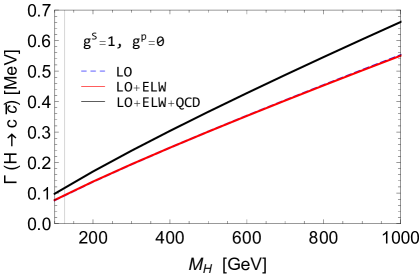
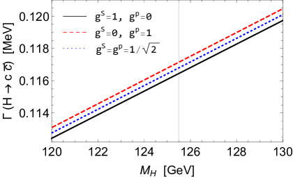
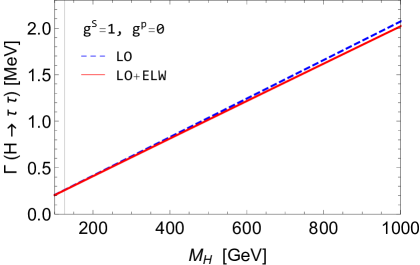
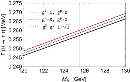
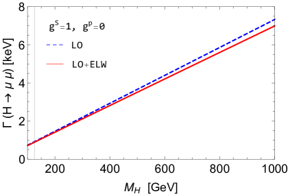
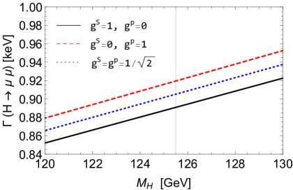
Figure 1: (Left) Decay widths of a neutral Higgs boson with mass $M_{H}$ into $b\bar{b}$, $c\bar{c}$, $\tau^{+}\tau^{-}$, and $\mu^{+}\mu^{-}$ from top to bottom taking $g^{S}_{H\bar{f}f}=1$ and $g^{P}_{H\bar{f}f}=0$. See the main text for details. (Right) In each row, the corresponding full decay widths are shown for the three choices of $(g^{S}_{H\bar{f}f}\,,g^{P}_{H\bar{f}f})=$ $(1,0)$ (solid), $(0,1)$ (dashed), and $(1/\sqrt{2},1/\sqrt{2})$ (dotted) in the low mass region around $M_{H}=125$ GeV. The vertical lines locate the positions of $M_{H}=125.5$ GeV. Note that the muonic decay widths are in units of keV.

In the left column of Fig. 1, taking $g^{S}_{H\bar{f}f}=1$ and $g^{P}_{H\bar{f}f}=0$, we show the decay widths of a Higgs boson $H$ into a pair of $b$ quarks, $c$ quarks, tau leptons, and muons for varying $M_{H}$. For the decays $H\to b\bar{b}$ and $H\to c\bar{c}$, the lower dashed lines are for the decay widths at leading order (LO) while the upper (black) solid lines are for those taking full account of the QCD and electroweak (ELW) corrections. The decay widths including only the electroweak corrections are denoted by the lower (red) solid lines. For the decays $H\to\tau^{+}\tau^{-}$ and $H\to\mu^{+}\mu^{-}$, the dashed lines are for the decay widths at LO and the sold lines are for the decay widths including the electroweak corrections. The behavior does not alter much for other choices of $(g^{S}_{H\bar{f}f}\,,g^{P}_{H\bar{f}f})$ as far as $|g^{S}_{H\bar{f}f}|^{2}+|g^{P}_{H\bar{f}f}|^{2}=1$ since the QCD correction $\delta_{\rm QCD}$, which is common in the scalar and pseudoscalar contributions to the Higgs decay width into quarks, dominates.

In each frame of the right column of Fig. 1, the corresponding full decay widths are shown in the low mass region of $120\,{\rm GeV}<M_{H}<130\,{\rm GeV}$ for the three choices of $(g^{S}_{H\bar{f}f}\,,g^{P}_{H\bar{f}f})=$ $(1,0)$, $(0,1)$, and $(1/\sqrt{2},1/\sqrt{2})$ denoted by the solid, dashed and dotted lines, respectively. The pure scalar case with $(g^{S}_{H\bar{f}f}\,,g^{P}_{H\bar{f}f})=(1,0)$ has a slightly smaller width compared to the pure pseudoscalar case with $(g^{S}_{H\bar{f}f}\,,g^{P}_{H\bar{f}f})=(0,1)$ due to the kinematical suppression factor of $\beta_{f}^{2}$.

At leading order (LO), taking the consideration of double off-shell effects, the decay width of a Higgs boson into a top-quark pair $t\bar{t}$, each of which subsequently decays into $bW^{+}$ and $\bar{b}W^{-}$, is given by [165, 166]

$$\Gamma^{\rm LO}(H\to t(p_{t})\,\bar{t}(\bar{p}_{t})\to b\bar{b}W^{+}W^{-})=N_{C}^{t}\frac{\overline{m}_{t}^{2}(M_{H})}{v^{2}}\frac{g^{4}M_{H}}{2^{13}\pi^{5}}\,{\cal F}\,,$$ (149)

where the dimensionless quantity ${\cal F}$ is given by an integrated function of the pole masses of $b$ and $t$ quarks, the $W$-boson mass, and the top-quark total width $\Gamma_{t}$ as [167]

$${\cal F} = \int\lambda_{H}^{1/2}\lambda_{t}^{1/2}\lambda_{\bar{t}}^{1/2}\left[|\lambda_{S}|^{2}\left|g^{S}_{H\bar{t}t}\right|^{2}+|\lambda_{P}|^{2}\left|g^{P}_{H\bar{t}t}\right|^{2}\right]\left(1+\frac{p_{t}^{2}+\bar{p}_{t}^{2}}{2M_{W}^{2}}+\frac{p_{t}^{2}\bar{p}_{t}^{2}}{4M_{W}^{4}}\right)$$ (150)

$$\hskip 71.13188pt\times\frac{p_{t}^{2}+M_{b}^{2}-M_{W}^{2}}{(p_{t}^{2}-M_{t}^{2})^{2}+M_{t}^{2}\Gamma_{t}^{2}}\ \frac{\bar{p}_{t}^{2}+M_{b}^{2}-M_{W}^{2}}{(\bar{p}_{t}^{2}-M_{t}^{2})^{2}+M_{t}^{2}\Gamma_{t}^{2}}\ d{p_{t}^{2}}\,d{\bar{p}_{t}^{2}}\,,$$

with the 5 dimensionless triangle functions

$$\lambda_{H} = 1+\frac{(p_{t}^{2})^{2}}{M_{H}^{4}}+\frac{(\bar{p}_{t}^{2})^{2}}{M_{H}^{4}}-2\frac{p_{t}^{2}}{M_{H}^{2}}-2\frac{\bar{p}_{t}^{2}}{M_{H}^{2}}-2\frac{p_{t}^{2}\bar{p}_{t}^{2}}{M_{H}^{4}}\,,$$

$$\lambda_{t} = \left(1-\frac{M_{b}^{2}}{p_{t}^{2}}-\frac{M_{W}^{2}}{p_{t}^{2}}\right)^{2}-4\frac{M_{b}^{2}}{p_{t}^{2}}\,\frac{M_{W}^{2}}{p_{t}^{2}}\,,$$

$$\lambda_{\bar{t}} = \left(1-\frac{M_{b}^{2}}{\bar{p}_{t}^{2}}-\frac{M_{W}^{2}}{\bar{p}_{t}^{2}}\right)^{2}-4\frac{M_{b}^{2}}{\bar{p}_{t}^{2}}\,\frac{M_{W}^{2}}{\bar{p}_{t}^{2}}\,,$$

$$\lambda_{S} = \left\{\left[(1+\lambda_{H}^{1/2})^{2}-(p_{t}^{2}-\bar{p}_{t}^{2})^{2}/M_{H}^{4}\right]^{1/2}-\left[(1-\lambda_{H}^{1/2})^{2}-(p_{t}^{2}-\bar{p}_{t}^{2})^{2}/M_{H}^{4}\right]^{1/2}\right\}/2\,,$$

$$\lambda_{P} = \left\{\left[(1+\lambda_{H}^{1/2})^{2}-(p_{t}^{2}-\bar{p}_{t}^{2})^{2}/M_{H}^{4}\right]^{1/2}+\left[(1-\lambda_{H}^{1/2})^{2}-(p_{t}^{2}-\bar{p}_{t}^{2})^{2}/M_{H}^{4}\right]^{1/2}\right\}/2\,.$$ (151)

After integrating over $p_{t}^{2}$ and $\bar{p}_{t}^{2}$, we can recast the LO decay width into

$$\Gamma^{\rm LO}(H\to t\,\bar{t}\to b\bar{b}W^{+}W^{-})\equiv\left|g^{S}_{H\bar{t}t}\right|^{2}\,{\cal T}^{\rm LO}_{S}+\left|g^{P}_{H\bar{t}t}\right|^{2}\,{\cal T}^{\rm LO}_{P}\,,$$ (152)

and, taking account of the radiative corrections as well as double off-shell effects, the Higgs decay width into a top quark pair $\Gamma(H\to t^{*}\bar{t}^{*})$ has been estimated as follows

$$\Gamma(H\to t^{*}\bar{t}^{*})=\left|g^{S}_{H\bar{t}t}\right|^{2}\,{\cal T}^{\rm LO}_{S}\left(1+\delta_{\rm QCD}+\delta^{t:S}_{t}+\delta^{t}_{\rm mixed}\right)\left(1+\delta^{t}_{\rm elw}\right)+\left|g^{P}_{H\bar{t}t}\right|^{2}\,{\cal T}^{\rm LO}_{P}\left(1+\delta_{\rm QCD}+\delta^{t:P}_{t}\right)\,.$$ (153)

When $M_{H}>2M_{t}$, taking $p^{2}_{t}=\bar{p}^{2}_{t}=M^{2}_{t}$ leads to $\lambda_{S}=\lambda_{H}^{1/2}=\beta_{t}=(1-4M_{t}^{2}/M_{H}^{2})^{1/2}$ and $\lambda_{P}=1$ and, neglecting the kinematical $b$-quark mass in the $t\to bW$ process, we reach the following factorized form for the LO decay width

$$\left.\Gamma^{\rm LO}(H\to t\,\bar{t}\to b\bar{b}W^{+}W^{-})\right|_{M_{H}>2M_{t}}=\Gamma^{\rm LO}(H\to t\bar{t})\,\left(\frac{\Gamma^{\rm LO}(t\to bW)}{\Gamma_{t}}\right)^{2}\,,$$ (154)

using the narrow-width approximation (NWA) denoted by

$$\delta(p^{2}-m^{2})=\lim_{\Gamma\to 0}\frac{m\Gamma}{\pi}\frac{1}{(p^{2}-m^{2})^{2}+m^{2}\Gamma^{2}}\,,$$ (155)

and the LO decay widths for $H\to t\bar{t}$ and $t\to bW$ given by

$$\Gamma^{\rm LO}(H\to t\bar{t}) = N_{C}^{t}\frac{\overline{m}_{t}^{2}(M_{H})}{v^{2}}\frac{\beta_{t}M_{H}}{8\pi}\left[\beta_{t}^{2}\left|g^{S}_{H\bar{t}t}\right|^{2}+\left|g^{P}_{H\bar{t}t}\right|^{2}\right]\,,$$ (156)

$$\Gamma^{\rm LO}(t\to bW) = \frac{g^{2}M_{t}}{2^{6}\pi}\left(1-\frac{M_{W}^{2}}{M_{t}^{2}}\right)^{2}\left(2+\frac{M_{t}^{2}}{M_{W}^{2}}\right)\,,$$ (157)

respectively.

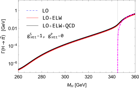
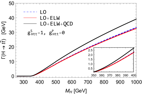
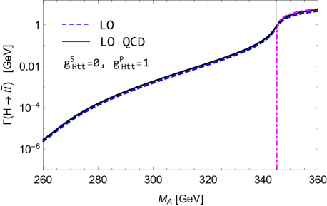
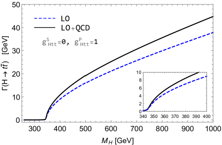
Figure 2: Decay widths of a neutral Higgs boson with mass $M_{H}$ into $t^{*}\bar{t}^{*}$ or $\Gamma(H\to t^{*}\bar{t}^{*})$ taking $(g^{S}_{H\bar{t}t},g^{P}_{H\bar{t}t})=(1,0)$ (upper) and $(g^{S}_{H\bar{t}t},g^{P}_{H\bar{t}t})=(0,1)$ (lower). In the left panels, the vertical lines locate the top-quark-pair thresholds and the (magenta) dash-dotted lines are for the corresponding full 2-body decay widths of $\Gamma(H\to t\bar{t})$. Note that, in the right panels, we switch from $\Gamma(H\to t^{*}\bar{t}^{*})$ to $\Gamma(H\to t\bar{t})$ from $M_{H}=500$ GeV and above.

In Fig. 2, we show the decay width $\Gamma(H\to t^{*}\bar{t}^{*})$ as a function of $M_{H}$, taking $(g^{S}_{H\bar{t}t},g^{P}_{H\bar{t}t})=(1,0)$ (upper) and $(g^{S}_{H\bar{t}t},g^{P}_{H\bar{t}t})=(0,1)$ (lower), respectively. We take $\Gamma_{t}=\Gamma^{\rm LO}(t\to bW)$ assuming that a top quark decays 100% into a $b$ quark and a $W$ boson and $\Gamma^{\rm LO}(H\to t\bar{t}\to b\bar{b}W^{+}W^{-})$ converges to $\Gamma^{\rm LO}(H\to t\bar{t})$ in the high $M_{H}$ limit. Practically, far above the top-quark-pair threshold with $M_{H}>500$ GeV, we return to Eq. (145) to suppress the contributions to $\Gamma(H\to t^{*}\bar{t}^{*})$ from the kinetic edge region of $\sqrt{p_{t}^{2}}+\sqrt{\bar{p}_{t}^{2}}\sim M_{H}$, assuming that the intermediate top quarks are reconstructed by requiring on-shell conditions of ${p_{t}^{2}}\simeq M_{t}^{2}$ and ${\bar{p}_{t}^{2}}\simeq M_{t}^{2}$.

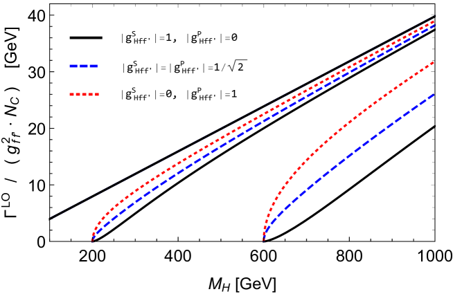
Figure 3: $\Gamma^{\rm LO}(H\to f\bar{f}^{\prime})/(g_{\bar{f}f^{\prime}}^{2}\,N_{C}^{ff^{\prime}})$ as functions of $M_{H}$ for the three choices of $(|g^{S}_{{}_{H\bar{f}f^{\prime}}}|,|g^{P}_{{}_{H\bar{f}f^{\prime}}}|)=(1,0)$ (black solid), $(|g^{S}_{{}_{H\bar{f}f^{\prime}}}|,|g^{P}_{{}_{H\bar{f}f^{\prime}}}|)=(1/\sqrt{2},1/\sqrt{2})$ (blue dashed), and $(|g^{S}_{{}_{H\bar{f}f^{\prime}}}|,|g^{P}_{{}_{H\bar{f}f^{\prime}}}|)=(0,1)$ (red dotted). We have taken $m_{f}=m_{f^{\prime}}=0\,,100\,,300$ GeV from left to right. Note that there is no dependence on the choice of the couplings when $m_{f}=m_{f^{\prime}}=0$ as far as $|g^{S}_{{}_{H\bar{f}f^{\prime}}}|^{2}+|g^{P}_{{}_{H\bar{f}f^{\prime}}}|^{2}$ remains the same.

Finally, for decays into two different fermions such as charginos or neutralinos or for flavor changing decays such as $H\to b\bar{s}$, one may write the effective interaction as

$${\cal L}_{H\bar{f}f^{\prime}}=-g_{\bar{f}f^{\prime}}H\bar{f}(g^{S}_{{}_{H\bar{f}f^{\prime}}}+ig^{P}_{{}_{H\bar{f}f^{\prime}}}\gamma_{5})f^{\prime}\ +\ {\rm h.c.}\,,$$ (158)

without loss of generality. Then, at LO, the decay width may take a form of

$$\Gamma^{\rm LO}(H\to f\bar{f}^{\prime})=N_{C}^{ff^{\prime}}\frac{g_{\bar{f}f^{\prime}}^{2}M_{H}\lambda^{1/2}_{ff^{\prime}}}{8\pi}\left[(1\!-\!\kappa\!-\!\kappa^{\prime})(|g^{S}_{{}_{H\bar{f}f^{\prime}}}|^{2}+|g^{P}_{{}_{H\bar{f}f^{\prime}}}|^{2})-2\sqrt{\kappa\kappa^{\prime}}(|g^{S}_{{}_{H\bar{f}f^{\prime}}}|^{2}-|g^{P}_{{}_{H\bar{f}f^{\prime}}}|^{2})\right]\,,$$ (159)

where $\kappa\equiv m_{f}^{2}/M_{H}^{2}$, $\kappa^{\prime}\equiv m_{f^{\prime}}^{2}/M_{H}^{2}$ and $\lambda_{ff^{\prime}}=(1-\kappa-\kappa^{\prime})^{2}-4\kappa\kappa^{\prime}$. The color factor $N_{C}^{ff^{\prime}}=3$ for quarks and 1 for leptons, charginos, and neutralinos. For the decays into neutralinos $\widetilde{\chi}^{0}_{j}$ and $\widetilde{\chi}^{0}_{k}$, we need to multiply the factor of $4/(1+\delta_{jk})$ with $\delta_{jk}=1$ for an identical Majorana neutralino pair. See Fig. 3 for the $M_{H}$ dependence of the normalized LO decay width $\Gamma^{\rm LO}(H\to f\bar{f}^{\prime})/(g_{\bar{f}f^{\prime}}^{2}\,N_{C}^{ff^{\prime}})$ for various choices of the couplings $|g^{S}_{{}_{H\bar{f}f^{\prime}}}|$ and $|g^{P}_{{}_{H\bar{f}f^{\prime}}}|$ and the fermion masses with $m_{f}=m_{f^{\prime}}$. When $m_{f}\neq m_{f^{\prime}}$, we observe that the LO decay width locates between the pseudoscalar (red dotted) and scalar (black solid) cases if the position of the mass threshold $m_{f}+m_{f^{\prime}}$ is the same. In this review, we consider the Higgs decays into SUSY particles only at LO. For the QCD and ELW corrections to them, we refer to Refs. [168, 169, 170, 171, 172].

3.2 Decays into two massive vector bosons: $H\to VV$ with $V=Z,W$

Taking the full consideration of double off-shell effects, the Higgs decay width into two massive vector bosons is given by [173, 165, 166, 174]

$$\Gamma^{\rm LO}(H\to V^{*}V^{*}) = \frac{1}{\pi^{2}}\int_{0}^{\omega_{V}}\frac{\epsilon_{V}{\rm d}y}{(y-1)^{2}+\epsilon_{V}^{2}}\int_{0}^{(\sqrt{\omega}_{V}-\sqrt{y})^{2}}\frac{\epsilon_{V}{\rm d}x}{(x-1)^{2}+\epsilon_{V}^{2}}$$ (160)

$$\times \frac{\delta_{V}g_{{}_{HVV}}^{2}G_{F}M_{H}^{3}}{16\sqrt{2}\pi}\,\lambda^{1/2}\left(1,\frac{x}{\omega_{V}},\frac{y}{\omega_{V}}\right)\left[\lambda\left(1,\frac{x}{\omega_{V}},\frac{y}{\omega_{V}}\right)+12\frac{xy}{\omega_{V}^{2}}\right]\,,$$

where $\delta_{W}=2$, $\delta_{Z}=1$, $\omega_{V}=1/\kappa_{V}=M_{H}^{2}/M_{V}^{2}$, $\epsilon_{V}=\Gamma_{V}/M_{V}$, and $\lambda(a,b,c)=(a-b-c)^{2}-4bc$. When $M_{V}<M_{H}<2M_{V}$ as in the case of the 125 GeV Higgs boson, the off-shell effects of one of the two vector bosons are negligible and the decay width reads [175]

$$\Gamma^{\rm LO}(H\to VV^{*})\, = \,\frac{\delta_{VV^{*}}}{\pi}\int_{0}^{(\sqrt{\omega}_{V}-1)^{2}}\frac{\epsilon_{V}{\rm d}x}{(x-1)^{2}+\epsilon_{V}^{2}}$$ (161)

$$\times \frac{\delta_{V}g_{{}_{HVV}}^{2}G_{F}M_{H}^{3}}{16\sqrt{2}\pi}\,\frac{1}{\omega_{V}^{3}}\,\lambda^{1/2}(\omega_{V},x,1)\left[\lambda(\omega_{V},x,1)+12x\right]\,,$$

with $\delta_{VV^{*}}=2$. See Fig. 4 for comparisons of $\Gamma^{\rm LO}(H\to V^{*}V^{*})$ and $\Gamma^{\rm LO}(H\to VV^{*})$. Incidentally, one may neglect all the off-shell effects for a heavy Higgs boson with $M_{H}>2M_{V}$ and the decay width takes a simple form:

$$\Gamma^{\rm LO}(H\to VV)=\frac{\delta_{V}g_{{}_{HVV}}^{2}G_{F}M_{H}^{3}}{16\sqrt{2}\pi}\,\beta_{V}\left[1-4\kappa_{V}+12\kappa_{V}^{2}\right]\,,$$ (162)

where $\beta_{V}=\sqrt{1-4\kappa_{V}}$ with $\kappa_{V}=M_{V}^{2}/M_{H}^{2}$.

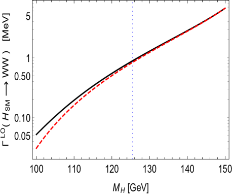
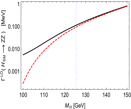
Figure 4: Comparisons of $\Gamma^{\rm LO}(H\to V^{*}V^{*})$ (solid) and $\Gamma^{\rm LO}(H\to VV^{*})$ (dashed). The vertical lines correspond to $M_{H}=125.5$ GeV and $g_{{}_{HVV}}=1$ is taken.

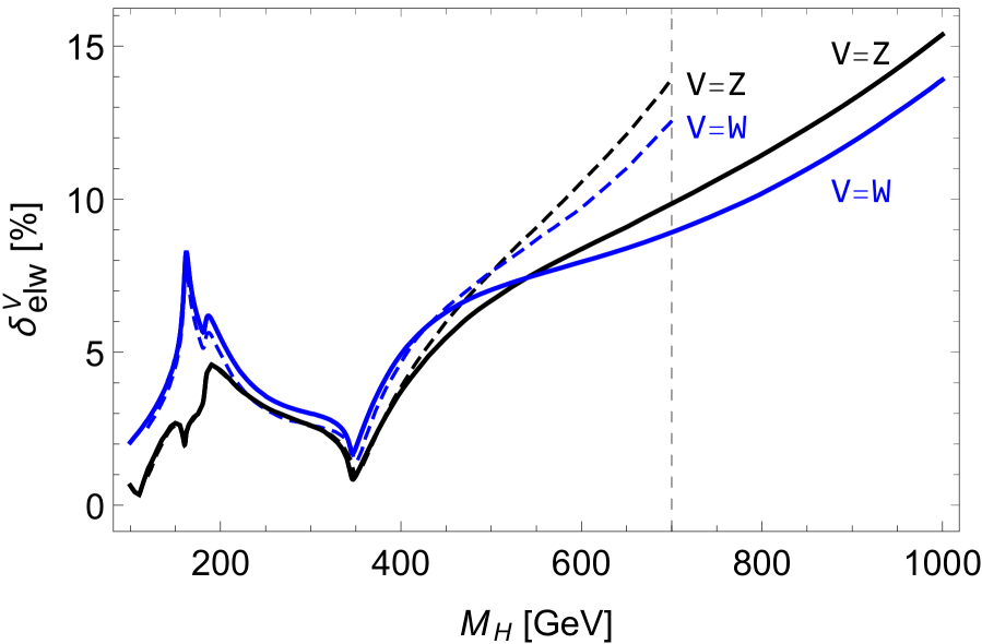
Figure 5: The electroweak correction factors $\delta^{V=Z,W}_{\rm elw}$ obtained from the complete electroweak corrections of ${\cal O}(\alpha)$ to the decay processes of $H\to ZZ\to e^{-}e^{+}\mu^{-}\mu^{+}$ ($V=Z$) and $H\to WW\to\nu_{e}e^{+}\mu^{-}\bar{\nu}_{\mu}$ ($V=W$). The dashed lines are obtained by combining the results presented in Figs. 7 and 8 of Ref. [91] while the solid lines by using the most recent version of PROPHECY4Fv3.0 taking the SM (or “model$=$0”) in the “inputfile”. For our numerical analyses, we adopt the solid lines by PROPHECY4Fv3.0.

Beyond the leading order, including radiative corrections and the double off-shell effects above as well as below the gauge-boson-pair thresholds, we estimate the radiatively–corrected decay width into two vector bosons by introducing a correction factor as

$$\Gamma(H\to VV\to 4f)=\Gamma^{\rm LO}(H\to V^{*}V^{*})\,\left(1+\delta^{V}_{\rm elw}\right)\,.$$ (163)

For the SM electroweak correction factors $\delta^{V=Z,W}_{\rm elw}$, we use the most recent version of PROPHECY4Fv3.0 [91, 176, 177, 178, 179, 180, 181] to calculate the complete ${\cal O}(\alpha)$ electroweak corrections to the Higgs decays into four fermions through intermediate $W$ and $Z$ bosons, supplemented by the corrections originating from heavy-Higgs effects and final-state radiation. We note that these electroweak corrections are applicable even near and below the gauge-boson-pair thresholds where the narrow-width approximation (NWA) is not applicable. The corrections amount to about 3% or less for $M_{H}=125$ GeV, as can be checked in Fig. 5. For the consistent implementation of the ELW corrections using PROPHECY4F, we note that one may need to adopt the complex pole masses of the $W$ and $Z$ bosons for the LO decay widths which are given by

$$M_{V}^{\rm pole}-i\Gamma^{\rm pole}_{V}=\frac{M_{V}-i\Gamma_{V}}{\sqrt{1+\Gamma_{V}^{2}/M_{V}^{2}}}\,.$$ (164)

Using the complex pole masses, we find that the LO decay width into $W^{*}W^{*}\,(Z^{*}Z^{*})$ increases by the amount of about 0.4% (0.5%) taking $M_{H}=125.5$ GeV, compared to those obtained using the on-shell masses and widths.

It has been estimated that missing corrections beyond ${\cal O}(\alpha)$ make the theoretical calculations for the inclusive decay rates into four fermions uncertain by the amount of 0.5% [182, 83].

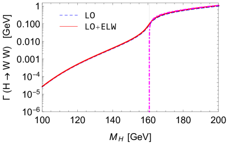
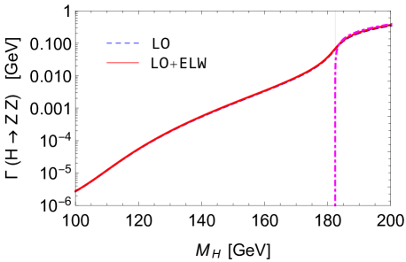
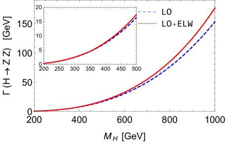
Figure 6: Decay widths of a neutral Higgs boson with mass $M_{H}$ into $W^{*}W^{*}$ (upper) and into $Z^{*}Z^{*}$ (lower) or $\Gamma(H\to VV\to 4f)$ taking $g_{{}_{HVV}}=1$. In the left panels, the vertical lines locate the vector-boson-pair thresholds and the (magenta) dash-dotted lines are for the corresponding 2-body decay widths of $\Gamma(H\to VV)=\Gamma^{\rm LO}(H\to VV)(1+\delta_{\rm elw}^{V})$.

In Fig. 6, we show the decay widths of a neutral Higgs boson with mass $M_{H}$ into $W^{*}W^{*}$ (upper) and into $Z^{*}Z^{*}$ (lower). Note that we include the electroweak corrections shown by the solid lines in Fig. 5. We observe that the electroweak corrections grow as $M_{H}$ increases and they make the partial decay widths into $WW$ and $ZZ$ as large as 350 GeV and 180 GeV, respectively, around $M_{H}=1$ TeV.

3.3 Decays into a lighter scalar boson and a vector boson and into two lighter scalar bosons: $H\to\varphi V\,,\varphi\varphi$

In the presence of multiple Higgs bosons, the decay of a heavier Higgs boson $H$ into a lighter neutral Higgs boson $\varphi$ and a massive gauge boson $Z$ may occur and, considering the case of a virtual $Z^{*}$, its decay width is given by an integral form as [173, 166, 174]

$$\Gamma^{\rm LO}(H\rightarrow\varphi Z^{*})=\frac{G_{F}M_{H}^{3}g_{{}_{H\varphi Z}}^{2}}{8\sqrt{2}\pi}\int_{0}^{(\sqrt{\omega}-\sqrt{\omega_{\varphi}})^{2}}{\rm d}x\frac{\epsilon_{Z}\lambda^{3/2}(\omega,\omega_{\varphi},x)}{\omega^{3}\pi[(x-1)^{2}+\epsilon_{Z}^{2}]}\,,$$ (165)

with $\omega=M_{H}^{2}/M_{Z}^{2}$ and $\omega_{\varphi}=M_{\varphi}^{2}/M_{Z}^{2}$. When $M_{H}$ is larger than $M_{\varphi}+M_{Z}$, using the $Z$-boson narrow-width approximation, it reduces to

$$\Gamma^{\rm LO}(H\to\varphi Z)\ =\ \frac{G_{F}M_{H}^{3}}{8\sqrt{2}\pi}g_{{}_{H\varphi Z}}^{2}\lambda^{3/2}(1,\kappa_{\varphi},\kappa_{Z})\,,$$ (166)

where $\kappa_{\varphi}=M_{\varphi}^{2}/M_{H}^{2}$ and $\kappa_{Z}=M_{Z}^{2}/M_{H}^{2}$. And, a heavier Higgs boson $H$ might also decay into a lighter charged Higgs boson $\varphi^{\pm}$ and a massive gauge boson $W^{\mp}$ with its decay width given by an integral form as [173, 166, 174]

$$\Gamma^{\rm LO}(H\rightarrow\varphi^{\pm}W^{\mp*})=\frac{G_{F}M_{H}^{3}|g_{{}_{H\varphi^{+}W^{-}}}|^{2}}{8\sqrt{2}\pi}\int_{0}^{(\sqrt{\omega}-\sqrt{\omega_{\pm}})^{2}}{\rm d}x\frac{\epsilon_{W}\lambda^{3/2}(\omega,\omega_{\pm},x)}{\omega^{3}\pi[(x-1)^{2}+\epsilon_{W}^{2}]}\,,$$ (167)

where $\Gamma^{\rm LO}(H\rightarrow\varphi^{\pm}W^{\mp*})=\Gamma^{\rm LO}(H\rightarrow\varphi^{+}W^{-*})=\Gamma^{\rm LO}(H\rightarrow\varphi^{-}W^{+*})$ with $\omega=M_{H}^{2}/M_{W}^{2}$ and $\omega_{\pm}=M_{\varphi^{\pm}}^{2}/M_{W}^{2}$. When $M_{H}$ is larger than $M_{\varphi^{\pm}}+M_{W}$, in the $W$-boson narrow-width approximation, it reduces to

$$\Gamma^{\rm LO}(H\to\varphi^{\pm}W^{\mp})\ =\ \frac{G_{F}M_{H}^{3}}{8\sqrt{2}\pi}|g_{{}_{H\varphi^{+}W^{-}}}|^{2}\lambda^{3/2}(1,\kappa_{\varphi},\kappa_{W})\,,$$ (168)

where $\kappa_{\varphi}=M_{\varphi^{\pm}}^{2}/M_{H}^{2}$ and $\kappa_{W}=M_{W}^{2}/M_{H}^{2}$.

Finally, when a heavier Higgs boson decays into a pair of lighter neutral Higgs bosons of $\varphi_{i}$ and $\varphi_{j}$ or into a pair of sfermions, at LO, we have for the decay width

$$\Gamma^{\rm LO}\ \left(H\to\varphi_{i}\varphi_{j}\,,\widetilde{f}^{*}_{i}\widetilde{f}_{j}\right)=\ N_{\varphi}\frac{v^{2}|{\cal G}|^{2}}{16\pi M_{H}}\lambda^{1/2}(1,\kappa_{i},\kappa_{j})\,,$$ (169)

where $(N_{\varphi},{\cal G})=(1+\delta_{ij},g_{{}_{H\varphi_{i}\varphi_{j}}})$ or $(N_{C}^{f},g_{H\widetilde{f}^{*}_{i}\widetilde{f}_{j}})$ and $\kappa_{i}=M_{\varphi_{i},\widetilde{f_{i}}}^{2}/M_{H}^{2}$. The decay width into a pair of lighter charged Higgs bosons is given by taking $(N_{\varphi},{\cal G})=(1,g_{{}_{HH^{+}H^{-}}})$. Again, the Higgs decays into SUSY particles are considered only at LO. In $H\to\varphi_{i}\varphi_{j}$ decay, we neglect the off-shell effects assuming $\Gamma_{\varphi}\sim\Gamma_{H_{\rm SM}}$ with a caution that the off-shell effects can not be neglected when the decay involves a transition between two heavy states with wide widths.

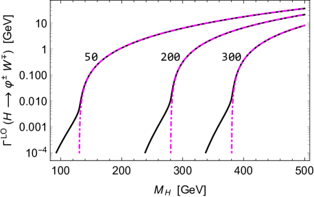
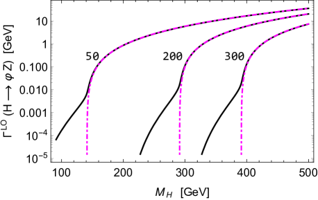
Figure 7: The LO decay widths of a neutral Higgs boson with mass $M_{H}$ into $\varphi^{-}W^{+*}$ (upper), $\varphi Z^{*}$ (middle), and $\varphi_{i}\varphi_{j}$ (lower) taking $|g_{{}_{H\varphi^{+}W^{-}}}|=1$, $g_{{}_{H\varphi Z}}=1$, and $N_{\varphi}|{\cal G}|^{2}=1$, respectively. In the upper and middle panels, the (magenta) dash-dotted lines are for the corresponding 2-body decay widths and we are taking $M_{\varphi}/{\rm GeV}=50\,,200$ , and $300$ from left to right. While in the lower panel, $M_{\varphi}/{\rm GeV}=50\,,100\,,200$ , and $300$ are taken.

In Fig. 7, we show the LO decay width of $\Gamma^{\rm LO}(H\to\varphi^{-}W^{+*})$ (upper) which is the same as $\Gamma^{\rm LO}(H\to\varphi^{+}W^{-*})$, $\Gamma^{\rm LO}(H\to\varphi Z^{*})$ (middle), and $\Gamma^{\rm LO}(H\to\varphi_{i}\varphi_{j})$ (lower). For the mass of a lighter scalar boson $\varphi$, we take three values of $50$ GeV, $200$ GeV, and $300$ GeV for $H\to\varphi V^{*}$ for illustration. For the decays $H\to\varphi_{i}\varphi_{j}$, we take $M_{\varphi_{i}}=M_{\varphi_{j}}=$ $50$ GeV, $100$ GeV, $200$ GeV, and $300$ GeV. All the relevant couplings are taken to be $1$ in the numerical analyses.

3.4 Decays into two gluons: $H\to gg$

By introducing two form factors, without loss of generality, the amplitude for the decay process $H\rightarrow gg$ can be written as

$${\cal M}_{ggH}^{ab}=-\frac{\alpha_{s}(M_{H})\,M_{H}^{2}\,\delta^{ab}}{4\pi\,v}\bigg{\{}S^{g}(M_{H})\left(\epsilon^{*}_{1\perp}\cdot\epsilon^{*}_{2\perp}\right)-P^{g}(M_{H})\frac{2}{M_{H}^{2}}\langle\epsilon^{*}_{1}\epsilon^{*}_{2}k_{1}k_{2}\rangle\bigg{\}}\,,$$ (170)

where $a$ and $b$ ($a,b=1$ to 8) are indices of the eight generators in the SU(3) adjoint representation, $k_{1,2}$ the four momenta of the two gluons and $\epsilon_{1,2}$ the wave vectors of the corresponding gluons, $\epsilon^{\mu}_{1\perp}=\epsilon^{\mu}_{1}-2k^{\mu}_{1}(k_{2}\cdot\epsilon_{1})/M^{2}_{H}$, $\epsilon^{\mu}_{2\perp}=\epsilon^{\mu}_{2}-2k^{\mu}_{2}(k_{1}\cdot\epsilon_{2})/M^{2}_{H}$ and $\langle\epsilon_{1}\epsilon_{2}k_{1}k_{2}\rangle\equiv\epsilon_{\mu\nu\rho\sigma}\,\epsilon_{1}^{\mu}\epsilon_{2}^{\nu}k_{1}^{\rho}k_{2}^{\sigma}$. Retaining only the dominant contributions from third–generation quarks and introducing $\Delta S^{g}$ and $\Delta P^{g}$ to parameterize contributions from the triangle loops in which non-SM colored particles are running, the scalar and pseudoscalar form factors are given by

$$S^{g}(M_{H})=\sum_{f=b,t,c}g^{S}_{H\bar{f}f}\,F_{sf}(\tau_{f})+\Delta S^{g}\,;\ \ \ P^{g}(M_{H})=\sum_{f=b,t,c}g^{P}_{H\bar{f}f}\,F_{pf}(\tau_{f})+\Delta P^{g}\,,$$ (171)

where $\tau_{f}\equiv M_{H}^{2}/4M_{f}^{2}$ is defined by using the pole masses of the bottom and top quarks. The form factors $F_{sf}$ and $F_{pf}$ can be expressed by

$$F_{sf}(\tau) = \tau^{-1}\,[1+(1-\tau^{-1})f(\tau)]\,,~{}~{}F_{pf}(\tau)=\tau^{-1}\,f(\tau)\,,$$ (172)

in terms of a so-called scaling function $f(\tau)$ which stands for the integral function

$$f(\tau)=-\frac{1}{2}\int_{0}^{1}\frac{{\rm d}y}{y}\ln\left[1-4\tau y(1-y)\right]=\left\{\begin{array}[]{cl}{\rm arcsin}^{2}(\sqrt{\tau})\,:&\qquad\tau\leq 1\,,\\ -\frac{1}{4}\left[\ln\left(\frac{\sqrt{\tau}+\sqrt{\tau-1}}{\sqrt{\tau}-\sqrt{\tau-1}}\right)-i\pi\right]^{2}\,:&\qquad\tau\geq 1\,.\end{array}\right.$$ (175)

It is clear that the imaginary parts of the form factors appear for Higgs-boson masses greater than twice the mass of the colored particle running in the loop, i.e., $\tau\geq 1$. In the limit $\tau\rightarrow 0$, $F_{sf}(0)=2/3$ and $F_{pf}(0)=1$, see Fig. 8.

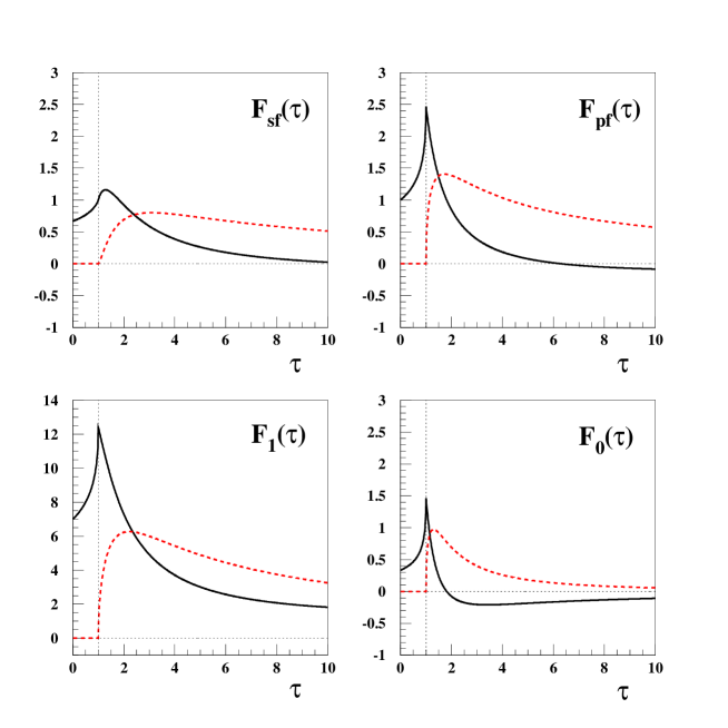
Figure 8: Behavior of the real (solid) and imaginary (dashed) parts of the four form factors of $F_{sf}$, $F_{pf}$, $F_{1}$ and $F_{0}$ versus $\tau=s/4m^{2}$ with $\sqrt{s}=M_{H}$ and $m$ being the mass of the particle running in the triangle loops. The form factors are defined explicitly in the main text where they first appear, see Eqs. (172), (183), and (B.3). The vertical lines denote the mass threshold above which $M_{H}>2m$.

The decay width of the process $H\rightarrow gg$ may be cast into the form

$$\Gamma(H\rightarrow gg)\ =\ \frac{M_{H}^{3}\alpha^{2}_{S}}{32\pi^{3}\,v^{2}}\left[\left|S^{g}(M_{H})\right|^{2}\,\left(1+\delta^{g:S}_{\rm QCD}\right)\left(1+\delta^{g:S}_{\rm elw}\right)+\left|P^{g}(M_{H})\right|^{2}\,\left(1+\delta^{g:P}_{\rm QCD}\right)\left(1+\delta^{g:P}_{\rm elw}\right)\right]\,,$$ (176)

including the QCD and electroweak corrections. The two corrections are factorized as dictated by the universal infrared and collinear behavior of QCD corrections and the universality of the dominant part of ELW corrections. The QCD correction of $\delta^{g:S}_{\rm QCD}$ is known up to NLO including the full quark mass dependence [183] and up to the N³LO in the limit of heavy top quarks [184, 185, 186]:

$$\delta^{g:S}_{\rm QCD} = \left(\frac{95}{4}-\frac{7}{6}N_{F}^{L}+\Delta^{g:S}_{m}\right)\frac{\alpha_{s}^{(N_{F}^{L})}(M_{H})}{\pi}$$ (177)

$$+ \left[370.20-47.19N_{F}^{L}+0.902(N_{F}^{L})^{2}+(2.375+0.667N_{F}^{L})\log\frac{M_{H}^{2}}{M_{t}^{2}}\right]\left(\frac{\alpha_{s}^{(N_{F}^{L})}(M_{H})}{\pi}\right)^{2}$$

$$+ \left[4533.46-1062.82N_{F}^{L}+52.62(N_{F}^{L})^{2}-0.5378(N_{F}^{L})^{2}\phantom{\log\frac{M_{H}^{2}}{M_{t}^{2}}}\right.$$

$$\,+(66.66+14.60N_{F}^{L}-0.6887(N_{F}^{L})^{2})\log\frac{M_{H}^{2}}{M_{t}^{2}}$$

$$\left.+(6.53+1.44N_{F}^{L}-0.111(N_{F}^{L})^{2})\log^{2}\frac{M_{H}^{2}}{M_{t}^{2}}\right]\left(\frac{\alpha^{(N_{F}^{L})}_{s}(M_{H})}{\pi}\right)^{3}\,,$$

with $N_{F}^{L}=5$ counting the flavor number of light quarks and $\Delta^{g:S}_{m}\approx 0.7$ for the NLO quark-mass effects from the top, bottom and charm quarks [183]. Taking $M_{H}=125.5$ GeV, we find $\delta^{g:S}_{\rm QCD}=0.67+0.20+0.02$ for the NLO, NNLO, and N³LO corrections. On the other hand, the QCD corrections to the pseudoscalar part develop a Coulomb singularity at the top-quark-pair threshold which can be regularized by including the finite top decay width [187, 188, 189, 190]. The correction $\delta^{g:P}_{\rm QCD}$ is known up to NNLO in the limit of heavy top quarks [191] while the NLO corrections are known exactly [183]:

$$\delta^{g:P}_{\rm QCD} = \left(\frac{97}{4}-\frac{7}{6}N_{F}^{L}+\Delta_{m}^{g:P}\right)\frac{\alpha^{(N_{F}^{L})}_{s}(M_{H})}{\pi}$$ (178)

$$+ \left(392.22-48.58N_{F}^{L}+0.888(N_{F}^{L})^{2}+N_{F}^{L}\log\frac{M_{H}^{2}}{M_{t}^{2}}\right)\left(\frac{\alpha^{(N_{F}^{L})}_{s}(M_{H})}{\pi}\right)^{2}\,,$$

with $\Delta^{g:P}_{m}\approx 0.04$ for $\tan\beta=1$, for example, in the MSSM. Taking $M_{H}=125.5$ GeV, we find $\delta^{g:P}_{\rm QCD}\simeq 0.66+0.22$ for the NLO and NNLO terms. We note that $\delta^{g:P}_{\rm QCD}$ is derived in the heavy top-quark limit and it does not contain the Coulomb singularity.

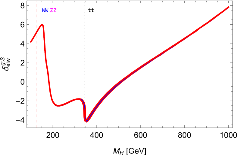
Figure 9: Behavior of the two-loop SM electroweak corrections of $\delta^{g:S}_{\rm elw}$ for $\Gamma(H\to gg)$ versus $M_{H}$. The vertical lines locate $M_{H}=125.5$ GeV and the $WW$, $ZZ$, and $t\bar{t}$ thresholds. The line width represents uncertainties taking account of $M_{t}=172.64\pm 1.58$ GeV. From the authors of Refs. [198, 197, 199, 200]. See also Refs. [201, 196, 194].

The electroweak corrections $\delta^{g:S}_{\rm elw}$ of ${\cal O}(G_{F}M_{t}^{2})$ are given by [163, 192, 193]

$$\delta^{g:S}_{\rm elw}=\frac{G_{F}M_{t}^{2}}{8\sqrt{2}\pi^{2}}\,.$$ (179)

Note that these ${\cal O}(G_{F}M_{t}^{2})$ electroweak corrections increase the gluonic decay width only by the amount of about $0.3$%. It turns out that the full electroweak corrections [194, 195, 196, 197, 198] lead to much more significant enhancement of $\delta^{g:S}_{\rm elw}\sim 5$% below the $WW$ threshold, see Fig. 9. On the other hand, the other electroweak corrections $\delta^{g:P}_{\rm elw}$ may be given by [202, 203]

$$\delta^{g:P}_{\rm elw}\simeq-\left(7+\eta^{g:P}_{\rm elw}\right)\frac{G_{F}M_{t}^{2}}{8\sqrt{2}\pi^{2}}\,,$$ (180)

where the first factor of $7$ counts the contribution of the SU(2)_L doublet which, in the decoupling limit, plays the role of the SM SU(2)_L doublet including the 125 GeV Higgs boson. And the second factor of $\eta^{g:P}_{\rm elw}$ denotes the model-dependent BSM contribution. In the type-II 2HDM, for example, it is given by $\eta^{g:P}_{\rm elw}=10/\tan^{2}\beta$ in the infinite top quark mass approximation [203]. These electroweak corrections reduce the gluonic decay width at the percent level. Note that Eq. (180) is a crude approximation obtained by focusing on the top-Yukawa contributions which are subleading in the SM. The same arguments apply for Eq. (179) which we are not using for our numerical study though.

We have addressed all the known QCD and electroweak corrections to the decay width of a neutral Higgs boson into two gluons. The theoretical uncertainties due to the unknown higher-order QCD and NLO electroweak corrections are estimated as 3% and 1%, respectively [182, 84].

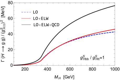
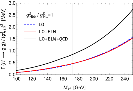
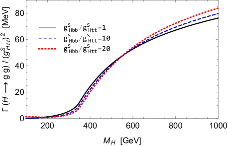
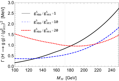
Figure 10: (Upper) Normalized decay widths of a neutral Higgs boson with mass $M_{H}$ into $gg$ taking $g^{S}_{H\bar{b}b}/g^{S}_{H\bar{t}t}=1$, $\Delta S^{g}=0$, and $g^{P}_{H\bar{q}q}=\Delta P^{g}=0$. In the right panel, the low $M_{H}$ region is magnified. The LO (blue dashed), LO$+$ELW (lower red solid), and LO$+$ELW$+$QCD (upper black solid) results are separately shown. (Lower) The same as in the upper panels but for three values of $g^{S}_{H\bar{b}b}/g^{S}_{H\bar{t}t}=1\,,10$ , and $20$ taking full account of the electroweak and QCD corrections. The vertical lines in the right panels locate the position $M_{H}=M_{t}$.

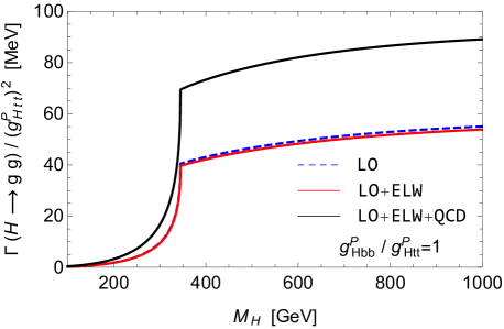
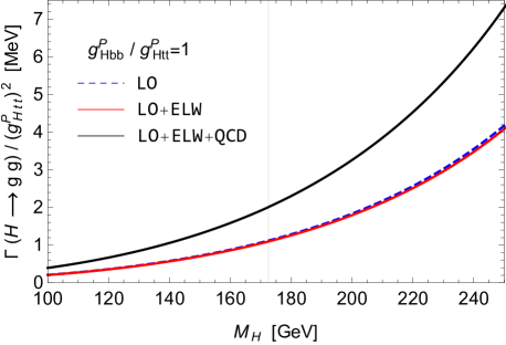
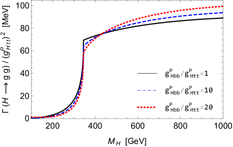
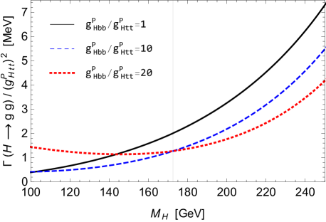
Figure 11: The same as in Fig. 10 while taking $g^{S}_{H\bar{q}q}=0$ and $g^{P}_{H\bar{q}q}\neq 0$ with $\Delta S^{g}=\Delta P^{g}=0$.

In the upper panels of Fig. 10, we show the normalized decay widths $\Gamma(H\to gg)/(g^{S}_{H\bar{t}t})^{2}$ at LO (blue dashed), including only the electroweak corrections (red solid), and including both the electroweak and QCD corrections (black solid). We assume that all the pseudo-scalar couplings of $g^{P}_{H\bar{q}q}$ are vanishing and $\Delta S^{g}=0$. The electroweak corrections $\delta^{g:S}_{\rm elw}$ are directly read off from Fig. 9. In the right panel, we magnify the low $M_{H}$ region and locate the position $M_{H}=M_{t}$ with a thin vertical line. In the lower panels, we show the normalized decay widths including the available electroweak and QCD corrections and taking three values of $g^{S}_{H\bar{b}b}/g^{S}_{H\bar{t}t}=1$ (black solid), $10$ (blue dashed), and $20$ (red dotted), considering the situation in which the bottom Yukawa coupling is enhanced as in the 2HDM II for large $\tan\beta$. Note that the black solid lines in the lower panels are the same as those in the upper ones.

In Fig. 11, the alternative choice is made to show $\Gamma(H\to gg)/(g^{P}_{H\bar{t}t})^{2}$ assuming all the scalar couplings of $g^{S}_{H\bar{q}q}$ are vanishing and $\Delta P^{g}=0$. For the electroweak corrections $\delta^{g:P}_{\rm elw}$, we take $\eta^{g:P}_{\rm elw}=0$. Compared to the scalar case in which the form factor $f_{sf}(\tau)$ is involved, the rise near the top-quark-pair threshold is sharper and bigger due to the behavior of the real and imaginary parts of the form factor $f_{pf}(\tau)$ around $\tau=1$, see Fig. 8. In the low $M_{H}$ region, we find that the decay widths are larger by about the factor of $[f_{pf}(0)/f_{sf}(0)]^{2}\sim 2$ when the $b$-quark contributions are neglected. As the coupling ratios $g^{S,P}_{H\bar{b}b}/g^{S,P}_{H\bar{t}t}$ increase, the contributions from $b$-quark loops become comparable to and larger than those from $t$-quark loops and, in this case, the decay widths are nearly the same especially around $M_{H}=100$ GeV as can be checked with the dashed and dotted lines in the lower-right panels of Figs. 10 and 11.

3.5 Decays into two photons: $H\to\gamma\gamma$

The amplitude for the radiative decay process $H\rightarrow\gamma\gamma$, playing a crucial role in the discovery of the Higgs boson at the LHC, can be written as

$${\cal M}_{\gamma\gamma H}=-\frac{\alpha(0)M_{H}^{2}}{4\pi\,v}\bigg{\{}S^{\gamma}(M_{H})\,\left(\epsilon^{*}_{1\perp}\cdot\epsilon^{*}_{2\perp}\right)-P^{\gamma}(M_{H})\frac{2}{M_{H}^{2}}\langle\epsilon^{*}_{1}\epsilon^{*}_{2}k_{1}k_{2}\rangle\bigg{\}}\,,$$ (181)

in terms of the two form factors of $S^{\gamma}$ and $P^{\gamma}$. Here $k_{1,2}$ and $\epsilon_{1,2}$ are the four–momenta and wave vectors of the two photons, respectively, as in the decay $H\rightarrow gg$. Note that the electromagnetic fine structure constant in the coupling should be taken at the scale $q^{2}=0$ since the final–state photons are real. Retaining only the dominant contributions from third–generation fermions and the charged gauge bosons $W^{\pm}$ and introducing two residual form factors $\Delta S^{\gamma}$ and $\Delta P^{\gamma}$ to parameterize contributions from the triangle loops in which non-SM charged particles are running, the scalar and pseudoscalar form factors are given by

$$S^{\gamma}(M_{H}) = 2\sum_{f=b,t,\tau}N_{C}^{f}\,Q_{f}^{2}\,g^{S}_{H\bar{f}f}\,F_{sf}(\tau_{f})-g_{{}_{HWW}}F_{1}(\tau_{W})+\Delta S^{\gamma}\,;$$

$$P^{\gamma}(M_{H}) = 2\sum_{f=b,t,\tau}N_{C}^{f}\,Q_{f}^{2}\,g^{P}_{H\bar{f}f}\,F_{pf}(\tau_{f})+\Delta P^{\gamma}\,,$$ (182)

where $N_{C}^{f}=3$ for quarks and $N_{C}^{f}=1$ for charged leptons, respectively. For the $\tau$ lepton and the $W$ boson, $\tau_{\tau}=M_{H}^{2}/4M_{\tau}^{2}$ and $\tau_{W}=M_{H}^{2}/4M_{W}^{2}$, respectively. On the other hand, for quarks, $\tau_{q}$ is defined in terms of the running quark mass at the scale of $M_{H}/2$, i.e. $\tau_{q}=M_{H}^{2}/4[m_{q}(M_{H}/2)]^{2}$ where $m_{q}$ is normalized as $m_{q}(M_{q})=M_{q}$. Note that the choice of the scale $\mu_{q}=M_{H}/2$ correctly gives $m_{q}(M_{H}/2)=M_{q}$ at the threshold where $M_{H}=2M_{q}$ and makes the full two-loop QCD corrections remain small in the entire range of the variable $\tau_{q}$ by effectively absorbing all relevant large logarithms into the running mass. The form factor $F_{1}$ is given by

$$F_{1}(\tau)=2+3\tau^{-1}+3\tau^{-1}(2-\tau^{-1})f(\tau)\,,$$ (183)

which takes the value of 7 in the limit $\tau\to 0$, see Fig. 8 for the $\tau$ dependence of the form factor. At LO, the decay width of the radiative process is given by

$$\Gamma^{\rm LO}(H\rightarrow\gamma\gamma)=\frac{M_{H}^{3}\alpha^{2}}{256\pi^{3}\,v^{2}}\left[\,\left|S^{\gamma}(M_{H})\right|^{2}+\left|P^{\gamma}(M_{H})\right|^{2}\right]\,,$$ (184)

with the fine structure constant $\alpha=\alpha(0)\simeq 1/137$.

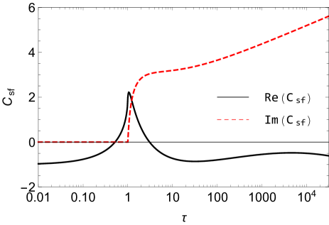
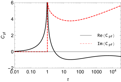
Figure 12: Behavior of the real (solid) and imaginary (dashed) parts of the scaling factors $C_{sf}(\tau)$ (left) and $C_{pf}(\tau)$ (right) for the QCD corrections to the decay of a Higgs boson into two photons.

As a gluon cannot be radiated from the colored quark loop contributing to the $H\gamma\gamma$ vertex owing to charge conjugation invariance and color conservation, the full two-loop QCD corrections [183, 204, 205, 206, 207, 208, 209, 210, 211, 212, 213, 214, 215, 216] can be taken into account by simply introducing the scaling factors in the form factors for the $b$- and $t$-quark contributions as:

$$F_{sf}(\tau_{q}) \longrightarrow F_{sf}(\tau_{q})\,\left[1+C_{sf}(\tau_{q})\frac{\alpha_{s}(M_{H})}{\pi}\right]\,;$$

$$F_{pf}(\tau_{q}) \longrightarrow F_{pf}(\tau_{q})\,\left[1+C_{pf}(\tau_{q})\frac{\alpha_{s}(M_{H})}{\pi}\right]\,.$$ (185)

The scaling factors $C_{sf}$ and $C_{pf}$ approach $-1$ and $0$, respectively, in the limit $\tau\rightarrow 0$, see Fig. 12.

The asymptotic values of the scalar and pseudoscalar scaling factors in the heavy quark limit, $C_{sf}(0)=-1$ and $C_{pf}(0)=0$, can also be deduced by means of a general low-energy theorem for amplitudes involving soft Higgs particles. According to the low-energy theorem, the NLO QCD corrections to the scalar coupling to two photons in the heavy quark limit can be obtained from the effective Lagrangian [86, 183, 217, 218, 219]

$${\cal L}^{S}_{\rm eff}=g^{S}_{H\bar{q}q}\,\frac{Q^{2}_{q}}{4}\frac{\beta^{q}_{\rm QED}/\alpha}{1+\gamma_{m}(\alpha_{s})}\,F^{\mu\nu}F_{\mu\nu}\,\frac{H}{v}\,,$$ (186)

where the QED $\beta$ function $\beta^{q}_{\rm QED}/\alpha=2(\alpha/\pi)[1+\alpha_{s}/\pi+\cdots]$ with the heavy quark $q$ contribution and the anomalous mass dimension $\gamma_{m}=2\alpha_{s}/\pi+\cdots$ [220]. Therefore, the NLO expansion of the effective Lagrangian of the scalar coupling to two photons reads

$${\cal L}^{S}_{\rm eff}=g^{S}_{H\bar{q}q}\,Q^{2}_{q}\frac{\alpha}{2\pi}F^{\mu\nu}F_{\mu\nu}\left[1-\frac{\alpha_{s}}{\pi}+{\cal O}(\alpha^{2}_{s})\right]\,\frac{H}{v}\,,$$ (187)

which agrees with the asymptotic value of $C_{sf}(0)=-1$ in the heavy quark limit. On the other hand, the pseudoscalar scaling factor is zero in the heavy quark limit, i.e., $C_{pf}(0)=0$, because the QCD corrections to the pseudoscalar decay mode vanish in this limit due to the Adler-Bardeen theorem [221]. The effective Lagrangian for the pseudoscalar coupling to two photons can be derived from the Adler-Bell-Jackiw (ABJ) anomaly in the divergence of the axial vector current [222, 223] and is given to all orders of the perturbation theory by [86, 183]

$${\cal L}^{P}_{\rm eff}=g^{P}_{H\bar{q}q}\,Q^{2}_{q}\,\frac{3\alpha}{4\pi}\,F^{\mu\nu}\widetilde{F}_{\mu\nu}\,\frac{H}{v}\,,$$ (188)

for the pseudoscalar boson, as the lowest order axial-anomaly term is not renormalized at all orders.

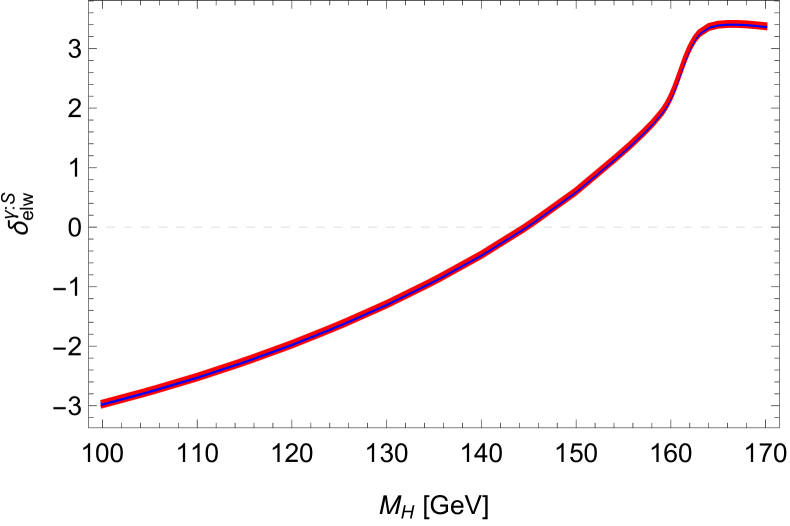
Figure 13: The two-loop electroweak corrections $\delta_{\rm elw}^{\gamma:S}$ to the part of the decay width of a Higgs boson into two photons via the scalar form factor in the full complex-mass scheme which has been designed to cure the unphysical infinities of two-loop amplitudes [198]. The line width represents uncertainties taking account of $M_{t}=172.64\pm 1.58$ GeV. From the authors of Refs. [198, 197, 199, 200].

The two-loop electroweak corrections of $\delta^{\gamma:S}_{\rm elw}$ to the scalar part of the decay width via the scalar form factor have been calculated in Refs. [198, 224, 201, 200], see Fig. 13. The electroweak corrections to the pseudoscalar part are also available [202, 203]:

$$\delta^{\gamma:P}_{\rm elw}=-\frac{G_{F}M_{t}^{2}}{8\sqrt{2}\pi^{2}}\left(4+\eta^{\gamma:P}_{\rm elw}\right)\,,$$ (189)

where, similarly as in the decay $H\to gg$, the factor $4$ counts the contribution of the SM SU(2)_L doublet in the decoupling limit and $\eta^{\gamma:P}_{\rm elw}$ the model-dependent BSM contribution. In the type-II 2HDM, for example, $\eta^{\gamma:P}_{\rm elw}=7/\tan^{2}\beta$ in the infinite top quark mass approximation [202, 203], suppressed for large $\tan\beta$. Note again that Eq. (189) is a crude approximation obtained by focusing on the top-Yukawa contributions which are subleading in the SM.

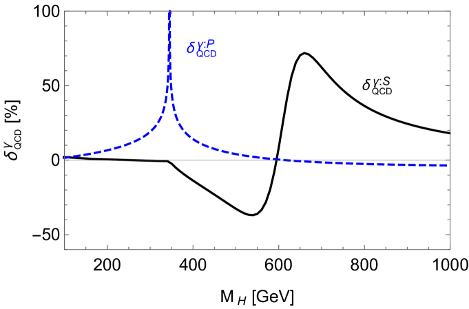
Figure 14: Behavior of the two-loop QCD corrections to the decay width of a Higgs boson into two photons: $\delta^{\gamma:S}_{\rm QCD}$ (solid) and $\delta^{\gamma:P}_{\rm QCD}$ (dashed). We take $g_{{}_{HWW}}=g^{S}_{H\bar{t}t}=g^{S}_{H\bar{b}b}=g^{S}_{H\tau\tau}=1$ for $\delta^{\gamma:S}_{\rm QCD}$ while $g^{P}_{H\bar{b}b}=g^{P}_{H\tau\tau}=0$ for $\delta^{\gamma:P}_{\rm QCD}$. Both of the residual form factors $\Delta S^{\gamma}$ and $\Delta P^{\gamma}$ are taken to be vanishing.

Incorporating all the QCD and electroweak corrections, one may write

$$\Gamma(H\rightarrow\gamma\gamma)=\frac{M_{H}^{3}\alpha^{2}}{256\pi^{3}\,v^{2}}\left[\,\left|S^{\gamma}(M_{H})\right|^{2}\left(1+\delta^{\gamma:S}_{\rm QCD}\right)\left(1+\delta^{\gamma:S}_{\rm elw}\right)+\left|P^{\gamma}(M_{H})\right|^{2}\left(1+\delta^{\gamma:P}_{\rm QCD}\right)\left(1+\delta^{\gamma:P}_{\rm elw}\right)\right]\,.$$ (190)

Note that the electroweak corrections are directly from Fig. 13 and Eq. (189) while the QCD corrections enter through the scaling factors $C_{sf}(\tau_{q})$ and $C_{pf}(\tau_{q})$. For $M_{H}=125.5$ GeV, the QCD corrections $\delta^{\gamma:S}_{\rm QCD}$ increase the decay width into two photons by about 2%. On the other hand, the electroweak corrections $\delta^{\gamma:S}_{\rm elw}$ decrease the decay width by about 2% , almost canceling the NLO QCD corrections to the corresponding part. In Fig. 14, we show the QCD corrections $\delta^{\gamma:S}_{\rm QCD}$ (solid) and $\delta^{\gamma:P}_{\rm QCD}$ (dashed) with varying $M_{H}$. For the scalar QCD correction $\delta^{\gamma:S}_{\rm QCD}$, we take the SM values of $g_{{}_{HWW}}=g^{S}_{H\bar{t}t}=g^{S}_{H\bar{b}b}=g^{S}_{H\tau\tau}=1$ with $\Delta S^{\gamma}=0$. While, for the pseudoscalar QCD correction $\delta^{\gamma:P}_{\rm QCD}$, we assume a scenario in which the pseudoscalar form factor $P^{\gamma}$ is dominated by the top-quark contribution taking $g^{P}_{H\bar{b}b}=g^{P}_{H\tau\tau}=\Delta P^{\gamma}=0$. At $M_{H}=2M_{t}$, the pseudoscalar QCD correction $\delta^{\gamma:P}_{\rm QCD}$ diverges due to the singular property of $C_{pf}$ at $\tau=1$. Around $M_{H}=600$ GeV where the large cancellation occurs between the $W$-boson and top-quark contributions, the scalar QCD correction $\delta^{\gamma:S}_{\rm QCD}$ is relatively large and it could vary between about $-0.4$ and $0.8$.

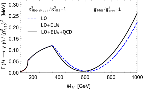
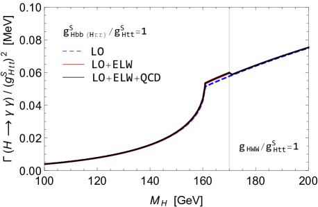
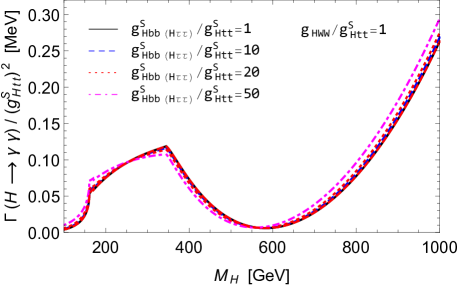
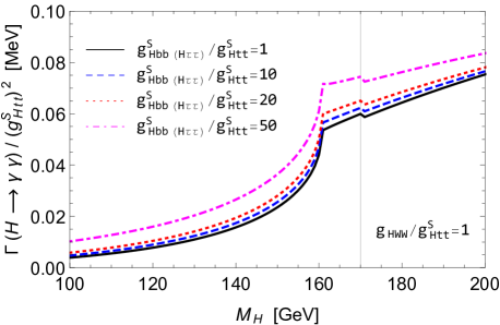
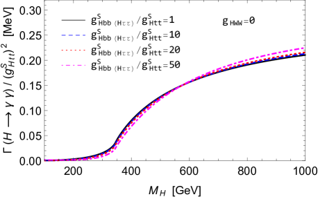
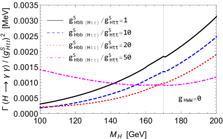
Figure 15: (Upper) Normalized decay widths of a neutral Higgs boson with a mass $M_{H}$ into $\gamma\gamma$ taking $g_{{}_{HWW}}/g^{S}_{H\bar{t}t}=g^{S}_{H\bar{b}b\,,H\tau\tau}/g^{S}_{H\bar{t}t}=1$ and $g^{P}_{H\bar{f}f}=0$. In the right panel, the low $M_{H}$ region is magnified. The LO (blue dashed), LO$+$ELW (red solid), and LO$+$ELW$+$QCD (black solid) results are separately shown. (Middle) The same as in the upper panels but for the four values of $g^{S}_{H\bar{b}b}/g^{S}_{H\bar{t}t}=1\,,10\,,20$ , and $50$ taking full account of the electroweak and QCD corrections. $g_{{}_{HWW}}/g^{S}_{H\bar{t}t}=1$ is taken. (Lower) The same as in the middle panels but with $g_{{}_{HWW}}=0$. The vertical lines in the right panels locate the position $M_{H}=170$ GeV beyond which the electroweak corrections are ignored. In all panels, we take $\Delta S^{\gamma}=\Delta P^{\gamma}=0$.

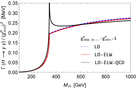
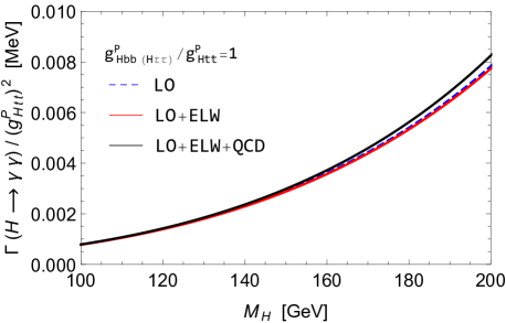
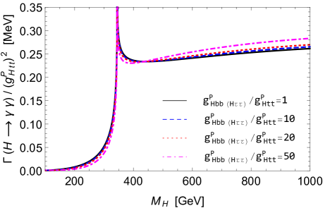
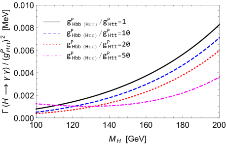
Figure 16: Normalized decay widths of a neutral Higgs boson with a mass $M_{H}$ into $\gamma\gamma$ via the pseudoscalar form factor $P^{\gamma}$ with $\Delta P^{\gamma}=0$. In this case, only the fermion couplings of $g^{P}_{H\bar{f}f}$ with $f=t,b,\tau$ are relevant.

In the upper panels of Fig. 15, we show the decay width of a neutral Higgs boson into two photons normalized to the $g_{H\bar{t}t}$ coupling squared taking $g_{{}_{HWW}}/g^{S}_{H\bar{t}t}=g^{S}_{H\bar{b}b\,,H\tau\tau}/g^{S}_{H\bar{t}t}=1$ and $g^{P}_{H\bar{f}f}=\Delta S^{\gamma}=\Delta P^{\gamma}=0$. This reduces to the SM decay width of a Higgs particle with mass $M_{H}$ when $g_{H\bar{t}t}=1$. For $M_{H}\leq 170$ GeV, we apply the electroweak corrections $\delta_{\rm elw}^{\gamma:S}$ directly read off from Fig. 13 and we simply neglect them above $M_{H}=170$ GeV, expecting the electroweak corrections to be evaluated with high precision for heavy Higgs bosons if necessary. Below the $W$-boson-pair threshold, the $W$-loop contributions are dominant, leading to the sharp rise as $M_{H}$ approaches $2M_{W}$. Passing $M_{H}=2M_{W}$ from below, the real part of the $W$-loop contributions decreases but its imaginary part starts to be developed. As a result, the Higgs decay width continues to increase with increasing $M_{H}$ until the Higgs mass meets the top-quark-pair threshold, $M_{H}=2M_{t}$. Passing the top-quark-pair threshold, the real and newly-developed imaginary parts of the $t$-quark loop contributions cancel those of the $W$-loop contributions [209, 210]. We observe that, beyond $M_{H}=2M_{t}$, the cancellation between the real and imaginary parts of the $W$-loop and $t$-loop contributions broadly occurs and it leads to a dip around $M_{H}=600$ GeV. Specifically we find

$$S^{\gamma}(M_{H}=600\,{\rm GeV})\simeq(-1.593-2.599\,i)\,g_{{}_{HWW}}+(1.391+2.131\,i)\,g_{H\bar{t}t}^{S}\,,$$ (191)

with negligible contributions from the $b$-quark and $\tau$-lepton loops. In the middle panels of Fig. 15, we show the variation depending on $g^{S}_{H\bar{b}b}/g^{S}_{H\bar{t}t}=g^{S}_{H\tau\tau}/g^{S}_{H\bar{t}t}$ still taking $g_{{}_{HWW}}/g^{S}_{H\bar{t}t}=1$. The (black) solid lines represent the same case as in the upper panels taking full account of the QCD and electroweak corrections. And, in the lower panels, we show the results taking $g_{{}_{HWW}}=0$. The last case may apply to the heavy neutral Higgs bosons appearing in the 2HDMs and/or MSSM when their couplings to the massive vector bosons are naturally suppressed and almost vanishing [225, 226].

In Fig. 16, the alternative choice is made to show the normalized decay width $\Gamma(H\to\gamma\gamma)/(g^{P}_{H\bar{t}t})^{2}$ assuming that all the scalar couplings of $g^{S}_{H\bar{f}f}$ are vanishing and, again, taking $\Delta S^{\gamma}=\Delta P^{\gamma}=0$. Note that, in this case, only the fermion loops are contributing. For the electroweak corrections $\delta^{\gamma:P}_{\rm elw}$, we take $\eta^{\gamma:P}_{\rm elw}=0$. At $M_{H}=2M_{t}$, the decay width diverges because of the singular property of the QCD corrections. In the lower panels, we show the dependence on $g^{P}_{H\bar{b}b}/g^{P}_{H\bar{t}t}=g^{P}_{H\tau\tau}/g^{P}_{H\bar{t}t}$ for the four values of $1\,,10\,,20$, and $50$ taking full account of the electroweak and QCD corrections. In the right panels, as the same as in Fig. 15, we magnify the low $M_{H}$ regions.

3.6 Decays into a vector boson $Z$ and a photon: $H\to Z\gamma$

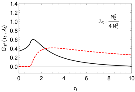
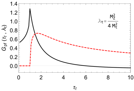
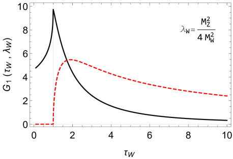
Figure 17: Behavior of the real (solid) and imaginary (dashed) parts of the form factors $G_{sf}(\tau_{t}\,,\lambda_{t})$ and $G_{pf}(\tau_{t}\,,\lambda_{t})$ (upper) and that of $G_{1}(\tau_{W}\,,\lambda_{W})$ (lower). We recall the relations $\tau_{x}=M_{H}^{2}/4M_{x}^{2}$ and $\lambda_{x}=M_{Z}^{2}/4M_{x}^{2}$. The vertical lines at $\tau_{x}=1$ denote the mass threshold above which $M_{H}>2M_{x}$.

The amplitude for the decay process $H\to Z\gamma$ can be written as [227]

$${\cal M}_{Z\gamma H}=-\,\frac{\alpha}{2\pi v}\Bigg{\{}S^{Z\gamma}(M_{H},M_{Z})\,\left[k_{1}\cdot k_{2}\,\epsilon_{1}^{*}\cdot\epsilon_{2}^{*}-k_{1}\cdot\epsilon_{2}^{*}\,k_{2}\cdot\epsilon_{1}^{*}\right]-P^{Z\gamma}(M_{H},M_{Z})\,\langle\epsilon_{1}^{*}\epsilon_{2}^{*}k_{1}k_{2}\rangle\Bigg{\}}\,,$$ (192)

with the two form factors of $S^{Z\gamma}$ and $P^{Z\gamma}$. Here $k_{1,2}$ are the momenta of the $Z$ boson and the photon (we note that $2k_{1}\cdot k_{2}=M_{H}^{2}-M_{Z}^{2}$), $\epsilon_{1,2}$ are their polarization vectors, and $\langle\epsilon_{1}\epsilon_{2}k_{1}k_{2}\rangle\equiv\epsilon_{\mu\nu\alpha\beta}\epsilon_{1}^{\mu}\epsilon_{2}^{\nu}k_{1}^{\alpha}k_{2}^{\beta}$. Retaining only the dominant contributions from third–generation fermions and $W^{\pm}$ and introducing two residual form factors $\Delta S^{Z\gamma}$ and $\Delta P^{Z\gamma}$ to parameterize contributions from the triangle loops in which non-SM particles are running, the scalar and pseudoscalar form factors are given by

$$S^{Z\gamma}(M_{H},M_{Z})\, = 2\sum_{f=t,b,\tau}N_{C}^{f}Q_{f}\frac{I_{3}^{f}-2s_{W}^{2}Q_{f}}{s_{W}c_{W}}\ g^{S}_{H\bar{f}f}\ G_{sf}(\tau_{f},\lambda_{f})-\frac{1}{s_{W}}\,g_{{}_{HWW}}G_{1}(\tau_{W},\lambda_{W})+\Delta S^{Z\gamma}\,,$$

$$P^{Z\gamma}(M_{H},M_{Z})\, = 2\sum_{f=t,b,\tau}N_{C}^{f}Q_{f}\frac{I_{3}^{f}-2s_{W}^{2}Q_{f}}{s_{W}c_{W}}\ g^{P}_{H\bar{f}f}\ G_{pf}(\tau_{f},\lambda_{f})+\Delta P^{Z\gamma}\,,$$ (193)

where $I_{3}^{\,u,\nu}=+1/2$, $I_{3}^{\,d,e}=-1/2$, $\tau_{x}=M_{H}^{2}/4m_{x}^{2}$ and $\lambda_{x}=M_{Z}^{2}/4m_{x}^{2}$, respectively. The loop functions are given by:

$$G_{sf}(\tau_{f},\lambda_{f}) = I_{2}(\tau_{f},\lambda_{f})-I_{1}(\tau_{f},\lambda_{f})\,;\ \ \ G_{pf}(\tau_{f},\lambda_{f})=I_{2}(\tau_{f},\lambda_{f})\,,$$ (194)

$$G_{1}(\tau_{W},\lambda_{W}) = c_{W}\ \Bigg{\{}\left[2\tau_{W}(t_{W}^{2}-1)+(t_{W}^{2}-5)\right]I_{1}(\tau_{W},\lambda_{W})+4(3-t_{W}^{2})I_{2}(\tau_{W},\lambda_{W})\Bigg{\}}\,,$$

where $I_{1,2}$ are functions of the two variables of $\tau$ and $\lambda$ and they are expressed as

$$I_{1}(\tau,\lambda) = \frac{1}{2(\lambda-\tau)}+\frac{1}{2(\lambda-\tau)^{2}}\left[f(\tau)-f(\lambda)\right]+\frac{\lambda}{(\lambda-\tau)^{2}}\left[g(\tau)-g(\lambda)\right]\,,$$

$$I_{2}(\tau,\lambda) = -\frac{1}{2(\lambda-\tau)}\left[f(\tau)-f(\lambda)\right]\,,$$ (195)

in terms of the $f(\tau)$ function, defined in Eq. (175), and the function $g(\tau)$ which is defined as

$$g(\tau)=\left\{\begin{array}[]{cl}\sqrt{\frac{1}{\tau}-1}\,{\rm arcsin}(\sqrt{\tau})\,:&\qquad\tau\leq 1\,,\\[5.69054pt] \frac{1}{2}\sqrt{\frac{\tau-1}{\tau}}\left[\ln\left(\frac{\sqrt{\tau}+\sqrt{\tau-1}}{\sqrt{\tau}-\sqrt{\tau-1}}\right)-i\pi\right]\,:&\qquad\tau\geq 1\,.\end{array}\right.$$ (198)

The explicit $\tau_{x}$ dependence of the form factors $G_{sf}$ and $G_{pf}$ for $x=t$ and $G_{1}$ for $x=W$ is shown in Fig. 17, clearly exhibiting the development of their imaginary parts beyond $M_{H}>2M_{x}$ with $\lambda_{t,W}<1$.

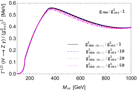
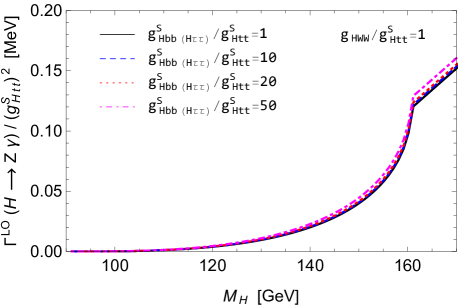
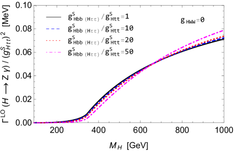
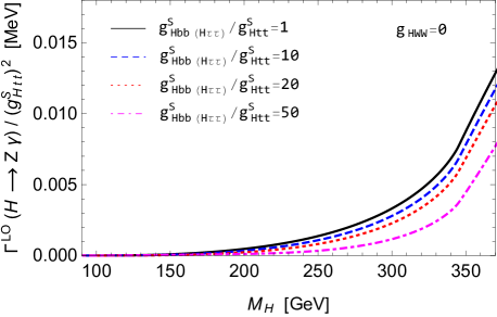
Figure 18: (Upper) Normalized decay widths of a neutral Higgs boson with a mass $M_{H}$ into $Z\gamma$ at LO taking $g_{{}_{HWW}}/g^{S}_{H\bar{t}t}=1$ and $g^{P}_{H\bar{f}f}=\Delta S^{Z\gamma}=\Delta P^{Z\gamma}=0$ for four values of $g^{S}_{H\bar{b}b\,,H\tau\tau}/g^{S}_{H\bar{t}t}=1\,,10\,,20$, and $50$. In the right panel, the low $M_{H}$ region is magnified. (Lower) The same as in the upper panels but taking $g_{{}_{HWW}}=0$.

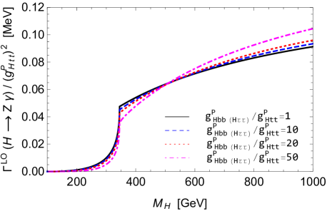
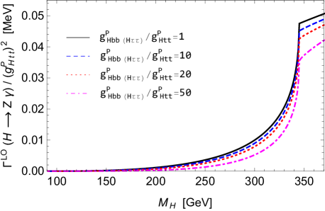
Figure 19: Normalized decay widths of a neutral Higgs boson with a mass $M_{H}$ into $Z\gamma$ via the pseudoscalar form factor $P^{Z\gamma}$ at LO taking $\Delta P^{Z\gamma}=0$. In this case, only the fermion couplings of $g^{P}_{H\bar{f}f}$ with $f=t,b,\tau$ are relevant.

At LO, the radiative decay width is given by [228, 229, 230]

$$\Gamma^{\rm LO}(H\to Z\gamma)\,=\,\frac{\alpha(0)\,G_{F}^{2}M_{W}^{2}s_{W}^{2}}{64\pi^{4}}M_{H}^{3}\left(1-\frac{M_{Z}^{2}}{M_{H}^{2}}\right)^{3}\,\left(\left|S^{Z\gamma}(M_{H},M_{Z})\right|^{2}+\left|P^{Z\gamma}(M_{H},M_{Z})\right|^{2}\right)\,.$$ (199)

A detailed description of the scalar and pseudoscalar form factors in the framework of the MSSM taken as a specific BSM model is given in Appendix B.

The QCD corrections turn out to be less than $0.3$% [231, 232, 233]. On the other hand, the theoretical uncertainties of the electroweak corrections have been estimated as $\sim 5$% [84] which constitutes the largest theoretical uncertainty involved in the experimentally clean and/or dominant SM Higgs decay modes into $b\bar{b}\,,WW\,,gg\,,\tau\tau\,,c\bar{c}\,,ZZ\,,\gamma\gamma\,,Z\gamma$ , and $\mu\mu$.

Experimentally, the $H\to Z\gamma$ mode has to be extracted from the Dalitz decays of $H\to\gamma f\bar{f}$ [234, 235, 236, 237, 238, 239, 240] which consist of: $(i)$ the $H\to Z^{(*)}\gamma$ decay followed by the decay $Z^{(*)}\to f\bar{f}$, $(ii)$ the tree-level process $H\to f\bar{f}$ with a photon radiated from the final-state fermions, $(iii)$ the loop-induced process $H\to\gamma\gamma^{*}$ via triangle diagrams followed by the decay $\gamma^{*}\to f\bar{f}$, $(iv)$ the loop-induced process $H\to\gamma f\bar{f}$ via box diagrams and $(v)$ the loop-induced process $H\to f\bar{f}$ via triangle diagrams with a photon radiated from the final-state fermions. For a clean separation of the $H\to Z\gamma$ decay from other processes, appropriate experimental cuts have to be imposed.

In the upper panels of Fig. 18, we show the LO decay width into a vector boson $Z$ and a photon normalized to the $g_{H\bar{t}t}$ coupling squared taking $g_{{}_{HWW}}/g^{S}_{H\bar{t}t}=1$ and $g^{P}_{H\bar{f}f}=\Delta S^{Z\gamma}=\Delta P^{Z\gamma}=0$ for the four values of $g^{S}_{H\bar{b}b\,,H\tau\tau}/g^{S}_{H\bar{t}t}=1,\,10,\,20$, and $50$. This reduces to the SM decay width of a Higgs particle weighing $M_{H}$ when $g_{{}_{HWW}}/g^{S}_{H\bar{t}t}=g^{S}_{H\bar{b}b\,,H\tau\tau}/g^{S}_{H\bar{t}t}=1$ together with $g_{H\bar{t}t}=1$. Below the $W$-boson-pair threshold, the $W$-loop contributions are dominant, leading to the sharp rise as $M_{H}$ approaches $2M_{W}$. Passing the $W$-pair threshold $M_{H}=2M_{W}$ from below, the real part of the $W$-loop contributions decreases while the imaginary part starts to develop leading to another mild rise, see the lower panel of Fig. 17. Passing $M_{H}=2M_{t}$, the $t$-quark loop contributions start to cancel that of the $W$-loop contributions as shown in the upper-left panel of Fig. 18. In the lower panels, we show the results taking $g_{{}_{HWW}}=0$ for the four values of $g^{S}_{H\bar{b}b\,,H\tau\tau}/g^{S}_{H\bar{t}t}=1\,,10\,,20\,,50$. This case may apply to the heavy neutral Higgs bosons appearing in the 2HDMs and/or MSSM when their couplings to the massive vector bosons are suppressed and they are almost vanishing [225, 226].

In Fig. 19, the alternative pseudoscalar choice is made to show $\Gamma(H\to Z\gamma)/(g^{P}_{H\bar{t}t})^{2}$ taking the four values of $g^{P}_{H\bar{b}b}/g^{P}_{H\bar{t}t}=g^{P}_{H\tau\tau}/g^{P}_{H\bar{t}t}=1\,,10\,,20\,,50$ with $\Delta S^{Z\gamma}=\Delta P^{Z\gamma}=0$. Here we assume all the scalar couplings of $g^{S}_{H\bar{f}f}$ are vanishing. Note that, in this case, only the fermion loops are contributing as the pseudoscalar state does not couple to gauge bosons at the tree level. In the right panel, as the same as in Fig. 18, we magnify the low $M_{H}$ regions. Compared to the scalar case shown in Fig. 18, it is clearly shown in Fig. 19 that the scalar and pseudoscalar decays exhibit quite distinct patterns, in particular, around the $t$-pair threshold. The distinct patterns between the scalar case with $g_{{}_{HWW}}=0$ (two lower frames of Fig. 18) and the pseudoscalar one (Fig. 19) basically come from the differences in sizes and behaviors of the form factors $G_{sf}$ and $G_{pf}$ shown in Fig. 17.

Table 4: The leading $M_{H}$ dependence and the ballpark values of normalized decay widths of the neutral Higgs boson $H$ far above the mass threshold of its decay products. Specifically, we have taken $M_{H}=1$ TeV. For the radiative loop-induced decays, the scalar (upper) and pseudoscalar (lower) contributions are shown separately. For the scalar contributions to $H\to\gamma\gamma$ and $H\to Z\gamma$ which are dominated by $t$-quark and $W$-boson loops, we assume $g^{S}_{H\bar{t}t}=g_{{}_{HWW}}=1$. See Table 12 for the $\overline{\rm MS}$ quark masses $\overline{m}_{q}(M_{H})$ while we refer to Eq. (A.5) for $m_{q}(\mu=M_{H}/2)$.

Decay Mode	Leading $M_{H}$ dependence	$\Gamma_{M_{H}=1\rm{TeV}}^{\rm\,normalized}$ [GeV]	Reference Figure
$H\rightarrow f\bar{f}$	$M_{H}$	$40\left[\frac{\overline{m}_{q}(M_{H})}{\overline{m}_{t}(M_{H})}\right]^{2}$	Figs. 1 and 2
		$\frac{40}{3}\left[\frac{M_{\tau\,,\mu}}{\overline{m}_{t}(M_{H})}\right]^{2}$
$H\rightarrow WW\,(ZZ)$	$M_{H}^{3}$	$350\,(180)$	Fig. 6
$H\rightarrow\varphi V$	$M_{H}^{3}$	$300$	Fig. 7
$H\rightarrow\varphi\varphi$	$1/M_{H}$	$4$
$H\rightarrow gg$	$M_{H}^{3}\left|F_{sf}\left(\frac{M_{H}^{2}}{4M_{t}^{2}}\right)\right|^{2}$	$7\times 10^{-2}$	Fig. 10
	$M_{H}^{3}\left|F_{pf}\left(\frac{M_{H}^{2}}{4M_{t}^{2}}\right)\right|^{2}$	$9\times 10^{-2}$	Fig. 11
$H\rightarrow\gamma\gamma$	$M_{H}^{3}\left|\frac{8}{3}F_{sf}\left(\frac{M_{H}^{2}}{[4m_{t}(M_{H}/2)]^{2}}\right)-F_{1}\left(\frac{M_{H}^{2}}{4M_{W}^{2}}\right)\right|^{2}$	$3\times 10^{-4}$	Fig. 15
	$M_{H}^{3}\left|F_{pf}\left(\frac{M_{H}^{2}}{[4m_{t}(M_{H}/2)]^{2}}\right)\right|^{2}$	$3\times 10^{-4}$	Fig. 16
$H\rightarrow Z\gamma$	$M_{H}^{3}\left|0.9\,G_{sf}\left(\frac{M_{H}^{2}}{4M_{t}^{2}},\frac{M_{Z}^{2}}{4M_{t}^{2}}\right)-G_{1}\left(\frac{M_{H}^{2}}{4M_{W}^{2}},\frac{M_{Z}^{2}}{4M_{W}^{2}}\right)\right|^{2}$	$6\times 10^{-4}$	Fig. 18
	$M_{H}^{3}\left|G_{pf}\left(\frac{M_{H}^{2}}{4M_{t}^{2}},\frac{M_{Z}^{2}}{4M_{t}^{2}}\right)\right|^{2}$	$8\times 10^{-5}$	Fig. 19

Table 5:  The QCD and ELW corrections to the decay widths of neutral and charged Higgs bosons which are denoted by $H$ and $H^{+}$, respectively. The abbreviations used are: NC $=$ Not Considered, [S] $=$ Scalar part, [P] $=$ Pseudoscalar part.

Decay Mode	Expressions for a partial width	QCD corrections	ELW corrections
$H\to b\bar{b}\,,c\bar{c}$	Eq. (145)	Eq. (3.1)
$H\to\tau^{+}\tau^{-}\,,\mu^{+}\mu^{-}$	Eq. (145)	$-\!\!\!-\!\!\!-$	$\begin{array}[]{c}{\rm[S]}\,:\,{\rm Eq}.~{}(\ref{eq:ghff_elw})\\[5.69054pt] {\rm[P]}\,:\,{\rm NC}\end{array}$
$H\to t\bar{t}$	$\begin{array}[]{c}{\rm Eq}.~{}(\ref{eq:ghtt})\,{\rm for}\,M_{H}\leq 500~{}{\rm GeV}\\[-8.53581pt] {\rm Eq}.~{}(\ref{eq:ghff})\,{\rm for}\,M_{H}>500~{}{\rm GeV}\end{array}$	Eq. (3.1)
$H\to WW\,,ZZ$	Eqs. (160,163)	$-\!\!\!-\!\!\!-$	Fig. 5 (PROPHECY4Fv3.0)
$H\to\varphi Z$	Eq. (165)
$H\to\varphi^{\pm}W^{\mp}$	Eq. (167)	$-\!\!\!-\!\!\!-$	NC
$H\to\varphi\varphi$	Eq. (169)
$H\to gg$	Eq. (176)	$\begin{array}[]{c}{\rm[S]}\,:\,{\rm Eq}.~{}(\ref{eq:ghgg_qcd_s})\\[-8.53581pt] {\rm[P]}\,:\,{\rm Eq}.~{}(\ref{eq:ghgg_qcd_p})\end{array}$	$\begin{array}[]{c}{\rm[S]}\,:\,{\rm Fig}.~{}\ref{fig:gSelw}~{}({\rm Grids})\\[-8.53581pt] {\rm[P]}\,:\,{\rm Eq}.~{}(\ref{eq:ghgg_elw_p}){}{}{}{}{}{}\end{array}$
$H\to\gamma\gamma$	Eqs. (184,190)	Eq. (184) $\oplus$ Eq. (3.5)	$\begin{array}[]{c}{\rm[S]}\,:\,{\rm Fig}.~{}\ref{fig:dhaaelw}~{}({\rm Grids})\\[-8.53581pt] {\rm[P]}\,:\,{\rm Eq}.~{}(\ref{eq:dhaaelwP}){}{}{}{}{}{}{}\end{array}$
$H\to Z\gamma$	Eq. (199)	$-\!\!\!-\!\!\!-$	NC
$H^{+}\to c\bar{s}$	Eq. (228)	$\delta_{\rm QCD}$ in Eq. (3.1)
$H^{+}\to\nu\tau^{+}\,,\nu\mu^{+}$	Eq. (228)	$-\!\!\!-\!\!\!-$	NC
$H^{+}\to t\bar{b}$	$\begin{array}[]{c}{\rm Eq}.~{}(\ref{eq:gchtb})\,{\rm for}\,M_{H^{\pm}}\leq 500~{}{\rm GeV}\\[-8.53581pt] {\rm Eq}.~{}(\ref{eq:gchff})\,{\rm for}\,M_{H^{\pm}}>500~{}{\rm GeV}\end{array}$	$\delta_{\rm QCD}$ in Eq. (3.1)
$H^{+}\to HW^{+}$	Eq. (229)	$-\!\!\!-\!\!\!-$	NC

Before moving to the last subsection for numerical results obtained by analyzing the decays of several neutral Higgs bosons, we provide Table 4 in which the leading $M_{H}$ dependence and the ballpark values of normalized decay widths at $M_{H}=1$ TeV are shown for all the decay modes elaborated on up to this subsection. Table 5 is further provided for a summary of the QCD and electroweak corrections considered in Section 3 and Section 4 which are for the decays of $H$ and $H^{+}$, respectively.

3.7 Numerical results

Closing this section dedicated to a detailed study of neutral Higgs boson decays, we present the results of two numerical analyses of $(i)$ the decays of a neutral Higgs boson with its mass fixed to $125.5$ GeV dictated by the LHC discovery and $(ii)$ the decays of heavy neutral Higgs bosons which are mixtures of CP-even and CP-odd states.

In the first numerical analysis, we extend the SM in a somewhat model-independent way by allowing for the pseudoscalar as well as scalar couplings of the $125.5$ GeV Higgs boson and perform a comprehensive analysis of its decays by estimating all the widths and branching ratios as precise as possible. For the second numerical analysis, we have specifically chosen the type-I 2HDM in which the Yukawa couplings of the lightest Higgs boson as well as its couplings to a pair of massive vector bosons quickly approach the corresponding SM values as the masses of the heavy neutral Higgs bosons increase and their decouplings are not delayed [242, 243, 244]. In this model, there is no much need of decoupling the heavy Higgs bosons to avoid conflicts with the current LHC Higgs precision data. Moreover, though assuming that the lightest neutral Higgs boson is a purely CP-even state, the heavy neutral states could still undergo a significant CP-violating mixing in the presence of CP-violating phases in the Higgs potential [245, 246, 247].

We emphasize that the numerical analyses performed in this subsection are solely based on the detailed analytical and numerical results presented in this Section 3 and supplemental materials provided in Appendices.

3.7.1 Anatomy of Higgs boson decays with $M_{H}=125.5$ GeV

In this subsubsection, we present all the details of calculating the decay widths of a neutral Higgs boson by taking $M_{H}=125.5$ GeV [10], while allowing for nontrivial pseudoscalar as well as scalar couplings of the Higgs boson to fermion pairs. The SM parameters taken in this present analysis are summarized in Appendix A. Note that one may apply the results to the genuine CP-even SM Higgs boson by taking $g^{S}_{H\bar{f}f}=g_{{}_{HVV}}=1$ and $g^{P}_{H\bar{f}f}=\Delta S^{g\,,\gamma\,,Z\gamma}=\Delta P^{g\,,\gamma\,,Z\gamma}=0$.

For the decays of a neutral Higgs boson with $M_{H}=125.5$ GeV into $b$ and $c$ quarks and muons and tau leptons, the relevant radiative corrections are given numerically by

$$\delta_{\rm QCD} = +0.203+0.037+0.002-0.001=+0.241\,;$$

$$\delta^{b:S}_{t} = +0.011\,\xi^{b:S}_{t}\,,\ \ \delta^{c:S}_{t}\ \ \ =+0.019\,\xi^{c:S}_{t};$$

$$\delta^{b}_{\rm elw} = -0.005\,,\ \ \delta^{c}_{\rm elw}\ \ \ =+0.004\,;\ \ \delta^{\tau}_{\rm elw}=-0.0097\,,\ \ \delta^{\mu}_{\rm elw}=-0.0307\,;$$

$$\delta^{b}_{\rm mixed} = -0.001\,,\ \ \delta^{c}_{\rm mixed}=-0.000\,;$$

$$\delta^{b}_{\rm tot} = +0.244\,,\ \ \delta^{c}_{\rm tot}\ \ \ =+0.265\,;\ \ \delta^{\tau}_{\rm tot}\,=-0.0097\,,\ \ \delta^{\mu}_{\rm tot}\,=-0.0307\,,$$ (200)

with the rescaling factors defined by $\xi^{q:S(P)}_{t}\equiv g_{H\bar{t}t}^{S(P)}/g_{H\bar{q}q}^{S(P)}$. Incidentally, we have $\delta^{b:P}_{t}=0.018\,\xi^{b:P}_{t}$ and $\delta^{c:P}_{t}=0.030\,\xi^{c:P}_{t}$ contributing to the pseudoscalar part.

For the decays $H\to WW,ZZ$, from Fig. 5, we have two electroweak corrections as

$$\delta^{W}_{\rm elw}=0.0308\,,\ \ \ \delta^{Z}_{\rm elw}=0.0152\,.$$ (201)

For the decay $H\to gg$, the scalar and pseudoscalar form factors and the relevant radiative corrections are given numerically apart from the scalar and pseudoscalar Higgs–fermion–fermion couplings by

$$S^{g} = 0.688\,g_{H\bar{t}t}^{S}+(-0.043+0.062\,i)\,g_{H\bar{b}b}^{S}+(-0.009+0.008\,i)\,g_{H\bar{c}c}^{S}+\Delta S^{g}\,;$$

$$P^{g} = 1.048\,g_{H\bar{t}t}^{P}+(-0.049+0.063\,i)\,g_{H\bar{b}b}^{P}+(-0.010+0.008\,i)\,g_{H\bar{c}c}^{P}+\Delta P^{g}\,;$$

$$\delta^{g:S}_{\rm QCD} = 0.8850\,,\ \ \delta^{g:S}_{\rm elw}=0.0516\,;\ \ \delta^{g:P}_{\rm QCD}=0.8775\,,\ \ \delta^{g:P}_{\rm elw}=-0.0218\,,$$ (202)

where $\delta^{g:S}_{\rm elw}$ is from Fig. 9 and we set $\eta^{g:P}_{\rm elw}=0$ for $\delta^{g:P}_{\rm elw}$. In the SM, we have $S^{g}=0.636+0.070\,i$ and $P^{g}=0$. Similarly for the decay $H\to\gamma\gamma$, in terms of the $HWW$ and Higgs–fermion–fermion couplings, we obtain the following scalar and pseudoscalar form factors

$$S^{\gamma} = -8.341\,g_{{}_{HWW}}+1.826\,g_{H\bar{t}t}^{S}+(-0.020+0.024\,i)\,g_{H\bar{b}b}^{S}+(-0.023+0.021\,i)\,g_{H\tau\tau}^{S}+\Delta S^{\gamma}\,;$$

$$P^{\gamma} = 2.772\,g_{H\bar{t}t}^{P}+(-0.022+0.024\,i)\,g_{H\bar{b}b}^{P}+(-0.025+0.021\,i)\,g_{H\tau\tau}^{P}+\Delta P^{\gamma}\,;$$

$$\delta^{\gamma:S}_{\rm QCD} = 0.016\,,\ \ \delta^{\gamma:S}_{\rm elw}=-0.016\,;\ \ \delta^{\gamma:P}_{\rm QCD}=0.028\,,\ \ \delta^{\gamma:P}_{\rm elw}=-0.012\,,$$ (203)

where the QCD corrections are obtained by implementing the scaling factors $C_{sf,pf}(\tau_{t,b})$ into the form factors $F_{sf,pf}(\tau_{t,b})$ and the electroweak correction $\delta^{\gamma:S}_{\rm elw}$ is from Fig. 13. For $\delta^{\gamma:P}_{\rm elw}$, we set $\eta^{\gamma:P}_{\rm elw}=0$. For the numerical estimate of $\delta^{\gamma:S}_{\rm QCD}$, more precisely, we take the SM values of $g_{{}_{HWW}}=g^{S}_{H\bar{t}t}=g^{S}_{H\bar{b}b}=g^{S}_{H\tau\tau}=1$. While, for the numerical estimate of $\delta^{\gamma:P}_{\rm QCD}$, we assume a scenario in which the pseudoscalar form factor $P^{\gamma}$ is dominated by the top-quark contribution taking $g^{P}_{H\bar{b}b}=g^{P}_{H\tau\tau}=0$, i.e. neglecting the $b$– and $\tau$–loop contributions. In the SM, we have $S^{\gamma}=-6.558+0.047\,i$ and $P^{\gamma}=0$.

Finally, for the decay $H\to Z\gamma$, the scalar and pseudoscalar form factors are given by

$$S^{Z\gamma} = -12.372\,g_{{}_{HWW}}+0.689\,g_{H\bar{t}t}^{S}+(-0.019+0.011\,i)\,g_{H\bar{b}b}^{S}+(-0.0005+0.0002\,i)\,g_{H\tau\tau}^{S}+\Delta S^{Z\gamma}\,;$$

$$P^{Z\gamma} = 1.046\,g_{H\bar{t}t}^{P}+(-0.022+0.011\,i)\,g_{H\bar{b}b}^{P}+(-0.0006+0.0002\,i)\,g_{H\tau\tau}^{P}+\Delta P^{Z\gamma}\,,$$ (204)

in terms of the $HWW$ and Higgs–fermion–fermion couplings. In the SM, we have $S^{Z\gamma}=-11.702+0.011\,i$ and $P^{Z\gamma}=0$. The $H\to Z\gamma$ decay width is estimated at LO.

Table 6: Partial and total decay widths of the SM Higgs in MeV taking $M_{H}=125.5$ GeV. We compare our numerical estimates with those presented in Ref. [84] by introducing a quantity $\delta_{\Gamma}$ defined by $\delta_{\Gamma}\equiv\left(\Gamma_{\rm This~{}Review}-\Gamma_{\rm Ref.\small{\cite[cite]{[\@@bibref{}{deFlorian:2016spz}{}{}]}}}\right)/\Gamma_{\rm Ref.\small{\cite[cite]{[\@@bibref{}{deFlorian:2016spz}{}{}]}}}$. Also presented are theoretical uncertainties (THUs) of the partial and total decay widths from missing higher orders estimated around $M_{H}=125$ GeV, see Tables 178 and 182 in Ref. [84].

	$\Gamma(H\rightarrow b\bar{b})$	$\Gamma(H\to WW)$	$\Gamma(H\to gg)$	$\Gamma(H\to\tau\tau)$	$\Gamma(H\to c\bar{c})$
This Review	$2.367$	$9.185\times 10^{-1}$	$3.382\times 10^{-1}$	$2.572\times 10^{-1}$	$1.173\times 10^{-1}$
Ref. [84]	$2.387$	$9.222\times 10^{-1}$	$3.386\times 10^{-1}$	$2.573\times 10^{-1}$	$1.185\times 10^{-1}$
$\delta_{\Gamma}$ [%]	$-0.8$	$-0.4$	$-0.1$	$-0.05$	$-1.0$
THU [%]	$\pm 0.5$	$\pm 0.5$	$\pm 3.2$	$\pm 0.5$	$\pm 0.5$
	$\Gamma(H\to ZZ)$	$\Gamma(H\to\gamma\gamma)$	$\Gamma(H\to Z\gamma)$	$\Gamma(H\to\mu\mu)$	$\Gamma_{\rm tot}$
This Review	$1.139\times 10^{-1}$	$9.405\times 10^{-3}$	$6.531\times 10^{-3}$	$8.913\times 10^{-4}$	$4.129$
Ref. [84]	$1.139\times 10^{-1}$	$9.438\times 10^{-3}$	$6.550\times 10^{-3}$	$8.927\times 10^{-4}$	$4.156$
$\delta_{\Gamma}$ [%]	$-0.03$	$-0.4$	$-0.3$	$-0.2$	$-0.65$
THU [%]	$\pm 0.5$	$\pm 1.0$	$\pm 5.0$	$\pm 0.5$	$\pm 0.73$

In Table  6, we show the partial and total decay widths of the SM Higgs boson with $M_{H}=125.5$ GeV taking $g^{S}_{H\bar{f}f}=g_{{}_{HVV}}=1$ and $g^{P}_{H\bar{f}f}=\Delta S^{g\,,\gamma\,,Z\gamma}=\Delta P^{g\,,\gamma\,,Z\gamma}=0$. For a quantitative comparison with those presented in Ref. [84], we introduce $\delta_{\Gamma}$’s, which are defined by $\delta_{\Gamma}\equiv\left(\Gamma_{\rm This~{}Review}-\Gamma_{\rm Ref.\small{\cite[cite]{[\@@bibref{}{deFlorian:2016spz}{}{}]}}}\right)/\Gamma_{\rm Ref.\small{\cite[cite]{[\@@bibref{}{deFlorian:2016spz}{}{}]}}}$ for each decay mode, for being contrasted with theoretical uncertainties (THUs) given in Ref. [84]. In terms of $\delta_{\Gamma}/{\rm THU}$, we find excellent agreement between our analysis and that in Ref. [84] except for $H\to b\bar{b}$ and $H\to c\bar{c}$ for which we find $\delta_{\Gamma}/|{\rm THU}|\simeq-2$. The largest contribution to the discrepancy of $\Gamma_{\rm tot}$ comes from $H\to b\bar{b}$ with the second (third) largest one from $H\to WW\,(c\bar{c})$. We note that our estimations of the decay widths into quarks are smaller than those in Ref. [84]. This might come from our incomplete and rough implementation of the ELW corrections of Eq. (147).

Table 7: Branching ratios (BRs) of the SM Higgs taking $M_{H}=125.5$ GeV. We compare our numerical estimates with those presented in Ref. [84]. Estimation of the total uncertainty THU$+$PU has been done by adding linearly the THU and the total parametric uncertainty (PU) where the latter is obtained by adding the individual PUs in quadrature, see Tables 174, 175, 176, 177, and 178 in Ref. [84].

	${B}(H\rightarrow b\bar{b})$	${B}(H\to WW)$	${B}(H\to gg)$	${B}(H\to\tau\tau)$	${B}(H\to c\bar{c})$
This Review	$5.733\times 10^{-1}$	$2.225\times 10^{-1}$	$8.190\times 10^{-2}$	$6.230\times 10^{-2}$	$2.841\times 10^{-2}$
Ref. [84]	$5.744\times 10^{-1}$	$2.219\times 10^{-1}$	$8.147\times 10^{-2}$	$6.192\times 10^{-2}$	$2.852\times 10^{-2}$
THU$+$PU [%]	$1.7$	$2.1$	$7.2$	$2.3$	$6.6$
	${B}(H\to ZZ)$	${B}(H\to\gamma\gamma)$	${B}(H\to Z\gamma)$	${B}(H\to\mu\mu)$	$\Gamma_{\rm tot}$[MeV]
This Review	$2.758\times 10^{-2}$	$2.278\times 10^{-3}$	$1.582\times 10^{-3}$	$2.159\times 10^{-4}$	$4.129$
Ref. [84]	$2.741\times 10^{-2}$	$2.271\times 10^{-3}$	$1.576\times 10^{-3}$	$2.148\times 10^{-4}$	$4.156$
THU$+$PU [%]	$2.1$	$2.9$	$6.9$	$2.4$	$1.9$

In Table 7, we show the branching ratios and the total decay width of the SM Higgs boson taking $M_{H}=125.5$ GeV. Again comparisons are made with those in Ref. [84] together with the total uncertainties. We pick up THUs and PUs from Tables 174, 175, 176, 177, and 178 in Ref. [84]. We note that the total uncertainty is about 2 - 3 % for $H\to b\bar{b},WW,\tau\tau,ZZ,\gamma\gamma$ and $\mu\mu$. While it is about 7 % for $H\to gg,c\bar{c}$, and $Z\gamma$. The total decay width is determined with about 2% error. In Fig. 20, the branching ratios (BRs) are shown in the Higgs-boson mass range between 120 GeV and 130 GeV. For each BR line, the band width represents the corresponding total uncertainty.

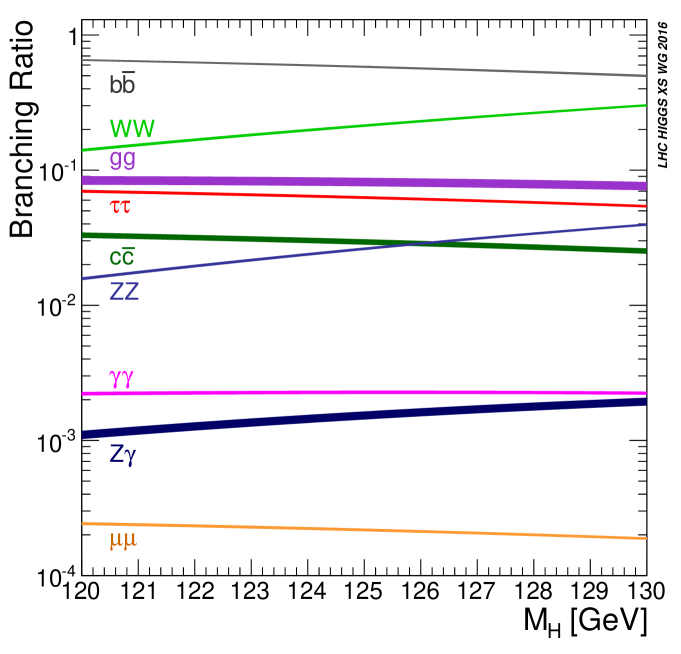
Figure 20: Higgs boson branching ratios and their uncertainties for the mass range around $125$ GeV. The plot is taken from Ref. [84].

3.7.2 Decays of heavy Higgs bosons in CP-violating 2HDMs

In this subsubsection, we study the decays of heavy neutral Higgs bosons appearing in BSM models. To be specific, we choose the type-I 2HDM identifying the lightest neutral Higgs boson as the SM-like $125.5$ GeV one discovered at the LHC. We assume that the lightest Higgs boson is purely CP even while the two heavier Higgs bosons exhibit nontrivial CP-violating (CPV) mixing in the presence of the complex quartic couplings of $\lambda_{5,6,7}$ in the Higgs potential. In this scenario, with no much need of decoupling the heavier Higgs bosons, all the branching ratios and the total decay width of the lightest Higgs boson remain consistent with those of the SM Higgs within the ranges allowed by the current LHC Higgs precision data [244]. The decay widths and branching ratios are calculated as summarized in Table 5 but the ELW corrections are neglected for consistency. For the full model- and parameter-dependent ELW corrections in 2HDMs, see Appendix F.

To fix all the relevant couplings of three neutral Higgs bosons, one may start from the orthogonal $3\times 3$ matrix $O$ describing the mixing among them. For CPV scenarios in 2HDMs, the three neutral Higgs bosons do not carry definite CP parities and they become mixtures of CP-even and CP-odd states. In this case, without loss of generality, the mixing matrix can be parameterized as

$$\vspace{ 1.0cm}O = \left(\begin{array}[]{ccc}-s_{\alpha}&c_{\alpha}&0\\ c_{\alpha}&s_{\alpha}&0\\ 0&0&1\\ \end{array}\right)\left(\begin{array}[]{ccc}c_{\eta}&0&s_{\eta}\\ 0&1&0\\ -s_{\eta}&0&c_{\eta}\\ \end{array}\right)\left(\begin{array}[]{ccc}1&0&0\\ 0&c_{\omega}&s_{\omega}\\ 0&-s_{\omega}&c_{\omega}\\ \end{array}\right)$$ (214)

$$= \left(\begin{array}[]{ccc}-s_{\alpha}c_{\eta}&c_{\alpha}c_{\omega}+s_{\alpha}s_{\eta}s_{\omega}&c_{\alpha}s_{\omega}-s_{\alpha}s_{\eta}c_{\omega}\\ c_{\alpha}c_{\eta}&s_{\alpha}c_{\omega}-c_{\alpha}s_{\eta}s_{\omega}&s_{\alpha}s_{\omega}+c_{\alpha}s_{\eta}c_{\omega}\\ -s_{\eta}&-c_{\eta}s_{\omega}&c_{\eta}c_{\omega}\\ \end{array}\right)\,,$$ (218)

introducing a CP-conserving (CPC) mixing angle $\alpha$ and two CPV angles $\omega$ and $\eta$. We recall that the mixing matrix $O$ relates the electroweak eigenstates $(\phi_{1}\,,\phi_{2}\,,a)$ to the mass eigenstates $(H_{1}\,,H_{2}\,,H_{3})$ via

$$(\phi_{1}\,,\phi_{2}\,,a)^{T}_{\alpha}=O_{\alpha i}(H_{1}\,,H_{2}\,,H_{3})^{T}_{i}\,,$$

with the ordering of $M_{H_{1}}\leq M_{H_{2}}\leq M_{H_{3}}$. Assuming the lightest Higgs boson is purely CP even or taking $s_{\eta}=0$ and $c_{\eta}=1$, the mixing matrix takes the simpler form of

$$\left.O\right|_{s_{\eta}=0,c_{\eta}=1}\ =\ \left(\begin{array}[]{ccc}-s_{\alpha}&c_{\alpha}c_{\omega}&c_{\alpha}s_{\omega}\\ ~{}~{}c_{\alpha}&s_{\alpha}c_{\omega}&s_{\alpha}s_{\omega}\\ ~{}0&-s_{\omega}&c_{\omega}\\ \end{array}\right)\,.$$ (219)

Note that, in the CP-conserving case, one of the heavy Higgs boson is purely CP odd and its coupling to a pair of massive gauges bosons is identically vanishing. We observe that $H_{3}$ is purely CP odd when $|c_{\omega}|=1$ while $H_{2}$ is CP odd when $|s_{\omega}|=1$. Plugging the above expression of $O$ into Eq. (2.3.2), the couplings of three neutral Higgs bosons to a pair of massive vector bosons are given by

$$g_{{}_{H_{1}VV}}=s_{\beta-\alpha}\equiv\sqrt{1-\epsilon}\,,\ \ \ g_{{}_{H_{2}VV}}=c_{\beta-\alpha}c_{\omega}\equiv\delta_{2}\,,\ \ \ g_{{}_{H_{3}VV}}=c_{\beta-\alpha}s_{\omega}\equiv\delta_{3}\,,$$ (220)

with $\delta_{2}^{2}+\delta_{3}^{2}=\epsilon$. We note that the two mixing angles are determined as follows

$$s_{\alpha} = -\sqrt{1-\epsilon}\,c_{\beta}+\frac{\delta_{2}}{c_{\omega}}\,s_{\beta}\,,\ \ \ c_{\alpha}=\sqrt{1-\epsilon}\,s_{\beta}+\frac{\delta_{2}}{c_{\omega}}\,c_{\beta}\,,$$

$$c_{\omega}^{2} = \frac{\delta_{2}^{2}}{\delta_{2}^{2}+\delta_{3}^{2}}=\frac{\delta_{2}^{2}}{\epsilon}\,,\ \ \ s_{\omega}^{2}=\frac{\delta_{3}^{2}}{\delta_{2}^{2}+\delta_{3}^{2}}=\frac{\delta_{3}^{2}}{\epsilon}\,.$$ (221)

in terms of the couplings $\delta_{2}=g_{{}_{H_{2}VV}}$ and $\delta_{3}=g_{{}_{H_{3}VV}}$ together with $t_{\beta}$. And then, the Yukawa couplings of the three neutral Higgs bosons are determined by

$$g^{S}_{H_{i}\bar{u}u}=g^{S}_{H_{i}\bar{d}d}=g^{S}_{H_{i}\bar{\ell}\ell}=O_{\phi_{2}i}/s_{\beta}\,;\ \ \ -g^{P}_{H_{i}\bar{u}u}=g^{P}_{H_{i}\bar{d}d}=g^{P}_{H_{i}\bar{\ell}\ell}=O_{ai}/t_{\beta}\,,$$ (222)

where $u$ and $d$ stand for the up- and down-type quarks, respectively, and $\ell$ for three charged leptons. To summarize, in the scenario under consideration, all the Yukawa couplings of the two heavy Higgs bosons could be fixed by giving their couplings to the massive vector bosons. On the other hand, depending on ${\rm sign}[\delta_{2}/c_{\omega}]$, all the Yukawa couplings of the lightest Higgs boson are determined by $O_{\phi_{2}1}/s_{\beta}=c_{\alpha}/s_{\beta}=\sqrt{1-\epsilon}\pm\sqrt{\epsilon}/t_{\beta}$ which, especially for large $t_{\beta}$, approaches the SM value of $1$ as quickly as the $g_{{}_{H_{1}VV}}=\sqrt{1-\epsilon}$ coupling when $\epsilon$ goes to zero. This is the very reason we choose the type-I 2HDM for our numerical study avoiding conflicts with the current LHC Higgs precision data [244].

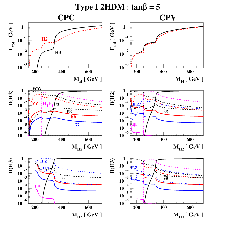
Figure 21: The total decay widths and branching ratios of the two heavy Higgs bosons in the type-I 2HDM taking $t_{\beta}=5$ and $|g_{{}_{H_{2}H_{1}H_{1}}}|=|g_{{}_{H_{3}H_{1}H_{1}}}|=0.1$. In the left CPC panels, we take $\delta_{2}^{2}=g_{{}_{H_{2}VV}}^{2}=2\epsilon_{0}\,(M_{H_{1}}^{4}/M_{H_{2}}^{4})=\epsilon$ and $\delta_{3}^{2}=g_{{}_{H_{3}VV}}^{2}=0$. While, in the right CPV panels, we take $\delta_{2}^{2}=g_{{}_{H_{2}VV}}^{2}=\epsilon_{0}\,(M_{H_{1}}^{4}/M_{H_{2}}^{4})$ and $\delta_{3}^{2}=g_{{}_{H_{3}VV}}^{3}=\epsilon_{0}\,(M_{H_{1}}^{4}/M_{H_{3}}^{4})$. In the both CPC and CPV cases, we take $\epsilon_{0}=0.05$.

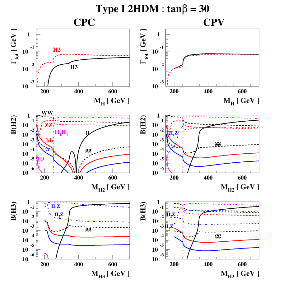
Figure 22: The same as in Fig. 21 but for $t_{\beta}=30$.

For our numerical study, we vary $t_{\beta}$ but, for $\delta_{2,3}$, we are taking

$$g_{{}_{H_{2}VV}}=\delta_{2}=\sqrt{\epsilon}_{0}\,\left(\frac{M_{H_{1}}}{M_{H_{2}}}\right)^{2}\,,\ \ \ g_{{}_{H_{3}VV}}=\delta_{3}=\sqrt{\epsilon}_{0}\,\left(\frac{M_{H_{1}}}{M_{H_{3}}}\right)^{2}\,,$$ (223)

reflecting the behavior of $\epsilon$ which is suppressed by the quartic powers of the heavy Higgs-boson masses at leading order [244]. With the above parameterizations of $\delta_{2,3}$ and taking $c_{\omega}>0$ we have $\delta_{2}/c_{\omega}=c_{\beta-\alpha}=\sqrt{\epsilon}>0$ and $s_{\omega}^{2}=M_{H_{2}}^{4}/(M_{H_{2}}^{4}+M_{H_{3}}^{4})$ leading to a maximal CPV mixing between the two heavy Higgs bosons when they are degenerate. For $\epsilon_{0}$ or the largest possible value of $\delta_{2,3}^{2}$, we choose a value which is a little bit larger than the lower $1\sigma$ error of $C_{v}$ in the CPC4 fit:

$$\epsilon_{0}=0.05\,,$$ (224)

having in mind the relation $g_{{}_{H_{1}VV}}=\sqrt{1-\epsilon}\geq\sqrt{1-2\epsilon_{0}}\simeq 1-\epsilon_{0}$. For the masses of Higgs bosons, we take

$$M_{H_{1}}=125.5\ {\rm GeV}\,,\ \ \ M_{H_{2}}=M_{H_{3}}-50\ {\rm GeV}\,,\ \ \ M_{H_{3}}<M_{H^{\pm}}\sim 1~{}{\rm TeV}\,,$$ (225)

with $M_{H_{3}}$ varied. This choice may result in the simpler decay pattern by forbidding or suppressing the decay channels of $H_{2,3}\to H^{\pm}W^{\mp*}$, $H_{2,3}\to H^{\pm}H^{\mp}$, $H_{3}\to H_{1}H_{2}$, $H_{3}\to H_{2}H_{2}$, etc. By assuming very heavy charged Higgs boson, also neglected are the contributions from the charged-Higgs-boson loops to the decay processes of the heavy neutral Higgs bosons into $\gamma\gamma$ and $Z\gamma$. Finally, for $H_{2,3}\to H_{1}H_{1}$, we take $|g_{{}_{H_{2}H_{1}H_{1}}}|=|g_{{}_{H_{3}H_{1}H_{1}}}|=0.1$. For the rigorous treatment of the cubic $H_{2}H_{1}H_{1}$ and $H_{3}H_{1}H_{1}$ self-couplings expressed in terms of the masses of charged and neutral Higgs bosons and the elements of the mixing matrix $O$, see Appendix E.

In Fig. 21, we show the decay widths and branching ratios of the two heavy Higgs bosons in the type-I 2HDM taking $t_{\beta}=5$. For CPC, $H_{3}$ is taken to be CP odd with $g_{{}_{H_{3}VV}}^{2}=0$ and, accordingly, the decays of $H_{3}$ into $WW$, $ZZ$, and $H_{1}H_{1}$ are forbidden. Incidentally, we note that $H_{2}\to H_{1}Z$ decay is also forbidden since $g_{{}_{H_{1}H_{2}Z}}^{2}=g_{{}_{H_{3}VV}}^{2}$. On the other hand, for CPV, there are no forbidden decay modes as long as they are kinematically allowed. In the CPC case, the total decay widths of CP-even $H_{2}$ and CP-odd $H_{3}$ are largely enhanced at the $H_{1}H_{1}$ and $t\bar{t}$ thresholds, respectively. While, in the CPV case, both of the thresholds contribute to the total decay widths as shown in the upper panels of Fig. 21.

For CPC, we further observe that the couplings of the CP-even state of $H_{2}$ to fermions are identically vanishing when $g^{S}_{H_{2}\bar{f}f}=0$. It does happen at $s_{\alpha}=0$ or $\epsilon=1/(1+t_{\beta}^{2})$, see Eq. (3.7.2). This explains why there are dips for the fermionic decay modes of the CP-even $H_{2}$ state at $M_{H_{2}}=[2\epsilon_{0}(1+t_{\beta}^{2})]^{1/4}M_{H_{1}}\simeq 70\,\sqrt{t_{\beta}}$ GeV as found in the middle-left panels of Fig. 21 and Fig. 22 around $M_{H_{2}}=160$ GeV and $385$ GeV, respectively. We note that the branching ratios of fermionic decay modes $H_{2,3}\to t\bar{t},b\bar{b},\tau\tau,\mu\mu$ are smaller for the larger value of $t_{\beta}$ since the corresponding decay widths are suppressed by the factor of $\sim 1/t_{\beta}^{2}$. For large values of $M_{H_{2,3}}$, the numerical results are consistent with the observation that the decay width of fermionic decay modes is proportional to $M_{H_{2,3}}$ while that of bosonic decay ones is inversely proportional to $M_{H_{2,3}}$ especially with the parameterization of Eq. (223) for $H_{2,3}\to VV\,,H_{1}Z$. On the other hand, the decay width $\Gamma(H_{3}\to H_{2}Z)$ is not suppressed by the heavy mass $M_{H_{3}}$ because of the relation $g_{{}_{H_{2}H_{3}Z}}^{2}=g_{{}_{H_{1}VV}}^{2}$. In our numerical study, it is suppressed since we have taken the small mass difference between $H_{3}$ and $H_{2}$ of $M_{H_{3}}-M_{H_{2}}=50\,{\rm GeV}<M_{Z}$. Otherwise, it may increase in proportion to $M_{H_{3}}^{3}$.

4 Decays of a Charged Higgs Boson

The effective couplings of the charged Higgs boson $H^{\pm}$ to quarks and leptons are described by the interaction Lagrangian:

$${\cal L}_{H^{\pm}f_{\uparrow}f_{\downarrow}}\ =\ \sqrt{2}\ H^{+}\,\overline{f_{\uparrow}}\,\left(\,\frac{m_{f_{\uparrow}}}{v}\,g_{f_{\uparrow}}\,P_{L}\ +\frac{m_{f_{\downarrow}}}{v}\,g_{f_{\downarrow}}\,P_{R}\,\right)\,{f_{\downarrow}}\ +\ {\rm h.c.}\,,$$ (226)

where $P_{L,R}=(1\mp\gamma_{5})/2$ and $({f_{\uparrow}},{f_{\downarrow}})=(t,b)\,,(c,s)\,,(\nu_{\tau},\tau)\,,(\nu_{\mu},\mu)$, etc. The masses of the up- and down-type fermions are denoted by $m_{f_{\uparrow}}$ and ${m}_{f_{\downarrow}}$, respectively. On the other hand, the interaction of the charged Higgs boson with a massive gauge boson $W$ and a neutral Higgs boson $H$ is given by

$${\cal L}_{HH^{\pm}W^{\mp}}=-\frac{g}{2}\,g_{{}_{HH^{+}W^{-}}}\,W^{-\mu}(H\,i\!\stackrel{{\scriptstyle\leftrightarrow}}{{\partial}}_{\mu}H^{+})\,+\,{\rm h.c.}\,,$$ (227)

with the convention $X\stackrel{{\scriptstyle\leftrightarrow}}{{\partial}}_{\mu}Y\equiv X(\partial_{\mu}Y)-(\partial_{\mu}X)Y$. With these effective interactions, in this section, we study the charged Higgs decays at LO except for the QCD corrections considered in the decay modes into quarks, concentrating on mainstream instead of being complete. For comprehensive studies of decays of a charged Higgs boson in BSM models, we refer to, for example, Refs. [248, 249, 250, 251].

When a charged Higgs boson decays into quarks, the decay width is given by

$$\Gamma(H^{+}\to{f_{\uparrow}}{f_{\downarrow}}) = N_{C}^{f_{\uparrow}f_{\downarrow}}\frac{M_{H^{\pm}}}{8\pi v^{2}}\lambda^{1/2}\left(1,\kappa_{f_{\uparrow}},\kappa_{f_{\downarrow}}\right)\,\Bigg{\{}\left(1-\kappa_{f_{\uparrow}}-\kappa_{f_{\downarrow}}\right)\left(m_{f_{\uparrow}}^{2}g_{f_{\uparrow}}^{2}+m_{f_{\downarrow}}^{2}g_{f_{\downarrow}}^{2}\right)$$ (228)

$$-4\sqrt{\kappa_{f_{\uparrow}}\kappa_{f_{\downarrow}}}\,m_{f_{\uparrow}}m_{f_{\downarrow}}g_{f_{\uparrow}}g_{f_{\downarrow}}\Bigg{\}}\,\left(1+\delta_{\rm QCD}\right)\,,$$

including the QCD correction factor $\delta_{\rm QCD}$ with $\kappa_{{f_{\uparrow}},{f_{\downarrow}}}=M^{2}_{{f_{\uparrow}},{f_{\downarrow}}}/M_{H^{\pm}}^{2}$ and $N_{C}^{f_{\uparrow}f_{\downarrow}}=3$. Note that the $\overline{\rm MS}$ quark masses such as $\overline{m}_{t,c}(M_{H^{\pm}})$ and $\overline{m}_{b,s}(M_{H^{\pm}})$ are taken for $m_{f_{\uparrow}}$ and $m_{f_{\downarrow}}$, respectively. While, for the decays into leptons, the charged lepton pole masses are used for $m_{f_{\downarrow}}$ together with $m_{f_{\uparrow}}=0$, $N_{C}^{f_{\uparrow}f_{\downarrow}}=1$, and $\delta_{\rm QCD}=0$. A charged Higgs boson may decay into a lighter neutral Higgs boson $H$ and a massive gauge boson $W$ and the LO decay width is given by [173, 166, 174]

$$\Gamma^{\rm LO}(H^{+}\rightarrow HW^{+*})=\frac{G_{F}M_{H^{\pm}}^{3}|g_{{}_{HH^{+}W^{-}}}|^{2}}{8\sqrt{2}\pi}\int_{0}^{(\sqrt{\omega_{\pm}}-\sqrt{\omega})^{2}}{\rm d}x\,\frac{\epsilon_{W}\lambda^{3/2}(\omega_{\pm},\omega,x)}{\omega_{\pm}^{3}\pi[(x-1)^{2}+\epsilon_{W}^{2}]}\,,$$ (229)

with $\omega=M_{H}^{2}/M_{W}^{2}$ and $\omega_{\pm}=M_{H^{\pm}}^{2}/M_{W}^{2}$. When $M_{H^{\pm}}$ is larger than the sum $M_{H}+M_{W}$, it reduces to

$$\Gamma^{\rm LO}(H^{+}\to HW^{+})\ =\ \frac{G_{F}M_{H^{\pm}}^{3}}{8\sqrt{2}\pi}|g_{{}_{HH^{+}W^{-}}}|^{2}\lambda^{3/2}(1,\kappa_{H},\kappa_{W})\,,$$ (230)

where $\kappa_{H}=M_{H}^{2}/M_{H^{\pm}}^{2}$ and $\kappa_{W}=M_{W}^{2}/M_{H^{\pm}}^{2}$. The electroweak corrections within the 2HDM framework have been calculated, specifically for the process of $H^{\pm}\to W^{\pm}h,W^{\pm}H,W^{\pm}A$ [252, 253, 254]. They are of moderate size and numerically stable if a process- and gauge-independent renormalization scheme is chosen [254]. Note that the package 2HDECAY [255] is available for the calculation of full ELW one-loop corrections to both neutral and charged Higgs decays in the CP-conserving 2HDM.

Finally, at LO, the decay widths of a charged Higgs boson $H^{+}$ into a chargino $\widetilde{\chi}_{j}^{+}$ and a neutralino $\widetilde{\chi}_{i}^{0}$ are given by

$$\Gamma^{\rm LO}(H^{+}\to\widetilde{\chi}_{j}^{+}\widetilde{\chi}_{i}^{0}) = \frac{g^{2}M_{H^{\pm}}\lambda^{1/2}(1,\kappa_{i},\kappa_{j})}{16\pi}$$

$$\times \left[(1\!-\!\kappa_{i}\!-\!\kappa_{j})(|g^{S}_{H^{+}\widetilde{\chi}_{i}^{0}\widetilde{\chi}_{j}^{-}}|^{2}+|g^{P}_{H^{+}\widetilde{\chi}_{i}^{0}\widetilde{\chi}_{j}^{-}}|^{2})-2\sqrt{\kappa_{i}\kappa_{j}}(|g^{S}_{H^{+}\widetilde{\chi}_{i}^{0}\widetilde{\chi}_{j}^{-}}|^{2}-|g^{P}_{H^{+}\widetilde{\chi}_{i}^{0}\widetilde{\chi}_{j}^{-}}|^{2})\right]\,,$$

with $\kappa_{i}=m_{\widetilde{\chi}_{i}^{0}}^{2}/M_{H^{\pm}}^{2}$ and $\kappa_{j}=m_{\widetilde{\chi}_{j}^{\pm}}^{2}/M_{H^{\pm}}^{2}$ and the LO decay widths into a pair of sfermions by

$$\Gamma^{\rm LO}(H^{+}\to\widetilde{f}_{i}\widetilde{f^{\prime}}_{j}^{*})=N_{C}^{ff^{\prime}}\frac{v^{2}\,|g_{H^{+}\widetilde{f}_{i}^{*}\widetilde{f^{\prime}}_{j}}|^{2}}{16\pi M_{H^{\pm}}}\lambda^{1/2}(1,\kappa_{i},\kappa_{j})\,,$$ (232)

where $\kappa_{i}=M_{\widetilde{f}_{i}}^{2}/M_{H^{\pm}}^{2}$, $\kappa_{j}=M_{\widetilde{f^{\prime}}_{j}}^{2}/M_{H^{\pm}}^{2}$, and $N_{C}^{ff^{\prime}}=3$ and $1$ for squarks and sleptons, respectively.

For a numerical example, we take the 2HDMs in which the relevant couplings are given by

$$H^{+}\to t\bar{b}\,,c\bar{s}\ : \ g_{f_{\uparrow}}=\frac{1}{t_{\beta}}\,,\ \ g_{f_{\downarrow}}=-\frac{1}{t_{\beta}}\,({\rm I\,,III})\,,\ t_{\beta}\,({\rm II\,,IV})\,;$$

$$H^{+}\to\nu\tau^{+}\,,\nu\mu^{+}\ : \ g_{f_{\uparrow}}=0\,,\ \ \ \,g_{f_{\downarrow}}=-\frac{1}{t_{\beta}}\,({\rm I\,,IV})\,,\ t_{\beta}\,({\rm II\,,III})\,;$$

$$H^{+}\to HW^{+}\ : \ |g_{{}_{HH^{+}W^{-}}}|^{2}=1-g_{{}_{HVV}}^{2}\,({\rm I\,,II\,,III\,,IV})\,,$$ (233)

depending on the 2HDM type as denoted by I, II, III or IV. For the decay $H^{+}\to HW^{+}$, we set $M_{H}=125.5$ GeV and $|g_{{}_{HH^{+}W^{-}}}|^{2}=0.1$. For the $\overline{\rm MS}$ mass of the strange quark, we take the approximation $\overline{m}_{s}(\mu)=\overline{m}_{c}(\mu)/11.72$ [6]. On the other hand, we neglect the effects of its pole mass which is relevant to the $H^{+}\to c\bar{s}$ decay only through the kinematical factor $\kappa_{s}$, see Eq. (228), and too tiny to influence the numerical results.

For the charged Higgs–boson decay $H^{+}\to t\bar{b}$, we take the contribution of the off-shell top quark into account [166, 174]:

$$\Gamma^{\rm LO}(H^{\pm}\to t(p_{t})\,\bar{b}\to b\bar{b}W^{+}) = N_{C}^{tb}\,\frac{1}{v^{2}}\frac{g^{2}M_{H^{\pm}}}{2^{9}\pi^{3}}\,\int_{M_{W}^{2}}^{(M_{H^{\pm}}-M_{b})^{2}}\,\lambda_{H^{\pm}}^{1/2}\,p_{t}^{2}\left(1-\frac{M_{W}^{2}}{p_{t}^{2}}\right)^{2}\left(2+\frac{p_{t}^{2}}{M_{W}^{2}}\right)$$ (234)

$$\times\,\frac{\left(1-\alpha_{t}-\alpha_{\bar{b}}\right)\left[\overline{m}_{t}^{2}(M_{H^{\pm}})g_{t}^{2}+\overline{m}_{b}^{2}(M_{H^{\pm}})g_{b}^{2}\right]-4\sqrt{\alpha_{t}\alpha_{\bar{b}}}\,\overline{m}_{t}(M_{H^{\pm}})\overline{m}_{b}(M_{H^{\pm}})g_{t}g_{b}}{(p_{t}^{2}-M_{t}^{2})^{2}+M_{t}^{2}\Gamma_{t}^{2}}\,dp_{t}^{2}\,,$$

where the kinematical $b$-quark mass is neglected in the $t\to bW^{+}$ decay process and the triangle function $\lambda_{H^{\pm}}$ is given by

$$\lambda_{H^{\pm}}=1+\alpha_{t}^{2}+\alpha_{\bar{b}}^{2}-2\alpha_{t}-2\alpha_{\bar{b}}-2\alpha_{t}\alpha_{\bar{b}}\,,$$ (235)

with $\alpha_{t}=p_{t}^{2}/M_{H^{\pm}}^{2}$ and $\alpha_{\bar{b}}=M_{b}^{2}/M_{H^{\pm}}^{2}$. When $M_{H^{\pm}}>M_{t}+M_{b}$, using Eqs. (155) and (157), we have

$$\Gamma^{\rm LO}(H^{\pm}\to t\,\bar{b}\to b\bar{b}W^{+})=\Gamma^{\rm LO}(H^{\pm}\to t\,\bar{b})\,\frac{\Gamma^{\rm LO}(t\to bW)}{\Gamma_{t}}\,,$$ (236)

in a factorized form.

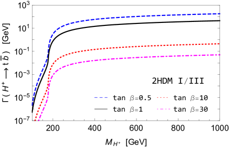
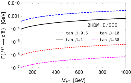
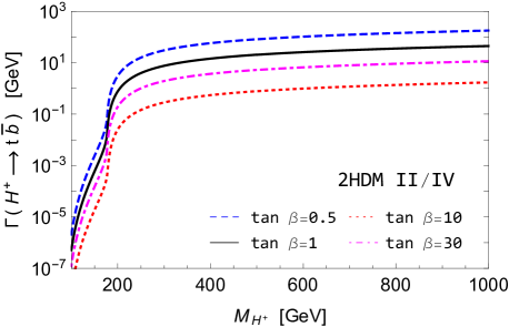
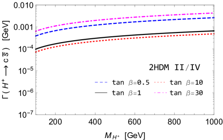
Figure 23: (Upper) Decay widths of a charged Higgs boson with a mass $M_{H^{\pm}}$ into $t\bar{b}$ (left) and $c\bar{s}$ (right) in the type-I and type-III 2HDMs. QCD corrections are taken into account. For $\tan\beta$, we take four values of $0.5$ (blue dashed), $1$ (black solid), $10$ (red dotted), and $30$ (magenta dash-dotted). (Lower) The same as in the upper panels but in the type-II and type-IV 2HDMs.

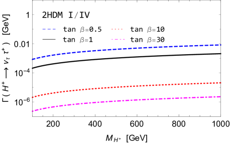
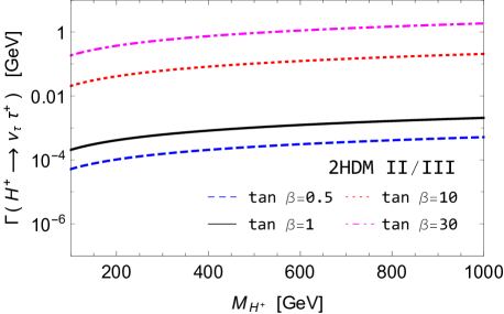
Figure 24: (Upper) Decay widths of a charged Higgs boson with a mass $M_{H^{\pm}}$ into $\tau^{+}\nu$ in the type-I/IV 2HDMs (left) and in the type-II/III ones (right). For $\tan\beta$, we take four values of $0.5$ (blue dashed), $1$ (black solid), $10$ (red dotted), and $30$ (magenta dash-dotted).

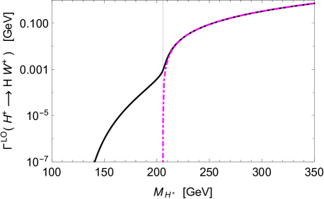
Figure 25: Decay widths of a charged Higgs boson with a mass $M_{H^{\pm}}$ into $HW^{+}$ taking $M_{H}=125.5$ GeV and $|g_{{}_{HH^{+}W^{-}}}|^{2}=0.1$. In the right panel, we magnify the low $M_{H}$ region and compare with the two-body decay width (dash-dotted magenta line). The vertical line locates the position $M_{H^{\pm}}=M_{H}+M_{W}$.

In the upper panels of Fig. 23, we show the decay widths of a charged Higgs boson into two quarks, $t^{(*)}\bar{b}$ (left) and $c\bar{s}$ (right) in the type-I and type-III 2HDMs taking account of the QCD corrections. In these models, $g_{t,c}=-g_{b,s}=1/t_{\beta}$ and the top-quark and charm-quark contributions dominate and the decay widths scale as $1/t_{\beta}^{2}$. In the lower panels of Fig. 23, we consider the type-II and type-IV 2HDMs in which $g_{t,c}=1/t_{\beta}$ and $g_{b,s}=t_{\beta}$. For low values of $t_{\beta}$, the top-quark and charm-quark contributions dominate and the decay widths scale as $1/t_{\beta}^{2}$. On the other hand, for high values of $t_{\beta}$, the bottom-quark and strange-quark contributions are enhanced by the factor of $t_{\beta}^{2}$ while the top-quark and charm-quark contributions are suppressed by the factor of $1/t_{\beta}^{2}$. The bottom-quark and strange-quark contributions start to dominate when $t_{\beta}$ is larger than $\sqrt{\overline{m}_{t}/\overline{m}_{b}}\simeq 7.7$ and $\sqrt{\overline{m}_{c}/\overline{m}_{s}}\simeq 3.4$, respectively. When the bottom-quark and strange-quark contributions dominate, the decay widths scale as $(t_{\beta}/60)^{2}$ and $(t_{\beta}/12)^{2}$, respectively, compared to the case with $t_{\beta}=1$ and these factors are responsible for the significant change of the decay widths for high $t_{\beta}$ values, as can be checked by comparing the lines with $t_{\beta}=1$ and those with $t_{\beta}=10$ and $30$.

In Fig. 24, we show the LO decay widths of a charged Higgs boson with mass $M_{H^{\pm}}$ into $\tau^{+}\nu$ in the type-I/IV 2HDMs (left) and in the type-II/III ones (right) taking $t_{\beta}=0.5$ (blue dashed), $1$ (black solid), $10$ (red dotted), and $30$ (magenta dash-dotted). In the type-I/IV and type-II/III 2HDMs, the decay widths scale as $g^{2}_{\tau}=1/t^{2}_{\beta}$ and $t^{2}_{\beta}$, respectively. Compared to the case of $H^{+}\to\tau^{+}\nu$, the decay widths $\Gamma(H^{+}\to\mu^{+}\nu)$ are simply suppressed by the large factor of $m_{\tau}^{2}/m_{\mu}^{2}\sim 300$.

In Fig. 25, we show the LO decay widths of a charged Higgs boson with a mass $M_{H^{\pm}}$ into $HW^{+}$ taking $M_{H}=125.5$ GeV and $|g_{{}_{HH^{+}W^{-}}}|^{2}=0.1$. In the right panel, we magnify the low $M_{H}$ region covering the case with a virtual $W^{+*}$ and we compare the decay width with the prediction of the two-body decay width (dash-dotted magenta line). We note that they are nearly identical for $M_{H^{\pm}}>M_{H}+M_{W}$, as expected.

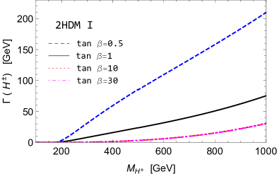
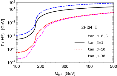
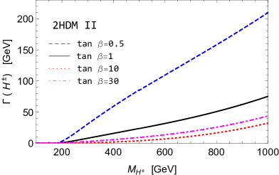
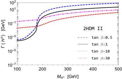
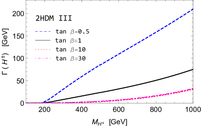
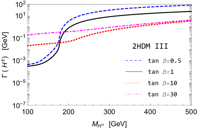
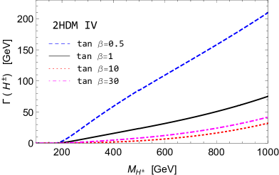
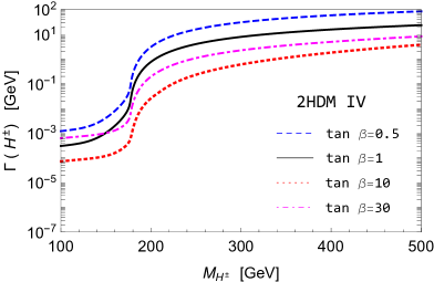
Figure 26: Total decay widths of a charged Higgs boson with a mass $M_{H^{\pm}}$ in the type-I, type-II, type-III, and type-IV 2HDMs from top to bottom. We are taking $\tan\beta=0.5$ (blue dashed), $1$ (black solid), $10$ (red dotted), and $30$ (magenta dash-dotted). In the right panels, we magnify the low $M_{H}$ region.

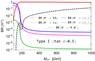
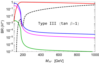
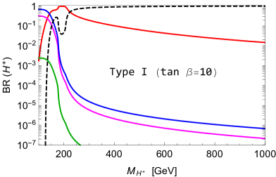
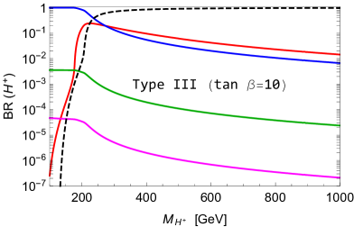
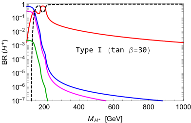
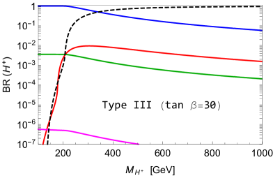
Figure 27: Branching ratios of a charged Higgs boson with a mass $M_{H^{\pm}}$ in the type-I (left) and type-III (right) 2HDMs taking $\tan\beta=0.5$, $1$, $10$, and $30$ from top to bottom. We consider 5 decay modes of $H^{+}\to t\bar{b}$ (red solid), $H^{+}\to c\bar{s}$ (magenta solid), $H^{+}\to\tau\nu$ (blue solid), $H^{+}\to\mu\nu$ (green solid), and $H^{+}\to HW^{+}$ (black dashed) with $M_{H}=125.5$ GeV and $|g_{{}_{HH^{+}W^{-}}}|^{2}=0.1$.

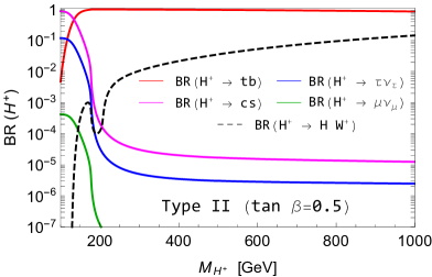
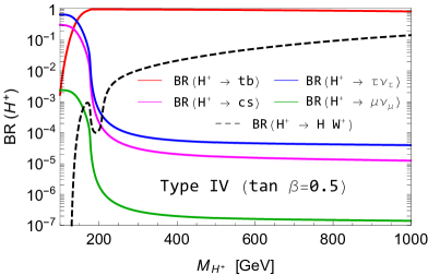
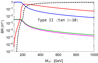
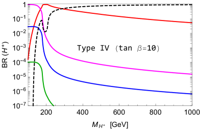
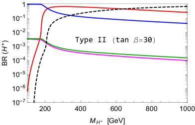
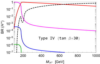
Figure 28: The same as in Fig. 27 but for the type-II (left) and type-IV (right) 2HDMs.

In Fig. 26, we show the total decay widths of a charged Higgs boson for four values of $t_{\beta}$: $\tan\beta=0.5$ (blue dashed), $1$ (black solid), $10$ (red dotted), and $30$ (magenta dash-dotted). We sum over the 5 decay modes of $H^{+}\to t\bar{b}$, $H^{+}\to c\bar{s}$, $H^{+}\to\tau\nu$, $H^{+}\to\mu\nu$, and $H^{+}\to HW^{+}$ with $M_{H}=125.5$ GeV and $|g_{{}_{HH^{+}W^{-}}}|^{2}=0.1$.

Firstly, we consider the total charged-Higgs decay width in the case of a heavy charged Higgs boson, see the left panels of Fig. 26. We note that the top-quark contributions to $\Gamma(H^{+}\to t\bar{b})$ scale as $1/t_{\beta}^{2}$, independently of the 2HDM types. As the value of $t_{\beta}$ grows, the total decay width monotonically decreases in the type-I and type-III 2HDMs. In contrast, in the type-II and type-IV 2HDMs, the decay width reaches the minimum around $t_{\beta}=8$, where the top-quark and bottom-quark contributions become comparable, and then it starts to increases as $t_{\beta}$ grows further. Based on these observations, we can work out the behavior of the total decay width of a heavy charged Higgs boson for large values of $t_{\beta}$: the dominant contribution comes from the $H^{+}\to HW^{+}$ decay mode with the subleading/competing contributions from $H^{+}\to t\bar{b}$. We identify that there exists an additional subleading contribution from $H^{+}\to\tau\nu$ for $t_{\beta}=10$ and $30$ in the type-II and type-III 2HDMs. On the other hand, for low values of $t_{\beta}$, the $H^{+}\to t\bar{b}$ decay mode dominates the total decay width with the subleading contribution from $H^{+}\to HW^{+}$ which amounts to about 30 GeV at $M_{H^{\pm}}=1$ TeV taking $M_{H}=125.5$ GeV and $|g_{{}_{HH^{+}W^{-}}}|^{2}=0.1$, see Fig. 25.

Secondly, we consider the case of a charged Higgs boson lighter than $t$ quark, see the right panels of Fig. 26. For large values of $t_{\beta}$, the $H^{+}\to\tau\nu$ decay mode dominates in the type-II and type-III 2HDMs. In the type-I 2HDM, the $H^{+}\to\tau\nu$ decay mode still dominates with the subleading contributions from $H^{+}\to c\bar{s}$ though both of them are suppressed by $1/t_{\beta}^{2}$. In the type-IV 2HDM, the $H^{+}\to c\bar{s}$ decay mode dominates where the strange-quark contribution is enhanced by $t_{\beta}^{2}$. For small values of $t_{\beta}$, the $H^{+}\to\tau\nu$ decay mode mostly dominates, leading to the larger decay widths for $t_{\beta}=0.5$ in the type-I and type-IV 2HDMs in which $|g_{\tau}|=1/t_{\beta}$.

In Fig. 27, we show the branching ratios of a charged Higgs boson varying its mass between 100 GeV and 1 TeV in the type-I and type-III 2HDMs taking $\tan\beta=0.5$, $1$, $10$, and $30$ from top to bottom. We consider 5 decay modes of $H^{+}\to t\bar{b}$ (red solid), $H^{+}\to c\bar{s}$ (magenta solid), $H^{+}\to\tau\nu$ (blue solid), $H^{+}\to\mu\nu$ (green solid), and $H^{+}\to HW^{+}$ (black dashed) with $M_{H}=125.5$ GeV. In the type-I and type-III models, the normalized charged Higgs couplings to quarks are the same because $g_{t,c}=|g_{b,s}|=1/t_{\beta}$ while those to leptons are given by $g_{\mu,\tau}=-1/t_{\beta}$ (type I) and $g_{\mu,\tau}=t_{\beta}$ (type III). We observe that, especially for large values of $t_{\beta}$, the heavy charged Higgs boson dominantly decays into $HW^{+}$ (black dashed) since $\Gamma(H^{+}\to t\bar{b})$ is suppressed as $t_{\beta}$ grows. And, when the $H^{+}\to HW^{+}$ decay mode dominates, the leptonic branching ratios are enhanced by $t_{\beta}^{2}$ in the type-III 2HDM. In the type-III 2HDM, we note that ${B}(H^{+}\to\tau\nu)$ becomes comparable to ${B}(H^{+}\to t\bar{b})$ around $t_{\beta}\sim 10$ and it becomes larger as $t_{\beta}$ grows.

In Fig. 28, we show the branching ratios of a charged Higgs boson for its mass between 100 GeV and 1 TeV in the type-II and type-IV 2HDMs taking $\tan\beta=0.5$, $1$, $10$, and $30$ from top to bottom. We consider the same 5 decay modes as in Fig. 27. In the type-II and type-IV models, the charged Higgs couplings to the (right-handed) up-type quarks are again given by $g_{t,c}=1/t_{\beta}$ but those to the down-type fermions are by $g_{b,s}=g_{\mu,\tau}=t_{\beta}$ (type II) and $g_{b,s}=1/|g_{\mu,\tau}|=t_{\beta}$ (type IV). We observe that, especially for large values of $t_{\beta}$, the heavy charged Higgs boson dominantly decays into $HW^{+}$ (black dashed) eventually. But, compared to the type-I and type-III 2HDMs where the top-quark contributions to the $H^{+}\to t\bar{b}$ decay always dominate and the decay width decreases as $t_{\beta}$ grows, the dominance of the $H^{+}\to HW^{+}$ decay mode develops rather slowly because the bottom-quark contributions take over the dominance around $t_{\beta}=8$ and the partial width $\Gamma(H^{+}\to t\bar{b})$ increases as $t_{\beta}$ grows in the type-II and type-IV 2HDMs. The leptonic decay widths are also enhanced by $t_{\beta}^{2}$ in the type-II 2HDM and we find that, specifically for $t_{\beta}=30$, the three decay modes of $H^{+}\to t\bar{b}$, $H^{+}\to HW^{+}$, and $H^{+}\to\tau\nu$ are competing in the region of $350\raisebox{-3.69899pt}{~{}\shortstack{$<$ \\ [-0.07cm] $\sim$}}~{}M_{H^{\pm}}/{\rm GeV}\raisebox{-3.69899pt}{~{}\shortstack{$<$ \\ [-0.07cm] $\sim$}}~{}600$.

For a light charged Higgs boson, it mostly decays into $\tau\nu$ and/or $c\bar{s}$ before the $H^{+}\to t^{*}\bar{b}$ decay channel opens and starts to dominate. Exceptions occur in the type-I and type-III 2HDMs when $t_{\beta}$ is large, see the lowest panels of Fig. 27. Specifically, for $t_{\beta}=30$ in the type-I model, the charged Higgs boson dominantly decays into $HW^{+*}$ in the narrow region of $M_{H^{\pm}}$ between 150 GeV and 180 GeV.

We confirm that the behavior of the branching ratio of each decay mode versus $M_{H^{\pm}}$ does not depend on the 2HDM type when $t_{\beta}=1$ as it should be: see the $\tan\beta=1$ panels in Figs. 27 and 28.

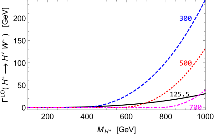
Figure 29: Decay widths of a charged Higgs boson with a mass $M_{H^{\pm}}$ into $H^{\prime}W^{+}$ for three values of $M_{H^{\prime}}=300$ GeV (blue dashed), $500$ GeV (red dotted), and $700$ GeV (magenta dash-dotted) taking $|g_{{}_{H^{\prime}H^{+}W^{-}}}|^{2}=1$. For comparisons, $\Gamma^{\rm LO}(H^{+}\to HW^{+})$ with $M_{H}=125.5$ GeV and $|g_{{}_{HH^{+}W^{-}}}|^{2}=0.1$ is also shown in black solid line, see Fig. 25.

Before closing this section, we address the case in which there exists another neutral Higgs boson $H^{\prime}$ with its mass smaller than $M_{H^{\pm}}$ and the decay $H^{+}\to H^{\prime}W^{+}$ is kinematically allowed. Here $H^{\prime}$ stands for a mixture of CP-even and CP-odd states in general which, in the CP-conserving case, could be either of them. In the 2HDM framework, identifying the lightest neutral Higgs boson as the SM-like $H$ with $M_{H}=125.5$ GeV and $|g_{{}_{HH^{+}W^{-}}}|^{2}=1-g_{{}_{HVV}}^{2}=0.1$ as already considered, the charged Higgs coupling to the heavier neutral Higgs boson $H^{\prime}$ and a charged vector boson $W$ takes almost the maximum value of $1$ due to the sum rules given in Eq. (54). Furthermore, the decay width grows by the cubic powers of the charged Higgs-boson mass. These combined properties result in a large width for the decay mode $H^{\pm}\to H^{\prime}W^{\pm}$ when ${H^{\pm}}$ is heavy enough. When $M_{H^{\pm}}\raisebox{-3.69899pt}{~{}\shortstack{$>$ \\ [-0.07cm] $\sim$}}~{}950$ GeV, we observe that the decay width $\Gamma^{\rm LO}(H^{+}\to H^{\prime}W^{+})$ is larger than 200 GeV for a $H^{\prime}$ boson with $M_{H^{\prime}}=300$ GeV, see the blue dashed line in Fig. 29. Even for $H^{\prime}$ as heavy as 700 GeV, we note that the decay width could be comparable to $\Gamma^{\rm LO}(H^{+}\to HW^{+})$ when $M_{H^{\pm}}\sim 1$ TeV as denoted by the magenta dash-dotted line in the same figure.

5 Higgcision of the Higgs Boson Discovered at the LHC

Ever since the discovery of a SM-like Higgs boson in the year 2012 [1, 2], the era of Higgs-boson precision studies, which was termed as Higgcision in Refs. [256, 257, 258], has begun. In this section we present highlights from global fits of the Higgs boson couplings to all the 7 TeV, 8 TeV, and 13 TeV data available up to the Summer 2018, based on the works [256, 257, 258]. For several different types of approaches with their own merits on the global fits of the Higgs couplings, see, for example, Refs. [84, 259, 260, 261, 262, 263, 264, 265, 266, 267, 268, 269, 270, 88, 271]. For some other early works based on model-independent approach, we refer to Refs. [272, 273, 274, 275, 276, 277, 278, 279, 280, 281, 282, 283, 284, 285, 286, 287, 288].

Assuming generation independence for the normalized Yukawa couplings of $g^{S,P}_{H\bar{f}f}$, we use the following $C$ notations for the couplings in the global fits:

$$C_{u}^{S}=g^{S}_{H\bar{u}u}\,,\ \ C_{d}^{S}=g^{S}_{H\bar{d}d}\,,\ \ C_{\ell}^{S}=g^{S}_{H\bar{l}l}\,;\ \ C_{w}=g_{{}_{HWW}}\,,\ \ C_{z}=g_{{}_{HZZ}}\,;$$

$$C_{u}^{P}=g^{P}_{H\bar{u}u}\,,\ \ C_{d}^{P}=g^{P}_{H\bar{d}d}\,,\ \ C_{\ell}^{P}=g^{P}_{H\bar{l}l}\,.$$ (237)

We further keep the custodial symmetry between the $W$ and $Z$ bosons which leads to the relation $C_{v}\equiv C_{w}=C_{z}$. We emphasize that one can carry out the precision study of the LHC Higgs data using the model-independent approach taken in Section 3 for decays of a generic neutral Higgs boson by matching the relevant couplings and fitting parameters as in Eq. (5).

5.1 Higgs signal strengths

Each theoretical signal strength can be written in a product form as

$$\widehat{\mu}({\cal P},{\cal D})\simeq\widehat{\mu}({\cal P})\ \widehat{\mu}({\cal D})\,,$$ (238)

where ${\cal P}={\rm ggF},{\rm VBF},{\rm VH},{\rm ttH}$ denote the production mechanisms and ${\cal D}=\gamma\gamma,ZZ^{(*)},WW^{(*)},b\bar{b},\tau^{+}\tau^{-}$ the decay channels, which are experimentally clean and/or dominant for $M_{H}\simeq 125\,{\rm GeV}$. The factorization assumption is valid only when the production and decay processes are well separated like as in the resonant $s$-channel Higgs production in the NWA. By factorizing them, non-resonant and interference effects are inevitably neglected. More explicitly, at LO, the production signal strengths are given in terms of the relevant form factors and couplings by

$$\widehat{\mu}({\rm ggF}) = \frac{\left|S^{g}(M_{H})\right|^{2}+\left|P^{g}(M_{H})\right|^{2}}{\left|S^{g}_{\rm SM}(M_{H})\right|^{2}}\,,$$

$$\widehat{\mu}({\rm VBF}) = \widehat{\mu}({\rm VH})=g_{{}_{HWW,HZZ}}^{2}\,,$$

$$\widehat{\mu}({\rm ttH}) = \left(g^{S}_{H\bar{t}t}\right)^{2}+\left(g^{P}_{H\bar{t}t}\right)^{2}\,,$$ (239)

and the decay signal strengths by

$$\widehat{\mu}({\cal D})=\frac{B(H\to{\cal D})}{B(H_{\rm SM}\to{\cal D})}\,,$$ (240)

with the branching fraction of each decay mode defined by

$$B(H\to{\cal D})=\frac{\Gamma(H\to{\cal D})}{\Gamma_{\rm tot}(H)+\Delta\Gamma_{\rm tot}}\,.$$ (241)

Note that an arbitrary non-SM contribution $\Delta\Gamma_{\rm tot}$ to the total decay width is introduced. We observe $\Gamma_{\rm tot}(H)$ becomes the SM total decay width when $g^{S}_{H\bar{f}f}=1$, $g^{P}_{H\bar{f}f}=0$, $g_{{}_{HWW,HZZ}}=1$, and $\Delta S^{\gamma,g,Z\gamma}=\Delta P^{\gamma,g,Z\gamma}=0$. Note that the LO relations in Eq. (5.1) are most reliable when higher order corrections to a BSM production cross section and those to the corresponding SM one are the same and so they are canceled out in the BSM-to-SM ratios. Otherwise they are valid at LO strictly.

Table 8: (Tevatron: 1.96 TeV) The signal strengths data from Tevatron (10.0 fb^-1 at 1.96 TeV).

Channel	Signal strength $\mu$	$M_{H}$(GeV)	Production mode				$\chi^{2}_{\rm SM}$(each)
	c.v $\pm$ error		ggF	VBF	VH	ttH
Tevatron (Nov. 2012)
Combined $H\to\gamma\gamma$[289]	$6.14^{+3.25}_{-3.19}$	125	78%	5%	17%	-	2.60
Combined $H\to WW^{(\ast)}$[289]	$0.85^{+0.88}_{-0.81}$	125	78%	5%	17%	-	0.03
VH tag $H\to bb$[290]	$1.59^{+0.69}_{-0.72}$	125	-	-	100%	-	0.67
							$\chi^{2}_{\rm SM}$(subtot): 3.30

Table 9: (LHC: 7$\oplus$8 TeV) Combined ATLAS and CMS data on signal strengths from Table 8 of Ref. [291].

	Decay mode
Production mode	$H\to\gamma\gamma$	$H\to ZZ^{(\ast)}$	$H\to WW^{(\ast)}$	$H\to bb$	$H\to\tau^{+}\tau^{-}$
ggF	$1.10^{+0.23}_{-0.22}$	$1.13^{+0.34}_{-0.31}$	$0.84^{+0.17}_{-0.17}$	-	$1.0^{+0.6}_{-0.6}$
VBF	$1.3^{+0.5}_{-0.5}$	$0.1^{+1.1}_{-0.6}$	$1.2^{+0.4}_{-0.4}$	-	$1.3^{+0.4}_{-0.4}$
WH	$0.5^{+1.3}_{-1.2}$	-	$1.6^{+1.2}_{-1.0}$	$1.0^{+0.5}_{-0.5}$	$-1.4^{+1.4}_{-1.4}$
ZH	$0.5^{+3.0}_{-2.5}$	-	$5.9^{+2.6}_{-2.2}$	$0.4^{+0.4}_{-0.4}$	$2.2^{+2.2}_{-1.8}$
ttH	$2.2^{+1.6}_{-1.3}$	-	$5.0^{+1.8}_{-1.7}$	$1.1^{+1.0}_{-1.0}$	$-1.9^{+3.7}_{-3.3}$
					$\chi^{2}_{\rm SM}$(subtot): 19.93

Table 10: (LHC: 13 TeV) Combined ATLAS and CMS (13 TeV) data on signal strengths. The $\mu^{\rm dec}_{\rm combined}$ ($\mu^{\rm prod}_{\rm combined}$) represents the combined signal strength for a specific decay (production) channel by summing all the production (decay) modes, and $\chi^{2}_{\rm min}$ are the corresponding minimal $\chi^{2}$ values. In the VH/WH row, the production mode for $H\to\gamma\gamma$ and $H\to ZZ^{(*)}$ is VH while it is WH for $H\to WW^{(*)}$ and $H\to\tau^{+}\tau^{-}$; for the remaining decay mode $H\to b\bar{b}$, we combine the two signal strengths from WH and VH, see Table XII in Ref. [258].

	Decay mode
Production mode	$H\to\gamma\gamma$	$H\to ZZ^{(\ast)}$	$H\to WW^{(\ast)}$	$H\to bb$	$H\to\tau^{+}\tau^{-}$	$\mu^{\rm prod}_{\rm combined}$	$\chi^{2}_{\rm SM}(\chi^{2}_{\rm min})$
ggF	$1.02^{+0.12}_{-0.11}$	$1.09^{+0.11}_{-0.11}$	$1.29^{+0.16}_{-0.16}$	$2.51^{+2.43}_{-2.01}$	$1.06^{+0.40}_{-0.37}$	$1.11^{+0.07}_{-0.07}$	5.42(3.15)
VBF	$1.23^{+0.32}_{-0.31}$	$1.51^{+0.59}_{-0.59}$	$0.54^{+0.32}_{-0.31}$	-	$1.15^{+0.36}_{-0.34}$	$1.02^{+0.18}_{-0.18}$	7.53(7.51)
VH/WH	$1.42^{+0.51}_{-0.51}$	$0.71^{+0.65}_{-0.65}$	$3.27^{+1.88}_{-1.70}$	$1.07^{+0.23}_{-0.22}$	$3.39^{+1.68}_{-1.54}$	$1.15^{+0.20}_{-0.19}$	7.05(6.44)
ZH	-	-	$1.00^{+1.57}_{-1.00}$	$1.20^{+0.33}_{-0.31}$	$1.23^{+1.62}_{-1.35}$	$1.19^{+0.32}_{-0.30}$	0.45(0.02)
ttH	$1.36^{+0.38}_{-0.37}$	$0.00^{+0.53}_{-0.00}$	-	$0.91^{+0.45}_{-0.43}$	-	$0.93^{+0.24}_{-0.24}$	5.96(5.86)
ttH (excl.)	$1.39^{+0.48}_{-0.42}$	-	$1.59^{+0.44}_{-0.43}$	$0.77^{+0.36}_{-0.35}$	$0.87^{+0.73}_{-0.73}$	$1.16^{+0.22}_{-0.22}$	4.17(3.62)
$\mu^{\rm dec}_{\rm combined}$	$1.10^{+0.10}_{-0.10}$	$1.05^{+0.11}_{-0.11}$	$1.20^{+0.14}_{-0.13}$	$1.05^{+0.19}_{-0.19}$	$1.15^{+0.24}_{-0.23}$	$1.10^{+0.06}_{-0.06}$
$\chi^{2}_{\rm SM}$($\chi^{2}_{\rm min}$)	6.83(5.72)	9.13(8.88)	9.48(7.32)	1.56(1.51)	3.58(3.20)		30.58(27.56)

On the experimental side, we use the direct Higgs signal strength data collected at the Tevatron and the LHC. Specifically, we use 3 signal strengths measured at the Tevatron, see Table 8. At the LHC with the center-of-mass energies of 7 and 8 (7$\oplus$8) TeV, the signal strengths obtained from a combined ATLAS and CMS analysis [291] are used, see Table 9. On the other hand, the 13 TeV data are still given separately by ATLAS and CMS and in different production and decay channels. Under this situation, to derive the combined signal strengths of various channels, we use a simple $\chi^{2}$ method assuming that each distribution is Gaussian. The results are shown in Table 10.

5.2 Constraints on the couplings of Higgs boson weighing $125.5$ GeV

In this subsection, we present a few representative results obtained from performing LO analysis of the direct Higgs data collected at the Tevatron and the LHC by considering CP-conserving (CPC) scenarios only. Note that, in the most general CPC scenario, one may vary all the 7 parameters of $C_{u}^{S}$, $C_{d}^{S}$, $C_{\ell}^{S}$,$C_{v}$, $\Delta S^{g}$, $\Delta S^{\gamma}$, and $\Delta\Gamma_{\rm tot}$ while taking vanishing pseudoscalar couplings and form factors as $C_{u}^{P}=C_{d}^{P}=C_{\ell}^{P}=\Delta P^{\gamma}=\Delta P^{g}=0$.

Table 11: (CPC) The best-fitted values in various CP conserving fits and the corresponding $\chi^{2}$ per degree of freedom (dof) and goodness of fit. The $p$-value for each fit hypothesis against the SM null hypothesis is also shown. For the SM, we obtain $\chi^{2}=53.81$, $\chi^{2}/dof=53.81/64$, and so the goodness of fit $=0.814$. From Ref. [258].

Cases	CPC1	CPC2	CPC4	CPCN4
Varying	$\Delta\Gamma_{\rm tot}$	$\Delta S^{\gamma}$	$C^{S}_{u},~{}C^{S}_{d},$	$C^{S}_{u},C_{v}$
Parameters		$\Delta S^{g}$	$C^{S}_{\ell},~{}C_{v}$	$\Delta S^{\gamma}$, $\Delta S^{g}$
$C^{S}_{u}$	1	1	$1.001^{+0.056}_{-0.055}$	$1.042^{+0.077}_{-0.081}$	$1.042^{+0.078}_{-0.081}$	$-1.042^{+0.081}_{-0.078}$	$-1.042^{+0.081}_{-0.078}$
$C^{S}_{d}$	1	1	$0.962^{+0.101}_{-0.101}$	$1$	$1$	$1$	$1$
$C^{S}_{\ell}$	1	1	$1.024^{+0.093}_{-0.093}$	$1$	$1$	$1$	$1$
$C_{v}$	1	1	$1.019^{+0.044}_{-0.045}$	$1.027^{+0.034}_{-0.036}$	$1.027^{+0.034}_{-0.036}$	$1.028^{+0.034}_{-0.036}$	$1.028^{+0.034}_{-0.036}$
$\Delta S^{\gamma}$	0	$-0.226^{+0.32}_{-0.32}$	0	$-0.129^{+0.37}_{-0.37}$	$-0.129^{+0.37}_{-0.37}$	$3.524^{+0.41}_{-0.42}$	$3.523^{+0.41}_{-0.42}$
$\Delta S^{g}$	0	$0.016^{+0.025}_{-0.025}$	0	$-0.021^{+0.057}_{-0.055}$	$-1.34^{+0.066}_{-0.065}$	$0.095^{+0.055}_{-0.057}$	$1.414^{+0.066}_{-0.066}$
$\Delta\Gamma_{\rm tot}$ (MeV)	$-0.285^{+0.18}_{-0.17}$	0	0	0	0	0	0
$\chi^{2}/dof$	51.44/63	51.87/62	50.79/60	50.96/60
goodness of fit	0.851	0.817	0.796	0.791
$p$-value	0.124	0.379	0.554	0.583

Our goal is to provide constraints on the couplings of the neutral Higgs boson, which was discovered at the LHC, without much loss of generality when it is interpreted in various frameworks beyond the SM. Accordingly, we consider the four CPC fits listed in Table 11 in which the second row explicitly shows the varying parameters of each fit.

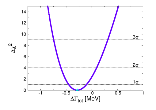
Figure 30: CPC1: $\Delta\chi^{2}$ from the minimum versus $\Delta\Gamma_{\rm tot}$ with only $\Delta\Gamma_{\rm tot}$ varying in the fit. From Ref. [258].

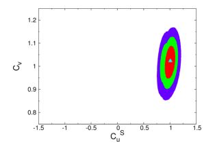
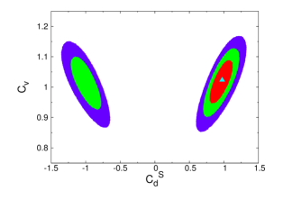
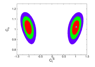
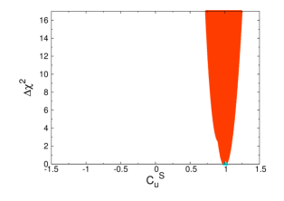
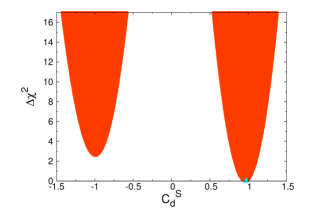
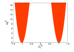
Figure 31: CPC4: (Upper) The confidence-level (CL) regions of the fit by varying $C_{v}$, $C_{u}^{S}$, $C_{d}^{S}$, and $C_{\ell}^{S}$. The contour regions shown are for $\Delta\chi^{2}\leq 2.3$ (red), $5.99$ (red+green), and $11.83$ (red+green+blue) above the minimum, which correspond to confidence levels of 68.3%, 95%, and 99.7%, respectively. The best-fit points are denoted by triangles. (Lower) $\Delta\chi^{2}$ from the minimum versus Yukawa couplings. From Ref. [258].

Referring to Ref. [258] for more detailed explanations, we offer highlights of each fit as follows:

1. CPC1: The best-fit value for the residual total decay width $\Delta\Gamma_{\rm tot}$ is $\Delta\Gamma_{\rm tot}=-0.285\,^{+0.18}_{-0.17}\;{\rm MeV}$ which is $1.6\,\sigma$ below zero. At 95% confidence level (CL), on the other hand,

   $$\Delta\Gamma_{\rm tot}=-0.285^{+0.38}_{-0.32}\ \ {\rm MeV}\,,$$ (242)

   as shown in Fig. 30. Using the upper error as the upper limit, we obtain the constraint $\Delta\Gamma_{\rm tot}\leq 0.38$ MeV simply taking the central value equal to zero which can be translated to the following 95% CL constraint on the branching ratio of the Higgs boson decays into non-SM particles: $B(H\to{\rm nonstandard})\leq 8.4\%$.

2. CPC2: The best-fit point $(\Delta S^{\gamma},\Delta S^{g})=(-0.226,0.016)$ of the form factors indicates an increase of 3.4% and 2.4% in the absolute values of the scalar $H\gamma\gamma$ and $Hgg$ form factors of $|S^{\gamma}|$ and $|S^{g}|$, respectively. We note that the error of $\Delta S^{g}$ is $\pm 0.025$, which is numerically smaller than the SM bottom-quark contribution of $-0.043$ to the real part of $S^{g}$, see Eq. (3.7.1), alerting that we have already reached the sensitivity to probe the sign of the bottom-quark Yukawa coupling in gluon fusion.

3. CPC4: We observe that the possibility for the top-quark Yukawa coupling to be negative has been entirely ruled out as shown clearly in the left upper and lower panels of Fig. 31. And, as already anticipated in the CPC2 fit, the bottom-quark Yukawa coupling $C_{d}^{S}$ prefers the positive sign to the negative one, see the middle panels of Fig. 31. It is more clear from the middle lower panel that the point $C_{d}^{S}=-1$ has $\Delta\chi^{2}>2$ above the minimum at $C_{d}^{S}=+1$. The current data precision is yet insufficient for showing any preference for the sign of tau-Yukawa coupling, as shown in the right panels of Fig. 31.

4. CPCN4: In this fit, there are 4 degenerate minima with $\Delta S^{g}\sim 0\,,\mp 1.4$ for $C_{u}^{S}\sim\pm 1$ which could be understood from the relation $|S^{g}|\sim|0.7\,C^{u}_{S}+\Delta S^{g}|\sim 0.7$, see Table 11. Note that $\Delta S^{\gamma}$ can compensate the sign change in $C_{u}^{S}$ allowing it to be about $-1$ with $\Delta S^{\gamma}\sim+3.5$. This could be understood by noting the relation $|S^{\gamma}|\sim|-8.3\,C_{v}+1.8\ C^{u}_{S}+\Delta S^{\gamma}|\sim 6.5$. We further observe that the negative top-quark Yukawa coupling is allowed only when there exist additional particles running in the $H$-$\gamma$-$\gamma$ loop with the size of contributions equal to two times the SM top-quark contribution within about 10 %. This tuning on the couplings and form factors will become more and more severe as more data are accumulated at the LHC.

5.3 Implications beyond the Standard Model

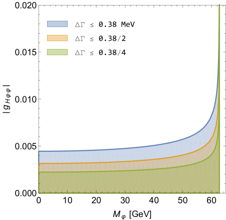
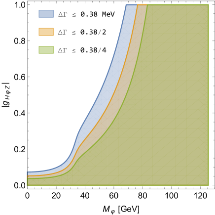
Figure 32: (Left) The allowed parameter space on the ($M_{\varphi}$, $|g_{H\varphi\varphi}|$) plane from $\Delta\Gamma_{\rm tot}\leq 0.38$ MeV at 95% CL. Also shown are future prospects assuming two and four times stronger constraints on $\Delta\Gamma_{\rm tot}$. (Right) The same as in the left panel but for ($M_{\varphi}$, $|g_{H\varphi Z}|$).

In the cxSM where the SM is extended by adding a complex SU(2)_L singlet, there could be a light Higgs boson $\varphi$ mainly from the singlet sector and the 125.5 GeV Higgs boson $H$ may couple to a pair of them through the singlet-doublet mixing term in the potential. When kinematically allowed or $2M_{\varphi}<125.5$ GeV, $H$ decays into a pair of light scalars and, in this case, $\Delta\Gamma_{\rm tot}\leq 0.38$ MeV may provide constraints on the mass $M_{\varphi}$ of the scalar particle and the absolute value of the coupling $g_{H\varphi\varphi}$ at 95% CL. We find $|g_{H\varphi\varphi}|\raisebox{-3.69899pt}{~{}\shortstack{$<$ \\ [-0.07cm] $\sim$}}~{}0.005$ for $M_{\varphi}\raisebox{-3.69899pt}{~{}\shortstack{$<$ \\ [-0.07cm] $\sim$}}~{}40$ GeV, see the left panel of Fig. 32. In 2HDMs, assuming that the scalar $\varphi$ is CP odd and the Higgs boson $H$ with $M_{H}=125.5\,{\rm GeV}$ is CP even, we consider another decay $H\to\varphi Z^{*}$ to constrain the coupling $g_{H\varphi Z}$ depending on $M_{\varphi}$. We find $|g_{H\varphi Z}|\raisebox{-3.69899pt}{~{}\shortstack{$<$ \\ [-0.07cm] $\sim$}}~{}0.5$ for $M_{\varphi}\raisebox{-3.69899pt}{~{}\shortstack{$<$ \\ [-0.07cm] $\sim$}}~{}50$ GeV, see the right panel of Fig. 32.

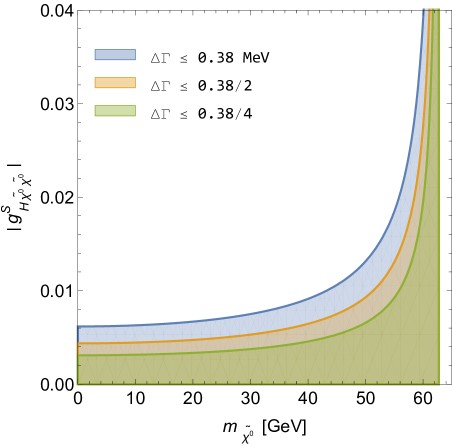
Figure 33: The allowed parameter space on the ($m_{\widetilde{\chi}_{1}^{0}}$, $|g^{S}_{H\widetilde{\chi}_{1}^{0}\widetilde{\chi}_{1}^{0}}|$) plane from $\Delta\Gamma_{\rm tot}\leq 0.38$ MeV at 95% CL. Also shown are future prospects assuming two and four times stronger constraints on $\Delta\Gamma_{\rm tot}$.

In the MSSM, there still exists a room for the lightest neutralino ${\widetilde{\chi}_{1}^{0}}$ to be light with its mass two times smaller than $M_{H}=125.5\,{\rm GeV}$ [292]. In this case, again, $\Delta\Gamma_{\rm tot}\leq 0.38$ MeV may provide 95% CL constraints on the mass $m_{\widetilde{\chi}_{1}^{0}}$ and the absolute value of the coupling $g^{S}_{H\widetilde{\chi}_{1}^{0}\widetilde{\chi}_{1}^{0}}$ assuming $H$ is purely CP even. We find $|g^{S}_{H\widetilde{\chi}_{1}^{0}\widetilde{\chi}_{1}^{0}}|\raisebox{-3.69899pt}{~{}\shortstack{$<$ \\ [-0.07cm] $\sim$}}~{}0.01$ for $m_{\widetilde{\chi}_{1}^{0}}\raisebox{-3.69899pt}{~{}\shortstack{$<$ \\ [-0.07cm] $\sim$}}~{}45$ GeV, see Fig. 33.

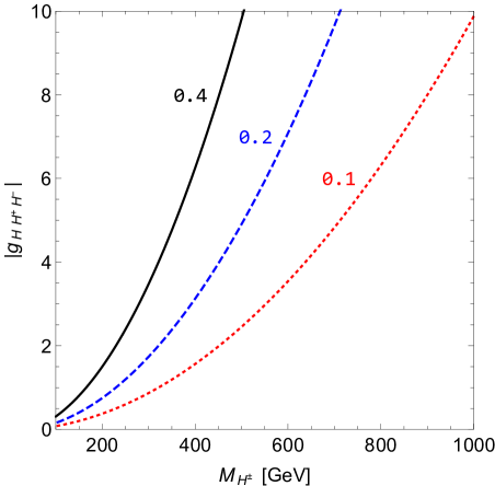
Figure 34: (Left) Contour lines for $|\Delta S^{\gamma}|=0.4\,,0.2\,,0.1$ from left to right on the ($m_{\widetilde{\chi}_{1}^{\pm}}$, $|g_{H\widetilde{\chi}_{1}^{+}\widetilde{\chi}_{1}^{-}}|$) plane assuming the lighter-chargino-loop contributions dominate $\Delta S^{\gamma}$. (Right) The same as in the left panel but on the ($M_{H^{\pm}}$, $|g_{HH^{+}H^{-}}|$) plane now assuming $\Delta S^{\gamma}$ is dominated by the contributions from charged-Higgs loops. For the reference value of $|\Delta S^{\gamma}|=0.4$, we are taking the $1\sigma$ error of the CPCN4 fit.

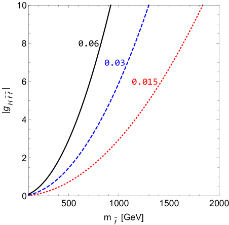
Figure 35: Contour lines for $|\Delta S^{g}|=0.06\,,0.03\,,0.015$ from left to right on the ($m_{\widetilde{t}_{1}}$, $|g_{H\widetilde{t}_{1}^{*}\widetilde{t}_{1}}|$) plane assuming $\Delta S^{g}$ is dominated by the contributions from the lighter-stop loops. For the reference value of $|\Delta S^{g}|=0.06$, we are taking the $1\sigma$ error of the CPCN4 fit.

From Table 11, we find $|\Delta S^{\gamma}|\raisebox{-3.69899pt}{~{}\shortstack{$<$ \\ [-0.07cm] $\sim$}}~{}0.4$ and $|\Delta S^{g}|\raisebox{-3.69899pt}{~{}\shortstack{$<$ \\ [-0.07cm] $\sim$}}~{}0.06$ by taking the errors in the CPCN4 fit. Exploiting these constraints, we derive constraints on the $H$ couplings to a pair of charged Higgs bosons, lighter charginos, and the lightest stops/sbottoms. For the SUSY contributions to $\Delta S^{\gamma}$ and $\Delta S^{g}$, we refer to Appendix B.

In the left panel of Fig. 34, we show the contour lines for $|\Delta S^{\gamma}|=0.4\,,0.2\,,0.1$ assuming it is dominated by the contributions from the lighter-chargino loops and considering only them. We find that the mass of the lighter chargino is constrained to be $m_{\widetilde{\chi}_{1}^{\pm}}\raisebox{-3.69899pt}{~{}\shortstack{$>$ \\ [-0.07cm] $\sim$}}~{}390$ GeV by the current LHC Higgs data when the relevant coupling is assumed to be 1. The lower-bound constraint on $m_{\widetilde{\chi}_{1}^{\pm}}$ linearly increases as the bound on $|\Delta S^{\gamma}|$ becomes stronger. In the right panel of Fig. 34, we show the same contour lines now assuming that $\Delta S^{\gamma}$ is dominated by the charged-Higgs loops. In the 2HDM and the MSSM, keeping the most significant three contributions when $M_{H_{2,3}}\raisebox{-3.69899pt}{~{}\shortstack{$>$ \\ [-0.07cm] $\sim$}}~{}v$, we find that the $g_{{}_{H_{1}H^{+}H^{-}}}$ coupling is given by

$$g_{{}_{H_{1}H^{+}H^{-}}} \sim 30\,\left(\frac{M_{H^{\pm}}}{\rm 1\,TeV}\right)^{2}+5\left[2\left(\frac{t_{\beta}}{30}\right)-\left(\frac{400\,{\rm GeV}}{M_{23}}\right)^{2}\left(\frac{t_{\beta}^{2}-1}{t_{\beta}^{2}}\right)\left(\frac{t_{\beta}}{30}\right)^{2}\right]\left(\frac{1+t_{\beta}^{2}}{t_{\beta}^{2}}\right)\left[\frac{\Re{\rm e}(m_{12}^{2}{\rm e}^{i\xi})}{(100\,{\rm GeV})^{2}}\right]\,$$ (243)

$$\hskip 74.54607pt-14\,\left(\frac{400\,{\rm GeV}}{M_{23}}\right)^{2}\,\left(\frac{1+t_{\beta}^{2}}{t_{\beta}^{2}}\right)\left(\frac{t_{\beta}}{30}\right)^{2}\,\Re{\rm e}{(\lambda_{7}{\rm e}^{i\xi})}\,,$$

under the assumption that $H_{1}$ is purely CP even state. Note that the second and the third terms contain contributions enhanced by the factors of $t_{\beta}$ and $t_{\beta}^{2}$ and, for the $t_{\beta}^{2}$-enhanced contributions, we are taking $M_{H_{2}}\sim M_{H_{3}}\equiv M_{23}$ and $c_{\beta-\alpha}=\sqrt{\epsilon}=\sqrt{\delta_{2}^{2}+\delta_{3}^{2}}=\sqrt{2\epsilon_{0}}\,M_{H_{1}}^{2}/M_{23}^{2}$ with $\epsilon_{0}=0.05$ as in the subsubsection 3.7.2, see Eq. (223). It is worthwhile to note that $\Delta S^{\gamma}_{1}(H^{\pm})\to 1/3$ when $M_{H^{\pm}}^{2}\,,M_{H_{2,3}}^{2}\gg M_{H_{1}}^{2}\,,v^{2}\,,\Re{\rm e}({m_{12}^{2}{\rm e}^{i\xi}})$, see Eq. (E) and the two equations following it. The constraint on $M_{H^{\pm}}$ becomes two times stronger when the bound on $|\Delta S^{\gamma}|$ becomes four times stronger.

In Fig. 35, we show the contour lines for $|\Delta S^{g}|=0.06\,,0.03\,,0.015$ assuming that it is dominated by the contributions from the lighter-stop loops. The current LHC Higgs data constrain the mass of the lighter stop as $m_{\widetilde{t}_{1}}\raisebox{-3.69899pt}{~{}\shortstack{$>$ \\ [-0.07cm] $\sim$}}~{}1$ TeV only when the relevant coupling is as large as 10 and, otherwise, it is weaker or much weaker than several direct bounds on the lighter-stop mass [6].

6 Conclusions

In this review, we have calculated and discussed in detail all the decay widths and branching fractions of Higgs bosons in the frameworks of the SM and its BSM extensions such as cxSM, 2HDMs with natural flavor conservation, and MSSM. We have allowed for CP-violating complex phases as generally as possible which induce CP-violating mixing among the neutral Higgs bosons. We have included the relevant higher order corrections, which are dominated by QCD corrections, as much as possible.

Firstly, the comprehensive analytical results presented in this review can be applied for not only presenting but also understanding all the details of calculating the decay widths of the neutral Higgs boson discovered at the LHC by allowing for nontrivial pseudoscalar as well as scalar couplings of the Higgs boson to fermions pairs. In the SM limit, it turned out that our numerical results solely based on the analytic expressions and supplemental materials provided in this review show good consistency with those presented by, for example, the LHC Higgs Cross Section Working Group implementing the state-of-the-art theoretical calculations [84]. We expect that the analytic expressions for LO decay widths and QCD corrections together with the SM ELW corrections presented in this review could be used for analyzing the decays of neutral Higgs bosons appearing in BSM models with the precision comparable to that achieved through the full-fledged theoretical calculations.

The second application of our analytical results was to the neutral 2HDM Higgs sector in the presence of nontrivial CP-violating phases of the complex quartic couplings. Specifically, we have taken the scenario where the lightest Higgs boson is purely CP even while the two heavier Higgs bosons are CP-mixed states exhibiting maximal CP violation when they are degenerate. To illustrate the typical decay patterns of the CP-violating heavy neutral Higgs bosons, we have taken the type-I 2HDM and we have contrasted them with those of purely CP-even or CP-odd neutral heavy Higgs bosons. Incidentally, we also have presented the decay pattern of a charged Higgs boson appearing in the framework of 2HDMs.

Thirdly, we have presented the constraints on the couplings of the Higgs boson weighing about 125 GeV obtained from implementing the global fits to all the Tevatron and LHC data available up to the summer in 2018. The global fits were based on several scenarios of the couplings and form factors for the main Higgs production and decay modes. Generally, the constraints turned out to be already tight on the tree-level couplings with the possibility that the loop-induced couplings could deviate sizably from the SM predictions.

Finally, we emphasize that, even with this comprehensive review, there remain lots of improvements for the QCD and electroweak corrections to be made so as to match the expected ever-increasing precision measurements from upgraded LHC and future high energy collider experiments. Furthermore, to draw a more unified picture for the genuine BSM physics, many BSM scenarios considered seriously at present and expected to be developed fully in a concrete form in the near future have to be included.

Appendices

This section consists of six appendices. Appendix A is for a summary of the SM parameters used for the numerical estimates of the Higgs decay widths and a description of the running of the strong coupling constant and quark masses. Appendix B is for the supersymmetric contributions to the loop-induced couplings of the Higgs boson to two gluons, two photons and $Z\gamma$. Appendix C is for the QCD corrections to the partial width of the Higgs-boson decay to two photons. We work out the relations among the parameters of the most general 2HDM in Appendix D and we apply them for deriving cubic Higgs-boson self-couplings in Appendix E. Finally, in Appendix F we briefly introduce a few well-developed numerical packages for calculating precise SM and full BSM-dependent ELW corrections.

Appendix A Standard Model Parameters

In this appendix, we summarize the SM parameters used for the estimation of decay widths of Higgs bosons. And we also show the running of the strong coupling constant and quark masses.

A.1 Input parameters

The SM parameters used for the estimation of decay widths of Higgs bosons are [6, 84]:

• Gauge coupling strengths

  $$\alpha_{s}(M_{Z}) = 0.118\pm 0.0015\,,$$

  $$\alpha(0) = 1/137.035999\,,$$

  $$\alpha(M_{W}) = 1/128\,.$$ (A.1)

• Electroweak parameters

  $$M_{W} = (80.385\pm 0.015)~{}\mathrm{GeV}\,,\ \ \ \ \ \ \Gamma_{W}=(2.085\pm 0.042)~{}\mathrm{GeV}\,;$$

  $$M_{Z} = (91.1876\pm 0.0021)~{}\mathrm{GeV}\,,\ \ \ \Gamma_{Z}=(2.4952\pm 0.0023)~{}\mathrm{GeV}\,;$$

  $$G_{F} = 1.1663787(6)\times 10^{-5}~{}\mathrm{GeV}^{-2}\,.$$ (A.2)

  The vev $v$ of the SM Higgs field is given by $v=\left(\sqrt{2}G_{F}\right)^{-1/2}\simeq 246.22$ GeV with $G_{F}=\sqrt{2}g^{2}/8M_{W}^{2}$ and $v=2M_{W}/g$. For the square of the sine of the weak mixing angle, we adopt the so-called on-shell scheme in which the tree-level relation $s_{W}^{2}=1-M^{2}_{W}/M^{2}_{Z}$ is promoted to define the renormalized $s_{W}^{2}$ to all orders in perturbation theory [293]: $s^{2}_{W}=0.22290$, $c_{W}^{2}=1-s^{2}_{W}=0.77710$, $g(M_{W})=e/s_{W}\simeq 0.66366$ and $g^{\prime}(M_{W})=e/c_{W}\simeq 0.35544$ with $e=e(M_{W})=2\sqrt{\pi\alpha(M_{W})}=0.31333$.

• Lepton masses

  $$M_{\mu}=(105.6583715\pm 0.00000035)~{}\mathrm{MeV}\,,\ \ \ M_{\tau}=(1776.82\pm 0.16)~{}\mathrm{MeV}\,.$$ (A.3)

• Quark masses

  $$M_{t} = (172.5\pm 1)~{}\mathrm{GeV}\,,$$

  $$\overline{m}_{b}(\overline{m}_{b}) = (4.18\pm 0.03)~{}\mathrm{GeV}\,,$$

  $$\overline{m}_{c}(3\,\mathrm{GeV}) = (0.986\pm 0.026)~{}\mathrm{GeV}\,.$$ (A.4)

  Note that the pole mass is used for $t$ quark while, for $b$ and $c$ quarks, $\overline{\rm MS}$ masses are used.

A.2 Running of the strong coupling constant and quark masses

We neglect the running of the SU(2)_L and U(1)_Y electroweak couplings and the leptons masses, measured experimentally with great precision. For the running of the strong coupling strength $\alpha_{s}(\mu)$ and the $\overline{\rm MS}$ quark masses $\overline{m}_{q}(\mu)$, we use the most recent version of RunDec [294, 295] in which five-loop corrections of the QCD beta function and four-loop decoupling effects are included. The results are shown in Fig. 36 and Table 12. We note that $\alpha_{s}(125.5\,{\rm GeV})=0.1126$ and $\overline{m}_{t}(M_{t})=161.5$ GeV. For the pole mass of $b$ quark, the three-loop conversion relation is taken to give $M_{b}=4.93$ GeV [6]. On the other hand, for the pole mass of $c$ quark, we take the relation between the on-shell charm-quark and bottom-quark masses, giving $M_{c}=M_{b}-3.41~{}{\rm GeV}=1.52$ GeV [6, 84, 296].

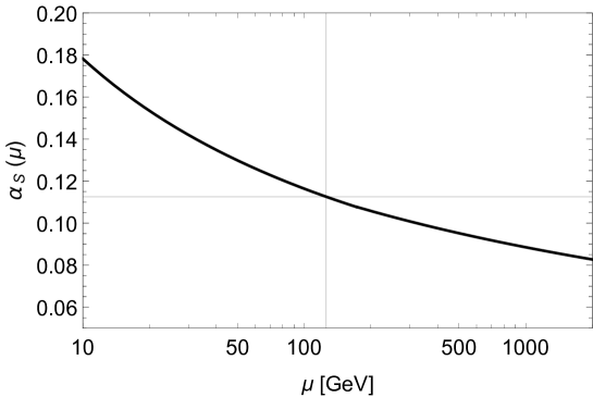
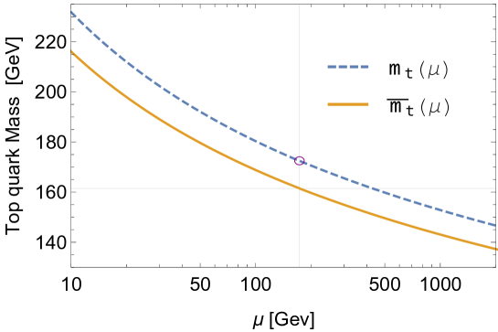
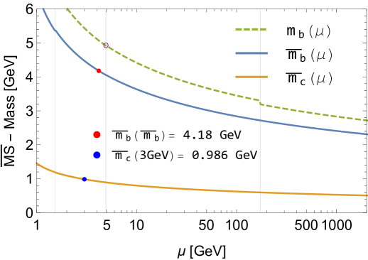
Figure 36: Running of the strong coupling constant $\alpha_{s}(\mu)$ (upper) and the $\overline{\rm MS}$ quark masses $\overline{m}_{t}(\mu)$ (middle) and $\overline{m}_{b,c}(\mu)$ (lower). In the upper frame, the vertical line locates the position of $M_{H}=125.5$ GeV. In the middle and lower frames, we also show $m_{t,b}(\mu)$ used in the calculations of $\Gamma(H\to\gamma\gamma)$ with the expressions given in Eq. (A.5). The vertical lines locate the positions of the pole masses of $M_{t}$ and $M_{b,c}$. And, in the lower frame, the input values for $b$ and $c$ quark masses are denoted by bullets, see Eq. (• ‣ A.1). The open circles in the middle and lower frames denote the positions $m_{t}(\mu=M_{t})=M_{t}$ and $m_{b}(\mu=M_{b})=M_{b}$, respectively, with $M_{t}=172.5$ GeV and $M_{b}=4.93$ GeV.

Table 12: Running of $\alpha_{s}(\mu)$, $\overline{m}_{c}(\mu)$, $\overline{m}_{b}(\mu)$, and $\overline{m}_{t}(\mu)$. $M_{q}^{+}$ and $M_{q-}$ are introduced for decoupling effects from matching the (effective) theory with $N_{F}-1$ with the (full) theory with $N_{F}$ at the scale $M_{q}$.

$\mu$ [GeV]	$\alpha_{s}(\mu)$	$\overline{m}_{c}(\mu)$ [GeV]	$\overline{m}_{b}(\mu)$ [GeV]	$\overline{m}_{t}(\mu)$ [GeV]
$1.52^{+}\,(M_{c}^{+})$	$3.48\times 10^{-1}$	$1.19\times 10^{0}\,~{}$	$5.40\times 10^{0}$	$3.21\times 10^{2}$
$3$	$2.54\times 10^{-1}$	$9.86\times 10^{-1}$	$4.47\times 10^{0}$	$2.66\times 10^{2}$
$4.18\,(\overline{m}_{b})$	$2.25\times 10^{-1}$	$9.21\times 10^{-1}$	$4.18\times 10^{0}$	$2.48\times 10^{2}$
$4.93_{-}\,(M_{b-})$	$2.13\times 10^{-1}$	$8.94\times 10^{-1}$	$4.06\times 10^{0}$	$2.41\times 10^{2}$
$4.93^{+}\,(M_{b}^{+})$	$2.14\times 10^{-1}$	$8.92\times 10^{-1}$	$4.06\times 10^{0}$	$2.41\times 10^{2}$
$10$	$1.78\times 10^{-1}$	$8.00\times 10^{-1}$	$3.64\times 10^{0}$	$2.16\times 10^{2}$
$20$	$1.53\times 10^{-1}$	$7.32\times 10^{-1}$	$3.33\times 10^{0}$	$1.98\times 10^{2}$
$30$	$1.42\times 10^{-1}$	$7.00\times 10^{-1}$	$3.18\times 10^{0}$	$1.89\times 10^{2}$
$40$	$1.35\times 10^{-1}$	$6.79\times 10^{-1}$	$3.09\times 10^{0}$	$1.84\times 10^{2}$
$50$	$1.30\times 10^{-1}$	$6.65\times 10^{-1}$	$3.02\times 10^{0}$	$1.80\times 10^{2}$
$60$	$1.26\times 10^{-1}$	$6.54\times 10^{-1}$	$2.97\times 10^{0}$	$1.77\times 10^{2}$
$70$	$1.23\times 10^{-1}$	$6.44\times 10^{-1}$	$2.93\times 10^{0}$	$1.74\times 10^{2}$
$80$	$1.20\times 10^{-1}$	$6.37\times 10^{-1}$	$2.90\times 10^{0}$	$1.72\times 10^{2}$
$90$	$1.18\times 10^{-1}$	$6.30\times 10^{-1}$	$2.87\times 10^{0}$	$1.70\times 10^{2}$
$100$	$1.16\times 10^{-1}$	$6.25\times 10^{-1}$	$2.84\times 10^{0}$	$1.69\times 10^{2}$
$110$	$1.15\times 10^{-1}$	$6.20\times 10^{-1}$	$2.82\times 10^{0}$	$1.67\times 10^{2}$
$120$	$1.13\times 10^{-1}$	$6.15\times 10^{-1}$	$2.80\times 10^{0}$	$1.66\times 10^{2}$
$125.5$	$1.13\times 10^{-1}$	$6.13\times 10^{-1}$	$2.79\times 10^{0}$	$1.66\times 10^{2}$
$130$	$1.12\times 10^{-1}$	$6.11\times 10^{-1}$	$2.78\times 10^{0}$	$1.65\times 10^{2}$
$140$	$1.11\times 10^{-1}$	$6.08\times 10^{-1}$	$2.76\times 10^{0}$	$1.64\times 10^{2}$
$150$	$1.10\times 10^{-1}$	$6.04\times 10^{-1}$	$2.75\times 10^{0}$	$1.63\times 10^{2}$
$160$	$1.09\times 10^{-1}$	$6.01\times 10^{-1}$	$2.73\times 10^{0}$	$1.62\times 10^{2}$
$170$	$1.08\times 10^{-1}$	$5.98\times 10^{-1}$	$2.72\times 10^{0}$	$1.62\times 10^{2}$
$172.5_{-}\,(M_{t-})$	$1.08\times 10^{-1}$	$5.98\times 10^{-1}$	$2.72\times 10^{0}$	$1.62\times 10^{2}$
$172.5^{+}\,(M_{t}^{+})$	$1.08\times 10^{-1}$	$5.98\times 10^{-1}$	$2.72\times 10^{0}$	$1.61\times 10^{2}$
$180$	$1.07\times 10^{-1}$	$5.96\times 10^{-1}$	$2.71\times 10^{0}$	$1.61\times 10^{2}$
$190$	$1.06\times 10^{-1}$	$5.93\times 10^{-1}$	$2.70\times 10^{0}$	$1.60\times 10^{2}$
$200$	$1.06\times 10^{-1}$	$5.91\times 10^{-1}$	$2.69\times 10^{0}$	$1.60\times 10^{2}$
$300$	$1.01\times 10^{-1}$	$5.74\times 10^{-1}$	$2.61\times 10^{0}$	$1.55\times 10^{2}$
$400$	$9.76\times 10^{-2}$	$5.62\times 10^{-1}$	$2.56\times 10^{0}$	$1.52\times 10^{2}$
$500$	$9.52\times 10^{-2}$	$5.54\times 10^{-1}$	$2.52\times 10^{0}$	$1.50\times 10^{2}$
$1000$	$8.85\times 10^{-2}$	$5.29\times 10^{-1}$	$2.41\times 10^{0}$	$1.43\times 10^{2}$

Specifically for the loop-induced decay $H\to\gamma\gamma$, we use the running masses $m_{t,b}(\mu)$ of which the expressions are given at the four-loop level by [148, 297]

$$m_{q}(\mu)=M_{q}\,\Bigg{[}\frac{\alpha_{s}(\mu)}{\alpha_{s}(M_{q})}\Bigg{]}^{12/(33-2\,N_{F})}\,\frac{1+c_{1}^{q}\left[\frac{\alpha_{s}(\mu)}{\pi}\right]+c_{2}^{q}\left[\frac{\alpha_{s}(\mu)}{\pi}\right]^{2}+c_{3}^{q}\left[\frac{\alpha_{s}(\mu)}{\pi}\right]^{3}}{1+c_{1}^{q}\left[\frac{\alpha_{s}(M_{q})}{\pi}\right]+c_{2}^{q}\left[\frac{\alpha_{s}(M_{q})}{\pi}\right]^{2}+c_{3}^{q}\left[\frac{\alpha_{s}(M_{q})}{\pi}\right]^{3}}\,,$$ (A.5)

where the numerical values of the six dimensionless coefficients are

$$c_{1}^{b} = 1.17549\,,\ \ \ c_{2}^{b}=1.50071\,,\ \ \ c_{3}^{b}=0.172478\,;$$

$$c_{1}^{t} = 1.39796\,,\ \ \ c_{2}^{t}=1.79348\,,\ \ \ c_{3}^{t}=-0.683433\,.$$ (A.6)

Note that $m_{q}(M_{q})=M_{q}$ as denoted by open circles in the middle and lower frames in Fig. 36.

Appendix B Supersymmetric Contributions to the $Hgg$, $H\gamma\gamma$, and $HZ\gamma$ Form Factors

In this appendix, we present the contributions to the loop-induced $Hgg$, $H\gamma\gamma$, and $HZ\gamma$ form factors from the triangle diagrams in which charginos, charged and/or colored sfermions, and/or charged Higgs bosons are running.

In the minimal supersymmetric extension of the SM (MSSM), the form factors of $\Delta S^{g,\gamma}$ and $\Delta P^{g,\gamma}$ denoting new MSSM contributions to the $Hgg,H\gamma\gamma$ vertices are given by:

$$\Delta S^{g}_{i} = -\sum_{\widetilde{f}_{j}=\widetilde{t}_{1},\widetilde{t}_{2},\widetilde{b}_{1},\widetilde{b}_{2}}g_{H_{i}\widetilde{f}^{*}_{j}\widetilde{f}_{j}}\frac{v^{2}}{4m_{\widetilde{f}_{j}}^{2}}F_{0}(\tau_{i\widetilde{f}_{j}})\,,$$

$$\Delta P^{g}_{i} = 0\,;$$ (B.1)

$$\Delta S^{\gamma}_{i} = \sqrt{2}\,g\sum_{f=\widetilde{\chi}^{\pm}_{1},\widetilde{\chi}^{\pm}_{2}}g^{S}_{H_{i}\bar{f}f}\,\frac{v}{m_{f}}F_{sf}(\tau_{if})-\sum_{\widetilde{f}_{j}=\widetilde{t}_{1},\widetilde{t}_{2},\widetilde{b}_{1},\widetilde{b}_{2},\widetilde{\tau}_{1},\widetilde{\tau}_{2}}N_{C}^{f}\,Q_{f}^{2}g_{H_{i}\widetilde{f}^{*}_{j}\widetilde{f}_{j}}\frac{v^{2}}{2m_{\widetilde{f}_{j}}^{2}}F_{0}(\tau_{i\widetilde{f}_{j}})$$

$$+g_{{}_{H_{i}H^{+}H^{-}}}\frac{v^{2}}{2M_{H^{\pm}}^{2}}F_{0}(\tau_{iH^{\pm}})\,,$$

$$\Delta P^{\gamma}_{i} = \sqrt{2}\,g\sum_{f=\widetilde{\chi}^{\pm}_{1},\widetilde{\chi}^{\pm}_{2}}g^{P}_{H_{i}\bar{f}f}\,\frac{v}{m_{f}}F_{pf}(\tau_{if})\,,$$ (B.2)

where $\tau_{ix}=M_{H_{i}}^{2}/4m_{x}^{2}$ with $i=1,2,3$ denoting three neutral Higgs bosons and $N_{C}^{f}=3$ for (s)quarks and $N_{C}^{f}=1$ for status, respectively. The form factor $F_{0}(\tau)$ is given by

$$F_{0}(\tau)=\tau^{-1}\,[-1+\tau^{-1}f(\tau)]\,,$$ (B.3)

which takes the value of $1/3$ when $\tau=0$, see Fig. 8.

On the other hand, the form factors of $\Delta S^{Z\gamma}$ and $\Delta P^{Z\gamma}$ denoting new MSSM contributions to the $HZ\gamma$ vertices may take forms of [227]

$$\Delta S_{i}^{Z\gamma}\, = -\sqrt{2}\,\frac{g}{c_{W}s_{W}}\sum_{j,k}v\,m_{\widetilde{\chi}_{j}^{\pm}}f\left(m_{\widetilde{\chi}_{j}^{\pm}},m_{\widetilde{\chi}_{k}^{\pm}},m_{\widetilde{\chi}_{k}^{\pm}}\right)v_{Z\widetilde{\chi}_{j}^{+}\widetilde{\chi}_{k}^{-}}g^{S}_{H_{i}\widetilde{\chi}_{k}^{+}\widetilde{\chi}_{j}^{-}}$$

$$-4\sum_{f=t,b,\tau}\frac{N_{C}^{f}Q_{f}}{c_{W}s_{W}}\left[\sum_{j,k}g_{H_{i}\widetilde{f}_{j}^{*}\widetilde{f}_{k}}g_{Z\widetilde{f}_{k}^{*}\widetilde{f}_{j}}\,v^{2}\,C_{2}(m_{\widetilde{f}_{j}},m_{\widetilde{f}_{k}},m_{\widetilde{f}_{k}})\right]$$

$$+2\,\frac{g_{H_{i}H^{+}H^{-}}}{c_{W}s_{W}}\,\frac{v^{2}}{M_{H^{\pm}}^{2}}\,I_{1}\left(\tau_{iH^{\pm}},\lambda_{H^{\pm}}\right)\,,$$

$$\Delta P_{i}^{Z\gamma}\, = -\sqrt{2}\,\frac{i\,g}{c_{W}s_{W}}\sum_{j,k}v\,m_{\widetilde{\chi}_{j}^{\pm}}g\left(m_{\widetilde{\chi}_{j}^{\pm}},m_{\widetilde{\chi}_{k}^{\pm}},m_{\widetilde{\chi}_{k}^{\pm}}\right)v_{Z\widetilde{\chi}_{j}^{+}\widetilde{\chi}_{k}^{-}}g^{P}_{H_{i}\widetilde{\chi}_{k}^{+}\widetilde{\chi}_{j}^{-}}\,,$$ (B.4)

where $\tau_{iH^{\pm}}=M_{H_{i}}^{2}/4M_{H^{\pm}}^{2}$ with $i=1,2,3$, $\lambda_{H^{\pm}}=M_{Z}^{2}/4M_{H^{\pm}}^{2}$, and $N_{C}^{f}=3$ for squarks and $N_{C}^{f}=1$ for staus, respectively. For the explicit form of the three loop functions of $f(m_{1},m_{2},m_{2})$, $g(m_{1},m_{2},m_{2})$, and $C_{2}(m_{1},m_{2},m_{2})$, we refer to [227]. Note that they implicitly depend on $M_{H_{i}}^{2}$ and $M_{Z}^{2}$. For the Higgs couplings to SUSY particles, see subsubsection 2.4.3 and the relevant $Z$-boson interactions are given by the following Lagrangian terms:

• $Z$-sfermion-sfermion

  $${\cal L}_{Z\widetilde{f}\widetilde{f}}\ =\ -ig_{Z}\,g_{Z\widetilde{f}_{j}^{*}\widetilde{f}_{i}}\ \left(\widetilde{f}_{j}^{*}\stackrel{{\scriptstyle\leftrightarrow}}{{\partial_{\mu}}}\widetilde{f}_{i}\right)\ Z^{\mu}\,,$$ (B.5)

  where $g_{Z}=e/(s_{W}c_{W})$ and

  $$g_{Z\widetilde{f}_{j}^{*}\widetilde{f}_{i}}\ =\ I_{3}^{f}U_{Lj}^{\widetilde{f}*}U_{Li}^{\widetilde{f}}-Q_{f}s_{W}^{2}\delta_{ij}\,,$$ (B.6)

  with $I_{3}^{\,u,\nu}=+1/2$ and $I_{3}^{\,d,e}=-1/2$.

• $Z$-chargino-chargino

  $${\cal L}_{Z\widetilde{\chi}^{+}\widetilde{\chi}^{-}}=-\,g_{Z}\,\overline{\widetilde{\chi}^{-}_{i}}\,\gamma^{\mu}\,\left(v_{Z\chi^{+}_{i}\widetilde{\chi}^{-}_{j}}-a_{Z\chi^{+}_{i}\widetilde{\chi}^{-}_{j}}\gamma_{5}\right)\,\widetilde{\chi}^{-}_{j}\,Z_{\mu}\,,$$ (B.7)

  where the vector and axial–vector couplings are given by

  $$v_{Z\chi^{+}_{i}\widetilde{\chi}^{-}_{j}} = \frac{1}{4}\left[\left(C_{L}\right)_{i2}\left(C_{L}\right)_{j2}^{*}+\left(C_{R}\right)_{i2}\left(C_{R}\right)_{j2}^{*}\right]\ -\ c_{W}^{2}\,\delta_{ij}\,,$$

  $$a_{Z\chi^{+}_{i}\widetilde{\chi}^{-}_{j}} = \frac{1}{4}\left[\left(C_{L}\right)_{i2}\left(C_{L}\right)_{j2}^{*}-\left(C_{R}\right)_{i2}\left(C_{R}\right)_{j2}^{*}\right]\,.$$ (B.8)

  For completeness, we recall that the $Z$-boson couplings to the quarks and leptons are given by

  $${\cal L}_{Z\bar{f}f}=-\,g_{Z}\,\bar{f}\,\gamma^{\mu}\,\left(v_{Z\bar{f}f}-a_{Z\bar{f}f}\gamma_{5}\right)\,f\,Z_{\mu}\,,$$ (B.9)

  with $v_{Z\bar{f}f}=I_{3}^{f}/2-Q_{f}s_{W}^{2}$ and $a_{Z\bar{f}f}=I_{3}^{f}/2$ in terms of the third component of weak isospin $I^{f}_{3}$ and the electric charge $Q_{f}$ of each fermion $f$.

Appendix C QCD Corrections to $\Gamma(H\to\gamma\gamma)$: $C_{sf}(\tau)$ and $C_{pf}(\tau)$

The scaling factors $C_{sf}(\tau)$ and $C_{pf}(\tau)$ for the QCD corrections to the decay width of a Higgs boson $H$ into two photons might be given by [183]

$$C_{sf}(\tau;\rho)=C_{1}^{H}(\tau)+C_{2}^{H}(\tau)\left[\log\tau+\log\frac{4}{\rho^{2}}\right]\,;\ \ \ C_{pf}(\tau;\rho)=C_{1}^{A}(\tau)+C_{2}^{A}(\tau)\left[\log\tau+\log\frac{4}{\rho^{2}}\right]\,,$$ (C.1)

where $\tau=M_{H}^{2}/4m_{q}^{2}(\mu_{q})$ with the renormalization scale $\mu_{q}=M_{H}/\rho$. As demonstrated in Section 3.5, we take $\rho=2$. We note again the running mass $m_{q}$ is normalized as $m_{q}(M_{q})=M_{q}$.

The $C_{1}^{H}(\tau)$ function is given via the following relation [212, 213]

$$F_{sf}(\tau)\,C_{1}^{H}(\tau) = -\frac{2\,\theta\left(1+\theta+\theta^{2}+\theta^{3}\right)}{3\,{\left(1-\theta\right)}^{5}}\biggl{[}108\,{\rm Li}_{4}(\theta)+144\,{\rm Li}_{4}(-\theta)-64\,{\rm Li}_{3}(\theta)\ln\theta$$ (C.2)

$$\hskip 28.45274pt-64\,{\rm Li}_{3}(-\theta)\ln\theta+14\,{\rm Li}_{2}(\theta)\ln^{2}\theta+8\,{\rm Li}_{2}(-\theta)\ln^{2}\theta+\frac{1}{12}\ln^{4}\theta$$

$$\hskip 28.45274pt+4\,\zeta_{2}\ln^{2}\theta+16\,\zeta_{3}\ln\theta+18\,\zeta_{4}\biggr{]}$$

$$+\frac{2\,\theta{\left(1+\theta\right)}^{2}}{3\,{\left(1-\theta\right)}^{4}}\biggl{[}-32\,{\rm Li}_{3}(-\theta)+16\,{\rm Li}_{2}(-\theta)\ln\theta-4\,\zeta_{2}\ln\theta\biggr{]}$$

$$-\frac{8\,\theta\left(7-2\,\theta+7\,\theta^{2}\right)}{3\,{\left(1-\theta\right)}^{4}}\,{\rm Li}_{3}(\theta)+\frac{16\,\theta\left(3-2\,\theta+3\,\theta^{2}\right)}{3\,{\left(1-\theta\right)}^{4}}\,{\rm Li}_{2}(\theta)\ln\theta$$

$$+\frac{4\,\theta\left(5-6\,\theta+5\,\theta^{2}\right)}{3\,{\left(1-\theta\right)}^{4}}\ln(1-\theta)\ln^{2}\theta+\frac{2\theta\left(3+25\,\theta-7\,\theta^{2}+3\,\theta^{3}\right)}{9\,{\left(1-\theta\right)}^{5}}\ln^{3}\theta$$

$$+\frac{8\,\theta\left(1-14\,\theta+\theta^{2}\right)}{3\,{\left(1-\theta\right)}^{4}}\zeta_{3}+\frac{8\,\theta^{2}}{{\left(1-\theta\right)}^{4}}\ln^{2}\theta-\frac{8\,\theta\left(1+\theta\right)}{{\left(1-\theta\right)}^{3}}\ln\theta-\frac{40\,\theta}{3\,{\left(1-\theta\right)}^{2}}\,,$$

where $\theta$ is a $\tau$-dependent function defined by

$$\theta\equiv\theta(\tau)=\frac{\sqrt{1-\tau^{-1}}-1}{\sqrt{1-\tau^{-1}}+1}\,.$$ (C.3)

The three values, $\zeta_{2},\zeta_{3}$ and $\zeta_{4}$, of the Riemann’s zeta function are given by

$$\zeta_{2}=\frac{\pi^{2}}{6}\,,\quad\zeta_{3}=1.20205690\,,\quad\zeta_{4}=\frac{\pi^{4}}{90}\,,$$ (C.4)

and the polylogarithm function is defined by a power series in a complex variable $z$ as follows

$$\,{\rm Li}_{n}(z)=\sum_{k=1}^{\infty}\frac{z^{k}}{k^{n}}~{},~{}~{}n=1,2,3,\cdots\,.$$ (C.5)

For analytic continuation to the complex $\tau$ plane, the replacement $\tau\to\tau+0\,i$ is understood. The $C_{2}^{H}(\tau)$ function is given via [213]

$$F_{sf}(\tau)\,C_{2}^{H}(\tau)=2\,\tau^{-2}\left[\tau+\left(\tau-2\right)f(\tau)-(\tau-1)\tau\,\frac{{\rm d}f(\tau)}{{\rm d}\tau}\right]\,,$$ (C.6)

with the function $f(\tau)$ defined in Eq. (175).

On the other hand, the $C_{1}^{A}(\tau)$ and $C_{2}^{A}(\tau)$ functions are given via the following relations [213]

$$F_{pf}(\tau)\,C_{1}^{A}(\tau) = -\frac{\theta\left(1+\theta^{2}\right)}{{\left(1-\theta\right)}^{3}\left(1+\theta\right)}\Bigg{\{}72\,{\rm Li}_{4}(\theta)+96\,{\rm Li}_{4}(-\theta)-\frac{128}{3}\Big{[}\,{\rm Li}_{3}(\theta)+\,{\rm Li}_{3}(-\theta)\Big{]}\ln\theta$$ (C.7)

$$\hskip 93.89418pt+\frac{28}{3}\,{\rm Li}_{2}(\theta)\ln^{2}\theta+\frac{16}{3}\,{\rm Li}_{2}(-\theta)\ln^{2}\theta+\frac{1}{18}\ln^{4}\theta$$

$$\hskip 93.89418pt+\frac{8}{3}\zeta_{2}\ln^{2}\theta+\frac{32}{3}\zeta_{3}\ln\theta+12\zeta_{4}\Bigg{\}}$$

$$+\frac{\theta}{{\left(1-\theta\right)}^{2}}\biggl{[}-\frac{56}{3}\,{\rm Li}_{3}(\theta)-\frac{64}{3}\,{\rm Li}_{3}(-\theta)+16\,{\rm Li}_{2}(\theta)\ln\theta$$

$$\hskip 56.9055pt+\frac{32}{3}\,{\rm Li}_{2}(-\theta)\ln\theta+\frac{20}{3}\ln(1-\theta)\ln^{2}\theta-\frac{8}{3}\zeta_{2}\ln\theta+\frac{8}{3}\zeta_{3}\biggr{]}$$

$$+\frac{2\,\theta\left(1+\theta\right)}{{3\left(1-\theta\right)}^{3}}\,\ln^{3}\theta\,;$$

$$F_{pf}(\tau)\,C_{2}^{A}(\tau) = 2\,\tau^{-1}\left[f(\tau)-\tau\,\frac{{\rm d}f(\tau)}{{\rm d}\tau}\right]\,,$$ (C.8)

respectively.

Appendix D Input parameters for the most general 2HDM potential

In this appendix, we work out the relations among the parameters needed to fully specify the most general 2HDM potential, the masses of neutral and charged Higgs bosons, and the mixing matrix $O$.

In subsection 2.3, we demonstrate that one needs all the elements of the following set of parameters

$${\cal I}=\left\{v\,,t_{\beta}\,,|m_{12}|\,;\lambda_{1}\,,\lambda_{2}\,,\lambda_{3}\,,\lambda_{4}\,,|\lambda_{5}|\,,|\lambda_{6}|\,,|\lambda_{7}|\,,\phi_{5}+2\xi\,,\phi_{6}+\xi\,,\phi_{7}+\xi\,;{\rm sign}[\cos(\phi_{12}+\xi)]\right\}\,,$$ (D.1)

to fully specify the most general 2HDM scalar potential, see Eq. (2.3.1). The set ${\cal I}$ contains 13 parameters plus 1 sign with $\sin(\phi_{12}+\xi)$ being determined by the third CP-odd tadpole condition in Eq. (2.3.1). Alternatively to the set ${\cal I}$, one may use the following equivalent set

$${\cal I}^{\prime} = \{v\,,t_{\beta}\,,\Re{\rm e}(m_{12}^{2}{\rm e}^{i\xi})\,;$$

$$\hskip 5.69054pt\lambda_{1}\,,\lambda_{2}\,,\lambda_{3}\,,\lambda_{4}\,,\Re{\rm e}(\lambda_{5}{\rm e}^{2i\xi})\,,\Re{\rm e}(\lambda_{6}{\rm e}^{i\xi})\,,\Re{\rm e}(\lambda_{7}{\rm e}^{i\xi})\,,\Im{\rm m}(\lambda_{5}{\rm e}^{2i\xi})\,,\Im{\rm m}(\lambda_{6}{\rm e}^{i\xi})\,,\Im{\rm m}(\lambda_{7}{\rm e}^{i\xi})\}\,.$$

The above set ${\cal I}^{\prime}$ contains 10 parameters for the real and complex quartic couplings $\lambda_{1-7}$ and any 7 of them, in principle, can be traded with the 4 masses of charged and neutral Higgs bosons and the 3 independent angles of the $3\times 3$ orthogonal mixing matrix $O$ by judiciously exploiting Eq. (44) and the matrix relation $O^{T}{\cal M}_{0}^{2}O={\rm diag}(M_{H_{1}}^{2},M_{H_{2}}^{2},M_{H_{3}}^{2})$. By choosing $\Im{\rm m}(\lambda_{5}{\rm e}^{2i\xi})$, $\Re{\rm e}(\lambda_{6}{\rm e}^{i\xi})$, and $\Re{\rm e}(\lambda_{7}{\rm e}^{i\xi})$ as independent input parameters, one may use the following set of more physical parameters:

$${\cal P}=\{v\,,t_{\beta}\,,\Re{\rm e}(m_{12}^{2}{\rm e}^{i\xi})\,;M_{H_{1}}\,,M_{H_{2}}\,,M_{H_{3}}\,,M_{H^{\pm}}\,,\{O\}\,;\Im{\rm m}(\lambda_{5}{\rm e}^{2i\xi})\,,\Re{\rm e}(\lambda_{6}{\rm e}^{i\xi})\,,\Re{\rm e}(\lambda_{7}{\rm e}^{i\xi})\}\,.$$ (D.3)

Explicitly, we find that the 7 quartic couplings of $\lambda_{1}$, $\lambda_{2}$, $\lambda_{3}$, $\lambda_{4}$, $\Re{\rm e}(\lambda_{5}{\rm e}^{2i\xi})$, $\Im{\rm m}(\lambda_{6}{\rm e}^{i\xi})$, and $\Im{\rm m}(\lambda_{7}{\rm e}^{i\xi})$ in the set ${\cal I}^{\prime}$ can be expressed in terms of $M_{H_{1,2,3}}$, $M_{H^{\pm}}$, and the elements of the mixing matrix $O$ in the set ${\cal P}$ as follows:

$$\lambda_{1}=\frac{s_{\beta}}{2v^{2}c_{\beta}^{3}}\,\Re{\rm e}(m_{12}^{2}{\rm e}^{i\xi})+\frac{O_{\phi_{1}1}^{2}}{2v^{2}c_{\beta}^{2}}\,M_{H_{1}}^{2}+\frac{O_{\phi_{1}2}^{2}}{2v^{2}c_{\beta}^{2}}\,M_{H_{2}}^{2}+\frac{O_{\phi_{1}3}^{2}}{2v^{2}c_{\beta}^{2}}\,M_{H_{3}}^{2}-\frac{3t_{\beta}}{4}\Re{\rm e}{(\lambda_{6}{\rm e}^{i\xi})}+\frac{t_{\beta}^{3}}{4}\Re{\rm e}{(\lambda_{7}{\rm e}^{i\xi})}\,,$$

$$\lambda_{2}=\frac{c_{\beta}}{2v^{2}s_{\beta}^{3}}\,\Re{\rm e}(m_{12}^{2}{\rm e}^{i\xi})+\frac{O_{\phi_{2}1}^{2}}{2v^{2}s_{\beta}^{2}}\,M_{H_{1}}^{2}+\frac{O_{\phi_{2}2}^{2}}{2v^{2}s_{\beta}^{2}}\,M_{H_{2}}^{2}+\frac{O_{\phi_{2}3}^{2}}{2v^{2}s_{\beta}^{2}}\,M_{H_{3}}^{2}+\frac{1}{4t_{\beta}^{3}}\Re{\rm e}{(\lambda_{6}{\rm e}^{i\xi})}-\frac{3}{4t_{\beta}}\Re{\rm e}{(\lambda_{7}{\rm e}^{i\xi})}\,,$$

$$\lambda_{3}=\frac{1}{v^{2}s_{\beta}c_{\beta}}\Re{\rm e}(m_{12}^{2}{\rm e}^{i\xi})+\frac{2}{v^{2}}M_{H^{\pm}}^{2}+\frac{O_{\phi_{1}1}O_{\phi_{2}1}}{v^{2}s_{\beta}c_{\beta}}\,M_{H_{1}}^{2}+\frac{O_{\phi_{1}2}O_{\phi_{2}2}}{v^{2}s_{\beta}c_{\beta}}\,M_{H_{2}}^{2}+\frac{O_{\phi_{1}3}O_{\phi_{2}3}}{v^{2}s_{\beta}c_{\beta}}\,M_{H_{3}}^{2}$$

$$\hskip 28.45274pt-\frac{1}{2t_{\beta}}\Re{\rm e}{(\lambda_{6}{\rm e}^{i\xi})}-\frac{t_{\beta}}{2}\Re{\rm e}{(\lambda_{7}{\rm e}^{i\xi})}\,,$$

$$\lambda_{4}=-\frac{1}{v^{2}s_{\beta}c_{\beta}}\,\Re{\rm e}(m_{12}^{2}{\rm e}^{i\xi})-\frac{2}{v^{2}}M_{H^{\pm}}^{2}+\frac{O_{a1}^{2}}{v^{2}}\,M_{H_{1}}^{2}+\frac{O_{a2}^{2}}{v^{2}}\,M_{H_{2}}^{2}+\frac{O_{a3}^{2}}{v^{2}}\,M_{H_{3}}^{2}-\frac{1}{2t_{\beta}}\Re{\rm e}{(\lambda_{6}{\rm e}^{i\xi})}-\frac{t_{\beta}}{2}\Re{\rm e}{(\lambda_{7}{\rm e}^{i\xi})}\,,$$

$$\Re{\rm e}{(\lambda_{5}{\rm e}^{2i\xi})}=-\frac{1}{v^{2}s_{2\beta}}\,\Re{\rm e}(m_{12}^{2}{\rm e}^{i\xi})-\frac{O_{a1}^{2}}{2v^{2}}\,M_{H_{1}}^{2}-\frac{O_{a2}^{2}}{2v^{2}}\,M_{H_{2}}^{2}-\frac{O_{a3}^{2}}{2v^{2}}\,M_{H_{3}}^{2}-\frac{1}{4t_{\beta}}\Re{\rm e}{(\lambda_{6}{\rm e}^{i\xi})}-\frac{t_{\beta}}{4}\Re{\rm e}{(\lambda_{7}{\rm e}^{i\xi})}\,,$$

$$\Im{\rm m}{(\lambda_{6}{\rm e}^{i\xi})}=-\frac{O_{\phi_{1}1}O_{a1}}{v^{2}c_{\beta}}\,M_{H_{1}}^{2}-\frac{O_{\phi_{1}2}O_{a2}}{v^{2}c_{\beta}}\,M_{H_{2}}^{2}-\frac{O_{\phi_{1}3}O_{a3}}{v^{2}c_{\beta}}\,M_{H_{3}}^{2}-t_{\beta}\Im{\rm m}{(\lambda_{5}{\rm e}^{2i\xi})}\,,$$

$$\Im{\rm m}{(\lambda_{7}{\rm e}^{i\xi})}=-\frac{O_{\phi_{2}1}O_{a1}}{v^{2}s_{\beta}}\,M_{H_{1}}^{2}-\frac{O_{\phi_{2}2}O_{a2}}{v^{2}s_{\beta}}\,M_{H_{2}}^{2}-\frac{O_{\phi_{2}3}O_{a3}}{v^{2}s_{\beta}}\,M_{H_{3}}^{2}-\frac{1}{t_{\beta}}\Im{\rm m}{(\lambda_{5}{\rm e}^{2i\xi})}\,.$$ (D.4)

We find that our results are consistent with those presented in Refs. [298, 299]. We note that $\lambda_{2}$ can be obtained from $\lambda_{1}$ or vice versa by exchanging $c_{\beta}\leftrightarrow s_{\beta}$, $\phi_{1}\leftrightarrow\phi_{2}$, and $\lambda_{6}\leftrightarrow\lambda_{7}$. The same observation could be applied for $\Im{\rm m}{(\lambda_{6}{\rm e}^{i\xi})}$ and $\Im{\rm m}{(\lambda_{7}{\rm e}^{i\xi})}$ which are vanishing when each Higgs boson is purely CP-even or CP-odd state and $\Im{\rm m}{(\lambda_{5}{\rm e}^{2i\xi})}=0$. About $\lambda_{3}$ and $\lambda_{4}$, we note that $\lambda_{3}+\lambda_{4}$ is independent of $\Re{\rm e}(m_{12}^{2}{\rm e}^{i\xi})$ and $M_{H^{\pm}}^{2}$, the neutral Higgs mass contributions to $\lambda_{3}$ ($\lambda_{4}$) are involved with only the CP-even (CP-odd) components of each Higgs boson, and the contributions from $\Re{\rm e}{(\lambda_{6}{\rm e}^{i\xi})}$ and $\Re{\rm e}{(\lambda_{7}{\rm e}^{i\xi})}$ are in common. In passing, we check that Eq. (49) for the difference between $\lambda_{4}/2$ and $\Re{\rm e}{(\lambda_{5}{\rm e}^{2i\xi})}$ is satisfied by noting the relation $O_{a1}^{2}M_{H_{1}}^{2}+O_{a2}^{2}M_{H_{2}}^{2}+O_{a3}^{2}M_{H_{3}}^{2}=M_{A}^{2}$.

Appendix E Cubic Higgs-boson self-couplings in 2HDMs

In this appendix, we apply the relations among the 2HDM input parameters obtained in Appendix D to derive cubic Higgs-boson self-couplings when the lightest Higgs boson is purely CP even as assumed in subsubsection 3.7.2 by taking the following $O$ matrix:

$$O\ =\ \left(\begin{array}[]{ccc}-s_{\alpha}&c_{\alpha}c_{\omega}&c_{\alpha}s_{\omega}\\ ~{}~{}c_{\alpha}&s_{\alpha}c_{\omega}&s_{\alpha}s_{\omega}\\ ~{}0&-s_{\omega}&c_{\omega}\\ \end{array}\right)\,.$$ (E.1)

In this case, using Eq. (63), Eq. (2.3.4) for the cubic self–couplings of the Higgs weak eigenstates, and Eq. (D) for the conversion relations, we find the couplings of the heavy neural Higgs bosons $H_{2,3}$ to a pair of the lightest Higgs bosons are given by

$$g_{{}_{H_{2}\,H_{1}\,H_{1}\,}} = -\frac{c_{\omega}}{s_{2\beta}^{2}}\bigg{[}4s_{2\beta}c_{\beta-\alpha}+6c_{2\beta}s_{\beta-\alpha}c_{\beta-\alpha}^{2}-6s_{2\beta}c_{\beta-\alpha}^{3}\bigg{]}\left(\frac{\Re{\rm e}(m_{12}^{2}{\rm e}^{i\xi})}{v^{2}}\right)$$

$$-\frac{c_{\omega}}{s_{2\beta}}\bigg{[}s_{2\beta}c_{\beta-\alpha}+2c_{2\beta}s_{\beta-\alpha}c_{\beta-\alpha}^{2}-2s_{2\beta}c_{\beta-\alpha}^{3}\bigg{]}\left[\left(\frac{M_{H_{1}}^{2}}{v^{2}}\right)+\frac{1}{2}\left(\frac{M_{H_{2}}^{2}}{v^{2}}\right)\right]$$

$$-\frac{s_{\omega}c_{\beta-\alpha}^{2}}{s_{2\beta}}\,\Im{\rm m}{(\lambda_{5}{\rm e}^{2i\xi})}-\frac{3c_{\omega}s_{\beta-\alpha}c_{\beta-\alpha}^{2}}{4s_{\beta}^{2}}\,\Re{\rm e}{(\lambda_{6}{\rm e}^{i\xi})}+\frac{3c_{\omega}s_{\beta-\alpha}c_{\beta-\alpha}^{2}}{4c_{\beta}^{2}}\,\Re{\rm e}{(\lambda_{7}{\rm e}^{i\xi})}\,,$$

$$g_{{}_{H_{3}\,H_{1}\,H_{1}\,}} = -\frac{s_{\omega}}{s_{2\beta}^{2}}\bigg{[}4s_{2\beta}c_{\beta-\alpha}+6c_{2\beta}s_{\beta-\alpha}c_{\beta-\alpha}^{2}-6s_{2\beta}c_{\beta-\alpha}^{3}\bigg{]}\left(\frac{\Re{\rm e}(m_{12}^{2}{\rm e}^{i\xi})}{v^{2}}\right)$$ (E.2)

$$-\frac{s_{\omega}}{s_{2\beta}}\bigg{[}s_{2\beta}c_{\beta-\alpha}+2c_{2\beta}s_{\beta-\alpha}c_{\beta-\alpha}^{2}-2s_{2\beta}c_{\beta-\alpha}^{3}\bigg{]}\left[\left(\frac{M_{H_{1}}^{2}}{v^{2}}\right)+\frac{1}{2}\left(\frac{M_{H_{3}}^{2}}{v^{2}}\right)\right]$$

$$+\frac{c_{\omega}c_{\beta-\alpha}^{2}}{s_{2\beta}}\,\Im{\rm m}{(\lambda_{5}{\rm e}^{2i\xi})}-\frac{3s_{\omega}s_{\beta-\alpha}c_{\beta-\alpha}^{2}}{4s_{\beta}^{2}}\,\Re{\rm e}{(\lambda_{6}{\rm e}^{i\xi})}+\frac{3s_{\omega}s_{\beta-\alpha}c_{\beta-\alpha}^{2}}{4c_{\beta}^{2}}\,\Re{\rm e}{(\lambda_{7}{\rm e}^{i\xi})}\,.$$

We note that $g_{{}_{H_{2}\,H_{1}\,H_{1}\,}}/c_{\omega}=g_{{}_{H_{3}\,H_{1}\,H_{1}\,}}/s_{\omega}$ when $\Im{\rm m}{(\lambda_{5}{\rm e}^{2i\xi})}=0$ and $M_{H_{2}}=M_{H_{3}}$ are taken and the contributions proportional to the input quartic couplings are suppressed by the factor of $c_{\beta-\alpha}^{2}$. We further note that the couplings $g_{{}_{H_{2}\,H_{1}\,H_{1}\,}}$ and $g_{{}_{H_{3}\,H_{1}\,H_{1}\,}}$ are vanishing in the limit where $g_{{}_{H_{2}VV}}=g_{{}_{H_{3}VV}}=0$ or $c_{\beta-\alpha}=0$. Otherwise, they are non-vanishing. To be more specific, as in subsubsection 3.7.2, we take

$$\delta_{2}=\sqrt{\epsilon}_{0}\,\left(\frac{M_{H_{1}}}{M_{H_{2}}}\right)^{2}\,,\ \ \ \delta_{3}=\sqrt{\epsilon}_{0}\,\left(\frac{M_{H_{1}}}{M_{H_{3}}}\right)^{2}\,,$$ (E.3)

together with Eq. (E.1). These specific choices of $\delta_{2,3}$ fully fix all the elements of the $3\times 3$ orthogonal mixing matrix $O$ in terms of the masses of the neutral Higgs bosons and the parameter $\epsilon_{0}$ through

$$s_{\alpha} = -\sqrt{1-\epsilon}\,c_{\beta}+\sqrt{\epsilon}\,s_{\beta}\,,\ \ \ c_{\alpha}=\sqrt{1-\epsilon}\,s_{\beta}+\sqrt{\epsilon}\,c_{\beta}\,,$$

$$c_{\omega} = \frac{M_{H_{3}}^{2}}{\sqrt{M_{H_{2}}^{4}+M_{H_{3}}^{4}}}\,,\ \ \ s_{\omega}=\frac{M_{H_{2}}^{2}}{\sqrt{M_{H_{2}}^{4}+M_{H_{3}}^{4}}}\,,$$ (E.4)

where

$$\epsilon=\epsilon_{0}\,\left(\frac{M_{H_{1}}^{4}}{M_{H_{2}}^{4}}+\frac{M_{H_{1}}^{4}}{M_{H_{3}}^{4}}\right)\,.$$ (E.5)

Incidentally, we note $s_{\beta-\alpha}=\sqrt{1-\epsilon}$ and $c_{\beta-\alpha}=\sqrt{\epsilon}$. Taking $\epsilon_{0}=0.05$, $M_{H_{1}}=125.5$ GeV, and $M_{H_{2}}\sim M_{H_{3}}$, we find the couplings of the heavy neural Higgs bosons $H_{2,3}$ to a pair of the lightest Higgs bosons are given by

$$g_{{}_{H_{3}\,H_{1}\,H_{1}\,}}\simeq g_{{}_{H_{2}\,H_{1}\,H_{1}\,}}\simeq-0.03-\frac{0.23}{s_{2\beta}}\left(\frac{\Re{\rm e}(m_{12}^{2}{\rm e}^{i\xi})}{M_{H_{3}}^{2}}\right)\,,$$ (E.6)

keeping the two most significant contributions: the first term comes from $-s_{\omega}c_{\beta-\alpha}\,\frac{{M_{H_{3}}^{2}}}{2{v^{2}}}$ and the second one from $-4\frac{s_{\omega}}{s_{2\beta}}c_{\beta-\alpha}\,\frac{\Re{\rm e}(m_{12}^{2}{\rm e}^{i\xi})}{v^{2}}$. We observe that it is easy to achieve $|g_{{}_{H_{3}\,H_{1}\,H_{1}\,}}|=|g_{{}_{H_{2}\,H_{1}\,H_{1}\,}}|=0.1$ as taken in subsubsection 3.7.2 especially for $\left|\Re{\rm e}(m_{12}^{2}{\rm e}^{i\xi})\right|/s_{2\beta}\sim M_{H_{3}}^{2}$. Incidentally, we find

$$g_{{}_{H_{1}\,H_{1}\,H_{1}\,}} = \frac{2}{s_{\beta}^{2}}(s_{2\beta}s_{\beta-\alpha}c_{\beta-\alpha}^{2}+c_{2\beta}c_{\beta-\alpha}^{3})\left(\frac{\Re{\rm e}(m_{12}^{2}{\rm e}^{i\xi})}{v^{2}}\right)$$ (E.7)

$$+\frac{1}{2\,s_{2\beta}}\bigg{[}s_{2\beta}s_{\beta-\alpha}+2s_{2\beta}s_{\beta-\alpha}c_{\beta-\alpha}^{2}+2c_{2\beta}c_{\beta-\alpha}^{3}\bigg{]}\left(\frac{M_{H_{1}}^{2}}{v^{2}}\right)$$

$$+\frac{\,c_{\beta-\alpha}^{3}}{4s_{\beta}^{2}}\,\Re{\rm e}{(\lambda_{6}{\rm e}^{i\xi})}-\frac{\,c_{\beta-\alpha}^{3}}{4c_{\beta}^{2}}\,\Re{\rm e}{(\lambda_{7}{\rm e}^{i\xi})}\,,$$

which becomes the SM coupling of $M_{H_{1}}^{2}/2v^{2}$ when $c_{\beta-\alpha}=0$, see Eq. (8).

Finally, we address the contributions from the charged-Higgs-boson loops to the decay processes of neutral Higgs bosons into two photons in the 2HDM and the MSSM which are mentioned in subsubsection 3.7.2 and subsection 5.3. Using Eq. (63), Eq. (2.3.4), and Eq. (D), we obtain the following couplings of neutral Higgs bosons to a pair of charged Higgs bosons:

$$g_{{}_{H_{1}\,H^{+}\,H^{-}\,}} = 2s_{\beta-\alpha}\left(\frac{M_{H^{\pm}}^{2}}{v^{2}}\right)+\frac{4}{s_{2\beta}^{2}}(s_{2\beta}s_{\beta-\alpha}+c_{2\beta}c_{\beta-\alpha})\left(\frac{\Re{\rm e}(m_{12}^{2}{\rm e}^{i\xi})}{v^{2}}\right)$$

$$+\frac{1}{\,s_{2\beta}}\left(s_{2\beta}s_{\beta-\alpha}+2c_{2\beta}c_{\beta-\alpha}\right)\left(\frac{M_{H_{1}}^{2}}{v^{2}}\right)+\frac{\,c_{\beta-\alpha}}{2s_{\beta}^{2}}\,\Re{\rm e}{(\lambda_{6}{\rm e}^{i\xi})}-\frac{\,c_{\beta-\alpha}}{2c_{\beta}^{2}}\,\Re{\rm e}{(\lambda_{7}{\rm e}^{i\xi})}\,,$$

$$g_{{}_{H_{2}\,H^{+}\,H^{-}\,}} = 2c_{\omega}c_{\beta-\alpha}\left(\frac{M_{H^{\pm}}^{2}}{v^{2}}\right)-\frac{4c_{\omega}}{s_{2\beta}^{2}}(c_{2\beta}s_{\beta-\alpha}-s_{2\beta}c_{\beta-\alpha})\left(\frac{\Re{\rm e}(m_{12}^{2}{\rm e}^{i\xi})}{v^{2}}\right)$$

$$-\frac{c_{\omega}}{\,s_{2\beta}}\left(2c_{2\beta}s_{\beta-\alpha}-s_{2\beta}c_{\beta-\alpha}\right)\left(\frac{M_{H_{2}}^{2}}{v^{2}}\right)-\frac{2s_{\omega}}{s_{2\beta}}\,\Im{\rm m}{(\lambda_{5}{\rm e}^{2i\xi})}$$

$$-\frac{c_{\omega}s_{\beta-\alpha}}{2s_{\beta}^{2}}\,\Re{\rm e}{(\lambda_{6}{\rm e}^{i\xi})}+\frac{c_{\omega}s_{\beta-\alpha}}{2c_{\beta}^{2}}\,\Re{\rm e}{(\lambda_{7}{\rm e}^{i\xi})}\,,$$

$$g_{{}_{H_{3}\,H^{+}\,H^{-}\,}} = 2s_{\omega}c_{\beta-\alpha}\left(\frac{M_{H^{\pm}}^{2}}{v^{2}}\right)-\frac{4s_{\omega}}{s_{2\beta}^{2}}(c_{2\beta}s_{\beta-\alpha}-s_{2\beta}c_{\beta-\alpha})\left(\frac{\Re{\rm e}(m_{12}^{2}{\rm e}^{i\xi})}{v^{2}}\right)$$ (E.8)

$$-\frac{s_{\omega}}{\,s_{2\beta}}\left(2c_{2\beta}s_{\beta-\alpha}-s_{2\beta}c_{\beta-\alpha}\right)\left(\frac{M_{H_{3}}^{2}}{v^{2}}\right)+\frac{2c_{\omega}}{s_{2\beta}}\,\Im{\rm m}{(\lambda_{5}{\rm e}^{2i\xi})}$$

$$-\frac{s_{\omega}s_{\beta-\alpha}}{2s_{\beta}^{2}}\,\Re{\rm e}{(\lambda_{6}{\rm e}^{i\xi})}+\frac{s_{\omega}s_{\beta-\alpha}}{2c_{\beta}^{2}}\,\Re{\rm e}{(\lambda_{7}{\rm e}^{i\xi})}\,.$$

In the 2HDM as well as in the MSSM, the contributions from the charged-Higgs-boson loops to the neutral Higgs boson decays into two photons enter through the form factor 

$$\Delta S^{\gamma}_{i}(H^{\pm})=g_{{}_{H_{i}H^{+}H^{-}}}\frac{v^{2}}{2M_{H^{\pm}}^{2}}F_{0}\left(\frac{M_{H_{i}}^{2}}{4M_{H^{\pm}}^{2}}\right)\,.$$ (E.9)

In the infinite charged-Higgs-boson mass limit, using $F_{0}(0)=1/3$, we find

$$\Delta S^{\gamma}_{1}(H^{\pm})=s_{\beta-\alpha}/3\,,\ \ \ \Delta S^{\gamma}_{2}(H^{\pm})=c_{\omega}c_{\beta-\alpha}/3\,,\ \ \ \Delta S^{\gamma}_{3}(H^{\pm})=s_{\omega}c_{\beta-\alpha}/3\,.$$ (E.10)

We note the non-decoupling feature of $\Delta S^{\gamma}_{1}(H^{\pm})$ [227, 300, 301] which does not vanish even when all the heavier Higgs bosons including the charged one are decoupled. On the other hand, $\Delta S^{\gamma}_{2,3}(H^{\pm})$ are vanishing when the heavy neutral Higgs bosons are decoupled or when $s_{\beta-\alpha}\to 1$ and $c_{\beta-\alpha}\to 0$.

Appendix F Packages for electroweak corrections

In this appendix, we introduce various numerical packages for calculating precise SM and full BSM-dependent ELW corrections.

Table 13: Two packages of HDECAY and PROPHECY4F for the SM ELW corrections. In each package line, decay modes are checked when the SM ELW corrections to them could be calculated by use of it.

Package$\,\backslash$Decay Mode	$H\to f\bar{f}$	$H\to WW/ZZ\to 4f$	$H\to gg$	$H\to\gamma\gamma$	$H\to Z\gamma$
HDECAY	✓	✓	✓	✓
	NLO	Approx. NLO	NLO	NLO
PROPHECY4F		✓
		NLO

To begin with, in Table 13, we list the two packages of HDECAY [89, 90] and PROPHECY4F [91, 176, 177, 178, 179, 180, 181] for precise SM ELW corrections. We note that HDECAY is commonly used except for the decay mode $H\to VV\to 4f$ for which PROPHECY4F provides the complete ${\cal O}(\alpha)$ electroweak corrections to the Higgs decays into four fermions through intermediate $W$ and $Z$ bosons. And, as far as we have configured, there exist no reliable theoretical calculations and/or numerical packages implementing the ELW corrections to the radiative $H\to Z\gamma$ decay. Incidentally, for the other radiative decays of $H\to gg$ and $H\to\gamma\gamma$, we refer to Refs. [198, 197, 199, 200] for theoretical calculations.

Table 14: Packages for BSM-dependent ELW corrections. In each package line, BSM models are checked when ELW corrections in those models are implemented in the package. The last column is to note that PROPHECY4F is exclusively for the $H\to VV\to 4f$ decays and, for other packages, to indicate the level of precision at which the ELW corrections are calculated.

Package$\,\backslash$BSM Model	cxSM	2HDM	MSSM	NMSSM	Remark
PROPHECY4F	✓	✓			$H\to WW/ZZ\to 4f$
2HDECAY		✓			Full one-loop
H-COUP		✓			NLO
HFOLD			✓		Full one-loop
FeynHiggs			✓		Full one-loop
NMSSMCALCEW				✓	Full one-loop

In Table 14, we list various packages for ELW corrections in the BSM models considered in this review. Additionally, as an example of BSM models containing Higgs sectors beyond the cxSM and 2HDM/MSSM, the Next-to-MSSM (NMSSM) [70, 71, 72] is included. First of all, exclusively for the $H\to VV\to 4f$ processes, PROPHECY4F can be used for the ELW corrections in the cxSM and 2HDM. In passing, we note that the full NLO corrections in the real singlet extension of the SM (rxSM) [302, 303, 304, 305, 306, 307, 308] and the SM4G (SM with the fourth generation) are also implemented in PROPHECY4F.

For the calculations of the ELW corrections in 2HDM, the packages 2HDECAY [255] and H-COUP [309, 310] can be used. We comment that the package H-COUP can be used for the NLO ELW corrections in the rxSM and inert doublet models as well. For the MSSM ELW corrections at the full one-loop level precision, one can use the packages HFOLD [311] and FeynHiggs [312]. On the other hand, in the NMSSM, the package NMSSMCALCEW [313] provides the full one-loop ELW corrections.

Before closing this appendix, we introduce two useful webpages containing significantly extensive lists of numerical packages or tools for various purposes from model building to event generation, etc:
1) Supersymmetry Les Houches Accord : http://skands.physics.monash.edu/slha/ ,
2) HEPForge Projects : https://www.hepforge.org/projects .

References

- [1] G. Aad et al. [ATLAS], “Observation of a new particle in the search for the Standard Model Higgs boson with the ATLAS detector at the LHC,” Phys. Lett. B 716 (2012), 1-29 doi:10.1016/j.physletb.2012.08.020 [arXiv:1207.7214 [hep-ex]].
- [2] S. Chatrchyan et al. [CMS], “Observation of a New Boson at a Mass of 125 GeV with the CMS Experiment at the LHC,” Phys. Lett. B 716 (2012), 30-61 doi:10.1016/j.physletb.2012.08.021 [arXiv:1207.7235 [hep-ex]].
- [3] S. L. Glashow, “Partial Symmetries of Weak Interactions,” Nucl. Phys. 22 (1961), 579-588 doi:10.1016/0029-5582(61)90469-2.
- [4] S. Weinberg, “A Model of Leptons,” Phys. Rev. Lett. 19 (1967), 1264-1266 doi:10.1103/PhysRevLett.19.1264.
- [5] A. Salam, “Weak and Electromagnetic Interactions,” Conf. Proc. C 680519 (1968), 367-377 doi:10.1142/9789812795915_0034.
- [6] P.A. Zyla et al. (Particle Data Group), to be published in Prog. Theor. Exp. Phys. 2020, 083C01 (2020).
- [7] G. Aad et al. [ATLAS], “Combined measurements of Higgs boson production and decay using up to fb-1 of proton-proton collision data at 13 TeV collected with the ATLAS experiment,” Phys. Rev. D 101 (2020) no.1, 012002 doi:10.1103/PhysRevD.101.012002 [arXiv:1909.02845 [hep-ex]].
- [8] A. M. Sirunyan et al. [CMS], “Combined measurements of Higgs boson couplings in proton–proton collisions at ,” Eur. Phys. J. C 79 (2019) no.5, 421 doi:10.1140/epjc/s10052-019-6909-y [arXiv:1809.10733 [hep-ex]].
- [9] G. Aad et al. [ATLAS and CMS], “Combined Measurement of the Higgs Boson Mass in Collisions at and 8 TeV with the ATLAS and CMS Experiments,” Phys. Rev. Lett. 114 (2015), 191803 doi:10.1103/PhysRevLett.114.191803 [arXiv:1503.07589 [hep-ex]].
- [10] A. M. Sirunyan et al. [CMS], “A measurement of the Higgs boson mass in the diphoton decay channel,” Phys. Lett. B 805 (2020), 135425 doi:10.1016/j.physletb.2020.135425 [arXiv:2002.06398 [hep-ex]].
- [11] G. Aad et al. [ATLAS], “Evidence for the Higgs-boson Yukawa coupling to tau leptons with the ATLAS detector,” JHEP 04 (2015), 117 doi:10.1007/JHEP04(2015)117 [arXiv:1501.04943 [hep-ex]].
- [12] A. M. Sirunyan et al. [CMS], “Observation of the Higgs boson decay to a pair of leptons with the CMS detector,” Phys. Lett. B 779 (2018), 283-316 doi:10.1016/j.physletb.2018.02.004 [arXiv:1708.00373 [hep-ex]].
- [13] A. M. Sirunyan et al. [CMS], “Observation of Higgs boson decay to bottom quarks,” Phys. Rev. Lett. 121 (2018) no.12, 121801 doi:10.1103/PhysRevLett.121.121801 [arXiv:1808.08242 [hep-ex]].
- [14] M. Aaboud et al. [ATLAS], “Search for Higgs bosons produced via vector-boson fusion and decaying into bottom quark pairs in collisions with the ATLAS detector,” Phys. Rev. D 98 (2018) no.5, 052003 doi:10.1103/PhysRevD.98.052003 [arXiv:1807.08639 [hep-ex]].
- [15] M. Aaboud et al. [ATLAS], “Observation of Higgs boson production in association with a top quark pair at the LHC with the ATLAS detector,” Phys. Lett. B 784 (2018), 173-191 doi:10.1016/j.physletb.2018.07.035 [arXiv:1806.00425 [hep-ex]].
- [16] G. Aad et al. [ATLAS], “A search for the dimuon decay of the Standard Model Higgs boson with the ATLAS detector,” [arXiv:2007.07830 [hep-ex]].
- [17] A. M. Sirunyan et al. [CMS], “Evidence for Higgs boson decay to a pair of muons,” [arXiv:2009.04363 [hep-ex]].
- [18] E. Gildener and S. Weinberg, “Symmetry Breaking and Scalar Bosons,” Phys. Rev. D 13 (1976), 3333 doi:10.1103/PhysRevD.13.3333.
- [19] S. Weinberg, “Implications of Dynamical Symmetry Breaking,” Phys. Rev. D 13 (1976), 974-996 doi:10.1103/PhysRevD.19.1277.
- [20] L. Susskind, “Dynamics of Spontaneous Symmetry Breaking in the Weinberg-Salam Theory,” Phys. Rev. D 20 (1979), 2619-2625 doi:10.1103/PhysRevD.20.2619.
- [21] Y. A. Golfand and E. P. Likhtman, “Extension of the Algebra of Poincare Group Generators and Violation of Invariance,” JETP Lett. 13 (1971), 323-326.
- [22] D. V. Volkov and V. P. Akulov, “Is the Neutrino a Goldstone Particle?,” Phys. Lett. B 46 (1973), 109-110 doi:10.1016/0370-2693(73)90490-5.
- [23] J. Wess and B. Zumino, “Supergauge Transformations in Four-Dimensions,” Nucl. Phys. B 70 (1974), 39-50 doi:10.1016/0550-3213(74)90355-1.
- [24] N. Arkani-Hamed, A. G. Cohen and H. Georgi, “Electroweak symmetry breaking from dimensional deconstruction,” Phys. Lett. B 513 (2001), 232-240 doi:10.1016/S0370-2693(01)00741-9 [arXiv:hep-ph/0105239 [hep-ph]].
- [25] N. Arkani-Hamed, A. G. Cohen, T. Gregoire and J. G. Wacker, “Phenomenology of electroweak symmetry breaking from theory space,” JHEP 08 (2002), 020 doi:10.1088/1126-6708/2002/08/020 [arXiv:hep-ph/0202089 [hep-ph]].
- [26] N. Arkani-Hamed, A. G. Cohen, E. Katz, A. E. Nelson, T. Gregoire and J. G. Wacker, “The Minimal moose for a little Higgs,” JHEP 08 (2002), 021 doi:10.1088/1126-6708/2002/08/021 [arXiv:hep-ph/0206020 [hep-ph]].
- [27] N. Arkani-Hamed, S. Dimopoulos and G. R. Dvali, “The Hierarchy problem and new dimensions at a millimeter,” Phys. Lett. B 429 (1998), 263-272 doi:10.1016/S0370-2693(98)00466-3 [arXiv:hep-ph/9803315 [hep-ph]].
- [28] I. Antoniadis, N. Arkani-Hamed, S. Dimopoulos and G. R. Dvali, “New dimensions at a millimeter to a Fermi and superstrings at a TeV,” Phys. Lett. B 436 (1998), 257-263 doi:10.1016/S0370-2693(98)00860-0 [arXiv:hep-ph/9804398 [hep-ph]].
- [29] L. Randall and R. Sundrum, “A Large mass hierarchy from a small extra dimension,” Phys. Rev. Lett. 83 (1999), 3370-3373 doi:10.1103/PhysRevLett.83.3370 [arXiv:hep-ph/9905221 [hep-ph]].
- [30] L. Randall and R. Sundrum, “An Alternative to compactification,” Phys. Rev. Lett. 83 (1999), 4690-4693 doi:10.1103/PhysRevLett.83.4690 [arXiv:hep-th/9906064 [hep-th]].
- [31] G. Jungman, M. Kamionkowski and K. Griest, “Supersymmetric dark matter,” Phys. Rept. 267 (1996), 195-373 doi:10.1016/0370-1573(95)00058-5 [arXiv:hep-ph/9506380 [hep-ph]].
- [32] G. Bertone, D. Hooper and J. Silk, “Particle dark matter: Evidence, candidates and constraints,” Phys. Rept. 405 (2005), 279-390 doi:10.1016/j.physrep.2004.08.031 [arXiv:hep-ph/0404175 [hep-ph]].
- [33] M. Dine and A. Kusenko, “The Origin of the matter - antimatter asymmetry,” Rev. Mod. Phys. 76 (2003), 1 doi:10.1103/RevModPhys.76.1 [arXiv:hep-ph/0303065 [hep-ph]].
- [34] D. E. Morrissey and M. J. Ramsey-Musolf, “Electroweak baryogenesis,” New J. Phys. 14 (2012), 125003 doi:10.1088/1367-2630/14/12/125003 [arXiv:1206.2942 [hep-ph]].
- [35] W. Buchmuller, R. D. Peccei and T. Yanagida, “Leptogenesis as the origin of matter,” Ann. Rev. Nucl. Part. Sci. 55 (2005), 311-355 doi:10.1146/annurev.nucl.55.090704.151558 [arXiv:hep-ph/0502169 [hep-ph]].
- [36] M. C. Gonzalez-Garcia and M. Maltoni, “Phenomenology with Massive Neutrinos,” Phys. Rept. 460 (2008), 1-129 doi:10.1016/j.physrep.2007.12.004 [arXiv:0704.1800 [hep-ph]].
- [37] D. H. Lyth and A. Riotto, “Particle physics models of inflation and the cosmological density perturbation,” Phys. Rept. 314 (1999), 1-146 doi:10.1016/S0370-1573(98)00128-8 [arXiv:hep-ph/9807278 [hep-ph]].
- [38] V. Shiltsev and F. Zimmermann, “Modern and Future Colliders,” Rev. Mod. Phys. 93 (2021) no.1, 15006 doi:10.1103/RevModPhys.93.015006 [arXiv:2003.09084 [physics.acc-ph]].
- [39] H. M. Gray, “Future colliders for the high-energy frontier,” Rev. Phys. 6 (2021), 100053 doi:10.1016/j.revip.2021.100053.
- [40] V. Barger, P. Langacker, M. McCaskey, M. Ramsey-Musolf and G. Shaughnessy, “Complex Singlet Extension of the Standard Model,” Phys. Rev. D 79 (2009), 015018 doi:10.1103/PhysRevD.79.015018 [arXiv:0811.0393 [hep-ph]].
- [41] M. Gonderinger, H. Lim and M. J. Ramsey-Musolf, “Complex Scalar Singlet Dark Matter: Vacuum Stability and Phenomenology,” Phys. Rev. D 86 (2012), 043511 doi:10.1103/PhysRevD.86.043511 [arXiv:1202.1316 [hep-ph]].
- [42] R. Coimbra, M. O. Sampaio and R. Santos, “ScannerS: Constraining the phase diagram of a complex scalar singlet at the LHC,” Eur. Phys. J. C 73 (2013), 2428 doi:10.1140/epjc/s10052-013-2428-4 [arXiv:1301.2599 [hep-ph]].
- [43] M. Jiang, L. Bian, W. Huang and J. Shu, “Impact of a complex singlet: Electroweak baryogenesis and dark matter,” Phys. Rev. D 93 (2016) no.6, 065032 doi:10.1103/PhysRevD.93.065032 [arXiv:1502.07574 [hep-ph]].
- [44] F. Sannino and J. Virkajärvi, “First Order Electroweak Phase Transition from (Non)Conformal Extensions of the Standard Model,” Phys. Rev. D 92 (2015) no.4, 045015 doi:10.1103/PhysRevD.92.045015 [arXiv:1505.05872 [hep-ph]].
- [45] R. Costa, M. Mühlleitner, M. O. P. Sampaio and R. Santos, “Singlet Extensions of the Standard Model at LHC Run 2: Benchmarks and Comparison with the NMSSM,” JHEP 06 (2016), 034 doi:10.1007/JHEP06(2016)034 [arXiv:1512.05355 [hep-ph]].
- [46] M. Mühlleitner, M. O. Sampaio, R. Santos and J. Wittbrodt, “Phenomenological Comparison of Models with Extended Higgs Sectors,” JHEP 08 (2017), 132 doi:10.1007/JHEP08(2017)132 [arXiv:1703.07750 [hep-ph]].
- [47] C. Chiang, M. J. Ramsey-Musolf and E. Senaha, “Standard Model with a Complex Scalar Singlet: Cosmological Implications and Theoretical Considerations,” Phys. Rev. D 97 (2018) no.1, 015005 doi:10.1103/PhysRevD.97.015005 [arXiv:1707.09960 [hep-ph]].
- [48] D. Azevedo, P. Ferreira, M. M. Mühlleitner, R. Santos and J. Wittbrodt, “Models with extended Higgs sectors at future colliders,” Phys. Rev. D 99 (2019) no.5, 055013 doi:10.1103/PhysRevD.99.055013 [arXiv:1808.00755 [hep-ph]].
- [49] T. D. Lee, “A Theory of Spontaneous T Violation,” Phys. Rev. D 8 (1973), 1226-1239 doi:10.1103/PhysRevD.8.1226.
- [50] T. D. Lee, “CP Nonconservation and Spontaneous Symmetry Breaking,” Phys. Rept. 9 (1974), 143-177 doi:10.1016/0370-1573(74)90020-9.
- [51] R. D. Peccei and H. R. Quinn, “CP Conservation in the Presence of Instantons,” Phys. Rev. Lett. 38 (1977), 1440-1443 doi:10.1103/PhysRevLett.38.1440.
- [52] P. Fayet, “A Gauge Theory of Weak and Electromagnetic Interactions with Spontaneous Parity Breaking,” Nucl. Phys. B 78 (1974), 14-28 doi:10.1016/0550-3213(74)90113-8.
- [53] K. Inoue, A. Kakuto, H. Komatsu and S. Takeshita, “Low-Energy Parameters and Particle Masses in a Supersymmetric Grand Unified Model,” Prog. Theor. Phys. 67 (1982), 1889 doi:10.1143/PTP.67.1889.
- [54] R. A. Flores and M. Sher, “Higgs Masses in the Standard, Multi-Higgs and Supersymmetric Models,” Annals Phys. 148 (1983), 95 doi:10.1016/0003-4916(83)90331-7.
- [55] J. F. Gunion and H. E. Haber, “Higgs Bosons in Supersymmetric Models. 1.,” Nucl. Phys. B 272 (1986), 1 [erratum: Nucl. Phys. B 402 (1993), 567-569] doi:10.1016/0550-3213(86)90340-8.
- [56] F. J. Botella and J. P. Silva, “Jarlskog - like invariants for theories with scalars and fermions,” Phys. Rev. D 51 (1995), 3870-3875 doi:10.1103/PhysRevD.51.3870 [arXiv:hep-ph/9411288 [hep-ph]].
- [57] G. C. Branco, L. Lavoura and J. P. Silva, “CP Violation,” Int. Ser. Monogr. Phys. 103 (1999), 1-536, Chapters 22 and 23.
- [58] M. Carena and H. E. Haber, “Higgs Boson Theory and Phenomenology,” Prog. Part. Nucl. Phys. 50 (2003), 63-152 doi:10.1016/S0146-6410(02)00177-1 [arXiv:hep-ph/0208209 [hep-ph]].
- [59] G. C. Branco, P. M. Ferreira, L. Lavoura, M. N. Rebelo, M. Sher and J. P. Silva, “Theory and phenomenology of two-Higgs-doublet models,” Phys. Rept. 516 (2012), 1-102 doi:10.1016/j.physrep.2012.02.002 [arXiv:1106.0034 [hep-ph]].
- [60] P. Fayet and S. Ferrara, “Supersymmetry,” Phys. Rept. 32 (1977), 249-334 doi:10.1016/0370-1573(77)90066-7.
- [61] H. P. Nilles, “Supersymmetry, Supergravity and Particle Physics,” Phys. Rept. 110 (1984), 1-162 doi:10.1016/0370-1573(84)90008-5.
- [62] H. E. Haber and G. L. Kane, “The Search for Supersymmetry: Probing Physics Beyond the Standard Model,” Phys. Rept. 117 (1985), 75-263 doi:10.1016/0370-1573(85)90051-1.
- [63] R. Barbieri, “Looking Beyond the Standard Model: The Supersymmetric Option,” Riv. Nuovo Cim. 11N4 (1988), 1-45 doi:10.1007/BF02725953.
- [64] S. P. Martin, “A Supersymmetry primer,” Adv. Ser. Direct. High Energy Phys. 18 (1998), 1-98 doi:10.1142/9789812839657_0001 [arXiv:hep-ph/9709356 [hep-ph]].
- [65] H. E. Haber, “The Status of the minimal supersymmetric standard model and beyond,” Nucl. Phys. B Proc. Suppl. 62 (1998), 469-484 doi:10.1016/S0920-5632(97)00688-9 [arXiv:hep-ph/9709450 [hep-ph]].
- [66] D. J. H. Chung, L. L. Everett, G. L. Kane, S. F. King, J. D. Lykken and L. T. Wang, “The Soft supersymmetry breaking Lagrangian: Theory and applications,” Phys. Rept. 407 (2005), 1-203 doi:10.1016/j.physrep.2004.08.032 [arXiv:hep-ph/0312378 [hep-ph]].
- [67] M. Drees, R. Godbole and P. Roy, “Theory and phenomenology of sparticles: An account of four-dimensional N=1 supersymmetry in high energy physics,” Published in: Hackensack, USA: World Scientific (2004) 555 p.
- [68] H. Baer and X. Tata, “Weak scale supersymmetry: From superfields to scattering events,” Published in: Cambridge, UK: Cambridge Univ. Pr. (2006) 556 p.
- [69] P. Binetruy, “Supersymmetry: Theory, experiment and cosmology,” Published in: Oxford, UK: Oxford Univ. Pr. (2006) 520 p.
- [70] M. Maniatis, “The Next-to-Minimal Supersymmetric extension of the Standard Model reviewed,” Int. J. Mod. Phys. A 25 (2010), 3505-3602 doi:10.1142/S0217751X10049827 [arXiv:0906.0777 [hep-ph]].
- [71] U. Ellwanger, C. Hugonie and A. M. Teixeira, “The Next-to-Minimal Supersymmetric Standard Model,” Phys. Rept. 496 (2010), 1-77 doi:10.1016/j.physrep.2010.07.001 [arXiv:0910.1785 [hep-ph]].
- [72] K. Cheung, T. J. Hou, J. S. Lee and E. Senaha, “The Higgs Boson Sector of the Next-to-MSSM with CP Violation,” Phys. Rev. D 82 (2010), 075007 doi:10.1103/PhysRevD.82.075007 [arXiv:1006.1458 [hep-ph]].
- [73] S. Weinberg, “Gauge Theory of CP Violation,” Phys. Rev. Lett. 37 (1976), 657 doi:10.1103/PhysRevLett.37.657.
- [74] G. C. Branco, A. J. Buras and J. M. Gerard, “CP Violation in Models With Two and Three Scalar Doublets,” Nucl. Phys. B 259 (1985), 306 doi:10.1016/0550-3213(85)90638-8.
- [75] I. P. Ivanov, “Building and testing models with extended Higgs sectors,” Prog. Part. Nucl. Phys. 95 (2017), 160-208 doi:10.1016/j.ppnp.2017.03.001 [arXiv:1702.03776 [hep-ph]].
- [76] J. F. Gunion, H. E. Haber, G. L. Kane and S. Dawson, “The Higgs Hunter’s Guide,” Front. Phys. 80 (2000), 1-404 SCIPP-89/13.
- [77] J. F. Gunion, H. E. Haber, G. L. Kane and S. Dawson, “Errata for the Higgs hunter’s guide,” [arXiv:hep-ph/9302272 [hep-ph]].
- [78] A. Djouadi, “The Anatomy of electro-weak symmetry breaking. I: The Higgs boson in the standard model,” Phys. Rept. 457 (2008), 1-216 doi:10.1016/j.physrep.2007.10.004 [arXiv:hep-ph/0503172 [hep-ph]].
- [79] A. Djouadi, “The Anatomy of electro-weak symmetry breaking. II. The Higgs bosons in the minimal supersymmetric model,” Phys. Rept. 459 (2008), 1-241 doi:10.1016/j.physrep.2007.10.005 [arXiv:hep-ph/0503173 [hep-ph]].
- [80] E. Accomando, A. G. Akeroyd, E. Akhmetzyanova, J. Albert, A. Alves, N. Amapane, M. Aoki, G. Azuelos, S. Baffioni and A. Ballestrero, et al. “Workshop on CP Studies and Non-Standard Higgs Physics,” doi:10.5170/CERN-2006-009 [arXiv:hep-ph/0608079 [hep-ph]].
- [81] S. Dittmaier et al. [LHC Higgs Cross Section Working Group], “Handbook of LHC Higgs Cross Sections: 1. Inclusive Observables,” doi:10.5170/CERN-2011-002 [arXiv:1101.0593 [hep-ph]].
- [82] S. Dittmaier, C. Mariotti, G. Passarino, R. Tanaka, S. Alekhin, J. Alwall, E. A. Bagnaschi, A. Banfi, J. Blumlein and S. Bolognesi, et al. “Handbook of LHC Higgs Cross Sections: 2. Differential Distributions,” doi:10.5170/CERN-2012-002 [arXiv:1201.3084 [hep-ph]].
- [83] S. Heinemeyer et al. [LHC Higgs Cross Section Working Group], “Handbook of LHC Higgs Cross Sections: 3. Higgs Properties,” doi:10.5170/CERN-2013-004 [arXiv:1307.1347 [hep-ph]].
- [84] D. de Florian et al. [LHC Higgs Cross Section Working Group], “Handbook of LHC Higgs Cross Sections: 4. Deciphering the Nature of the Higgs Sector,” doi:10.2172/1345634, 10.23731/CYRM-2017-002 arXiv:1610.07922 [hep-ph].
- [85] S. Dawson, A. Gritsan, H. Logan, J. Qian, C. Tully, R. Van Kooten, A. Ajaib, A. Anastassov, I. Anderson and D. Asner, et al. “Working Group Report: Higgs Boson,” [arXiv:1310.8361 [hep-ex]].
- [86] M. Spira, “QCD effects in Higgs physics,” Fortsch. Phys. 46 (1998), 203-284 doi:10.1002/(SICI)1521-3978(199804)46:3203::AID-PROP2033.0.CO;2-4 [arXiv:hep-ph/9705337 [hep-ph]].
- [87] M. Spira, “Higgs Boson Production and Decay at Hadron Colliders,” Prog. Part. Nucl. Phys. 95 (2017), 98-159 doi:10.1016/j.ppnp.2017.04.001 [arXiv:1612.07651 [hep-ph]].
- [88] S. Dawson, C. Englert and T. Plehn, “Higgs Physics: It ain’t over till it’s over,” Phys. Rept. 816 (2019), 1-85 doi:10.1016/j.physrep.2019.05.001 [arXiv:1808.01324 [hep-ph]].
- [89] A. Djouadi, J. Kalinowski and M. Spira, “HDECAY: A Program for Higgs boson decays in the standard model and its supersymmetric extension,” Comput. Phys. Commun. 108 (1998), 56-74 doi:10.1016/S0010-4655(97)00123-9 [arXiv:hep-ph/9704448 [hep-ph]].
- [90] A. Djouadi, J. Kalinowski, M. Muehlleitner and M. Spira, “HDECAY: Twenty++ years after,” Comput. Phys. Commun. 238 (2019), 214-231 doi:10.1016/j.cpc.2018.12.010 [arXiv:1801.09506 [hep-ph]].
- [91] A. Bredenstein, A. Denner, S. Dittmaier and M. M. Weber, “Precise predictions for the Higgs-boson decay H WW/ZZ 4 leptons,” Phys. Rev. D 74 (2006) 013004 doi:10.1103/PhysRevD.74.013004 [hep-ph/0604011].
- [92] J. S. Lee, A. Pilaftsis, M. S. Carena, S. Y. Choi, M. Drees, J. R. Ellis and C. E. M. Wagner, “CPsuperH: A Computational tool for Higgs phenomenology in the minimal supersymmetric standard model with explicit CP violation,” Comput. Phys. Commun. 156 (2004) 283 [hep-ph/0307377].
- [93] J. S. Lee, M. Carena, J. Ellis, A. Pilaftsis and C. E. M. Wagner, “CPsuperH2.0: an Improved Computational Tool for Higgs Phenomenology in the MSSM with Explicit CP Violation,” Comput. Phys. Commun. 180 (2009) 312 [arXiv:0712.2360 [hep-ph]].
- [94] J. S. Lee, M. Carena, J. Ellis, A. Pilaftsis and C. E. M. Wagner, “CPsuperH2.3: an Updated Tool for Phenomenology in the MSSM with Explicit CP Violation,” arXiv:1208.2212 [hep-ph].
- [95] M. Frank, T. Hahn, S. Heinemeyer, W. Hollik, H. Rzehak and G. Weiglein, “The Higgs Boson Masses and Mixings of the Complex MSSM in the Feynman-Diagrammatic Approach,” JHEP 02 (2007), 047 doi:10.1088/1126-6708/2007/02/047 [arXiv:hep-ph/0611326 [hep-ph]].
- [96] T. Hahn, S. Heinemeyer, F. von der Pahlen, H. Rzehak and C. Schappacher, “Fully Automated Calculations in the complex MSSM,” PoS LL2014 (2014), 080 doi:10.22323/1.211.0080 [arXiv:1407.0231 [hep-ph]].
- [97] T. Ibrahim and P. Nath, “CP Violation From Standard Model to Strings,” Rev. Mod. Phys. 80 (2008), 577-631 doi:10.1103/RevModPhys.80.577 [arXiv:0705.2008 [hep-ph]].
- [98] R. E. Shrock and M. Suzuki, “Invisible Decays of Higgs Bosons,” Phys. Lett. B 110 (1982), 250 doi:10.1016/0370-2693(82)91247-3.
- [99] L. F. Li, Y. Liu and L. Wolfenstein, “HIDDEN HIGGS PARTICLES,” Phys. Lett. B 159 (1985), 45-48 doi:10.1016/0370-2693(85)90117-0.
- [100] D. Curtin, R. Essig, S. Gori, P. Jaiswal, A. Katz, T. Liu, Z. Liu, D. McKeen, J. Shelton and M. Strassler, et al. “Exotic decays of the 125 GeV Higgs boson,” Phys. Rev. D 90 (2014) no.7, 075004 doi:10.1103/PhysRevD.90.075004 [arXiv:1312.4992 [hep-ph]].
- [101] N. D. Christensen and C. Duhr, “FeynRules - Feynman rules made easy,” Comput. Phys. Commun. 180 (2009), 1614-1641 doi:10.1016/j.cpc.2009.02.018 [arXiv:0806.4194 [hep-ph]].
- [102] C. Degrande, C. Duhr, B. Fuks, D. Grellscheid, O. Mattelaer and T. Reiter, Comput. Phys. Commun. 183 (2012), 1201-1214 doi:10.1016/j.cpc.2012.01.022 [arXiv:1108.2040 [hep-ph]].
- [103] A. Alloul, N. D. Christensen, C. Degrande, C. Duhr and B. Fuks, “FeynRules 2.0 - A complete toolbox for tree-level phenomenology,” Comput. Phys. Commun. 185 (2014), 2250-2300 doi:10.1016/j.cpc.2014.04.012 [arXiv:1310.1921 [hep-ph]].
- [104] F. Staub, “SARAH,” [arXiv:0806.0538 [hep-ph]].
- [105] F. Staub, “SARAH 3.2: Dirac Gauginos, UFO output, and more,” Comput. Phys. Commun. 184 (2013), 1792-1809 doi:10.1016/j.cpc.2013.02.019 [arXiv:1207.0906 [hep-ph]].
- [106] F. Staub, “SARAH 4 : A tool for (not only SUSY) model builders,” Comput. Phys. Commun. 185 (2014), 1773-1790 doi:10.1016/j.cpc.2014.02.018 [arXiv:1309.7223 [hep-ph]].
- [107] F. Staub, “Exploring new models in all detail with SARAH,” Adv. High Energy Phys. 2015 (2015), 840780 doi:10.1155/2015/840780 [arXiv:1503.04200 [hep-ph]].
- [108] A. V. Semenov, “LanHEP: A Package for automatic generation of Feynman rules in gauge models,” [arXiv:hep-ph/9608488 [hep-ph]].
- [109] A. V. Semenov, “Automatic generation of Feynman rules from the Lagrangian by means of LanHEP package,” Nucl. Instrum. Meth. A 389 (1997), 293-294 doi:10.1016/S0168-9002(97)00096-X.
- [110] A. Semenov, “LanHEP: A package for automatic generation of Feynman rules from the Lagrangian,” Comput. Phys. Commun. 115 (1998), 124-139 doi:10.1016/S0010-4655(98)00143-X.
- [111] A. V. Semenov, “LanHEP: A Package for automatic generation of Feynman rules in field theory. Version 2.0,” [arXiv:hep-ph/0208011 [hep-ph]].
- [112] A. Semenov, “LanHEP: A Package for the automatic generation of Feynman rules in field theory. Version 3.0,” Comput. Phys. Commun. 180 (2009), 431-454 doi:10.1016/j.cpc.2008.10.012 [arXiv:0805.0555 [hep-ph]].
- [113] A. Semenov, “LanHEP - a package for automatic generation of Feynman rules from the Lagrangian. Updated version 3.1,” [arXiv:1005.1909 [hep-ph]].
- [114] A. Semenov, “LanHEP — A package for automatic generation of Feynman rules from the Lagrangian. Version 3.2,” Comput. Phys. Commun. 201 (2016), 167-170 doi:10.1016/j.cpc.2016.01.003 [arXiv:1412.5016 [physics.comp-ph]].
- [115] D. M. Webber et al. [MuLan], “Measurement of the Positive Muon Lifetime and Determination of the Fermi Constant to Part-per-Million Precision,” Phys. Rev. Lett. 106 (2011), 041803 doi:10.1103/PhysRevLett.106.079901 [arXiv:1010.0991 [hep-ex]].
- [116] V. Tishchenko et al. [MuLan], “Detailed Report of the MuLan Measurement of the Positive Muon Lifetime and Determination of the Fermi Constant,” Phys. Rev. D 87 (2013) no.5, 052003 doi:10.1103/PhysRevD.87.052003 [arXiv:1211.0960 [hep-ex]].
- [117] J. S. Lee and J. Park, “Vacuum Structure in the Standard Model with a Complex Scalar Singlet,” New Phys. Sae Mulli 70 (2020) no.7, 571-574 doi:10.3938/NPSM.70.571.
- [118] K. Cheung, J. S. Lee and P. Y. Tseng, “Higgcision in the Two-Higgs Doublet Models,” JHEP 01 (2014), 085 doi:10.1007/JHEP01(2014)085 [arXiv:1310.3937 [hep-ph]].
- [119] S. Davidson and H. E. Haber, “Basis-independent methods for the two-Higgs-doublet model,” Phys. Rev. D 72 (2005) 035004 [Erratum-ibid. D 72 (2005) 099902] [hep-ph/0504050].
- [120] S. L. Glashow and S. Weinberg, “Natural Conservation Laws for Neutral Currents,” Phys. Rev. D 15 (1977) 1958.
- [121] S. Choi and J. S. Lee, “Decays of the MSSM Higgs bosons with explicit CP violation,” Phys. Rev. D 61 (1999), 015003 doi:10.1103/PhysRevD.61.015003 [arXiv:hep-ph/9907496 [hep-ph]].
- [122] S. Choi, K. Hagiwara and J. S. Lee, “Higgs boson decays in the minimal supersymmetric standard model with radiative Higgs sector CP violation,” Phys. Rev. D 64 (2001), 032004 doi:10.1103/PhysRevD.64.032004 [arXiv:hep-ph/0103294 [hep-ph]].
- [123] S. Choi, M. Drees, J. S. Lee and J. Song, “Supersymmetric Higgs boson decays in the MSSM with explicit CP violation,” Eur. Phys. J. C 25 (2002), 307-313 doi:10.1007/s10052-002-0997-8 [arXiv:hep-ph/0204200 [hep-ph]].
- [124] M. Carena, J. R. Ellis, S. Mrenna, A. Pilaftsis and C. Wagner, “Collider Probes of the MSSM Higgs Sector with Explicit CP Violation,” Nucl. Phys. B 659 (2003), 145-178 doi:10.1016/S0550-3213(03)00192-5 [arXiv:hep-ph/0211467 [hep-ph]].
- [125] A. Pilaftsis, “CP odd tadpole renormalization of Higgs scalar - pseudoscalar mixing,” Phys. Rev. D 58 (1998), 096010 doi:10.1103/PhysRevD.58.096010 [arXiv:hep-ph/9803297 [hep-ph]].
- [126] A. Pilaftsis, “Higgs scalar - pseudoscalar mixing in the minimal supersymmetric standard model,” Phys. Lett. B 435 (1998), 88-100 doi:10.1016/S0370-2693(98)00771-0 [arXiv:hep-ph/9805373 [hep-ph]].
- [127] A. Pilaftsis and C. E. M. Wagner, “Higgs bosons in the minimal supersymmetric standard model with explicit CP violation,” Nucl. Phys. B 553 (1999) 3 [hep-ph/9902371].
- [128] D. A. Demir, “Effects of the supersymmetric phases on the neutral Higgs sector,” Phys. Rev. D 60 (1999), 055006 doi:10.1103/PhysRevD.60.055006 [arXiv:hep-ph/9901389 [hep-ph]].
- [129] S. Y. Choi, M. Drees and J. S. Lee, “Loop corrections to the neutral Higgs boson sector of the MSSM with explicit CP violation,” Phys. Lett. B 481 (2000), 57-66 doi:10.1016/S0370-2693(00)00421-4 [arXiv:hep-ph/0002287 [hep-ph]].
- [130] M. S. Carena, J. R. Ellis, A. Pilaftsis and C. E. M. Wagner, “Renormalization group improved effective potential for the MSSM Higgs sector with explicit CP violation,” Nucl. Phys. B 586 (2000) 92 [hep-ph/0003180].
- [131] M. S. Carena, J. R. Ellis, A. Pilaftsis and C. E. M. Wagner, “Higgs boson pole masses in the MSSM with explicit CP violation,” Nucl. Phys. B 625 (2002) 345 [hep-ph/0111245].
- [132] R. Hempfling, “Yukawa coupling unification with supersymmetric threshold corrections,” Phys. Rev. D 49 (1994), 6168-6172 doi:10.1103/PhysRevD.49.6168.
- [133] L. J. Hall, R. Rattazzi and U. Sarid, “The Top quark mass in supersymmetric SO(10) unification,” Phys. Rev. D 50 (1994), 7048-7065 doi:10.1103/PhysRevD.50.7048 [arXiv:hep-ph/9306309 [hep-ph]].
- [134] M. Carena, M. Olechowski, S. Pokorski and C. E. M. Wagner, “Electroweak symmetry breaking and bottom - top Yukawa unification,” Nucl. Phys. B 426 (1994), 269-300 doi:10.1016/0550-3213(94)90313-1 [arXiv:hep-ph/9402253 [hep-ph]].
- [135] D. M. Pierce, J. A. Bagger, K. T. Matchev and R. j. Zhang, “Precision corrections in the minimal supersymmetric standard model,” Nucl. Phys. B 491 (1997), 3-67 doi:10.1016/S0550-3213(96)00683-9 [arXiv:hep-ph/9606211 [hep-ph]].
- [136] F. Borzumati, G. R. Farrar, N. Polonsky and S. D. Thomas, “Soft Yukawa couplings in supersymmetric theories,” Nucl. Phys. B 555 (1999), 53-115 doi:10.1016/S0550-3213(99)00328-4 [arXiv:hep-ph/9902443 [hep-ph]].
- [137] K. S. Babu and C. F. Kolda, “Signatures of supersymmetry and Yukawa unification in Higgs decays,” Phys. Lett. B 451 (1999), 77-85 doi:10.1016/S0370-2693(99)00204-X [arXiv:hep-ph/9811308 [hep-ph]].
- [138] A. Pilaftsis, “Higgs mediated electric dipole moments in the MSSM: An application to baryogenesis and Higgs searches,” Nucl. Phys. B 644 (2002), 263-289 doi:10.1016/S0550-3213(02)00826-X [arXiv:hep-ph/0207277 [hep-ph]].
- [139] F. Borzumati, J. S. Lee and W. Y. Song, “Threshold corrections to m(b) and the b anti-b — H0(i) production in CP violating SUSY scenarios,” Phys. Lett. B 595 (2004), 347-358 doi:10.1016/j.physletb.2004.06.040 [arXiv:hep-ph/0401024 [hep-ph]].
- [140] J. S. Lee, Y. Peters, A. Pilaftsis and C. Schwanenberger, “Strangephilic Higgs Bosons in the MSSM,” Eur. Phys. J. C 66 (2010), 261-269 doi:10.1140/epjc/s10052-010-1248-z [arXiv:0909.1749 [hep-ph]].
- [141] L. Mihaila, B. Schmidt and M. Steinhauser, “ to order ,” Phys. Lett. B 751 (2015) 442 doi:10.1016/j.physletb.2015.10.078 [arXiv:1509.02294 [hep-ph]].
- [142] E. Braaten and J. P. Leveille, “Higgs Boson Decay and the Running Mass,” Phys. Rev. D 22 (1980) 715. doi:10.1103/PhysRevD.22.715.
- [143] N. Sakai, “Perturbative QCD Corrections to the Hadronic Decay Width of the Higgs Boson,” Phys. Rev. D 22 (1980) 2220. doi:10.1103/PhysRevD.22.2220.
- [144] T. Inami and T. Kubota, “Renormalization Group Estimate of the Hadronic Decay Width of the Higgs Boson,” Nucl. Phys. B 179 (1981) 171. doi:10.1016/0550-3213(81)90253-4.
- [145] M. Drees and K. i. Hikasa, “Note On Qcd Corrections To Hadronic Higgs Decay,” Phys. Lett. B 240 (1990) 455 Erratum: [Phys. Lett. B 262 (1991) 497]. doi:10.1016/0370-2693(90)91130-4.
- [146] M. Drees and K. i. Hikasa, “Heavy Quark Thresholds in Higgs Physics,” Phys. Rev. D 41 (1990) 1547. doi:10.1103/PhysRevD.41.1547.
- [147] S. G. Gorishnii, A. L. Kataev and S. A. Larin, “The Width of Higgs Boson Decay Into Hadrons: Three Loop Corrections of Strong Interactions,” Sov. J. Nucl. Phys. 40 (1984) 329 [Yad. Fiz. 40 (1984) 517].
- [148] S. G. Gorishnii, A. L. Kataev, S. A. Larin and L. R. Surguladze, “Corrected Three Loop QCD Correction to the Correlator of the Quark Scalar Currents and (Tot) ( Hadrons),” Mod. Phys. Lett. A 5 (1990) 2703. doi:10.1142/S0217732390003152.
- [149] S. G. Gorishnii, A. L. Kataev, S. A. Larin and L. R. Surguladze, “Scheme dependence of the next to next-to-leading QCD corrections to Gamma(tot) (H0 hadrons) and the spurious QCD infrared fixed point,” Phys. Rev. D 43 (1991) 1633. doi:10.1103/PhysRevD.43.1633.
- [150] A. L. Kataev and V. T. Kim, “The Effects of the QCD corrections to Gamma (H0 b anti-b),” Mod. Phys. Lett. A 9 (1994) 1309. doi:10.1142/S0217732394001131.
- [151] L. R. Surguladze, “Quark mass effects in fermionic decays of the Higgs boson in O (alpha-s**2) perturbative QCD,” Phys. Lett. B 341 (1994) 60 doi:10.1016/0370-2693(94)01253-9 [hep-ph/9405325].
- [152] K. G. Chetyrkin, “Correlator of the quark scalar currents and Gamma(tot) (H hadrons) at O (alpha-s**3) in pQCD,” Phys. Lett. B 390 (1997) 309 doi:10.1016/S0370-2693(96)01368-8 [hep-ph/9608318].
- [153] K. Melnikov, “Two loop O(N(f) alpha-s**2) correction to the decay width of the Higgs boson to two massive fermions,” Phys. Rev. D 53 (1996) 5020 doi:10.1103/PhysRevD.53.5020 [hep-ph/9511310].
- [154] K. G. Chetyrkin and A. Kwiatkowski, “Second order QCD corrections to scalar and pseudoscalar Higgs decays into massive bottom quarks,” Nucl. Phys. B 461 (1996) 3 doi:10.1016/0550-3213(95)00616-8 [hep-ph/9505358].
- [155] S. A. Larin, T. van Ritbergen and J. A. M. Vermaseren, “The Large top quark mass expansion for Higgs boson decays into bottom quarks and into gluons,” Phys. Lett. B 362 (1995) 134 doi:10.1016/0370-2693(95)01192-S [hep-ph/9506465].
- [156] J. Fleischer and F. Jegerlehner, “Radiative Corrections to Higgs Decays in the Extended Weinberg-Salam Model,” Phys. Rev. D 23 (1981) 2001. doi:10.1103/PhysRevD.23.2001.
- [157] D. Y. Bardin, B. M. Vilensky and P. K. Khristova, “Calculation of the Higgs boson decay width into fermion pairs,” Sov. J. Nucl. Phys. 53 (1991) 152 [Yad. Fiz. 53 (1991) 240].
- [158] A. Dabelstein and W. Hollik, “Electroweak corrections to the fermionic decay width of the standard Higgs boson,” Z. Phys. C 53 (1992) 507. doi:10.1007/BF01625912.
- [159] B. A. Kniehl, “Radiative corrections for f anti-f () in the standard model,” Nucl. Phys. B 376 (1992) 3. doi:10.1016/0550-3213(92)90065-J.
- [160] A. Djouadi, D. Haidt, B. A. Kniehl, P. M. Zerwas and B. Mele, “Higgs in the standard model,” In *Munich/Annecy/Hamburg 1991, Proceedings, e+ e- collisions at 500-GeV, pt. A* 11-30.
- [161] B. A. Kniehl and M. Spira, “Two loop O (alpha-s G(F) t correction to the decay rate,” Nucl. Phys. B 432 (1994) 39 doi:10.1016/0550-3213(94)90592-4 [hep-ph/9410319].
- [162] A. Kwiatkowski and M. Steinhauser, “Corrections of order to the Higgs decay rate ,” Phys. Lett. B 338 (1994) 66 Erratum: [Phys. Lett. B 342 (1995) 455] doi:10.1016/0370-2693(94)01527-J, 10.1016/0370-2693(94)91345-5 [hep-ph/9405308].
- [163] K. G. Chetyrkin, B. A. Kniehl and M. Steinhauser, “Virtual top quark effects on the H b anti-b decay at next-to-leading order in QCD,” Phys. Rev. Lett. 78 (1997) 594 doi:10.1103/PhysRevLett.78.594 [hep-ph/9610456].
- [164] A. L. Kataev, “The Order O (alpha alpha-s) and O (alpha**2) corrections to the decay width of the neutral Higgs boson to the anti-b b pair,” JETP Lett. 66 (1997), 327-330 doi:10.1134/1.567516 [arXiv:hep-ph/9708292 [hep-ph]].
- [165] A. Grau, G. Panchieri and R. J. N. Phillips, “Contributions of off-shell top quarks to decay processes,” Phys. Lett. B 251 (1990) 293. doi:10.1016/0370-2693(90)90939-4.
- [166] S. Moretti and W. J. Stirling, “Contributions of below threshold decays to MSSM Higgs branching ratios,” Phys. Lett. B 347 (1995), 291-299 [erratum: Phys. Lett. B 366 (1996), 451] doi:10.1016/0370-2693(95)00088-3 [arXiv:hep-ph/9412209 [hep-ph]].
- [167] J. Chang, K. Cheung, J. S. Lee, C. T. Lu and J. Park, “Measuring properties of a Heavy Higgs boson in the decay,” JHEP 05 (2018), 162 doi:10.1007/JHEP05(2018)162 [arXiv:1803.05762 [hep-ph]].
- [168] S. Dawson, A. Djouadi and M. Spira, “QCD corrections to SUSY Higgs production: The Role of squark loops,” Phys. Rev. Lett. 77 (1996), 16-19 doi:10.1103/PhysRevLett.77.16 [arXiv:hep-ph/9603423 [hep-ph]].
- [169] H. Eberl, K. Hidaka, S. Kraml, W. Majerotto and Y. Yamada, “Improved SUSY QCD corrections to Higgs boson decays into quarks and squarks,” Phys. Rev. D 62 (2000), 055006 doi:10.1103/PhysRevD.62.055006 [arXiv:hep-ph/9912463 [hep-ph]].
- [170] C. Weber, K. Kovarik, H. Eberl and W. Majerotto, “Complete one-loop corrections to decays of charged and CP-even neutral Higgs bosons into sfermions,” Nucl. Phys. B 776 (2007), 138-169 doi:10.1016/j.nuclphysb.2007.03.048 [arXiv:hep-ph/0701134 [hep-ph]].
- [171] E. Accomando, G. Chachamis, F. Fugel, M. Spira and M. Walser, “Neutral Higgs Boson Decays to Squark Pairs reanalyzed,” Phys. Rev. D 85 (2012), 015004 doi:10.1103/PhysRevD.85.015004 [arXiv:1103.4283 [hep-ph]].
- [172] S. Heinemeyer and C. Schappacher, “Heavy Higgs Decays into Sfermions in the Complex MSSM: A Full One-Loop Analysis,” Eur. Phys. J. C 75 (2015) no.5, 198 doi:10.1140/epjc/s10052-015-3383-z [arXiv:1410.2787 [hep-ph]].
- [173] R. N. Cahn, “The Higgs Boson,” Rept. Prog. Phys. 52 (1989) 389. doi:10.1088/0034-4885/52/4/001.
- [174] A. Djouadi, J. Kalinowski and P. M. Zerwas, “Two and three-body decay modes of SUSY Higgs particles,” Z. Phys. C 70 (1996), 435-448 doi:10.1007/s002880050121 [arXiv:hep-ph/9511342 [hep-ph]].
- [175] W. Y. Keung and W. J. Marciano, “HIGGS SCALAR DECAYS: H — W+- X,” Phys. Rev. D 30 (1984), 248 doi:10.1103/PhysRevD.30.248.
- [176] A. Bredenstein, A. Denner, S. Dittmaier and M. M. Weber, “Precision calculations for the Higgs decays H — ZZ/WW — 4 leptons,” Nucl. Phys. B Proc. Suppl. 160 (2006), 131-135 doi:10.1016/j.nuclphysbps.2006.09.104 [arXiv:hep-ph/0607060 [hep-ph]].
- [177] A. Bredenstein, A. Denner, S. Dittmaier and M. M. Weber, “Radiative corrections to the semileptonic and hadronic Higgs-boson decays H — W W / Z Z — 4 fermions,” JHEP 02 (2007), 080 doi:10.1088/1126-6708/2007/02/080 [arXiv:hep-ph/0611234 [hep-ph]].
- [178] L. Altenkamp, S. Dittmaier and H. Rzehak, “Renormalization schemes for the Two-Higgs-Doublet Model and applications to h WW/ZZ 4 fermions,” JHEP 09 (2017), 134 doi:10.1007/JHEP09(2017)134 [arXiv:1704.02645 [hep-ph]].
- [179] L. Altenkamp, S. Dittmaier and H. Rzehak, “Precision calculations for fermions in the Two-Higgs-Doublet Model with Prophecy4f,” JHEP 03 (2018), 110 doi:10.1007/JHEP03(2018)110 [arXiv:1710.07598 [hep-ph]].
- [180] L. Altenkamp, M. Boggia and S. Dittmaier, “Precision calculations for fermions in a Singlet Extension of the Standard Model with Prophecy4f,” JHEP 04 (2018), 062 doi:10.1007/JHEP04(2018)062 [arXiv:1801.07291 [hep-ph]].
- [181] A. Denner, S. Dittmaier and J. N. Lang, “Renormalization of mixing angles,” JHEP 11 (2018), 104 doi:10.1007/JHEP11(2018)104 [arXiv:1808.03466 [hep-ph]].
- [182] A. Denner, S. Heinemeyer, I. Puljak, D. Rebuzzi and M. Spira, “Standard Model Higgs-Boson Branching Ratios with Uncertainties,” Eur. Phys. J. C 71 (2011) 1753 doi:10.1140/epjc/s10052-011-1753-8 [arXiv:1107.5909 [hep-ph]].
- [183] M. Spira, A. Djouadi, D. Graudenz and P. M. Zerwas, “Higgs boson production at the LHC,” Nucl. Phys. B 453 (1995) 17 doi:10.1016/0550-3213(95)00379-7 [hep-ph/9504378].
- [184] A. Djouadi, M. Spira and P. M. Zerwas, “Production of Higgs bosons in proton colliders: QCD corrections,” Phys. Lett. B 264 (1991) 440. doi:10.1016/0370-2693(91)90375-Z.
- [185] K. G. Chetyrkin, B. A. Kniehl and M. Steinhauser, “Hadronic Higgs decay to order alpha-s**4,” Phys. Rev. Lett. 79 (1997) 353 doi:10.1103/PhysRevLett.79.353 [hep-ph/9705240].
- [186] P. A. Baikov and K. G. Chetyrkin, “Top Quark Mediated Higgs Boson Decay into Hadrons to Order ,” Phys. Rev. Lett. 97 (2006) 061803 doi:10.1103/PhysRevLett.97.061803 [hep-ph/0604194].
- [187] K. Melnikov, M. Spira and O. I. Yakovlev, “Threshold effects in two photon decays of Higgs particles,” Z. Phys. C 64 (1994), 401-406 doi:10.1007/BF01560100 [arXiv:hep-ph/9405301 [hep-ph]].
- [188] V. S. Fadin and V. A. Khoze, “Threshold Behavior of Heavy Top Production in e+ e- Collisions,” JETP Lett. 46 (1987), 525-529 LENINGRAD-87-1333.
- [189] V. S. Fadin and V. A. Khoze, “Production of a pair of heavy quarks in e+ e- annihilation in the threshold region,” Sov. J. Nucl. Phys. 48 (1988), 309-313.
- [190] M. J. Strassler and M. E. Peskin, “The Heavy top quark threshold: QCD and the Higgs,” Phys. Rev. D 43 (1991), 1500-1514 doi:10.1103/PhysRevD.43.1500.
- [191] K. G. Chetyrkin, B. A. Kniehl, M. Steinhauser and W. A. Bardeen, “Effective QCD interactions of CP odd Higgs bosons at three loops,” Nucl. Phys. B 535 (1998) 3 doi:10.1016/S0550-3213(98)00594-X [hep-ph/9807241].
- [192] A. Djouadi and P. Gambino, “Leading electroweak correction to Higgs boson production at proton colliders,” Phys. Rev. Lett. 73 (1994) 2528 doi:10.1103/PhysRevLett.73.2528 [hep-ph/9406432].
- [193] K. G. Chetyrkin, B. A. Kniehl and M. Steinhauser, “Three loop O (alpha-s**2 G(F) M(t)**2) corrections to hadronic Higgs decays,” Nucl. Phys. B 490 (1997) 19 doi:10.1016/S0550-3213(97)00051-5 [hep-ph/9701277].
- [194] U. Aglietti, R. Bonciani, G. Degrassi and A. Vicini, “Two loop light fermion contribution to Higgs production and decays,” Phys. Lett. B 595 (2004) 432 doi:10.1016/j.physletb.2004.06.063 [hep-ph/0404071].
- [195] U. Aglietti, R. Bonciani, G. Degrassi and A. Vicini, “Two-loop electroweak corrections to Higgs production in proton-proton collisions,” hep-ph/0610033.
- [196] G. Degrassi and F. Maltoni, “Two-loop electroweak corrections to Higgs production at hadron colliders,” Phys. Lett. B 600 (2004) 255 doi:10.1016/j.physletb.2004.09.008 [hep-ph/0407249].
- [197] S. Actis, G. Passarino, C. Sturm and S. Uccirati, “NLO Electroweak Corrections to Higgs Boson Production at Hadron Colliders,” Phys. Lett. B 670 (2008) 12 doi:10.1016/j.physletb.2008.10.018 [arXiv:0809.1301 [hep-ph]].
- [198] S. Actis, G. Passarino, C. Sturm and S. Uccirati, “NNLO Computational Techniques: The Cases H gamma gamma and H g g,” Nucl. Phys. B 811 (2009) 182 doi:10.1016/j.nuclphysb.2008.11.024 [arXiv:0809.3667 [hep-ph]].
- [199] S. Actis, G. Passarino, C. Sturm and S. Uccirati, “Two-Loop Threshold Singularities, Unstable Particles and Complex Masses,” Phys. Lett. B 669 (2008), 62-68 doi:10.1016/j.physletb.2008.09.028 [arXiv:0809.1302 [hep-ph]].
- [200] G. Passarino, C. Sturm and S. Uccirati, “Complete Two-Loop Corrections to H — gamma gamma,” Phys. Lett. B 655 (2007), 298-306 doi:10.1016/j.physletb.2007.09.002 [arXiv:0707.1401 [hep-ph]].
- [201] G. Degrassi and F. Maltoni, “Two-loop electroweak corrections to the Higgs-boson decay H gamma gamma,” Nucl. Phys. B 724 (2005) 183 doi:10.1016/j.nuclphysb.2005.06.027 [hep-ph/0504137].
- [202] J. Brod, F. Fugel and B. A. Kniehl, “Dominant two-loop electroweak corrections to the hadroproduction of a pseudoscalar Higgs boson and its photonic decay,” Phys. Rev. D 78 (2008) 011303 doi:10.1103/PhysRevD.78.011303 [arXiv:0802.0171 [hep-ph]].
- [203] J. Brod, F. Fugel and B. A. Kniehl, “Two-Loop Electroweak Corrections to the A0 gamma gamma and A0 g g Couplings of the CP-Odd Higgs Boson,” Nucl. Phys. B 807 (2009) 188 doi:10.1016/j.nuclphysb.2008.08.021 [arXiv:0807.1008 [hep-ph]].
- [204] M. Muhlleitner and M. Spira, “Higgs Boson Production via Gluon Fusion: Squark Loops at NLO QCD,” Nucl. Phys. B 790 (2008) 1 doi:10.1016/j.nuclphysb.2007.08.011 [hep-ph/0612254].
- [205] R. Bonciani, G. Degrassi and A. Vicini, “Scalar particle contribution to Higgs production via gluon fusion at NLO,” JHEP 0711 (2007) 095 doi:10.1088/1126-6708/2007/11/095 [arXiv:0709.4227 [hep-ph]].
- [206] H. Q. Zheng and D. D. Wu, “First order QCD corrections to the decay of the Higgs boson into two photons,” Phys. Rev. D 42 (1990) 3760. doi:10.1103/PhysRevD.42.3760.
- [207] A. Djouadi, M. Spira, J. J. van der Bij and P. M. Zerwas, “QCD corrections to gamma gamma decays of Higgs particles in the intermediate mass range,” Phys. Lett. B 257 (1991) 187. doi:10.1016/0370-2693(91)90879-U.
- [208] S. Dawson and R. P. Kauffman, “QCD corrections to H gamma gamma,” Phys. Rev. D 47 (1993) 1264. doi:10.1103/PhysRevD.47.1264.
- [209] K. Melnikov and O. I. Yakovlev, “Higgs two photon decay: QCD radiative correction,” Phys. Lett. B 312 (1993) 179 doi:10.1016/0370-2693(93)90507-E [hep-ph/9302281].
- [210] A. Djouadi, M. Spira and P. M. Zerwas, “Two photon decay widths of Higgs particles,” Phys. Lett. B 311 (1993) 255 doi:10.1016/0370-2693(93)90564-X [hep-ph/9305335].
- [211] M. Inoue, R. Najima, T. Oka and J. Saito, “QCD corrections to two photon decay of the Higgs boson and its reverse process,” Mod. Phys. Lett. A 9 (1994) 1189. doi:10.1142/S0217732394001003.
- [212] J. Fleischer, O. V. Tarasov and V. O. Tarasov, “Analytical result for the two loop QCD correction to the decay H 2 gamma,” Phys. Lett. B 584 (2004) 294 doi:10.1016/j.physletb.2004.01.063 [hep-ph/0401090].
- [213] R. Harlander and P. Kant, “Higgs production and decay: Analytic results at next-to-leading order QCD,” JHEP 0512 (2005) 015 doi:10.1088/1126-6708/2005/12/015 [hep-ph/0509189].
- [214] C. Anastasiou, S. Beerli, S. Bucherer, A. Daleo and Z. Kunszt, “Two-loop amplitudes and master integrals for the production of a Higgs boson via a massive quark and a scalar-quark loop,” JHEP 0701 (2007) 082 doi:10.1088/1126-6708/2007/01/082 [hep-ph/0611236].
- [215] U. Aglietti, R. Bonciani, G. Degrassi and A. Vicini, “Analytic Results for Virtual QCD Corrections to Higgs Production and Decay,” JHEP 0701 (2007) 021 doi:10.1088/1126-6708/2007/01/021 [hep-ph/0611266].
- [216] A. Djouadi, V. Driesen, W. Hollik and J. I. Illana, “The Coupling of the lightest SUSY Higgs boson to two photons in the decoupling regime,” Eur. Phys. J. C 1 (1998) 149 doi:10.1007/BF01245805 [hep-ph/9612362].
- [217] J. R. Ellis, M. K. Gaillard and D. V. Nanopoulos, “A Phenomenological Profile of the Higgs Boson,” Nucl. Phys. B 106 (1976), 292 doi:10.1016/0550-3213(76)90382-5.
- [218] M. A. Shifman, A. I. Vainshtein, M. B. Voloshin and V. I. Zakharov, “Low-Energy Theorems for Higgs Boson Couplings to Photons,” Sov. J. Nucl. Phys. 30 (1979), 711-716 ITEP-42-1979.
- [219] B. A. Kniehl and M. Spira, “Low-energy theorems in Higgs physics,” Z. Phys. C 69 (1995), 77-88 doi:10.1007/s002880050007 [arXiv:hep-ph/9505225 [hep-ph]].
- [220] O. V. Tarasov, “Anomalous dimensions of quark masses in the three-loop approximation,” Phys. Part. Nucl. Lett. 17 (2020) no.2, 109-115 doi:10.1134/S1547477120020223 [arXiv:1910.12231 [hep-ph]].
- [221] S. L. Adler and W. A. Bardeen, “Absence of higher order corrections in the anomalous axial vector divergence equation,” Phys. Rev. 182 (1969), 1517-1536 doi:10.1103/PhysRev.182.1517.
- [222] S. L. Adler, “Axial vector vertex in spinor electrodynamics,” Phys. Rev. 177 (1969), 2426-2438 doi:10.1103/PhysRev.177.2426.
- [223] J. S. Bell and R. Jackiw, “A PCAC puzzle: in the model,” Nuovo Cim. A 60 (1969), 47-61 doi:10.1007/BF02823296.
- [224] A. Djouadi, P. Gambino and B. A. Kniehl, “Two loop electroweak heavy fermion corrections to Higgs boson production and decay,” Nucl. Phys. B 523 (1998) 17 doi:10.1016/S0550-3213(98)00147-3 [hep-ph/9712330].
- [225] J. F. Gunion and H. E. Haber, “The CP conserving two Higgs doublet model: The Approach to the decoupling limit,” Phys. Rev. D 67 (2003), 075019 doi:10.1103/PhysRevD.67.075019 [arXiv:hep-ph/0207010 [hep-ph]].
- [226] H. E. Haber, “Decoupling and the radiatively corrected MSSM Higgs sector,” Nucl. Phys. B Proc. Suppl. 116 (2003), 291-295 doi:10.1016/S0920-5632(03)80186-X [arXiv:hep-ph/0212010 [hep-ph]].
- [227] A. Djouadi, V. Driesen, W. Hollik and A. Kraft, “The Higgs photon - Z boson coupling revisited,” Eur. Phys. J. C 1 (1998) 163 [hep-ph/9701342].
- [228] R. N. Cahn, M. S. Chanowitz and N. Fleishon, “Higgs Particle Production by Z H Gamma,” Phys. Lett. 82B (1979) 113. doi:10.1016/0370-2693(79)90438-6.
- [229] L. Bergstrom and G. Hulth, “Induced Higgs Couplings to Neutral Bosons in Collisions,” Nucl. Phys. B 259 (1985) 137 Erratum: [Nucl. Phys. B 276 (1986) 744]. doi:10.1016/0550-3213(86)90074-X, 10.1016/0550-3213(85)90302-5.
- [230] G. Gamberini, G. F. Giudice and G. Ridolfi, “Supersymmetric Higgs Boson Production in Decays,” Nucl. Phys. B 292 (1987) 237 doi:10.1016/0550-3213(87)90644-4.
- [231] M. Spira, A. Djouadi and P. M. Zerwas, “QCD corrections to the H Z gamma coupling,” Phys. Lett. B 276 (1992) 350. doi:10.1016/0370-2693(92)90331-W.
- [232] T. Gehrmann, S. Guns and D. Kara, “The rare decay in perturbative QCD,” JHEP 1509 (2015) 038 doi:10.1007/JHEP09(2015)038 [arXiv:1505.00561 [hep-ph]].
- [233] R. Bonciani, V. Del Duca, H. Frellesvig, J. M. Henn, F. Moriello and V. A. Smirnov, “Next-to-leading order QCD corrections to the decay width ,” JHEP 1508 (2015) 108 doi:10.1007/JHEP08(2015)108 [arXiv:1505.00567 [hep-ph]].
- [234] A. Abbasabadi, D. Bowser-Chao, D. A. Dicus and W. W. Repko, “Radiative Higgs boson decays H — fermion anti-fermion gamma,” Phys. Rev. D 55 (1997), 5647-5656 doi:10.1103/PhysRevD.55.5647 [arXiv:hep-ph/9611209 [hep-ph]].
- [235] A. Abbasabadi and W. W. Repko, “A Note on the rare decay of a Higgs boson into photons and a Z boson,” Phys. Rev. D 71 (2005), 017304 doi:10.1103/PhysRevD.71.017304 [arXiv:hep-ph/0411152 [hep-ph]].
- [236] A. Abbasabadi and W. W. Repko, “Higgs boson decay into Z bosons and a photon,” JHEP 08 (2006), 048 doi:10.1088/1126-6708/2006/08/048 [arXiv:hep-ph/0602087 [hep-ph]].
- [237] L. B. Chen, C. F. Qiao and R. L. Zhu, “Reconstructing the 125 GeV SM Higgs Boson Through ,” Phys. Lett. B 726 (2013), 306-311 [erratum: Phys. Lett. B 808 (2020), 135629] doi:10.1016/j.physletb.2013.08.050 [arXiv:1211.6058 [hep-ph]].
- [238] D. A. Dicus and W. W. Repko, “Calculation of the decay ,” Phys. Rev. D 87 (2013) no.7, 077301 doi:10.1103/PhysRevD.87.077301 [arXiv:1302.2159 [hep-ph]].
- [239] Y. Sun, H. R. Chang and D. N. Gao, “Higgs decays to gamma l+ l- in the standard model,” JHEP 05 (2013), 061 doi:10.1007/JHEP05(2013)061 [arXiv:1303.2230 [hep-ph]].
- [240] G. Passarino, “Higgs Boson Production and Decay: Dalitz Sector,” Phys. Lett. B 727 (2013), 424-431 doi:10.1016/j.physletb.2013.10.052 [arXiv:1308.0422 [hep-ph]].
- [241] G. Aad et al. [ATLAS], “Evidence for Higgs boson decays to a low-mass dilepton system and a photon in pp collisions at 13 TeV with the ATLAS detector,” [arXiv:2103.10322 [hep-ex]].
- [242] H. E. Haber, M. J. Herrero, H. E. Logan, S. Penaranda, S. Rigolin and D. Temes, “SUSY QCD corrections to the MSSM h0 vertex in the decoupling limit,” Phys. Rev. D 63 (2001), 055004 doi:10.1103/PhysRevD.63.055004 [arXiv:hep-ph/0007006 [hep-ph]].
- [243] P. M. Ferreira, J. F. Gunion, H. E. Haber and R. Santos, “Probing wrong-sign Yukawa couplings at the LHC and a future linear collider,” Phys. Rev. D 89 (2014) no.11, 115003 doi:10.1103/PhysRevD.89.115003 [arXiv:1403.4736 [hep-ph]].
- [244] S. Y. Choi, J. S. Lee and J. Park, “Alignment of Yukawa couplings in two Higgs doublet models,” [arXiv:2011.04978 [hep-ph]].
- [245] J. R. Ellis, J. S. Lee and A. Pilaftsis, “CERN LHC signatures of resonant CP violation in a minimal supersymmetric Higgs sector,” Phys. Rev. D 70 (2004), 075010 doi:10.1103/PhysRevD.70.075010 [arXiv:hep-ph/0404167 [hep-ph]].
- [246] S. Y. Choi, J. Kalinowski, Y. Liao and P. M. Zerwas, “H/A Higgs mixing in CP-noninvariant supersymmetric theories,” Eur. Phys. J. C 40 (2005), 555-564 doi:10.1140/epjc/s2005-02145-9 [arXiv:hep-ph/0407347 [hep-ph]].
- [247] M. Carena, J. Ellis, J. S. Lee, A. Pilaftsis and C. E. M. Wagner, “CP Violation in Heavy MSSM Higgs Scenarios,” JHEP 02 (2016), 123 doi:10.1007/JHEP02(2016)123 [arXiv:1512.00437 [hep-ph]].
- [248] A. G. Akeroyd, M. Aoki, A. Arhrib, L. Basso, I. F. Ginzburg, R. Guedes, J. Hernandez-Sanchez, K. Huitu, T. Hurth and M. Kadastik, et al. “Prospects for charged Higgs searches at the LHC,” Eur. Phys. J. C 77 (2017) no.5, 276 doi:10.1140/epjc/s10052-017-4829-2 [arXiv:1607.01320 [hep-ph]].
- [249] A. Arhrib, E. Christova, H. Eberl and E. Ginina, “CP violation in charged Higgs production and decays in the Complex Two Higgs Doublet Model,” JHEP 04 (2011), 089 doi:10.1007/JHEP04(2011)089 [arXiv:1011.6560 [hep-ph]].
- [250] A. Arbey, F. Mahmoudi, O. Stal and T. Stefaniak, “Status of the Charged Higgs Boson in Two Higgs Doublet Models,” Eur. Phys. J. C 78 (2018) no.3, 182 doi:10.1140/epjc/s10052-018-5651-1 [arXiv:1706.07414 [hep-ph]].
- [251] A. Arhrib, R. Benbrik, H. Harouiz, S. Moretti and A. Rouchad, “A Guidebook to Hunting Charged Higgs Bosons at the LHC,” doi:10.3389/fphy.2020.00039 [arXiv:1810.09106 [hep-ph]].
- [252] A. G. Akeroyd, A. Arhrib and E. M. Naimi, “Yukawa coupling corrections to the decay A0,” Eur. Phys. J. C 12 (2000), 451-460 doi:10.1007/s100529900266 [arXiv:hep-ph/9811431 [hep-ph]], Eur. Phys. J. C 14 (2000) 371 (erratum).
- [253] A. Akeroyd, A. Arhrib and E. Naimi, “Radiative corrections to the decay A0,” Eur. Phys. J. C 20 (2001), 51-62 doi:10.1007/s100520100653 [arXiv:hep-ph/0002288 [hep-ph]].
- [254] M. Krause, R. Lorenz, M. Muhlleitner, R. Santos and H. Ziesche, “Gauge-independent Renormalization of the 2-Higgs-Doublet Model,” JHEP 09 (2016), 143 doi:10.1007/JHEP09(2016)143 [arXiv:1605.04853 [hep-ph]].
- [255] M. Krause, M. Mühlleitner and M. Spira, “2HDECAY —A program for the calculation of electroweak one-loop corrections to Higgs decays in the Two-Higgs-Doublet Model including state-of-the-art QCD corrections,” Comput. Phys. Commun. 246 (2020), 106852 doi:10.1016/j.cpc.2019.08.003 [arXiv:1810.00768 [hep-ph]].
- [256] K. Cheung, J. S. Lee and P. Y. Tseng, “Higgs Precision (Higgcision) Era begins,” JHEP 1305 (2013) 134 doi:10.1007/JHEP05(2013)134 [arXiv:1302.3794 [hep-ph]].
- [257] K. Cheung, J. S. Lee and P. Y. Tseng, “Higgs precision analysis updates 2014,” Phys. Rev. D 90 (2014), 095009 doi:10.1103/PhysRevD.90.095009 [arXiv:1407.8236 [hep-ph]].
- [258] K. Cheung, J. S. Lee and P. Y. Tseng, “New Emerging Results in Higgs Precision Analysis Updates 2018 after Establishment of Third-Generation Yukawa Couplings,” JHEP 09 (2019), 098 doi:10.1007/JHEP09(2019)098 [arXiv:1810.02521 [hep-ph]].
- [259] M. Dührssen, “Prospects for the measurement of Higgs boson coupling parameters in the mass range from 110 - 190 GeV,” ATL-PHYS-2003-030.
- [260] M. Duhrssen, S. Heinemeyer, H. Logan, D. Rainwater, G. Weiglein and D. Zeppenfeld, “Extracting Higgs boson couplings from CERN LHC data,” Phys. Rev. D 70 (2004), 113009 doi:10.1103/PhysRevD.70.113009 [arXiv:hep-ph/0406323 [hep-ph]].
- [261] R. Lafaye, T. Plehn, M. Rauch, D. Zerwas and M. Duhrssen, “Measuring the Higgs Sector,” JHEP 08 (2009), 009 doi:10.1088/1126-6708/2009/08/009 [arXiv:0904.3866 [hep-ph]].
- [262] J. R. Espinosa, C. Grojean, M. Muhlleitner and M. Trott, “Fingerprinting Higgs Suspects at the LHC,” JHEP 05 (2012), 097 doi:10.1007/JHEP05(2012)097 [arXiv:1202.3697 [hep-ph]].
- [263] A. Azatov, R. Contino and J. Galloway, “Model-Independent Bounds on a Light Higgs,” JHEP 04 (2012), 127 [erratum: JHEP 04 (2013), 140] doi:10.1007/JHEP04(2012)127 [arXiv:1202.3415 [hep-ph]].
- [264] D. Carmi, A. Falkowski, E. Kuflik and T. Volansky, “Interpreting LHC Higgs Results from Natural New Physics Perspective,” JHEP 07 (2012), 136 doi:10.1007/JHEP07(2012)136 [arXiv:1202.3144 [hep-ph]].
- [265] A. David et al. [LHC Higgs Cross Section Working Group], “LHC HXSWG interim recommendations to explore the coupling structure of a Higgs-like particle,” [arXiv:1209.0040 [hep-ph]].
- [266] M. Gonzalez-Alonso, A. Greljo, G. Isidori and D. Marzocca, “Pseudo-observables in Higgs decays,” Eur. Phys. J. C 75 (2015), 128 doi:10.1140/epjc/s10052-015-3345-5 [arXiv:1412.6038 [hep-ph]].
- [267] A. Greljo, G. Isidori, J. M. Lindert and D. Marzocca, “Pseudo-observables in electroweak Higgs production,” Eur. Phys. J. C 76 (2016) no.3, 158 doi:10.1140/epjc/s10052-016-4000-5 [arXiv:1512.06135 [hep-ph]].
- [268] G. F. Giudice, C. Grojean, A. Pomarol and R. Rattazzi, “The Strongly-Interacting Light Higgs,” JHEP 06 (2007), 045 doi:10.1088/1126-6708/2007/06/045 [arXiv:hep-ph/0703164 [hep-ph]].
- [269] S. Willenbrock and C. Zhang, “Effective Field Theory Beyond the Standard Model,” Ann. Rev. Nucl. Part. Sci. 64 (2014), 83-100 doi:10.1146/annurev-nucl-102313-025623 [arXiv:1401.0470 [hep-ph]].
- [270] I. Brivio and M. Trott, “The Standard Model as an Effective Field Theory,” Phys. Rept. 793 (2019), 1-98 doi:10.1016/j.physrep.2018.11.002 [arXiv:1706.08945 [hep-ph]].
- [271] B. Grzadkowski, M. Iskrzynski, M. Misiak and J. Rosiek, “Dimension-Six Terms in the Standard Model Lagrangian,” JHEP 10 (2010), 085 doi:10.1007/JHEP10(2010)085 [arXiv:1008.4884 [hep-ph]].
- [272] M. Klute, R. Lafaye, T. Plehn, M. Rauch and D. Zerwas, “Measuring Higgs Couplings from LHC Data,” Phys. Rev. Lett. 109 (2012), 101801 doi:10.1103/PhysRevLett.109.101801 [arXiv:1205.2699 [hep-ph]].
- [273] D. Carmi, A. Falkowski, E. Kuflik and T. Volansky, “Interpreting the 125 GeV Higgs,” Nuovo Cim. C 035 (2012) no.06, 315-322 doi:10.1393/ncc/i2012-11386-2 [arXiv:1206.4201 [hep-ph]].
- [274] I. Low, J. Lykken and G. Shaughnessy, “Have We Observed the Higgs (Imposter)?,” Phys. Rev. D 86 (2012), 093012 doi:10.1103/PhysRevD.86.093012 [arXiv:1207.1093 [hep-ph]].
- [275] J. Ellis and T. You, “Global Analysis of the Higgs Candidate with Mass ~ 125 GeV,” JHEP 09 (2012), 123 doi:10.1007/JHEP09(2012)123 [arXiv:1207.1693 [hep-ph]].
- [276] J. R. Espinosa, C. Grojean, M. Muhlleitner and M. Trott, “First Glimpses at Higgs’ face,” JHEP 12 (2012), 045 doi:10.1007/JHEP12(2012)045 [arXiv:1207.1717 [hep-ph]].
- [277] D. Carmi, A. Falkowski, E. Kuflik, T. Volansky and J. Zupan, “Higgs After the Discovery: A Status Report,” JHEP 10 (2012), 196 doi:10.1007/JHEP10(2012)196 [arXiv:1207.1718 [hep-ph]].
- [278] S. Banerjee, S. Mukhopadhyay and B. Mukhopadhyaya, “New Higgs interactions and recent data from the LHC and the Tevatron,” JHEP 10 (2012), 062 doi:10.1007/JHEP10(2012)062 [arXiv:1207.3588 [hep-ph]].
- [279] F. Bonnet, T. Ota, M. Rauch and W. Winter, “Interpretation of precision tests in the Higgs sector in terms of physics beyond the Standard Model,” Phys. Rev. D 86 (2012), 093014 doi:10.1103/PhysRevD.86.093014 [arXiv:1207.4599 [hep-ph]].
- [280] T. Plehn and M. Rauch, “Higgs Couplings after the Discovery,” EPL 100 (2012) no.1, 11002 doi:10.1209/0295-5075/100/11002 [arXiv:1207.6108 [hep-ph]].
- [281] A. Djouadi, “Precision Higgs coupling measurements at the LHC through ratios of production cross sections,” Eur. Phys. J. C 73 (2013), 2498 doi:10.1140/epjc/s10052-013-2498-3 [arXiv:1208.3436 [hep-ph]].
- [282] B. A. Dobrescu and J. D. Lykken, “Coupling spans of the Higgs-like boson,” JHEP 02 (2013), 073 doi:10.1007/JHEP02(2013)073 [arXiv:1210.3342 [hep-ph]].
- [283] G. Cacciapaglia, A. Deandrea, G. Drieu La Rochelle and J. B. Flament, “Higgs couplings beyond the Standard Model,” JHEP 03 (2013), 029 doi:10.1007/JHEP03(2013)029 [arXiv:1210.8120 [hep-ph]].
- [284] G. Belanger, B. Dumont, U. Ellwanger, J. F. Gunion and S. Kraml, “Higgs Couplings at the End of 2012,” JHEP 02 (2013), 053 doi:10.1007/JHEP02(2013)053 [arXiv:1212.5244 [hep-ph]].
- [285] G. Moreau, “Constraining extra-fermion(s) from the Higgs boson data,” Phys. Rev. D 87 (2013) no.1, 015027 doi:10.1103/PhysRevD.87.015027 [arXiv:1210.3977 [hep-ph]].
- [286] T. Corbett, O. J. P. Eboli, J. Gonzalez-Fraile and M. C. Gonzalez-Garcia, “Constraining anomalous Higgs interactions,” Phys. Rev. D 86 (2012), 075013 doi:10.1103/PhysRevD.86.075013 [arXiv:1207.1344 [hep-ph]].
- [287] T. Corbett, O. J. P. Eboli, J. Gonzalez-Fraile and M. C. Gonzalez-Garcia, “Robust Determination of the Higgs Couplings: Power to the Data,” Phys. Rev. D 87 (2013), 015022 doi:10.1103/PhysRevD.87.015022 [arXiv:1211.4580 [hep-ph]].
- [288] E. Massó and V. Sanz, “Limits on anomalous couplings of the Higgs boson to electroweak gauge bosons from LEP and the LHC,” Phys. Rev. D 87 (2013) no.3, 033001 doi:10.1103/PhysRevD.87.033001 [arXiv:1211.1320 [hep-ph]].
- [289] A. Juste, in Proceedings of HCP2012, 15 November 2012, Kyoto, Japan, http://kds.kek.jp/conferenceDisplay.py?confId=9237.
- [290] Talk by K. Herner, in Proceedings of ICHEP 2014, Spain.
- [291] G. Aad et al. [ATLAS and CMS Collaborations], “Measurements of the Higgs boson production and decay rates and constraints on its couplings from a combined ATLAS and CMS analysis of the LHC pp collision data at and 8 TeV,” JHEP 1608, 045 (2016), [arXiv:1606.02266 [hep-ex]].
- [292] R. Kumar Barman, G. Belanger and R. M. Godbole, “Status of low mass LSP in SUSY,” [arXiv:2010.11674 [hep-ph]].
- [293] A. Sirlin, “Radiative Corrections in the SU(2)-L x U(1) Theory: A Simple Renormalization Framework,” Phys. Rev. D 22 (1980), 971-981 doi:10.1103/PhysRevD.22.971.
- [294] K. G. Chetyrkin, J. H. Kuhn and M. Steinhauser, “RunDec: A Mathematica package for running and decoupling of the strong coupling and quark masses,” Comput. Phys. Commun. 133 (2000), 43-65 doi:10.1016/S0010-4655(00)00155-7 [arXiv:hep-ph/0004189 [hep-ph]].
- [295] F. Herren and M. Steinhauser, “Version 3 of RunDec and CRunDec,” Comput. Phys. Commun. 224 (2018), 333-345 doi:10.1016/j.cpc.2017.11.014 [arXiv:1703.03751 [hep-ph]].
- [296] C. W. Bauer, Z. Ligeti, M. Luke, A. V. Manohar and M. Trott, “Global analysis of inclusive B decays,” Phys. Rev. D 70 (2004), 094017 doi:10.1103/PhysRevD.70.094017 [arXiv:hep-ph/0408002 [hep-ph]].
- [297] J. A. M. Vermaseren, S. A. Larin and T. van Ritbergen, “The four loop quark mass anomalous dimension and the invariant quark mass,” Phys. Lett. B 405 (1997), 327-333 doi:10.1016/S0370-2693(97)00660-6 [arXiv:hep-ph/9703284 [hep-ph]].
- [298] B. Grzadkowski, O. M. Ogreid and P. Osland, “Measuring CP violation in Two-Higgs-Doublet models in light of the LHC Higgs data,” JHEP 11 (2014), 084 doi:10.1007/JHEP11(2014)084 [arXiv:1409.7265 [hep-ph]].
- [299] B. Grzadkowski, H. E. Haber, O. M. Ogreid and P. Osland, “Heavy Higgs boson decays in the alignment limit of the 2HDM,” JHEP 12 (2018), 056 doi:10.1007/JHEP12(2018)056 [arXiv:1808.01472 [hep-ph]].
- [300] A. Arhrib, M. Capdequi Peyranere, W. Hollik and S. Penaranda, “Higgs decays in the two Higgs doublet model: Large quantum effects in the decoupling regime,” Phys. Lett. B 579 (2004), 361-370 doi:10.1016/j.physletb.2003.10.006 [arXiv:hep-ph/0307391 [hep-ph]].
- [301] G. Bhattacharyya, D. Das, P. B. Pal and M. N. Rebelo, “Scalar sector properties of two-Higgs-doublet models with a global U(1) symmetry,” JHEP 10 (2013), 081 doi:10.1007/JHEP10(2013)081 [arXiv:1308.4297 [hep-ph]].
- [302] J. McDonald, “Gauge singlet scalars as cold dark matter,” Phys. Rev. D 50 (1994), 3637-3649 doi:10.1103/PhysRevD.50.3637 [arXiv:hep-ph/0702143 [hep-ph]].
- [303] C. P. Burgess, M. Pospelov and T. ter Veldhuis, “The Minimal model of nonbaryonic dark matter: A Singlet scalar,” Nucl. Phys. B 619 (2001), 709-728 doi:10.1016/S0550-3213(01)00513-2 [arXiv:hep-ph/0011335 [hep-ph]].
- [304] D. O’Connell, M. J. Ramsey-Musolf and M. B. Wise, “Minimal Extension of the Standard Model Scalar Sector,” Phys. Rev. D 75 (2007), 037701 doi:10.1103/PhysRevD.75.037701 [arXiv:hep-ph/0611014 [hep-ph]].
- [305] O. Bahat-Treidel, Y. Grossman and Y. Rozen, “Hiding the Higgs at the LHC,” JHEP 05 (2007), 022 doi:10.1088/1126-6708/2007/05/022 [arXiv:hep-ph/0611162 [hep-ph]].
- [306] V. Barger, P. Langacker, M. McCaskey, M. J. Ramsey-Musolf and G. Shaughnessy, “LHC Phenomenology of an Extended Standard Model with a Real Scalar Singlet,” Phys. Rev. D 77 (2008), 035005 doi:10.1103/PhysRevD.77.035005 [arXiv:0706.4311 [hep-ph]].
- [307] X. G. He, T. Li, X. Q. Li and H. C. Tsai, “Scalar dark matter effects in Higgs and top quark decays,” Mod. Phys. Lett. A 22 (2007), 2121-2129 doi:10.1142/S0217732307025376 [arXiv:hep-ph/0701156 [hep-ph]].
- [308] H. Davoudiasl, R. Kitano, T. Li and H. Murayama, “The New minimal standard model,” Phys. Lett. B 609 (2005), 117-123 doi:10.1016/j.physletb.2005.01.026 [arXiv:hep-ph/0405097 [hep-ph]].
- [309] S. Kanemura, M. Kikuchi, K. Sakurai and K. Yagyu, “H-COUP: a program for one-loop corrected Higgs boson couplings in non-minimal Higgs sectors,” Comput. Phys. Commun. 233 (2018), 134-144 doi:10.1016/j.cpc.2018.06.012 [arXiv:1710.04603 [hep-ph]].
- [310] S. Kanemura, M. Kikuchi, K. Mawatari, K. Sakurai and K. Yagyu, “H-COUP Version 2: a program for one-loop corrected Higgs boson decays in non-minimal Higgs sectors,” Comput. Phys. Commun. 257 (2020), 107512 doi:10.1016/j.cpc.2020.107512 [arXiv:1910.12769 [hep-ph]].
- [311] W. Frisch, H. Eberl and H. Hlucha, “HFOLD - a program package for calculating two-body MSSM Higgs decays at full one-loop level,” Comput. Phys. Commun. 182 (2011), 2219-2226 doi:10.1016/j.cpc.2011.05.007 [arXiv:1012.5025 [hep-ph]].
- [312] H. Bahl, T. Hahn, S. Heinemeyer, W. Hollik, S. Paehr, H. Rzehak and G. Weiglein, “Precision calculations in the MSSM Higgs-boson sector with FeynHiggs 2.14,” Comput. Phys. Commun. 249 (2020), 107099 doi:10.1016/j.cpc.2019.107099 [arXiv:1811.09073 [hep-ph]].
- [313] J. Baglio, T. N. Dao and M. Mühlleitner, “One-Loop Corrections to the Two-Body Decays of the Neutral Higgs Bosons in the Complex NMSSM,” Eur. Phys. J. C 80 (2020) no.10, 960 doi:10.1140/epjc/s10052-020-08520-8 [arXiv:1907.12060 [hep-ph]].