Zero-Error Communication over Adversarial MACs

Abstract

We consider zero-error communication over a two-transmitter deterministic adversarial multiple access channel (MAC) governed by an adversary who has access to the transmissions of both senders (hence called omniscient) and aims to maliciously corrupt the communication. None of the encoders, jammer and decoder is allowed to randomize using private or public randomness. This enforces a combinatorial nature of the problem. Our model covers a large family of channels studied in the literature, including all deterministic discrete memoryless noisy or noiseless MACs. In this work, given an arbitrary two-transmitter deterministic omniscient adversarial MAC, we characterize when the capacity region

1. has nonempty interior (in particular, is two-dimensional);

2. consists of two line segments (in particular, has empty interior);

3. consists of one line segment (in particular, is one-dimensional);

4. or only contains $(0,0)$ (in particular, is zero-dimensional).

This extends a recent result by Wang, Budkuley, Bogdanov and Jaggi (2019) from the point-to-point setting to the multiple access setting. Indeed, our converse arguments build upon their generalized Plotkin bound and involve delicate case analysis. One of the technical challenges is to take care of both “joint confusability” and “marginal confusability”. In particular, the treatment of marginal confusability does not follow from the point-to-point results by Wang et al. Our achievability results follow from random coding with expurgation.

I Introduction

The multiple access channel (MAC) model was first (implicitly) considered by Shannon [Sha61]. This model is arguably one of the simplest communication models beyond the point-to-point setting. The problem concerns information transmission over a three-node network. Two independent senders simultaneously send signals to the channel; a single receiver aims to recover both senders’ transmitted messages given the channel-distorted signal. The goal for the parties in such a communication scenario is to reliably deliver as much information from the senders to the receiver. The fundamental limits (i.e., capacity region, see Definition 7) of discrete memoryless MACs under the average error criterion was derived independently by Ahlswede [Ahl73, Ahl74] and Liao [Lia72]. The Gaussian counterpart was solved by Cover [Cov75] and Wyner [Wyn74]. MACs are so far the essentially only multiuser channel whose fundamental limits are well-understood in full generality.

In the classical Shannon’s setup of the MAC problem, it is assumed that the channel is given by a fixed (i.e., time-invariant) law $W_{{\mathbf{y}}|{\mathbf{x}}^{1},{\mathbf{x}}^{2}}$ that maps a given pair of input symbols $(x^{1},x^{2})\in{\mathcal{X}}_{1}\times{\mathcal{X}}_{2}$ to an output symbol $y\in{\mathcal{Y}}$ with probability $W_{{\mathbf{y}}|{\mathbf{x}}^{1},{\mathbf{x}}^{2}}\left(y|x^{1},x^{2}\right)$. Such a channel well models white noise between the senders and the receiver, while it fails to model adversarial noise that is potentially injected by a malicious adversary. In this paper, we take a coding-theoretic perspective on multiple access. A general omniscient adversarial MAC model is introduced and studied. We assume that the channel is governed by an adversary who has full access to the transmitted signals from both senders (hence called omniscient). The adversary aims to prevent communication from happening by transmitting a carefully designed noise sequence to the channel. We therefore at times also call the adversary the jammer. None of the encoders, the jammer and the decoder is allowed to randomize. To enforce a combinatorial nature of the problem, it is further assumed that the channel obeys a zero-one law, i.e., the distribution $W_{{\mathbf{y}}|{\mathbf{x}}^{1},{\mathbf{x}}^{2},{\mathbf{s}}}$ (where ${\mathbf{s}}$ denotes the symbol sent by the jammer) only takes values in $\{0,1\}$ and can be realized by a deterministic function $y=W(x^{1},x^{2},s)$ (with a slight abuse of notation). The main contribution of this paper is a zero-th order (see the next paragraph) characterization of the capacity region of an arbitrary omniscient adversarial MAC with maximum error probability. In fact, since nothing in the system is stochastic, it is not hard to see that maximum error criterion is equivalent to zero error criterion. Our results can be appreciated through different lenses, e.g., arbitrarily varying channels, zero-error information theory, coding theory, etc. Elaboration on various connections is deferred to Section II.

Classical Shannon theory and combinatorial coding theory provide systematic ways of studying the first-order asymptotics, i.e., capacity, of (stochastic and adversarial respectively) communication channels. By first-order we mean the number of bits that can be reliably transmitted through the channel. The first-order asymptotics of discrete memoryless channels (DMCs) are well-established in the seminal paper by Shannon [Sha48] which laid the foundation of information theory. The first-order asymptotics of most multiuser channels remain open, except for MAC as mentioned before and a handful of other special cases. On the other hand, in the theory of error-correcting codes which deals with worst-case errors, essentially no capacity is characterized for any nontrivial channel. Indeed, even the capacity of adversarial bitflip channels – one of the simplest nontrivial channels remains a holy grail problem in coding theory. This problem is well known to be equivalent to the sphere packing problem in binary Hamming space. Our work can be viewed as a first step towards pushing the existing wisdom of classical coding theory to the general multiuser setting. For one thing, we consider very general channel models, not just the bitflip channel which is the most studied one in coding theory. For another thing, we go beyond the point-to-point setting and consider MACs. Due to the lack of techniques for characterizing the capacity, this work only aims to characterize the “shape” of the capacity region of any given adversarial MAC. More specifically, we determine the dimension of the capacity region – when it has nonempty interior; when it only consists of (one or two) line segment(s); and when it only contains ${(0,0)}$. We call such positivity conditions a characterization of the zero-th order asymptotics of the channel. See Section XI for the formal statements of our results. Finally, we remark that there has been a stream of work on high-order (second-/third-/fourth-order) asymptotics of channels [PPV10, TT13, TT15, SMiF14, YKE20, Kos20].

Remark 1.

The capacity region of a (non-adversarial) MAC under average error criterion can be achieved using deterministic encoding and the region is invariant even if stochastic encoding is allowed. However, unlike the point-to-point case, under maximum error criterion and deterministic encoding, the capacity region of a MAC is strictly smaller than that under average error criterion [Due78]. To the best of our knowledge, the exact capacity region in this case is still open. Furthermore, under maximum error criterion, stochastic encoding can achieve the capacity region with average probability of error. This shows that randomization at the encoders can boost the capacity under maximum error criterion – a phenomenon absent in the point-to-point setting.

II Related work

Our model and results are connected to various facets of information theory and adjacent fields. We list non-exhaustively several connections below and compare, when proper, our results with existing ones.

II-A Arbitrarily varying channels

Our model of general omniscient adversarial MAC is intimately related to a classical model studied in the literature known as the arbitrarily varying channel (AVC). An AVC is a channel with a state ${\mathbf{s}}$ that does not follow any fixed distribution, i.e., is arbitrarily varying. A noticeable difference between the classical AVC model and our model is that the bulk of the literature on AVC deals with channels with an oblivious adversary who does not know anything about the transmitted sequence. Under average error criterion, this problem is significantly easier (though not trivial) than the omniscient counterpart. Indeed, the fundamental limits of point-to-point AVCs [CN88b, CN91] and arbitrarily varying MACs (AVMACs) [AC99, PS19] (and several other channels which we do not spell out here) are well-understood.

In fact, an oblivious AVMAC with maximum probability of error is equivalent to our model of omniscient adversarial MAC. However, the maximum error criterion is much less studied in the AVC literature. Obtaining a tight first-order characterization of the capacity remains an formidable challenge even for very simple channels. The main focus of this work is a zero-th order characterization of the capacity region of general omniscient adversarial MACs. Though we do present nontrivial inner and outer bounds, there is no reason to expect any of them to be optimal. Item 1 in Section XVI contains more discussions and open problems regarding error criterion. See also Section XI-B for an in-depth comparison between our work and [PS19] on AVMACs.

II-B Zero-error information theory

Since randomization in the encoding/jamming/decoding strategies are ruled out from our model and only deterministic channels are considered, there is no probability anywhere in the system and maximum error criterion is equivalent to zero error criterion. For this reason, it is worth mentioning the connections between our work and zero-error information theory – a combinatorial facet of information theory. The basic deviation of zero-error information theory from ordinary Shannon theory is to insist on zero error criterion which changes the nature of the problem in a fundamental way. Despite of years of research, there is essentially no capacity result for any general channel model except for sporadic special channels [Lov79]. Usually channels studied in zero-error information theory do not consist of an adversarial noise (a.k.a. an arbitrarily varying state in AVC jargon). It turns out that if the adversarial noise in our model is unconstrained (i.e., the state vector ${\underline{s}}$ can take any value in ${\mathcal{S}}^{n}$), then the channel is equivalent to a non-adversarial channel under zero error criterion. On the other hand, the presence of state constraints brings significant effect on the behaviour of the channel. Such a phenomenon already shows up in the point-to-point setting [CN88b]. Classical zero-error information theory approaches the problem of zero-error communication via the notion of Shannon capacity of graphs [Sha56] – getting rid of channel probabilities. Recently, the positivity of zero-error capacity of MACs (and several other multiuser channels) was characterized by Devroye [Dev16]. However, she only dealt with non-adversarial channels, or equivalently, adversarial channels without state constraints. Several other general multiuser channels with zero error such as two-way channels [GS19] and relay channels [CSD14, CD15, CD17, APBD18] were also studied in the literature. Many other works on zero-error multiuser channels concentrate around specific channels such as binary adder MAC [AKKN17], $\mathsf{AND}\text{-}\mathsf{OR}$ interference channel [NY20], etc. See Section II-F for more related work on special MACs.

II-C Kolmogorov complexity

Besides Shannon’s notion of graph capacity, Kolmogorov [Kol56, Tik93] introduced the $\varepsilon$-entropy and $\varepsilon$-capacity (which are the normalized covering and packing number (using balls of radius $\varepsilon$) of a space) as another non-stochastic approach to zero-error source and channel coding, respectively. However, there was no coding theorems companying these notions. The results in [WBBJ19] which we build upon can be cast as packing general shapes (not necessarily balls) without overlap in a general space. For MACs, the geometric interpretation of packing and covering does not seem to be as obvious/clean as in the point-to-point case.

II-D Non-stochastic information theory

Recently, Nair [Nai11, Nai13] proposed yet another alternative framework towards understanding zero-error communication known as non-stochastic information theory. He introduced non-stochastic analogs of information measures and proved coding theorems for worst-case error models. Extensions to MACs (see [ZNE19] for the two-transmitter case and [ZN20] for the multi-transmitter case), channels with feedback [Nai12, SFN18, SFN20b], channels with memory [SFN20a, SFN19] and function evaluation [FN20] are presented in followup works by Nair and his coauthors. In most cases, Nair’s framework only gives $n$-letter expressions for capacity, similar to the graph-theoretic approach mentioned in Section II-B. More recently, Lim–Franceschetti [LF17] and Rangi–Franceschetti [RF19] refined Nair’s framework by introducing new non-stochastic information measures to incorporate decoding errors while retaining the worst-case nature of the error model. The latter work [RF19] also studied the possibility of obtaining single-letter expressions for the capacity of a certain family of channels.

As a comparison, our approach does not even yield $n$-letter capacity expressions. However, we can handle general adversarial channels with potentially constrained adversarial noise. In [RF19], following Nair’s framework, such channels are treated as nonstationary channels with memory for which no $n$-letter capacity expression was obtained. More words on $n$-letter expressions can be found in Item 5 of Section XVI.

II-E Coding theory and generalized Plotkin bound

Since our problem inherently exhibits a combinatorial nature, one can view our contributions as Shannon-theoretic results for a coding-theoretic model. We borrow insights and techniques from both information theory and coding theory and try to build a bridge between them in the particular MAC setting. At a technical level, the principal tool that we use is inspired by a recent Plotkin-type bound for general point-to-point omniscient adversarial channels [WBBJ19]. Our contribution is to generalize it to the MAC setting and use it, along with delicate case analysis, to characterize the “dimension” of the capacity region. The results in both [WBBJ19] and this paper are in turn generalizations of the Plotkin bound in classical coding theory. This bound (together with a standard probabilistic construction) pins down the exact threshold of the noise level of a bitflip channel such that positive rates are achievable (see Definition 7 for the formal definition of achievable rates).

II-F Specific channels

Our model covers a large family of channels studied in the literature, including the $\operatorname{\mathsf{OR}}$ MAC, the collision MAC, the adder MAC [Gu18, AKKN17], the disjunctive MAC [DPSV19], the multiple access hyperchannel [Shc16], etc. Indeed, our model incorporates all deterministic channel models. Interested readers are encouraged to refer to the lecture notes [GGLR] and [PW14, Chapter 29, 30].

III Overview of our results

This work initiates a systematic study of memoryless MACs in the presence of an omniscient adversary (who may not behave memorylessly) under the maximum probability of error criterion. In particular, the main attention of this paper is focused on the capacity threshold. In what follows, we summarize the contributions of this paper.

1. We introduce in Section VII the model of omniscient adversarial MACs which covers a large family of channels of interests. In particular, all component-wise deterministic memoryless channels with finite alphabets fall into our framework. In this work we focus on the maximum probability of error criterion. For technical reasons, we make additional assumptions that are listed in Section VII-B.

2. We introduce in Section IX the notion of confusability, both the operational version (12) and the distributional version (Definition 11) which turn out to be equivalent (14, Remark 5). Specifically, we define the joint confusability set and the (first and second) marginal confusability sets (for both transmitters separately) to capture the disability to reliably transmit both (for the joint case) or exactly one (for the marginal cases) of the sequences. One can think of the confusability sets as the sets of “bad” distributions that (the types of) any good code should avoid. The significance of the notion of confusability is that it precisely captures all information one needs for understanding the capacity region of any adversarial MAC. In fact, adversarial MACs with the same confusability sets share a common capacity region (16), though they may appear different at the first glance. Various properties of the confusability sets are presented in Proposition 15.

3. Towards understanding capacity thresholds, we find a class of distributions that we call good (Definition 15). Again, they are separately tailored for the joint case and two marginal cases. While being of independent interest on their own, the sets of good distributions are particularly useful in our context of determining the capacity threshold. One should think of these classes of distributions as the only types of distributions that one needs to consider for the purpose of achieving positive rates (though in this way one may not be able to achieve the capacity which is anyway unknown given the current techniques). We also define a cone of tensors referred to as co-good tensors (Definition 16) and show that the cones of good and co-good tensors are dual to each other (Theorem 18), which will be critical to the proofs in the proceeding sections. Various properties of good distributions and co-good tensors are presented. We expect these distributions/tensors and the associated duality to be useful elsewhere.

4. We completely characterize, for any given omniscient adversarial MAC, the “shape” of the capacity region, that is, when the capacity region

   1. has nonempty interior (in particular, is two-dimensional);

   2. consists of two line segments (in particular, has empty interior);

   3. consists of one line segment (in particular, is one-dimensional);

   4. or only contains $(0,0)$ (in particular, is zero-dimensional).

   The proof comprises of the direct part and the converse part. The technically most challenging case is to handle the (non-)achievability of rate pairs both components of which are strictly positive. For the marginal cases, we emphasize that they do not follow from the point-to-point results in [WBBJ19] in a black-box manner.

We then briefly discuss separately our achievability and converse results and the techniques for proving them. For a more detailed discussion on the proof techniques, see Section XII.

1. For the achievability part, one could use good non-confusable distributions (whenever they exist) to sample good codes of positive rates (Lemma 23). This follows from the standard random coding argument which in turn is proved using Chernoff-union bounds. We also strengthen the above positivity results by giving inner bounds on the capacity region (Lemma 24). This follows by carefully expurgating the codes and analyzing the large deviation exponents of the error events using the Sanov’s theorem (Lemma 3). The most challenging case is where both transmitters are able to achieve positive rates.

2. On the other hand, for the converse part, if one cannot construct positive rate good codes using good distributions, then she/he cannot construct them using any other types of distributions (Theorem 20). This part is much less obvious and forms the bulk of the technically most challenging portion of this work. As alluded to above, the crux of the proof is to leverage the duality between the cone of good distributions and the cone of co-good tensors defined before and to apply a double counting trick that is reminiscent of the one used in the classical Plotkin bound in coding theory. Technically, to make the trick actually work, we have to preprocess the code by applying a standard constant composition reduction and an equicoupled subcode extraction (using Ramsey’s theorems Theorems 26 and 35). The hardest case is to show that two transmitters cannot simultaneously achieve positive rates as long as there does not exist a distribution that is simultaneously jointly good and (first and second) marginally good.

IV Organization of this paper

The rest of the paper is organized as follows. Notational conventions of this paper are listed in Section V, followed by preliminaries in Section VI. We formally introduce the omniscient adversarial MAC model in Section VII. Before proceeding, we first study the special case of binary noisy $\operatorname{\mathsf{XOR}}$ MACs in Section VIII with proofs deferred to Appendix B. Then in Sections IX and X respectively, we introduce two important notions of (sets of) distributions, viz.: the confusability sets and the sets of good distributions, and prove properties of them. Building on the machinery we have developed in the previous sections, the main result (Theorem 19) of this paper, i.e., a characterization of the “shape” of capacity region, is formally stated in Section XI. Before presenting the detailed proofs, we outline a roadmap with underlying ideas of the proofs in Section XII. Section XIII contains a full proof of the achievability part of our main theorem. Sections XIV and XV prove the “joint” case and the “marginal” cases of the converse part, respectively. We conclude the paper with a list of remarks and open questions in Section XVI. A table of frequently used notation can be found in Appendix A.

V Notation

Sets are denoted by capital letters in calligraphic typeface, e.g., ${\mathcal{X}},{\mathcal{S}},{\mathcal{Y}}$, etc. All alphabets in this paper are finite sized. For a positive integer $M$, we use $[M]$ to denote $\left\{1,\cdots,M\right\}$. Let ${\mathcal{X}}$ be a finite set. For an integer $0\leq k\leq{\left|{\mathcal{X}}\right|}$, we use $\binom{{\mathcal{X}}}{k}$ to denote $\left\{{\mathcal{X}}^{\prime}\subseteq{\mathcal{X}}\colon\left|{\mathcal{X}}^{\prime}\right|=k\right\}$.

Random variables are denoted by lowercase letters in boldface, e.g., ${\mathbf{x}},{\mathbf{s}},{\mathbf{y}}$, etc. Their realizations are denoted by corresponding lowercase letters in plain typeface, e.g., $x,s,y$, etc. Vectors (random or fixed) of length $n$, where $n$ is the blocklength of the code without further specification, are denoted by lowercase letters with underlines, e.g., ${\underline{\mathbf{x}}},{\underline{\mathbf{s}}},{\underline{\mathbf{y}}},{\underline{x}},{\underline{s}},{\underline{y}}$, etc. The $i$-th entry of a vector ${\underline{x}}\in{\mathcal{X}}^{n}$ (resp. ${\underline{\mathbf{x}}}\in{\mathcal{X}}^{n}$) is denoted by ${\underline{x}}(i)$ (resp. ${\underline{\mathbf{x}}}(i)$).

For vectors and random variables/vectors, we use superscripts to denote the indices of the transmitters, e.g., ${\underline{x}}^{1},{\mathbf{x}}^{1},{\underline{\mathbf{x}}}^{1}$ (resp. ${\underline{x}}^{2},{\mathbf{x}}^{2},{\underline{\mathbf{x}}}^{2}$) correspond to the first (resp. second) transmitter.

We use the standard Bachmann–Landau (Big-Oh) notation. For two real-valued functions $f(n),g(n)$ of positive integers, we say that $f(n)$ asymptotically equals $g(n)$, denoted by $f(n)\asymp g(n)$, if $\lim_{n\to\infty}{f(n)}/{g(n)}=1$. We write $f(n)\doteq g(n)$ (read $f(n)$ dot equals $g(n)$) if $\lim_{n\to\infty}\left(\log f(n)\right)/\left(\log g(n)\right)=1$. Note that $f(n)\asymp g(n)$ implies $f(n)\doteq g(n)$, but the converse is not true. For any ${\mathcal{A}}\subseteq{\mathcal{X}}$, the indicator function of ${\mathcal{A}}$ is defined as, for any $x\in{\mathcal{X}}$,

$$\mathds{1}_{{\mathcal{A}}}(x)\coloneqq\begin{cases}1,&x\in{\mathcal{A}}\\ 0,&x\notin{\mathcal{A}}\end{cases}.$$

At times, we will slightly abuse notation by saying that $\mathds{1}{\left\{{\mathsf{A}}\right\}}$ is $1$ when event ${\mathsf{A}}$ happens and $0$ otherwise. Note that $\mathds{1}_{{\mathcal{A}}}(\cdot)=\mathds{1}{\left\{\cdot\in{\mathcal{A}}\right\}}$. In this paper, all logarithms are to the base 2.

We use $\Delta({\mathcal{X}})$ to denote the probability simplex on ${\mathcal{X}}$. Related notations such as $\Delta({\mathcal{X}}\times{\mathcal{Y}})$ and $\Delta({\mathcal{Y}}|{\mathcal{X}})$ are similarly defined. For a distribution $P_{{\mathbf{x}},{\mathbf{y}}|{\mathbf{u}}}\in\Delta({\mathcal{X}}\times{\mathcal{Y}}|{\mathcal{U}})$, we use $\left[P_{{\mathbf{x}},{\mathbf{y}}|{\mathbf{u}}}\right]_{{\mathbf{x}}|{\mathbf{u}}}\in\Delta({\mathcal{X}}|{\mathcal{U}})$ to denote the marginal distribution onto ${\mathbf{x}}$ given ${\mathbf{u}}$, i.e., for every $x\in{\mathcal{X}},u\in{\mathcal{U}}$, $\left[P_{{\mathbf{x}},{\mathbf{y}}|{\mathbf{u}}}\right]_{{\mathbf{x}}|{\mathbf{u}}}(x|u)=\sum_{y\in{\mathcal{Y}}}P_{{\mathbf{x}},{\mathbf{y}}|{\mathbf{u}}}(x,y|u)$. We use $\Delta^{(n)}({\mathcal{X}})$ to denote the set of types (i.e., empirical distributions/histograms, see Definition 3 for formal definitions) of length-$n$ vectors over alphabet ${\mathcal{X}}$. That is, $\Delta^{(n)}({\mathcal{X}})$ consists of all distributions $P_{\mathbf{x}}\in\Delta({\mathcal{X}})$ that are induced by ${\mathcal{X}}^{n}$-valued vectors. Other notations such as $\Delta^{(n)}({\mathcal{X}}\times{\mathcal{Y}})$ and $\Delta^{(n)}({\mathcal{Y}}|{\mathcal{X}})$ are similarly defined. The notation ${\mathbf{x}}\sim P_{\mathbf{x}}$ (resp. ${\underline{\mathbf{x}}}\sim P_{{\underline{\mathbf{x}}}}$) means that the p.m.f. of a random variable (resp. vector) ${\mathbf{x}}$ (resp. ${\underline{\mathbf{x}}}$) is $P_{\mathbf{x}}$ (resp. $P_{\underline{\mathbf{x}}}$). If ${\mathbf{x}}$ is uniformly distributed in ${\mathcal{X}}$, then we write ${\mathbf{x}}\sim{\mathcal{X}}$. Throughout this paper, we use $d_{{\infty}}\left(\cdot,\cdot\right)$ and $d_{{1}}\left(\cdot,\cdot\right)$ to respectively denote the $\ell^{\infty}$ and $\ell^{1}$ distances between two distributions which are defined as follows

$$d_{{\infty}}\left(P,Q\right)\coloneqq\sum_{x\in{\mathcal{X}}}\left|P(x)-Q(x)\right|,\quad d_{{1}}\left(P,Q\right)\coloneqq\max_{x\in{\mathcal{X}}}\left|P(x)-Q(x)\right|,$$

for any $P,Q\in\Delta({\mathcal{X}})$. For a distribution $P\in\Delta({\mathcal{X}})$ and a subset ${\mathcal{A}}\subseteq\Delta({\mathcal{X}})$, the distance (w.r.t. some metric $\operatorname{dist}(\cdot,\cdot)$) between $P$ and ${\mathcal{A}}$ is defined as $\operatorname{dist}(P,{\mathcal{A}})\coloneqq\inf_{Q\in{\mathcal{A}}}\operatorname{dist}(P,Q)$. For ${\mathcal{B}}\subseteq\Delta({\mathcal{X}})$, the distance between ${\mathcal{A}}$ and ${\mathcal{B}}$ is defined as $\operatorname{dist}({\mathcal{A}},{\mathcal{B}})\coloneqq\inf_{(P,Q)\in{\mathcal{A}}\times{\mathcal{B}}}\operatorname{dist}(P,Q)$. The inner product between $P$ and $Q$ is defined as $\left\langle P,Q\right\rangle\coloneqq\sum_{x\in{\mathcal{X}}}P(x)Q(x)$. The $\ell^{p}$-norm of a vector is denoted by $\left\|\cdot\right\|_{p}$. Note that $d_{{\infty}}\left(\cdot,\cdot\right)=\left\|\cdot-\cdot\right\|_{\infty}$ and $d_{{1}}\left(\cdot,\cdot\right)=\left\|\cdot-\cdot\right\|_{1}$.

VI Preliminaries

Let $P_{\mathbf{x}}\in\Delta({\mathcal{X}})$. We always assume $\operatorname{supp}(P_{\mathbf{x}})={\mathcal{X}}$. Otherwise, we can properly reduce ${\mathcal{X}}$ to ${\mathcal{X}}^{\prime}$ and again assume $P_{\mathbf{x}}\in\Delta({\mathcal{X}}^{\prime}),\operatorname{supp}(P_{\mathbf{x}})={\mathcal{X}}^{\prime}$. Define the polynomial $\nu(P_{\mathbf{x}},n)$ as

$$\nu(P_{\mathbf{x}},n)\coloneqq \sqrt{(2\pi n)^{\left|{\mathcal{X}}\right|}\prod_{x\in{\mathcal{X}}}P_{\mathbf{x}}(x)}.$$ (1)

Note that $\nu(P_{\mathbf{x}},n)\neq 0$.

Lemma 1.

If ${\underline{\mathbf{x}}}\sim P_{\mathbf{x}}^{\otimes n}$, then for any ${\underline{x}}$ of type $P_{\mathbf{x}}$, we have $\Pr\left[{\underline{\mathbf{x}}}={\underline{x}}\right]=2^{-H(P_{\mathbf{x}})}$. Moreover, $\Pr\left[\tau_{\underline{\mathbf{x}}}=P_{\mathbf{x}}\right]\asymp 1/\nu(P_{\mathbf{x}},n)$.

Lemma 2 (Chernoff bound).

Let ${\mathbf{x}}_{1},\cdots,{\mathbf{x}}_{N}$ be independent $\left\{0,1\right\}$-valued random variables. Let ${\mathbf{x}}\coloneqq\sum_{i=1}^{N}{\mathbf{x}}_{i}$. Then for any $\sigma\in[0,1]$,

$$\Pr\left[{\mathbf{x}}\geq(1+\delta)\mathbb{E}\left[{\mathbf{x}}\right]\right]\leq \exp\left(-\frac{\delta^{2}}{3}\mathbb{E}\left[{\mathbf{x}}\right]\right),$$

$$\Pr\left[{\mathbf{x}}\leq(1-\delta)\mathbb{E}\left[{\mathbf{x}}\right]\right]\leq \exp\left(-\frac{\delta^{2}}{2}\mathbb{E}\left[{\mathbf{x}}\right]\right),$$

$$\Pr\left[{\mathbf{x}}\notin(1\pm\delta)\mathbb{E}\left[{\mathbf{x}}\right]\right]\leq 2\exp\left(-\frac{\delta^{2}}{3}\mathbb{E}\left[{\mathbf{x}}\right]\right).$$

Lemma 3 (Sanov’s theorem).

Let ${\mathcal{Q}}\subseteq\Delta({\mathcal{X}})$ be a subset of distributions which equals the closure of its interior. Let ${\underline{\mathbf{x}}}\sim P_{\mathbf{x}}^{\otimes n}$ for some $P_{\mathbf{x}}\in\Delta({\mathcal{X}})$. Then

$$\lim_{n\to\infty}\frac{1}{n}\log\Pr\left[\tau_{\underline{\mathbf{x}}}\in{\mathcal{A}}\right]= -\inf_{Q_{\mathbf{x}}\in{\mathcal{Q}}}D\left(Q_{\mathbf{x}}\middle\|P_{\mathbf{x}}\right),$$

where the Kullback–Leibler (KL) divergence $D\left(\cdot\middle\|\cdot\right)$ between two distributions is defined in Definition 2.

Fact 4.

Let ${\underline{x}}=({\underline{x}}^{(1)},{\underline{x}}^{(2)})\in{\mathcal{X}}^{n}$ where ${\underline{x}}^{(1)}\in{\mathcal{X}}^{\alpha n}$ and ${\underline{x}}^{(2)}\in{\mathcal{X}}^{(1-\alpha)n}$ for some $\alpha\in[0,1]$. Then we have $\tau_{{\underline{x}}}=\alpha\tau_{{\underline{x}}^{(1)}}+(1-\alpha)\tau_{{\underline{x}}^{(2)}}$.

Definition 1 (Net).

Let $({\mathcal{X}},\operatorname{dist})$ be a metric space and $\eta>0$ be a constant. A subset ${\mathcal{N}}\subseteq{\mathcal{X}}$ is an $\eta$-net if for all $x\in{\mathcal{X}}$, there exists $x^{\prime}\in{\mathcal{N}}$ such that $\operatorname{dist}(x,x^{\prime})\leq\eta$.

The following lemma can be proved by taking a simple coordinate quantization. A proof can be found in, e.g., [ZBJ20].

Lemma 5 (Bound on size of a net).

Let ${\mathcal{X}}$ be a finite alphabet. For any constant $\eta>0$, there exists an $\eta$-net of $(\Delta({\mathcal{X}}),d_{\infty})$ of size at most $\left\lceil\frac{{\left|{\mathcal{X}}\right|}}{2\eta}\right\rceil^{{\left|{\mathcal{X}}\right|}}\leq\left(\frac{{\left|{\mathcal{X}}\right|}}{2\eta}+1\right)^{{\left|{\mathcal{X}}\right|}}$.

Fact 6.

For any ${\underline{x}},{\underline{y}}\in{\mathbb{R}}^{k}$, we have $d_{{\infty}}\left({\underline{x}},{\underline{y}}\right)\leq d_{{1}}\left({\underline{x}},{\underline{y}}\right)\leq k\cdot d_{{\infty}}\left({\underline{x}},{\underline{y}}\right)$.

Definition 2 (Kullback–Leibler (KL) divergence).

Let ${\mathcal{X}}$ be a finite set and let $P,Q\in\Delta({\mathcal{X}})$. Assume that $P$ is absolutely continuous w.r.t. $Q$ (i.e., $\operatorname{supp}(P)\subseteq\operatorname{supp}(Q)$). The Kullback–Leibler (KL) divergence between $P$ and $Q$ is defined as $D\left(P\middle\|Q\right)\coloneqq\sum_{x\in{\mathcal{X}}}P(x)\log\frac{P(x)}{Q(x)}$.

Definition 3 (Types).

Let ${\mathcal{X}}$ be a finite set and $n\in{\mathbb{Z}}_{\geq 1}$. The type of a vector ${\underline{x}}\in{\mathcal{X}}^{n}$, denoted by $\tau_{\underline{x}}\in\Delta({\mathcal{X}})$, is the empirical distribution/histogram of ${\underline{x}}$ defined as: for every $x\in{\mathcal{X}}$, $\tau_{\underline{x}}(x)=\frac{1}{n}\left|\left\{i\in[n]\colon{\underline{x}}(i)=x\right\}\right|$. The set of all types of ${\mathcal{X}}^{n}$-valued vectors is denoted by $\Delta^{(n)}({\mathcal{X}})$. Let ${\mathcal{Y}}$ be another finite set and ${\underline{y}}\in{\mathcal{Y}}^{n}$. The joint type $\tau_{{\underline{x}},{\underline{y}}}$ (and $\Delta^{(n)}({\mathcal{X}}\times{\mathcal{Y}})$ correspondingly) and the conditional type $\tau_{{\underline{x}}|{\underline{y}}}$ (and $\Delta^{(n)}({\mathcal{X}}|{\mathcal{Y}})$ correspondingly) are defined in a similar manner. Furthermore, these definitions can be extended to tuples of vectors in the canonical way. The set of vectors of the same type is called a type class.

Fact 7 (Types are dense in distributions).

Let ${\mathcal{X}}$ be a finite set. The set $\bigcup_{n\in{\mathbb{Z}}_{\geq 1}}\Delta^{(n)}({\mathcal{X}})$ of types induced by vectors of all possible lengths is dense in the corresponding set $\Delta({\mathcal{X}})$ of distributions.

The number of types of length-$n$ vectors is polynomial in $n$.

Lemma 8 (Number of types [Csi98]).

The number of types corresponding to ${\mathcal{X}}^{n}$-valued vectors equals $\binom{n-\left|{\mathcal{X}}\right|-1}{\left|{\mathcal{X}}\right|-1}\leq(n+\left|{\mathcal{X}}\right|-1)^{\left|{\mathcal{X}}\right|-1}$.

Lemma 9 (Marginalization does not increase distance).

Let $P_{{\mathbf{a}},{\mathbf{b}}},Q_{{\mathbf{a}},{\mathbf{b}}}\in\Delta({\mathcal{A}}\times{\mathcal{B}})$. Then $d_{{1}}\left(\left[P_{{\mathbf{a}},{\mathbf{b}}}\right]_{{\mathbf{a}}},\left[Q_{{\mathbf{a}},{\mathbf{b}}}\right]_{{\mathbf{a}}}\right)\leq d_{{1}}\left(P_{{\mathbf{a}},{\mathbf{b}}},Q_{{\mathbf{a}},{\mathbf{b}}}\right)$.

Proof.

The lemma follows from triangle inequality.

$$d_{{1}}\left(\left[P_{{\mathbf{a}},{\mathbf{b}}}\right]_{{\mathbf{a}}},\left[Q_{{\mathbf{a}},{\mathbf{b}}}\right]_{{\mathbf{a}}}\right)\leq \sum_{a\in{\mathcal{A}}}\left|\sum_{b\in{\mathcal{B}}}P_{{\mathbf{a}},{\mathbf{b}}}(a,b)-\sum_{b\in{\mathcal{B}}}Q_{{\mathbf{a}},{\mathbf{b}}}(a,b)\right|\leq\sum_{(a,b)\in{\mathcal{A}}\times{\mathcal{B}}}\left|P_{{\mathbf{a}},{\mathbf{b}}}(a,b)-Q_{{\mathbf{a}},{\mathbf{b}}}(a,b)\right|=d_{{1}}\left(P_{{\mathbf{a}},{\mathbf{b}}},Q_{{\mathbf{a}},{\mathbf{b}}}\right).\qed$$ (2)

VII Basic definitions

VII-A Channel and coding

Definition 4 (Omniscient adversarial MACs).

An omniscient adversarial two-user multiple access channel (MAC) $\mathsf{MAC}_{2}=\left({\mathcal{X}}_{1},{\mathcal{X}}_{2},{\mathcal{S}},{\mathcal{Y}},\Gamma_{1},\Gamma_{2},\Lambda,W_{{\mathbf{y}}|{\mathbf{x}},{\mathbf{s}}}\right)$ is comprised of

1. three alphabets ${\mathcal{X}}_{1},{\mathcal{X}}_{2},{\mathcal{S}},{\mathcal{Y}}$ for the input sequence from the first user, the input sequence from the second user, the jamming sequence and the output sequence, respectively;

2. input constraints $\Gamma_{1}\subseteq\Delta({\mathcal{X}}_{1})$ and $\Gamma_{2}\subseteq\Delta({\mathcal{X}}_{2})$ for the first and second users, respectively;

3. state constraints $\Lambda\subseteq\Delta({\mathcal{S}})$ for the jammer;

4. and the adversarial channel transition law $W_{{\mathbf{y}}|{\mathbf{x}}^{1},{\mathbf{x}}^{2},{\mathbf{s}}}$ that is governed by the adversary.

Suppose that the first (resp. second) transmitter wishes to send a message $m^{1}\in[M_{1}]$ (resp. $m^{2}\in[M_{2}]$) to the receiver. They are allowed to encode $(m^{1},m^{2})$ into two sequences (called codewords) $\operatorname{Enc}_{1}(m^{1})={\underline{x}}^{1}\in{\mathcal{X}}_{1}^{n}$ and $\operatorname{Enc}_{2}(m^{2})={\underline{x}}^{2}\in{\mathcal{X}}_{2}^{n}$ respectively such that $\tau_{{\underline{x}}^{1}}\in\Gamma_{1},\tau_{{\underline{x}}^{2}}\in\Gamma_{2}$. These two codewords are transmitted into the channel. Knowing the transmitted ${\underline{x}}^{1},{\underline{x}}^{2}$ and the codebooks $({\mathcal{C}}_{1},{\mathcal{C}}_{2})\in{\mathcal{X}}_{1}^{M_{1}\times n}\times{\mathcal{X}}_{2}^{M_{2}\times n}$ (i.e., the collection of codeword pairs that encode the messages in $[M_{1}]\times[M_{2}]$; see Definition 5), the adversary injects an adversarial noise (a.k.a. the state vector or jamming vector) ${\underline{s}}\in{\mathcal{S}}^{n}$ such that $\tau_{{\underline{s}}}\in\Lambda$. The channel acts on the inputs ${\underline{x}}^{1},{\underline{x}}^{2},{\underline{s}}$ and generates an output ${\underline{\mathbf{y}}}$ memorylessly, i.e., for any ${\underline{y}}\in{\mathcal{Y}}^{n}$,

$$W_{{\underline{\mathbf{y}}}|{\underline{\mathbf{x}}}^{1},{\underline{\mathbf{x}}}^{2},{\underline{\mathbf{s}}}}\left({\underline{y}}|{\underline{x}}^{1},{\underline{x}}^{2},{\underline{s}}\right)=W_{{\mathbf{y}}|{\mathbf{x}}^{1},{\mathbf{x}}^{2},{\mathbf{s}}}^{\otimes n}\left({\underline{y}}|{\underline{x}}^{1},{\underline{x}}^{2},{\underline{s}}\right)=\prod_{j=1}^{n}W_{{\mathbf{y}}|{\mathbf{x}}^{1},{\mathbf{x}}^{2},{\mathbf{s}}}\left({\underline{y}}(j)|{\underline{x}}^{1}(j),{\underline{x}}^{2}(j),{\underline{s}}(j)\right).$$

Receiving ${\underline{\mathbf{y}}}$, the decoder is required to output an estimate $\operatorname{Dec}({\underline{\mathbf{y}}})=\left(\widehat{m}^{1},\widehat{m}^{2}\right)$ of the transmitted messages $(m^{1},m^{2})$. See Figure 1 for a system diagram of $\mathsf{MAC}_{2}$.

Figure 1: A system diagram of a general two-user omniscient adversarial MAC.

Remark 2.

Though the channel from the transmitters to the receiver is memoryless, the state vector ${\underline{\mathbf{s}}}$ is not necessarily generated memorylessly by the jammer given ${\underline{\mathbf{x}}}^{1},{\underline{\mathbf{x}}}^{2}$. That is, $P_{{\underline{\mathbf{s}}}|{\underline{\mathbf{x}}}^{1},{\underline{\mathbf{x}}}^{2}}$ may not factor. Indeed, the adversary can put probability mass one on a single sequence ${\underline{s}}$.

Definition 5 (Codes).

A code pair $({\mathcal{C}}_{1},{\mathcal{C}}_{2})$ for an omniscient adversarial MAC $\mathsf{MAC}_{2}=\left({\mathcal{X}}_{1},{\mathcal{X}}_{2},{\mathcal{S}},{\mathcal{Y}},\Gamma_{1},\Gamma_{2},\Lambda,W_{{\mathbf{y}}|{\mathbf{x}},{\mathbf{s}}}\right)$ consists of

1. two encoders $\operatorname{Enc}_{1}\colon[M_{1}]\to{\mathcal{X}}_{1}^{n}$ and $\operatorname{Enc}_{2}\colon[M_{2}]\to{\mathcal{X}}_{2}^{n}$ for the first and the second users which map $m^{1}\in[M_{1}]$ and $m^{2}\in[M_{2}]$ to $\operatorname{Enc}_{1}(m^{1})={\underline{x}}^{1}_{m^{1}}$ and $\operatorname{Enc}_{2}(m^{2})={\underline{x}}^{2}_{m^{2}}$ respectively; and

2. a decoder $\operatorname{Dec}\colon{\mathcal{Y}}^{n}\to[M_{1}]\times[M_{2}]$ that maps ${\underline{y}}$ to $\operatorname{Dec}({\underline{y}})=\left(\widehat{m}^{1},\widehat{m}^{2}\right)$.

We call the images of $\operatorname{Enc}_{1}$ and $\operatorname{Enc}_{2}$ a codebook pair (or simply a code pair, overloading the terminology), denoted, with a slight abuse of notation, by $({\mathcal{C}}_{1},{\mathcal{C}}_{2})\in{\mathcal{X}}_{1}^{M_{1}\times n}\times{\mathcal{X}}_{2}^{M_{2}\times n}$. The length $n$ of each codeword is called the blocklength. The rate pair of $({\mathcal{C}}_{1},{\mathcal{C}}_{2})$ is defined as $R_{1}=R({\mathcal{C}}_{1})\coloneqq\frac{\log M_{1}}{n\log\left|{\mathcal{X}}_{1}\right|}$ and $R_{2}=R({\mathcal{C}}_{2})\coloneqq\frac{\log M_{2}}{n\log\left|{\mathcal{X}}_{2}\right|}$.

We assume that the code pair $({\mathcal{C}}_{1},{\mathcal{C}}_{2})$ is known to $\operatorname{Enc}_{1},\operatorname{Enc}_{2},\operatorname{Jam}$ (see Definition 6 below) and is fixed before communication is instantiated.

Remark 3.

When we talk about “a” code (pair), we always mean an infinite sequence of codes of increasing blocklengths, i.e., $\left\{\left({\mathcal{C}}_{1}^{(i)},{\mathcal{C}}_{2}^{(i)}\right)\right\}_{i\geq 1}$ each of blocklength $n_{i}$ where $n_{1}<n_{2}<\cdots\in{\mathbb{Z}}_{\geq 1}$.

Definition 6 (Maximum probability of error).

A code pair $({\mathcal{C}}_{1},{\mathcal{C}}_{2})\in{\mathcal{X}}_{1}^{M_{1}\times n}\times{\mathcal{X}}_{2}^{M_{2}\times n}$ (equipped with encoders $\operatorname{Enc}_{1},\operatorname{Enc}_{2}$ and a decoder $\operatorname{Dec}$) is said to attain maximum probability of error $\varepsilon$ for an omniscient adversarial MAC

$$\mathsf{MAC}_{2}=\left({\mathcal{X}}_{1},{\mathcal{X}}_{2},{\mathcal{S}},{\mathcal{Y}},\Gamma_{1},\Gamma_{2},\Lambda,W_{{\mathbf{y}}|{\mathbf{x}},{\mathbf{s}}}\right)$$

if

$$\max_{(m^{1},m^{2})\in[M_{1}]\times[M_{2}]}\max_{\begin{subarray}{c}\operatorname{Jam}(\operatorname{Enc}_{1}(m^{1}),\operatorname{Enc}_{2}(m^{2}))\in{\mathcal{S}}^{n}\\ \tau_{\operatorname{Jam}(\operatorname{Enc}_{1}(m^{1}),\operatorname{Enc}_{2}(m^{2}))}\in\Lambda\end{subarray}}{\mathop{\Pr}_{{\underline{\mathbf{y}}}\sim W_{{\mathbf{y}}|{\mathbf{x}}^{1},{\mathbf{x}}^{2},{\mathbf{s}}}^{\otimes n}\left(\cdot|\operatorname{Enc}_{1}\left(m^{1}\right),\operatorname{Enc}_{2}\left(m^{2}\right),\operatorname{Jam}(\operatorname{Enc}_{1}(m^{1}),\operatorname{Enc}_{2}(m^{2}))\right)}\left[\operatorname{Dec}\left({\underline{\mathbf{y}}}\right)\neq\left(m^{1},m^{2}\right)\right]}$$

$$= \max_{(m^{1},m^{2})\in[M_{1}]\times[M_{2}]}\max_{\begin{subarray}{c}\operatorname{Jam}(\operatorname{Enc}_{1}(m^{1}),\operatorname{Enc}_{2}(m^{2}))\in{\mathcal{S}}^{n}\\ \tau_{\operatorname{Jam}(\operatorname{Enc}_{1}(m^{1}),\operatorname{Enc}_{2}(m^{2}))}\in\Lambda\end{subarray}}\sum_{{\underline{y}}\in{\mathcal{Y}}^{n}:\operatorname{Dec}({\underline{y}})\neq(m^{1},m^{2})}W_{{\mathbf{y}}|{\mathbf{x}}^{1},{\mathbf{x}}^{2},{\mathbf{s}}}^{\otimes n}\left({\underline{y}}|\operatorname{Enc}_{1}\left(m^{1}\right),\operatorname{Enc}_{2}\left(m^{2}\right),\operatorname{Jam}(\operatorname{Enc}_{1}(m^{1}),\operatorname{Enc}_{2}(m^{2}))\right)$$

$$\leq \varepsilon.$$ (3)

The second maximization is over all legitimate jamming functions $\operatorname{Jam}\colon{\mathcal{X}}_{1}^{n}\times{\mathcal{X}}_{2}^{n}\to{\mathcal{S}}^{n}$ such that $\tau_{\operatorname{Jam}(\operatorname{Enc}_{1}(m^{1}),\operatorname{Enc}_{2}(m^{2}))}\in\Lambda$.

Remark 4.

We emphasize that this paper is focused on the maximum probability of error as defined in Definition 6. One can instead place different bounds on the constituent error probabilities [TK13]

$$\max_{(m^{1},m^{2})\in[M_{1}]\times[M_{2}]}\max_{{\underline{s}}:\tau_{\underline{s}}\in\Lambda}\Pr\left[\left\{\widehat{\mathbf{m}}^{1}\neq m^{1}\right\}\cup\left\{\widehat{\mathbf{m}}^{2}\neq m^{2}\right\}\right],$$

$$\max_{(m^{1},m^{2})\in[M_{1}]\times[M_{2}]}\max_{{\underline{s}}:\tau_{\underline{s}}\in\Lambda}\Pr\left[{\widehat{\mathbf{m}}^{1}\neq m^{1}}\right],$$

$$\max_{(m^{1},m^{2})\in[M_{1}]\times[M_{2}]}\max_{{\underline{s}}:\tau_{\underline{s}}\in\Lambda}\Pr\left[{\widehat{\mathbf{m}}^{2}\neq m^{2}}\right].$$

This may create wacky behaviours of the capacity region [ZVJ20] and is a more challenging question.

Definition 7 (Achievable rate pairs and capacity region).

A rate pair $(R_{1},R_{2})$ is said to be achievable for an omniscient adversarial MAC $\mathsf{MAC}_{2}$ under the maximum error criterion if there exists a code ${({\mathcal{C}}_{1},{\mathcal{C}}_{2})}$ for $\mathsf{MAC}_{2}$ of rates $R({\mathcal{C}}_{1})\geq R_{1}$ and $R({\mathcal{C}}_{2})\geq R_{2}$ with $o(1)$ maximum probability of error. The closure of all achievable rate pairs is called the capacity region of $\mathsf{MAC}_{2}$.

Definition 8 (Constant composition codes).

A code ${\mathcal{C}}\subseteq{\mathcal{X}}^{n}$ is called $P$-constant composition for some distribution $P\in\Delta({\mathcal{X}})$ if all codewords in ${\mathcal{C}}$ have type $P$.

A simple application of Markov’s inequality and Lemma 8 yields the following reduction from general codes to constant composition codes.

Lemma 10 (Constant composition reduction).

For any code ${\mathcal{C}}\subseteq{\mathcal{X}}^{n}$, there exists a constant composition subcode ${\mathcal{C}}^{\prime}\subseteq{\mathcal{C}}$ of size at least $|{\mathcal{C}}|/(n+\left|{\mathcal{X}}\right|-1)^{\left|{\mathcal{X}}\right|-1}$. In particular, $R({\mathcal{C}}^{\prime})$ is the same as $R({\mathcal{C}})$ (asymptotically in $n$).

Lemma 10 shows that for the purpose of understanding the capacity (region), it suffices to study constant composition codes. Throughout this paper, we focus on constant composition code pairs by fixing two feasible input distributions $(P_{1},P_{2})\in\Gamma_{1}\times\Gamma_{2}$.

VII-B Additional technical assumptions

For technical reasons, we make further assumptions on the model considered throughout this paper.

1. All alphabets ${\mathcal{X}}_{1},{\mathcal{X}}_{2},{\mathcal{S}},{\mathcal{Y}}$ are finite. In particular, our proof will heavily rely on the assumption of the finiteness of ${\mathcal{X}}_{1}$ and ${\mathcal{X}}_{2}$. It is unclear how to extend our results to the large alphabet regime, e.g., the case where $\left|{\mathcal{X}}_{1}\right|,\left|{\mathcal{X}}_{2}\right|$ are increasing in $n$. In fact, we believe that the behaviour of adversarial MACs is considerably different when the alphabet sizes are sufficiently large. See Item 11 in Section XVI.

2. In this work we only focus on state deterministic channels, i.e., channels for which $W_{{\mathbf{y}}|{\mathbf{x}}^{1},{\mathbf{x}}^{2},{\mathbf{s}}}$ is a zero-one law. Alternatively, the channel transition law can be written as a (deterministic) function $W\colon{\mathcal{X}}_{1}\times{\mathcal{X}}_{2}\times{\mathcal{S}}\to{\mathcal{Y}}$ such that $y=W(x^{1},x^{2},s)$.

3. To avoid peculiar behaviours, we assume that $\Gamma_{1},\Gamma_{2},\Lambda$ are all convex sets.

4. We do not assume the availability of common randomness between the encoders and the decoder (while kept secret from the jammer). In the AVC literature, the capacity in the presence of shared randomness is known as the random code capacity [Ahl78, CN88a].

5. No party in the system is allowed to use private randomness. That is, the encoding/jamming/decoding functions are all deterministic. In the case of point-to-point omniscient adversarial channels [WBBJ19], there are reductions showing that the capacity remains the same under stochastic/deterministic encoding/jamming/decoding. Furthermore, average error criterion is equivalent to maximum error criterion which is further equivalent to zero error criterion when the channel is deterministic. Therefore, the omniscient point-to-point channel problem is combinatorial in nature. However, for our model of omniscient MACs, as alluded to in Remark 1, we expect neither the equivalence between stochastic and deterministic encoding nor the equivalence between average/maximum probability of error. For simplicity, we choose to work with deterministic encoding/jamming/decoding and maximum/zero error criterion in this paper. The average probability of error counterpart is left for future study (see Item 1 in Section XVI).

Under the above assumptions of deterministic encoding/jamming/decoding/channel law and maximum error criterion, the probability in Equation 3 is either zero or one. Therefore, vanishing maximum probability of error implies zero error. This enforces a combinatorial nature of the problem in hand. Our results serve as a first step towards understanding omniscient adversarial MACs.

VIII Warmup example: binary noisy $\operatorname{\mathsf{XOR}}$ MAC

In this section, we study a warmup example of binary noisy $\operatorname{\mathsf{XOR}}$ MAC defined as follows.

Definition 9 (Binary noisy $\operatorname{\mathsf{XOR}}$ MAC).

A two-user binary noisy $\operatorname{\mathsf{XOR}}$ MAC $\mathsf{XOR}\text{-}\mathsf{MAC}_{2}(p)$ takes as input two binary transmissions $({\underline{x}}^{1},{\underline{x}}^{2})\in\left(\{0,1\}^{n}\right)^{2}$ and a binary noise sequence ${\underline{s}}\in\{0,1\}^{n}$ with (relative) Hamming weight at most $p$ and outputs ${\underline{y}}={\underline{x}}^{1}\oplus{\underline{x}}^{1}\oplus{\underline{s}}$ where the addition is modulo two.

The following theorem generalizes the classical Plotkin bound in coding theory to the multiuser setting.

Theorem 11.

If $p>1/4$, then there exists no rate pairs $(R_{1},R_{2})$ such that $R_{1}>0,R_{2}>0$.

Proof.

See Appendix B. ∎

IX Confusability sets and their properties

In this section, we introduce one of the core definitions of this paper: the confusability sets associated to an adversarial MAC. They are the sets of bad distributions that any good code should avoid. As the name suggests, they precisely characterize the “confusability” of a given channel. In fact, they determine the capacity region of the channel and therefore are arguably the most important statistics associated to the channel. Some properties of confusability sets are proved.

We first present an obvious-looking claim which relates the the zero error criterion with operational non-confusability.

Claim 12 (Equivalence between zero error and operational non-confusability).

Let $\mathsf{MAC}_{2}=\left({\mathcal{X}}_{1},{\mathcal{X}}_{2},{\mathcal{S}},{\mathcal{Y}},\Gamma_{1},\Gamma_{2},\Lambda,W_{{\mathbf{y}}|{\mathbf{x}},{\mathbf{s}}}\right)$ be a two-user omniscient adversarial MAC. A code pair $({\mathcal{C}}_{1},{\mathcal{C}}_{2})\in{\mathcal{X}}_{1}^{M_{1}\times n}\times{\mathcal{X}}_{2}^{M_{2}\times n}$ attains zero error for $\mathsf{MAC}_{2}$ if and only if all of the following conditions (which we call operational non-confusability conditions) are satisfied:

1. for all $1\leq i_{1}\neq i_{2}\leq M_{1}$ and $1\leq j_{1}\neq j_{2}\leq M_{2}$, there do not exist ${\underline{s}}^{1},{\underline{s}}^{2}\in{\mathcal{S}}^{n}$ with $\tau_{{\underline{s}}^{1}},\tau_{{\underline{s}}^{2}}\in\Lambda$ such that $W({\underline{x}}^{1}_{i_{1}},{\underline{x}}^{2}_{j_{1}},{\underline{s}}^{1})=W({\underline{x}}^{1}_{i_{2}},{\underline{x}}^{2}_{j_{2}},{\underline{s}}^{2})$; in this case we say that $({\underline{x}}^{1}_{i_{1}},{\underline{x}}^{2}_{j_{1}})$ and $({\underline{x}}^{1}_{i_{2}},{\underline{x}}^{2}_{j_{2}})$ are non-confusable;

2. for all $1\leq i_{1}\neq i_{2}\leq M_{1}$ and $1\leq j\leq M_{2}$, there do not exist ${\underline{s}}^{1},{\underline{s}}^{2}\in{\mathcal{S}}^{n}$ with $\tau_{{\underline{s}}^{1}},\tau_{{\underline{s}}^{2}}\in\Lambda$ such that $W({\underline{x}}^{1}_{i_{1}},{\underline{x}}^{2}_{j},{\underline{s}}^{1})=W({\underline{x}}^{1}_{i_{2}},{\underline{x}}^{2}_{j},{\underline{s}}^{2})$; in this case we say that $({\underline{x}}^{1}_{i_{1}},{\underline{x}}^{2}_{j})$ and $({\underline{x}}^{1}_{i_{2}},{\underline{x}}^{2}_{j})$ are non-confusable;

3. for all $1\leq i\leq M_{1}$ and $1\leq j_{1}\neq j_{2}\leq M_{2}$, there do not exist ${\underline{s}}^{1},{\underline{s}}^{2}\in{\mathcal{S}}^{n}$ with $\tau_{{\underline{s}}^{1}},\tau_{{\underline{s}}^{2}}\in\Lambda$ such that $W({\underline{x}}^{1}_{i},{\underline{x}}^{2}_{j_{1}},{\underline{s}}^{1})=W({\underline{x}}^{1}_{i},{\underline{x}}^{2}_{j_{2}},{\underline{s}}^{2})$; in this case we say that $({\underline{x}}^{1}_{i},{\underline{x}}^{2}_{j_{1}})$ and $({\underline{x}}^{1}_{i},{\underline{x}}^{2}_{j_{2}})$ are non-confusable.

Proof.

Intuitively, a violation of the zero error criterion must be the case where a received vector ${\underline{y}}$ can be explained by (at least) two distinct pairs of codewords via admissible jamming vectors. In this case, the decoder is confused by (at least) two candidate pairs of codewords and is forced to make a decoding error with nonzero probability. Formally, the claim follows from the following simple arguments.

We first prove the contrapositive of the direct part. If $({\mathcal{C}}_{1},{\mathcal{C}}_{2})$ has nonzero error, then there must exist a pair of codewords $({\underline{x}}^{1},{\underline{x}}^{2})\in({\mathcal{C}}_{1},{\mathcal{C}}_{2})$ which leads to a decoding error. In particular, at least one of ${\underline{x}}^{1}$ and ${\underline{x}}^{2}$ cannot be correctly decoded. Then at least one of Items 1, 2 and 3 must be satisfied. Indeed,

1. Item 1 corresponds to the case where neither ${\underline{x}}^{1}$ nor ${\underline{x}}^{2}$ can be correctly decoded. More specifically, there must exist another pair of codewords $\widetilde{\underline{x}}^{1}\neq{\underline{x}}^{1}$ and $\widetilde{\underline{x}}^{2}\neq{\underline{x}}^{2}$ such that $W({\underline{x}}^{1},{\underline{x}}^{2},{\underline{s}})=W(\widetilde{\underline{x}}^{1},\widetilde{\underline{x}}^{2},\widetilde{\underline{s}})$ for some ${\underline{s}},\widetilde{\underline{s}}\in{\mathcal{S}}^{n}$ with $\tau_{{\underline{s}}},\tau_{\widetilde{\underline{s}}}\in\Lambda$. In this case, the decoder could not decide to output $({\underline{x}}^{1},{\underline{x}}^{2})$ or $(\widetilde{\underline{x}}^{1},\widetilde{\underline{x}}^{2})$.

2. Item 2 corresponds to the case where ${\underline{x}}^{1}$ is confusable with another codeword. More specifically, there must exist another codeword $\widetilde{\underline{x}}^{1}\neq{\underline{x}}^{1}$ such that $W({\underline{x}}^{1},{\underline{x}}^{2},{\underline{s}})=W(\widetilde{\underline{x}}^{1},{\underline{x}}^{2},\widetilde{\underline{s}})$ for some ${\underline{s}},\widetilde{\underline{s}}\in{\mathcal{S}}^{n}$ with $\tau_{{\underline{s}}},\tau_{\widetilde{\underline{s}}}\in\Lambda$. In this case, the decoder could not decide to output $({\underline{x}}^{1},{\underline{x}}^{2})$ or $(\widetilde{\underline{x}}^{1},{\underline{x}}^{2})$.

3. Item 3 corresponds to the case where ${\underline{x}}^{2}$ is confusable with another codeword. More specifically, there must exist another codeword $\widetilde{\underline{x}}^{2}\neq{\underline{x}}^{2}$ such that $W({\underline{x}}^{1},{\underline{x}}^{2},{\underline{s}})=W({\underline{x}}^{1},\widetilde{\underline{x}}^{2},\widetilde{\underline{s}})$ for some ${\underline{s}},\widetilde{\underline{s}}\in{\mathcal{S}}^{n}$ with $\tau_{{\underline{s}}},\tau_{\widetilde{\underline{s}}}\in\Lambda$. In this case, the decoder could not decide to output $({\underline{x}}^{1},{\underline{x}}^{2})$ or $({\underline{x}}^{1},\widetilde{\underline{x}}^{2})$.

The converse part is straightforward. If a code pair $({\mathcal{C}}_{1},{\mathcal{C}}_{2})$ attains zero error, then none of Items 1, 2 and 3 is satisfied. Otherwise, (at least) one of Items 1, 2 and 3 above holds which results in a decoding error, violating the zero-error assumption. ∎

Claim 13 (Permutation invariance of operational (non-)confusability).

If two pairs of codewords $({\underline{x}}^{1},{\underline{x}}^{2})$ and $(\widetilde{\underline{x}}^{1},\widetilde{\underline{x}}^{2})$ (resp. $(\widetilde{\underline{x}}^{1},{\underline{x}}^{2})$ or $({\underline{x}}^{1},\widetilde{\underline{x}}^{2})$) are confusable/non-confusable (in the sense of 12), then any other pairs $({\underline{x}}^{1}_{*},{\underline{x}}^{2}_{*})$ and $(\widetilde{\underline{x}}^{1}_{*},\widetilde{\underline{x}}^{2}_{*})$ (resp. $(\widetilde{\underline{x}}^{1}_{*},{\underline{x}}^{2}_{*})$ or $({\underline{x}}^{1}_{*},\widetilde{\underline{x}}^{2}_{*})$) of the same joint type $\tau_{{\underline{x}}^{1}_{*},\widetilde{\underline{x}}^{1}_{*},{\underline{x}}^{2}_{*},\widetilde{\underline{x}}^{2}_{*}}=\tau_{{\underline{x}}^{1},\widetilde{\underline{x}}^{1},{\underline{x}}^{2},\widetilde{\underline{x}}^{2}}$ (resp. $\tau_{{\underline{x}}^{1}_{*},\widetilde{\underline{x}}^{1}_{*},{\underline{x}}^{2}_{*}}=\tau_{{\underline{x}}^{1},\widetilde{\underline{x}}^{1},{\underline{x}}^{2}}$ or $\tau_{{\underline{x}}^{1}_{*},{\underline{x}}^{2}_{*},\widetilde{\underline{x}}^{2}_{*}}=\tau_{{\underline{x}}^{1},{\underline{x}}^{2},\widetilde{\underline{x}}^{2}}$) are also confusable/non-confusable.

Proof.

Since the channel is component-wise and memoryless, the confusability conditions (Items 1, 2 and 3 in 12) are invariant under coordinate permutations. That is, $({\underline{x}}^{1},{\underline{x}}^{2})$ is confusable with $(\widetilde{\underline{x}}^{1},\widetilde{\underline{x}}^{2})$ (resp. $(\widetilde{\underline{x}}^{1},{\underline{x}}^{2})$ or $({\underline{x}}^{1},\widetilde{\underline{x}}^{2})$) if and only if $(\pi({\underline{x}}^{1}),\pi({\underline{x}}^{2}))$ is confusable with $(\pi(\widetilde{\underline{x}}^{1}),\pi(\widetilde{\underline{x}}^{2}))$ (resp. $(\pi(\widetilde{\underline{x}}^{1}),\pi({\underline{x}}^{2}))$ or $(\pi({\underline{x}}^{1}),\pi(\widetilde{\underline{x}}^{2}))$) for any $\pi\in S_{n}$. Here for a vector ${\underline{v}}=({\underline{v}}(1),\cdots,{\underline{v}}(n))\in{\mathcal{V}}^{n}$, we use the notation $\pi({\underline{v}})\coloneqq({\underline{v}}(\pi(1)),\cdots,{\underline{v}}(\pi(n)))$. Indeed, one simply takes $\pi({\underline{s}}),\pi(\widetilde{\underline{s}})$ of type $\tau_{\pi({\underline{s}})}=\tau_{{\underline{s}}}\in\Lambda$ and $\tau_{\pi(\widetilde{\underline{s}})}=\tau_{\widetilde{\underline{s}}}\in\Lambda$. Then for any $j\in[n]$,

$$W(\pi({\underline{x}}^{1}),\pi({\underline{x}}^{2}),\pi({\underline{s}}))(j)= W(\pi({\underline{x}}^{1})(j),\pi({\underline{x}}^{2})(j),\pi({\underline{s}})(j))$$ (4)

$$= W({\underline{x}}^{1}(\pi(j)),{\underline{x}}^{2}(\pi(j)),{\underline{s}}(\pi(j)))$$

$$= W({\underline{x}}^{1},{\underline{x}}^{2},{\underline{s}})(\pi(j))$$

$$= \pi(W({\underline{x}}^{1},{\underline{x}}^{2},{\underline{s}}))(j).$$

Equation 4 is because the channel acts on the inputs component-wise. That is, $W(\pi({\underline{x}}^{1}),\pi({\underline{x}}^{2}),\pi({\underline{s}}))=\pi(W({\underline{x}}^{1},{\underline{x}}^{2},{\underline{s}}))$. Similarly, $W(\pi(\widetilde{\underline{x}}^{1}),\pi(\widetilde{\underline{x}}^{2}),\pi(\widetilde{\underline{s}}))=\pi(W(\widetilde{\underline{x}}^{1},\widetilde{\underline{x}}^{2},\widetilde{\underline{s}}))$ (resp. $W(\pi(\widetilde{\underline{x}}^{1}),\pi({\underline{x}}^{2}),\pi(\widetilde{\underline{s}}))=\pi(W(\widetilde{\underline{x}}^{1},{\underline{x}}^{2},\widetilde{\underline{s}}))$ or $W(\pi({\underline{x}}^{1}),\pi(\widetilde{\underline{x}}^{2}),\pi(\widetilde{\underline{s}}))=\pi(W({\underline{x}}^{1},\widetilde{\underline{x}}^{2},\widetilde{\underline{s}}))$). Since $W({\underline{x}}^{1},{\underline{x}}^{2},{\underline{s}})=W(\widetilde{\underline{x}}^{1},\widetilde{\underline{x}}^{2},\widetilde{\underline{s}})$ (resp. $W({\underline{x}}^{1},{\underline{x}}^{2},{\underline{s}})=W(\widetilde{\underline{x}}^{1},{\underline{x}}^{2},\widetilde{\underline{s}})$ or $W({\underline{x}}^{1},{\underline{x}}^{2},{\underline{s}})=W({\underline{x}}^{1},\widetilde{\underline{x}}^{2},\widetilde{\underline{s}})$) and $\pi$ is bijective, we have $W(\pi({\underline{x}}^{1}),\pi({\underline{x}}^{2}),\pi({\underline{s}}))=W(\pi(\widetilde{\underline{x}}^{1}),\pi(\widetilde{\underline{x}}^{2}),\pi(\widetilde{\underline{s}}))$ (resp. $W(\pi({\underline{x}}^{1}),\pi({\underline{x}}^{2}),\pi({\underline{s}}))=W(\pi(\widetilde{\underline{x}}^{1}),\pi({\underline{x}}^{2}),\pi(\widetilde{\underline{s}}))$ or $W(\pi({\underline{x}}^{1}),\pi({\underline{x}}^{2}),\pi({\underline{s}}))=W(\pi({\underline{x}}^{1}),\pi(\widetilde{\underline{x}}^{2}),\pi(\widetilde{\underline{s}}))$).

Finally, permutation invariance of confusability follows from the observation that all vectors of the same type can be obtained by properly permuting the coordinates. Since permutations are bijections, non-confusability is also invariant under coordinate permutation. ∎

We are ready to give the definition of confusability sets. Before doing so, we first define self-couplings as distributions with prescribed marginals in accordance with the use of constant composition code pairs.

Definition 10 (Self-couplings).

$${\mathcal{J}}_{1,2}\left(P_{1},P_{2}\right)\coloneqq \left\{P_{{\mathbf{x}}^{1}_{1},{\mathbf{x}}^{1}_{2},{\mathbf{x}}^{2}_{1},{\mathbf{x}}^{2}_{2}}\in\Delta({\mathcal{X}}_{1}^{2}\times{\mathcal{X}}_{2}^{2})\colon\begin{array}[]{l}\left[P_{{\mathbf{x}}^{1}_{1},{\mathbf{x}}^{1}_{2},{\mathbf{x}}^{2}_{1},{\mathbf{x}}^{2}_{2}}\right]_{{\mathbf{x}}^{1}_{1}}=\left[P_{{\mathbf{x}}^{1}_{1},{\mathbf{x}}^{1}_{2},{\mathbf{x}}^{2}_{1},{\mathbf{x}}^{2}_{2}}\right]_{{\mathbf{x}}^{1}_{2}}=P_{1},\\ \left[P_{{\mathbf{x}}^{1}_{1},{\mathbf{x}}^{1}_{2},{\mathbf{x}}^{2}_{1},{\mathbf{x}}^{2}_{2}}\right]_{{\mathbf{x}}^{2}_{1}}=\left[P_{{\mathbf{x}}^{1}_{1},{\mathbf{x}}^{1}_{2},{\mathbf{x}}^{2}_{1},{\mathbf{x}}^{2}_{2}}\right]_{{\mathbf{x}}^{2}_{2}}=P_{2}\end{array}\right\},$$ (7)

$${\mathcal{J}}_{1}\left(P_{1},P_{2}\right)\coloneqq \left\{P_{{\mathbf{x}}^{1}_{1},{\mathbf{x}}^{1}_{2},{\mathbf{x}}^{2}}\in\Delta({\mathcal{X}}_{1}^{2}\times{\mathcal{X}}_{2})\colon\left[P_{{\mathbf{x}}^{1}_{1},{\mathbf{x}}^{1}_{2},{\mathbf{x}}^{2}}\right]_{{\mathbf{x}}^{1}_{1}}=\left[P_{{\mathbf{x}}^{1}_{1},{\mathbf{x}}^{1}_{2},{\mathbf{x}}^{2}}\right]_{{\mathbf{x}}^{1}_{2}}=P_{1},\left[P_{{\mathbf{x}}^{1}_{1},{\mathbf{x}}^{1}_{2},{\mathbf{x}}^{2}}\right]_{{\mathbf{x}}^{2}}=P_{2}\right\},$$

$${\mathcal{J}}_{2}\left(P_{1},P_{2}\right)\coloneqq \left\{P_{{\mathbf{x}}^{1},{\mathbf{x}}^{2}_{1},{\mathbf{x}}^{2}_{2}}\in\Delta({\mathcal{X}}_{1}\times{\mathcal{X}}_{2}^{2})\colon\left[P_{{\mathbf{x}}^{1},{\mathbf{x}}^{2}_{1},{\mathbf{x}}^{2}_{2}}\right]_{{\mathbf{x}}^{1}}=P_{1},\left[P_{{\mathbf{x}}^{1},{\mathbf{x}}^{2}_{1},{\mathbf{x}}^{2}_{2}}\right]_{{\mathbf{x}}^{2}_{1}}=\left[P_{{\mathbf{x}}^{1},{\mathbf{x}}^{2}_{1},{\mathbf{x}}^{2}_{2}}\right]_{{\mathbf{x}}^{2}_{2}}=P_{2}\right\}.$$

The previous two claims (12, 13) motivate us to make the following definition of confusability sets. One should think of the conditions in the definition below as the distributional version of operational confusability in 12.

Definition 11 (Confusability sets).

Let $\mathsf{MAC}_{2}=\left({\mathcal{X}}_{1},{\mathcal{X}}_{2},{\mathcal{S}},{\mathcal{Y}},\Gamma_{1},\Gamma_{2},\Lambda,W_{{\mathbf{y}}|{\mathbf{x}},{\mathbf{s}}}\right)$ be a 2-user adversarial MAC. Let $P_{1}\in\Delta({\mathcal{X}}_{1})$ and $P_{2}\in\Delta({\mathcal{X}}_{2})$. The joint confusability set ${\mathcal{K}}_{{1,2}}\left(P_{1},P_{2}\right)$, the first marginal confusability set ${\mathcal{K}}_{{1}}\left(P_{1},P_{2}\right)$ and the second marginal confusability set ${\mathcal{K}}_{{2}}\left(P_{1},P_{2}\right)$ of $\mathsf{MAC}_{2}$ w.r.t. input distributions $P_{1}$ and $P_{2}$ are defined as follows:

$${\mathcal{K}}_{{1,2}}\left(P_{1},P_{2}\right)\coloneqq \left\{\begin{array}[]{rl}&P_{{\mathbf{x}}^{1}_{1},{\mathbf{x}}^{1}_{2},{\mathbf{x}}^{2}_{1},{\mathbf{x}}^{2}_{2}}\in{\mathcal{J}}_{1,2}\left(P_{1},P_{2}\right)\colon\\ \exists&P_{{\mathbf{x}}^{1}_{1},{\mathbf{x}}^{1}_{2},{\mathbf{x}}^{2}_{1},{\mathbf{x}}^{2}_{2},{\mathbf{s}}_{1},{\mathbf{s}}_{2},{\mathbf{y}}}\in\Delta\left({\mathcal{X}}_{1}^{2}\times{\mathcal{X}}_{2}^{2}\times{\mathcal{S}}^{2}\times{\mathcal{Y}}\right)\mathrm{\ s.t.}\\ &\left[P_{{\mathbf{x}}^{1}_{1},{\mathbf{x}}^{1}_{2},{\mathbf{x}}^{2}_{1},{\mathbf{x}}^{2}_{2},{\mathbf{s}}_{1},{\mathbf{s}}_{2},{\mathbf{y}}}\right]_{{\mathbf{x}}^{1}_{1},{\mathbf{x}}^{1}_{2},{\mathbf{x}}^{2}_{1},{\mathbf{x}}^{2}_{2}}=P_{{\mathbf{x}}^{1}_{1},{\mathbf{x}}^{1}_{2},{\mathbf{x}}^{2}_{1},{\mathbf{x}}^{2}_{2}};\\ \forall&\left(x^{1}_{1},x^{1}_{2},x^{2}_{1},x^{2}_{2},s_{1},s_{2},y\right)\in{\mathcal{X}}_{1}^{2}\times{\mathcal{X}}_{2}^{2}\times{\mathcal{S}}^{2}\times{\mathcal{Y}},\\ &P_{{\mathbf{x}}^{1}_{1},{\mathbf{x}}^{1}_{2},{\mathbf{x}}^{2}_{1},{\mathbf{x}}^{2}_{2},{\mathbf{s}}_{1},{\mathbf{s}}_{2},{\mathbf{y}}}\left(x^{1}_{1},x^{1}_{2},x^{2}_{1},x^{2}_{2},s_{1},s_{2},y\right)\\ =&P_{{\mathbf{x}}^{1}_{1},{\mathbf{x}}^{1}_{2},{\mathbf{x}}^{2}_{1},{\mathbf{x}}^{2}_{2}}\left(x^{1}_{1},x^{1}_{2},x^{2}_{1},x^{2}_{2}\right)P_{{\mathbf{s}}_{1},{\mathbf{s}}_{2}|{\mathbf{x}}^{1}_{1},{\mathbf{x}}^{1}_{2},{\mathbf{x}}^{2}_{1},{\mathbf{x}}^{2}_{2}}\left(s_{1},s_{2}|x^{1}_{1},x^{1}_{2},x^{2}_{1},x^{2}_{2}\right)W_{{\mathbf{y}}|{\mathbf{x}}^{1},{\mathbf{x}}^{2},{\mathbf{s}}}\left(y|x^{1}_{1},x^{2}_{1},s_{1}\right)\\ =&P_{{\mathbf{x}}^{1}_{1},{\mathbf{x}}^{1}_{2},{\mathbf{x}}^{2}_{1},{\mathbf{x}}^{2}_{2}}\left(x^{1}_{1},x^{1}_{2},x^{2}_{1},x^{2}_{2}\right)P_{{\mathbf{s}}_{1},{\mathbf{s}}_{2}|{\mathbf{x}}^{1}_{1},{\mathbf{x}}^{1}_{2},{\mathbf{x}}^{2}_{1},{\mathbf{x}}^{2}_{2}}\left(s_{1},s_{2}|x^{1}_{1},x^{1}_{2},x^{2}_{1},x^{2}_{2}\right)W_{{\mathbf{y}}|{\mathbf{x}}^{1},{\mathbf{x}}^{2},{\mathbf{s}}}\left(y|x^{1}_{2},x^{2}_{2},s_{2}\right)\end{array}\right\},$$ (15)

$${\mathcal{K}}_{{1}}\left(P_{1},P_{2}\right)\coloneqq \left\{\begin{array}[]{rl}&P_{{\mathbf{x}}^{1}_{1},{\mathbf{x}}^{1}_{2},{\mathbf{x}}^{2}}\in{\mathcal{J}}_{1}\left(P_{1},P_{2}\right)\colon\\ \exists&P_{{\mathbf{x}}^{1}_{1},{\mathbf{x}}^{1}_{2},{\mathbf{x}}^{2},{\mathbf{s}}_{1},{\mathbf{s}}_{2},{\mathbf{y}}}\in\Delta\left({\mathcal{X}}_{1}^{2}\times{\mathcal{X}}_{2}\times{\mathcal{S}}^{2}\times{\mathcal{Y}}\right)\mathrm{\ s.t.}\\ &\left[P_{{\mathbf{x}}^{1}_{1},{\mathbf{x}}^{1}_{2},{\mathbf{x}}^{2},{\mathbf{s}}_{1},{\mathbf{s}}_{2},{\mathbf{y}}}\right]_{{\mathbf{x}}^{1}_{1},{\mathbf{x}}^{1}_{2},{\mathbf{x}}^{2}}=P_{{\mathbf{x}}^{1}_{1},{\mathbf{x}}^{1}_{2},{\mathbf{x}}^{2}};\\ \forall&\left(x^{1}_{1},x^{1}_{2},x^{2},s_{1},s_{2},y\right)\in{\mathcal{X}}_{1}^{2}\times{\mathcal{X}}_{2}\times{\mathcal{S}}^{2}\times{\mathcal{Y}},\\ &P_{{\mathbf{x}}^{1}_{1},{\mathbf{x}}^{1}_{2},{\mathbf{x}}^{2},{\mathbf{s}}_{1},{\mathbf{s}}_{2},{\mathbf{y}}}\left(x^{1}_{1},x^{1}_{2},x^{2},s_{1},s_{2},y\right)\\ =&P_{{\mathbf{x}}^{1}_{1},{\mathbf{x}}^{1}_{2},{\mathbf{x}}^{2}}\left(x^{1}_{1},x^{1}_{2},x^{2}\right)P_{{\mathbf{s}}_{1},{\mathbf{s}}_{2}|{\mathbf{x}}^{1}_{1},{\mathbf{x}}^{1}_{2},{\mathbf{x}}^{2}}\left(s_{1},s_{2}|x^{1}_{1},x^{1}_{2},x^{2}\right)W_{{\mathbf{y}}|{\mathbf{x}}^{1},{\mathbf{x}}^{2},{\mathbf{s}}}\left(y|x^{1}_{1},x^{2},s_{1}\right)\\ =&P_{{\mathbf{x}}^{1}_{1},{\mathbf{x}}^{1}_{2},{\mathbf{x}}^{2}}(x^{1}_{1},x^{1}_{2},x^{2})P_{{\mathbf{s}}_{1},{\mathbf{s}}_{2}|{\mathbf{x}}^{1}_{1},{\mathbf{x}}^{1}_{2},{\mathbf{x}}^{2}}\left(s_{1},s_{2}|x^{1}_{1},x^{1}_{2},x^{2}\right)W_{{\mathbf{y}}|{\mathbf{x}}^{1},{\mathbf{x}}^{2},{\mathbf{s}}}\left(y|x^{1}_{2},x^{2},s_{2}\right)\end{array}\right\},$$ (23)

$${\mathcal{K}}_{{2}}\left(P_{1},P_{2}\right)\coloneqq \left\{\begin{array}[]{rl}&P_{{\mathbf{x}}^{1},{\mathbf{x}}^{2}_{1},{\mathbf{x}}^{2}_{2}}\in{\mathcal{J}}_{2}\left(P_{1},P_{2}\right)\colon\\ \exists&P_{{\mathbf{x}}^{1},{\mathbf{x}}^{2}_{1},{\mathbf{x}}^{2}_{2},{\mathbf{s}}_{1},{\mathbf{s}}_{2},{\mathbf{y}}}\in\Delta\left({\mathcal{X}}_{1}\times{\mathcal{X}}_{2}^{2}\times{\mathcal{S}}^{2}\times{\mathcal{Y}}\right)\mathrm{\ s.t.}\\ &\left[P_{{\mathbf{x}}^{1},{\mathbf{x}}^{2}_{1},{\mathbf{x}}^{2}_{2},{\mathbf{s}}_{1},{\mathbf{s}}_{2},{\mathbf{y}}}\right]_{{\mathbf{x}}^{1},{\mathbf{x}}^{2}_{1},{\mathbf{x}}^{2}_{2}}=P_{{\mathbf{x}}^{1},{\mathbf{x}}^{2}_{1},{\mathbf{x}}^{2}_{2}};\\ \forall&\left(x^{1},x^{2}_{1},x^{2}_{2},s_{1},s_{2},y\right)\in{\mathcal{X}}_{1}\times{\mathcal{X}}_{2}^{2}\times{\mathcal{S}}^{2}\times{\mathcal{Y}},\\ &P_{{\mathbf{x}}^{1},{\mathbf{x}}^{2}_{1},{\mathbf{x}}^{2}_{2},{\mathbf{s}}_{1},{\mathbf{s}}_{2},{\mathbf{y}}}\left(x^{1},x^{2}_{1},x^{2}_{2},s_{1},s_{2},y\right)\\ =&P_{{\mathbf{x}}^{1},{\mathbf{x}}^{2}_{1},{\mathbf{x}}^{2}_{2}}\left(x^{1},x^{2}_{1},x^{2}_{2}\right)P_{{\mathbf{s}}_{1},{\mathbf{s}}_{2}|{\mathbf{x}}^{1},{\mathbf{x}}^{2}_{1},{\mathbf{x}}^{2}_{2}}\left(s_{1},s_{2}|x^{1},x^{2}_{1},x^{2}_{2}\right)W_{{\mathbf{y}}|{\mathbf{x}}^{1},{\mathbf{x}}^{2},{\mathbf{s}}}\left(y|x^{1},x^{2}_{1},s_{1}\right)\\ =&P_{{\mathbf{x}}^{1},{\mathbf{x}}^{2}_{1},{\mathbf{x}}^{2}_{2}}\left(x^{1},x^{2}_{1},x^{2}_{2}\right)P_{{\mathbf{s}}_{1},{\mathbf{s}}_{2}|{\mathbf{x}}^{1},{\mathbf{x}}^{2}_{1},{\mathbf{x}}^{2}_{2}}\left(s_{1},s_{2}|x^{1},x^{2}_{1},x^{2}_{2}\right)W_{{\mathbf{y}}|{\mathbf{x}}^{1},{\mathbf{x}}^{2},{\mathbf{s}}}\left(y|x^{1},x^{2}_{2},s_{2}\right)\end{array}\right\}.$$ (31)

One should think of confusability sets as the sets of bad distributions/types that any (sequence of) good codes should avoid. Indeed, one has the following claim.

Claim 14.

Let $\mathsf{MAC}_{2}=\left({\mathcal{X}}_{1},{\mathcal{X}}_{2},{\mathcal{S}},{\mathcal{Y}},\Gamma_{1},\Gamma_{2},\Lambda,W_{{\mathbf{y}}|{\mathbf{x}},{\mathbf{s}}}\right)$ be a 2-user adversarial MAC and let $\left(P_{1},P_{2}\right)\in\Gamma_{1}\times\Gamma_{2}$ be a pair of feasible input distributions. Let $\left\{\left({\mathcal{C}}_{1,i},{\mathcal{C}}_{2,i}\right)\right\}_{i}\subseteq{\mathcal{X}}_{1}^{n_{i}}\times{\mathcal{X}}_{2}^{n_{i}}$ be a sequence of pairs of $P_{1}$- and $P_{2}$-constant composition codes of increasing blocklengths $n_{i}$’s. Then $\left\{\left({\mathcal{C}}_{1,i},{\mathcal{C}}_{2,i}\right)\right\}_{i}$ achieves zero error for $\mathsf{MAC}_{2}$ if an only if for every $i$, there is no $\left({\underline{x}}^{1}_{1},{\underline{x}}^{2}_{1}\right),\left({\underline{x}}^{1}_{2},{\underline{x}}^{2}_{2}\right)\in{\mathcal{C}}_{1,i}\times{\mathcal{C}}_{2,i}$ and ${\underline{x}}^{1}\in{\mathcal{C}}_{1,i}$, ${\underline{x}}^{2}\in{\mathcal{C}}_{2,i}$, such that at least one of the following happens: $\tau_{{\underline{x}}^{1}_{1},{\underline{x}}^{1}_{2},{\underline{x}}^{2}_{1}{\underline{x}}^{2}_{2}}\in{\mathcal{K}}_{{1,2}}\left(P_{1},P_{2}\right)$, $\tau_{{\underline{x}}^{1}_{1},{\underline{x}}^{1}_{2},{\underline{x}}^{2}}\in{\mathcal{K}}_{{1}}\left(P_{1},P_{2}\right)$, $\tau_{{\underline{x}}^{1},{\underline{x}}^{2}_{1},{\underline{x}}^{2}_{2}}\in{\mathcal{K}}_{{2}}\left(P_{1},P_{2}\right)$.

Proof.

13 implies that the non-confusability properties (Items 1, 2 and 3 in 12) depend only on the type of vectors rather than the order of coordinates. We can therefore quotient out type classes (Definition 3) and work with types instead of vectors. The above conditions are equivalent to

1. for all $1\leq i_{1}\neq i_{2}\leq|{\mathcal{C}}_{1}|$ and $1\leq j_{1}\neq j_{2}\leq|{\mathcal{C}}_{2}|$, there do not exist ${\underline{s}}^{1},{\underline{s}}^{2}\in{\mathcal{S}}^{n}$ with $\tau_{{\underline{s}}^{1}},\tau_{{\underline{s}}^{2}}\in\Lambda$ and ${\underline{y}}\in{\mathcal{Y}}^{n}$ such that

   $$\tau_{{\underline{x}}^{1}_{i_{1}},{\underline{x}}^{2}_{j_{1}},{\underline{x}}^{1}_{i_{2}},{\underline{x}}^{2}_{j_{2}},{\underline{s}}^{1},{\underline{s}}^{2},{\underline{y}}}(x^{1}_{1},x^{2}_{1},x^{1}_{2},x^{2}_{2},s_{1},s_{2},y)$$

   $$= \tau_{{\underline{x}}^{1}_{i_{1}},{\underline{x}}^{2}_{j_{1}},{\underline{x}}^{1}_{i_{2}},{\underline{x}}^{2}_{j_{2}}}(x^{1}_{1},x^{2}_{1},x^{1}_{2},x^{2}_{2})\tau_{{\underline{s}}^{1},{\underline{s}}^{2}|{\underline{x}}^{1}_{i_{1}},{\underline{x}}^{2}_{j_{1}},{\underline{x}}^{1}_{i_{2}},{\underline{x}}^{2}_{j_{2}}}(s_{1},s_{2}|x^{1}_{1},x^{2}_{1},x^{1}_{2},x^{2}_{2})W_{{\mathbf{y}}|{\mathbf{x}}^{1},{\mathbf{x}}^{2},{\mathbf{s}}}(y|x^{1}_{1},x^{2}_{1},s_{1})$$

   $$= \tau_{{\underline{x}}^{1}_{i_{1}},{\underline{x}}^{2}_{j_{1}},{\underline{x}}^{1}_{i_{2}},{\underline{x}}^{2}_{j_{2}}}(x^{1}_{1},x^{2}_{1},x^{1}_{2},x^{2}_{2})\tau_{{\underline{s}}^{1},{\underline{s}}^{2}|{\underline{x}}^{1}_{i_{1}},{\underline{x}}^{2}_{j_{1}},{\underline{x}}^{1}_{i_{2}},{\underline{x}}^{2}_{j_{2}}}(s_{1},s_{2}|x^{1}_{1},x^{2}_{1},x^{1}_{2},x^{2}_{2})W_{{\mathbf{y}}|{\mathbf{x}}^{1},{\mathbf{x}}^{2},{\mathbf{s}}}(y|x^{1}_{2},x^{2}_{2},s_{2})$$

   for all $(x^{1}_{1},x^{1}_{2},x^{2}_{1},x^{2}_{2},s_{1},s_{2},y)\in{\mathcal{X}}_{1}^{2}\times{\mathcal{X}}_{2}^{2}\times{\mathcal{S}}^{2}\times{\mathcal{Y}}$;

2. for all $1\leq i_{1}\neq i_{2}\leq|{\mathcal{C}}_{1}|$ and $1\leq j\leq|{\mathcal{C}}_{2}|$, there do not exist ${\underline{s}}^{1},{\underline{s}}^{2}\in{\mathcal{S}}^{n}$ with $\tau_{{\underline{s}}^{1}},\tau_{{\underline{s}}^{2}}\in\Lambda$ and ${\underline{y}}\in{\mathcal{Y}}^{n}$ such that

   $$\tau_{{\underline{x}}^{1}_{i_{1}},{\underline{x}}^{1}_{i_{2}},{\underline{x}}^{2}_{j},{\underline{s}}^{1},{\underline{s}}^{2},{\underline{y}}}(x^{1}_{1},x^{1}_{2},x^{2},s_{1},s_{2},y)$$

   $$= \tau_{{\underline{x}}^{1}_{i_{1}},{\underline{x}}^{1}_{i_{2}},{\underline{x}}^{2}_{j}}(x^{1}_{1},x^{1}_{2},x^{2})\tau_{{\underline{s}}^{1},{\underline{s}}^{2}|{\underline{x}}^{1}_{i_{1}},{\underline{x}}^{1}_{i_{2}},{\underline{x}}^{2}_{j}}(s_{1},s_{2}|x^{1}_{1},x^{1}_{2},x^{2})W_{{\mathbf{y}}|{\mathbf{x}}^{1},{\mathbf{x}}^{2},{\mathbf{s}}}(y|x^{1}_{1},x^{2},s_{1})$$

   $$= \tau_{{\underline{x}}^{1}_{i_{1}},{\underline{x}}^{1}_{i_{2}},{\underline{x}}^{2}_{j}}(x^{1}_{1},x^{1}_{2},x^{2})\tau_{{\underline{s}}^{1},{\underline{s}}^{2}|{\underline{x}}^{1}_{i_{1}},{\underline{x}}^{1}_{i_{2}},{\underline{x}}^{2}_{j}}(s_{1},s_{2}|x^{1}_{1},x^{1}_{2},x^{2})W_{{\mathbf{y}}|{\mathbf{x}}^{1},{\mathbf{x}}^{2},{\mathbf{s}}}(y|x^{1}_{2},x^{2},s_{2})$$

   for all $(x^{1}_{1},x^{1}_{2},x^{2},s_{1},s_{2},y)\in{\mathcal{X}}_{1}^{2}\times{\mathcal{X}}_{2}\times{\mathcal{S}}^{2}\times{\mathcal{Y}}$;

3. for all $1\leq i\leq|{\mathcal{C}}_{1}|$ and $1\leq j_{1}\neq j_{2}\leq|{\mathcal{C}}_{2}|$, there do not exist ${\underline{s}}^{1},{\underline{s}}^{2}\in{\mathcal{S}}^{n}$ with $\tau_{{\underline{s}}^{1}},\tau_{{\underline{s}}^{2}}\in\Lambda$ and ${\underline{y}}\in{\mathcal{Y}}^{n}$ such that

   $$\tau_{{\underline{x}}^{1}_{i},{\underline{x}}^{2}_{j_{1}},{\underline{x}}^{2}_{j_{2}},{\underline{s}}^{1},{\underline{s}}^{2},{\underline{y}}}(x^{1},x^{2}_{1},x^{2}_{2},s_{1},s_{2},y)$$

   $$= \tau_{{\underline{x}}^{1}_{i},{\underline{x}}^{2}_{j_{1}},{\underline{x}}^{2}_{j_{2}}}(x^{1},x^{2}_{1},x^{2}_{2})\tau_{{\underline{s}}^{1},{\underline{s}}^{2}|{\underline{x}}^{1}_{i},{\underline{x}}^{2}_{j_{1}},{\underline{x}}^{2}_{j_{2}}}(s_{1},s_{2}|x^{1},x^{2}_{1},x^{2}_{2})W_{{\mathbf{y}}|{\mathbf{x}}^{1},{\mathbf{x}}^{2},{\mathbf{s}}}(y|x^{1},x^{2}_{1},s_{1})$$

   $$= \tau_{{\underline{x}}^{1}_{i},{\underline{x}}^{2}_{j_{1}},{\underline{x}}^{2}_{j_{2}}}(x^{1},x^{2}_{1},x^{2}_{2})\tau_{{\underline{s}}^{1},{\underline{s}}^{2}|{\underline{x}}^{1}_{i},{\underline{x}}^{2}_{j_{1}},{\underline{x}}^{2}_{j_{2}}}(s_{1},s_{2}|x^{1},x^{2}_{1},x^{2}_{2})W_{{\mathbf{y}}|{\mathbf{x}}^{1},{\mathbf{x}}^{2},{\mathbf{s}}}(y|x^{1},x^{2}_{2},s_{2})$$

   for all $(x^{1},x^{2}_{1},x^{2}_{2},s_{1},s_{2},y)\in{\mathcal{X}}_{1}\times{\mathcal{X}}_{2}^{2}\times{\mathcal{S}}^{2}\times{\mathcal{Y}}$.

We now get that $({\mathcal{C}}_{1},{\mathcal{C}}_{2})\in{\mathcal{X}}_{1}^{n}\times{\mathcal{X}}_{2}^{n}$ attains zero error for $\mathsf{MAC}_{2}$ if and only if the above conditions hold. Since these conditions should be satisfied for every $n$, by 7, we pass from types to distributions. According to Definition 11, we finally get that an infinite sequence of codes $\left\{\left({\mathcal{C}}_{1}^{(n)},{\mathcal{C}}_{2}^{(n)}\right)\right\}_{n\geq 1}$ attains zero error for $\mathsf{MAC}_{2}$ if and only if for every $n$,

1. for all $1\leq i_{1}\neq i_{2}\leq|{\mathcal{C}}_{1}^{(n)}|$ and $1\leq j_{1}\neq j_{2}\leq|{\mathcal{C}}_{2}^{(n)}|$, $\tau_{{\underline{x}}^{1}_{i_{1}},{\underline{x}}^{1}_{i_{2}},{\underline{x}}^{2}_{j_{1}},{\underline{x}}^{2}_{j_{2}}}\notin{\mathcal{K}}_{{1,2}}\left(P_{1},P_{2}\right)$;

2. for all $1\leq i_{1}\neq i_{2}\leq|{\mathcal{C}}_{1}^{(n)}|$ and $1\leq j\leq|{\mathcal{C}}_{2}^{(n)}|$, $\tau_{{\underline{x}}^{1}_{i_{1}},{\underline{x}}^{1}_{i_{2}},{\underline{x}}^{2}_{j}}\notin{\mathcal{K}}_{{1}}\left(P_{1},P_{2}\right)$;

3. for all $1\leq i\leq|{\mathcal{C}}_{1}^{(n)}|$ and $1\leq j_{1}\neq j_{2}\leq|{\mathcal{C}}_{2}^{(n)}|$, $\tau_{{\underline{x}}^{1}_{i},{\underline{x}}^{2}_{j_{1}},{\underline{x}}^{2}_{j_{2}}}\notin{\mathcal{K}}_{{2}}\left(P_{1},P_{2}\right)$.

This finishes the proof. ∎

Remark 5.

12 and 14 actually imply that operational confusability and distributional confusability are equivalent, both of which are characterizations of zero error.

Remark 6.

Using operational confusability, one can instead define the confusability sets in terms of types rather than distributions.

$${\mathcal{K}}_{1,2}^{(n)}(P_{1},P_{2})\coloneqq \left\{\tau_{{\underline{x}}^{1}_{1},{\underline{x}}^{1}_{2},{\underline{x}}^{2}_{1},{\underline{x}}^{2}_{2}}\in{\mathcal{J}}_{1,2}\left(P_{1},P_{2}\right):\begin{array}[]{c}({\underline{x}}^{1}_{1},{\underline{x}}^{1}_{2},{\underline{x}}^{2}_{1},{\underline{x}}^{2}_{2})\in({\mathcal{X}}_{1}^{n})^{2}\times({\mathcal{X}}_{2}^{n})^{2}\\ ({\underline{x}}^{1}_{1},{\underline{x}}^{2}_{1})\text{ and }({\underline{x}}^{1}_{2},{\underline{x}}^{2}_{2})\text{ satisfy \lx@cref{creftypecap~refnum}{cond:nonzero-joint} in the proof of \lx@cref{creftypecap~refnum}{claim:operational-nonconf}}\end{array}\right\},$$ (34)

$${\mathcal{K}}_{1}^{(n)}(P_{1},P_{2})\coloneqq \left\{\tau_{{\underline{x}}^{1}_{1},{\underline{x}}^{1}_{2},{\underline{x}}^{2}}\in{\mathcal{J}}_{1}\left(P_{1},P_{2}\right):\begin{array}[]{c}({\underline{x}}^{1}_{1},{\underline{x}}^{1}_{2},{\underline{x}}^{2})\in({\mathcal{X}}_{1}^{n})^{2}\times{\mathcal{X}}_{2}^{n}\\ ({\underline{x}}^{1}_{1},{\underline{x}}^{2})\text{ and }({\underline{x}}^{1}_{2},{\underline{x}}^{2})\text{ satisfy \lx@cref{creftypecap~refnum}{cond:nonzero-marg1} in the proof of \lx@cref{creftypecap~refnum}{claim:operational-nonconf}}\end{array}\right\}$$ (37)

$${\mathcal{K}}_{2}^{(n)}(P_{1},P_{2})\coloneqq \left\{\tau_{{\underline{x}}^{1},{\underline{x}}^{2}_{1},{\underline{x}}^{2}_{2}}\in{\mathcal{J}}_{2}\left(P_{1},P_{2}\right):\begin{array}[]{c}({\underline{x}}^{1},{\underline{x}}^{2}_{1},{\underline{x}}^{2}_{2})\in{\mathcal{X}}_{1}^{n}\times({\mathcal{X}}_{2}^{n})^{2}\\ ({\underline{x}}^{1},{\underline{x}}^{2}_{1})\text{ and }({\underline{x}}^{1},{\underline{x}}^{2}_{2})\text{ satisfy \lx@cref{creftypecap~refnum}{cond:nonzero-marg2} in the proof of \lx@cref{creftypecap~refnum}{claim:operational-nonconf}}\end{array}\right\}.$$ (40)

By 7 and Remark 5, the above definition is (almost) the same as Definition 11. Indeed,

$${\mathcal{K}}_{{1,2}}\left(P_{1},P_{2}\right)= \operatorname{cl}\left(\bigcup_{n=1}^{\infty}{\mathcal{K}}_{1,2}^{(n)}(P_{1},P_{2})\right),$$

$${\mathcal{K}}_{{1}}\left(P_{1},P_{2}\right)= \operatorname{cl}\left(\bigcup_{n=1}^{\infty}{\mathcal{K}}_{1}^{(n)}(P_{1},P_{2})\right),$$

$${\mathcal{K}}_{{2}}\left(P_{1},P_{2}\right)= \operatorname{cl}\left(\bigcup_{n=1}^{\infty}{\mathcal{K}}_{2}^{(n)}(P_{1},P_{2})\right),$$

where $\operatorname{cl}(\cdot)$ denotes the closure of a set. We stick with the distribution version of the definition rather than type version.

Proposition 15.

Fix any $(P_{1},P_{2})\in\Gamma_{1}\times\Gamma_{2}$. The confusability sets enjoy the following properties.

1. Nontriviality. Any distributions $P_{{\mathbf{x}}^{1},{\mathbf{x}}^{1},{\mathbf{x}}^{2},{\mathbf{x}}^{2}}\in{\mathcal{J}}_{1,2}\left(P_{1},P_{2}\right)$, $P_{{\mathbf{x}}^{1},{\mathbf{x}}^{1},{\mathbf{x}}^{2}}\in{\mathcal{J}}_{1}\left(P_{1},P_{2}\right)$ and $P_{{\mathbf{x}}^{1},{\mathbf{x}}^{2},{\mathbf{x}}^{2}}\in{\mathcal{J}}_{2}\left(P_{1},P_{2}\right)$ are in ${\mathcal{K}}_{{1,2}}\left(P_{1},P_{2}\right),{\mathcal{K}}_{{1}}\left(P_{1},P_{2}\right)$ and ${\mathcal{K}}_{{2}}\left(P_{1},P_{2}\right)$, respectively.

2. Transpositional invariance. If $P_{{\mathbf{x}}^{1}_{1},{\mathbf{x}}^{1}_{2},{\mathbf{x}}^{2}_{1},{\mathbf{x}}^{2}_{2}}$ is in ${\mathcal{K}}_{{1,2}}\left(P_{1},P_{2}\right)$, then $P_{{\mathbf{x}}^{1}_{2},{\mathbf{x}}^{1}_{1},{\mathbf{x}}^{2}_{2},{\mathbf{x}}^{2}_{1}}$ is also in ${\mathcal{K}}_{{1}}\left(P_{1},P_{2}\right)$; if $P_{{\mathbf{x}}^{1}_{1},{\mathbf{x}}^{1}_{2},{\mathbf{x}}^{2}}$ is in ${\mathcal{K}}_{{1}}\left(P_{1},P_{2}\right)$, then $P_{{\mathbf{x}}^{1}_{2},{\mathbf{x}}^{1}_{1},{\mathbf{x}}^{2}}$ is also in ${\mathcal{K}}_{{1}}\left(P_{1},P_{2}\right)$; if $P_{{\mathbf{x}}^{1},{\mathbf{x}}^{2}_{1},{\mathbf{x}}^{2}_{2}}$ is in ${\mathcal{K}}_{{2}}\left(P_{1},P_{2}\right)$, then $P_{{\mathbf{x}}^{1},{\mathbf{x}}^{2}_{2},{\mathbf{x}}^{2}_{1}}$ is also in ${\mathcal{K}}_{{2}}\left(P_{1},P_{2}\right)$.

3. Convexity. All of ${\mathcal{K}}_{{1,2}}\left(P_{1},P_{2}\right),{\mathcal{K}}_{{1}}\left(P_{1},P_{2}\right),{\mathcal{K}}_{{2}}\left(P_{1},P_{2}\right)$ are convex.

Proof.

By Remark 5, it is convenient to prove the properties via operational confusability.

To prove the first property, one simply observes that a pair of codewords $({\underline{x}}^{1},{\underline{x}}^{2})$ is apparently confusable with itself. In Item 1 (of 12), one takes ${\underline{s}}=\widetilde{\underline{s}}$.

To prove the second property, one notes that if $({\underline{x}}^{1},{\underline{x}}^{2})$ is confusable with $(\widetilde{\underline{x}}^{1},\widetilde{\underline{x}}^{2})$ (resp. $(\widetilde{\underline{x}}^{1},{\underline{x}}^{2})$ or $({\underline{x}}^{1},\widetilde{\underline{x}}^{2})$), then $(\widetilde{\underline{x}}^{1},\widetilde{\underline{x}}^{2})$ (resp. $(\widetilde{\underline{x}}^{1},{\underline{x}}^{2})$ or $({\underline{x}}^{1},\widetilde{\underline{x}}^{2})$) is also confusable with $({\underline{x}}^{1},{\underline{x}}^{2})$. In the conditions of 12, one interchanges the corresponding ${\underline{s}}$ and $\widetilde{\underline{s}}$.

To prove the third property, we note that for any $\alpha\in[0,1]$, if $(\vec{x}^{1}_{1},\vec{x}^{2}_{1})\in{\mathcal{X}}_{1}^{\alpha n}\times{\mathcal{X}}_{2}^{\alpha n}$ and $(\vec{x}^{1}_{2},\vec{x}^{2}_{2})\in{\mathcal{X}}_{1}^{\alpha n}\times{\mathcal{X}}_{2}^{\alpha n}$ are confusable (via $\vec{s}_{1}\in{\mathcal{S}}^{\alpha n}$ and $\vec{s}_{2}\in{\mathcal{S}}^{\alpha n}$), $(\vec{x}^{1}_{3},\vec{x}^{2}_{3})\in{\mathcal{X}}_{1}^{(1-\alpha)n}\times{\mathcal{X}}_{2}^{(1-\alpha)n}$ and $(\vec{x}^{1}_{4},\vec{x}^{2}_{4})\in{\mathcal{X}}_{1}^{(1-\alpha)n}\times{\mathcal{X}}_{2}^{(1-\alpha)n}$ are also confusable (via $\vec{s}_{3}\in{\mathcal{S}}^{(1-\alpha)n}$ and $\vec{s}_{4}\in{\mathcal{S}}^{(1-\alpha)n}$), then $((\vec{x}^{1}_{1},\vec{x}^{1}_{3}),(\vec{x}^{2}_{1},\vec{x}^{2}_{3}))\in{\mathcal{X}}_{1}^{n}\times{\mathcal{X}}_{2}^{n}$ and $((\vec{x}^{1}_{2},\vec{x}^{1}_{4}),(\vec{x}^{2}_{2},\vec{x}^{2}_{4}))\in{\mathcal{X}}_{1}^{n}\times{\mathcal{X}}_{2}^{n}$ are confusable (via $(\vec{s}_{1},\vec{s}_{3})\in{\mathcal{S}}^{n}$ and $(\vec{s}_{2},\vec{s}_{4})\in{\mathcal{S}}^{n}$). Here for two vectors $\vec{v}_{1}\in{\mathcal{V}}^{n_{1}}$ and $\vec{v}_{2}\in{\mathcal{V}}^{n_{2}}$, we use the notation $(\vec{v}_{1},\vec{v}_{2})\in{\mathcal{V}}^{n_{1}+n_{2}}$ to denote the concatenation of $\vec{v}_{1}$ and $\vec{v}_{2}$. Therefore, by 4, if $P_{{\mathbf{x}}^{1}_{1},{\mathbf{x}}^{1}_{2},{\mathbf{x}}^{2}_{1},{\mathbf{x}}^{2}_{2}}\in{\mathcal{K}}_{{1,2}}\left(P_{1},P_{2}\right)$ and $P_{\widetilde{{\mathbf{x}}^{1}_{1}},\widetilde{{\mathbf{x}}^{1}_{2}},\widetilde{{\mathbf{x}}^{2}_{1}},\widetilde{{\mathbf{x}}^{2}_{2}}}\in{\mathcal{K}}_{{1,2}}\left(P_{1},P_{2}\right)$ then $\alpha P_{{\mathbf{x}}^{1}_{1},{\mathbf{x}}^{1}_{2},{\mathbf{x}}^{2}_{1},{\mathbf{x}}^{2}_{2}}+(1-\alpha)P_{\widetilde{{\mathbf{x}}^{1}_{1}},\widetilde{{\mathbf{x}}^{1}_{2}},\widetilde{{\mathbf{x}}^{2}_{1}},\widetilde{{\mathbf{x}}^{2}_{2}}}\in{\mathcal{K}}_{{1,2}}\left(P_{1},P_{2}\right)$ for any $\alpha\in[0,1]$. ∎

Remark 7.

If we define the relation $\sim_{\mathrm{conf}}$ on the set of feasible input sequences as $({\underline{x}}^{1},{\underline{x}}^{2})\sim_{\mathrm{conf}}(\widetilde{\underline{x}}^{1},\widetilde{\underline{x}}^{2})$ (resp. $({\underline{x}}^{1},{\underline{x}}^{2})\sim_{\mathrm{conf}}(\widetilde{\underline{x}}^{1},{\underline{x}}^{2})$ or $({\underline{x}}^{1},{\underline{x}}^{2})\sim_{\mathrm{conf}}({\underline{x}}^{1},\widetilde{\underline{x}}^{2})$) iff $\tau_{{\underline{x}}^{1},\widetilde{\underline{x}}^{1},{\underline{x}}^{2},\widetilde{\underline{x}}^{2}}\in{\mathcal{K}}_{{1}}\left(P_{1},P_{2}\right)$ (resp. $\tau_{{\underline{x}}^{1},\widetilde{\underline{x}}^{1},{\underline{x}}^{2}}\in{\mathcal{K}}_{{1}}\left(P_{1},P_{2}\right)$ or $\tau_{{\underline{x}}^{1},{\underline{x}}^{2},\widetilde{\underline{x}}^{2}}\in{\mathcal{K}}_{{2}}\left(P_{1},P_{2}\right)$), then Proposition 15 implies that $\sim_{\mathrm{conf}}$ is reflective and symmetric. However, $\sim_{\mathrm{conf}}$ is not necessarily transitive. Therefore, it is not in general an equivalence relation.

Claim 16.

Channels with the same confusability sets have the same capacity region.

Proof.

Let $\mathsf{MAC}_{2}$ and $\mathsf{MAC}_{2}^{\prime}$ be two adversarial MACs with the same input constraints $\Gamma_{1},\Gamma_{2}$ and the same confusability sets ${\mathcal{K}}_{{1,2}}\left(P_{1},P_{2}\right),{\mathcal{K}}_{{1}}\left(P_{1},P_{2}\right),{\mathcal{K}}_{{2}}\left(P_{1},P_{2}\right)$ for all $(P_{1},P_{2})\in\Gamma_{1}\times\Gamma_{2}$. Note that $\mathsf{MAC}_{2}$ and $\mathsf{MAC}_{2}^{\prime}$ may have different state/output alphabets and channel laws. By 14, any code $({\mathcal{C}}_{1},{\mathcal{C}}_{2})$ that attains zero error for $\mathsf{MAC}_{2}$ also attains zero error for $\mathsf{MAC}_{2}^{\prime}$. Therefore, any achievable rate pair $(R_{1},R_{2})$ for $\mathsf{MAC}_{2}$ is also achievable for $\mathsf{MAC}_{2}^{\prime}$. ∎

X The sets of good distributions and their properties

The geometry of various sets of distributions/tensors is depicted in Figure 2.

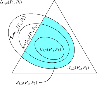
Figure 2: The geometry of various sets of distributions/tensors. We only draw sets of joint distributions/tensors. The geometry of the corresponding marginal distributions/tensors is similar. The ambient space is $\Delta_{1,2}(P_{1},P_{2})$ which is defined in Definition 12. The set ${\mathcal{J}}_{1,2}\left(P_{1},P_{2}\right)$ of self-couplings is defined in Definition 10. The set $\mathsf{Sym}_{1,2}(P_{1},P_{2})$ of symmetric tensors is defined in Definition 13. Inside $\mathsf{Sym}_{1,2}(P_{1},P_{2})$, there is a pair of dual cones, viz.: ${\mathcal{G}}_{{1,2}}\left(P_{1},P_{2}\right)$ (Definition 15) and $\mathrm{co}\text{-}{\mathcal{G}}_{1,2}\left(P_{1},P_{2}\right)$ (Definition 16). The blue region denotes the set ${\mathcal{S}}_{1,2}\left(P_{1},P_{2}\right)$ of symmetric distributions (Definition 14) which is the intersection of $\mathsf{Sym}_{1,2}(P_{1},P_{2})$ and ${\mathcal{J}}_{1,2}\left(P_{1},P_{2}\right)$.

Definition 12 (Generalized self-couplings).

$$\Delta_{1,2}(P_{1},P_{2})\coloneqq \left\{T_{{\mathbf{x}}^{1}_{1},{\mathbf{x}}^{1}_{2},{\mathbf{x}}^{2}_{1},{\mathbf{x}}^{2}_{2}}\in{\mathbb{R}}^{\left|{\mathcal{X}}_{1}\right|^{2}\times\left|{\mathcal{X}}_{2}\right|^{2}}:\left\|T_{{\mathbf{x}}^{1}_{1},{\mathbf{x}}^{1}_{2},{\mathbf{x}}^{2}_{1},{\mathbf{x}}^{2}_{2}}\right\|_{1}=1,\begin{array}[]{l}\left[T_{{\mathbf{x}}^{1}_{1},{\mathbf{x}}^{1}_{2},{\mathbf{x}}^{2}_{1},{\mathbf{x}}^{2}_{2}}\right]_{{\mathbf{x}}^{1}_{1}}=\left[T_{{\mathbf{x}}^{1}_{1},{\mathbf{x}}^{1}_{2},{\mathbf{x}}^{2}_{1},{\mathbf{x}}^{2}_{2}}\right]_{{\mathbf{x}}^{1}_{2}}=P_{1},\\ \left[T_{{\mathbf{x}}^{1}_{1},{\mathbf{x}}^{1}_{2},{\mathbf{x}}^{2}_{1},{\mathbf{x}}^{2}_{2}}\right]_{{\mathbf{x}}^{2}_{1}}=\left[T_{{\mathbf{x}}^{1}_{1},{\mathbf{x}}^{1}_{2},{\mathbf{x}}^{2}_{1},{\mathbf{x}}^{2}_{2}}\right]_{{\mathbf{x}}^{2}_{2}}=P_{2}\end{array}\right\},$$ (43)

$$\Delta_{1}(P_{1},P_{2})\coloneqq \left\{T_{{\mathbf{x}}^{1}_{1},{\mathbf{x}}^{1}_{2},{\mathbf{x}}^{2}}\in{\mathbb{R}}^{\left|{\mathcal{X}}_{1}\right|^{2}\times\left|{\mathcal{X}}_{2}\right|}:\left\|T_{{\mathbf{x}}^{1}_{1},{\mathbf{x}}^{1}_{2},{\mathbf{x}}^{2}}\right\|_{2}=1,\left[T_{{\mathbf{x}}^{1}_{1},{\mathbf{x}}^{1}_{2},{\mathbf{x}}^{2}}\right]_{{\mathbf{x}}^{1}_{1}}=\left[T_{{\mathbf{x}}^{1}_{1},{\mathbf{x}}^{1}_{2},{\mathbf{x}}^{2}}\right]_{{\mathbf{x}}^{1}_{2}}=P_{1},\left[T_{{\mathbf{x}}^{1}_{1},{\mathbf{x}}^{1}_{2},{\mathbf{x}}^{2}}\right]_{{\mathbf{x}}^{2}}=P_{2}\right\}$$

$$\Delta_{2}(P_{1},P_{2})\coloneqq \left\{T_{{\mathbf{x}}^{1},{\mathbf{x}}^{2}_{1},{\mathbf{x}}^{2}_{2}}\in{\mathbb{R}}^{\left|{\mathcal{X}}_{1}\right|\times\left|{\mathcal{X}}_{2}\right|^{2}}:\left\|T_{{\mathbf{x}}^{1},{\mathbf{x}}^{2}_{1},{\mathbf{x}}^{2}_{2}}\right\|_{2}=1,\left[T_{{\mathbf{x}}^{1},{\mathbf{x}}^{2}_{1},{\mathbf{x}}^{2}_{2}}\right]_{{\mathbf{x}}^{1}}=P_{1},\left[T_{{\mathbf{x}}^{1},{\mathbf{x}}^{2}_{1},{\mathbf{x}}^{2}_{2}}\right]_{{\mathbf{x}}^{2}_{1}}=\left[T_{{\mathbf{x}}^{1},{\mathbf{x}}^{2}_{1},{\mathbf{x}}^{2}_{2}}\right]_{{\mathbf{x}}^{2}_{2}}=P_{2}\right\}.$$

Remark 8.

For a general tensor (not necessarily a distribution) $T_{{\mathbf{a}},{\mathbf{b}}}\in{\mathbb{R}}^{\left|{\mathcal{A}}\right|\times\left|{\mathcal{B}}\right|}$, the marginalization of $T_{{\mathbf{a}},{\mathbf{b}}}$ onto the first variable ${\mathbf{a}}$ is defined as $\left[T_{{\mathbf{a}},{\mathbf{b}}}\right]_{{\mathbf{a}}}(a)\coloneqq\sum_{b\in{\mathcal{B}}}\left|T_{{\mathbf{a}},{\mathbf{b}}}(a,b)\right|$ for any $a\in{\mathcal{A}}$.

Remark 9.

For the convenience of discussion, the above sets should be thought of as generalizations of distributions (Definition 10).

Definition 13 (Symmetric tensors).

$$\mathsf{Sym}_{1,2}(P_{1},P_{2})\coloneqq \left\{T_{{\mathbf{x}}^{1}_{1},{\mathbf{x}}^{1}_{2},{\mathbf{x}}^{2}_{1},{\mathbf{x}}^{2}_{2}}\in\Delta_{1,2}(P_{1},P_{2}):T_{{\mathbf{x}}^{1}_{1},{\mathbf{x}}^{1}_{2},{\mathbf{x}}^{2}_{1},{\mathbf{x}}^{2}_{2}}=T_{{\mathbf{x}}^{1}_{2},{\mathbf{x}}^{1}_{1},{\mathbf{x}}^{2}_{2},{\mathbf{x}}^{2}_{1}}=T_{{\mathbf{x}}^{1}_{2},{\mathbf{x}}^{1}_{1},{\mathbf{x}}^{2}_{1},{\mathbf{x}}^{2}_{2}}=T_{{\mathbf{x}}^{1}_{1},{\mathbf{x}}^{1}_{2},{\mathbf{x}}^{2}_{2},{\mathbf{x}}^{2}_{1}}\right\},$$

$$\mathsf{Sym}_{1}(P_{1},P_{2})\coloneqq \left\{T_{{\mathbf{x}}^{1}_{1},{\mathbf{x}}^{1}_{2},{\mathbf{x}}^{2}}\in\Delta_{1}(P_{1},P_{2}):T_{{\mathbf{x}}^{1}_{1},{\mathbf{x}}^{1}_{2},{\mathbf{x}}^{2}}=T_{{\mathbf{x}}^{1}_{2},{\mathbf{x}}^{1}_{1},{\mathbf{x}}^{2}}\right\},$$

$$\mathsf{Sym}_{2}(P_{1},P_{2})\coloneqq \left\{T_{{\mathbf{x}}^{1},{\mathbf{x}}^{2}_{1},{\mathbf{x}}^{2}_{2}}\in\Delta_{2}(P_{1},P_{2}):T_{{\mathbf{x}}^{1},{\mathbf{x}}^{2}_{1},{\mathbf{x}}^{2}_{2}}=T_{{\mathbf{x}}^{1},{\mathbf{x}}^{2}_{2},{\mathbf{x}}^{2}_{1}}\right\}.$$

Definition 14 (Symmetric distributions).

$${\mathcal{S}}_{1,2}\left(P_{1},P_{2}\right)\coloneqq {\mathcal{J}}_{1,2}\left(P_{1},P_{2}\right)\cap\mathsf{Sym}_{1,2}(P_{1},P_{2}),$$

$${\mathcal{S}}_{1}\left(P_{1},P_{2}\right)\coloneqq {\mathcal{J}}_{1}\left(P_{1},P_{2}\right)\cap\mathsf{Sym}_{1}(P_{1},P_{2}),$$

$${\mathcal{S}}_{2}\left(P_{1},P_{2}\right)\coloneqq {\mathcal{J}}_{2}\left(P_{1},P_{2}\right)\cap\mathsf{Sym}_{2}(P_{1},P_{2}).$$

Definition 15 (Good distributions).

Let $(P_{1},P_{2})\in\Gamma_{1}\times\Gamma_{2}$. The set of jointly good distributions ${\mathcal{G}}_{{1,2}}\left(P_{1},P_{2}\right)$, the set of first marginally good distributions ${\mathcal{G}}_{{1}}\left(P_{1},P_{2}\right)$ and the set of second marginally good distributions ${\mathcal{G}}_{{2}}\left(P_{1},P_{2}\right)$ w.r.t. $P_{1}$ and $P_{2}$ are defined as follows:

$${\mathcal{G}}_{{1,2}}\left(P_{1},P_{2}\right)\coloneqq \left\{P_{{\mathbf{x}}^{1}_{1},{\mathbf{x}}^{1}_{2},{\mathbf{x}}^{2}_{1},{\mathbf{x}}^{2}_{2}}\in{\mathcal{J}}_{1,2}\left(P_{1},P_{2}\right)\colon\begin{array}[]{l}\exists k\in{\mathbb{Z}}_{\geq 1},\left\{\lambda_{i}\right\}_{i=1}^{k}\subseteq[0,1],\left\{P_{1,i}\right\}_{i=1}^{k}\subseteq\Delta({\mathcal{X}}_{1}),\left\{P_{2,i}\right\}_{i=1}^{k}\subseteq\Delta({\mathcal{X}}_{2}),\mathrm{\ s.t.}\\ \displaystyle\sum_{i=1}^{k}\lambda_{i}=1,P_{{\mathbf{x}}^{1}_{1},{\mathbf{x}}^{1}_{2},{\mathbf{x}}^{2}_{1},{\mathbf{x}}^{2}_{2}}=\sum_{i=1}^{k}\lambda_{i}P_{1,i}^{\otimes 2}\otimes P_{2,i}^{\otimes 2}\end{array}\right\},$$ (46)

$${\mathcal{G}}_{{1}}\left(P_{1},P_{2}\right)\coloneqq \left\{P_{{\mathbf{x}}^{1}_{1},{\mathbf{x}}^{1}_{2},{\mathbf{x}}^{2}}\in{\mathcal{J}}_{1}\left(P_{1},P_{2}\right)\colon\begin{array}[]{l}\exists k\in{\mathbb{Z}}_{\geq 1},\left\{\lambda_{i}\right\}_{i=1}^{k}\subseteq[0,1],\left\{P_{1,i}\right\}_{i=1}^{k}\subseteq\Delta({\mathcal{X}}_{1}),\left\{P_{2,i}\right\}_{i=1}^{k}\subseteq\Delta({\mathcal{X}}_{2}),\mathrm{\ s.t.}\\ \displaystyle\sum_{i=1}^{k}\lambda_{i}=1,P_{{\mathbf{x}}^{1}_{1},{\mathbf{x}}^{1}_{2},{\mathbf{x}}^{2}}=\sum_{i=1}^{k}\lambda_{i}P_{1,i}^{\otimes 2}\otimes P_{2,i}\end{array}\right\},$$ (49)

$${\mathcal{G}}_{{2}}\left(P_{1},P_{2}\right)\coloneqq \left\{P_{{\mathbf{x}}^{1},{\mathbf{x}}^{2}_{1},{\mathbf{x}}^{2}_{2}}\in{\mathcal{J}}_{2}\left(P_{1},P_{2}\right)\colon\begin{array}[]{l}\exists k\in{\mathbb{Z}}_{\geq 1},\left\{\lambda_{i}\right\}_{i=1}^{k}\subseteq[0,1],\left\{P_{1,i}\right\}_{i=1}^{k}\subseteq\Delta({\mathcal{X}}_{1}),\left\{P_{2,i}\right\}_{i=1}^{k}\subseteq\Delta({\mathcal{X}}_{2}),\mathrm{\ s.t.}\\ \displaystyle\sum_{i=1}^{k}\lambda_{i}=1,P_{{\mathbf{x}}^{1},{\mathbf{x}}^{2}_{1},{\mathbf{x}}^{2}_{2}}=\sum_{i=1}^{k}\lambda_{i}P_{1,i}\otimes P_{2,i}^{\otimes 2}\end{array}\right\}.$$ (52)

In addition, we define the set of simultaneously good distributions ${\mathcal{G}}\left(P_{1},P_{2}\right)$ w.r.t. $P_{1}$ and $P_{2}$ as

$${\mathcal{G}}\left(P_{1},P_{2}\right)\coloneqq \left\{\begin{array}[]{rl}P_{{\mathbf{x}}^{1}_{1},{\mathbf{x}}^{1}_{2},{\mathbf{x}}^{2}_{1},{\mathbf{x}}^{2}_{2}}\in{\mathcal{G}}_{{1,2}}\left(P_{1},P_{2}\right)\setminus{\mathcal{K}}_{{1,2}}\left(P_{1},P_{2}\right):&\\ \left[P_{{\mathbf{x}}^{1}_{1},{\mathbf{x}}^{1}_{2},{\mathbf{x}}^{2}_{1},{\mathbf{x}}^{2}_{2}}\right]_{{\mathbf{x}}^{1}_{1},{\mathbf{x}}^{1}_{2},{\mathbf{x}}^{2}_{1}}=&\left[P_{{\mathbf{x}}^{1}_{1},{\mathbf{x}}^{1}_{2},{\mathbf{x}}^{2}_{1},{\mathbf{x}}^{2}_{2}}\right]_{{\mathbf{x}}^{1}_{1},{\mathbf{x}}^{1}_{2},{\mathbf{x}}^{2}_{2}}\in{\mathcal{G}}_{{1}}\left(P_{1},P_{2}\right)\setminus{\mathcal{K}}_{{1}}\left(P_{1},P_{2}\right)\\ \left[P_{{\mathbf{x}}^{1}_{1},{\mathbf{x}}^{1}_{2},{\mathbf{x}}^{2}_{1},{\mathbf{x}}^{2}_{2}}\right]_{{\mathbf{x}}^{1}_{1},{\mathbf{x}}^{2}_{1},{\mathbf{x}}^{2}_{2}}=&\left[P_{{\mathbf{x}}^{1}_{1},{\mathbf{x}}^{1}_{2},{\mathbf{x}}^{2}_{1},{\mathbf{x}}^{2}_{2}}\right]_{{\mathbf{x}}^{1}_{2},{\mathbf{x}}^{2}_{1},{\mathbf{x}}^{2}_{2}}\in{\mathcal{G}}_{{2}}\left(P_{1},P_{2}\right)\setminus{\mathcal{K}}_{{2}}\left(P_{1},P_{2}\right)\end{array}\right\}.$$ (56)

Proposition 17 (Properties of good distributions).

The sets ${\mathcal{G}}_{{1}}\left(P_{1},P_{2}\right),{\mathcal{G}}_{{2}}\left(P_{1},P_{2}\right)$ and ${\mathcal{G}}_{{1,2}}\left(P_{1},P_{2}\right)$ enjoy the following properties.

1. Good distributions are symmetric.

   $${\mathcal{G}}_{{1,2}}\left(P_{1},P_{2}\right)\subset{\mathcal{S}}_{1,2}\left(P_{1},P_{2}\right),\quad{\mathcal{G}}_{{1}}\left(P_{1},P_{2}\right)\subset{\mathcal{S}}_{1}\left(P_{1},P_{2}\right),\quad{\mathcal{G}}_{{2}}\left(P_{1},P_{2}\right)\subset{\mathcal{S}}_{2}\left(P_{1},P_{2}\right).$$

2. For any $P_{{\mathbf{x}}^{1}_{1},{\mathbf{x}}^{1}_{2},{\mathbf{x}}^{2}_{1},{\mathbf{x}}^{2}_{2}}\in{\mathcal{G}}_{{1,2}}\left(P_{1},P_{2}\right)$,

   $$\left[P_{{\mathbf{x}}^{1}_{1},{\mathbf{x}}^{1}_{2},{\mathbf{x}}^{2}_{1},{\mathbf{x}}^{2}_{2}}\right]_{{\mathbf{x}}^{1}_{1},{\mathbf{x}}^{1}_{2},{\mathbf{x}}^{2}_{1}}= \left[P_{{\mathbf{x}}^{1}_{1},{\mathbf{x}}^{1}_{2},{\mathbf{x}}^{2}_{1},{\mathbf{x}}^{2}_{2}}\right]_{{\mathbf{x}}^{1}_{1},{\mathbf{x}}^{1}_{2},{\mathbf{x}}^{2}_{2}},\quad\left[P_{{\mathbf{x}}^{1}_{1},{\mathbf{x}}^{1}_{2},{\mathbf{x}}^{2}_{1},{\mathbf{x}}^{2}_{2}}\right]_{{\mathbf{x}}^{1}_{1},{\mathbf{x}}^{2}_{1},{\mathbf{x}}^{2}_{2}}=\left[P_{{\mathbf{x}}^{1}_{1},{\mathbf{x}}^{1}_{2},{\mathbf{x}}^{2}_{1},{\mathbf{x}}^{2}_{2}}\right]_{{\mathbf{x}}^{1}_{2},{\mathbf{x}}^{2}_{1},{\mathbf{x}}^{2}_{2}}.$$

3. The sets ${\mathcal{G}}_{{1}}\left(P_{1},P_{2}\right)$ and ${\mathcal{G}}_{{2}}\left(P_{1},P_{2}\right)$ are projections of the set ${\mathcal{G}}_{{1,2}}\left(P_{1},P_{2}\right)$.

   $${\mathcal{G}}_{{1}}\left(P_{1},P_{2}\right)= \left\{\left[P_{{\mathbf{x}}^{1}_{1},{\mathbf{x}}^{1}_{2},{\mathbf{x}}^{2}_{1},{\mathbf{x}}^{2}_{2}}\right]_{{\mathbf{x}}^{1}_{1},{\mathbf{x}}^{1}_{2},{\mathbf{x}}^{2}_{1}}:P_{{\mathbf{x}}^{1}_{1},{\mathbf{x}}^{1}_{2},{\mathbf{x}}^{2}_{1},{\mathbf{x}}^{2}_{2}}\in{\mathcal{G}}_{{1,2}}\left(P_{1},P_{2}\right)\right\},$$

   $${\mathcal{G}}_{{2}}\left(P_{1},P_{2}\right)= \left\{\left[P_{{\mathbf{x}}^{1}_{1},{\mathbf{x}}^{1}_{2},{\mathbf{x}}^{2}_{1},{\mathbf{x}}^{2}_{2}}\right]_{{\mathbf{x}}^{1}_{1},{\mathbf{x}}^{2}_{1},{\mathbf{x}}^{2}_{2}}:P_{{\mathbf{x}}^{1}_{1},{\mathbf{x}}^{1}_{2},{\mathbf{x}}^{2}_{1},{\mathbf{x}}^{2}_{2}}\in{\mathcal{G}}_{{1,2}}\left(P_{1},P_{2}\right)\right\}.$$

Remark 10.

Though the good sets ${\mathcal{G}}_{{1,2}}\left(P_{1},P_{2}\right),{\mathcal{G}}_{{1}}\left(P_{1},P_{2}\right),{\mathcal{G}}_{{2}}\left(P_{1},P_{2}\right)$ are consistent under projections (the third property of Proposition 17), the confusability sets ${\mathcal{K}}_{{1,2}}\left(P_{1},P_{2}\right),{\mathcal{K}}_{{1}}\left(P_{1},P_{2}\right),{\mathcal{K}}_{{2}}\left(P_{1},P_{2}\right)$ are not. Operationally, this is because $({\underline{x}}^{1}_{i_{1}},{\underline{x}}^{1}_{j_{1}})$ (or $({\underline{x}}^{1}_{i_{1}},{\underline{x}}^{2}_{j_{2}})$) and $({\underline{x}}^{1}_{i_{2}},{\underline{x}}^{2}_{j_{1}})$ (or $({\underline{x}}^{1}_{i_{2}},{\underline{x}}^{2}_{j_{2}})$) are not necessarily confusable even if $({\underline{x}}^{1}_{i_{1}},{\underline{x}}^{2}_{j_{1}})$ and $({\underline{x}}^{1}_{i_{2}},{\underline{x}}^{2}_{j_{2}})$ are (for $i_{1}\neq i_{2}$ and $j_{1}\neq j_{2}$). Therefore, even the second property of Proposition 17 is guaranteed to hold for $P_{{\mathbf{x}}^{1}_{1},{\mathbf{x}}^{1}_{2},{\mathbf{x}}^{2}_{1},{\mathbf{x}}^{2}_{2}}\in{\mathcal{K}}_{{1,2}}\left(P_{1},P_{2}\right)$, let alone the third one.

Definition 16 (Co-good tensors).

$$\mathrm{co}\text{-}{\mathcal{G}}_{1,2}\left(P_{1},P_{2}\right)\coloneqq \left\{P_{{\mathbf{x}}^{1}_{1},{\mathbf{x}}^{1}_{2},{\mathbf{x}}^{2}_{1},{\mathbf{x}}^{2}_{2}}\in\mathsf{Sym}_{1,2}(P_{1},P_{2})\colon\forall P_{{\mathbf{x}}^{1}}\in\Delta({\mathcal{X}}_{1}),\forall P_{{\mathbf{x}}^{2}}\in\Delta({\mathcal{X}}_{2}),\left\langle P_{{\mathbf{x}}^{1}}^{\otimes 2}\otimes P_{{\mathbf{x}}^{2}}^{\otimes 2},P_{{\mathbf{x}}^{1}_{1},{\mathbf{x}}^{1}_{2},{\mathbf{x}}^{2}_{1},{\mathbf{x}}^{2}_{2}}\right\rangle\geq 0\right\},$$

$$\mathrm{co}\text{-}{\mathcal{G}}_{1}\left(P_{1},P_{2}\right)\coloneqq \left\{P_{{\mathbf{x}}^{1}_{1},{\mathbf{x}}^{1}_{2},{\mathbf{x}}^{2}}\in\mathsf{Sym}_{1}(P_{1},P_{2})\colon\forall P_{{\mathbf{x}}^{1}}\in\Delta({\mathcal{X}}_{1}),\forall P_{{\mathbf{x}}^{2}}\in\Delta({\mathcal{X}}_{2}),\left\langle P_{{\mathbf{x}}^{1}}^{\otimes 2}\otimes P_{{\mathbf{x}}^{2}},P_{{\mathbf{x}}^{1}_{1},{\mathbf{x}}^{1}_{2},{\mathbf{x}}^{2}}\right\rangle\geq 0\right\},$$

$$\mathrm{co}\text{-}{\mathcal{G}}_{2}\left(P_{1},P_{2}\right)\coloneqq \left\{P_{{\mathbf{x}}^{1},{\mathbf{x}}^{2}_{1},{\mathbf{x}}^{2}_{2}}\in\mathsf{Sym}_{2}(P_{1},P_{2})\colon\forall P_{{\mathbf{x}}^{1}}\in\Delta({\mathcal{X}}_{1}),\forall P_{{\mathbf{x}}^{2}}\in\Delta({\mathcal{X}}_{2}),\left\langle P_{{\mathbf{x}}^{1}}\otimes P_{{\mathbf{x}}^{2}}^{\otimes 2},P_{{\mathbf{x}}^{1},{\mathbf{x}}^{2}_{1},{\mathbf{x}}^{2}_{2}}\right\rangle\geq 0\right\}.$$

Remark 11.

Note that co-good tensors are not necessarily distributions. They may have negative entries.

Remark 12.

It follows from definition that the sets of good distributions are subsets of the corresponding co-good distributions, i.e.,

$${\mathcal{G}}_{{1,2}}\left(P_{1},P_{2}\right)\subset\mathrm{co}\text{-}{\mathcal{G}}_{1,2}\left(P_{1},P_{2}\right),\quad{\mathcal{G}}_{{1}}\left(P_{1},P_{2}\right)\subset\mathrm{co}\text{-}{\mathcal{G}}_{1}\left(P_{1},P_{2}\right),\quad{\mathcal{G}}_{{2}}\left(P_{1},P_{2}\right)\subset\mathrm{co}\text{-}{\mathcal{G}}_{2}\left(P_{1},P_{2}\right).$$

Definition 17 (Dual cone).

The dual cone ${\mathcal{B}}^{*}$ of a cone ${\mathcal{B}}$ in a Hilbert space ${\mathcal{H}}$ is defined as ${\mathcal{B}}^{*}\coloneqq\left\{b^{\prime}\in{\mathcal{H}}:\forall b\in{\mathcal{B}},\;\left\langle b,b^{\prime}\right\rangle\geq 0\right\}$.

Theorem 18 (Duality).

The sets ${\mathcal{G}}_{{1,2}}\left(P_{1},P_{2}\right)$, ${\mathcal{G}}_{{1}}\left(P_{1},P_{2}\right)$ and ${\mathcal{G}}_{{2}}\left(P_{1},P_{2}\right)$ are all closed convex pointed cones with non-empty interior. Furthermore, the following duality relations hold. In $\mathsf{Sym}_{1,2}(P_{1},P_{2})$, ${\mathcal{G}}_{{1,2}}\left(P_{1},P_{2}\right)$ and $\mathrm{co}\text{-}{\mathcal{G}}_{1,2}\left(P_{1},P_{2}\right)$ are dual cones of each other. In $\mathsf{Sym}_{1}(P_{1},P_{2})$, ${\mathcal{G}}_{{1}}\left(P_{1},P_{2}\right)$ and $\mathrm{co}\text{-}{\mathcal{G}}_{1}\left(P_{1},P_{2}\right)$ are dual cones of each other. In $\mathsf{Sym}_{2}(P_{1},P_{2})$, ${\mathcal{G}}_{{2}}\left(P_{1},P_{2}\right)$ and $\mathrm{co}\text{-}{\mathcal{G}}_{2}\left(P_{1},P_{2}\right)$ are dual cones of each other.

Proof.

We first prove the duality relations. Intuitively, the duality follows since the extremal rays of ${\mathcal{G}}_{{1,2}}\left(P_{1},P_{2}\right)$ (or ${\mathcal{G}}_{{1}}\left(P_{1},P_{2}\right)$, ${\mathcal{G}}_{{2}}\left(P_{1},P_{2}\right)$ respectively) are distributions of the form $P_{{\mathbf{x}}^{1}}^{\otimes 2}\otimes P_{{\mathbf{x}}^{2}}^{\otimes 2}$ (or $P_{{\mathbf{x}}^{1}}^{\otimes 2}\otimes P_{{\mathbf{x}}^{2}}$, $P_{{\mathbf{x}}^{1}}\otimes P_{{\mathbf{x}}^{2}}^{\otimes 2}$ respectively). Indeed, it follows from Definition 15 that

$${\mathcal{G}}_{{1,2}}\left(P_{1},P_{2}\right)= \operatorname{conv}\left\{P_{{\mathbf{x}}^{1}}^{\otimes 2}\otimes P_{{\mathbf{x}}^{2}}^{\otimes 2}:P_{{\mathbf{x}}^{1}}\in\Delta({\mathcal{X}}_{1}),P_{{\mathbf{x}}^{2}}\in\Delta({\mathcal{X}}_{2})\right\}\cap{\mathcal{J}}_{1,2}\left(P_{1},P_{2}\right),$$

$${\mathcal{G}}_{{1}}\left(P_{1},P_{2}\right)= \operatorname{conv}\left\{P_{{\mathbf{x}}^{1}}^{\otimes 2}\otimes P_{{\mathbf{x}}^{2}}:P_{{\mathbf{x}}^{1}}\in\Delta({\mathcal{X}}_{1}),P_{{\mathbf{x}}^{2}}\in\Delta({\mathcal{X}}_{2})\right\}\cap{\mathcal{J}}_{1}\left(P_{1},P_{2}\right),$$

$${\mathcal{G}}_{{2}}\left(P_{1},P_{2}\right)= \operatorname{conv}\left\{P_{{\mathbf{x}}^{1}}\otimes P_{{\mathbf{x}}^{2}}^{\otimes 2}:P_{{\mathbf{x}}^{1}}\in\Delta({\mathcal{X}}_{1}),P_{{\mathbf{x}}^{2}}\in\Delta({\mathcal{X}}_{2})\right\}\cap{\mathcal{J}}_{2}\left(P_{1},P_{2}\right),$$

where $\operatorname{conv}\left\{\cdot\right\}$ denotes the convex hull of a set. Therefore, one can replace $P_{{\mathbf{x}}^{1}_{1},{\mathbf{x}}^{1}_{2},{\mathbf{x}}^{2}_{1},{\mathbf{x}}^{2}_{2}}\in{\mathcal{G}}_{{1,2}}\left(P_{1},P_{2}\right)$ (or $P_{{\mathbf{x}}^{1}_{1},{\mathbf{x}}^{1}_{2},{\mathbf{x}}^{2}}$, $P_{{\mathbf{x}}^{1},{\mathbf{x}}^{2}_{1},{\mathbf{x}}^{2}_{2}}$ respectively) in the definition of ${\mathcal{G}}_{{1,2}}\left(P_{1},P_{2}\right)^{*}$ (or ${\mathcal{G}}_{{1}}\left(P_{1},P_{2}\right)^{*}$, ${\mathcal{G}}_{{2}}\left(P_{1},P_{2}\right)^{*}$ respectively) below with $P_{{\mathbf{x}}^{1}}^{\otimes 2}\otimes P_{{\mathbf{x}}^{2}}^{\otimes 2}$ (or $P_{{\mathbf{x}}^{1}}^{\otimes 2}\otimes P_{{\mathbf{x}}^{2}}$, $P_{{\mathbf{x}}^{1}}\otimes P_{{\mathbf{x}}^{2}}^{\otimes 2}$ respectively).

$${\mathcal{G}}_{{1,2}}\left(P_{1},P_{2}\right)^{*}= \left\{Q_{{\mathbf{x}}^{1}_{1},{\mathbf{x}}^{1}_{2},{\mathbf{x}}^{2}_{1},{\mathbf{x}}^{2}_{2}}\in\mathsf{Sym}_{1,2}(P_{1},P_{2}):\forall P_{{\mathbf{x}}^{1}_{1},{\mathbf{x}}^{1}_{2},{\mathbf{x}}^{2}_{1},{\mathbf{x}}^{2}_{2}}\in{\mathcal{G}}_{{1,2}}\left(P_{1},P_{2}\right),\;\left\langle P_{{\mathbf{x}}^{1}_{1},{\mathbf{x}}^{1}_{2},{\mathbf{x}}^{2}_{1},{\mathbf{x}}^{2}_{2}},Q_{{\mathbf{x}}^{1}_{1},{\mathbf{x}}^{1}_{2},{\mathbf{x}}^{2}_{1},{\mathbf{x}}^{2}_{2}}\right\rangle\geq 0\right\},$$

$${\mathcal{G}}_{{1}}\left(P_{1},P_{2}\right)^{*}= \left\{Q_{{\mathbf{x}}^{1}_{1},{\mathbf{x}}^{1}_{2},{\mathbf{x}}^{2}}\in\mathsf{Sym}_{1}(P_{1},P_{2}):\forall P_{{\mathbf{x}}^{1}_{1},{\mathbf{x}}^{1}_{2},{\mathbf{x}}^{2}}\in{\mathcal{G}}_{{1}}\left(P_{1},P_{2}\right),\;\left\langle P_{{\mathbf{x}}^{1}_{1},{\mathbf{x}}^{1}_{2},{\mathbf{x}}^{2}},Q_{{\mathbf{x}}^{1}_{1},{\mathbf{x}}^{1}_{2},{\mathbf{x}}^{2}}\right\rangle\geq 0\right\},$$

$${\mathcal{G}}_{{2}}\left(P_{1},P_{2}\right)^{*}= \left\{Q_{{\mathbf{x}}^{1},{\mathbf{x}}^{2}_{1},{\mathbf{x}}^{2}_{2}}\in\mathsf{Sym}_{2}(P_{1},P_{2}):\forall P_{{\mathbf{x}}^{1},{\mathbf{x}}^{2}_{1},{\mathbf{x}}^{2}_{2}}\in{\mathcal{G}}_{{2}}\left(P_{1},P_{2}\right),\;\left\langle P_{{\mathbf{x}}^{1},{\mathbf{x}}^{2}_{1},{\mathbf{x}}^{2}_{2}},Q_{{\mathbf{x}}^{1},{\mathbf{x}}^{2}_{1},{\mathbf{x}}^{2}_{2}}\right\rangle\geq 0\right\}.$$

After the replacement, we get exactly ${\mathcal{G}}_{{1,2}}\left(P_{1},P_{2}\right)$ (or ${\mathcal{G}}_{{1}}\left(P_{1},P_{2}\right)$, ${\mathcal{G}}_{{2}}\left(P_{1},P_{2}\right)$, respectively).

To formalize this intuition, we prove two-sided set inclusions for $\mathrm{co}\text{-}{\mathcal{G}}_{1,2}\left(P_{1},P_{2}\right)$ and $\mathrm{co}\text{-}{\mathcal{G}}_{1}\left(P_{1},P_{2}\right)$. The proof for $\mathrm{co}\text{-}{\mathcal{G}}_{2}\left(P_{1},P_{2}\right)$ is the same as that for $\mathrm{co}\text{-}{\mathcal{G}}_{1}\left(P_{1},P_{2}\right)$ up to change of notation.

We first prove $\mathrm{co}\text{-}{\mathcal{G}}_{1,2}\left(P_{1},P_{2}\right)={\mathcal{G}}_{{1,2}}\left(P_{1},P_{2}\right)^{*}$.

1. Let $Q_{{\mathbf{x}}^{1}_{1},{\mathbf{x}}^{1}_{2},{\mathbf{x}}^{2}_{1},{\mathbf{x}}^{2}_{2}}\in\mathrm{co}\text{-}{\mathcal{G}}_{1,2}\left(P_{1},P_{2}\right)$. Let $P_{{\mathbf{x}}^{1}_{1},{\mathbf{x}}^{1}_{2},{\mathbf{x}}^{2}_{1},{\mathbf{x}}^{2}_{2}}=\sum_{i=1}^{k}\lambda_{i}P_{1,i}^{\otimes 2}\otimes P_{2,i}^{\otimes 2}\in{\mathcal{G}}_{{1,2}}\left(P_{1},P_{2}\right)$. By Definition 16, we have $\left\langle Q_{{\mathbf{x}}^{1}_{1},{\mathbf{x}}^{1}_{2},{\mathbf{x}}^{2}_{1},{\mathbf{x}}^{2}_{2}},P_{1,i}^{\otimes 2}\otimes P_{2,i}^{\otimes 2}\right\rangle\geq 0$ for all $i\in[k]$. Therefore, $\left\langle P_{{\mathbf{x}}^{1}_{1},{\mathbf{x}}^{1}_{2},{\mathbf{x}}^{2}_{1},{\mathbf{x}}^{2}_{2}},Q_{{\mathbf{x}}^{1}_{1},{\mathbf{x}}^{1}_{2},{\mathbf{x}}^{2}_{1},{\mathbf{x}}^{2}_{2}}\right\rangle\geq 0$, which means $Q_{{\mathbf{x}}^{1}_{1},{\mathbf{x}}^{1}_{2},{\mathbf{x}}^{2}_{1},{\mathbf{x}}^{2}_{2}}\in{\mathcal{G}}_{{1,2}}\left(P_{1},P_{2}\right)^{*}$. This proves $\mathrm{co}\text{-}{\mathcal{G}}_{1,2}\left(P_{1},P_{2}\right)\subseteq{\mathcal{G}}_{{1,2}}\left(P_{1},P_{2}\right)^{*}$.

2. Let $Q_{{\mathbf{x}}^{1}_{1},{\mathbf{x}}^{1}_{2},{\mathbf{x}}^{2}_{1},{\mathbf{x}}^{2}_{2}}\in{\mathcal{G}}_{{1,2}}\left(P_{1},P_{2}\right)^{*}$. By Definition 17, for any $P_{{\mathbf{x}}^{1}}\in\Delta({\mathcal{X}}_{1})$ and $P_{{\mathbf{x}}^{2}}\in\Delta({\mathcal{X}}_{2})$, we have $\left\langle Q_{{\mathbf{x}}^{1}_{1},{\mathbf{x}}^{1}_{2},{\mathbf{x}}^{2}_{1},{\mathbf{x}}^{2}_{2}},P_{{\mathbf{x}}^{1}}^{\otimes 2}\otimes P_{{\mathbf{x}}^{2}}^{\otimes 2}\right\rangle\geq 0$ since $P_{{\mathbf{x}}^{1}}^{\otimes 2}\otimes P_{{\mathbf{x}}^{2}}^{\otimes 2}\in{\mathcal{G}}_{{1,2}}\left(P_{1},P_{2}\right)$. Therefore, $Q_{{\mathbf{x}}^{1}_{1},{\mathbf{x}}^{1}_{2},{\mathbf{x}}^{2}_{1},{\mathbf{x}}^{2}_{2}}\in\mathrm{co}\text{-}{\mathcal{G}}_{1,2}\left(P_{1},P_{2}\right)$ and ${\mathcal{G}}_{{1,2}}\left(P_{1},P_{2}\right)^{*}\subseteq\mathrm{co}\text{-}{\mathcal{G}}_{1,2}\left(P_{1},P_{2}\right)$.

We then prove $\mathrm{co}\text{-}{\mathcal{G}}_{1}\left(P_{1},P_{2}\right)={\mathcal{G}}_{{1}}\left(P_{1},P_{2}\right)^{*}$ in the same way.

1. Let $Q_{{\mathbf{x}}^{1}_{1},{\mathbf{x}}^{1}_{2},{\mathbf{x}}^{2}}\in\mathrm{co}\text{-}{\mathcal{G}}_{1,2}\left(P_{1},P_{2}\right)$. Let $P_{{\mathbf{x}}^{1}_{1},{\mathbf{x}}^{1}_{2},{\mathbf{x}}^{2}}=\sum_{i=1}^{k}\lambda_{i}P_{1,i}^{\otimes 2}\otimes P_{2,i}\in{\mathcal{G}}_{{1,2}}\left(P_{1},P_{2}\right)$. By Definition 16, for each $i\in[k]$, we have $\left\langle Q_{{\mathbf{x}}^{1}_{1},{\mathbf{x}}^{1}_{2},{\mathbf{x}}^{2}},P_{1,i}^{\otimes 2}\otimes P_{2,i}\right\rangle\geq 0$. Therefore, $\left\langle P_{{\mathbf{x}}^{1}_{1},{\mathbf{x}}^{1}_{2},{\mathbf{x}}^{2}},Q_{{\mathbf{x}}^{1}_{1},{\mathbf{x}}^{1}_{2},{\mathbf{x}}^{2}}\right\rangle\geq 0$, which means $Q_{{\mathbf{x}}^{1}_{1},{\mathbf{x}}^{1}_{2},{\mathbf{x}}^{2}}\in{\mathcal{G}}_{{1}}\left(P_{1},P_{2}\right)^{*}$. This proves $\mathrm{co}\text{-}{\mathcal{G}}_{1}\left(P_{1},P_{2}\right)\subseteq{\mathcal{G}}_{{1}}\left(P_{1},P_{2}\right)^{*}$.

2. Let $Q_{{\mathbf{x}}^{1}_{1},{\mathbf{x}}^{1}_{2},{\mathbf{x}}^{2}}\in{\mathcal{G}}_{{1}}\left(P_{1},P_{2}\right)^{*}$. By Definition 17, for any $P_{{\mathbf{x}}^{1}}\in\Delta({\mathcal{X}}_{1})$ and $P_{{\mathbf{x}}^{2}}\in\Delta({\mathcal{X}}_{2})$, we have $\left\langle Q_{{\mathbf{x}}^{1}_{1},{\mathbf{x}}^{1}_{2},{\mathbf{x}}^{2}},P_{{\mathbf{x}}^{1}}^{\otimes 2}\otimes P_{{\mathbf{x}}^{2}}\right\rangle\geq 0$ since $P_{{\mathbf{x}}^{1}}^{\otimes 2}\otimes P_{{\mathbf{x}}^{2}}\in{\mathcal{G}}_{{1}}\left(P_{1},P_{2}\right)$. Therefore, $Q_{{\mathbf{x}}^{1}_{1},{\mathbf{x}}^{1}_{2},{\mathbf{x}}^{2}}\in\mathrm{co}\text{-}{\mathcal{G}}_{1}\left(P_{1},P_{2}\right)$ and ${\mathcal{G}}_{{1}}\left(P_{1},P_{2}\right)^{*}\subseteq\mathrm{co}\text{-}{\mathcal{G}}_{1,2}\left(P_{1},P_{2}\right)$.

This finishes the proof for duality.

The claimed convexity and conic property of $\mathrm{co}\text{-}{\mathcal{G}}_{1,2}\left(P_{1},P_{2}\right)$, $\mathrm{co}\text{-}{\mathcal{G}}_{1}\left(P_{1},P_{2}\right)$ and $\mathrm{co}\text{-}{\mathcal{G}}_{2}\left(P_{1},P_{2}\right)$ follow directly from Definition 16. The closedness of ${\mathcal{G}}_{{1,2}}\left(P_{1},P_{2}\right)$, ${\mathcal{G}}_{{1}}\left(P_{1},P_{2}\right)$ and ${\mathcal{G}}_{{2}}\left(P_{1},P_{2}\right)$ follows from the fact that the dual cone of any convex cone is closed. One can easily find distributions that are in the interior of the cones under consideration. The pointedness of ${\mathcal{G}}_{{1,2}}\left(P_{1},P_{2}\right)$, ${\mathcal{G}}_{{1}}\left(P_{1},P_{2}\right)$ and ${\mathcal{G}}_{{2}}\left(P_{1},P_{2}\right)$ follows from nonnegativity of the entries of their elements. Finally, the pointedness of $\mathrm{co}\text{-}{\mathcal{G}}_{1,2}\left(P_{1},P_{2}\right)$, $\mathrm{co}\text{-}{\mathcal{G}}_{1}\left(P_{1},P_{2}\right)$ and $\mathrm{co}\text{-}{\mathcal{G}}_{2}\left(P_{1},P_{2}\right)$ follows from the fact that the dual cone of any convex cone with nonempty interior is pointed. ∎

XI A characterization of the shape of capacity region

Theorem 19.

Fix a pair of input distributions $(P_{1},P_{2})\in\Gamma_{1}\times\Gamma_{2}$.

1. If ${\mathcal{G}}\left(P_{1},P_{2}\right)\neq\emptyset$, then the capacity region contains rate pairs $(R_{1},R_{2})$ such that $R_{1}>0,R_{2}>0$ or $R_{1}>0,R_{2}=0$ or $R_{1}=0,R_{2}>0$ or $R_{1}=0,R_{2}=0$.

2. If ${\mathcal{G}}\left(P_{1},P_{2}\right)=\emptyset$, ${\mathcal{G}}_{{1}}\left(P_{1},P_{2}\right)\setminus{\mathcal{K}}_{{1}}\left(P_{1},P_{2}\right)\neq\emptyset$ and ${\mathcal{G}}_{{2}}\left(P_{1},P_{2}\right)\setminus{\mathcal{K}}_{{2}}\left(P_{1},P_{2}\right)\neq\emptyset$, then the capacity region only contains rate pairs $(R_{1},R_{2})$ such that $R_{1}>0,R_{2}=0$ or $R_{1}=0,R_{2}>0$ or $R_{1}=0,R_{2}=0$.

3. If ${\mathcal{G}}_{{1}}\left(P_{1},P_{2}\right)\setminus{\mathcal{K}}_{{1}}\left(P_{1},P_{2}\right)\neq\emptyset$ and ${\mathcal{G}}_{{1}}\left(P_{1},P_{2}\right)\setminus{\mathcal{K}}_{{2}}\left(P_{1},P_{2}\right)=\emptyset$, then the capacity region only contains rate pairs $(R_{1},R_{2})$ such that $R_{1}>0,R_{2}=0$ or $R_{1}=0,R_{2}=0$.

4. If ${\mathcal{G}}_{{1}}\left(P_{1},P_{2}\right)\setminus{\mathcal{K}}_{{1}}\left(P_{1},P_{2}\right)=\emptyset$ and ${\mathcal{G}}_{{1}}\left(P_{1},P_{2}\right)\setminus{\mathcal{K}}_{{2}}\left(P_{1},P_{2}\right)\neq\emptyset$, then the capacity region only contains rate pairs $(R_{1},R_{2})$ such that $R_{1}=0,R_{2}>0$ or $R_{1}=0,R_{2}=0$.

5. If ${\mathcal{G}}_{{1}}\left(P_{1},P_{2}\right)\setminus{\mathcal{K}}_{{1}}\left(P_{1},P_{2}\right)=\emptyset$ and ${\mathcal{G}}_{{1}}\left(P_{1},P_{2}\right)\setminus{\mathcal{K}}_{{2}}\left(P_{1},P_{2}\right)=\emptyset$, then the capacity region only contains $(0,0)$.

Cases	${\mathcal{G}}\left(P_{1},P_{2}\right)\neq\emptyset$	${\mathcal{G}}_{{1}}\left(P_{1},P_{2}\right)\setminus{\mathcal{K}}_{{1}}\left(P_{1},P_{2}\right)\neq\emptyset$	${\mathcal{G}}_{{2}}\left(P_{1},P_{2}\right)\setminus{\mathcal{K}}_{{2}}\left(P_{1},P_{2}\right)\neq\emptyset$	Capacity region
Case (1)	$\checkmark$	$\checkmark$	$\checkmark$	$(+,+),(+,0),(0,+),(0,0)$
Case (2)	$\times$	$\checkmark$	$\checkmark$	$(+,0),(0,+),(0,0)$
Case (3)	$\times$	$\checkmark$	$\times$	$(+,0),(0,0)$
Case (4)	$\times$	$\times$	$\checkmark$	$(0,+),(0,0)$
Case (5)	$\times$	$\times$	$\times$	$(0,0)$

TABLE I: A characterization of the shape of the capacity region of any omniscient adversarial two-user MAC. Note that the condition ${\mathcal{G}}\left(P_{1},P_{2}\right)\neq\emptyset$ implies both ${\mathcal{G}}_{{1}}\left(P_{1},P_{2}\right)\setminus{\mathcal{K}}_{{1}}\left(P_{1},P_{2}\right)\neq\emptyset$ and ${\mathcal{G}}_{{2}}\left(P_{1},P_{2}\right)\setminus{\mathcal{K}}_{{2}}\left(P_{1},P_{2}\right)\neq\emptyset$. Indeed, the former condition is strictly stronger. In each case, we highlight the conditions in colors in such a way that red conditions imply blue conditions. Note that the table above covers all possible cases.

The proof of the above characterization is comprised of two parts: achievability (Lemma 23) and converse (Theorem 20).

Theorem (Achievability, restatement of Lemma 23).

Fix input distributions $(P_{1},P_{2})\in\Gamma_{1}\times\Gamma_{2}$.

1. If ${\mathcal{G}}\left(P_{1},P_{2}\right)\neq\emptyset$, then there exist achievable rate pairs $(R_{1},R_{2})$ such that $R_{1}>0,R_{2}>0$.

2. If ${\mathcal{G}}_{{1}}\left(P_{1},P_{2}\right)\setminus{\mathcal{K}}_{{1}}\left(P_{1},P_{2}\right)\neq\emptyset$, then there exist achievable rate pairs $(R_{1},0)$ such that $R_{1}>0$.

3. If ${\mathcal{G}}_{{2}}\left(P_{1},P_{2}\right)\setminus{\mathcal{K}}_{{2}}\left(P_{1},P_{2}\right)\neq\emptyset$, then there exist achievable rate pairs $(0,R_{2})$ such that $R_{2}>0$.

Various achievability results are proved in Section XIII. Firstly, in Lemma 22, we prove the existence of positive rates using product distributions. Next, in Lemma 23, we refine this result using mixtures of product distributions, i.e., good distributions (Definition 15). Finally, in Lemma 24 we present inner bounds on the capacity region using product distributions.

Theorem 20 (Converse).

Fix a pair of input distributions $(P_{1},P_{2})\in\Gamma_{1}\times\Gamma_{2}$.

1. If ${\mathcal{G}}\left(P_{1},P_{2}\right)=\emptyset$, then there does not exist achievable rate pair $(R_{1},R_{2})$ such that $R_{1}>0,R_{2}>0$.

2. If ${\mathcal{G}}_{{1}}\left(P_{1},P_{2}\right)\setminus{\mathcal{K}}_{{1}}\left(P_{1},P_{2}\right)=\emptyset$, then there does not exist achievable rate pair $(R_{1},R_{2})$ such that $R_{1}>0$.

3. If ${\mathcal{G}}_{{2}}\left(P_{1},P_{2}\right)\setminus{\mathcal{K}}_{{2}}\left(P_{1},P_{2}\right)=\emptyset$, then there does not exist achievable rate pair $(R_{1},R_{2})$ such that $R_{2}>0$.

Proof.

Item 1 is proved in Section XIV. Items 2 and 3 are proved in Section XV. ∎

Observation 13.

For an omniscient two-user adversarial MAC, for $i=1,2$, if a rate $R_{i}>0$ is achievable for transmitter $i$, then any rate $0\leq R_{i}^{\prime}\leq R_{i}$ is also achievable for transmitter $i$.

By 13, if the capacity region contains a rate pair $(R_{1},R_{2})$ where $R_{1}>0,R_{2}>0$, then the rate pairs $(R_{1},0)$ and $(0,R_{2})$ are also in the capacity region.

XI-A A remark on nonconvexity of capacity region

As suggested by Theorem 19, the capacity region of an adversarial MAC can be nonconvex. E.g., if a MAC satisfies the conditions in Item 2 of Theorem 19, then the capacity region only consists of two perpendicular line segments and is therefore nonconvex. However, the capacity region cannot be an arbitrary nonconvex region. Indeed, 13 implies that if a rate pair $(R_{1},R_{2})$ with $R_{1}>0,R_{2}>0$ is achievable, then all rate pairs in the (closed) rectangle with vertices $(0,0),(R_{1},0),(0,R_{2}),(R_{1},R_{2})$ are also achievable.

For AVMACs (i.e., the oblivious adversarial MACs), the nonconvexity of the capacity region was noted by Gubner–Hughes [GH95] and Pereg–Steinberg [PS19] via the example of an (oblivious) erasure MAC. As a side note, for AVMACs equipped with common randomness, the capacity region may or may not be convex, depending on how the common randomness is instantiated. If each encoder shares an independent secret key with the decoder, then the corresponding capacity region, known as the divided-randomness capacity region, is not necessarily convex [GH95]. On the other hand, if all of two encoders and the decoder share the same key, then the corresponding capacity region, known as the random code capacity region, is always convex [PS19]. In our work, we do not equip any party with shared randomness. See [PS19] for a more detailed discussion on the nonconvexity of the capacity region of AVMACs.

XI-B Comparison of our results with [PS19] on (oblivious) AVMACs

We compare below our results with the parallel results by Pereg and Steinberg on oblivious AVMACs. For simplicity, we only compare the characterizations of positivity of capacities. Specifically, an oblivious AVMAC is a general adversarial MAC with input and state constraints and an oblivious adversary who does not know the transmitted sequences from any of the encoders. As many other results in the AVC literature, their characterization involves the oblivious analog of confusability known as symmetrizability. Proper notions of first marginal symmetrizability, second marginal symmetrizability and joint symmetrizability (denoted in their notation by symmetrizability-${\mathcal{X}}_{1}|{\mathcal{X}}_{2}$, symmetrizability-${\mathcal{X}}_{2}|{\mathcal{X}}_{1}$ and symmetrizability-${\mathcal{X}}_{1}\times{\mathcal{X}}_{2}$ respectively) were introduced and were shown to characterize the capacity positivity. See Table II below.

Cases	non-joint symmetrizability	non-first marginal symmetrizability	non-second marginal symmetrizability	Capacity region
Case (1)	$\checkmark$	$\checkmark$	$\checkmark$	$(+,+),(+,0),(0,+),(0,0)$
Case (2)	$\checkmark$	$\checkmark$	$\times$	$(+,0),(0,0)$
Case (3)	$\checkmark$	$\times$	$\checkmark$	$(0,+),(0,0)$
Case (4)	$\times$	$?$	$?$	$(0,0)$
Case (5)	$\checkmark$	$\times$	$\times$	$(0,0)$

TABLE II: Results in [PS19] on capacity positivity of oblivious AVMACs. In the table, “$\checkmark$” (resp. “$\times$”) means the corresponding non-symmetrizability condition is satisfied (resp. unsatisfied). Question marks “$?$” mean either satisfied or unsatisfied, regardlessly. As noted, non-joint symmetrizability is a necessary condition for any positive achievable rate.

Intuitively, one should think of symmetrizability as the oblivious analog of confusability defined in Section IX. However, in the AVMAC setting, due to the “independence” between the jammer and the encoders, the formal definition of symmetrizability does not appear to be a straightforward adjustment of Definition 11. As a result, the characterization of positivity in [PS19] does not exactly parallel ours. An informal analogy between the symmetrizability of Pereg and Steinberg’s and the confusability of ours is as follows. Non-first (resp. -second) marginal symmetrizability corresponds to ${\mathcal{G}}_{{1}}\left(P_{1},P_{2}\right)\setminus{\mathcal{K}}_{{1}}\left(P_{1},P_{2}\right)\neq\emptyset$ (resp. ${\mathcal{G}}_{{2}}\left(P_{1},P_{2}\right)\setminus{\mathcal{K}}_{{2}}\left(P_{1},P_{2}\right)\neq\emptyset$). Non-joint symmetrizability corresponds to ${\mathcal{G}}_{{1,2}}\left(P_{1},P_{2}\right)\setminus{\mathcal{K}}_{{1,2}}\left(P_{1},P_{2}\right)\neq\emptyset$. However, one gets wrong results (for Items 1 and 2 in particular) if she/he verbatim translates the oblivious results to the omniscient setting using the aforementioned informal correspondence.

In the AVMAC setting, non-joint symmetrizability is a necessary condition for the existence of $R_{1}>0$ or $R_{2}>0$. As a consequence, there does not exist situation where $R_{1}>0$ or $R_{2}>0$ can be achieved separately yet not simultaneously (Item 2 in Theorem 19).

In the omniscient setting, the condition that determines the possibility of $(R_{1},R_{2})$ with $R_{1}>0,R_{2}>0$ is in terms of ${\mathcal{G}}\left(P_{1},P_{2}\right)$ rather than ${\mathcal{G}}_{{1,2}}\left(P_{1},P_{2}\right)\setminus{\mathcal{K}}_{{1,2}}\left(P_{1},P_{2}\right)$. Communication at positive rates for both encoders simultaneously may not be possible even if ${\mathcal{G}}_{{1,2}}\left(P_{1},P_{2}\right)\setminus{\mathcal{K}}_{{1,2}}\left(P_{1},P_{2}\right)\neq\emptyset$. It is possible only if there is a single good distribution (as per Definition 15) that is simultaneously non-jointly symmetrizable and non-marginally symmetrizable (for both transmitters).

XII Overview of proof techniques

In this section we overview the proof techniques for establishing Theorem 19. Since there are cases where both/exactly one/none of the transmitters can achieve positive rates, we have to divide the analysis into several cases. Nevertheless, the proofs for different cases share roughly the same structure. In what follows, we briefly introduce the ideas behind the achievability part and the converse part separately.

XII-A Proof techniques for achievability

To show positive achievable rates under the conditions of Lemma 23, we use the standard method of random coding with expurgation. The conditions in Lemma 23 can be intuitively interpreted as the existence of good distributions (according to Definition 15) that are not bad (according to Definition 11).

If one is able to find a product distribution (which is always good by definition) that is outside the confusability sets, then one can simply sample positive rate codes whose entries are i.i.d. according to the distribution. By concentration of measure, the joint type of any codeword tuple is tightly concentrated around the product distribution. In particular, any joint type is outside the confusability sets with high probability. Now by large deviation principle, if the code rates are sufficiently small, a union bound over all codeword tuples allows us to conclude that no joint type is confusable and hence the whole code pair attains zero error with high probability. This gives Lemma 22.

Lemma 22 can be strengthened in the following two ways.

Firstly, even if product distributions are confusable, if one can find mixtures of product distributions that are outside the confusability sets, then positive rates are still achievable. Here the additional idea is time-sharing. Recall that a good distribution is a convex combination of product distributions. The coefficients of the convex combination can be regarded as giving a time-sharing sequence. We then sample random codes in the following way. All codewords are chopped up into chunks of lengths proportional to the convex combination coefficients. Entries of all codewords in a particular chunk are i.i.d. according the corresponding component distribution of the convex combination. Effectively it is as if we convexly concatenate multiple codebooks of shorter lengths sampled from different product distributions. Again by a Chernoff-union argument, all joint types are tightly concentrated around the mixture distribution provided that the rates are sufficiently small. Since the mixture distribution itself is outside the confusability sets, the code pair attains zero error with high probability. This gives Lemma 23. Such a code construction is known as coded time-sharing (see Remark 14).

Secondly, by carefully analyzing the large deviation exponent, one can in fact obtain inner bounds on the capacity region. To this end, one could not simply set the rates to be sufficiently small so as to admit a union bound. A standard trick is to remove (a.k.a. expurgate) one codeword from each confusable pair. Using Sanov’s theorem (Lemma 3), one can get the exact exponent of the probability of sampling a confusable pair. One can then set the rates so as to guarantee that the (expected) number of expurgated codewords is at most, say, half of the code size. This ensures that the expurgation process does not hurt the rate. This gives Lemma 24. We remark that if one wishes to achieve a rate pair with two positive rates, then the above argument requires one to expurgate codewords that contribute to (at least one of) jointly confusable pairs, first marginally confusable pairs or second marginally confusable pairs. We believe that such an expurgation strategy is pessimistic and higher rates may be obtained using more clever expurgation strategies. See Item 4 in Section XVI.

XII-B Proof techniques for converse

The converse part is considerably more involved. At a high level, it is inspired by the classical Plotkin bound in coding theory and follows a similar structure as [WBBJ19]. However, due to the multiuser nature of the channel, the case analysis is more delicate.

The basic proof strategy is comprised of the following components. Given any code pair $({\mathcal{C}}_{1},{\mathcal{C}}_{2})$ that attains zero error, we would like to show that they have zero rate(s) once the conditions in Theorem 20 are satisfied. To this end, we follow the steps below.

1. First, we extract a subcode pair $({\mathcal{C}}_{1}^{\prime},{\mathcal{C}}_{2}^{\prime})$ which has nontrivial sizes and is “equicoupled”. More specifically, for one thing, the code sizes are mildly large in the sense that $|{\mathcal{C}}_{i}^{\prime}|\xrightarrow{|{\mathcal{C}}_{i}|\to\infty}\infty$ for $i=1,2$. In fact $|{\mathcal{C}}_{i}^{\prime}|=f(|{\mathcal{C}}_{i}|)$ where $f(\cdot)$ is the inverse Ramsey number which grows extremely slow. However, this is enough for our purposes since it will be ultimately proved that $\max\left\{|{\mathcal{C}}_{1}^{\prime}|,|{\mathcal{C}}^{\prime}|\right\}\leq C$ for some constant $C>0$ independent of $n$. Then $\max\left\{|{\mathcal{C}}_{1}|,|{\mathcal{C}}_{2}|\right\}\leq f^{-1}(C)$ which is a huge constant. However, this is already more than sufficient to imply zero rates. For another (more important) thing, the subcode pair we obtained is highly structured in the sense that the joint type of any codeword tuple from the subcode pair is approximately the same (hence the subcodes are at times called equicoupled in this paper). This follows from Ramsey’s theorem (Theorem 26). At the cost of losing rates (which is actually fine), we localize some highly regular structures into a tiny subcode pair.

2. We then focus on the subcode pair. It is unclear whether or not the distribution that all joint types are concentrated around is symmetric (as per Definition 14). However, viewing the codebook as a sequence of random variables, we can show (in Section XIV-B) that the size of the equicoupled subcode must be small if the distribution is asymmetric. This, after some preprocessing of the sequence of random variables, follows from a classical theorem by Komlós (Theorem 29).

3. Now we assume that the equicoupled subcode is equipped with a symmetric distribution. Since we started with a code pair of zero error, all joint types are outside the confusability sets. Hence by the equicoupledness property, the associated distribution is outside the confusability sets as well. By the assumptions of Theorem 20, this distribution cannot be good (as per Definition 15) since the sets of good distributions are assumed to be subsets of the confusability sets. By the duality (Theorem 18) between the sets of good and “co-good” tensors (Definition 16), we can find a witness (which itself is a co-good tensor) of the non-goodness of the distribution. This finally allows us to apply a Plotkin-type double counting trick. Specifically, we upper and lower bound the following crucial quantity (Equation 96): the average inner product between the witness and the joint types in the subcodes. Careful calculations give us upper and lower bounds on this quantity. Contrasting these bounds further gives us an upper bound on the code sizes as promised.

Similar argument can be adapted to the marginal case where exactly one transmitter suffers from zero capacity.

XIII Achievability

We need the following lemma which concentrates the size of the constant composition component of a random code. The proof follows from the Chernoff bound (Lemma 2) and can be found in, e.g., [ZBJ20].

Lemma 21.

Let ${\mathcal{C}}\subseteq{\mathcal{X}}^{n}$ be a random code that consists of codewords ${\underline{\mathbf{x}}}_{1},\cdots,{\underline{\mathbf{x}}}_{M}$ i.i.d. according to $P_{\mathbf{x}}^{\otimes n}$ for some $P_{\mathbf{x}}\in\Delta({\mathcal{X}})$. Let ${\mathcal{C}}^{\prime}\subseteq{\mathcal{C}}$ be the $P_{\mathbf{x}}$-constant composition subcode of ${\mathcal{C}}$. Then

$$\Pr\left[\left|{\mathcal{C}}^{\prime}\right|\notin(1\pm 1/2)\frac{M}{\nu(P_{\mathbf{x}},n)}\right]\leq 2\exp\left(-\frac{M}{12\nu(P_{\mathbf{x}},n)}\right).$$

XIII-A Positive achievable rates via product distributions

Lemma 22 (Positive achievable rates via product distributions).

Let $(P_{1},P_{2})\in\Gamma_{1}\times\Gamma_{2}$.

1. If $P_{1}^{\otimes 2}\otimes P_{2}^{\otimes 2}\notin{\mathcal{K}}_{{1,2}}\left(P_{1},P_{2}\right)$, $P_{1}^{\otimes 2}\otimes P_{2}\notin{\mathcal{K}}_{{1}}\left(P_{1},P_{2}\right)$ and $P_{1}\otimes P_{2}^{\otimes 2}\notin{\mathcal{K}}_{{2}}\left(P_{1},P_{2}\right)$, then there exist achievable rate pairs $(R_{1},R_{2})$ such that $R_{1}>0,R_{2}>0$.

2. If $P_{1}^{\otimes 2}\otimes P_{2}\notin{\mathcal{K}}_{{1}}\left(P_{1},P_{2}\right)$, then there exist achievable rate pairs $(R_{1},R_{2})$ such that $R_{1}>0,R_{2}=0$.

3. If $P_{1}\otimes P_{2}^{\otimes 2}\notin{\mathcal{K}}_{{1}}\left(P_{1},P_{2}\right)$, then there exist achievable rate pairs $(R_{1},R_{2})$ such that $R_{1}=0,R_{2}>0$.

Proof of Item 1 in Lemma 22.

Assume that both $P_{1}$ and $P_{2}$ have no zero atoms. Sample a random code pair $\left({\mathcal{C}}_{1},{\mathcal{C}}_{2}\right)\subseteq{\mathcal{X}}_{1}^{n}\times{\mathcal{X}}_{2}^{n}$ of sizes $(M_{1},M_{2})$, where ${\mathcal{C}}_{i}$ consists of codewords ${\underline{\mathbf{x}}}^{i}_{1},\cdots,{\underline{\mathbf{x}}}^{i}_{M_{i}}$ i.i.d. according to $P_{i}^{\otimes n}$ ($i=1,2$). Note that for any $1\leq i_{1}<i_{2}\leq M_{1}$ and $1\leq j_{1}<j_{2}\leq M_{2}$,

$$\mathbb{E}\left[\tau_{{\underline{\mathbf{x}}}^{1}_{i_{1}},{\underline{\mathbf{x}}}^{1}_{i_{2}},{\underline{\mathbf{x}}}^{2}_{j_{1}},{\underline{\mathbf{x}}}^{2}_{j_{2}}}\right]= P_{1}^{\otimes 2}\otimes P_{2}^{\otimes 2}.$$ (57)

To see this, for any $(x^{1}_{1},x^{1}_{2},x^{2}_{1},x^{2}_{2})\in{\mathcal{X}}_{1}^{2}\times{\mathcal{X}}_{2}^{2}$,

$$\mathbb{E}\left[\tau_{{\underline{\mathbf{x}}}^{1}_{i_{1}},{\underline{\mathbf{x}}}^{1}_{i_{2}},{\underline{\mathbf{x}}}^{2}_{j_{1}},{\underline{\mathbf{x}}}^{2}_{j_{2}}}\right](x^{1}_{1},x^{1}_{2},x^{2}_{1},x^{2}_{2})= \frac{1}{n}\sum_{k=1}^{n}\mathbb{E}\left[\mathds{1}{\left\{{\underline{\mathbf{x}}}^{1}_{i_{1}}(k)=x^{1}_{1},{\underline{\mathbf{x}}}^{1}_{i_{2}}(k)=x^{1}_{2},{\underline{\mathbf{x}}}^{2}_{j_{1}}(k)=x^{2}_{1},{\underline{\mathbf{x}}}^{2}_{j_{2}}(k)=x^{2}_{2}\right\}}\right]$$

$$= \frac{1}{n}\sum_{k=1}^{n}\mathbb{E}\left[\mathds{1}{\left\{{\underline{\mathbf{x}}}^{1}_{i_{1}}(k)=x^{1}_{1}\right\}}\right]\mathbb{E}\left[\mathds{1}{\left\{{\underline{\mathbf{x}}}^{1}_{i_{1}}(k)=x^{1}_{2}\right\}}\right]\mathbb{E}\left[\mathds{1}{\left\{{\underline{\mathbf{x}}}^{2}_{j_{1}}(k)=x^{2}_{1}\right\}}\right]\mathbb{E}\left[\mathds{1}{\left\{{\underline{\mathbf{x}}}^{2}_{j_{2}}(k)=x^{2}_{2}\right\}}\right]$$ (58)

$$= \frac{1}{n}\sum_{k=1}^{n}\Pr\left[{\underline{\mathbf{x}}}^{1}_{i_{1}}(k)=x^{1}_{1}\right]\Pr\left[{\underline{\mathbf{x}}}^{1}_{i_{2}}(k)=x^{1}_{2}\right]\Pr\left[{\underline{\mathbf{x}}}^{2}_{j_{1}}(k)=x^{2}_{1}\right]\Pr\left[{\underline{\mathbf{x}}}^{2}_{j_{2}}(k)=x^{2}_{2}\right]$$

$$= P_{1}(x^{1}_{1})P_{1}(x^{1}_{2})P_{2}(x^{2}_{1})P_{2}(x^{2}_{2}),$$ (59)

where Equation 58 follows since each codeword is sampled independent; Equation 59 follows since each component is identically distributed. Similarly,

$$\mathbb{E}\left[\tau_{{\underline{\mathbf{x}}}^{1}_{i_{1}},{\underline{\mathbf{x}}}^{1}_{i_{2}},{\underline{\mathbf{x}}}^{2}_{j_{1}}}\right]= P_{1}^{\otimes 2}\otimes P_{2},\quad\mathbb{E}\left[\tau_{{\underline{\mathbf{x}}}^{1}_{i_{1}},{\underline{\mathbf{x}}}^{2}_{j_{1}},{\underline{\mathbf{x}}}^{2}_{j_{2}}}\right]=P_{1}\otimes P_{2}^{\otimes 2}.$$

Let ${\mathcal{C}}_{i}^{\prime}$ be the $P_{i}$-constant composition subcode of ${\mathcal{C}}_{i}$ ($i=1,2$). By Lemma 21, for $i=1,2$,

$$\Pr\left[\left|{\mathcal{C}}_{i}^{\prime}\right|\notin(1\pm 1/2)\frac{M_{i}}{\nu(P_{i},n)}\right]\leq 2\exp\left(-\frac{M_{i}}{12\nu(P_{i},n)}\right).$$ (60)

Let

$$\rho_{1,2}\coloneqq d_{{\infty}}\left(P_{1}^{\otimes 2}\otimes P_{2}^{\otimes 2},{\mathcal{K}}_{{1,2}}\left(P_{1},P_{2}\right)\right),$$ (61)

$$\rho_{1}\coloneqq d_{{\infty}}\left(P_{1}^{\otimes 2}\otimes P_{2},{\mathcal{K}}_{{1}}\left(P_{1},P_{2}\right)\right),$$

$$\rho_{2}\coloneqq d_{{\infty}}\left(P_{1}\otimes P_{2}^{\otimes 2},{\mathcal{K}}_{{2}}\left(P_{1},P_{2}\right)\right),$$

$$\varepsilon\coloneqq \frac{1}{2}\min\left\{\rho_{1,2},\rho_{1},\rho_{2}\right\}.$$

By the assumptions of Item 1, all the above quantities are strictly positive. Since $\varepsilon<\rho_{1,2}$, for any $1\leq i_{1}<i_{2}\leq M_{1}$ and $1\leq j_{1}<j_{2}\leq M_{2}$,

$$\Pr\left[\tau_{{\underline{\mathbf{x}}}^{1}_{i_{1}},{\underline{\mathbf{x}}}^{1}_{i_{2}},{\underline{\mathbf{x}}}^{2}_{j_{1}},{\underline{\mathbf{x}}}^{2}_{j_{2}}}\in{\mathcal{K}}_{{1,2}}\left(P_{1},P_{2}\right)\right]$$

$$\leq \Pr\left[d_{{\infty}}\left(\tau_{{\underline{\mathbf{x}}}^{1}_{i_{1}},{\underline{\mathbf{x}}}^{1}_{i_{2}},{\underline{\mathbf{x}}}^{2}_{j_{1}},{\underline{\mathbf{x}}}^{2}_{j_{2}}},P_{1}^{\otimes 2}\otimes P_{2}^{\otimes 2}\right)\geq\varepsilon\right]$$

$$= \Pr\left[\exists(x^{1}_{1},x^{1}_{2},x^{2}_{1},x^{2}_{2})\in{\mathcal{X}}_{1}^{2}\times{\mathcal{X}}_{2}^{2},\;\left|\tau_{{\underline{\mathbf{x}}}^{1}_{i_{1}},{\underline{\mathbf{x}}}^{1}_{i_{2}},{\underline{\mathbf{x}}}^{2}_{j_{1}},{\underline{\mathbf{x}}}^{2}_{j_{2}}}(x^{1}_{1},x^{1}_{2},x^{2}_{1},x^{2}_{2})-P_{1}(x^{1}_{1})P_{1}(x^{1}_{2})P_{2}(x^{2}_{1})P_{2}(x^{2}_{2})\right|\geq\varepsilon\right]$$

$$\leq \sum_{(x^{1}_{1},x^{1}_{2},x^{2}_{1},x^{2}_{2})\in{\mathcal{X}}_{1}^{2}\times{\mathcal{X}}_{2}^{2}}\Pr\left[\left|\sum_{k=1}^{n}\mathds{1}{\left\{{\underline{\mathbf{x}}}^{1}_{i_{1}}(k)=x^{1}_{1},{\underline{\mathbf{x}}}^{1}_{i_{2}}(k)=x^{1}_{2},{\underline{\mathbf{x}}}^{2}_{j_{1}}(k)=x^{2}_{1},{\underline{\mathbf{x}}}^{2}_{j_{2}}(k)=x^{2}_{2}\right\}}-nP_{1}(x^{1}_{1})P_{1}(x^{1}_{2})P_{2}(x^{2}_{1})P_{2}(x^{2}_{2})\right|\geq n\varepsilon\right]$$

$$= \sum_{(x^{1}_{1},x^{1}_{2},x^{2}_{1},x^{2}_{2})\in{\mathcal{X}}_{1}^{2}\times{\mathcal{X}}_{2}^{2}}\Pr\left[\sum_{k=1}^{n}\mathds{1}{\left\{{\underline{\mathbf{x}}}^{1}_{i_{1}}(k)=x^{1}_{1},{\underline{\mathbf{x}}}^{1}_{i_{2}}(k)=x^{1}_{2},{\underline{\mathbf{x}}}^{2}_{j_{1}}(k)=x^{2}_{1},{\underline{\mathbf{x}}}^{2}_{j_{2}}(k)=x^{2}_{2}\right\}}\notin\left(1\pm\frac{n\varepsilon}{\mu}\right)\mu\right]$$ (62)

$$\leq \sum_{(x^{1}_{1},x^{1}_{2},x^{2}_{1},x^{2}_{2})\in{\mathcal{X}}_{1}^{2}\times{\mathcal{X}}_{2}^{2}}2\exp\left(-\frac{1}{3}\left(\frac{n\varepsilon}{\mu}\right)^{2}\mu\right)$$ (63)

$$= \sum_{(x^{1}_{1},x^{1}_{2},x^{2}_{1},x^{2}_{2})\in{\mathcal{X}}_{1}^{2}\times{\mathcal{X}}_{2}^{2}}2\exp\left(-\frac{n\varepsilon^{2}}{3P_{1}(x^{1}_{1})P_{1}(x^{1}_{2})P_{2}(x^{2}_{1})P_{2}(x^{2}_{2})}\right)$$ (64)

$$\leq \left|{\mathcal{X}}_{1}\right|^{2}\left|{\mathcal{X}}_{2}\right|^{2}\cdot 2\exp\left(-\frac{n\varepsilon^{2}}{3}\right).$$ (65)

In Equation 62, we define

$$\mu=\mu(x^{1}_{1},x^{1}_{2},x^{2}_{1},x^{2}_{2})\coloneqq\mathbb{E}\left[\tau_{{\underline{\mathbf{x}}}^{1}_{i_{1}},{\underline{\mathbf{x}}}^{1}_{i_{2}},{\underline{\mathbf{x}}}^{2}_{j_{1}},{\underline{\mathbf{x}}}^{2}_{j_{2}}}\right](x^{1}_{1},x^{1}_{2},x^{2}_{1},x^{2}_{2})=P_{1}(x^{1}_{1})P_{1}(x^{1}_{2})P_{2}(x^{2}_{1})P_{2}(x^{2}_{2})>0.$$

Equation 63 is by Lemma 2. In Equation 64, we used Equation 57. In Equation 65, we used the trivial bound: for $i=1,2$, $P_{i}(x)\leq 1$ for $x\in{\mathcal{X}}_{i}$.

We only need to consider ordered pairs $i_{1}<i_{2}$ and $j_{1}<j_{2}$, since by the Item 2 of Proposition 15, if $\tau_{{\underline{x}}^{1}_{i_{1}},{\underline{x}}^{1}_{i_{2}},{\underline{x}}^{2}_{j_{1}},{\underline{x}}^{2}_{j_{2}}}\in{\mathcal{K}}_{{1,2}}\left(P_{1},P_{2}\right)$ then $\tau_{{\underline{x}}^{1}_{i_{2}},{\underline{x}}^{1}_{i_{1}},{\underline{x}}^{2}_{j_{2}},{\underline{x}}^{2}_{j_{1}}}\in{\mathcal{K}}_{{1,2}}\left(P_{1},P_{2}\right)$. By union bound,

$$\Pr\left[\exists((i_{1},i_{2}),(j_{1},j_{2}))\in\binom{[|{\mathcal{C}}_{1}^{\prime}|]}{2}\times\binom{[|{\mathcal{C}}_{2}^{\prime}|]}{2},\;\tau_{{\underline{\mathbf{x}}}^{1}_{i_{1}},{\underline{\mathbf{x}}}^{1}_{i_{2}},{\underline{\mathbf{x}}}^{2}_{j_{1}},{\underline{\mathbf{x}}}^{2}_{j_{2}}}\in{\mathcal{K}}_{{1,2}}\left(P_{1},P_{2}\right)\right]$$

$$\leq \binom{M_{1}}{2}\binom{M_{2}}{2}\cdot\left|{\mathcal{X}}_{1}\right|^{2}\left|{\mathcal{X}}_{2}\right|^{2}\cdot 2\exp\left(-\frac{n\varepsilon^{2}}{3}\right)$$

$$\leq \exp\left(n\left(2R_{1}\ln\left|{\mathcal{X}}_{1}\right|+2R_{2}\ln\left|{\mathcal{X}}_{2}\right|-\varepsilon^{2}/3+o(1)\right)\right).$$ (66)

Similar Chernoff-union argument yields

$$\Pr\left[\exists((i_{1},i_{2}),j)\in\binom{[|{\mathcal{C}}_{1}^{\prime}|]}{2}\times[|{\mathcal{C}}_{2}^{\prime}|],\;{\tau_{{\underline{\mathbf{x}}}^{1}_{i_{1}},{\underline{\mathbf{x}}}^{1}_{i_{2}},{\underline{\mathbf{x}}}^{2}_{j}}}\in{\mathcal{K}}_{{1}}\left(P_{1},P_{2}\right)\right]\leq \exp\left(n\left(2R_{1}\ln\left|{\mathcal{X}}_{1}\right|+R_{2}\ln\left|{\mathcal{X}}_{2}\right|-\varepsilon^{2}/3+o(1)\right)\right),$$ (67)

$$\Pr\left[\exists(i,(j_{1},j_{2}))\in[|{\mathcal{C}}_{1}^{\prime}|]\times\binom{[|{\mathcal{C}}_{2}^{\prime}|]}{2},\;{\tau_{{\underline{\mathbf{x}}}^{1}_{i},{\underline{\mathbf{x}}}^{1}_{j_{1}},{\underline{\mathbf{x}}}^{2}_{j_{2}}}}\in{\mathcal{K}}_{{2}}\left(P_{1},P_{2}\right)\right]\leq \exp\left(n\left(R_{1}\ln\left|{\mathcal{X}}_{1}\right|+2R_{2}\ln\left|{\mathcal{X}}_{2}\right|-\varepsilon^{2}/3+o(1)\right)\right).$$ (68)

It suffices to take $(R_{1},R_{2})$ such that $2R_{1}\ln\left|{\mathcal{X}}_{1}\right|+2R_{2}\ln\left|{\mathcal{X}}_{2}\right|-\varepsilon^{2}/3<0$. For instance, one can take $R_{1}=\frac{\varepsilon^{2}}{24\ln\left|{\mathcal{X}}_{1}\right|}$ and $R_{2}=\frac{\varepsilon^{2}}{24\ln\left|{\mathcal{X}}_{2}\right|}$. Then Equations 66, 67 and 68 are all $\exp\left(-\Omega(n)\right)$. Finally, combining Equations 60, 66, 67 and 68, we get that with probability $1-\exp(-\Omega(n))$, $({\mathcal{C}}_{1}^{\prime},{\mathcal{C}}_{2}^{\prime})$ is a good code pair of rates $R({\mathcal{C}}_{1}^{\prime})\asymp R_{1}>0$ and $R({\mathcal{C}}_{2}^{\prime})\asymp R_{2}>0$. ∎

Proof of Items 2 and 3 in Lemma 22.

We only prove Item 2 and Item 3 follows similarly once the roles of user one and user two are interchanged.

Suppose $P_{1}^{\otimes 2}\otimes P_{2}\notin{\mathcal{K}}_{{1}}\left(P_{1},P_{2}\right)$. We construct a codebook pair $({\mathcal{C}}_{1},{\mathcal{C}}_{2})$ as follows. The codebook ${\mathcal{C}}_{2}$ consists of only one (arbitrary) codeword ${\underline{x}}^{2}\in{\mathcal{X}}_{2}^{n}$ of type $P_{2}$. Apparently $R({\mathcal{C}}_{2})\to 0$ as $n\to 0$. Indeed, user two cannot even transmit a single bit reliably through the channel. The codebook ${\mathcal{C}}_{1}\in{\mathcal{X}}_{1}^{M\times n}$ consists of $M$ codewords ${\underline{\mathbf{x}}}^{1}_{1},\cdots,{\underline{\mathbf{x}}}^{1}_{M}$ i.i.d. according to $P_{1}^{\otimes n}$. Note that for all $1\leq i_{1}<i_{2}\leq M$, $\mathbb{E}\left[\tau_{{\underline{\mathbf{x}}}^{1}_{i_{1}},{\underline{\mathbf{x}}}^{1}_{i_{2}},{\underline{x}}^{2}}\right]=P_{1}^{\otimes 2}\otimes P_{2}$. Indeed, for any $(x^{1}_{1},x^{1}_{2},x^{2})\in{\mathcal{X}}_{1}^{2}\times{\mathcal{X}}_{2}$,

$$\mathbb{E}\left[\tau_{{\underline{\mathbf{x}}}^{1}_{i_{1}},{\underline{\mathbf{x}}}^{1}_{i_{2}},{\underline{x}}^{2}}\right](x^{1}_{1},x^{1}_{2},x^{2})= \frac{1}{n}\sum_{k=1}^{n}\mathbb{E}\left[\mathds{1}{\left\{{\underline{\mathbf{x}}}^{1}_{i_{1}}(k)=x^{1}_{1},{\underline{\mathbf{x}}}^{1}_{i_{2}}(k)=x^{1}_{2},{\underline{x}}^{2}(k)=x^{2}\right\}}\right]$$

$$= \frac{1}{n}\sum_{k=1}^{n}\mathbb{E}\left[\mathds{1}{\left\{{\underline{\mathbf{x}}}^{1}_{i_{1}}(k)=x^{1}_{1}\right\}}\right]\mathbb{E}\left[\mathds{1}{\left\{{\underline{\mathbf{x}}}^{1}_{i_{2}}(k)=x^{1}_{2}\right\}}\right]\mathds{1}{\left\{{\underline{x}}^{2}(k)=x^{2}\right\}}$$

$$= \Pr\left[{\underline{\mathbf{x}}}^{1}(1)=x^{1}_{1}\right]\Pr\left[{\underline{\mathbf{x}}}^{1}(1)=x^{1}_{2}\right]\frac{1}{n}\sum_{k=1}^{n}\mathds{1}{\left\{{\underline{x}}^{2}(k)=x^{2}\right\}}$$

$$= P_{1}(x^{1}_{1})P_{1}(x^{1}_{2})\tau_{{\underline{x}}^{2}}(x^{2})$$

$$= \left(P_{1}^{\otimes 2}\otimes P_{2}\right)(x^{1}_{1},x^{1}_{2},x^{2}).$$

By Lemma 21, Equation 60 holds for the $P_{1}$-constant composition subcode of ${\mathcal{C}}_{1}$, denoted by ${\mathcal{C}}_{1}^{\prime}$. Therefore, ${\mathcal{C}}_{1}^{\prime}$ has asymptotically the same rate as $R({\mathcal{C}}_{1})$.

We define the gap $\rho_{1}>0$ between $P_{1}^{\otimes 2}\otimes P_{2}$ and ${\mathcal{K}}_{{1}}\left(P_{1},P_{2}\right)$ in the same way as in Equation 61. Let $\varepsilon\coloneqq\rho_{1}/2$. Similar Chernoff-union-type argument as before yields

$$\Pr\left[\exists(i_{1},i_{2})\in\binom{[|{\mathcal{C}}_{1}^{\prime}|]}{2},\;\tau_{{\underline{\mathbf{x}}}^{1}_{i_{1}},{\underline{\mathbf{x}}}^{1}_{i_{2}},{\underline{x}}^{2}}\in{\mathcal{K}}_{{1}}\left(P_{1},P_{2}\right)\right]\leq \binom{M}{2}\cdot\left|{\mathcal{X}}_{1}\right|^{2}\cdot 2\exp\left(-\frac{n\varepsilon^{2}}{3}\right)$$

$$\leq \exp\left(n\left(2R_{1}\ln\left|{\mathcal{X}}_{1}\right|-\varepsilon^{2}/3+o(1)\right)\right).$$ (69)

Taking $R_{1}=\frac{\varepsilon^{2}}{12\left|{\mathcal{X}}_{1}\right|}$, we get that with probability $1-2^{-\Omega(n)}$, the codebook pair $({\mathcal{C}}_{1}^{\prime},{\mathcal{C}}_{2})$ constructed above is good. ∎

XIII-B Positive achievable rates via mixtures of product distributions

Lemma 23 (Positive achievable rates via mixtures product distributions).

Fix input distributions $(P_{1},P_{2})\in\Gamma_{1}\times\Gamma_{2}$.

1. If ${\mathcal{G}}\left(P_{1},P_{2}\right)\neq\emptyset$, then there exist achievable rate pairs $(R_{1},R_{2})$ such that $R_{1}>0,R_{2}>0$.

2. If ${\mathcal{G}}_{{1}}\left(P_{1},P_{2}\right)\setminus{\mathcal{K}}_{{1}}\left(P_{1},P_{2}\right)\neq\emptyset$, then there exist achievable rate pairs $(R_{1},0)$ such that $R_{1}>0$.

3. If ${\mathcal{G}}_{{2}}\left(P_{1},P_{2}\right)\setminus{\mathcal{K}}_{{2}}\left(P_{1},P_{2}\right)\neq\emptyset$, then there exist achievable rate pairs $(0,R_{2})$ such that $R_{2}>0$.

Proof of Item 1.

By the condition in Item 1, we are able to find a distribution $P_{{\mathbf{x}}^{1}_{1},{\mathbf{x}}^{1}_{2},{\mathbf{x}}^{2}_{1},{\mathbf{x}}^{2}_{2}}\in{\mathcal{G}}\left(P_{1},P_{2}\right)$. Suppose $P_{{\mathbf{x}}^{1}_{1},{\mathbf{x}}^{1}_{2},{\mathbf{x}}^{2}_{1},{\mathbf{x}}^{2}_{2}}=\sum_{{\ell}=1}^{k}\lambda_{\ell}P_{1,{\ell}}^{\otimes 2}\otimes P_{2,{\ell}}^{\otimes 2}$ for some $k\in{\mathbb{Z}}_{\geq 1}$, $\left\{\lambda_{\ell}\right\}_{{\ell}=1}^{k}\subset(0,1]$ with $\sum_{{\ell}=1}^{k}\lambda_{\ell}=1$ and distributions $\left\{P_{1,{\ell}}\right\}_{{\ell}=1}^{k}\subset\Delta({\mathcal{X}}_{1}),\left\{P_{2,{\ell}}\right\}_{{\ell}=1}^{k}\subset\Delta({\mathcal{X}}_{2})$. It simultaneously holds that

$$P_{{\mathbf{x}}^{1}_{1},{\mathbf{x}}^{1}_{2},{\mathbf{x}}^{2}_{1},{\mathbf{x}}^{2}_{2}}\in {\mathcal{G}}_{{1,2}}\left(P_{1},P_{2}\right)\setminus{\mathcal{K}}_{{1,2}}\left(P_{1},P_{2}\right),$$ (70)

$$P_{{\mathbf{x}}^{1}_{1},{\mathbf{x}}^{1}_{2},{\mathbf{x}}^{2}}\coloneqq\sum_{\ell=1}^{k}\lambda_{\ell}P_{1,\ell}^{\otimes 2}\otimes P_{2,\ell}\in {\mathcal{G}}_{{1}}\left(P_{1},P_{2}\right)\setminus{\mathcal{K}}_{{1}}\left(P_{1},P_{2}\right),$$

$$P_{{\mathbf{x}}^{1},{\mathbf{x}}^{2}_{1},{\mathbf{x}}^{2}_{2}}\coloneqq\sum_{\ell=1}^{k}\lambda_{\ell}P_{1,\ell}\otimes P_{2,\ell}^{\otimes 2}\in {\mathcal{G}}_{{2}}\left(P_{1},P_{2}\right)\setminus{\mathcal{K}}_{{2}}\left(P_{1},P_{2}\right).$$

See Figure 3(a) for the geometry of the aforementioned distributions.

Partition $[n]$ into $k$ subsets ${\mathcal{I}}_{1},\cdots,{\mathcal{I}}_{k}$ such that $|{\mathcal{I}}_{\ell}|=\lambda_{\ell}n$ (${\ell}\in[k]$). Now sample a codebook pair $({\mathcal{C}}_{1},{\mathcal{C}}_{2})\subseteq{\mathcal{X}}_{1}^{n}\times{\mathcal{X}}_{2}^{n}$ of sizes $(M_{1},M_{2})$ in the following way. For $i=1,2$, ${\ell}\in[k]$, the entries of each codeword of ${\mathcal{C}}_{i}$ that are in ${\mathcal{I}}_{\ell}$ are i.i.d. according to $P_{i,{\ell}}$. See Figure 3(b) for a pictorial explanation of the code construction.

The proof is similar to that of Lemma 22 and the geometry of various distributions is depicted in Figure 3(c).

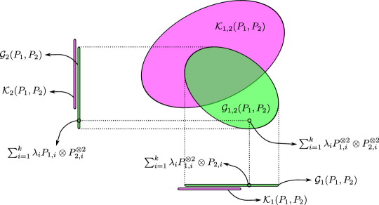
(a) By the assumption ${\mathcal{G}}\left(P_{1},P_{2}\right)\neq\emptyset$, there exists a distribution $\sum_{i=1}^{k}\lambda_{i}P_{1,i}^{\otimes 2}\otimes P_{2,i}^{\otimes 2}\notin{\mathcal{K}}_{{1,2}}\left(P_{1},P_{2}\right)$ such that $\sum_{i=1}^{k}\lambda_{i}P_{1,i}^{\otimes 2}\otimes P_{2,i}\notin{\mathcal{K}}_{{1}}\left(P_{1},P_{2}\right)$ and $\sum_{i=1}^{k}\lambda_{i}P_{1,i}\otimes P_{2,i}^{\otimes 2}\notin{\mathcal{K}}_{{2}}\left(P_{1},P_{2}\right)$ (see Equation 70).

(b) A pictorial explanation of our code construction from $\sum_{i=1}^{k}\lambda_{i}P_{1,i}^{\otimes 2}\otimes P_{2,i}^{\otimes 2}$. The construction can be viewed as an application of coded time-sharing where the time-sharing sequence is given by the convex combination coefficients $\left\{\lambda_{i}\right\}_{i=1}^{k}$. For any fixed value $\ell\in[k]$ of the time-sharing variable, each symbol of ${\mathcal{C}}_{i}$ is i.i.d. according to $P_{\ell,i}$.

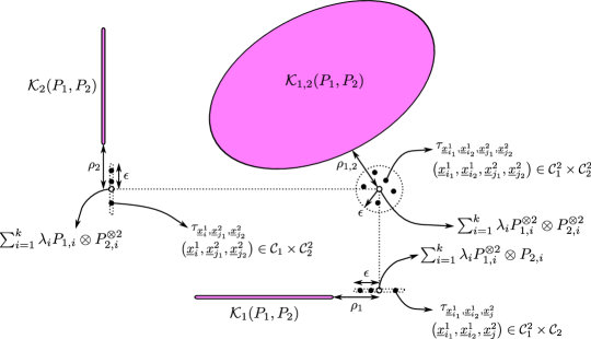
(c) By the assumption that $\sum_{i=1}^{k}\lambda_{i}P_{1,i}^{\otimes 2}\otimes P_{2,i}^{\otimes 2}$ is $\rho_{1,2}$-far from ${\mathcal{K}}_{{1,2}}\left(P_{1},P_{2}\right)$, $\sum_{i=1}^{k}\lambda_{i}P_{1,i}^{\otimes 2}\otimes P_{2,i}$ is $\rho_{1}$-far from ${\mathcal{K}}_{{1}}\left(P_{1},P_{2}\right)$ and $\sum_{i=1}^{k}\lambda_{i}P_{1,i}\otimes P_{2,i}^{\otimes 2}$ is $\rho_{2}$-far from ${\mathcal{K}}_{{2}}\left(P_{1},P_{2}\right)$, one can show via a Chernoff-union-type argument that all joint types of $({\mathcal{C}}_{1},{\mathcal{C}}_{2})$ are $\varepsilon$-far from the confusability sets and hence $({\mathcal{C}}_{1},{\mathcal{C}}_{2})$ attains positive rates and zero error. The gap factors $\rho_{1,2},\rho_{1},\rho_{2}$ and $\varepsilon$ are defined in Equation 72.

Figure 3: Illustration of the proof of Item 1 of Lemma 23. Under the assumption ${\mathcal{G}}\left(P_{1},P_{2}\right)\neq\emptyset$, the goal is to show the existence of zero-error code pairs $({\mathcal{C}}_{1},{\mathcal{C}}_{2})$ of positive rates.

We can apply similar Chernoff-union argument to the $\ell$-th punctured codes of $({\mathcal{C}}_{1},{\mathcal{C}}_{2})$ for each $\ell\in[k]$ and then take a union bound over ${\ell}$. Here by the $\ell$-th punctured codes we mean the codes obtained by restricting codewords to ${\mathcal{I}}_{\ell}$. We use ${\underline{\mathbf{x}}}_{i,{\ell}}^{1}\in{\mathcal{X}}_{1}^{\lambda_{\ell}n}$ and ${\underline{\mathbf{x}}}_{j,{\ell}}^{2}\in{\mathcal{X}}_{2}^{\lambda_{\ell}n}$ to denote respectively the subsequences of ${\underline{\mathbf{x}}}^{1}_{i}$ and ${\underline{\mathbf{x}}}^{2}_{j}$ whose components are in ${\mathcal{I}}_{\ell}$. Note that for any $1\leq i_{1}<i_{2}\leq M_{1}$ and $1\leq j_{1}<j_{2}\leq M_{2}$, by 4,

$$\mathbb{E}\left[\tau_{{\underline{\mathbf{x}}}^{1}_{i_{1}},{\underline{\mathbf{x}}}^{1}_{i_{2}},{\underline{\mathbf{x}}}^{2}_{j_{1}},{\underline{\mathbf{x}}}^{2}_{j_{2}}}\right]= \sum_{\ell=1}^{k}\lambda_{\ell}\mathbb{E}\left[\tau_{{\underline{\mathbf{x}}}^{1}_{i_{1},\ell},{\underline{\mathbf{x}}}^{1}_{i_{2},\ell},{\underline{\mathbf{x}}}^{2}_{j_{1},\ell},{\underline{\mathbf{x}}}^{2}_{j_{2},\ell}}\right]=\sum_{\ell=1}^{k}\lambda_{\ell}P_{1,\ell}^{\otimes 2}\otimes P_{2,\ell}^{\otimes 2}=P_{{\mathbf{x}}^{1}_{1},{\mathbf{x}}^{1}_{2},{\mathbf{x}}^{2}_{1},{\mathbf{x}}^{2}_{2}},$$

$$\mathbb{E}\left[\tau_{{\underline{\mathbf{x}}}^{1}_{i_{1}},{\underline{\mathbf{x}}}^{1}_{i_{2}},{\underline{\mathbf{x}}}^{2}_{j_{1}}}\right]= \sum_{\ell=1}^{k}\lambda_{\ell}\mathbb{E}\left[\tau_{{\underline{\mathbf{x}}}^{1}_{i_{1},\ell},{\underline{\mathbf{x}}}^{1}_{i_{2},\ell},{\underline{\mathbf{x}}}^{2}_{j_{1},\ell}}\right]=\sum_{\ell=1}^{k}\lambda_{\ell}P_{1,\ell}^{\otimes 2}\otimes P_{2,\ell}=P_{{\mathbf{x}}^{1}_{1},{\mathbf{x}}^{1}_{2},{\mathbf{x}}^{2}},$$

$$\mathbb{E}\left[\tau_{{\underline{\mathbf{x}}}^{1}_{i_{1}},{\underline{\mathbf{x}}}^{2}_{j_{1}},{\underline{\mathbf{x}}}^{2}_{j_{2}}}\right]= \sum_{\ell=1}^{k}\lambda_{\ell}\mathbb{E}\left[\tau_{{\underline{\mathbf{x}}}^{1}_{i_{1},\ell},{\underline{\mathbf{x}}}^{2}_{j_{1},\ell},{\underline{\mathbf{x}}}^{2}_{j_{2},\ell}}\right]=\sum_{\ell=1}^{k}\lambda_{\ell}P_{1,\ell}\otimes P_{2,\ell}^{\otimes 2}=P_{{\mathbf{x}}^{1},{\mathbf{x}}^{2}_{1},{\mathbf{x}}^{2}_{2}}.$$

Let ${\mathcal{C}}_{i}^{\prime}$ be the subcode of ${\mathcal{C}}_{i}$ such that all codewords in ${\mathcal{C}}_{i}^{\prime}$ restricted to ${\mathcal{I}}_{\ell}$ are $P_{i,\ell}$-constant composition ($i=1,2,\ell\in[k]$). The size of ${\mathcal{C}}_{i}^{\prime}$ can be concentrated similarly as before.

$$\mathbb{E}\left[|{\mathcal{C}}_{i}^{\prime}|\right]= \sum_{j=1}^{M_{i}}\Pr\left[\forall\ell\in[k],\;\tau_{{\underline{\mathbf{x}}}^{i}_{j,\ell}}=P_{i,\ell}\right]=\sum_{j=1}^{M_{i}}\prod_{\ell=1}^{k}\Pr\left[\tau_{{\underline{\mathbf{x}}}^{i}_{j,\ell}}=P_{i,\ell}\right]\asymp M_{i}\prod_{\ell=1}^{k}\nu(P_{i,\ell},\lambda_{\ell}n)^{-1}.$$

By Lemma 2,

$$\Pr\left[|{\mathcal{C}}_{i}^{\prime}|\notin(1\pm 1/2)\mathbb{E}\left[|{\mathcal{C}}_{i}^{\prime}|\right]\right]\leq 2\exp\left(-\frac{M_{i}}{12\prod_{\ell=1}^{k}\nu(P_{i,\ell},\lambda_{\ell}n)}\right).$$ (71)

Let

$$\rho_{1,2}\coloneqq d_{{\infty}}\left(P_{{\mathbf{x}}^{1}_{1},{\mathbf{x}}^{1}_{2},{\mathbf{x}}^{2}_{1},{\mathbf{x}}^{2}_{2}},{\mathcal{K}}_{{1,2}}\left(P_{1},P_{2}\right)\right)>0,$$ (72)

$$\rho_{1}\coloneqq d_{{\infty}}\left(P_{{\mathbf{x}}^{1}_{1},{\mathbf{x}}^{1}_{2},{\mathbf{x}}^{2}},{\mathcal{K}}_{{1}}\left(P_{1},P_{2}\right)\right)>0,$$

$$\rho_{2}\coloneqq d_{{\infty}}\left(P_{{\mathbf{x}}^{1},{\mathbf{x}}^{2}_{1},{\mathbf{x}}^{2}_{2}},{\mathcal{K}}_{{2}}\left(P_{1},P_{2}\right)\right)>0,$$

$$\varepsilon\coloneqq \frac{1}{2}\min\left\{\rho_{1,2},\rho_{1},\rho_{2}\right\}>0.$$

For any $1\leq i_{1}<i_{2}\leq M_{1}$ and $1\leq j_{1}<j_{2}\leq M_{2}$,

$$\Pr\left[\tau_{{\underline{\mathbf{x}}}^{1}_{i_{1}},{\underline{\mathbf{x}}}^{1}_{i_{2}},{\underline{\mathbf{x}}}^{2}_{j_{1}},{\underline{\mathbf{x}}}^{2}_{j_{2}}}\in{\mathcal{K}}_{{1,2}}\left(P_{1},P_{2}\right)\right]\leq \Pr\left[\exists\ell\in[k],\;d_{{\infty}}\left(\tau_{{\underline{\mathbf{x}}}^{1}_{i_{1},\ell},{\underline{\mathbf{x}}}^{1}_{i_{2},\ell},{\underline{\mathbf{x}}}^{2}_{j_{1},\ell},{\underline{\mathbf{x}}}^{2}_{j_{2},\ell}},P_{1,\ell}^{\otimes 2}\otimes P_{2,\ell}^{\otimes 2}\right)\geq\varepsilon\right]$$ (73)

$$\leq k\cdot\left|{\mathcal{X}}_{1}\right|^{2}\left|{\mathcal{X}}_{2}\right|^{2}\cdot 2\exp\left(-\frac{n\varepsilon^{2}}{3}\right).$$ (74)

Equation 73 follows since $d_{{\infty}}\left(\tau_{{\underline{\mathbf{x}}}^{1}_{i_{1},\ell},{\underline{\mathbf{x}}}^{1}_{i_{2},\ell},{\underline{\mathbf{x}}}^{2}_{j_{1},\ell},{\underline{\mathbf{x}}}^{2}_{j_{2},\ell}},P_{1,\ell}^{\otimes 2}\otimes P_{2,\ell}^{\otimes 2}\right)<\varepsilon$ for all $\ell\in[k]$ implies

$$d_{{\infty}}\left(\tau_{{\underline{\mathbf{x}}}^{1}_{i_{1}},{\underline{\mathbf{x}}}^{1}_{i_{2}},{\underline{\mathbf{x}}}^{2}_{j_{1}},{\underline{\mathbf{x}}}^{2}_{j_{2}}},P_{{\mathbf{x}}^{1}_{1},{\mathbf{x}}^{1}_{2},{\mathbf{x}}^{2}_{1},{\mathbf{x}}^{2}_{2}}\right)$$

$$= \max_{(x^{1}_{1},x^{1}_{2},x^{2}_{1},x^{2}_{2})\in{\mathcal{X}}_{1}^{2}\times{\mathcal{X}}_{2}^{2}}\left|\sum_{\ell=1}^{k}\lambda_{\ell}\tau_{{\underline{\mathbf{x}}}^{1}_{i_{1},\ell},{\underline{\mathbf{x}}}^{1}_{i_{2},\ell},{\underline{\mathbf{x}}}^{2}_{j_{1},\ell},{\underline{\mathbf{x}}}^{2}_{j_{2},\ell}}(x^{1}_{1},x^{1}_{2},x^{2}_{1},x^{2}_{2})-\sum_{\ell=1}^{k}\lambda_{\ell}P_{1,\ell}^{\otimes 2}\otimes P_{2,\ell}^{\otimes 2}(x^{1}_{1},x^{1}_{2},x^{2}_{1},x^{2}_{2})\right|$$

$$\leq \sum_{\ell=1}^{k}\lambda_{\ell}\max_{(x^{1}_{1},x^{1}_{2},x^{2}_{1},x^{2}_{2})\in{\mathcal{X}}_{1}^{2}\times{\mathcal{X}}_{2}^{2}}\left|\tau_{{\underline{\mathbf{x}}}^{1}_{i_{1},\ell},{\underline{\mathbf{x}}}^{1}_{i_{2},\ell},{\underline{\mathbf{x}}}^{2}_{j_{1},\ell},{\underline{\mathbf{x}}}^{2}_{j_{2},\ell}}(x^{1}_{1},x^{1}_{2},x^{2}_{1},x^{2}_{2})-P_{1,\ell}^{\otimes 2}\otimes P_{2,\ell}^{\otimes 2}(x^{1}_{1},x^{1}_{2},x^{2}_{1},x^{2}_{2})\right|$$

$$= \sum_{\ell=1}^{k}\lambda_{\ell}d_{{\infty}}\left(\tau_{{\underline{\mathbf{x}}}^{1}_{i_{1},\ell},{\underline{\mathbf{x}}}^{1}_{i_{2},\ell},{\underline{\mathbf{x}}}^{2}_{j_{1},\ell},{\underline{\mathbf{x}}}^{2}_{j_{2},\ell}},P_{1,\ell}^{\otimes 2}\otimes P_{2,\ell}^{\otimes 2}\right)<\varepsilon<\rho_{1,2},$$

which in turn implies $\tau_{{\underline{\mathbf{x}}}^{1}_{i_{1}},{\underline{\mathbf{x}}}^{1}_{i_{2}},{\underline{\mathbf{x}}}^{2}_{j_{1}},{\underline{\mathbf{x}}}^{2}_{j_{2}}}\notin{\mathcal{K}}_{{1,2}}\left(P_{1},P_{2}\right)$. In Equation 74, we took a union bound over $\ell\in[k]$ where $k={\mathcal{O}}(1)$.

Similarly, we have

$$\Pr\left[\tau_{{\underline{\mathbf{x}}}^{1}_{i_{1}},{\underline{\mathbf{x}}}^{1}_{i_{2}},{\underline{\mathbf{x}}}^{2}_{j}}\in{\mathcal{K}}_{{1}}\left(P_{1},P_{2}\right)\right]\leq k\cdot\left|{\mathcal{X}}_{1}\right|^{2}\left|{\mathcal{X}}_{2}\right|\cdot 2\exp\left(-\frac{n\varepsilon^{2}}{3}\right),$$ (75)

for all $1\leq i_{1}<i_{2}\leq M_{1}$ and $1\leq j\leq M_{2}$; and

$$\Pr\left[\tau_{{\underline{\mathbf{x}}}^{1}_{i},{\underline{\mathbf{x}}}^{2}_{j_{1}},{\underline{\mathbf{x}}}^{2}_{j_{2}}}\in{\mathcal{K}}_{{2}}\left(P_{1},P_{2}\right)\right]\leq k\cdot\left|{\mathcal{X}}_{1}\right|\left|{\mathcal{X}}_{2}\right|^{2}\cdot 2\exp\left(-\frac{n\varepsilon^{2}}{3}\right),$$ (76)

for all $1\leq i\leq M_{1}$ and $1\leq j_{1}<j_{2}\leq M_{2}$. Taking further union bounds on Equations 74, 75 and 76 over $((i_{1},i_{2}),(j_{1},j_{2}))$, $((i_{1},i_{2}),j)$ and $(i,(j_{1},j_{2}))$ respectively ensures that Equations 66, 67 and 68 still hold. The rest of the proof remains the same and we get a good code pair $({\mathcal{C}}_{1}^{\prime},{\mathcal{C}}_{2}^{\prime})$ of rate $R({\mathcal{C}}_{1}^{\prime})>0,R({\mathcal{C}}_{2}^{\prime})>0$. ∎

Proof of Items 2 and 3.

We only prove Item 2 since Item 3 is the same once the roles of the first and second users are swapped.

Suppose $P_{{\mathbf{x}}^{1}_{1},{\mathbf{x}}^{1}_{2},{\mathbf{x}}^{2}}\in{\mathcal{G}}_{{1}}\left(P_{1},P_{2}\right)\setminus{\mathcal{K}}_{{1}}\left(P_{1},P_{2}\right)$ has a decomposition $P_{{\mathbf{x}}^{1}_{1},{\mathbf{x}}^{1}_{2},{\mathbf{x}}^{2}}=\sum_{\ell=1}^{k}\lambda_{\ell}P_{1,\ell}^{\otimes 2}\otimes P_{2,\ell}$ for some $k\in{\mathbb{Z}}_{\geq 1}$, $\left\{\lambda_{\ell}\right\}_{\ell=1}^{k}\subset(0,1]$ with $\sum_{\ell=1}^{k}\lambda_{\ell}=1$ and $\left\{P_{1,\ell}\right\}_{\ell=1}^{k}\subset\Delta({\mathcal{X}}_{1}^{2})$, $\left\{P_{2,\ell}\right\}_{\ell=1}^{k}\subset\Delta({\mathcal{X}}_{2}^{2})$.

Partition $[n]$ into $k$ subsets ${\mathcal{I}}_{1},\cdots,{\mathcal{I}}_{k}$ such that $|{\mathcal{I}}_{\ell}|=\lambda_{\ell}n$ (${\ell}\in[k]$). Construct a codebook pair $({\mathcal{C}}_{1},{\mathcal{C}}_{2})$ as follows. The second codebook ${\mathcal{C}}_{2}$ only consists of one (arbitrary) codeword ${\underline{x}}^{2}\in{\mathcal{X}}_{2}^{n}$ satisfying the following property. Let ${\underline{x}}^{2}_{\ell}\in{\mathcal{X}}_{2}^{\lambda_{\ell}n}$ denote the subsequence of ${\underline{x}}^{2}$ restricted to ${\mathcal{I}}_{\ell}$. For each $\ell\in[k]$, $\tau_{{\underline{x}}^{2}_{\ell}}=P_{2,\ell}$. The first codebook ${\mathcal{C}}_{1}\in{\mathcal{X}}_{1}^{M\times n}$ consists of $M$ codewords ${\underline{\mathbf{x}}}^{1}_{1},\cdots,{\underline{\mathbf{x}}}^{1}_{M}$, where for each $i\in[M]$ and $\ell\in[k]$, ${\underline{\mathbf{x}}}^{1}_{i,\ell}\overset{\mathrm{i.i.d.}}{\sim}P_{1,\ell}^{\otimes(\lambda_{\ell}n)}$. Note that for all $1\leq i_{1}<i_{2}\leq M$, $\mathbb{E}\left[\tau_{{\underline{\mathbf{x}}}^{1}_{i_{1}},{\underline{\mathbf{x}}}^{1}_{i_{2}},{\underline{x}}^{2}}\right]=P_{{\mathbf{x}}^{1}_{1},{\mathbf{x}}^{1}_{2},{\mathbf{x}}^{2}}$. Let ${\mathcal{C}}_{1}^{\prime}$ be the subcode of ${\mathcal{C}}_{1}$ whose codewords restricted to ${\mathcal{I}}_{\ell}$ are all $P_{1,\ell}$-constant composition ($\ell\in[k]$). For ${\mathcal{C}}_{1}^{\prime}$, Equation 71 still holds. Therefore, $R({\mathcal{C}}_{1}^{\prime})\asymp R({\mathcal{C}}_{1})$ ($n\to\infty$). We define $\rho_{1}$ in the same way as in Equation 72. Let $\varepsilon\coloneqq\rho_{1}/2$. Since

$$d_{{\infty}}\left(\tau_{{\underline{\mathbf{x}}}^{1}_{i_{1}},{\underline{\mathbf{x}}}^{1}_{i_{2}},{\underline{x}}^{2}},P_{{\mathbf{x}}^{1}_{1},{\mathbf{x}}^{1}_{2},{\mathbf{x}}^{2}}\right)\leq \sum_{\ell=1}^{k}\lambda_{\ell}d_{{\infty}}\left(\tau_{{\underline{\mathbf{x}}}^{1}_{i_{1},\ell},{\underline{\mathbf{x}}}^{1}_{i_{2},\ell},{\underline{x}}^{2}_{\ell}},P_{1,\ell}^{\otimes 2}\otimes P_{2,\ell}\right),$$

a Chernoff-union bound gives

$$\Pr\left[\tau_{{\underline{\mathbf{x}}}^{1}_{i_{1}},{\underline{\mathbf{x}}}^{1}_{i_{2}},{\underline{x}}^{2}}\in{\mathcal{K}}_{{1}}\left(P_{1},P_{2}\right)\right]\leq \Pr\left[d_{{\infty}}\left(\tau_{{\underline{\mathbf{x}}}^{1}_{i_{1}},{\underline{\mathbf{x}}}^{1}_{i_{2}},{\underline{x}}^{2}},P_{{\mathbf{x}}^{1}_{1},{\mathbf{x}}^{1}_{2},{\mathbf{x}}^{2}}\right)\geq\varepsilon\right]$$

$$\leq \Pr\left[\exists\ell\in[k],\;d_{{\infty}}\left(\tau_{{\underline{\mathbf{x}}}^{1}_{i_{1},\ell},{\underline{\mathbf{x}}}^{1}_{i_{2},\ell},{\underline{x}}^{2}_{\ell}},P_{1,\ell}^{\otimes 2}\otimes P_{2,\ell}\right)\geq\varepsilon\right]$$

$$\leq k\cdot\left|{\mathcal{X}}_{1}\right|^{2}\cdot 2\exp\left(-\frac{n\varepsilon^{2}}{3}\right).$$

Since $k$ is a constant independent of $n$, a union bound over $(i_{1},i_{2})\in\binom{[|{\mathcal{C}}_{1}^{\prime}|]}{2}$ gives Equation 69. Under a proper choice of $R_{1}>0$, we get that $({\mathcal{C}}_{1}^{\prime},{\mathcal{C}}_{2})$ is a good codebook pair with probability at least $1-2^{-\Omega(n)}$. ∎

Remark 14.

In the above proof of Lemma 23, the partition $\left\{{\mathcal{I}}_{\ell}\right\}_{\ell=1}^{k}$ can be thought of as a time-sharing sequence ${\underline{u}}\in[k]^{n}$ of type $P_{\mathbf{u}}$ given by the coefficients $\left\{\lambda_{i}\right\}_{i=1}^{k}$ of the convex combination. That is, $P_{\mathbf{u}}(u)=\lambda_{u}$ for any $u\in[k]$. This particular type of time-sharing scheme is known as the coded time-sharing in the literature [PS19]. As explained in [PS19, Remark 6], the classical operational time-sharing in network information theory does not work for (oblivious) arbitrarily varying channels with constraints. This is because the adversary can concentrate his power on coordinates in a single ${\mathcal{I}}_{\ell}$. This effectively increases the noise level in ${\mathcal{I}}_{\ell}$ significantly and the $\ell$-th component codebook in the time-sharing is not necessarily resilient to this effective level of noise. The above argument also applies to the omniscient adversarial channel model. More discussions on the “non-tensorization” of good codes for adversarial channels and its implications to single-letterization of capacity expressions can be found in Item 5 of Section XVI. These phenomena suggest that the capacity region of adversarial channels does not have to be convex in general (see Section XI-A).

Furthermore, we emphasize the following point in the above achievability proof. Each component $P_{1,\ell}$ and $P_{2,\ell}$ of the convex combinations is not necessarily non-confusable, i.e., $P_{1,\ell}^{\otimes 2}\otimes P_{2,\ell}^{\otimes 2}$, $P_{1,\ell}^{\otimes 2}\otimes P_{2,\ell}$ or $P_{1,\ell}\otimes P_{2,\ell}^{\otimes 2}$ may be confusable. Nonetheless, it is only desired that their convex combinations are non-confusable.

Remark 15.

In the above proof of Items 2 and 3, the transmitter with zero capacity cannot even reliably transmit a single bit through the MAC since the codebook contains only one codeword. Such achievability proofs go through as long as there exist non-marginally confusable distributions. In contrast, in the AVMAC setting [PS19], besides non-marginal symmetrizability, non-joint symmetrizability is a necessary condition for achieving any positive rate even individually instead of jointly. More discussions on the differences between our results and Pereg–Steinberg’s [PS19] can be found in Section XI-B.

XIII-C Inner bounds via product distributions

Lemma 24 (Inner bounds via product distributions).

Fix input distributions $(P_{1},P_{2})\in\Gamma_{1}\times\Gamma_{2}$.

1. If $P_{1}^{\otimes 2}\otimes P_{2}^{\otimes 2}\notin{\mathcal{K}}_{{1,2}}\left(P_{1},P_{2}\right)$, $P_{1}\notin{\mathcal{K}}_{{1}}\left(P_{1},P_{2}\right)$ and $P_{2}\notin{\mathcal{K}}_{{2}}\left(P_{1},P_{2}\right)$, then rate pairs $(R_{1},R_{2})\in{\mathbb{R}}_{\geq 0}^{2}$ satisfying

   $$R_{1}\leq D(P_{1},P_{2})-\widehat{D}(P_{1},P_{2})$$ (77)

   $$R_{2}\leq D(P_{1},P_{2})-\widehat{D}(P_{1},P_{2})$$

   $$R_{1}+R_{2}\leq \widehat{D}(P_{1},P_{2})$$

   are achievable, where

   $$D(P_{1},P_{2})\coloneqq \min_{P_{{\mathbf{x}}^{1}_{1},{\mathbf{x}}^{1}_{2},{\mathbf{x}}^{2}_{1},{\mathbf{x}}^{2}_{2}}\in{\mathcal{K}}_{{1,2}}\left(P_{1},P_{2}\right)}D\left(P_{{\mathbf{x}}^{1}_{1},{\mathbf{x}}^{1}_{2},{\mathbf{x}}^{2}_{1},{\mathbf{x}}^{2}_{2}}\middle\|P_{1}^{\otimes 2}\otimes P_{2}^{\otimes 2}\right)$$

   $$\widehat{D}(P_{1},P_{2})\coloneqq \min\left\{\min_{P_{{\mathbf{x}}^{1}_{1},{\mathbf{x}}^{1}_{2},{\mathbf{x}}^{2}}\in{\mathcal{K}}_{{1}}\left(P_{1},P_{2}\right)}D\left(P_{{\mathbf{x}}^{1}_{1},{\mathbf{x}}^{1}_{2},{\mathbf{x}}^{2}}\middle\|P_{1}^{\otimes 2}\otimes P_{2}\right),\min_{P_{{\mathbf{x}}^{1},{\mathbf{x}}^{2}_{1},{\mathbf{x}}^{2}_{2}}\in{\mathcal{K}}_{{2}}\left(P_{1},P_{2}\right)}D\left(P_{{\mathbf{x}}^{1},{\mathbf{x}}^{2}_{1},{\mathbf{x}}^{2}_{2}}\middle\|P_{1}\otimes P_{2}^{\otimes 2}\right)\right\}.$$

2. If $P_{1}^{\otimes 2}\otimes P_{2}^{\otimes 2}\notin{\mathcal{K}}_{{1,2}}\left(P_{1},P_{2}\right)$, $P_{1}^{\otimes 2}\notin{\mathcal{K}}_{{1}}\left(P_{1},P_{2}\right)$ and $P_{2}^{\otimes 2}\in{\mathcal{K}}_{{2}}\left(P_{1},P_{2}\right)$, then rate pairs $(R_{1},0)$ satisfying

   $$0\leq R_{1}\leq\min_{P_{{\mathbf{x}}^{1}_{1},{\mathbf{x}}^{1}_{2},{\mathbf{x}}^{2}}\in{\mathcal{K}}_{{1}}\left(P_{1},P_{2}\right)}D\left(P_{{\mathbf{x}}^{1}_{1},{\mathbf{x}}^{1}_{2},{\mathbf{x}}^{2}}\middle\|P_{1}^{\otimes 2}\otimes P_{2}\right)$$ (78)

   are achievable.

3. If $P_{1}^{\otimes 2}\otimes P_{2}^{\otimes 2}\notin{\mathcal{K}}_{{1,2}}\left(P_{1},P_{2}\right)$, $P_{1}^{\otimes 2}\in{\mathcal{K}}_{{1}}\left(P_{1},P_{2}\right)$ and $P_{2}^{\otimes 2}\notin{\mathcal{K}}_{{2}}\left(P_{1},P_{2}\right)$, then rate pairs $(0,R_{2})$ satisfying

   $$0\leq R_{2}\leq\min_{P_{{\mathbf{x}}^{1},{\mathbf{x}}^{2}_{1},{\mathbf{x}}^{2}_{2}}\in{\mathcal{K}}_{{2}}\left(P_{1},P_{2}\right)}D\left(P_{{\mathbf{x}}^{1},{\mathbf{x}}^{2}_{1},{\mathbf{x}}^{2}_{2}}\middle\|P_{1}\otimes P_{2}^{\otimes 2}\right)$$ (79)

   are achievable.

Corollary 25 (Inner bounds on capacity region).

Let $\mathsf{MAC}_{2}=\left({\mathcal{X}}_{1},{\mathcal{X}}_{2},{\mathcal{S}},{\mathcal{Y}},\Gamma_{1},\Gamma_{2},\Lambda,W_{{\mathbf{y}}|{\mathbf{x}},{\mathbf{s}}}\right)$ be a two-user omniscient adversarial MAC. The capacity region of $\mathsf{MAC}_{2}$ contains as a subset the following region

$$\bigcup_{\begin{subarray}{c}(P_{1},P_{2})\in\Gamma_{1}\times\Gamma_{2}\\ \text{conditions in \lx@cref{creftypecap~refnum}{itm:rate-prod-pos-pos} are satisfied}\end{subarray}}\left\{(R_{1},R_{2}):(R_{1},R_{2})\text{ satisfies }\lx@cref{creftypecap~refnum}{eqn:achieve-product-12}\right\}$$

$$\cup\bigcup_{\begin{subarray}{c}(P_{1},P_{2})\in\Gamma_{1}\times\Gamma_{2}\\ \text{conditions in \lx@cref{creftypecap~refnum}{itm:rate-prod-pos-zero} are satisfied}\end{subarray}}\left\{(R_{1},0):R_{1}\text{ satisfies \lx@cref{creftypecap~refnum}{eqn:rate-prod-pos-zero}}\right\}$$

$$\cup\bigcup_{\begin{subarray}{c}(P_{1},P_{2})\in\Gamma_{1}\times\Gamma_{2}\\ \text{conditions in \lx@cref{creftypecap~refnum}{itm:rate-prod-zero-pos} are satisfied}\end{subarray}}\left\{(0,R_{2}):R_{2}\text{ satisfies \lx@cref{creftypecap~refnum}{eqn:rate-prod-zero-pos}}\right\}.$$

Proof of Item 1.

Sample a random code pair $\left({\mathcal{C}}_{1},{\mathcal{C}}_{2}\right)\subseteq{\mathcal{X}}_{1}^{n}\times{\mathcal{X}}_{2}^{n}$ of sizes $(M_{1},M_{2})$, where ${\mathcal{C}}_{i}$ consists of codewords ${\underline{\mathbf{x}}}^{i}_{1},\cdots,{\underline{\mathbf{x}}}^{i}_{M_{i}}$ i.i.d. according to $P_{i}^{\otimes n}$ ($i=1,2$). By Lemma 1, the the expected number of codewords in ${\mathcal{C}}_{i}$ of type $P_{i}$ is asymptotically $M_{i}/\nu(P_{i},n)$. For any $1\leq i_{1}<i_{2}\leq M_{1}$ and $1\leq j_{1}<j_{2}\leq M_{2}$, by Lemma 3,

$$\Pr\left[\tau_{{\underline{\mathbf{x}}}^{1}_{i_{1}},{\underline{\mathbf{x}}}^{1}_{i_{2}},{\underline{\mathbf{x}}}^{2}_{j_{1}},{\underline{\mathbf{x}}}^{2}_{j_{2}}}\in{\mathcal{K}}_{{1,2}}\left(P_{1},P_{2}\right)\right]\doteq \sup_{P_{{\mathbf{x}}^{1}_{1},{\mathbf{x}}^{1}_{2},{\mathbf{x}}^{2}_{1},{\mathbf{x}}^{2}_{2}}\in{\mathcal{K}}_{{1,2}}\left(P_{1},P_{2}\right)}2^{-nD\left(P_{{\mathbf{x}}^{1}_{1},{\mathbf{x}}^{1}_{2},{\mathbf{x}}^{2}_{1},{\mathbf{x}}^{2}_{2}}\middle\|P_{1}^{\otimes 2}\otimes P_{2}^{\otimes 2}\right)},$$

$$\Pr\left[\tau_{{\underline{\mathbf{x}}}^{1}_{i_{1}},{\underline{\mathbf{x}}}^{1}_{i_{2}},{\underline{\mathbf{x}}}^{2}_{j_{1}}}\in{\mathcal{K}}_{{1}}\left(P_{1},P_{2}\right)\right]\doteq \sup_{P_{{\mathbf{x}}^{1}_{1},{\mathbf{x}}^{1}_{2},{\mathbf{x}}^{2}}\in{\mathcal{K}}_{{1}}\left(P_{1},P_{2}\right)}2^{-nD\left(P_{{\mathbf{x}}^{1}_{1},{\mathbf{x}}^{1}_{2},{\mathbf{x}}^{2}}\middle\|P_{1}^{\otimes 2}\otimes P_{2}\right)},$$

$$\Pr\left[\tau_{{\underline{\mathbf{x}}}^{1}_{i_{1}},{\underline{\mathbf{x}}}^{2}_{j_{1}},{\underline{\mathbf{x}}}^{2}_{j_{2}}}\in{\mathcal{K}}_{{2}}\left(P_{1},P_{2}\right)\right]\doteq \sup_{P_{{\mathbf{x}}^{1},{\mathbf{x}}^{2}_{1},{\mathbf{x}}^{2}_{2}}\in{\mathcal{K}}_{{2}}\left(P_{1},P_{2}\right)}2^{-nD\left(P_{{\mathbf{x}}^{1},{\mathbf{x}}^{2}_{1},{\mathbf{x}}^{2}_{2}}\middle\|P_{1}\otimes P_{2}^{\otimes 2}\right)}.$$

Hence the expected number of confusable tuples $({\underline{\mathbf{x}}}^{1}_{i_{1}},{\underline{\mathbf{x}}}^{1}_{i_{2}},{\underline{\mathbf{x}}}^{2}_{j_{1}},{\underline{\mathbf{x}}}^{2}_{j_{2}})$, $({\underline{\mathbf{x}}}^{1}_{i_{1}},{\underline{\mathbf{x}}}^{1}_{i_{2}},{\underline{\mathbf{x}}}^{2}_{j})$ and $({\underline{\mathbf{x}}}^{1}_{i},{\underline{\mathbf{x}}}^{2}_{j_{1}},{\underline{\mathbf{x}}}^{2}_{j_{2}})$ is respectively

$$\binom{M_{1}}{2}\binom{M_{2}}{2}2^{-n\inf D\left(P_{{\mathbf{x}}^{1}_{1},{\mathbf{x}}^{1}_{2},{\mathbf{x}}^{2}_{1},{\mathbf{x}}^{2}_{2}}\middle\|P_{1}^{\otimes 2}\otimes P_{2}^{\otimes 2}\right)}\leq M_{1}^{2}M_{2}^{2}2^{-n\inf D\left(P_{{\mathbf{x}}^{1}_{1},{\mathbf{x}}^{1}_{2},{\mathbf{x}}^{2}_{1},{\mathbf{x}}^{2}_{2}}\middle\|P_{1}^{\otimes 2}\otimes P_{2}^{\otimes 2}\right)},$$

$$\binom{M_{1}}{2}M_{2}2^{-n\inf D\left(P_{{\mathbf{x}}^{1}_{1},{\mathbf{x}}^{1}_{2},{\mathbf{x}}^{2}}\middle\|P_{1}^{\otimes 2}\otimes P_{2}\right)}\leq M_{1}^{2}M_{2}2^{-n\inf D\left(P_{{\mathbf{x}}^{1}_{1},{\mathbf{x}}^{1}_{2},{\mathbf{x}}^{2}}\middle\|P_{1}^{\otimes 2}\otimes P_{2}\right)},$$

$$M_{1}\binom{M_{2}}{2}2^{-n\inf D\left(P_{{\mathbf{x}}^{1},{\mathbf{x}}^{2}_{1},{\mathbf{x}}^{2}_{2}}\middle\|P_{1}\otimes P_{2}^{\otimes 2}\right)}\leq M_{1}M_{2}^{2}2^{-n\inf D\left(P_{{\mathbf{x}}^{1},{\mathbf{x}}^{2}_{1},{\mathbf{x}}^{2}_{2}}\middle\|P_{1}\otimes P_{2}^{\otimes 2}\right)}.$$

Pick $M_{1},M_{2}$ such that

$$M_{1}^{2}M_{2}^{2}2^{-n\inf D\left(P_{{\mathbf{x}}^{1}_{1},{\mathbf{x}}^{1}_{2},{\mathbf{x}}^{2}_{1},{\mathbf{x}}^{2}_{2}}\middle\|P_{1}^{\otimes 2}\otimes P_{2}^{\otimes 2}\right)}\leq \min\left\{\frac{M_{1}}{3\nu(P_{1},n)},\frac{M_{2}}{3\nu(P_{2},n)}\right\},$$

$$M_{1}^{2}M_{2}2^{-n\inf D\left(P_{{\mathbf{x}}^{1}_{1},{\mathbf{x}}^{1}_{2},{\mathbf{x}}^{2}}\middle\|P_{1}^{\otimes 2}\otimes P_{2}\right)}\leq \frac{M_{1}}{3\nu(P_{1},n)}$$

$$M_{1}M_{2}^{2}2^{-n\inf D\left(P_{{\mathbf{x}}^{1},{\mathbf{x}}^{2}_{1},{\mathbf{x}}^{2}_{2}}\middle\|P_{1}\otimes P_{2}^{\otimes 2}\right)}\leq \frac{M_{2}}{3\nu(P_{2},n)}.$$

This can be satisfied if

$$2R_{1}+2R_{2}-\inf D\left(P_{{\mathbf{x}}^{1}_{1},{\mathbf{x}}^{1}_{2},{\mathbf{x}}^{2}_{1},{\mathbf{x}}^{2}_{2}}\middle\|P_{1}^{\otimes 2}\otimes P_{2}^{\otimes 2}\right)\leq \min\left\{R_{1},R_{2}\right\}-o(1),$$

$$2R_{1}+R_{2}-\inf D\left(P_{{\mathbf{x}}^{1}_{1},{\mathbf{x}}^{1}_{2},{\mathbf{x}}^{2}}\middle\|P_{1}^{\otimes 2}\otimes P_{2}\right)\leq R_{1}-o(1),$$

$$R_{1}+2R_{2}-\inf D\left(P_{{\mathbf{x}}^{1},{\mathbf{x}}^{2}_{1},{\mathbf{x}}^{2}_{2}}\middle\|P_{1}\otimes P_{2}^{\otimes 2}\right)\leq R_{2}-o(1),$$

i.e.,

$$R_{1}+2R_{2}\leq \inf D\left(P_{{\mathbf{x}}^{1}_{1},{\mathbf{x}}^{1}_{2},{\mathbf{x}}^{2}_{1},{\mathbf{x}}^{2}_{2}}\middle\|P_{1}^{\otimes 2}\otimes P_{2}^{\otimes 2}\right)-o(1),$$

$$2R_{1}+R_{2}\leq \inf D\left(P_{{\mathbf{x}}^{1}_{1},{\mathbf{x}}^{1}_{2},{\mathbf{x}}^{2}_{1},{\mathbf{x}}^{2}_{2}}\middle\|P_{1}^{\otimes 2}\otimes P_{2}^{\otimes 2}\right)-o(1),$$

$$R_{1}+R_{2}\leq \min\left\{\inf D\left(P_{{\mathbf{x}}^{1}_{1},{\mathbf{x}}^{1}_{2},{\mathbf{x}}^{2}}\middle\|P_{1}^{\otimes 2}\otimes P_{2}\right)-o(1),\inf D\left(P_{{\mathbf{x}}^{1},{\mathbf{x}}^{2}_{1},{\mathbf{x}}^{2}_{2}}\middle\|P_{1}\otimes P_{2}^{\otimes 2}\right)-o(1)\right\}.$$

That is, it suffices to take $(R_{1},R_{2})$ satisfying Equation 77 (as $n\to\infty$).

Now, we remove all codewords from ${\mathcal{C}}_{1}$ and ${\mathcal{C}}_{2}$ whose types are not $P_{1}$ and $P_{2}$ respectively. For all $1\leq i_{1}<i_{2}\leq M_{1}$ and $1\leq j_{1}<j_{2}\leq M_{2}$, we also remove

1. one of $({\underline{\mathbf{x}}}^{1}_{i_{1}},{\underline{\mathbf{x}}}^{1}_{j_{2}})$ from ${\mathcal{C}}_{1}$ and one of $({\underline{\mathbf{x}}}^{2}_{j_{1}},{\underline{\mathbf{x}}}^{2}_{j_{2}})$ from ${\mathcal{C}}_{2}$ if $\tau_{{\underline{\mathbf{x}}}^{1}_{i_{1}},{\underline{\mathbf{x}}}^{1}_{i_{2}},{\underline{\mathbf{x}}}^{2}_{j_{1}},{\underline{\mathbf{x}}}^{2}_{j_{2}}}\in{\mathcal{K}}_{{1,2}}\left(P_{1},P_{2}\right)$;

2. one of $({\underline{\mathbf{x}}}^{1}_{i_{1}},{\underline{\mathbf{x}}}^{1}_{i_{2}})$ from ${\mathcal{C}}_{1}$ if $\tau_{{\underline{\mathbf{x}}}^{1}_{i_{1}},{\underline{\mathbf{x}}}^{1}_{i_{2}},{\underline{\mathbf{x}}}^{2}_{j_{1}}}\in{\mathcal{K}}_{{1}}\left(P_{1},P_{2}\right)$;

3. one of $({\underline{\mathbf{x}}}^{2}_{j_{1}},{\underline{\mathbf{x}}}^{2}_{j_{2}})$ from ${\mathcal{C}}_{2}$ if $\tau_{{\underline{\mathbf{x}}}^{1}_{i_{1}},{\underline{\mathbf{x}}}^{2}_{j_{1}},{\underline{\mathbf{x}}}^{2}_{j_{2}}}\in{\mathcal{K}}_{{2}}\left(P_{1},P_{2}\right)$.

After the removal, $\left({\mathcal{C}}_{1},{\mathcal{C}}_{2}\right)$ becomes a good code pair. In total, the expected number of codewords we removed from ${\mathcal{C}}_{i}$ is at most

$$M_{i}-\frac{M_{i}}{\nu(P_{i},n)}+\frac{M_{i}}{3\nu(P_{i},n)}+\frac{M_{i}}{3\nu(P_{i},n)}=M_{i}-\frac{M_{i}}{3\nu(P_{i},n)}$$

for $i=1,2$. Therefore, $(R_{1},R_{2})$ is preserved after the removal. Noting that we have exhibited the existence of code pairs that attain zero error for $\mathsf{MAC}_{2}$ with desired rates, we finish the proof. ∎

Proof of Items 2 and 3.

We only prove Item 2. Item 3 will follow verbatim. Let ${\underline{x}}^{2}\in{\mathcal{X}}_{2}^{n}$ be an arbitrary codeword of type $P_{2}$. The codebook ${\mathcal{C}}_{2}$ only consists of ${\underline{x}}^{2}$. The codebook ${\mathcal{C}}_{1}$ consists of $M$ codewords ${\underline{\mathbf{x}}}^{1}_{1},\cdots,{\underline{\mathbf{x}}}^{1}_{M}$ i.i.d. according to $P_{1}^{\otimes n}$. Again, the expected number of codewords in ${\mathcal{C}}_{1}$ of type $P_{1}$ is asymptotically $M/\nu(P_{1},n)$. By Lemma 3, for any $1\leq i_{1}<i_{2}\leq M$,

$$\Pr\left[\tau_{{\underline{\mathbf{x}}}^{1}_{i_{1}},{\underline{\mathbf{x}}}^{1}_{i_{2}},{\underline{x}}^{2}}\in{\mathcal{K}}_{{1}}\left(P_{1},P_{2}\right)\right]\doteq \sup_{P_{{\mathbf{x}}^{1}_{1},{\mathbf{x}}^{1}_{2},{\mathbf{x}}^{2}}\in{\mathcal{K}}_{{1}}\left(P_{1},P_{2}\right)}2^{-nD\left(P_{{\mathbf{x}}^{1}_{1},{\mathbf{x}}^{1}_{2},{\mathbf{x}}^{2}}\middle\|P_{1}^{\otimes 2}\otimes P_{2}\right)}.$$

Hence the expected number of confusable tuples $({\underline{\mathbf{x}}}^{1}_{i_{1}},{\underline{\mathbf{x}}}^{1}_{i_{2}},{\underline{x}}^{2})$ is

$$\binom{M}{2}2^{-n\inf D\left(P_{{\mathbf{x}}^{1}_{1},{\mathbf{x}}^{1}_{2},{\mathbf{x}}^{2}}\middle\|P_{1}^{\otimes 2}\otimes P_{2}\right)}\leq M^{2}2^{-n\inf D\left(P_{{\mathbf{x}}^{1}_{1},{\mathbf{x}}^{1}_{2},{\mathbf{x}}^{2}}\middle\|P_{1}^{\otimes 2}\otimes P_{2}\right)}.$$

Pick $M$ such that

$$M^{2}2^{-n\inf D\left(P_{{\mathbf{x}}^{1}_{1},{\mathbf{x}}^{1}_{2},{\mathbf{x}}^{2}}\middle\|P_{1}^{\otimes 2}\otimes P_{2}\right)}\leq \frac{M}{2\nu(P_{1},n)}.$$

It suffices to take

$$2R_{1}-\inf D\left(P_{{\mathbf{x}}^{1}_{1},{\mathbf{x}}^{1}_{2},{\mathbf{x}}^{2}}\middle\|P_{1}^{\otimes 2}\otimes P_{2}\right)\leq R_{1}-o(1),$$

i.e., $R_{1}$ asymptotically satisfies Equation 78.

We then remove all codewords from ${\mathcal{C}}_{1}$ which have type different from $P_{1}$. We also remove ${\underline{\mathbf{x}}}^{1}_{i_{1}}$ if $\tau_{{\underline{\mathbf{x}}}^{1}_{i_{1}},{\underline{\mathbf{x}}}^{1}_{i_{2}},{\underline{x}}^{2}}\in{\mathcal{K}}_{{1}}\left(P_{1},P_{2}\right)$ for some $i_{1}<i_{2}\leq M$. After removal we get a constant composition codebook pair that attains zero error. The expected number of codewords we removed from ${\mathcal{C}}_{1}$ is at most $M-M/\nu(P_{1},n)+M/2\nu(P_{1},n)=M-M/2\nu(P_{1},n)$. Therefore, the removal does not (asymptotically) change the rate. This finishes the proof. ∎

Remark 16.

In Lemma 24, we did not obtain a pentagon region defined by three mutual information terms as is commonly seen in problems regarding MACs. It is perhaps due to our crude expurgation strategy. We believe that our inner bounds can be improved by employing more careful expurgation strategies (see Item 4 in Section XVI).

XIV Converse, Item 1 in Theorem 20

In this section, we assume that ${\mathcal{G}}\left(P_{1},P_{2}\right)=\emptyset$. Let $({\mathcal{C}}_{1},{\mathcal{C}}_{2})\subseteq{\mathcal{X}}_{1}^{n}\times{\mathcal{X}}_{2}^{n}$ be any good codebook pair. Without loss of rate, we assume that ${\mathcal{C}}_{1}$ is $P_{1}$-constant composition and ${\mathcal{C}}_{2}$ is $P_{2}$-constant composition. Our goal is to show that $R({\mathcal{C}}_{1})$ and $R({\mathcal{C}}_{2})$ cannot be simultaneously positive. In fact, we will show that at least one of $M_{1}\coloneqq|{\mathcal{C}}_{1}|$ and $M_{2}\coloneqq|{\mathcal{C}}_{2}|$ is bounded from above by a constant (independent of $n$).

XIV-A Subcode pair extraction

Definition 18 (Bipartite, uniform, complete hypergraphs).

A hypergraph ${\mathcal{H}}=({\mathcal{V}},{\mathcal{E}})$ is called $(N_{1},N_{2})$-bipartite if it is bipartite with ${\mathcal{V}}={\mathcal{V}}_{1}\sqcup{\mathcal{V}}_{2}$ where $|{\mathcal{V}}_{1}|=N_{1}$ and $|{\mathcal{V}}_{2}|=N_{2}$. It is called $(k_{1},k_{2})$-uniform if every hyperedge contains $k_{1}$ vertices in ${\mathcal{V}}_{1}$ and $k_{2}$ vertices in ${\mathcal{V}}_{2}$. It is called complete if every $k_{1}$-tuple of vertices in ${\mathcal{V}}_{1}$ and every $k_{2}$-tuple of vertices in ${\mathcal{V}}_{2}$ are connected.

Theorem 26 (Bipartite hypergraph Ramsey’s theorem [BLA76]).

Let $N_{1},N_{2},D$ be integers that are at least 2. There exist constants $K_{1}=K_{2}(N_{1},N_{2},D)$ and $K_{2}=K_{2}(N_{1},N_{2},D)$ such that for every $(M_{1},M_{2})$-bipartite $(2,2)$-uniform complete hypergraph ${\mathcal{H}}=(({\mathcal{V}}_{1},{\mathcal{V}}_{2}),{\mathcal{E}})$ such that $|{\mathcal{V}}_{1}|=M_{1}\geq K_{1}$ and $|{\mathcal{V}}_{2}|=M_{2}\geq K_{2}$, for every $D$-coloring of ${\mathcal{E}}$, there must exist ${\mathcal{V}}_{1}^{\prime}\subseteq{\mathcal{V}}_{1}$ and ${\mathcal{V}}_{2}^{\prime}\subseteq{\mathcal{V}}_{2}$ such that $|{\mathcal{V}}_{1}^{\prime}|\geq N_{1},|{\mathcal{V}}_{2}^{\prime}|\geq N_{2}$ and all hyperedges crossing ${\mathcal{V}}_{1}^{\prime}$ and ${\mathcal{V}}_{2}^{\prime}$ have the same color.

Lemma 27 (Subcode pair extraction).

For any code pair $\left({\mathcal{C}}_{1},{\mathcal{C}}_{2}\right)=\left(\left\{{\underline{x}}^{1}_{k}\right\}_{k=1}^{M_{1}},\left\{{\underline{x}}^{2}_{\ell}\right\}_{\ell=1}^{M_{2}}\right)$ of sizes $M_{1}$ and $M_{2}$, respectively, there exists a subcode pair $\left({\mathcal{C}}_{1}^{\prime},{\mathcal{C}}_{2}^{\prime}\right)=\left(\left\{{\underline{x}}^{1}_{i}\right\}_{i=1}^{M_{1}^{\prime}},\left\{{\underline{x}}^{2}_{j}\right\}_{j=1}^{M_{2}^{\prime}}\right)$ of sizes $M_{1}^{\prime}\geq f_{1}(|{\mathcal{X}}_{1}|,|{\mathcal{X}}_{2}|,\eta,M_{1},M_{2})\xrightarrow{M_{1}\to\infty}\infty$ and $M_{2}^{\prime}\geq f_{2}(|{\mathcal{X}}_{1}|,|{\mathcal{X}}_{2}|,\eta,M_{1},M_{2})\xrightarrow{M_{2}\to\infty}\infty$, respectively, and there exists a distribution $P_{{\mathbf{x}}^{1}_{1},{\mathbf{x}}^{1}_{2},{\mathbf{x}}^{2}_{1},{\mathbf{x}}^{2}_{2}}\in{\mathcal{J}}_{1,2}\left(P_{1},P_{2}\right)$ such that, for all $1\leq i_{1}<i_{2}\leq M_{1}^{\prime}$ and $1\leq j_{1}<j_{2}\leq M_{2}^{\prime}$, it holds that $d_{{\infty}}\left(\tau_{{\underline{x}}^{1}_{i_{1}},{\underline{x}}^{1}_{i_{2}},{\underline{x}}^{2}_{j_{1}},{\underline{x}}^{2}_{j_{2}}},P_{{\mathbf{x}}^{1}_{1},{\mathbf{x}}^{1}_{2},{\mathbf{x}}^{2}_{1},{\mathbf{x}}^{2}_{2}}\right)\leq\eta$.

Proof.

To apply Theorem 26, we build an $(M_{1},M_{2})$-bipartite $(2,2)$-uniform complete hypergraph ${\mathcal{H}}$. The left and right vertex sets of ${\mathcal{H}}$ are the codewords in ${\mathcal{C}}_{1}$ and the codewords in ${\mathcal{C}}_{2}$ respectively. Every pair of codewords $({\underline{x}}^{1}_{i_{1}},{\underline{x}}^{1}_{i_{2}})\in\binom{{\mathcal{C}}_{1}}{2}$ (where $1\leq i_{1}<i_{2}<M_{1}$) in the left vertex set is connected to all pairs of codewords $({\underline{x}}^{2}_{j_{1}},{\underline{x}}^{2}_{j_{2}})\in\binom{{\mathcal{C}}_{2}}{2}$ (for all $1\leq j_{1}<j_{2}\leq M_{2}$) in the right vertex set.

We now color all hyperedges of ${\mathcal{H}}$ using distributions in ${\mathcal{J}}_{1,2}\left(P_{1},P_{2}\right)$. To this end, we first take an $\eta$-net ${\mathcal{N}}$ of ${\mathcal{J}}_{1,2}\left(P_{1},P_{2}\right)$ with respect to $d_{\infty}$. By Lemma 5, $D\coloneqq\left|{\mathcal{N}}\right|$ can be made no larger than $\left(\frac{\left|{\mathcal{X}}_{1}\right|^{2}\times\left|{\mathcal{X}}_{2}\right|^{2}}{2\eta}+1\right)^{\left|{\mathcal{X}}_{1}\right|^{2}\times\left|{\mathcal{X}}_{2}\right|^{2}}$. The hyperedges in ${\mathcal{H}}$ are colored in the following way. If an hyperedge $(({\underline{x}}^{1}_{i_{1}},{\underline{x}}^{1}_{i_{2}}),({\underline{x}}^{2}_{j_{1}},{\underline{x}}^{2}_{j_{2}}))$ (where $1\leq i_{1}<i_{2}<M_{1}$ and $1\leq j_{1}<j_{2}\leq M_{2}$) satisfies $d_{{\infty}}\left(\tau_{{\underline{x}}^{1}_{i_{1}},{\underline{x}}^{1}_{i_{2}},{\underline{x}}^{2}_{j_{1}},{\underline{x}}^{2}_{j_{2}}},P_{{\mathbf{x}}^{1}_{1},{\mathbf{x}}^{1}_{2},{\mathbf{x}}^{2}_{1},{\mathbf{x}}^{2}_{2}}\right)\leq\eta$ for some $P_{{\mathbf{x}}^{1}_{1},{\mathbf{x}}^{1}_{2},{\mathbf{x}}^{2}_{1},{\mathbf{x}}^{2}_{2}}\in{\mathcal{N}}$, then we color this hyperedge by $P_{{\mathbf{x}}^{1}_{1},{\mathbf{x}}^{1}_{2},{\mathbf{x}}^{2}_{1},{\mathbf{x}}^{2}_{2}}$. Note that by the covering property of ${\mathcal{N}}$, such a distribution must exist.

By Theorem 26, there exist subcodes $({\mathcal{C}}_{1}^{\prime},{\mathcal{C}}_{2}^{\prime})$ of $({\mathcal{C}}_{1},{\mathcal{C}}_{2})$ satisfying

1. $M_{1}^{\prime}\coloneqq|{\mathcal{C}}_{1}^{\prime}|\geq N_{1},M_{2}^{\prime}\coloneqq|{\mathcal{C}}_{2}^{\prime}|\geq N_{2}$ for $N_{1}=N_{1}(M_{1},M_{2},D),N_{2}=N_{2}(M_{1},M_{2},D)$ with $N_{1}\xrightarrow{M_{1}\to\infty}\infty,N_{2}\xrightarrow{M_{2}\to\infty}\infty$;

2. all hyperedges between ${\mathcal{C}}_{1}^{\prime}$ and ${\mathcal{C}}_{2}^{\prime}$ are monochromatic.

In other words, according to the way we colored the hyperedges, there is a distribution $P_{{\mathbf{x}}^{1}_{1},{\mathbf{x}}^{1}_{2},{\mathbf{x}}^{2}_{1},{\mathbf{x}}^{2}_{2}}\in{\mathcal{J}}_{1,2}\left(P_{1},P_{2}\right)$ such that for all $1\leq i_{1}<i_{2}\leq M_{1}^{\prime}$ and $1\leq j_{1}<j_{2}\leq M_{2}^{\prime}$, we have $d_{{\infty}}\left(\tau_{{\underline{x}}^{1}_{i_{1}},{\underline{x}}^{1}_{i_{2}},{\underline{x}}^{2}_{j_{1}},{\underline{x}}^{2}_{j_{2}}},P_{{\mathbf{x}}^{1}_{1},{\mathbf{x}}^{1}_{2},{\mathbf{x}}^{2}_{1},{\mathbf{x}}^{2}_{2}}\right)\leq\eta$. This completes the proof. ∎

In what follows, we will prove that the “equicoupled” subcode pair $({\mathcal{C}}_{1}^{\prime},{\mathcal{C}}_{2}^{\prime})$ must have at least one zero rate. We do so by treating separately the case where $P_{{\mathbf{x}}^{1}_{1},{\mathbf{x}}^{1}_{2},{\mathbf{x}}^{2}_{1},{\mathbf{x}}^{2}_{2}}$ is (almost) symmetric and the case where it is (significantly) asymmetric. We will actually show that $M_{1}^{\prime}=f(M_{1})\leq C_{1}$ or $M_{2}^{\prime}=f(M_{2})\leq C_{2}$ for some constants (independent of $n$) $C_{1}>0$ and $C_{2}>0$. Since $f(\cdot)$ is a (slowly) increasing function, this implies that the original code pair $({\mathcal{C}}_{1},{\mathcal{C}}_{2})$ has sizes $M_{1}\leq f^{-1}(C_{1})$ and $M_{2}\leq f^{-1}(C_{2})$ which are still constants (though enormous). This is a stronger statement than that $({\mathcal{C}}_{1},{\mathcal{C}}_{2})$ have at least one zero rate.

XIV-B Asymmetric case

Definition 19 (Asymmetry and approximate symmetry).

The $\left\{1,2\right\}$-asymmetry, the $\left\{1\right\}$-asymmetry, the $\left\{2\right\}$-asymmetry and the asymmetry of a distribution $P_{{\mathbf{x}}^{1}_{1},{\mathbf{x}}^{1}_{2},{\mathbf{x}}^{2}_{1},{\mathbf{x}}^{2}_{2}}\in\Delta({\mathcal{X}}_{1}^{2}\times{\mathcal{X}}_{2}^{2})$ is respectively defined as

$$\mathrm{asymm}_{1,2}(P_{{\mathbf{x}}^{1}_{1},{\mathbf{x}}^{1}_{2},{\mathbf{x}}^{2}_{1},{\mathbf{x}}^{2}_{2}})\coloneqq \max_{(x^{1}_{1},x^{1}_{2})\in{{\mathcal{X}}_{1}}^{2}}\max_{(x^{2}_{1},x^{2}_{2})\in{{\mathcal{X}}_{2}}^{2}}\left|P_{{\mathbf{x}}^{1}_{1},{\mathbf{x}}^{1}_{2},{\mathbf{x}}^{2}_{1},{\mathbf{x}}^{2}_{2}}(x^{1}_{1},x^{1}_{2},x^{2}_{1},x^{2}_{2})-P_{{\mathbf{x}}^{1}_{1},{\mathbf{x}}^{1}_{2},{\mathbf{x}}^{2}_{1},{\mathbf{x}}^{2}_{2}}(x^{1}_{2},x^{1}_{1},x^{2}_{2},x^{2}_{1})\right|,$$

$$\mathrm{asymm}_{1}(P_{{\mathbf{x}}^{1}_{1},{\mathbf{x}}^{1}_{2},{\mathbf{x}}^{2}_{1},{\mathbf{x}}^{2}_{2}})\coloneqq \max_{(x^{1}_{1},x^{1}_{2})\in{{\mathcal{X}}_{1}}^{2}}\max_{(x^{2}_{1},x^{2}_{2})\in{{\mathcal{X}}_{2}}^{2}}\left|P_{{\mathbf{x}}^{1}_{1},{\mathbf{x}}^{1}_{2},{\mathbf{x}}^{2}_{1},{\mathbf{x}}^{2}_{2}}(x^{1}_{1},x^{1}_{2},x^{2}_{1},x^{2}_{2})-P_{{\mathbf{x}}^{1}_{1},{\mathbf{x}}^{1}_{2},{\mathbf{x}}^{2}_{1},{\mathbf{x}}^{2}_{2}}(x^{1}_{2},x^{1}_{1},x^{2}_{1},x^{2}_{2})\right|,$$

$$\mathrm{asymm}_{2}(P_{{\mathbf{x}}^{1}_{1},{\mathbf{x}}^{1}_{2},{\mathbf{x}}^{2}_{1},{\mathbf{x}}^{2}_{2}})\coloneqq \max_{(x^{1}_{1},x^{1}_{2})\in{{\mathcal{X}}_{1}}^{2}}\max_{(x^{2}_{1},x^{2}_{2})\in{{\mathcal{X}}_{2}}^{2}}\left|P_{{\mathbf{x}}^{1}_{1},{\mathbf{x}}^{1}_{2},{\mathbf{x}}^{2}_{1},{\mathbf{x}}^{2}_{2}}(x^{1}_{1},x^{1}_{2},x^{2}_{1},x^{2}_{2})-P_{{\mathbf{x}}^{1}_{1},{\mathbf{x}}^{1}_{2},{\mathbf{x}}^{2}_{1},{\mathbf{x}}^{2}_{2}}(x^{1}_{1},x^{1}_{2},x^{2}_{2},x^{2}_{1})\right|,$$

$$\mathrm{asymm}(P_{{\mathbf{x}}^{1}_{1},{\mathbf{x}}^{1}_{2},{\mathbf{x}}^{2}_{1},{\mathbf{x}}^{2}_{2}})\coloneqq \max\left\{\mathrm{asymm}_{1,2}(P_{{\mathbf{x}}^{1}_{1},{\mathbf{x}}^{1}_{2},{\mathbf{x}}^{2}_{1},{\mathbf{x}}^{2}_{2}}),\mathrm{asymm}_{1}(P_{{\mathbf{x}}^{1}_{1},{\mathbf{x}}^{1}_{2},{\mathbf{x}}^{2}_{1},{\mathbf{x}}^{2}_{2}}),\mathrm{asymm}_{2}(P_{{\mathbf{x}}^{1}_{1},{\mathbf{x}}^{1}_{2},{\mathbf{x}}^{2}_{1},{\mathbf{x}}^{2}_{2}})\right\}.$$

A distribution $P_{{\mathbf{x}}^{1}_{1},{\mathbf{x}}^{1}_{2},{\mathbf{x}}^{2}_{1},{\mathbf{x}}^{2}_{2}}$ is called $\alpha$-symmetric if $\mathrm{asymm}(P_{{\mathbf{x}}^{1}_{1},{\mathbf{x}}^{1}_{2},{\mathbf{x}}^{2}_{1},{\mathbf{x}}^{2}_{2}})\leq\alpha$.

Remark 17.

By definition, a self-coupling $P_{{\mathbf{x}}^{1}_{1},{\mathbf{x}}^{1}_{2},{\mathbf{x}}^{2}_{1},{\mathbf{x}}^{2}_{2}}\in{\mathcal{J}}_{1,2}\left(P_{1},P_{2}\right)$ is in ${\mathcal{S}}_{1,2}\left(P_{1},P_{2}\right)$ if and only if $\mathrm{asymm}(P_{{\mathbf{x}}^{1}_{1},{\mathbf{x}}^{1}_{2},{\mathbf{x}}^{2}_{1},{\mathbf{x}}^{2}_{2}})=0$.

According to Definition 19, the asymmetry of $P_{{\mathbf{x}}^{1}_{1},{\mathbf{x}}^{1}_{2},{\mathbf{x}}^{2}_{1},{\mathbf{x}}^{2}_{2}}$ that was extracted in Lemma 27 can be divided into eight different cases as shown in Table III below. Case (1) in Table III corresponds to the case where $P_{{\mathbf{x}}^{1}_{1},{\mathbf{x}}^{1}_{2},{\mathbf{x}}^{2}_{1},{\mathbf{x}}^{2}_{2}}$ is $\alpha$-symmetric. This case will be treated in Section XIV-C. Other cases correspond to when $P_{{\mathbf{x}}^{1}_{1},{\mathbf{x}}^{1}_{2},{\mathbf{x}}^{2}_{1},{\mathbf{x}}^{2}_{2}}$ is asymmetric with asymmetry larger than $\alpha$. They will be treated in Sections XIV-B1, XIV-B2 and XIV-B3.

Cases	$\mathrm{asymm}_{1,2}(P_{{\mathbf{x}}^{1}_{1},{\mathbf{x}}^{1}_{2},{\mathbf{x}}^{2}_{1},{\mathbf{x}}^{2}_{2}})\stackrel{{\scriptstyle?}}{{\leq}}\alpha$	$\mathrm{asymm}_{1}(P_{{\mathbf{x}}^{1}_{1},{\mathbf{x}}^{1}_{2},{\mathbf{x}}^{2}_{1},{\mathbf{x}}^{2}_{2}})\stackrel{{\scriptstyle?}}{{\leq}}\alpha$	$\mathrm{asymm}_{2}(P_{{\mathbf{x}}^{1}_{1},{\mathbf{x}}^{1}_{2},{\mathbf{x}}^{2}_{1},{\mathbf{x}}^{2}_{2}})\stackrel{{\scriptstyle?}}{{\leq}}\alpha$	Section
Case (1)	$\leq$	$\leq$	$\leq$	Section XIV-C
Case (2)	$>$	$\leq$	$\leq$	Section XIV-B3
Case (3)	$\leq$	$>$	$\leq$	Section XIV-B3
Case (4)	$\leq$	$\leq$	$>$	Section XIV-B3
Case (5)	$>$	$>$	$\leq$	Section XIV-B1
Case (6)	$>$	$\leq$	$>$	Section XIV-B1
Case (7)	$\leq$	$>$	$>$	Section XIV-B2
Case (8)	$>$	$>$	$>$	Section XIV-B2

TABLE III: The asymmetric case can be divided into several sub-cases.

For the asymmetric cases (Cases (5)-(8) in Table III), we prove the following lemma.

Lemma 28.

If a code pair $({\mathcal{C}}_{1}^{\prime},{\mathcal{C}}_{2}^{\prime})\in{\mathcal{X}}_{1}^{M_{1}^{\prime}\times n}\times{\mathcal{X}}_{2}^{M_{2}^{\prime}\times n}$ satisfies that there exists a distribution $P_{{\mathbf{x}}^{1}_{1},{\mathbf{x}}^{1}_{2},{\mathbf{x}}^{2}_{1},{\mathbf{x}}^{2}_{2}}\in{\mathcal{J}}_{1,2}\left(P_{1},P_{2}\right)$ such that

1. ${\mathcal{C}}_{i}$ is $P_{i}$-constant composition for $i=1,2$;

2. for all $1\leq i_{1}<i_{2}\leq M_{1}^{\prime}$ and $1\leq j_{1}<j_{2}\leq M_{2}^{\prime}$, $d_{{\infty}}\left(\tau_{{\underline{x}}^{1}_{i_{1}},{\underline{x}}^{1}_{i_{2}},{\underline{x}}^{2}_{j_{1}},{\underline{x}}^{2}_{j_{2}}},P_{{\mathbf{x}}^{1}_{1},{\mathbf{x}}^{1}_{2},{\mathbf{x}}^{2}_{1},{\mathbf{x}}^{2}_{2}}\right)\leq\eta$;

3. $\mathrm{asymm}(P_{{\mathbf{x}}^{1}_{1},{\mathbf{x}}^{1}_{2},{\mathbf{x}}^{2}_{1},{\mathbf{x}}^{2}_{2}})\geq\alpha$,

then at least one of $M_{1}^{\prime}$ and $M_{2}^{\prime}$ is at most a constant $C(\alpha,\eta)>0$.

Proof.

The proof is divided into several cases. As we shall see in Sections XIV-B1 and XIV-B2, only Cases (5)-(8) in Table III are asymmetric cases. Cases (2)-(4), handled in Section XIV-B3, can be reduced to the symmetric case (Case (1)). The symmetric Case (1) will be treated in the next section (Section XIV-C). ∎

The following lemma will be crucial in the proceeding subsections.

Theorem 29 ([Kom90]).

Let ${\mathbf{v}}_{1},\cdots,{\mathbf{v}}_{M}$ be a sequence of random variables over a common finite alphabet ${\mathcal{W}}$. If there exist a distribution $P_{{\mathbf{w}}_{1},{\mathbf{w}}_{2}}\in\Delta({\mathcal{W}}^{2})$ and a constant $\eta\geq 0$ such that $\left\|P_{{\mathbf{v}}_{i},{\mathbf{v}}_{j}}-P_{{\mathbf{w}}_{1},{\mathbf{w}}_{2}}\right\|_{\infty}\leq\eta$ for all $1\leq i<j\leq M$, then $\mathrm{asymm}(P_{{\mathbf{w}}_{1},{\mathbf{w}}_{2}})\leq{6}/{\sqrt{M}}+4\sqrt{\eta}+2\eta$, where

$$\mathrm{asymm}(P_{{\mathbf{w}}_{1},{\mathbf{w}}_{2}})\coloneqq \max_{(w_{1},w_{2})\in{\mathcal{W}}\times{\mathcal{W}}}\left|P_{{\mathbf{w}}_{1},{\mathbf{w}}_{2}}(w_{1},w_{2})-P_{{\mathbf{w}}_{1},{\mathbf{w}}_{2}}(w_{2},w_{1})\right|.$$

XIV-B1 Cases (5) & (6) in Table III

We only prove Case (5) since Case (6) is the same up to change of notation. We will show that $M_{1}^{\prime}\coloneqq|{\mathcal{C}}_{1}^{\prime}|$ is at most a constant.

We identify $P_{{\mathbf{x}}^{1}_{1},{\mathbf{x}}^{1}_{2},{\mathbf{x}}^{2}_{1},{\mathbf{x}}^{2}_{2}}$ with $P_{{\mathbf{x}}^{1}_{1},{\mathbf{x}}^{1}_{2},{\mathbf{z}}^{2}}$ where ${\mathbf{z}}^{2}=({\mathbf{x}}^{2}_{1},{\mathbf{x}}^{2}_{2})$ is a random variable over ${\mathcal{Z}}_{2}\coloneqq{\mathcal{X}}_{2}^{2}$. Immediately, $\alpha<\mathrm{asymm}_{1}(P_{{\mathbf{x}}^{1}_{1},{\mathbf{x}}^{1}_{2},{\mathbf{x}}^{2}_{1},{\mathbf{x}}^{2}_{2}})=\mathrm{asymm}_{1}(P_{{\mathbf{x}}^{1}_{1},{\mathbf{x}}^{1}_{2},{\mathbf{z}}^{2}})$ where $\mathrm{asymm}_{1}(P_{{\mathbf{x}}^{1}_{1},{\mathbf{x}}^{1}_{2},{\mathbf{x}}^{2}_{1},{\mathbf{x}}^{2}_{2}})$ is naturally defined as

$$\mathrm{asymm}_{1}(P_{{\mathbf{x}}^{1}_{1},{\mathbf{x}}^{1}_{2},{\mathbf{z}}^{2}})\coloneqq \max_{(x^{1}_{1},x^{1}_{2})\in{\mathcal{X}}_{1}^{2}}\max_{z^{2}\in{\mathcal{Z}}_{2}}\left|P_{{\mathbf{x}}^{1}_{1},{\mathbf{x}}^{1}_{2},{\mathbf{z}}^{2}}(x^{1}_{1},x^{1}_{2},z^{2})-P_{{\mathbf{x}}^{1}_{1},{\mathbf{x}}^{1}_{2},{\mathbf{z}}^{2}}(x^{1}_{2},x^{1}_{1},z^{2})\right|.$$

We then have the following simple lemma.

Lemma 30.

If a distribution $P_{{\mathbf{x}}^{1}_{1},{\mathbf{x}}^{1}_{2},{\mathbf{z}}^{2}}$ satisfies $\mathrm{asymm}_{1}(P_{{\mathbf{x}}^{1}_{1},{\mathbf{x}}^{1}_{2},{\mathbf{z}}^{2}})>\alpha$, then $\mathrm{asymm}(P_{{\mathbf{w}}_{1},{\mathbf{w}}_{2}})>\alpha$, where ${\mathbf{w}}_{i}\coloneqq({\mathbf{x}}^{1}_{i},{\mathbf{z}}^{2})\in{\mathcal{W}}\coloneqq{\mathcal{X}}_{1}\times{\mathcal{Z}}_{2}$ for $i=1,2$.

Proof.

The lemma follows from the following simple (in)equalities:

$$\left|P_{{\mathbf{w}}_{1},{\mathbf{w}}_{2}}(w_{1},w_{2})-P_{{\mathbf{w}}_{1},{\mathbf{w}}_{2}}(w_{2},w_{1})\right|= \left|P_{({\mathbf{x}}^{1}_{1},{\mathbf{z}}^{2}),({\mathbf{x}}^{1}_{2},{\mathbf{z}}^{2})}((x^{1}_{1},z^{2}),(x^{1}_{2},z^{2}))-P_{({\mathbf{x}}^{1}_{1},{\mathbf{z}}^{2}),({\mathbf{x}}^{1}_{2},{\mathbf{z}}^{2})}((x^{1}_{2},z^{2}),(x^{1}_{1},z^{2}))\right|$$

$$= \left|P_{{\mathbf{x}}^{1}_{1},{\mathbf{x}}^{1}_{2},{\mathbf{z}}^{2}}(x^{1}_{1},x^{1}_{2},z^{2})-P_{{\mathbf{x}}^{1}_{1},{\mathbf{x}}^{1}_{2},{\mathbf{z}}^{2}}(x^{1}_{2},x^{1}_{1},z^{2})\right|>\alpha.\qed$$ (80)

Recall $M_{1}^{\prime}\coloneqq\left|{\mathcal{C}}_{1}^{\prime}\right|,M_{2}^{\prime}\coloneqq\left|{\mathcal{C}}_{2}^{\prime}\right|$. By equicoupledness, for any fixed $1\leq j_{1}<j_{2}<M_{2}^{\prime}$, we have $d_{{\infty}}\left(\tau_{{\underline{x}}^{1}_{i_{1}},{\underline{x}}^{1}_{i_{2}},{\underline{x}}^{2}_{j_{1}},{\underline{x}}^{2}_{j_{2}}},P_{{\mathbf{x}}^{1}_{1},{\mathbf{x}}^{1}_{2},{\mathbf{x}}^{2}_{1},{\mathbf{x}}^{2}_{2}}\right)\leq\eta$ for all $1\leq i_{1}<i_{2}\leq M_{1}^{\prime}$. Identify the codewords ${\underline{x}}^{1}_{1},\cdots,{\underline{x}}^{1}_{M_{1}^{\prime}}$ in ${\mathcal{C}}_{1}^{\prime}$ together with ${\underline{x}}^{2}_{j_{1}},{\underline{x}}^{2}_{j_{2}}\in{\mathcal{C}}_{2}^{\prime}$ with a sequence of random variables ${\boldsymbol{\chi}}_{1},\cdots,{\boldsymbol{\chi}}_{M_{1}^{\prime}},{\boldsymbol{\zeta}}^{2}\in{\mathcal{X}}_{1}^{M_{1}^{\prime}}\times{\mathcal{Z}}_{2}$. That is $P_{{\boldsymbol{\chi}}_{1},\cdots,{\boldsymbol{\chi}}_{M_{1}^{\prime}},{\boldsymbol{\zeta}}^{2}}\coloneqq\tau_{{\underline{x}}^{1}_{1},\cdots,{\underline{x}}^{1}_{M_{1}^{\prime}},({\underline{x}}^{2}_{j_{1}},{\underline{x}}^{2}_{j_{2}})}$. Arrange this sequence in the following way: ${\mathbf{v}}_{1},\cdots,{\mathbf{v}}_{M_{1}^{\prime}}$ where ${\mathbf{v}}_{i}=({\boldsymbol{\chi}}_{i},{\boldsymbol{\zeta}}^{2})\in{\mathcal{W}}\coloneqq{\mathcal{X}}_{1}\times{\mathcal{Z}}_{2}$. This sequence satisfies $d_{{\infty}}\left(P_{{\mathbf{v}}_{i_{1}},{\mathbf{v}}_{i_{2}}},P_{{\mathbf{w}}_{1},{\mathbf{w}}_{2}}\right)\leq\eta$ for every $1\leq i_{1}<i_{2}\leq M_{1}^{\prime}$. To see this,

$$d_{{\infty}}\left(P_{{\mathbf{v}}_{i_{1}},{\mathbf{v}}_{i_{2}}},P_{{\mathbf{w}}_{1},{\mathbf{w}}_{2}}\right)= d_{{\infty}}\left(P_{({\boldsymbol{\chi}}_{i_{1}},{\boldsymbol{\zeta}}^{2}),({\boldsymbol{\chi}}_{i_{2}},{\boldsymbol{\zeta}}^{2})},P_{({\mathbf{x}}^{1}_{1},{\mathbf{z}}^{2}),({\mathbf{x}}^{1}_{2},{\mathbf{z}}^{2})}\right)$$

$$= d_{{\infty}}\left(P_{{\boldsymbol{\chi}}_{i_{1}},{\boldsymbol{\chi}}_{i_{2}},{\boldsymbol{\zeta}}^{2}},P_{{\mathbf{x}}^{1}_{1},{\mathbf{x}}^{1}_{2},{\mathbf{z}}^{2}}\right)$$

$$= d_{{\infty}}\left(\tau_{{\underline{x}}^{1}_{i_{1}},{\underline{x}}^{1}_{i_{2}},{\underline{x}}^{2}_{j_{1}},{\underline{x}}^{2}_{j_{2}}},P_{{\mathbf{x}}^{1}_{1},{\mathbf{x}}^{1}_{2},{\mathbf{x}}^{2}_{1},{\mathbf{x}}^{2}_{2}}\right)\leq\eta.$$ (81)

Equation 81 is by the second assumption of Lemma 28. Now by Theorem 29 and Lemma 30, $\alpha<\mathrm{asymm}(P_{{\mathbf{w}}_{1},{\mathbf{w}}_{2}})\leq 6/\sqrt{M_{1}^{\prime}}+4\sqrt{\eta}+2\eta$, i.e., $M_{1}^{\prime}<36/(\alpha-4\sqrt{\eta}-2\eta)^{2}$. This finishes the proof of this case.

XIV-B2 Cases (7) & (8) in Table III

In both Cases (7) & (8), it simultaneously holds that $\mathrm{asymm}_{1}(P_{{\mathbf{x}}^{1}_{1},{\mathbf{x}}^{1}_{2},{\mathbf{x}}^{2}_{1},{\mathbf{x}}^{2}_{2}})>\alpha$ and $\mathrm{asymm}_{2}(P_{{\mathbf{x}}^{1}_{1},{\mathbf{x}}^{1}_{2},{\mathbf{x}}^{2}_{1},{\mathbf{x}}^{2}_{2}})>\alpha$. By the analysis of the previous case, we have $M_{1}^{\prime}<36/(\alpha-4\sqrt{\eta}-2\eta)^{2}$ and $M_{2}^{\prime}<36/(\alpha-4\sqrt{\eta}-2\eta)^{2}$.

XIV-B3 Cases (2)-(4) in Table III

We apply the following lemma to handle Cases (2)-(4).

Lemma 31.

The following relations hold.

$$\mathrm{asymm}_{1,2}(P_{{\mathbf{x}}^{1}_{1},{\mathbf{x}}^{1}_{2},{\mathbf{x}}^{2}_{1},{\mathbf{x}}^{2}_{2}})\leq \mathrm{asymm}_{1}(P_{{\mathbf{x}}^{1}_{1},{\mathbf{x}}^{1}_{2},{\mathbf{x}}^{2}_{1},{\mathbf{x}}^{2}_{2}})+\mathrm{asymm}_{2}(P_{{\mathbf{x}}^{1}_{1},{\mathbf{x}}^{1}_{2},{\mathbf{x}}^{2}_{1},{\mathbf{x}}^{2}_{2}}),$$ (82)

$$\mathrm{asymm}_{1}(P_{{\mathbf{x}}^{1}_{1},{\mathbf{x}}^{1}_{2},{\mathbf{x}}^{2}_{1},{\mathbf{x}}^{2}_{2}})\leq \mathrm{asymm}_{1,2}(P_{{\mathbf{x}}^{1}_{1},{\mathbf{x}}^{1}_{2},{\mathbf{x}}^{2}_{1},{\mathbf{x}}^{2}_{2}})+\mathrm{asymm}_{2}(P_{{\mathbf{x}}^{1}_{1},{\mathbf{x}}^{1}_{2},{\mathbf{x}}^{2}_{1},{\mathbf{x}}^{2}_{2}}),$$ (83)

$$\mathrm{asymm}_{2}(P_{{\mathbf{x}}^{1}_{1},{\mathbf{x}}^{1}_{2},{\mathbf{x}}^{2}_{1},{\mathbf{x}}^{2}_{2}})\leq \mathrm{asymm}_{1,2}(P_{{\mathbf{x}}^{1}_{1},{\mathbf{x}}^{1}_{2},{\mathbf{x}}^{2}_{1},{\mathbf{x}}^{2}_{2}})+\mathrm{asymm}_{1}(P_{{\mathbf{x}}^{1}_{1},{\mathbf{x}}^{1}_{2},{\mathbf{x}}^{2}_{1},{\mathbf{x}}^{2}_{2}}).$$ (84)

Proof.

The lemma is a simple consequence of the triangle inequality. We only prove Equation 82. Equations 83 and 84 follow similarly.

$$\mathrm{asymm}_{1,2}(P_{{\mathbf{x}}^{1}_{1},{\mathbf{x}}^{1}_{2},{\mathbf{x}}^{2}_{1},{\mathbf{x}}^{2}_{2}})= \max_{(x^{1}_{1},x^{1}_{2})\in{{\mathcal{X}}_{1}}^{2}}\max_{(x^{2}_{1},x^{2}_{2})\in{{\mathcal{X}}_{2}}^{2}}\left|P_{{\mathbf{x}}^{1}_{1},{\mathbf{x}}^{1}_{2},{\mathbf{x}}^{2}_{1},{\mathbf{x}}^{2}_{2}}(x^{1}_{1},x^{1}_{2},x^{2}_{1},x^{2}_{2})-P_{{\mathbf{x}}^{1}_{1},{\mathbf{x}}^{1}_{2},{\mathbf{x}}^{2}_{1},{\mathbf{x}}^{2}_{2}}(x^{1}_{2},x^{1}_{1},x^{2}_{2},x^{2}_{1})\right|$$

$$\leq \max_{(x^{1}_{1},x^{1}_{2})\in{{\mathcal{X}}_{1}}^{2}}\max_{(x^{2}_{1},x^{2}_{2})\in{{\mathcal{X}}_{2}}^{2}}\left(\left|P_{{\mathbf{x}}^{1}_{1},{\mathbf{x}}^{1}_{2},{\mathbf{x}}^{2}_{1},{\mathbf{x}}^{2}_{2}}(x^{1}_{1},x^{1}_{2},x^{2}_{1},x^{2}_{2})-P_{{\mathbf{x}}^{1}_{1},{\mathbf{x}}^{1}_{2},{\mathbf{x}}^{2}_{1},{\mathbf{x}}^{2}_{2}}(x^{1}_{1},x^{1}_{2},x^{2}_{2},x^{2}_{1})\right|\right.$$

$$+\left.\left|P_{{\mathbf{x}}^{1}_{1},{\mathbf{x}}^{1}_{2},{\mathbf{x}}^{2}_{1},{\mathbf{x}}^{2}_{2}}(x^{1}_{1},x^{1}_{2},x^{2}_{2},x^{2}_{1})-P_{{\mathbf{x}}^{1}_{1},{\mathbf{x}}^{1}_{2},{\mathbf{x}}^{2}_{1},{\mathbf{x}}^{2}_{2}}(x^{1}_{2},x^{1}_{1},x^{2}_{2},x^{2}_{1})\right|\right)$$

$$\leq \max_{(x^{1}_{1},x^{1}_{2})\in{{\mathcal{X}}_{1}}^{2}}\max_{(x^{2}_{1},x^{2}_{2})\in{{\mathcal{X}}_{2}}^{2}}\left|P_{{\mathbf{x}}^{1}_{1},{\mathbf{x}}^{1}_{2},{\mathbf{x}}^{2}_{1},{\mathbf{x}}^{2}_{2}}(x^{1}_{1},x^{1}_{2},x^{2}_{1},x^{2}_{2})-P_{{\mathbf{x}}^{1}_{1},{\mathbf{x}}^{1}_{2},{\mathbf{x}}^{2}_{1},{\mathbf{x}}^{2}_{2}}(x^{1}_{1},x^{1}_{2},x^{2}_{2},x^{2}_{1})\right|$$

$$+\max_{(x^{1}_{1},x^{1}_{2})\in{{\mathcal{X}}_{1}}^{2}}\max_{(x^{2}_{1},x^{2}_{2})\in{{\mathcal{X}}_{2}}^{2}}\left|P_{{\mathbf{x}}^{1}_{1},{\mathbf{x}}^{1}_{2},{\mathbf{x}}^{2}_{1},{\mathbf{x}}^{2}_{2}}(x^{1}_{1},x^{1}_{2},x^{2}_{2},x^{2}_{1})-P_{{\mathbf{x}}^{1}_{1},{\mathbf{x}}^{1}_{2},{\mathbf{x}}^{2}_{1},{\mathbf{x}}^{2}_{2}}(x^{1}_{2},x^{1}_{1},x^{2}_{2},x^{2}_{1})\right|$$

$$= \mathrm{asymm}_{1}(P_{{\mathbf{x}}^{1}_{1},{\mathbf{x}}^{1}_{2},{\mathbf{x}}^{2}_{1},{\mathbf{x}}^{2}_{2}})+\mathrm{asymm}_{2}(P_{{\mathbf{x}}^{1}_{1},{\mathbf{x}}^{1}_{2},{\mathbf{x}}^{2}_{1},{\mathbf{x}}^{2}_{2}}).\qed$$ (85)

By Lemma 31, we can reduce Cases (2)-(4) to the symmetric case (Case (1)) with $\alpha$ replaced by $2\alpha$. Indeed, in Case (2),

$$\alpha<\mathrm{asymm}_{1,2}(P_{{\mathbf{x}}^{1}_{1},{\mathbf{x}}^{1}_{2},{\mathbf{x}}^{2}_{1},{\mathbf{x}}^{2}_{2}})\leq \mathrm{asymm}_{1}(P_{{\mathbf{x}}^{1}_{1},{\mathbf{x}}^{1}_{2},{\mathbf{x}}^{2}_{1},{\mathbf{x}}^{2}_{2}})+\mathrm{asymm}_{2}(P_{{\mathbf{x}}^{1}_{1},{\mathbf{x}}^{1}_{2},{\mathbf{x}}^{2}_{1},{\mathbf{x}}^{2}_{2}})\leq 2\alpha.$$

Cases (3) and (4) are similar.

XIV-B4 Case (1) in Table III

Case (1) is treated in the next section.

XIV-C Symmetric case

In the previous section, we showed that $P_{{\mathbf{x}}^{1}_{1},{\mathbf{x}}^{1}_{2},{\mathbf{x}}^{2}_{1},{\mathbf{x}}^{2}_{2}}$ associated to the subcode pair $({\mathcal{C}}_{1}^{\prime},{\mathcal{C}}_{2}^{\prime})$ must be approximately symmetric (in the sense of Definition 19) for both $|{\mathcal{C}}_{1}^{\prime}|$ and $|{\mathcal{C}}_{2}^{\prime}|$ to be large, regardless of the channel structure. Therefore, in this section we focus on the case where

$$\mathrm{asymm}(P_{{\mathbf{x}}^{1}_{1},{\mathbf{x}}^{1}_{2},{\mathbf{x}}^{2}_{1},{\mathbf{x}}^{2}_{2}})\leq\alpha.$$ (86)

Though we assume ${\mathcal{G}}\left(P_{1},P_{2}\right)=\emptyset$ in Item 1 of Theorem 20, the set ${\mathcal{G}}_{{1,2}}\left(P_{1},P_{2}\right)\setminus{\mathcal{K}}_{{1,2}}\left(P_{1},P_{2}\right)$ may or may not be empty (see Figure 5). We treat these two cases separately in the subsequent two subsections (Sections XIV-C1 and XIV-C2).

XIV-C1 The case where ${\mathcal{G}}_{{1,2}}\left(P_{1},P_{2}\right)\setminus{\mathcal{K}}_{{1,2}}\left(P_{1},P_{2}\right)=\emptyset$

In this subsection, we show that if ${\mathcal{G}}_{{1,2}}\left(P_{1},P_{2}\right)\setminus{\mathcal{K}}_{{1,2}}\left(P_{1},P_{2}\right)=\emptyset$, then both $M_{1}^{\prime}$ and $M_{2}^{\prime}$ are bounded from above by a constant. Therefore, any good code pair $({\mathcal{C}}_{1},{\mathcal{C}}_{2})$ has rates $R_{1}=0$ and $R_{2}=0$. The geometry of various sets of distributions that are involved in the following proof is depicted in Figure 4.

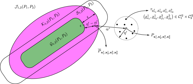
Figure 4: The geometry of various sets of distributions in the converse proof in Section XIV-C1. We assume ${\mathcal{G}}_{{1,2}}\left(P_{1},P_{2}\right)\setminus{\mathcal{K}}_{{1,2}}\left(P_{1},P_{2}\right)=\emptyset$ and would like to show that any zero-error code pair has rate $R_{1}=0$ and $R_{2}=0$. In the above figure, the ambient space is the set ${\mathcal{J}}_{1,2}\left(P_{1},P_{2}\right)$ of self-couplings equipped with $\ell^{1}$ metric. The set ${\mathcal{G}}_{{1,2}}\left(P_{1},P_{2}\right)$ is a strict subset of ${\mathcal{K}}_{{1,2}}\left(P_{1},P_{2}\right)$ such that they are $\varepsilon$-separated (see Equation 87). The joint types of the equicoupled subcode pair $({\mathcal{C}}_{1}^{\prime},{\mathcal{C}}_{2}^{\prime})$ are in an $\eta^{\prime}$-ball (see Equation 91) around a distribution $P_{{\mathbf{x}}^{1}_{1},{\mathbf{x}}^{1}_{2},{\mathbf{x}}^{2}_{1},{\mathbf{x}}^{2}_{2}}$ which is assumed to be $\alpha$-symmetric (see Equation 86). We then project $P_{{\mathbf{x}}^{1}_{1},{\mathbf{x}}^{1}_{2},{\mathbf{x}}^{2}_{1},{\mathbf{x}}^{2}_{2}}$ to obtain a symmetric distribution $\overline{P}_{{\mathbf{x}}^{1}_{1},{\mathbf{x}}^{1}_{2},{\mathbf{x}}^{2}_{1},{\mathbf{x}}^{2}_{2}}$ defined in Equation 88. (Note that $\overline{P}_{{\mathbf{x}}^{1}_{1},{\mathbf{x}}^{1}_{2},{\mathbf{x}}^{2}_{1},{\mathbf{x}}^{2}_{2}}$ may be slight inside ${\mathcal{K}}_{{1,2}}\left(P_{1},P_{2}\right)$.) It can be shown that $P_{{\mathbf{x}}^{1}_{1},{\mathbf{x}}^{1}_{2},{\mathbf{x}}^{2}_{1},{\mathbf{x}}^{2}_{2}}$ and $\overline{P}_{{\mathbf{x}}^{1}_{1},{\mathbf{x}}^{1}_{2},{\mathbf{x}}^{2}_{1},{\mathbf{x}}^{2}_{2}}$ are $\alpha^{\prime}$-close (see Equation 89). Since $({\mathcal{C}}_{1}^{\prime},{\mathcal{C}}_{2}^{\prime})$ attains zero error and all joint types are outside ${\mathcal{K}}_{{1,2}}\left(P_{1},P_{2}\right)$, one can show that $\overline{P}_{{\mathbf{x}}^{1}_{1},{\mathbf{x}}^{1}_{2},{\mathbf{x}}^{2}_{1},{\mathbf{x}}^{2}_{2}}$ is $(\varepsilon-\eta^{\prime}-\alpha^{\prime})$-far from ${\mathcal{G}}_{{1,2}}\left(P_{1},P_{2}\right)$ (see 32). This allows us to proceed with the double counting argument.

We assume that ${\mathcal{G}}_{{1,2}}\left(P_{1},P_{2}\right)$ is a proper subset of ${\mathcal{K}}_{{1,2}}\left(P_{1},P_{2}\right)$. Specifically, we assume that there exists a constant $\varepsilon>0$ such that

$$d_{{1}}\left({\mathcal{G}}_{{1,2}}\left(P_{1},P_{2}\right),{\mathcal{J}}_{1,2}\left(P_{1},P_{2}\right)\setminus{\mathcal{K}}_{{1,2}}\left(P_{1},P_{2}\right)\right)\geq\varepsilon.$$ (87)

We first project $P_{{\mathbf{x}}^{1}_{1},{\mathbf{x}}^{1}_{2},{\mathbf{x}}^{2}_{1},{\mathbf{x}}^{2}_{2}}$ to ${\mathcal{S}}_{1,2}\left(P_{1},P_{2}\right)$ and obtain an exactly symmetric distribution $\overline{P}_{{\mathbf{x}}^{1}_{1},{\mathbf{x}}^{1}_{2},{\mathbf{x}}^{2}_{1},{\mathbf{x}}^{2}_{2}}$,

$$\overline{P}_{{\mathbf{x}}^{1}_{1},{\mathbf{x}}^{1}_{2},{\mathbf{x}}^{2}_{1},{\mathbf{x}}^{2}_{2}}\coloneqq\frac{1}{4}\left(P_{{\mathbf{x}}^{1}_{1},{\mathbf{x}}^{1}_{2},{\mathbf{x}}^{2}_{1},{\mathbf{x}}^{2}_{2}}+P_{{\mathbf{x}}^{1}_{2},{\mathbf{x}}^{1}_{1},{\mathbf{x}}^{2}_{1},{\mathbf{x}}^{2}_{2}}+P_{{\mathbf{x}}^{1}_{1},{\mathbf{x}}^{1}_{2},{\mathbf{x}}^{2}_{2},{\mathbf{x}}^{2}_{1}}+P_{{\mathbf{x}}^{1}_{2},{\mathbf{x}}^{1}_{1},{\mathbf{x}}^{2}_{2},{\mathbf{x}}^{2}_{1}}\right).$$ (88)

Since the four summands are all in ${\mathcal{J}}_{1,2}\left(P_{1},P_{2}\right)$, $\overline{P}_{{\mathbf{x}}^{1}_{1},{\mathbf{x}}^{1}_{2},{\mathbf{x}}^{2}_{1},{\mathbf{x}}^{2}_{2}}$ is also in ${\mathcal{J}}_{1,2}\left(P_{1},P_{2}\right)$. Also, one can easily check that it is indeed symmetric in the sense of Definition 14. Furthermore, $\overline{P}_{{\mathbf{x}}^{1}_{1},{\mathbf{x}}^{1}_{2},{\mathbf{x}}^{2}_{1},{\mathbf{x}}^{2}_{2}}$ and $P_{{\mathbf{x}}^{1}_{1},{\mathbf{x}}^{1}_{2},{\mathbf{x}}^{2}_{1},{\mathbf{x}}^{2}_{2}}$ are close to each other.

$$d_{{1}}\left(\overline{P}_{{\mathbf{x}}^{1}_{1},{\mathbf{x}}^{1}_{2},{\mathbf{x}}^{2}_{1},{\mathbf{x}}^{2}_{2}},P_{{\mathbf{x}}^{1}_{1},{\mathbf{x}}^{1}_{2},{\mathbf{x}}^{2}_{1},{\mathbf{x}}^{2}_{2}}\right)= \sum_{(x^{1}_{1},x^{1}_{2},x^{2}_{1},x^{2}_{2})\in{\mathcal{X}}_{1}^{2}\times{\mathcal{X}}_{2}^{2}}\left|\overline{P}_{{\mathbf{x}}^{1}_{1},{\mathbf{x}}^{1}_{2},{\mathbf{x}}^{2}_{1},{\mathbf{x}}^{2}_{2}}(x^{1}_{1},x^{1}_{2},x^{2}_{1},x^{2}_{2})-P_{{\mathbf{x}}^{1}_{1},{\mathbf{x}}^{1}_{2},{\mathbf{x}}^{2}_{1},{\mathbf{x}}^{2}_{2}}(x^{1}_{1},x^{1}_{2},x^{2}_{1},x^{2}_{2})\right|$$

$$\leq \sum_{(x^{1}_{1},x^{1}_{2},x^{2}_{1},x^{2}_{2})\in{\mathcal{X}}_{1}^{2}\times{\mathcal{X}}_{2}^{2}}\frac{1}{4}\left(\left|P_{{\mathbf{x}}^{1}_{1},{\mathbf{x}}^{1}_{2},{\mathbf{x}}^{2}_{1},{\mathbf{x}}^{2}_{2}}(x^{1}_{1},x^{1}_{2},x^{2}_{1},x^{2}_{2})-P_{{\mathbf{x}}^{1}_{2},{\mathbf{x}}^{1}_{1},{\mathbf{x}}^{2}_{1},{\mathbf{x}}^{2}_{2}}(x^{1}_{1},x^{1}_{2},x^{2}_{1},x^{2}_{2})\right|\right.$$

$$+\left|P_{{\mathbf{x}}^{1}_{1},{\mathbf{x}}^{1}_{2},{\mathbf{x}}^{2}_{1},{\mathbf{x}}^{2}_{2}}(x^{1}_{1},x^{1}_{2},x^{2}_{1},x^{2}_{2})-P_{{\mathbf{x}}^{1}_{1},{\mathbf{x}}^{1}_{2},{\mathbf{x}}^{2}_{2},{\mathbf{x}}^{2}_{1}}(x^{1}_{1},x^{1}_{2},x^{2}_{1},x^{2}_{2})\right|$$

$$+\left.\left|P_{{\mathbf{x}}^{1}_{1},{\mathbf{x}}^{1}_{2},{\mathbf{x}}^{2}_{1},{\mathbf{x}}^{2}_{2}}(x^{1}_{1},x^{1}_{2},x^{2}_{1},x^{2}_{2})-P_{{\mathbf{x}}^{1}_{2},{\mathbf{x}}^{1}_{1},{\mathbf{x}}^{2}_{2},{\mathbf{x}}^{2}_{1}}(x^{1}_{1},x^{1}_{2},x^{2}_{1},x^{2}_{2})\right|\right)$$

$$\leq \frac{3}{4}|{\mathcal{X}}_{1}|^{2}|{\mathcal{X}}_{2}|^{2}\alpha\eqqcolon\alpha^{\prime}.$$ (89)

Equation 89 follows from the assumption given by Equation 86. Though we will not use it, the above bound can be slightly improved to $\alpha^{\prime}=\frac{1}{4}\left(3|{\mathcal{X}}_{1}|^{2}|{\mathcal{X}}_{2}|^{2}-|{\mathcal{X}}_{1}||{\mathcal{X}}_{2}|^{2}-|{\mathcal{X}}_{1}|^{2}|{\mathcal{X}}_{2}|-|{\mathcal{X}}_{1}||{\mathcal{X}}_{2}|\right)$ by noting that some terms corresponding to ${\underline{x}}^{1}_{1}={\underline{x}}^{1}_{2}$ or ${\underline{x}}^{2}_{1}={\underline{x}}^{2}_{2}$ do not contributed to the sum.

Claim 32.

Under the assumptions of Section XIV-C1, $\overline{P}_{{\mathbf{x}}^{1}_{1},{\mathbf{x}}^{1}_{2},{\mathbf{x}}^{2}_{1},{\mathbf{x}}^{2}_{2}}$ is not in ${\mathcal{G}}_{{1,2}}\left(P_{1},P_{2}\right)$:

$$d_{{1}}\left(\overline{P}_{{\mathbf{x}}^{1}_{1},{\mathbf{x}}^{1}_{2},{\mathbf{x}}^{2}_{1},{\mathbf{x}}^{2}_{2}},{\mathcal{G}}_{{1,2}}\left(P_{1},P_{2}\right)\right)\geq \varepsilon-\eta^{\prime}-\alpha^{\prime},$$ (90)

where $\eta^{\prime}\coloneqq\left|{\mathcal{X}}_{1}\right|^{2}\left|{\mathcal{X}}_{2}\right|^{2}\eta$ and $\alpha^{\prime}$ was defined in Equation 89.

Proof.

To prove the claim, first recall that for any $1\leq i_{1}<i_{2}\leq M_{1}^{\prime}$ and $1\leq j_{1}<j_{2}\leq M_{2}^{\prime}$, we have (by 6)

$$d_{{1}}\left(\tau_{{\underline{x}}^{1}_{i_{1}},{\underline{x}}^{1}_{i_{2}},{\underline{x}}^{2}_{j_{1}},{\underline{x}}^{2}_{j_{2}}},P_{{\mathbf{x}}^{1}_{1},{\mathbf{x}}^{1}_{2},{\mathbf{x}}^{2}_{1},{\mathbf{x}}^{2}_{2}}\right)\leq \left|{\mathcal{X}}_{1}\right|^{2}\left|{\mathcal{X}}_{2}\right|^{2}d_{{\infty}}\left(\tau_{{\underline{x}}^{1}_{i_{1}},{\underline{x}}^{1}_{i_{2}},{\underline{x}}^{2}_{j_{1}},{\underline{x}}^{2}_{j_{2}}},P_{{\mathbf{x}}^{1}_{1},{\mathbf{x}}^{1}_{2},{\mathbf{x}}^{2}_{1},{\mathbf{x}}^{2}_{2}}\right)\leq\left|{\mathcal{X}}_{1}\right|^{2}\left|{\mathcal{X}}_{2}\right|^{2}\eta\eqqcolon\eta^{\prime}.$$ (91)

Since $({\mathcal{C}}_{1},{\mathcal{C}}_{2})$ is a good code pair, $({\mathcal{C}}_{1}^{\prime},{\mathcal{C}}_{2}^{\prime})$ is also good. Hence $\tau_{{\underline{x}}^{1}_{i_{1}},{\underline{x}}^{1}_{i_{2}},{\underline{x}}^{2}_{j_{1}},{\underline{x}}^{2}_{j_{2}}}$ is not confusable, i.e.,

$$\tau_{{\underline{x}}^{1}_{i_{1}},{\underline{x}}^{1}_{i_{2}},{\underline{x}}^{2}_{j_{1}},{\underline{x}}^{2}_{j_{2}}}\in{\mathcal{J}}_{1,2}\left(P_{1},P_{2}\right)\setminus{\mathcal{K}}_{{1,2}}\left(P_{1},P_{2}\right).$$ (92)

We get that $\tau_{{\underline{x}}^{1}_{i_{1}},{\underline{x}}^{1}_{i_{2}},{\underline{x}}^{2}_{j_{1}},{\underline{x}}^{2}_{j_{2}}}$ is strictly bounded away from ${\mathcal{G}}_{{1,2}}\left(P_{1},P_{2}\right)$.

$$d_{{1}}\left(\tau_{{\underline{x}}^{1}_{i_{1}},{\underline{x}}^{1}_{i_{2}},{\underline{x}}^{2}_{j_{1}},{\underline{x}}^{2}_{j_{2}}},{\mathcal{G}}_{{1,2}}\left(P_{1},P_{2}\right)\right)\geq d_{{1}}\left({\mathcal{G}}_{{1,2}}\left(P_{1},P_{2}\right),{\mathcal{J}}_{1,2}\left(P_{1},P_{2}\right)\setminus{\mathcal{K}}_{{1,2}}\left(P_{1},P_{2}\right)\right)\geq\varepsilon.$$ (93)

The first inequality is by Equation 92 and the second one follows from the assumption given by Equation 87. Equations 93 and 91 imply that $P_{{\mathbf{x}}^{1}_{1},{\mathbf{x}}^{1}_{2},{\mathbf{x}}^{2}_{1},{\mathbf{x}}^{2}_{2}}$ is strictly outside ${\mathcal{G}}_{{1,2}}\left(P_{1},P_{2}\right)$.

$$d_{{1}}\left(P_{{\mathbf{x}}^{1}_{1},{\mathbf{x}}^{1}_{2},{\mathbf{x}}^{2}_{1},{\mathbf{x}}^{2}_{2}},{\mathcal{G}}_{{1,2}}\left(P_{1},P_{2}\right)\right)\geq d_{{1}}\left(\tau_{{\underline{x}}^{1}_{i_{1}},{\underline{x}}^{1}_{i_{2}},{\underline{x}}^{2}_{j_{1}},{\underline{x}}^{2}_{j_{2}}},{\mathcal{G}}_{{1,2}}\left(P_{1},P_{2}\right)\right)-d_{{1}}\left(\tau_{{\underline{x}}^{1}_{i_{1}},{\underline{x}}^{1}_{i_{2}},{\underline{x}}^{2}_{j_{1}},{\underline{x}}^{2}_{j_{2}}},P_{{\mathbf{x}}^{1}_{1},{\mathbf{x}}^{1}_{2},{\mathbf{x}}^{2}_{1},{\mathbf{x}}^{2}_{2}}\right)\geq\varepsilon-\eta^{\prime}.$$ (94)

Combining Equations 94 and 89, we further have

$$d_{{1}}\left(\overline{P}_{{\mathbf{x}}^{1}_{1},{\mathbf{x}}^{1}_{2},{\mathbf{x}}^{2}_{1},{\mathbf{x}}^{2}_{2}},{\mathcal{G}}_{{1,2}}\left(P_{1},P_{2}\right)\right)\geq d_{{1}}\left(P_{{\mathbf{x}}^{1}_{1},{\mathbf{x}}^{1}_{2},{\mathbf{x}}^{2}_{1},{\mathbf{x}}^{2}_{2}},{\mathcal{G}}_{{1,2}}\left(P_{1},P_{2}\right)\right)-d_{{1}}\left(P_{{\mathbf{x}}^{1}_{1},{\mathbf{x}}^{1}_{2},{\mathbf{x}}^{2}_{1},{\mathbf{x}}^{2}_{2}},\overline{P}_{{\mathbf{x}}^{1}_{1},{\mathbf{x}}^{1}_{2},{\mathbf{x}}^{2}_{1},{\mathbf{x}}^{2}_{2}}\right)\geq\varepsilon-\eta^{\prime}-\alpha^{\prime}.$$

This finishes the proof of 32. ∎

Since $\overline{P}_{{\mathbf{x}}^{1}_{1},{\mathbf{x}}^{1}_{2},{\mathbf{x}}^{2}_{1},{\mathbf{x}}^{2}_{2}}\notin{\mathcal{G}}_{{1,2}}\left(P_{1},P_{2}\right)$ by Equation 90, we can apply Theorem 18. There exists $Q_{{\mathbf{x}}^{1}_{1},{\mathbf{x}}^{1}_{2},{\mathbf{x}}^{2}_{1},{\mathbf{x}}^{2}_{2}}\in\mathrm{co}\text{-}{\mathcal{G}}_{1,2}\left(P_{1},P_{2}\right)$ such that

$$\left\langle\overline{P}_{{\mathbf{x}}^{1}_{1},{\mathbf{x}}^{1}_{2},{\mathbf{x}}^{2}_{1},{\mathbf{x}}^{2}_{2}},Q_{{\mathbf{x}}^{1}_{1},{\mathbf{x}}^{1}_{2},{\mathbf{x}}^{2}_{1},{\mathbf{x}}^{2}_{2}}\right\rangle\leq -\varepsilon^{\prime}<0$$ (95)

for some constant $\varepsilon^{\prime}>0$.

To prove upper bounds on $M_{1}^{\prime}$ and $M_{2}^{\prime}$, the trick is to upper and lower bound the following quantity

$$\sum_{(i_{1},i_{2})\in[M_{1}^{\prime}]\times[M_{2}^{\prime}]}\sum_{(j_{1},j_{2})\in[M_{2}^{\prime}]\times[M_{2}^{\prime}]}\left\langle\tau_{{\underline{x}}^{1}_{i_{1}},{\underline{x}}^{1}_{i_{2}},{\underline{x}}^{2}_{j_{1}},{\underline{x}}^{2}_{j_{2}}},Q_{{\mathbf{x}}^{1}_{1},{\mathbf{x}}^{1}_{2},{\mathbf{x}}^{2}_{1},{\mathbf{x}}^{2}_{2}}\right\rangle.$$ (96)

Contrasting the upper and lower bounds on Equation 96 will give us an upper bound on $\max\left\{M_{1}^{\prime},M_{2}^{\prime}\right\}$. We first prove an upper bound on Equation 96.

Claim 33.

Equation 96 is at most

$$\sum_{(i_{1},i_{2})\in[M_{1}^{\prime}]\times[M_{2}^{\prime}]}\sum_{(j_{1},j_{2})\in[M_{2}^{\prime}]\times[M_{2}^{\prime}]}\left\langle\tau_{{\underline{x}}^{1}_{i_{1}},{\underline{x}}^{1}_{i_{2}},{\underline{x}}^{2}_{j_{1}},{\underline{x}}^{2}_{j_{2}}},Q_{{\mathbf{x}}^{1}_{1},{\mathbf{x}}^{1}_{2},{\mathbf{x}}^{2}_{1},{\mathbf{x}}^{2}_{2}}\right\rangle$$

$$\leq M_{1}^{\prime}(M_{1}^{\prime}-1)M_{2}^{\prime}(M_{2}^{\prime}-1)(\eta^{\prime}+\alpha^{\prime}-\varepsilon^{\prime})+M_{1}^{\prime 2}M_{2}^{\prime}+M_{1}^{\prime}M_{2}^{\prime 2}+M_{1}^{\prime}M_{2}^{\prime}.$$ (97)

Proof.

Expanding the summation in Equation 96, we have

$$\sum_{(i_{1},i_{2})\in[M_{1}^{\prime}]\times[M_{1}^{\prime}]}\sum_{(j_{1},j_{2})\in[M_{2}^{\prime}]\times[M_{2}^{\prime}]}\left\langle\tau_{{\underline{x}}^{1}_{i_{1}},{\underline{x}}^{1}_{i_{2}},{\underline{x}}^{2}_{j_{1}},{\underline{x}}^{2}_{j_{2}}},Q_{{\mathbf{x}}^{1}_{1},{\mathbf{x}}^{1}_{2},{\mathbf{x}}^{2}_{1},{\mathbf{x}}^{2}_{2}}\right\rangle$$

$$= \sum_{\begin{subarray}{c}(i_{1},i_{2},j_{1},j_{2})\in[M_{1}^{\prime}]^{2}\times[M_{2}^{\prime}]^{2}\\ i_{1}\neq i_{2},j_{1}\neq j_{2}\end{subarray}}+\sum_{\begin{subarray}{c}(i_{1},i_{2},j_{1},j_{2})\in[M_{1}^{\prime}]^{2}\times[M_{2}^{\prime}]^{2}\\ i_{1}=i_{2}\mathrm{\ or\ }j_{1}=j_{2}\end{subarray}}\left\langle\tau_{{\underline{x}}^{1}_{i_{1}},{\underline{x}}^{1}_{i_{2}},{\underline{x}}^{2}_{j_{1}},{\underline{x}}^{2}_{j_{2}}},Q_{{\mathbf{x}}^{1}_{1},{\mathbf{x}}^{1}_{2},{\mathbf{x}}^{2}_{1},{\mathbf{x}}^{2}_{2}}\right\rangle$$

$$= \sum_{i_{1}\neq i_{2},j_{1}\neq j_{2}}+\sum_{i_{1}\neq i_{2},j_{1}=j_{2}}+\sum_{i_{1}=i_{2},j_{1}\neq j_{2}}+\sum_{i_{1}=i_{2},j_{1}=j_{2}}\left\langle\tau_{{\underline{x}}^{1}_{i_{1}},{\underline{x}}^{1}_{i_{2}},{\underline{x}}^{2}_{j_{1}},{\underline{x}}^{2}_{j_{2}}},Q_{{\mathbf{x}}^{1}_{1},{\mathbf{x}}^{1}_{2},{\mathbf{x}}^{2}_{1},{\mathbf{x}}^{2}_{2}}\right\rangle.$$ (98)

Note that

$$\left\langle\tau_{{\underline{x}}^{1}_{i_{1}},{\underline{x}}^{1}_{i_{2}},{\underline{x}}^{2}_{j_{1}},{\underline{x}}^{2}_{j_{2}}},Q_{{\mathbf{x}}^{1}_{1},{\mathbf{x}}^{1}_{2},{\mathbf{x}}^{2}_{1},{\mathbf{x}}^{2}_{2}}\right\rangle\leq \left\|\tau_{{\underline{x}}^{1}_{i_{1}},{\underline{x}}^{1}_{i_{2}},{\underline{x}}^{2}_{j_{1}},{\underline{x}}^{2}_{j_{2}}}\right\|_{2}\left\|Q_{{\mathbf{x}}^{1}_{1},{\mathbf{x}}^{1}_{2},{\mathbf{x}}^{2}_{1},{\mathbf{x}}^{2}_{2}}\right\|_{2}\leq\left\|\tau_{{\underline{x}}^{1}_{i_{1}},{\underline{x}}^{1}_{i_{2}},{\underline{x}}^{2}_{j_{1}},{\underline{x}}^{2}_{j_{2}}}\right\|_{1}\left\|Q_{{\mathbf{x}}^{1}_{1},{\mathbf{x}}^{1}_{2},{\mathbf{x}}^{2}_{1},{\mathbf{x}}^{2}_{2}}\right\|_{1}=1.$$

The last three terms in Equation 98 is at most

$$M_{1}^{\prime 2}M_{2}^{\prime}+M_{1}^{\prime}M_{2}^{\prime 2}+M_{1}^{\prime}M_{2}^{\prime}.$$ (99)

The first term in Equation 98 can be bounded as follows.

$$\sum_{i_{1}\neq i_{2},j_{1}\neq j_{2}}\left\langle\tau_{{\underline{x}}^{1}_{i_{1}},{\underline{x}}^{1}_{i_{2}},{\underline{x}}^{2}_{j_{1}},{\underline{x}}^{2}_{j_{2}}},Q_{{\mathbf{x}}^{1}_{1},{\mathbf{x}}^{1}_{2},{\mathbf{x}}^{2}_{1},{\mathbf{x}}^{2}_{2}}\right\rangle$$

$$= \sum_{i_{1}\neq i_{2},j_{1}\neq j_{2}}\left(\left\langle\tau_{{\underline{x}}^{1}_{i_{1}},{\underline{x}}^{1}_{i_{2}},{\underline{x}}^{2}_{j_{1}},{\underline{x}}^{2}_{j_{2}}}-\overline{P}_{{\mathbf{x}}^{1}_{1},{\mathbf{x}}^{1}_{2},{\mathbf{x}}^{2}_{1},{\mathbf{x}}^{2}_{2}},Q_{{\mathbf{x}}^{1}_{1},{\mathbf{x}}^{1}_{2},{\mathbf{x}}^{2}_{1},{\mathbf{x}}^{2}_{2}}\right\rangle+\left\langle\overline{P}_{{\mathbf{x}}^{1}_{1},{\mathbf{x}}^{1}_{2},{\mathbf{x}}^{2}_{1},{\mathbf{x}}^{2}_{2}},Q_{{\mathbf{x}}^{1}_{1},{\mathbf{x}}^{1}_{2},{\mathbf{x}}^{2}_{1},{\mathbf{x}}^{2}_{2}}\right\rangle\right).$$ (100)

For any $i_{1}\neq i_{2}$ and $j_{1}\neq j_{2}$, the first term of the summand in Equation 100 is at most

$$\left\langle\tau_{{\underline{x}}^{1}_{i_{1}},{\underline{x}}^{1}_{i_{2}},{\underline{x}}^{2}_{j_{1}},{\underline{x}}^{2}_{j_{2}}}-\overline{P}_{{\mathbf{x}}^{1}_{1},{\mathbf{x}}^{1}_{2},{\mathbf{x}}^{2}_{1},{\mathbf{x}}^{2}_{2}},Q_{{\mathbf{x}}^{1}_{1},{\mathbf{x}}^{1}_{2},{\mathbf{x}}^{2}_{1},{\mathbf{x}}^{2}_{2}}\right\rangle\leq \left\|\tau_{{\underline{x}}^{1}_{i_{1}},{\underline{x}}^{1}_{i_{2}},{\underline{x}}^{2}_{j_{1}},{\underline{x}}^{2}_{j_{2}}}-\overline{P}_{{\mathbf{x}}^{1}_{1},{\mathbf{x}}^{1}_{2},{\mathbf{x}}^{2}_{1},{\mathbf{x}}^{2}_{2}}\right\|_{1}\left\|Q_{{\mathbf{x}}^{1}_{1},{\mathbf{x}}^{1}_{2},{\mathbf{x}}^{2}_{1},{\mathbf{x}}^{2}_{2}}\right\|_{\infty}$$ (101)

$$\leq d_{{1}}\left(\tau_{{\underline{x}}^{1}_{i_{1}},{\underline{x}}^{1}_{i_{2}},{\underline{x}}^{2}_{j_{1}},{\underline{x}}^{2}_{j_{2}}},P_{{\mathbf{x}}^{1}_{1},{\mathbf{x}}^{1}_{2},{\mathbf{x}}^{2}_{1},{\mathbf{x}}^{2}_{2}}\right)+d_{{1}}\left(P_{{\mathbf{x}}^{1}_{1},{\mathbf{x}}^{1}_{2},{\mathbf{x}}^{2}_{1},{\mathbf{x}}^{2}_{2}},\overline{P}_{{\mathbf{x}}^{1}_{1},{\mathbf{x}}^{1}_{2},{\mathbf{x}}^{2}_{1},{\mathbf{x}}^{2}_{2}}\right)$$ (102)

$$\leq \eta^{\prime}+\alpha^{\prime}.$$ (103)

In Equation 101, we used the symmetry (as per Definition 14) of $\overline{P}_{{\mathbf{x}}^{1}_{1},{\mathbf{x}}^{1}_{2},{\mathbf{x}}^{2}_{1},{\mathbf{x}}^{2}_{2}}$. Specifically, since $\overline{P}_{{\mathbf{x}}^{1}_{1},{\mathbf{x}}^{1}_{2},{\mathbf{x}}^{2}_{1},{\mathbf{x}}^{2}_{2}}\in{\mathcal{S}}_{1,2}\left(P_{1},P_{2}\right)$, we have

$$d_{{1}}\left(\tau_{{\underline{x}}^{1}_{i_{2}},{\underline{x}}^{1}_{i_{1}},{\underline{x}}^{2}_{j_{2}},{\underline{x}}^{2}_{j_{1}}},\overline{P}_{{\mathbf{x}}^{1}_{1},{\mathbf{x}}^{1}_{2},{\mathbf{x}}^{2}_{1},{\mathbf{x}}^{2}_{2}}\right)= d_{{1}}\left(\tau_{{\underline{x}}^{1}_{i_{1}},{\underline{x}}^{1}_{i_{2}},{\underline{x}}^{2}_{j_{1}},{\underline{x}}^{2}_{j_{2}}},\overline{P}_{{\mathbf{x}}^{1}_{2},{\mathbf{x}}^{1}_{1},{\mathbf{x}}^{2}_{2},{\mathbf{x}}^{2}_{1}}\right)=d_{{1}}\left(\tau_{{\underline{x}}^{1}_{i_{1}},{\underline{x}}^{1}_{i_{2}},{\underline{x}}^{2}_{j_{1}},{\underline{x}}^{2}_{j_{2}}},\overline{P}_{{\mathbf{x}}^{1}_{1},{\mathbf{x}}^{1}_{2},{\mathbf{x}}^{2}_{1},{\mathbf{x}}^{2}_{2}}\right),$$

$$d_{{1}}\left(\tau_{{\underline{x}}^{1}_{i_{2}},{\underline{x}}^{1}_{i_{1}},{\underline{x}}^{2}_{j_{1}},{\underline{x}}^{2}_{j_{2}}},\overline{P}_{{\mathbf{x}}^{1}_{1},{\mathbf{x}}^{1}_{2},{\mathbf{x}}^{2}_{1},{\mathbf{x}}^{2}_{2}}\right)= d_{{1}}\left(\tau_{{\underline{x}}^{1}_{i_{1}},{\underline{x}}^{1}_{i_{2}},{\underline{x}}^{2}_{j_{1}},{\underline{x}}^{2}_{j_{2}}},\overline{P}_{{\mathbf{x}}^{1}_{2},{\mathbf{x}}^{1}_{1},{\mathbf{x}}^{2}_{1},{\mathbf{x}}^{2}_{2}}\right)=d_{{1}}\left(\tau_{{\underline{x}}^{1}_{i_{1}},{\underline{x}}^{1}_{i_{2}},{\underline{x}}^{2}_{j_{1}},{\underline{x}}^{2}_{j_{2}}},\overline{P}_{{\mathbf{x}}^{1}_{1},{\mathbf{x}}^{1}_{2},{\mathbf{x}}^{2}_{1},{\mathbf{x}}^{2}_{2}}\right),$$

$$d_{{1}}\left(\tau_{{\underline{x}}^{1}_{i_{1}},{\underline{x}}^{1}_{i_{2}},{\underline{x}}^{2}_{j_{2}},{\underline{x}}^{2}_{j_{1}}},\overline{P}_{{\mathbf{x}}^{1}_{1},{\mathbf{x}}^{1}_{2},{\mathbf{x}}^{2}_{1},{\mathbf{x}}^{2}_{2}}\right)= d_{{1}}\left(\tau_{{\underline{x}}^{1}_{i_{1}},{\underline{x}}^{1}_{i_{2}},{\underline{x}}^{2}_{j_{1}},{\underline{x}}^{2}_{j_{2}}},\overline{P}_{{\mathbf{x}}^{1}_{1},{\mathbf{x}}^{1}_{2},{\mathbf{x}}^{2}_{2},{\mathbf{x}}^{2}_{1}}\right)=d_{{1}}\left(\tau_{{\underline{x}}^{1}_{i_{1}},{\underline{x}}^{1}_{i_{2}},{\underline{x}}^{2}_{j_{1}},{\underline{x}}^{2}_{j_{2}}},\overline{P}_{{\mathbf{x}}^{1}_{1},{\mathbf{x}}^{1}_{2},{\mathbf{x}}^{2}_{1},{\mathbf{x}}^{2}_{2}}\right).$$

Hence, the bound in Equation 103 holds for all $i_{1}\neq i_{2}$ and $j_{1}\neq j_{2}$ (not only for $i_{1}<i_{2}$ and $j_{1}<j_{2}$). In Equation 102, we used the trivial bound $\left\|Q_{{\mathbf{x}}^{1}_{1},{\mathbf{x}}^{1}_{2},{\mathbf{x}}^{2}_{1},{\mathbf{x}}^{2}_{2}}\right\|_{\infty}\leq 1$ since $Q_{{\mathbf{x}}^{1}_{1},{\mathbf{x}}^{1}_{2},{\mathbf{x}}^{2}_{1},{\mathbf{x}}^{2}_{2}}$ is a probability distribution. Equation 103 is by Equations 89 and 91. Combining Equations 103 and 95, we get that the first term in Equation 98 is at most

$$M_{1}^{\prime 2}M_{2}^{\prime 2}(\eta^{\prime}+\alpha^{\prime}-\varepsilon^{\prime}).$$ (104)

Overall, by Equations 99 and 104, we get an upper bound on Equation 96:

$$M_{1}^{\prime}(M_{1}^{\prime}-1)M_{2}^{\prime}(M_{2}^{\prime}-1)(\eta^{\prime}+\alpha^{\prime}-\varepsilon^{\prime})+M_{1}^{\prime 2}M_{2}^{\prime}+M_{1}^{\prime}M_{2}^{\prime 2}+M_{1}^{\prime}M_{2}^{\prime},$$

which completes the proof of 33. ∎

On the other hand, a lower bound on Equation 96 follows from a direct calculation.

Claim 34.

Equation 96 is nonnegative, i.e.,

$$\sum_{(i_{1},i_{2})\in[M_{1}^{\prime}]\times[M_{2}^{\prime}]}\sum_{(j_{1},j_{2})\in[M_{2}^{\prime}]\times[M_{2}^{\prime}]}\left\langle\tau_{{\underline{x}}^{1}_{i_{1}},{\underline{x}}^{1}_{i_{2}},{\underline{x}}^{2}_{j_{1}},{\underline{x}}^{2}_{j_{2}}},Q_{{\mathbf{x}}^{1}_{1},{\mathbf{x}}^{1}_{2},{\mathbf{x}}^{2}_{1},{\mathbf{x}}^{2}_{2}}\right\rangle\geq 0.$$ (105)

Proof.

We compute Equation 96 from the first principle and interchange the summations.

$$\sum_{(i_{1},i_{2})\in[M_{1}^{\prime}]\times[M_{2}^{\prime}]}\sum_{(j_{1},j_{2})\in[M_{2}^{\prime}]\times[M_{2}^{\prime}]}\left\langle\tau_{{\underline{x}}^{1}_{i_{1}},{\underline{x}}^{1}_{i_{2}},{\underline{x}}^{2}_{j_{1}},{\underline{x}}^{2}_{j_{2}}},Q_{{\mathbf{x}}^{1}_{1},{\mathbf{x}}^{1}_{2},{\mathbf{x}}^{2}_{1},{\mathbf{x}}^{2}_{2}}\right\rangle$$

$$= \sum_{(i_{1},i_{2})\in[M_{1}^{\prime}]^{2}}\sum_{(j_{1},j_{2})\in[M_{2}^{\prime}]^{2}}\sum_{(x^{1}_{1},x^{1}_{2})\in{\mathcal{X}}_{1}^{2}}\sum_{(x^{2}_{1},x^{2}_{2})\in{\mathcal{X}}_{2}^{2}}\tau_{{\underline{x}}^{1}_{i_{1}},{\underline{x}}^{1}_{i_{2}},{\underline{x}}^{2}_{j_{1}},{\underline{x}}^{2}_{j_{2}}}(x^{1}_{1},x^{1}_{2},x^{2}_{1},x^{2}_{2})Q(x^{1}_{1},x^{1}_{2},x^{2}_{1},x^{2}_{2})$$

$$= \sum_{\begin{subarray}{c}(x^{1}_{1},x^{1}_{2})\in{\mathcal{X}}_{1}^{2}\\ (x^{2}_{1},x^{2}_{2})\in{\mathcal{X}}_{2}^{2}\end{subarray}}\sum_{\begin{subarray}{c}(i_{1},i_{2})\in[M_{1}^{\prime}]^{2}\\ (j_{1},j_{2})\in[M_{2}^{\prime}]^{2}\end{subarray}}\frac{1}{n}\sum_{k\in[n]}\mathds{1}{\left\{{\underline{x}}^{1}_{i_{1}}(k)=x^{1}_{1}\right\}}\mathds{1}{\left\{{\underline{x}}^{1}_{i_{2}}(k)=x^{1}_{2}\right\}}\mathds{1}{\left\{{\underline{x}}^{2}_{j_{1}}(k)=x^{2}_{1}\right\}}\mathds{1}{\left\{{\underline{x}}^{2}_{j_{2}}(k)=x^{2}_{2}\right\}}Q(x^{1}_{1},x^{1}_{2},x^{2}_{1},x^{2}_{2})$$

$$= \frac{1}{n}\sum_{\begin{subarray}{c}(x^{1}_{1},x^{1}_{2})\in{\mathcal{X}}_{1}^{2}\\ (x^{2}_{1},x^{2}_{2})\in{\mathcal{X}}_{2}^{2}\end{subarray}}\sum_{k\in[n]}\left(\sum_{i_{1}\in[M_{1}^{\prime}]}\mathds{1}{\left\{{\underline{x}}^{1}_{i_{1}}(k)=x^{1}_{1}\right\}}\right)\left(\sum_{i_{2}\in[M_{1}^{\prime}]}\mathds{1}{\left\{{\underline{x}}^{1}_{i_{2}}(k)=x^{1}_{2}\right\}}\right)$$

$$\left(\sum_{j_{1}\in[M_{2}^{\prime}]}\mathds{1}{\left\{{\underline{x}}^{2}_{j_{1}}(k)=x^{2}_{1}\right\}}\right)\left(\sum_{j_{2}\in[M_{2}^{\prime}]}\mathds{1}{\left\{{\underline{x}}^{2}_{j_{2}}(k)=x^{2}_{2}\right\}}\right)Q(x^{1}_{1},x^{1}_{2},x^{2}_{1},x^{2}_{2})$$

$$= \frac{M_{1}^{\prime 2}M_{2}^{\prime 2}}{n}\sum_{k\in[n]}\sum_{\begin{subarray}{c}(x^{1}_{1},x^{1}_{2})\in{\mathcal{X}}_{1}^{2}\\ (x^{2}_{1},x^{2}_{2})\in{\mathcal{X}}_{2}^{2}\end{subarray}}P_{1}^{(k)}(x^{1}_{1})P_{1}^{(k)}(x^{1}_{2})P_{2}^{(k)}(x^{2}_{1})P_{2}^{(k)}(x^{2}_{2})Q(x^{1}_{1},x^{1}_{2},x^{2}_{1},x^{2}_{2})$$ (106)

$$= M_{1}^{\prime 2}M_{2}^{\prime 2}\left\langle\frac{1}{n}\sum_{k\in[n]}\left(P_{1}^{(k)}\right)^{\otimes 2}\otimes\left(P_{2}^{(k)}\right)^{\otimes 2},Q_{{\mathbf{x}}^{1}_{1},{\mathbf{x}}^{1}_{2},{\mathbf{x}}^{2}_{1},{\mathbf{x}}^{2}_{2}}\right\rangle$$

$$\geq 0.$$ (107)

In Equation 106, $P_{i}^{(k)}$ denotes the empirical distribution of the $k$-th column of the codebook ${\mathcal{C}}_{i}^{\prime}\in{\mathcal{X}}_{i}^{M_{i}^{\prime}\times n}$, i.e., for any $x^{i}\in{\mathcal{X}}_{i}$,

$$P_{i}^{(k)}(x^{i})=\frac{1}{M_{i}^{\prime}}\left|\left\{\ell\in[M_{i}^{\prime}]:{\underline{x}}^{i}_{\ell}(k)=x^{i}\right\}\right|.$$ (108)

Equation 107 follows from Theorem 18 since $\frac{1}{n}\sum_{k\in[n]}\left(P_{1}^{(k)}\right)^{\otimes 2}\otimes\left(P_{2}^{(k)}\right)^{\otimes 2}\in{\mathcal{G}}_{{1,2}}\left(P_{1},P_{2}\right)$ and $Q_{{\mathbf{x}}^{1}_{1},{\mathbf{x}}^{1}_{2},{\mathbf{x}}^{2}_{1},{\mathbf{x}}^{2}_{2}}\in\mathrm{co}\text{-}{\mathcal{G}}_{1,2}\left(P_{1},P_{2}\right)$.

This finishes the proof of 34. ∎

Finally, Equations 97 and 105 yield

$$0\leq M_{1}^{\prime 2}M_{2}^{\prime 2}(\eta^{\prime}+\alpha^{\prime}-\varepsilon^{\prime})+M_{1}^{\prime 2}M_{2}^{\prime}+M_{1}^{\prime}M_{2}^{\prime 2}+M_{1}^{\prime}M_{2}^{\prime}$$

$$\implies 0\leq M_{1}^{\prime}M_{2}^{\prime}(\eta^{\prime}+\alpha^{\prime}-\varepsilon^{\prime})+M_{1}^{\prime}+M_{2}^{\prime}+1$$

$$\implies 0\leq -\delta M^{\prime 2}+2M^{\prime}+1$$ (109)

$$\implies M^{\prime}\leq \frac{1+\sqrt{1+\delta}}{\delta}$$ (110)

In Equation 109, we let $M^{\prime}\coloneqq\max\left\{M_{1}^{\prime},M_{2}^{\prime}\right\}$ and $\delta\coloneqq\varepsilon^{\prime}-\eta^{\prime}-\alpha^{\prime}>0$. Equation 110 gives us the desired bound $\max\left\{M_{1}^{\prime},M_{2}^{\prime}\right\}\leq C$ for some constant $C>0$ independent of $n$.

XIV-C2 The case where ${\mathcal{G}}_{{1,2}}\left(P_{1},P_{2}\right)\setminus{\mathcal{K}}_{{1,2}}\left(P_{1},P_{2}\right)\neq\emptyset$

Intuitively, this case is impossible for the following reasons. In the last subsection, we have shown that for any of $|{\mathcal{C}}_{1}^{\prime}|$ and $|{\mathcal{C}}_{2}^{\prime}|$ to be large, the distribution $\overline{P}_{{\mathbf{x}}^{1}_{1},{\mathbf{x}}^{1}_{2},{\mathbf{x}}^{2}_{1},{\mathbf{x}}^{2}_{2}}$ should (approximately) belong to ${\mathcal{G}}_{{1,2}}\left(P_{1},P_{2}\right)\setminus{\mathcal{K}}_{{1,2}}\left(P_{1},P_{2}\right)$. For one thing, since $\overline{P}_{{\mathbf{x}}^{1}_{1},{\mathbf{x}}^{1}_{2},{\mathbf{x}}^{2}_{1},{\mathbf{x}}^{2}_{2}}\in{\mathcal{G}}_{{1}}\left(P_{1},P_{2}\right)$, by the second property in Proposition 17, $\left[\overline{P}_{{\mathbf{x}}^{1}_{1},{\mathbf{x}}^{1}_{2},{\mathbf{x}}^{2}_{1},{\mathbf{x}}^{2}_{2}}\right]_{{\mathbf{x}}^{1}_{1},{\mathbf{x}}^{1}_{2},{\mathbf{x}}^{2}_{1}}$ (approximately) belongs to ${\mathcal{G}}_{{1}}\left(P_{1},P_{2}\right)$ and $\left[\overline{P}_{{\mathbf{x}}^{1}_{1},{\mathbf{x}}^{1}_{2},{\mathbf{x}}^{2}_{1},{\mathbf{x}}^{2}_{2}}\right]_{{\mathbf{x}}^{1}_{1},{\mathbf{x}}^{2}_{1},{\mathbf{x}}^{2}_{2}}$ (approximately) belongs to ${\mathcal{G}}_{{2}}\left(P_{1},P_{2}\right)$. For another thing, since the code pair $({\mathcal{C}}_{1}^{\prime},{\mathcal{C}}_{2}^{\prime})$ is assumed to attain zero error in the first place, we have that $\left[\overline{P}_{{\mathbf{x}}^{1}_{1},{\mathbf{x}}^{1}_{2},{\mathbf{x}}^{2}_{1},{\mathbf{x}}^{2}_{2}}\right]_{{\mathbf{x}}^{1}_{1},{\mathbf{x}}^{1}_{2},{\mathbf{x}}^{2}_{1}}$ which is close to $\tau_{{\underline{x}}^{1}_{i_{1}},{\underline{x}}^{1}_{i_{2}},{\underline{x}}^{2}_{j_{1}}}$ is (approximately) outside ${\mathcal{K}}_{{1}}\left(P_{1},P_{2}\right)$ and $\left[\overline{P}_{{\mathbf{x}}^{1}_{1},{\mathbf{x}}^{1}_{2},{\mathbf{x}}^{2}_{1},{\mathbf{x}}^{2}_{2}}\right]_{{\mathbf{x}}^{1}_{1},{\mathbf{x}}^{2}_{1},{\mathbf{x}}^{2}_{2}}$ which is close to $\tau_{{\underline{x}}^{1}_{i_{1}},{\underline{x}}^{2}_{j_{1}},{\underline{x}}^{2}_{j_{2}}}$ is (approximately) outside ${\mathcal{K}}_{{2}}\left(P_{1},P_{2}\right)$. In summary, we found a distribution $\overline{P}_{{\mathbf{x}}^{1}_{1},{\mathbf{x}}^{1}_{2},{\mathbf{x}}^{2}}\in{\mathcal{G}}_{{1,2}}\left(P_{1},P_{2}\right)\setminus{\mathcal{K}}_{{1,2}}\left(P_{1},P_{2}\right)$ with $\left[\overline{P}_{{\mathbf{x}}^{1}_{1},{\mathbf{x}}^{1}_{2},{\mathbf{x}}^{2}_{1},{\mathbf{x}}^{2}_{2}}\right]_{{\mathbf{x}}^{1}_{1},{\mathbf{x}}^{1}_{2},{\mathbf{x}}^{2}_{1}}\in{\mathcal{G}}_{{1}}\left(P_{1},P_{2}\right)\setminus{\mathcal{K}}_{{1}}\left(P_{1},P_{2}\right)$ and $\left[\overline{P}_{{\mathbf{x}}^{1}_{1},{\mathbf{x}}^{1}_{2},{\mathbf{x}}^{2}_{1},{\mathbf{x}}^{2}_{2}}\right]_{{\mathbf{x}}^{1}_{1},{\mathbf{x}}^{2}_{1},{\mathbf{x}}^{2}_{2}}\in{\mathcal{G}}_{{2}}\left(P_{1},P_{2}\right)\setminus{\mathcal{K}}_{{2}}\left(P_{1},P_{2}\right)$. This, nevertheless, contradicts the assumption ${\mathcal{G}}\left(P_{1},P_{2}\right)=\emptyset$ of Item 1 in Theorem 20.

The above intuition can be formalized by taking a good care of various slack factors. We flesh out the details below.

In the previous section, we showed that for any constant $\gamma>0$, if the distribution $\overline{P}_{{\mathbf{x}}^{1}_{1},{\mathbf{x}}^{1}_{2},{\mathbf{x}}^{2}_{1},{\mathbf{x}}^{2}_{2}}$ (which is the symmetrized version of $P_{{\mathbf{x}}^{1}_{1},{\mathbf{x}}^{1}_{2},{\mathbf{x}}^{2}_{1},{\mathbf{x}}^{2}_{2}}$, as defined in Equation 88) associated to $({\mathcal{C}}_{1}^{\prime},{\mathcal{C}}_{2}^{\prime})$ is $\gamma$-far (in $\ell^{1}$ distance) from ${\mathcal{G}}_{{1,2}}\left(P_{1},P_{2}\right)$, then both $M_{1}^{\prime}$ and $M_{2}^{\prime}$ are at most a constant $g(\gamma)$ for some function $g(\gamma)\xrightarrow{\gamma\to 0}0$. In other words, for $M_{1}^{\prime}$ or $M_{2}^{\prime}$ to be sufficiently large, $\overline{P}_{{\mathbf{x}}^{1}_{1},{\mathbf{x}}^{1}_{2},{\mathbf{x}}^{2}_{1},{\mathbf{x}}^{2}_{2}}$ has to be $\gamma$-close (in $\ell^{1}$ distance) to ${\mathcal{G}}_{{1,2}}\left(P_{1},P_{2}\right)$ for an arbitrarily small constant $\gamma>0$. Note also that unlike $\tau_{{\underline{x}}^{1}_{i_{1}},{\underline{x}}^{1}_{i_{2}},{\underline{x}}^{2}_{j_{1}},{\underline{x}}^{2}_{j_{2}}}$, the distribution $\overline{P}_{{\mathbf{x}}^{1}_{1},{\mathbf{x}}^{1}_{2},{\mathbf{x}}^{2}_{1},{\mathbf{x}}^{2}_{2}}$ can be slightly inside ${\mathcal{K}}_{{1,2}}\left(P_{1},P_{2}\right)$. However, it cannot be significantly inside ${\mathcal{K}}_{{1,2}}\left(P_{1},P_{2}\right)$. Specifically, for any $1\leq i_{1}<i_{2}\leq M_{1}^{\prime}$ and $1\leq j_{1}<j_{2}\leq M_{2}^{\prime}$,

$$d_{{1}}\left(\overline{P}_{{\mathbf{x}}^{1}_{1},{\mathbf{x}}^{1}_{2},{\mathbf{x}}^{2}_{1},{\mathbf{x}}^{2}_{2}},{\mathcal{J}}_{1,2}\left(P_{1},P_{2}\right)\setminus{\mathcal{K}}_{{1,2}}\left(P_{1},P_{2}\right)\right)$$

$$\leq d_{{1}}\left(\overline{P}_{{\mathbf{x}}^{1}_{1},{\mathbf{x}}^{1}_{2},{\mathbf{x}}^{2}_{1},{\mathbf{x}}^{2}_{2}},P_{{\mathbf{x}}^{1}_{1},{\mathbf{x}}^{1}_{2},{\mathbf{x}}^{2}_{1},{\mathbf{x}}^{2}_{2}}\right)+d_{{1}}\left(P_{{\mathbf{x}}^{1}_{1},{\mathbf{x}}^{1}_{2},{\mathbf{x}}^{2}_{1},{\mathbf{x}}^{2}_{2}},\tau_{{\underline{x}}^{1}_{i_{1}},{\underline{x}}^{1}_{i_{2}},{\underline{x}}^{2}_{j_{1}},{\underline{x}}^{2}_{j_{2}}}\right)+d_{{1}}\left(\tau_{{\underline{x}}^{1}_{i_{1}},{\underline{x}}^{1}_{i_{2}},{\underline{x}}^{2}_{j_{1}},{\underline{x}}^{2}_{j_{2}}},{\mathcal{J}}_{1,2}\left(P_{1},P_{2}\right)\setminus{\mathcal{K}}_{{1,2}}\left(P_{1},P_{2}\right)\right)$$ (111)

$$\leq \alpha^{\prime}+\eta^{\prime}.$$ (112)

In Equation 112, we used Equations 89 and 91. Also, the last term in Equation 111 is zero due to Equation 92. Overall, we have that for any good code pair $({\mathcal{C}}_{1}^{\prime},{\mathcal{C}}_{1}^{\prime})\in{\mathcal{X}}_{1}^{M_{1}^{\prime}\times n}\times{\mathcal{X}}_{2}^{M_{2}^{\prime}\times n}$ extracted from Lemma 27, for either $M_{1}^{\prime}$ or $M_{2}^{\prime}$ to be sufficiently large, $\overline{P}_{{\mathbf{x}}^{1}_{1},{\mathbf{x}}^{1}_{2},{\mathbf{x}}^{2}_{1},{\mathbf{x}}^{2}_{2}}$ has to be $(\varepsilon-\eta^{\prime}-\alpha^{\prime})$-close to ${\mathcal{G}}_{{1,2}}\left(P_{1},P_{2}\right)$ and $(\alpha^{\prime}+\eta^{\prime})$-close to ${\mathcal{J}}_{1,2}\left(P_{1},P_{2}\right)\setminus{\mathcal{K}}_{{1,2}}\left(P_{1},P_{2}\right)$ for arbitrarily small constants $\varepsilon,\eta^{\prime},\alpha^{\prime}>0$.

Therefore, we can without loss of rigor drop these slack factors and assume for convenience

$$\overline{P}_{{\mathbf{x}}^{1}_{1},{\mathbf{x}}^{1}_{2},{\mathbf{x}}^{2}_{1},{\mathbf{x}}^{2}_{2}}\in{\mathcal{G}}_{{1,2}}\left(P_{1},P_{2}\right)\setminus{\mathcal{K}}_{{1,2}}\left(P_{1},P_{2}\right).$$ (113)

For this to be possible, in this subsection we consider the case where ${\mathcal{G}}_{{1,2}}\left(P_{1},P_{2}\right)\setminus{\mathcal{K}}_{{1,2}}\left(P_{1},P_{2}\right)\neq\emptyset$.

Let

$$\overline{P}_{{\mathbf{x}}^{1}_{1},{\mathbf{x}}^{1}_{2},{\mathbf{x}}^{2}}\coloneqq \left[\overline{P}_{{\mathbf{x}}^{1}_{1},{\mathbf{x}}^{1}_{2},{\mathbf{x}}^{2}_{1},{\mathbf{x}}^{2}_{2}}\right]_{{\mathbf{x}}^{1}_{1},{\mathbf{x}}^{1}_{2},{\mathbf{x}}^{2}_{1}}=\left[\overline{P}_{{\mathbf{x}}^{1}_{1},{\mathbf{x}}^{1}_{2},{\mathbf{x}}^{2}_{1},{\mathbf{x}}^{2}_{2}}\right]_{{\mathbf{x}}^{1}_{1},{\mathbf{x}}^{1}_{2},{\mathbf{x}}^{2}_{2}},$$

$$\overline{P}_{{\mathbf{x}}^{1},{\mathbf{x}}^{2}_{1},{\mathbf{x}}^{2}_{2}}\coloneqq \left[\overline{P}_{{\mathbf{x}}^{1}_{1},{\mathbf{x}}^{1}_{2},{\mathbf{x}}^{2}_{1},{\mathbf{x}}^{2}_{2}}\right]_{{\mathbf{x}}^{1}_{1},{\mathbf{x}}^{2}_{1},{\mathbf{x}}^{2}_{2}}=\left[\overline{P}_{{\mathbf{x}}^{1}_{1},{\mathbf{x}}^{1}_{2},{\mathbf{x}}^{2}_{1},{\mathbf{x}}^{2}_{2}}\right]_{{\mathbf{x}}^{1}_{2},{\mathbf{x}}^{2}_{1},{\mathbf{x}}^{2}_{2}}.$$

Since $\overline{P}_{{\mathbf{x}}^{1}_{1},{\mathbf{x}}^{1}_{2},{\mathbf{x}}^{2}_{1},{\mathbf{x}}^{2}_{2}}\in{\mathcal{G}}_{{1,2}}\left(P_{1},P_{2}\right)$, the equality of the respective marginals above is by the second property of Proposition 17. Furthermore, by Equation 112 and Lemma 9,

$$d_{{1}}\left(\overline{P}_{{\mathbf{x}}^{1}_{1},{\mathbf{x}}^{1}_{2},{\mathbf{x}}^{2}},{\mathcal{J}}_{1}\left(P_{1},P_{2}\right)\setminus{\mathcal{K}}_{{1}}\left(P_{1},P_{2}\right)\right)\leq \alpha^{\prime}+\eta^{\prime},$$ (114)

$$d_{{1}}\left(\overline{P}_{{\mathbf{x}}^{1},{\mathbf{x}}^{2}_{1},{\mathbf{x}}^{2}_{2}},{\mathcal{J}}_{2}\left(P_{1},P_{2}\right)\setminus{\mathcal{K}}_{{2}}\left(P_{1},P_{2}\right)\right)\leq \alpha^{\prime}+\eta^{\prime}.$$ (115)

We further divide the analysis into two cases (as shown in Figure 5).

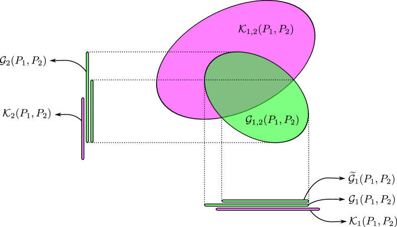
(a) The case where $\widetilde{{\mathcal{G}}_{{1}}}\left(P_{1},P_{2}\right)\setminus{\mathcal{K}}_{{1}}\left(P_{1},P_{2}\right)=\emptyset$ where $\widetilde{{\mathcal{G}}_{{1}}}\left(P_{1},P_{2}\right)$ is defined in Equation 116.

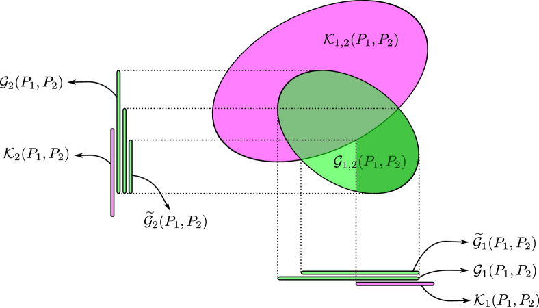
(b) The case where $\widetilde{{\mathcal{G}}_{{1}}}\left(P_{1},P_{2}\right)\setminus{\mathcal{K}}_{{1}}\left(P_{1},P_{2}\right)\neq\emptyset$ while $\widetilde{{\mathcal{G}}_{{2}}}\left(P_{1},P_{2}\right)\setminus{\mathcal{K}}_{{2}}\left(P_{1},P_{2}\right)=\emptyset$ where $\widetilde{{\mathcal{G}}_{{2}}}\left(P_{1},P_{2}\right)$ is defined in Equation 126.

Figure 5: Under the assumptions ${\mathcal{G}}\left(P_{1},P_{2}\right)=\emptyset$ and ${\mathcal{G}}_{{1,2}}\left(P_{1},P_{2}\right)\setminus{\mathcal{K}}_{{1,2}}\left(P_{1},P_{2}\right)\neq\emptyset$, we further divide the converse analysis into two cases. The goal is to show that in these cases there do not exist zero-error code pairs of rates $R_{1}>0$ and $R_{2}>0$. In the above figures, pink sets are confusability sets and green sets are sets of good distributions. Two-dimensional sets are sets of joint distributions (e.g., ${\mathcal{G}}_{{1,2}}\left(P_{1},P_{2}\right),{\mathcal{K}}_{{1,2}}\left(P_{1},P_{2}\right)$) and one-dimensional sets are sets of marginal distributions (e.g., ${\mathcal{G}}_{{1}}\left(P_{1},P_{2}\right),{\mathcal{G}}_{{2}}\left(P_{1},P_{2}\right),{\mathcal{K}}_{{1}}\left(P_{1},P_{2}\right),{\mathcal{K}}_{{2}}\left(P_{1},P_{2}\right)$, etc.).

1. Define

   $$\widetilde{{\mathcal{G}}_{{1}}}\left(P_{1},P_{2}\right)\coloneqq \left\{\left[P_{{\mathbf{x}}^{1}_{1},{\mathbf{x}}^{1}_{2},{\mathbf{x}}^{2}_{1},{\mathbf{x}}^{2}_{2}}\right]_{{\mathbf{x}}^{1}_{1},{\mathbf{x}}^{1}_{2},{\mathbf{x}}^{2}_{1}}:P_{{\mathbf{x}}^{1}_{1},{\mathbf{x}}^{1}_{2},{\mathbf{x}}^{2}_{1},{\mathbf{x}}^{2}_{2}}\in{\mathcal{G}}_{{1,2}}\left(P_{1},P_{2}\right)\setminus{\mathcal{K}}_{{1,2}}\left(P_{1},P_{2}\right)\right\}\subseteq{\mathcal{G}}_{{1}}\left(P_{1},P_{2}\right).$$ (116)

   Note that by Equation 113,

   $$\overline{P}_{{\mathbf{x}}^{1}_{1},{\mathbf{x}}^{1}_{2},{\mathbf{x}}^{2}}\in\widetilde{{\mathcal{G}}_{{1}}}\left(P_{1},P_{2}\right).$$ (117)

   Since we assume ${\mathcal{G}}\left(P_{1},P_{2}\right)=\emptyset$ in Item 1 of Theorem 20, $\widetilde{{\mathcal{G}}_{{1}}}\left(P_{1},P_{2}\right)\setminus{\mathcal{K}}_{{1}}\left(P_{1},P_{2}\right)$ may or may not be empty. We first handle the case where $\widetilde{{\mathcal{G}}_{{1}}}\left(P_{1},P_{2}\right)\setminus{\mathcal{K}}_{{1}}\left(P_{1},P_{2}\right)=\emptyset$. In fact, let us assume

   $$d_{{1}}\left(\widetilde{{\mathcal{G}}_{{1}}}\left(P_{1},P_{2}\right),{\mathcal{J}}_{1}\left(P_{1},P_{2}\right)\setminus{\mathcal{K}}_{{1}}\left(P_{1},P_{2}\right)\right)\geq\varepsilon_{1}$$ (118)

   for some $\varepsilon_{1}>0$. See Figure 5(a). However, Equations 117 and 114 lead to a contradiction if $\alpha^{\prime}$ and $\eta^{\prime}$ and sufficiently small so that $\alpha^{\prime}+\eta^{\prime}<\varepsilon_{1}$. Therefore, it is impossible for this case to happen.

2. Now we assume

   $$\widetilde{{\mathcal{G}}_{{1}}}\left(P_{1},P_{2}\right)\setminus{\mathcal{K}}_{{1}}\left(P_{1},P_{2}\right)\neq\emptyset.$$ (119)

   The analysis of the above case shows that $\overline{P}_{{\mathbf{x}}^{1}_{1},{\mathbf{x}}^{1}_{2},{\mathbf{x}}^{2}}\in\widetilde{{\mathcal{G}}_{{1}}}\left(P_{1},P_{2}\right)$ has to be $(\alpha^{\prime}+\eta^{\prime})$-close to ${\mathcal{J}}_{1}\left(P_{1},P_{2}\right)\setminus{\mathcal{K}}_{{1}}\left(P_{1},P_{2}\right)$ for arbitrarily small $\alpha^{\prime}$ and $\eta^{\prime}$. Similar to the assumption given by Equation 113, in the present case we may as well assume for convenience

   $$\overline{P}_{{\mathbf{x}}^{1}_{1},{\mathbf{x}}^{1}_{2},{\mathbf{x}}^{2}}\in\widetilde{{\mathcal{G}}_{{1}}}\left(P_{1},P_{2}\right)\setminus{\mathcal{K}}_{{1}}\left(P_{1},P_{2}\right).$$ (120)

   Now define

   $$\widetilde{{\mathcal{G}}_{{2}}}\left(P_{1},P_{2}\right)\coloneqq \left\{\left[P_{{\mathbf{x}}^{1}_{1},{\mathbf{x}}^{1}_{2},{\mathbf{x}}^{2}_{1},{\mathbf{x}}^{2}_{2}}\right]_{{\mathbf{x}}^{1}_{1},{\mathbf{x}}^{2}_{1},{\mathbf{x}}^{2}_{2}}:\begin{array}[]{rl}P_{{\mathbf{x}}^{1}_{1},{\mathbf{x}}^{1}_{2},{\mathbf{x}}^{2}_{1},{\mathbf{x}}^{2}_{2}}\in&{\mathcal{G}}_{{1,2}}\left(P_{1},P_{2}\right)\setminus{\mathcal{K}}_{{1,2}}\left(P_{1},P_{2}\right)\\ \left[P_{{\mathbf{x}}^{1}_{1},{\mathbf{x}}^{1}_{2},{\mathbf{x}}^{2}_{1},{\mathbf{x}}^{2}_{2}}\right]_{{\mathbf{x}}^{1}_{1},{\mathbf{x}}^{1}_{2},{\mathbf{x}}^{2}_{1}}\in&{\mathcal{G}}_{{1}}\left(P_{1},P_{2}\right)\setminus{\mathcal{K}}_{{1}}\left(P_{1},P_{2}\right)\end{array}\right\}$$ (123)

   $$= \left\{\left[P_{{\mathbf{x}}^{1}_{1},{\mathbf{x}}^{1}_{2},{\mathbf{x}}^{2}_{1},{\mathbf{x}}^{2}_{2}}\right]_{{\mathbf{x}}^{1}_{1},{\mathbf{x}}^{2}_{1},{\mathbf{x}}^{2}_{2}}:\begin{array}[]{rl}P_{{\mathbf{x}}^{1}_{1},{\mathbf{x}}^{1}_{2},{\mathbf{x}}^{2}_{1},{\mathbf{x}}^{2}_{2}}\in&{\mathcal{G}}_{{1,2}}\left(P_{1},P_{2}\right)\setminus{\mathcal{K}}_{{1,2}}\left(P_{1},P_{2}\right)\\ \left[P_{{\mathbf{x}}^{1}_{1},{\mathbf{x}}^{1}_{2},{\mathbf{x}}^{2}_{1},{\mathbf{x}}^{2}_{2}}\right]_{{\mathbf{x}}^{1}_{1},{\mathbf{x}}^{1}_{2},{\mathbf{x}}^{2}_{1}}\in&\widetilde{{\mathcal{G}}_{{1}}}\left(P_{1},P_{2}\right)\setminus{\mathcal{K}}_{{1}}\left(P_{1},P_{2}\right)\end{array}\right\}\subseteq{\mathcal{G}}_{{2}}\left(P_{1},P_{2}\right).$$ (126)

   Equation 126 is by Equation 116. By the assumption given by Equation 119, $\widetilde{{\mathcal{G}}_{{2}}}\left(P_{1},P_{2}\right)\neq\emptyset$. Note that by Equations 113 and 120,

   $$\overline{P}_{{\mathbf{x}}^{1},{\mathbf{x}}^{2}_{1},{\mathbf{x}}^{2}_{2}}\in\widetilde{{\mathcal{G}}_{{2}}}\left(P_{1},P_{2}\right).$$ (127)

   On the other hand, by the assumption ${\mathcal{G}}\left(P_{1},P_{2}\right)=\emptyset$ and Equation 119, $\widetilde{{\mathcal{G}}_{{2}}}\left(P_{1},P_{2}\right)\setminus{\mathcal{K}}_{{2}}\left(P_{1},P_{2}\right)$ must be empty. In fact let us assume

   $$d_{{1}}\left(\widetilde{{\mathcal{G}}_{{2}}}\left(P_{1},P_{2}\right),{\mathcal{J}}_{2}\left(P_{1},P_{2}\right)\setminus{\mathcal{K}}_{{2}}\left(P_{1},P_{2}\right)\right)\geq\varepsilon_{2}$$ (128)

   for some $\varepsilon_{2}>0$. See Figure 5(b). Now by Equations 115 and 127, we again reach a contradiction if $\alpha+\eta^{\prime}<\varepsilon_{2}$. Therefore, this case is also impossible to happen.

XV Converse, Items 2 and 3 in Theorem 20

In this section, we only prove Item 2. Item 3 follows by interchanging notation. We assume that ${\mathcal{G}}_{{1}}\left(P_{1},P_{2}\right)\setminus{\mathcal{K}}_{{1}}\left(P_{1},P_{2}\right)=\emptyset$. More precisely, we assume

$$d_{{1}}\left({\mathcal{G}}_{{1}}\left(P_{1},P_{2}\right),{\mathcal{J}}_{1}\left(P_{1},P_{2}\right)\setminus{\mathcal{K}}_{{1}}\left(P_{1},P_{2}\right)\right)\geq\varepsilon$$ (129)

for some $\varepsilon>0$. Let $({\mathcal{C}}_{1},{\mathcal{C}}_{2})$ be any good code pair. Suppose $R_{1}>0$. Our goal is to derive a contradiction.

XV-A Subcode extraction

Theorem 35 (Ramsey’s theorem [Wik21]).

Let ${\mathcal{K}}_{M}$ denote the (undirected) complete graph on $M$ vertices. Let $N\in{\mathbb{Z}}_{\geq 1},D\in{\mathbb{Z}}_{\geq 2}$. Then there exists a constant $K=K(N,D)$ such that for every $D$-coloring of the edges of ${\mathcal{K}}_{M}$ with $M\geq K$, there is a monochromatic clique in ${\mathcal{K}}_{M}$ of size at least $N$.

Lemma 36 (Subcode extraction).

Let $({\mathcal{C}}_{1},{\mathcal{C}}_{2})\subseteq{\mathcal{X}}_{1}^{n}\times{\mathcal{X}}_{2}^{n}$ be any $(P_{1},P_{2})$-constant composition code pair of sizes $M_{1},M_{2}$, respectively. Let $j\in[M_{2}]$. Then there exists a subcode ${\mathcal{C}}_{1}^{\prime}\subseteq{\mathcal{C}}$ of size $M_{1}^{\prime}\geq f(\left|{\mathcal{X}}_{1}\right|,\left|{\mathcal{X}}_{2}\right|,\eta,M_{1})\xrightarrow{M_{1}\to\infty}\infty$ and a distribution $P_{{\mathbf{x}}^{1}_{1},{\mathbf{x}}^{1}_{2},{\mathbf{x}}^{2}}\in{\mathcal{J}}_{1}\left(P_{1},P_{2}\right)$ such that for all $1\leq i_{1}<i_{1}\leq M_{1}^{\prime}$, we have $d_{{\infty}}\left(\tau_{{\underline{x}}^{1}_{i_{1}},{\underline{x}}^{1}_{i_{2}},{\underline{x}}^{2}_{j}},P_{{\mathbf{x}}^{1}_{1},{\mathbf{x}}^{1}_{2},{\mathbf{x}}^{2}}\right)\leq\eta$.

Proof.

The proof is similar to that of Lemma 27 and follows readily from Theorem 35. We first build a complete graph ${\mathcal{K}}_{M_{1}}$ whose vertex set is ${\mathcal{C}}_{1}$. We then color the edges of ${\mathcal{K}}_{M_{1}}$ using distributions in ${\mathcal{J}}_{1}\left(P_{1},P_{2}\right)$. Let ${\mathcal{N}}$ be an $\eta$-net of ${\mathcal{J}}_{1}\left(P_{1},P_{2}\right)$ of size at most $|{\mathcal{N}}|\leq\left(\frac{\left|{\mathcal{X}}_{1}\right|^{2}\times\left|{\mathcal{X}}_{2}\right|}{2\eta}+1\right)^{\left|{\mathcal{X}}_{1}\right|^{2}\times\left|{\mathcal{X}}_{2}\right|}\eqqcolon D$ (by Lemma 5). An edge $({\underline{x}}^{1}_{i_{1}},{\underline{x}}^{1}_{i_{2}})$ ($1\leq i_{1}<i_{2}\leq M_{1}$) is colored by a distribution $P_{{\mathbf{x}}^{1}_{1},{\mathbf{x}}^{1}_{2},{\mathbf{x}}^{2}}\in{\mathcal{N}}$ if $d_{{\infty}}\left(\tau_{{\underline{x}}^{1}_{i_{1}},{\underline{x}}^{1}_{i_{2}},{\underline{x}}^{2}_{j}},P_{{\mathbf{x}}^{1}_{1},{\mathbf{x}}^{1}_{2},{\mathbf{x}}^{2}}\right)\leq\eta$. Now by Theorem 35, there is a monochromatic subcode ${\mathcal{C}}_{1}^{\prime}\subseteq{\mathcal{C}}_{1}$ of size at least $M_{1}^{\prime}\geq f(\left|{\mathcal{X}}_{1}\right|,\left|{\mathcal{X}}_{2}\right|,\eta,M_{1})$, where $f(\left|{\mathcal{X}}_{1}\right|,\left|{\mathcal{X}}_{2}\right|,\eta,M_{1})\xrightarrow{M_{1}\to\infty}\infty$. According to the way we colored the edges, this means that for all $1\leq i_{1}<i_{2}\leq M_{1}^{\prime}$, $d_{{\infty}}\left(\tau_{{\underline{x}}^{1}_{i_{1}},{\underline{x}}^{1}_{i_{2}},{\underline{x}}^{2}_{j}},P_{{\mathbf{x}}^{1}_{1},{\mathbf{x}}^{1}_{2},{\mathbf{x}}^{2}}\right)\leq\eta$. ∎

Fix any $j\in[M_{2}]$. By Lemma 36, there is a subcode ${\mathcal{C}}_{1}^{\prime}\subseteq{\mathcal{C}}_{1}$ of size $M_{1}^{\prime}\xrightarrow{M_{1}\to\infty}\infty$ such that for some distribution $P_{{\mathbf{x}}^{1}_{1},{\mathbf{x}}^{1}_{2},{\mathbf{x}}^{2}}\in{\mathcal{J}}_{1}\left(P_{1},P_{2}\right)$, we have

$$d_{{\infty}}\left(\tau_{{\underline{x}}^{1}_{i_{1}},{\underline{x}}^{1}_{i_{2}},{\underline{x}}^{2}_{j}},P_{{\mathbf{x}}^{1}_{1},{\mathbf{x}}^{1}_{2},{\mathbf{x}}^{2}}\right)\leq\eta$$ (130)

for all $1\leq i_{1}<i_{2}\leq M_{1}^{\prime}$. Equation 130 implies, by 6, that

$$d_{{1}}\left(\tau_{{\underline{x}}^{1}_{i_{1}},{\underline{x}}^{1}_{i_{2}},{\underline{x}}^{2}_{j}},P_{{\mathbf{x}}^{1}_{1},{\mathbf{x}}^{1}_{2},{\mathbf{x}}^{2}}\right)\leq\left|{\mathcal{X}}_{1}\right|^{2}\left|{\mathcal{X}}_{2}\right|\eta\eqqcolon\eta^{\prime}.$$ (131)

In the following two sections (Sections XV-B and XV-C) we treat the cases where $P_{{\mathbf{x}}^{1}_{1},{\mathbf{x}}^{1}_{2},{\mathbf{x}}^{2}}$ is (noticeably) asymmetric and (approximately) symmetric (in the sense of Definition 14) separately.

XV-B Asymmetric case

Reusing the proof for Cases (5) & (6) of Lemma 28 with ${\mathbf{z}}^{2}$ being ${\mathbf{x}}^{2}$ (instead of $({\mathbf{x}}^{2}_{1},{\mathbf{x}}^{2}_{2})$ as in Section XIV-B) and ${\boldsymbol{\zeta}}^{2}$ corresponding to ${\underline{x}}^{2}_{j}$ (instead of $({\underline{x}}^{2}_{j_{1}},{\underline{x}}^{2}_{j_{2}})$ as in Section XIV-B), we get that $\mathrm{asymm}(P_{{\mathbf{x}}^{1}_{1},{\mathbf{x}}^{1}_{2},{\mathbf{x}}^{2}})\leq\alpha$ as long as $M_{1}^{\prime}\geq 36/(\alpha-4\sqrt{\eta}-2\eta)^{2}$.

XV-C Symmetric case

As we saw in the last section, for $M_{1}^{\prime}$ to be sufficiently large, $\mathrm{asymm}(P_{{\mathbf{x}}^{1}_{1},{\mathbf{x}}^{1}_{2},{\mathbf{x}}^{2}})\leq\alpha$. Under such an approximate symmetry condition, we then pass to an exactly symmetric distribution $\overline{P}_{{\mathbf{x}}^{1}_{1},{\mathbf{x}}^{1}_{2},{\mathbf{x}}^{2}}\in{\mathcal{S}}_{1}\left(P_{1},P_{2}\right)$ defined as

$$\overline{P}_{{\mathbf{x}}^{1}_{1},{\mathbf{x}}^{1}_{2},{\mathbf{x}}^{2}}\coloneqq \frac{1}{2}\left(P_{{\mathbf{x}}^{1}_{1},{\mathbf{x}}^{1}_{2},{\mathbf{x}}^{2}}+P_{{\mathbf{x}}^{1}_{2},{\mathbf{x}}^{1}_{1},{\mathbf{x}}^{2}}\right).$$

Furthermore,

$$d_{{1}}\left(\overline{P}_{{\mathbf{x}}^{1}_{1},{\mathbf{x}}^{1}_{2},{\mathbf{x}}^{2}},P_{{\mathbf{x}}^{1}_{1},{\mathbf{x}}^{1}_{2},{\mathbf{x}}^{2}}\right)= \sum_{(x^{1}_{1},x^{1}_{2},x^{2})\in{\mathcal{X}}_{1}^{2}\times{\mathcal{X}}_{2}}\left|\overline{P}_{{\mathbf{x}}^{1}_{1},{\mathbf{x}}^{1}_{2},{\mathbf{x}}^{2}}(x^{1}_{1},x^{1}_{2},x^{2})-P_{{\mathbf{x}}^{1}_{1},{\mathbf{x}}^{1}_{2},{\mathbf{x}}^{2}}(x^{1}_{1},x^{1}_{2},x^{2})\right|$$

$$\leq \frac{1}{2}\sum_{(x^{1}_{1},x^{1}_{2},x^{2})\in{\mathcal{X}}_{1}^{2}\times{\mathcal{X}}_{2}}\left|P_{{\mathbf{x}}^{1}_{2},{\mathbf{x}}^{1}_{1},{\mathbf{x}}^{2}}(x^{1}_{1},x^{1}_{2},x^{2})-P_{{\mathbf{x}}^{1}_{1},{\mathbf{x}}^{1}_{2},{\mathbf{x}}^{2}}(x^{1}_{1},x^{1}_{2},x^{2})\right|$$

$$\leq \frac{1}{2}\left|{\mathcal{X}}_{1}\right|^{2}\left|{\mathcal{X}}_{2}\right|\alpha\eqqcolon\alpha^{\prime}.$$ (132)

To apply the duality theorem (Theorem 18), we argue that $\overline{P}_{{\mathbf{x}}^{1}_{1},{\mathbf{x}}^{1}_{2},{\mathbf{x}}^{2}}$ is not in ${\mathcal{G}}_{{1}}\left(P_{1},P_{2}\right)$.

$$d_{{1}}\left(\overline{P}_{{\mathbf{x}}^{1}_{1},{\mathbf{x}}^{1}_{2},{\mathbf{x}}^{2}},{\mathcal{G}}_{{1}}\left(P_{1},P_{2}\right)\right)\geq d_{{1}}\left(P_{{\mathbf{x}}^{1}_{1},{\mathbf{x}}^{1}_{2},{\mathbf{x}}^{2}},{\mathcal{G}}_{{1}}\left(P_{1},P_{2}\right)\right)-d_{{1}}\left(P_{{\mathbf{x}}^{1}_{1},{\mathbf{x}}^{1}_{2},{\mathbf{x}}^{2}},\overline{P}_{{\mathbf{x}}^{1}_{1},{\mathbf{x}}^{1}_{2},{\mathbf{x}}^{2}}\right)$$

$$\geq d_{{1}}\left(\tau_{{\underline{x}}^{1}_{i_{1}},{\underline{x}}^{1}_{i_{2}},{\underline{x}}^{2}_{j}},{\mathcal{G}}_{{1}}\left(P_{1},P_{2}\right)\right)-d_{{1}}\left(\tau_{{\underline{x}}^{1}_{i_{1}},{\underline{x}}^{1}_{i_{2}},{\underline{x}}^{2}_{j}},P_{{\mathbf{x}}^{1}_{1},{\mathbf{x}}^{1}_{2},{\mathbf{x}}^{2}}\right)-\alpha^{\prime}$$ (133)

$$\geq d_{{1}}\left({\mathcal{G}}_{{1}}\left(P_{1},P_{2}\right),{\mathcal{J}}_{1}\left(P_{1},P_{2}\right)\setminus{\mathcal{K}}_{{1}}\left(P_{1},P_{2}\right)\right)-\eta^{\prime}-\alpha^{\prime}$$ (134)

$$\geq \varepsilon-\eta^{\prime}-\alpha^{\prime}.$$ (135)

Equation 133 is by Equation 132. Equation 134 is by Equation 131 and the fact that $\tau_{{\underline{x}}^{1}_{i_{1}},{\underline{x}}^{1}_{i_{2}},{\underline{x}}^{2}_{j}}\notin{\mathcal{K}}_{{1}}\left(P_{1},P_{2}\right)$. Equation 135 follows from Equation 129. By Theorem 18, there exists $Q_{{\mathbf{x}}^{1}_{1},{\mathbf{x}}^{1}_{2},{\mathbf{x}}^{2}}\in\mathrm{co}\text{-}{\mathcal{G}}_{1}\left(P_{1},P_{2}\right)$, such that

$$\left\langle\overline{P}_{{\mathbf{x}}^{1}_{1},{\mathbf{x}}^{1}_{2},{\mathbf{x}}^{2}},Q_{{\mathbf{x}}^{1}_{1},{\mathbf{x}}^{1}_{2},{\mathbf{x}}^{2}}\right\rangle\leq-\varepsilon^{\prime}$$ (136)

for some constant $\varepsilon^{\prime}>0$. The strategy is to bound

$$\sum_{(i_{1},i_{2})\in[M_{1}^{\prime}]^{2}}\left\langle\tau_{{\underline{x}}^{1}_{i_{1}},{\underline{x}}^{1}_{i_{2}},{\underline{x}}^{2}_{j}},Q_{{\mathbf{x}}^{1}_{1},{\mathbf{x}}^{1}_{2},{\mathbf{x}}^{2}}\right\rangle.$$ (137)

For an upper bound,

$$\sum_{(i_{1},i_{2})\in[M_{1}^{\prime}]^{2}}\left\langle\tau_{{\underline{x}}^{1}_{i_{1}},{\underline{x}}^{1}_{i_{2}},{\underline{x}}^{2}_{j}},Q_{{\mathbf{x}}^{1}_{1},{\mathbf{x}}^{1}_{2},{\mathbf{x}}^{2}}\right\rangle$$

$$= \sum_{\begin{subarray}{c}(i_{1},i_{2})\in[M_{1}^{\prime}]^{2}\\ i_{1}\neq i_{2}\end{subarray}}\left\langle\tau_{{\underline{x}}^{1}_{i_{1}},{\underline{x}}^{1}_{i_{2}},{\underline{x}}^{2}_{j}},Q_{{\mathbf{x}}^{1}_{1},{\mathbf{x}}^{1}_{2},{\mathbf{x}}^{2}}\right\rangle+\sum_{i\in[M_{1}^{\prime}]}\left\langle\tau_{{\underline{x}}^{1}_{i},{\underline{x}}^{1}_{i},{\underline{x}}^{2}_{j}},Q_{{\mathbf{x}}^{1}_{1},{\mathbf{x}}^{1}_{2},{\mathbf{x}}^{2}}\right\rangle$$

$$= \sum_{\begin{subarray}{c}(i_{1},i_{2})\in[M_{1}^{\prime}]^{2}\\ i_{1}\neq i_{2}\end{subarray}}\left(\left\langle\tau_{{\underline{x}}^{1}_{i_{1}},{\underline{x}}^{1}_{i_{2}},{\underline{x}}^{2}_{j}}-\overline{P}_{{\mathbf{x}}^{1}_{1},{\mathbf{x}}^{1}_{2},{\mathbf{x}}^{2}},Q_{{\mathbf{x}}^{1}_{1},{\mathbf{x}}^{1}_{2},{\mathbf{x}}^{2}}\right\rangle-\left\langle\overline{P}_{{\mathbf{x}}^{1}_{1},{\mathbf{x}}^{1}_{2},{\mathbf{x}}^{2}},Q_{{\mathbf{x}}^{1}_{1},{\mathbf{x}}^{1}_{2},{\mathbf{x}}^{2}}\right\rangle\right)+\sum_{i\in[M_{1}^{\prime}]}\left\langle\tau_{{\underline{x}}^{1}_{i},{\underline{x}}^{1}_{i},{\underline{x}}^{2}_{j}},Q_{{\mathbf{x}}^{1}_{1},{\mathbf{x}}^{1}_{2},{\mathbf{x}}^{2}}\right\rangle$$

$$\leq M_{1}^{\prime 2}(\eta^{\prime}+\alpha^{\prime}-\varepsilon^{\prime})+M_{1}^{\prime}.$$ (138)

In the above Equation 138, besides Equations 131, 132 and 136, we also used the fact that $\overline{P}_{{\mathbf{x}}^{1}_{1},{\mathbf{x}}^{1}_{2},{\mathbf{x}}^{2}}\in{\mathcal{S}}_{1}\left(P_{1},P_{2}\right)$ and hence by Definition 14

$$d_{{1}}\left(\tau_{{\underline{x}}^{1}_{i_{2}},{\underline{x}}^{1}_{i_{1}},{\underline{x}}^{2}_{j}},\overline{P}_{{\mathbf{x}}^{1}_{1},{\mathbf{x}}^{1}_{2},{\mathbf{x}}^{2}}\right)=d_{{1}}\left(\tau_{{\underline{x}}^{1}_{i_{1}},{\underline{x}}^{1}_{i_{2}},{\underline{x}}^{2}_{j}},\overline{P}_{{\mathbf{x}}^{1}_{2},{\mathbf{x}}^{1}_{1},{\mathbf{x}}^{2}}\right)=d_{{1}}\left(\tau_{{\underline{x}}^{1}_{i_{1}},{\underline{x}}^{1}_{i_{2}},{\underline{x}}^{2}_{j}},\overline{P}_{{\mathbf{x}}^{1}_{1},{\mathbf{x}}^{1}_{2},{\mathbf{x}}^{2}}\right).$$

For a lower bound,

$$\sum_{(i_{1},i_{2})\in[M_{1}^{\prime}]^{2}}\left\langle\tau_{{\underline{x}}^{1}_{i_{1}},{\underline{x}}^{1}_{i_{2}},{\underline{x}}^{2}_{j}},Q_{{\mathbf{x}}^{1}_{1},{\mathbf{x}}^{1}_{2},{\mathbf{x}}^{2}}\right\rangle$$

$$= \sum_{(i_{1},i_{2})\in[M_{1}^{\prime}]^{2}}\sum_{(x^{1}_{1},x^{1}_{2},x^{2})\in{\mathcal{X}}_{1}^{2}\times{\mathcal{X}}_{2}}\tau_{{\underline{x}}^{1}_{i_{1}},{\underline{x}}^{1}_{i_{2}},{\underline{x}}^{2}_{j}}(x^{1}_{1},x^{1}_{2},x^{2})Q_{{\mathbf{x}}^{1}_{1},{\mathbf{x}}^{1}_{2},{\mathbf{x}}^{2}}(x^{1}_{1},x^{1}_{2},x^{2})$$

$$= \sum_{(i_{1},i_{2})\in[M_{1}^{\prime}]^{2}}\sum_{(x^{1}_{1},x^{1}_{2},x^{2})\in{\mathcal{X}}_{1}^{2}\times{\mathcal{X}}_{2}}\frac{1}{n}\sum_{k\in[n]}\mathds{1}{\left\{{\underline{x}}^{1}_{i_{1}}(k)=x^{1}_{1},{\underline{x}}^{1}_{i_{2}}(k)=x^{1}_{2},{\underline{x}}^{2}_{j}(k)=x^{2}\right\}}Q_{{\mathbf{x}}^{1}_{1},{\mathbf{x}}^{1}_{2},{\mathbf{x}}^{2}}(x^{1}_{1},x^{1}_{2},x^{2})$$

$$= M_{1}^{\prime 2}\sum_{(x^{1}_{1},x^{1}_{2},x^{2})\in{\mathcal{X}}_{1}^{2}\times{\mathcal{X}}_{2}}\frac{1}{n}\sum_{k\in[n]}P_{1}^{(k)}(x^{1}_{1})P_{1}^{(k)}(x^{1}_{2})P_{2}^{(k)}(x^{2})Q_{{\mathbf{x}}^{1}_{1},{\mathbf{x}}^{1}_{2},{\mathbf{x}}^{2}}(x^{1}_{1},x^{1}_{2},x^{2})$$ (139)

$$= M_{1}^{\prime 2}\left\langle\frac{1}{n}\sum_{k\in[n]}\left(P_{1}^{(k)}\right)^{\otimes 2}\otimes P_{2}^{(k)},Q_{{\mathbf{x}}^{1}_{1},{\mathbf{x}}^{1}_{2},{\mathbf{x}}^{2}}\right\rangle\geq 0.$$ (140)

In Equation 139, $P_{1}^{(k)}$ denotes the empirical distribution of the $k$-th column of ${\mathcal{C}}_{1}^{\prime}$ as defined in Equation 108 for $i=1$; $P_{2}^{(k)}$ is the indicator distribution $P_{2}^{(k)}(x^{2})\coloneqq\mathds{1}{\left\{{\underline{x}}^{2}_{j}(k)=x^{2}\right\}}$ for all $x^{2}\in{\mathcal{X}}_{2}$. Equation 140 is by duality (Theorem 18).

Equations 138 and 140 jointly yield

$$M_{1}^{\prime 2}(\eta^{\prime}+\alpha^{\prime}-\varepsilon^{\prime})+M_{1}^{\prime}\geq 0,$$

i.e.,

$$M_{1}^{\prime}\leq \frac{1}{\varepsilon^{\prime}-\eta^{\prime}-\alpha^{\prime}}.$$

Remark 18.

The marginal cases (Items 2 and 3) of Theorem 20 proved in this section do not directly follow from the point-to-point results by Wang et al. [WBBJ19] in a black-box manner. Unlike in the achievability proof (see proofs of Items 2 and 3 of Lemma 22, proofs of Items 2 and 3 of Lemma 23 and proofs of Items 2 and 3 of Lemma 24), we cannot assume in a converse argument that a zero-rate codebook only contains one codeword. Indeed, a rateless code may contain subexponentially many codewords. Consequently, the adversary may leverage his knowledge of this small code and jam the communication in a potentially more malicious way than as if he was not aware of the existence of the small code (in which case the problem reduces to the point-to-point setting). Incorporating such strength of the adversary requires a more tender care of the converse argument as we did in this section.

Finally, we reiterate the nontriviality of the marginal cases of MACs even given the point-to-point results. Indeed, similar issues also arise in the study of AVMACs (where the adversary is oblivious) – another adversarial model that received more attention than ours over the past years. The corner cases where exactly one of the transmitters has zero capacity was left as a gap in Ahlswede and Cai’s paper [AC99], though the point-to-point results [Ahl78, CN88b] were known for long by then. The gap was later noticed by Wiese and Boche [WB12] and recently filled by Pereg and Steinberg [PS19], more than twenty years after [AC99].

XVI Concluding remarks and open problems

In the following remarks we reflect on the results we obtained and the techniques we leveraged in this paper, and interleave them with several promising/interesting open questions.

1. Another highly related yet different model that is not considered in this paper is the adversarial MACs with average probability of error. As briefly discussed in Remark 1, even for stochastic MACs, the capacity region exhibits different behaviours under average error criterion than maximum error criterion. Therefore, we do not believe that average error criterion behaves the same (at least under deterministic encoding) as the maximum one (which is equivalent to the zero error criterion under deterministic encoding) under our omniscient adversarial MAC model. Characterizing the capacity positivity and proving inner and outer bounds on the capacity region with average probability of error are left for future research. In contrast, for point-to-point AVCs, the capacity remains the same under average probability of error (with deterministic encoding) and maximum probability of error (with stochastic encoding) [CN88b].

2. For technical simplicity, this paper only handles deterministic MACs. For general (potentially stochastic) MACs, maximum error criterion is not equivalent to zero error criterion (though they are for deterministic MACs). Techniques along the lines of [CK81] are of relevance for extending our results to general adversarial MACs.

3. It is possible to generalize our results on capacity positivity to $t$-user MACs with $t>2$, though the case analysis may become baroque.

4. We believe that the capacity inner bounds obtained in Lemma 24 can be improved. In particular, the expurgation method we employed is crude – we expurgated one codeword from each user’s codebook for every pair of confusable pairs $(({\underline{\mathbf{x}}}^{1}_{i_{1}},{\underline{\mathbf{x}}}^{2}_{j_{1}}),({\underline{\mathbf{x}}}^{1}_{i_{2}},{\underline{\mathbf{x}}}^{2}_{j_{2}}))$. Noting that a pair of codewords $({\underline{\mathbf{x}}}^{1}_{i_{1}},{\underline{\mathbf{x}}}^{2}_{j_{1}})$ participates in $\Theta(M_{1}M_{2})$ many pairs $(({\underline{\mathbf{x}}}^{1}_{i_{1}},{\underline{\mathbf{x}}}^{2}_{j_{1}}),({\underline{\mathbf{x}}}^{1}_{i_{2}},{\underline{\mathbf{x}}}^{2}_{j_{2}}))$, we might have over-expurgated a more-than-desired number of codewords. We believe that more careful expurgation strategy may lead to improved inner bounds. For example, in [Gu18], a nontrivial lower bound for $t$-user binary adder MACs was obtained by only expurgating codewords with minimal violation of the zero error criterion. A naive expurgation as ours does not yield such a bound.

5. In classical zero-error information theory where channels under consideration are non-adversarial (or equivalently, unconstrainedly adversarial under our framework), there is a well-known $n$-letter expression for the capacity of a general DMC with zero error. The expression involves the independence number of the $n$-fold strong product of the confusability graph associated to the channel. Similarly, the non-stochastic information theory framework initiated by Nair [Nai11, Nai13] also provides multi-letter expressions in terms of non-stochastic information measures. In our opinion, the availability of such formulas heavily relies on the unconstrainedness of the channel. That is, viewed as an adversarial channel, the noise sequence ${\underline{s}}$ can take any value in ${\mathcal{S}}^{n}$. Consequently, “good codes tensorize” in the sense that if ${\mathcal{C}}\subseteq{\mathcal{X}}^{n}$ attains zero error then ${\mathcal{C}}\times{\mathcal{C}}\subseteq{\mathcal{X}}^{2n}$ also attains zero error. Unfortunately, such a tensorization property is not true for channels with state constraints. It can be easily seen that the adversary can allocate his power on the long codeword in a nonuniform manner so as to confuse the decoder. Codes for the adversarial bitflip channel is a concrete counterexample. The possibility of obtaining tight $n$-letter expressions for the capacity of omniscient adversarial channels using our framework is left for future investigations.

6. Recall that our main theorem asserts that for the sake of capacity positivity, it suffices to only consider distributions corresponding to mixtures of i.i.d. random variables. Achievability-wise, one can achieve positive rates, whenever possible, by sampling random codes using mixtures of product self-couplings, i.e., “good” distributions as per Definition 15. Conversely, if one could not achieve positive rates using good distributions, then she/he cannot achieve them using any other distributions. In the above sense, the set of good distributions we introduced plays a fundamental role in understanding capacity thresholds. This brings a natural question of whether there exist scenarios where correlated distributions help enlarge the region of positive rates and are hence also fundamentally “good”. One feasible way of physically instantiating correlation between input distributions is to allow cooperation. There is a recent line of works on oblivious adversarial MACs (i.e., the classical AVMAC model) with cooperation [WBBJ11, WB12, BS16, HS17]. That is, two encoders are allowed to communicate through a rate-limited channel. It is an interesting problem to examine the behaviour of MACs with cooperations under the omniscient model.

7. It is an intriguing question to extend our results to list decoding with constant list sizes. The list decoding problem for both (oblivious) AVCs [Hug97, SG12, BSP18, HK19, ZJB20] and AVMACs [BS16, Nit13, Cai16, Zha20] is well-studied. There are also papers on combinatorial list decoding for special MACs [DPSV19, Shc16], not mentioning a huge body of work on list decoding for bitflip channels. However, zero-error list decoding for general omniscient adversarial channels remains relatively uncharted until recently [ZBJ20]. One of the major technical challenges for MACs that is absent in the point-to-point case has to do with list configurations. A list for MAC can be represented by a bipartite graph [Cai16, Zha20]. For a target list size $L\in{\mathbb{Z}}_{\geq 2}$, the bipartite graph with $L$ edges corresponding to an $L$-list may have different “shapes”. Such complications call for delicate analysis.

8. It is plausible that our framework, built upon the prior work [WBBJ19], is eligible for tackling the capacity threshold problem of other adversarial multiuser channels, e.g., broadcast channels, interference channels, relay channels, etc. We leave this for further exploration. The non-adversarial/unconstrained version of these problems has been considered by Devroye [Dev16].

9. Motivated by the situation where the fundamental limit of oblivious MAC is well-understood [PS19] while that of the omniscient counterpart is out of reach of the current techniques, it is tempting to study an intermediate model which interpolates between the oblivious and the omniscient models. One model of this kind known as the myopic channels was initiated by Sarwate [Sar10] and was advanced in a sequence of followup work [DJL15, BDJ⁺20, ZVJS18]. Despite the progress, even the capacity threshold of general point-to-point myopic channels is unknown. In the case of MAC, one natural definition of the myopic variant could be that the adversary gets to observe a noisy version of the transmitted sequence pair through a stochastic (non-adversarial) MAC. Such a model, as far as we know, remains unexplored.

10. Strictly speaking, both our achievability and converse proofs rely on a strict separation between the set of good distributions and the confusability set. Specifically, we have to assume that the good set minus the confusability set has nonempty interior in the achievability proof; we have to assume that the good set is a proper subset of the confusability set in the converse proof. The case where the good set kisses the confusability set remains unsolved. Such boundary cases are solved for some special channels including the (point-to-point) bitflip channel (see, e.g., [GRS12, Theorem 4.4.1]). Similar subtleties also arise in the oblivious AVC/AVMAC setting where the boundary cases are in general open but are solved when the optimal jamming strategy is deterministic (which is the case, in particular, if the channel is deterministic) [CN88b, PS19]. In all above solved cases, the capacity is zero at the boundary. Inspired by these results, we conjecture that the capacity of our omniscient adversarial MACs is also zero in the boundary case. That is, our converse can be (conjecturally) strengthened.

11. Our proof heavily relies on the assumption of finite alphabets. It is unclear how to extend our proof to the case where the alphabet sizes grow with $n$. In fact, we believe that the behaviour of the capacity (region) is significantly different in the large alphabet regime. Indeed, for bitflip channels, there are algebraic constructions (notably the Reed–Solomon codes) attaining the capacity upper bound (the Singleton bound). In other words, unlike in the small alphabet case, the first-order asymptotics of bitflip channels are known as long as the alphabet sizes are sufficiently large (in particular at least $n$ suffices). It remains an intriguing question to explore the behaviour of omniscient adversarial MACs in the large alphabet regime.

12. Our converse results (Theorem 20) give upper bounds on the size of codes when the channel does not admit positive rates. For instance, if the set of good distributions is “$\varepsilon$-contained” (as per Equation 87) in the confusability set, then our proof gives $\max\left\{\left|{\mathcal{C}}_{1}\right|,\left|{\mathcal{C}}_{2}\right|\right\}\leq f(1/\varepsilon)$ which is independent of $n$. However, the function $f(\cdot)$ involves Ramsey number and is therefore enormous. We do not expect this bound to have an optimal dependence on $1/\varepsilon$. This type of question regarding the size of codes above the Plotkin bound was studied previously only for special channels. For instance, for the (point-to-point) bitflip channels with noise level $p$, the optimal dependence is known to be $\Theta(1/\varepsilon)$ [Lev61] where $\varepsilon=p-1/4$ is the gap between the Plotkin point and the noise level. Optimal bounds are also known for list decoding over bitflip channels with odd list sizes [ABP18]. We are not aware of any result on codes above the Plotkin bound for adversarial MACs.

XVII Acknowledgement

We thank Amitalok J. Budkuley and Sidharth Jaggi for many helpful discussions at the early stage of this work. We also thank Nir Ailon, Qi Cao and Chandra Nair for discussions on a related problem regarding zero-error binary adder MACs. This project has received funding from the European Union’s Horizon 2020 research and innovation programme under grant agreement No 682203-ERC-[Inf-Speed-Tradeoff].

Appendix A Table of notation

Frequently used notation is listed in the following table (LABEL:tab:notation).

TABLE IV: Table of frequently used notation.

Notation	Meaning	Definition
$\mathrm{asymm}_{1}(\cdot),\mathrm{asymm}_{2}(\cdot),\mathrm{asymm}_{1,2}(\cdot),\mathrm{asymm}(\cdot)$	Asymmetry of a joint distribution	Definition 19
$({\mathcal{C}}_{1},{\mathcal{C}}_{2})\subseteq{\mathcal{X}}_{1}^{n}\times{\mathcal{X}}_{2}^{n}$	Code pair	Definition 5
$\mathrm{co}\text{-}{\mathcal{G}}_{1}\left(P_{1},P_{2}\right),\mathrm{co}\text{-}{\mathcal{G}}_{2}\left(P_{1},P_{2}\right),\mathrm{co}\text{-}{\mathcal{G}}_{1,2}\left(P_{1},P_{2}\right)$	Sets of co-good tensors with marginals $(P_{1},P_{2})$	Definition 16
$\operatorname{Dec}\colon{\mathcal{Y}}^{n}\to[M_{1}]\times[M_{2}]$	Decoder of the receiver	Definition 5
$\operatorname{Enc}_{1}\colon[M_{1}]\to{\mathcal{X}}_{1}^{n},\operatorname{Enc}_{2}\colon[M_{2}]\to{\mathcal{X}}_{2}^{n}$	Encoders of the transmitters	Definition 5
${\mathcal{G}}_{{1}}\left(P_{1},P_{2}\right),{\mathcal{G}}_{{2}}\left(P_{1},P_{2}\right),{\mathcal{G}}_{{1,2}}\left(P_{1},P_{2}\right)$	Sets of good distributions with marginals $(P_{1},P_{2})$	Definition 15
${\mathcal{G}}\left(P_{1},P_{2}\right)$	Set of simultaneously good distributions with marginals $(P_{1},P_{2})$	Definition 15
${\mathcal{J}}_{1}\left(P_{1},P_{2}\right),{\mathcal{J}}_{2}\left(P_{1},P_{2}\right),{\mathcal{J}}_{1,2}\left(P_{1},P_{2}\right)$	Sets of self-couplings with marginals $(P_{1},P_{2})$	Definition 10
$\operatorname{Jam}\colon{\mathcal{X}}_{1}^{n}\times{\mathcal{X}}_{2}^{n}\to{\mathcal{S}}^{n}$	Jamming function of the adversary	Definition 6
${\mathcal{K}}_{{1}}\left(P_{1},P_{2}\right),{\mathcal{K}}_{{2}}\left(P_{1},P_{2}\right),{\mathcal{K}}_{{1,2}}\left(P_{1},P_{2}\right)$	Confusability sets with marginals $(P_{1},P_{2})$	Definition 11
$\mathsf{MAC}_{2}=\left({\mathcal{X}}_{1},{\mathcal{X}}_{2},{\mathcal{S}},{\mathcal{Y}},\Gamma_{1},\Gamma_{2},\Lambda,W_{{\mathbf{y}}|{\mathbf{x}},{\mathbf{s}}}\right)$	Omniscient adversarial MAC	Definition 4
$(m^{1},m^{2})\in[M_{1}]\times[M_{2}]$	Messages of the transmitters	Definition 4
$M_{1}=|{\mathcal{C}}_{1}|,M_{2}=|{\mathcal{C}}_{2}|$	Sizes of codebooks	Definition 5
$\left[P_{{\mathbf{x}},{\mathbf{y}}}\right]_{{\mathbf{x}}}\in\Delta({\mathcal{X}})$	Marginal distribution of $P_{{\mathbf{x}},{\mathbf{y}}}\in\Delta({\mathcal{X}}\times{\mathcal{Y}})$ on the variable ${\mathbf{x}}$	Section V
$(R_{1},R_{2})$	Rate pair	Definition 5
${\underline{s}}\in{\mathcal{S}}^{n}$	Jamming sequence of the adversary	Definition 4
${\mathcal{S}}$	Alphabet of the adversary	Definition 4
${\mathcal{S}}_{1}\left(P_{1},P_{2}\right),{\mathcal{S}}_{2}\left(P_{1},P_{2}\right),{\mathcal{S}}_{1,2}\left(P_{1},P_{2}\right)$	Sets of symmetric distributions with marginals $(P_{1},P_{2})$	Definition 14
$\mathsf{Sym}_{1}(P_{1},P_{2}),\mathsf{Sym}_{2}(P_{1},P_{2}),\mathsf{Sym}_{1,2}(P_{1},P_{2})$	Sets of symmetric tensors with marginals $(P_{1},P_{2})$	Definition 13
$W_{{\mathbf{y}}|{\mathbf{x}}^{1},{\mathbf{x}}^{2},{\mathbf{s}}}$	Channel transition law	Definition 4
$({\underline{x}}^{1},{\underline{x}}^{2})\in{\mathcal{X}}_{1}^{n}\times{\mathcal{X}}_{2}^{n}$	Input sequences from the transmitters	Definition 4
${\mathcal{X}}_{1},{\mathcal{X}}_{2}$	Alphabets of the transmitters	Definition 4
${\underline{y}}\in{\mathcal{Y}}^{n}$	Output sequence to the receiver	Definition 4
${\mathcal{Y}}$	Alphabet of the receiver	Definition 4
$(\Gamma_{1},\Gamma_{2})\subseteq\Delta({\mathcal{X}}_{1})\times\Delta({\mathcal{X}}_{2})$	Input constraints	Definition 4
$\Delta({\mathcal{X}})$	Probability simplex on ${\mathcal{X}}$	Section V
$\Delta_{1}(P_{1},P_{2}),\Delta_{2}(P_{1},P_{2}),\Delta_{1,2}(P_{1},P_{2})$	Sets of generalized self-couplings with marginals $(P_{1},P_{2})$	Definition 12
$\Delta^{(n)}({\mathcal{X}})$	Sets of types of ${\mathcal{X}}^{n}$-valued vectors	Definition 3
$\Lambda\subseteq\Delta({\mathcal{S}})$	State constraints	Definition 4
$\nu(P_{\mathbf{x}},n)$	–	Equation 1
$\tau_{{\underline{x}}}\in\Delta^{(n)}({\mathcal{X}})$	Type of ${\underline{x}}\in{\mathcal{X}}^{n}$	Definition 3

Appendix B Proof of Plotkin bound for binary noisy $\operatorname{\mathsf{XOR}}$ MACs (Theorem 11)

Proof of Theorem 11.

Suppose $p=1/4+\varepsilon$ for some constant $\varepsilon>0$. Let $\left({\mathcal{C}}_{1},{\mathcal{C}}_{2}\right)$ be a code pair which attains zero error on the binary noisy $\operatorname{\mathsf{XOR}}$ MAC. Let $M_{1}\coloneqq\left|{\mathcal{C}}_{1}\right|,M_{2}\coloneqq\left|{\mathcal{C}}_{2}\right|$. We will show that $M_{1}M_{2}\leq\nicefrac{{1}}{{4\varepsilon}}+1$. To this end, inspired the classical Plotkin bound in coding theory, we estimate the following quantity

$$\sum_{\left({\underline{x}}^{1}_{1},{\underline{x}}^{1}_{2},{\underline{x}}^{2}_{1},{\underline{x}}^{2}_{2}\right)\in{\mathcal{C}}_{1}^{2}\times{\mathcal{C}}_{2}^{2}}d_{\mathrm{H}}\left({\underline{x}}^{1}_{1}\oplus{\underline{x}}^{2}_{1},{\underline{x}}^{1}_{2}\oplus{\underline{x}}^{2}_{2}\right).$$ (141)

One the one hand, by the goodness of $({\mathcal{C}}_{1},{\mathcal{C}}_{2})$, as long as $({\underline{x}}^{1}_{1},{\underline{x}}^{2}_{1})\neq({\underline{x}}^{1}_{2},{\underline{x}}^{2}_{2})$, we have $d_{\mathrm{H}}\left({\underline{x}}^{1}_{1}\oplus{\underline{x}}^{2}_{1},{\underline{x}}^{1}_{2}\oplus{\underline{x}}^{2}_{2}\right)>2np$. For $({\underline{x}}^{1}_{1},{\underline{x}}^{2}_{1})=({\underline{x}}^{1}_{2},{\underline{x}}^{2}_{2})$, the summand is apparently zero. Therefore, Equation 141 is larger than $(M_{1}^{2}M_{2}^{2}-M_{1}M_{2})\cdot 2np$.

On the other hand, we can expand Equation 141 as follows.

$$\sum_{\left({\underline{x}}^{1}_{1},{\underline{x}}^{1}_{2},{\underline{x}}^{2}_{1},{\underline{x}}^{2}_{2}\right)\in{\mathcal{C}}_{1}^{2}\times{\mathcal{C}}_{2}^{2}}d_{\mathrm{H}}\left({\underline{x}}^{1}_{1}\oplus{\underline{x}}^{2}_{1},{\underline{x}}^{1}_{2}\oplus{\underline{x}}^{2}_{2}\right)$$

$$= \sum_{\left({\underline{x}}^{1}_{1},{\underline{x}}^{1}_{2},{\underline{x}}^{2}_{1},{\underline{x}}^{2}_{2}\right)\in{\mathcal{C}}_{1}^{2}\times{\mathcal{C}}_{2}^{2}}wt_{\mathrm{H}}\left({\underline{x}}^{1}_{1}\oplus{\underline{x}}^{2}_{1}\oplus{\underline{x}}^{1}_{2}\oplus{\underline{x}}^{2}_{2}\right)$$

$$= \sum_{\left({\underline{x}}^{1}_{1},{\underline{x}}^{1}_{2},{\underline{x}}^{2}_{1},{\underline{x}}^{2}_{2}\right)\in{\mathcal{C}}_{1}^{2}\times{\mathcal{C}}_{2}^{2}}\sum_{(a_{1},b_{1},a_{2},b_{2})\in{\mathcal{M}}}\sum_{j=1}^{n}\mathds{1}{\left\{{\underline{x}}^{1}_{1}(j)=a_{1}\right\}}\mathds{1}{\left\{{\underline{x}}^{2}_{1}(j)=b_{1}\right\}}\mathds{1}{\left\{{\underline{x}}^{1}_{2}(j)=a_{2}\right\}}\mathds{1}{\left\{{\underline{x}}^{2}_{2}(j)=b_{2}\right\}}$$ (142)

$$= \sum_{j=1}^{n}\sum_{(a_{1},b_{1},a_{2},b_{2})\in{\mathcal{M}}}\left(\sum_{{\underline{x}}^{1}_{1}\in{\mathcal{C}}_{1}}\mathds{1}{\left\{{\underline{x}}^{1}_{1}(j)=a_{1}\right\}}\right)\left(\sum_{{\underline{x}}^{2}_{1}\in{\mathcal{C}}_{2}}\mathds{1}{\left\{{\underline{x}}^{2}_{1}(j)=b_{1}\right\}}\right)\left(\sum_{{\underline{x}}^{1}_{2}\in{\mathcal{C}}_{1}}\mathds{1}{\left\{{\underline{x}}^{1}_{2}(j)=a_{2}\right\}}\right)\left(\sum_{{\underline{x}}^{2}_{2}\in{\mathcal{C}}_{2}}\mathds{1}{\left\{{\underline{x}}^{2}_{2}(j)=b_{2}\right\}}\right)$$

$$= \sum_{j=1}^{n}\big{(}(M_{1}-S_{j})(M_{2}-T_{j})(M_{1}-S_{j})T_{j}+(M_{1}-S_{j})(M_{2}-T_{j})S_{j}(M_{2}-T_{j})$$

$$+(M_{1}-S_{j})T_{j}(M_{1}-S_{j})(M_{2}-T_{j})+S_{j}(M_{2}-T_{j})(M_{1}-S_{j})(M_{2}-T_{j})$$

$$+S_{j}T_{j}S_{j}(M_{2}-T_{j})+S_{j}T_{j}(M_{1}-S_{j})T_{j}+S_{j}(M_{2}-T_{j})S_{j}T_{j}+(M_{1}-S_{j})T_{j}S_{j}T_{j}\big{)}$$ (143)

$$= M_{1}^{2}M_{2}^{2}\sum_{j=1}^{n}\left(\overline{\alpha}_{j}\overline{\beta}_{j}\overline{\alpha}_{j}\beta_{j}+\overline{\alpha}_{j}\overline{\beta}_{j}\alpha_{j}\overline{\beta}_{j}+\overline{\alpha}_{j}\beta_{j}\overline{\alpha}_{j}\overline{\beta}_{j}+\alpha_{j}\overline{\beta}_{j}\overline{\alpha}_{j}\overline{\beta}_{j}+\alpha_{j}\beta_{j}\alpha_{j}\overline{\beta}_{j}+\alpha_{j}\beta_{j}\overline{\alpha}_{j}\beta_{j}+\alpha_{j}\overline{\beta}_{j}\alpha_{j}\beta_{j}+\overline{\alpha}_{j}\beta_{j}\alpha_{j}\beta_{j}\right)$$ (144)

In Equation 142, we use ${\mathcal{M}}\coloneqq\left\{0001,0010,0100,1000,1110,1101,1011,0111\right\}$ to denote the set of length-4 binary sequences with odd parity. In Equation 143, we define $S_{j}\coloneqq\sum_{{\underline{x}}^{1}\in{\mathcal{C}}_{1}}\mathds{1}{\left\{{\underline{x}}^{1}(j)=1\right\}}$ and $T_{j}\coloneqq\sum_{{\underline{x}}^{2}\in{\mathcal{C}}_{2}}\mathds{1}{\left\{{\underline{x}}^{2}(j)=1\right\}}$ to be the number of 1’s in the $j$-th column of ${\mathcal{C}}_{1}\in\{0,1\}^{M_{1}\times n}$ and ${\mathcal{C}}_{2}\in\{0,1\}^{M_{2}\times n}$ respectively. In Equation 144, we further define $\alpha_{j}\coloneqq S_{j}/M_{1}$ and $\beta_{j}\coloneqq T_{j}/M_{2}$ to be the density of 1’s in the $j$-th column of ${\mathcal{C}}_{1}$ and ${\mathcal{C}}_{2}$ respectively; we also use the notation $\overline{a}\coloneqq 1-a$ for $a\in[0,1]$.

For any $j\in[n]$, since $\alpha_{j},\beta_{j}\in[0,1]$ the summand of Equation 144 is at most $1/2$. This can be verified by solving the following simple constrained (degree-4) polynomial optimization problem:

$$\max_{(\alpha,\beta)\in[0,1]^{2}}{\overline{\alpha}\overline{\beta}\overline{\alpha}\beta+\overline{\alpha}\overline{\beta}\alpha\overline{\beta}+\overline{\alpha}\beta\overline{\alpha}\overline{\beta}+\alpha\overline{\beta}\overline{\alpha}\overline{\beta}+\alpha\beta\alpha\overline{\beta}+\alpha\beta\overline{\alpha}\beta+\alpha\overline{\beta}\alpha\beta+\overline{\alpha}\beta\alpha\beta}.$$

The maximum $1/2$ is attained at $\alpha=1/4,\beta=1/2$. Therefore, Equation 141 is at most $M_{1}^{2}M_{2}^{2}n/2$.

Putting the lower and upper bounds on Equation 141 together, we have

$$\begin{array}[]{rrl}&\left(M_{1}^{2}M_{2}^{2}-{M_{1}M_{2}}\right)\cdot 2np<&\frac{M_{1}^{2}M_{2}^{2}n}{2}\\ \iff&\left(1-\frac{1}{M_{1}M_{2}}\right)2\left(\frac{1}{4}+\varepsilon\right)<&\frac{1}{2}\\ \iff&M_{1}M_{2}<&\frac{1}{4\varepsilon}+1,\end{array}$$

which finishes the proof of Theorem 11. ∎

References

- [ABP18] Noga Alon, Boris Bukh, and Yury Polyanskiy. List-decodable zero-rate codes. IEEE Transactions on Information Theory, 65(3):1657–1667, 2018.
- [AC99] Rudolf Ahlswede and Ning Cai. Arbitrarily varying multiple-access channels. i. ericson’s symmetrizability is adequate, gubner’s conjecture is true. IEEE Transactions on Information Theory, 45(2):742–749, 1999.
- [Ahl73] Rudolf Ahlswede. Multi-way communication channels. In Second International Symposium on Information Theory: Tsahkadsor, Armenia, USSR, Sept. 2-8, 1971, 1973.
- [Ahl74] Rudolf Ahlswede. The capacity region of a channel with two senders and two receivers. The annals of probability, 2(5):805–814, 1974.
- [Ahl78] R. Ahlswede. Elimination of correlation in random codes for arbitrarily varying channels. Z. Wahrscheinlichkeitstheorie Verv. Gebiete, 44:181–193, 1978.
- [AKKN17] Per Austrin, Petteri Kaski, Mikko Koivisto, and Jesper Nederlof. Sharper upper bounds for unbalanced uniquely decodable code pairs. IEEE Transactions on Information Theory, 64(2):1368–1373, 2017.
- [APBD18] Meysam Asadi, Kenneth Palacio-Baus, and Natasha Devroye. A relaying graph and special strong product for zero-error problems in primitive relay channels. In 2018 IEEE International Symposium on Information Theory (ISIT), pages 281–285. IEEE, 2018.
- [BDJ+20] Amitalok J Budkuley, Bikash Kumar Dey, Sidharth Jaggi, Michael Langberg, Anand D Sarwate, and Carol Wang. Symmetrizability for myopic avcs. In 2020 IEEE International Symposium on Information Theory (ISIT), pages 2103–2107. IEEE, 2020.
- [BLA76] LW BEINERE, BEINERE LW, and SCHWENK AJ. On a bipartite form of the ramsey problem. 1976.
- [BS16] Holger Boche and Rafael F Schaefer. Arbitrarily varying multiple access channels with conferencing encoders: List decoding and finite coordination resources. Advances in Mathematics of Communications, 10(2):333–354, 2016.
- [BSP18] Holger Boche, Rafael F Schaefer, and H Vincent Poor. Analytical properties of shannon’s capacity of arbitrarily varying channels under list decoding: Super-additivity and discontinuity behavior. Problems of Information Transmission, 54(3):199–228, 2018.
- [Cai16] Ning Cai. List decoding for arbitrarily varying multiple access channel revisited: List configuration and symmetrizability. IEEE Transactions on Information Theory, 62(11):6095–6110, 2016.
- [CD15] Yanying Chen and Natasha Devroye. On the optimality of colour-and-forward relaying for a class of zero-error primitive relay channels. In 2015 IEEE International Symposium on Information Theory (ISIT), pages 1272–1276. IEEE, 2015.
- [CD17] Yanying Chen and Natasha Devroye. Zero-error relaying for primitive relay channels. IEEE Transactions on Information Theory, 63(12):7708–7715, 2017.
- [CK81] I. Csiszár and J. Körner. On the capacity of the arbitrarily varying channel for maximum probability of error. Z. Wahrscheinlichkeitstheorie Verv. Gebiete, 57:87–101, 1981.
- [CK11] Imre Csiszár and János Körner. Information theory: coding theorems for discrete memoryless systems. Cambridge University Press, 2011.
- [CN88a] Imre Csiszár and Prakash Narayan. Arbitrarily varying channels with constrained inputs and states. IEEE Trans. Inf. Theory, 34:27–34, 1988.
- [CN88b] Imre Csiszár and Prakash Narayan. The Capacity of the Arbitrarily Varying Channel Revisited : Positivity, Constraints. IEEE Trans. Inf. Theory, 34:181–193, 1988.
- [CN91] Imre Csiszár and Prakash Narayan. Capacity of the gaussian arbitrarily varying channel. IEEE Transactions on Information Theory, 37(1):18–26, 1991.
- [Cov75] Thomas M Cover. Some advances in broadcast channels. In Advances in communication systems, volume 4, pages 229–260. Elsevier, 1975.
- [CSD14] Yanying Chen, Sara Shahi, and Natasha Devroye. Colour-and-forward: relaying “what the destination needs” in the zero-error primitive relay channel. In 2014 52nd Annual Allerton Conference on Communication, Control, and Computing (Allerton), pages 987–995. IEEE, 2014.
- [Csi98] Imre Csiszár. The method of types [information theory]. IEEE Transactions on Information Theory, 44(6):2505–2523, 1998.
- [Dev16] Natasha Devroye. When is the zero-error capacity positive in the relay, multiple-access, broadcast and interference channels? In 2016 54th Annual Allerton Conference on Communication, Control, and Computing (Allerton), pages 672–678. IEEE, 2016.
- [DJL15] Bikash Kumar Dey, Sidharth Jaggi, and Michael Langberg. Sufficiently myopic adversaries are blind. In Information Theory (ISIT), 2015 IEEE International Symposium on, pages 1164–1168, 2015.
- [DPSV19] Arkadii D’yachkov, Nikita Polyanskii, Vladislav Shchukin, and Ilya Vorobyev. Separable codes for the symmetric multiple-access channel. IEEE Transactions on Information Theory, 65(6):3738–3750, 2019.
- [Due78] G Dueck. Maximal error capacity regions are smaller than average error capacity regions for multi-user channels. 1978.
- [FN20] Farhad Farokhi and Girish Nair. Non-stochastic private function evaluation. arXiv preprint arXiv:2010.09968, 2020.
- [GGLR] L Gyorfi, Sándor Gyori, Bálint Laczay, and M Ruszinko. Lectures on multiple access channels. Web: http://www. szit. bme. hu/gyori/AFOSR, 5.
- [GH95] John A Gubner and Brian L Hughes. Nonconvexity of the capacity region of the multiple-access arbitrarily varying channel subject to constraints. IEEE transactions on information theory, 41(1):3–13, 1995.
- [GRS12] Venkatesan Guruswami, Atri Rudra, and Madhu Sudan. Essential coding theory. Draft available at http://www. cse. buffalo. edu/ atri/courses/coding-theory/book, 2012.
- [GS19] Yujie Gu and Ofer Shayevitz. On the non-adaptive zero-error capacity of the discrete memoryless two-way channel. In 2019 IEEE International Symposium on Information Theory (ISIT), pages 3107–3111. IEEE, 2019.
- [Gu18] Yuzhou Gu. Zero-error communication over adder mac. arXiv preprint arXiv:1809.07364, 2018.
- [HK19] Fatemeh Hosseinigoki and Oliver Kosut. List-decoding capacity of the gaussian arbitrarily-varying channel. Entropy, 21(6):575, 2019.
- [HS17] Wasim Huleihel and Yossef Steinberg. Channels with cooperation links that may be absent. IEEE Transactions on Information Theory, 63(9):5886–5906, 2017.
- [Hug97] Brian L. Hughes. The smallest list for the arbitrarily varying channel. IEEE Transactions on Information Theory, 43(3):803–815, 1997.
- [Kol56] Andrey Nikolaevich Kolmogorov. Certain asymptotic characteristics of completely bounded metric spaces. Doklady Akademii Nauk SSSR, 108(3):385–388, 1956.
- [Kom90] János Komlós. A strange pigeon-hole principle. Order, 7(2):107–113, 1990.
- [Kos20] Oliver Kosut. A second-order converse bound for the multiple-access channel via wringing dependence. arXiv preprint arXiv:2007.15664, 2020.
- [Lev61] VI Levenshtein. Application of hadamard matrices on coding problem. Problems of Cybernetica, 5:123–136, 1961.
- [LF17] Taehyung J Lim and Massimo Franceschetti. Information without rolling dice. IEEE Transactions on Information Theory, 63(3):1349–1363, 2017.
- [Lia72] HHJ Liao. Multiple Access Channels. Honolulu. PhD thesis, Ph. D. Dissertation, 1972.
- [Lov79] László Lovász. On the shannon capacity of a graph. IEEE Transactions on Information theory, 25(1):1–7, 1979.
- [Nai11] Girish N Nair. A non-stochastic information theory for communication and state estimation over erroneous channels. In 2011 9th IEEE International Conference on Control and Automation (ICCA), pages 159–164. IEEE, 2011.
- [Nai12] Girish N Nair. A nonstochastic information theory for feedback. In 2012 IEEE 51st IEEE Conference on Decision and Control (CDC), pages 1343–1348. IEEE, 2012.
- [Nai13] Girish N Nair. A nonstochastic information theory for communication and state estimation. IEEE Transactions on automatic control, 58(6):1497–1510, 2013.
- [Nit13] Sirin Nitinawarat. On the deterministic code capacity region of an arbitrarily varying multiple-access channel under list decoding. IEEE transactions on information theory, 59(5):2683–2693, 2013.
- [NY20] Chandra Nair and Mehdi Yazdanpanah. On the and-or interference channel and the sandglass conjecture. In 2020 IEEE International Symposium on Information Theory (ISIT), pages 1540–1545. IEEE, 2020.
- [PPV10] Yury Polyanskiy, H Vincent Poor, and Sergio Verdú. Channel coding rate in the finite blocklength regime. IEEE Transactions on Information Theory, 56(5):2307–2359, 2010.
- [PS19] Uzi Pereg and Yossef Steinberg. The capacity region of the arbitrarily varying mac: with and without constraints. In 2019 IEEE International Symposium on Information Theory (ISIT), pages 445–449. IEEE, 2019.
- [PW14] Yury Polyanskiy and Yihong Wu. Lecture notes on information theory. Lecture Notes for ECE563 (UIUC) and, 6(2012-2016):7, 2014.
- [RF19] Anshuka Rangi and Massimo Franceschetti. Towards a non-stochastic information theory. In 2019 IEEE International Symposium on Information Theory (ISIT), pages 997–1001. IEEE, 2019.
- [Sar10] Anand Sarwate. Coding against Myopic Adversaries. In Proc. IEEE Information Theory Workshop, Dublin, Ireland, 2010.
- [SFN18] Amir Saberi, Farhad Farokhi, and Girish Nair. Estimation and control over a nonstochastic binary erasure channel. IFAC-PapersOnLine, 51(23):265–270, 2018.
- [SFN19] Amir Saberi, Farhad Farokhi, and Girish N Nair. State estimation over worst-case erasure and symmetric channels with memory. arXiv preprint arXiv:1902.00726, 2019.
- [SFN20a] Amir Saberi, Farhad Farokhi, and Girish N Nair. Bounded state estimation over finite-state channels: Relating topological entropy and zero-error capacity. arXiv preprint arXiv:2003.11954, 2020.
- [SFN20b] Amir Saberi, Farhad Farokhi, and Girish N Nair. An explicit formula for the zero-error feedback capacity of a class of finite-state additive noise channels. arXiv preprint arXiv:2006.00892, 2020.
- [SG12] Anand D Sarwate and Michael Gastpar. List-decoding for the arbitrarily varying channel under state constraints. IEEE Transactions on Information Theory, 58(3):1372–1384, 2012.
- [Sha48] Claude E Shannon. A mathematical theory of communication. The Bell system technical journal, 27(3):379–423, 1948.
- [Sha56] Claude Shannon. The zero error capacity of a noisy channel. IRE Transactions on Information Theory, 2(3):8–19, 1956.
- [Sha61] Claude E Shannon. Two-way communication channels. In Proceedings of the Fourth Berkeley Symposium on Mathematical Statistics and Probability, Volume 1: Contributions to the Theory of Statistics. The Regents of the University of California, 1961.
- [Shc16] V Yu Shchukin. List decoding for a multiple access hyperchannel. Problems of Information Transmission, 52(4):329–343, 2016.
- [SMiF14] Jonathan Scarlett, Alfonso Martinez, and Albert Guillén i Fàbregas. Second-order rate region of constant-composition codes for the multiple-access channel. IEEE Transactions on Information Theory, 61(1):157–172, 2014.
- [SW73] David Slepian and Jack Keil Wolf. A coding theorem for multiple access channels with correlated sources. Bell System Technical Journal, 52(7):1037–1076, 1973.
- [Tik93] VM Tikhomirov. -entropy and -capacity of sets in functional spaces. In Selected works of AN Kolmogorov, pages 86–170. Springer, 1993.
- [TK13] Vincent YF Tan and Oliver Kosut. On the dispersions of three network information theory problems. IEEE Transactions on Information Theory, 60(2):881–903, 2013.
- [TT13] Marco Tomamichel and Vincent YF Tan. A tight upper bound for the third-order asymptotics for most discrete memoryless channels. IEEE Transactions on Information Theory, 59(11):7041–7051, 2013.
- [TT15] Vincent Yan Fu Tan and Marco Tomamichel. The third-order term in the normal approximation for the awgn channel. IEEE Transactions on Information Theory, 61(5):2430–2438, 2015.
- [WB12] Moritz Wiese and Holger Boche. The arbitrarily varying multiple-access channel with conferencing encoders. IEEE transactions on information theory, 59(3):1405–1416, 2012.
- [WBBJ11] Moritz Wiese, Holger Boche, Igor Bjelakovic, and Volker Jungnickel. The compound multiple access channel with partially cooperating encoders. IEEE transactions on information theory, 57(5):3045–3066, 2011.
- [WBBJ19] Xishi Wang, Amitalok J Budkuley, Andrej Bogdanov, and Sidharth Jaggi. When are large codes possible for avcs? In 2019 IEEE International Symposium on Information Theory (ISIT), pages 632–636. IEEE, 2019.
- [Wik21] Wikipedia contributors. Ramsey’s theorem — Wikipedia, the free encyclopedia, 2021. [Online; accessed 10-January-2021].
- [Wyn74] Aaron Wyner. Recent results in the shannon theory. IEEE Transactions on information Theory, 20(1):2–10, 1974.
- [YKE20] Recep Can Yavas, Victoria Kostina, and Michelle Effros. Gaussian multiple and random access in the finite blocklength regime. arXiv preprint arXiv:2001.03867, 2020.
- [ZBJ20] Yihan Zhang, Amitalok J Budkuley, and Sidharth Jaggi. Generalized list decoding. In 11th Innovations in Theoretical Computer Science Conference (ITCS 2020). Schloss Dagstuhl-Leibniz-Zentrum für Informatik, 2020.
- [Zha20] Yihan Zhang. List Decoding for Oblivious Arbitrarily Varying MACs: Constrained and Gaussian, 2020.
- [ZJB20] Yihan Zhang, Sidharth Jaggi, and Amitalok J Budkuley. Tight list-sizes for oblivious avcs under constraints. arXiv preprint arXiv:2009.03788, 2020.
- [ZN20] Ghassen Zafzouf and Girish N Nair. Distributed state estimation with bounded errors over multiple access channels. arXiv preprint arXiv:2002.03294, 2020.
- [ZNE19] Ghassen Zafzouf, Girish N Nair, and Jamie S Evans. Zero-error capacity of multiple access channels via nonstochastic information. In 2019 IEEE Information Theory Workshop (ITW), pages 1–5. IEEE, 2019.
- [ZVJ20] Yihan Zhang, Shashank Vatedka, and Sidharth Jaggi. Quadratically constrained two-way adversarial channels. arXiv preprint arXiv:2001.02575, 2020.
- [ZVJS18] Yihan Zhang, Shashank Vatedka, Sidharth Jaggi, and Anand D Sarwate. Quadratically constrained myopic adversarial channels. In 2018 IEEE International Symposium on Information Theory (ISIT), pages 611–615. IEEE, 2018.