Low Rank Forecasting

Abstract

We consider the problem of forecasting multiple values of the future of a vector time series, using some past values. This problem, and related ones such as one-step-ahead prediction, have a very long history, and there are a number of well-known methods for it, including vector auto-regressive models, state-space methods, multi-task regression, and others. Our focus is on low rank forecasters, which break forecasting up into two steps: estimating a vector that can be interpreted as a latent state, given the past, and then estimating the future values of the time series, given the latent state estimate. We introduce the concept of forecast consistency, which means that the estimates of the same value made at different times are consistent. We formulate the forecasting problem in general form, and focus on linear forecasters, for which we propose a formulation that can be solved via convex optimization. We describe a number of extensions and variations, including nonlinear forecasters, data weighting, the inclusion of auxiliary data, and additional objective terms. We illustrate our methods with several examples.

1 Introduction

Forecasting.

We consider the problem of forecasting future values of a vector time series $x_{t}\in{\mbox{\bf R}}^{n}$, $t=1,2,\ldots$, given previously observed values. At each time $t$ we form an estimate of the future values $x_{t+1},\ldots,x_{t+H}$, where $H$ is our prediction horizon. We denote these as $\hat{x}_{t+1|t},\hat{x}_{t+2|t},\ldots,\hat{x}_{t+H|t}$, where $\hat{x}_{\tau|t}$ is our prediction of $x_{\tau}$ made at time $t$. These estimates are based on the $M$ current and past values, $x_{t},x_{t-1},\ldots,x_{t-M+1}$, where $M$ is the memory of our forecaster. When $H=1$, forecasting reduces to the common problem of predicting the next value in the time series, given the previous $M$ values.

We introduce some notation to denote these windows of past and future values. We define the past at time $t$ as

$$p_{t}=(x_{t-M+1},\ldots,x_{t})\in{\mbox{\bf R}}^{Mn},\quad t=M,M+1,\ldots.$$

We define the future at time $t$ as

$$f_{t}=(x_{t+1},\ldots,x_{t+H})\in{\mbox{\bf R}}^{Hn},\quad t=1,2,\ldots.$$

We make the observation that $p_{t}$ and $p_{t+1}$ are related by a block shift, since

$$p_{t+1}=(x_{t-M+2},\ldots,x_{t+1})=((p_{t})_{n+1:Mn},x_{t+1}),$$

where $a_{i:j}$ denotes the subvector of $a$ with entries $i,\ldots,j$. A similar shift structure holds for $f_{t}$.

We use $\hat{f}_{t}$ to denote our estimate or forecast of the future at time $t$, i.e.,

$$\hat{f}_{t}=(\hat{x}_{t+1|t},\ldots,\hat{x}_{t+H|t})\in{\mbox{\bf R}}^{Hn}.$$

A forecaster has the form $\hat{f}_{t}=\phi(p_{t})$, and $\phi:{\mbox{\bf R}}^{Mn}\to{\mbox{\bf R}}^{Hn}$ defines the forecaster.

We observe that the forecasts do not necessarily have the shift structure that the past and future vectors do. While $(f_{t+1})_{1:n}$ and $(f_{t})_{n+1:2n}$ are both equal to $x_{t+2}$, $(\hat{f}_{t+1})_{1:n}$ and $(\hat{f}_{t})_{n+1:2n}$ can be different. The first is $\hat{x}_{t+2|t+1}$, our estimate of $x_{t+2}$ made at time $t+1$, whereas the second is $\hat{x}_{t+2|t}$, our estimate of $x_{t+2}$ made at time $t$. These two estimates need not be the same. (We will come back to this soon with the concept of forecasting consistency.)

Low rank forecasting and latent state.

We say that the forecaster has rank $r$ if the forecast function factors as $\phi=\mathcal{V}\circ\mathcal{U}$, where $\mathcal{U}:{\mbox{\bf R}}^{Mn}\to{\mbox{\bf R}}^{r}$ is the encoder and $\mathcal{V}:{\mbox{\bf R}}^{r}\to{\mbox{\bf R}}^{Hn}$ is the decoder, and $r\leq\min\{Mn,Hn\}$. This means that the forecast takes place in two steps: we first form the intermediate $r$-vector $z_{t}=\mathcal{U}(p_{t})$ by encoding the past, and then compute the forecast as $\hat{f}_{t}=\mathcal{V}(z_{t})$ by decoding $z_{t}$. We can interpret the time series $z_{t}$, $t=M,M+1,\ldots$ as a latent state. The term state is justified since $z_{t}$ is a summary of the past sufficient to carry out our forecast. Under Kalman’s definition, the state of a dynamic system is “the least amount of data one has to know about the past behavior of the system in order to predict its future behavior” [1]. (We note one small difference: In the traditional abstract definition of state, the past and future are infinite, whereas here we have limited them to $M$ and $H$ time periods, respectively.) The term rank for the dimension of the intermediate value $z_{t}$ is not standard; but we will see later that it coincides with the rank of a certain matrix when we restrict our attention to linear forecasters.

The latent state can be very useful in applications, since it summarizes what we need to know to about the past at time $t$ in one vector $z_{t}\in{\mbox{\bf R}}^{r}$, in order to carry out our forecast. In some applications, identifying the latent state can be just as important as carry out the actual forecasts.

Judging forecaster performance.

Suppose we have a $T$-long observation of the time series, $x_{1},\ldots,x_{T}$, with $T\geq M+H$. From this data set we extract the $N$ pairs of past and future,

$$(p_{M},f_{M}),\ldots,(p_{T-H},f_{T-H}),$$

with $N=T-H-M+1$. We judge the performance of a forecaster on this data set by its average loss,

$$\mathcal{L}=\frac{1}{N}\sum_{t=M}^{T-H}\ell(\hat{f}_{t}-f_{t}),$$

where $\ell:{\mbox{\bf R}}^{Hn}\to{\mbox{\bf R}}$ is a convex loss function. (The lower the loss function, the better the forecast.) Common choices include the $\ell_{2}$ (squared) loss $\ell(u)=\|u\|_{2}^{2}$, $\ell_{1}$ loss $\ell(u)=\|u\|_{1}$, or an appropriate Huber penalty function [2, §6.1.2].

When the data set is also the one used to fit or choose the forecaster, $\mathcal{L}$ is the training loss. When the data set is a different set of data, not used to fit or choose the forecaster, $\mathcal{L}$ is the test loss. We are interested in finding a forecaster that has low test loss, i.e., makes good forecasts on data that was not used to fit it. Another approach is walk-forward cross-validation, where one produces a number of successive training and test data sets from a single data set, where all test data points occur after all training data points. (This is to avoid look-ahead bias, and is in contrast to standard cross-validation, where one creates random training and test splits.)

Forecaster consistency.

Consider the value $x_{\tau}$, with $\tau\geq M+1$. We make predictions of $x_{\tau}$, denoted as $\hat{x}_{\tau|t}$, at times

$$t=\max\{\tau-H,M+1\},\ldots,\min\{\tau-1,T-H\}.$$

These

$$\min\{\tau,T-H+1\}-\max\{\tau-H,M+1\}=\left\{\begin{array}[]{ll}H&H+M+1\leq\tau\leq T-H+1,\\ \tau-M-1&\tau\leq\min\{T-H+1,H+M+1\},\\ T-\tau+1&\tau\geq\max\{T-H+1,H+M+1\},\\ T-H-M&\text{otherwise},\end{array}\right.$$

forecasts of the same value, made at different times and with different available information, need not be the same. We say the forecast is consistent if these forecasts are not too different. We note that inconsistency is not necessarily bad; it simply means that over the different periods in which we form a prediction of $x_{\tau}$, we are changing our prediction.

While other measures of inconsistency could be used, we will judge inconsistency of the forecasts of $x_{\tau}$ using a sum of squares measure. Define

$$\bar{x}_{\tau}=\frac{1}{\min\{\tau,T-H+1\}-\max\{\tau-H,M+1\}}\sum_{t=\max\{\tau-H,M+1\}}^{\min\{\tau-1,T-H\}}\hat{x}_{\tau|t},$$

the average of the predictions of $x_{\tau}$ made at different times. Thus $\hat{x}_{\tau|t}-\bar{x}_{\tau}$ is the deviation of the prediction of $x_{\tau}$ made at time $t$ and the average of all predictions we make of $x_{\tau}$.

Now consider a $T$-long observation of the time series, from which we obtain the data set $(p_{t},f_{t})$, $t=M,\ldots,T-H$. We define the (sum of squares) inconsistency as

$$\mathcal{I}=\sum_{\tau=M+1}^{T}~{}\sum_{t=\max\{\tau-H,M+1\}}^{\min\{\tau-1,T-H\}}\|\hat{x}_{\tau|t}-\bar{x}_{\tau}\|_{2}^{2}.$$

While forecaster consistency need not lead to better performance (and indeed, often does not), it can be considered as a desirable property for a forecaster, independent of forecast loss or performance [3]. As a concrete example, suppose we are predicting the future cash flows of a business, and adjusting business operations based on these forecasts. In this case, inconsistent forecasts could lead to more changes in business operations than we would like. We may prefer forecasts that are more consistent, at the cost of some loss in forecast performance.

Statistical forecasting.

We mention here a general method for forecasting that includes many existing methods (described in more detail below). Suppose we assume that $\{x_{t}\}$ is a stationary stochastic process, with a distribution of $(p_{t},f_{t})\in{\mbox{\bf R}}^{M+H}$ that, by stationarity, does not depend on $t$. A natural forecast in this case is the conditional mean of the future given the past, i.e.,

$$\hat{f}_{t}=\phi(p_{t})=\mathop{\bf E{}}(f_{t}\mid p_{t}).$$

(The forecaster function $\phi$ does not depend on $t$.) This forecaster minimizes the mean square error $\mathop{\bf E{}}\|\hat{f}_{t}-f_{t}\|_{2}^{2}$ over all possible forecasters.

Outline.

In §2 we describe the special case of linear forecasting. In §3 we describe a number of methods for producing linear forecasters. In §4 we describe our method for low rank forecasting. In §5 we describe a number of extensions and variations, a number of which have been incorporated in the software. In §6 we show three examples: simulated, stock volatility, and traffic. We defer an extended discussion of the very large body of prior and related work to §7.

2 Linear forecasting

We now focus on linear forecasters, which have the form $\phi(p_{t})=\theta^{T}p_{t}$, where $\theta\in{\mbox{\bf R}}^{Mn}\times{\mbox{\bf R}}^{Hn}$ is the forecaster parameter matrix. We partition $\theta$ as $\theta=\begin{bmatrix}\theta_{1}\cdots\theta_{H}\end{bmatrix}$, so we have

$$\hat{x}_{\tau|t}=\theta_{\tau-t}^{T}p_{t},\quad\tau=t+1,\ldots,t+H.$$

Low rank linear forecasting.

The general concept of low rank forecasting introduced in §1 is very simple in the case of a linear forecaster. Suppose $\phi=\mathcal{V}\circ\mathcal{U}$, with $\mathcal{V}$ and $\mathcal{U}$ both linear, say $\mathcal{U}(p_{t})=U^{T}p_{t}=z_{t}$ and $\mathcal{V}(z_{t})=V^{T}z_{t}$, with $U\in{\mbox{\bf R}}^{Mn\times r}$ and $V\in{\mbox{\bf R}}^{r\times Hn}$. Evidently we have $\theta=UV$, so the rank of $\theta$ is no more than $r$. Conversely if $\theta$ has rank $r$, we can factor it to obtain $U$ and $V$. So for a linear forecaster, a low rank coefficient matrix corresponds to a low rank forecaster, in the general sense.

Evidently the latent state associated with a low rank linear forecaster is only defined up to an invertible linear transformation, since $\tilde{U}=US$ and $\tilde{V}=S^{-1}V$ define the same forecaster, when $S\in{\mbox{\bf R}}^{r\times r}$ is invertible. The latent state associated with $\tilde{U}$ and $\tilde{V}$ is $S^{T}z_{t}$, where $z_{t}$ is the latent state associated with $U$ and $V$.

Hankel data matrices.

Suppose we have data $x_{1},\ldots,x_{T}$, from which we extract $N=T-H-M+1$ past/future pairs, $(p_{M},f_{M}),\ldots,(p_{T-H},f_{T-H})$. From these data we form the data matrices

$$P=\begin{bmatrix}p_{M}^{T}\\ \vdots\\ p_{T-H}^{T}\end{bmatrix}\in{\mbox{\bf R}}^{N\times Mn},\qquad F=\begin{bmatrix}f_{M}^{T}\\ \vdots\\ f_{T-H}^{T}\end{bmatrix}\in{\mbox{\bf R}}^{N\times Hn}.$$

These matrices are block Hankel, due to the shift structure mentioned in §1.

Forecasts matrix.

We stack the forecasts into the matrix

$$\hat{F}=\begin{bmatrix}\hat{f}_{M}^{T}\\ \vdots\\ \hat{f}_{T-H}^{T}\end{bmatrix}=P\theta.$$

This matrix is in general not block Hankel, unless the forecaster is completely consistent, i.e., never changes its prediction of any value $x_{\tau}$. (This only happens when $\mathcal{I}=0$.)

Loss.

The average loss can be expressed as

$$\mathcal{L}=\frac{1}{N}\mathbf{1}^{T}\ell(P\theta-F),$$

where we extend $\ell$ to apply row-wise to its matrix argument, and $\mathbf{1}$ is the vector with all entries one. For the $\ell_{2}$ (squared) loss, this can be written as $\mathcal{L}=(1/N)\|P\theta-F\|_{F}^{2}$, where $\|\cdot\|_{F}$ denotes the Frobenius norm of a matrix.

Inconsistency.

The inconsistency measure $\mathcal{I}$ can be expressed as

$$\mathcal{I}=\mathop{\bf dist{}}(\hat{F})^{2},$$

where $\mathop{\bf dist{}}(\hat{F})$ is the Frobenius norm distance to the set of block Hankel matrices. It is readily shown that the projection $\pi(Z)$ of an $N\times Hn$ matrix $Z$ onto the set of block Hankel matrices is obtained by replacing each block by the average over the corresponding anti-diagonal blocks. We observe for future use that $\mathcal{I}$ is a convex quadratic function of $\theta$. The inconsistency measure can be evaluated in $O(NHn)$ flops, and its gradient can be evaluated in the same order; see appendix §A for the details.

3 Linear forecasting methods

In this section we describe several general and well known methods for constructing a linear forecaster. Our purpose here is to describe these forecasting methods using our notation; we will not use the material of this section in the sequel. Some of the methods described here produce low rank forecasters. In other cases, if a low rank forecaster is desired, we can use the truncated SVD (singular value decomposition) of the coefficient matrix to obtain a low rank approximation.

3.1 Forecasting using statistical models

Forecasting via autocovariance.

The methods described below start by modeling $(p_{t},f_{t})$ as a Gaussian zero mean random variable (that does not depend on $t$),

$$(p_{t},f_{t})\sim\mathcal{N}(0,\Sigma).$$

Since $(p_{t},f_{t})=(x_{t-M+1},\ldots,x_{t+H})$, $\Sigma$ is block Toeplitz,

$$\Sigma=\left[\begin{array}[]{ccccc}\Sigma_{0}&\Sigma_{1}&\cdots&\Sigma_{M+H-1}\\ \Sigma_{-1}&\Sigma_{0}&\cdots&\Sigma_{M+H-2}\\ \vdots&\vdots&\ddots&\vdots\\ \Sigma_{-M-H+1}&\Sigma_{-M-H+2}&\cdots&\Sigma_{0}\\ \end{array}\right],$$

where $\Sigma_{i}=\mathop{\bf E{}}x_{t}x_{t+i}^{T}$ is the $i$th autocovariance of the process $\{x_{t}\}$ [4]. (So $\Sigma_{-i}=\Sigma_{i}^{T}$.) There are many methods available to estimate the autocovariance matrices $\Sigma_{0},\ldots,\Sigma_{M+H-1}$ from some training data; see, e.g., [5, 6, 7].

To obtain a forecaster, we partition $\Sigma$ as

$$\Sigma=\begin{bmatrix}\Sigma_{\text{pp}}&\Sigma_{\text{pf}}\\ \Sigma_{\text{fp}}&\Sigma_{\text{ff}}\end{bmatrix},$$

with $\Sigma_{\text{pp}}\in{\mbox{\bf R}}^{Mn\times Mn}$ and $\Sigma_{\text{ff}}\in{\mbox{\bf R}}^{Hn\times Hn}$. Using a conditional mean forecaster, we have

$$\phi(p_{t})=\mathop{\bf E{}}(f_{t}\mid p_{t})=\Sigma_{\text{fp}}\Sigma_{\text{pp}}^{-1}p_{t}=\theta^{T}p_{t},$$ (1)

where $\theta=\Sigma_{\text{pp}}^{-1}\Sigma_{\text{pf}}$. This forecaster is not, in general, low rank.

Iterated AR($M$) forecasting.

Another approach is to posit an AR($M$) model of $x_{t}$, i.e.,

$$x_{t+1}=\sum_{i=1}^{M}A_{i}x_{t-i+1}+\epsilon_{t},\quad t=M,M+1,\ldots,$$ (2)

where $\epsilon_{t}\sim\mathcal{N}(0,W)$ are independent and $A_{i}\in{\mbox{\bf R}}^{n\times n}$, $i=1,\ldots,m$. We implicitly assume that the coefficients are such that the model is stable, so it defines a stationary stochastic process. A simple way to fit an AR($M$) model is by linear regression [8]; $W$ is an estimate of the one-step ahead prediction error covariance.

With this model we can work out the autocovariance matrices and then use the general formula (1), but we can more directly find the conditional mean of the future, given the past. Evidently we have

$$\mathop{\bf E{}}(x_{t+1}\mid p_{t})=\sum_{i=1}^{M}A_{i}x_{t-i+1}=\left[\begin{array}[]{cccc}A_{M}&A_{M-1}&\cdots&A_{1}\end{array}\right]p_{t},$$

and, continuing recursively, for $\tau=t+2,\ldots$, we have

$$\mathop{\bf E{}}(x_{\tau}\mid p_{t})=\sum_{i=1}^{M}A_{i}\tilde{x}_{\tau-i\mid t},$$

where $\tilde{x}_{s\mid t}=x_{t}$ if $s\leq t$ and $\tilde{x}_{s\mid t}=\mathop{\bf E{}}(x_{s}\mid p_{t})$ for $s>t$. This is the same as iterating the dynamics of the AR($M$) model forward, with $\epsilon_{s}=0$. This forecaster is evidently linear, but not, in general, low rank. (Of course it agrees with the general formula (1) above.)

Forecasting using a latent state space model.

Another approach is to model $\{x_{t}\}$ as a stationary Gaussian stochastic process generated by a state space model [9, 1, 10, 11],

$$z_{t+1}=Az_{t}+\epsilon_{t},\quad x_{t}=Cz_{t}+\eta_{t},\quad t=1,2,\ldots,$$

where $z_{t}\in{\mbox{\bf R}}^{r}$ is the latent state, $A\in{\mbox{\bf R}}^{r\times r}$, and $C\in{\mbox{\bf R}}^{n\times r}$, $\epsilon_{t}\sim\mathcal{N}(0,Q)$ is a process noise, and $\eta_{t}\sim\mathcal{N}(0,R)$ is a measurement noise. (We assume that $\epsilon_{t}$ and $\eta_{t}$ are independent of one another and across time.) We assume that the matrix $A$ is stable (i.e., its eigenvalues have magnitude less than one), so this defines a stationary stochastic process. There are many ways to fit a state space model to time series training data, e.g., via N4SID [12], EM [13], and least squares auto-tuning [14]. Here too we can work out the autocovariance coefficients and use the general formula (1) above to find a forecaster. This forecaster, not surprisingly, has low rank, indeed, rank $r$.

Here we describe the construction of the associated forecaster in a more natural way, that explains the factorization of $\theta$ into two natural parts: a state estimator, followed by a forward simulator. The first step is to determine $\mathop{\bf E{}}(z_{t}\mid p_{t})$, our estimate of the current latent state, given the past. This can be done by solving the Kalman smoothing problem [1] with memory $M$

$$\begin{array}[]{ll}\text{minimize}&\sum_{i=1}^{M-1}\epsilon_{t-i}^{T}Q^{-1}\epsilon_{t-i}+\sum_{i=0}^{M-1}\eta_{t-i}R^{-1}\eta_{t-i}\\ \text{subject to}&\epsilon_{\tau}=z_{\tau+1}-Az_{\tau},\quad\tau=t-M+1,\ldots,t-1,\\ &\eta_{\tau}=x_{\tau}-Cz_{\tau},\quad\tau=t-M+1,\ldots,t,\end{array}$$

with variables

$$z_{s},\quad\epsilon_{s},\quad\eta_{s},\quad s=t-M+1,\ldots,t.$$

The value of $z_{t}$ is $\mathop{\bf E{}}(z_{t}\mid p_{t})$. This is a linearly constrained least squares problem, so the solution is a linear function of the past $p_{t}$, i.e., $z_{t}=Kp_{t}$, where $K\in{\mbox{\bf R}}^{r\times Mn}$. The matrix $K$ is readily found by forming the KKT optimality conditions, and standard linear algebra computations [2, 15]. We note one slight difference between this state estimator and the traditional Kalman filter: this one uses only the $M$ previous values of $x_{s}$ (i.e., $p_{t}$), whereas the Kalman filter uses all previous values.

It is readily seen that for $\tau=t+1,\ldots,t+H$, we have

$$\mathop{\bf E{}}(z_{\tau}\mid p_{t})=A^{\tau-t}\mathop{\bf E{}}(z_{t}\mid p_{t})=A^{\tau-t}Kp_{t},$$

and

$$\mathop{\bf E{}}(x_{\tau}\mid p_{t})=C\mathop{\bf E{}}(z_{\tau}\mid p_{t})=CA^{\tau-t}Kp_{t}.$$

So we have

$$\hat{f}_{t}=\begin{bmatrix}CA\\ CA^{2}\\ \vdots\\ CA^{H}\end{bmatrix}Kp_{t}.$$

This shows that $\theta$ has rank (at most) $r$, the dimension of the latent time series. This is hardly surprising, since under this model the past and future are independent, given the current state $z_{t}$.

3.2 Forecasting via regression

Regression yields another set of methods for choosing $\theta$ directly from a given training data set. (Regression methods and statistical methods are closely linked, as we discuss below.) Let $\mathcal{L}(\theta)$ denote the loss on the training data set. In (regularized) regression, the parameter matrix $\theta$ is chosen as a minimizer of

$$\mathcal{L}(\theta)+\lambda\mathcal{R}(\theta),$$

where $\mathcal{R}:{\mbox{\bf R}}^{Mn\times Hn}\to{\mbox{\bf R}}$ is a convex regularizer function, and $\lambda$ is a positive hyper-parameter. This is a convex function, so computing an optimal $\theta$ is in principle straightforward.

The most common regression problem, ridge regression, uses $\ell_{2}$ loss and regularization, so the objective is

$$\frac{1}{N}\|P\theta-F\|_{F}^{2}+\lambda\|\theta\|_{F}^{2}.$$ (3)

with variable $\theta$. This has the minimizer

$$\theta=(P^{T}P+N\lambda I)^{-1}P^{T}F.$$

The objective is separable across the columns of $\theta$, which means each column of $\theta$ can be found separately. This forecaster simply uses a separate ridge regression to predict $x_{\tau}$ based on $p_{t}$, for $\tau=t+1,\ldots,t+H$.

When $\lambda=0$, ridge regression is ordinary least squares, and coincides with the statistical method above when we use the empirical estimates of the autocovariance matrices, since $\theta=\hat{\Sigma}_{\text{pp}}^{-1}\hat{\Sigma}_{\text{fp}}$, where $\hat{\Sigma}_{\text{pp}}$ is the empirical covariance of $p_{t}$ and $\hat{\Sigma}_{\text{fp}}$ is the empirical covariance of $f_{t}$ and $p_{t}$, which are given by

$$\hat{\Sigma}_{\text{pp}}=\frac{1}{N}P^{T}P,\qquad\hat{\Sigma}_{\text{fp}}=\frac{1}{N}P^{T}F.$$

4 A regularized regression method

The method we propose is a regression method with two particular regularization functions, one that encourages $\theta$ to be low rank, and another that encourages forecaster consistency. We choose $\theta$ to minimize

$$\mathcal{L}(\theta)+\lambda\|\theta\|_{*}+\kappa\mathcal{I}(\theta),$$ (4)

where $\|\cdot\|_{*}$ is the dual norm of a matrix (also known as the nuclear norm, trace norm, Ky Fan norm, or Schatten norm), i.e., the sum of its singular values, and $\lambda$ and $\kappa$ are positive hyper-parameters that control the strength of the two types of regularization. The objective (4) is a convex function of $\theta$, and so in principle straightforward to minimize. The nuclear norm is widely used as a convex surrogate for the (nonconvex) rank function; roughly speaking it promotes low rank of its matrix argument. Generally (but not always), the larger $\lambda$ is, the lower the rank of $\theta$. The forecaster consistency term, as discussed above, encourages $\theta$ to produce consistent forecasts.

Critical value of $\lambda$.

There is a critical value $\lambda^{\mathrm{max}}$, with the property that $\theta=0$ if and only if $\lambda\geq\lambda^{\mathrm{max}}$. When $\mathcal{L}$ is differentiable, $\lambda^{\mathrm{max}}$ is given by

$$\lambda^{\mathrm{max}}=\|\nabla_{\theta}\mathcal{L}(0)\|_{2},$$

where $\nabla_{\theta}\mathcal{L}(0)\in{\mbox{\bf R}}^{Mn\times Hn}$ is the gradient of $\mathcal{L}(\theta)$ at $\theta=0$, and $\|\cdot\|_{2}$ is the $\ell_{2}$ norm (maximum singular value). This can be verified by examining the condition under which $\theta=0$ is optimal, i.e., that the subdifferential of (4) includes $0$. When the $\ell_{2}$ loss is used, this condition reduces to

$$\lambda^{\mathrm{max}}=\frac{2}{N}\|P^{T}F\|_{2}.$$

(This can be computed efficiently, without forming the matrix $P^{T}F$, using power iteration.) It is convenient to express the nuclear norm regularization as $\lambda=\alpha\lambda^{\mathrm{max}}$, with $\alpha\in[0,1]$.

Choosing $\alpha$ and $\kappa$.

The traditional method for choosing the hyper-parameters $\alpha$ and $\kappa$ is to compute $\theta$ for a number of combinations of them, and for each forecaster, evaluate the performance on another (test) data set, not used to form $\theta$, i.e., train the forecaster. Among these forecasters we choose one that yields least or nearly least test loss, skewing toward larger values of $\alpha$ and $\kappa$.

When consistency is regarded as a second objective, and not a regularizer meant to give better test performance, we fix $\kappa$ and do not consider it a hyper-parameter. In this case the term $\kappa\mathcal{I}(\theta)$ should also be included when evaluating the test performance.

4.1 Solution method

The objective (4) is convex, and can be minimized using many methods. Smaller instances of the problem can be solved with just a few lines of generic CVXPY code [16, 17]. There also exist a number of specialized methods for problems with nuclear norm regularization [18, 19, 20]. Generic methods, however, will not scale well, since the number of scalar variables, $HMn^{2}$, can be very large when one or more of $H$, $M$, or $n$ is large. We describe here a simple customized method that does scale well. The method is closely related to well known methods [21, 22, 23, 24, 25, 26], so we simply outline it here.

Factored problem.

Suppose we know that the solution to (4) has at most rank $k$. Then (4) is equivalent to the factored problem

$$\begin{array}[]{ll}\text{minimize}&\frac{1}{N}\mathbf{1}^{T}\ell(PUV-F)+\lambda/2(\|U\|_{F}^{2}+\|V\|_{F}^{2})+\kappa\mathcal{I}(UV),\end{array}$$ (5)

with variables $U\in{\mbox{\bf R}}^{Mn\times k}$ and $V\in{\mbox{\bf R}}^{k\times Hn}$. That is, $U,V$ is a solution to (5) if and only if $\theta=UV$ is a solution to (4) and $\|U\|_{F}^{2}=\|V\|_{F}^{2}=\frac{1}{2}\|\theta\|_{*}$. (See, e.g., [27] for a proof.) Solving this problem directly gives us the two factors of $\theta$. In fact we obtain a balanced factorization, i.e., the (positive) singular values of $U$ and $V$ are the same.

Alternating method.

The problem (5) is not convex, but it is convex in $U$ for fixed $V$ and convex in $V$ for fixed $U$. Each of these minimizations can be carried out efficiently using, e.g., the limited-memory Broyden Fletcher Goldfarb and Shanno (L-BFGS) method [28]. This method requires storing a modest number of matrices with the same same sizes as $U$ and $V$, and in each iteration, the computation of the gradient of the objective with respect to $U$ or $V$. (The gradients of the objective in (5) are given in appendix §A; in our implementation they are mostly computed automatically using automatic differentiation techniques.)

Computing the rank of $UV$.

After solving problem (5), it can be the case that the rank of $UV$ is less than $k$. We can both find the rank of $UV$, compute reduced versions of $U$ and $V$, and compute the reduced-rank SVD of $\theta$ efficiently (i.e., without actually computing the full SVD of $\theta=UV$ or even forming $\theta$) as follows. Denote the rank of $U$ by $r_{U}$ and the rank of $V$ by $r_{V}$. First, we compute the SVD of $U$ and $V$,

$$U=U_{U}\Sigma_{U}V_{U}^{T},\quad V=U_{V}\Sigma_{V}V_{V}^{T},$$

where $U_{U},\Sigma_{U},V_{U}$ and $U_{V},\Sigma_{V},V_{V}$ are the appropriate sizes. Next we compute the SVD of the matrix $A=\Sigma_{U}V_{U}^{T}U_{V}\Sigma_{V}$, which has rank $r=\mathop{\bf rank}(UV)$,

$$A=U_{A}\Sigma_{A}V_{A}^{T},$$

where $U_{A},\Sigma_{A},V_{A}$ are the appropriate sizes. Then the reduced rank versions of $U$ and $V$, denoted $\tilde{U}\in{\mbox{\bf R}}^{Mn\times r}$ and $\tilde{V}\in{\mbox{\bf R}}^{r\times Hn}$, are given by

$$\tilde{U}=U_{U}U_{A}\Sigma_{A}^{1/2},\quad\tilde{V}=\Sigma_{A}^{1/2}V_{A}^{T}V_{V}^{T}.$$

The SVD of $\theta$, $\theta=U_{\theta}\Sigma_{\theta}V_{\theta}$, is given by

$$U_{\theta}=U_{U}U_{A},\quad\Sigma_{\theta}=\Sigma_{A},\quad V_{\theta}=V_{V}V_{A}.$$ (6)

Choosing $k$.

We propose the following simple method for choosing the value of $k$. We start with a modest value of $k$ (say 10 or 20), solve (5), and then if $r=\mathop{\bf rank}(UV)=k$ (computed using the method above), we double $k$ and solve (5) again. If, on the other hand, $r<k$, then we know that our choice of $k$ was large enough, and terminate.

Convergence.

Since this is an alternating method, the objective is decreasing and so converges. Whether the alternating method converges to the solution of the original (convex) problem is another question. We can check for global optimality of $\theta=UV$ in the original convex problem as follows. Suppose $\ell$ is differentiable and let

$$G=\nabla_{\theta}\left(\frac{1}{N}\mathbf{1}^{T}\ell(P\theta-F)+\kappa\mathcal{I}(\theta)\right),$$

i.e., the gradient of the differentiable part of the objective. Then $\theta$ is globally optimal if and only if the following conditions hold

$$\|G+\lambda U_{\theta}V_{\theta}^{T}\|_{2} \leq \lambda,$$

$$U_{\theta}^{T}G+\lambda V_{\theta}^{T} = 0,$$

$$G+\lambda V_{\theta} = 0,$$

where $\theta=U_{\theta}\Sigma_{\theta}V_{\theta}$ is the SVD of $\theta$ (computed as described in (6) above). The residuals of these three conditions could be used as a stopping criterion for the alternating method.

We have observed that in all numerical examples when $r<k$, the final $\theta$ is close to satisfying the optimality conditions above. Unfortunately, verifying optimality requires us to form a matrix the same size as $\theta$, as well as compute its norm. While the norm could be evaluated using a power method, never explicitly forming the matrix, we would suggest that this final global optimality check is not needed in practice.

Practical considerations.

When we are solving the problem for many values of $\alpha$ and $\kappa$, or performing walk-forward cross-validation, we can warm-start this iterative algorithm at the previously computed solution. It is worth noting that we do not need to actually form $P$ or $F$. This can be necessary when the size of the original time series fits in memory but $P$ and $F$ do not, which could be the case when $M$ or $H$ is very large. All we need is to compute the gradient of the objective with respect to $U$ or $V$, which can be done without forming $P$ or $F$. For example, $PU$ can be implemented as a one-dimensional convolution of the time series $x_{1},\ldots,x_{T}$ with a number of kernels extracted from $U$. Since the alternating method only requires computing the gradient, and basic dense linear algebra, it can be performed on either a CPU or GPU.

5 Extensions and variations

In this section we describe a number of extensions and variations. Several of these extensions are quite useful and have been incorporated into the software.

5.1 Nonlinear forecasting

In this section we describe low rank nonlinear forecasting. Our forecaster has the familiar form $\phi=\mathcal{V}\circ\mathcal{U}$, but instead of the encoder and encoder being linear, they are nonlinear functions, for example neural networks. The encoder $\mathcal{U}$ encodes the past into the latent state $z_{t}$, as $z_{t}=\mathcal{U}(p_{t};\theta_{U})$ and has parameters $\theta_{U}\in{\mbox{\bf R}}^{p_{U}}$. The decoder $\mathcal{V}$ decodes the state into the forecast $\hat{f}_{t}$, as $\hat{f}_{t}=\mathcal{V}(z_{t};\theta_{V})$ and has parameters $\theta_{V}\in{\mbox{\bf R}}^{p_{V}}$.

The fitting problem in the nonlinear forecasting case becomes

$$\begin{array}[]{ll}\text{minimize}&\frac{1}{N}\sum_{i=1}^{N}\ell(\hat{f}_{t}-f_{t})+\lambda/2(\|\theta_{U}\|_{F}^{2}+\|\theta_{V}\|_{F}^{2})+\kappa\mathop{\bf dist{}}(\hat{F})^{2},\\ \text{subject to}&\hat{f}_{t}=\mathcal{V}(\mathcal{U}(p_{t};\theta_{U});\theta_{V}),\quad t=M,\ldots,T-H.\end{array}$$ (7)

The second term in the objective is no longer the nuclear norm of the forecaster matrix, since the predictor is nonlinear. However, it can still be useful; it will help control the complexity of the neural network parameters. We can also use the same forecaster consistency term.

We can approximately solve problem (7) using the stochastic gradient method (SGD). We refer the reader to [29] and the references therein for possible architectures and training methods. We note that problem (7) is equivalent to the methods described in §4 with single layer (i.e., linear) neural networks for $\mathcal{U}$ and $\mathcal{V}$.

5.2 Data weighting

We can weight the components of the loss function, based on how much we care about particular parts of the forecast. That is, we adjust the loss term to

$$\frac{1}{N}\mathbf{1}^{T}\ell(W\circ\hat{F}),$$

where $W\in{\mbox{\bf R}}_{+}^{N\times Hn}$ is the weight matrix, and $\circ$ denotes the Hadamard or elementwise product. We denote the (block) elements of $W$ as $w_{\tau\mid t}$, i.e.,

$$W=\begin{bmatrix}w_{M+1\mid M}^{T}&\cdots&w_{M+H\mid M}^{T}\\ \vdots&\ddots&\vdots\\ w_{T-H+1\mid T-H}^{T}&\cdots&w_{T\mid T-H}^{T}\end{bmatrix}$$

The larger $(w_{\tau\mid t})_{i}$ is, the more we care about forecasting the $i$th element of $x_{\tau}$ at time $t$.

There are many ways to construct a weight matrix. One way is via exponentially decaying weighting on $t$, $\tau$, and a separate constant weight for each element of the time series. That is, we specify a halflife for $t$, denoted $h^{t}>0$ and a halflife for $\tau$, denoted $h^{\tau}>0$. Then let the weights for time and forecast time be

$$w^{t}=\exp(\log(0.5)/h^{t})^{\tau-t},\quad w^{\tau}=\exp(\log(0.5)/h^{\tau})^{T-\tau}.$$

We also specify a weight for each element of the time series, denoted $w^{\mathrm{col}}\in{\mbox{\bf R}}_{+}^{n}$. For example, if $(w^{\mathrm{col}})_{i}=0$, then we do not care about forecasting $(x_{t})_{i}$. (But note that we do use $(x_{t})_{i}$ to forecast the other elements of $x_{t}$.) The weights are then given by the product of these three weights,

$$w_{\tau\mid t}=w^{t}w^{\tau}w^{\mathrm{col}}.$$

5.3 Auxiliary data

Often we have auxiliary information or data separate from the time series that can be useful for forecasting future values of the time series. Common examples are time-based features, such as hour, day of week, or month. These features could be useful for forecasting, but are clearly not worth forecasting themselves. Another example is an additional time series that is related to or correlated with our time series.

We denote the auxiliary information known at time $t$ by the vector $a_{t}\in{\mbox{\bf R}}^{p}$. There are two ways to incorporate auxiliary information into our forecasting problem. The first is to remove the effect of $a_{t}$ on $x_{t}$, and then forecast the residual time series. We might do this by solving the problem

$$\begin{array}[]{ll}\text{minimize}&\sum_{t=1}^{T}\|Sa_{t}-x_{t}\|_{2}^{2}\end{array}$$ (8)

with variable $S\in{\mbox{\bf R}}^{n\times p}$. (We can of course add regularization here if needed.) When the auxiliary information are simple functions of time such as linear or sinusoidal, this step is called de-trending or removing the trend or seasonality from a time series (see, e.g., [5, §9], [15, §13.1.1], or [30, Appendix A]). We then define a new series $\tilde{x}_{t}=x_{t}-Sa_{t}$, and forecast that series instead of the original series. Our final forecast is then

$$\hat{x}_{\tau\mid t}=Sa_{\tau}+\hat{\tilde{x}}_{\tau\mid t},$$

where $\hat{\tilde{x}}_{\tau\mid t}$ is the forecast for $\tilde{x}_{\tau}$ made at time $t$. The first term is the baseline; the second is the forecast of the residual time series, with the baseline removed.

The second way to incorporate auxiliary information is to make our forecaster a function of both the past and auxiliary data. That is, we let our forecaster be

$$\hat{f}_{t}=\phi(p_{t},a_{t})=\theta^{T}p_{t}+\Phi^{T}a_{t},$$

where $\Phi\in{\mbox{\bf R}}^{p\times Hn}$. We can decide whether or not to make $\Phi$ low rank. If we want it to be low rank, then the nuclear norm regularization term becomes

$$\left\|\begin{bmatrix}\theta\\ \Phi\end{bmatrix}\right\|_{*}.$$

5.4 Other regularization

Other convex regularization on $\theta$ can be added to problem (5) and the alternating method will work the same, because it will be biconvex in $U$ and $V$. Convex regularization on the factors $U$ and $V$ can be added, and the alternating method will work the same. For example, if we wanted the encoder $U$ to be sparse, i.e., each element of the state only depends on a few elements of the time series, then we could add a multiple of the term $\sum_{i,j}|U_{ij}|$ to the objective in (5). (We note however that L-BFGS does not handle nonsmooth terms like absolute value well, so an alternate solution method might be needed.) When regularization is added to $U$ or $V$ individually, the fitting problem is nonconvex. While the algorithm will still work, there is no guarantee that it will converge to the global solution.

5.5 Latent state dynamics

If the sole objective is to forecast the original series $x_{t}$, the latent series $z_{t}$ is simply an intermediate quantity used in forming $\hat{f}_{t}$. In other cases, the latent series $z_{t}$ discovered by our forecasting method is actually of interest by itself. In those cases, it might be interesting to look at its dynamics, i.e., how $z_{t}$ evolves over time. One reasonable model of $z_{t}$ is an autoregressive model,

$$z_{t+1}=Az_{t}+\epsilon_{t},\quad t=1,\ldots,T-1,$$

where $A\in{\mbox{\bf R}}^{r\times r}$ and $\epsilon_{t}\in\mathcal{N}(0,W)$ are independent. We can fit such a model by linear regression.

6 Examples

In this section we apply our method to three examples. All experiments were conducted using PyTorch [31] on an unloaded Nvidia 1080 TI GPU.

6.1 Simulated state space dataset

We consider a dataset sampled from a state space model,

$$z_{t+1}=Az_{t}+\epsilon_{t},\quad x_{t}=Cz_{t}+\eta_{t},$$

where the state is $z_{t}\in{\mbox{\bf R}}^{2}$ and the observations are $x_{t}\in{\mbox{\bf R}}^{10}$. The entries of $A$ and $C$ are randomly sampled according to

$$A_{ij}\sim\begin{cases}\mathcal{N}(1,(0.1)^{2})&i=j,\\ \mathcal{N}(0,(0.1)^{2})&\text{otherwise},\end{cases}\qquad C_{ij}\sim\mathcal{N}(0,1).$$

We scale $A$ so that its spectral radius is 0.98. We set the covariance matrices to $Q=I$ and $R=(0.1)I$. We consider as our training dataset a length 100 sample from the model, and as our test dataset a length 500 sample from the model. (In both of these datasets $z_{1}$ was sampled from the steady state distribution.) We take $H=M=12$, so $\theta\in{\mbox{\bf R}}^{120\times 120}$ and we are using the 12 most recent values of $\{x_{t}\}$ to predict the next 12 values of $\{x_{t}\}$. The forecaster matrix $\theta$ contains $14400$ entries. We use $\ell_{2}$ loss.

We begin by constructing the optimal (conditional mean) forecaster using the techniques described in §2, and the actual (true) values of $A$, $C$, $Q$, and $R$. This forecaster has a test loss of 10.54. Aside from the small difference between expectation and the empirical loss over the test set, no forecaster can do better, since this forecaster minimizes mean square loss over all forecasters, and uses the true values of the autocovariance matrices. We can therefore consider $10.54$ as an approximate lower bound on achievable performance.

Next we apply our method to the training dataset over 50 values of $\alpha\in[0.01,0.3]$, with $\kappa=0$, and in figure 1 plot the test loss and rank of $\theta$ versus $\alpha$. Fitting the forecaster took roughly five seconds. (Warm starting the optimization from the previous value of $\alpha$ reduced this considerably.) As $\alpha$ increases, the rank goes down. As $\alpha$ increases, the test loss initially goes down, and then after a certain value, the test loss begins to go up. This suggests that a good value of $\alpha$ is around 0.1, which corresponds to a forecaster of rank 2, which is the true dimension of the latent state. The test loss of this forecaster is 18.28, a bit above the lower bound found when the exact values of $A$, $C$, $Q$, and $R$ are used. For comparison, the test loss for the zero forecaster is $50.7$, and the test loss for the empirical autocovariance forecaster is $27.23$. In figure 2 we show a forecast from our model (with $\alpha=0.1$) on the test dataset.

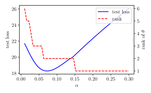
Figure 1: Test loss and rank of $\theta$ versus $\alpha$ on the simulated dataset.

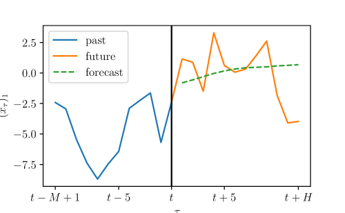
Figure 2: Forecast of simulated data made at a time $t$, shown as vertical line. The solid curve shows $(x_{\tau})_{1}$, and the dashed line is our forecast, $(\hat{x}_{\tau\mid t})_{1}$, $\tau=t+1,\ldots,t+H$.

We can also compare our extracted latent state to the true latent state. As mentioned above, the latent state is modulo a linear change of coordinates, so to compare the true latent state and the latent state of our forecaster, we use our latent state to predict the true latent state of the underlying state space model, by choosing $S$ to minimize

$$\sum_{t=M}^{T-H}\|SU^{T}p_{t}-z_{t}\|_{2}^{2}$$

over the coordinate transformation $S\in{\mbox{\bf R}}^{2\times 2}$. In figure 3 we plot the transformed states. We can see that our transformed latent states reasonably track the true latent states.

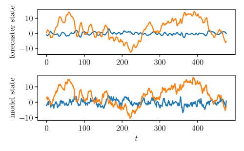
Figure 3: Simulated dataset. Top. Transformed latent state of the forecaster. Bottom. True latent state of underlying state space model.

We can trade off forecaster consistency for performance. We fit the forecaster with $\alpha=0.1$ for a number of values of $\kappa\in[10^{-2},10^{1}]$. In figure 4 we compare the train and test loss versus the train and test forecaster consistency for these values of $\kappa$. To improve forecaster consistency, we have to sacrifice performance (e.g., a 1000x reduction in forecaster consistency more than doubles our test loss). Finally, in figure 5 we demonstrate the effect of encouraging forecaster consistency.

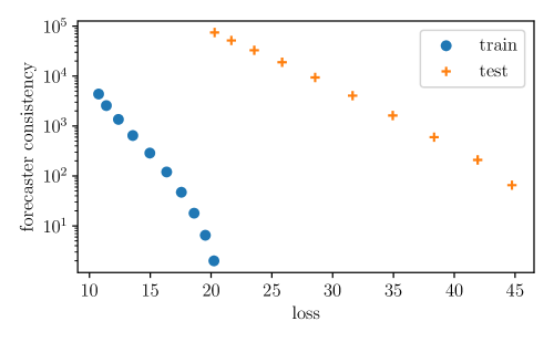
Figure 4: Simulated dataset. Loss versus forecaster consistency on the train and test dataset for a number of $\kappa$s.

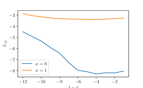
Figure 5: Simulated dataset. Forecasts of $(x_{\tau})_{1}$ made at $t=\tau-1,\ldots,\tau-H$ for two forecasters: one with $\kappa=0$ and one with $\kappa=1$. Notice that the forecasts are much more consistent and barely change when $\kappa=1$.

6.2 Stock index absolute returns

In this example, we use previous absolute returns of a stock index to forecast future absolute returns of the index. It has been observed that stocks exhibit volatility clustering, first observed by Mandelbrot when he wrote “large changes tend to be followed by large changes, of either sign, and small changes tend to be followed by small changes” [32]. In this example we use the techniques of low rank forecasting to analyze volatility clustering. Along the way, we find that the latent state in a rank one forecaster very closely resembles the CBOE Volatility index (VIX), an index that tracks the 30-day expected volatility of the US stock market. We note that our model is very similar in spirit to a GARCH model, which has been observed to work well for modeling market volatility [33].

We gathered the daily absolute return of the SPY ETF (exchange traded fund), an ETF that closely tracks the S&P 500 index, from February 1993 to October 2020 ($T\approx 7000$). We annualize the daily absolute return by multiplying them by $\sqrt{250}$. We split the original dataset in half, into a training and test dataset. We also pre-process both datasets by subtracting the mean of $\{x_{t}\}$ on the training dataset from both the training and test dataset.

Our goal will be to predict the next month of SPY’s absolute returns ($H=20$ trading days) from the past quarter of SPY’s absolute returns ($M=60$ trading days). The parameter $\theta$ is thus a 60 by 20 matrix, containing $1200$ entries.

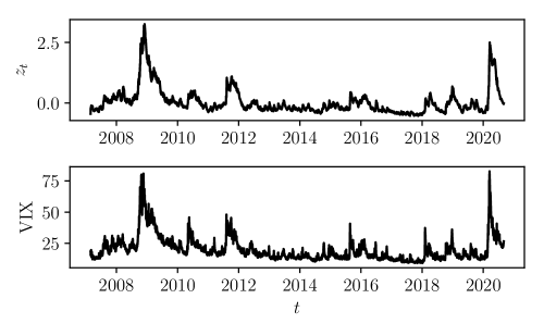
Figure 6: Top. Latent state in rank one forecaster on (unseen) test set. Bottom. VIX index.

We tried a number of values of $\alpha$, and found that $\alpha=0.05$ worked well, and corresponds to a rank one forecaster. Fitting each forecaster took roughly four seconds, not using warm-start. (Warm starting the optimization from the previous value of $\alpha$ reduced this considerably.) The test loss of this forecaster is 0.022; for comparison, the test loss for the mean forecaster is 0.026, meaning our forecaster provides a 15% percent improvement in test loss. In figure 7 we show a forecast from our model on the test dataset. In figure 8 we show the forecaster test loss versus horizon (how many steps it is forecasting out). As expected, the test loss increases as we forecast further out.

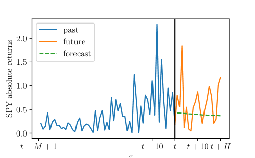
Figure 7: SPY absolute return forecast.

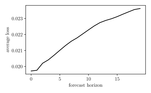
Figure 8: Test loss at different forecast horizons in forecasting SPY absolute returns.

In figure 6 we plot the latent state of the forecaster, along with the VIX, on the test set. At least visually, the forecaster’s latent state looks like a (shifted and scaled) smooth version of the VIX. To investigate the correlation between the forecaster latent state and VIX, we took the deciles of both series, and calculated the number of times each series were in their respective deciles. In figure 9 we show a heatmap of the deciles. When the VIX index is in its highest decile, the forecaster latent state is also in its highest decile over 80% of the time. The heatmap looks very close to diagonal, so we can conclude that the two time series are very correlated.

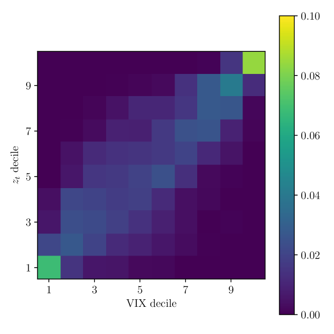
Figure 9: Heatmap of $z_{t}$ and VIX deciles.

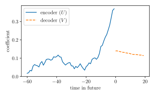
Figure 10: SPY forecaster factors. We filter the last 60 days of absolute returns using $U$ to get a single latent state, and then multiply the latent state by $V$ to get our forecast.

Since the encoder $U$ and the decoder $V$ are both vectors (indeed one-dimensional filters), we can plot them. In figure 10 we show the parameters of the encoder and decoder. We can see that the decoder is most sensitive to the most recent values of the series, and also assigns high importance to the absolute returns 40 trading days ago (around $i=20$). We also observe that the decoder $V$ is roughly decreasing in $i$; this means that the farther out we are forecasting, the closer the forecast gets to 0, or to simply predicting the mean value.

6.3 Traffic

We consider a dataset from the Caltrans performance measurement system (PeMS), which is composed of hourly road occupancy rates at $n=100$ stations located on highways in Caltrans District 4 (the San Francisco Bay Area) from October 2019 to December 2019 [34] ($T=2000$). Each data entry is the average occupancy rate over the hour, between 0 and 1, which is roughly the average fraction of the time each vehicle was present in that segment over 30 second windows (for more details see [34]).

Pre-processing.

We carried out several pre-processing steps. We first clip or Winsorize the raw occupancy rates $o_{t}$ to be in $[0.001,0.999]$, and then perform a logit transform, i.e.,

$$\log\left(\frac{o_{t}}{1-o_{t}}\right),$$

where division and $\log$ are elementwise. (This yields a more normal distribution.)

We split the dataset in half into a training and test dataset. We subtracted the mean occupancy rate on the training dataset for each station from the occupancy rates in both the training and test dataset. We take $M=24$ and $H=6$, so from the last day of traffic we predict the next quarter day of traffic. In total, there are around 1.4 million parameters in a linear forecaster. We use the $\ell_{2}$ (squared) loss. The loss of the constant (mean) forecaster was 1.108 on the training dataset and 0.962 on the test dataset.

De-trending.

We de-trend the time series as described in §5.3 by using auxiliary time-based features. As auxiliary features we use sine and cosine of hour (with periods of 24, 12, 8, 6, and 24/5 hours), hour in week (at harmonic periods of 168, 168/2, 168/3, 168/4, and 168/5 hours), and a binary weekday/weekend feature. We also use all pairwise products of these auxiliary features, which for products of sines and cosines are sinusoids at the sum and difference frequencies. In total there are 462 auxiliary features. This (deterministic) baseline model yields a training loss of 0.099 and a test loss of 0.203.

Forecasting.

Next, we construct a low rank forecaster for the residual series. Figure 11 shows the rank and test loss versus the regularization parameter $\alpha$. The choice $\alpha=0.07$ yields a rank 14 forecaster with a test loss of 0.184, and improvement of around 10% over the baseline model. Fitting the forecaster takes around 11 seconds. An example forecast is shown in figure 12.

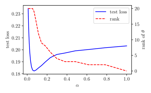
Figure 11: Test loss and rank of $\theta$ versus $\alpha$ on the traffic dataset.

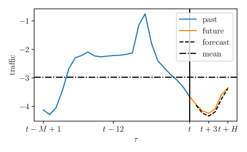
Figure 12: Forecast of traffic data made at a time $t$, shown as vertical line. The solid curve shows $(x_{\tau})_{1}$, and the dashed line is our forecast of the logit occupancy, $(\hat{x}_{\tau\mid t})_{1}$, $\tau=t+1,\ldots,t+H$.

7 Related work

The general problem of time series forecasting has been studied for decades, and many books have been written on the subject [35, 36, 37, 5, 38, 39, 40]. Many methods have been developed, and we survey a subset of them below. We try to focus on methods that are by our definition low rank, i.e., the forecast can be decomposed as first computing a lower dimensional vector (the latent state) from the past, and then computing the forecast based on that low dimensional vector. We also survey general work on general statistical modeling of time series and low rank decompositions.

Classical time series models.

Classical models of time series model them as stationary stochastic processes. Given the random process, the optimal (in terms of mean squared loss) forecaster is the conditional mean forecaster, i.e., the forecast of future values is the mean of the future values given the observed past [5, §5]. Some common linear models that fall under this category are the Wiener filter [41], exponential smoothing [42, 43], moving average [5, §3.3], autoregressive [5, §3.2], ARMA [5, §3.4], and ARIMA [5, §4]. Most of these models are Markov processes, meaning the future is independent of the past, given a particular state or summarization of the past [44]. Most of these models are also special cases of linear state space models [1], and exact forecasting can be done by first Kalman filtering, and then iterating the state space model without disturbances [5, §5.5]. There exist many methods to fit state space models to data [5, §7], including N4SID [12], EM [13, 45], and least squares auto-tuning [14]. State space models are very closely related to dynamic factor models [46, 47, 48, 49, 50, 51, 52], which have found applications in economics [53, 54, 55, 56, 57, 58, 59, 60, 61]. Our paper is focused on the problem of forecasting, and does not explicitly construct a stochastic model of the time series.

Minimum order system identification.

A closely related problem in system identification is finding the minimal order representation of a linear system [9, 10]. One approach is to construct a Hankel matrix of impulse responses, which was first proposed by Ho and Kalman [62], and later expanded upon by Tether [63], Risannen [64], Woodside [65], Silverman [66], Akaike [67], Chow [68, 69], and Aoki [70, 71]. These early papers spawned the field of subspace identification [72, 73], which has resulted in techniques like N4SID [74, 75, 76, 12], which take the SVD of a particular block Hankel matrix, and related techniques like MOESP [77, 78, 79] and CVA [80, 81] (see, e.g., [82, §10.6] for a summary). We also point the reader to the paper by Jansson [83], which poses subspace identification methods as a regression, where the forecasting matrix is low rank.

Low rank matrix approximation.

The techniques in this paper are closely related to the formation of low rank approximations to matrices, which dates all the way back to Eckart’s seminal work on principal component analysis (PCA) [84]. The basis of PCA is that the truncated SVD of a matrix is the best low rank approximation of the matrix (in terms of Frobenius norm), and has been expanded heavily and generalized to different data types, objective functions, and regularization functions [85, 27]. A standard convex, continuous approximation of the rank function is the nuclear norm function [86], and convex optimization problems involving nuclear norms can be expressed as semidefinite programs [87], and efficient solution methods exist (see, e.g., [88, 89]). The nuclear norm also exhibits a number of nice theoretical properties, e.g., it can be used to recover the true minimum rank solution for certain problems [90], and near-optimal solutions in others [91]. It has also proved to be a useful heuristic for system identification problems [86, 92, 93, 94]. For more discussion on the nuclear norm, and its applications, see, e.g., [95, 96, 97, 98, 99, 100] and the references therein.

Reduced rank prediction.

A closely related problem is reduced rank prediction. Reduced rank regression can be traced back to the work [101], where a likelihood-ratio test is obtained for the hypothesis that the rank of the regression coefficient matrix is a given number. Later, the work [102] provided an explicit form of the estimate of the regression coefficient matrix with a given rank, and discussed the asymptotics of the estimated regression coefficient matrix. The reduced rank regression problem was approximately solved as a nuclear norm penalized least squares problem in [103], and then further generalized into an adaptive nuclear norm penalized reduced rank regression problem in [104]. For more details on reduced rank regression, please refer to [105]. The optimization problem in the form of a loss function plus a nuclear norm regularization term has applications in in multi-task learning; see, e.g., [106, 107, 108, 95].

Reduced rank time series.

Similar to reduced rank regression, reduced rank time series modeling is also closely connected with the low rank forecasting problem. Early work such as [109, 110, 111] fit reduced rank coefficient models to vector time series to provide a concise representation of vector time series models. Many of these models work by extracting a lower dimensional vector time series from the past first, and then perform one-step ahead forecast (which corresponds to $H=1$) based on the extracted low dimensional vector time series. This is very similar to the (low rank) two step forecasting technique discussed in this paper. The reduced rank modeling problem has been generalized into the structured VAR modeling problem [112, 113, 114]. In these papers, regularization terms are added to encourage certain structures. For example, a nuclear norm term is often used to encourage the transition matrix to be low rank, and $\ell_{1}$ norm is used to encourage the transition matrix to be sparse.

Extracting a low-dimensional predictable time series.

Another related problem is extract a low-dimensional (self-)predictable time series from a high-dimensional vector time series. The paper [115] is an early one with the explicit goal of predictability. After this, many other methods have been developed in different research areas on extracting predictable time series, including economics [115, 116, 117, 118, 119], machine learning [120, 121, 122], process system engineering [123, 124, 125, 126], signal processing, and atmospheric research [127, 128, 129]. Another closely related line of work is on predictive state representations [130, 131, 132].

Nonlinear forecasters.

There also exist many nonlinear forecasting methods. These methods are often based on neural networks, e.g., recurrent neural networks [133, 134, 135, 136, 137, 138], convolutional neural networks [139, 140, 141], and autoencoders [142, 143, 144]. Other nonlinear forecasting methods include regime switching models [145, 146] and NARMAX models [147, 148]. Recently, there have also been methods proposed that perform vector time series forecasting through matrix completion, where the vector time series are assumed share some common structures [149, 150].

Appendix A Gradients

Loss plus nuclear norm.

Let

$$\mathcal{L}(U,V)=\frac{1}{N}\mathbf{1}^{T}\ell(PUV-F)+\frac{\lambda}{2}(\|U\|_{F}^{2}+\|V\|_{F}^{2})$$

denote the loss plus nuclear norm part of the objective in problem (5). Let

$$g_{i}=\nabla_{\hat{f}_{i}}\ell(\hat{f}_{i})\in{\mbox{\bf R}}^{Hn},\quad i=1,\ldots,N$$

denote the gradient of the loss with respect to the forecast of the $i$th data point. We have that

$$\nabla_{U}\mathcal{L}(U,V)=\frac{1}{N}\sum_{i=1}^{N}p_{i}g_{i}^{T}V^{T}+\lambda U,\qquad\nabla_{V}\mathcal{L}(U,V)=\frac{1}{N}\sum_{i=1}^{N}U^{T}p_{i}g_{i}^{T}+\lambda V.$$

Forecaster consistency.

To compute the gradient of the forecaster consistency loss with respect to $U$ and $V$, we first compute the gradient with respect to $\theta$, denoted

$$G=\nabla\mathcal{I}_{\theta}(\theta)=P^{T}(\nabla_{\hat{F}}\mathop{\bf dist{}}(\hat{F})^{2}).$$

The matrix $\nabla_{\hat{F}}\mathop{\bf dist{}}(\hat{F})^{2}$ is the gradient of the forecaster consistency with respect to the forecasts $\hat{F}$, and its (block) elements are given by

$$g_{\tau\mid t}=\nabla_{x_{\tau\mid t}}\mathop{\bf dist{}}(\hat{F})^{2}=2(\hat{x}_{\tau\mid t}-\bar{x}_{\tau})-\sum_{t_{1}=\max\{\tau-H,M+1\}}^{\min\{\tau-1,T-H\}}\frac{2}{f(\tau)}(\hat{x}_{\tau\mid t_{1}}-\bar{x}_{\tau}),$$

where

$$f(\tau)=\min\{\tau,T-H+1\}-\max\{\tau-H,M+1\},\quad\tau=M+1,\ldots,T.$$

Then, using $G$, the gradients of forecaster consistency with respect to $U$ and $V$ are

$$\nabla_{U}\mathcal{I}(UV)=GV^{T},\qquad\nabla_{V}\mathcal{I}(UV)=U^{T}G.$$

References

- [1] Rudolf Kalman. A new approach to linear filtering and prediction problems. Journal Basic Engineering, 82(1):35–45, 1960.
- [2] Stephen Boyd and Lieven Vandenberghe. Convex optimization. Cambridge University Press, 2004.
- [3] Gilles Hilary and Charles Hsu. Analyst forecast consistency. Journal of Finance, 68(1):271–297, 2013.
- [4] John Gubner. Probability and random processes for electrical and computer engineers. Cambridge University Press, 2006.
- [5] George Box, Gwilym Jenkins, and Gregory Reinsel. Time series analysis: forecasting and control. Wiley, 2008.
- [6] Trevor Hastie, Robert Tibshirani, and Jerome Friedman. The elements of statistical learning: data mining, inference, and prediction. Springer Science & Business Media, 2009.
- [7] Mohsen Pourahmadi. High-dimensional covariance estimation: with high-dimensional data. John Wiley & Sons, 2013.
- [8] John Burg. A new analysis technique for time series data. NATO Advanced Study Institute on Signal Processing, 1968.
- [9] Elmer Gilbert. Controllability and observability in multivariable control systems. Journal of the Society for Industrial and Applied Mathematics, Series A: Control, 1(2):128–151, 1963.
- [10] Rudolf Kalman. Mathematical description of linear dynamical systems. Journal of the Society for Industrial and Applied Mathematics, Series A: Control, 1(2):152–192, 1963.
- [11] Masanao Aoki. State space modeling of time series. Springer Science & Business Media, 2013.
- [12] Peter Van Overschee and Bart De Moor. N4SID: Subspace algorithms for the identification of combined deterministic-stochastic systems. Automatica, 30(1):75–93, 1994.
- [13] Robert Shumway and David Stoffer. An approach to time series smoothing and forecasting using the EM algorithm. Journal Time Series Analysis, 3(4):253–264, 1982.
- [14] Shane Barratt and Stephen Boyd. Fitting a Kalman smoother to data. In American Control Conference (ACC), pages 1526–1531. IEEE, 2020.
- [15] Stephen Boyd and Lieven Vandenberghe. Introduction to applied linear algebra: vectors, matrices, and least squares. Cambridge University Press, June 2018.
- [16] Steven Diamond and Stephen Boyd. CVXPY: A Python-embedded modeling language for convex optimization. Journal of Machine Learning Research, 17(83):1–5, 2016.
- [17] Akshay Agrawal, Robin Verschueren, Steven Diamond, and Stephen Boyd. A rewriting system for convex optimization problems. Journal of Control and Decision, 5(1):42–60, 2018.
- [18] Shuiwang Ji and Jieping Ye. An accelerated gradient method for trace norm minimization. In Proc. Intl. Conf. Machine Learning, pages 457–464, 2009.
- [19] Yuanyuan Liu, Hong Cheng, Fanhua Shang, and James Cheng. Nuclear norm regularized least squares optimization on Grassmannian manifolds. In Proc. Uncertainty in Artificial Intelligence, pages 515–524. AUAI Press, 2014.
- [20] Kim-Chuan Toh and Sangwoon Yun. An accelerated proximal gradient algorithm for nuclear norm regularized linear least squares problems. Pacific Journal of Optimization, 6(615-640):15, 2010.
- [21] Raghunandan Keshavan. Efficient algorithms for collaborative filtering. PhD thesis, Stanford University, 2012.
- [22] Caihua Chen, Bingsheng He, and Xiaoming Yuan. Matrix completion via an alternating direction method. IMA Journal of Numerical Analysis, 32(1):227–245, 2012.
- [23] Prateek Jain, Praneeth Netrapalli, and Sujay Sanghavi. Low-rank matrix completion using alternating minimization. In Proc. ACM Symposium on Theory of Computing, pages 665–674, 2013.
- [24] Moritz Hardt. On the provable convergence of alternating minimization for matrix completion. arXiv preprint arXiv:1312.0925, 2013.
- [25] Praneeth Netrapalli, UN Niranjan, Sujay Sanghavi, Animashree Anandkumar, and Prateek Jain. Non-convex robust pca. In Advances in Neural Information Processing Systems, pages 1107–1115, 2014.
- [26] Alekh Agarwal, Animashree Anandkumar, Prateek Jain, and Praneeth Netrapalli. Learning sparsely used overcomplete dictionaries via alternating minimization. SIAM Journal on Optimization, 26(4):2775–2799, 2016.
- [27] Madeleine Udell, Corinne Horn, Reza Zadeh, and Stephen Boyd. Generalized low rank models. Foundations and Trends® in Machine Learning, 9(1):1–118, 2016.
- [28] Dong Liu and Jorge Nocedal. On the limited memory BFGS method for large scale optimization. Mathematical Programming, 45(1-3):503–528, 1989.
- [29] Ian Goodfellow, Yoshua Bengio, and Aaron Courville. Deep learning. MIT Press, 2016.
- [30] Nicholas Moehle, Enzo Busseti, Stephen Boyd, and Matt Wytock. Dynamic energy management. In Large Scale Optimization in Supply Chains and Smart Manufacturing, volume 149, pages 69–126. Springer International Publishing, 2019.
- [31] Adam Paszke, Sam Gross, Francisco Massa, Adam Lerer, James Bradbury, Gregory Chanan, Trevor Killeen, Zeming Lin, Natalia Gimelshein, Luca Antiga, and others. PyTorch: An imperative style, high-performance deep learning library. In Advances in Neural Information Processing Systems, pages 8024–8035, 2019.
- [32] Benoit Mandelbrot. The variation of certain speculative prices. The Journal of Business, 36(4):394–419, 1963.
- [33] Zhuanxin Ding and Clive W. J. Granger. Modeling volatility persistence of speculative returns: A new approach. Journal of Econometrics, 73(1):185–215, July 1996.
- [34] Tom Choe, Alexander Skabardonis, and Pravin Varaiya. Freeway performance measurement system (PeMS): An operational analysis tool. 81st Annual Meeting, Transportation Research Board, 2001.
- [35] Chris Chatfield. Time-series forecasting. CRC press, 2000.
- [36] Helmut Lütkepohl. New introduction to multiple time series analysis. Springer Science & Business Media, 2005.
- [37] Jan De Gooijer and Rob Hyndman. 25 years of time series forecasting. International Journal of Forecasting, 22(3):443–473, 2006.
- [38] Peter Brockwell, Richard Davis, and Matthew Calder. Introduction to time series and forecasting, volume 2. Springer, 2002.
- [39] John Granger and Paul Newbold. Forecasting economic time series. Academic Press, 2014.
- [40] James Hamilton. Time series analysis. Princeton University Press, 2020.
- [41] Norbert Wiener. Extrapolation, interpolation, and smoothing of stationary time series: with engineering applications. MIT Press, 1950.
- [42] Robert Brown. Exponential smoothing for predicting demand. In Operations Research, volume 5, pages 145–145, 1957.
- [43] Charles Holt. Forecasting trends and seasonal by exponentially weighted moving averages. ONR Memorandum, 52, 1957.
- [44] Andrei Markov. The theory of algorithms. Trudy Matematicheskogo Instituta Imeni VA Steklova, 42:3–375, 1954.
- [45] Elizabeth Holmes. Derivation of the EM algorithm for constrained and unconstrained MARSS models. 2012.
- [46] Ben Bernanke, Jean Boivin, and Piotr Eliasz. Measuring the effects of monetary policy: a factor-augmented vector autoregressive (FAVAR) approach. The Quarterly Journal of Economics, 120(1):387–422, 2005.
- [47] Mario Forni, Marc Hallin, Marco Lippi, and Lucrezia Reichlin. The generalized dynamic factor model: one-sided estimation and forecasting. Journal of the American Statistical Association, 100(471):830–840, 2005.
- [48] James Stock and Mark Watson. Forecasting with many predictors. Handbook of Economic Forecasting, 1:515–554, 2006.
- [49] Jushan Bai and Serena Ng. Determining the number of primitive shocks in factor models. Journal of Business & Economic Statistics, 25(1):52–60, 2007.
- [50] James Stock and Mark Watson. Dynamic factor models. Oxford Handbooks Online, 2011.
- [51] In Choi. Efficient estimation of factor models. Econometric Theory, pages 274–308, 2012.
- [52] Daniel Peña, Ezequiel Smucler, and Victor Yohai. Forecasting multiple time series with one-sided dynamic principal components. Journal of the American Statistical Association, 114(528):1683–1694, 2019.
- [53] John Geweke. The dynamic factor analysis of economic time series. Latent variables in socio-economic models, 1977.
- [54] Stephen Figlewski. Optimal price forecasting using survey data. The Review of Economics and Statistics, pages 13–21, 1983.
- [55] Stephen Figlewski and Thomas Urich. Optimal aggregation of money supply forecasts: Accuracy, profitability and market efficiency. The Journal of Finance, 38(3):695–710, 1983.
- [56] Danny Quah and Thomas Sargent. A dynamic index model for large cross sections. In Business Cycles, Indicators, and Forecasting, pages 285–310. University of Chicago Press, 1993.
- [57] James Stock and Mark Watson. Forecasting inflation. Journal of Monetary Economics, 44(2):293–335, 1999.
- [58] James Stock and Mark Watson. Forecasting using principal components from a large number of predictors. Journal of the American Statistical Association, 97(460):1167–1179, 2002.
- [59] Ben Bernanke and Jean Boivin. Monetary policy in a data-rich environment. Journal of Monetary Economics, 50(3):525–546, 2003.
- [60] Theodore Crone and Alan Clayton-Matthews. Consistent economic indexes for the 50 states. Review of Economics and Statistics, 87(4):593–603, 2005.
- [61] Jean Boivin and Serena Ng. Are more data always better for factor analysis? Journal of Econometrics, 132(1):169–194, 2006.
- [62] Bin-Lun Ho and Rudolf Kalman. Effective construction of linear state-variable models from input/output functions. at-Automatisierungstechnik, 14(1-12):545–548, 1966.
- [63] Anthony Tether. Construction of minimal linear state-variable models from finite input-output data. IEEE Transactions on Automatic Control, 15(4):427–436, 1970.
- [64] Jorma Rissanen. Recursive identification of linear systems. SIAM Journal on Control, 9(3):420–430, 1971.
- [65] CM Woodside. Estimation of the order of linear systems. Automatica, 7(6):727–733, 1971.
- [66] Leonard Silverman. Realization of linear dynamical systems. IEEE Transactions on Automatic Control, 16(6):554–567, 1971.
- [67] Hirotugu Akaike. Stochastic theory of minimal realization. IEEE Transactions on Automatic Control, 19(6):667–674, 1974.
- [68] Joseph Chow. On estimating the orders of an autoregressive moving-average process with uncertain observations. IEEE Transactions on Automatic Control, 17(5):707–709, 1972.
- [69] Joseph Chow. On the estimation of the order of a moving-average process. IEEE Transactions on Automatic Control, 17(3):386–387, 1972.
- [70] Masanao Aoki. Estimation of system matrices: Initial phase. In Notes on Economic Time Series Analysis: System Theoretic Perspectives, pages 60–89. Springer, 1983.
- [71] Masanao Aoki. Prediction of time series. In Notes on Economic Time Series Analysis: System Theoretic Perspectives, pages 38–47. Springer, 1983.
- [72] Tohru Katayama. Subspace methods for system identification. Springer Science & Business Media, 2006.
- [73] Peter Van Overschee and Bart De Moor. Subspace identification for linear systems: Theory-Implementation-Applications. Springer Science & Business Media, 2012.
- [74] Marc Moonen, Bart De Moor, Lieven Vandenberghe, and Joos Vandewalle. On-and off-line identification of linear state-space models. International Journal of Control, 49(1):219–232, 1989.
- [75] Peter Van Overschee and Bart De Moor. Two subspace algorithms for the identification of combined deterministic-stochastic systems. In Proc. Conference on Decision and Control, pages 511–516. IEEE, 1992.
- [76] Peter Van Overschee and Bart De Moor. Subspace algorithms for the stochastic identification problem. Automatica, 29(3):649–660, 1993.
- [77] Michel Verhaegen. A novel non-iterative MIMO state space model identification technique. IFAC Proceedings Volumes, 24(3):749–754, 1991.
- [78] Michel Verhaegen and Patrick Dewilde. Subspace model identification part 2. Analysis of the elementary output-error state-space model identification algorithm. International Journal of Control, 56(5):1211–1241, 1992.
- [79] Michel Verhaegen. Subspace model identification part 3. Analysis of the ordinary output-error state-space model identification algorithm. International Journal of Control, 58(3):555–586, 1993.
- [80] Wallace Larimore. System identification, reduced-order filtering and modeling via canonical variate analysis. In Proc. American Control Conference, pages 445–451. IEEE, 1983.
- [81] Wallace Larimore. Canonical variate analysis in identification, filtering, and adaptive control. In Proc. Conf. Decision and Control, pages 596–604. IEEE, 1990.
- [82] Lennart Ljung. System identification. Wiley Encyclopedia of Electrical and Electronics Engineering, pages 1–19, 1999.
- [83] Magnus Jansson and Bo Wahlberg. A linear regression approach to state-space subspace system identification. Signal Processing, 52(2):103–129, 1996.
- [84] Carl Eckart and Gale Young. The approximation of one matrix by another of lower rank. Psychometrika, 1(3):211–218, 1936.
- [85] Moody Chu, Robert Funderlic, and Robert Plemmons. Structured low rank approximation. Linear Algebra and Its Applications, 366:157–172, 2003.
- [86] Maryam Fazel, Haitham Hindi, and Stephen Boyd. A rank minimization heuristic with application to minimum order system approximation. In Proc. American Control Conference, volume 6, pages 4734–4739. IEEE, 2001.
- [87] Lieven Vandenberghe and Stephen Boyd. Semidefinite programming. SIAM Review, 38(1):49–95, 1996.
- [88] Zhang Liu and Lieven Vandenberghe. Interior-point method for nuclear norm approximation with application to system identification. SIAM Journal on Matrix Analysis and Applications, 31(3):1235–1256, 2010.
- [89] Jian-Feng Cai, Emmanuel Candès, and Zuowei Shen. A singular value thresholding algorithm for matrix completion. SIAM Journal on Optimization, 20(4):1956–1982, 2010.
- [90] Benjamin Recht, Maryam Fazel, and Pablo Parrilo. Guaranteed minimum-rank solutions of linear matrix equations via nuclear norm minimization. SIAM review, 52(3):471–501, 2010.
- [91] Emmanuel Candès and Terence Tao. The power of convex relaxation: near-optimal matrix completion. IEEE Transactions on Information Theory, 56(5):2053–2080, 2010.
- [92] Karthik Mohan and Maryam Fazel. Reweighted nuclear norm minimization with application to system identification. In Proc. American Control Conference, pages 2953–2959. IEEE, 2010.
- [93] Anders Hansson, Zhang Liu, and Lieven Vandenberghe. Subspace system identification via weighted nuclear norm optimization. In Proc. IEEE Conf. Decision and Control, pages 3439–3444, 2012.
- [94] Maryam Fazel, Ting Kei Pong, Defeng Sun, and Paul Tseng. Hankel matrix rank minimization with applications to system identification and realization. SIAM Journal on Matrix Analysis and Applications, 34(3):946–977, 2013.
- [95] Ting Pong, Paul Tseng, Shuiwang Ji, and Jieping Ye. Trace norm regularization: reformulations, algorithms, and multi-task learning. SIAM Journal on Optimization, 20(6):3465–3489, 2010.
- [96] Sahand Negahban and Martin Wainwright. Estimation of (near) low-rank matrices with noise and high-dimensional scaling. Annals of Statistics, 39(2):1069–1097, 2011.
- [97] Shiqian Ma, Donald Goldfarb, and Lifeng Chen. Fixed point and Bregman iterative methods for matrix rank minimization. Mathematical Programming, 128(1-2):321–353, June 2011.
- [98] Ivan Markovsky and Konstantin Usevich. Low rank approximation, volume 139. Springer, 2012.
- [99] Ivan Markovsky. How effective is the nuclear norm heuristic in solving data approximation problems? IFAC Proceedings Volumes, 45(16):316–321, 2012.
- [100] Ohad Shamir and Shai Shalev-Shwartz. Matrix completion with the trace norm: learning, bounding, and transducing. The Journal of Machine Learning Research, 15(1):3401–3423, 2014.
- [101] Theodore Anderson. Estimating linear restrictions on regression coefficients for multivariate normal distributions. The Annals of Mathematical Statistics, 22(3):327–351, 1951.
- [102] Alan Izenman. Reduced-rank regression for the multivariate linear model. Journal of Multivariate Analysis, 5(2):248–264, 1975.
- [103] Ming Yuan, Ali Ekici, Zhaosong Lu, and Renato Monteiro. Dimension reduction and coefficient estimation in multivariate linear regression. Journal of the Royal Statistical Society: Series B (Statistical Methodology), 69(3):329–346, 2007.
- [104] Kun Chen, Hongbo Dong, and Kung-Sik Chan. Reduced rank regression via adaptive nuclear norm penalization. Biometrika, 100(4):901–920, 2013.
- [105] Raja Velu and Gregory Reinsel. Multivariate reduced-rank regression: theory and applications, volume 136. Springer Science & Business Media, 2013.
- [106] Rich Caruana. Multitask learning. In Learning to Learn, pages 95–133. Boston, MA, 1998.
- [107] Yonatan Amit, Michael Fink, Nathan Srebro, and Shimon Ullman. Uncovering shared structures in multiclass classification. In Proc. Intl. Conf. Machine Learning, pages 17–24, June 2007.
- [108] Andreas Argyriou, Theodoros Evgeniou, and Massimiliano Pontil. Convex multi-task feature learning. Machine Learning, 73(3):243–272, 2008.
- [109] Sung Ahn and Gregory Reinsel. Nested reduced-rank autoregressive models for multiple time series. Journal of the American Statistical Association, 83(403):849–856, 1988.
- [110] Raja Velu, Gregory Reinsel, and Dean Wichern. Reduced rank models for multiple time series. Biometrika, 73(1):105–118, 1986.
- [111] Zijun Wang and David Bessler. Forecasting performance of multivariate time series models with full and reduced rank: an empirical examination. International Journal of Forecasting, 20(4):683–695, 2004.
- [112] Sumanta Basu, Xianqi Li, and George Michailidis. Low rank and structured modeling of high-dimensional vector autoregressions. IEEE Transactions on Signal Processing, 67(5):1207–1222, 2019.
- [113] Pierre Alquier, Karine Bertin, Paul Doukhan, and Rémy Garnier. High-dimensional VAR with low-rank transition. Statistics and Computing, 30(4):1139–1153, 2020.
- [114] Igor Melnyk and Arindam Banerjee. Estimating structured vector autoregressive models. In Proc. Intl. Conf. Machine Learning, pages 830–839, 2016.
- [115] George Box and George Tiao. A canonical analysis of multiple time series. Biometrika, 64(2):355–365, 1977.
- [116] Daniel Pena and George Box. Identifying a simplifying structure in time series. Journal of the American Statistical Association, 82(399):836–843, 1987.
- [117] Clifford Lam, Qiwei Yao, and Neil Bathia. Estimation of latent factors for high-dimensional time series. Biometrika, 98(4):901–918, 2011.
- [118] Clifford Lam and Qiwei Yao. Factor modeling for high-dimensional time series: inference for the number of factors. The Annals of Statistics, 40(2):694–726, 2012.
- [119] Yining Dong, Joe Qin, and Stephen Boyd. Extracting a low-dimensional predictable time series. 2019.
- [120] James Stone. Blind source separation using temporal predictability. Neural Computation, 13(7):1559–1574, 2001.
- [121] Stefan Richthofer and Laurenz Wiskott. Predictable feature analysis. In Proc. IEEE Intl. Conf. Machine Learning and Applications, pages 190–196. IEEE, 2015.
- [122] Georg Goerg. Forecastable component analysis. In Intl. Conf. Machine Learning, pages 64–72, 2013.
- [123] Gang Li, Joe Qin, and Donghua Zhou. A new method of dynamic latent-variable modeling for process monitoring. IEEE Transactions on Industrial Electronics, 61(11):6438–6445, 2014.
- [124] Le Zhou, Gang Li, Zhihuan Song, and Joe Qin. Autoregressive dynamic latent variable models for process monitoring. IEEE Transactions on Control Systems Technology, 25(1):366–373, 2016.
- [125] Yining Dong and Joe Qin. Dynamic latent variable analytics for process operations and control. Computers & Chemical Engineering, 114:69–80, 2018.
- [126] Yining Dong and Joe Qin. A novel dynamic PCA algorithm for dynamic data modeling and process monitoring. Journal of Process Control, 67:1–11, 2018.
- [127] Timothy DelSole. Optimally persistent patterns in time-varying fields. Journal of the Atmospheric Sciences, 58(11):1341–1356, 2001.
- [128] Timothy DelSole and Michael Tippett. Average predictability time. Part I: theory. Journal of the Atmospheric Sciences, 66(5):1172–1187, 2009.
- [129] Timothy DelSole and Michael Tippett. Average predictability time. Part II: Seamless diagnoses of predictability on multiple time scales. Journal of the Atmospheric Sciences, 66(5):1188–1204, 2009.
- [130] Michael Littman, Richard Sutton, and Satinder Singh. Predictive representations of state. Proc. Adv. Neural Inf. Process. Syst., 14, 2002.
- [131] Matthew Rosencrantz, Geoff Gordon, and Sebastian Thrun. Learning low dimensional predictive representations. In Proc. Intl. Conf. Machine Learning, page 88, 2004.
- [132] Byron Boots, Sajid Siddiqi, and Geoffrey Gordon. Closing the learning-planning loop with predictive state representations. The International Journal of Robotics Research, 30(7):954–966, 2011.
- [133] Jerome Connor, Douglas Martin, and Les Atlas. Recurrent neural networks and robust time series prediction. IEEE Transactions on Neural Networks, 5(2):240–254, 1994.
- [134] Zhengping Che, Sanjay Purushotham, Kyunghyun Cho, David Sontag, and Yan Liu. Recurrent neural networks for multivariate time series with missing values. Scientific Reports, 8(1):1–12, 2018.
- [135] Matteo Maggiolo and Gerasimos Spanakis. Autoregressive convolutional recurrent neural network for univariate and multivariate time series prediction. arXiv preprint arXiv:1903.02540, 2019.
- [136] Sima Siami-Namini and Akbar Namin. Forecasting economics and financial time series: ARIMA vs. LSTM. arXiv preprint arXiv:1803.06386, 2018.
- [137] Felix Gers, Douglas Eck, and Jürgen Schmidhuber. Applying LSTM to time series predictable through time-window approaches. In Neural Nets WIRN, pages 193–200. Springer, 2002.
- [138] Kai Chen, Yi Zhou, and Fangyan Dai. A LSTM-based method for stock returns prediction: A case study of China stock market. In Proc. IEEE Intl. Conf. Big Data, pages 2823–2824. IEEE, 2015.
- [139] Ioannis Livieris, Emmanuel Pintelas, and Panagiotis Pintelas. A CNN–LSTM model for gold price time-series forecasting. Neural Computing and Applications, pages 1–10, 2020.
- [140] Mahlagha Afrasiabi and Muharram Mansoorizadeh. DTW-CNN: time series-based human interaction prediction in videos using CNN-extracted features. The Visual Computer, pages 1–13, 2019.
- [141] Pei Li, Mohamed Abdel-Aty, and Jinghui Yuan. Real-time crash risk prediction on arterials based on LSTM-CNN. Accident Analysis & Prevention, 135:105371, 2020.
- [142] Wei Bao, Jun Yue, and Yulei Rao. A deep learning framework for financial time series using stacked autoencoders and long-short term memory. PloS One, 12(7):e0180944, 2017.
- [143] André Gensler, Janosch Henze, Bernhard Sick, and Nils Raabe. Deep learning for solar power forecasting? An approach using autoencoder and LSTM neural networks. In Proc. IEEE Intl. Conf. Systems, Man, and Cybernetics, pages 2858–2865. IEEE, 2016.
- [144] Wangyang Wei, Honghai Wu, and Huadong Ma. An autoencoder and LSTM-based traffic flow prediction method. Sensors, 19(13):2946, 2019.
- [145] Martin Sola and John Driffill. Testing the term structure of interest rates using a stationary vector autoregression with regime switching. Journal of Economic Dynamics and Control, 18(3-4):601–628, 1994.
- [146] Henri Nyberg. Forecasting US interest rates and business cycle with a nonlinear regime switching VAR model. Journal of Forecasting, 37(1):1–15, 2018.
- [147] Tor Johansen and Bjarne Foss. Constructing NARMAX models using ARMAX models. International Journal of Control, 58(5):1125–1153, 1993.
- [148] Sheng Chen and Steve Billings. Representations of non-linear systems: the NARMAX model. International Journal of Control, 49(3):1013–1032, 1989.
- [149] Jonathan Gillard and Konstantin Usevich. Structured low-rank matrix completion for forecasting in time series analysis. International Journal of Forecasting, 34(4):582–597, 2018.
- [150] Xinyu Chen and Lijun Sun. Low-rank autoregressive tensor completion for multivariate time series forecasting. arXiv preprint arXiv:2006.10436, 2020.