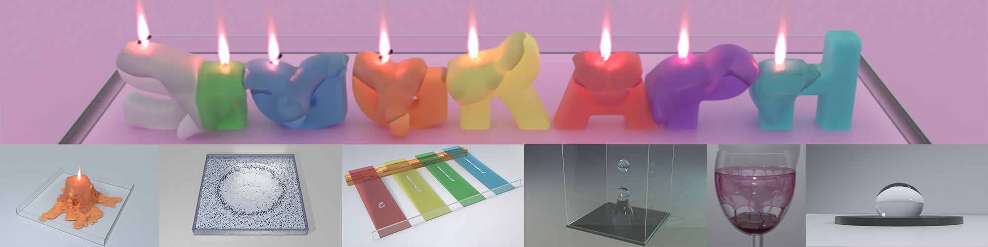
Figure 1. Our method enables the simulation of a wide variety of thermomechanical and surface-tension-driven effects. (Top) Letter-shaped candles melt and interact. (Bottom) A large melting candle; soap spreading on a water surface; water droplets falling and streaking on ramps; partial rebound of a water droplet impact; wine settling in a glass; a water droplet settling on a hydrophobic surface.

A Momentum-Conserving Implicit Material Point Method for Surface Energies with Spatial Gradients

Abstract.

We present a novel Material Point Method (MPM) discretization of surface tension forces that arise from spatially varying surface energies. These variations typically arise from surface energy dependence on temperature and/or concentration. Furthermore, since the surface energy is an interfacial property depending on the types of materials on either side of an interface, spatial variation is required for modeling the contact angle at the triple junction between a liquid, solid and surrounding air. Our discretization is based on the surface energy itself, rather than on the associated traction condition most commonly used for discretization with particle methods. Our energy based approach automatically captures surface gradients without the explicit need to resolve them as in traction condition based approaches. We include an implicit discretization of thermomechanical material coupling with a novel particle-based enforcement of Robin boundary conditions associated with convective heating. Lastly, we design a particle resampling approach needed to achieve perfect conservation of linear and angular momentum with Affine-Particle-In-Cell (APIC) (Jiang et al., 2015). We show that our approach enables implicit time stepping for complex behaviors like the Marangoni effect and hydrophobicity/hydrophilicity. We demonstrate the robustness and utility of our method by simulating materials that exhibit highly diverse degrees of surface tension and thermomechanical effects, such as water, wine and wax.

1. Introduction

Surface tension driven flows like those in milk crowns (Zheng et al., 2015), droplet coalescence (Thürey et al., 2010; Wojtan et al., 2010; Da et al., 2016; Yang et al., 2016a; Li et al., 2020) and bubble formation (Zhu et al., 2014; Da et al., 2015; Huang et al., 2020) comprise some of the most visually compelling fluid motions. Although these effects are most dominant at small scales, increasing demand for realism in computer graphics applications requires modern solvers capable of resolving them. Indeed surface tension effects have been well examined in the computer graphics and broader computational physics literature. We design a novel approach for simulating surface tension driven phenomena that arise from spatial variations in cohesion and adhesion forces at the interface between two liquids. This is often called the Marangoni effect (Scriven and Sternling, 1960; Venerus and Simavilla, 2015) and perhaps the most famous example is the tears of wine phenomenon (Thomson, 1855). Other notable examples of the Marangoni effect include repulsive flows induced by a soap droplet on a water surface as well as the dynamics of molten waxes and metals (Langbein, 2002; Farahi et al., 2004).

The spatial variation in the surface forces can be characterized in terms of the potential energy $\Psi^{s}$ associated with surface tension:

(1) $$\Psi^{s}=\int_{\Gamma}k^{\sigma}(\mathbf{x})ds(\mathbf{x}).$$

Here the surface tension coefficient $k^{\sigma}$ is proportionate to the relative cohesion and adhesion at the interface between the two fluids. Typically this coefficient is constant across the multi-material interface $\Gamma$, however with the Marangoni effect the coefficient varies with $\mathbf{x}\in\Gamma$. These variations are typically driven by temperature or concentration gradients and give rise to many subtle, but important visual behaviors where the variation typically causes fluid to flow away from low surface energy regions towards high surface energy regions. For example with tears of wine, the spatial variations in the surface energy arise from inhomogeneity in the mixture of alcohol and water caused by the comparatively rapid evaporation of alcohol and high surface tension of water.

There are many existing techniques in the computational physics literature that resolve spatial variations in the surface tension. For particle-based methods like Smoothed Particle Hydrodynamics (SPH) (Monaghan, 1992) and Particle-In-Cell (PIC) (Harlow and Welch, 1965), most of these approaches are based on the Continuum Surface Force (CSF) model of Brackbill et al. (1992). Marangoni effects have not been addressed in computer graphics, other than by Huang et al. (2020) where it was examined for material flows in soap films. To capture the Marangoni effect, most approaches do not work with the potential energy $\Psi^{s}$ in Equation (1) but instead base their discretization on its first variation. This variation results in the interfacial traction condition

(2) $$\mathbf{t} =k^{\sigma}\kappa\mathbf{n}+\nabla^{S}k^{\sigma}.$$

Here $\mathbf{t}$ is the force per unit area due to surface tension at the interface $\Gamma$, $\nabla^{S}$ is the surface gradient operator at the interface and $\kappa$ and $\mathbf{n}$ are the interfacial mean curvature and normal, respectively. The original CSF technique of Brackbill et al. (1992) resolves the mean curvature term in Equation (2), but not the surface gradient term. Tong and Browne (2014) show that the CSF approach can be modified to resolve the surface gradient. However, while this and other other existing approaches in the SPH and PIC literature are capable of resolving the spatial variation, none support implicit time stepping for the surface tension forces.

We build on the work of Hyde et al. (2020) and show that efficient implicit time stepping with Marangoni effects is achievable with PIC. As in Hyde et al. (2020) we observe that similarities with hyperelasticity suggest that the Material Point Method (MPM) (Sulsky et al., 1994) is the appropriate version of PIC. We show that by building our discretization from the energy in Equation (1) rather than the more commonly adopted traction condition in Equation (2), we can naturally compute the first and second variations of the potential needed when setting up and solving the nonlinear systems of equations associated with fully implicit temporal discretization. Interestingly, by basing our discretization on the energy in Equation (1), we also show that no special treatment is required for the interfacial spatial gradient operator $\nabla^{s}$ as was done in e.g. (Tong and Browne, 2014). Furthermore, we show that our approach to discretizing the Marangoni forces can also be used to impose the contact angle at liquid/solid/air interfaces (Young, 1805). We show that this naturally allows for simulation of droplet streaking effects.

While our method is a generalization of the MPM technique in Hyde et al. (2020), we also improve on its core functionality. The Hyde et al. (2020) approach is characterized by the introduction of additional surface tension particles at each time step which are designed to represent the liquid interface $\Gamma$ and its area weighted boundary normals. These surface tension particles are temporary and are deleted at the end of the time step to prevent excessive growth in particle count or macroscopic particle resampling. However, the surface tension particles are massless to prevent violation of conservation of particle mass and momentum. We show that this breaks perfect conservation of grid linear and angular momentum when particles introduce grid nodes with no mass that the surface tension forces will act upon. This is an infrequent occurrence, but breaks the otherwise perfect conservation of grid linear and angular momentum expected with conservative MPM forces. We design a novel mass and momentum resampling technique that, with the introduction of two new types of temporary particles, can restore perfect conservation of grid linear and angular momentum. We call these additional temporary particles balance particles. We show that our novel resampling provides improved behavior over the original approach of Hyde et al. (2020), even in the case of standard, non-Marangoni surface tension effects. Furthermore, although other resampling techniques exists for PIC methods (Edwards and Bridson, 2012; Yue et al., 2015; Gao et al., 2017b), we note that ours is the first to guarantee perfect conservation when using generalized particle velocities associated with the Affine Particle-in-Cell (APIC) method (Jiang et al., 2016, 2015; Fu et al., 2017).

Since variations in surface energy are typically based on temperature and/or concentration gradients, we couple our surface tension coefficients with thermodynamically driven quantities. Furthermore, we resolve solid to liquid and liquid to solid phase changes as a function of temperature since many Marangoni effects arise from melting and cooling. Notably, we show that our novel conservative resampling naturally improves discretization of Robin and Neumann boundary conditions on the interface $\Gamma$ needed for convection/diffusion of temperature and concentration. In summary, our primary contributions are:

• A novel implicit MPM discretization of spatially varying surface tension forces.

• A momentum-conserving particle resampling technique for particles near the surface tension liquid interface.

• An implicit MPM discretization of the convection/diffusion evolution of temperature/concentration coupled to the surface tension coefficient including a novel particle-based Robin boundary condition.

Figure 2. Splitting. After surface particles (yellow) are created, the mass and momentum of the interior MPM particles (blue) that are closest to the surface particles are immediately distributed. Particles in each particle group are assigned equal mass. MPM particles (black) that are not paired with any surface particles remain intact for the splitting process. Surface particles (yellow) and balance particles (red) are assigned the same linear velocity and affine velocity of the original particle (blue).

2. Related Work

We discuss relevant particle-based techniques for simulating Marangoni and surface tension effects, contact angle imposition, thermodynamic evolution of temperature and/or concentration, as well as resampling techniques in particle-based methods.

Particle Methods:

Particle-based methods are very effective for computer graphics applications requiring discretization of surface tension forces. Hyde et al. (2020) provide a thorough discussion of the state of the art. Our approach utilizes the particle-based MPM (Sulsky et al., 1994; de Vaucorbeil et al., 2020) PIC technique, largely due to its natural ability to handle self collision (Guo et al., 2018; Jiang et al., 2017; Fei et al., 2018, 2017), topology change (Wang et al., 2019; Wolper et al., 2020; Wolper et al., 2019), diverse materials (Yue et al., 2015; Stomakhin et al., 2013; Ram et al., 2015; Daviet and Bertails-Descoubes, 2016; Wang et al., 2020c; Klár et al., 2016; Schreck and Wojtan, 2020) as well as implicit time stepping with elasticity (Stomakhin et al., 2013; Fei et al., 2018; Wang et al., 2020b; Fang et al., 2019). We additionally use the APIC method (Jiang et al., 2016, 2015; Fu et al., 2017) for its conservation properties and beneficial suppression of noise. Note that our mass and momentum remapping technique is designed to work in the context of the APIC techniques where particles store generalized velocity information.

SPH is very effective for resolving Marangoni effects. The approaches of Tong and Browne (2014) and Hopp-Hirschler et al. (2018) are indicative of the state of the art. Most SPH works rely on the CSF surface tension model of Brackbill et al. (1992), which transforms surface tension traction into a volumetric force that is only non-zero along (numerically smeared) material interfaces. CSF approaches generally derive surface normal and curvature estimates as gradients of color functions, which can be very sensitive to particle distribution. Also, CSF forces are not exactly conservative (Hyde et al., 2020). SPH can also be used to simulate the convection and diffusion of temperature/concentration that gives rise to the spatial variation in surface energy in the Marangoni effect. Hu and Eberhard (2017) simulate Marangoni convection in a melt pool during laser welding and Russell (2018) does so in laser fusion additive manufacturing processes. Both approaches use SPH with Tong and Browne (2014) for discretization of Equation (2). Although SPH is very effective for resolving Marangoni effects, all existing approaches utilize implicit treatment of Marangoni forces.

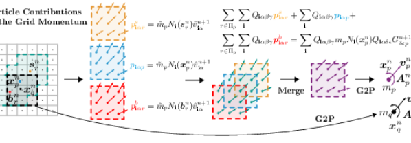
Figure 3. Merging. The merging process is a modified version of G2P. For the particles that are not associated with surface particles (black), a regular G2P is performed. Among each particle group, we calculate each particle’s contribution to the grid momentum and the generalized affine moments of their summed momenta about their center of mass. Then, we restore the mass of the original particle associated with the group prior to the split and compute its generalized affine inertia tensor from its grid mass distribution. Using the affine inertia tensor of the original particle, we compute generalized velocity of the particle after the merging from the generalized moments of the group.

Marangoni effect and contact angle:

The Marangoni effect is visually subtle and has not been resolved with particle-based methods in computer graphics applications. Perhaps the most visually compelling example of the Marangoni effect is the tears of wine phenomenon on the walls of a wine glass (Scriven and Sternling, 1960; Venerus and Simavilla, 2015). Tears of wine were simulated in Azencot et al. (2015), however the authors modeled the fluid using thin film equations under the lubrication approximation and did not model surface tension gradients. The fingering instabilities they observed are stated to occur due to the asymmetric nature of their initial conditions. The Marangoni effect was resolved by Huang et al. (2020) recently with thin soap films to generate compelling dynamics of the characteristic rainbow patterns in bubbles. Relatedly, Ishida et al. (2020) simulated the evolution of soap films including effects of thin-film turbulence, draining, capillary waves, and evaporation. Outside of computer graphics, the Marangoni effect has been recently studied in works like Dukler et al. (2020), which models undercompressive shocks in the Marangoni effect, and de Langavant et al. (2017), which presents a spatially-adaptive level set approach for simulating surfactant-driven flows. Also, Nas and Tryggvason (2003) simulated thermocapillary motion of bubbles and drops in flows with finite Marangoni numbers (flows with significant transport due to Marangoni effects).

Our approach for the Marangoni effect also allows for imposition of contact angles at air/liquid/solid interfaces. This effect is important for visual realism when simulating droplets of water in contact with solid objects like the ground. Contact angles are influenced by the hydrophilicity/hydrophobicity of the surface on which these droplets move or rest (Cassie and Baxter, 1944; Johnson Jr. and Dettre, 1964). Wang et al. (2007) solve General Shallow Wave Equations, including surface tension boundary conditions and the virtual surface method of Wang et al. (2005), in order to model contact angles and hydrophilicity. Yang et al. (2016b) use a pairwise force model (Tartakovsky and Meakin, 2005) for handling contact angles in their SPH treatment of fluid-fluid and solid-fluid interfaces. Clausen et al. (2013) also consider the relation between surface tension and contact angles in their Lagrangian finite element approach.

Particle Resampling:

Reseeding or resampling particles is a common concern in various simulation methods; generally speaking, particles need to be distributed with sufficient density near dynamic areas of flow or deformation in order to accurately resolve the dynamics of the system (Ando et al., 2012; Losasso et al., 2008; Narain et al., 2010). Edwards and Bridson (2012) use a non-conservative random sampling scheme to seed and reseed particles with PIC. Pauly et al. (2005) resample to preserve detail near cracks/fracture, but their resampling does not attempt to conserve momentum. Yue et al. (2015) use Poisson disk sampling to insert new points in low-density regions and merge points that are too close to one another with MPM. However, their resampling method is not demonstrated to be momentum-conserving. A conservative variant of this split-and-merge approach is applied in Gao et al. (2017b) where mass and linear momentum are conserved during particle splitting and merging. However, angular momentum conservation is not conserved. Furthermore, these techniques use PIC not APIC and neither is designed to guarantee conservation with the generalized velocity state in APIC techniques (Jiang et al., 2016, 2015; Fu et al., 2017).

Thermomechanical Effects:

Thermodynamic effects in visual simulation date back to at least Terzopoulos et al. (1991). More recently, melting and resolidification for objects like melting candles have been simulated using various methods, including Lattice Boltzmann (Wang et al., 2012) and SPH (Paiva et al., 2009; Lenaerts and Dutré, 2009), though these results leave room for improved visual and physical fidelity. FLIP methods have also been used for thermodynamic problems, such as Gao et al. (2017a), which adapts the latent heat model from Stomakhin et al. (2014). Condensation and evaporation of water were considered in several works based on SPH (Hochstetter and Kolb, 2017; Zhang et al., 2017). SPH was also applied to the problem of simulating boiling bubbles in Gu and Yang (2016), which models heat conduction, convection and mass transfer. Recently, particle-based thermodynamics models were incorporated into an SPH snow solver (Gissler et al., 2020a), with temperature-dependent material properties such as the Young’s modulus. In another vein, Pirk et al. (2017) used position-based dynamics and Cosserat physics to simulate combustion of tree branches, including models for moisture and charring. Yang et al. (2017) used the Cahn-Hilliard and Allen-Cahn equations to evolve a continuous phase variable for materials treated with their phase-field method. Maeshima et al. (2020) considered particle-scale explicit MPM modeling for additive manufacturing (selective laser sintering) that included a latent heat model for phase transition. For a detailed review of thermodynamical effects in graphics, we refer the reader to Stomakhin et al. (2014).

Surface Tension:

Many methods for simulating non-Marangoni surface tension effects have been developed for computer graphics applications. We refer the reader to Hyde et al. (2020) for a detailed survey. More recently, Chen et al. (2020) incorporated sub-cell-accurate surface tension forces in an Eulerian fluid framework based on integrating the mean curvature flow of the liquid interface (following Sussman and Ohta (2009)). With an eye towards resolving codimensional flow features, such as thin sheets and filaments, Wang et al. (2020a) and Zhu et al. (2014) simulated surface tension forces using moving-least-squares particles and simplicial complexes, respectively. Most related to the present work, Hyde et al. (2020) proposed an implicit material point method for simulating liquids with large surface energy, such as liquid metals. Their surface tension formulation follows (Adamson and Gast, 1967; Brackbill et al., 1992; Buscaglia and Ausas, 2011) and incorporates a potential energy associated with surface tension into the MPM framework. Material boundaries are sampled using massless MPM particles.

3. Governing Equations

We first define the governing equations for thermomechanically driven phase change of hyperelastic solids and liquids with variable surface energy. As in Hyde et al. (2020) we also cover the updated Lagrangian kinematics. Lastly, we provide the variational form of the governing equations for use in MPM discretization. We note that throughout the document Greek subscripts are assumed to run from $0,1,\ldots,d-1$ for the dimension $d=2,3$ of the problem. Repeated Greek subscripts imply summation, while sums are explicitly indicated for Latin subscripts. Also, Latin subscripts in bold are used for multi-indices.

3.1. Kinematics

We adopt the continuum assumption (Gonzalez and Stuart, 2008) and updated Lagrangian kinematics (Belytschko et al., 2013) used in Hyde et al. (2020). At time $t$ we associate our material with subsets $\Omega^{t}\subset\mathbb{R}^{d}$, $d=2,3$. We use $\Omega^{0}$ to denote the initial configuration of material with $\mathbf{X}\in\Omega^{0}$ used to denote particles of material at time $t=0$. A flow map $\boldsymbol{\phi}:\Omega^{0}\times[0,T]\rightarrow\mathbb{R}^{d}$ defines the material motion of particles $\mathbf{X}\in\Omega^{0}$ to their time $t$ locations $\mathbf{x}\in\Omega^{t}$ as $\boldsymbol{\phi}(\mathbf{X},t)=\mathbf{x}$. The Lagrangian velocity is defined by differentiating the flow map in time $\mathbf{V}(\mathbf{X},t)=\frac{\partial\boldsymbol{\phi}}{\partial t}(\mathbf{X},t)$.

3.1.1. Eulerian and Updated Lagrangian Representations

The Lagrangian velocity can be difficult to work with in practice since real world observations of material are made in $\Omega^{t}$ not $\Omega^{0}$. The Eulerian velocity $\mathbf{v}:\Omega^{t}\rightarrow\mathbb{R}^{d}$ is what we observe in practice. The Eulerian velocity is defined in terms of the inverse flow map $\boldsymbol{\phi}^{-1}(\cdot,t):\Omega^{t}\rightarrow\Omega^{0}$ as $\mathbf{v}(\mathbf{x},t)=\mathbf{V}(\boldsymbol{\phi}^{-1}(\mathbf{x},t),t)$ where $\boldsymbol{\phi}^{-1}(\mathbf{x},t)=\mathbf{X}$. In general, we can use the flow map and its inverse to pull back quantities defined over $\Omega^{t}$ and push forward quantities defined over $\Omega^{0}$, respectively. For example, given $G:\Omega^{0}\rightarrow\mathbb{R}$, its push forward $g:\Omega^{t}\rightarrow\mathbb{R}$ is defined as $g(\mathbf{x})=G(\boldsymbol{\phi}^{-1}(\mathbf{x},t))$. This process is related to the material derivative operator $\frac{D}{Dt}$ where $\frac{Dg}{Dt}(\mathbf{x},t)=\frac{\partial G}{\partial t}(\boldsymbol{\phi}^{-1}(\mathbf{x},t))=\frac{\partial g}{\partial t}(\mathbf{x},t)+\sum_{\alpha=0}^{d-1}\frac{\partial g}{\partial x_{\alpha}}(\mathbf{x},t)v_{\alpha}(\mathbf{x},t)$ (see e.g. (Gonzalez and Stuart, 2008) for more detail).

In the updated Lagrangian formalism (Belytschko et al., 2013) we write quantities over an intermediate configuration of material $\Omega^{s}$ with $0\leq s<t$. For example, we can define $\hat{g}(\cdot,s):\Omega^{s}\rightarrow\mathbb{R}$ as $\hat{g}(\tilde{\mathbf{x}},s)=G(\boldsymbol{\phi}^{-1}(\tilde{\mathbf{x}},s))$ for $\tilde{\mathbf{x}}\in\Omega^{s}$. As shown in Hyde et al. (2020), this is particularly useful when discretizing momentum balance using its variational form. The key observation is that the updated Lagrangian velocity can be written as $\hat{\mathbf{v}}(\tilde{\mathbf{x}},s,t)=\mathbf{V}(\boldsymbol{\phi}^{-1}(\tilde{\mathbf{x}},s),t)=\mathbf{v}(\hat{\boldsymbol{\phi}}(\tilde{\mathbf{x}},s,t),t)$ with $\hat{\boldsymbol{\phi}}(\tilde{\mathbf{x}},s,t)=\boldsymbol{\phi}(\boldsymbol{\phi}^{-1}(\tilde{\mathbf{x}},s),t))$ for $\tilde{\mathbf{x}}\in\Omega^{s}$. Intuitively, $\hat{\boldsymbol{\phi}}(\cdot,s,t):\Omega^{s}\rightarrow\Omega^{t}$ is the mapping from the time $s$ configuration to the time $t$ configuration induced by the flow map. This has a simple relation to the material derivative as $\frac{\partial\hat{\mathbf{v}}}{\partial t}(\tilde{\mathbf{x}},s,t)=\frac{\partial\mathbf{V}}{\partial t}(\boldsymbol{\phi}^{-1}(\tilde{\mathbf{x}},s),t)=\frac{D\mathbf{v}}{Dt}(\hat{\boldsymbol{\phi}}(\tilde{\mathbf{x}},s,t),t)$. As in Hyde et al. (2020) we will generally use upper case for Lagrangian quantities, lower case for Eulerian quantities and hat superscripts for updated Lagrangian quantities.

3.1.2. Deformation Gradient

The deformation gradient $\mathbf{F}=\frac{\partial\boldsymbol{\phi}}{\partial\mathbf{X}}$ is defined by differentiating the flow map in space and can be used to quantify the amount of deformation local to a material point. We use $J=\det(\mathbf{F})$ to denote the deformation gradient determinant. $J$ represents the amount of volumetric dilation at a material point. Furthermore, it is used when changing variables with integration. We also make use of similar notation for the $\hat{\boldsymbol{\phi}}$ mapping from $\Omega^{s}$ to $\Omega^{t}$, i.e. $\hat{\mathbf{F}}=\frac{\partial\hat{\boldsymbol{\phi}}}{\partial\tilde{\mathbf{x}}}$, $\hat{J}=\det\big(\hat{\mathbf{F}}\big{missing})$.

3.2. Conservation of Mass and Momentum

Our governing equations primarily consist of conservation of mass and momentum which can be expressed as

(3) $$\rho\frac{D\mathbf{v}}{Dt} =\nabla\cdot\boldsymbol{\sigma}+\rho\mathbf{g},\ \frac{D\rho}{Dt}=-\rho\nabla\cdot\mathbf{v},\ \mathbf{x}\in\Omega^{t}$$

where $\rho$ is the Eulerian mass density, $\mathbf{v}$ is the Eulerian material velocity, $\boldsymbol{\sigma}$ is the Cauchy stress and $\mathbf{g}$ is gravitational acceleration. Boundary conditions for these equations are associated with a free surface for solid material, surface tension for liquids and/or prescribed velocity conditions. We use $\partial\Omega^{t}_{N}$ to denote the portion of the time $t$ boundary subject to free surface or surface tension conditions and $\partial\Omega^{t}_{D}$ to denote the portion of the boundary with Dirichlet velocity boundary conditions. Free surface conditions and surface tension boundary conditions are expressed as

(4) $$\boldsymbol{\sigma}\mathbf{n}=\mathbf{t},\mathbf{x}\in\partial\Omega^{t}_{N}$$

where $\mathbf{t}=\mathbf{0}$ for free surface conditions and $\mathbf{t}=k^{\sigma}\kappa\mathbf{n}+\nabla^{S}k^{\sigma}$ from Equation (2) for surface tension conditions. Velocity boundary conditions may be written as

(5) $$\mathbf{v}\cdot\mathbf{n}=v_{\text{bc}}^{n},\mathbf{x}\in\partial\Omega_{D}^{t}.$$

3.2.1. Constitutive Models

Each material point is either a solid or liquid depending on the thermomechanical evolution. For liquids, the Cauchy stress $\boldsymbol{\sigma}$ is defined in terms of pressure and viscous stress:

$$\boldsymbol{\sigma}=-p\mathbf{I}+\mu\left(\frac{\partial\mathbf{v}}{\partial\mathbf{x}}+\frac{\partial\mathbf{v}}{\partial\mathbf{x}}^{T}\right),\ p=-\frac{\partial\Psi^{p}}{\partial J},$$

with $\Psi^{p}(J)=\frac{\lambda^{l}}{2}(J-1)^{2}$. Here $\lambda^{l}$ is the bulk modulus of the liquid and $\mu^{l}$ is its viscosity. For solids, the Cauchy stress is defined in terms of a hyperelastic potential energy density $\Psi^{s}$ as

$$\boldsymbol{\sigma}=\frac{1}{j}\frac{\partial\psi^{h}}{\partial\mathbf{F}}\mathbf{f}^{T}$$

where $\mathbf{f}(\mathbf{x},t)=\mathbf{F}(\boldsymbol{\phi}^{-1}(\mathbf{x},t),t)$ and $j(\mathbf{x},t)=J(\boldsymbol{\phi}^{-1}(\mathbf{x},t),t)$ are the Eulerian deformation gradient and its determinant, respectively. We use the fixed-corotated constitutive model from (Stomakhin et al., 2012) for $\psi^{h}$. This model is defined in terms of the polar SVD (Irving et al., 2004) of the deformation gradient $\mathbf{F}=\mathbf{U}\boldsymbol{\Sigma}\mathbf{V}^{T}$ with

$$\psi^{h}(\mathbf{F})=\mu^{h}\sum_{\alpha=0}^{d-1}(\sigma_{\alpha}-1)^{2}+\frac{\lambda^{h}}{2}(J-1)^{2},$$

where the $\sigma_{\alpha}$ are the diagonal entries of $\boldsymbol{\Sigma}$ and $\mu^{h},\lambda^{h}$ are the hyperelastic Lamé coefficients.

3.3. Conservation of energy

We assume the internal energy of our materials consists of potential energy associated with surface tension, liquid pressure and hyperelasticity and thermal energy associated with material temperature. Conservation of energy together with thermodynamic considerations requires convection/diffusion of the material temperature (Gonzalez and Stuart, 2008) subject to Robin boundary conditions associated with convective heating by ambient material:

(6) $$\rho c_{p}\frac{DT}{Dt} =K\Delta T+H$$

$$K\gradient T\cdot\mathbf{n} =-h(T-\bar{T})+b.$$

Here $c_{p}$ is specific heat capacity, $T$ is temperature, $K$ is thermal diffusivity, $H$ is a source function, $\bar{T}$ is the temperature of ambient material and $\mathbf{n}$ is the surface boundary normal. $h$ controls the rate of convective heating to the ambient temperature and $b$ represents the rate of boundary heating independent of the ambient material temperature $\bar{T}$.

The total potential energy $\Psi$ in our material is as in Hyde et al. (2020), however we include the spatial variation of the surface energy density in Equation (1) and the hyperelastic potential for solid regions:

$$\Psi(\boldsymbol{\phi}(\cdot,t))=\Psi^{\sigma}(\boldsymbol{\phi}(\cdot,t))+\Psi^{l}(\boldsymbol{\phi}(\cdot,t))+\Psi^{h}(\boldsymbol{\phi}(\cdot,t))+\Psi^{g}(\boldsymbol{\phi}(\cdot,t)).$$

Here $\Psi^{\sigma}$ is the potential from surface tension, $\Psi^{l}$ is the potential from liquid pressure, $\Psi^{h}$ is the potential from solid hyperelasticity and $\Psi^{g}$ is the potential from gravity. As in typical MPM discretizations, our approach is designed in terms of these energies:

$$\Psi^{g}(\boldsymbol{\phi}(\cdot,t) =\int_{\Omega^{0}}R\mathbf{g}\cdot\boldsymbol{\phi}Jd\mathbf{X},\ \Psi^{\sigma}(\boldsymbol{\phi}(\cdot,t))=\int_{\partial\Omega^{t}}k^{\sigma}(\mathbf{x},t)ds(\mathbf{x})$$

$$\ \Psi^{l}(\boldsymbol{\phi}(\cdot,t)) =\int_{\Omega^{0}}\frac{\lambda^{l}}{2}\left(J-1\right)^{2}d\mathbf{X},\ \Psi^{h}(\boldsymbol{\phi}(\cdot,t))=\int_{\Omega^{0}}\psi^{h}(\mathbf{F})d\mathbf{X}.$$

Here $R$ is the pull back (see Section 3.1) of the mass density $\rho$. Note that in the expression for the surface tension potential it is useful to change variables using the updated Lagrangian view as in Hyde et al. (2020):

(7) $$\Psi^{\sigma}(\boldsymbol{\phi}(\cdot,t)) =\int_{\partial\Omega^{t}}k^{\sigma}(\mathbf{x},t)ds(\mathbf{x})=\int_{\partial\Omega^{s}}k^{\sigma}(\hat{\boldsymbol{\phi}}(\tilde{\mathbf{x}},s,t),t)|\hat{J}\hat{\mathbf{F}}^{-T}\tilde{\mathbf{n}}|ds(\tilde{\mathbf{x}}).$$

Here $\tilde{\mathbf{n}}$ is the outward unit normal at a point on the boundary of $\Omega^{s}$ and the expression $ds(\mathbf{x})=|\hat{J}\hat{\mathbf{F}}^{-T}\tilde{\mathbf{n}}|ds(\tilde{\mathbf{x}})$ arises by a change of variables from an integral over $\Omega^{t}$ to one over $\Omega^{s}$. Notably, the spatial variation in $k^{\sigma}$ does not require a major modification of the Hyde et al. (2020) approach.

3.4. Variational Form of Momentum Balance

The strong form of momentum balance in Equation (3), together with the traction (Equation (4)) and Dirichlet velocity boundary conditions (Equation (5)), is equivalent to a variational form that is useful when discretizing our governing equations using MPM. To derive the variational form, we take the dot product of Equation (3) with an arbitrary function $\mathbf{w}:\Omega^{t}\rightarrow\mathbb{R}^{d}$ satisfying $\mathbf{w}\cdot\mathbf{n}=0$ for $\mathbf{x}\in\partial\Omega^{t}_{D}$ and integrate over the domain $\Omega^{t}$, applying integration by parts where appropriate. Requiring that the Dirichlet velocity conditions in Equation (4) hold together with the following integral equations for all functions $\mathbf{w}$ is equivalent to the strong form, assuming sufficient solution regularity:

(8) $$\int_{\Omega^{t}}\rho\frac{Dv_{\alpha}}{Dt}w_{\alpha}d\mathbf{x}=-\frac{d}{d\epsilon}PE(0;\mathbf{w})-\mu^{l}\int_{\Omega^{t}}\epsilon^{v}_{\alpha\beta}\epsilon^{w}_{\alpha\beta}d\mathbf{x}.$$

Here $\epsilon^{w}=\frac{1}{2}\left(\frac{\partial w_{\alpha}}{\partial x_{\beta}}+\frac{\partial w_{\beta}}{\partial x_{\alpha}}\right)$ and $\epsilon^{v}=\frac{1}{2}\left(\frac{\partial v_{\alpha}}{\partial x_{\beta}}+\frac{\partial v_{\beta}}{\partial x_{\alpha}}\right)$ and

$$\textrm{PE}(\epsilon;\mathbf{w})=\Psi(\boldsymbol{\phi}(\cdot,t)+\epsilon\mathbf{W}).$$

Here $\mathbf{W}$ is the pull back of $\mathbf{w}$ (see Section 3.1). Note that this notation is rather subtle for the surface tension potential energy. For clarification,

$$\Psi^{\sigma}(\boldsymbol{\phi}(\cdot,t)+\epsilon\mathbf{W}) =\int_{\partial\Omega^{s}}k^{\sigma}(\hat{\boldsymbol{\phi}}+\epsilon\hat{\mathbf{w}})|\hat{J}_{\epsilon,\hat{\mathbf{w}}}\hat{\mathbf{F}}_{{}^{\epsilon,\hat{\mathbf{w}}}}^{-T}\tilde{\mathbf{n}}|ds(\tilde{\mathbf{x}}),$$

where $\hat{\mathbf{w}}(\tilde{\mathbf{x}},s,t)=\mathbf{w}(\hat{\boldsymbol{\phi}}(\tilde{\mathbf{x}},s,t))$ is the updated Lagrangian pull back of $\mathbf{w}$, $\hat{\mathbf{F}}_{{}^{\epsilon,\hat{\mathbf{w}}}}=\frac{\partial\hat{\boldsymbol{\phi}}+\epsilon\hat{\mathbf{w}}}{\partial\tilde{\mathbf{x}}}$ is the deformation gradient of the mapping $\hat{\boldsymbol{\phi}}+\epsilon\hat{\mathbf{w}}$ and $\hat{J}_{\epsilon,\hat{\mathbf{w}}}=\det\big(\hat{\mathbf{F}}_{{}^{\epsilon,\hat{\mathbf{w}}}}\big{missing})$ is its determinant. Lastly, for discretization purposes, in practice we change variables in the viscosity term

(9) $$\mu^{l}\int_{\Omega^{t}}\epsilon^{v}_{\alpha\beta}\epsilon^{w}_{\alpha\beta}d\mathbf{x}=\mu^{l}\int_{\Omega^{s}}\hat{\epsilon}^{v}_{\alpha\beta}\hat{\epsilon}^{w}_{\alpha\beta}\hat{J}d\tilde{\mathbf{x}}.$$

We can similarly derive a variational form of the temperature evolution in Equation (6) by requiring

(10) $$\int_{\Omega_{t}}\rho c_{p}\frac{DT}{Dt}qd\mathbf{x}= -\int_{\partial\Omega_{t}}qhTd\SS(\mathbf{x})+\int_{\partial\Omega_{t}}q\left(h\bar{T}+b\right)d\SS(\mathbf{x})$$

$$+\int_{\Omega_{t}}Hqd\mathbf{x}-\int_{\Omega_{t}}\gradient{q}\cdot K\gradient{T}d\mathbf{x}$$

for all functions $q:\Omega^{t}\rightarrow\mathbb{R}$.

3.5. Thermomechanical Material Dependence and Phase Change

The thermomechanical material dependence is modeled by allowing the surface tension coefficient $k^{\sigma}$, the liquid bulk modulus $\lambda^{l}$, the liquid viscosity $\mu^{l}$ and the hyperelastic Lamé coefficients $\mu^{h},\lambda^{h}$ to vary with temperature. When $T$ exceeds a user-specified melting point $T_{\text{melt}}$, the solid phase is changed to liquid and the deformation gradient determinant $J$ is set to $1$. Similarly, if liquid temperature drops below $T_{\text{melt}}$, The phase is updated to be hyperelastic solid and the deformation gradient $\mathbf{F}$ is set to the identity matrix. In practice, resetting the deformation gradient and its determinant helps to prevent nonphysical popping when the material changes from solid to liquid and vice versa. We remark that incorporating a more sophisticated phase change model, such as a latent heat buffer, is potentially useful in future work (Stomakhin et al., 2014).

3.6. Contact Angle

The contact angle between a liquid, a solid boundary and the ambient air is governed by the Young equation (Young, 1805). This expression relates the resting angle $\theta$ (measured through the liquid) of a liquid in contact with a solid surface to the surface tension coefficients between the liquid, solid and air phases:

(11) $$k^{\sigma}_{SG}=k^{\sigma}_{SL}+k^{\sigma}_{LG}\cos(\theta).$$

The surface tension coefficients are between the solid and gas phases, solid and liquid phases, and liquid and gas phases, respectively. As in Clausen et al. (2013), we assume $k^{\sigma}_{SG}$ is negligible since we are using a free surface assumption and do not explicitly model the air. Under this assumption, the solid-liquid contact angle is determined by the surface tension ratio $-k^{\sigma}_{SL}/k^{\sigma}_{LG}$. We note that, while one would expect surface tension coefficients/energies to be positive, this ratio can be negative under the assumption of zero solid-gas surface tension. Furthermore, we note that utilizing this expression requires piecewise constant surface tension coefficients where the variation along the liquid boundary is based on which portion is in contact with the air and which is in contact with the solid. The distinct surface tension coefficients on different interfaces provide controllability of the spreading behavior of the liquid on the solid surface.

4. Discretization

As in Hyde et al. (2020), we use MPM (Sulsky et al., 1994) and APIC (Jiang et al., 2015) to discretize the governing equations. The domain $\Omega^{t^{n}}$ at time $t^{n}$ is sampled using material points $\mathbf{x}_{p}^{n}$. These points also store approximations of the deformation gradient determinant $J_{p}^{n}$, constant velocity $\mathbf{v}_{p}^{n}$, affine velocity $\mathbf{A}_{p}^{n}$, volume $V_{p}^{0}$, mass $m_{p}=\rho(\mathbf{x}_{p}^{0},t^{0})V_{p}^{0}$, temperature $T_{p}^{n}$, and temperature gradient $\gradient T_{p}^{n}$. We also make use of a uniform background grid with spacing $\Delta x$ when discretizing momentum updates. To advance our state to time $t^{n+1}$, we use the following steps:

1. Resample particle boundary for surface tension and Robin boundary temperature conditions.

2. P2G: Conservative transfer of momentum and temperature from particles to grid.

3. Update of grid momentum and temperature.

4. G2P: Conservative transfer of momentum and temperature from grid to particles.

4.1. Conservative Surface Particle Resampling

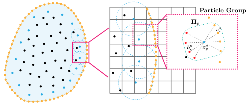
Figure 4. A portion of an MPM fluid in the simulation domain. Surface particles (yellow) are sampled on faces of the zero isocontour of the level set formed by unioning spherical level sets around each MPM particle. Each surface particle generates an associated balance particle (red) such that the closest MPM particle (blue) to a boundary particle lies on the midpoint of a line segment between the surface particle and balance particle. A single blue particle at $\boldsymbol{x}_{p}$ may be paired with multiple surface particles and balance particles, and they are considered to be in a particle group $\boldsymbol{\Pi}_{p}$. MPM particles that are not associated with any surface tension particles are marked as black.

The integrals associated with the surface tension energy in Equation (7) and the Robin temperature condition in Equation (10) are done over the boundary of the domain. We follow Hyde et al. (2020) and introduce special particles to cover the boundary in order to serve as quadrature points for these integrals. As in Hyde et al. (2020) these particles are temporary and are removed at the end of the time step. However, while Hyde et al. (2020) used massless surface particles, we design a novel conservative mass and momentum resampling for surface particles. Massless particles easily allow for momentum conserving transfers from particle to grid and vice versa; however, they can lead to loss of conservation in the grid momentum update step. This occurs when there is a grid cell containing only massless particles. In this case, there are grid nodes with no mass that receive surface tension forces. These force components are then effectively thrown out since only grid nodes with mass will affect the end of time step particle momentum state (see Section 6.1).

We resolve this issue by assigning mass to each of the surface particles. However, to conserve total mass, some mass must be subtracted from interior MPM particles. Furthermore, changing the mass of existing particles also changes their momentum, which may lead to violation of conservation. In order to conserve mass, linear momentum and angular momentum, we introduce a new particle for each surface particle. We call these balance particles, and like surface particles they are temporary and will be removed at the end of the time step. We show that the introduction of these balance particles naturally allows for conservation both when they are created at the beginning of the time step and when they are removed at the end of the time step.

4.1.1. Surface Particle Sampling

We first introduce surface particles using the approach in Hyde et al. (2020). A level set enclosing the interior MPM particles is defined as the union of spherical level sets defined around each interior MPM particle. Unlike Hyde et al. (2020), we do not smooth or shift the unioned level set. We compute the zero isocontour of the level set using marching cubes (Chernyaev, 1995) and randomly sample surface particles along this explicit representation. In Hyde et al. (2020), three-dimensional boundaries were sampled using a number of sample points proportional to the surface area of each triangle. Sample points were computed using uniform random barycentric weights, which leads to a non-uniform distribution of points in each triangle. Instead, we employ a strategy of per-triangle Monte Carlo sampling using a robust Poisson distribution, as described in Corsini et al. (2012), where uniform triangle sample points are generated according to Osada et al. (2002). We found that this gave better coverage of the boundary without generating particles that are too close together (see Figure 5). We note that radii for the particle level sets are taken to be $0.73\Delta x$ (slightly larger than $\frac{\sqrt{2}}{2\Delta x}$) in 2D and $0.867\Delta x$ (slightly larger than $\frac{\sqrt{3}}{2\Delta x}$) in 3D. This guarantees that even a single particle in isolation will always generate a level set zero isocontour that intersects the grid and will therefore always generate boundary sample points. Note also that as in Hyde et al. (2020), we use the explicit marching cubes mesh of the zero isocontour to easily and accurately generate samples of area weighted normals $d\mathbf{A}_{r}$ where $\sum|d\mathbf{A}_{r}|\approx\int_{\Omega}^{t^{n}}d\mathbf{x}$ are chosen with direction from the triangle normal and magnitude based on the number of samples in a given triangle and the triangle area.

4.1.2. Balance Particle Sampling

For each surface particle $\mathbf{s}_{r}^{n}$, we additionally generate a balance particle $\mathbf{b}_{r}^{n}$. First, we compute the closest interior MPM particle for each surface particle $\mathbf{x}_{p(\mathbf{s}_{r}^{n})}^{n}$. Then we introduce the corresponding balance particle as

(12) $$\mathbf{b}_{r}^{n}=\mathbf{s}_{r}^{n}+2\left(\mathbf{x}_{p(\mathbf{s}_{r}^{n})}^{n}-\mathbf{s}_{r}^{n}\right).$$

4.1.3. Mass and Momentum Splitting

After introducing the surface $\mathbf{s}^{n}_{r}$ and balance $\mathbf{b}^{n}_{r}$ particles, we assign them mass and momentum (see Figure 2). To achieve this in a conservative manner, we first partition the surface particles into particle groups $\Pi_{p}$ defined as the set of surface particle indices $r$ such that $\mathbf{x}_{p}^{n}$ is the closest interior MPM particle to $\mathbf{s}^{n}_{r}$ (see Figure (4)). We assign the mass $m_{p}$ of the particle $\mathbf{x}_{p}^{n}$ to the collection of $\mathbf{x}_{p}^{n}$, $\mathbf{s}^{n}_{r}$ and $\mathbf{b}^{n}_{r}$ for $r\in\Pi_{p}$ uniformly by defining a mass of $\tilde{m}_{p}=\frac{m_{p}}{2|\Pi_{p}|+1}$ to each surface and balance point as well as to $\mathbf{x}_{p}^{n}$. Here $|\Pi_{p}|$ is the number of elements in the set. This operation is effectively a split of the original particle $\mathbf{x}_{p}^{n}$ with mass $m_{p}$ into a new collection of particles $\mathbf{x}_{p}^{n},\mathbf{s}^{n}_{r},\mathbf{b}^{n}_{r},\ r\in\Pi_{p}$ with masses $\tilde{m}_{p}$. This split trivially conserves the mass. Importantly, by construction of the balance particles (Equation (12)) we ensure that the center of mass of the collection is equal to the original particle $\mathbf{x}_{p}^{n}$:

(13) $$\frac{1}{m_{p}}\left(\tilde{m}_{p}\mathbf{x}_{p}^{n}+\sum_{r\in\Pi_{p}}\tilde{m}_{p}\mathbf{s}^{n}_{r}+\tilde{m}_{p}\mathbf{b}^{n}_{r}\right)=\mathbf{x}_{p}^{n}.$$

With this particle distribution, conservation of linear and angular momentum can be achieved by simply assigning each new particle in the collection the velocity $\mathbf{v}_{p}^{n}$ and affine velocity $\mathbf{A}_{p}^{n}$ of the original particle $\mathbf{x}_{p}^{n}$. We note that the conservation of the center of mass (Equation (13)) is essential for this simple constant velocity split to conserve linear and angular momentum (see (Annonymous, 2021)).

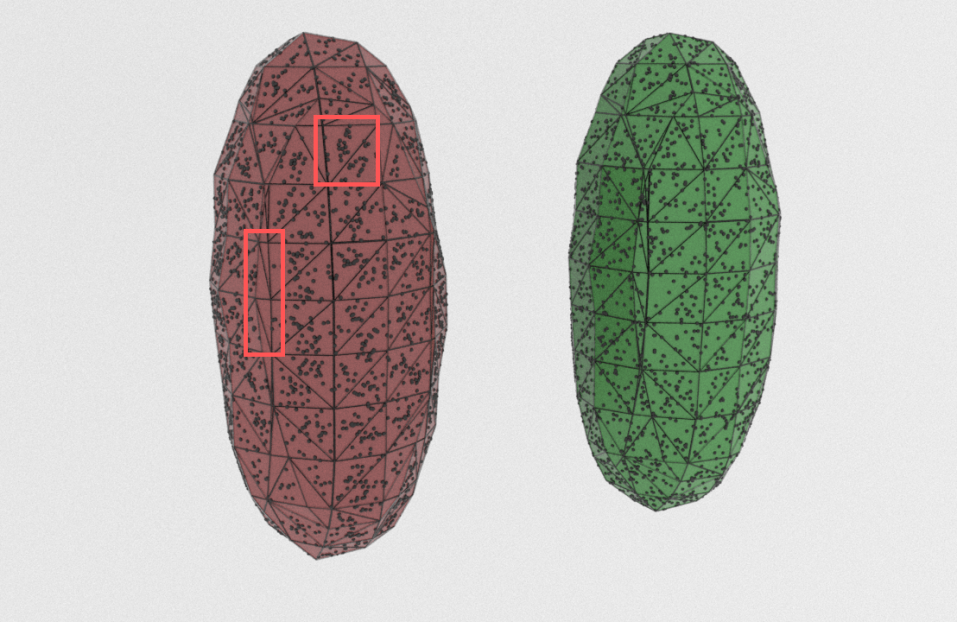
Figure 5. Isocontour and sampled boundary particles for an ellipsoid. (Left) Using the method of Hyde et al. (2020). Note how low-quality triangles are undersampled and how sample points often clump near triangle centers. (Right) The present method, which does not suffer from similar issues.

4.2. Transfer: P2G

After the addition of the surface and balance particles, we transfer mass and momentum to the grid in the standard APIC (Jiang et al., 2015) way using their conservatively remapped mass and velocity state

$$m^{n}_{\mathbf{i}} =\sum_{p}\tilde{m}_{p}\left(N_{\mathbf{i}}(\mathbf{x}^{n}_{p})+\sum_{r\in\Pi_{p}}N_{\mathbf{i}}(\mathbf{s}^{n}_{r})+N_{\mathbf{i}}(\mathbf{b}^{n}_{r})\right),$$

$$\quad m^{n}_{\mathbf{i}}\mathbf{v}^{n}_{\mathbf{i}} =\sum_{p}\tilde{m}_{p}N_{\mathbf{i}}(\mathbf{x}^{n}_{p})\left(\mathbf{v}^{n}_{p}+\mathbf{A}^{n}_{p}(\mathbf{x}_{\mathbf{i}}-\mathbf{x}^{n}_{p})\right)$$

$$+\sum_{p}\tilde{m}_{p}\sum_{r\in\Pi_{p}}N_{\mathbf{i}}(\mathbf{s}^{n}_{r})\left(\mathbf{v}^{n}_{p}+\mathbf{A}^{n}_{p}(\mathbf{x}_{\mathbf{i}}-\mathbf{s}^{n}_{r})\right)$$

$$+\sum_{p}\tilde{m}_{p}\sum_{r\in\Pi_{p}}N_{\mathbf{i}}(\mathbf{b}^{n}_{r})\left(\mathbf{v}^{n}_{p}+\mathbf{A}^{n}_{p}(\mathbf{x}_{\mathbf{i}}-\mathbf{b}^{n}_{r})\right).$$

Here $\mathbf{N}_{\mathbf{i}}(\mathbf{x})=\mathbf{N}(\mathbf{x}-\mathbf{x}_{\mathbf{i}})$ are quadratic B-splines defined over the uniform grid with $\mathbf{x}_{\mathbf{i}}$ living at cell centers (Stomakhin et al., 2013). Note that for interior MPM particles far enough from the boundary that $\Pi_{p}=\varnothing$. This reduces to the standard APIC (Jiang et al., 2015) splat since $\tilde{m}_{p}=m_{p}^{n}$. We also transfer temperature from particles to grid using

$$T^{n}_{\mathbf{i}\alpha}=\sum_{p}m_{p}N_{\mathbf{i}}(\mathbf{x}^{n}_{p})(T_{p}^{n}+(x_{\mathbf{i}\alpha}-x^{n}_{p\alpha})\nabla T^{n}_{p\alpha}).$$

Note that for the temperature transfer, we only use surface particles to properly apply the thermal boundary conditions, and we do not use these particles to transfer mass-weighted temperature to the grid.

4.3. Grid Momentum and Temperature Update

We discretize the governing equations in the standard MPM manner by using the particles as quadrature points in the variational forms. The interior MPM particles $\mathbf{x}_{p}^{n}$ are used for volume integrals and the surface particles $\mathbf{s}_{r}^{n}$ are used for surface integrals. By choosing $s=t^{n}$, $t=t^{n+1}$ and by using grid discretized versions of $\hat{\mathbf{w}}(\tilde{\mathbf{x}})=\sum_{\mathbf{j}}\mathbf{w}_{\mathbf{j}}N_{\mathbf{j}}(\tilde{\mathbf{x}})$, $\hat{\mathbf{v}}(\tilde{\mathbf{x}},t^{n},t^{n+1})=\sum_{\mathbf{i}}\hat{\mathbf{v}}^{n+1}_{\mathbf{i}}N_{\mathbf{i}}(\tilde{\mathbf{x}})$, $\hat{q}(\tilde{\mathbf{x}})=\sum_{\mathbf{j}}q_{\mathbf{j}}N_{\mathbf{j}}(\tilde{\mathbf{x}})$ and $\hat{T}(\tilde{\mathbf{x}})=\sum_{\mathbf{i}}\hat{T}_{\mathbf{i}}N_{\mathbf{i}}(\tilde{\mathbf{x}})$.

4.3.1. Momentum Update

As in Hyde et al. (2020), the grid momentum update is derived from Equation (8):

(14) $$m^{n}_{\mathbf{i}}\frac{\hat{\mathbf{v}}^{n+1}_{\mathbf{i}}-\mathbf{v}^{n}_{\mathbf{i}}}{\Delta t} =\mathbf{f}_{\mathbf{i}}(\mathbf{x}+\Delta t\hat{\mathbf{q}})+m^{n}_{\mathbf{i}}\mathbf{g},$$

(15) $$\mathbf{f}_{\mathbf{i}}(\hat{\mathbf{x}}) =-\frac{\partial e}{\partial\hat{\mathbf{x}}_{\mathbf{i}}}(\hat{\mathbf{x}})-\mu^{l}\sum_{p}\boldsymbol{\epsilon}^{v}(\hat{\mathbf{x}};\mathbf{x}_{p}^{n})\left(\frac{\partial N_{\mathbf{i}}}{\partial\mathbf{x}}(\mathbf{x}_{p}^{n})\right)^{T}V_{p}^{n},$$

where $\mathbf{f}_{\mathbf{i}}$ is the force on grid node $\mathbf{i}$ from potential energy and viscosity, $\epsilon^{v}(\hat{\mathbf{x}};\mathbf{x}_{p}^{n})=\frac{1}{2}\left(\sum_{\mathbf{j}}\hat{\mathbf{x}}_{\mathbf{j}}\frac{\partial N_{\mathbf{j}}}{\partial\mathbf{x}}(\mathbf{x}_{p}^{n})+\left(\hat{\mathbf{x}}_{\mathbf{j}}\frac{\partial N_{\mathbf{j}}}{\partial\mathbf{x}}(\mathbf{x}_{p}^{n})\right)^{T}\right)$ is the strain rate at $\mathbf{x}_{p}^{n}$, $\mathbf{g}$ is gravity, and $\hat{\mathbf{q}}$ is either $0$ (for explicit time integration) or $\hat{\mathbf{v}}^{n+1}$ (for backward Euler time integration). $\mathbf{x}$ represents the vector of all unmoved grid node positions $\mathbf{x}_{\mathbf{i}}$. We use $e(\mathbf{y})$ to denote the discrete potential energy $\Psi$ where MPM and surface particles are used as quadrature points:

$$e(\mathbf{y}) =\sum_{p}\left(\psi^{h}(\mathbf{F}_{p}(\hat{\mathbf{y}}))+\frac{\lambda^{l}}{2}(J_{p}(\hat{\mathbf{y}})-1)^{2}\right)V_{p}^{0}$$

$$+\sum_{r}k^{\sigma}(\mathbf{s}_{r}^{n})|\hat{J}_{r}(\hat{\mathbf{y}})\hat{\mathbf{F}}_{r}^{-T}(\hat{\mathbf{y}})d\mathbf{A}^{n}_{r}|,$$

where, as in (Stomakhin et al., 2013), $\mathbf{F}_{p}(\hat{\mathbf{y}})=\sum_{\mathbf{i}}\mathbf{y}_{\mathbf{i}}\frac{\partial N_{\mathbf{i}}}{\partial\mathbf{x}}(\mathbf{x}^{n}_{p})\mathbf{F}_{p}^{n}$ and as in Hyde et al. (2020), $J_{p}(\hat{\mathbf{y}})=\left(1-d+y_{\alpha}\frac{\partial N_{\mathbf{i}}}{\partial x_{\alpha}}(\mathbf{x}_{p}^{n})\right)J_{p}^{n}$ and $\hat{\mathbf{F}}_{p}(\mathbf{y})=\sum_{\mathbf{i}}\mathbf{y}_{\mathbf{i}}\frac{\partial N_{\mathbf{i}}}{\partial\mathbf{x}}(\mathbf{x}_{p}^{n})$. With these conventions, the $\alpha$ component of the energy-based force on grid node $\mathbf{i}$ is of the form

(16) $$-\frac{\partial e}{\partial x_{\mathbf{i}\alpha}}(\mathbf{y}) =-\sum_{p}\frac{\partial\psi^{h}}{\partial F_{\alpha\delta}}(\mathbf{F}_{p}(\hat{\mathbf{y}}))F^{n}_{p\gamma\delta}\frac{\partial N_{\mathbf{i}}}{\partial x_{\gamma}}(\mathbf{x}_{p}^{n})V_{p}^{0}$$

$$-\sum_{p}\lambda^{l}(J_{p}(\mathbf{y})-1)\frac{\partial N_{\mathbf{i}}}{\partial x_{\alpha}}(\mathbf{x}_{p}^{n})J_{p}^{n}V_{p}^{0}$$

$$-\sum_{r}k^{\sigma}(\mathbf{s}_{r}^{n})\frac{\partial|\det(\hat{\mathbf{G}}_{r})\hat{\mathbf{G}}^{-T}_{r}d\mathbf{A}^{n}_{r}|}{\partial\hat{G}_{\alpha\delta}}(\hat{\mathbf{F}}_{r}(\hat{\mathbf{y}}))\frac{\partial N_{\mathbf{i}}}{\partial x_{\delta}}(\mathbf{x}_{p}^{n}).$$

We note that the viscous contribution to the force in Equation (15) is the same as in Ram et al. (2015). We would expect $V_{p}^{n+1}$ in this term when deriving from Equation (9), however we approximate it as $V_{p}^{n}$. This is advantageous since it makes the term linear; and since $\hat{J}_{p}(\hat{\mathbf{x}})\approx 1$ from the liquid pressure and hyperelastic stress, it is not a poor approximation. Lastly, we note that the surface tension coefficient $k^{\sigma}(\mathbf{s}_{r}^{n})$ will typically get its spatial dependence from composition with a function of temperature $k^{\sigma}(\mathbf{s}_{r}^{n})=\tilde{k}^{\sigma}(\hat{T}(\mathbf{s}_{r}^{n}))=\tilde{k}^{\sigma}(\mathbf{T}^{s,n}_{r})$.

In the case of implicit time stepping with backward Euler ($\hat{\mathbf{q}}=\hat{\mathbf{v}}^{n+1}$), we use Netwon’s method to solve the nonlinear systems of equations. This requires linearization of the grid forces associated with potential energy in Equation (16). We refer the reader to Stomakhin et al. (2013) and Hyde et al. (2020) for the expressions for these terms, as well as the definiteness fix used for surface tension contributions.

4.3.2. Temperature Update

We discretize Equation 10 in a similar manner which results in the following equations for the grid temperatures $T_{\mathbf{i}}$:

$$c_{p}m_{\mathbf{i}}\frac{\hat{T}_{\mathbf{i}}^{n+1}-T_{\mathbf{i}}^{n}}{\Delta t}= -\sum_{p}K\frac{\partial N_{\mathbf{i}}}{\partial x_{\alpha}}(\mathbf{x}_{p}^{n}){\hat{T}_{\mathbf{j}}^{n+1}}\frac{\partial N_{\mathbf{j}}}{\partial x_{\alpha}}(\mathbf{x}_{p}^{n})V_{p}^{n}$$

$$-\sum_{r}hN_{\mathbf{i}}(\mathbf{s}_{r}^{n})\hat{T}^{n+1}_{\mathbf{j}}N_{\mathbf{j}}(\mathbf{s}_{r}^{n})|d\mathbf{A}_{r}^{n}|$$

$$+\sum_{r}N_{\mathbf{i}}(\mathbf{s}_{r}^{n})\left[h\bar{T}(\mathbf{s}_{r}^{n})+b(\mathbf{s}_{r}^{n})\right]|d\mathbf{A}_{r}^{n}|$$

$$+\sum_{p}hN_{\mathbf{i}}(\mathbf{x}_{p}^{n})H(\mathbf{x}_{p}^{n})V_{p}^{n}.$$

Note that by using the surface particles $\mathbf{s}_{r}^{n}$ as quadrature points in the variational form, the Robin boundary condition can be discretized naturally with minimal modification to the Laplacian and time derivative terms. Also note that inclusion of this term modifies both the matrix and the right side in the linear system for $\hat{T}_{\mathbf{i}}^{n+1}$. We found that performing constant extrapolation of interior particle temperatures to the surface particles provided better initial guesses for the linear solver.

5. Transfer: G2P

Once grid momentum and temperature have been updated, we transfer velocity and temperature back to the particles. For interior MPM particles with no associated surface or balance particles ($\Pi_{p}=\varnothing$), we transfer velocity, affine velocity and temperature from grid to particles in the standard APIC (Jiang et al., 2015) way:

$$\mathbf{v}^{n+1}_{p}=\sum_{\mathbf{i}}N_{\mathbf{i}}(\mathbf{x}^{n}_{p})\hat{\mathbf{v}}^{n+1}_{\mathbf{i}},\quad\mathbf{A}^{n+1}_{p}=\frac{4}{\Delta x^{2}}\sum_{\mathbf{i}}N_{\mathbf{i}}(\mathbf{x}^{n}_{p})\hat{\mathbf{v}}^{n+1}_{\mathbf{i}}(\mathbf{x}_{\mathbf{i}}-\mathbf{x}^{n}_{p})^{T}.$$

For interior MPM particles that were split with a collection of surface and balance particles ($\Pi_{p}\neq\varnothing$), more care must be taken since surface and balance particles will be deleted at the end of the time step. First, the particle is reassigned its initial mass $m_{p}$. Then we compute the portion of the grid momentum associated with each surface and balance particle associated with $p$ as

$$\mathbf{p}^{s}_{\mathbf{i}r}=\tilde{m}_{p}N_{\mathbf{i}}(\mathbf{s}^{n}_{r})\hat{\mathbf{v}}^{n+1}_{\mathbf{i}},\ \mathbf{p}^{b}_{\mathbf{i}r}=\tilde{m}_{p}N_{\mathbf{i}}(\mathbf{b}^{n}_{r})\hat{\mathbf{v}}^{n+1}_{\mathbf{i}},\ r\in\Pi_{p}.$$

We then sum this with the split particle’s share of the grid momentum to define the merged particle’s share of the grid momentum

$$\mathbf{p}_{\mathbf{i}p}=\tilde{m}_{p}N_{\mathbf{i}}(\mathbf{x}^{n}_{p})\hat{\mathbf{v}}^{n+1}_{\mathbf{i}}+\sum_{r\in\Pi_{p}}\mathbf{p}^{s}_{\mathbf{i}r}+\mathbf{p}^{b}_{\mathbf{i}r}.$$

Note that the $\mathbf{p}_{\mathbf{i}p}$ may be nonzero for more grid nodes than the particle would normally splat to (see Figure 3). We define the particle velocity from the total momentum by dividing by the mass $\mathbf{v}_{p}^{n+1}=\frac{1}{m_{p}}\sum_{\mathbf{i}}\mathbf{p}_{\mathbf{i}p}$. To define the affine particle velocity, we use a generalization of Fu et al. (2017) and first compute the generalized affine moments $t_{p\beta\gamma}=\sum_{\mathbf{i}}Q_{\mathbf{i}\alpha\beta\gamma}p_{\mathbf{i}p\alpha}$ of the momentum distribution $p_{\mathbf{i}p\alpha}$ where $Q_{\mathbf{i}\alpha\beta\gamma}=r_{\mathbf{i}p\gamma}\delta_{\alpha\beta}$ is the $\alpha$ component of the $\beta\gamma$ linear mode at grid node $\mathbf{i}$. Here $\mathbf{r}_{\mathbf{i}p}=\mathbf{x}_{\mathbf{i}}-\mathbf{x}_{p}^{n}$ is the displacement from the center of mass of the distribution to the grid node $\mathbf{x}_{\mathbf{i}}$. We note that these moments are the generalizations of angular momentum to affine motion, as was observed in (Jiang et al., 2015), however in our case we compute the moments from a potentially wider distribution of momenta $p_{\mathbf{i}p\alpha}$. Lastly, to conserve angular momenta (see (Annonymous, 2021) for details), we define the affine velocity by inverting the generalized affine inertia tensor $\sum_{\mathbf{i}}Q_{\mathbf{i}\alpha\gamma\delta}m_{p}N_{\mathbf{i}}(\mathbf{x}_{p}^{n})Q_{\mathbf{i}\alpha\epsilon\tau}$ of the point $\mathbf{x}_{p}^{n}$ using its merged mass distribution $m_{p}N_{\mathbf{i}}(\mathbf{x}_{p}^{n})$. However, as noted in (Jiang et al., 2015), the generalized inertia tensor $\frac{m_{p}{\Delta x}^{2}}{4}\mathbf{I}$ is constant diagonal when using quadratic B-splines for $N_{\mathbf{i}}(\mathbf{x}_{p}^{n})$ and therefore the final affine velocity is $\mathbf{A}_{p}^{n+1}=\frac{4}{m_{p}{\Delta x}^{2}}\mathbf{t}_{p}$.

Temperature and temperature gradients are transferred in the same way whether or not a MPM particle was split or not:

$$T_{p}^{n+1}=\sum_{\mathbf{i}}\hat{T}^{n+1}_{\mathbf{i}}N(\mathbf{x}_{\mathbf{i}}),\ \nabla T_{p}^{n+1}=\sum_{\mathbf{i}}\hat{T}^{n+1}_{\mathbf{i}}\nabla N(\mathbf{x}_{\mathbf{i}}).$$

6. Examples

6.1. Conservation

To demonstrate our method’s ability to fully conserve momentum and center of mass, we simulate a two-dimensional ellipse that oscillates under zero gravity due to surface tension forces, and we compare these results to those obtained using the method of Hyde et al. (2020). As seen in Figure 6, both methods are dissipative in terms of kinetic energy due to the APIC transfer (Jiang et al., 2015). However, the present technique perfectly conserves total linear momentum, total angular momentum, and the center of mass of the ellipse, unlike Hyde et al. (2020). In this example, explicit time stepping was used, and the CFL time step was restricted to be between $1\text{\times}{10}^{-4}$ and $1\text{\times}{10}^{-6}$ seconds. A grid resolution of $\Delta x=1/63$ was used, along with a bulk modulus of $4166.67$ and a surface tension coefficient of $k^{\sigma}=0.1$. 8 particles per cell were randomly sampled, then filtered to select only the ones inside the ellipse; this resulted in a center of mass for the ellipse at approximately $(0.4993,0.5005)$.

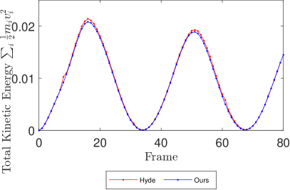
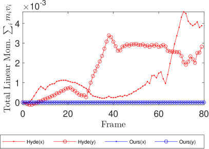
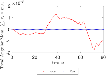
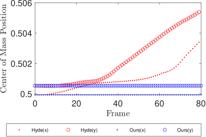
Figure 6. The present method (blue) conserves total mass, total linear and angular momentum, and center of mass, unlike Hyde et al. (2020) (red). Both methods are energy-dissipative.

6.2. Droplet Impact on Dry Surface

We demonstrate our method’s ability to handle highly dynamic simulations with a wide range of surface tension strengths. We simulated several spherical droplets with the same material parameters, each of which free falls from a fixed height and impacts a dry, frictionless, hydrophobic surface. The bulk modulus is 83333.33 and the gravitational acceleration is 9.8. The same grid resolution of $\Delta x=1/127$ was used for all the simulations, and the time step was restricted between $10^{-2}$ to $5\times 10^{-5}$ seconds by the CFL condition. With different surface tension coefficient $k^{\sigma}$, the droplet showed distinct behaviors upon impact, as shown in Figure 7.

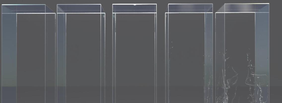
Figure 7. (Top) Spherical droplets with different surface tension coefficient free fall from the same height. In the top figure, from left to right, the surface tension coefficients are $k^{\sigma}=20,5,1,0.1,0.05$. (Middle Row) full rebound of the droplet (initial height: $3.5$ and $k^{\sigma}=15$). (Bottom Row) partial rebound of the droplet (initial height: $2.5$ and $k^{\sigma}=5$).

We also captured the partial rebound and the full rebound behaviors of the droplet after the impact. The middle and bottom rows of Figure 7 show the footage of a droplet with $k^{\sigma}=15$ dropped from a height of $3.5$ and a droplet with $k^{\sigma}=5$ dropped from a height of $2.5$, respectively. With a higher surface tension coefficient and a higher impact speed, the droplet is able to completely leave the surface after the impact. Our results qualitatively match the experiment outcomes from Rioboo et al. (2001).

6.3. Droplets on Ramps

As discussed in Section 3.6, our method allows for distinct $k^{\sigma}$ values at solid-liquid and liquid-air interfaces. Tuning the ratio between $k^{\sigma}$ at these interfaces allows simulating different levels of hydrophilicity/hydrophobicity. Figure 8 shows an example of several liquid drops with different $k^{\sigma}$ ratios falling on ramps of $5.5^{\circ}$ angle. The grid resolution was $\Delta x=1/63$, and the time step was restricted between $10^{-2}$ and $10^{-4}$ seconds by the CFL condition. Coulomb friction with a friction coefficient of $0.2$ was used for the ramp surface. When there is a larger difference between solid-liquid and liquid-air surface tension coefficients (i.e., a smaller $k^{\sigma}$ ratio), the liquid tends to drag more on the surface and undergo more separation and sticking. The leftmost example, with a $k^{\sigma}$ ratio of $0.05$, exhibits hydrophobic behavior.

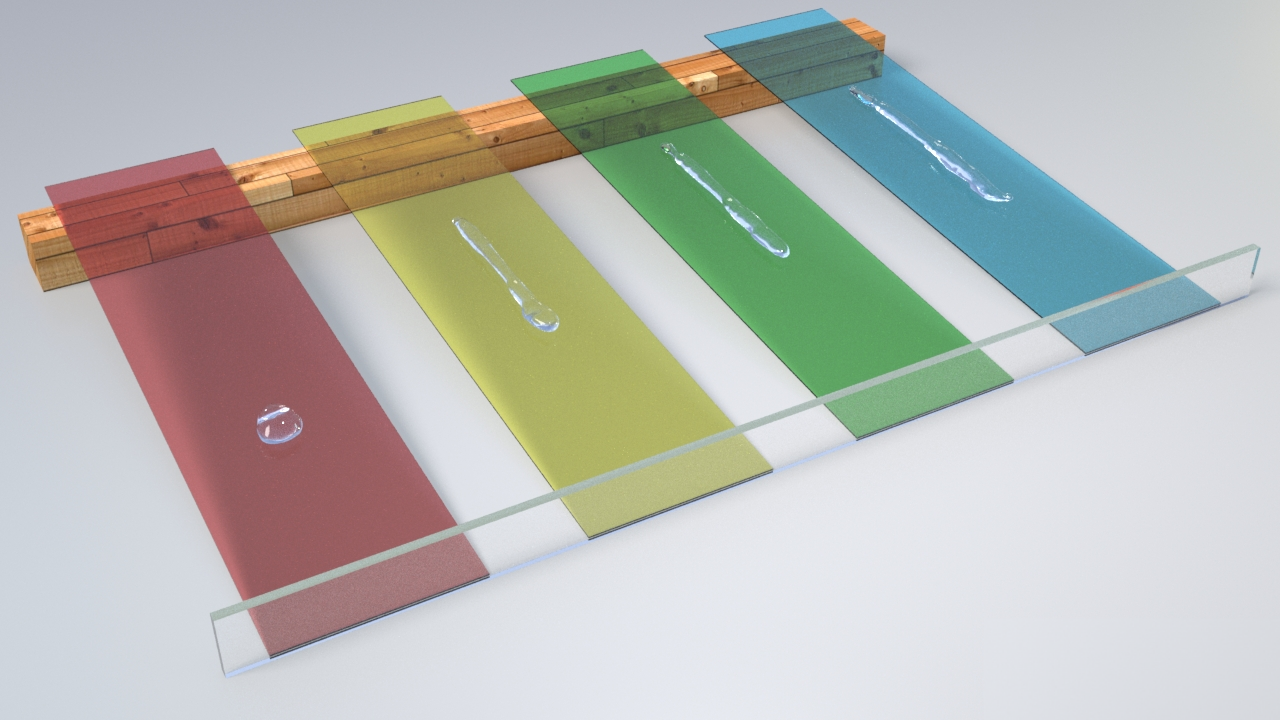
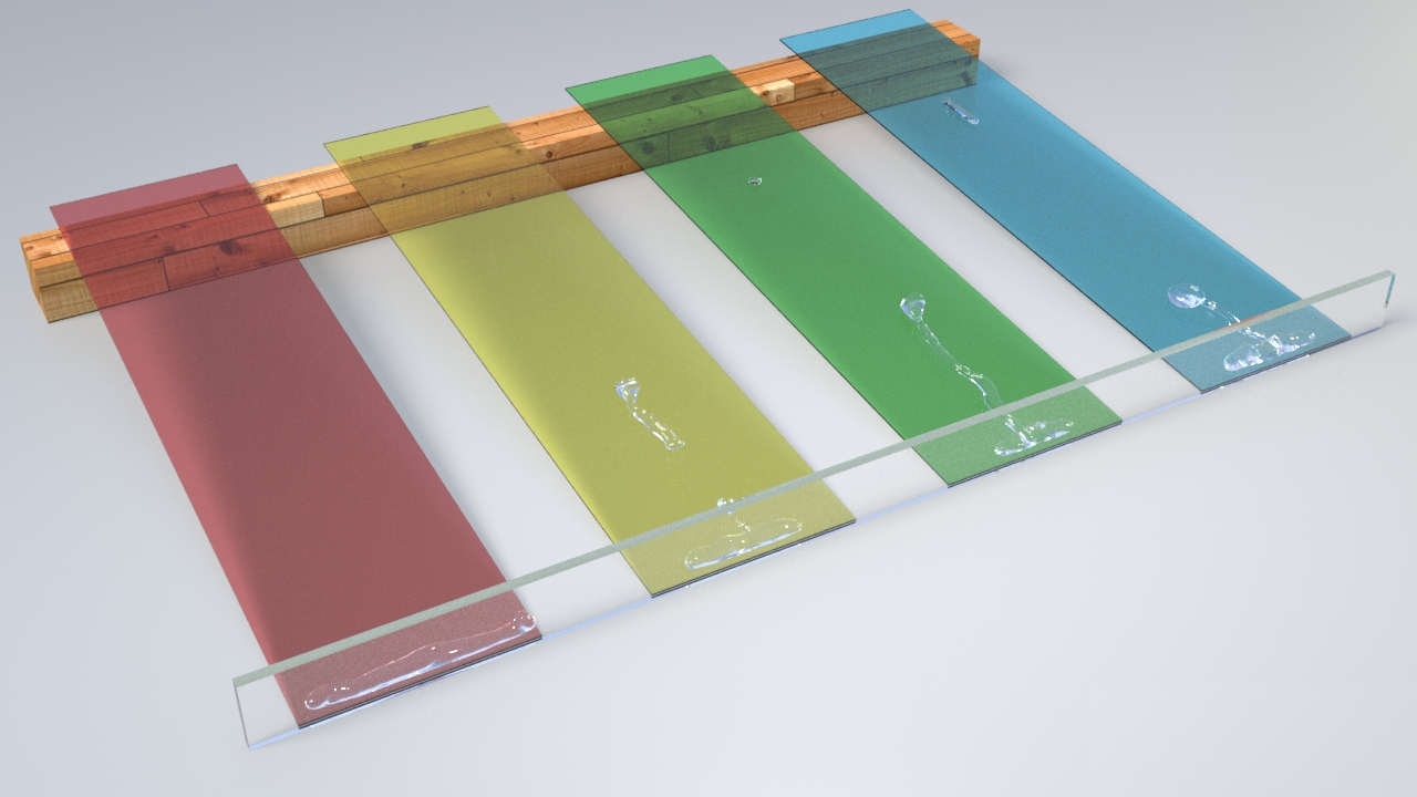
Figure 8. Liquid drops fall on a ramp with varying ratios between the solid-liquid and liquid-air surface tension coefficients. From left to right: ratios of $0.05$, $0.3$, $0.6$, $1.0$. (Top) Frame 60. (Bottom) Frame 100.

6.4. Lid-Driven Cavity

The two-dimensional lid-driven cavity is a classic example in the engineering literature of the Marangoni effect (Francois et al., 2006; Hopp-Hirschler et al., 2018). Inspired by works like these, we simulate a square unit domain and fill the domain with particles up to height $1-4\Delta x$ ($\Delta x=1/63$), which results in a free surface near the top of the domain. A linear temperature gradient from 1 on the left to 0 on the right is initialized on the particles. To achieve the Marangoni effect, the surface tension coefficient $k^{\sigma}$ is set to depend linearly on temperature: $k^{\sigma}=1-T_{p}$. $k^{\sigma}$ is clamped to be in $[0,1]$ to avoid artifacts due to numerical precision. Gravity is set to zero, dynamic viscosity is set to $1\text{\times}{10}^{-6}$ and implicit MPM is used with a maximum $\Delta t$ of $0.001$. Results are shown in Figure 9. We note that the center of the circulation drifts to the right over the course of the simulation due to uneven particle distribution resulting from the circulation of the particles; investigating particle reseeding strategies to stabilize the flow is interesting future work.

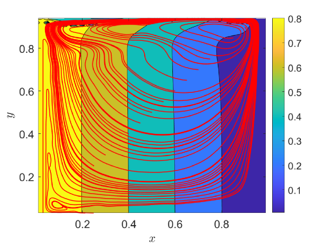
Figure 9. Frame 500 of a two-dimensional lid-driven cavity simulation. The simulation is initially stationary, but velocity streamlines (red) show the flow pattern characteristic of Marangoni convection that develops due to a temperature-dependent surface tension coefficient. The contour plot shows the evolving temperature field (initially a linear horizontal distribution).

6.5. Contact Angles

Figure 10 shows that our method enables simulation of various contact angles, emulating various degrees of hydrophobic or hydrophilic behavior as a droplet settles on a surface. We adjust the contact angles by assigning one surface tension coefficient, $k^{\sigma}_{LG}$, to the surface particles on the liquid-gas interface, and another one, $k^{\sigma}_{SL}$, to those on the solid-liquid interface. Following the Young equation (Equation (11)) and our assumption that $k^{\sigma}_{SG}$ is negligible, the contact angle is given by $\theta=\arccos\big(-k^{\sigma}_{SL}/k^{\sigma}_{LG}\big{missing})$. Note that the effect of gravity will result in contact angles slightly smaller than targeted. The grid resolution was set to $\Delta x=1/127$, and the time step restricted between $0.0333$ and $1\times 10^{-4}$. Each droplet is discretized using $230$k interior particles and $250$k surface particles. The bulk modulus of the fluid is $83333.33$, $k^{\sigma}_{LG}$ is set to $2$, and the dynamic viscosity is $0.075$.

Figure 10. As our droplets settle, we are able to obtain contact angles of approximately 45, 90, 135 and 180 degrees, using a $k^{\sigma}_{SL}/k^{\sigma}_{LG}$ ratio of $-\sqrt{2}/2$, $0$, $\sqrt{2}/2$ and $1$, respectively.

6.6. Soap Droplet in Water

We demonstrate a surface tension driven flow by simulating the soap reducing the surface tension of the water. We initialize a $1\times 0.05\times 1$ rectangular water pool and identify the particles in the middle of the top surface as liquid soap. Boundary particles associated with the water particles have higher surface tension than those associated with the soap particles. In order to visualize the effect of the surface tension driven flow, we randomly selected marker particles on the top surface of the pool. Due to the presence of the soap, the center of the pool has lower surface tension than the area near the edge of the container. Figure 11 shows footage of this process. A grid resolution of $\Delta x=1/127$ was used, and the time step was limited between $10^{-2}$ and $5\times 10^{-5}$ by the CFL number. The bulk modulus of water is set to be $16666.67$. The surface tension $k^{\sigma}$ for water is set to be $0.5$ and $k^{\sigma}$ for soap is $0.01$.

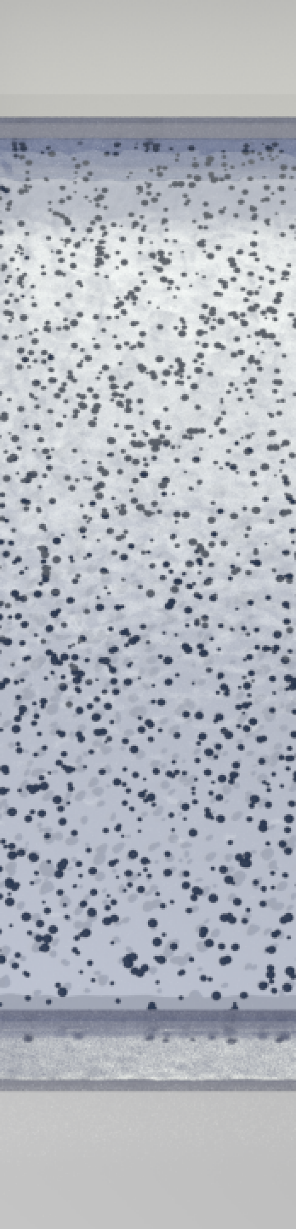
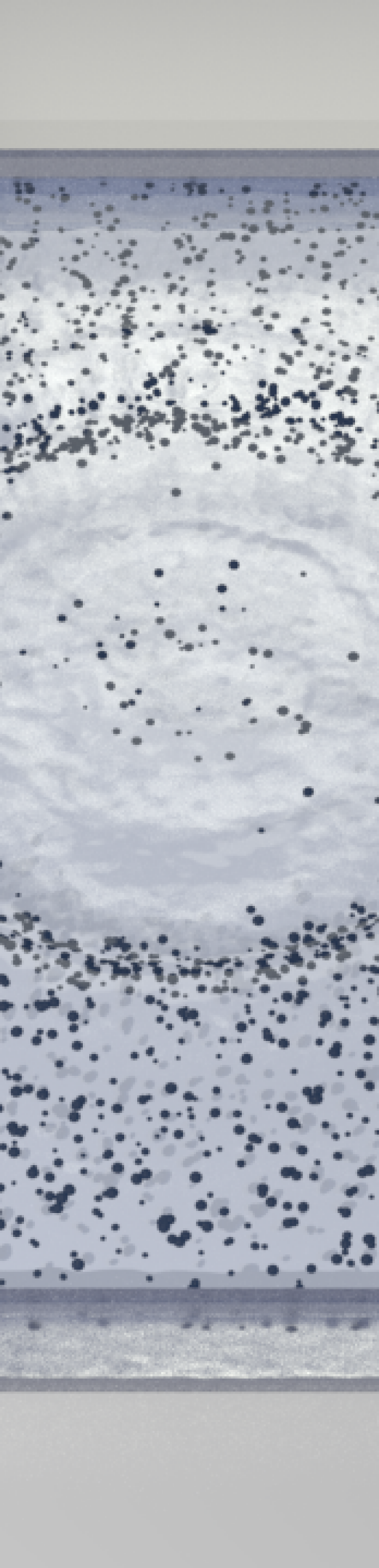
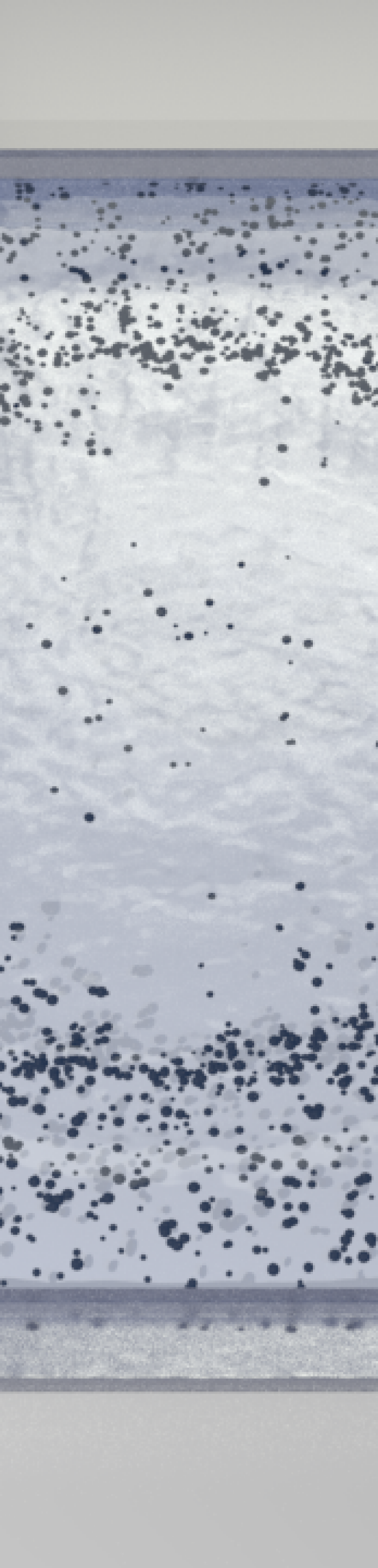
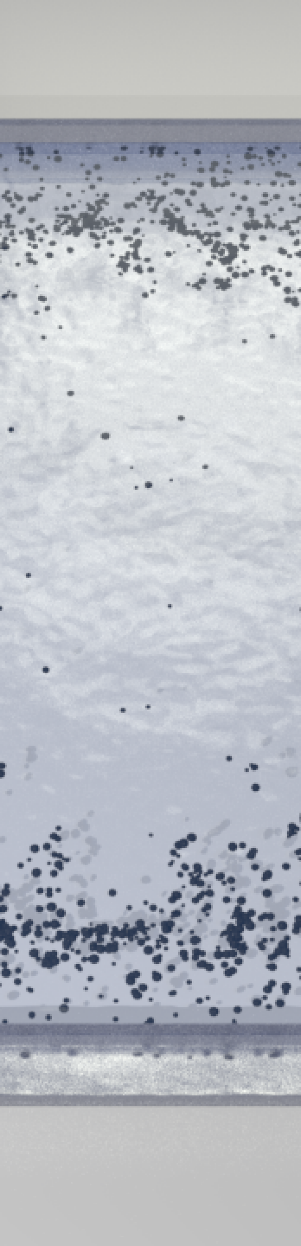
Figure 11. The soap in the center of the pool surface reduces the surface tension. The surface tension gradient drives the markers towards the walls of the container. Frames 0, 10, 20, 40 are shown in this footage.

6.7. Wine Glass

We consider an example of wine flowing on the surface of a pre-wetted glass. The glass is an ellipsoid centered at $(0.5,0.7,0.5)$ with characteristic dimensions $a=0.4$, $b=0.6$, and $c=0.4$. We initialize a thin band of particles with thickness of $2\Delta x$ on the surface of the wine glass and observe the formation of ridges and fingers as the particles settle toward the bulk fluid in the glass. The grid resolution is $\Delta x=1/127$ and a maximum allowable time step is $10^{-2}$ constrained by the CFL number. We set the surface tension coefficient on the liquid-gas interface is $k^{\sigma}_{LG}=0.05$ and the one on the solid-liquid interface is $k^{\sigma}_{SL}=0.015$. The piecewise constant surface tension gradient leads to a more prominent streaking behaviors of the liquid on the glass wall. The results are shown in Figure 12.

Figure 12. Wine is initialized in a glass with part of the interior pre-wetted. The falling wine forms tears and ridges, and the tears eventually connect with the bulk fluid. Frames 30 and 90 are shown.

6.8. Candles

We simulate several scenarios with wax candles. In these examples, wax melts due to a heat source (candle flame) and resolidifies when it flows away from the flame. Ambient temperature $\hat{T}$ is taken to be $298\text{K}$, and the melting point is $303\text{K}$. Thermal diffusivity $K$ is taken to be $0.1$, and specific heat capacity $c_{p}$ is set to $1$. No internal heat source is used ($H=0$); instead, heating and cooling are applied only via the boundary conditions.

To simulate the candle wicks, we manually construct and sample points on cubic splines. As the simulation progresses, we delete particles from the wick that are too far above the highest ($y$-direction) liquid particle within a neighborhood of the wick. The flames are created by running a separate FLIP simulation as a postprocess and anchoring the result to the exposed portion of each wick. We rendered these scenes using Arnold (Georgiev et al., 2018) and postprocessed the renders using the NVIDIA OptiX denoiser (based on Chaitanya et al. (2017)).

We consider the effect of varying $k^{\sigma}$ on the overall behavior of the flow. Figure 13 compares $k^{\sigma}$ values of $0.05$, $0.1$, $0.2$, and $0.4$. In these examples, a grid resolution of $\Delta x=1/127$ was used, along with boundary condition parameters $h=0.5$ and $b=50$. The figure demonstrates that as surface tension increases, the molten wax spreads significantly less. As the wax cools and resolidifies, visually interesting layering behavior is observed.

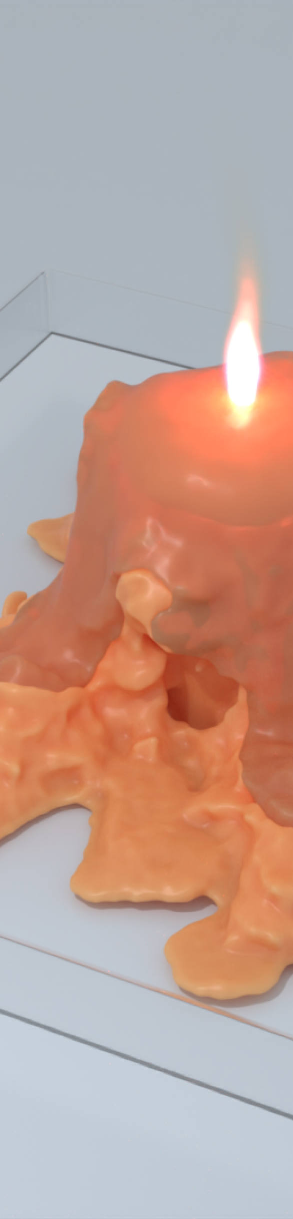
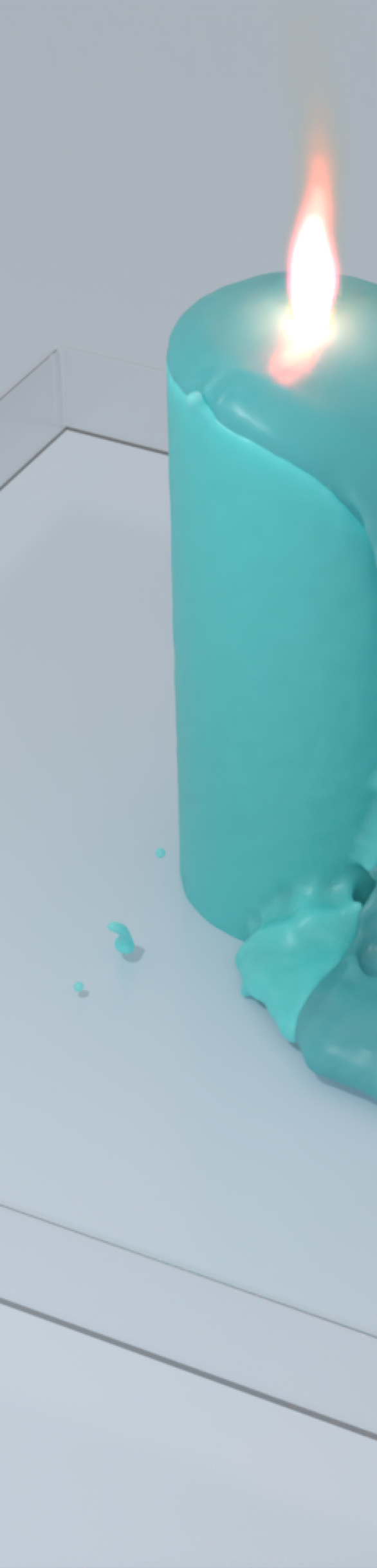
Figure 13. Various $k^{\sigma}$ values ($0.05$, $0.1$, $0.2$, $0.4$) are simulated in the case of a melting candle. Frame 1202 is shown.

Figure 14 shows an example of several candle letters melting in a container. Wicks follow generally curved paths inside the letters. Melt pools from the different letters seamlessly interact. This simulation used a surface tension coefficient $k^{\sigma}=0.05$, $h=2.5$, $b=100$, dynamic viscosity of $0.01$, $\Delta x=1/127$, and a bulk modulus of $83333.33$ for liquid and solid phases.

Figure 14. Letter-shaped candles melt inside a container. (Top) Frame 1, before flames are lit. (Middle) Frame 60, in the middle of melting. (Bottom) Frame 200, as flames are extinguished and wax pools resolidify.

6.9. Droplet with Marangoni Effect

We simulated a liquid metal droplet that moves under the Marangoni effect, i.e. due to a temperature-induced surface tension gradient. The droplet first falls to the ground and spreads on the dry surface. We then turn on the heating while the droplet is still spreading; only one side of the droplet is subjected to heating. At its original temperature, the surface tension coefficient $k^{\sigma}$ of the droplet is $0.5$. As the temperature increase, $k^{\sigma}$ increases linearly with the temperature. When the change in temperature is greater than $50K$, the surface tension coefficient reaches its maximum value of $5$. Since the hotter side of the droplet has higher surface tension, the stronger surface tension drives the particles to flow to the colder side as shown in Figure 15. This surface tension gradient results in an interesting self-propelled behavior of the liquid metal droplet. A domain of size $2\times 1\times 1$ with a grid resolution of $\Delta x=1/127$ is used for this example. The time step is restricted between $10^{-2}$ to $5\times 10^{-5}$ seconds by the CFL condition. The bulk modulus of the liquid is $83333.33$. $h=0.1$ and $b=50$ are used for the thermal boundary conditions.

Figure 15. A liquid metal droplet subjected to heating on one side. The surface tension coefficient increases as the temperature increases. (Top) the liquid metal at frame 45 and frame 130. (Bottom) the particle view of temperature distribution at frame 45 and frame 130. The red color indicates higher temperature.

6.10. Performance

Table 1 shows average per-timestep runtime details for several of our examples. For this table, all experiments were run on a workstation equipped with 128GB RAM and with dual Intel^® Xeon^® E5-2687W v4 CPUs at 3.00Ghz.

Table 1. Performance measurements for one time step of several of our examples, broken down by (1) generating surface and balance particles, (2) transferring MPM particle quantities to the background grid and implicit grid update, and (3) transferring background grid quantities to MPM particles, merging surface, balance and MPM particles, and updating MPM particle states. Note that the merging time does not exceed $3.5\%$ of (3). All times are in milliseconds.

Example	# Cells	# Int. Part.	# Surf. Part.	Sampling	Part.$\rightarrow$Grid	Grid$\rightarrow$Part.
Droplet Impact ($k^{\sigma}=5$)	2M	794K	100K	2224	7705	2360
Droplets on Ramps ($k^{\sigma}_{SL}/k^{\sigma}_{LG}=0.05$)	1.5M	70K	100K	258	1147	287
Contact Angles ($k^{\sigma}_{SL}/k^{\sigma}_{LG}=0$)	256K	230K	250K	492	3715	571
Soap Droplet in Water	1M	4M	200K	2166	32099	3205
Wine glass	2M	1.6M	500K	1549	11268	1172
Candle ($k^{\sigma}=0.1$)	2M	618K	50K	1420	27500	1662
Candle Letters	256K	3.1M	100K	4601	170048	2739
Droplet with Marangoni Effect	4.1M	235K	200K	29991	8812	3244

7. Discussion and Future Work

Our method allows for simulation of surface tension energies with spatial gradients, including those driven by variation in temperature. Our MPM approach to the problem resolves many interesting characteristic phenomena associated with these variations. However, while we provide for perfect conservation of linear and angular momentum, our approach to the thermal transfers is not perfectly conservative. Developing a thermally conservative transfer strategy is interesting future work. Also, although we simulate tears of wine on the walls of a glass, we did not simulate the effect of alcohol evaporation on the surface energy variation. Adding in a mixture model as in (Ding et al., 2019) would be interesting future work. Lastly, although our approach was designed for MPM, SPH is more commonly used for simulation of liquids. However, SPH and MPM have many similarities as recently shown by the work of Gissler et al. (Gissler et al., 2020b) and it would be interesting future work to generalize our approach to SPH.

References

- (1)
- Adamson and Gast (1967) A. Adamson and A. Gast. 1967. Physical chemistry of surfaces. Vol. 150. Interscience Publishers New York.
- Ando et al. (2012) R. Ando, N. Thurey, and R. Tsuruno. 2012. Preserving Fluid Sheets with Adaptively Sampled Anisotropic Particles. IEEE Trans Vis Comp Graph 18, 8 (Aug. 2012), 1202–1214.
- Annonymous (2021) Annonymous. 2021. Supplementary Technical Document. Technical Report.
- Azencot et al. (2015) O. Azencot, O. Vantzos, M. Wardetzky, M. Rumpf, and M. Ben-Chen. 2015. Functional thin films on surfaces. In Proc 14th ACM SIGGRAPH/Eurograph Symp Comp Anim. 137–146.
- Belytschko et al. (2013) T. Belytschko, W. Liu, B. Moran, and K. Elkhodary. 2013. Nonlinear finite elements for continua and structures. John Wiley and sons.
- Brackbill et al. (1992) J. Brackbill, D. Kothe, and C. Zemach. 1992. A continuum method for modeling surface tension. J Comp Phys 100, 2 (1992), 335–354.
- Buscaglia and Ausas (2011) G. Buscaglia and R. Ausas. 2011. Variational formulations for surface tension, capillarity and wetting. Comp Meth App Mech Eng 200, 45-46 (2011), 3011–3025.
- Cassie and Baxter (1944) A.B.D. Cassie and S. Baxter. 1944. Wettability of porous surfaces. Transactions of the Faraday society 40 (1944), 546–551.
- Chaitanya et al. (2017) C. R. A. Chaitanya, A. S. Kaplanyan, C. Schied, M. Salvi, A. Lefohn, D. Nowrouzezahrai, and T. Aila. 2017. Interactive reconstruction of Monte Carlo image sequences using a recurrent denoising autoencoder. ACM Trans Graph 36, 4 (2017), 1–12.
- Chen et al. (2020) Y.-L. Chen, J. Meier, B. Solenthaler, and V.C. Azevedo. 2020. An Extended Cut-Cell Method for Sub-Grid Liquids Tracking with Surface Tension. ACM Trans Graph 39, 6, Article 169 (Nov. 2020), 13 pages. https://doi.org/10.1145/3414685.3417859
- Chernyaev (1995) E. Chernyaev. 1995. Marching cubes 33: Construction of topologically correct isosurfaces. Technical Report.
- Clausen et al. (2013) P. Clausen, M. Wicke, J. R. Shewchuk, and J. F. O’brien. 2013. Simulating liquids and solid-liquid interactions with Lagrangian meshes. ACM Transactions on Graphics (TOG) 32, 2 (2013), 17.
- Corsini et al. (2012) M. Corsini, P. Cignoni, and R. Scopigno. 2012. Efficient and Flexible Sampling with Blue Noise Properties of Triangular Meshes. IEEE Trans Vis Comp Graph 18, 6 (2012), 914–924. https://doi.org/10.1109/TVCG.2012.34
- Da et al. (2015) F. Da, C. Batty, C. Wojtan, and E. Grinspun. 2015. Double bubbles sans toil and trouble: discrete circulation-preserving vortex sheets for soap films and foams. ACM Trans Graph (SIGGRAPH 2015) (2015).
- Da et al. (2016) F. Da, D. Hahn, C. Batty, C. Wojtan, and E. Grinspun. 2016. Surface-only liquids. ACM Trans Graph (TOG) 35, 4 (2016), 1–12.
- Daviet and Bertails-Descoubes (2016) G. Daviet and F. Bertails-Descoubes. 2016. A Semi-implicit Material Point Method for the Continuum Simulation of Granular Materials. ACM Trans Graph 35, 4 (2016), 102:1–102:13.
- de Langavant et al. (2017) C. C. de Langavant, A. Guittet, M. Theillard, F. Temprano-Coleto, and F. Gibou. 2017. Level-set simulations of soluble surfactant driven flows. J Comp Phys 348 (2017), 271–297.
- de Vaucorbeil et al. (2020) A. de Vaucorbeil, V. P. Nguyen, S. Sinaie, and J. Y. Wu. 2020. Chapter Two - Material point method after 25 years: Theory, implementation, and applications. Advances in Applied Mechanics, Vol. 53. Elsevier, 185 – 398. https://doi.org/10.1016/bs.aams.2019.11.001
- Ding et al. (2019) M. Ding, X. Han, S. Wang, T. Gast, and J. Teran. 2019. A thermomechanical material point method for baking and cooking. ACM Trans Graph 38, 6 (2019), 192.
- Dukler et al. (2020) Y. Dukler, H. Ji, C. Falcon, and A. L Bertozzi. 2020. Theory for undercompressive shocks in tears of wine. Phys Rev Fluids 5, 3 (2020), 034002.
- Edwards and Bridson (2012) E. Edwards and R. Bridson. 2012. A high-order accurate Particle-In-Cell method. Int J Numer Meth Eng 90 (2012), 1073–1088.
- Fang et al. (2019) Y. Fang, M. Li, Ming Gao, and Chenfanfu Jiang. 2019. Silly rubber: an implicit material point method for simulating non-equilibrated viscoelastic and elastoplastic solids. ACM Trans Graph 38, 4 (2019), 1–13.
- Farahi et al. (2004) R. Farahi, A. Passian, T. Ferrell, and T. Thundat. 2004. Microfluidic manipulation via Marangoni forces. Applied Phys Let 85, 18 (2004), 4237–4239.
- Fei et al. (2018) Y. Fei, C. Batty, E. Grinspun, and C. Zheng. 2018. A multi-scale model for simulating liquid-fabric interactions. ACM Trans Graph 37, 4 (2018), 51:1–51:16. https://doi.org/10.1145/3197517.3201392
- Fei et al. (2017) Y. Fei, H. Maia, C. Batty, C. Zheng, and E. Grinspun. 2017. A multi-scale model for simulating liquid-hair interactions. ACM Trans. Graph. 36, 4 (2017), 56:1–56:17. https://doi.org/10.1145/3072959.3073630
- Francois et al. (2006) M. M. Francois, J. M. Sicilian, and D. B. Kothe. 2006. Modeling of thermocapillary forces within a volume tracking algorithm. In Modeling of Casting, Welding and Advanced Solidification Processes–XI (Opio, France). 935–942.
- Fu et al. (2017) C. Fu, Q. Guo, T. Gast, C. Jiang, and J. Teran. 2017. A Polynomial Particle-in-cell Method. ACM Trans Graph 36, 6 (Nov. 2017), 222:1–222:12.
- Gao et al. (2017b) M. Gao, A. Tampubolon, C. Jiang, and E. Sifakis. 2017b. An adaptive generalized interpolation material point method for simulating elastoplastic materials. ACM Trans Graph 36, 6 (2017), 223:1–223:12. https://doi.org/10.1145/3130800.3130879
- Gao et al. (2017a) Y. Gao, S. Li, L. Yang, H. Qin, and A. Hao. 2017a. An efficient heat-based model for solid-liquid-gas phase transition and dynamic interaction. Graphical Models 94 (2017), 14 – 24. https://doi.org/10.1016/j.gmod.2017.09.001
- Georgiev et al. (2018) I. Georgiev, T. Ize, M. Farnsworth, R. Montoya-Vozmediano, A. King, B. Van Lommel, A. Jimenez, O. Anson, S. Ogaki, E. Johnston, A. Herubel, D. Russell, F. Servant, and M. Fajardo. 2018. Arnold: A brute-force production path tracer. ACM Transactions on Graphics (TOG) 37, 3 (2018), 1–12.
- Gissler et al. (2020a) C. Gissler, A. Henne, S. Band, A. Peer, and M. Teschner. 2020a. An Implicit Compressible SPH Solver for Snow Simulation. ACM Trans Graph 39, 4, Article 36 (July 2020), 16 pages. https://doi.org/10.1145/3386569.3392431
- Gissler et al. (2020b) C. Gissler, A. Henne, S. Band, A. Peer, and M. Teschner. 2020b. An implicit compressible SPH solver for snow simulation. ACM Trans Graph (TOG) 39, 4 (2020), 36–1.
- Gonzalez and Stuart (2008) O. Gonzalez and A. Stuart. 2008. A first course in continuum mechanics. Cambridge University Press.
- Gu and Yang (2016) Y. Gu and Y.-H. Yang. 2016. Physics Based Boiling Bubble Simulation. In SIGGRAPH ASIA 2016 Technical Briefs (Macau) (SA ’16). Association for Computing Machinery, New York, NY, USA, Article 5, 4 pages. https://doi.org/10.1145/3005358.3005385
- Guo et al. (2018) Q. Guo, X. Han, C. Fu, T. Gast, R. Tamstorf, and J. Teran. 2018. A material point method for thin shells with frictional contact. ACM Trans Graph 37, 4 (2018), 147. https://doi.org/10.1145/3197517.3201346
- Harlow and Welch (1965) F. Harlow and E. Welch. 1965. Numerical calculation of time-dependent viscous incompressible flow of fluid with free surface. Phys Fl 8, 12 (1965), 2182–2189.
- Hochstetter and Kolb (2017) H. Hochstetter and A. Kolb. 2017. Evaporation and Condensation of SPH-Based Fluids. In Proc ACM SIGGRAPH/Eurographics Symp Comp Anim (Los Angeles, California) (SCA ’17). Association for Computing Machinery, New York, NY, USA, Article 3, 9 pages. https://doi.org/10.1145/3099564.3099580
- Hopp-Hirschler et al. (2018) M. Hopp-Hirschler, M. S. Shadloo, and U. Nieken. 2018. A Smoothed Particle Hydrodynamics approach for thermo-capillary flows. Comp Fluids 176 (2018), 1 – 19. https://doi.org/10.1016/j.compfluid.2018.09.010
- Hu and Eberhard (2017) H. Hu and P. Eberhard. 2017. Thermomechanically coupled conduction mode laser welding simulations using smoothed particle hydrodynamics. Comp Part Mech 4 (Oct 2017), 473–486. Issue 4. https://doi.org/10.1007/s40571-016-0140-5
- Huang et al. (2020) W. Huang, J. Iseringhausen, T. Kneiphof, Z. Qu, C. Jiang, and M.B. Hullin. 2020. Chemomechanical Simulation of Soap Film Flow on Spherical Bubbles. ACM Trans Graph 39, 4, Article 41 (July 2020), 14 pages. https://doi.org/10.1145/3386569.3392094
- Hyde et al. (2020) D.A.B. Hyde, S.W. Gagniere, A. Marquez-Razon, and J. Teran. 2020. An Implicit Updated Lagrangian Formulation for Liquids with Large Surface Energy. ACM Trans Graph 39, 6, Article 183 (Nov. 2020), 13 pages. https://doi.org/10.1145/3414685.3417845
- Irving et al. (2004) G. Irving, J. Teran, and R. Fedkiw. 2004. Invertible Finite Elements for Robust Simulation of Large Deformation. In Proc ACM SIGGRAPH/Eurograph Symp Comp Anim. 131–140.
- Ishida et al. (2020) S. Ishida, P. Synak, F. Narita, T. Hachisuka, and C. Wojtan. 2020. A Model for Soap Film Dynamics with Evolving Thickness. ACM Trans Graph 39, 4, Article 31 (July 2020), 11 pages. https://doi.org/10.1145/3386569.3392405
- Jiang et al. (2017) C. Jiang, T. Gast, and J. Teran. 2017. Anisotropic elastoplasticity for cloth, knit and hair frictional contact. ACM Trans Graph 36, 4 (2017), 152.
- Jiang et al. (2015) C. Jiang, C. Schroeder, A. Selle, J. Teran, and A. Stomakhin. 2015. The Affine Particle-In-Cell Method. ACM Trans Graph 34, 4 (2015), 51:1–51:10.
- Jiang et al. (2016) C. Jiang, C. Schroeder, J. Teran, A. Stomakhin, and A. Selle. 2016. The Material Point Method for Simulating Continuum Materials. In ACM SIGGRAPH 2016 Course. 24:1–24:52.
- Johnson Jr. and Dettre (1964) R. E. Johnson Jr. and R. H. Dettre. 1964. Contact angle hysteresis. III. Study of an idealized heterogeneous surface. J Phys Chem 68, 7 (1964), 1744–1750.
- Klár et al. (2016) G. Klár, T. Gast, A. Pradhana, C. Fu, C. Schroeder, C. Jiang, and J. Teran. 2016. Drucker-prager Elastoplasticity for Sand Animation. ACM Trans Graph 35, 4 (2016), 103:1–103:12.
- Langbein (2002) D. Langbein. 2002. Capillary surfaces: shape – stability – dynamics, in particular under weightlessness. Vol. 178. Springer Science & Business Media.
- Lenaerts and Dutré (2009) T. Lenaerts and P. Dutré. 2009. An architecture for unified SPH simulations. CW Reports (2009).
- Li et al. (2020) W. Li, D. Liu, M. Desbrun, J. Huang, and X. Liu. 2020. Kinetic-based Multiphase Flow Simulation. IEEE Trans Vis Comp Graph (2020).
- Losasso et al. (2008) F. Losasso, J. Talton, N. Kwatra, and R. Fedkiw. 2008. Two-Way Coupled SPH and Particle Level Set Fluid Simulation. IEEE Trans Visu Comp Graph 14, 4 (2008), 797–804.
- Maeshima et al. (2020) T. Maeshima, Y. Kim, and T. I. Zohdi. 2020. Particle-scale numerical modeling of thermo-mechanical phenomena for additive manufacturing using the material point method. Computational Particle Mechanics (2020). https://doi.org/10.1007/s40571-020-00358-x
- Monaghan (1992) J. Monaghan. 1992. Smoothed particle hydrodynamics. Ann Rev Astron Astroph 30, 1 (1992), 543–574.
- Narain et al. (2010) R. Narain, A. Golas, and M. Lin. 2010. Free-flowing granular materials with two-way solid coupling. ACM Trans Graph 29, 6 (2010), 173:1–173:10.
- Nas and Tryggvason (2003) S. Nas and G. Tryggvason. 2003. Thermocapillary interaction of two bubbles or drops. Int J Multiphase Flow 29, 7 (2003), 1117–1135. https://doi.org/10.1016/S0301-9322(03)00084-3
- Osada et al. (2002) R. Osada, T. Funkhouser, B. Chazelle, and D. Dobkin. 2002. Shape Distributions. ACM Trans. Graph. 21, 4 (Oct. 2002), 807–832. https://doi.org/10.1145/571647.571648
- Paiva et al. (2009) A. Paiva, F. Petronetto, T. Lewiner, and G. Tavares. 2009. Particle-based viscoplastic fluid/solid simulation. Computer-Aided Design 41, 4 (2009), 306–314.
- Pauly et al. (2005) M. Pauly, R. Keiser, B. Adams, P. Dutré, M. Gross, and L. Guibas. 2005. Meshless animation of fracturing solids. ACM Trans Graph 24, 3 (2005), 957–964. https://doi.org/10.1145/1073204.1073296
- Pirk et al. (2017) S. Pirk, M. Jarz\kabek, T. Hädrich, D.L. Michels, and W. Palubicki. 2017. Interactive Wood Combustion for Botanical Tree Models. 36, 6, Article 197 (Nov. 2017), 12 pages. https://doi.org/10.1145/3130800.3130814
- Ram et al. (2015) D. Ram, T. Gast, C. Jiang, C. Schroeder, A. Stomakhin, J. Teran, and P. Kavehpour. 2015. A material point method for viscoelastic fluids, foams and sponges. In Proc ACM SIGGRAPH/Eurograph Symp Comp Anim. 157–163.
- Rioboo et al. (2001) R. Rioboo, C. Tropea, and M. Marengo. 2001. Outcomes from a Drop Impact on Solid Surfaces. Atomization and Sprays 11, 2 (2001).
- Russell (2018) M. A. Russell. 2018. A Smoothed Particle Hydrodynamics Model for the Simulation of Laser Fusion Additive Manufacturing Processes. Ph.D. Dissertation. UC Berkeley.
- Schreck and Wojtan (2020) C. Schreck and C. Wojtan. 2020. A practical method for animating anisotropic elastoplastic materials. Computer Graphics Forum - Eurographics 2020 39, 2 (2020).
- Scriven and Sternling (1960) L. Scriven and C. Sternling. 1960. The marangoni effects. Nature 187, 4733 (1960), 186–188.
- Stomakhin et al. (2012) A. Stomakhin, R. Howes, C. Schroeder, and J. Teran. 2012. Energetically consistent invertible elasticity. In Proc Symp Comp Anim. 25–32.
- Stomakhin et al. (2013) A. Stomakhin, C. Schroeder, L. Chai, J. Teran, and A. Selle. 2013. A Material Point Method for snow simulation. ACM Trans Graph 32, 4 (2013), 102:1–102:10.
- Stomakhin et al. (2014) A. Stomakhin, C. Schroeder, C. Jiang, L. Chai, J. Teran, and A. Selle. 2014. Augmented MPM for phase-change and varied materials. ACM Trans Graph 33, 4 (2014), 138:1–138:11.
- Sulsky et al. (1994) D. Sulsky, Z. Chen, and H. Schreyer. 1994. A particle method for history-dependent materials. Comp Meth App Mech Eng 118, 1 (1994), 179–196.
- Sussman and Ohta (2009) M. Sussman and M. Ohta. 2009. A stable and efficient method for treating surface tension in incompressible two-phase flow. SIAM J Sci Comp 31, 4 (2009), 2447–2471.
- Tartakovsky and Meakin (2005) A. Tartakovsky and P. Meakin. 2005. Modeling of surface tension and contact angles with smoothed particle hydrodynamics. Phys Rev E 72 (Aug 2005), 026301. Issue 2. https://doi.org/10.1103/PhysRevE.72.026301
- Terzopoulos et al. (1991) D. Terzopoulos, J. Platt, and K. Fleischer. 1991. Heating and melting deformable models. The Journal of Visualization and Computer Animation 2, 2 (1991), 68–73.
- Thomson (1855) J. Thomson. 1855. XLII. On certain curious motions observable at the surfaces of wine and other alcoholic liquors. London, Edinburgh, and Dublin Phil Mag J Sci 10, 67 (1855), 330–333.
- Thürey et al. (2010) N. Thürey, C. Wojtan, M. Gross, and G. Turk. 2010. A multiscale approach to mesh-based surface tension flows. ACM Trans Graph (TOG) 29, 4 (2010), 1–10.
- Tong and Browne (2014) M. Tong and D. J. Browne. 2014. An incompressible multi-phase smoothed particle hydrodynamics (SPH) method for modelling thermocapillary flow. Int J Heat Mass Transfer 73 (2014), 284 – 292. https://doi.org/10.1016/j.ijheatmasstransfer.2014.01.064
- Venerus and Simavilla (2015) D. C. Venerus and D. N. Simavilla. 2015. Tears of wine: New insights on an old phenomenon. Scientific reports 5 (2015), 16162.
- Wang et al. (2012) C. Wang, Q. Zhang, H. Xiao, and Q. Shen. 2012. Simulation of multiple fluids with solid-liquid phase transition. Comp Anim Virtual Worlds 23, 3-4 (2012), 279–289. https://doi.org/10.1002/cav.1457 arXiv:https://onlinelibrary.wiley.com/doi/pdf/10.1002/cav.1457
- Wang et al. (2020a) H. Wang, Y. Jin, A. Luo, X. Yang, and B. Zhu. 2020a. Codimensional Surface Tension Flow Using Moving-Least-Squares Particles. ACM Trans Graph 39, 4, Article 42 (July 2020), 16 pages. https://doi.org/10.1145/3386569.3392487
- Wang et al. (2007) H. Wang, G. Miller, and G. Turk. 2007. Solving General Shallow Wave Equations on Surfaces (SCA ’07). Eurographics Association, Goslar, DEU, 229–238.
- Wang et al. (2005) H. Wang, P. J. Mucha, and G. Turk. 2005. Water Drops on Surfaces. ACM Tran. Graph 24, 3 (July 2005), 921–929. https://doi.org/10.1145/1073204.1073284
- Wang et al. (2019) S. Wang, M. Ding, T. Gast, L. Zhu, S. Gagniere, C. Jiang, and J. Teran. 2019. Simulation and Visualization of Ductile Fracture with the Material Point Method. Proceedings of the ACM on Computer Graphics and Interactive Techniques 2, 2, 18.
- Wang et al. (2020b) X. Wang, M. Li, Y. Fang, X. Zhang, M. Gao, M. Tang, D. Kaufman, and C. Jiang. 2020b. Hierarchical optimization time integration for CFL-rate MPM stepping. ACM Trans Graph (TOG) 39, 3 (2020), 1–16.
- Wang et al. (2020c) X. Wang, Y. Qiu, S.R. Slattery, Y. Fang, M. Li, S.-C. Zhu, Y. Zhu, M. Tang, D. Manocha, and C. Jiang. 2020c. A Massively Parallel and Scalable Multi-GPU Material Point Method. ACM Trans Graph 39, 4, Article 30 (July 2020), 15 pages. https://doi.org/10.1145/3386569.3392442
- Wojtan et al. (2010) C. Wojtan, N. Thürey, M. Gross, and G. Turk. 2010. Physics-inspired topology changes for thin fluid features. ACM Trans Graph 29, 4 (2010), 50:1–50:8. https://doi.org/10.1145/1778765.1778787
- Wolper et al. (2020) J. Wolper, Y. Chen, M. Li, Y. Fang, Z. Qu, J. Lu, M. Cheng, and C. Jiang. 2020. AnisoMPM: animating anisotropic damage mechanics. ACM Trans. Graph. 39, 4, Article 37 (2020).
- Wolper et al. (2019) J. Wolper, Y. Fang, M. Li, J. Lu, M. Gao, and C. Jiang. 2019. CD-MPM: continuum damage material point methods for dynamic fracture animation. ACM Trans. Graph. 38, 4, Article 119 (2019).
- Yang et al. (2016a) S. Yang, X. He, H. Wang, S. Li, G. Wang, E. Wu, and K. Zhou. 2016a. Enriching SPH simulation by approximate capillary waves. In Symp Comp Anim. 29–36.
- Yang et al. (2017) T. Yang, J. Chang, M. C. Lin, R. R. Martin, J. J. Zhang, and S.-M. Hu. 2017. A unified particle system framework for multi-phase, multi-material visual simulations. ACM Transactions on Graphics (TOG) 36, 6 (2017), 224.
- Yang et al. (2016b) T. Yang, M. C. Lin, R. R. Martin, J. Chang, and S.-M. Hu. 2016b. Versatile Interactions at Interfaces for SPH-Based Simulations (SCA ’16). Eurographics Association, Goslar, DEU, 57–66.
- Young (1805) T. Young. 1805. III. An essay on the cohesion of fluids. Phil Trans Royal Soc London 95 (1805), 65–87. https://doi.org/10.1098/rstl.1805.0005 arXiv:https://royalsocietypublishing.org/doi/pdf/10.1098/rstl.1805.0005
- Yue et al. (2015) Y. Yue, B. Smith, C. Batty, C. Zheng, and E. Grinspun. 2015. Continuum foam: a material point method for shear-dependent flows. ACM Trans Graph 34, 5 (2015), 160:1–160:20.
- Zhang et al. (2017) T. Zhang, J. Shi, C. Wang, H. Qin, and C. Li. 2017. Robust Gas Condensation Simulation with SPH based on Heat Transfer. In Pacific Graphics Short Papers, Jernej Barbic, Wen-Chieh Lin, and Olga Sorkine-Hornung (Eds.). The Eurographics Association, 27–32. https://doi.org/10.2312/pg.20171321
- Zheng et al. (2015) W. Zheng, B. Zhu, B. Kim, and R. Fedkiw. 2015. A new incompressibility discretization for a hybrid particle MAC grid representation with surface tension. J Comp Phys 280 (2015), 96–142.
- Zhu et al. (2014) B. Zhu, E. Quigley, M. Cong, J. Solomon, and R. Fedkiw. 2014. Codimensional surface tension flow on simplicial complexes. ACM Trans Graph (TOG) 33, 4 (2014), 1–11.