Multiple ground-state instabilities in the anisotropic quantum Rabi model

Abstract

In this work, the anisotropic variant of the quantum Rabi model with different coupling strengths of the rotating and counter-rotating wave terms is studied by the Bogoliubov operator approach. The anisotropy preserves the parity symmetry of the original model. We derive the corresponding $G$-function, which yields both the regular and exceptional eigenvalues. The exceptional eigenvalues correspond to the crossing points of two energy levels with different parities and are doubly degenerate. We find analytically that the ground-state and the first excited state can cross several times, indicating multiple first-order phase transitions as function of the coupling strength. These crossing points are related to manifest parity symmetry of the Hamiltonian, in contrast to the level crossings in the asymmetric quantum Rabi model which are caused by a hidden symmetry.

I Introduction

The Quantum Rabi model (QRM) describes a two-level system coupled to a single electromagnetic mode (an oscillator) via the dipole term Rabi , the simplest form of light-matter interaction. As such it has many applications in numerous fields ranging from quantum optics and quantum information science to condensed matter physics. In conventional (weak coupling) applications to quantum optics, the rotating-wave (RW) terms are kept and the counter-rotating-wave (CRW) terms are neglected Scully . This so-called rotating-wave approximation (RWA) is equivalent to the Jaynes-Cummings model Jaynes-Cummings , which is solvable in closed form.

Over the past decade, developments in circuit QED Wallraff ; Deppe have allowed to reach the ultra-strong coupling regime where the coupling between the superconducting qubit and the resonator can reach $10\%$ of the mode frequency $\omega$. In this ultrastrong-coupling regime, evidence for the breakdown of the RWA and the importance of CRW terms has been provided by measurements of transmission spectra Niemczyk ; exp . More recently, even the deep strong coupling region has been realized experimentally, where the coupling strength is of the same order as the mode frequency Yoshihara . In this regime, the RWA cannot even qualitatively describe the system Casanova . Although the spectrum of the full QRM is very easy to obtain numerically by working in a truncated bosonic Hilbert space, the exact analytical solution and with it qualitative statements about the spectrum are difficult to obtain compared to the super-integrable Jaynes-Cummings model. Analytical approximations have been obtained at different levels, such as the limit of small energy splitting $\Delta$ of the qubit ($\Delta/\omega<0.5$) and the deep strong coupling regime  $g/\omega\sim 1$ Casanova ; Hausinger ; Ashhab , weak and intermediate coupling ($g/\omega<0.4$) He , and also in the whole parameter range Feranchuk ; Irish ; zhengh . All these approximations, while numerically often satisfying, miss some qualitative features of the exact spectral graph like true level crossings and narrow avoided crossings.

An analytical solution based on the $\mathbb{Z}_{2}$-symmetry of the model and using the Bargmann representation of $L^{2}(\mathbb{R})$ introduced a transcendental function, called $G$-function in Braak , whose zeros yield the exact spectrum of the QRM. Shortly afterwards, it was found that the $G$-function can be written in terms of Heun functions, known from the theory of linear differential equations in the complex domain Zhong . The $G$-function has a characteristic pole structure, giving information about the form of the eigenstates and the distribution of the eigenvalues along the real axis Duan18 ; Braak19 . With its help, one may classify the eigenvalues as belonging either to the regular or to the exceptional spectrum, the former always non-degenerate, while the latter is comprised of a degnerate and a non-degenerate part Braak ; Wakayama . The $G$-function can be derived also in the more familiar Hilbert space $L^{2}(\mathbb{R})$, using the Bogoliubov operator approach, and thus in a physically more intuitive way Chen2012 .

The “anisotropic” generalization of the QRM where RW and CRW terms have different coupling strengths (AiQRM) has been studied for quite a long time, initially out of pure theoretical interest. It appeared first in the form of the anisotropic variant of the Dicke model Furuya . Recently, Goldstone and Higgs modes have been experimentally demonstrated in optical systems with only a few (artificial) atoms, which can be described by the anisotropic Dicke model with a small number of qubits yejw2013 . This experimental progress motivated theoretical studies of the anisotropic QRM (a single qubit) Fanheng ; Tomka . The AiQRM can also model a two-dimensional electron gas with Rashba ($\alpha_{R},$ corresponding to RW coupling) and Dresselhaus ($\alpha_{D},$ corresponding to CRW coupling) spin-orbit interactions, subject to a perpendicular magnetic field Erlingsson . The two types of couplings can be tuned by external electric and magnetic fields, allowing the exploration of the whole parameter space of the model. It can also be directly realized in both cavity QED Schiroa and circuit QED Wallraff . For example, Ref. Grimsmo proposes a realization of the AiQRM based on resonant Raman transitions in an atom interacting with a high finesse optical cavity mode. Very recently, it has been proposed that the AiQRM can also be realized in the dispersive regime via momentum states instead of electronic states Mivehvara .

The exact solution of the AiQRM has been obtained using the Bargmann representation Fanheng ; Tomka . The $G$-function was obtained by Xie et al. Fanheng , and both regular and exceptional eigenvalues have been studied. The isolated exact solutions at the level crossings (i.e. a part of the exceptional spectrum) were found by Tomka et al. Tomka . The surprising finding of Ref. Fanheng was that for certain parameter values the first excited state may form a degenerate doublet with the ground state and belongs thus to the exceptional spectrum, which can never happen in the isotropic QRM braak-fmi .

At this level crossing, the parity of the ground state changes sign and the system undergoes a first order quantum phase transition Fanheng . In the framework of the Bogoliubov operator approach, the anisotropic QRM has been solved by two of the present authors Duan2015 . The doubly degenerate exceptional solutions are explicitly given in Eq. (14) of Ref. Duan2015 as a methodical alternative to Ref. Tomka , where the problem was treated by a Bethe ansatz of Gaudin-Richardson type. Recently, it has been claimed that the quantum phase transition of the AiQRM is accompanied by the breaking of a hidden symmetry yingzj .

The AiQRM continues to be an interesting topic, because it connects continuously the Jaynes-Cummings model with the isotropic QRM. We revisit the AiQRM along the lines of Duan2015 and focus on the crossings of the first two energy levels in the spectral graph as function of increasing coupling strength.

The paper is organized as follows. In Sec. II, we construct the $G$-function using extended coherent states. In Sec. III, we analyze the exceptional spectrum, which contains all possible level degeneracies, with the help of the $G$-function. We discuss the crossings between the two lowest levels in Sec. IV, and we obtain their properties analytically. In this way, the ground state phase diagram of the AiQRM in the plane spanned by the coupling strength and the anisotropy parameter is obtained. We summarize our findings in Sec. V.

II Model and analytic solutions

The Hamiltonian of the anisotropic QRM reads Fanheng ; Tomka

$$H=\frac{1}{2}\Delta\sigma_{z}+\omega a^{\dagger}a+g_{1}\left(a^{\dagger}\sigma_{-}+a\sigma_{+}\right)+g_{2}\left(a^{\dagger}\sigma_{+}+a\sigma_{-}\right),$$ (1)

where $\Delta$ is qubit level splitting, $a^{\dagger}$ $\left(a\right)$ is the photonic creation (annihilation) operator of the single radiation mode with frequency $\omega$ (set to $1=\hbar=\omega$ in the following and the figures), $g_{1}\$and $g_{2}\$ are the RW and CRW coupling constants respectively, and $\sigma_{k}(k=x,y,z)$    are the Pauli matrices. Set $r=g_{2}/g_{1}\$as the anisotropic parameter and $g=g_{1}$ below.

The anisotropic QRM possesses the same $\mathbb{Z}_{2}$ symmetry as the isotropic one. The parity operator is defined as $\hat{\Pi}=\exp\left(i\pi\hat{N}\right)$, where $\hat{N}=a^{{\dagger}}a+\sigma_{+}\sigma_{-}$ with $\sigma_{\pm}=\left(\sigma_{x}\pm i\sigma_{y}\right)/2$ is the operator of the total excitation number. Note that while $\hat{N}$ is not conserved, the Hamiltonian (1) conserves its parity, ($\hat{N}\ \text{mod}\ 2$) and therefore $\hat{\Pi}$. The parity operator $\hat{\Pi}$ has two eigenvalues  $\Pi=\pm 1$, corresponding to even and odd parity of $\hat{N}$.

We proceed to derive the $G$-function of (1). Employing the following transformation

$$P=\frac{1}{\sqrt{2}}\left(\begin{array}[]{ll}\sqrt{r}&~{}1\\ -\sqrt{r}&\;1\end{array}\right),\;\;P^{-1}=\frac{1}{\sqrt{2}}\left(\begin{array}[]{ll}\;\frac{1}{\sqrt{r}}&~{}-\frac{1}{\sqrt{r}}\\ \;\;\;\;1&\;\;\;\;\;1\end{array}\right),$$ (2)

the Hamiltonian becomes

$$H_{1}=PHP^{-1}=\left(\begin{array}[]{ll}a^{\dagger}a+\beta\left(a+a^{\dagger}\right)+\left(\frac{\lambda_{+}}{\beta}-\beta\right)a^{\dagger}&\;\;\;\;-\frac{1}{2}\Delta-\frac{\lambda_{-}}{\beta}a^{\dagger}\\ \;\;\;\;-\frac{1}{2}\Delta+\frac{\lambda_{-}}{\beta}a^{\dagger}&\;a^{\dagger}a-\beta\left(a+a^{\dagger}\right)-\left(\frac{\lambda_{+}}{\beta}-\beta\right)a^{\dagger}\end{array}\right),$$ (3)

where $\lambda_{\pm}=g^{2}\left(1\pm r^{2}\right)/2$ and$\;\beta=g\sqrt{r}$.

We introduce two displaced bosonic operators with opposite displacements

$$A_{+}^{\dagger}=a^{\dagger}+\beta;\;\;A_{-}^{\dagger}=a^{\dagger}-\beta.$$ (4)

The bosonic number state in terms of the new photonic operators $A_{+}^{\dagger}$ and $A_{-}^{\dagger}$ are

$$\left|n\right\rangle_{A_{+}} = \frac{\left(A_{+}^{\dagger}\right)^{n}}{\sqrt{n!}}D(-\beta)\left|0\right\rangle$$

$$\left|n\right\rangle_{A_{-}} = \frac{\left(A_{-}^{\dagger}\right)^{n}}{\sqrt{n!}}D(\beta)\left|0\right\rangle,$$

where $D(\beta)=\exp\left(\beta a^{\dagger}-\beta a\right)$ is the unitary displacement operator, acting on the original vacuum state $\left|0\right\rangle$ ($a|0\rangle=0$). The states $\{\left|n\right\rangle_{A_{+}}\}_{n}$, respectively $\{\left|n\right\rangle_{A_{-}}\}_{n}$, form an orthonormal basis of the bosonic Hilbert space $L^{2}(\mathbb{R})$ and are called extended coherent states (ECS) chenqh . Note that the hermitian conjugated operators $A_{\pm}=(A^{\dagger}_{\pm})^{\dagger}$ annihilate the respective displaced vacua $|0\rangle_{A_{\pm}}=D(\mp\beta)|0\rangle$.

The Hamiltonian in terms of $A_{+}^{\dagger}$, $A_{+}$ reads

$$H_{1}=\left(\begin{array}[]{ll}A_{+}^{\dagger}A_{+}+\left(\lambda_{+}/\beta-\beta\right)A_{+}^{\dagger}-\lambda_{+}&\;\;\;\;\left(-\frac{1}{2}\Delta+\lambda_{-}\right)-\frac{\lambda_{-}}{\beta}A_{+}^{\dagger}\\ \;\;\;\;\left(-\frac{1}{2}\Delta-\lambda_{-}\right)+\frac{\lambda_{-}}{\beta}A_{+}^{\dagger}&\;A_{+}^{\dagger}A_{+}-\left(\beta+\lambda_{+}/\beta\right)A_{+}^{\dagger}-2\beta A_{+}+2\beta^{2}+\lambda_{+}\end{array}\right).$$ (5)

The wavefunction can be expressed as the following series expansion using these ECS

$$\left|A_{+}\right\rangle=\left(\begin{array}[]{c}\sum_{n=0}^{\infty}\sqrt{n!}e_{n}|n\rangle_{A_{+}}\\ \sum_{n=0}^{\infty}\sqrt{n!}f_{n}|n\rangle_{A_{+}}\end{array}\right).$$ (6)

Multiplying the time-independent Schrödinger equation with the bra-vector $\;{}_{A_{+}}\left\langle m\right|\;$ from the left yields a recurrence relation for the coefficients

$$e_{m} = \frac{\left(\beta-\frac{\lambda_{+}}{\beta}\right)e_{m-1}+\left(\frac{1}{2}\Delta-\lambda_{-}\right)f_{m}+\frac{\lambda_{-}}{\beta}f_{m-1}}{m-x},$$ (7)

$$f_{m} = \frac{\;\left(-\frac{1}{2}\Delta-\lambda_{-}\right)e_{m-1}+\frac{\lambda_{-}}{\beta}e_{m-2}+\left(m-1+2\beta^{2}+2\lambda_{+}-x\right)f_{m-1}-\left(\beta+\lambda_{+}/\beta\right)f_{m-2}}{2\beta m},$$ (8)

where $x=\lambda_{+}+E$ ($E$ is the energy). Starting from $f_{0}=1,f_{m}=0,m<0$ we obtain all $f_{m}$ recursively.

The parity transformation $\hat{\Pi}$ maps the basis $\{\left|n\right\rangle_{A_{+}}\}_{n}$ onto $\{\left|n\right\rangle_{A_{-}}\}_{n}$ and vice versa, therefore the eigenfunction of $H_{1}$ in (6) can be expressed also by the second type of ECS, if it is non-degenerate,

$$\left|A_{-}\right\rangle=\left(\begin{array}[]{c}\sum_{n=0}^{\infty}\left(-1\right)^{n}\sqrt{n!}f_{n}|n\rangle_{A-}\\ \sum_{n=0}^{\infty}\left(-1\right)^{n}\sqrt{n!}e_{n}|n\rangle_{A-}\end{array}\right).$$ (9)

Both representations, (6) and (9) may differ only by a multiplicative constant $z$

$$\sum_{n=0}^{\infty}\sqrt{n!}e_{n}|n\rangle_{A_{+}} = z\sum_{n=0}^{\infty}\left(-1\right)^{n}\sqrt{n!}f_{n}|n\rangle_{A_{-}},$$

$$\;\sum_{n=0}^{\infty}\sqrt{n!}f_{n}|n\rangle_{A_{+}} = z\sum_{n=0}^{\infty}\left(-1\right)^{n}\sqrt{n!}e_{n}|n\rangle_{A_{-}}.$$ (10)

Multiplying these equations from the left with the original vacuum state ${\langle}0|$ and eliminating $z$ gives

$$\sum_{n=0}^{\infty}e_{n}\beta^{n}\sum_{n=0}^{\infty}e_{n}\beta^{n}=\sum_{n=0}^{\infty}f_{n}\beta^{n}\sum_{n=0}^{\infty}f_{n}\beta^{n},$$ (11)

where we have used

$$\sqrt{n!}{\langle}0|n{\rangle}_{A+}=(-1)^{n}\sqrt{n!}{\langle}0|n{\rangle}_{A-}=e^{-\beta^{2}/2}\beta^{n},$$ (12)

Eq. (11) can be written as

$$G_{+}(x)G_{-}(x)=0$$

where we have defined the $G$-functions

$$G_{\pm}(x)=\sum_{n=0}^{\infty}\left(f_{n}\pm e_{n}\right)\beta^{n}.$$ (13)

$E=x-\lambda_{+}$ is an eigenvalue of $H$ with positive (negative) parity if $G_{+}(x)$ ($G_{-}(x)$) vanishes at $x$. These $G$-functions are equivalent to the $G$-functions obtained in Ref. Fanheng using the Bargmann space in the sense that they have the same zeros as function of $E$.

Let’s emphasize that all non-degenerate eigenvalues (forming the regular spectrum of the AiQRM) are given by the zeros of one of the $G$-functions in Eq. (13), while for the (at most doubly) degenerate states Eq. (11) is not valid because Eq. (10) presumes non-degeneracy, i.e. the eigenstate must have a fixed parity. We will particularly pay attention to the latter case in the next section, discussing the exceptional spectrum. The energy spectra for $\Delta=0.5,2$ and $r=0.2,2$ obtained in this way are presented in Fig. 1.

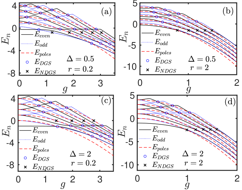
Figure 1: (Color online) The spectra and the isolated exceptional solutions for the anisotropic QRM for $\Delta=0.5$ (upper panel) and $\Delta=2$ (lower panel), $r=0.2$ (left panel) and $r=2$ (right panel). Open circles are obtained from Eq. (15), crosses are determined by zeros of the special G-functions Eq. (23).

We will shown in the next section that the open circles correspond to degenerate exceptional solutions and the crosses to non-degenerate exceptional solutions. Both are accompanied by the lifting of a pole in both $G_{+}(x)$ and $G_{-}(x)$ (circles) or in only one of them (crosses). The latter solutions can be obtained by a transcendental $G$-function, given in Eq. (23), dedicated to the non-degenerate exceptional spectrum Wakayama ; braak-fmi while the former are characterized by algebraic equations for the model parameters (the quasi-exact or “Juddian” solutions).

If $g_{1}=g_{2}=g$, the $G$-function of the isotropic QRM Braak is recovered. Note that the ground state in the isotropic QRM always has even parity because it is continuously connected to the trivial case $g=0$ which has even parity according to the definition of $\hat{\Pi}$.

III The exceptional spectrum

From Eq. (7), one notes that the coefficient $e_{n}$ diverges at $x=n$ due to its denominator if

$$E=n-\lambda_{+}.$$ (14)

Energies of this form are excluded from the regular spectrum, because they corresponds to poles, not zeros of $G_{\pm}(x)$. But let’s assume there is nevertheless a state with energy $E=n-\lambda_{+}$. In this case the numerator of the right-hand-side of Eq. (7) should vanish at $x=n$ so that $e_{n}$ remains finite, which results in two cases, i.e. either (A),

$$\left(\beta-\frac{\lambda_{+}}{\beta}\right)e_{n-1}+\left(\frac{1}{2}\Delta-\lambda_{-}\right)f_{n}+\frac{\lambda_{-}}{\beta}f_{n-1}=0,$$ (15)

with nonzero $e_{n-1},f_{n},$ and $f_{n-1}$, or (B),

$$e_{n-1}=0,f_{n}=0,f_{n-1}=0.$$ (16)

These two requirements correspond either to a doubly degenerate eigenvalue (case (A)) or a special non-degenerate state (case (B)). Both have the energy $E=n-\lambda_{+}$ and are associated with the $n$-th pole line of $G_{\pm}(x)$. Energies of this form comprise the degenerate and non-degenerate exceptional spectrum.

III.1 Degenerate exceptional states

Equation (15) provides a constraint on the model parameters. This constraint is actually a necessary and sufficient condition for the occurrence of a doubly degenerate eigenvalue without specified parity, because the pole at $x=n$ is lifted in both $G_{+}(n)$ and $G_{-}(n)$ and neither function vanishes or diverges at the exceptional energy parameter $x=n$. The model parameters $\{g,\Delta,r\}$ satisfying Eq. (15) indicate therefore a level crossing in the spectral graph located on the pole line $E(g,r)=n-\lambda_{+}(g,r)$.

By eliminating the $e_{i}$, Eq. (15) can be written explicitly as

$$F_{n}(g)=\sum_{i=0}^{n}\Gamma_{i}\left(n\right)f_{i}=0$$ (17)

where

$$\Gamma_{i}\left(n\right)=\frac{\left(\frac{\lambda_{+}}{\beta}-\beta\right)^{\left(n-i\right)}}{\left(n-i\right)!}\left[\left(\frac{n-i}{\lambda_{+}-\beta^{2}}-1\right)\lambda_{-}+\frac{1}{2}\Delta\right]$$

Given the parameters $\Delta$ and $r$, the coupling strength $g_{k}^{(n)}$ where the doubly degenerate state on the $n$-the pole line occurs follows from Eq. (17). In general, there is more than one solution for given $n$, these solutions are labeled here with the index $k$. These states are marked with open circles in Fig. 1. Let us analyze these doubly degenerate states in detail below.

For $n=0$, $x=0$, the solution is unique and given by

$$g_{1}^{(0)}=\sqrt{\frac{\Delta}{1-r^{2}}},$$ (18)

which is the same as Eq. (11) in Ref. Fanheng using the Bargmann space approach and Eq. (15) in Ref. Duan2015 . It follows that the first excited state and the ground state can only intersect if the CRW coupling is different and weaker than the RW one. The parity in the lowest energy state switches passing through this point, so a first-order quantum phase transition occurs at $g_{1}^{(0)}$, in sharp contrast with the isotropic QRM. From Eq. (18), the first level crossing in the left panel of Fig. 1 occurs at $g_{1}^{(0)}=0.7217$ and $1.4434$ for $r=0.2,$ $\Delta=0.5$ and $2$, respectively, consistent with numerical calculations. As shown in the right panel of Fig. 1, the first two levels do not cross. No real solutions exist for $r>1$.

For the second pole line, $n=1,x=1$, Eq. (17) reduces to a cubic equation for $y=g^{2}$ as

$$2y\left(1+r^{2}\right)-1+\frac{\Delta^{2}-y^{2}\left(1-r^{2}\right)^{2}}{4}+\frac{2}{\frac{\Delta}{y\left(1-r^{2}\right)}-1}=0.$$ (19)

Unlike Eq. (18), real solutions of Eq. (19) and Eq. (17) for all $n>1$ exist for $r>1$.

Surprisingly, as shown in the left panel of Fig. 1, the first two levels seem to intersect the pole line $n=1$ after they have intersected the line $n=0$ at $g_{1}^{(0)}$. Is this a true level crossing or a numerical artefact? To this end, we replot the spectral graph for $\Delta=0.5$, $r=0.2$ and $2$, for the first four levels in Figs. 2 (a) and  2 (c), respectively. In Figs. 2 (b) and (d) we plot the functions $F_{1}(g)$ and $F_{2}(g)$ whose zeros give the position of the couplings where the level crossings occur. This shows that although the crossings are barely recognizable in the plots of the left panels, only revealed on an enlarged scale (insets), the functions in the right panels exhibit the double degenerate points clearly. On sees that for $r<1$ the ground state parity changes at level crossings with the first excited state at the pole lines $n=0,1,2$ for increasing $g$, whereas the parity change occurs also for $r>1$ but at level crossings belonging to $n=1,2$, as the line $n=0$ does not support a degeneracy for $r>1$. These quantum phase transitions for $r>1$ happen only in the deep strong coupling limit (for $r=2$, $g/g_{c}\sim 6$), where the ground state and the first excited state are almost degenerate anyway.

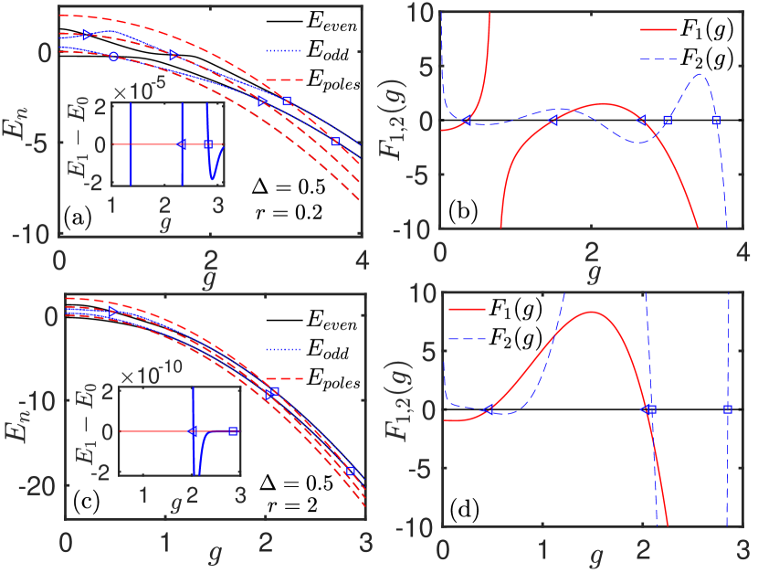
Figure 2: (Color online) The spectra for the first $4$ levels and the degenerate exceptional solutions for the anisotropic QRM with anisotropic constant $r=0.2$ (upper panel) and $r=2$ (low panel) for $\Delta=0.5$. Solutions to Eq. (17) are marked with open symbols: $n=0$ (circle), $n=1$ (triangle), and $n=2$ (square). The zeros of $F_{1,2}(g)$ corresponding to open symbols in the left panels are indicated by the same symbols in the right panels. Note that some zeros associated with level crossings of states above those present in the left panels are not marked with symbols.

To show the level crossings more clearly, we present the energy spectra $E+\lambda_{+}$ as a function of the coupling $g$ in Fig. 3. The pole lines are now horizontal(red dashed lines). The most interesting feature of the AiQRM, which sets it apart from the isotropic QRM, is the fact that for increasing $g$, the ground state rises in energy compared to the pole lines. In the isotropic case $r=1$, the ground state never crosses the first pole line $n=0$ (middle panels in Fig. 3) and the asymptotic energies in the deep strong coupling regime are the pole energies (all energies are asymptotically doubly degenerate). In the AiQRM for $r\neq 1$, the GS energy crosses all pole lines for $n>1$ if the coupling grows and this allows for a succession of first order phase transitions if these crossings belong to the degenerate exceptional spectrum. This is not necessary the case, because they could also be non-degenerate exceptional solutions, discussed in Sec. III.2. However, we find that the largest zero $g^{(n)}_{\text{max}}$ of $F_{n}(g)$ always corresponds to a crossing of the ground state and the first excited state because all non-degenerate exceptional solutions $g^{(n)}_{\text{n.d.}}$ for given $n$ satisfy $g^{(n)}_{\text{n.d.}}<g^{(n)}_{\text{max}}$.

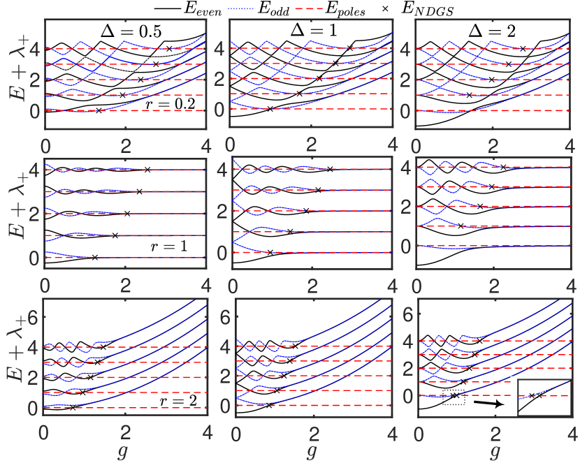
Figure 3: (Color online) The spectra $E+\lambda_{+}$ for the anisotropic QRM at $\Delta=0.5$ (left panel), $1$ (middle panel), and $2$ (right panel). $r=0.2$ (upper panel), $r=1$ (middle panel), and $r=2$ (lower panel). Crosses denote the non-degenerate solutions determined by zeros of the special G-functions Eq. (23).

Quasi-exactness of the doubly degenerate eigenvalues:- For a doubly degenerate eigenvalue $E=m-\lambda_{+}$, the model parameters satisfy Eq. (15). This means that $e_{m}$ is not determined by the recurrence relations and may take an arbitrary value before normalizing the wave function. If we fix it to

$$\;e_{m}=\frac{\left[\frac{\lambda_{-}}{\beta}e_{m-1}+\left(2\beta^{2}+2\lambda_{+}\right)f_{m}-\left(\beta+\lambda_{+}/\beta\right)f_{m-1}\right]}{\left(\frac{1}{2}\Delta+\lambda_{-}\right)},$$

we have $f_{m+1}=e_{m+1}=0$. It can be easily shown that all coefficients $f_{k}$ and $e_{k}$ for $k>m$ vanish whereas the coefficients $e_{n},f_{n}$ for $n<m$ are defined by the recurrence relations (7) and (8). This leads to the expression of one of the doubly degenerate eigenfunctions in terms of the first ECS,

$$\left|A_{+}\right\rangle_{m}=\left(\begin{array}[]{c}\sum_{n=0}^{m}\sqrt{n!}e_{n}|n\rangle_{A_{+}}\\ \sum_{n=0}^{m}\sqrt{n!}f_{n}|n\rangle_{A_{+}}\end{array}\right).$$ (20)

This eigenfunction has no fixed parity, but it can be written as a finite polynomial in the shifted oscillator states $|n\rangle_{A_{+}}$. Applying now the parity operator $\hat{\Pi}$ to this state, we obtain

$$\left|A_{-}\right\rangle_{m}=\left(\begin{array}[]{c}\sum_{n=0}^{m}\left(-1\right)^{n}\sqrt{n!}f_{n}|n\rangle_{A-}\\ \sum_{n=0}^{m}\left(-1\right)^{n}\sqrt{n!}e_{n}|n\rangle_{A-}\end{array}\right),$$ (21)

which is obviously another state with energy $m-\lambda_{+}$, linearly independent from $\left|A_{+}\right\rangle_{m}$. Both states have a finite expansion in their respective ECS bases but the expansion in the original bosonic Fock states does not terminate, in contrast to the “dark states” occurring in the Dicke models jie .

In the isotropic QRM, the proof is even simpler. If $E=m-g^{2}$, which is the $m$-th pole energy, then the condition for double degeneracy reads

$$f_{m}(x)=0,$$ (22)

using

$$\left(m-g^{2}-E\right)e_{m}=\frac{\Delta}{2}f_{m},$$

Thus $e_{m}$ would be arbitrary. If we set

$$e_{m}=-\frac{4g}{\Delta}f_{m-1},$$

then $f_{m+1}=0$, further $e_{m+1}=0$. Because both $f_{m}$ and $f_{m+1}$ are zero, $f_{m+2}$ and $e_{m+2}$ vanish as well. In this case the coefficients $f_{k}$ and $e_{k}$ for $k>m+1$ vanish, thus one of the degenerate eigenfunctions is given as a finite polynomial in the ECS basis $\{\left|n\right\rangle_{A_{+}}\}$ (see also Braak19 ). These states are the quasi-exact solutions of the QRM found originally by Judd Judd ; Koc .

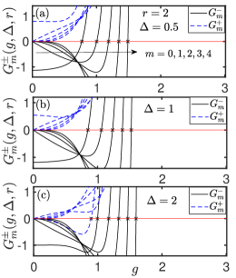
Figure 4: (Color online) The special $G$-functions $G_{m}^{\pm}(g,\Delta,r)$ for $r=2$. Their zeros give the non-degenerate exceptional solutions $g^{(m)}_{\text{n.d.}}$, i.e. crossings with the pole line $m$. These are depicted as crosses in the lower panel of Fig. 3. Note that for large $\Delta$, the line $m=0$ supports non-degenerate exceptional solutions of both parities for $g\sim 1$.

III.2 Non-degenerate exceptional states

The non-degenerate exceptional states correspond also to states with $E=m-\lambda_{+}$ but this energy is non-degenerate because the pole at $x=m$ is only lifted in one of the $G$-functions, $G_{+}(x)$ or $G_{-}(x)$, but not in both. The state is therefore a parity eigenstate. These states have been first analyzed for the QRM with the Bargmann space technique in Maciejewski21 and later in Braak19 and braak-fmi .

We shall analyze them now with the ECS technique for the AiQRM. If condition (16) holds, $e_{m}$ can take an arbitrary value, while all coefficients $e_{k},f_{k}$ for $k<m$ vanish. Setting $e_{m}=1$, $f_{m}=0$ all coefficients for $e_{n}$ and $f_{n}$ with $n\geq m+1$ are fixed by the recurrence relations (7) and (8). Imposing now that the constructed state is a parity eigenstate, we find that one of the $G$-functions

$$G_{m}^{\pm}(g,\Delta,r)=\pm\beta^{m}+\sum_{n=m+1}^{\infty}\left(f_{n}\pm e_{n}\right)\beta^{n}$$ (23)

must vanish. These $G$-functions are associated with the exceptional energy $m-\lambda_{+}$ and the $m$-th pole line. They are functions of the model parameters and their vanishing puts a constraint on these parameters, similarly to Eq. (17) for the degenerate eigenvalues. The non-degenerate exceptional eigenstates are marked by crosses in Fig. 1 and correspond to zeros of either $G_{m}^{+}(g,\Delta,r)$ or $G_{m}^{-}(g,\Delta,r)$. They are not quasi-exact states like the doubly-degenerate eigenstates, because the functions $G^{\pm}_{m}(g,\Delta,r)$ are not polynomials in $\beta$.

The $G$-functions $G_{m}^{\pm}(g,\Delta,r)$, $m=0,\ldots 4$, for several $\Delta$ at $r=2$ are plotted in Fig. 4 (c.f. the lower panel in Fig. 3). We see that each of them has at most one zero at the coupling $g^{(m)}_{\text{n.d.}}$, which happens to be always smaller than $g^{(m)}_{\text{max}}$. While it would be interesting to show this conjecture analytically, we confine ourselves here to a numerical check. It entails that the AiQRM exhibits an infinite series of phase transitions for increasing coupling, similar to the Jaynes-Cummings model, not only for $r<1$, where the RW terms dominate but also in the dual case $r>1$.

IV Ground state instability

The intersections of energy levels in the spectral graph are directly related to the symmetries of the Hamiltonian. In the case of the isotropic QRM and the AiQRM, we have seen that all level crossings in these models have the same origin, namely the manifest $\mathbb{Z}_{2}$-symmetry. The crucial feature of these degeneracies is that they are located always on the lines where the $G$-functions have poles. If the ground state energy crosses one of these lines, as is the case for any non-vanishing anisotropy ($r\neq 1$), the concomitant degeneracy of the ground state indicates a quantum phase transition of first order, where the symmetry of the ground state is not defined. The otherwise well-defined parity of the ground state changes sign upon crossing these points. Because the ground state energy crosses eventually all pole lines in the AiQRM, the system undergoes infinitely many such phase transitions for increasing coupling. The ground state phase diagram in the $g/r$-plane is shown in Fig. 5 for three different values of $\Delta$. The parity of the ground state in the different phases is either $+1$ or $-1$. The parity is unique and positive in a region around the isotropy line $r=1$, while we recover the infinitely many phase transitions of the Jaynes-Cummings model for $r=0$. The phase diagram for $r<1$ is consistent with that proposed recently by Ying using numerical exact diagonalization yingzj .

In principle, the crossing of an energy level with a pole line could be due to a non-degenerate exceptional eigenstate [as in Figs. 1  (b) and  1 (d)] and would not indicate a quantum phase transition. However, our numerical checks have shown so far that all maximal solutions of Eq. (17) belong indeed to a degeneracy of the ground state, although most of them occur in the deep strong coupling regime, where we have already almost perfect degeneracy of the two lowest energy eigenstates.

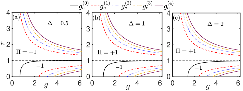
Figure 5: (Color online) The phase diagram in the $r/g$ plane for the AiQRM at $\Delta=0.5$ (left panel), $1$ (middle panel), and $2$ (right panel). $g_{c}^{(n)}$ is the maximum among the solutions $g_{k}^{(n)}$ of Eq. (17) for given $n$. The isotropy line $r=1$ (dashed) separates the two regions of the phase diagram where multiple quantum phase transitions are possible. The line $r=0$ denotes the Jaynes-Cummings model.

Finally, we would like to point out that the switch between even and odd parity of the ground state has been observed in the anisotropic spin-boson model by two of the present authors yanzhi . As shown in the top area of Fig. 1(a) in that paper, a delocalized phase with even parity switches to a delocalized phase with odd parity with increasing coupling strength in the highly anisotropic system.

V Conclusions

In this work, we derive the two parity $G$-functions for the anisotropic quantum Rabi model employing its manifest $\mathbb{Z}_{2}$-symmetry by the Bogoliubov operator (ECS) approach in the physical Hilbert space $L_{2}(\mathbb{R})$. Zeros of the $G$-functions yield the regular spectrum with well-defined parity. The exceptional solutions are located at the pole lines of these $G$-functions and comprise all doubly degenerate eigenvalues. The condition for their occurrence is derived in closed form. This allows us to identify an infinity of first-order quantum phase transitions in the AiQRM, whenever the model is not fully isotropic. The importance of the analytical treatment becomes clear as in many cases the numerical resolution of the spectra is very difficult, especially in the deep strong coupling regime (see Fig. 1).

At each crossing of the two lowest energy states the parity of the ground state switches between the discrete values $+1$ and $-1$ for increasing coupling strength. For the extreme case $r=0$ (Jaynes-Cummings model), the value of the excitation number $\hat{N}$ rises by $+1$ at each phase transition point. While $\hat{N}$ is not conserved for $r\neq 0$, the infinite number of phase transitions remains in the anisotropic case at any value $r\neq 1$. The only model with no phase transition in the ground state for any coupling is the isotropic QRM. The rich phase diagram of the AiQRM is solely due to its manifest $\mathbb{Z}_{2}$-symmetry. In contrast, the level crossings of higher excited states occurring at special values of the symmetry-breaking parameter $\epsilon$ in the asymmetric QRM (where the $\mathbb{Z}_{2}$-symmetry is broken by the term $\epsilon\sigma_{x}$ in the Hamiltonian) is due to a non-manifest, hidden symmetry bat ; ash2020 ; man ; rey .

^† daniel.braak@physik.uni-augsburg.de

^∗ qhchen@zju.edu.cn

References

- (1) I. I. Rabi, Phys. Rev. 49, 324 (1936); 51, 652 (1937).
- (2) M. O. Scully, and M. S. Zubairy, Quantum Optics (Cambridge University Press, Cambridge, 1997); M. Orszag, Quantum Optics Including Noise Reduction,Trapped Ions, Quantum Trajectories, and Decoherence (Springer, Berlin, 2007), 2nd ed.
- (3) E. T. Jaynes and F. W. Cummings, Proc. IEEE 51, 89 (1963)
- (4) A. Wallraff et al., Nature (London) 431, 162 (2004).
- (5) F. Deppe et al., Nature Physics 4, 686 (2008).
- (6) T. Niemczyk et al., Nature Physics 6, 772 (2010).
- (7) P. Forn-Díaz et al., Phys. Rev. Lett. 105, 237001 (2010).
- (8) F. Yoshihara, T. Fuse, S. Ashhab, K. Kakuyanagi, S. Saito, and K. Semba, Nat. Phys. 13, 44 (2016).
- (9) J. Casanova et al., Phys. Rev. Lett. 105, 263603 (2010);
- (10) J. Hausinger and M. Grifoni, Phys. Rev. A80, 062320(2010).
- (11) S. Ashhab and F. Nori, Phys. Rev. A 81, 042311 (2010); S. Ashhab, Phys. Rev. A 87, 013826 (2013).
- (12) S. He et al., Phys. Rev. A 86, 033837 (2012); ibid 90, 053848 (2014).
- (13) I. D. Feranchuk, L. I. Komarov, and A. P. Ulyanenkov, J. Phys. A: Math. Gen. 29 4035 (1996).
- (14) E. K. Irish, Phys. Rev. Lett. 99, 173601 (2007).
- (15) C. J. Gan and H. Zheng, Eur. Phys. J. D 59, 473 (2010).
- (16) D. Braak, Phys. Rev. Lett. 107, 100401 (2011).
- (17) H.-H. Zhong, Q.-T. Xie, M. T. Batchelor, and C.-H. Lee , J. Phys. A 46, 415302 (2013); J. Phys. A 47, 045301 (2014).
- (18) L. W. Duan, Y.-F. Xie, D. Braak, Q.-H. Chen, J. Phys. A: Math. Theor. 49, 464002 (2016).
- (19) D. Braak, Symmetry 11, 1259 (2019).
- (20) M. Wakayama and T. Yamasaki, J. Phys. A: Math. Theor. 47, 335203 (2014).
- (21) Q. H Chen, C. Wang, S. He, T. Liu, and K. L. Wang, Phys. Rev. A 86, 023822 (2012).
- (22) K. Furuya, M. C. Nemes, and G. Q. Pellegrino, Phys. Rev. Lett. 80, 5524(1998)
- (23) Y. X. Yu, J. Ye, and W. M. Liu, Scientific Reports 3, 3476(2013).
- (24) Q. T. Xie, S. Cui, J. P. Cao, L. Amico, and H. Fan, Phys. Rev. X 4, 021046 (2014).
- (25) M. Tomka, O. E. Araby, M. Pletyukhov, and V. Gritsev, Phys. Rev. A90, 063839 (2014).
- (26) S. I. Erlingsson, J. C. Egues, and D. Loss, Phys. Rev. B 82, 155456 (2010).
- (27) M. Schiró, M. Bordyuh, B. Öztop, and H. E. Türeci, Phys. Rev. Lett. 109, 053601 (2012).
- (28) A. L. Grimsmo and S. Parkins, Phys. Rev. A 87, 033814 (2013).
- (29) F. Mivehvara, F. Piazzab, T. Donnerc, and H. Ritsch, arXiv: 2102.04473 (2021).
- (30) D. Braak, in Proceedings of the Forum of Mathematics for Industry 2014 , edited by R. S. Anderssen et al. (Springer, Tokyo, 2016), p. 75.
- (31) L. W. Duan and Q. H. Chen, arXiv:1502.00487 (2015).
- (32) Z.-J. Ying, arXiv:2010.15113 (2020).
- (33) Q. H. Chen, Y. Y. Zhang, T. Liu, and K. L. Wang, Phys. Rev. A 78, 051801(R) (2008).
- (34) J. Peng et al., J. Phys. A: Math. Theor. 47, 265303 (2014).
- (35) B. R. Judd, J. Phys. C 12, 1685 (1979).
- (36) R. Koc, M. Koca, and H. H. Tütüncüler, J. Phys. A: Math. Gen. 35, 9425(2002).
- (37) A. J. Maciejewski, M. Przybylska, and T. Stachowiak, Phys. Lett. A 378, 16(2014)
- (38) Y.-Z. Wang, S. He, L. W. Duan, and Q.-H. Chen, Phys. Rev. B 101, 155147 (2020).
- (39) Z.M. Li and M.T. Batchelor, J. Phys. A: Math. Theor. 48, 454005 (2015).
- (40) S. Ashhab, Phys. Rev. A 101, 023808 (2020).
- (41) V. Mangazeev, M.T. Batchelor and V.V. Bazhanov, J. Phys. A: Math. Gen. 54, 12LT01 (2021).
- (42) C. Reyes-Bustos, D. Braak and M. Wakayama, arXiv:2101.04305 (2021).