A deep learning algorithm for optimal investment strategies

Abstract

This paper treats the Merton problem how to invest in safe assets and risky assets to maximize an investor’s utility, given by investment opportunities modeled by a $d$-dimensional state process. The problem is represented by a partial differential equation with optimizing term: the Hamilton–Jacobi–Bellman equation. The main purpose of this paper is to solve partial differential equations derived from the Hamilton–Jacobi–Bellman equations with a deep learning algorithm: the Deep Galerkin method, first suggested by Sirignano and Spiliopoulos (2018). We then apply the algorithm to get the solution of the PDE based on some model settings and compare with the one from the finite difference method.

1 Introduction

Consider the following expected utility maximization problem:

$$\max_{(\pi_{u})_{u\geq t}}\frac{1}{p}\,\mathbb{E}\left[(X^{\pi}_{T})^{p}\,|\,X_{t}=x,\,Y_{t}=y\right],$$ (1.1)

where $\pi$ is a portfolio, $X^{\pi}$ a wealth process and $Y$ a state variable with the utility function $(1/p)x^{p}=:U(x)$. This kind of problem is first suggested by Merton (1969), which is the most fundamental and pioneering in economics. The Merton problem has played as a key for an investor’s wealth allocation in several assets under some market circumstances. Since then there have been lots of studies about Merton problem under various conditions. Benth et al. (2003) studied Merton problem under the Black-Scholes setting by using the OU type stochastic volatility model. Kühn and Stroh (2010) studied optimizing portfolio of Merton problem under a limit-ordered market in view of a shadow price. The research on the optimal investment based on inside information and drift parameter uncertainty was conducted by Danilova et al. (2010). Nutz (2010) studied the utility maximization in a semimartingale market setting with the opportunity process. Hansen (2013) suggested an optimal investment strategies with investors’ partial and private information. Pedersen and Peskir (2017) applied the Lagrange multiplier to solve nonlinear mean-variance optimal portfolio selection problem. Also there was research on the optimal portfolio strategies using over-reaction and under-reaction by Callegaro et al. (2017). Liang and Ma (2020) researched a robust Merton problem using the constant relative/absolute risk aversion utility functions under the time-dependent sets of confidence.

In this paper we follow the overall market setting in Guasoni and Robertson (2015) and induce the so-called Hamilton–Jacobi–Bellman equation under time variable $t$, variable $x$ representing wealth process and variable $y=(y_{1},\ldots,y_{d})$ from the $d$-dimensional state variable. We can optimize the portfolio by means of finding a solution to the HJB equation. By using some properties including homotheticity and concaveness, we eliminate the optimizing term to change the HJB equation into a nonlinear partial differential equation.

Under this circumstance we face with the problem of solving nonlinear PDEs. Because in general most PDEs do not have analytic solutions, there exists several well-known numerical tools. These classical approaches can be found in Achdou and Pironneau (2005) and Burden et al. (2010).

At the same time there has been some studies about solving PDEs with a deep neural network. Lee and Kang (1990), Lagaris et al. (2000) suggested the neural network algorithm on a fixed mesh. Malek and Beidokhti (2006) also suggested the numerical hybrid DNN optimizing method. However in case of the higher dimension of PDEs, these grid-based methods would be computationally inefficient: a curse of dimensionality.

Recently there have been several researches to get rid of the curse of dimensionality using machine learning techniques. Han et al. (2018) and Weinan et al. (2019) suggested a deep backward stochastic differential equation method with the Feynman–Kač formula.

The deep learning algorithm mainly used in this paper is the Deep Galerkin method suggested by Sirignano and Spiliopoulos (2018). It is computationally efficient since there does not need to make any mesh or grid. We define a loss functional to minimize $L^{2}$-norm about the desired differential operator and other conditions from the PDE. To make the loss small enough as we want, we sample random points from the domain and optimize by means of stochastic gradient descent. After deriving surfaces, we also apply the finite difference method(FDM) in order to compare surfaces from both algorithms: DGM and FDM. For further research on the Deep Galerkin method, see Al-Aradi et al. (2018) and Al-Aradi et al. (2019).

This paper is organized as follows. In section 2, we start by describing the general setting of this paper, and induce the partial differential equation with optimizing term: the HJB equation. The Deep Galerkin method algorithm and neural network approximation theorem from Sirignano and Spiliopoulos (2018) are presented in section 3, with some part of code for each step of DGM algorithm. Numerical test of the algorithm is presented in section 4. Specifically, we model $2$ dimensional state process by the OU process and the CIR process, return process by the Heston model. Then we use the calibrated parameters from Crisóstomo (2014) and Mehrdoust and Fallah (2020). We display the solution surface at each fixed time in some pre-determined domain of the state variable. We finally analyze surfaces from the Deep Galerkin method and those from the finite difference method. Conclusions can be found in section 5, and proofs of neural network approximation theorem are in appendix A.

2 Optimal Investment Problem

In the case that an economic agent is in time interval $[0,T]$, the problem is that he or she has to decide how to invest in several risky assets or safe assets as time goes by, starting with the initial wealth. This problem was first suggested by Merton in the 1960s: Merton problem, known as a utility maximization problem. The aim of the agent is to establish a portfolio strategy in such a way of maximizing utility under some conditions. In this section we describe the general setting of this paper, and induce the HJB equation. We finally reach to a nonlinear PDE by using some properties. The above problem is equivalent to a matter of finding a solution of the equation.

2.1 Market with the Merton Problem

We first start by describing market with the following framework. Assume that the market has $n+1$ assets $S^{(0)},S^{(1)},\ldots,S^{(n)}$, where $S^{(0)}$ is safe and $S^{(1)},\ldots,S^{(n)}$ are risky. One can make a decision to the investment by a $d$-dimensional state variable $Y=(Y^{(1)},\ldots,Y^{(d)})$ satisfying:

$$dY_{t}=b(Y_{t})\,dt+a(Y_{t})\,dW_{t},$$ (2.1)

where $W=(W^{(1)},\ldots,W^{(d)})$ denotes a standard Brownian motion.

Let $r$ be the interest rate, $\mu$ be the excess returns, and $\sigma$ be the volatility matrix. We also assume that the prices of the assets satisfy:

$$dS^{(0)}_{t}=rS^{(0)}_{t}dt,$$ (2.2)

$$\dfrac{dS^{(i)}_{t}}{S^{(i)}_{t}}=rdt+dR^{(i)}_{t}\qquad 1\leq i\leq n,$$ (2.3)

where $R=(R^{(1)},\ldots,R^{(n)})$ denotes the cumulative excess return satisfying:

$$dR^{(i)}_{t}=\mu_{i}(Y_{t})dt+\sum_{j=1}^{n}\sigma_{ij}(Y_{t})\,dZ^{(j)}_{t}\qquad 1\leq i\leq n.$$ (2.4)

$\rho=(\rho_{ij})=d\left\langle Z,\,W\right\rangle_{t}/dt$ denotes the cross correlations between the $n$-dimensional Brownian motion $Z$ and $W$. $\Sigma=\sigma\sigma^{T}=d\left\langle R,\,R\right\rangle_{t}/dt$ is the matrix of quadratic covariance of returns, and $\Upsilon=\sigma\rho a^{T}=d\left\langle R,\,Y\right\rangle_{t}/dt$ denotes the correlation between the return and the state process.

In the market, an investor buys the risky assets by a portfolio $\pi=(\pi^{(1)}_{t},\ldots,\pi^{(n)}_{t})_{t\geq 0}$. The wealth process $X^{\pi}=(X^{\pi}_{t})_{t\geq 0}$ corresponding to the portfolio satisfies

$$\dfrac{dX^{\pi}_{t}}{X^{\pi}_{t}}=r\,dt+\pi^{T}_{t}\,dR_{t},\quad X^{\pi}_{0}\geq 0.$$ (2.5)

Observe first that the portfolio process $(\pi_{t})_{t\geq 0}$ is $\mathcal{F}_{t}$-measurable, where the filtration $\mathcal{F}=(\mathcal{F}_{t})_{t\geq 0}$ is generated by the return $R$ and state variable $Y$. It might be clear in light of the investor’s eyes: he or she has all informations about state and asset return from time $t=0$ to the current time. Note also the portfolio process is integrable with respect to the return process $R$. By the Merton problem, we assume the investors’ utility function is defined by the following:

$$U(x)=\dfrac{1}{p}x^{p},\quad 0<p<1.$$ (2.6)

For fixed wealth $x$ and state $y=(y_{1},\ldots,y_{d})$ satisfying (2.1) and (2.5), our aim is to maximize the conditional expectation of terminal wealth utility given wealth and state at time $t$, that is

$$\max_{(\pi_{u})_{u\geq t}}\frac{1}{p}\,\mathbb{E}\left[(X^{\pi}_{T})^{p}\,|\,X_{t}=x,\,Y_{t}=y\right].$$ (2.7)

2.2 The Hamilton–Jacobi–Bellman Equation

Now we substitute the problem of utility maximization to that of solving the PDE, namely the Hamilton–Jacobi–Bellman equation. There needs to be some definitions before approaching to the HJB equation.

Definition 2.1.

A portfolio process $\pi=(\pi_{t})_{t\geq 0}$ is called an admissible portfolio if

• For every $t\in[0,T]$ and $(x,y)\in D\subset\mathbb{R}\times\mathbb{R}^{d}$, $\pi(t,x,y)\in U$, where $U\subset\mathbb{R}$ is a fixed subset.

• For any given initial points $(t,x)$ and $y=(y_{1},\ldots,y_{d})$, the following SDE has a unique solution:

  $$dX^{\pi}_{s} =rX^{\pi}_{s}\,ds+\pi^{T}_{s}\,dR_{s},$$ (2.8)

  $$X^{\pi}_{t} =x.$$

• For any given initial point $(t,y)=(t,y_{1},\ldots,y_{d})$, the following SDE has a unique solution:

  $$dY_{s} =b(Y_{s})\,ds+a(Y_{s})\,dW_{s},$$ (2.9)

  $$Y_{t} =y.$$

By now we assume the portfolio $\pi$ is admissible.

Definition 2.2.

Let $U$ be an investor’s utility function.

• For each $\pi$, we define the expected value function $\mathcal{V}^{\pi}$ as

  $$\mathcal{V}^{\pi}(t,x,y)=\mathbb{E}[U(X^{\pi}_{T})|X_{t}=x,\,Y_{t}=y],$$ (2.10)

  given (2.8) and (2.9).

• We define the optimal value function $V$ as

  $$V(t,x,y)=\sup_{\pi}\mathcal{V}^{\pi}(t,x,y).$$ (2.11)

The following theorem justifies a conversion from the way of finding optimal portfolio to that of solving PDEs having optimizing term. Heuristic process for deriving the HJB equation is in chapter 19, Björk (2009), in the way of limiting procedures in dynamic programming.

Theorem 2.1.

Assume the following.

• The market has a safe asset $S^{(0)}$ whose dynamics is expressed in (2.2).

• The market has $n$ risky assets satisfying (2.3), with the return process $R$ following the diffusion (2.4).

• There exists an optimal portfolio $\hat{\pi}=(\hat{\pi}^{(1)}_{t},\ldots,\hat{\pi}^{(n)}_{t})_{t\geq 0}$.

• The optimal value function $V$ is regular, that is, $V\in C^{1,2,2}$ with respect to $(t,x,y)$, $y=(y_{1},\ldots,y_{d})$.

Then the following hold:

1. $V$ satisfies the Hamilton–Jacobi–Bellman equation

   $$V_{t}+b^{T}(\nabla_{y}V)+\dfrac{1}{2}\,\text{tr}[a^{T}(\nabla^{2}_{y}V)\,a]+rxV_{x}$$ (2.12)

   $$+\sup_{\pi}\left[\pi^{T}(\mu V_{x}+\Upsilon(\nabla_{y}V_{x}))x+\dfrac{1}{2}x^{2}V_{xx}\pi^{T}\Sigma\pi\right] =0, (t,x,y)\in[0,T]\times D,$$

   $$V(0,x,y) =U(x), (x,y)\in D.$$

2. An optimizing term in the above equation can be achieved by $\pi=\hat{\pi}$:

   $$\sup_{\pi}\left[\pi^{T}(\mu V_{x}+\Upsilon(\nabla_{y}V_{x}))x+\dfrac{1}{2}x^{2}V_{xx}\pi^{T}\Sigma\pi\right]=\hat{\pi}^{T}(\mu V_{x}+\Upsilon(\nabla_{y}V_{x}))x+\dfrac{1}{2}x^{2}V_{xx}\hat{\pi}^{T}\Sigma\hat{\pi}.$$ (2.13)

If we define the optimal value function as

$$V(t,x,y_{1},\ldots,y_{d})=\sup_{(\pi_{u})_{u\geq t}}\,\mathbb{E}\left[\frac{1}{p}(X^{\pi}_{T})^{p}\,|\,X^{\pi}_{t}=x,Y_{t}^{(1)}=y_{1},\ldots,Y_{t}^{(d)}=y_{d}\right],$$ (2.14)

by Theorem 2.1 with the Itô formula, one can derive the Hamilton–Jacobi–Bellman equation from (2.14):

$$\begin{split}V_{t}+b^{T}(\nabla_{y}V)+\dfrac{1}{2}&\,\text{tr}[a^{T}(\nabla^{2}_{y}V)\,a]+rxV_{x}\\ +&\sup_{\pi}\left[\pi^{T}(\mu V_{x}+\Upsilon(\nabla_{y}V_{x}))x+\dfrac{1}{2}x^{2}V_{xx}\pi^{T}\Sigma\pi\right]=0,\end{split}$$ (2.15)

where the terminal condition of (2.15) is $V(T,\,x,\,y)=(1/p)\,x^{p}$. $\nabla_{y}V=(V_{y_{1}},\ldots,V_{y_{d}})$ and $\nabla^{2}_{y}V=\left(V_{y_{i}y_{j}}\right)_{1\leq i,j\leq d}$ stand for the gradient and the Hessian of $V$ with respect to $y=(y_{1},\ldots,y_{d})$, respectively. Because of the concaveness of $V$ in $x$ and $\sup_{\pi}(\pi^{T}b+\frac{1}{2}\pi^{T}A\pi)=-\frac{1}{2}b^{T}A^{-1}b$ for negative definite matrix $A$, (2.15) becomes

$$\begin{split}V_{t}+b^{T}(\nabla_{y}V)+\dfrac{1}{2}&\,\text{tr}[a^{T}(\nabla^{2}_{y}V)\,a]+rxV_{x}\\ -&(\mu V_{x}+\Upsilon(\nabla_{y}V_{x}))^{T}\dfrac{\Sigma^{-1}}{2V_{xx}}(\mu V_{x}+\Upsilon(\nabla_{y}V_{x}))=0,\end{split}$$ (2.16)

with the corresponding optimal portfolio is

$$\pi=\pi(t,x,y_{1},\ldots,y_{d})=-\dfrac{1}{xV_{xx}}\Sigma^{-1}(\mu V_{x}+\Upsilon(\nabla_{y}V_{x})).$$ (2.17)

Since the utility function is homothetic, we define the reduced value function $u$ as

$$V(t,x,y_{1},\ldots,y_{d})=\dfrac{1}{p}\,x^{p}\,u(t,y_{1},\ldots,y_{d}).$$ (2.18)

If we put (2.18) into (2.16) and divide each component by $x^{p}$, (2.16) becomes

$$\begin{split}u_{t}+(b^{T}-&q\mu^{T}\Sigma^{-1}\Upsilon)\nabla_{y}u+\dfrac{1}{2}\,\text{tr}[a^{T}(\nabla^{2}_{y}u)\,a]\\ +&(pr-\dfrac{q}{2}\mu^{T}\Sigma^{-1}\mu)u-\dfrac{q}{2u}(\nabla_{y}u)^{T}\Upsilon^{T}\Sigma^{-1}\Upsilon(\nabla_{y}u)=0,\end{split}$$ (2.19)

where the terminal condition of (2.19) is $u(T,y_{1},\ldots,y_{d})=1$. In (2.19), we set $q=p/(p-1)$ for simplicity. Also the following is the reduced optimal portfolio:

$$\pi(t,y_{1},\ldots,y_{d})=\dfrac{1}{1-p}\left(\Sigma^{-1}\mu+\Sigma^{-1}\Upsilon(\nabla_{y}u)\dfrac{1}{u}\right).$$ (2.20)

3 Deep Galerkin Method

Now we investigate how to solve the PDEs such as (2.19). Since only few PDEs have analytic solutions, there are well-known numerical tools including the Monte Carlo method exemplified by the Feynman–Kač theorem and the finite difference method. However one of the most difficult facts is a curse of dimensionality. In particular in grid-based numerical methods, the number of mesh points grows explosively as the dimension goes higher, so Sirignano and Spiliopoulos (2018) suggest a DNN-based algorithm for approximating solution of PDEs: the Deep Galerkin method(DGM), such that there is no need to make any mesh.

With the parametrized deep neural network, say $f$, a loss functional $f\mapsto J(f)$ is defined to minimize $L^{2}$-norm about the desired differential operator and terminal condition. To make the loss small enough as we want, the network samples random points from the pre-determined domain and is optimized by means of the stochastic gradient descent. In this section we first introduce the DGM algorithm. We then state the approximation theorem in order to justify this new algorithm.

3.1 Algorithm

Let $u=u(t,y)$ be an unknown function which satisfies the PDE:

$$\partial_{t}u(t,y)+\mathcal{L}u(t,y) =0, (t,y)\in[0,T]\times D,$$ (3.1)

$$u(T,y) =u_{T}(y), y\in D,$$

where $D\subset\mathbb{R}^{d}$. Our aim is to express the solution of (3.1) as a neural network function $f=f(t,y;\theta)$ in place of $u$. $\theta=(\theta^{(1)},\cdots,\theta^{(K)})$ denotes a vector of network parameters.

Define a loss functional $J:=J_{1}+J_{2}$ with

$$J_{1}(f) :=\lVert\partial_{t}f(t,y;\theta)+\mathcal{L}f(t,y;\theta)\rVert^{2}_{[0,T]\times D,\nu_{1}}$$ (3.2)

$$J_{2}(f) :=\lVert f(T,y;\theta)-u_{T}(y)\rVert^{2}_{D,\nu_{2}}$$

Note that all above terms are expressed in terms of $L^{2}$-norm, that is, $\lVert h(y)\rVert^{2}_{\mathcal{Y,\nu}}=\int_{\mathcal{Y}}\,\lvert h(y)\rvert^{2}\nu(y)dy$. Each functionals $J_{1}$ and $J_{2}$ determine that how well the approximation has conducted in view of the PDE differential operator and terminal condition. The aim is to find a parameter $\hat{\theta}$ in such a way of minimizing $J(f)$, equivalently,

$$\hat{\theta}=\operatorname*{arg\,min}_{\theta}J(f(t,y;\theta)).$$ (3.3)

As the error $J(f)$ goes smaller, the approximated function $f$ would get closer to the solution $u$. Hence $f(t,y;\hat{\theta})$ might be the best approximation of $u(t,y)$.

The algorithm of DGM is as follows:

1. Set initial values of $\theta_{0}=(\theta^{(1)}_{0},\cdots,\theta^{(K)}_{0})$ and determine the learning rate $\beta_{n}$.

2. Sample random points $(t_{n},y_{n})$ in $[0,T]\times D$ according to probability density $\nu_{1}$. Likewise, pick random points $w_{n}$ from $D$ with density $\nu_{2}$.

3. Calculate the $L^{2}$-error for the randomly sampled points $s_{n}=\{(t_{n},y_{n}),w_{n}\}$:

   $$L(\theta_{n},s_{n})=((\partial_{t}+\mathcal{L})f(t_{n},y_{n};\theta_{n}))^{2}+(f(T,w_{n};\theta_{n})-u_{T}(w_{n}))^{2}.$$ (3.4)

4. Use the stochastic gradient descent at $s_{n}$:

   $$\theta_{n+1}=\theta_{n}-\beta_{n}\nabla_{\theta}L(\theta_{n},s_{n}).$$ (3.5)

5. Repeat until $\lVert\theta_{n+1}-\theta_{n}\rVert$ is small enough.

The following is some part of code for each step of DGM algorithm:

⬇ # 1-1. Initializing the neural network parameter oper_init = tf.global_variables_initializer() # 1-2. Initializing the learning rate lrn_rate = tf.train.exponential_decay(init_lrn_rate, glob_step, dec_step, dec_rate, staircase=True) optimizer = tf.train.AdamOptimizer(lrn_rate).minimize(loss_tnsr) # 2-1. Generating random samples : interior of the domain t_int = np.random.uniform(low=0, high=T, size=[nSim_int,1]) y1_int = np.random.uniform(low=y1_low, high=y1_high, size=[nSim_int,1]) y2_int = np.random.uniform(low=y2_low, high=y2_high, size=[nSim_int,1]) # 2-2. Generating random samples : terminal condition t_ter = T * np.ones(nSim_ter,1) y1_ter = np.random.uniform(low=y1_low, high=y1_high, size=[nSim_ter,1]) y2_ter = np.random.uniform(low=y2_low, high=y2_high, size=[nSim_ter,1]) # 3. Calculating L^2-error of differential operator / terminal condition # differential operator J1 = tf.reduce_mean(tf.square(diff_u)) # terminal condition J2 = tf.reduce_mean(tf.square(fitted_ter - target_ter)) J = J1 + J2 # 4. Stochastic gradient descent step for k in range(steps_per_sample): loss, J1, J2, k = sess.run([loss_tnsr, J1_tnsr, J2_tnsr, optimizer], feed_dict={t_int_tnsr:t_int, y1_int_tnsr:y1_int, y2_int_tnsr:y2_int, t_ter_tnsr:t_ter, y1_ter_tnsr:y1_ter, y2_ter_tnsr:y2_ter})

3.2 Neural Network Approximation

The following neural network approximation theorem is stated in Sirignano and Spiliopoulos (2018). In other words, there exists a collection of approximated neural network functions that converges to a solution of quasilinear parabolic PDEs.

Theorem 3.1.

Define $\mathfrak{C}^{n}$ as a collection of DNN functions with $n$ hidden neurons in a single hidden layer. Assume $u=u(t,y)$ be an unknown solution for (3.1). Under certain conditions in Sirignano and Spiliopoulos (2018), there exists a neural network function $f^{n}$ with $n$ hidden neurons such that the following hold:

1. $J(f^{n})\to 0$ as $n\to\infty$,

2. $f^{n}\xrightarrow{strongly}u$ in $L^{\rho}([0,T]\times D)$ as $n\to\infty$, where $\rho<2$.

Some part of proofs for our formulation in this paper is in appendix A. Further details including conditions and proofs are in section 7 and appendix A in Sirignano and Spiliopoulos (2018).

4 Numerical Test

The key purpose of this section is to solve (2.19) with the Deep Galerkin method and compare the numerical solution with the one derived by the well-known finite difference method.

4.1 Model Settings

We first set some specific settings of the market model. For our experiment we assume that there are two ways of decision for trading, i.e., 2 dimensional state variable $Y=(Y^{(1)},Y^{(2)})$. Let $Y^{(1)}$ be the Ornstein-Uhlenbeck(OU) process and $Y^{(2)}$ be the Cox-Ingersoll-Ross(CIR) process. This state variable is expressed by the following matrix form:

$$\left(\begin{array}[]{c}dY_{t}^{(1)}\\ dY_{t}^{(2)}\end{array}\right)=\left(\begin{array}[]{c}\theta^{(1)}(k^{(1)}-Y^{(1)}_{t})\\ \theta^{(2)}(k^{(2)}-Y^{(2)}_{t})\end{array}\right)dt+\left(\begin{array}[]{cc}1&0\\ 0&\sqrt{Y^{(2)}_{t}}\\ \end{array}\right)\left(\begin{array}[]{cc}a^{(1,1)}&a^{(1,2)}\\ a^{(2,1)}&a^{(2,2)}\\ \end{array}\right)\left(\begin{array}[]{c}dW^{(1)}_{t}\\ dW^{(2)}_{t}\end{array}\right).$$ (4.1)

We also assume that there is a risky asset $S^{(1)}$ in the market, that is:

$$dS^{(1)}_{t}=rS^{(1)}_{t}dt+S^{(1)}_{t}dR_{t},$$ (4.2)

where the cumulative excess return $R$ follows the diffusion:

$$dR_{t}=Y^{(1)}_{t}\,dt+\sigma\sqrt{Y^{(2)}_{t}}\,dZ_{t},\quad(\sigma\in\mathbb{R})$$ (4.3)

which is known as the Heston model. In this case the correlation matrix between $Z$ and $W$ is of the form $\rho=(\rho_{1},\rho_{2})$ satisfying:

$$\left\langle Z,\,W^{(i)}\right\rangle=\rho_{i}\,dt,\qquad 1\leq i\leq 2.$$ (4.4)

4.2 Calibration

Now for the next step we need to set the value of parameters. Let $\mathcal{P}$ be a vector of parameters to be determined given by

$$\mathcal{P}=\left\{\theta^{(1)},\theta^{(2)},k^{(1)},k^{(2)},a^{(1,1)},a^{(1,2)},a^{(2,1)},a^{(2,2)},\sigma,\,\rho_{1},\,\rho_{2}\right\}.$$ (4.5)

We shortly introduce the calibrating process using the nonlinear least squares optimization from the market data. For more detail, see Crisóstomo (2014) and Mehrdoust and Fallah (2020).

Define the Percentage Mean Squared Error (PMSE) between the price $C_{market}$ from the market and the model price $C_{model}$ of the European call option derived from the double Heston model in Mehrdoust and Fallah (2020) and Lemaire et al. (2020):

$$\text{PMSE}:=\sum_{j=1}^{n}w_{j}\left(\dfrac{C_{market}(S^{(0)},K_{j},T_{j},r)-C_{model}(S^{(0)},K_{j},T_{j},r,\mathcal{P})}{C_{market}(S^{(0)},K_{j},T_{j},r)}\right)^{2},$$ (4.6)

where the weights $w_{j}$ satisfies:

$$w_{j}=\dfrac{1}{\sqrt{\left|C_{ask}^{(j)}-C_{bid}^{(j)}\right|}}.$$ (4.7)

The optimal parameter vector $\mathcal{P}^{\star}$ is determined by the following nonlinear least squares problem

$$\mathcal{P}^{\star}=\operatorname*{arg\,inf}\text{PMSE}.$$ (4.8)

Table 1 shows the optimal parameters on the observed market data from the S&P500 index at the close of the market in September 2010.

Table 1: Calibrated parameters

$\theta^{(1)}=0.1646$	$k^{(1)}=0.1301$	$a^{(1,1)}=-0.6594$	$a^{(1,2)}=0.7518$	$\rho_{1}=-0.2949$	$\sigma=0.0724$
$\theta^{(2)}=0.2333$	$k^{(2)}=0.0958$	$a^{(2,1)}=-0.6692$	$a^{(2,2)}=0.7431$	$\rho_{2}=-0.2919$

4.3 Implementation

Now let us solve (2.19) by the DGM algorithm under conditions from the above setting. For the numerical test, we set the interest rate $r=1\%$, the maturity time $T=1$ and the power utility preference parameters $p=0.0005$ and $p=0.5$. We sampled 1000 time-space points $(t,y_{1},y_{2})$ in the interior of the domain $[0,T]\times[-10,10]\times[0,10]$ and 100 space points at terminal time $T$. We set $100$ steps to resample new time-space domain points. Before resampling, each stochastic gradient descent step is repeated $10$ times. We set $50$ hidden neurons in a hidden layer. From starting $0.001$, learning rate decreased with decay rate 0.96 as the step goes by.

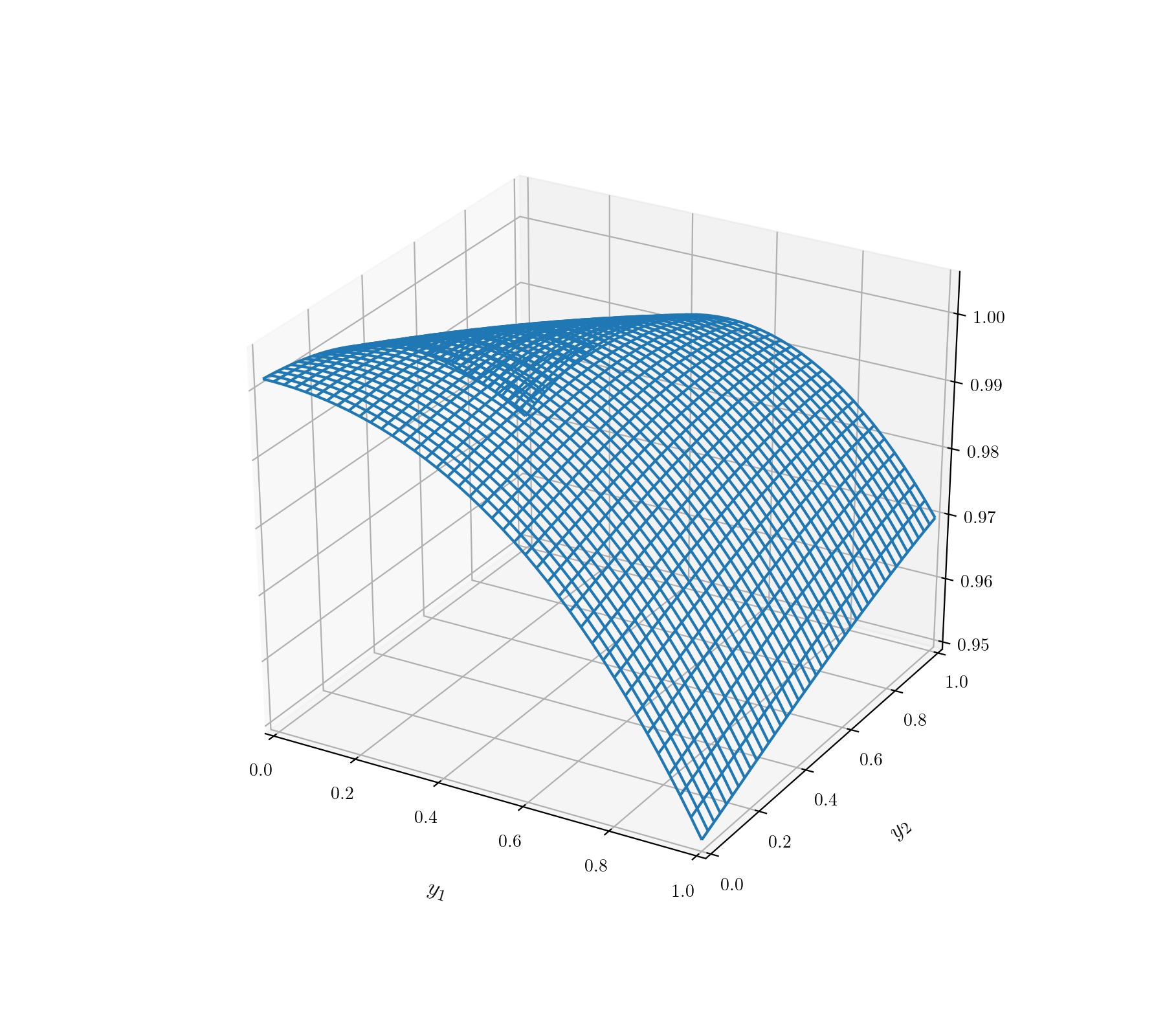
(a) $t=0$

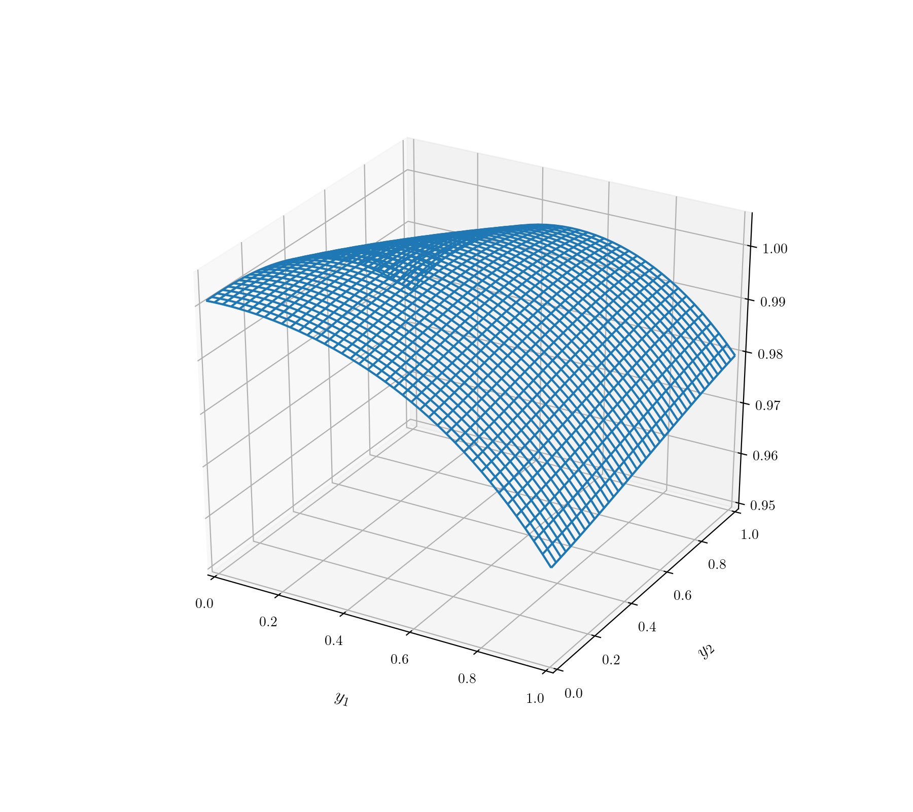
(b) $t=0.25T$

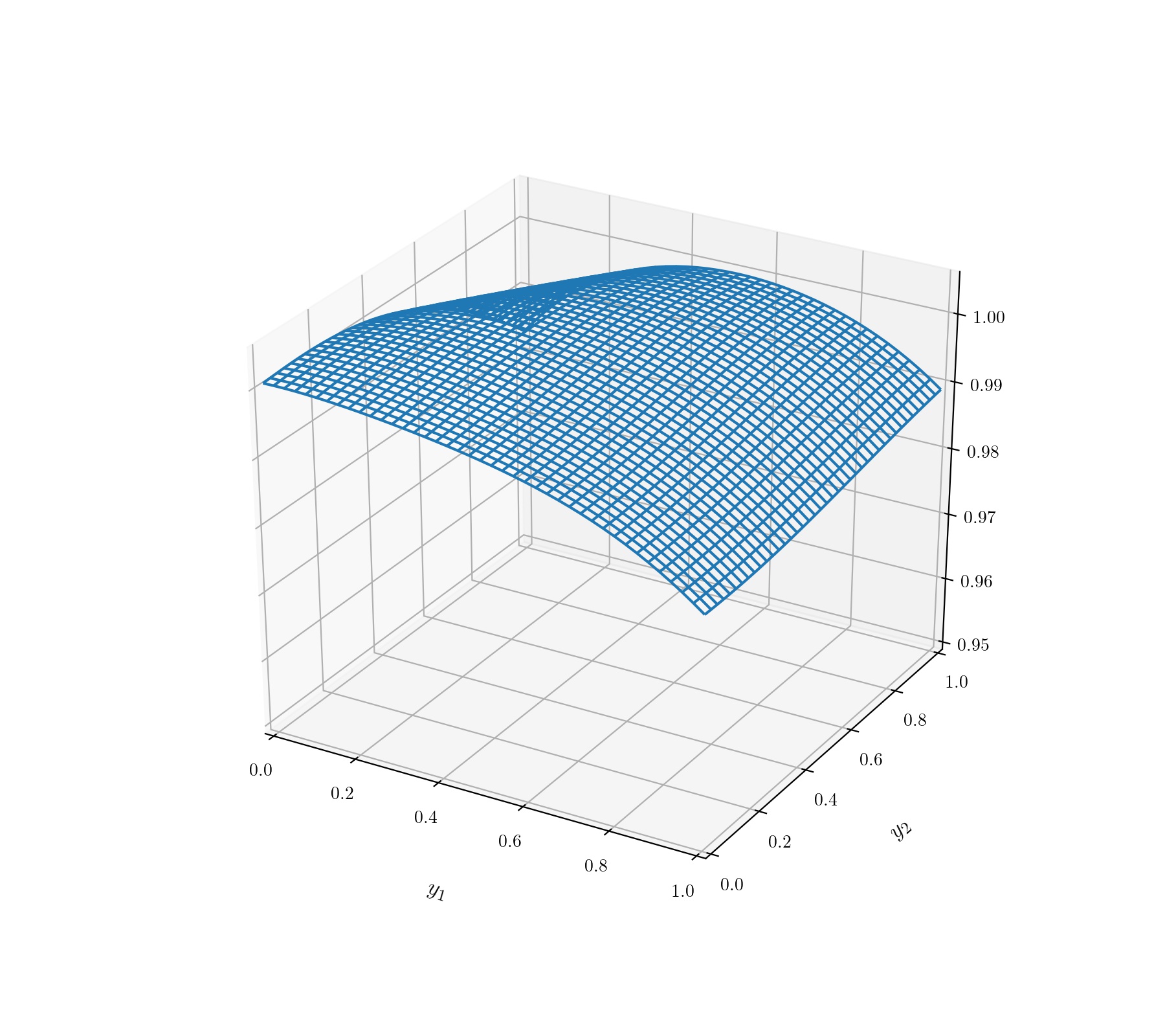
(c) $t=0.5T$

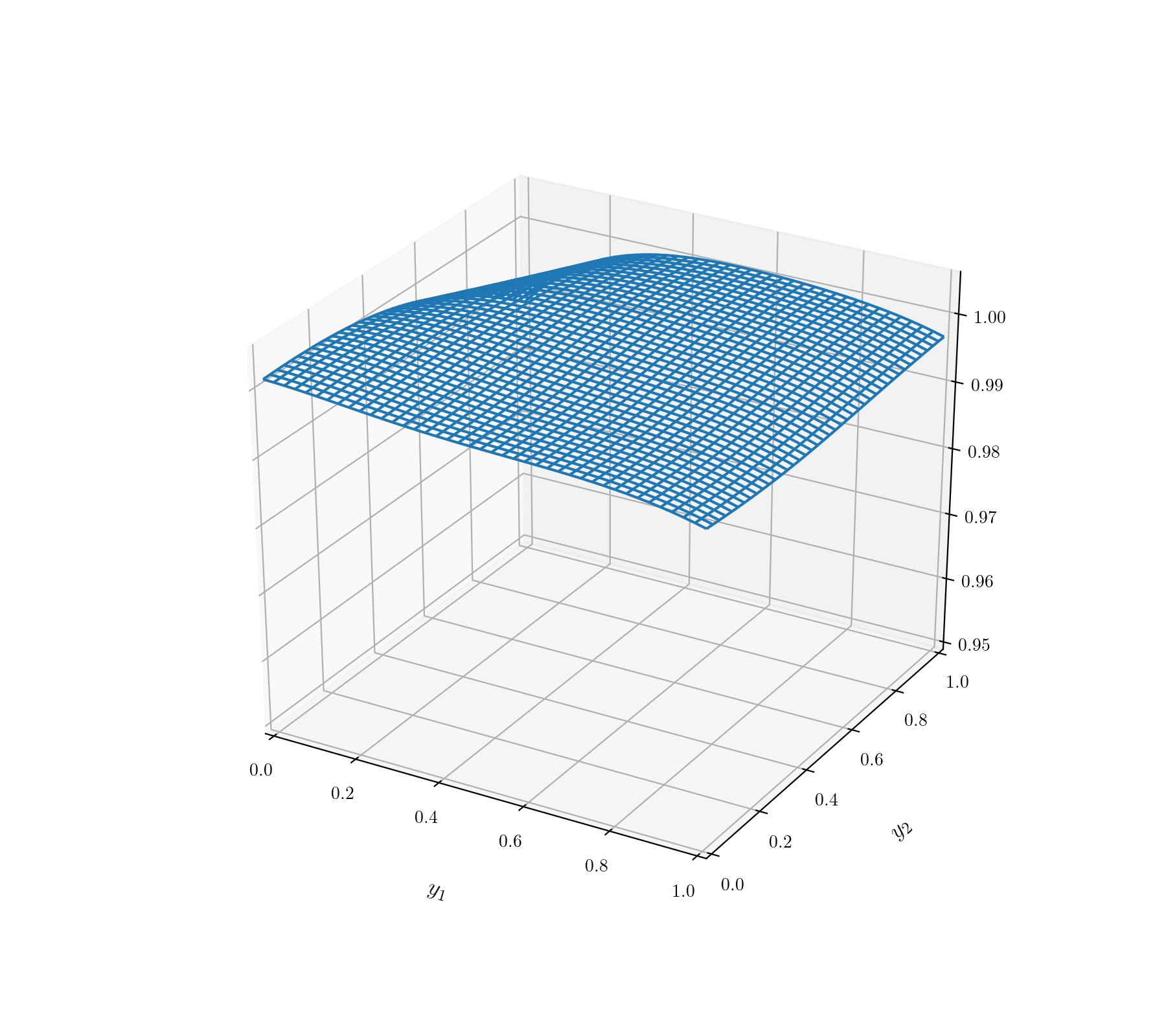
(d) $t=0.75T$

Figure 1: Surface of solution by the Deep Galerkin method. $(p=0.0005)$

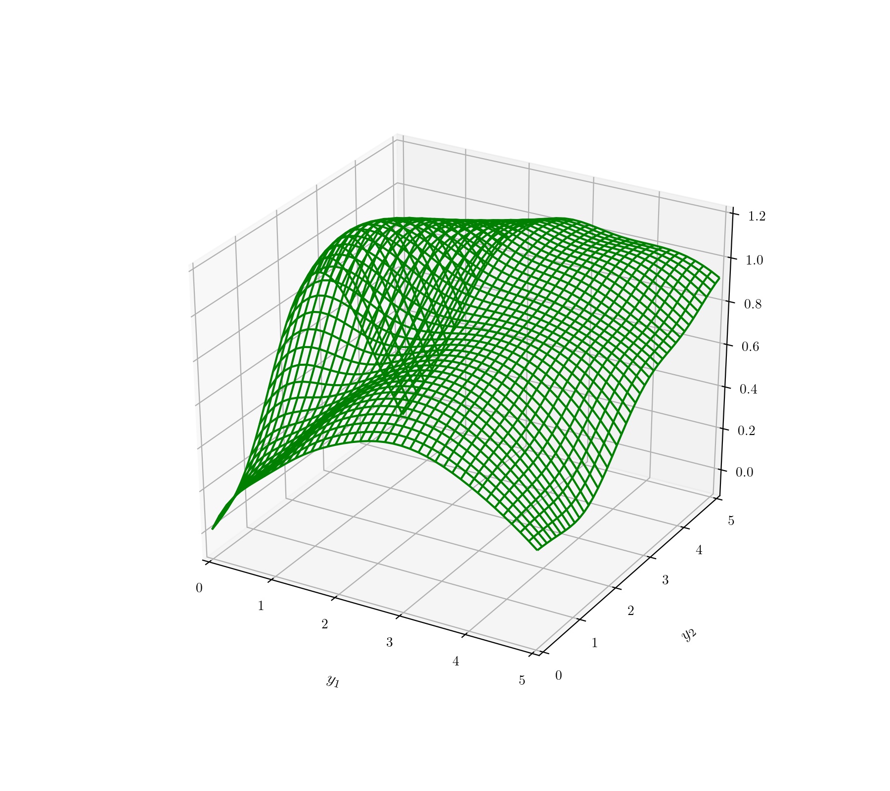
(a) $t=0$

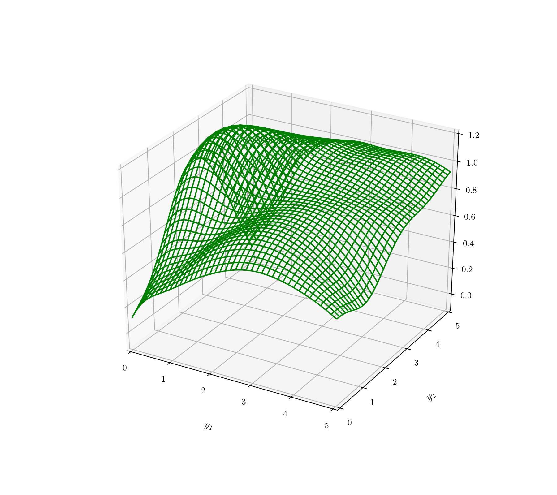
(b) $t=0.25T$

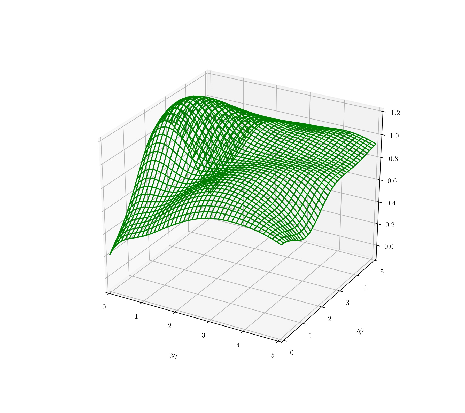
(c) $t=0.5T$

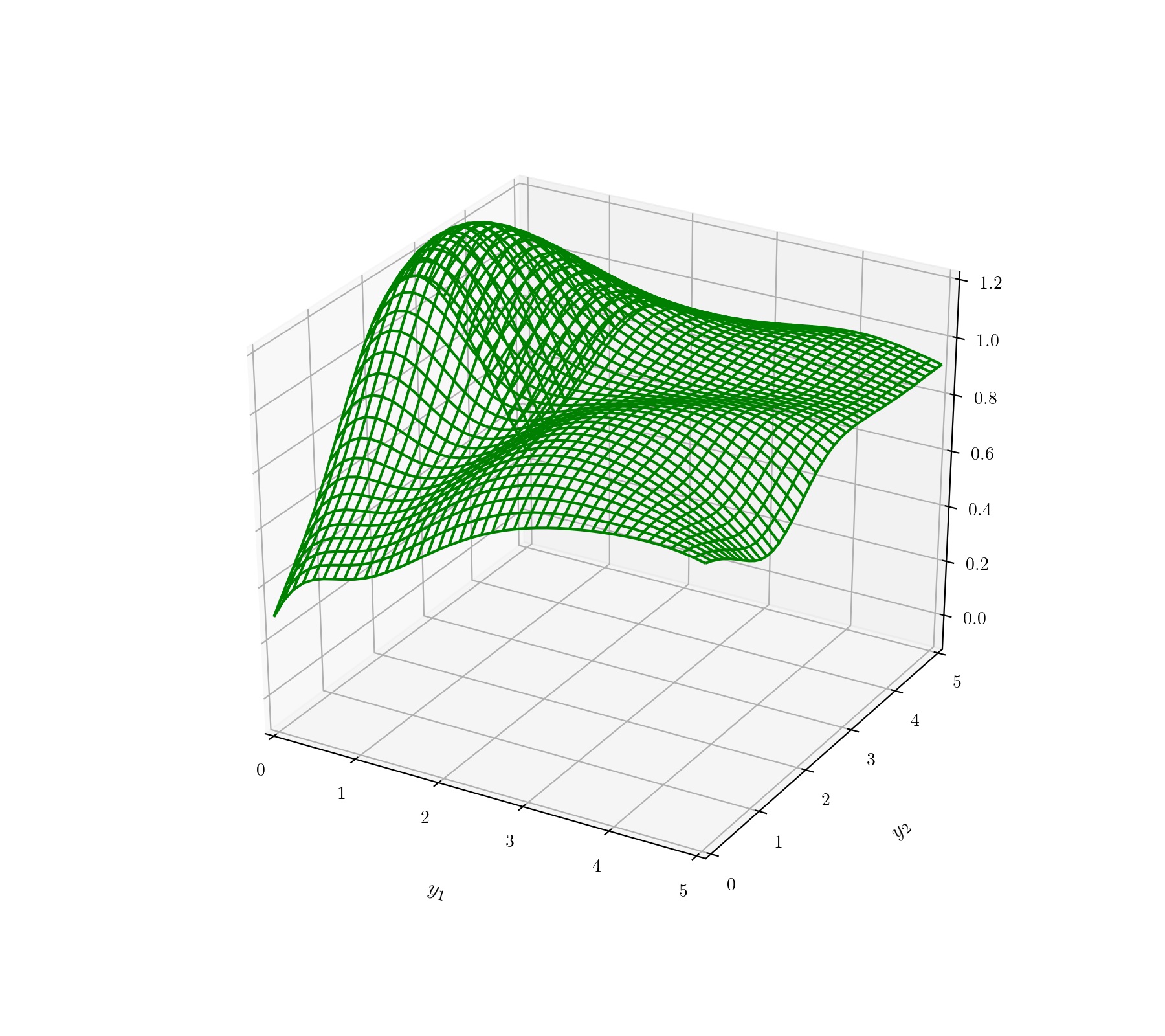
(d) $t=0.75T$

Figure 2: Surface of solution by the Deep Galerkin method. $(p=0.5)$

After solving (2.19) by the DGM algorithm, investors can choose their states $(y_{1},y_{2})\in[-10,10]\times[0,10]$ for fixed $t\in[0,T]$. The optimal portfolio can be constructed using (2.20) as:

$$\pi_{DGM}(t,\,y_{1},\,y_{2})=\dfrac{1}{1-p}\left(\Sigma^{-1}\mu+\Sigma^{-1}\Upsilon(\nabla_{y}u_{DGM})\dfrac{1}{u_{DGM}}\right).$$ (4.9)

To sum up, one can get the value of $u$ and the portfolio value $\pi$ at every time or state. The investor could buy or sell a risky asset $S^{(1)}$ based on the value of the portfolio to maximize utility from terminal wealth.

Figure 1 shows surfaces of the solution $u_{\text{DGM}}$ of (2.19) using DGM algorithm in different times, with the power utility preference parameter $p=0.0005$. We chose some part of domain $[0,1]\times[0,1]$ as a plot range for convenience. Figure 2 shows surfaces of the solution of (2.19) in $p=0.5$, with the restricted plot range $[0,5]\times[0,5]$. In both figures, for different values of utility parameter $p$, we can easily notice the fact that the surface tends to the plane $u=1$ as time goes to the terminal time $T$: the terminal condition of (2.19). Note however Figure 1 is more regular than Figure 2 in the sense that the value of $L^{2}$-loss in $p=0.0005$ was remarkably smaller than that in $p=0.5$. Hence we may infer the value of market preference parameter $p$ has played a significant role for using the Deep Galerkin method algorithm.

4.4 Comparing with the Finite Difference Method

Now we solve (2.19) using the finite difference method(FDM). The domain has equally divided $40$ grids satisfying:

$$0 =t^{0}<t^{1}<\cdots<t^{40}=T,$$ (4.10)

$$-10 =y_{1}^{0}<y_{1}^{1}<\cdots<y_{1}^{40}=10,$$

$$0 =y_{2}^{0}<y_{2}^{1}<\cdots<y_{2}^{40}=10.$$

First of all, we discretize the solution $u$ as

$$u_{i,j}^{n}:=u(t^{n},y_{1}^{i},y_{2}^{j}),\quad 0\leq i,j,n\leq 40.$$ (4.11)

With this notation, we can substitute the equation (2.19) using the following central difference formula:

$$u_{t}=\dfrac{u_{i,j}^{n+1}-u_{i,j}^{n}}{\Delta t},\quad u_{y_{1}}=\dfrac{u_{i+1,j}^{n}-u_{i-1,j}^{n}}{2(\Delta y_{1})},\quad u_{y_{2}}=\dfrac{u_{i,j+1}^{n}-u_{i,j-1}^{n}}{2(\Delta y_{2})}.$$ (4.12)

Note that we used the forward difference for discretizing $u_{t}$ in order to get the values of $(u_{i,j}^{n})_{1\leq i,j\leq 40}$ by using the values of $(u_{i,j}^{n+1})_{1\leq i,j\leq 40}$, for $n=0,\ldots,39$.

Also the central difference approximations of the second derivative of $u$ are given by:

$$u_{y_{1}y_{1}}=\dfrac{u_{i+1,j}^{n}-2u_{i,j}^{n}+u_{i-1,j}^{n}}{(\Delta y_{1})^{2}},\quad u_{y_{2}y_{2}}=\dfrac{u_{i,j+1}^{n}-2u_{i,j}^{n}+u_{i,j-1}^{n}}{(\Delta y_{2})^{2}},$$ (4.13)

$$u_{y_{1}y_{2}}=\dfrac{u_{i+1,j+1}^{n}-u_{i+1,j-1}^{n}-u_{i-1,j+1}^{n}+u_{i-1,j-1}^{n}}{4(\Delta y_{1})(\Delta y_{2})}.$$ (4.14)

Then the PDE (2.19) becomes a nonlinear equation with $1521$(=39$\times$39) unknowns $(u^{n}_{i,j})_{1\leq i,j\leq 39}$ for each $n=0$,$\ldots$,$39$. The equation is of the form:

$$\begin{split}&\dfrac{u_{i,j}^{n+1}-u_{i,j}^{n}}{\Delta t}+C_{1}\,\dfrac{u_{i+1,j}^{n}-u_{i-1,j}^{n}}{2(\Delta y_{1})}+C_{2}\,\dfrac{u_{i,j+1}^{n}-u_{i,j-1}^{n}}{2(\Delta y_{2})}+C_{3}\,\dfrac{u_{i+1,j}^{n}-2u_{i,j}^{n}+u_{i-1,j}^{n}}{(\Delta y_{1})^{2}}\\ &+C_{4}\,\dfrac{u_{i+1,j+1}^{n}-u_{i+1,j-1}^{n}-u_{i-1,j+1}^{n}+u_{i-1,j-1}^{n}}{4(\Delta y_{1})(\Delta y_{2})}+C_{5}\,\dfrac{u_{i,j+1}^{n}-2u_{i,j}^{n}+u_{i,j-1}^{n}}{(\Delta y_{2})^{2}}+C_{6}u_{i,j}^{n}\\ &-\dfrac{q}{2u_{i,j}^{n}}\left[C_{7}\left(\dfrac{u_{i+1,j}^{n}-u_{i-1,j}^{n}}{2(\Delta y_{1})}\right)^{2}+C_{8}\dfrac{u_{i+1,j}^{n}-u_{i-1,j}^{n}}{2(\Delta y_{1})}\dfrac{u_{i,j+1}^{n}-u_{i,j-1}^{n}}{2(\Delta y_{2})}+C_{9}(\dfrac{u_{i,j+1}^{n}-u_{i,j-1}^{n}}{2(\Delta y_{2})})^{2}\right]=0,\end{split}$$ (4.15)

where $C_{1},\ldots,C_{9}$ are constants. Note that the terminal condition $u(T,y)=u(T,y_{1},y_{2})=1$ also becomes

$$u^{40}_{i,j}=1\quad\text{for all}\quad 0\leq i,j\leq 40.$$ (4.16)

Since (2.19) has no boundary condition, we used the boundary data from the DGM algorithm. Figure 3 shows surfaces of the solution of (4.15) using the finite difference method in different times with $p=0.0005$. We used the Newton’s method since the equation (4.15) is nonlinear. For more detail, see Remani (2013).

(a) $t=0$

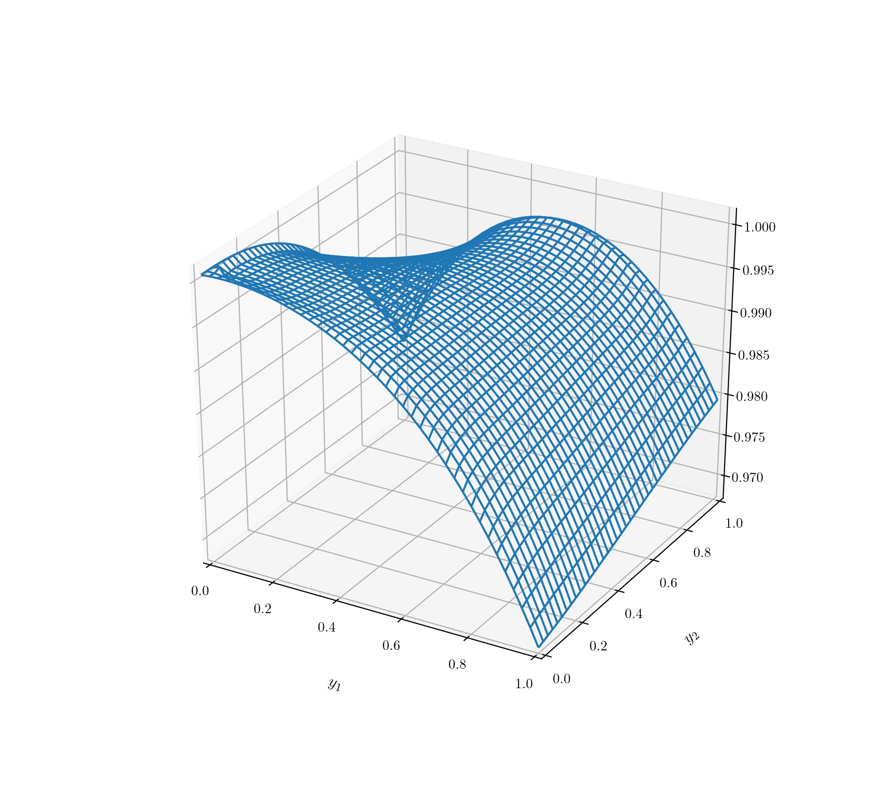
(b) $t=0.25T$

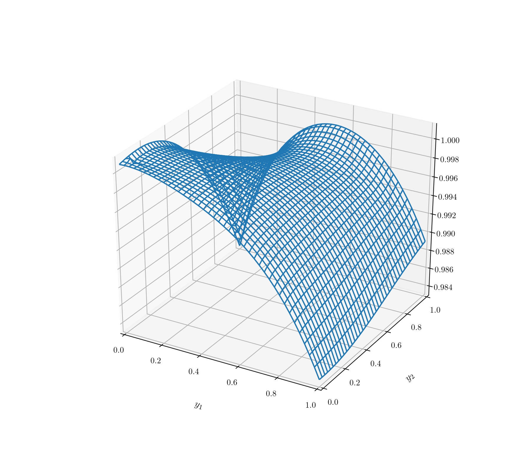
(c) $t=0.5T$

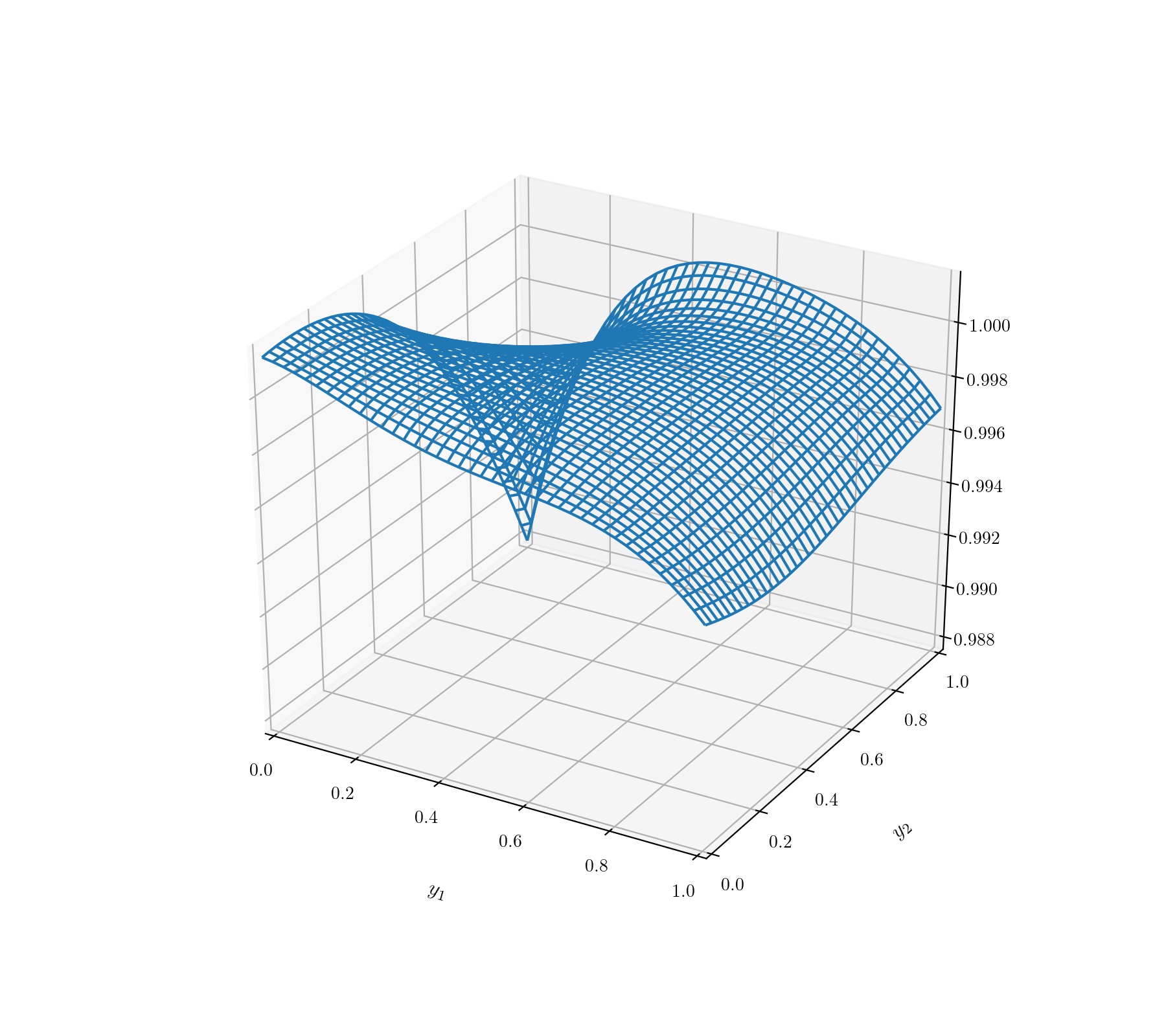
(d) $t=0.75T$

Figure 3: Surface of solution using the finite difference method

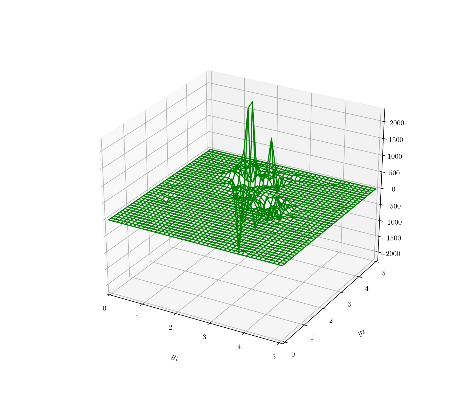
(a) $t=0$

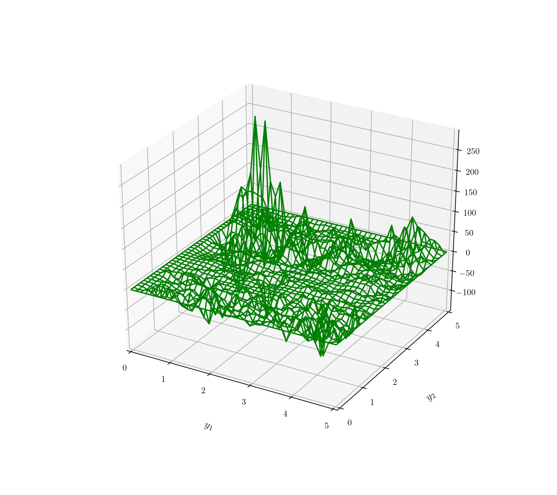
(b) $t=0.25T$

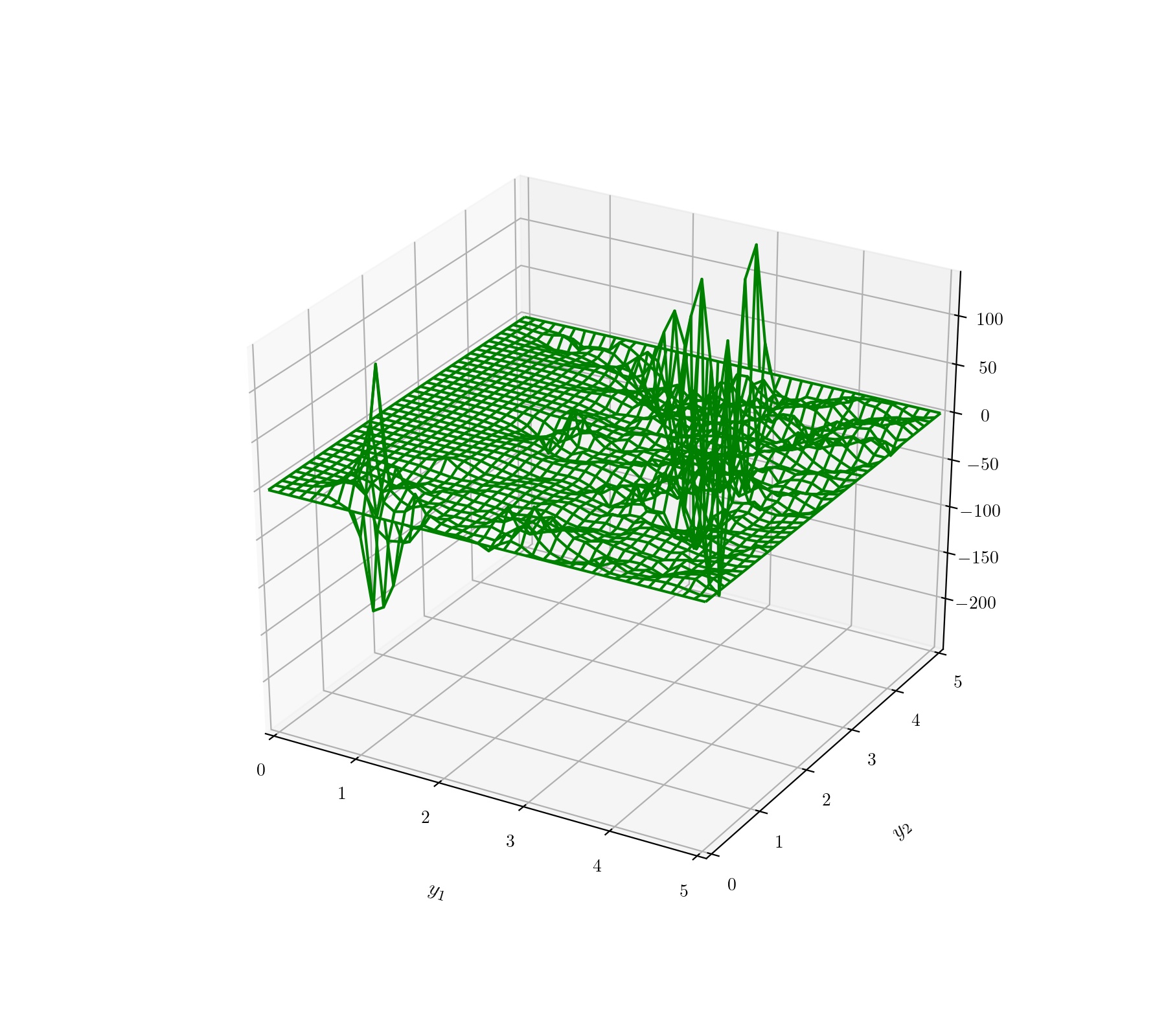
(c) $t=0.5T$

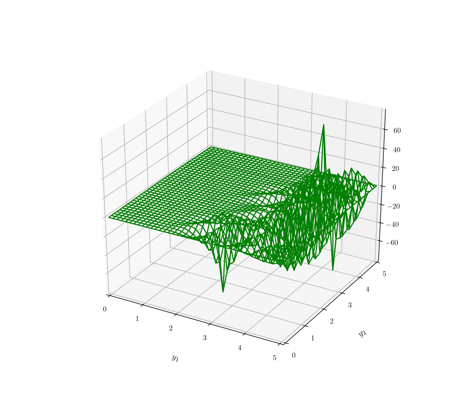
(d) $t=0.75T$

Figure 4: Surface of solution by the finite difference method $(p=0.5)$

With the same value of $p$, the absolute errors between the solution from the Deep Galerkin method and the one from the finite difference method are displayed in Figure 5. Notice that the error between these algorithms is getting slightly larger as the time $t$ goes to zero. This may be due to the time-reversely performed finite difference method algorithm, from $t=T$ to $t=0$. In other words, the stability on the solution from the terminal condition was gradually weakened as the time goes to zero.

In a different point of view, combining Figure 5 with Figure 1 and Figure 3, we conclude the solution is well-estimated by the deep neural network. It usually takes about $5$ minutes to train the network. On the other hand, it only takes less than $30$ seconds to find the surface of solution by the FDM. One can deduce this traditional algorithm would be more efficient for time-saving. However, it is not always true. Figure 4 shows surfaces derived from the finite difference method algorithm with $p=0.5$, same domain with Figure 2. In Figure 4, the solution has extremely large or small values. This singularity may have arised since the system of equations (4.15) is nonlinear. In other words, the matter of finding inverse matrix in the Newton’s method at each step $n=39,\ldots,0$ would make the value of solutions undesirable.

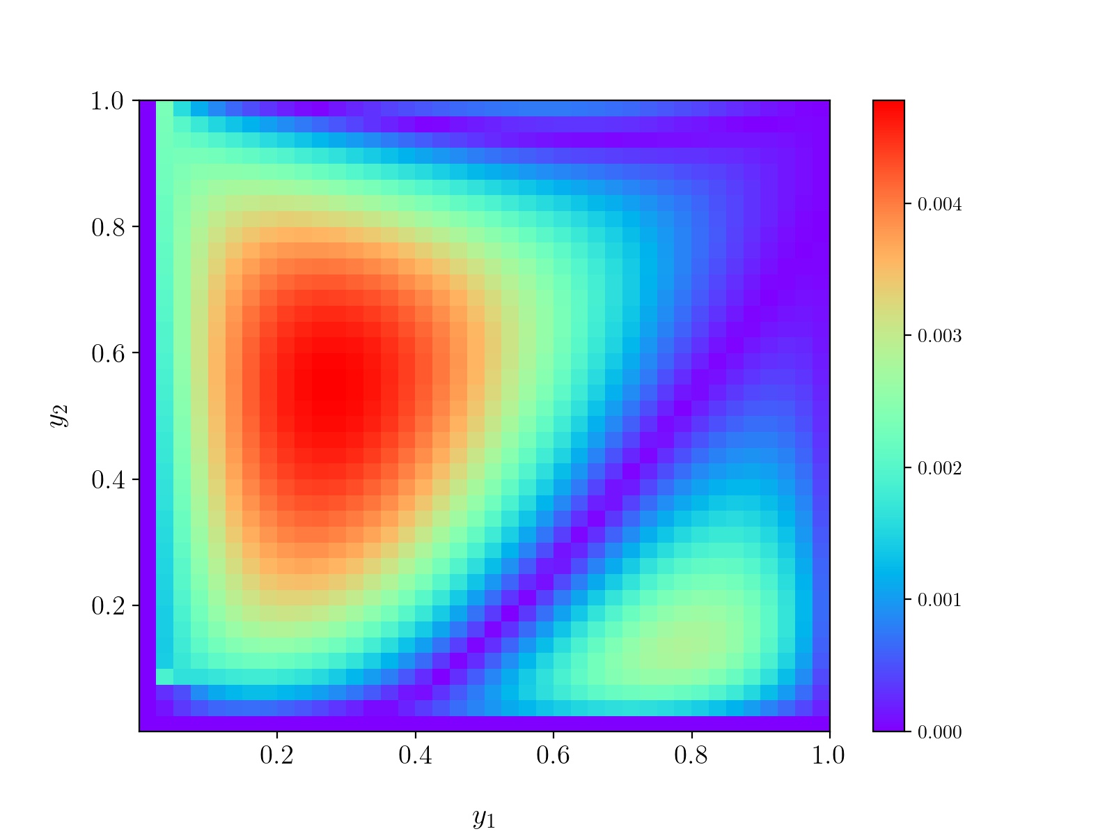
(a) $t=0$

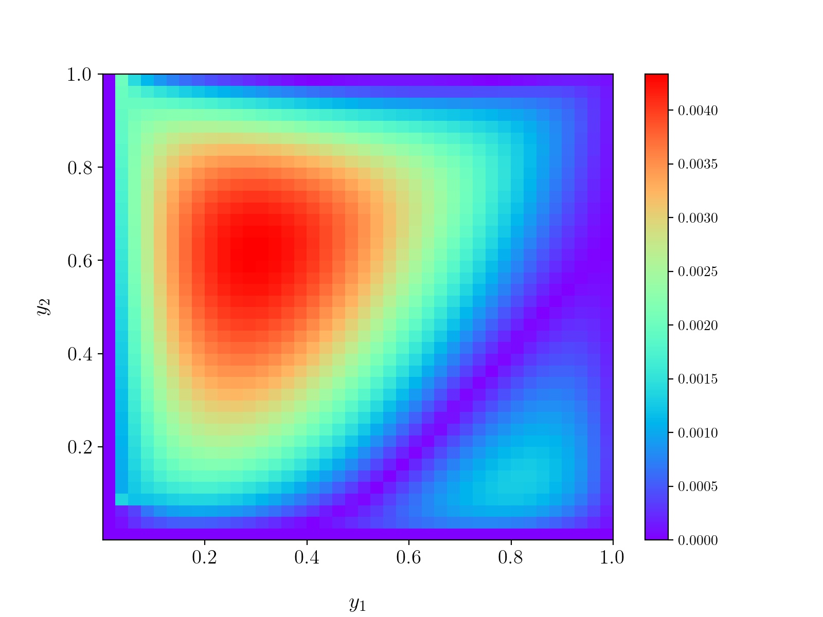
(b) $t=0.25T$

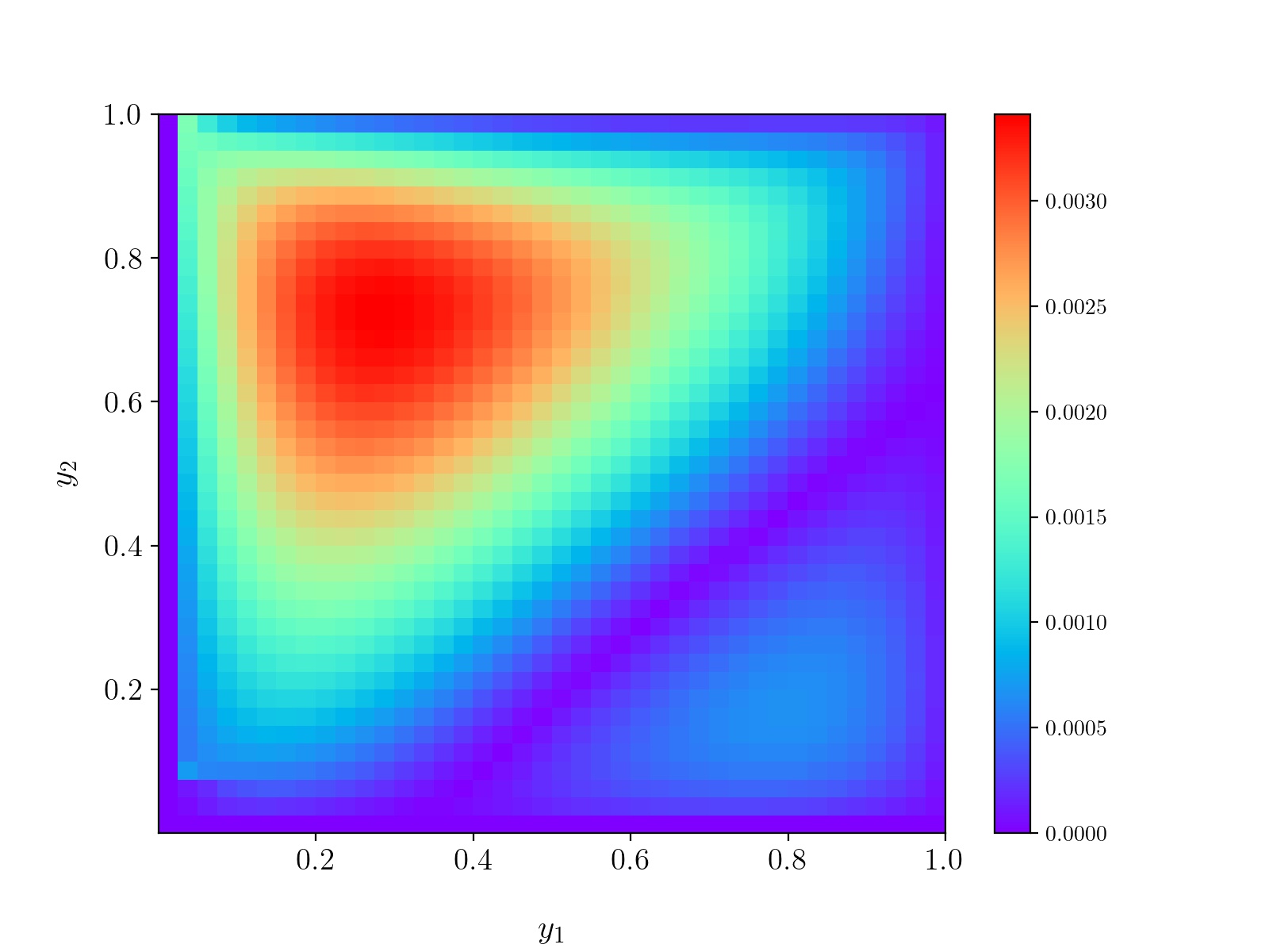
(c) $t=0.5T$

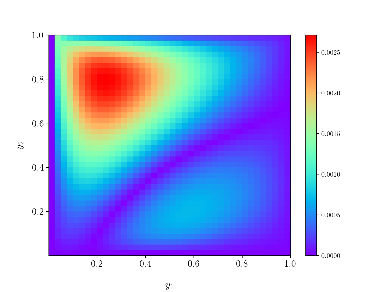
(d) $t=0.75T$

Figure 5: Absolute errors between the Deep Galerkin method and the finite difference method

5 Conclusion

In this paper we first modeled the market with a safe asset and some risky assets whose dynamics satisfy the diffusion process with returns. We then induced the HJB equation to maximize the expectation of an investor’s utility, given by investment opportunities modeled by a $d$-dimensional state process. Using some properties including homotheticity and concaveness, we finally derived a nonlinear partial differential equation and approximated the solution with a deep learning algorithm.

For comparison with the Deep Galerkin method, we applied the finite difference method to find an approximated solution. In case of the utility parameter being quite small, $p=0.0005$, we found that the solution has estimated well by the neural network. However in the case of $p=0.5$, there were several singular points in solution surfaces approximated by the finite difference method. Hence unlike the Deep Galerkin method, this mesh-based algorithm showed some defects such as a singularity by a nonlinearity of discretized version of partial differential equations. This concludes that the DGM algorithm is relatively stable and has less difficulties to approximate the solution for PDEs.

Furthermore, all above procedures in section 4 were performed only with the $2$-dimensional state process. If the dimension $d$ of state process increases, since there would exist millions of grids, it would be more computationally efficient to apply the DGM algorithm than the FDM algorithm. Finally with the approximated solution from the relatively stable DGM algorithm, the investor can decide how to allocate one’s wealth in several risky assets by the optimal portfolio formula.

Also there has some further studies to be researched. the stability or regularity of the solution is to be researched as the following are changed: model or dimension of a state variable $Y$, value of calibrated parameters, market preference parameter $p$ and sampling domain. Also in the optimal portfolio formula, the stability on a gradient term needs to be considered. Meanwhile, Sirignano and Spiliopoulos (2018) proved the convergence of the DGM algorithm only in a class of quasilinear parabolic PDEs. Although Sirignano and Spiliopoulos (2018) refered that the algorithm can be applied to other types of PDEs, there needs to be some researches for the stability of hyperbolic, elliptic or fully nonlinear PDEs.

Appendix A Proof of Theorem 3.1

Here we now justify Theorem 3.1 by proving the following two theorems in special cases. The main idea of proofs are from Sirignano and Spiliopoulos (2018) and Hornik (1991) based on universal approximation arguments. Note that the formulations in this section are not the same as the ones from the above papers. For completeness, we display almost all computations in the following proofs. The first theorem shows the convergence of $J(f)$: there exists a deep neural network $f$ such that the loss functional $J(f)$ tends to the arbitrary small. The latter one stands for the convergence of the DNN function to the solution of PDEs.

A.1 Convergence of the loss functional

Assume $D\subset\mathbb{R}^{d}$ is bounded with a smooth boundary $\partial D$. Denote $D_{T}=[0,T)\times D$. Consider the following form of quasilinear parabolic PDE:

$$\mathcal{G}[u](t,y):=\partial_{t}u(t,y)-\text{div}(\alpha(t,y,u,\nabla u))+\gamma(t,y,u,\nabla u) =0, (t,y)\in D_{T},$$ (A.1)

$$u(T,y) =u_{T}(y), y\in D.$$

Then the above differential operator $\mathcal{G}$ can be expressed as

$$\begin{split}\mathcal{G}[u](t,y)&=\partial_{t}u(t,y)-\sum_{i,j=1}^{d}\dfrac{\partial\alpha_{i}}{\partial u_{y_{j}}}\dfrac{\partial u_{y_{j}}}{\partial y_{i}}-\sum_{i=1}^{d}\dfrac{\partial\alpha_{i}}{\partial u}\partial_{y_{i}}u-\sum_{i=1}^{d}\dfrac{\partial\alpha_{i}}{\partial_{y_{i}}}+\gamma(t,y,u,\nabla u)\\ &=:\partial_{t}u(t,y)-\sum_{i,j=1}^{d}\dfrac{\partial\alpha_{i}}{\partial u_{y_{j}}}\dfrac{\partial u_{y_{j}}}{\partial y_{i}}+\hat{\gamma}(t,y,u,\nabla u).\end{split}$$ (A.2)

Theorem A.1.

Let $\mathfrak{C}^{n}(\psi)$ be a collection of DNN functions with $n$ hidden neurons in a single hidden layer:

$$\mathfrak{C}^{n}(\psi)=\left\{\zeta:\mathbb{R}^{1+d}\rightarrow\mathbb{R}:\zeta(t,y)=\sum_{i=1}^{n}\beta_{i}\psi\left(\alpha_{1i}t+\sum_{j=1}^{d}\alpha_{ji}y_{j}\right)+c_{i}\right\},$$ (A.3)

where $\psi$ is an activation function and $\theta=\left(\beta_{1},\cdots,\beta_{n},\alpha_{11},\cdots,\alpha_{dn},c_{1},\cdots,c_{n}\right)\in\mathbb{R}^{2n+n(1+d)}$ is a vector of the neural network parameters. Assume the following:

• $\psi$ is in $C^{2}(\mathbb{R}^{d})$, bounded and non-constant.

• $[0,T]\times D$ is compact.

• $\text{supp}\,\nu_{1}\subset D_{T}$ and $\text{supp}\,\nu_{2}\subset D$.

• The above PDE (A.1) has a unique solution, where this solution belongs to both $C(\bar{D}_{T})$ and $C^{1+\frac{\eta}{2},2+\eta}(D_{T})$ for $0\leq\eta\leq 1$, and

  $$\sup_{D_{T}}\left(\left|\nabla_{y}u(t,y)\right|+\left|\nabla_{y}^{2}u(t,y)\right|\right)<\infty.$$ (A.4)

• $\hat{\gamma}(t,y,u,p)$ and $\frac{\partial\alpha_{i}(t,y,u,p)}{\partial p_{j}}$ for $1\leq i,j\leq d$ are locally Lipschitz continuous, where Lipschitz constant has a polynomial growth in $u$ and $p$.

• $\dfrac{\partial\alpha_{i}(t,y,u,p)}{\partial u_{y_{j}}}$ is bounded, for $1\leq i,j\leq d$.

Then there is a constant

$$K=K\left(\sup\limits_{D_{T}}\left|u\right|,\,\sup\limits_{D_{T}}\left|\nabla_{y}u\right|,\,\sup\limits_{D_{T}}|\nabla_{y}^{2}u|\right)>0,$$ (A.5)

such that for arbitrary positive $\epsilon>0$, there is a DNN function $f$ in $\mathfrak{C}(\psi)=\bigcup\limits_{n=1}^{\infty}\mathfrak{C}^{n}(\psi)$ satisfying $J(f)\leq K\epsilon$.

Proof.

By Theorem 3 in Hornik (1991), for every $\epsilon>0$ and $u\in C^{1,2}([0,T]\times\mathbb{R}^{d})$, there is a DNN function $f=f(t,y;\theta)$ in $\mathfrak{C}(\psi)$ such that

$$\sup_{D_{T}}|\partial_{t}u-\partial_{t}f|\,+\sup_{\bar{D}_{T},0\leq j\leq 2}|\partial_{y}^{(j)}u-\partial_{y}^{(j)}f|<\epsilon.$$ (A.6)

Also we may assume for $C>0$, nonnegative constants $c_{1},c_{2},c_{3}$ and $c_{4}$,

$$|\hat{\gamma}(t,y,u,p)-\hat{\gamma}(t,y,v,q)|\leq C\left(|u|^{\frac{c_{1}}{2}}+|v|^{\frac{c_{2}}{2}}+|p|^{\frac{c_{3}}{2}}+|q|^{\frac{c_{4}}{2}}+1\right)(|u-v|+|p-q|),$$ (A.7)

by the local Lipschitz continuity of $\hat{\gamma}(t,y,u,p)$ in $u$ and $p$. We abbreviate $u(t,y)$ and $f(t,y;\theta)$ for convenience. From the Hölder inequality with exponents $r_{1}$ and $r_{2}$,

$\displaystyle\int_{D_{T}}|\hat{\gamma}(t,y,f,\nabla_{y}f)-\hat{\gamma}(t,y,u,\nabla_{y}u)|^{2}\,d\nu_{1}$

$\leq C\displaystyle\int_{D_{T}}(|f|^{c_{1}}+|u|^{c_{2}}+|\nabla_{y}f|^{c_{3}}+|\nabla_{y}u|^{c_{4}}+1)(|f-u|^{2}+|\nabla_{y}f-\nabla_{y}u|^{2})\,d\nu_{1}$

$\leq C\left(\displaystyle\int_{D_{T}}(|f|^{c_{1}}+|u|^{c_{2}}+|\nabla_{y}f|^{c_{3}}+|\nabla_{y}u|^{c_{4}}+1)^{r_{1}}\,d\nu_{1}\right)^{\frac{1}{r_{1}}}$

$\quad\times\left(\displaystyle\int_{D_{T}}(|f-u|^{2}+|\nabla_{y}f-\nabla_{y}u|^{2})^{r_{2}}\,d\nu_{1}\right)^{\frac{1}{r_{2}}}$

$\leq C\left(\displaystyle\int_{D_{T}}(|f-u|^{c_{1}}+|\nabla_{y}f-\nabla_{y}u|^{c_{3}}+|u|^{c_{1}\vee c_{2}}+|\nabla_{y}u|^{c_{3}\vee c_{4}}+1)^{r_{1}}\,d\nu_{1}\right)^{\frac{1}{r_{1}}}$

$\quad\times\left(\displaystyle\int_{D_{T}}(|f-u|^{2}+|\nabla_{y}f-\nabla_{y}u|^{2})^{r_{2}}\,d\nu_{1}\right)^{\frac{1}{r_{2}}}$

$\leq C\left(\epsilon^{c_{1}}+\epsilon^{c_{3}}+\sup\limits_{D_{T}}|u|^{c_{1}\vee c_{2}}+\sup\limits_{D_{T}}|\nabla_{y}u|^{c_{3}\vee c_{4}}\right)\epsilon^{2}$.

Each constant $C$ from the above inequalities may differ from each other. The last inequality holds because of (A.6).

Also we may assume

$$\left|\dfrac{\partial\alpha_{i}(t,y,u,p)}{\partial p_{j}}-\dfrac{\partial\alpha_{i}(t,y,v,q)}{\partial q_{j}}\right|\leq C\left(|u|^{\frac{c_{1}}{2}}+|v|^{\frac{c_{2}}{2}}+|p|^{\frac{c_{3}}{2}}+|q|^{\frac{c_{4}}{2}}+1\right)(|u-v|+|p-q|),$$ (A.8)

by the local Lipschitz continuity of $\frac{\partial\alpha_{i}(t,y,u,p)}{\partial p_{j}}$ in $u$ and $p$. For convenience, we denote

$$\xi(t,y,h,\nabla h,\nabla^{2}h)=\sum_{i,j=1}^{d}\dfrac{\partial\alpha_{i}(t,y,h,\nabla h)}{\partial h_{y_{j}}}\partial_{{y_{i}}{y_{j}}}h(t,y).$$ (A.9)

In spirit to the above procedure we used the Hölder inequality with exponents $p$ and $q$:

$\displaystyle\int_{D_{T}}|\xi(t,y,u,\nabla_{y}u,\nabla_{y}^{2}u)-\xi(t,y,f,\nabla_{y}f,\nabla_{y}^{2}f)|^{2}\,d\nu_{1}$

$\leq\displaystyle\int_{D_{T}}\left|\sum_{i,j=1}^{d}\left(\dfrac{\partial\alpha_{i}(t,y,f,\nabla f)}{\partial f_{y_{j}}}-\dfrac{\partial\alpha_{i}(t,y,u,\nabla u)}{\partial u_{y_{j}}}\right)\partial_{{y_{i}}{y_{j}}}u(t,y)\right|^{2}\,d\nu_{1}$

$\quad+\displaystyle\int_{D_{T}}\left|\sum_{i,j=1}^{d}\dfrac{\partial\alpha_{i}(t,y,f,\nabla f)}{\partial f_{y_{j}}}(\partial_{{y_{i}}{y_{j}}}f(t,y;\theta)-\partial_{{y_{i}}{y_{j}}}u(t,y))\right|^{2}\,d\nu_{1}$

$\leq C\displaystyle\sum_{i,j=1}^{d}\left(\displaystyle\int_{D_{T}}|\partial_{{y_{i}}{y_{j}}}u(t,y)|^{2p}\,d\nu_{1}\right)^{\frac{1}{p}}\left(\displaystyle\int_{D_{T}}\left|\dfrac{\partial\alpha_{i}(t,y,f,\nabla f)}{\partial f_{y_{j}}}-\dfrac{\partial\alpha_{i}(t,y,u,\nabla u)}{\partial u_{y_{j}}}\right|^{2q}\,d\nu_{1}\right)^{\frac{1}{q}}$

$\quad+\,C\displaystyle\sum_{i,j=1}^{d}\left(\displaystyle\int_{D_{T}}\left|\dfrac{\partial\alpha_{i}(t,y,f,\nabla f)}{\partial f_{y_{j}}}\right|^{2p}\,d\nu_{1}\right)^{\frac{1}{p}}\left(\displaystyle\int_{D_{T}}|\partial_{{y_{i}}{y_{j}}}f(t,y;\theta)-\partial_{{y_{i}}{y_{j}}}u(t,y)|^{2q}\,d\nu_{1}\right)^{\frac{1}{q}}$

$\leq C\displaystyle\sum_{i,j=1}^{d}\left(\displaystyle\int_{D_{T}}|\partial_{{y_{i}}{y_{j}}}u(t,y)|^{2p}\,d\nu_{1}\right)^{\frac{1}{p}}\left(\displaystyle\int_{D_{T}}(|f-u|^{2}+|\nabla_{y}f-\nabla_{y}u|^{2})^{qr_{2}}\,d\nu_{1}\right)^{\frac{1}{qr_{2}}}$

$\quad\times\left(\displaystyle\int_{D_{T}}(|f-u|^{c_{1}}+|\nabla_{y}f-\nabla_{y}u|^{c_{3}}+|u|^{c_{1}\vee c_{2}}+|\nabla_{y}u|^{c_{3}\vee c_{4}}+1)^{qr_{1}}\,d\nu_{1}\right)^{\frac{1}{qr_{1}}}$

$\quad+\,C\displaystyle\sum_{i,j=1}^{d}\left(\displaystyle\int_{D_{T}}\left|\dfrac{\partial\alpha_{i}(t,y,f,\nabla f)}{\partial f_{y_{j}}}\right|^{2p}\,d\nu_{1}\right)^{\frac{1}{p}}\left(\displaystyle\int_{D_{T}}|\partial_{{y_{i}}{y_{j}}}f(t,y;\theta)-\partial_{{y_{i}}{y_{j}}}u(t,y)|^{2q}\,d\nu_{1}\right)^{\frac{1}{q}}$

$\leq C\epsilon^{2}$.

To sum up, we finally obtain the following inequality:

$$J(f) =\lVert\mathcal{G}[f]\rVert^{2}_{D_{T},\nu_{1}}+\lVert f(T,y;\theta)-u_{T}(y)\rVert^{2}_{D,\nu_{2}}$$ (A.10)

$$=\lVert\mathcal{G}[f]-\mathcal{G}[g]\rVert^{2}_{D_{T},\nu_{1}}+\lVert f(T,y;\theta)-u_{T}(y)\rVert^{2}_{D,\nu_{2}}$$

$$\leq\int_{D_{T}}\left(|\partial_{t}u-\partial_{t}f|^{2}+|\xi(t,y,u,\nabla u,\nabla^{2}u)-\xi(t,y,f,\nabla f,\nabla^{2}f)|^{2}\right)\,d\nu_{1}$$

$$\quad+\int_{D_{T}}|\hat{\gamma}(t,y,f,\nabla_{y}f)-\hat{\gamma}(t,y,u,\nabla_{y}u)|^{2}\,d\nu_{1}+\int_{D}|f(T,y;\theta)-u_{T}(y)|^{2}\,d\nu_{2}$$

$$\leq K\epsilon^{2}$$

for some constant $K>0$. ∎

A.2 Convergence of the DNN function to the solution of PDEs

As we done in section A.1, consider the quasilinear parabolic PDE (A.1) and the following loss functional

$$J(f)=\lVert\mathcal{G}[f]\rVert^{2}_{D_{T},\nu_{1}}+\lVert f(T,y;\theta)-u_{T}(y)\rVert^{2}_{D,\nu_{2}}.$$ (A.11)

By Theorem A.1, there is a neural network $f^{n}$ such that $J(f^{n})$ tends to $0$. Each $f^{n}$ satisfies the following:

$$\mathcal{G}[f^{n}](t,y) =h^{n}(t,y), (t,y)\in D_{T},$$ (A.12)

$$f^{n}(T,y) =u_{T}^{n}(y), y\in D,$$

and

$$\lVert h^{n}\rVert^{2}_{D_{T},\nu_{1}}+\lVert u_{T}^{n}-u_{T}\rVert^{2}_{D,\nu_{2}}\rightarrow 0\text{ as }n\rightarrow\infty.$$ (A.13)

Theorem A.2.

Assume the following:

• $\lVert\alpha(t,y,u,p)\rVert\leq\mu(\lVert p\rVert+\kappa(t,y))$ for all $(t,y)\in D_{T}$, with $\mu>0$ and $\kappa\in L^{2}(D_{T})$ being positive.

• $\alpha$ is continuously differentiable in $(y,u,p)$.

• Both $\alpha$ and $\gamma$ are Lipschitz continuous, uniformly on the following form of compact sets:

  $$\left\{(t,y,u,p):t\in[0,T],\,y\in\bar{D},\,0\leq|u|\leq C,\,0\leq\lVert p\rVert\leq C\right\}.$$ (A.14)

• $\left\langle p,\,\alpha(t,y,u,p)\right\rangle\geq\nu\lVert p\rVert^{2}$ for some $\nu>0$.

• $\left\langle p_{1}-p_{2},\,\alpha(t,y,u,p_{1})-\alpha(t,y,u,p_{2})\right\rangle>0$ for some $\nu>0$, for every $p_{1},p_{2}\in\mathbb{R}^{d}$ with $p_{1}\neq p_{2}$.

• $|\gamma(t,y,u,p)|\leq\lVert p\rVert\lambda(t,y)$ for all $(t,y)\in D_{T}$, with $\lambda\in L^{d+2}(D_{T})$ being positive.

• $u_{T}(y)\in C^{0,2+\xi}(\bar{D})$ for some $\xi>0$. Note that

  $$\lVert u(y)\rVert_{C^{0,\beta}(\bar{D})}=\sup_{y\in\bar{D}}|u(y)|^{[\beta]}+\sup_{y_{1},y_{2}\in\bar{D},y_{1}\neq y_{2}}\dfrac{|u(y_{1})-u(y_{2})|}{|y_{1}-y_{2}|^{\beta-[\beta]}}.$$ (A.15)

• $u_{T}$ and $u_{T}^{\prime}$ are bounded in $\bar{D}$.

• $D\subset\mathbb{R}^{d}$ is bounded and open with boundary $\partial D\in C^{2}$.

• $(f^{n})_{n\in\mathbb{N}}\in C^{1,2}(\bar{D}_{T})$ and $(f^{n})_{n\in\mathbb{N}}\in L^{2}(D_{T})$.

Then

1. the PDE (A.1) has a unique bounded solution

   $$u\in C^{0,\delta,\frac{\delta}{2}}(\bar{D}_{T})\cap W_{0}^{(1,2),2}(D_{T}^{\star})\cap L^{2}\left(0,T;W_{0}^{1,2}(D)\right),\quad\delta>0,$$ (A.16)

   for any interior subdomain $D_{T}^{\star}\subset D_{T}$.

2. $f^{n}\rightarrow u$ strongly in $L^{\rho}(D_{T})$ for every $\rho<2$.

Note that in case of the class of quasilinear parabolic PDEs with boundary conditions, we should also consider the limiting process in the weak formulation of PDEs and use the Vitali’s theorem. For more detail, see Appendix A in Sirignano and Spiliopoulos (2018). See also Boccardo et al. (2009), Magliocca (2018), Di Nardo et al. (2011) and Debnath (2011).

Proof.

Existence, regularity and uniqueness for (A.1) follows from Theorem 2.1 in Porzio (1999) and Theorem 6.3 to 6.5 of chapter V.6 in Ladyzhenskaia et al. (1968). Boundedness holds by Theorem 2.1 in Porzio (1999). See also chapter V.2 from Ladyzhenskaia et al. (1968).

Let $f^{n}$ be the solution of (A.12). By Lemma 4.1 of Porzio (1999), $\left\{f^{n}\right\}_{n\in\mathbb{N}}$ is uniformly bounded in both $L^{\infty}(0,T;L^{2}(D))$ and $L^{2}\left(0,T;W_{0}^{1,2}(D)\right)$. Then we can pick a subsequence from the sequence of neural networks $\left\{f^{n}\right\}_{n\in\mathbb{N}}$, where we denote also by $\left\{f^{n}\right\}_{n\in\mathbb{N}}$ for convenience, satisfying

• $f^{n}\xrightarrow{w*}u$ in $L^{\infty}(0,T;L^{2}(D))$,

• $f^{n}\rightarrow u$, weakly in $L^{2}\left(0,T;W_{0}^{1,2}(D)\right)$,

• $f^{n}(\cdot,t)\rightarrow v(\cdot,t)$, weakly in $L^{2}(D)$, for every fixed $t$ in $[0,T)$,

for some functions $u,v$. Since the norm of $f$ in a Banach space $L^{2}\left(0,T;W_{0}^{1,2}(D)\right)$ is defined as

$$\lVert f\rVert_{L^{2}\left(0,T;W_{0}^{1,2}(D)\right)}=\left(\displaystyle\int_{0}^{T}\lVert f\rVert_{W_{0}^{1,2}(D)}^{2}\,dt\right)^{\frac{1}{2}},$$ (A.17)

where

$$\lVert f\rVert_{W_{0}^{1,2}(D)}^{2}=\sum_{|\alpha|\leq 2}\lVert D^{\alpha}f\rVert_{L^{2}(D)}^{2}=\lVert f\rVert_{L^{2}(D)}^{2}+\lVert Df\rVert_{L^{2}(D)}^{2}+\lVert D^{2}f\rVert_{L^{2}(D)}^{2},$$ (A.18)

$\left\{\nabla_{y}f^{n}\right\}_{n\in\mathbb{N}}$ is uniformly bounded in $L^{2}(0,T;W_{0}^{1,2}(D))$.

Let $q=1+\dfrac{d}{d+4}\in(1,2)$. By the Hölder inequality with exponents $r_{1},r_{2}>1$,

$$\int_{D_{T}}\left|\gamma(t,y,f^{n},\nabla_{y}f^{n})\right|^{q}\,dtdy \leq\int_{D_{T}}|\lambda(t,y)|^{q}|\nabla_{y}f^{n}(t,y)|^{q}\,dtdy$$ (A.19)

$$\leq\left(\int_{D_{T}}|\lambda(t,y)|^{r_{1}q}\,dtdy\right)^{\frac{1}{r_{1}}}\left(\int_{D_{T}}|\nabla_{y}f^{n}(t,y)|^{r_{2}q}\,dtdy\right)^{\frac{1}{r_{2}}}.$$

Choose $r_{2}=\dfrac{2}{q}$. Then we get $r_{1}=\dfrac{2}{2-q}$ and hence $r_{1}q=d+2$. Since $\lambda\in L^{d+2}(D_{T})$ and $\left\{\nabla_{y}f^{n}\right\}_{n\in\mathbb{N}}$ is uniformly bounded,

$$\int_{D_{T}}\left|\gamma(t,y,f^{n},\nabla_{y}f^{n})\right|^{q}\,dtdx\leq C,$$ (A.20)

for some $C>0$.

The growth assumption on $\alpha$ and the above argument imply that $\left\{\partial_{t}f^{n}\right\}_{n\in\mathbb{N}}$ is uniformly bounded in $L^{1+\frac{d}{d+4}}(D_{T})$ and $L^{2}\left(0,T;W^{-1,2}(D)\right)$. Let $\delta_{1},\delta_{2}$ be the conjugate exponents satisfying $\delta_{2}>\max\left\{2,d\right\}$. By the Gagliardo–Nirenberg–Sobolev inequality and the Rellich–Kondrachov compactness theorem(for further details, see chapter 5 in Evans (2002)), the following embeddings hold:

$$W^{-1,2}(D)\subset W^{-1,\delta_{1}}(D),\quad L^{q}(D)\subset W^{-1,\delta_{1}}(D)\text{, and }L^{2}(D)\subset W^{-1,\delta_{1}}(D),$$ (A.21)

and hence $\left\{\partial_{t}f^{n}\right\}_{n\in\mathbb{N}}$ is uniformly bounded in $L^{1}(0,T;W^{-1,\delta_{1}}(D))$.

By Corollary 4 in Simon (1986) and the following embedding

$$W_{0}^{1,2}(D)\subset\subset L^{2}(D)\subset W^{-1,\delta_{1}}(D),$$ (A.22)

$\left\{f^{n}\right\}_{n\in\mathbb{N}}$ is relatively compact in $L^{2}(D_{T})$, in other words,

$$f^{n}\rightarrow u\text{ strongly in }L^{2}(D_{T})\text{ as }n\rightarrow\infty.$$ (A.23)

Thus

$$f^{n}\rightarrow u\text{ almost everywhere in }D_{T}\text{ up to subsequences.}$$ (A.24)

Note that from the Theorem 3.3 of Boccardo et al. (1997), we get

$$\nabla f^{n}\rightarrow\nabla u\text{ almost everywhere in }D_{T}.$$ (A.25)

Hence $f^{n}\rightarrow u$ strongly in $L^{\rho}\left(0,T;W_{0}^{1,\rho}(D)\right)$ and so in $L^{\rho}(D_{T})$ for every $\rho<2$, by (A.24) and (A.25).

∎

Acknowledgement.
Hyungbin Park was supported by Research Resettlement Fund for the new faculty of Seoul National University. Hyungbin Park was also supported by the National Research Foundation of Korea (NRF) grants funded by the Ministry of Science and ICT (No. 2018R1C1B5085491 and No. 2017R1A5A1015626) and the Ministry of Education (No. 2019R1A6A1A10073437) through Basic Science Research Program.

References

• Achdou and Pironneau (2005) Achdou, Y. and Pironneau, O. (2005). Computational methods for option pricing. SIAM.
• Al-Aradi et al. (2018) Al-Aradi, A., Correia, A., Naiff, D., Jardim, G., and Saporito, Y. (2018). Solving nonlinear and high-dimensional partial differential equations via deep learning. arXiv preprint arXiv:1811.08782.
• Al-Aradi et al. (2019) Al-Aradi, A., Correia, A., Naiff, D. d. F., Jardim, G., and Saporito, Y. (2019). Applications of the deep galerkin method to solving partial integro-differential and hamilton-jacobi-bellman equations. arXiv preprint arXiv:1912.01455.
• Benth et al. (2003) Benth, F. E., Karlsen, K. H., and Reikvam, K. (2003). Merton’s portfolio optimization problem in a black and scholes market with non-gaussian stochastic volatility of ornstein-uhlenbeck type. Mathematical Finance: An International Journal of Mathematics, Statistics and Financial Economics, 13(2):215–244.
• Björk (2009) Björk, T. (2009). Arbitrage theory in continuous time. Oxford university press.
• Boccardo et al. (1997) Boccardo, L., Dall’Aglio, A., Gallouët, T., and Orsina, L. (1997). Nonlinear parabolic equations with measure data. journal of functional analysis, 147(1):237–258.
• Boccardo et al. (2009) Boccardo, L., Porzio, M. M., and Primo, A. (2009). Summability and existence results for nonlinear parabolic equations. Nonlinear Analysis: Theory, Methods & Applications, 71(3-4):978–990.
• Burden et al. (2010) Burden, R., Faires, J. D., and Reynolds, A. (2010). Numerical analysis, brooks/cole. Boston, Mass, USA,.
• Callegaro et al. (2017) Callegaro, G., Gaïgi, M., Scotti, S., and Sgarra, C. (2017). Optimal investment in markets with over and under-reaction to information. Mathematics and Financial Economics, 11(3):299–322.
• Crisóstomo (2014) Crisóstomo, R. (2014). An analyisis of the heston stochastic volatility model: Implementation and calibration using matlab.
• Danilova et al. (2010) Danilova, A., Monoyios, M., and Ng, A. (2010). Optimal investment with inside information and parameter uncertainty. Mathematics and Financial Economics, 3(1):13–38.
• Debnath (2011) Debnath, L. (2011). Nonlinear partial differential equations for scientists and engineers. Springer Science & Business Media.
• Di Nardo et al. (2011) Di Nardo, R., Feo, F., and Guibe, O. (2011). Existence result for nonlinear parabolic equations with lower order terms. Anal. Appl.(Singap.), 9(2):161–186.
• Evans (2002) Evans, L. C. (2002). Partial differential equations, ams. Graduate Studies in Mathematics, 19.
• Guasoni and Robertson (2015) Guasoni, P. and Robertson, S. (2015). Static fund separation of long-term investments. Mathematical Finance, 25(4):789–826.
• Han et al. (2018) Han, J., Jentzen, A., and Weinan, E. (2018). Solving high-dimensional partial differential equations using deep learning. Proceedings of the National Academy of Sciences, 115(34):8505–8510.
• Hansen (2013) Hansen, S. L. (2013). Optimal consumption and investment strategies with partial and private information in a multi-asset setting. Mathematics and Financial Economics, 7(3):305–340.
• Hornik (1991) Hornik, K. (1991). Approximation capabilities of multilayer feedforward networks. Neural networks, 4(2):251–257.
• Kühn and Stroh (2010) Kühn, C. and Stroh, M. (2010). Optimal portfolios of a small investor in a limit order market: a shadow price approach. Mathematics and Financial Economics, 3(2):45–72.
• Ladyzhenskaia et al. (1968) Ladyzhenskaia, O. A., Solonnikov, V. A., and Ural’tseva, N. N. (1968). Linear and quasi-linear equations of parabolic type, volume 23. American Mathematical Soc.
• Lagaris et al. (2000) Lagaris, I. E., Likas, A. C., and Papageorgiou, D. G. (2000). Neural-network methods for boundary value problems with irregular boundaries. IEEE Transactions on Neural Networks, 11(5):1041–1049.
• Lee and Kang (1990) Lee, H. and Kang, I. S. (1990). Neural algorithm for solving differential equations. Journal of Computational Physics, 91(1):110–131.
• Lemaire et al. (2020) Lemaire, V., Montes, T., et al. (2020). Stationary heston model: Calibration and pricing of exotics using product recursive quantization. arXiv preprint arXiv:2001.03101.
• Liang and Ma (2020) Liang, Z. and Ma, M. (2020). Robust consumption-investment problem under crra and cara utilities with time-varying confidence sets. Mathematical Finance, 30(3):1035–1072.
• Magliocca (2018) Magliocca, M. (2018). Existence results for a cauchy–dirichlet parabolic problem with a repulsive gradient term. Nonlinear Analysis, 166:102–143.
• Malek and Beidokhti (2006) Malek, A. and Beidokhti, R. S. (2006). Numerical solution for high order differential equations using a hybrid neural network—optimization method. Applied Mathematics and Computation, 183(1):260–271.
• Mehrdoust and Fallah (2020) Mehrdoust, F. and Fallah, S. (2020). On the calibration of fractional two-factor stochastic volatility model with non-lipschitz diffusions. Communications in Statistics-Simulation and Computation, pages 1–20.
• Merton (1969) Merton, R. C. (1969). Lifetime portfolio selection under uncertainty: The continuous-time case. The review of Economics and Statistics, pages 247–257.
• Nutz (2010) Nutz, M. (2010). The opportunity process for optimal consumption and investment with power utility. Mathematics and financial economics, 3(3-4):139–159.
• Pedersen and Peskir (2017) Pedersen, J. L. and Peskir, G. (2017). Optimal mean-variance portfolio selection. Mathematics and Financial Economics, 11(2):137–160.
• Porzio (1999) Porzio, M. M. (1999). Existence of solutions for some” noncoercive” parabolic equations. Discrete & Continuous Dynamical Systems-A, 5(3):553.
• Remani (2013) Remani, C. (2013). Numerical methods for solving systems of nonlinear equations. Lakehead University Thunder Bay, Ontario, Canada.
• Simon (1986) Simon, J. (1986). Compact sets in the space $L^{p}(0,T;B)$. Annali di Matematica pura ed applicata, 146(1):65–96.
• Sirignano and Spiliopoulos (2018) Sirignano, J. and Spiliopoulos, K. (2018). Dgm: A deep learning algorithm for solving partial differential equations. Journal of computational physics, 375:1339–1364.
• Weinan et al. (2019) Weinan, E., Hutzenthaler, M., Jentzen, A., and Kruse, T. (2019). On multilevel picard numerical approximations for high-dimensional nonlinear parabolic partial differential equations and high-dimensional nonlinear backward stochastic differential equations. Journal of Scientific Computing, 79(3):1534–1571.