A Fast Template Periodogram for Detecting Non-Sinusoidal Fixed-Shape Signals in Irregularly Sampled Time Series

Abstract

Astrophysical time series often contain periodic signals. The large and growing volume of time series data from photometric surveys demands computationally efficient methods for detecting and characterizing such signals. The most efficient algorithms available for this purpose are those that exploit the $\mathcal{O}(N\log N)$ scaling of the Fast Fourier Transform (FFT). However, these methods are not optimal for non-sinusoidal signal shapes. Template fits (or periodic matched filters) optimize sensitivity for a priori known signal shapes but at a significant computational cost. Current implementations of template periodograms scale as $\mathcal{O}(N_{f}N_{\rm obs})$, where $N_{f}$ is the number of trial frequencies and $N_{\rm obs}$ is the number of lightcurve observations, and due to non-convexity, they do not guarantee the best fit at each trial frequency, which can lead to spurious results. In this work, we present a non-linear extension of the Lomb-Scargle periodogram to obtain a template-fitting algorithm that is both accurate (globally optimal solutions are obtained except in pathological cases) and computationally efficient (scaling as $\mathcal{O}(N_{f}\log N_{f})$ for a given template). The non-linear optimization of the template fit at each frequency is recast as a polynomial zero-finding problem, where the coefficients of the polynomial can be computed efficiently with the non-equispaced fast Fourier transform. We show that our method, which uses truncated Fourier series to approximate templates, is an order of magnitude faster than existing algorithms for small problems ($N\lesssim 10$ observations) and 2 orders of magnitude faster for long base-line time series with $N_{\rm obs}\gtrsim 10^{4}$ observations. An open-source implementation of the fast template periodogram is available at github.com/PrincetonUniversity/FastTemplatePeriodogram.

1. Introduction

Astronomical systems exhibit a wide range of time-dependent variability. By measuring and characterizing this variability, astronomers are able to infer a variety of important astrophysical properties about the underlying system.

Periodic signals in noisy astronomical timeseries can be detected with a number of techniques, including Gaussian process regression (Foreman-Mackey et al., 2017; Rasmussen & Williams, 2005), least-squares spectral analysis (Lomb, 1976; Scargle, 1982; Barning, 1963; Vaníček, 1971), and information-theoretic methods (Graham et al., 2013a; Huijse et al., 2012; Cincotta et al., 1995). For an empirical comparison of some of these techniques applied to several astronomical survey datasets, see Graham et al. (2013b).

For stationary periodic signals, least-squares spectral analysis — also known as the Lomb-Scargle (LS) periodogram (Lomb, 1976; Scargle, 1982; Barning, 1963; Vaníček, 1971) — is perhaps the most sensitive and computationally efficient method of detection. The LS periodogram can be made to scale as $\mathcal{O}(N_{f}\log N_{f})$, where $N_{f}$ is the number of trial frequencies, by utilizing the non-equispaced fast Fourier transform (Keiner et al., 2009; Dutt & Rokhlin, 1993, NFFT) to evaluate frequency-dependent sums, or by “extirpolating” irregularly spaced observations to a regular grid with Lagrange polynomials (Press & Rybicki, 1989).

The LS periodogram fits the following model to a set of observations:

$$\hat{y}_{\rm LS}(t|\theta,\omega)=\theta_{0}\cos{\omega t}+\theta_{1}\sin{\omega t}.$$ (1)

where $\omega=2\pi/P$ is the (angular) frequency of the underlying signal, and $\theta_{0}$ and $\theta_{1}$ are the amplitudes of the signal. When the data $y_{i}$ is composed of a sinusoidal component and a white noise component (i.e., when the measurement uncertainties are uncorrelated and Gaussian), the LS periodogram provides a maximum likelihood estimate for the model parameters ($\omega,\theta_{0},$ and $\theta_{1}$).

The LS “power” $P_{LS}(\omega)$ has several definitions in the literature (Zechmeister & Kürster, 2009), but we adopt the following definition throughout the paper:

$$P(\omega)=\frac{\chi^{2}_{0}-\chi^{2}(\omega)}{\chi^{2}_{0}}$$ (2)

Where $\chi^{2}_{0}$ is the weighted sum of squared residuals for a constant fit:

$$\chi^{2}_{0}=\sum_{i}w_{i}(y_{i}-\bar{y})^{2}$$ (3)

where $\bar{y}=\sum_{i}w_{i}y_{i}$ is the weighted mean of the observations, and $w_{i}\propto\sigma_{i}^{-2}$ are the normalized weights for each observation ($\sum_{i}w_{i}=1$), and $\chi^{2}(\omega)$ is the weighted sum of squared residuals for the best-fit model $\hat{y}$ at a given trial frequency $\omega=2\pi/P$ where $P$ is the period:

$$\chi^{2}(\omega)=\min_{\theta}\sum_{i}w_{i}(y_{i}-\hat{y}(t_{i}|\omega,\theta))^{2}$$ (4)

1.1. Bayesian interpretation

We note that, while this formalism captures many data and modeling scenarios, it is not completely general. For example, correlated uncertainties are not handled here. A more general Bayesian treatment of periodic models in astronomical timeseries is better handled by expressing a posterior over the model parameters.

Assuming a Gaussian likelihood for the observations $y_{i}\sim\mathcal{N}(\hat{y}(t_{i}|\omega,\theta),\sigma^{2}_{i})$, and uniform priors on both the frequency parameter $\omega$ and the non-frequency parameters $\theta$, the posterior is

$$p(\omega,\theta|X) =\frac{p(X|\omega,\theta)p(\omega,\theta)}{p(X)}$$ (5)

$$\propto p(\omega,\theta)\prod_{i=1}^{N_{\mathrm{obs}}}\mathcal{N}(\hat{y}(t_{i}|\omega,\theta),\sigma^{2}_{i})$$ (6)

where we use $X=\{(t_{i},y_{i},\sigma_{i})|0<i<N_{\mathrm{obs}}\}$ as shorthand for the lightcurve observations. The logarithm of the posterior is

$$\log p(\omega,\theta|X) =-\frac{1}{2}\sum_{i=1}^{N_{\mathrm{obs}}}\left(\frac{y_{i}-\hat{y}(t_{i}|\omega,\theta)}{\sigma_{i}}\right)^{2}+\mathrm{const.}$$ (7)

$$=-\frac{W}{2}\sum_{i=1}^{N_{\mathrm{obs}}}w_{i}(y_{i}-\hat{y}(t_{i}|\omega,\theta))^{2}+\mathrm{const.}$$ (8)

where $W=\sum_{i}\sigma_{i}^{-2}$. Thus,

$$\chi^{2}(\omega) =\min_{\theta}\sum_{i}w_{i}(y_{i}-\hat{y}(t_{i}|\omega,\theta))^{2}$$ (9)

$$=\min_{\theta}\left(-\frac{2}{W}\log p(\omega,\theta|X)+\mathrm{const.}\right)$$ (10)

$$=-\frac{2}{W}\max_{\theta}\log p(\omega,\theta|X)+\mathrm{const.}$$ (11)

and therefore, since $P(\omega)=1-\chi^{2}(\omega)/\chi_{0}^{2}$,

$$P(\omega)=\frac{2}{W\chi_{0}^{2}}\max_{\theta}\log p(\omega,\theta|X)+\mathrm{const.}$$ (12)

The Lomb-Scargle power is a linear transformation of the maximum of the log posterior over the non-frequency parameters, with the frequency parameter held fixed. Thus, choosing the frequency that maximizes the periodogram value corresponds to finding a MAP estimate of the frequency parameter.

A MAP interpretation is more general, and is applicable to scenarios not considered in this paper (e.g. correlated uncertainties, multi-dimensional timeseries, etc.), since all of these problems are amenable to MAP estimation of their model parameters. However, in order to maintain consistency with notation in the Lomb-Scargle literature (e.g. Zechmeister & Kürster, 2009; VanderPlas, 2018), we keep our definition of the periodogram restricted as above and only consider one-dimensional timeseries with heteroscedastic but uncorrelated uncertainties.

Mortier et al. (2015a, b) explored a Bayesian interpretation of the periodogram. Their frequency periodogram definition marginalizes over non-frequency parameters in contrast to a (scaled) MAP value of the log likelihood discussed here. They use similar assumptions (uncorrelated, Normal measurement uncertainties) and use uniform priors on non-frequency parameters, but their periodogram power was based on marginal probabilities $P(\omega)=p(\omega|X)\propto\int_{\theta\in\Theta}p(\omega,\theta|X)p(\omega,\theta)$ where here the periodogram power is related to log-probabilities $\log p(\omega|X,\hat{\theta}(\omega))$ where $\omega$ is the angular frequency, $X$ is shorthand for observations, and $\hat{\theta}(\omega)$ are the non-frequency parameters that maximize $\log p(\omega,\theta|X)$ at a given trial frequency.

Additionally, Mortier et al. (2015a) do not specifically consider the problem examined in this paper (periodic template fitting); they derive results for the classical periodogram model (sinusoidal model without constant offset) derived in Lomb (1976) and Scargle (1982) as well as the extension with a constant offset derived in Zechmeister & Kürster (2009). However, their general methodology (defining the periodogram power in terms of marginal probabilities), can be applied to our case and others.

As remarked in (VanderPlas, 2018), Bayesian periodogram results should be taken with a grain of salt – usually the underlying assumptions of the statistical model (uncorrelated, Normally-distributed measurement uncertainties, no systematics, etc.) are broken in many real-world astronomical timeseries..

1.2. Extending Lomb-Scargle

The LS periodogram has numerous extensions to account for, e.g., biased estimates of the mean brightness (Zechmeister & Kürster, 2009), non-sinusoidal signals (Schwarzenberg-Czerny, 1996; Bretthorst, 2003; Palmer, 2009; Baluev, 2009, 2013c), multiple periodicities (Baluev, 2013a, b), multi-band observations (VanderPlas & Ivezić, 2015), and to mitigate overfitting of more flexible models via regularization (VanderPlas & Ivezić, 2015). Baluev (2008) provided the framework for improving false alarm statistics with extreme value theory, and this was generalized further in Baluev (2013c). For a more detailed review of the LS periodogram and its extensions, see VanderPlas (2018).

The multi-harmonic LS periodogram (Bretthorst et al., 1988; Schwarzenberg-Czerny, 1996; Palmer, 2009, MHGLS), provides a more flexible model by adding harmonic components to the fit:

$$\hat{y}_{\rm MHLS}(t|\theta,\omega)=\theta_{0}+\sum_{n=1}^{H}\theta_{2n}\cos{n\omega t}+\theta_{2n-1}\sin{n\omega t}.$$ (13)

Additional harmonics are important for modeling signals that, while stationary and periodic, are non-sinusoidal (e.g. RR Lyrae, eclipsing binaries, etc.).

However, the MHLS periodogram contains $2H+1$ free parameters while the original LS periodogram contains only $2$ ($3$ if the mean brightness is considered a free parameter). Including higher order harmonics adds model complexity, which can degrade the sensitivity of the MHLS periodogram to sinusoidal or approximately sinusoidal signals.

Tikhonov regularization (or $L_{2}$ regularization), is one tool for mitigating overfitting of the higher order harmonics. However, adding an $L_{2}$ regularization term to the Fourier amplitudes adds bias to the model, and that bias should be compared to the value added by the decrease in model variance (VanderPlas & Ivezić, 2015).

1.3. Computational scaling

The LS periodogram naively scales as $\mathcal{O}(N_{f}N_{\rm obs})$ where $N_{f}$ is the number of trial frequencies and $N_{\rm obs}$ is the number of observations. However, the limiting computations of the LS periodogram involve sums of trigonometric functions over the observations. When the observations are regularly sampled, the fast Fourier transform (FFT) (Cooley & Tukey, 1965) can evaluate such sums efficiently and the LS periodogram scales as $\mathcal{O}(N_{f}\log N_{f})$.

When the data is not regularly sampled, as is the case for most astronomical time series, the LS periodogram can be evaluated quickly in one of two popular ways. The first, by Press & Rybicki (1989) involves“extirpolating” irregularly sampled data onto a regularly sampled mesh, and then performing FFTs to evaluate the necessary sums. The second, as pointed out in Leroy (2012), is to use the non-equispaced FFT (Keiner et al., 2009; Dutt & Rokhlin, 1993, NFFT) to evaluate the sums; this provides roughly an order of magnitude speedup over the Press & Rybicki (1989) algorithm, and both algorithms scale as $\mathcal{O}(N_{f}\log N_{f})$ (Leroy, 2012).

There is a growing population of alternative methods for detecting periodic signals in astrophysical data. Some of these methods can reliably outperform the LS periodogram, especially for non-sinusoidal signal shapes (see Graham et al. (2013b) for a recent empirical review of period finding algorithms). However, a key advantage the LS periodogram and its extensions is speed. Virtually all other “phase-folding” methods scale as $\mathcal{O}(N_{\rm obs}\times N_{f})$, where $N_{\rm obs}$ is the number of observations and $N_{f}$ is the number of trial frequencies, while the Lomb-Scargle periodogram scales as $\mathcal{O}(N_{f}\log N_{f})$. The virtual independence of Lomb-Scargle’s computation time with respect to the number of observations (assuming $N_{f}\gtrsim N_{\rm obs}$) is especially valuable for lightcurves with $N_{\rm obs}\gg\log N_{f}\sim 50$.

Algorithmic efficiency will become increasingly important as the volume of data produced by astronomical observatories continues to grow larger. The HATNet survey (Bakos et al., 2004), for example, has already made $\mathcal{O}(10^{4})$ observations of $\mathcal{O}(10^{6}-10^{7})$ stars. The Gaia telescope (Gaia Collaboration et al., 2016) is set to produce $\mathcal{O}(10-100)$ observations of $\mathcal{O}(10^{9})$ stars. The Large Synoptic Survey Telescope (LSST; LSST Science Collaboration et al. (2009)) will make $\mathcal{O}(10^{2}-10^{3})$ observations of $\mathcal{O}(10^{10})$ stars during its operation starting in 2023.

1.4. Template periodograms

When the shape of a stationary periodic signal is known a priori, then the number of degrees of freedom is the same as the original LS periodogram (with a floating mean component):

$$\hat{y}(t|\theta,\omega)=\theta_{0}+\theta_{1}\mathbf{M}(\omega t-\theta_{2}),$$ (14)

where $\mathbf{M}:[0,2\pi)\rightarrow\mathcal{R}$ is a predefined periodic template. We refer to the periodogram corresponding to this model as the “template periodogram.”

As is the case for the LS periodogram, the template periodogram is equivalent to a maximum-likelihood estimate of the model parameters under the assumption that measurement uncertainties are Gaussian and uncorrelated (i.e. white noise).

This paper develops new extensions of least-squares spectral analysis for arbitrary signal shapes. For non-periodic signals this method is known as matched filter analysis, and can be extended to search for periodic signals by, e.g., phase folding the data at different trial periods.

An analysis by Sesar et al. (2016) found that template fitting significantly improved period and amplitude estimation for RR Lyrae in Pan-STARRS DR1 photometry (Chambers et al., 2016). Since the signal shapes for RR Lyrae in various bandpasses are known a priori (see Sesar et al. (2010)), template fitting provides an optimal estimate of amplitude and period, given that the object is indeed an RR Lyrae star well modeled by at least one of the templates. Templates were especially crucial for Pan-STARRS data, since there are typically only 35 observations per source over 5 bands (Hernitschek et al., 2016), not enough to obtain accurate amplitudes empirically by phase-folding. By including domain knowledge (i.e. knowledge of what RR Lyrae lightcurves look like), template fitting allows for accurate inferences of amplitude even for undersampled lightcurves.

However, the improved accuracy comes at substantial computational cost: the template fitting procedure took 30 minutes per CPU per object, and Sesar et al. (2016) were forced to limit the number of fitted lightcurves ($\lesssim 1000$) in order to keep the computational costs to a reasonable level. Several cuts were made before the template fitting step to reduce the more than 1 million Pan-STARRS DR1 objects to a small enough number, and each of these steps removes a small portion of RR Lyrae from the sample. Though this number was reported by Sesar et al. (2016) to be small ($\lesssim 2\%$), it may be possible to further improve the completeness of the final sample by applying template fits to a larger number of objects, which would require either more computational resources, more time, or, ideally, a more efficient template fitting procedure.

The paper is organized as follows. Section 2 poses the problem of template fitting in the language of least squares spectral analysis and derives the fast template periodogram. Section 3 describes a freely available implementation of the new template periodogram. Section 4 summarizes our results, addresses caveats, and discusses possible avenues for improving the efficiency of the current algorithm.

2. Derivations

We define a template $\mathbf{M}$

$$\mathbf{M}:[0,2\pi)\rightarrow\mathbb{R},$$ (15)

as a mapping between the unit interval and the set of real numbers. We restrict our discussion to sufficiently smooth templates such that $\mathbf{M}$ can be adequately described by a truncated Fourier series

$$\hat{\mathbf{M}}(\omega t|H)=\sum_{n=1}^{H}\left(c_{n}\cos{n\omega t}+s_{n}\sin{n\omega t}\right)$$ (16)

for some finite $H>0$.

That the $c_{n}$ and $s_{n}$ values are fixed (i.e., they define the template) is the crucial difference between the template periodogram and the multi-harmonic Lomb-Scargle (Palmer, 2009; Bretthorst et al., 1988), where $c_{n}$ and $s_{n}$ are free parameters.

We now construct a periodogram for this template. The periodogram assumes that an observed time series $S=\{(t_{i},y_{i},\sigma_{i})\}_{i=1}^{N}$ can be modeled by a scaled, transposed template that repeats with period $2\pi/\omega$, i.e.

$$y_{i}\approx\hat{y}(\omega t_{i}|\theta,\mathbf{M})=\theta_{1}\mathbf{M}(\omega t_{i}-\theta_{2})+\theta_{3},$$ (17)

where $\theta=(\theta_{1},\theta_{2},\theta_{3})\in\mathbb{R}^{3}$ is a set of model parameters.

The optimal parameters are the location of a local minimum of the (weighted) sum of squared residuals,

$$\chi^{2}(\theta,S)\equiv\sum_{i}w_{i}(y_{i}-\hat{y}(\omega t_{i}|\theta))^{2},$$ (18)

and thus the following condition must hold for all three model parameters at the optimal solution $\theta=\theta_{\rm opt}$:

$$\left.\frac{\partial\chi^{2}}{\partial\theta_{j}}\right|_{\theta=\theta_{\rm opt}}=0~{}~{}\forall\theta_{j}\in\theta.$$ (19)

Note that we have implicitly assumed $\chi^{2}(\theta,S)$ is a $C^{1}$ differentiable function of $\theta$, which requires that $\mathbf{M}$ is a $C^{1}$ differentiable function. Though this assumption could be violated if we considered a more complete set of templates, (e.g. a box function), our restriction to truncated Fourier series ensures $C^{1}$ differentiability.

Note that we also implicitly assume $\sigma_{i}>0$ for all $i$ and we will later assume that the variance of the observations $y_{i}$ is non-zero. If there are no measurement errors, i.e. $\sigma_{i}=0$ for all $i$, then uniform weights (setting $\sigma_{i}=1$) should be used. If the variance of the observations $y$ is zero, the periodogram (as defined in Equation 2) is undefined for all frequencies. We do not consider the case where $\sigma_{i}=0$ for some observations $i$ and $\sigma_{j}>0$ for some observations $j$.

We can derive a system of equations for $\theta_{\rm opt}$ from the condition given in Equation 19. The explicit condition that must be met for each parameter $\theta_{j}$ is simplified below, using

$$\hat{y}_{i}=\hat{y}(\omega t_{i}|\theta)$$ (20)

and

$$\partial_{j}\hat{y}_{i}=\left.\frac{\partial\hat{y}(\omega t|\theta)}{\partial\theta_{j}}\right|_{t=t_{i}}$$ (21)

for brevity:

$$\begin{split}0&=\left.\frac{\partial\chi^{2}}{\partial\theta_{j}}\right|_{\theta=\theta_{\rm opt}}\\ &=-2\sum_{i}w_{i}\left(y_{i}-\hat{y}_{i}\right)(\partial_{j}\hat{y})_{i}\\ \sum_{i}w_{i}y_{i}(\partial_{j}\hat{y})_{i}&=\sum_{i}w_{i}\hat{y}_{i}(\partial_{j}\hat{y})_{i}.\end{split}$$ (22)

The above is a general result that extends to all least squares periodograms. To simplify derivations, we adopt the following notation:

$$\left<X\right> \equiv \sum_{i}w_{i}X_{i}$$ (23)

$$\left<XY\right> \equiv \sum_{i}w_{i}X_{i}Y_{i}$$ (24)

$${\rm Cov}(X,Y) \equiv \left<XY\right>-\left<X\right>\left<Y\right>$$ (25)

$${\rm Var}(X) \equiv {\rm Cov}(X,X)$$ (26)

In addition, the transposed template $\mathbf{M}_{\theta_{2}}=\mathbf{M}(\omega t_{i}-\theta_{2})$ can be expressed as

$$\mathbf{M}_{\theta_{2}}(\omega t) =\sum_{n}c_{n}\cos n\left(\omega t-\theta_{2}\right)$$ (27)

$$\qquad+s_{n}\sin{n\left(\omega t-\theta_{2}\right)}$$ (28)

$$=\sum_{n}\left(c_{n}\cos{n\theta_{2}}-s_{n}\sin{n\theta_{2}}\right)\cos{n\omega t}+$$ (29)

$$\qquad\left(s_{n}\cos{n\theta_{2}}+c_{n}\sin{n\theta_{2}}\right)\sin{n\omega t}$$ (30)

$$=\sum_{n}\left(\alpha_{n}e^{in\theta_{2}}+\alpha_{n}^{*}e^{-in\theta_{2}}\right)\cos{n\omega t}+$$ (31)

$$\qquad\left(-i\left[\alpha_{n}e^{in\theta_{2}}-\alpha_{n}^{*}e^{-in\theta_{2}}\right]\right)\sin{n\omega t}$$ (32)

$$=\sum_{n}\left(\alpha_{n}\psi^{n}+\alpha_{n}^{*}\psi^{-n}\right)\cos{n\omega t}+$$ (33)

$$\qquad\left(-i\left[\alpha_{n}\psi^{n}-\alpha_{n}^{*}\psi^{-n}\right]\right)\sin{n\omega t}$$ (34)

$$=\sum_{n}A_{n}(\psi)\cos{n\omega t}+B_{n}(\psi)\sin{n\omega t}$$ (35)

where $\alpha_{n}=(c_{n}+is_{n})/2$, and $\psi\equiv e^{i\theta_{2}}$ is a convenient change of variable.

We also define the following terms:

$$\widehat{YM} =\left<y\mathbf{M}_{\theta_{2}}\right>$$ (36)

$$\widehat{MM} =\left<\mathbf{M}_{\theta_{2}}^{2}\right>$$ (37)

$$\overline{M} =\left<\mathbf{M}_{\theta_{2}}\right>$$ (38)

$$MM ={\rm Var}(\mathbf{M}_{\theta_{2}})=\widehat{MM}-\overline{M}^{2}$$ (39)

$$YM ={\rm Cov}(\mathbf{M}_{\theta_{2}},y)=\widehat{YM}-\bar{y}\overline{M}$$ (40)

For a given phase shift $\theta_{2}$, the optimal amplitude and offset are obtained from requiring the partial derivatives of the sum of squared residuals, $\chi^{2}$, to be zero.

Namely, we obtain that

$$0=\frac{\partial\chi^{2}}{\partial\theta_{1}} =2\sum_{i}w_{i}(y_{i}-\hat{y}_{i})\left(-\frac{\partial\hat{y}}{\partial\theta_{1}}\right)_{i}$$ (41)

$$=\sum_{i}w_{i}(y_{i}-\theta_{1}\mathbf{M}_{\theta_{2}}-\theta_{3})\mathbf{M}_{\theta_{2}}$$ (42)

$$=\widehat{YM}-\theta_{1}\widehat{MM}-\theta_{3}\overline{M}$$ (43)

and

$$0=\frac{\partial\chi^{2}}{\partial\theta_{3}} =2\sum_{i}w_{i}(y_{i}-\hat{y}_{i})\left(-\frac{\partial\hat{y}}{\partial\theta_{3}}\right)_{i}$$ (44)

$$=\sum_{i}w_{i}(y_{i}-\theta_{1}\mathbf{M}_{\theta_{2}}-\theta_{3})$$ (45)

$$=\bar{y}-\theta_{1}\overline{M}-\theta_{3}$$ (46)

This system of equations can then be rewritten as

$$\begin{pmatrix}\widehat{MM}&\overline{M}\\ \overline{M}&1\end{pmatrix}\begin{pmatrix}\theta_{1}\\ \theta_{3}\end{pmatrix}=\begin{pmatrix}\widehat{YM}\\ \bar{y}\end{pmatrix}$$ (47)

which reduces to

$$\begin{pmatrix}\theta_{1}\\ \theta_{3}\end{pmatrix} =\frac{1}{\widehat{MM}-\overline{M}^{2}}\begin{pmatrix}1&-\overline{M}\\ -\overline{M}&\widehat{MM}\end{pmatrix}\begin{pmatrix}\widehat{YM}\\ \bar{y}\end{pmatrix}$$ (48)

$$=\frac{1}{\widehat{MM}-\overline{M}^{2}}\begin{pmatrix}\widehat{YM}-\bar{y}\overline{M}\\ \widehat{MM}\bar{y}-\widehat{YM}\overline{M}\end{pmatrix}$$ (49)

Letting $MM=\widehat{MM}-\overline{M}^{2}$ and $YM=\widehat{YM}-\bar{y}\overline{M}$, we have

$$\begin{pmatrix}\theta_{1}\\ \theta_{3}\end{pmatrix}=\begin{pmatrix}YM/MM\\ \bar{y}-\overline{M}(YM/MM)\end{pmatrix}$$ (50)

This means we can rewrite the model $\hat{y}=\theta_{1}\mathbf{M}_{\theta_{2}}+\theta_{3}$ as

$$\hat{y}_{i}=\bar{y}+\left(\frac{YM}{MM}\right)(M_{i}-\overline{M})$$ (51)

To obtain an expression for the periodogram, $P=1-\chi^{2}/\chi^{2}_{0}$, we first compute $\chi^{2}$

$$\chi^{2} =\sum_{i}w_{i}(y_{i}-\hat{y}_{i})^{2}$$ (52)

$$=\sum_{i}w_{i}(y_{i}^{2}-2y_{i}\hat{y}_{i}+\hat{y}_{i}^{2})$$ (53)

$$=YY-2\frac{(YM)^{2}}{MM}+\frac{(YM)^{2}}{MM}$$ (54)

$$=YY-\frac{(YM)^{2}}{MM}$$ (55)

Since, $\chi^{2}_{0}=YY$, we have

$$P(\omega)=\frac{(YM)^{2}}{YY\cdot MM}$$ (56)

We wish to maximize $P(\omega)$ with respect to the phase shift parameter $\theta_{2}$,

$$\partial_{\theta_{2}}P=0 =\frac{YM}{YY\cdot MM}\left(2\partial_{\theta_{2}}(YM)-\frac{YM}{MM}\partial_{\theta_{2}}(MM)\right)$$ (57)

$$=2MM\partial_{\theta_{2}}(YM)-YM\partial_{\theta_{2}}(MM).$$ (58)

The final expression is the non-linear condition that must be satisfied by the optimal phase shift parameter $\theta_{2}$. However, satisfying Equation 57 is not sufficient to guarantee that $\theta_{2}$ is optimal. The value of the periodogram at each $\theta_{2}$ satisfying Equation 57 must be computed, and the globally optimal solution chosen from this set.

We seek a more explicit form for Equation 57. We derive expressions for $MM$ and $YM$, defining

$$CC_{nm} \equiv {\rm Cov}(\cos{n\omega t},\cos{m\omega t})$$ (59)

$$CS_{nm} \equiv {\rm Cov}(\cos{n\omega t},\sin{m\omega t})$$ (60)

$$SS_{nm} \equiv {\rm Cov}(\sin{n\omega t},\sin{m\omega t})$$ (61)

$$YC_{n} \equiv \left<(y-\bar{y})\cos{n\omega t}\right>$$ (62)

$$YS_{n} \equiv \left<(y-\bar{y})\sin{n\omega t}\right>,$$ (63)

all of which can be evaluated efficiently using the NFFT.

The autocovariance of the template values $MM$, is given by

$$MM \equiv\sum_{i}w_{i}M_{i}^{2}-\left(\sum_{i}w_{i}M_{i}\right)^{2}$$ (64)

$$=\sum_{i}w_{i}\left(\sum_{n}A_{n}\cos{\omega nt_{i}}+B_{n}\sin{\omega nt_{i}}\right)^{2}$$ (65)

$$\qquad-\left(\sum_{n}A_{n}C_{n}+B_{n}S_{n}\right)^{2}$$ (66)

$$=\sum_{n,m}A_{n}A_{m}CC_{nm}$$

$$\qquad+(A_{n}B_{m}CS_{nm}+B_{n}A_{m}(CS^{T})_{nm})$$

$$\qquad+B_{n}B_{m}SS_{nm}$$ (67)

$$=\sum_{n,m}A_{n}A_{m}CC_{nm}+2A_{n}B_{m}CS_{nm}$$

$$\qquad+B_{n}B_{m}SS_{nm},$$ (68)

using

$$\sum_{n,m}A_{n}B_{m}CS_{nm}=\sum_{n,m}A_{m}B_{n}CS_{mn}.$$ (69)

We also derive the products $A_{n}A_{m}$, $A_{n}B_{m}$, $B_{n}B_{m}$:

$$\begin{split}A_{n}A_{m}&=\left(\alpha_{n}\psi^{n}+\alpha^{*}_{n}\psi^{-n}\right)\left(\alpha_{m}\psi^{m}+\alpha^{*}_{m}\psi^{-m}\right)\\ &=\alpha_{n}\alpha_{m}\psi^{n+m}+\alpha^{*}_{n}\alpha_{m}\psi^{m-n}\\ &\qquad+\alpha_{n}\alpha^{*}_{m}\psi^{n-m}+\alpha^{*}_{n}\alpha^{*}_{m}\psi^{-n-m)}\end{split}$$ (70)

$$\begin{split}A_{n}B_{m}&=-i\left(\alpha_{n}\psi^{n}+\alpha^{*}_{n}\psi^{-n}\right)\left(\alpha_{m}\psi^{m}-\alpha^{*}_{m}\psi^{-m}\right)\\ &=-i\left\{\alpha_{n}\alpha_{m}\psi^{n+m}+\alpha^{*}_{n}\alpha_{m}\psi^{m-n}\right.\\ &\qquad\left.-\alpha_{n}\alpha^{*}_{m}\psi^{n-m}-\alpha^{*}_{n}\alpha^{*}_{m}\psi^{-n-m)}\right\}\end{split}$$ (71)

$$\begin{split}B_{n}B_{m}&=-\left(\alpha_{n}\psi^{n}-\alpha^{*}_{n}\psi^{-n}\right)\left(\alpha_{m}\psi^{m}-\alpha^{*}_{m}\psi^{-m}\right)\\ &=-\left\{\alpha_{n}\alpha_{m}\psi^{n+m}-\alpha^{*}_{n}\alpha_{m}\psi^{m-n}\right.\\ &\qquad\left.-\alpha_{n}\alpha^{*}_{m}\psi^{n-m}+\alpha^{*}_{n}\alpha^{*}_{m}\psi^{-n-m}\right\}\end{split}$$ (72)

Now we have that

$$\begin{split}MM_{nm}&=A_{n}A_{m}CC_{nm}+2A_{n}B_{m}CS_{nm}+B_{n}B_{m}SS_{nm}\\ &=\alpha_{n}\alpha_{m}\widetilde{CC}_{nm}\psi^{n+m}+2\alpha_{n}\alpha^{*}_{m}\widetilde{CS}_{nm}\psi^{n-m}\\ &\qquad+\alpha^{*}_{n}\alpha^{*}_{m}\widetilde{SS}_{nm}\psi^{-(n+m)}\end{split}$$ (73)

where

$$\widetilde{CC}_{nm} =(CC_{nm}-SS_{nm})-i\left(CS+CS^{T}\right)_{nm}$$ (74)

$$\widetilde{CS}_{nm} =(CC_{nm}+SS_{nm})+i\left(CS-CS^{T}\right)_{nm}$$ (75)

$$\widetilde{SS}_{nm} =(CC_{nm}-SS_{nm})+i\left(CS+CS^{T}\right)_{nm}$$ (76)

and for $YM$:

$$\begin{split}YM_{k}&=A_{k}YC_{k}+B_{k}YS_{k}\\ &=\alpha_{k}YC_{k}\psi^{k}+\alpha_{k}^{*}YC_{k}\psi^{-k}\\ &\qquad-i\left(\alpha_{k}YS_{k}\psi^{k}-\alpha^{*}_{k}YS_{k}\psi^{-k}\right)\\ &=(YC_{k}-iYS_{k})\alpha_{k}\psi^{k}+(YC_{k}+iYS_{k})\alpha^{*}_{k}\psi^{-k}\\ &=\alpha_{k}\widetilde{YC}_{k}\psi^{k}+\alpha^{*}_{k}\widetilde{YC}_{k}^{*}\psi^{-k}.\end{split}$$ (77)

We also define $YM^{\prime}=\psi^{H}YM$ and $MM^{\prime}=\psi^{2H}MM$, both of which are polynomials in $\psi$. Their derivatives are

$$\partial YM^{\prime} =H\psi^{H-1}YM+\psi^{H}\partial YM$$ (78)

$$\partial MM^{\prime} =2H\psi^{2H-1}MM+\psi^{2H}\partial MM.$$ (79)

A new polynomial condition can then be expressed in terms of $MM^{\prime}$, $YM^{\prime}$ and their derivatives.

$$0 =2MM\partial(YM)-YM\partial(MM)$$ (80)

$$=\psi^{3H+1}\left(2MM\partial(YM)-YM\partial(MM)\right)$$ (81)

$$=2\psi^{2H}MM\left(\psi^{H+1}\partial(YM)\right)$$

$$\qquad-\psi^{H}YM\left(\psi^{2H+1}\partial(MM)\right)$$ (82)

$$=2MM^{\prime}\left(\psi\partial(YM^{\prime})-H(YM^{\prime})\right)$$

$$\qquad-YM^{\prime}\left(\psi\partial(MM^{\prime})-2H(MM^{\prime})\right)$$ (83)

$$=\psi\left(2MM^{\prime}\partial(YM^{\prime})-YM^{\prime}\partial(MM^{\prime})\right)$$

$$\qquad-2H\left(MM^{\prime}YM^{\prime}-YM^{\prime}MM^{\prime}\right)$$ (84)

$$=2MM^{\prime}\partial(YM^{\prime})-YM^{\prime}\partial(MM^{\prime})$$ (85)

The last step assumes that $\psi\neq 0$, which is a valid assumption since $\psi=e^{i\theta_{2}}$ lies on the unit circle for all real $\theta_{2}$.

We solve for the zeros of the polynomial condition defined by Equation 80 using the numpy.polynomial.polyroots function, which solves for the eigenvalues of the polynomial companion matrix.

Solving for the zeros of a polynomial given a set of coefficients is unstable in certain cases, since the coefficients are represented as floating point numbers with finite precision. Thus, we scale the roots by their modulus to ensure they lie on the unit circle. Alternatively, we could use iterative schemes such as Newton’s method to improve the estimate of the roots more robustly, however this requires more computational power and the accuracy of the roots was not a problem for any of the cases the authors have tested.

2.1. Negative amplitude solutions

The model $\hat{y}=\theta_{1}\mathbf{M}_{\theta_{2}}+\theta_{0}$ allows for $\theta_{1}<0$ solutions. In the original formulation of Lomb-Scargle and in linear extensions involving multiple harmonics, negative amplitudes translate to phase differences, since $-\cos{x}=\cos(x-\pi)$ and $-\sin{x}=\sin(x-\pi)$.

However, for non-sinusoidal templates, $\mathbf{M}$, negative amplitudes do not generally correspond to a phase difference. For example, a detached eclipsing binary template $\mathbf{M}_{\rm EB}(x)$ cannot be expressed in terms of a phase-shifted negative eclipsing binary template; i.e. $\mathbf{M}_{\rm EB}\neq-\mathbf{M}_{\rm EB}(x-\phi)$ for any $\phi\in[0,2\pi)$.

Negative amplitude solutions found by the fast template periodogram are usually undesirable, as they may produce false positives for lightcurves that resemble flipped versions of the desired template, and allowing for $\theta_{1}<0$ solutions increases the number of effective free parameters of the model, which lowers the signal to noise, especially for weak signals.

One possible remedy for this problem is to set $P_{\rm FTP}(\omega)=0$ if the optimal solution for $\theta_{1}$ is negative, but this complicates the interpretation of $P_{\rm FTP}$. Another possible remedy is, for frequencies that have a $\theta_{1}<0$ solution, to search for the optimal parameters while enforcing that $\theta_{1}>0$, e.g. via non-linear optimization, but this likely will eliminate the computational advantage of FTP over existing methods.

Thus, we allow for negative amplitude solutions in the model fit and caution the user to check that the best fit $\theta_{1}$ is positive.

2.2. Extending to multi-band observations

2.2.1 Multi-phase model

As shown in VanderPlas & Ivezić (2015), the multi-phase periodogram (their $(N_{\rm base},N_{\rm band})=(0,1)$ periodogram), for any model can be expressed as a linear combination of single-band periodograms:

$$P^{(0,1)}(\omega)=\frac{\sum_{k=1}^{K}\chi^{2}_{0,k}P_{k}(\omega)}{\sum_{k=1}^{K}\chi^{2}_{0,k}}$$ (86)

where $K$ denotes the number of bands, $\chi^{2}_{0,k}$ is the weighted sum of squared residuals between the data in the $k$-th band and its weighted mean $\left<y\right>$, and $P_{k}(\omega)$ is the periodogram value of the $k$-th band at the trial frequency $\omega$.

With Equation 86, the template periodogram is readily applicable to multi-band time series, which is crucial for experiments like LSST, SDSS, Pan-STARRS, and other current and future photometric surveys.

Other multi-band extensions of the template periodogram are provided in Appendix A.

2.3. Computational requirements

For a given number of harmonics $H$, the task of deriving the polynomial given in Equation 80 requires $\mathcal{O}(H^{2})$ computations, and finding the roots of this polynomial requires $\mathcal{O}(H^{3})$ computations. The degree of the final polynomial is $6H-1$.

When considering $N_{f}$ trial frequencies, the polynomial computation and root-finding step scales as $\mathcal{O}(H^{3}N_{f})$. The computation of the sums (Equations 59 – 63) scales as $\mathcal{O}(HN_{f}\log HN_{f})$.

Therefore, the entire template periodogram scales as

$$\mathcal{O}(HN_{f}\log HN_{f}+H^{3}N_{f}).$$ (87)

However, an important consideration is that the peak width scales inversely with the number of harmonics $\delta f_{\mathrm{peak}}\propto 1/H$ and so the number of trial frequencies needed to resolve a peak increases linearly with the number of harmonics in the template.

The computational scaling factoring in an extra power of $H$ is therefore

$$\mathcal{O}(H^{2}N_{f}\log HN_{f}+H^{4}N_{f}).$$ (88)

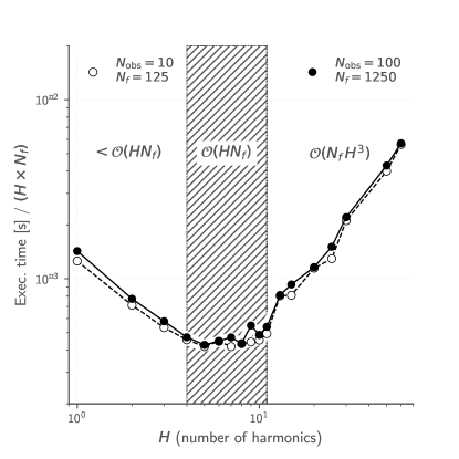
Figure 1.— Computation time of FTP scaled by $NH$ for different numbers of harmonics. For $H\lesssim 3$, FTP scales sublinearly in $H$ (possibly due to a constant overhead per trial frequency, independent of $H$). When $3\lesssim H\lesssim 11$, FTP scales approximately linearly in $H$, and when $H\gtrsim 11$ FTP approaches the $\mathcal{O}(H^{3})$ scaling limit.

For a fixed number of harmonics $H$, the template periodogram scales as $\mathcal{O}(N_{f}\log N_{f})$. However, for a constant number of trial frequencies $N_{f}$, the template algorithm scales as $\mathcal{O}(H^{3})$, and computational resources alone limit $H$ to reasonably small numbers $H\lesssim 15$ (see Figure 1).

3. Implementation

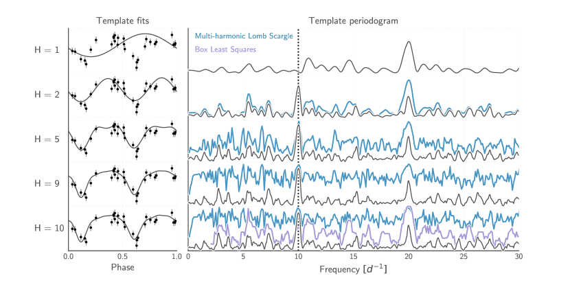
Figure 2.— Template periodograms performed on a simulated eclipsing binary lightcurve (shown phase-folded in the left-hand plots). The top-most plot uses only one harmonic, equivalent to a Lomb-Scargle periodogram. Subsequent plots use an increasing number of harmonics, which produces a narrower and higher peak height around the correct frequency. For comparison, the multi-harmonic extension to Lomb-Scargle is plotted in blue, using the same number of harmonics as the FTP. The Box Least-Squares (Kovács et al., 2002) periodogram is shown in the final plot.

An open-source implementation of the template periodogram in Python is available. Polynomial algebra is performed using the numpy.polynomial module (Jones et al., 2001–). The nfft Python module, which provides a Python implementation of the non-equispaced fast Fourier transform, is used to compute the necessary sums for a particular time series.

No explicit parallelism is used anywhere in the current implementation, however certain linear algebra operations in Scipy use OpenMP via calls to BLAS libraries that have OpenMP enabled.

All timing tests were run on a quad-core 2.6 GHz Intel Core i7 MacBook Pro laptop (mid-2012 model) with 8GB of 1600 MHz DDR3 memory. The Scipy stack (version 0.18.1) was compiled with multi-threaded MKL libraries.

3.1. Comparison with non-linear optimization

In order to evaluate the accuracy and speed of the template periodogram, we have included slower alternative solvers within the Python implementation of the FTP that employ non-linear optimization to find the best fit parameters.

Periodograms computed in Figures 2, 3, and 4 used simulated data. The simulated data has uniformly random observation times, with Gaussian-random, homoskedastic, uncorrelated uncertainties. An eclipsing binary template, generated by fitting a well-sampled, high signal-to-noise eclipsing binary in the HATNet dataset (BD+56 603) with a 10-harmonic truncated Fourier series.

3.1.1 Accuracy

Figure 3.— Comparing accuracy between previous methods that rely on non-linear optimization at each trial frequency with the fast template periodogram described in this paper. Both methods are applied to the same simulated data as shown in Figure 2. The FTP consistently finds more optimal template fits than those found with non-linear optimization, which do not guarantee convergence to a globally optimal solution. The FTP solves for the optimal fit parameters directly, and therefore is able to achieve greater accuracy than template fits done via non-linear optimization.

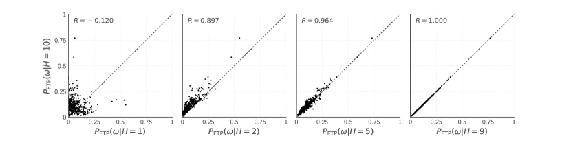
Figure 4.— Comparing the template periodogram calculated with $H=10$ harmonics to the template periodogram using a smaller number of harmonics $H<10$. The template and data used to perform the periodogram calculations are the same as those shown in Figure 2.

For weak signals or signals folded at the incorrect trial period, there may be a large number of local $\chi^{2}$ minima in the parameter space, and thus non-linear optimization algorithms may have trouble finding the global minimum. The FTP, on the other hand, solves for the optimal parameters directly, and thus is able to recover optimal solutions even when the signal is weak or not present.

Figure 3 illustrates the accuracy improvement with FTP. Many solutions found via non-linear optimization are significantly suboptimal compared to the solutions found by the FTP.

Figure 4 compares FTP results obtained using the full template $(H=10)$ with those obtained using smaller numbers of harmonics. The left-most plot compares the $H=1$ case (weighted Lomb-Scargle), which, as also demonstrated in Figure 2, illustrates the advantage of the template periodogram for known, non-sinusoidal signal shapes.

3.1.2 Computation time

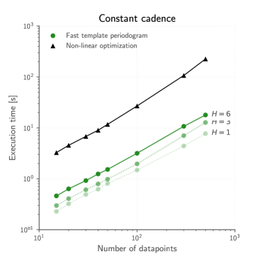
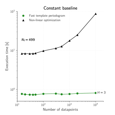
Figure 5.— Computation time of FTP compared with alternative techniques that use non-linear optimization at each trial frequency. Left: timing for the case when $N_{f}=~{}12N_{\rm obs}$, i.e. the cadence of the observations is constant. Right: timing for the case when $N_{f}$ is fixed, i.e. the baseline of the observations are constant. Non-linear optimization techniques scale as $\mathcal{O}(N_{f}N_{\rm obs})$ while the FTP scales as $\mathcal{O}(HN_{f}\log HN_{f}+N_{f}H^{3})$, where $H$ is the number of harmonics needed to approximate the template.

FTP scales asymptotically as $\mathcal{O}(N_{f}H\log N_{f}H)$ with respect to the number of trial frequencies, $N_{f}$ and as $\mathcal{O}(N_{f}H^{3})$ with respect to the number of harmonics in which the template is expanded, $H$. For a given resolving power, however, there is an additional factor of $H$ in each of these terms due to the number of trial frequencies necessary to resolve a periodogram peak being proportional to $H$. However, for reasonable cases ($N_{f}\lesssim 10^{120}$ when $H=5$) the computation time is dominated by computing polynomial coefficients and root finding, both of which scale linearly in $N_{f}$.

The number of trial frequencies needed for finding astrophysical signals in a typical photometric time series is

$$N_{f}=1.75\times 10^{6}\left(\frac{H}{1}\right)\left(\frac{{\rm baseline}}{10~{}{\rm yrs}}\right)\left(\frac{\alpha}{5}\right)\left(\frac{15~{}{\rm mins}}{P_{\rm min}}\right)$$ (89)

where $\alpha$ represents the “oversampling factor,” $\Delta f_{\rm peak}/\Delta f$, where $\Delta f_{\rm peak}\sim 1/{\rm baseline}$ is the typical width of a peak in the periodogram and $\Delta f$ is the frequency spacing of the periodogram.

Extrapolating from the timing of a test case (500 observations, 5 harmonics, 15,000 trial frequencies), the summations account for approximately 5% of the computation time when $N_{f}\sim 10^{6}$. If polynomial computations and root-finding can be improved to the point where they no longer dominate the computation time, this would provide an order of magnitude speedup over the current implementation.

Figure 5 compares the timing of the FTP with that of previous methods that employ non-linear optimization. For the case when $N_{f}\propto N_{\rm obs}$, FTP achieves a factor of 3 speedup for even the smallest test case (15 datapoints), while for larger cases ($N\sim 10^{4}$) FTP offers 2-3 orders of magnitude speed improvement. For the constant baseline case, FTP is a factor of $\sim 2$ faster for the smallest test case and a factor of $\sim 20$ faster for $N_{\rm obs}\sim 10^{4}$. Future improvements to the FTP implementation could further improve speedups by 1-2 orders of magnitude over non-linear optimization.

4. Discussion

Template fitting is a powerful technique for accurately recovering the period and amplitude of objects with a priori known lightcurve shapes. It has been used in the literature by, e.g. Stringer et al. (2019); Sesar et al. (2016, 2010), to analyze RR Lyrae in the SDSS, PS1, and DES datasets, where it has been shown to produce purer samples of RR Lyrae at a given completeness. The computational cost of current template fitting algorithms, however, limits their application to larger datasets or with a larger number of templates.

We have presented a novel template fitting algorithm that extends the Lomb-Scargle periodogram (Lomb, 1976; Scargle, 1982; Barning, 1963; Vaníček, 1971) to handle non-sinusoidal signals that can be expressed in terms of a truncated Fourier series with a reasonably small number of harmonics ($H\lesssim 10$).

The fast template periodogram (FTP) asymptotically scales as $\mathcal{O}(N_{f}H^{2}\log N_{f}H^{2}+N_{f}H^{4})$, while previous template fitting algorithms such as the one used in the gatspy library (VanderPlas, 2016), scale as $\mathcal{O}(N_{f}N_{\rm obs})$. However, the FTP effectively scales as $\mathcal{O}(N_{f}H^{4})$, since the time needed to compute polynomial coefficients and perform zero-finding dominates the computational time for all practical cases ($N_{f}\lesssim 10^{120}$). The $H^{4}$ scaling effectively restricts templates to those that are sufficiently smooth to be explained by a small number of Fourier terms.

FTP also improves the accuracy of previous template fitting algorithms, which rely on non-linear optimization at each trial frequency to minimize the $\chi^{2}$ of the template fit. The FTP routinely finds superior fits over non-linear optimization methods.

An open-source Python implementation of the FTP is available at GitHub. The current implementation could likely be improved by:

1. Improving the speed of the polynomial coefficient calculations and the zero-finding steps. This could potentially yield a speedup of $\sim 1-2$ orders of magnitude over the current implementation.

2. Exploiting the embarassingly parallel nature of the FTP using GPU’s.

For a constant baseline, the current implementation improves existing methods by factors of a $\sim$few for lightcurves with $\mathcal{O}(100)$ observations, and by an order of magnitude or more for objects with more than 1,000 observations. These improvements, taken at face value, are not enough to make template fitting feasible on LSST-sized datasets. However, optimizing the polynomial computations could yield a factor of $\sim 25-100$ speedup over the current implementation, which would make the FTP 1-3 orders of magnitude faster than alternative techniques.

Appendix A Shared-phase multi-band template periodogram

We derive a multi-band extension for the template periodogram for data taken in $K$ filters, with $N_{k}$ observations in the $k$-th filter. We use the same model as the one described in Sesar et al. (2016) in order to illustrate the applicability of the template periodogram to more sophisticated scenarios.

The $i$-th observation in the $k$-th filter is denoted $y^{(k)}_{i}$. We wish to fit a periodic, multi-band template $\mathbf{M}=(\mathbf{M}^{(1)},\mathbf{M}^{(2)},...,\mathbf{M}^{(K)}):[0,2\pi)\rightarrow\mathbb{R}^{K}$ to all observations. We assume the same model used by Sesar et al. (2016), which assumes the relative amplitudes, phase shifts, and offsets are shared across bands:

$$\hat{y}^{(k)}(t|\theta)=\theta_{1}\mathbf{M}^{(k)}(\omega t-\theta_{2})+\theta_{3}+\lambda^{(k)}$$ (A1)

where $\lambda^{(k)}$ is a fixed relative offset for band $k$. The $\chi^{2}$ for this model is

$$\chi^{2}=\sum_{k=1}^{K}\sum_{i=1}^{N_{k}}w^{(k)}_{i}\left(y^{(k)}_{i}-\hat{y}^{(k)}_{i}\right)^{2}$$ (A2)

To make things simpler, we can set the $\lambda^{(k)}$ values to 0 simply by subtracting them off from our observations; this means we take all $y^{(k)}_{i}\rightarrow y^{(k)}_{i}-\lambda^{(k)}$. We have that

$$\chi^{2}=\sum_{k=1}^{K}W^{(k)}\chi^{2}_{k}$$ (A3)

Where $W^{(k)}\equiv\sum_{i=1}^{N_{k}}w^{(k)}_{i}$ and $\sum_{k=1}^{K}W^{(k)}=1$. This means that the system of equations reduces to:

$$0=\frac{\partial\chi^{2}}{\partial\theta_{1}}=\sum_{k=1}^{K}W^{(k)}\left(\widehat{YM}^{(k)}-\theta_{1}\widehat{MM}^{(k)}-\theta_{3}\overline{M}^{(k)}\right)$$ (A4)

for the $\theta_{1}$ parameter, where $\widehat{YM}^{(k)}$, $\widehat{MM}^{(k)}$, $\overline{M}^{(k)}$ are values from the single band case computed for each band individually, holding $W^{(k)}=1$ for each band. That is:

$$\widehat{YM}^{(k)} \equiv\frac{1}{W^{(k)}}\sum_{i=1}^{N_{k}}w^{(k)}_{i}y^{(k)}_{i}\mathbf{M}_{\theta_{2}}^{(k)}(\omega t_{i})$$ (A5)

$$\widehat{MM}^{(k)} \equiv\frac{1}{W^{(k)}}\sum_{i=1}^{N_{k}}w^{(k)}_{i}\left(\mathbf{M}_{\theta_{2}}^{(k)}(\omega t_{i})\right)^{2}$$ (A6)

$$\overline{M}^{(k)} \equiv\frac{1}{W^{(k)}}\sum_{i=1}^{N_{k}}w^{(k)}_{i}\mathbf{M}_{\theta_{2}}^{(k)}(\omega t_{i})$$ (A7)

For the offset $\theta_{3}$, we have

$$0=\frac{\partial\chi^{2}}{\partial\theta_{3}}=\sum_{k=1}^{K}W^{(k)}\left(\bar{y}^{(k)}-\theta_{1}\overline{M}^{(k)}-\theta_{3}\right)$$ (A8)

Where $\bar{y}^{(k)}$ is the weighted-mean for the $k$-th band ($\bar{y}^{(k)}\equiv(1/W^{(k)})\sum_{i=1}^{N_{k}}w^{(k)}_{i}y^{(k)}_{i}$), again with $y^{(k)}_{i}\rightarrow y^{(k)}_{i}-\lambda^{(k)}$.

So if we redefine the quantities $\widehat{YM}$, $\widehat{MM}$, $\overline{M}$, and $\bar{y}$ as weighted averages across the bands, i.e. $\widehat{YM}=\sum_{k=1}^{K}W^{(k)}\widehat{YM}^{(k)}$, etc., the solution for the optimal parameters has the same form:

$$\theta_{1} =\left(\frac{YM}{MM}\right)$$ (A9)

$$\theta_{3} =\bar{y}-\overline{M}\left(\frac{YM}{MM}\right)$$ (A10)

which means that the model for the $k$-th band is

$$\hat{y}^{(k)}=\bar{y}+\left(\frac{YM}{MM}\right)\left(M^{(k)}_{i}-\overline{M}\right)$$ (A11)

The form of the periodogram has the same form as the single-band case:

$$\chi^{2} =\sum_{k=1}^{K}\sum_{i=1}^{N_{k}}w^{(k)}_{i}\left(y^{(k)}_{i}-\hat{y}^{(k)}_{i}\right)^{2}$$ (A12)

$$=\sum_{k=1}^{K}\sum_{i=1}^{N_{k}}w^{(k)}_{i}\left((y^{(k)}_{i}-\bar{y})-\left(\frac{YM}{MM}\right)(M_{i}^{(k)}-\overline{M})\right)^{2}$$ (A13)

$$=\sum_{k=1}^{K}\sum_{i=1}^{N_{k}}w^{(k)}_{i}\left((y^{(k)}_{i}-\bar{y})^{2}-2\left(\frac{YM}{MM}\right)(M_{i}^{(k)}-\overline{M})(y^{(k)}_{i}-\bar{y})+\left(\frac{YM}{MM}\right)^{2}(M_{i}^{(k)}-\overline{M})^{2}\right)^{2}$$ (A14)

$$=YY-2\frac{(YM)^{2}}{MM}+\frac{(YM)^{2}}{MM}$$ (A15)

$$=YY-\frac{(YM)^{2}}{MM}.$$ (A16)

Since there is a single shared offset between the bands (i.e. we assume the mean magnitude is the same in all bands after subtracting $\lambda^{(k)}$), the variance for the signal, $YY$, is not $\sum_{k=1}^{K}\sum_{i=1}^{N_{k}}w^{(k)}_{i}(y^{(k)}_{i}-\bar{y}^{(k)})^{2}$ but $\sum_{k=1}^{K}\sum_{i=1}^{N_{k}}w^{(k)}_{i}(y^{(k)}_{i}-\bar{y})^{2}$.

Construction of the polynomial for the multi-band case can be performed by first computing the polynomial expression for $\psi^{2H}\widehat{MM}=\sum_{k=1}^{K}\sum_{i=1}^{N_{k}}w^{(k)}_{i}\left(\psi^{H}M^{(k)}_{i}\right)^{2}$ and a separate polynomial expression for $\psi^{H}\overline{M}$, which can then be squared and subtracted from $\psi^{2H}\widehat{MM}$ to find $MM^{\prime}=\psi^{2H}MM$.

For $YM^{\prime}=\psi^{H}YM$, we merely compute $\psi^{H}\widehat{YM}^{(k)}$ for each band, take the weighted average of the polynomial coefficients for all bands ($\psi^{H}\widehat{YM}=\sum_{k}^{K}W^{(k)}\psi^{H}\widehat{YM}^{(k)}$) and subtract the $\psi^{H}\bar{y}\overline{M}$ polynomial to get $YM^{\prime}$.

After computing the polynomials $MM^{\prime}$ and $YM^{\prime}$, the polynomial in Equation 80 can be computed quickly and the following steps for finding the optimal model parameters is the same as in the single band case.

The computational complexity of this model scales as $\mathcal{O}(KN_{f}H\log N_{f}H+N_{f}H^{3})$ where $K$ is the number of filters. Since the polynomial zero-finding step is the limiting computation in most real-world applications, the multi-band template periodogram corresponding to the Sesar et al. (2016) model should not be significantly more computationally intensive than the single-band case.

Appendix B Data availibility

The data underlying this article are available in the GitHub repository located at https://github.com/PrincetonUniversity/FastTemplatePeriodogramPaper.

References

- Bakos et al. (2004) Bakos, G., Noyes, R. W., Kovács, G., et al. 2004, PASP, 116, 266
- Baluev (2008) Baluev, R. V. 2008, MNRAS, 385, 1279
- Baluev (2009) —. 2009, MNRAS, 395, 1541
- Baluev (2013a) —. 2013a, MNRAS, 436, 807
- Baluev (2013b) —. 2013b, Astronomy and Computing, 3, 50
- Baluev (2013c) —. 2013c, MNRAS, 431, 1167
- Barning (1963) Barning, F. J. M. 1963, Bull. Astron. Inst. Netherlands, 17, 22
- Bretthorst (2003) Bretthorst, G. L. 2003, Frequency Estimation and Generalized Lomb-Scargle Periodograms (New York, NY: Springer New York), 309–329
- Bretthorst et al. (1988) Bretthorst, G. L., Hung, C.-C., D’Avignon, D. A., & Ackerman, J. J. H. 1988, Journal of Magnetic Resonance, 79, 369
- Chambers et al. (2016) Chambers, K. C., Magnier, E. A., Metcalfe, N., et al. 2016, ArXiv e-prints, arXiv:1612.05560
- Cincotta et al. (1995) Cincotta, P. M., Mendez, M., & Nunez, J. A. 1995, ApJ, 449, 231
- Cooley & Tukey (1965) Cooley, J. W., & Tukey, J. W. 1965, Math. Comput., 19, 297
- Dutt & Rokhlin (1993) Dutt, A., & Rokhlin, V. 1993, SIAM J. Sci. Comput., 14, 1368
- Foreman-Mackey et al. (2017) Foreman-Mackey, D., Agol, E., Ambikasaran, S., & Angus, R. 2017, AJ, 154, 220
- Gaia Collaboration et al. (2016) Gaia Collaboration, Prusti, T., de Bruijne, J. H. J., et al. 2016, A&A, 595, A1
- Graham et al. (2013a) Graham, M. J., Drake, A. J., Djorgovski, S. G., Mahabal, A. A., & Donalek, C. 2013a, MNRAS, 434, 2629
- Graham et al. (2013b) Graham, M. J., Drake, A. J., Djorgovski, S. G., et al. 2013b, MNRAS, 434, 3423
- Hernitschek et al. (2016) Hernitschek, N., Schlafly, E. F., Sesar, B., et al. 2016, ApJ, 817, 73
- Huijse et al. (2012) Huijse, P., Estevez, P. A., Protopapas, P., Zegers, P., & Principe, J. C. 2012, IEEE Transactions on Signal Processing, 60, 5135
- Jones et al. (2001–) Jones, E., Oliphant, T., Peterson, P., et al. 2001–, SciPy: Open source scientific tools for Python, [Online; accessed 2017-01-19]
- Keiner et al. (2009) Keiner, J., Kunis, S., & Potts, D. 2009, ACM Trans. Math. Softw., 36, 19:1
- Kovács et al. (2002) Kovács, G., Zucker, S., & Mazeh, T. 2002, A&A, 391, 369
- Leroy (2012) Leroy, B. 2012, A&A, 545, A50
- Lomb (1976) Lomb, N. R. 1976, Ap&SS, 39, 447
- LSST Science Collaboration et al. (2009) LSST Science Collaboration, Abell, P. A., Allison, J., et al. 2009, ArXiv e-prints, arXiv:0912.0201
- Mortier et al. (2015a) Mortier, A., Faria, J. P., Correia, C. M., Santerne, A., & Santos, N. C. 2015a, A&A, 573, A101
- Mortier et al. (2015b) —. 2015b, BGLS: A Bayesian formalism for the generalised Lomb-Scargle periodogram, ascl:1504.020
- Palmer (2009) Palmer, D. M. 2009, ApJ, 695, 496
- Press & Rybicki (1989) Press, W. H., & Rybicki, G. B. 1989, ApJ, 338, 277
- Rasmussen & Williams (2005) Rasmussen, C. E., & Williams, C. K. I. 2005, Gaussian Processes for Machine Learning (Adaptive Computation and Machine Learning) (The MIT Press)
- Scargle (1982) Scargle, J. D. 1982, ApJ, 263, 835
- Schwarzenberg-Czerny (1996) Schwarzenberg-Czerny, A. 1996, ApJ, 460, L107
- Sesar et al. (2010) Sesar, B., Ivezić, Ž., Grammer, S. H., et al. 2010, ApJ, 708, 717
- Sesar et al. (2016) Sesar, B., Hernitschek, N., Mitrović, S., et al. 2016, ArXiv e-prints, arXiv:1611.08596
- Stringer et al. (2019) Stringer, K. M., Long, J. P., Macri, L. M., et al. 2019, AJ, 158, 16
- VanderPlas (2016) VanderPlas, J. 2016, gatspy: General tools for Astronomical Time Series in Python, Astrophysics Source Code Library, ascl:1610.007
- VanderPlas (2018) VanderPlas, J. T. 2018, ApJS, 236, 16
- VanderPlas & Ivezić (2015) VanderPlas, J. T., & Ivezić, Ž. 2015, ApJ, 812, 18
- Vaníček (1971) Vaníček, P. 1971, Ap&SS, 12, 10
- Zechmeister & Kürster (2009) Zechmeister, M., & Kürster, M. 2009, A&A, 496, 577