Galaxy Clusters from the DESI Legacy Imaging Surveys. I. Cluster Detection

Abstract

Based on the photometric redshift catalog of Zou et al. (2019), we apply a fast clustering algorithm to identify 540,432 galaxy clusters at $z\lesssim 1$ in the DESI legacy imaging surveys, which cover a sky area of about 20,000 deg². Monte-Carlo simulations indicate that the false detection rate of our detecting method is about 3.1%. The total masses of galaxy clusters are derived using a calibrated richness–mass relation that are based on the observations of X-ray emission and Sunyaev & Zel’dovich effect. The median redshift and mass of our detected clusters are about 0.53 and $1.23\times 10^{14}M_{\odot}$, respectively. Comparing with previous clusters identified using the data of the Sloan Digital Sky Survey (SDSS), we can recognize most of them, especially those with high richness. Our catalog will be used for further statistical studies on galaxy clusters and environmental effects on the galaxy evolution, etc.

1 Introduction

Galaxy clusters are the most massive gravitationally bound systems in the universe. They are formed on the cosmic web, tracing the large-scale structure. Galaxy clusters are powerful probes for the structure growth and provide important constraints on cosmological parameters (Kravtsov & Borgani, 2012; Planck Collaboration et al., 2016a). Galaxy clusters are also excellent astrophysical laboratories for studying the galaxy evolution, galaxy collision, gravitational lense, dark matter, and extreme physics in dense environments (Dressler, 1980; Butcher & Oemler, 1984; Moore et al., 1996; Lin & Mohr, 2004; Sand et al., 2004; Kneib & Natarajan, 2011; Kravtsov & Borgani, 2012; Ebeling et al., 2014).

Galaxy clusters are a collection of galaxies that are bonded by the gravity. In addition to stars constituting the luminous matter of galaxies in a cluster, there are multiple observable compositions, including cold gas and dust in galaxies, hot ionized intra-cluster medium (ICM), and dark matter. The multi-component nature of galaxy clusters make them visible across the electromagnetic spectrum. The X-ray emission and Sunyaev & Zel’dovich effect in microwave band originating from the hot ICM (Sunyaev & Zeldovich, 1972; Voit, 2005; Bleem et al., 2015) can be used to detect redshift-independent samples of galaxy clusters (Piffaretti et al., 2011; Reichardt et al., 2013; Planck Collaboration et al., 2016b; Tarrío et al., 2019). These samples usually present relatively high purity and completeness but tend to be high-mass systems. The most effective detections of galaxy clusters are based on large-scale optical and near-infrared imaging data. A variety of cluster finding techniques have been developed attributing to ongoing and upcoming wide and deep large-scale photometric surveys. Generally, there are two kinds of cluster finding methods: one is to find the overdensity of galaxies in the three-dimensional space (Szabo et al., 2011; Wen et al., 2012; Gao et al., 2020) and the other is based on the red-sequence feature (Koester et al., 2007; Hao et al., 2010; Rykoff et al., 2014), which describes the narrow color distribution of red member galaxies in a cluster (also known as the E/S0 redgeline). The red-sequence method utilizes intrinsic color properties of member galaxies, while the overdensity finding method can identify clusters not presenting the red-sequence feature, especially at high redshift.

In Gao et al. (2020), we introduced a new fast clustering algorithm, called as Clustering by Fast Search and Find of Density Peaks (CFSFDP), to identify galaxy clusters from a photometric redshift (photo-z) catalog, which is based on the 7-band photometry of South Galactic Cap U-band Sky Survey (SCUSS; Zhou et al., 2016; Zou et al., 2016), SDSS, and unWISE (Lang et al., 2016) surveys. A total of about 20,000 clusters were discovered over a sky area of 3700 deg² in the south Galactic cap. The latest data release of the DESI (Dark Energy Spectroscopic Instrument; DESI Collaboration et al., 2016) legacy imaging surveys provide 5-band photometry over a sky area of about 20,000 deg² in both northern and southern Galactic caps (Dey et al., 2019). They are composed of three optical components in $grz$ bands and one near-infrared component from the Wide-field Infrared Survey Explorer (WISE) satellite. We have obtained a catalog of accurate photo-zs and stellar masses for more than 0.3 billion morphologically classified galaxies with $r<23$ mag and in the redshift range of $z<1$ (Zou et al., 2019). Based on this catalog, we intend to identify a large sample of galaxy clusters by applying the CFSFDP algorithm. Combining the existing and future spectroscopic data (e.g. SDSS/eBOSS and DESI), we will further statistically investigate the properties of clusters and their member galaxies, environment effect on galaxy evolution, gas inflow and outflow of ICM, and large-scale structures, etc.

This paper is the first of our series work and is organized as follows. Section 2 briefly describes the imaging data and photo-z catalog. Section 3 introduces our detecting method of galaxy clusters. In this section, we apply Monte-Carlo simulations to analyze the false detection rate of our method. The cluster mass and richness are also estimated. Section 4 presents the cross-matching with the Abell and other cluster catalogs based on SDSS data. Section 5 gives a summary. Throughout this paper, we assume a $\Lambda$CDM cosmology with $\Omega_{m}=0.3$, $\Omega_{\Lambda}=0.7$, and $H_{0}=70$ km s^-1 Mpc^-1.

2 Imaging data and photo-z

The DESI is planned to conduct a large-scale spectroscopic survey with 5000-fiber robots installed on the focal plane of the 4m Mayall telescope at Kitt Peak, Arizona (DESI Collaboration et al., 2016). It will measure the redshifts of about 35 million galaxies and quasars over a 5-year period, aiming to explore the structure growth and expansion history of the universe. The DESI legacy imaging surveys are designed to provide spectroscopic targets for DESI. They are compose of three public optical surveys including the Beijing-Arizona Sky Survey (Zou et al., 2017), the Dark Energy Camera Legacy Survey (Blum et al., 2016), and the Mayall $z$-band legacy survey (Silva et al., 2016), which jointly image a sky area of $\sim$14000 deg² in $g$, $r$, and $z$ bands. The legacy surveys also integrate the latest WISE observations and provide deep force photometry in two WISE W1 and W2 bands (Lang et al., 2016; Meisner et al., 2019). The latest data release (DR8) covers an area of about 20,000 deg² in both northern and southern Galactic caps, which includes additional data from Dark Energy Survey (Dark Energy Survey Collaboration et al., 2016). The optical imaging depths are 1.5–2 mag deeper than the SDSS and the infrared $W1$ and $W2$ bands are about 1–1.5 mag deeper than the official WISE data.

The DESI legacy imaging surveys provide deep photometry in 5 bands ranging from optical to near-infrared. Based on the 5-band photometry, we have obtained a catalog of accurate photometric redshifts and stellar masses for galaxies classified by the legacy surveys (see more details in Zou et al., 2019). The catalog is updated to the DESI DR8 release, which contains about 0.3 billion galaxies with $r<23$ mag. The redshift and mass ranges are about $z<1$ and $8.4<\log(M_{*})<11.9$, respectively. The redshift bias is ignorable and the corresponding accuracy is about 0.017. The stellar mass shows internal and external dispersions of about 0.09 and 0.22 dex, respectively. We have applied some quality cuts to get clean photometry when constructing the photo-z catalog. In order to select galaxies with more reliable photo-z estimations, we limit our galaxy samples to meet the following conditions:

$$\begin{split}\mathrm{MAG\_ABS\_R}<-20.5,\\ \mathrm{PHOTO\_ZERR}<0.1,\end{split}$$ (1)

where MAG_ABS_R is the $r$-band absolute magnitude and PHOTO_ZERR is the photo-z error. The cut of the photo-z error is used to eliminate galaxies with large photo-z uncertainty. The cut of the absolute magnitude is set to keep more luminous galaxies and hence improve the completeness. Finally, a total of 0.18 billion galaxies are left for identifying clusters in the rest of this paper.

3 Cluster Identification

3.1 Detecting method

The CFSFDP approach was first proposed by Rodriguez & Laio (2014) and has been widely used for cluster analyses in a wide range of fields. In this approach, the cluster center is the point that having a higher density than their neighbors and meanwhile it is adequately far away from other points having higher densities. It was demonstrated that this approach can intuitively detect clusters and their members and automatically exclude the outliers. The CFSFDP is characterized in the algorithm simplicity and efficiency so that it is very suitable for identifying galaxy clusters in astronomical photometric surveys. We have successfully applied this approach to find clusters in the south Galactic cap with photo-zs based on the multi-wavelength data from SCUSS, SDSS, and unWISE (Gao et al., 2020). The photometric redshifts are used to project the galaxies onto the 2D sky plane and then the CFSFDP is used to identify the overdensity peaks. We adopt a similar method as used in Gao et al. (2020). The details of the cluster detecting process are described as below.

1. Galaxies in our photo-z catalog are divided into small equal-area sky patches (or pixels) in the Hierarchical Equal Area and isoLatitude Pixelisation (HEALPix) projection. We adopt the resolution parameter of $\mathrm{nside}=64$, giving each HEALPix pixel area of about 0.89 deg². The above pixelation is to facilitate the parallelization of cluster detecting.

2. For each galaxy at a given redshift $z$ in a specified HEALPix pixel, we calculate the local density ($\Phi$) and background density ($\Phi_{\mathrm{bkg}}$). These two quantities are computed from the galaxies in this pixel and its surrounding 8 neighbor pixels, which have a total area of about 8 deg². The area is large enough to estimate a proper local background. $\Phi$ is computed as the number of galaxies with distance $R<0.5$ Mpc in a redshift slice of $z\pm 0.04(1+z)$. $\Phi_{\mathrm{bkg}}$ is computed as the number of galaxies with $R>1$ Mpc (to avoid the possible cluster region) in the same redshift slice. The background density is scaled to the same area as used in the calculation of the local density. Another crucial parameter $D$ in Mpc is defined as the shortest distance of the specified galaxy to other galaxies with higher $\Phi$.

3. The cluster centers should be located on the overdensity peaks with large enough local density and adequately far away from other peaks. They are identified as the galaxies with $\Phi>4\Phi_{\mathrm{bkg}}$ and $D>1$ (typical cluster radius is less than 1 Mpc). If there are multiple galaxies with the same local density, we assign the brightest galaxy in $r$ band as the cluster center. This cluster center is not always the brightest cluster galaxy (BCG) that is usually close to the densest region. We simply regard the $r$-band brightest galaxy within 0.5 Mpc around the density peak as the BCG. Since each galaxy is pointed to the nearest neighbor with higher $\Phi$, the galaxies in the redshift slice can be traced and clustered to the cluster center. The clustered galaxies are roughly considered as the member candidates. With these members, we can calculate the average position and redshift for each cluster.

4. The number of member galaxies within 1 Mpc around the cluster center are calculated, which is subtracted the local background and denoted as $N_{\mathrm{1Mpc}}$. $N_{\mathrm{1Mpc}}$ is regarded as the first-order approximate of the cluster richness. We require that clusters should have $N_{\mathrm{1Mpc}}>10$. The total $r$-band luminosity of member galaxies around the cluster center ($L_{\mathrm{1Mpc}}$) is calculated in unit of $L^{*}$, where $L^{*}$ is the characteristic luminosity. $L_{\mathrm{1Mpc}}$ will be used as a proxy of the cluster mass and richness later. When calculating $L_{\mathrm{1Mpc}}$, we also subtract the background luminosity that is estimated in the same way as $\Phi_{\mathrm{bkg}}$. Note that the richness and luminosity in this paper are not corrected for the variation of the imaging depth. Such corrections are quite complicated due to the mixture nature of our data from three different optical surveys plus the WISE infrared survey and the selection of the photo-z sample. Actually, more than 90% of the area has the $5\sigma$ $r$-band magnitude limit larger than 23.4 mag. As presented in Zou et al. (2019), the completeness of galaxies at $r<23$, which is the magnitude cut for the photo-z catalog used in this paper, is higher than 90%. As a preliminary estimate, the correction of the richness or luminosity would be less than 10%.

The above process is performed over the photo-z catalog. Finally, we obtain a catalog of 540,432 galaxy clusters at $z\lesssim 1$. The catalog content is described in Appendix A. Figure 1 presents four examples of our detected clusters at different redshifts. As can be seen from this figure, the prominent overdensity features of galaxies make them easily identified from our imaging data by using the above cluster finding method.

Figure 1: Four examples of galaxy clusters at different redshifts: (a) $z=0.05$, (b) $z=0.34$, (c) $z=0.54$, and (d) $z=0.82$. The small green circle shows the galaxy at the local density peak and the cyan circle at the center marks the BCG. If these two galaxies are the same, the cyan circle will cover the green one. The magenta plus shows the average position of member galaxies. The big yellow dashed circle indicates a radius of 0.5 Mpc. In each panel, we also display the information about the galaxy at the density peak (Peak), the BCG, and average of the members (Mean), including the position (RA, DEC), photo-z (Photo-z), and spectroscopic redshift (Spec-z; if not existing, just giving $-10$). The cluster properties are also presented, including $N_{\mathrm{1Mpc}}$ (N_1MPC), richness (RICHNESS), total mass (M_500), and characteristic radius (R_500) (see Section 3.3 and Table 2). North is up and east is left.

3.2 Reliability analysis

The cluster detecting process is executed in relatively large redshift slices due to the photo-z uncertainty. It is inevitable to introduce the project effect and hence cause false cluster detections. In addition, the local background fluctuation will also bring contaminations to the low-richness clusters. We perform a Monte-Carlo simulation to evaluate the detecting approach and estimate the false detection rate following a similar method of Wen & Han (2011). The simulation is based on the actual photometric data and the specific steps are described as follows. (1) An arbitrary region with an area of 400 deg² is selected in our photo-z catalog. (2) Galaxies in this region are redistributed on the sky with random walks from original locations in the range of 1–2.5 Mpc and then their redshifts are shuffled. This step can generate new random galaxy backgrounds and meanwhile retain the project effect in some degree. (3) The same clustering detecting process used in this paper is applied to these mock galaxies and to finding fictitious clusters.

We make a total of 10 simulations and identify the false detections in these simulations. The false rate is defined as the ratio of the number of false clusters identified in the simulation to the number of detected clusters in the original catalog. Figure 2 presents the average false rate of the above 10 simulations as functions of redshift and $N_{\mathrm{1Mpc}}$. From this figure, we can see that the false rate generally increases with redshift and decreases with $N_{\mathrm{1Mpc}}$. In other words, the contamination of our detections is more serious for distant or low-richness clusters. The overall false rate is about 3.1% and it can go up to about 7-8% at high redshift and lowest richness.

It should be noticed that the above simulations can estimate the false detections inducing by chance associations and part of false detections caused by the projection effect of uncorrelated structures, because we generate random galaxy backgrounds with limited position changes. Nevertheless, the projection effects include the impacts from both correlated and uncorrelated large-scale structures. It is very important to estimate their effect on basic cluster properties (e.g. richness and halo mass) especially when the cluster catalog is used to constrain the cosmological parameters. For example, Costanzi et al. (2019) combined both real data and numerical simulations to characterize the impact of projection effects on the redMaPPer cluster catalog and they found that the projection effect obviously biases the cosmological parameter measurements. Principally, we can use the mock catalogs from $N$-body simulations to assess the reliability of our cluster finder. However, the synthetic data are model-dependent and are probably biased from realistic observations, such as the halo occupation distribution of cluster galaxies, galaxy color distributions, photometric uncertainty and corresponding photo-z uncertainty. Considering the complexity of the projection effects, we expect an investigation of their impact on the reliability of our detecting method and on the following mass estimation in future work.

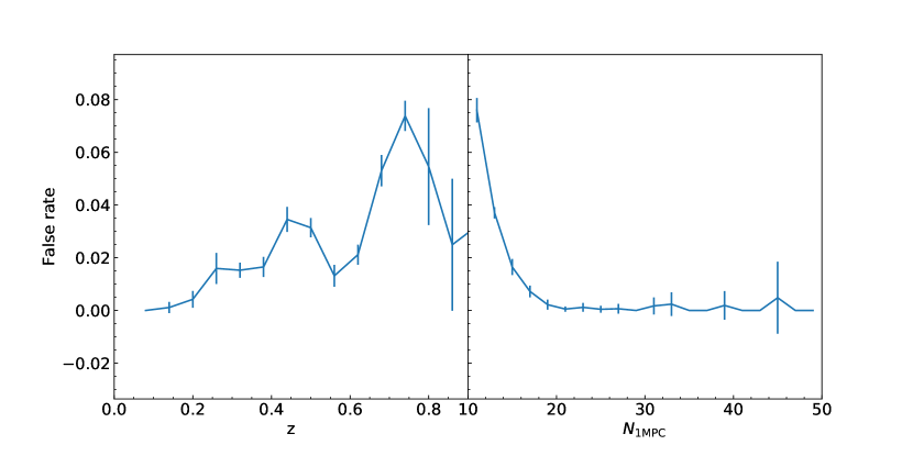
Figure 2: Left: false detection rate as function of redshift. Right: false detection rate as function of $N_{\mathrm{1Mpc}}$. The error bar shows the standard deviation of 10 simulations.

3.3 Mass and richness estimation

The X-ray and SZ surveys provide large samples of galaxy clusters at different redshifts, which has reasonably estimates of the cluster mass with relatively small intrinsic scatter. The observables, such as luminosity and temperature in X ray and the integrated Comptonisation parameter (or SZ parameter), are tightly linking to the cluster mass via scaling relations.

Wen & Han (2015) collected a sample of 1,192 clusters from the literature and scaled the cluster masses derived by different authors to a unified calibration. These samples are limited to match the galaxy clusters identified from SDSS with the maximum redshift is 0.75. The clusters at high redshift are insufficient, so we supplement the sample of Wen & Han (2015) with other clusters from X-ray and SZ observations (Piffaretti et al., 2011; Takey et al., 2013, 2014; Wen & Han, 2015; Takey et al., 2016; Planck Collaboration et al., 2016b). The cluster masses in different catalogs were estimated using different mass proxies and scaling relations, so it is necessary to recalibrate the masses. So we use the rescaling relations derived by Wen & Han (2015) to calibrate the cluster mass for these additional data. All the cluster masses are rescaled to the standard of Vikhlinin et al. (2009). We should note that the published Planck catalog has not applied the Eddington bias correction, which can systematically bias the SZ masses (Battaglia et al., 2016; Medezinski et al., 2018). The above recalibration process can reduce this kind of systematic effects. Here, the cluster mass is denoted as $M_{500}$, which is the mass within a characteristic radius ($R_{500}$). $R_{500}$ is defined as the radius within which the mean density of a cluster is 500 times the critical density of the universe ($\rho_{c}$). According to the definition, $M_{500}$ and $R_{500}$ satisfy the following relation:

$$M_{500}=\frac{4\pi}{3}R_{500}^{3}\times 500\rho_{c}.$$ (2)

We collect 3,157 clusters with reliable estimations of $M_{500}$ and $R_{500}$, which spreads over the whole celestial sphere. They are listed in a separate table of Table 3 in Appendix B, which we called as the calibration catalog.

As described in Gao et al. (2020), $L_{\mathrm{1Mpc}}$ is used as an optical proxy of the cluster mass. We also use $L_{\mathrm{1Mpc}}$ to estimate the total mass of our clusters. The galaxy clusters detected in this work are cross-matched with the clusters in the calibration catalog of Table 3, following a similar procedure in Bleem et al. (2020): 1) ranking the clusters in the calibration catalog by the decreasing mass (equivalent to the richness); 2) matching each cluster in the calibration catalog to the richest cluster in our catalog with a redshift error of $\Delta z=0.06(1+z)$ and a projected separation error of 1 Mpc; 3) removing each matched cluster from our catalog and repeating the above matching process for all clusters in the calibration catalog. As a result, we find 1,797 matched clusters that can be used to determine the relation between $L_{\mathrm{1Mpc}}$ and $M_{500}$. The left panel of Figure 3 shows $M_{500}$ as function of $L_{\mathrm{1Mpc}}$. We can see that there is a tight correlation between these two quantities. The correlation can be described by the following equation:

$$\begin{split}\log(M_{500})&=a\log(L_{\mathrm{1Mpc}})+b\log(1+z)+c,\\ \mathrm{or~{}}M_{500}&=10^{c}L_{\mathrm{1Mpc}}^{a}(1+z)^{b},\end{split}$$ (3)

where $a$, $b$, and $c$ are constants to be determined and the term of $(1+z)$ is regarded as the correction term for the redshift evolution and incompleteness.

The above luminosity–mass relation suffers from the Malmquist bias as the cluster sample is constructed with flux-limited X-ray and SZ observations. The Malmquist bias makes the sample preferentially contain brighter or massive clusters. It is especially serious for clusters with low richness at high redshift. The compilations of our clusters are from X-ray and SZ observations with different depths, which may mitigate the effect of the Malmquist bias, but also induces the complication of the bias correction. We hope a further investigation of this problem in the future. Considering the bias, we assign the data with weight of $\frac{L_{\mathrm{1Mpc}}}{z}$ when fitting the data with Equation (3). This will put more weight to the clusters with larger richness and at lower redshift. We get the best-fit parameters via weighted linear regression: $a=0.81\pm 0.02$, $b=0.50\pm 0.14$, and $c=12.61\pm 0.04$. The middle and right panels of Figure 3 presents the residual between observed $M_{500}$ and the fitted one as functions of $L_{500}$ and redshift. The overall RMS of the residual is about 0.2 dex. The residual RMS changes with $L_{\mathrm{1Mpc}}$, ranging from 0.28 to 0.12 dex. The residual biases at high redshift, partly reflecting the Malmquist bias. We apply the Equation (3) to estimate $M_{500}$ and Equation (2) to estimate $R_{500}$ for our detected clusters. We also use the Equation (17) in Wen & Han (2015) to estimate the richness. These parameters are included in Table 2.

Figure 3: Left: correlation between $\log(M_{500}$) and $\log(L_{\mathrm{1Mpc}})$. The error bar shows the error of $\log(M_{500}$). Middle: the difference ($\Delta\log(M_{500})$) between $\log(M_{500})$ and fitted values as function of $L_{\mathrm{1Mpc}}$. The red error bar shows the median and standard deviation in each luminosity bin. Right: $\Delta\log(M_{500})$ as function of redshift. The red error bar shows the median and standard deviation in each redshift bin. The horizontal line displays $\Delta\log(M_{500})=0$.

3.4 Cluster statistics and photo-z accuracy

Figure 9 shows the parameter distributions for the whole 540,432 galaxy clusters detected in this paper. The median redshift is about 0.53 and the number density decreases at $z>\sim 0.6$, where the cluster detection should be more incomplete. The median richness is about 22.5. The range of the total mass $\log(M_{500})$ is 13.5–14.8 and the median is about 14.1 (equivalent to $1.23\times 10^{14}M_{\odot}$). The characteristic radius of $R_{500}$ ranges from about 0.4 Mpc to 1.0 Mpc and the median value is about 0.63 Mpc.

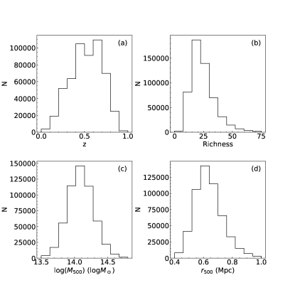
Figure 4: Distributions of redshift (a), richness (b), $\log(M_{500})$ (c), and $R_{500}$ (d) for our clusters.

Figure 5 displays both the distributions of $r$-band depth and number density of our clusters over the DESI imaging footprint. Note that the depth is referred to $5\sigma$ $r$-band magnitude limit for extended sources with the correction of the Galactic extinction. The depth map in Figure 5a shows three distinct regions with different imaging depths, which reflects that the observing data were obtained by different facilities. The general depth differences among these three components are about 0.6 mag. Although the depth is inhomogeneous across the survey footprint, we still obtain uniformly distributed cluster samples attributing to our relatively conservative magnitude cut of our photo-z catalog (see Figure 5b). In order to more clearly show the effect of the imaging depth on our cluster detection, we present the number densities as function of redshift for three subsamples of our clusters under different $r$-band depths in Figure 6. From this figure, we can see that the imaging depth only affects the cluster detection at $z>0.4$. More clusters are detected in the deeper area and it becomes more pronounced as the redshift increases.

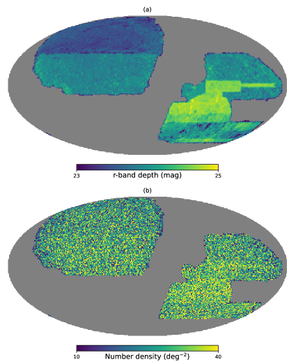
Figure 5: (a) The $r$-band depth map in Mollview projection. (b) Number density distribution of our detected clusters.

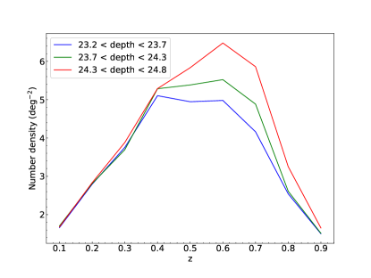
Figure 6: Number density as function of redshift for three subsamples of our clusters under different $r$-band imaging depths. The redshift bin is 0.1.

The photo-z accuracy of our galaxy clusters are estimated by comparing the photometric redshifts of the BCGs in our catalog with spectroscopic redshifts collected by Zou et al. (2019). There are a total of 12,2390 BCGs with spectroscopic redshifts. The top panel of Figure 7 shows the comparison between the photometric redshift ($z_{\mathrm{phot}}$) and spectroscopic redshift ($z_{\mathrm{spec}}$). The bottom panel presents the photo-z accuracy of $\Delta z_{\mathrm{norm}}=(z_{\mathrm{phot}}-z_{\mathrm{spec}})/(1+z_{\mathrm{spec}})$ as function of $z_{\mathrm{spec}}$. We can see that the photo-z accuracy changes from about 0.01 at $z\sim 0.1$ to about 0.024 at $z\sim 0.9$. The redshift histogram in Figure 8 shows the distribution of $\sigma_{\Delta z_{\mathrm{norm}}}$ of the total sample. The overall photo-z accuracy is $\sigma_{\Delta z_{\mathrm{norm}}}=0.012$. In addition, most of the galaxy clusters used for mass calibration as described in Section 3.3 have reliable redshifts. We also estimate our cluster photo-z accuracy using these confirmed clusters, which is shown in the blue histogram of Figure 8. Such a comparison also gives a similar photo-z accuracy of $\sigma_{\Delta z_{\mathrm{norm}}}=0.013$.

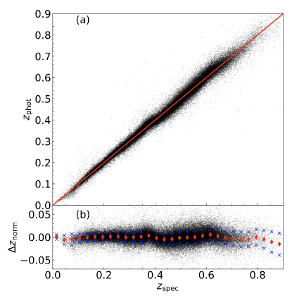
Figure 7: (a) Comparison between photometric and spectroscopic redshifts of the BCGs in our cluster catalog. The diagonal line denotes $z_{\mathrm{phot}}=z_{\mathrm{spec}}$. (b) $\sigma_{\Delta z_{\mathrm{norm}}}$ as function of $z_{\mathrm{spec}}$. The red diamonds and blue crosses display the medians and standard deviations in different redshift bins.

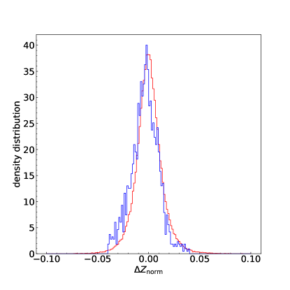
Figure 8: The $\sigma_{\Delta z_{\mathrm{norm}}}$ distribution (red) of the BCGs in our clusters, which have spectroscopic redshift measurements. The blue histogram is the $\sigma_{\Delta z_{\mathrm{norm}}}$ for confirmed galaxy clusters with reliable redshift measurements, which are detected in X-ray and SZ-effect observations.

4 Matching with other cluster catalogs

The most famous cluster catalog is the Abell catalog, which was constructed by the visual identification on the photographic plates. There are also several catalogs of galaxy clusters identified from the SDSS photometric data. These catalogs are either based on the red-sequence feature or the overdensity feature in the photo-z space. Through matching our catalog with these catalogs, we can check the detecting repeatability of the clusters from both shallower photometric data and deeper DESI imaging data. Such comparisons can also indicate the reliability of our cluster detection. The Abell clusters were visually identified as galaxy overdensities (Abell et al., 1989). Among other catalogs that are based on SDSS data, the clusters of MaxBCG (Koester et al., 2007), GMBCG (Hao et al., 2010), and redMaPPer (Rykoff et al., 2014) were identified through the red-sequence feature, while the clusters of AMF (Szabo et al., 2011) and WHL15 (Wen & Han, 2015) were obtained using the overdensity feature. We summarize the redshift range, adopted method and number of clusters in the DESI footprint of these catalogs in Table 1. If the clusters in the Abell catalog have spectroscopic redshifts, we use their spectroscopic redshifts as the distance indicator. For those clusters without redshifts in the Abell catalog, we only use our photo-z as the distance tracer to match the clusters. The projected separation is limited to 1 Mpc, which is set to be a little larger than the characteristic radius ($R_{500}$ of most clusters as shown in Figure 9). For the SDSS cluster catalogs, we match them with our cluster catalog using a redshift tolerance of $\Delta z<0.06(1+z)$ and the same separation tolerance. The larger the separation tolerance is set, the more real clusters would be matched in consideration of the uncertainty of the cluster center, while more possible false association would occur and vice versa. The matching results with our catalog are listed in Table 1.

Table 1: Matching our catalog with other cluster catalogs

Catalog	Redshift	Method	Number	Matched	Percent
(1)	(2)	(3)	(4)	(5)	(6)
Abell	$\cdots$	visual overdensity	2,298	2,143	93.3%
MaxBCG	$0.1<z<0.3$	red sequence	13,806	10,494	76.0%
GMBCG	$0.1<z<0.55$	red sequence	55,317	29,980	54.2%
AMF	$0.045<z<0.78$	overdensity	44,692	33,731	75.5%
redMaPPer	$0.08<z<0.55$	red sequence	25,835	24,645,	95.4%
WHL15	$0.05<z<0.8$	overdensity	121,480	80,686	66.4%

As checked, most of the mismatching clusters in those catalogs based on the SDSS data are the clusters with lower richness or at higher redshift, which are possible false detections. We select two representative catalogs, redMaPPer and WHL15, to show the matching rates as function of redshift and richness and present the comparison of richness and redshift with those in our catalog in Figure 9. Generally, the matching rate increases as the richness increases or the redshift decreases. The richnesses among these catalogs show good correlations, although there are somewhat large scatters. The photo-z also shows pretty correlations. Compared to the WHL15 photo-z, the photo-z of the redMaPPer clusters is more consistent with that of our clusters.

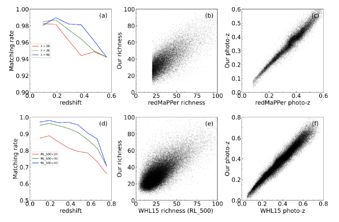
Figure 9: (a) The matching rate between the redMaPPer catalog and our catalog as function of redshift and richness. (b) The correlation between the richness of our clusters and that of the redMaPPer clusters ($\lambda)$. (c) The correlation between the photo-z of our clusters and that of the redMaPPer clusters. (d) The matching rate between the WHL15 catalog and our catalog as function of redshift and richness. (e) The correlation between the richness of our clusters and that of the WHL15 clusters (RL_500). (f) The correlation between the photo-z of our clusters and that of the WHL15 clusters.

5 Summary

Galaxy clusters are excellent probes for studying galaxy formation and evolution in the dense environments and they can be also used to constrain cosmological parameters. Using the photometric redshift catalog of Zou et al. (2019), we identify a catalog of galaxy clusters over the 20000-deg² sky footprint of the DESI legacy imaging surveys. This sample of clusters will be used to statistically study the galaxy clusters at $z<1$, the galaxy environment, ICM, large-scale structures of the universe, etc. As the first of a series work, this paper is focused on the cluster detection.

In total, we identify 540,432 galaxy clusters with $z\lesssim 1$. These clusters are uniformly distributed over the imaging footprint. Monte-Carlo simulations show that the false detection rate is about 3.1% and it becomes worse as the redshift increases or the richness decreases. The false rate at high redshift or low richness can reach up to about 8%. We utilize the mass measurements from X-ray and radio observations to calibrate the total mass and richness of the detected clusters by using the optical luminosity $L_{\mathrm{1Mpc}}$. The median mass and richness are about $1.23\times 10^{14}M_{\odot}$ and 22.5, respectively. Comparing our catalog with the Abell catalog, we can recover almost all Abell clusters. We also compare our detected clusters with those based on the SDSS data that are about 2 magnitude shallower than the DESI imaging surveys. It is found that we can recognize most of the clusters identified from SDSS, especially those with high richness.

Appendix A Information about our cluster catalog

In total, we obtain 540,432 galaxy cluster with a false detection rate of about 3.1%. Table 2 lists the content contained in our catalog. It includes the position and redshift of the cluster center, which is the galaxy at the local density peak. The catalog also includes the basic information of the BCG including the position, redshift, observed magnitudes, absolute magnitudes, and stellar mass, which are inherited from the photo-z catalog. The cluster properties estimated in this paper are also contained in this catalog. This catalog will be uploaded to CDS and it is also available at http://batc.bao.ac.cn/~zouhu/doku.php?id=projects:desi_clusters:start.

Table 2: Column description for our cluster catalog

Column	Unit	Format	Description
CLUSTER_ID		Long	Cluster ID
RA_PEAK	degree	Double	R.A. for the density peak (J2000)
DEC_PEAK	degree	Double	decl. for the density peak (J2000)
PZ_PEAK		Float	Photometric redshift for the density peak
SZ_PEAK		Float	Spectroscopic redshift for the density peak if existing
DEN_PEAK		Integer	Local density $\Phi$ for the density peak
BKG_PEAK		Float	Local background density $\Phi_{\mathrm{bkg}}$ for the density peak
RA_MEAN	degree	Double	Mean R. A. of possible members
DEC_MEAN	degree	Double	Mean decl. of possible members
N_1MPC		Integer	Number of member galaxies within 1 Mpc from the cluster center
L_1MPC	$L^{*}$	Float	Total luminosity of member galaxies within 1 Mpc from the cluster center
M_500	$\log_{10}(M_{\odot})$	Float	Total mass of the cluster $M_{500}$
R_500	Mpc	Float	Characteristic radius $R_{500}$
RICHNESS		Float	Cluster richness
RA_BCG	degree	Double	R.A. for the BCG (J2000)
DEC_BCG	degree	Double	decl. for the BCG (J2000)
PZ_BCG		Float	Photometric redshift for the BCG
PZERR_BCG		Float	Photometric redshift error for the BCG
SZ_BCG		Float	Spectroscopic redshift for the BCG if existing
MAG_G_BCG	mag	Float	$g$-band magnitude for the BCG
MAG_R_BCG	mag	Float	$r$-band magnitude for the BCG
MAG_Z_BCG	mag	Float	$z$-band magnitude for the BCG
MAG_W1_BCG	mag	Float	$W1$-band magnitude for the BCG
MAG_W2_BCG	mag	Float	$W2$-band magnitude for the BCG
MAGERR_G_BCG	mag	Float	$g$-band magnitude error for the BCG
MAGERR_R_BCG	mag	Float	$r$-band magnitude error for the BCG
MAGERR_Z_BCG	mag	Float	$z$-band magnitude error for the BCG
MAGERR_W1_BCG	mag	Float	$W1$-band magnitude error for the BCG
MAGERR_W2_BCG	mag	Float	$W2$-band magnitude error for the BCG
MAG_ABS_G_BCG	mag	Float	$g$-band absolute magnitude for the BCG
MAG_ABS_R_BCG	mag	Float	$r$-band absolute magnitude for the BCG
MAG_ABS_Z_BCG	mag	Float	$z$-band absolute magnitude for the BCG
MAG_ABS_W1_BCG	mag	Float	$W1$-band absolute magnitude for the BCG
MAG_ABS_W2_BCG	mag	Float	$W2$-band absolute magnitude for the BCG
MASS_BEST_BCG	$\log_{10}(M_{\odot})$	Float	Logarithmic stellar mass for the BCG
MASS_INF_BCG	$\log_{10}(M_{\odot})$	Float	Lower limit of logarithmic stellar mass with 68% confidence level for the BCG
MASS_SUP_BCG	$\log_{10}(M_{\odot})$	Float	Upper limit of logarithmic stellar mass with 68% confidence level for the BCG

Appendix B Galaxy clusters with the total mass measurements from X-ray and radio observations

Table 3 lists the galaxy clusters detected by X-ray and SZ-effect observations and their total masses are effectively estimated and rescaled by us to a unified calibration. The characteristic radius of $R_{500}$ is calculated according to Equation (2).

Table 3: Galaxy clusters with the total mass measurements from X-ray and SZ-effect observations

ID	RA	DEC	Z	M500	E_M500	R500	E_R500	REF
(1)	(2)	(3)	(4)	(5)	(6)	(7)	(8)	(9)
1	4.57107	16.29432	0.55	4.11	0.77	0.93	0.06	W15
2	8.32687	-21.41319	0.19	0.99	0.20	0.66	0.04	T13
3	9.82501	0.69981	0.28	0.66	0.13	0.56	0.04	W15
4	9.84351	0.80273	0.41	1.62	0.31	0.72	0.05	T13, T16
5	9.92591	0.75922	0.42	1.27	0.25	0.66	0.04	T13, T16
6	10.16344	25.51840	0.15	1.24	0.24	0.72	0.05	T13
7	10.48690	25.53105	0.13	0.93	0.19	0.66	0.04	T13
8	10.62969	0.85368	0.16	0.69	0.15	0.59	0.04	T13, T16
9	10.71922	0.71671	0.27	1.16	0.23	0.68	0.04	T13, T16
10	10.72397	-9.57311	0.41	1.49	0.29	0.70	0.05	T13

References

- Abell et al. (1989) Abell, G. O., Corwin, H. G., Jr., & Olowin, R. P. 1989, ApJS, 70, 1
- Banerjee et al. (2018) Banerjee, P., Szabo, T., Pierpaoli, E., et al. 2018, New A, 58, 61
- Battaglia et al. (2016) Battaglia, N., Leauthaud, A., Miyatake, H., et al. 2016, J. Cosmology Astropart. Phys, 2016, 013. doi:10.1088/1475-7516/2016/08/013
- Bleem et al. (2015) Bleem, L. E., Stalder, B., de Haan, T., et al. 2015, ApJS, 216, 27
- Bleem et al. (2020) Bleem, L. E., Bocquet, S., Stalder, B., et al. 2020, ApJS, 247, 25. doi:10.3847/1538-4365/ab6993
- Blum et al. (2016) Blum, R. D., Burleigh, K., Dey, A., et al. 2016, American Astronomical Society Meeting Abstracts #228 228, 317.01
- Butcher & Oemler (1984) Butcher, H. & Oemler, A. 1984, ApJ, 285, 426
- Cole et al. (2000) Cole, S., Lacey, C. G., Baugh, C. M., et al. 2000, MNRAS, 319, 168
- Costanzi et al. (2019) Costanzi, M., Rozo, E., Rykoff, E. S., et al. 2019, MNRAS, 482, 490
- Dark Energy Survey Collaboration et al. (2016) Dark Energy Survey Collaboration, Abbott, T., Abdalla, F. B., et al. 2016, MNRAS, 460, 1270
- DESI Collaboration et al. (2016) DESI Collaboration, Aghamousa, A., Aguilar, J., et al. 2016, arXiv e-prints, arXiv:1611.00036
- Dey et al. (2019) Dey, A., Schlegel, D. J., Lang, D., et al. 2019, AJ, 157, 168
- Dressler (1980) Dressler, A. 1980, ApJ, 236, 351
- Ebeling et al. (2014) Ebeling, H., Stephenson, L. N., & Edge, A. C. 2014, ApJ, 781, L40
- Gao et al. (2020) Gao, J., Zou, H., Zhou, X., et al. 2020, PASP, 132, 024101
- Hao et al. (2010) Hao, J., McKay, T. A., Koester, B. P., et al. 2010, ApJS, 191, 254
- Kneib & Natarajan (2011) Kneib, J.-P. & Natarajan, P. 2011, A&A Rev., 19, 47
- Koester et al. (2007) Koester, B. P., McKay, T. A., Annis, J., et al. 2007, ApJ, 660, 239
- Kravtsov & Borgani (2012) Kravtsov, A. V. & Borgani, S. 2012, ARA&A, 50, 353
- Lang et al. (2016) Lang, D., Hogg, D. W., & Schlegel, D. J. 2016, AJ, 151, 36
- Lin & Mohr (2004) Lin, Y.-T. & Mohr, J. J. 2004, ApJ, 617, 879
- Medezinski et al. (2018) Medezinski, E., Battaglia, N., Umetsu, K., et al. 2018, PASJ, 70, S28. doi:10.1093/pasj/psx128
- Meisner et al. (2019) Meisner, A. M., Lang, D., Schlafly, E. F., et al. 2019, PASP, 131, 124504
- Moore et al. (1996) Moore, B., Katz, N., Lake, G., et al. 1996, Nature, 379, 613
- Piffaretti et al. (2011) Piffaretti, R., Arnaud, M., Pratt, G. W., et al. 2011, A&A, 534, A109
- Planck Collaboration et al. (2016a) Planck Collaboration, Ade, P. A. R., Aghanim, N., et al. 2016a, A&A, 594, A13
- Planck Collaboration et al. (2016b) Planck Collaboration, Ade, P. A. R., Aghanim, N., et al. 2016b, A&A, 594, A27
- Reichardt et al. (2013) Reichardt, C. L., Stalder, B., Bleem, L. E., et al. 2013, ApJ, 763, 127
- Rodriguez & Laio (2014) Rodriguez, A., & Laio, A. 2014, Science, 344, 1492
- Rykoff et al. (2014) Rykoff, E. S., Rozo, E., Busha, M. T., et al. 2014, ApJ, 785, 104
- Sand et al. (2004) Sand, D. J., Treu, T., Smith, G. P., et al. 2004, ApJ, 604, 88
- Silva et al. (2016) Silva, D. R., Blum, R. D., Allen, L., et al. 2016, American Astronomical Society Meeting Abstracts #228 228, 317.02
- Sunyaev & Zeldovich (1972) Sunyaev, R. A., & Zeldovich, Y. B. 1972, Comments on Astrophysics and Space Physics, 4, 173
- Szabo et al. (2011) Szabo, T., Pierpaoli, E., Dong, F., Pipino, A., & Gunn, J. 2011, ApJ, 736, 21
- Takey et al. (2011) Takey, A., Schwope, A., & Lamer, G. 2011, A&A, 534, A120
- Takey et al. (2013) Takey, A., Schwope, A., & Lamer, G. 2013, A&A, 558, A75
- Takey et al. (2014) Takey, A., Schwope, A., & Lamer, G. 2014, A&A, 564, A54
- Takey et al. (2016) Takey, A., Durret, F., Mahmoud, E., et al. 2016, A&A, 594, A32
- Tarrío et al. (2019) Tarrío, P., Melin, J.-B., & Arnaud, M. 2019, A&A, 626, A7
- Vikhlinin et al. (2009) Vikhlinin, A., Burenin, R. A., Ebeling, H., et al. 2009, ApJ, 692, 1033
- Voit (2005) Voit, G. M. 2005, Reviews of Modern Physics, 77, 207
- Wen & Han (2011) Wen, Z. L. & Han, J. L. 2011, ApJ, 734, 68
- Wen & Han (2015) Wen, Z. L., & Han, J. L. 2015, ApJ, 807, 178
- Wen et al. (2012) Wen, Z. L., Han, J. L., & Liu, F. S. 2012, ApJS, 199, 34
- Zhou et al. (2016) Zhou, X., Fan, X.-H., Fan, Z., et al. 2016, Research in Astronomy and Astrophysics, 16, 69
- Zou et al. (2016) Zou, H., Zhou, X., Jiang, Z., et al. 2016, AJ, 151, 37
- Zou et al. (2017) Zou, H., Zhou, X., Fan, X., et al. 2017, PASP, 129, 064101
- Zou et al. (2019) Zou, H., Gao, J., Zhou, X., et al. 2019, ApJS, 242, 8